a system for simultaneous translation of lectures and speeches
TRANSCRIPT

A System forSimultaneous Translation of
Lectures and Speeches
zur Erlangung des akademischen Grades eines
Doktors der Ingenieurwissenschaften
der Fakultät für Informatikder Universität Fridericiana zu Karlsruhe (TH)
genehmigte
Dissertation
von
Christian Fügen
aus Mannheim
Tag der mündlichen Prüfung: 07. November 2008
Erster Gutachter: Prof. Dr. Alexander Waibel
Zweiter Gutachter: Prof. Dr. Tanja Schultz

ii

Abstract
This thesis realizes the first existing automatic system for simultaneousspeech-to-speech translation. The focus of this system is the automatictranslation of (technical oriented) lectures and speeches from English toSpanish, but the different aspects described in this thesis will also be help-ful for developing simultaneous translation systems for other domains orlanguages.
With growing globalization, information exchange between people fromdifferent points of origin increases in importance. In the case of the Euro-pean Union or the United Nations often Arabic, Chinese, English, Russian,Spanish or French is used as common communication language, but notall people are able to speak fluently in these languages. Therefore, oftensimultaneous or consecutive interpretations are necessary to overcome thislanguage barrier. But the costs for such interpretation services are increas-ing continuously — about 1 billion Euros are spent per year within theEuropean Union.
Hence, it is not surprisingly that the governmental funding of researchin the domain of spoken language translation is increasing. Large researchprojects have been launched like TC-STAR in the EU and GALE in theUSA. In contrast to the system proposed in this thesis, the main focus isto achieve high quality translation of text and speech wherefore systems arerequired which run at multiples of real-time.
This thesis deals with the question on how a simultaneous translationsystem can be built and determines whether satisfactory quality can beachieved with state-of-the-art components. A main focus is to increase theperformance of the speech recognizer and the interface between the speechrecognition and machine translation components.
It will be shown how the performance can be increased by using speakeradaptation techniques. With an amount of 15 minutes of speech, the errorrate was increased by 5.6% relative using supervised adaptation techniquesand by 2.1% using unsupervised adaptation techniques. Furthermore, theimportance of online adaptation during decoding was shown.
Since topics between lectures and speeches may greatly vary, a domainadaptation framework is proposed, which is able to automatically adaptthe system towards a new domain by using language model adaptation.
iii

iv
The adaptation level and expected performance improvement from 3-4%relative in WER and 12-22% relative in BLEU depends on the informationavailable prior to the presentation. Solutions are proposed for informationranging from the speakers name to past publications of the speaker throughto the presentation slides. Relevant data for language model adaptation wascollected by querying a search engine and retrieving the web pages whichwere returned as the result of the query. A tf − idf based heuristic wasdeveloped for generating suitable queries.
Besides recognition and translation quality, high speed and short latencyare important for a simultaneous translation system. Therefore, speed-uptechniques like search-space pruning and Gaussian selection are explored.To reduce the latency, a streaming approach was implemented, in whichthe recognizer returns steadily partial hypotheses for a continuous inputstream of speech. A resegmentation component was introduced to chunkthe continuous stream of partial hypotheses in semantic segments; shortenough to keep the latency low, but long enough to not degrade translationquality. By using the proposed techniques, decoding speed could be reducedby 27% to a real-time factor of 0.78 and latency could be reduced to 2-3seconds, both with only minor decrease in translation quality.
For delivering the output of the simultaneous translation system to theaudience several promising technologies such as targeted audio loudspeakerswill be explored.
Compared to a human interpreter, the automatic system was judged ina human end-to-end evaluation in the category of fluency to 2.3, and theinterpreter to 3 on a scale ranging from 1 (bad) to 6 (very good). Further-more, with the help of an questionnaire, it could be shown that about 50%of the questions could be answered by the judges in case of the automaticsystem and about 75% in case of the human-interpreter.
Kurzzusammenfassung
Die vorliegende Arbeit realisiert das erste existierende automatische Über-setzungssystem, das für die Simultanübersetzung von (technischen) Vorträ-gen oder Reden von Englisch nach Spanisch geeignet ist.
Die zunehmende Globalisierung erfordert den Fluss von Information zwi-schen Personen unterschiedlicher Herkunft und Muttersprache. Beispielswei-se besteht die Europäische Union aus 27 verschiedenen Staaten und die Ver-einten Nationen ist ein Zusammenschluss von sogar 192 Staaten. Zwar dientoft Arabisch, Chinesisch, Englisch, Russisch, Spanisch oder Französisch alsKommunikations- bzw. Amtssprache, jedoch werden diese Sprachen nichtvon allen gleichermaßen gut gesprochen. Gerade jedoch in wichtigen Gesprä-chen, Debatten, oder Verhandlungen möchte kaum jemand darauf verzichtendiese in der eigenen Muttersprache zu führen, in der er sich am sicherstenfühlt. Insofern werden z.B. im Europäischen Parlament alle Debatten simul-tan in zur Zeit 23 Amtssprachen interpretiert – ein erheblicher Kostenfaktor.Für kleinere Veranstaltungen wie z.B. Forschungskonferenzen sind solcheKosten nicht tragbar, weshalb man davon ausgehen kann, dass manche Vor-träge aufgrund dieser Kommunikationsbarriere einfach nicht stattfinden. Inden USA ist Sprachübersetzung vor allem bei der Prävention von Terror-anschlägen und aufgrund der Konflikte mit anderen Ländern wie dem Irakimmens wichtig geworden. Da jedoch die Datenmengen, die über Fernseh-stationen oder im Internet in fremden Sprachen verfügbar gemacht werden,riesig sind, sind diese nur noch durch automatische Methoden analysierbar.
Insofern ist es nicht überraschend, dass gerade in letzter Zeit zunehmendForschungsgelder in Sprachübersetzungsprojekte in der EU (TC-STAR) undin den USA (GALE) investiert wurden. Das Ziel solcher Projekte, ist es aufgroßen Domänen eine höchstmögliche Sprachübersetzungsqualität zu erlan-gen. Deshalb besitzen solche Systeme Verarbeitungsgeschwindigkeiten vonmehreren zig Echtzeitfaktoren. Es gibt jedoch auch Systeme, die sehr vielkürzere Antwortzeiten haben und sogar schon auf mobilen Plattformen funk-tionieren, sich jedoch aber meist nur auf kleine Domänen, wie z.B. Termin-absprachen oder touristische Phrasen beschränken.
Mit dem in dieser Arbeit vorgestelltem Simultanübersetzers lässt sichnun erstmals die Kommunikationsbarriere auch in kleineren Veranstaltungenwie z.B. Vorlesungen an Universitäten überwinden. Da die Performance,
v

vi
d.h. die Übersetzungsqualität und die Latenz zwischen Vortragendem undÜbersetzung von größter Bedeutung sind, beschäftigt sich diese Arbeit mitden Problemen beim Aufbau eines solchen Systems und deren Lösungen.
Sprecheradaption
Es wird gezeigt, wie stark sich die Performance des Systems durch ver-schiedene Ansätze zur überwachten und unüberwachten Sprecheradaptionverbessern lässt. Bei einer verfügbaren Datenmenge von etwa 15 Minuten,konnte die Fehlerrate um 5.6% durch überwachte und immerhin noch um2.1% durch unüberwachte Sprecheradaption reduziert werden. Es konnteauch die Wichtigkeit einer fortlaufenden Adaption während des Vortragsgezeigt werden.
Domänenadaption
Es werden verschiedene Ansätze zur Domänenadaption in Abhängigkeit derzur Verfügung stehenden Adaptionsdaten untersucht. Angefangen mit demNamen des Vortragenden, über mehr oder weniger verwandte Publikationenbis hin zu den Vortragsfolien wird gezeigt wie solche Informationen effek-tiv genutzt werden können. Hierzu wurde ein Framework entwickelt, in demin Abhängigkeit der zur Verfügung stehenden Information ähnliche Datenaus dem Internet geladen werden, um damit automatisch die Sprachmodellevon Spracherkennung und Sprachübersetzung zu adaptieren. Um relevanteWebseiten mit Hilfe von Suchmaschinen wie Google zu finden, wurde ei-ne tf − idf basierte Heuristik zur Generierung der Anfragen entwickelt. Eskonnte gezeigt werden, dass die Webseiten, die mit Hilfe dieser Heuristik ge-sammelt wurden, themenverwandte Informationen enthalten. In Abhängig-keit des Hintergrundsprachmodells konnte durch die Adaption die Fehlerrateder Spracherkennung um 3-4% und der BLEU-Score der Sprachübersetzungum 12-22% verbessert werden. Ferner wurde untersucht, inwieweit sich auchdas Vokabular des Spracherkennungssystem mit Hilfe dieser Daten auf dieneue Domäne adaptiert werden kann.
Geschwindigkeit und Latenz
Im Gegensatz zu anderen Arbeiten im Bereich der Sprachübersetzung istdas in dieser Arbeit vorgestellte System das erste, das auch in Echtzeit ingrößeren Domänen wie Vorträge und Reden arbeitet. Insofern beschäftigtsich diese Arbeit auch mit dem Einfluss von verschiedenen Parametern wieModellgröße (akustisches Modell, Sprachmodell), Suchraumbeschränkung(Pruning), und anderen Beschleunigungstechniken auf die Geschwindigkeitund Qualität von Spracherkennung und Sprachübersetzung. Neben der Ge-schwindigkeit ist auch eine geringe Latenz sehr wichtig, da sie die Kom-munikation zwischen Publikum und Vortragendem aber auch innerhalb des

vii
Publikums beeinflusst. Die Latenz entsteht durch die Serialisierung in derAbarbeitung der Eingaben, da der Sprachübersetzung möglichst semantischabgeschlossene Einheiten übermittelt werden müssen, um eine gute Überset-zungsqualität zu gewährleisten. Insofern wird in dieser Arbeit gezeigt, wieeine solche Schnittstelle zwischen Spracherkennung und Sprachübersetzungrealisiert werden kann und wie dadurch die Übersetzungsergebnisse beein-flusst werden. Die Geschwindigkeit des Spracherkenners konnte um 27% aufeinen Echtzeitfaktor von 0.78 bei einer Verschlechterung der Fehlerrate vonnur 2% reduziert werden. Ferner konnte die Latenz des Simultanübersetzersauf 2-3 Sekunden mit nur geringen Einbußen in der Übersetzungsqualitätreduziert werden.
System und Übertragungsmedien
Des Weiteren wird die in dieser Arbeit entwickelte Gesamtarchitektur desSystems vorgestellt und verschiedene Übertragungsmedien im Hinblick aufihre Eignung in verschiedenen Szenarien analysiert. Verschiedene vielver-sprechende Technologien wie z.B. Übersetzungsbrillen und gerichtete Ultra-schalllautsprecher werden im Detail beschrieben.
Humanevaluation
Da es im allgemeinen sehr schwierig ist, die Qualität des Simultanüberset-zers mit Hilfe von automatisch berechenbaren Gütemaßen zu beurteilen,wurde eine Humanevaluation durchgeführt. Die beiden wichtigsten Kriteri-en hierbei waren syntaktische Korrektheit, d.h. Flüssigkeit und semantischeKorrektheit, d.h. Eignung der Übersetzung. Mit Hilfe eines Fragebogens undim Vergleich mit einem menschlichen Interpreter konnte gezeigt werden, dassmit Hilfe der automatischen Simultanübersetzung über 50% aller Fragen be-antwortet werden konnten, während es bei der menschlichen Interpretation75% waren. Die Flüssigkeit der Übersetzung wurde auf einer Skala von 1(schlecht) bis 6 (besser) im Falle des menschlichen Interpreters mit einer 3und im Falle des automatischen Systems mit einer 2.3 bewertet. Zusammen-fassend ist zu sagen, dass gerade bei technisch anspruchsvollen Vorträgenauch menschliche Simultandolmetscher nicht in der Lage sind, diese korrektzu übersetzen und dass ein automatisches System mindestens in der Lageist dem Zuhörer den Kontext des Vortrags zu vermitteln – oftmals schonausreichend, um jemandem genug Wissen zu vermitteln, der die Sprachedes Vortragenden nicht versteht.

viii

Danksagung
Zunächst möchte ich meinem Doktorvater Professor Dr. Alexander Waibeldanken, der mir die Möglichkeit gab an den “Interactive Systems Labora-tories” (ISL) zu arbeiten. Ganz besonders aber danken möchte ich ihm fürsein Interesse, sein in mich gesetztes Vertrauen und den steten Ansporndiese Dissertation zu vollenden. Er konnte mich begeistern, nach meiner Tä-tigkeit als wissenschaftlicher Mitarbeiter, weiterhin für ihn zu arbeiten, umneue interessante Wege zu gehen und mit dabei zu sein, Spracherkennungund Sprachübersetzung einer größeren Masse näher zu bringen. Rückbli-ckend kann ich sagen, dass die Zeit bei den ISL sehr viel Spaß gemacht hatund immer neue, interessante Herausforderungen bot.
Danken möchte ich auch Professor Dr. Tanja Schultz für die Übernahmedes Korreferats, für interessante Diskussionen und für hilfreiche Kommen-tare – auch unter Zeitdruck – zu dieser Arbeit. Ein besonderes Dankeschöngeht auch an Kornel Laskowski, der trotz seiner beschränkten zur Verfü-gung stehenden Zeit, bereit war, diese Arbeit Korrektur zu lesen und michso sicherlich vor vielen Peinlichkeiten im Englischen bewahrte.
Früh konnten mich die Mitarbeiter der ISL für die Thematik der auto-matischen Spracherkennung begeistern. Vor dem Beginn meines Studiums,während der “O-Phase”, wurden wir durch verschiedene Lehrstühle geführt.Ivica Rogina und Monika Woszczyna führten dabei Spracherkennung undeines der ersten C-Star Übersetzungssysteme vor. Bald nach dem Vordiplombegann ich dann auch an den ISL als wissenschaftliche Hilfskraft (HiWi),und schrieb dort auch meine Studienarbeit und Diplomarbeit. Ein ganz be-sondere Dank hierbei gilt Ivica Rogina, der mich während meiner ganzenZeit als HiWi bis hin zur Diplomarbeit betreute, und mir mit seinem Fach-wissen und Rat immer zur Seite stand. Soweit ich mich erinnern kann, kames nie vor, dass er sich für eine Frage meinerseits nicht sofort Zeit genommenhätte.
Vielen Dank an Martin Westphal, meinem ersten Zimmerkollegen, vondem ich relativ schnell die Verantwortung für LingWear übertragen bekom-men habe. Meinen langjährigen Zimmerkollegen Florian Metze und HagenSoltau gilt mein besonderer Dank. Als “Ibis Gang” haben wir viel gemein-sam Unternommen und es war ein tolles Erlebnis, den neuen Ibis Decoderendlich am Laufen zu sehen und mit ihm weiterhin arbeiten zu dürfen. Ein
ix

x
Dankeschön auch an Thilo Köhler und Kay Rottmann, meinen jetzigen Zim-merkollegen – auch wenn sie nicht immer daran denken meine Blumen zugießen.
Muntsin Kolss möchte ich ganz besonders danken. Ohne ihn wäre dieseArbeit nicht zustande gekommen. Er war in erster Linie für das Training desin dieser Arbeit verwendeten Sprachübersetzungssystem verantwortlich. Ihmzur Seite stand zeitweise auch Matthias Paulik, der vor allem durch eine sorg-fältige und zeitraubende Aufbereitung der parallelen Trainingsdaten und desAlignments das Übersetzungssystem signifikant verbessern konnte. In die-sem Zusammenhang möchte ich auch Dietmar Bernreuther für das Trainingdes ersten Englisch-Spanisch Übersetzungssystem und Stephan Vogel fürseine Unterstützung in Fragen zur Übersetzung danken. Ein herzliches Dan-keschön auch an Sebastian Stüker, für die vielen inspirierenden Gesprächedie wir miteinander hatten aber vor allem für seine stetige Hilfsbereitschaftund Engagement durch die er mir manche Demo des Lecture TranslationSystems erleichterte oder sogar komplett abnahm.
Danken möchte ich auch den anderen ehemaligen und aktuellen Mit-arbeitern der ISL wie Keni Bernadin, Matthias Denecke, Hazim Ekenel,Michael Finke, Jürgen Fritsch, Petra Gieselmann, Hermann Hild, HartwigHolzapfel, Shajith Ikbal, Thomas Kemp, Florian Kraft, Kenichi Kumatani,John McDonough, Kai Nickel, Klaus Ries, Tanja Schultz, Thomas Schaaf,Rainer Stiefelhagen, Matthias Wölfel, Monika Woszczyna – und ich hoffe,ich habe keinen vergessen. Ein Dank auch an Mari Ostendorf für ihre inter-essanten Vorträge während ihrer Zeit als Gast an den ISL.
Bei meinen Reisen an die Carnegie Mellon University in Pittsburgh durf-te ich auch die Mitarbeiter dort persönlich kennen lernen, mit denen wirsonst immer nur per E-Mail kommunizierten. Mein besonderer Dank gilthier Susi Burger, die immer bereit war mir in dieser Zeit Unterkunft zu ge-währen. Mit ihrem Team an Studenten und ihrem persönlichen Einsatz hatsie in vielen Stunden, die in dieser Arbeit verwendeten Daten transkribiertund übersetzt.
Bedanken möchte ich mich bei Frank Dreilich, Norbert Berger und DanValsan für die Sicherstellung des Rechnerbetriebes. Ein ganz besonderesDankeschön gilt auch dem Sekretariat, vor allem Silke Dannenmaier undAnnette Römer, aber auch an Margit Rödder für die Übernahme vieler or-ganisatorischer Arbeiten an den ISL.
Schließlich möchte ich mich bei meinen Eltern bedanken, die es mir er-möglichten, mich so zu entfalten wie ich es wollte. Mit ihrer stetigen Hilfsbe-reitschaft und Unterstützung gaben sie mir immer Rückhalt, auch in schwie-rigeren Zeiten. Auch meinem Bruder gilt Dank, der momentan selber dabeiist seine Dissertation abzuschließen. Ihm wünsche ich dabei viel Erfolg.
Bedanken möchte ich mich ganz besonders bei meiner Ehefrau Sani fürdie Liebe und Kraft, die sie mir gegeben hat. Ohne sie wäre meine Promotionnicht möglich gewesen. In all den Jahren an meiner Seite hat sie den Stress

xi
und die Belastung mit mir geteilt und getragen. Auch möchte ich ihr dafürdanken, dass sie für unsere Kinder Jonas und Svea immer eine liebevolleund engagierte Mutter ist. Sicherlich war es für sie nicht ganz einfach denKindern oft auch den Vater zu ersetzen.
Diese Arbeit widme ich meinen Kindern und wünsche, dass sieniemals im Leben ihre Wissbegierde und ihr Durchhaltevermö-gen verlieren werden.
Mannheim, 21. September 2008
Christian Fügen

xii
Contents
1 Introduction and Motivation 11.1 Goals . . . . . . . . . . . . . . . . . . . . . . . . . . . . . . . 31.2 Outline . . . . . . . . . . . . . . . . . . . . . . . . . . . . . . 3
2 Human Simultaneous Interpretation 72.1 The Differences between Interpreting and Translating . . . . 7
2.1.1 Simultaneous and Consecutive Interpreting . . . . . . 82.1.2 Simultaneous Translation . . . . . . . . . . . . . . . . 9
2.2 Translating and Interpreting for the European Commission . 92.3 Challenges in Human Interpretation . . . . . . . . . . . . . . 11
2.3.1 Fatigue and Stress . . . . . . . . . . . . . . . . . . . . 112.3.2 Compensatory Strategies . . . . . . . . . . . . . . . . 122.3.3 Fluency and the Ear-Voice-Span . . . . . . . . . . . . 132.3.4 Techniques for Simultaneous Interpretation . . . . . . 13
3 Automatic Simultaneous Translation 153.1 Related Research Projects . . . . . . . . . . . . . . . . . . . . 163.2 Advantages of Automatic Simultaneous Translation . . . . . . 193.3 Demands on Automatic Simultaneous Translation . . . . . . . 203.4 Application Scenarios – The Lecture Scenario . . . . . . . . . 21
4 A First Baseline System 254.1 Characterization of Lectures and Speeches . . . . . . . . . . . 264.2 Training, Test and Evaluation Data . . . . . . . . . . . . . . 28
4.2.1 Acoustic Model Training Data . . . . . . . . . . . . . 284.2.2 Translation Model Training Data . . . . . . . . . . . . 314.2.3 Language Model Training Data . . . . . . . . . . . . . 314.2.4 Development and Evaluation Data . . . . . . . . . . . 324.2.5 Performance Measures . . . . . . . . . . . . . . . . . . 34
4.3 Speech Recognition . . . . . . . . . . . . . . . . . . . . . . . . 384.3.1 Related Work . . . . . . . . . . . . . . . . . . . . . . . 394.3.2 Decoding Strategies . . . . . . . . . . . . . . . . . . . 404.3.3 Front-End . . . . . . . . . . . . . . . . . . . . . . . . . 40
xiii
xiv CONTENTS
4.3.4 Acoustic Models . . . . . . . . . . . . . . . . . . . . . 414.3.5 Vocabulary and Dictionary . . . . . . . . . . . . . . . 424.3.6 Language Model . . . . . . . . . . . . . . . . . . . . . 444.3.7 Baseline System . . . . . . . . . . . . . . . . . . . . . 44
4.4 Statistical Machine Translation . . . . . . . . . . . . . . . . . 474.4.1 Phrase Alignment . . . . . . . . . . . . . . . . . . . . 474.4.2 Decoder . . . . . . . . . . . . . . . . . . . . . . . . . . 484.4.3 Baseline System . . . . . . . . . . . . . . . . . . . . . 49
4.5 Conclusion . . . . . . . . . . . . . . . . . . . . . . . . . . . . 50
5 Speaker Adaptation 515.1 Adaptation Techniques . . . . . . . . . . . . . . . . . . . . . . 52
5.1.1 Vocal Tract Length Normalization . . . . . . . . . . . 525.1.2 Maximum A-Posteriori Estimation . . . . . . . . . . . 535.1.3 Maximum Likelihood Linear Regression . . . . . . . . 53
5.2 Speaker Adaptive Training . . . . . . . . . . . . . . . . . . . . 555.3 Online Adaptation . . . . . . . . . . . . . . . . . . . . . . . . 555.4 Offline Adaptation . . . . . . . . . . . . . . . . . . . . . . . . 595.5 Conclusion . . . . . . . . . . . . . . . . . . . . . . . . . . . . 63
6 Topic Adaptation 676.1 The Adaptation Framework . . . . . . . . . . . . . . . . . . . 676.2 Language Model Adaptation . . . . . . . . . . . . . . . . . . . 68
6.2.1 Useful Data for Adaptation . . . . . . . . . . . . . . . 696.2.2 Query Generation using TF-IDF . . . . . . . . . . . . 70
6.3 Language Model Adaptation Experiments . . . . . . . . . . . 726.3.1 Baseline Language Models . . . . . . . . . . . . . . . . 736.3.2 Using the Speaker’s Identity . . . . . . . . . . . . . . . 756.3.3 Speaker Related Web Data . . . . . . . . . . . . . . . 806.3.4 Using Presentation Slides . . . . . . . . . . . . . . . . 826.3.5 Using other Talks of the same Speaker . . . . . . . . . 866.3.6 Using Automatic Transcripts . . . . . . . . . . . . . . 89
6.4 Expanding the Vocabulary . . . . . . . . . . . . . . . . . . . . 906.4.1 Experiments . . . . . . . . . . . . . . . . . . . . . . . 916.4.2 Handling of foreign words . . . . . . . . . . . . . . . . 93
6.5 Topic Adaptation for Machine Translation . . . . . . . . . . . 936.6 Conclusion . . . . . . . . . . . . . . . . . . . . . . . . . . . . 95
7 Latency and Real-Time 997.1 Speed-up Techniques for Speech Recognition . . . . . . . . . 1017.2 Search-Space Pruning in Ibis . . . . . . . . . . . . . . . . . . 103
7.2.1 Experiments and Discussion . . . . . . . . . . . . . . . 1057.3 Gaussian Selection in Ibis . . . . . . . . . . . . . . . . . . . . 111
7.3.1 Bucket Box Intersection . . . . . . . . . . . . . . . . . 112
CONTENTS xv
7.3.2 Gaussian Clustering . . . . . . . . . . . . . . . . . . . 1157.3.3 Comparison and Discussion . . . . . . . . . . . . . . . 117
7.4 Limiting the Latency . . . . . . . . . . . . . . . . . . . . . . . 1227.4.1 Partial Trace-Back . . . . . . . . . . . . . . . . . . . . 1237.4.2 Front-End and Online Adaptation . . . . . . . . . . . 1247.4.3 Language Model . . . . . . . . . . . . . . . . . . . . . 125
7.5 Conclusion . . . . . . . . . . . . . . . . . . . . . . . . . . . . 126
8 Translatable Speech Segments 1298.1 Data and Systems . . . . . . . . . . . . . . . . . . . . . . . . 131
8.1.1 Statistical Machine Translation . . . . . . . . . . . . . 1318.2 Experimental Results and Discussion . . . . . . . . . . . . . . 131
8.2.1 Scoring MT with Different Segmentations . . . . . . . 1328.2.2 Baselines . . . . . . . . . . . . . . . . . . . . . . . . . 1328.2.3 Destroying the Semantic Context . . . . . . . . . . . . 1338.2.4 Using Acoustic Features . . . . . . . . . . . . . . . . . 1338.2.5 A New Segmentation Algorithm . . . . . . . . . . . . 133
8.3 Conclusion . . . . . . . . . . . . . . . . . . . . . . . . . . . . 134
9 A System for Simultaneous Speech Translation 1379.1 Architecture and Information Flow . . . . . . . . . . . . . . . 1379.2 Output Technologies . . . . . . . . . . . . . . . . . . . . . . . 139
9.2.1 In Written Form . . . . . . . . . . . . . . . . . . . . . 1399.2.2 In Spoken Form . . . . . . . . . . . . . . . . . . . . . 140
9.3 Conclusion . . . . . . . . . . . . . . . . . . . . . . . . . . . . 141
10 End-to-End Evaluation 14310.1 Automatic End-to-End Evaluation . . . . . . . . . . . . . . . 14410.2 Human Evaluation . . . . . . . . . . . . . . . . . . . . . . . . 144
10.2.1 Component Evaluation . . . . . . . . . . . . . . . . . . 14510.2.2 End-to-End Evaluation . . . . . . . . . . . . . . . . . 146
11 Conclusions 15111.1 Thesis Results . . . . . . . . . . . . . . . . . . . . . . . . . . 15211.2 Thesis Contribution . . . . . . . . . . . . . . . . . . . . . . . 15711.3 Recommendations for Future Work . . . . . . . . . . . . . . . 158
Bibliography 161
A Questionnaires 181

xvi CONTENTS

Chapter 1
Introduction and Motivation
Estimates for the number of existing languages today range from 4000 to6000. At the same time, the phenomenon of globalization requires an activeflow of information among people speaking a wide variety of languages. Lec-tures are an effective way of performing this dissemination. Personal talksare preferable over written publications because they allow the speaker totailor his or her presentation to the needs of a specific audience, and atthe same time allow the listeners to access information relevant for themthrough interaction with the speaker. Currently, many lectures simply donot take place because no matter how intensively one studies a foreign lan-guage, one will always be more expressive, more fluent, and more precise inone’s native tongue, and human translators are too expensive. The use ofmodern machine translation techniques can potentially provide affordabletranslation services to a wide audience, making it possible to overcome thelanguage barrier for almost everyone.
So far, speech translation research has focused on limited domains, suchas the scheduling of meetings, basic tourist expressions, or the pre-arrivalreservation of hotel rooms. The development of these recognition and trans-lation systems has happened in phases. At first, only single, isolated phrasescould be recognized and translated. The phrases had to be spoken in a cleanand controlled manner adhering to a predetermined grammar, and only pre-viously seen phrases could be translated. In the next phases, the restrictionson the speaking style were lifted, leading to the emergence of recognitionsystems for conversational and spontaneous speech. At the same time, theallowed discourse in terms of vocabulary and sentences increased. Largevocabulary continuous speech recognition systems became reality. Similardevelopments have been observed in the field of machine translation.
This thesis realizes the first existing automatic system for simultane-ous speech-to-speech translation. The focus of this system is the automatictranslation of lectures and speeches from English to Spanish, but the dif-ferent aspects described in this thesis will also be helpful for developing
1
2 CHAPTER 1. INTRODUCTION AND MOTIVATION
simultaneous translation systems for other domains or languages. Severaldifferent components including automatic speech recognition (ASR), ma-chine translation (MT), and text-to-speech synthesis (TTS) are involved insuch a system, and this thesis examines end-to-end performance require-ments and how they can be met. Two performance aspects are of particularinterest: translation quality and system latency. Both performance aspectsrely on the performance of the sub-components and their interaction withone another.
To improve the performance of speech recognition or machine transla-tion, system adaptation is the most common technique. This work inves-tigates the different levels of topic adaptation for speech recognition andmachine translation, dependent on the amount and type of data availableprior to a specific lecture. Possibilities are the speaker’s name, more or lessrelated research papers up to presentation slides. It is shown how this in-formation can be effectively used to improve the performance of the system.This work also demonstrates how the performance of the system can beimproved by supervised or unsupervised speaker adaptation.
In contrast to other work focusing on speech-to-speech translation, thissystem is the first one which operates in real-time. Typically, speech recogni-tion is performed in several consecutive steps of decoding and unsupervisedadaptation followed by sentence-based machine translation to achieve thebest possible translation quality. However, this is accompanied by a majorincrease in real-time and therefore unsuitable for simultaneous translation.An important aspect of this thesis is its focus on an analysis of model size,pruning parameter, or other speed-up techniques influencing the processingspeed of speech recognition and machine translation.
In addition to processing speed, latency is also an important attributeof real-time systems. The reason of this is that the inter-communicationbetween the lecturer and the audience or between people in the audience isnegatively affected, if the latency is to high. This work demonstrates howa low-latency interface between speech recognition and machine translationcan be designed, and how latency-related problems occurring especially dur-ing machine translation can be solved.
Since it is difficult to judge the quality of such a system using exclusivelyautomatic measures, the translation quality of the automatic system wasevaluated by humans and compared with the quality of a human interpreterof the same lectures.
Last but not least, this thesis explores translation delivery in ways otherthan using traditional head-phones. Since head-phones hinder communica-tion between people in the audience, possibilities were explored of deliveringa target oriented translation, but without disturbing other people in theaudience. Several innovative technologies such as heads-up display gogglesor beam-steered ultrasound loudspeakers will be described in more detailand compared. Note that although a TTS component is essential in a si-
1.1. GOALS 3
multaneous translation system, the development and optimization of such acomponent is not part of this thesis. Instead, a TTS system from Cepstral1was used.
The remainder of this chapter presents the goals and contributions ofthis work, and gives an overview of the structure of this thesis.
1.1 GoalsThe major goal of this thesis is easily formulated: To develop an automaticspeech-to-speech translation system which is able to simultaneously trans-late lectures and speeches at satisfactory quality. But what is a satisfactorytranslation quality?
To answer this question, possible applications of the proposed systemhave to be defined. While specialized automatic systems exist for text trans-lation, able to achieve reasonable translation results in a specific domain,it is clear that current automatic simultaneous translation systems are un-able to achieve the same performance as a human interpreter. But in theauthor’s opinion an automatic system become useful the moment that ifpeople not understanding the language of the speaker at all are at least ableto understand the rough content of the speech or lecture correctly. Thismeans that, in situations where a human interpretation is simply too costly,automatic translation systems may be preferred. For the purpose of thisthesis, “satisfactory quality” is achieved when the rough content of a lectureor speech is correctly transferred.
A goal of this thesis is to determine whether satisfactory quality can beachieved with current state-of-the art technologies, and to what extent.
Another goal of this thesis is to explain the problems involved in buildingsuch a system and to identify and describe several solutions to them.
1.2 OutlineThis work can be divided into three parts. The first part comprises Chapters2 to 4 and compares the advantages and disadvantages of human simulta-neous interpretation with those of automatic simultaneous translation. Fur-thermore, it introduces the lecture scenario and a first baseline system. Inthe second part, Chapters 5 to 8, the main issues of a simultaneous trans-lation system are discussed, namely speaker adaptation, topic adaptation,latency and real-time, as well as the chunking of the speech recognizer’shypotheses for optimal use in machine translation. Although some of thedeveloped techniques are applied to the machine translation as well, themain focus of this thesis is improving the speech recognition. The simulta-neous translation system itself together with some delivery aspects as well
1http://www.cepstral.com

4 CHAPTER 1. INTRODUCTION AND MOTIVATION
as its end-to-end evaluation is presented in the third part, Chapters 9 and10.
More specifically, Chapter 2 clarifies the differences between the termTranslation and Interpretation and describes the challenges in human in-terpretation. In contrast thereto, Chapter 3 points out the advantages ofan automatic simultaneous translation system compared to human inter-preters and defines some demands on an automatic translation system. Inaddition, the application scenario, i.e. lectures on which this thesis focus isintroduced.
Chapter 4 introduces the data available for system training, i.e. acousticmodel, language model, and translation model training, and describes thelecture data used as development and evaluation sets. Furthermore, thespeech recognition and machine translation systems used as a baseline forthe experiments in the following Chapters are introduced.
The next Chapter 5 deals with speaker adaptation in the simultaneoustranslation system. First, the adaptation techniques used are introducedand the differences between online and offline as well as supervised andunsupervised adaptation are described. After this, the results achieved byusing the introduced techniques and applying them to the acoustic modelof the speech recognizer are presented.
In Chapter 6 a framework for topic adaptation is introduced. Dependingon the information available for a particular talk or speaker, different levelsof adaptation can be applied to a language model. For language modeladaptation a topic dependent adaptation schema is presented, which baseon linear language model interpolation with components build on relevantdata retrieved from the Internet. Therefore, a tf-idf based method willbe proposed, which extracts topic related queries out of the given data forquerying a search engine.
The focus of Chapter 7 are the latency and real-time issues of the simul-taneous translation system. First, the search space pruning within the usedspeech recognizer, Ibis is analyzed and after that the performance of differentGaussian selection techniques are compared. While the search space prun-ing and Gaussian selection are mainly responsible for reducing the decodingspeed, the necessary changes for a standard speech recognizer to reducingthe latency will be explained as well.
Chapter 8 concentrates on the interface between speech recognition andmachine translation and deals with the question how a continuous stream ofwords delivered from the speech recognition can be optimally segmented inorder to keep the latency of the simultaneous translation system low but thetranslation quality high. Therefore, an algorithm will be presented whichtries to identify semantic boundaries.
The developed prototype of a system for simultaneous translation willbe presented in Chapter 9 in more detail. Furthermore, it is reflected aboutdifferent output or delivery technologies for the system.

1.2. OUTLINE 5
Chapter 10 presents the results of the end-to-end evaluation. Besides anautomatic evaluation also a human end-to-end evaluation was carried out.Chapter 11 concludes the work. The questionnaires used for the humanend-to-end evaluation are presented in Appendix A.
This thesis will not give an introduction to the fundamentals of speechrecognition and machine translation. Instead, readers not familiar withsignal processing, acoustic modeling using Hidden Markov Models, statisti-cal language modeling (LM), or statistical machine translation (SMT) arereferred to [HAH01, SK06] for speech recognition and [HS92, Tru99] formachine translation.

6 CHAPTER 1. INTRODUCTION AND MOTIVATION

Chapter 2
Human SimultaneousInterpretation
Everybody who speaks at least two languages knows that translation andespecially simultaneous interpretation are very challenging tasks. One hasto cope with the special nature of different languages such as terminol-ogy and compound words, idioms, dialect terms or neologisms, unexplainedacronyms or abbreviations and proper names, but also stylistic differencesand differences in the use of punctuation between two languages. Transla-tion or interpretation is not a word-by-word rendition of what was said orwritten in a source language; instead, the meaning and intention of a givensentence has to be transferred in a natural and fluent way.
In this chapter, the differences between the terms Interpretation andTranslation, especially in the context of this thesis, namely automatic si-multaneous translation, are clarified in Section 2.1. Section 2.2 presents theworld’s largest employer for translators and interpreters, the European Com-mission, and the costs incurred by their services. Section 2.3 concentrates onthe challenges in human interpretation and describes some techniques andcompensatory strategies used by interpreters, as well as some factors andstylistic aspects responsible for the quality of simultaneous interpretation.
2.1 The Differences between Interpreting andTranslating
Although the terms translation and interpretation are used interchangeablyin everyday speech, they vary greatly in meaning. Both refer to the transfer-ence of meaning between two languages; however, translation refers to thetransference of meaning from text to text with time and access to resourcessuch as dictionaries, glossaries, et cetera. On the other hand interpretingis the intellectual activity that consists of facilitating oral or sign languagecommunication between two or among three or more speakers who are not
7

8 CHAPTER 2. HUMAN SIMULTANEOUS INTERPRETATION
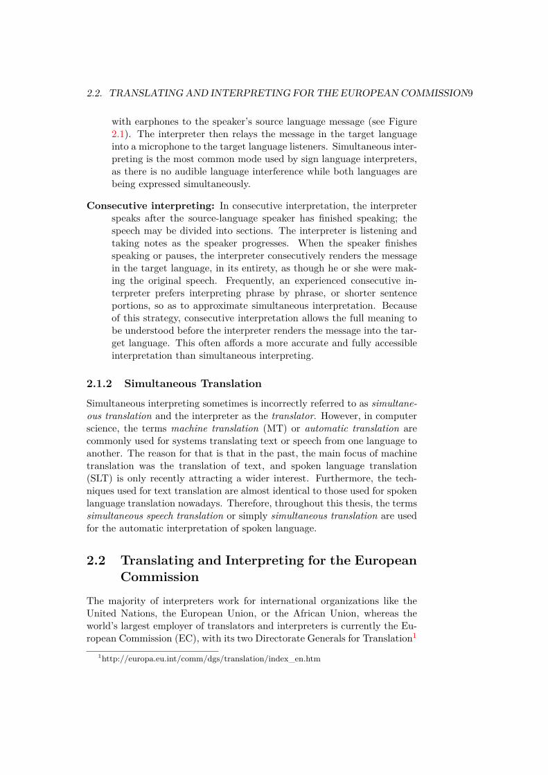
Figure 2.1: Translation booths in the European Parliament’s hemicycle atBrussels (from [Wik07a, Eur]).
speaking the same language. [Wik07b]Both interpreting and interpretation can be used to refer to this activity,
but the word interpreting is commonly used in avoiding the other meaningsof the word interpretation.
The practitioner who orally translates for parties conversing in differentlanguages or in sign language is called an interpreter. Interpreters must con-vey not only all elements of meaning, but also the intentions and feelings ofthe original, source language speaker. In fact, the end result is an interme-diate stage of spoken communication, which aims to allow target languagelisteners to hear, perceive, and experience the message in a way that is asclose as possible to the experience of those who understand the original,source language. [Wik07b]
Translators and interpreters are trained in entirely different manners.Translators receive extensive practice with representative texts in varioussubject areas, learn to compile and manage glossaries of relevant termi-nology, and master the use of both current document-related software (forexample word processors, desktop publishing systems, and graphics or pre-sentation software) and computer-assisted translation software tools. In-terpreters, by contrast, are trained in precise listening skills under taxingconditions, memory and note-taking techniques for consecutive interpreting,and split-attention for simultaneous interpreting. [Wik07c]
The industry expects interpreters to be more than 80% accurate; thatis to say that interpretation is an approximate version of the original. Bycontrast, translations should be over 99% accurate. [Wik07c]
2.1.1 Simultaneous and Consecutive Interpreting
There are two modes of interpretation: simultaneous and consecutive.
Simultaneous interpreting: In simultaneous interpreting, the interpreta-tion occurs while the source language speaker speaks, as quickly as theinterpreter can formulate the spoken message in the target language.At the European Parliament, for example, simultaneous interpretationoccurs while the interpreter sits in a sound-proof booth, while listening
2.2. TRANSLATING AND INTERPRETING FOR THE EUROPEAN COMMISSION9
with earphones to the speaker’s source language message (see Figure2.1). The interpreter then relays the message in the target languageinto a microphone to the target language listeners. Simultaneous inter-preting is the most common mode used by sign language interpreters,as there is no audible language interference while both languages arebeing expressed simultaneously.
Consecutive interpreting: In consecutive interpretation, the interpreterspeaks after the source-language speaker has finished speaking; thespeech may be divided into sections. The interpreter is listening andtaking notes as the speaker progresses. When the speaker finishesspeaking or pauses, the interpreter consecutively renders the messagein the target language, in its entirety, as though he or she were mak-ing the original speech. Frequently, an experienced consecutive in-terpreter prefers interpreting phrase by phrase, or shorter sentenceportions, so as to approximate simultaneous interpretation. Becauseof this strategy, consecutive interpretation allows the full meaning tobe understood before the interpreter renders the message into the tar-get language. This often affords a more accurate and fully accessibleinterpretation than simultaneous interpreting.
2.1.2 Simultaneous Translation
Simultaneous interpreting sometimes is incorrectly referred to as simultane-ous translation and the interpreter as the translator. However, in computerscience, the terms machine translation (MT) or automatic translation arecommonly used for systems translating text or speech from one language toanother. The reason for that is that in the past, the main focus of machinetranslation was the translation of text, and spoken language translation(SLT) is only recently attracting a wider interest. Furthermore, the tech-niques used for text translation are almost identical to those used for spokenlanguage translation nowadays. Therefore, throughout this thesis, the termssimultaneous speech translation or simply simultaneous translation are usedfor the automatic interpretation of spoken language.
2.2 Translating and Interpreting for the EuropeanCommission
The majority of interpreters work for international organizations like theUnited Nations, the European Union, or the African Union, whereas theworld’s largest employer of translators and interpreters is currently the Eu-ropean Commission (EC), with its two Directorate Generals for Translation1
1http://europa.eu.int/comm/dgs/translation/index_en.htm

10 CHAPTER 2. HUMAN SIMULTANEOUS INTERPRETATION
and Interpretation2.The Directorate General for Translation (DGT) mainly provides trans-
lations of written text in and out of the 23 official languages of the EuropeanUnion. There are more than 1800 translators working full-time on translat-ing documents and on other language-related tasks, accompanied by some600 support staff. In 2006, the DGT translated more than 1.5 million pages;72% of the original texts were drafted in English, 14% in French, 2.7% inGerman, and 10.8% in the other 20 EU languages. English and French pre-dominate, because they are the principal drafting languages in the EuropeanCommission. [Dir07b]
To support the translators, information technology, such as translationmemory and machine translation technology, is often used. With transla-tion memory technology, translators can avoid re-translating what has al-ready been translated. At present, the central translation memory containsmore than 84 million phrases in all official EU languages. Machine trans-lation technology (currently available for around 18 language pairs) is usedwhen rapid access to a large amount of information in different languages isneeded, or when some officials would like to draft a document in a languageother than their mother tongue. Machine translation systems are used alsoas a basis for an eventual translation of a document. The amount of cor-recting required varies according to the document type. Speech recognitiontechnology is used as well (currently for only 9 EU languages) for dictatingtext directly in a natural, continuous way, achieving a high degree of accu-racy and efficiency. The ergonomic an health benefits are also obvious, asadverse physical effects associated with intensive typing and mouse use arereduced. [Dir07c]
The Directorate General for Interpretation (DG Interpretation) is theEuropean Commission’s interpreting service and conference organizer, andprovides interpreters for about 50 - 60 meetings per day in Brussels andelsewhere. The language arrangements for these meetings vary considerably— from consecutive interpreting between two languages, for which one in-terpreter is required, to simultaneous interpreting into and out of 23 or morelanguages, which requires at least 69 interpreters. At present, the Councilof the Union accounts for around 46% of the interpreting services provided,followed by the Commission with around 40%. There are more than 500staff interpreters, accompanied by 2700 accredited freelance interpreters.[Dir07a]
When working for the European Commission, translators or interpretersmust have a university-level education, a perfect knowledge of the targetlanguage (usually their mother tongue), and a thorough knowledge of atleast two other official languages.
2http://scic.cec.eu.int/europa/

2.3. CHALLENGES IN HUMAN INTERPRETATION 11
In 20063, the European Parliament has spent approximately 300 millionEuro, i.e. 30% of its budget, for the interpretation and translation of parlia-ment speeches and EU documents. In total, an amount of approximately 1.1billion Euros are spent per year for the translating and interpreting serviceswithin the European Union, which is around 1% of the total EU budget.[VS06]
2.3 Challenges in Human Interpretation
According to [AKESH00], researchers in the field of psychology, linguis-tics and interpretation, like Henderson [Hen82], Hendricks [Hen71] andSeleskovitch [Sel78], seem to agree that simultaneous interpretation is ahighly demanding cognitive task involving a difficult psycholinguistic pro-cess. These processes require the interpreter to monitor, store and retrievethe input of the source language continuously in order to produce the oralrendition of this input into the target language. It is clear that this type ofdifficult linguistic and cognitive operation will force even professional inter-preters to resort to a kind of groping for words, a kind of lexical or syntheticsearch strategy.
2.3.1 Fatigue and Stress
Fatigue and stress affecting the interpreter negatively, leading to a decreasein simultaneous interpretation quality. In a study of the fatigue factor andbehavior under stress during extended interpretation turns by Moser-Mercerand her colleagues [MMKK98], professional interpreters were told to workuntil they could no longer provide acceptable quality. It was shown that:(1) during the first 20 minutes, the frequency of errors rose steadily; (2)the interpreters, however, appeared to be unaware of this decline in quality;(3) at 60 minutes, all subjects combined committed a total of 32.5 meaningerrors; and (4) in the category of nonsense, the number of errors almostdoubled after 30 minutes on the task. Following Moser-Mercer, it can beconcluded “that shorter turns do indeed preserve a high level of quality, butthat interpreters cannot necessarily be trusted to make the right decisionwith regard to optimum time on performing this task (interpreting)”.
Besides extended interpretation turns, other factors influence the inter-pretation quality. In a study by McIlvaine Parsons [Par78], factors rated byinterpreters as stressful are: speakers talking very fast, the lack of clarityor coherence by the speaker, the need for intense concentration e.g. in TV-shows, the inexperience with the subject matter, a speaker’s accent, longspeaker utterances between pauses, background noise, and poor positioningof the speaker’s microphone relative to the speaker. The stress factor was
3Until that time, only 20 official languages were available.

12 CHAPTER 2. HUMAN SIMULTANEOUS INTERPRETATION
also compared between experts and novices in [Kur03]. She came to the con-clusion that “conference interpreters have learned to overcome their stagefright with experience and have developed more tolerance for the stress in-volved in simultaneous interpretation, while student interpreters still grapplewith numerous problems”.
In [Vid97], the conclusion was drawn that interpreters should work inteams of two or more and be exchanged every 30 minutes. Otherwise, the ac-curacy and completeness of simultaneous interpreters decrease precipitously,falling off by about 10% every 5 minutes after holding a satisfactory plateaufor half an hour.
2.3.2 Compensatory Strategies
In experiments with students and professional interpreters Al-Khanji[AKESH00] found that the most frequent compensatory strategies are —in the order of occurrences — skipping, approximation, filtering, compre-hension omission, and substitution. In order to get a deeper insight to thechallenges of simultaneous interpretation for humans the strategies foundduring the experiments in [AKESH00] are summarized shortly.
Skipping: This strategy was used when: (1) the input is incomprehensi-ble for the interpreter; (2) the interpreter decided that the input isrepetitive; or (3) the interpreter was lagging behind the speaker.
Approximation: When there was no time for details, the interpreters at-tempted to reconstruct the optimal meaning by giving a less precisemeaning of a word or an expression in the target language instead ofthe required lexical expression in the source language. Since enoughsemantic components were given in most cases, the meaning of theintended message was not negatively influenced.
Filtering: This strategy was used when the interpreter tried to compressthe length of an utterance in order to find an economic expression. Inso doing, interpreters seemed to preserve the semantic content of themessage. Filtering is different from skipping in that interpreters arenot necessarily facing a problem with the difficulty of economizing byreducing the length of an utterance.
Incomplete Sentences: Unlike skipping, the provision of incomplete sen-tences was used when interpreters omit larger units of speech, whichmay have resulted from a failure in text comprehension. In such cases,the interpreter initially made an attempt to start interpreting units ofspeech, which caused comprehension problems, but then gave up andcut short by stopping in mid-sentence.

2.3. CHALLENGES IN HUMAN INTERPRETATION 13
Substitutions: This strategy was employed when interpreters used a lexi-cal item in the target language which did not communicate the desiredconcept nor did it basically retain the meaning of the item in the sourcelanguage.
2.3.3 Fluency and the Ear-Voice-Span
Since a audience is only able to evaluate the simultaneously interpreted dis-course by its form, the fluency of an interpretation is of utmost importance.According to a study by Kopczynski [Kop94], fluency and style was thirdon a list of priorities of elements rated by speakers and attendees that con-tribute to quality, after content and terminology. Following the overview in[Yag00], an interpretation should be as natural and as authentic as possible,which means that artificial pauses in the middle of a sentence, hesitations,and false-starts should be avoided [Jon98] and the tempo and intensity ofthe speaker’s voice should be imitated [Kop94].
Another point to mention is the time span between a source languagechunk and its target language chunk, which is often referred to as ear-voice-span, delay, or lag. Following the summary in [Yag00], the ear-voice-spanis variable in duration depending on some source and target language at-tributes, such as speech delivery rate, information density, redundancy, wordorder, syntactic characteristics, etc. Nevertheless, the average ear-voice-spanfor certain language combinations has been measured by many researchers,and varies largely from two to six seconds [Bar69, Led78], depending on thespeaking rate. Short delays are usually preferred for several reasons. Theaudience is for example irritated when the delay is too large and is soonasking whether there is a problem with the interpretation. Another reasonis that a short delay facilitates the indirect communication between the au-dience and the speaker but also between people listening to the interpreterand to the speaker. Therefore, interpreters tend to increase their speakingrate when the speaker has finished.
2.3.4 Techniques for Simultaneous Interpretation
Seleskovitch [Sel78], a professional interpreter and instructor for interpreters,advocates retaining the meaning of the source language utterance, ratherthan the lexical items, and argues that concepts (semantic storage) are fareasier to remember than words (lexical storage). Semantic storage also al-lows the interpreter to tap into concepts already stored in the brain, whichallows the interpreter to hitch a “free ride” on the brain’s natural language-generation ability, by which humans convert concepts to words seeminglyautomatically. For this reason, preparation before a conference, by talkingto the speaker and by researching the domain of the talk, is vital for inter-preters. But Seleskovitch admits that concept-based interpretation may not

14 CHAPTER 2. HUMAN SIMULTANEOUS INTERPRETATION
always be possible. If the interpreter is unable to understand the conceptbeing translated, or is under particular stress, they may resort to word-for-word translation. According to Moser-Mercer [MM96], also a professionalinterpreter and teacher and active in interpretation research, simultaneousinterpretation must be as automatic as possible — there is little time foractive thinking processes. The question is not avoiding mistakes — it israther correcting them and moving on when they are made. Another sug-gestion for interpreters from Hönig [Hö97] is that interpreters, who mustkeep speaking in the face of incomplete sentences, must either “tread water”(stall while waiting for more input) or “take a dive” (predict the directionof the sentence and begin translating it). He suggests that “diving” is notas risky as it sounds, provided the interpreter has talked with the speakerbeforehand, and has what he calls a “text map” of where the talk is headed.[Loe98]
Chapter 3
Automatic SimultaneousTranslation
A speech translation system consists of two major components: speech recog-nition and machine translation. Words in the recorded speech input are rec-ognized and the resulting hypothesis is transmitted to the machine transla-tion component, which outputs the translation. While this sounds relativelyeasy, especially for simultaneous translation which require real-time and lowlatency processing with good translation quality, several problems have tobe solved. Furthermore, automatic speech recognition and machine trans-lation, which have evolved independently from each other for many years,have to be brought together.
Recognizing speech in a stream of audio data is usually done utteranceper utterance, where the utterance boundaries have to be determined withthe help of an audio segmenter before they can be recognized. Especiallywhen the audio data contains noise artifacts or even cross-talk1, this strat-egy can be extremely useful, because such phenomena can be removed inadvance, leading to an improvement in ASR performance. However, thetechniques used in such audio segmenters often require global optimizationover the whole audio data and are therefore infeasible for a simultaneoustranslation system. On the other hand, even a simple speech/ non-speechbased audio segmenter will introduce additional latency, since the classifica-tion of speech/ non-speech frames has to be followed by a smoothing processto remove mis-classifications.
Almost all machine translation systems currently available were devel-oped in the context of text translation and have to cope with differencesbetween a source and target language such as different amount and usageof word ordering, morphology, composita, idioms, and writing style, butalso vocabulary coverage. Only recently has spoken language translation
1With cross-talk, speech from others in the background, which is recorded by thespeaker’s microphone is defined.
15

16 CHAPTER 3. AUTOMATIC SIMULTANEOUS TRANSLATION
attracted wider interest. So, in addition to the differences between a sourceand target language, spoken language differs from written text in style.While text can be expected to be mostly grammatically correct, spoken lan-guage and especially spontaneous or sloppy speech contains many ungram-maticalities, including hesitations, interruptions, and repetitions. In addi-tion, the choice of words and the amount of vocabulary used differ betweentext and speech. Another difference is that utterances are demarcated inwritten text, using punctuation, but such demarcation is not directly avail-able in speech. This is a problem, because traditionally almost all machinetranslation systems are trained on aligned bilingual sentences, preferablywith punctuation, and therefore are expecting sentences as input utterancesin the same style. But when a low latency speech translation system isrequired, sentences are not an appropriate unit, because especially in spon-taneous speech they tend to be very long — up to 20-30 words. To cope withthis problem, a third component is introduced, which tries to reduce the la-tency by resegmenting the ASR hypotheses into smaller chunks without adegregation in translation quality. Chapter 8 describes this component inmore detail.
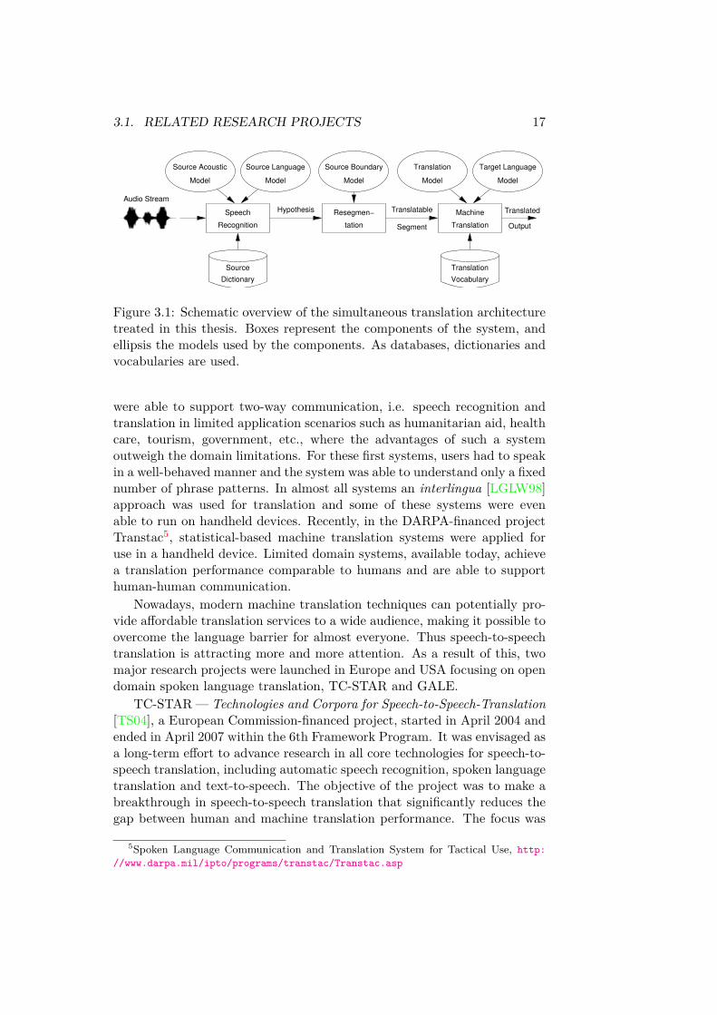
Figure 3.1 gives a schematic overview of the simultaneous translation ar-chitecture treated in this thesis together with required databases and mod-els. From the continuous input stream of speech, the ASR component isproducing a continuous stream of partial first-best hypotheses, which areresegmented into appropriate chunks for the SMT component. The SMTcomponent translates each of these source language chunks into the targetlanguage. By using multiple SMT components translation can be done inparallel into different target languages at the same time. For deliveringthe translation output, different technologies may be used among which themost prominent are either subtitles or speech synthesis. A more detaileddescription will be given in Chapter 9.
In the next section, some related research projects will be described.Compared to the previous chapter, the advantages of automatic simultane-ous translation over human interpretation will be discussed in Section 3.2.The demands on such a system will be formulated in Section 3.3. Finally,in Section 3.4, an overview of some application scenarios in which such asystem could be of use are described.
3.1 Related Research Projects
In the past, systems developed within research projects and consortia such asC-Star2, Verbmobil3, Nespole4, Enthusiast, Digital Olympics, and Babylon
2Consortium for Speech Translation Advanced Research, http://www.c-star.org3http://verbmobil.dfki.de4Negotiating through Spoken Language in E-Commerce, http://nespole.itc.it
3.1. RELATED RESEARCH PROJECTS 17
Dictionary
Source
Hypothesis Translatable
Segment
Model
Source Boundary
Resegmen−
tationRecognition
Speech
Translation
Model Model
Target Language
Machine
Translation
Model
Source Acoustic
Model
Source Language
Output
Translated
Translation
Vocabulary
Audio Stream
Figure 3.1: Schematic overview of the simultaneous translation architecturetreated in this thesis. Boxes represent the components of the system, andellipsis the models used by the components. As databases, dictionaries andvocabularies are used.
were able to support two-way communication, i.e. speech recognition andtranslation in limited application scenarios such as humanitarian aid, healthcare, tourism, government, etc., where the advantages of such a systemoutweigh the domain limitations. For these first systems, users had to speakin a well-behaved manner and the system was able to understand only a fixednumber of phrase patterns. In almost all systems an interlingua [LGLW98]approach was used for translation and some of these systems were evenable to run on handheld devices. Recently, in the DARPA-financed projectTranstac5, statistical-based machine translation systems were applied foruse in a handheld device. Limited domain systems, available today, achievea translation performance comparable to humans and are able to supporthuman-human communication.
Nowadays, modern machine translation techniques can potentially pro-vide affordable translation services to a wide audience, making it possible toovercome the language barrier for almost everyone. Thus speech-to-speechtranslation is attracting more and more attention. As a result of this, twomajor research projects were launched in Europe and USA focusing on opendomain spoken language translation, TC-STAR and GALE.
TC-STAR— Technologies and Corpora for Speech-to-Speech-Translation[TS04], a European Commission-financed project, started in April 2004 andended in April 2007 within the 6th Framework Program. It was envisaged asa long-term effort to advance research in all core technologies for speech-to-speech translation, including automatic speech recognition, spoken languagetranslation and text-to-speech. The objective of the project was to make abreakthrough in speech-to-speech translation that significantly reduces thegap between human and machine translation performance. The focus was
5Spoken Language Communication and Translation System for Tactical Use, http://www.darpa.mil/ipto/programs/transtac/Transtac.asp

18 CHAPTER 3. AUTOMATIC SIMULTANEOUS TRANSLATION
on the development of new algorithms and methods. The project targeteda selection of unconstrained conversational speech domains – speeches andbroadcast news – and three languages: European English, European Span-ish, and Mandarin Chinese. Project partners, mainly involved in speechrecognition and/ or machine translation, were the Bruno Kessler Founda-tion (formerly ITC-IRST), the RWTH Aachen, LIMSI-CNRS, the Universi-tad Politècnica de Catalunya (UPC), Universität Karlsruhe (TH), and IBM.
The goal of the DARPA GALE – Global Autonomous Language Exploita-tion [GAL05] program is to develop and apply computer software technolo-gies to absorb, analyze and interpret huge volumes of speech and text inmultiple languages. Automatic processing engines will convert and distill thedata, delivering pertinent, consolidated information in easy-to-understandforms to military personnel and monolingual English-speaking analysts inresponse to direct or implicit requests. In difference to TC-STAR, the out-put of each engine is English-translated text only and no speech synthesis isused. Instead, a distillation engine is responsible for integrating informationof interest to its user from multiple sources and documents. The input to thetranscription engine is speech, currently with a main focus on Arabic andChinese. Military personnel will interact with the distillation engine viainterfaces that could include various forms of human-machine dialog (notnecessarily in natural language).
GALE evolved from two other past projects, EARS and TIDES. Thegoal of the EARS – Effective, Affordable, Reusable Speech-to-Text programwas to “produce powerful new speech-to-text (automatic transcription) tech-nology whose outputs are substantially richer and much more accurate thancurrently possible. The program focused on natural, unconstrained human-human speech from broadcasts and telephone conversations in a number oflanguages. The intent was to create core enabling technology suitable for awide range of advanced applications, but not to develop those applications.Inputs and outputs will be in the same language.” The TIDES – Translin-gual Information Detection, Extraction and Summarization program insteaddeveloped robust technology for translingual information processing. Thegoal was “to revolutionize the way that information is obtained from hu-man language by enabling people to find and interpret needed information,quickly and effectively, regardless of language or medium.” TIDES tasksincluded information detection, extraction, summarization and translationfocusing mainly on English, Chinese and Arabic.
Another project to mention is CHIL – Computers in the Human In-teraction Loop. CHIL aimed in making significant advances in the fieldsof speaker localization and tracking, speech activity detection and distant-talking automatic speech recognition. Therefore, in addition to near andfar-field microphones, seminars were also recorded by calibrated video cam-eras. The long-term goal was the ability to recognize speech in a real rever-berant environment, without any constraint on the number or distribution

3.2. ADVANTAGES OF AUTOMATIC SIMULTANEOUS TRANSLATION19
Figure 3.2: Comparison of automatic translation and human interpretationperformance judged by humans in the project TC-STAR. [HMC07]
of microphones in the room nor on the number of sound sources active atthe same time.
Parts of this thesis evolved within the two projects CHIL and TC-STAR.
3.2 Advantages of Automatic Simultaneous Trans-lation
Given the explanations in the previous chapter of human interpretation ingeneral and in the European Commission in particular, one has to weigh twofactors when considering the use of simultaneous translation systems: costand translation quality. The comparative results of TC-STAR in Figure 3.2[HMC07] between human interpretation and automatic speech translationshow that automatic translation was judged worse than human interpreta-tion in most categories, but when it comes to the transfer of content bothwere judged nearly equally good. The reason why human interpretationdoes not reach “perfect” results is because often interpreters make use ofthe above mentioned compensatory strategies. On the other hand, even theautomatic translation system can be of great help, especially for people notunderstanding the speaker’s language at all. Furthermore, an automaticsystem can easily make use of additional information available about thespeaker or the topic of the speech by using adaptation techniques to im-prove its perfomance. Note that the automatic TC-STAR system used forthe comparison above was not working in real-time. This means that for asimultaneous translation system which has to deliver the translations witha latency as small as possible, a degregation in translation quality can beexpected.
Another advantage of a simultaneous translation system compared toa human interpreter is that memorizing is not a problem for the system.Therefore the compensatory strategies skipping, approximation, or incom-

20 CHAPTER 3. AUTOMATIC SIMULTANEOUS TRANSLATION
plete sentences described in Section 2.3 will not be needed, independentlyof the speaking rate of the speaker. However, depending on the system’stranslation speed it might be possible that the latency will rise. While itmight be possible for humans to compress the length of an utterance with-out destroying the meaning, i.e. filtering or summarization, it is still a verychallenging task for automatic systems [Fur07, Man01].
Another argument is that simultaneous interpretation at 300 to 400 Eu-ros per hour, is quite expensive. The reason for that is that usually two inter-preters are necessary and that the time for preparation and postprocessingmust be considered additionally. Furthermore, simultaneous interpretationrequires a soundproof booth with audio equipment, which can be rented, butthis incurs additional costs which may be in most cases unsuitable for smallevents. On the other hand, a simultaneous translation system needs timeand effort for preparation and adaptation towards the target application,language and domain. Depending on the required translation quality, thecosts therefore can exceed those for a human interpretation. However, themajor advantage of an automatic system is that once it is adapted, it can beeasily re-used in the same domain, language etc. A single laptop togetherwith a microphone is sufficient.
To some extent even generalization should not be a problem for auto-matic systems. Due to the way such systems are trained, expressions notdirectly within the required domain but closely related to it are alreadycovered by the system. Furthermore, adaptation techniques can be used toextend the coverage and quality.
Especially in situations where a simultaneous translation into multiplelanguages is required, an automatic system is advantageous, because onlythe translation has to be extended to a new target language, while the sourceside recognition and resegmentation component of the system can be keptunchanged.
Another advantage is that the transcript of a speech or lecture is pro-duced for free by using an automatic system in the source and target lan-guages. In the European Union, for example, these transcripts can be usedas an initial version of the protocols which have to be prepared anyway.
3.3 Demands on Automatic Simultaneous Trans-lation
In comparison to other translation systems, and also given the observationsregarding human interpretation in the previous chapter, four main demandson an automatic simultaneous translation system can be formulated:
• correct content
• correct syntax
3.4. APPLICATION SCENARIOS – THE LECTURE SCENARIO 21
• high fluency
• low latency
Obviously, a correct content is the most important demand on a simultane-ous translation system. In connection to this, syntax also plays an importantrole, because the wrong syntax can destroy the content of a sentence. Nev-ertheless, to understand the content, a translation need not be completelycorrect. Instead, it may be sufficient if the words carrying the content ormeaning of a sentence are correctly translated and no misleading content doexist.
Fluency on the other hand, requires that a simultaneous translation sys-tem produce a translation which is as natural as possible. Both content andsyntax contribute to naturalness to some extent, but hesitations, false-starts,and other disfluencies, all characteristics of spontaneous speech, should alsobe removed either in advance or during translation [RLS07a]. Imitating thespeaker’s tempo also contributes to higher fluency, but also influences thelatency. As already clarified in Section 2.3, it is important to keep the la-tency, i.e. the ear-voice-span of the whole system, as short as possible. InEnglish, a latency of about two to six seconds is equivalent to a delay ofabout 4 to 12 words, since the average speaking rate is about 120 words perminute [RHP03, YLC06].
A comparable simultaneous translation system should therefore be ableto produce speech translations of sufficient quality in real-time with a lowlatency.
3.4 Application Scenarios – The Lecture Scenario
Given the limitations of the recognition and translation capabilities of cur-rent speech translation systems, and the system development costs comparedto human interpreters, possible application scenarios for simultaneous trans-lation are restricted to domains to which a system can be well adapted andapplications in which a system can be re-used and modified or customizedwith less effort. Therefore, the lecture scenario is selected as target sce-nario for this thesis, in which a single speaker is talking about a specifictopic to a larger audience (see Figure 3.3). Small talks, student seminars orparliamentary speeches also belong to this scenario.
Other environments in which such a system could be of great use aretelephone conversations and meetings. In both situations, it would allowpeople to communicate with each other independently of the language bar-riers. Telephone conversations and meetings are highly spontaneous dialogsand discussions between two or more people focusing on different topics andtherefore difficult for both speech recognition and machine translation. Fur-thermore, a very low-latency simultaneous translation system is required

22 CHAPTER 3. AUTOMATIC SIMULTANEOUS TRANSLATION
Figure 3.3: The lecture scenario. The speaker in front of the audience isrecorded with the help of a microphone. The speech is transferred to thesimultaneous translation system running on a PC or laptop and translated.The figure shows also different possibilities of how the translation outputcan be delivered to the audience: as subtitles on the projection screen, byusing loudspeakers, or projected into heads-up display goggles.

3.4. APPLICATION SCENARIOS – THE LECTURE SCENARIO 23
because otherwise direct communication between the participants will behindered. Thus, automatic simultaneous translation in these environmentswill remain challenging for several years.

24 CHAPTER 3. AUTOMATIC SIMULTANEOUS TRANSLATION

Chapter 4
A First Baseline System
This chapter introduces a first baseline system for spoken language trans-lation of lectures and speeches. This system will be suitable for consecu-tive translation only; the necessary techniques for supporting simultaneoustranslation will be presented later in Chapters 5 – 8. Starting from speechrecognition and machine translation systems developed and used successfullyin the context of the NIST RT-06S Rich Transcription Meeting Evaluationon lecture meetings and of the 2007 TC-STAR Evaluation on European Par-liamentary Speeches, it will be shown how a first baseline spoken languagetranslation system was built. It will be analyzed how both, the lecturesrecorded within CHIL and the speeches recorded within TC-STAR compareto the lectures on which we focus in this thesis with respect to recognitionand translation quality.
The NIST Rich Transcription Meeting Evaluation series focused on therich transcription of human-to-human speech, i.e. speech-to-text and metadata extraction with the goal to develop recognition technologies that pro-duce language-content representations (transcripts) which are understand-able by humans and useful for downstream analysis processes. The eval-uation in 2006 (RT-06S1) was supported by two European projects, AMI– Augmented Multi-party Interaction2 and CHIL – Computers in the Hu-man Interaction Loop [WSS04]. Therefore, two data tracks were availableon which a system could be evaluated: Conference Meetings and LectureMeetings. In both data tracks, the speakers were recorded with close andfar-field microphones, i.e. table-top microphones and microphone arrays.Conference meetings (supported by AMI) are goal-oriented small confer-ence meetings like group meetings and decision-making exercises involving4-9 participants, who are usually sitting around a table. In contrast, lec-ture meetings (supported by CHIL) are educational events, where a singlelecturer is briefing an audience on a particular topic.
1http://www.nist.gov/speech/tests/rt/2006-spring/2http://www.amiproject.org/
25

26 CHAPTER 4. A FIRST BASELINE SYSTEM
The European Parliament Plenary Speech (EPPS) task within TC-STARfocuses on transcribing speeches in the European Parliament in English andSpanish, and translating and synthesizing them into the other language.For the speech-to-text task, the data has been recorded from the Euro-pean Union’s TV Information service Europe by Satellite (EbS) 3, whichbroadcasts the sessions of the European Parliament live using separate au-dio channels for the speaker as well as for the simultaneous interpretationsinto all official EU languages [GBK+05]. Thus, the audio recordings containspeech from the politicians at their seats and at the podium using standmicrophones, and speech from the interpreters using head-sets. For spokenlanguage translation, the final text editions from the European Parliamentare available through the EuroParl web site 4.
Since lectures and speeches are usually given in rooms with a large au-dience, microphones with a small distance to the speaker’s mouth, such ashead-worn or directional stand microphones are preferred over far-field mi-crophones which are more sensitive to background noise. Therefore, thespeech recognition systems were developed and optimized with respect toclose-talk recording conditions. Since this thesis evolved in the context ofthe European projects CHIL and TC-STAR, European accented English wasof particular interest.
In Section 4.1 lectures and speeches are characterized by their spontane-ity and difficulty for speech recognition and spoken language translation andcompared to other speech data such as recordings of read speech, broadcastnews and meetings. After describing the training, test and evaluation dataused for the speech recognition and machine translation systems and exper-iments in Section 4.2, the development of a first baseline speech-to-speechtranslation system is shown. For this purpose, a first speech recognitionsystem is presented in Section 4.3 and, second, a first statistical spoken lan-guage translation system is introduced in Section 4.4. The performance, i.e.the recognition and translation quality and speed is measured and compared.
4.1 Characterization of Lectures and Speeches
In comparison to speeches given in parliament plenary sessions such as thosein the European Parliament, lectures or talks are generally more difficult forspeech recognition. The reason for that is that although potentially prac-ticed in advance, lectures or talks are usually given freely and are thereforemore spontaneous, thus containing more disfluencies and ungrammatical-ities. In contrast, the speeches given in parliament plenary sessions arewell prepared and often read. Furthermore, while the speeches given inparliament plenary sessions must be understandable for all politicians, the
3Europe by Satellite, http://europa.eu.int/comm/ebs/index_en.html4The European Parliament Online, http://www.europarl.europa.eu

4.1. CHARACTERIZATION OF LECTURES AND SPEECHES 27
Figure 4.1: NIST benchmark comparison (from [FA07]). The speech recog-nition quality on tasks was measured in word error rate (WER).
level of detail in lectures or talks can be targeted to the audience, rangingfrom general understandable to very specific. E.g. the lectures recorded inCHIL are very technical oriented. On the other hand, when compared tomeetings, both lectures and speeches are less spontaneous, more focused,and are mainly monologues with only small amounts of discussion, i.e. thequestion-and-answer part.
Figure 4.1 shows the evolution of word error rates over the years in speechrecognition for several NIST-organized benchmarks. The results on Euro-pean English lectures and parliament speeches were added from the projectsCHIL and TC-STAR. From the figure, it can be observed that speech recog-nition quality decreases with an increasing amount of spontaneity in thespeaking style and with domain complexity. The higher word error rates(see Section 4.2.5) for lecture meetings compared to meetings can be ex-plained by the higher amount of research effort spent on meetings.
In an internal technical report [WB01], Burger analyzed the speakingstyle characteristics in the Translanguage English Database (TED), talksrecorded at the Eurospeech Conference in 1993. Out of the corpus 51speeches, between 5 to 22 minutes long, spoken by 48 individual speak-ers (37 male, 11 female) who originate from 14 different countries was used.

28 CHAPTER 4. A FIRST BASELINE SYSTEM
The speeches were categorized according to the English skill of the speakerand whether the speech was spontaneous or read. She observed that speak-ing rates decrease with English skill and are lower for read speech than forspontaneous presentations. Furthermore, the percentage of filled pauses, i.e.hesitations, and the percentage of corrections, i.e. fragments, repetitions,and false starts, were analyzed. The results showed that read speeches con-tained a lower frequency of filled pauses and corrections when compared tospontaneous ones, and that the amount of filled pauses and corrections in-creases with decreasing English skill. For average non-native English speak-ers, there were approximately 8% filled pauses and 6% corrections in thewords spoken, while for native speakers the respective amounts were about4% in both cases.
Unfortunately, there is no benchmark comparison available for (statis-tical) machine translation, since extensive benchmarking between differentresearch sites for MT is relatively new, and differences in MT results aremore due to the target language than the domain. However, a huge system-atical analysis was done by Koehn for European languages on a corpus ofEuropean Parliament Plenary Sessions [Koe05]. He compared the transla-tion scores for SMT systems for all language pairs of 11 different languages.Figure 4.2 shows some of the results for translation from and into English.It can be seen that for the language pair English-Spanish, which is usedfor the simultaneous translation system in this thesis as well, almost thebest translation scores could be achieved. One reason for that is certainlythat this language pair has been most heavily investigated by the researchcommunity.
4.2 Training, Test and Evaluation DataIn this section, the data used for training the acoustic, translation and lan-guage models of the speech recognition and machine translation systems isdescribed. Furthermore, the details of the development data as well as theevaluation data used to tune the systems and for performing the experimentsdescribed in the following chapters are given.
4.2.1 Acoustic Model Training Data
As already mentioned in the introduction to this chapter, spontaneous, close-talk, European accented English is the focus of this thesis. Based on someexperiments ([FIK+06, FKB+06]) for acoustic model training, recordingsfrom meetings, European Parliament Speeches, lectures and student semi-nars were selected.
ICSI 72h of meetings recorded by the International Computer Science Insti-tute (ICSI) with head-mounted and far-field microphones. The corpus

4.2. TRAINING, TEST AND EVALUATION DATA 29
0
5
10
15
20
25
30
35
DanishGerman
GreekSpanish
FrenchFinnish
ItalianDutch
Portuguese
Swedish
BLEU
from Englishto English
Figure 4.2: Machine translation results on European Parliament PlenarySessions for translation between English and other European languages(from [Koe05]). Machine translation quality was measured automaticallyand are given in BLEU scores (see Section 4.2.5).

30 CHAPTER 4. A FIRST BASELINE SYSTEM
Type Meetings Speeches LecturesICSI NIST EPPS uEPPS TED Seminars
Duration [hrs] 72 15 80 167 10 10Speakers 53 61 1894 2982 52 67Recordings 75 19 63 74 39 17
Table 4.1: Summary of the data used for acoustic model training.
contains a significant portion of non-native English speakers, varyingin fluency from nearly-native to challenging-to-transcribe [JAB+04]
NIST 13h of meetings recorded by the National Institute of Standardsand Technology (NIST) with head-mounted and far-field micro-phones. This corpus contains mostly native American English speakers[GLM+04].
EPPS-S 80h of European parliament plenary sessions (EPPS) recordedwithin the TC-STAR project containing mostly non-native EuropeanEnglish speakers [GBK+05].
EPPS-U 80h of European parliament plenary sessions (EPPS) recordedand transcribed automatically by RWTH Aachen within TC-STAR[GHSN07].
TED 10h of lectures recorded at Eurospeech 1993. The TranslanguageEnglish Database (TED) audio recordings have non-native Englishspeakers presenting academic papers for approximately 15 minuteseach [LSF+94, Cond].
SMNR 10h of mostly student seminars recorded within the CHIL projectwith head-mounted and far-field microphones, most of which were pre-sented by non-native European English speakers [WSS04].
The most suitable data for lecture recognition are the lectures and sem-inars collected in the CHIL project (SMNR) and the Translanguage EnglishDatabase (TED). Since the amount of data is insufficient to train acousticmodels which perform well in large vocabulary speech recognition tasks suchas lecture recognition, other data has to be used as well. The meeting dataconsists of recordings of highly spontaneous meeting speech from mostlynative English speakers collected at three different sites: ICSI, NIST andCMU. In contrast, the European Parliament data covers non-native, usuallywell prepared speeches. An overview of the details of the several trainingcorpora is given in Table 4.1.

4.2. TRAINING, TEST AND EVALUATION DATA 31
English SpanishSentences 1,162,176Words 27.7M 28.9MVocabulary 93,157 130,473Singletons 34,543 45,400
Table 4.2: Summary of the bilingual data used for training the machinetranslation system.
4.2.2 Translation Model Training Data
The baseline translation system was trained on a corpus of sentence-aligned,parallel final text editions from the European Parliament, available throughits web site. The data was crawled, pre-processed and sentence-alignedautomatically by RWTH Aachen [GBK+05]. The corpus statistics of thepre-processed EPPS training corpora are shown in Table 4.2.
4.2.3 Language Model Training Data
The language models for the baseline speech recognition systems weretrained on the corpora used for the RT-06S and 2007 TC-STAR evalua-tion systems [FIK+06, SFH+06]. Three different types of data were used:speech transcripts, written text, and text data collected from the world wideweb5. Altogether, the following English corpora were available:
EPPS-S 750k words of EPPS transcriptions in non-native English[GBK+05]
EPPS-T 33M words of EPPS final text editions [GBK+05]
EPPS-U 1.4M words of automatically transcribed speech data [GHSN07]
MTG 1.1M words of meeting transcriptions (ISL, ICSI, NIST, LDC) mostlyin non-native English [Con04]
AMI 200k words of meeting transcriptions from the AMI project of mostlynon-native English [CAB+05]
TED 98k words of transcriptions from the Translanguage English Databasecontaining talks held at Eurospeech 1993 in non-native English[LSF+94]
SMNR 45k words of seminar transcriptions from the project CHIL in non-native English [WSS04]
5More details on the web-collection will be given in the Chapters 4 and 6

32 CHAPTER 4. A FIRST BASELINE SYSTEM
SWB 4M word of transcriptions from Switchboard [(LD]
BN 131M words of broadcast news written text data [Cona]
UN 42M words of the English part of the United Nations Parallel TextCorpus v1.0 [Cone]
HNSRD 48M words of text data consisting of U. K. parliament debates[Conc]
GWRD 167M words of text data extracts from the Gigaword corpus [Conb]
PROC 23M words out of recent speech and translation related conferenceproceedings from 2002 until 2005
UW-M 147M words of data collected from the web by the University ofWashington related to ISL, ICSI, and NIST meetings
UKA-M 124M words of data collected from the web by ourselves relatedto MTG and PROC
UKA-L 146M words of data collected from the web by ourselves related toSMNR
UKA-LP 130M words of query-based filtered data collected from the webby ourselves related to SMNR and PROC
UKA-MP 124M words of query-based filtered data collected from the webby ourselves related to MTG and PROC
For the machine translation systems, the same parallel data for languagemodel training was used as described above in Section 4.2.2.
4.2.4 Development and Evaluation Data
For development and evaluation, an amount of 19 lectures and talks ondifferent topics of a single non-native speaker were collected in differentenvironmental conditions. This data is further referred to as lectures. Table4.3 gives an overview of the data.
While lectDev and lectEval were used for system development and eval-uation, lectOther was used for adaptation experiments. IDs referring totalks start with a ’t’ and to lectures with an ’l’. All lectures are given aspart of a course related to the field of speech and language processing atthe university. The talks instead were given for different reasons such askeynotes, press conferences, project reviews, or just an overview about thework done at our research lab. Therefore, the talks are more general and donot have the same level of detail as compared to the lectures. An exception

4.2. TRAINING, TEST AND EVALUATION DATA 33
Talk/ Lecture Duration [min] Words Translationl003 77 12316t012 44 7833
lectDev t032 71 11566t035 32 5519 SPAt041 12 1979 SPAt042 7 1192 SPA∑
243 40405l043 44 7745 SPAt036 32 4824 SPA
lectEval t037 16 2339 SPAt038 51 4673 SPAt044 29 4523∑
172 24104l005 69 11049t010 64 11169t011 11 1931
lectOther t033 49 7507t034 80 12539t039 7 1128 SPAt040 8 1356 SPAt043 7 1072 SPA∑
295 47751
Table 4.3: Partitioning of the available lectures/ talks into development andevaluation data, as well as a comparison of the duration and number of wordper lecture. Lectures for which a translation into Spanish was available aretagged with SPA.

34 CHAPTER 4. A FIRST BASELINE SYSTEM
constitutes the longer talks t032, t033, and t034 which were part of a courseabout speech and language processing for which the lecturer was invited.
As can be seen in Table 4.3, human translations were available for alimited amount of talks and lectures only. In addition, the amount of trans-lations per sentence were restricted to only one. Therefore, the machinetranslation was developed and evaluated on a subset of lectDev, lectEval,and lectOther only. To limit the necessary effort for the human evaluationthis set was reduced even more to t036, t037 and t038 summing up to 92minutes and 14,908 words. Due to the fact that t036 and t037 were givenafter another, the combination of both is often referred to as t036+.
Since there was a recording problem in t010, this talk was not used foracoustic model adaptation.
In addition, some speech recognition experiments were performed on theofficial development and evaluation sets of the TC-STAR-07 EPPS evalua-tion, further referred to as parliamentary speeches, and the lecture meetingdata track of the NIST RT-06S evaluation, further referred to as lecturemeetings. Especially the lecture meetings are well suitable as an additionaldevelopment set because of their similarity in speaking style and focus on aparticular topic. However, the level of detail is even higher than the averagein lectDev and lectEval, and many of the recorded speakers have a strongforeign accent. Compared to the talks and lectures introduced above, bothcharacteristics are responsible for a more difficult recognition.
Moreover, prior to decoding all lecture meeting and EPPS data have tobe automatically segmented. As a result of this, segment boundaries do notnecessarily match with sentence breaks and depending on the segmentationalgorithm and recordings, the segmentation algorithm might fail and clas-sifies speech as non-speech or vice versa. Both might result in additionalrecognition errors. A special care has also to be taken with cross-talk. Ifthis is classified as speech belonging to the current speaker, the recognizedspeech will count as errors. The question-and-answer part also included inthe lecture meeting data makes this even more difficult. As will be seenlater, this explains the much higher word error rates for the lecture meet-ings compared to the talks and lectures. For the details of the differentsegmentation approaches used, we refer to [LFS07, FIK+06, SFH+06]. Thedetails of the different development and evaluation data are presented inTable 4.4.
4.2.5 Performance Measures
The overall performance of a simultaneous translation system always de-pends on the performance of its sub-components, i.e. speech recognition,resegmentation, machine translation, and speech synthesis. Furthermore,since the components are connected in series, errors introduced by one com-ponent are usually amplified by subsequent components.

4.2. TRAINING, TEST AND EVALUATION DATA 35
ID Duration [min] Words Speakers RecordingsDev RT-06Sdev 150 22258 24 67
EPPSdev 192 28976 44 7Eval RT-06Seval 190 21243 70 70
EPPSeval 180 30362 41 5
Table 4.4: Additional development data. RT-06Sdev is identical to theRT-05S evaluation data, EPPSdev is identical to the 2006 TC-STAR de-velopment set, and EPPSeval is identical to the 2007 TC-STAR evaluationset.
The system’s performance can always be judged by humans. However,human evaluations are very time-consuming and costly, and, especially fortechnical oriented lectures, the results often depend on the backgroundknowledge of the evaluators. As a result automatically computable per-formance measures are preferred especially during system development, toaccelerate the turn-around-time of the necessary experiments. Furthermore,they provide a convenient way for comparing different systems.
In the following, some automatically computable performance measureswill be described. They are used in this thesis to judge the quality andspeed of the sub-components of the simultaneous translation system, as wellas the system’s overall latency. It should be noted that, besides the below-mentioned performance measures, also other measures exist in the literature.
PPL The perplexity is a measure of language model performance and isbased on the entropy, a measure of uncertainty associated with a ran-dom variable in the field of information theory [Sha48]. Given a se-quence of words w1, w2, . . . , wm from a vocabulary V, the entropy His defined as
H = − limn→∞
1m
∑w1,...,wm
(P (w1, . . . , wm) log2 P (w1, . . . , wm)) . (4.1)
The summation over all possible word sequences can be discarded un-der the assumption that the source is ergodic and given a large enoughvalue of m, H can be approximated by
H = − 1m
log2 P (w1, w2, . . . , wm). (4.2)
Using this approximation, the perplexity of a language model can bedefined as
PPL = 2H = P (w1, w2, . . . , wm)1m , (4.3)
where P (w1, w2, . . . , wm) is the probability estimate of the word se-quence by the language model.

36 CHAPTER 4. A FIRST BASELINE SYSTEM
OOV-Rate Given a vocabulary V and a text corpus C, the OOV-Rateis defined as the percentage of word occurrences in C which are notcovered by the vocabulary V
OOV = 100 ∗
∑∀w∈C
{1 , w /∈ V0 , otherwise∑∀w∈C
1. (4.4)
WER The word error rate (WER) is the standard metric to measure thequality of a speech recognition system. It is derived from the Leven-shtein or minimum edit distance and is defined as the minimum editdistance between a given hypothesis and its reference transcriptionnormalized by the length N of the reference transcription in words.The minimum edit distance is defined as the minimum number ofsubstitutions S, deletions D, and insertions I of words required totransform the hypothesis into the reference transcription.
WER = S +D + I
N. (4.5)
BLEU The BLEU score [PRWZ02] together with the NIST score [Dod02]are the standard metrics for automatically measuring the quality of amachine translation system. Both are based on the idea of a modifiedn-gram precision based on n-gram co-occurrence statistics. BLEU isdefined as the geometric mean of modified n-gram precision scores pnmultiplied by a brevity penalty. By rearranging the original publishedformula [Dod02], BLEU can be formulated as
BLEU = exp(
N∑n=1
wn log (pn)−max(L∗refLsys
− 1, 0))
, (4.6)
where uniform weights wn = 1/N and n-grams up to length N areusually used. L∗ref is the number of words in the reference translationthat is closest in length to the translation being scored – which becomesimportant when the scoring is done against multiple references – andLsys is the number of words in the translation being scored. Themodified n-gram precision pn is defined as
pn =
∑i
the number of n-grams in segment i, in thetranslation being evaluated, with a matching
reference co-occurrence in segment i
∑i
(the number of n-grams in segment iin the translation being evaluated
) . (4.7)

4.2. TRAINING, TEST AND EVALUATION DATA 37
NIST Compared to the BLEU score, the NIST score [Dod02] mainly differsin two characteristics. First, it uses an information criterion via whichn-grams that occur less frequently, and are therefore more informative,are weighted higher. Second, it differs in the brevity penalty factorinsofar that the impact of small variations in the translation length isminimized. The formula for calculating the NIST score is
NIST =N∑n=1
∑
all w1...wnthat co-occur
log2
(# of occurrences of w1...wn−1
# of occurrences of w1...wn
)∑
all w1...wnin sys output
(1)
·
exp(β log2
(min
(Lsys
Lref, 1)))
,
(4.8)
where N = 5, and β is chosen to make the brevity penalty factor= 0.5 when the number of words in the system output is 2/3 of theaverage number of words in the reference translation. Lref is theaverage number of words in the reference translation, averaged overall translations, and Lsys is the number of words in the translationbeing scored.
RTF The real-time factor describes the ratio between the duration d of aninput and the time p necessary to process that input:
RTF = d
p. (4.9)
The real-time factor is always machine dependent and is always com-puted in this thesis on an Intel Pentium D with 3GHz and 4GB ofmemory running under SuSE Linux 10.0. The Janus executable wascompiled with the Intel C++ Compiler v9.1 using auto-vectorization.
LAT The latency describes the delay of a system between the input at timei and the processed output of the given input at time o:
LAT = o− i. (4.10)
In this thesis, the latency describes the delay until a given speechsegment is recognized, translated, and output, and will be measuredin words or seconds.
PRC, RCL, and F-Measure Precision (PRC) and recall (RCL) are twomeasures widely used to evaluate the quality of information retrievalsystems. In this context, recall describes the completeness of a search

38 CHAPTER 4. A FIRST BASELINE SYSTEM
result and precision its accuracy. In the context of speech recognition,precision and recall can be defined as
PRC = C
M= C
C + S + I, (4.11)
RCL = C
N= C
C + S +D, (4.12)
where C is the number of correctly recognized words, S the number ofsubstitutions, D the number of deletions, and I the number of inser-tions. M and N correspond to the number of words in the hypothesisor reference, respectively.In the interest of having a single performance measure, the f-measureis used, which is defined as the weighted harmonic mean of PRC andRCL:
F = PRC ·RCL(1− α)PRC + αRCL
, 0 ≤ α ≤ 1. (4.13)
Usually an α = 0.5 is used [MKSW99].
It is known from the literature [KP02] that there is a positive almostlinear correlation between PPL and WER. The WER also depends on theOOV-Rate. As a rule of thumb, it can be said that an occurrence of anOOV word is average responsible for 1.5− 2 errors [GFS98].
From results obtained within TC-STAR and from our studies in[SPK+07] it can be seen that there is an almost negative linear correla-tion between the WER and machine translation quality. In addition theresegmentation component between speech recognition and machine trans-lation has an influence on the machine translation quality. This dependencywill be analyzed in Chapter 8.
Although it was shown in [SDS+06] that automatic measures for machinetranslation quality correlate with human judgment, current automatic mea-sures are only to some extend able to judge semantic differences. This meansthat errors produced by the MT as well as ASR which affect a few wordsonly, but destroy the semantic meaning of the whole sentence, are underes-timated by all automatically computable performance measures. Therefore,the end-to-end performance of the simultaneous translation system, will bealso judged by humans in Chapter 10.
4.3 Speech RecognitionIn this section, a first baseline speech recognition system for lectures andspeeches is introduced. As a starting point the evaluation systems build forRT-06S and TC-STAR-07 were used. Therefore, in the Sections 4.3.2 to 4.3.6the differences and similarities of the systems components are described and

4.3. SPEECH RECOGNITION 39
compared with respect for their usefulness for lecture recognition. Section4.3.7 presents a first baseline system using the results of the preliminarysections.
From an acoustic model point of view, optimization was done with re-spect to the word error rate on the lecture meeting data track of RT-06S, theparliamentary speeches of the 2007 TC-STAR evaluation mentioned in Sec-tion 4.2.4, and the lecture development data used in this thesis. In contrast,the language models were tuned with respect to the specific domain. Thisdevelopment strategy allows for a direct comparison to existing evaluationsystems within the research community.
Acoustic model training was done with the help of the Janus RecognitionToolkit (JRTk) [FGH+97], which was jointly developed at Carnegie MellonUniversity, Pittsburgh, USA and Universität Karlsruhe (TH), Germany. Fordecoding and lattice generation the single-pass Ibis decoder [SMFW01], alsopart of the JRTk, was used. The language models used for decoding andlattice rescoring were built using the SRI Language Modeling Toolkit [Sto02].
4.3.1 Related Work
Research in the domain of the automatic transcription of lectures andspeeches has gained interest, especially in the last couple of years. Todate, several research groups and projects across the world deal with thistopic. Within the European Commission-financed project CHIL, interna-tional evaluations on lecture meetings were carried out in the context of theNIST Rich Transcription Evaluation 2006 [LBA+06, HWC+06, FIK+06].Besides this, also other research has been conducted, e.g. on the TEDcorpus [LSF+94, CBF04]. The focus of the European-funded project TC-STAR was the transcription of European Parliament Plenary Sessions[RSM+06a, LBG+06, LGA+07, SFH+06].
LECTRA was a national Portuguese project focusing on the productionof multimedia lecture content for e-learning applications, which implies tak-ing the recorded audio-visual signal and adding the automatically producedspeech transcription as captions [TNN06]. The goal of the MIT SpokenLecture Processing Project [GHC+07] is to improve the access to on-lineaudio/visual recordings of academic lectures by developing tools for the pro-cessing, transcription, indexing, segmentation, summarization, retrieval andbrowsing of this media.
In the Liberated Learning Consortium, the goal is to provide real-time,high-quality automatic speech transcription to aid hearing-impaired stu-dents. Research is conducted not only on improving the recognition quality,but also on the delivery aspect [BBFK05]. Real-time processing is also re-quired for [RS02], where a lecture and presentation tracker is presented.
The biggest research effort on a single spoken lecture corpus has been inJapan using the Corpus of Spontaneous Japanese, which consists of about

40 CHAPTER 4. A FIRST BASELINE SYSTEM
MFCC
MVDR
2nd passVTLN−AM
offline adaptation
3rd passSAT−AM
offline adaptation
1st passVTLN−AM
online adaptation
MFCC
MVDR
CNCAdaptation
MFCC
MVDR
CNCAdaptationCNC
Figure 4.3: A typical multi-pass (here 3 passes) decoding strategy using twodifferently designed speech recognition systems (MFCC and MVDR). Thefinal hypotheses are those of the last confusion network combination (CNC)pass.
700hrs of speech [Fur05].
4.3.2 Decoding Strategies
The appropriate decoding strategy plays an important role in a time-unlimited speech recognition system. To achieve the best recognition ac-curacy am offline system decodes a given utterance multiple times withdifferent systems; whereas the acoustic models of one system are adaptedin an unsupervised way on the output of a preliminary system. In addition,system combination techniques like ROVER [Fis97] or Confusion NetworkCombination [MBS99] are used to fuse the outputs of several different sys-tems. An example of such a strategy used with minor modifications for theRT-06S and TC-STAR-07 evaluations is shown in Figure 4.3. The systemsused, differ in the front-end (MFCC, MVDR) and in differently adaptedacoustic models [FIK+06, FWM+06, SFH+06].
In contrast, simultaneous translation requires that all components runin real-time with low latency. Thus, for the following experiments, decodingwas restricted to a single pass only, using one of the available front-ends andacoustic models.
Note that for the decoding results in this chapter incremental adaptationduring decoding (online adaptation) is used, as it is the case for the first passof the multi-pass strategy. Chapter 5 describes the type of adaptation usedin more detail.
4.3.3 Front-End
In the front-end 13 Mel-scaled cepstral coefficients (MFCC) using a 16msecHamming window with a frame shift of 10msec on 16kHz/16bit audio dataare computed. After cepstral mean subtraction and variance normalization,which is updated per utterance taking speech frames only into account, sevenadjacent frames to the left and to the right are stacked together to form a

4.3. SPEECH RECOGNITION 41
195 dimensional feature vector. This vector is reduced to 42 dimensionsusing linear discriminant analysis (LDA).
4.3.4 Acoustic Models
The acoustic models for the two evaluations differ in the amount and typeof training data, but the training procedure is more or less the same in bothcases. For RT-06S, audio data from meetings (ICSI, NIST ), lectures (TED)and seminars (SMNR) were used; for TC-STAR-07 parliamentary speeches(EPPS-S, EPPS-U ) and lectures (TED) were used.
To simplify and speed-up the training procedure, fixed state alignments(labels) were used. In past experiments [SYM+04], it was shown that using acontext-dependent system with a smaller acoustic model for label generationis advantageous than using a larger one. This was attributed to a bettergeneralization capability of the small system. Moreover, systems trainedaccording to these labels also outperformed those using Viterbi or forward/backward training.
The context-dependent models were created using an entropy-based clus-tering procedure. First mixture weights for all polyphone models weretrained. This was followed by a top-down clustering procedure using a setof phonetic context- and position-dependent questions. Initially, the poly-phone models rely on the context-independent models, but were consecu-tively split using a context of ±3 phonemes until 4000 context-dependentsepta-phone models were reached. For the semi-continuous (SC) models, thedecision tree of the fully continuous (FC) system was further split down un-til a maximum of 16000 mixture weights was reached, whereas the numberof codebooks were kept fixed. A set of 87 questions was used, defined overa phoneme set with 45 phonemes and 7 noises (mono- and multi-syllabicfillers, breath, laughter, general human and non-human noise, and silence).Only the phonemes (not the noises) were modeled context dependently. Foreach model, a left-to-right 3-state HMM topology with self-loops was used.The exception to this was silence, where only the last state had a self-loop.Transition probabilities were globally set to 0.3 for all transitions and keptfixed throughout the training.
The training procedure from [SYM+04] was extended by adding a sec-ond step of incremental growing of Gaussians after the diagonalization ofthe feature space (semi-tied covariances). Although the amount of improve-ment in WER is inconsistent over different evaluations, it was observed thatfor RT-06S the extended training procedure outperforms the unextendedvariant. The overall training procedure therefore consists of the followingsteps:
1. Generation of fixed state alignments
2. Linear Discriminant Analysis

42 CHAPTER 4. A FIRST BASELINE SYSTEM
3. Sample Extraction
4. Incremental Growing of Gaussians
5. Semi-Tied Covariance Training [Gal98]
6. Sample Extraction
7. Incremental Growing of Gaussians
8. Viterbi Training
9. Discriminative Training using MMIE [Pov05]
10. Speaker Adaptive Training (SAT) [AMSM96]
Steps 2 to 7 all work on the same fixed state alignments produced inthe first step and allows for a fast training procedure. Starting with step 8,Viterbi training is performed to compensate for the sometimes misalignedlabels. The last step is optional and will be described on more detail inChapter 5..
Lectures
In a first set of experiments, we analyzed the impact of different acousticmodel training data on the WER of the different development sets: RT-06Sdev, EPPSdev, and lectDev. The results for these experiments are shownin Table 4.5. The language model for the experiments on lectDev was takenfrom the RT-06S system, because of the lower perplexity of 163 comparedto 255 of the TC-STAR-07 language model on lectDev. From the results, itcan be clearly seen that for RT-06Sdev the meeting data is of utmost impor-tance and for EPPSdev the EPPS data. While for TC-STAR-07 adding theautomatically transcribed EPPS data improves the WER by almost 0.5%absolutely it is unsuitable for RT-06Sdev and lectDev. Overall, relativelygood results on all development sets could be achieved when using SMNR,ICSI, NIST, TED, and EPPS-S for acoustic model training.
4.3.5 Vocabulary and Dictionary
For RT-06S, the dictionary contained 58.7k pronunciation variants over avocabulary of 51.7k. The vocabulary was derived by using the corpora BN,SWB, meetings (MTG, AMI ), TED and SMNR. After applying individualword-frequency thresholds to the corpora, the resulting list was filtered withispell [GWK02] to remove spelling errors, and extended with a few man-ually checked topic words from a set of topic bigrams. The OOV-rate onRT-06Sdev was 1.09%. [FIK+06, FWM+06]

4.3. SPEECH RECOGNITION 43
RT-06Sdev EPPSdev lectDevPast Experiments
SMNR, EPPS-S 40.3% 20.8%+ TED 38.7% 20.1%+ TED, ICSI, NIST 34.1% 20.6%
Recent ExperimentsSMNR, TED, ICSI, NIST 31.9% 14.4%
+ EPPS-S 31.9% 14.5% 13.6%TED, EPPS-S 39.3% 14.2% 15.6%
+ EPPS-U 39.9% 13.4% 15.7%
Table 4.5: The impact of different acoustic model training data on WER.The “past experiments” were done using a less advanced acoustic and lan-guage model.
For TC-STAR-07, a British English vocabulary was built using all wordsfrom the EPPS transcripts (EPPS-S) and all words with more than threeoccurrences from the EPPS final text editions (EPPS-T ). This led to a vo-cabulary of 40k words and a case-sensitive OOV-Rate of 0.60% on EPPSdev,where hyphenated words were split into their constituent pairs. The pro-nunciation dictionary had a size of 46.1k. The mapping from American toBritish English spelling was done with the help of respell [Avi02].
In both cases, pronunciations were either derived from already exist-ing dictionaries, from the CMU dictionary v0.6 [CMU] or automaticallygenerated using Festival [BT97]. Although the automatic generation of pro-nunciations using Festival is sometimes inconsistent and not perfect, e.g.especially proper names and acronyms are often pronounced incorrectly andpronunciation variants cannot be generated, a small experiment showed thatthe degradation in WER is not that large. A new system was trained us-ing pronunciations from Festival only and the results were compared to anidentically trained system using a pre-existing dictionary. The absolute dif-ference in WER was only 0.6%.
Lectures
The comparative results in Table 4.6 show that the OOV-Rate for the RT-06S vocabulary on lectDev of 0.47 is much lower than that obtained withthe TC-STAR-07 vocabulary. It should be noted that in advance to theOOV-Rate computation, the spelling of the vocabularies was normalizedto either American English for RT-06S or British English for TC-STAR-07, using the afore-mentioned respell. Therefore the OOV-Rates differslightly from the numbers mentioned in the system descriptions above or in[FIK+06, FWM+06, SFH+06].

44 CHAPTER 4. A FIRST BASELINE SYSTEM
RT-06S TC-STAR-07OOV PPL OOV PPL
RT-06Sdev 1.09 153 2.42 283EPPSdev 1.35 276 0.60 84lectDev 0.47 163 1.94 255
Table 4.6: In- and across-domain perplexity and OOV-Rate comparison ofthe vocabularies used for the RT-06S or TC-STAR-07 evaluation on differentdevelopment sets (RT-06Sdev, EPPSdev, lectDev).
4.3.6 Language Model
For both evaluations a 4-gram mixture language model was used, with com-ponents trained on different corpora using Chen and Goodman’s modifiedKneser-Ney discounting and also an interpolation of the discounted n-gramprobability estimates with lower-order estimates [CG98]. Pruning was per-formed after the interpolation of the language model components, using afixed threshold of 10−9. The language models will be only described briefly,a more detailed discussion is given in Chapter 6.
For RT-06S, the language model components were trained on the follow-ing corpora: meeting data transcripts (MTG, AMI ), transcripts of lecturesand seminars (SMNR, TED), text data (BN, PROC ), and several corporacollected from the web (UW-M, UKA-LP, UKA-MP). The mixture weightsfor each language model were optimized on a held out set with a size of 30kwords. The final language model is further referred to as LM6.
For TC-STAR-07 separate 4-gram language models were trained on eachof the following corpora: the EPPS corpora (EPPS-S, EPPS-T, EPPS-U ) and the text corpora (BN, UN, HNSRD, GWRD). The final languagemodel was the result of interpolation of all separate 4-gram language models,with the interpolation weights tuned on the 2006 EPPS evaluation data byminimizing perplexity.
Lectures
As can be seen in Table 4.6, the perplexity on the lecture data of the languagemodel for RT-06S (163) is much lower than the perplexity of the languagemodel for TC-STAR-07 (255). The reason is the technical nature of theRT-06S, data which is more similar to the lectures used in this thesis.
4.3.7 Baseline System
In summary, the baseline system was trained on almost 190 hours of speechdata from seminars, lectures, meetings and European Parliament plenarysessions, leading to a fully continuous acoustic model with approximately

4.3. SPEECH RECOGNITION 45
RT-06S TC-STAR-07 lecturesdev eval dev eval dev eval
SC WER 30.4% 16.6% 15.5%RTF 1.47 1.27 1.43
FC WER 29.3% 16.2% 15.1%RTF 1.34 1.16 1.14
FC-MMIE WER 27.9% 35.6% 15.8% 14.3% 14.3% 15.7%RTF 1.28 1.46 1.12 1.20 1.04 1.21
Table 4.7: Word error rates (WERs), after language model rescoring, andreal-time factors of the first baseline system on the different developmentand evaluation sets. SC stands for a semi-continuous and FC for a fullycontinuous acoustic model.
234k Gaussians divided amongst 4000 context dependent models in a 42dimensional feature space. As described above, the features were extractedfrom the audio signal using MFCCs followed by a stacking of 15 consecutiveframes and an LDA.
Table 4.7 compares the WERs and RTFs for different acoustic modelson the development and evaluation sets. The rows marked with SC showthe WERs and RTFs when using semi-continuous acoustic models. Thesemi continuous acoustic model was trained by splitting the 4000 context-dependent distributions further down to 16000 and leaving the number ofcodebooks fixed. The rows marked with FC show the WERs and RTFsfor the systems based on fully continuous acoustic models. MMIE refersto an acoustic model which was trained using four additional iterations ofdiscriminative training.
As already mentioned, for RT-06S and TC-STAR-07, the audio data wasautomatically segmented into speech and non-speech regions and clusteredin homogenous speaker intervals. For the lectures, manual segmentation andtrue speaker labels were used. For the results on TC-STAR-07, the BritishEnglish language model and vocabulary were used; for decoding the RT-06S and lecture data, the American English language model and vocabularywere used (both described in Section 4.3.6). During decoding, incrementaladaptation as mentioned above was employed.
Since simultaneous lecture translation requires a system running in real-time, system design decision have to be made early. Therefore, comparedto the RT-06S and TC-STAR-07 evaluation systems, decoding was speed-upby tightening the search beams so that the systems marked with SC and FCin Table 4.7 are running at comparable speed. With this constraint, it canbe observed, that a fully continuous system outperform a semi-continuous.The WER drops for all development and evaluation sets. Furthermore, itcan be seen that using a more sophisticated acoustic model leads to lower

46 CHAPTER 4. A FIRST BASELINE SYSTEM
10
20
30
40
50
60
WE
R
deveval
29.7 17.5 15.138.3 15.6 16.6
10
20
30
40
50
60
WE
R
dev (rescored)eval (rescored)mean and sdev
27.9 15.8 14.335.6 14.3 15.7
0
0.5
1
1.5
RT-06S TC-STAR-07 Lectures
RT
F
dev (rescored)eval (rescored)
1.28 1.12 1.041.46 1.20 1.15
Figure 4.4: Comparison of WERs for the FC-MMIE acoustic model on thedifferent development and evaluation sets before and after language modelrescoring. Also shown are RTFs computed with language model rescoring.Lines within the WER boxes mark the mean WER and its standard de-viation (sdev) per speaker in a lecture meeting, parliamentary speech, orlecture.
WERs and, because of this, also to lower RTFs. In this case the same beamsettings were used as for the FC system. Using discriminative trainingimproves WERs on all conditions by approximately 1% absolute, leading toa relative average speed-up of 5.8%.
In Figure 4.4, the WERs for the FC-MMIE acoustic model are comparedand set in relation to the corresponding real-time factors. Furthermore, theimpact of language model rescoring on the WER is analyzed, and the meanWER and its standard deviation per speaker in a lecture meeting, parliamen-tary speech, or lecture are shown. It can be seen that while parliamentaryspeeches and lectures can be recognized with an almost equal recognitionaccuracy and speed, the lecture meetings are much more difficult. Since thelectures were collected only from a single speaker, the variance in terms ofWERs are very low compared to the variance for the parliamentary speechesand lecture meetings. Especially for TC-STAR-07, a significant number ofspeakers with WERs lower than those obtained on the lectures exists. Itshould be noted that for the lectures the mean WER and its standard de-viation was computed across different lectures of the same speaker. For
4.4. STATISTICAL MACHINE TRANSLATION 47
RT-06S and TC-STAR-07, this was done across different speakers and lec-ture meetings or parliamentary speeches.
4.4 Statistical Machine TranslationIn this section, we discuss the approach for developing the statistical machinetranslation component in our lecture translator that was used to translatelectures and speeches from English to Spanish. The initial purpose of theunderlying phrase-based SMT system developed within TC-STAR was totranslate speeches from the European Parliament Plenary Sessions in an of-fline scenario (that is, translating without constraints with respect to someparameters which are critical in a simultaneous translation scenario, such asprocessing time, resource usage, and latency). As described earlier, parlia-mentary speeches, while covering a relatively broad discourse domain, areusually prepared speeches given by well-trained speakers. Lectures, on theother hand, can go into much more detail on any given topic, and, as anaggregate, cover a practically unlimited domain; a system suitable for trans-lating general lectures must be able to cope with much more variable andmore spontaneous speaking styles. At the same time, the machine transla-tion component can make use of the additional information about the topic,which is known in advance in a typical lecture translation scenario, and offeracceptable speed and latency in real-time operation. We therefore neededto develop a considerably different system from the one built and optimizedfor traditional batch-mode operation and well-controlled speech. In our ex-periments, we used loose coupling, passing the first-best hypothesis fromthe recognizer to the translation component. All MT scores were calculatedusing case-insensitive scoring and one set of reference translations per testset.
4.4.1 Phrase Alignment
Phrase-to-phrase translations are critical for the performance of state-of-the-art statistical machine translation systems, and our lecture translationsystem builds upon this foundation. Methods used for the extraction ofphrase translation candidate pairs from bilingual corpora are generally runduring a training phase, prior to the decoding of unseen test sentences. Forreal-world tasks such as EPPS, broadcast news or lecture translation, thesemethods produce huge, multi-Gigabyte phrase translation tables containinghundreds of millions of translation alternatives, each with multiple featureannotations used for scoring and selection. Such raw phrase tables cannotnormally be used directly for decoding.
In batch translation processing, the set of test sentences is small andknown beforehand, so these phrase tables can be pruned to the specific testset in question. In a simultaneous translation scenario, however, this is not

48 CHAPTER 4. A FIRST BASELINE SYSTEM
feasible if the system is to be able to translate on demand any conceivableinput in a large or even unlimited domain.
Therefore, Vogel developed a novel approach to phrase alignment andextraction (PESA) which is particularly well-suited for efficiently providingphrase translation alternatives on-the-fly [Vog05]. This method, based onoptimizing a constrained word-to-word alignment for an entire sentence pair,can be used to extract phrase translation candidates of arbitrary length fromthe training corpus at decoding time [KZV+06].
For the experiments reported in this paper, we used a classic phrasetable constructed by training IBM Model-4 word alignments in both direc-tions, and extracting phrase-to-phrase translation pairs which are consistentwith these word alignments. This significantly improve translation quality.The GIZA++ toolkit [ON03] and the implementation of the grow-diag-finalheuristic provided by the University of Edinburgh [KM06] were used fortraining word and phrase alignments, respectively. In addition, we appliedmodified Kneser-Ney discounting to the raw relative frequency estimates ofthe phrases as described by [FKJ06]. Finally, the phrase table was prunedto the top 10 phrase translations for each source phrase using the combinedtranslation model score as determined by Minimum Error Rate (MER) op-timization on a development set.
4.4.2 Decoder
The beam search decoder combines all model scores to find the best trans-lation. In these experiments, the different models used were:
1. The translation model, i.e. the word-to-word and phrase-to-phrasetranslations extracted from the bilingual corpus according to the PESAalignment method.
2. A trigram language model. The SRI language model toolkit [Sto02]was used to train the models.
3. A word reordering model, which assigns higher costs to longer distancereordering. [VNT96]
4. Simple word and phrase count models. The former is used to compen-sate for the tendency of the language model to prefer shorter transla-tions, while the latter can be used to give preference to longer phrases.For each model, a scaling factor can be used to modify the contributionof this model to the overall score.
The decoding process is organized into two stages: first, the word-to-word and phrase-to-phrase translations (and, if available, other specific in-formation such as named entity translation tables) are inserted into a trans-lation lattice. In the second step, we find the best combinations of these

4.4. STATISTICAL MACHINE TRANSLATION 49
NIST BLEUt036+, text input 5.72 23.4t036+, ASR input 5.06 17.9l043, text input 5.27 19.6l043, ASR input 4.80 16.6
Table 4.8: Machine translation results on text as well as on ASR input onthe talks/ lectures t036+ and l043.
partial translations such that every word in the source sentence is coveredexactly once. This amounts to performing a best path search through anextended translation lattice to allow for word reordering. Decoding pro-ceeds essentially along the source sentence. At each step, however, the nextword or phrase to be translated may be selected from all words lying orphrases starting within a given look-ahead window from the current posi-tion [Vog03]. The use of a local reordering window in the lecture translationsystem captures most of the benefits of improved target word order whilekeeping search complexity low for real-time operation.
4.4.3 Baseline System
For training the baseline translation system, the parallel EPPS corpus de-scribed in Section 4.2.2 was used. Although speech recognition is unable todeliver punctuation marks with its hypotheses, they were left in the corpusbut separated from the words. The reason for this is that they help in find-ing useful split points for phrase alignment training. Misalignments in thecorpus and other “noises” such as document references were discarded. Fur-thermore, abbreviations were expanded and dates and number expressionsspelled out. In conformity with speech recognition, all data was lower-cased.
All punctuation marks were later removed from the source side of thephrase alignments to keep the interface between ASR and MT as simple aspossible. As explained in Chapter 8, developing an additional punctuationannotation module with reasonable performance is quite challenging, andaccording to [MMN06], the performance of SMT is affected only slightly.
For training the initial language model, the target side (i.e. Spanish) ofthe same corpus was used. Modified Kneser-Ney discounting and interpola-tion of discounted n-gram probability estimates were applied. This resultedin a 3-gram language model covering 131k words, with a perplexity on theSpanish side of lectDev of 631.
Table 4.8 summarizes the translation results of the baseline system on thedevelopment and evaluation data for the lectures and TC-STAR-07. As ex-pected, performance on ASR output is worse than on manually transcripts.

50 CHAPTER 4. A FIRST BASELINE SYSTEM
4.5 ConclusionIn this chapter, the speech recognition and machine translation componentsof the baseline system were presented. Starting from existing evaluationsystems for RT-06S and TC-STAR-07, it was shown, how these systems canbe combined to form a system suitable for lecture recognition and transla-tion. Currently, both components operate independently. The next step isto focus on improving the components with respect to quality, speed, and la-tency. Overall, system recognition and translation quality is addressed withthe help of speaker and topic adaptation techniques (Chapters 5 and 6), im-proving the overall system speed by limiting the size of the search space ornumber of parameters to be evaluated (Chapter 7), and limiting the systemlatency requires streamlining the interface between ASR and SMT (Chapter7 and 8).
Chapter 5
Speaker Adaptation
In Chapter 4, a baseline speech translation system was developed. It wastrained on a large amount of data, covering different speaking styles, speakercharacteristics, spontaneous speech and topics in lectures and speechesrecorded using different close talking microphones. However, such a gen-eral simultaneous translation system for lectures and speeches often doesnot work as well as a more specialized system.
On the other hand, lectures and speeches are particularly suited foradaptation, because usually the speaker and also the topic of a lecture isknown in advance. This makes it possible to perform adaptation beforethe lecture starts either by using existing data or by collecting new datamatching the speaker and/ or the topic. For example, one could use audiodata of the same speaker for unsupervised acoustic model adaptation, selectrelevant text data out of existing data for language model adaptation, orcrawl the World Wide Web for new matching data.
Adaptation can be performed on different levels or with respect to dif-ferent models of a simultaneous translation system:
Acoustic Model Variations in the audio signal like ambient noise, differentrecording channel characteristics, or the speakers voice can be normal-ized at the signal level with respect to a specific acoustic model. Onthe other hand, also an acoustic model can be adapted to new inputconditions.
Source Language Model Language model adaptation can be used toadapt a language model to a specific talk or lecture, but also to thespeaker’s speaking style, which can differ in the degree of spontaneityas well as in the selection of phrasing.
Translation Model Translation model adaptation can improve the trans-lation quality in all situations where the training data does not matchthe new conditions, and is therefore used mainly for topic adaptationespecially when new, unseen phrases or words have to be translated.
51

52 CHAPTER 5. SPEAKER ADAPTATION
Target Language Model The target language model is used by the ma-chine translation system and can be adapted for the same reasons andin the same way as the source language model.
Adaptation is not particular to automatic systems — human interpretersalso adapt. Especially for simultaneous interpretation, human interpretersinterview the speaker and familiarize themselves with the topic beforehandthrough e.g. literature research. Thereby, the translation of special phrasescan be memorized in order to allow for a more fluent interpretation whenrequired.
The remainder of this chapter will focus on speaker adaptation in thecontext of speech recognition only; topic adaptation will be treated in Chap-ter 6. First, some commonly used techniques suitable for speaker adaptationare described in detail in Sections 5.1 and 5.2. After this, the techniquesdescribed are applied to the current system either online during decoding inSection 5.3 or offline in advance to decoding in Section 5.4. The improve-ments due to both strategies separately and in combination is comparedon the lecture data. Finally, in Section 5.5, the results of this chapter aresummarized and concluded.
5.1 Adaptation Techniques
In general, adaptation techniques fall into two categories: normalization ofthe input to match the model and model adaptation techniques in which theparameters of the model are adjusted to better match the input. This sectionwill describe some commonly used adaptation techniques, but concentrateson speaker adaptation in the context of a speech recognition system, where-fore the input is of a specific speaker only and the model is the acousticmodel of the speech recognizer. An important issue with both approachesis how effective they would be with a limited amount of adaptation datarelative to the size of the acoustic model.
A further distinction can be made between supervised adaptation, wherethe adaptation parameters are estimated with respect to reference tran-scriptions, and unsupervised adaptation, where system hypotheses are usedinstead. Some of the techniques can be used during acoustic model trainingonly, others also during decoding for incremental adaptation.
5.1.1 Vocal Tract Length Normalization
Vocal tract length normalization (VTLN) is a feature transform which at-tempts to normalize the shift of the formant frequencies of different speakerscaused by their different vocal tract lengths. The basis of this technique isthe assumption that the positions of the formants in frequency are inverselyproportional to the length of the vocal tract, and can therefore be scaled

5.1. ADAPTATION TECHNIQUES 53
with the length of the vocal tract [Fan60]. In our case, a piece-wise linearfunction f(w) is used to warp the frequency axis:
f(w) ={α−1w if w ≤ w01−α−1β
1−β w + α−1−11−β w0 if w > w0,
(5.1)
where α is the speaker-specific warping factor, w0 = β · ws/2 and ws isthe sampling frequency; the edge β is empirically set to 0.8. Speakers withlonger vocal tracts, have warping factors of α ≤ 1, and for speakers withshorter ones an α > 1 can be observed.
In [AKC94] a maximum likelihood approach was introduced to estimatethe warping factors α of a specific speaker. Given a reference transcript ora recognizer hypothesis, the score of a Viterbi pass can be computed andcompared for different α. Often a Brent search is utilized over an interval ofwarping factors to speed-up the search process. Since formants are observedfor voiced phonemes only, for computing Viterbi scores only voiced framesare taken into account; however, the frequency warping afterwards is appliedto all frames.
5.1.2 Maximum A-Posteriori Estimation
Given a model λ (parameter vector) and an observation x (input vector) theMaximum Likelihood method (ML) attempts to optimize the observationprobability p(x|λ). In difference thereto, the Maximum A-Posteriori esti-mation (MAP) [GL94] aims to optimize the parameter probability p(λ|x),so that we get
λ = argmaxλ
p(x|λ) · p(λ) (5.2)
with the priors p(λ). MAP distinguishes itself from ML by only these priors.In our case, we use a simplified count-based version of MAP, where the
priors are defined over the relation of the number of speech training samplesbetween each model multiplied with an additional weighting factor.
5.1.3 Maximum Likelihood Linear Regression
In the Maximum Likelihood Linear Regression (MLLR) framework, theMaximum Likelihood criterion is used to estimate a linear transform of themodel parameters. This transform can be either applied to the models[LW95] or to the features [Gal97].
MLLR in the Model Space
In the context of mixtures of Gaussians, an adaptation of the means ofGaussians can be represented by probability density functions (PDFs) such

54 CHAPTER 5. SPEAKER ADAPTATION
asp(o|s,Ψ) =
∑i
wiN(o;Aµi,Σi) (5.3)
with the observation vector o, the state s, and the acoustic model parametersΨ = µi,Σi, wi with the distribution weight wi, the mean µi, and the covari-ance matrix Σi of a Gaussian mixture component i. Keeping the Gaussianparameters fixed, the Kullback Leibler statistics
Q(A,A0) = c−∑i,t
γi(t)(ci + (oi −Aµi)TΣ−1i (ot −Aµi)) (5.4)
can be used to estimate the linear transform A. The state probabilitiesγi(t) are computed using the initial parameter A0. Terms not relevant forthe optimization are denoted by c and ci. The maximization of Q requiressolving
d
dAQ(A,A0) = 0 (5.5)
Differentiating Q with respect to A leads to a set of linear equation systems,which can be solved row by row:∑
i,j
γi(t)Σ−1i oiµi =
∑i,j
γi(t)Σ−1i Aµiµi (5.6)
MLLR in the Feature Space
Applying the linear transform in the feature space instead has some com-putational advantages over the model adaptation since combinations withadaptive training schemes and Gaussian selection algorithms are easy to re-alize. When transforming the features, it is not possible to transform meansand covariances differently as is the case when transforming models, whichis why this approach is also called “constrained MLLR” (cMLLR).
Given a PDF p(x) and a feature transform f(x), an appropriate PDFwith respect to f would be p(x) = p(f(x)) ddxf(x). This ensures that theprobability mass is conserved:∫
p(x)dx =∫p(y)dy =
∫p(y)dy
dxdx =
∫p(f(x))df(x)
dxdx =
∫p(x)dx
(5.7)When f : ~x → ~y is a vector function, the corresponding substitution ruleis extended to the functional determinant or Jacobian. The correspondingKullback-Leibler statistics for a linear transform f(x) = Ax are:
Q(A,A0) = c+∑i,j
γi(t)(log |A| − ci −12(Aot − µi)TΣ−1
i (Aot − µi)) (5.8)

5.2. SPEAKER ADAPTIVE TRAINING 55
The Jacobian |A| term complicates the optimization process. However, theLaplace development for a row j results in the following representation ofthe Jacobian:
|A| =∑jk
ajkajk (5.9)
ajk = (−1)j+k|Ajk| (5.10)
where ajk denotes the adjunct of A, given j and k. This allows for the im-plementation of an iterative row-by-row optimization scheme. The adjunctsajk are kept fixed when optimizing row j.
5.2 Speaker Adaptive TrainingSpeaker adaptive training (SAT) [AMSM96] is a technique which is usedto estimate the parameters of continuous density HMMs for speaker-independent speech recognition in a way that integrates speaker adaptationin the common speaker-independent training paradigm [MSJN97]. The dif-ferences amongst the speakers in the training data, which lie e.g. in theanatomy of the vocal tract, the speaking style, or accent of the speaker,may result in a diffused acoustic model with reduced discriminative capa-bilities. The reason for this is a higher variance in the spectral distributionas compared to a speaker-dependently trained system. Cepstral mean andvariance normalization [AKMS94] is the simplest feature space-based nor-malization method to counteract channel effects; the above mentioned vocaltract length normalization is another one. In general, feature space-basednormalizations, which are often based on linear transformations, are pre-ferred over model space-based normalizations because they can be appliedmore easily and are usually computationally less expensive. For example theabove-described constrained MLLR is the most commonly used techniquefor speaker adaptive training and can also be used together with other nor-malization techniques, either in the feature or model space. When applyingmore than one normalization technique, the question arises, in which or-der the normalization parameters have to be estimated to achieve the bestperformance.
A speaker adaptively trained system requires that the same speaker nor-malization techniques are applied during decoding. Without such normal-ization, systems will perform worse than compared to a speaker-independentsystem. The following section analyzes this problem in more detail.
5.3 Online AdaptationWith online adaptation, the application of adaptation during decoding isreferred. Because of their simplicity, cepstral mean and variance normal-
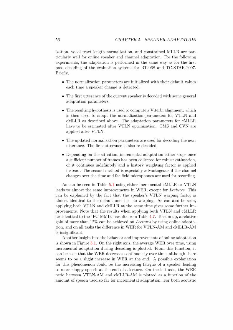
56 CHAPTER 5. SPEAKER ADAPTATION
ization, vocal tract length normalization, and constrained MLLR are par-ticularly well for online speaker and channel adaptation. For the followingexperiments, the adaptation is performed in the same way as for the firstpass decoding of the evaluation systems for RT-06S and TC-STAR-2007.Briefly,
• The normalization parameters are initialized with their default valueseach time a speaker change is detected.
• The first utterance of the current speaker is decoded with some generaladaptation parameters.
• The resulting hypothesis is used to compute a Viterbi alignment, whichis then used to adapt the normalization parameters for VTLN andcMLLR as described above. The adaptation parameters for cMLLRhave to be estimated after VTLN optimization. CMS and CVN areapplied after VTLN.
• The updated normalization parameters are used for decoding the nextutterance. The first utterance is also re-decoded.
• Depending on the situation, incremental adaptation either stops oncea sufficient number of frames has been collected for robust estimation,or it continues indefinitely and a history weighting factor is appliedinstead. The second method is especially advantageous if the channelchanges over the time and far-field microphones are used for recording.
As can be seen in Table 5.1 using either incremental cMLLR or VTLNleads to almost the same improvements in WER, except for Lectures. Thiscan be explained by the fact that the speaker’s VTLN warping factor isalmost identical to the default one, i.e. no warping. As can also be seen,applying both VTLN and cMLLR at the same time gives some further im-provements. Note that the results when applying both VTLN and cMLLRare identical to the “FC-MMIE” results from Table 4.7. To sum up, a relativegain of more than 12% can be achieved on Lectures by using online adapta-tion, and on all tasks the difference in WER for VTLN-AM and cMLLR-AMis insignificant.
Another insight into the behavior and improvements of online adaptationis shown in Figure 5.1. On the right axis, the average WER over time, usingincremental adaptation during decoding is plotted. From this function, itcan be seen that the WER decreases continuously over time, although thereseems to be a slight increase in WER at the end. A possible explanationfor this phenomenon could be the increasing fatigue of a speaker leadingto more sloppy speech at the end of a lecture. On the left axis, the WERratio between VTLN-AM and cMLLR-AM is plotted as a function of theamount of speech used so far for incremental adaptation. For both acoustic

5.3. ONLINE ADAPTATION 57
Dev EvalVTLN-AM cMLLR-AM VTLN-AM cMLLR-AM
RT-06Sno adaptation 33.3% 33.0% 42.1% 42.6%incr. VTLN 28.9% 29.0%incr. cMLLR 29.1% 28.7%both 27.9% 27.7% 35.6% 35.6%
TC-STAR-07no adaptation 20.3% 21.1% 18.3% 18.7%incr. VTLN 16.6% 16.9%incr. cMLLR 16.5% 16.7%both 15.8% 15.7% 14.3% 14.3%
Lecturesno adaptation 16.4% 16.1% 19.9% 19.8%incr. VTLN 15.8% 15.6%incr. cMLLR 14.5% 14.5%both 14.3% 14.1% 15.7% 15.5%
Table 5.1: Comparison of the improvements due to incremental adaptationduring decoding for systems using a VTLN or a cMLLR acoustic model.
models, VTLN and cMLLR parameters were updated incrementally on aper-utterance basis. For ratios smaller than one, VTLN-AM performs betterthan cMLLR-AM and for values grater than one vice versa. It should benoted that a difference of 0.01 in the WER ratio correspond to an absolutedifference of about 0.15 in WER. From the ratio function over all lecturesin lectDev it can be seen that a sufficient amount of speech for adaptationmust be available before cMLLR-AM outperforms VTLN-AM. According tothe figure, this happens at about 10-15 minutes of speech. By analyzing theresults in more detail, it can be seen that this behavior is not true for alllectures. Mostly responsible for this behavior is t012 for which cMLLR-AMis considerably better almost from the very beginning. For all other lectures,this is not the case. Furthermore, it can be observed, that there is a highfluctuation in the ratio when the amount of adaptation data is small.
One might assume that an optimal strategy would be to switch theacoustic models at a specific point of time, i.e. in this case after 10-15minutes. But due to the inconsistent behavior of the lectures in lectDevand due to the insignificant difference of the final WERs for VTLN-AM andcMLLR-AM, no significant improvement could be achieved in this way.
Another strategy is to start each lecture with some pre-computed adap-tation parameters. While this is relatively easy for VTLN, because of thesmaller number of paramters to estimate, it is more complicated for cM-LLR. In this case, a common technique is to cluster the speakers in the

58 CHAPTER 5. SPEAKER ADAPTATION
0.9
0.95
1
1.05
1.1
0 5 10 15 20 25 12
14
16
18
20
22
24
26
28
WER
ratio
bet
ween
VTL
N-AM
and
cMLL
R-AM
WER
duration [min]
VTLN-AM better than cMLLR-AM
cMLLR-AM better than VTLN-AM
WER over time (right axe)WER ratio on all lectures (left axe)
t035l003t032t041t042t012
Figure 5.1: The right axis is for the average WER by using incrementaladaptation plotted as a function of amount of data available for estimatingthe adaptation parameters. The left axis is for the evolution of WER ratiosbetween VTLN-AM and cMLLR-AM as well as a function of the amount ofadaptation data. All results are achieved on lectDev.

5.4. OFFLINE ADAPTATION 59
training data into several classes and to compute for each class adaptationparameters over all speakers in that class. After decoding the first utterance,the resulting hypothesis is used to select the best class. For each class thelikelihoods are computed using a forced Viterbi alignment with the givenhypothesis. After selection, the pre-computed parameters are mixed withthe current estimate using a history weighting factor. For decoding the firstutterance, some default parameters obtained either on the full training dataor on a representative subset can be used. For clustering the speakers of thetraining data, two different techniques were explored (the number of classeswhere determined empirically beforehand to be 25):
• The VTLN parameters were used to cluster all speakers in the trainingdata into 25 classes. For decoding the first utterance, the parametersof the class of the default warping factor of 1.0 were used.
• The similarity between adaptation parameters (i.e. for cMLLR the ro-tation matrix and translation vector) are used to cluster all speakersin the training data into 25 classes. Similar to [MOS06], this was doneby (1) vectorizing for each speaker the rotation matrix by append-ing all matrix columns to the translation vector, (2) normalizing eachdimension over all speakers to have zero mean and unit variance, (3)using principal component analysis to reduce the dimensionality of thevectors, and (4) clustering the vectors of all speakers into 25 classesusing k-means. For the third step, different dimensionality reductionmethods were compared.
When comparing the WER ratio on all lectures between Figure 5.1,where no pre-computed adaptation parameters were used, and Figure 5.2, itcan be seen that for both clustering techniques the performance on the firstfew utterances improved. This is recognizable in the vertical shift of someof the curves towards the top. However, this is not true for all lectures. Butoverall it can be observed that using the similarity of cMLLR parametersas clustering criterion performs better than using VTLN parameters, andcompared to not using any pre-computed adaptation parameters at all, theoverall WER could be reduced by 1.3% on lectDev.
5.4 Offline AdaptationIn contrast to online adaptation, offline speaker adaptation is performed onlyprior to decoding. Therefore, in addition to VTLN and cMLLR, also morecomputationally expensive techniques such as model space MLLR or MAPcan be used. In the following experiments, the improvements obtained usingsupervised or unsupervised adaptation with different amounts of adaptationdata of the same speaker will be analyzed. For this purpose, utterances fromthe lectOther (see Table 4.3) set were randomly selected across the different

60 CHAPTER 5. SPEAKER ADAPTATION
0.9
0.95
1
1.05
1.1
0 5 10 15 20 25 12
14
16
18
20
22
24
26
28
WER
ratio
bet
ween
VTL
N-AM
and
cMLL
R-AM
WER
duration [min]
VTLN-AM better than cMLLR-AM
cMLLR-AM better than VTLN-AM
WER over time (right axe)WER ratio on all lectures (left axe)
t035l003t032t041t042t012
(a) The adaptation parameters were obtained for each cluster after clustering the trainingspeakers according to their VTLN parameters.
0.9
0.95
1
1.05
1.1
0 5 10 15 20 25 12
14
16
18
20
22
24
26
28
WER
ratio
bet
ween
VTL
N-AM
and
cMLL
R-AM
WER
duration [min]
VTLN-AM better than cMLLR-AM
cMLLR-AM better than VTLN-AM
WER over time (right axe)WER ratio on all lectures (left axe)
t035l003t032t041t042t012
(b) The adaptation parameters were obtained for each cluster after clustering the trainingspeakers according to their similarity in cMLLR parameters.
Figure 5.2: Evolution of WER ratios for VTLN-AM and cMLLR-AM onlectDev using pre-computed adaptation parameters.
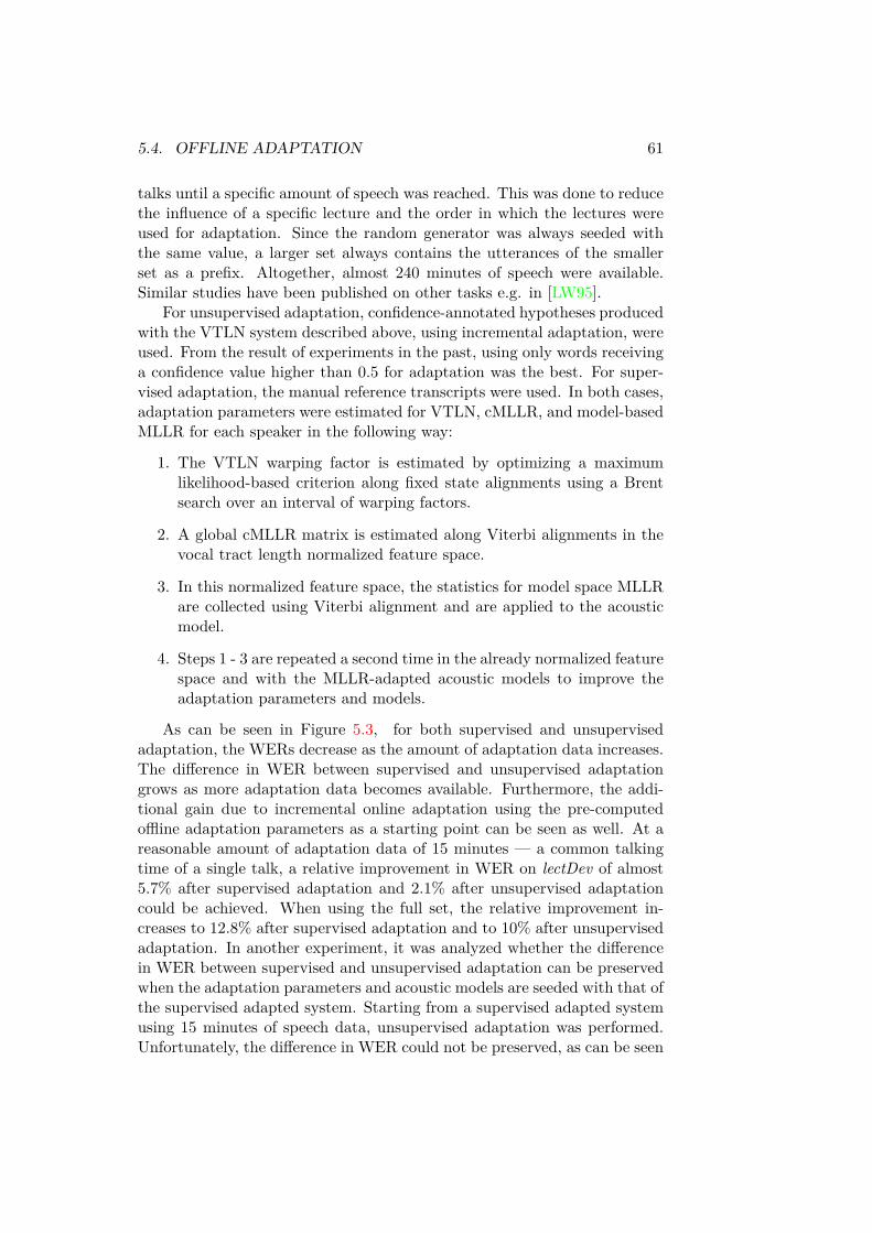
5.4. OFFLINE ADAPTATION 61
talks until a specific amount of speech was reached. This was done to reducethe influence of a specific lecture and the order in which the lectures wereused for adaptation. Since the random generator was always seeded withthe same value, a larger set always contains the utterances of the smallerset as a prefix. Altogether, almost 240 minutes of speech were available.Similar studies have been published on other tasks e.g. in [LW95].
For unsupervised adaptation, confidence-annotated hypotheses producedwith the VTLN system described above, using incremental adaptation, wereused. From the result of experiments in the past, using only words receivinga confidence value higher than 0.5 for adaptation was the best. For super-vised adaptation, the manual reference transcripts were used. In both cases,adaptation parameters were estimated for VTLN, cMLLR, and model-basedMLLR for each speaker in the following way:
1. The VTLN warping factor is estimated by optimizing a maximumlikelihood-based criterion along fixed state alignments using a Brentsearch over an interval of warping factors.
2. A global cMLLR matrix is estimated along Viterbi alignments in thevocal tract length normalized feature space.
3. In this normalized feature space, the statistics for model space MLLRare collected using Viterbi alignment and are applied to the acousticmodel.
4. Steps 1 - 3 are repeated a second time in the already normalized featurespace and with the MLLR-adapted acoustic models to improve theadaptation parameters and models.
As can be seen in Figure 5.3, for both supervised and unsupervisedadaptation, the WERs decrease as the amount of adaptation data increases.The difference in WER between supervised and unsupervised adaptationgrows as more adaptation data becomes available. Furthermore, the addi-tional gain due to incremental online adaptation using the pre-computedoffline adaptation parameters as a starting point can be seen as well. At areasonable amount of adaptation data of 15 minutes — a common talkingtime of a single talk, a relative improvement in WER on lectDev of almost5.7% after supervised adaptation and 2.1% after unsupervised adaptationcould be achieved. When using the full set, the relative improvement in-creases to 12.8% after supervised adaptation and to 10% after unsupervisedadaptation. In another experiment, it was analyzed whether the differencein WER between supervised and unsupervised adaptation can be preservedwhen the adaptation parameters and acoustic models are seeded with that ofthe supervised adapted system. Starting from a supervised adapted systemusing 15 minutes of speech data, unsupervised adaptation was performed.Unfortunately, the difference in WER could not be preserved, as can be seen

62 CHAPTER 5. SPEAKER ADAPTATION
11
12
13
14
15
16
1 2 3 4 5 10 15 30 60 90 120 180 240
WER
amount of adaptation data [min]
baseline incrementalunsupervised fixed
unsupervised incrementalsupervised fixed
supervised incrementalmixed incremental
Figure 5.3: Comparison of supervised and unsupervised adaptation withrespect to the amount of available data. For the curves marked with in-cremental, online adaptation was performed during decoding, while for thecurves marked with fixed the pre-computed offline adaptation parameterswere used instead and no online adaptation was performed. For the mixedcurve, the unsupervised adaptation was seeded with a supervised adaptedsystem.
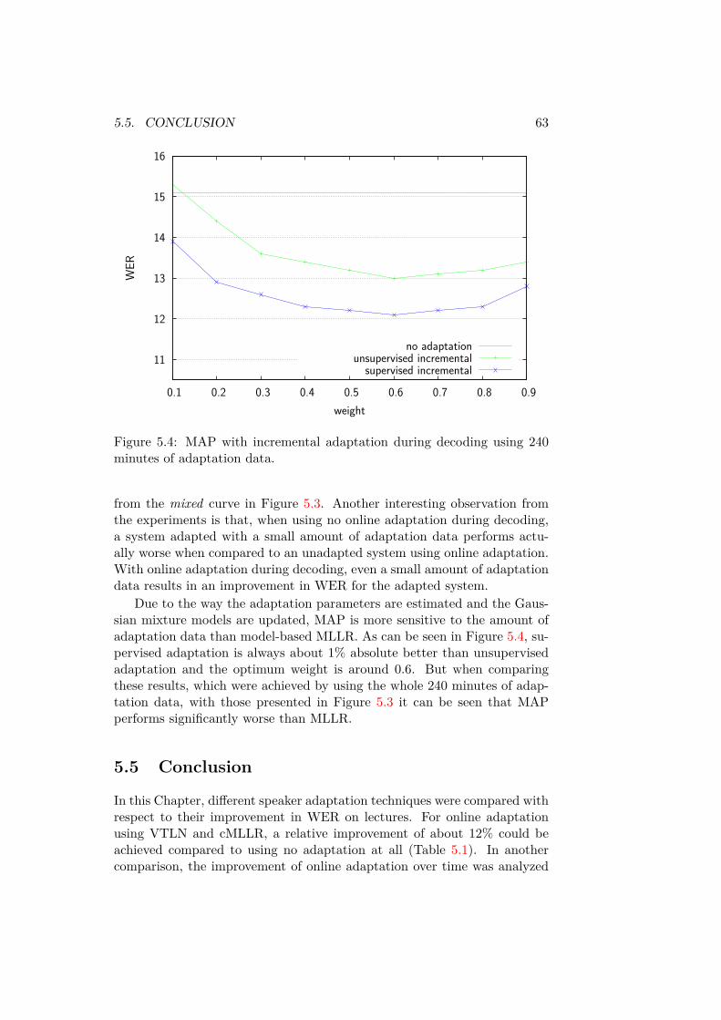
5.5. CONCLUSION 63
11
12
13
14
15
16
0.1 0.2 0.3 0.4 0.5 0.6 0.7 0.8 0.9
WER
weight
no adaptationunsupervised incremental
supervised incremental
Figure 5.4: MAP with incremental adaptation during decoding using 240minutes of adaptation data.
from the mixed curve in Figure 5.3. Another interesting observation fromthe experiments is that, when using no online adaptation during decoding,a system adapted with a small amount of adaptation data performs actu-ally worse when compared to an unadapted system using online adaptation.With online adaptation during decoding, even a small amount of adaptationdata results in an improvement in WER for the adapted system.
Due to the way the adaptation parameters are estimated and the Gaus-sian mixture models are updated, MAP is more sensitive to the amount ofadaptation data than model-based MLLR. As can be seen in Figure 5.4, su-pervised adaptation is always about 1% absolute better than unsupervisedadaptation and the optimum weight is around 0.6. But when comparingthese results, which were achieved by using the whole 240 minutes of adap-tation data, with those presented in Figure 5.3 it can be seen that MAPperforms significantly worse than MLLR.
5.5 Conclusion
In this Chapter, different speaker adaptation techniques were compared withrespect to their improvement in WER on lectures. For online adaptationusing VTLN and cMLLR, a relative improvement of about 12% could beachieved compared to using no adaptation at all (Table 5.1). In anothercomparison, the improvement of online adaptation over time was analyzed

64 CHAPTER 5. SPEAKER ADAPTATION
between a system using an acoustic model trained with VTLN and anotherone trained with cMLLR in addition to VTLN. From Figures 5.1 and 5.2,it was seen how important pre-computed adaptation parameters are, espe-cially for the first few utterances, if a cMLLR trained acoustic model is usedfor decoding. In advance to decoding, a set of adaptation parameters wasobtained by clustering the training speakers, from which appropriate entrieswere selected during decoding. Two different speaker clustering techniqueswere developed, one using VTLN parameters and the other one using thesimilarity between cMLLR parameters. It was shown that significant im-provements on the first few utterances could be achieved for both.
Furthermore, it was shown how available audio data of the same speakercan be used for supervised and unsupervised adaptation using model-basedMLLR (Figure 5.3). In this context, it was shown that the results obtainedwith a supervised adapted acoustic model can also be improved using onlineadaptation. A relative improvement of about 3-5% could be obtained almostindependently of the amount of data used for supervised adaptation. Inaddition, it was seen that the WER can be significantly improved even witha few minutes of data used for supervised or unsupervised adaptation. Arelative improvement of about 5.7% and 7%, for unsupervised and supervisedadaptation, respectively, compared to an unadapted system can be expectedwith about 10-15 minutes of audio data of the same speaker – a commonspeaking time for a talk. When using all available data (almost 4 hours), arelative improvement of 12.8% and 17.7%, for unsupervised and supervisedadaptation, respectively, over the baseline of 14.1% was obtained, i.e. a finalWER of 12.3%, respectively 11.6%.
Figure 5.5 compares the WER improvements due to the different adap-tation techniques and the amount of data used to estimate the adaptationparameters on the evaluation data. Starting with a system using no adap-tation at all, the WER could be reduced by 21% to 15.5% when usingonline adaptation (incr-SA). When 15 minutes of audio data of the samespeaker becomes available, the WER could be further reduced by 4.5% forunsupervised (unsup-incr-15) and by 7.1% for supervised adaptation (sup-incr-15), in addition to online adaptation. Using all available data resultsin an improvement of about 11% for unsupervised and 16% for supervisedadaptation, i.e. a final WER of 13.8%, respectively 13.0%.

5.5. CONCLUSION 65
0
5
10
15
20
25
naa-SAincr-SA
unsup-incr-15
sup-incr-15
unsup-incr-full
sub-incr-full
WER
base20.9
16.2 15.5 15.2 14.613.6
rescored19.7
15.5 14.8 14.4 13.8 13.0
Figure 5.5: Comparison of the different speaker adaptation techniques onthe evaluation data.

66 CHAPTER 5. SPEAKER ADAPTATION
Chapter 6
Topic Adaptation
Depending on the amount of information available prior to simultaneoustranslation, different techniques can be applied to adapt the models of thesystem towards a specific speaker, topic, or even a special talk. Speakeradaptation was already discussed in the preliminary chapter. This chapterwill concentrate on describing the topic adaptation framework. As in theprevious chapters, the descriptions and experiments focus more on the adap-tation of the speech recognition component of the system, i.e. the languagemodel and vocabulary, rather than the translation component. Nevertheless,at the end of this chapter, it is shown that some adaptation techniques caneasily be applied to the target language model in the translation componentas well.
6.1 The Adaptation Framework
Figure 6.1 gives an overview of the adaptation framework developed in thisthesis. This flowchart is processed by the lecture translation system priorto each lecture.
• If neither the lecturer nor the title or topic of a lecture are knownin advance, the system loads general speaker-independent acoustic,language, and translation models.
• If only the name of the speaker is known, and the speaker has alreadygiven a lecture on which the system has adapted its models, the systemis able to load speaker-adapted acoustic models. Since the topic isunknown, it has to load general adapted language and translationmodels. If there is no information about the speaker stored in thedatabase, speaker independent models have to be loaded. In bothcases, the information about the speaker can be used to query theInternet for previously given lectures or other publications by the samespeaker to adapt the language and translation models.
67

68 CHAPTER 6. TOPIC ADAPTATION
Figure 6.1: The adaptation framework. Flow-chart of the different adapta-tion granularities in a lecture translation system.
• If the title or the slides of the talk are additionally available in advance,this information can be used to search the Internet for even morespecific material. Therefore, topic-related keywords or n-grams haveto be extracted from the title or slides.
The more information about a speaker or topic is known in advance, thebetter the models can be adapted and the better the system might performultimately. The information can either be given manually or retrieved au-tomatically from the Internet. For adaptation, the material collected mustfirst be filtered and normalized in order to interpolate it with the othermore general background models. Although not shown in the figure, it alsomakes sense to adapt the vocabulary of the speech recognizer by extendingit with missing topic words or proper names. Section 6.4 deals with thisissue separately. The next Section describes techniques for language modeladaptation.
6.2 Language Model AdaptationThe main adaptation technique used is the so-called model interpolation,in which several language model components LMi are linearly interpolatedto form a mixture model. The probability for a word w following the wordhistory h is then computed as follows:
P (w|h) =∑LMi
λiPi(w|h), with∑i
λi = 1 (6.1)
The mixture coefficients or interpolation weights λi may be a function ofthe word history h and are typically estimated with the help of the EM al-
6.2. LANGUAGE MODEL ADAPTATION 69
gorithm so that the perplexity of the mixture model on some held-out datais optimized. Language model adaptation is performed by updating the in-terpolation weights with the help of additional held-out data and/ or byexchanging or adding some language model components which better coverthe desired topics. Adding new components can be done either by interpo-lating them with the already existing language model, or by re-estimatingall mixture coefficients. While in the first case the existing (background)language model is kept unchanged, in the second case the interpolated lan-guage model has to be computed from scratch. The first method is preferredbecause of its smaller computationally effort, and used for most of the exper-iments in this thesis, but as will be seen later, better results can be obtainedby using the second approach.
Other techniques used for language model adaptation include dynamiccache language models [KdM90], minimum discriminant information (MDI)[Fed99], or latent semantic analysis (LSA) [Bel00], but are not further in-vestigated in this thesis. A more detailed overview of statistical languagemodel adaptation techniques can be found in the journal article by Belle-garda [Bel04].
6.2.1 Useful Data for Adaptation
But what kind of data is useful for adaptation and where can that data beobtained? This section deals with these two questions and describes theproblems and advantages of different types of data.
Manual or Automatic Transcripts
The best data for language modeling for speech recognition are transcripts ofspeech data. This data is preferred over text data because spoken languagediffers in style from text, due to spontaneous effects like word reorderings,word repetitions, breaks, hesitations and other disfluencies. Since speechrecognizers have to recognize word-by-word, well-estimated transitions cov-ering these kinds of disfluencies are essential.
Transcribing speech data can be done manually, or automatically if agood enough speech recognition system is available. Initially during systemdevelopment, this is not the case, and, due to recognition errors manualtranscripts are usually preferred over automatic ones. On the other hand,manually transcribing data is very costly and many occurrences of disflu-encies further complicate this process. Therefore, different approaches tospontaneous language modeling have already been investigated in the liter-ature. A good introduction to the problem can be found in the article byStouten [SDMW06].
Often, the estimation of the probabilities for inserting disfluencies istreated separately from statistical n-gram language modeling. For example,

70 CHAPTER 6. TOPIC ADAPTATION
in [SS96], a so-called hidden event language model was used. In [HWM03], aweighted finite state transducer for speaking style translation was proposedinstead. However, the success of such approaches, in comparison to modelingthem directly in the n-gram language model, depends on the transcribedspontaneous speech already available.
The recognition system used in this thesis models some disfluencies, suchas word repetitions or breaks, directly, with the help of the language model.In contrast, so-called filler words which are allowed to occur between anyother two regular words are handled differently. Their language model prob-abilities are not computed by the language model. Instead, a fixed fillerpenalty optimized on some held-out data is used. The category of fillerwords covers hesitations as well as human and non-human noises.
Topic-Related Text Data
For topic adaptation, data related to a particular topic is necessary. Again,transcripts are preferred over text data, but are more difficult to find thanspontaneous speech transcripts. In the literature, one can distinguish be-tween approaches for selecting data related to a particular topic out of alarge corpus [MBH99], approaches for further collecting related text data byquerying a search engine and retrieving resulting web pages from the WorldWide Web [BOS03, WH06, SGN05], or a combination of both. Using thehuge amount of data available in the Internet has increased in popularityover the last years because of the higher quality of search engines. Writ-ten data which is similar to spontaneous speech can be found in many chatrooms [BOS03].
As already introduced during the explanation of the adaptation frame-work, the approach used in this thesis is to query the Internet. Therefore,queries have to be generated for retrieving relevant documents by using websearch engines.
6.2.2 Query Generation using TF-IDF
The procedure for query generation presented here was developed for theRT-06S evaluation. For web text collections used for training the LM6language model, two different web query strategies were employed. For theUKA-L collection, the same web text collection framework as proposed in[BOS03] was followed, where frequently spoken 3-grams and 4-grams fromthe target task training data are combined to form queries. For the othercollections, a more sophisticated approach was used. Frequent n-grams fromdifferent lecture or conference meeting transcripts were combined with topicbigrams from the conference proceedings PROC to form queries. The goalwas to obtain text reflecting a broad variety of topics, some of which are notrepresented in the training set, as well as data covering the desired speaking
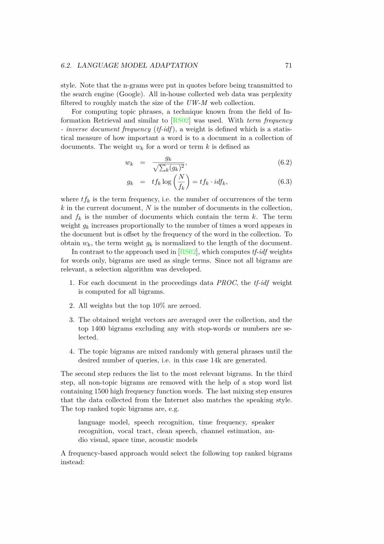
6.2. LANGUAGE MODEL ADAPTATION 71
style. Note that the n-grams were put in quotes before being transmitted tothe search engine (Google). All in-house collected web data was perplexityfiltered to roughly match the size of the UW-M web collection.
For computing topic phrases, a technique known from the field of In-formation Retrieval and similar to [RS02] was used. With term frequency- inverse document frequency (tf-idf ), a weight is defined which is a statis-tical measure of how important a word is to a document in a collection ofdocuments. The weight wk for a word or term k is defined as
wk = gk√∑k(gk)2
, (6.2)
gk = tfk log(N
fk
)= tfk · idfk, (6.3)
where tfk is the term frequency, i.e. the number of occurrences of the termk in the current document, N is the number of documents in the collection,and fk is the number of documents which contain the term k. The termweight gk increases proportionally to the number of times a word appears inthe document but is offset by the frequency of the word in the collection. Toobtain wk, the term weight gk is normalized to the length of the document.
In contrast to the approach used in [RS02], which computes tf-idf weightsfor words only, bigrams are used as single terms. Since not all bigrams arerelevant, a selection algorithm was developed.
1. For each document in the proceedings data PROC, the tf-idf weightis computed for all bigrams.
2. All weights but the top 10% are zeroed.
3. The obtained weight vectors are averaged over the collection, and thetop 1400 bigrams excluding any with stop-words or numbers are se-lected.
4. The topic bigrams are mixed randomly with general phrases until thedesired number of queries, i.e. in this case 14k are generated.
The second step reduces the list to the most relevant bigrams. In the thirdstep, all non-topic bigrams are removed with the help of a stop word listcontaining 1500 high frequency function words. The last mixing step ensuresthat the data collected from the Internet also matches the speaking style.The top ranked topic bigrams are, e.g.
language model, speech recognition, time frequency, speakerrecognition, vocal tract, clean speech, channel estimation, au-dio visual, space time, acoustic models
A frequency-based approach would select the following top ranked bigramsinstead:

72 CHAPTER 6. TOPIC ADAPTATION
language model, speech recognition, error rate, acoustic models,natural language, proposed method, training data, clean speech,acoustic model, broadcast news
While some of the bigrams between both approaches are identical, it canbe seen that by using tf-idf more specialized bigrams are preferred over themore general ones.
For the adaptation framework, the topic information has to be extractedfor a single talk only, instead of a collection of documents. However, tf-idf weights can only be computed with respect to a collection of docu-ments. Therefore, the data from which the components for the baseline(background) language model were built is used as a background corpus.
The above-presented algorithm has the problem that for some n-grams,tf-idf weights could not be computed because the corresponding n-gramin the background corpus was missing. Furthermore, the hard thresholdsdefined in the selection algorithm makes it unsuitable for changing datasizes. Therefore, the selection algorithm has to be further refined, and,instead of bigrams only, also trigrams were considered. Given some datarelated to the current talk, like presentation slides or publications the topicn-grams are selected according to the following heuristic:
1. Compute bigram and trigram tf-idf weights on the relevant data withrespect to the background corpus.
2. All n-grams with a weight higher than 10% of the highest weight areselected.
3. In addition, all n-grams with no tf-idf weight and a higher occurrencecount than the square of the average occurrence n-gram count areselected.
The count and tf-idf thresholds are defined for each n-gram category sepa-rately.
6.3 Language Model Adaptation ExperimentsIn the following experiments, the different adaptation levels of the proposedadaptation framework are evaluated with respect to improvements in speechrecognition.
In Section 6.3.1, a detailed description of differently adapted languagemodels used as baseline language models for the following experiments aregiven. Section 6.3.2 analyzes to which extent the language model can beadapted, if the speaker’s identity is known. Therefore, the homepage of thespeaker as well as the speaker’s publications are retrieved from the web. InSection 6.3.3, this data was used to retrieve other related data, similar intopic, and the relevance of this data is analyzed in more detail.

6.3. LANGUAGE MODEL ADAPTATION EXPERIMENTS 73
So far, only data related to the interests of the speaker was collected.In the next step, it was analyzed if the adaptation could be improved bydata related to the talk or lecture the speaker is given. Therefore, in Section6.3.4, information on the presentation slides was used to retrieve relevantdata from the web, and the results when using this data for language modeladaptation prior to decoding are presented.
Sections 6.3.5 and 6.3.6 analyzes the improvements possible if more datafrom the speaker becomes available such as recorded lectures. Dependingon the type of the transcripts available, manually transcribed or automatic,the improvements in WER by using this data for LM adaptation is studied.
6.3.1 Baseline Language Models
We analyze in more detail the language model used for the baseline ASR sys-tem. As described in Section 4.3.6, this language model (LM6) is a mixturelanguage model consisting of nine different language model components; itevolved over several evaluations [FKPW06, FIK+06]. The main improve-ments were made prior to the RT-06S evaluation when a huge amount ofadditional data was collected from the Internet with the technique describedin Section 6.2.2.
For the experiments within this chapter, LM6 was modified to betterhandle disfluencies. As described above, instead of estimating their transi-tion probabilities by the language model, a fixed penalty was used instead.This was done for only those disfluencies which seem to occur independentlyfrom their surrounding word context. As a result, the perplexities as wellas the WERs given in this chapter differ from those presented in Section4.3. Due to this change, the PPL improves by 17% on RT-06Sdev and 8%on lectDev, and the WER improved by 3.2% and 2.8%, respectively. Theimprovement is not only because of the changed modeling; the penalty ap-plied is also much smaller than compared to the average language modelprobability estimate of a disfluency transition in LM6, making it more likelyfor disfluencies to be recognized. The same normalization was applied toall other LMs in this chapter. It should be noted that, throughout all lan-guage model adaptation experiments, the language model vocabulary waskept fixed to the one described in Section 4.3.5.
Figure 6.2 shows the mixture coefficients for LM6, and Table 6.1 gives thecorresponding perplexities and word error rates on different development andevaluation sets. For LM6, the mixture coefficients were tuned on a held-outset related to the RT-06S evaluation and different from the development andevaluation sets. As can be seen, the most relevant data are the transcripts ofrecorded seminars SMNR, followed by the proceedings data. The fact thatthe proceedings data are only second in importance shows the technicalrelatedness of the held-out data.
As mentioned above, due to the use of language model components built

74 CHAPTER 6. TOPIC ADAPTATION
Figure 6.2: Mixture coefficients of the training corpora tuned on differentdevelopment sets. Components for which the coefficients are smaller than0.2 are not shown in the figure and also not used for the estimation of theinterpolated LM.
RT-06Sdev lectDevPPL WER PPL WER
LM6 127 27.0% 150 13.9%rt06Sbase 136 28.2% 162 14.5%rt06Sdev 124 26.9% 145lectDev 127 144 13.5%
Table 6.1: In- and across-domain perplexity (PPL) and word error rate(WER) comparison of mixture LMs. rt06Sbase was tuned on RT-06S held-out data, lectBase on the held-out set lectOther, and rt06Sdev and lectDevon the corresponding development sets instead.

6.3. LANGUAGE MODEL ADAPTATION EXPERIMENTS 75
from proceedings data, as well as from large amounts of web data relatedto technical presentations, LM6 is already highly adapted towards the lec-tures which are considered in this thesis. As a result of this, the potentialof the developed adaptation framework is hard to assess because obtainedimprovements on top of the results achieved with LM6 – if any – are rathersmall. To overcome this problem, a new unadapted baseline language modelrt06Sbase was created, for which the allowed corpora were restricted to allaudio transcripts, as well as the text data not collected in the context ofRT-06S, i.e. UW-M, HNSRD, GWRD, UN, and BN. As a held-out setfor computing the mixture coefficients, the RT-06S held-out data was used.This corresponds to the realistic situation of applying the lecture translationsystem, for the first time for a specific speaker and a particular topic, giventhat the system had been already used in a similar situation for anotherspeaker. Besides some related transcripts and additional held-out data, noother corresponding data is available.
As can be seen in Figure 6.2, the most relevant corpora for rt06Sbase areUW-M, SMNR, MTG, and TED. And Table 6.1 shows that on RT-06Sdev, aperplexity of 136, and 162 on lectDev can be achieved. The WERs obtainedon RT-06Sdev and lectDev are 28.2%% and 14.5%, respectively.
For comparison reasons two other language models were created. Thert06Sdev language model was tuned with respect to the RT-06Sdev data,and the lectDev language model with respect to the lectDev data, ratherthan with respect to the corresponding held-out data sets. Compared toLM6, some differences can be observed. The proportions between differentcomponents are modified, the TED language model is not important any-more, and the EPPS-S language model is added with a small weight. Whilefor rt06Sdev the meeting transcripts are the most important, for lectDev theweb data based on meeting transcripts and proceedings is the most relevant.Due to this difference, the perplexities on the corresponding data set are alsoreduced by 3 and 6 for RT-06Sdev and lectDev respectively, relative to LM6.Only a slight WER reduction for rt06Sdev of 0.4% to a WER of 13.5% wasobserved.
The language models lectBase and lectAdapt will be described later inSection 6.3.5. To reduce the size in memory, all language models were prunedwith an entropy-based criterion using a threshold of 10−9 [Sto98].
6.3.2 Using the Speaker’s Identity
With the help of the speaker’s identity, the Internet can be queried foradditional information about the speaker. Ideally, the homepage, along withthe speaker’s publications can be found. Although querying a search enginewith the speaker’s name is possible, a better method is to search manuallyfor the necessary information, since the name might not be unique. If thehomepage is found, a web crawler can be used to retrieve the necessary

76 CHAPTER 6. TOPIC ADAPTATION
pages recursively, i.e. together with linked pages up to a specified linkingdepth. All the found pages as well as the publications can now be filtered,normalized and merged. Note that for this adaptation level, no topic n-grams have to be extracted.
Filtering removes unnecessary information such as HTML code, tables,formulas, special characters, etc. After this, sentence boundaries or para-graphs are detected. Additional filters are applied to remove sentences,paragraphs or documents if they have a worse ratio of real words to out-of-vocabulary words, of numbers to words, or of number of characters to words.Out-of-vocabulary words are identified with the help of a large backgroundvocabulary with about 500k entries. The normalization step writes out ab-breviations and numbers, tags acronyms, and removes punctuation. Thenormalized pages and documents can now be merged into a single corpus.
Experiments
The following experiments were conducted on the lecture task as well as onthe RT-06S data. Due to the lack of held-out and evaluation data with addi-tional speaker information, it was necessary to partition the RT-06Sdev setrandomly into a development (RT-06Sdev-dev) and evaluation (RT-06Sdev-eval) set. All word error rates are given after language model rescoring, withthe language model parameters optimized on the development data.
Data: Table 6.2 gives an overview of the amount of data collected perspeaker as well as the adaptation results. As mentioned above, rt06Sbase wasused as a baseline, and as the background language model for interpolationwith the foreground language models built from the data collected. Sincesome of the speakers are students, no additional information or publicationswere found about them on the Internet, and the data found about theirsupervisor was used instead. As a result, for two speakers with the IDsevsmbd and robdkz, as well as for the two speakers pgaftk and qgzhyn, thesame data is used. As can be seen in the second column of Table 6.2, theamount of data found per speaker varies largely from about 3k to 555k.
The relevance of the collected data: For measuring the relevance ofthe collected data with respect to different speakers, a language model buildon a speaker’s data only. The perplexities were computed on all speakers’reference transcripts of the development set and compared. Table 6.3 showsthe results. As can be seen, the perplexities for the matched condition areusually amongst the top two lowest for a single speaker. This is not thecase for only those speakers for which the data used is identical to that ofanother speaker, and for evsmbd. An analysis of the transcripts for evsmbdshows that this speaker employs more general language than others.

6.3. LANGUAGE MODEL ADAPTATION EXPERIMENTS 77
speaker ID # words PPL-b WER-b weight PPL-i WER-iRT-06Sdev development set
bpdnpq 17,409 165 28.6% 0.27 118 25.1%evsmbd 155,378 101 14.9% 0.14 97 13.4%ksb 425,853 154 24.7% 0.33 124 23.8%mlspsf 3,280 103 21.0% 0.05 101 20.4%ouarkw 234,014 119 28.2% 0.17 110 26.8%pgaftk 5,100 132 25.6% 0.02 132 25.9%qgzhyn 5,100 157 23.3% 0.09 145 24.1%robdkz 155,378 117 30.3% 0.10 104 29.5%spipaa 201,074 182 22.4% 0.37 141 20.0%Overall 1,202,586 135 25.1% 0.17 122 24.2%+ threshold 0.23 24.0%
RT-06Sdev evaluation setjjabpr 155,378 166 41.3% 0.17 40.5%kesysg 188,524 143 29.0% 0.17 27.7%kuvvqe 336,840 137 44.7% 0.17 42.8%ojtlvn 2,925 157 25.6% 0.17 26.5%owm 555,209 130 23.6% 0.17 22.5%pgv 103,269 124 23.4% 0.17 22.3%ristxa 74,375 123 26.5% 0.17 27.2%tbvstt 5,344 126 32.2% 0.17 32.1%xboxkz 20,468 129 29.8% 0.17 29.6%Overall 1,442,332 30.3% 0.17 30.0%+ threshold 0.23 29.9%
Table 6.2: Amount of data collected per each speaker on the RT-06Sdevset together with the mixture weights and resulting perplexities (PPL) andword error rates (WER). PPL-b and WER-b are the results computed withthe baseline language model rt06Sbase, and PPL-i and WER-i are the resultsafter language model adaptation using the collected data. WERs are givenafter language model rescoring.
data\ref bpdnpq evsmbd ksb mlspsf ouarkw pgaftk qgzhyn robdkz spipaabpdnpq 440 584 1794 1486 1562 2242 1892 1342 2068evsmbd 406 320 1030 904 987 1480 1209 1132 1284ksb 629 184 234 368 572 694 528 769 649mlspsf 2096 1166 2264 1029 2995 3001 2837 3205 3461ouarkw 322 179 596 539 450 1023 712 772 782pgaftk 2902 1399 2436 1752 3482 2569 1480 4142 3495qgzhyn 2902 1399 2436 1752 3482 2569 1480 4142 3495robdkz 406 320 1030 904 987 1480 1209 1132 1284spipaa 654 242 459 335 467 604 545 572 258
Table 6.3: Perplexities of different speaker’s data on different speaker’s ref-erence transcripts restricted to RT-06S-dev-dev. In bold, the two lowestperplexities per row are marked.

78 CHAPTER 6. TOPIC ADAPTATION
It could be shown, that the data retrieved for a specific speaker is corre-lated in terms of perplexity with the presentation of the speaker. In the nexttwo experiments it is analyzed, if this relationship carries over to improve-ments in WER. In the first experiment (A), lecture meetings are explored,and in the second experiment (B), lectures.
(A) Lecture meetings: In the third and fourth column of Table 6.2, theperplexities (PPL-b) and word error rates (WER-b) achieved with the base-line language model are given. Overall, a perplexity of 135 together with aWER of 25.1% is obtained on the development set. For each speaker, thelanguage model component built on the speaker’s collected data is interpo-lated with the background language model. The optimized mixture weightsobtained on the speaker’s reference transcripts are given in the fifth column(weight), and the resulting perplexity on the same references in the sixthcolumn (PPL-i). Due to the fact that speaker-dependent mixture weightscannot be estimated on the evaluation set, a single average mixture weightwas computed. For the decoding experiments, this weight was used forthe interpolation of the language model components for all speakers. Thismeans that the word error rates given in the last column are obtained withthe speaker adapted mixture models using a weight of 0.17 for the fore-ground language model component. As can be seen, the overall baselineWER can be improved by 3.5% to 24.2% on the development set. Althoughthe improvement is not as large as on the development set, an improvementfrom 30.3% down to 30.0% could also be observed on the evaluation data.Another observation is that the adaptation typically works better for speak-ers for whom more data is available. Therefore, the result can be furtherimproved slightly when the speaker-adapted language model is used onlyif the collected data amounts to more than e.g. 10,000 words. The WERcould be improved to 24.0% on the development set and to 29.9% on theevaluation set.
Unfortunately, the random partition of the RT-06Sdev speakers into thetwo sets was not ideal. The development set is much easier to recognize thanthe evaluation set. Moreover, the mixture weights obtained on the develop-ment set are overestimated compared to those which would be achieved onthe evaluation set. The average optimal weight on the evaluation set is 0.14– much lower than the computed 0.23.
(B) Lectures: The above-described adaptation strategy was also appliedto the lecture task. Since all data was recorded from a single speaker asingle corpus with an amount of 607,097 words was collected. The languagemodel component built on this data was then interpolated with a weightof 0.15 with the background language model rt06Sbase, with the mixturecoefficient optimized on RT-06Sdev-dev. As can be seen in Table 6.4, the

6.3. LANGUAGE MODEL ADAPTATION EXPERIMENTS 79
ID PPL-b WER-b PPL-i WER-i WER-b’ WER-i’t035 164 14.7% 152 14.5% 14.7% 14.3%l003 154 14.6% 150 14.3% 14.5% 14.3%t012 168 17.4% 156 17.1% 17.3% 17.1%t032 148 12.6% 142 12.4% 12.5% 12.3%t041 196 14.3% 194 14.6% 14.2% 14.3%t042 192 12.1% 175 12.5% 12.1% 12.1%Overall 162 14.5% 156 14.3%
Table 6.4: Word error rates and perplexities on lectDev before and afterlanguage model adaptation. While WER-b and WER-i are those obtainedwith the global best language model parameters,WER-b’ andWER-i’ showsthe word error rates with the local best language model parameters. Themixture coefficient was optimized on the above introduced RT-06Sdev de-velopment set to 0.15.
overall perplexity was reduced from 162 (PPL-b) to 156 (PPL-i), and theword error rate from 14.5% (WER-b) to 14.3% (WER-i). However, thisreduction is not obtainable for all lectures. Although the perplexity wasreduced for all lectures, the word error rate for t041 and t042 increased.The reason for this behavior is due to the way in which the results afterlanguage model rescoring are obtained. The WERs presented in the WER-icolumn are those achieved with the language model parameters achievingthe overall best WER. However, these language model parameters might notbe optimal for all lectures. Therefore, in the WER-b’ and WER-i’ columns,the WERs achieved with the best language model parameters per lectureare given. As can be seen, these WERs correlate better with the presentedperplexities. However, unless otherwise specified, the tables which followgive only WER-b and WER-i.
Conclusion
In this Section, it was shown that data retrieved from the homepage of aspeaker together with the speaker’s publications contains useful informationrelevant to a speaker’s presentation. Using this data for language modeladaptation by linear interpolation with a background language model im-proves perplexity as well as word error rate. On lecture meetings, the WERcould be improved by 3.5% and 1% relative on the development and eval-uation data, respectively. On lectures, the WER could be improved from14.5% to 14.3%. Although consistent, the improvements are relatively small.Therefore, the next section investigates, if the results can be improved, ifthis data is used as a seed corpus for collecting additional data.
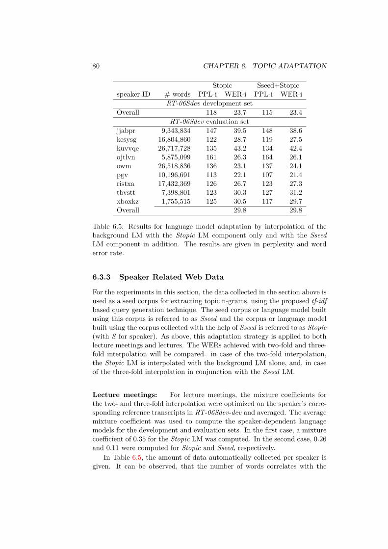
80 CHAPTER 6. TOPIC ADAPTATION
Stopic Sseed+Stopicspeaker ID # words PPL-i WER-i PPL-i WER-i
RT-06Sdev development setOverall 118 23.7 115 23.4
RT-06Sdev evaluation setjjabpr 9,343,834 147 39.5 148 38.6kesysg 16,804,860 122 28.7 119 27.5kuvvqe 26,717,728 135 43.2 134 42.4ojtlvn 5,875,099 161 26.3 164 26.1owm 26,518,836 136 23.1 137 24.1pgv 10,196,691 113 22.1 107 21.4ristxa 17,432,369 126 26.7 123 27.3tbvstt 7,398,801 123 30.3 127 31.2xboxkz 1,755,515 125 30.5 117 29.7Overall 29.8 29.8
Table 6.5: Results for language model adaptation by interpolation of thebackground LM with the Stopic LM component only and with the SseedLM component in addition. The results are given in perplexity and worderror rate.
6.3.3 Speaker Related Web Data
For the experiments in this section, the data collected in the section above isused as a seed corpus for extracting topic n-grams, using the proposed tf-idfbased query generation technique. The seed corpus or language model builtusing this corpus is referred to as Sseed and the corpus or language modelbuilt using the corpus collected with the help of Sseed is referred to as Stopic(with S for speaker). As above, this adaptation strategy is applied to bothlecture meetings and lectures. The WERs achieved with two-fold and three-fold interpolation will be compared. in case of the two-fold interpolation,the Stopic LM is interpolated with the background LM alone, and, in caseof the three-fold interpolation in conjunction with the Sseed LM.
Lecture meetings: For lecture meetings, the mixture coefficients forthe two- and three-fold interpolation were optimized on the speaker’s corre-sponding reference transcripts in RT-06Sdev-dev and averaged. The averagemixture coefficient was used to compute the speaker-dependent languagemodels for the development and evaluation sets. In the first case, a mixturecoefficient of 0.35 for the Stopic LM was computed. In the second case, 0.26and 0.11 were computed for Stopic and Sseed, respectively.
In Table 6.5, the amount of data automatically collected per speaker isgiven. It can be observed, that the number of words correlates with the

6.3. LANGUAGE MODEL ADAPTATION EXPERIMENTS 81
number of words in the Sseed corpus, because the number of queries gener-ated automatically depends on the size of the Sseed corpus. Furthermore,compared to Table 6.2, the perplexity and word error rate can be furtherreduced on the development set. On the evaluation set, the WER decreasesonly slightly for the two-fold interpolation with the Stopic LM to 29.8%,but no further when the Sseed LM is added. A correlation of the numbersof words collected and the WER achieved as compared to Table 6.2 was notobserved.
Lectures: When using the same technique for the lectures an amount of34,116,715 words was collected for the single speaker. Bigrams and trigramswere extracted from the Sseed corpus as search queries for the Stopic corpus.Altogether, 1242 bigrams and 1922 trigrams were extracted. The top rankedbigrams are:
user registration, n-best lists, n-gram language, hand color,speech-to-speech translation, Toolkit JRTk, CallHome Spanish,human-robot interaction, speaker initiative, human-human com-munication, close-talking microphone, cross-language transfer
while the top-ranked trigrams are:
Recognition Toolkit JRTk, GE EN JA, EN JA SP, CH GE EN,n-gram language models, discriminant analysis LDA, multimodaluser registration, n-gram language model, vectorized nontermi-nal symbols, machine translation SMT, hand color model
As can be seen, several specialized n-grams are mixed with general ones.The n-grams similar to “GE EN JA” are common abbreviations for languagepairs in machine translation. But also the lowest ranked n-grams seem tobe relevant, as can be seen in the following trigrams:
speech recognition error, extract signs robustly, recognition errorrates, Ibis single pass, distant microphone conditions, bilingualBasic Travel, individual person activity, global STC transforms,Language Adaptive Acoustic, Sixth Framework Programme
The mixture coefficients were again optimized on the RT-06Sdev-devdevelopment corpus. For the two-fold interpolation of the background LMwith the Stopic LM, a coefficient of 0.31 for the Stopic was obtained, and,after additionally applying the Sseed LM, 0.08 and 0.24 for the Sseed andStopic LM, respectively.
Conclusion
In this section, the Sseed corpus was used as a seed corpus for extractingtopic n-grams, using the proposed tf-idf based query generation technique.

82 CHAPTER 6. TOPIC ADAPTATION
Stopic Sseed+StopicID PPL-i WER-i PPL-i WER-it035 147 14.5% 144 14.6%l003 147 14.3% 145 14.4%t012 156 17.1% 152 16.6%t032 137 12.4% 136 12.1%t041 181 14.6% 181 14.1%t042 163 12.5% 160 11.9%Overall 154 14.2% 151 14.1%
Table 6.6: Word error rates and perplexities on lectDev obtained with lan-guage models adapted by interpolation with the Stopic LM and with theSseed LM in addition.
The resulting queries were used for retrieving additional data forming theStopic corpus. Compared to the results of Section 6.3.2 perplexities as well asword error rates improved further when both corpora, Sseed and Stopic wereused for a three-fold interpolation with the background language model lect-Base. Compared to results obtained with the background language model,the WER was improved by 1.7% and 2.8% on lecture meetings and lectures,respectively.
So far, the experiments focused on general data related to the speakerand was not specific to a presentation. In the following section, it will beinvestigated, if data specific to a presentation can be retrieved from the webby using information extracted from the presentation slides.
6.3.4 Using Presentation Slides
In this section, additional information about the presentation is used forcollecting data from the Internet. Examples of suitable information includepresentation slides or manuscripts. Unfortunately, additional information inthe form of presentation slides was not available for the RT-06S data; thefollowing experiments were therefore carried out on the lecture data only.
As in Section 6.3.2, after describing the collected data per lecture inmore detail, its relevance for the corresponding lecture is shown. The ex-periments are following afterwards. It will be investigated if (A) relevantdata can be collected with the proposed tf-idf based query generation andweb data collection strategy, (B) perplexities as well as word error rates im-prove when this data is used in conjunction with Stopic, and (C) by mergingthis topic-specific data into a single corpus to increase its relevance, furtherimprovements can be achieved.

6.3. LANGUAGE MODEL ADAPTATION EXPERIMENTS 83
ID # bigrams # trigrams # wordst035 221 88 5,957,056l003 1150 388 24,266,155t012 237 72 6,055,540t032 317 433 9,943,847t041 166 145 5,387,185t042 324 174 10,438,130
Table 6.7: Number of queries extracted automatically from the presentationslides together with the number words collected per lecture on lectDev.
Ltopic Stopic+LtopicID PPL-i WER-i PPL-i WER-it035 154 14.6% 146 14.7%l003 144 14.2% 144 14.4%t012 164 17.3% 156 16.7%t032 140 12.3% 137 12.2%t041 178 13.8% 179 13.7%t042 174 12.0% 163 11.9%Overall 14.2% 14.1%
Table 6.8: Results achieved with language model adaptation using web datacollected from presentation slides on lectDev. The mixture coefficients wereoptimized on the RT-06Sdev development set.
Data: Table 6.7 shows the number of queries extracted from the presenta-tion slides and the amount of data collected from these queries per lecture.Again, the amount of data collected depends on the number of queries ex-tracted. The language model or corpus extracted in this way is referred toas Ltopic (with L for lecture dependent).
(A) The relevance of the collected data: To verify the relevance of thecollected data with respect to the different lectures, Table 6.9 compares theperplexities of different topic data collected for a specific lecture computedon different reference transcripts. Except for t012 and t041, the correspond-ing reference transcripts can be found under the two lowest perplexities. Incomparison with the Stopic data, it can be seen that the perplexity is notalways lower.
In summary, the tf-idf -based query generation and web data collectionstrategy collects relevant data, with the relevance increasing as the corpusgrows in size. The data retrieved for a specific lecture is correlated in terms ofperplexity with the lectures reference transcripts. However, a large speaker-dependent corpus, general in topic (Stopic) may be often more suitable

84 CHAPTER 6. TOPIC ADAPTATION
data\ref t035 l003 t012 t032 t041 t042t035 203 296 258 210 243 240l003 201 199 229 182 260 221t012 230 265 262 214 271 260t032 195 259 234 186 235 196t041 210 296 266 218 222 240t042 219 356 281 220 255 203Stopic 188 202 212 176 238 197
Table 6.9: Perplexities of different Ltopic data collected for a specific lectureon different reference transcripts. In addition, the perplexity of the Ltopicdata is compared with the Stopic data. In bold, the two lowest perplexitiesare marked per lecture or talk (row). For Stopic, the perplexity is markedbold if it is lower than the corresponding Ltopic perplexity.
especially if the topic dependent corpus (Ltopic) is relatively small.In the next two experiments it is analyzed, if this relationship carries over
to improvements in WER. In the first experiment (A) presentation specificdata will be used, in the second experiment (B) the presentation specificdata will be merged to a single corpus.
(B) Presentation specific data: For each Ltopic component, the mix-ture coefficients were optimized on the RT-06Sdev-dev set, separately. Themixture coefficient for Ltopic in the case of two-fold interpolation rangesfrom 0.06 to 0.12, and if the Stopic LM is used additionally, from 0.006 to0.01. In terms of WER, no further improvement was achieved compared tothe results presented in Table 6.6. For two-fold interpolation, a WER of14.2% was achieved, for three-fold interpolation the WER was 14.1% (seeTable 6.8). However, although the mixture coefficients are small, the WERsfor the two-fold interpolations with Stopic or Ltopic are identical, showingthat both corpora are relevant. Again, no correlation between the size ofthe Ltopic corpus and WER was observed.
(C) General presentation data: It was observed on Table 6.9 thatsometimes the large speaker-dependent corpus, general in topic Stopic wasmore relevant in terms of perplexity than the more specific, topic-dependentcorpora. Therefore, in this experiment it was investigated, if the relevanceof the Ltopic corpora could be increased as well when merged into a singlecorpus.
After removing duplicate web pages, this corpus consists of 48,726,560words. Again, the mixture coefficients for the two-fold and three-fold in-terpolation with Stopic were optimized on the RT-06Sdev-dev set, withrt06Sbase serving as a background LM. The results in Table 6.10 show a

6.3. LANGUAGE MODEL ADAPTATION EXPERIMENTS 85
Ltopic Stopic+LtopicID PPL-i WER-i PPL-i WER-it035 148 14.0% 145 14.6%l003 148 14.2% 145 14.3%t012 159 16.9% 155 16.6%t032 138 11.9% 136 12.1%t041 173 13.5% 175 13.2%t042 167 11.3% 162 11.9%Overall 154 13.9% 152 14.0%
Table 6.10: Results achieved with language model adaptation using webdata collected from presentation slides on lectDev. In contrast to Table 6.8,the data collected for the different lectures was merged into a single corpus.The mixture coefficients were optimized on the RT-06Sdev-dev developmentset.
slight improvement in WER, compared to Table 6.8. Also, the perplexi-ties differ slightly. Surprisingly, with two-fold interpolation a slightly betterWER could be achieved, compared to with three-fold interpolation. Thisshows that relevant information for some lectures can also be found in thetopic data collected for other lectures, and that the data collected for alecture does not cover all the necessary information. Therefore, if enoughlectures are available, merging all data into a single corpus to construct ageneral speaker-adapted language model may be a good idea, if the lecturesare at least mildly related.
Conclusion
In this section, corpora specific to the presentation slide were collected usingthe proposed tf-idf based query generation technique. It could be shown thatinformation extracted from the slides with this technique, data related intopic to the corresponding lectures could be retrieved.
For the three-fold interpolation consisting of the background languagemodel and the Stopic and Ltopic LMs, the same WER was observed aswhen Ltopic is replaced with Sseed. A possible explanation for this is thatthe mixture coefficients for both mixture LMs are optimized on the sameheld-out set. This might be sub-optimal, because the held-out set differs intopic from the presentation.
Therefore, in the next section it will be investigated, if the mixturelanguage model improves further as soon as data from the same speaker orwith the same topic becomes available.

86 CHAPTER 6. TOPIC ADAPTATION
topic lectOther lectDev lectEvalkeynote t035courseA l005 l003 l043talkA t012courseB t011, t033, t034 t032talkB t039, t040 t041 t036, t037talkC t043 t042 t038, t044
Table 6.11: Classification of the lecture data into specific topic groups.
6.3.5 Using other Talks of the same Speaker
In this section, it is analyzed how additional data from the same speakercan be used. Depending on the type of transcripts available, manually tran-scribed or automatic, and if the data matches the topic or not, it was an-alyzed how the adaptation results are influenced. Therefore, the lectOtherdata as described in Section 4.2.4 was used for supervised (using manualtranscripts) or unsupervised (using automatic transcripts) adaptation.
With the experiments described in the following, it should be investi-gated if data from the same speaker and topic can be used to improve thetopic-dependent mixture language models. Therefore, the talks and lecturesin lectOther have to first classified into specific topic groups, and, second,the groups were matched with the talks and lectures in lectDev and lectEval.In the first experiment (A), this classification will be used to optimize themixture coefficients on the data of lectOther corresponding in topic, insteadof using RT-06Sdev-dev.
The next experiments (B) and (C) are going a step further. For boththe background language model will be re-optimized using the lectOtherdata instead of using the RT-06S held-out data. In the case of (B), thesame corpora as allowed for rt06Sbase will used, and in the case of (C)all available corpora could be used. The goal of these experiments is toinvestigate, if even already adapted language models can be improved bythe proposed topic adaptation scheme.
The last experiment (D) should prove the assumption that the WERreduces, if the mixture coefficients will be optimized topic-dependently forall language model components instead of keeping them fixed for the back-ground language model.
Topic clustering and interpolation scheme: First of all, the talks andlectures were manually classified into specific topic groups. As can be seenin Table 6.11, three different topic groups are present in lectOther. Thesegroups were then used for optimizing the mixture coefficients individually.For topics not present in lectOther, the coefficients of the language modelcomponents were optimized on the whole lectOther set. This means that

6.3. LANGUAGE MODEL ADAPTATION EXPERIMENTS 87
for l003 and t042 the mixture weights were optimized on the correspondingl005 and t043. For t032, the mixture coefficients obtained on t011, t033,and t034 were averaged. For t041, the mixture coefficients obtained on t039and t040 were averaged, and, for t035 and t012, the mixture coefficientswere optimized on the whole lectOther set. In all cases, three-fold interpola-tion between the background language model rt06Sbase and the Stopic andLtopic components were used.
(A) Topic dependent mixture coefficients: Using the method de-scribed above, the overall WER was reduced by 3.4% from 14.5% to 14.0%.The detailed results are given in Table 6.12 in the section labeled rt06Sbase.The row labeled S+Ltopic shows the results after adaptation. Although theamount of data available per topic for optimizing the mixture coefficients issmall, adapting the mixture model on each topic individually is better thanadapting on the whole lectOther set by 0.2 points in WER. Moreover, byoptimizing the mixture coefficients on the topics of lectOther, the WER wasimproved by 0.1 compared to optimizing on RT-06Sdev-dev (see Table 6.8).The most significant reduction in WER, by 5.9%, could be observed for t042,even though the talk on which the mixture coefficients were optimized hasa duration of seven minutes.
Compared to the results presented in Table 6.10, where the topic datawas merged into a single corpus and the mixture coefficients were optimizedglobally on RT-06Sdev-dev, the same WER was achieved. When performingthe same experiment on lectOther but optimizing the mixture coefficients ina topic-dependent fashion, no further improvement was observed. Overall,no relation between the amount of topic data collected per speaker, or theamount of data used for optimizing the mixture coefficients, and the obtainedWER was observed. In addition, the results show that with topic-specificdata for optimizing the mixture coefficients, recognition accuracy improved.
(B) Speaker-dependent language model lectBase: By using the lec-tOther set for selecting the language model components and optimizing themixture coefficients a new language model was built. This model will bereferred to as lectBase. The mixture coefficients presented in Figure 6.2show that in contrast to the rt06Sbase LM, the language model componentsbuilt on EPPS-S and AMI transcripts and the BN text data are takeninto account. Furthermore, the importance of the UW-M data is increasedwhile for SMNR it is decreased. The perplexity on lectDev is 156. Table6.12 shows the WERs achieved with this language model in the section la-beled lectBase. It can be seen, that this new background language modeloutperforms the rt06Sbase language model on all talks and lectures.
When applying the topic dependent adaptation scheme as describedabove to this language model, it can be seen that the overall WER is re-
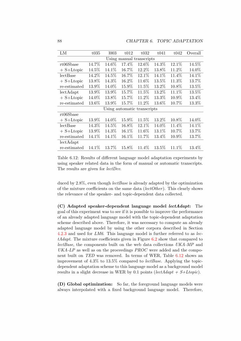
88 CHAPTER 6. TOPIC ADAPTATION
LM t035 l003 t012 t032 t041 t042 OverallUsing manual transcripts
rt06Sbase 14.7% 14.6% 17.4% 12.6% 14.3% 12.1% 14.5%+ S+Ltopic 14.5% 14.1% 16.7% 12.2% 13.8% 11.2% 14.0%lectBase 14.2% 14.5% 16.7% 12.1% 14.1% 11.4% 14.1%+ S+Ltopic 13.8% 14.3% 16.2% 11.6% 13.5% 11.3% 13.7%re-estimated 13.9% 14.0% 15.9% 11.5% 13.2% 10.8% 13.5%lectAdapt 13.9% 13.9% 15.7% 11.5% 13.2% 11.1% 13.5%+ S+Ltopic 14.0% 13.8% 15.7% 11.2% 13.3% 10.9% 13.4%re-estimated 13.6% 13.9% 15.7% 11.2% 13.6% 10.7% 13.3%
Using automatic transcriptsrt06Sbase+ S+Ltopic 13.9% 14.0% 15.9% 11.5% 13.2% 10.8% 14.0%lectBase 14.3% 14.5% 16.8% 12.1% 14.0% 11.4% 14.1%+ S+Ltopic 13.9% 14.3% 16.1% 11.6% 13.1% 10.7% 13.7%re-estimated 14.1% 14.1% 16.1% 11.7% 13.4% 10.9% 13.7%lectAdaptre-estimated 14.1% 13.7% 15.8% 11.4% 13.5% 11.1% 13.4%
Table 6.12: Results of different language model adaptation experiments byusing speaker related data in the form of manual or automatic transcripts.The results are given for lectDev.
duced by 2.8%, even though lectBase is already adapted by the optimizationof the mixture coefficients on the same data (lectOther). This clearly showsthe relevance of the speaker- and topic-dependent data collected.
(C) Adapted speaker-dependent language model lectAdapt: Thegoal of this experiment was to see if it is possible to improve the performanceof an already adapted language model with the topic-dependent adaptationscheme described above. Therefore, it was necessary to compute an alreadyadapted language model by using the other corpora described in Section4.2.3 and used for LM6. This language model is further referred to as lec-tAdapt. The mixture coefficients given in Figure 6.2 show that compared tolectBase, the components built on the web data collections UKA-MP andUKA-LP as well as on the proceedings PROC were added and the compo-nent built on TED was removed. In terms of WER, Table 6.12 shows animprovement of 4.3% to 13.5% compared to lectBase. Applying the topic-dependent adaptation scheme to this language model as a background modelresults in a slight decrease in WER by 0.1 points (lectAdapt + S+Ltopic).
(D) Global optimization: So far, the foreground language models werealways interpolated with a fixed background language model. Therefore,
6.3. LANGUAGE MODEL ADAPTATION EXPERIMENTS 89
it was analyzed if the WER improves when the mixture coefficients of thebackground language model were adjusted on the lectOther data as well.The mixture weights of the background language model and the foregroundlanguage models Stopic and Ltopic were optimized separately for each topicgroup. As can be seen in the rows of Table 6.12 labeled with re-estimated,the WER improved by 0.2 for lectBase and by 0.1 for lectAdapt. While forlectBase the WER for almost all talks and lectures was improved, for lec-tAdapt WER increases for l003 and t041. Especially for t041, the mixturecoefficients (which were averaged and optimized on t039 and t040) show ahuge difference compared to the coefficients optimized on t041 itself. In par-ticular, the Ltopic component should have had a coefficient of 0.21 insteadof 0.05.
Conclusion
Overall, the proposed topic dependent adaptation scheme, described at thebeginning of this section, can be used to adapt an unadapted language model(lectBase, WER 14.1%), such that an almost identical WER compared to ahighly adapted language model is achieved, i.e. 13.5% (re-estimated lectBasevs. lectAdapt). Furthermore, even an already adapted language model (lec-tAdapt), built using huge amounts of collected web data, was improved from13.5% to 13.3%. The best improvement was obtained, when the mixture co-efficients for all language model components were re-estimated instead ofusing the background language model as a single component.
6.3.6 Using Automatic Transcripts
The most interesting results were achieved when the automatically tran-scribed data was used instead of the manually transcribed data. The inter-polation weights for rt06Sbase were kept unchanged, but for lectBase andlectAdapt the mixture coefficients were re-estimated on ASR hypothesis oflectOther. As can be seen from the results given in Table 6.12, after S+Ltopicis applied to the background language models, the WER improved, but notby as much as when manually transcribed data is used. The differenceamounts to 0.2 for the re-estimated S+Ltopic lectBase LM, and to 0.1 iflectAdapt is used as a background LM.
Conclusion
The results in this Section show that automatic transcriptions from recordedtalks and lectures from past uses of the lecture translation system can beeasily used for adaptation. At an automatic transcription word error rateof less than 15%, a time consuming manual transcription of the recordingsis no longer necessary.

90 CHAPTER 6. TOPIC ADAPTATION
6.4 Expanding the VocabularyFor an efficient decoding process in a speech recognizer, a fixed vocabularyis indispensable, because only then can the search network be precomputedand optimized for decoding speed. In addition, an increase in the vocab-ulary size always involves an increase in decoding speed due to the largersearch space, as well as in an increase in memory requirements due to theincreased number of transitions in the n-gram language model. On the otherhand, with a fixed vocabulary, out-of-vocabulary (OOV) words cannot berecognized, and each occurrence of an OOV word is in average responsiblefor 1.5–2 recognition errors [GFS98].
Generally, the recognizer’s vocabulary is selected in order to obtain anOOV-Rate which is as low as possible on the target task or domain by mini-mizing the OOV-Rate on a related development set [IO99, VW03]. Technicaltalks and lectures have a narrow vocabulary, but the vocabulary can differlargely from talk to talk due to the technical terms and expressions. Inaddition, correct recognition of especially these technical terms and expres-sions is very important for the understanding of the context of the talk. Thesame is true for proper names which are often missing in the recognizer’svocabulary.
As in [RS02], a method was developed to decrease the OOV-Ratebased on presentation slides and on the Sseed corpus. In order to preventmisspellings, the selection of words per topic has to be performed semi-automatically. The developed heuristic is based on the assumption that thelonger the word, the more meaningful and relevant it is:
1. Select all non-singleton words from a given corpus which do not existin the baseline vocabulary.
2. Remove all words shorter than three characters.
3. Check all words from four up to six characters manually, and removeall meaningless words.
4. All words left will be used for vocabulary adaptation.
In order to use the additional words in the speech recognizer, pronun-ciations have to be generated. Therefore, the pronunciation generator de-veloped for the RT-06S evaluation [FIK+06] was used, which first tries tofind the word in a large background pronunciation dictionary, and, if notfound, uses the Festival [BT97] speech synthesis system for pronunciationgeneration.
We pose the question of how to add the selected words to the languagemodel. If the frequency of the words in the given corpus is low, usingthis corpus as is for language modeling might underestimate their transitionprobabilities. While for the large Stopic corpus this might not be a problem,

6.4. EXPANDING THE VOCABULARY 91
talk OOV WER OOV WER OOV WER OOV WERbaseline general specific both
t035 0.62 13.9% 0.32 13.5% 0.34 13.6% 0.30 13.6%l003 0.45 14.0% 0.28 13.6% 0.25 13.7% 0.22 13.6%t012 0.45 15.9% 0.27 16.0% 0.45 15.8% 0.27 15.8%t032 0.37 11.5% 0.30 11.3% 0.37 11.2% 0.30 11.2%t041 1.08 13.2% 0.97 13.0% 0.97 12.9% 0.92 12.9%t042 0.62 10.8% 0.44 10.9% 0.62 10.9% 0.44 10.9%Overall 0.49 13.5% 0.33 13.3% 0.38 13.2% 0.30 13.2%lectAdapt 13.0%
Table 6.13: Comparison of OOV-Rates and WERs for different expansionsof the vocabulary on lectDev. As baseline language model, the re-estimatedS+Ltopic lectBase language model was used for the detailed results. Theresult in the last row was achieved with a similar adapted lectAdapt LM.WERs were obtained after performing language model rescoring.
using the presentation slides for language modeling might not be a goodidea. Furthermore, it cannot be guaranteed that the selected words occurfrequently enough in the collected Ltopic corpus. Therefore, all selectedwords were added to a special class in the language model, i.e. the unknownword class, to which all words not in the vocabulary are mapped duringlanguage modeling. The unigram probability of the unknown word classfor large corpora is typically comparable to the probability of ’a’, which israther high. An uniform distribution is used as the intra-class distributionfor the selected words, because the frequency of the selected words in thecorpus does not match real usage.
As shown by Schaaf [Sch04] by adding the new words to a single unknownword class as described above, relatively good recognition accuracy could beachieved. However, when adding a large number of words, this method maybe disadvantageous because the words are indistinguishable from a languagemodel point of view. Schaaf investigated also more sophisticated methodsin which several unknown word classes were incorporated in the languagemodel. Words are then added to one or multiple classes. Therefore, theexperiments described in the following should be seen as a first prove of theabove described selection procedure. It can be expected that improvementsobserved by adding the selected words to a single unknown word class carryover when multiple classes are used.
6.4.1 Experiments
Table 6.13 shows the WERs together with the OOV-Rates achieved withdifferent expansions of the vocabulary. The re-estimated S+Ltopic lectBase

92 CHAPTER 6. TOPIC ADAPTATION
language model was used as the baseline language model for the results inthe top part of the table. As can be seen, the baseline vocabulary achievedan overall OOV-Rate of 0.49 and an overall WER of 13.5%. In the followingthree experiments it will be shown that the selected words improve therecognition results. In the first experiment, words were selected from theStopic corpus and in the second experiment from the presentation slides. Inthe last experiment both selections were combined.
Extracting words from general speaker related data
The above described heuristic selected 715 words from the Stopic corpus.As can be seen in the columns labeled as general in Table 6.13, the overallOOV-Rate was reduced by 33% to 0.33 and the overall WER to 13.3%.From the detailed results, it can be seen that not all talks or lectures benefitfrom the selected words. For t012 and t044 the WER increases slightlyalthough the OOV-Rate decreased significantly. The reason for this is theabove described problem when adding too many words to a single class usingan uniform intra-class probability distribution.
Extracting words from the presentation slides
In this experiment, the heuristic was used to select words from the presen-tation slides. The number of words selected, ranged from 2 to 182, with anaverage of 40. Although the OOV-Rate is higher than compared to the firstexperiment, the overall WER could be reduced to 13.2% (column labeled asspecific in Table 6.13). The reasons for this difference to the first experimentare that first, the amount of words selected is smaller and therefore betterdistinguishable, and, second, the words selected are more relevant.
The combination of both selections
In the last experiment, both selections were combined. As can be seen fromthe results in the column labeled as both in Table 6.13 the overall OOV-Ratewas further reduced to 0.30 but the overall WER remained constant.
Conclusion
Overall, the developed vocabulary selection heuristic was able to reduce theOOV-Rate by 39% and the WER by 2.2% relative. But, as already ex-pected, adding all selected words to a single class is unsuitably when thenumber of words selected is large. If the re-estimated S+Ltopic lectAdaptlanguage model was used instead of the re-estimated S+Ltopic lectBase lan-guage model, the overall WER was reduced by 2.3% relative to 13.0%.

6.5. TOPIC ADAPTATION FOR MACHINE TRANSLATION 93
6.4.2 Handling of foreign words
If a speech recognizer is developed for a single language, the phoneme set typ-ically covers pronunciations restricted to that language only. This makes itdifficult to model foreign words coming from other languages such as propernames, because the necessary phonemes do not exist in the recognizer. Asan example, it is difficult to model German umlauts such as in the thesisauthor’s last name “Fügen” with an English recognizer. For the recognitionof technical talks or lectures in other languages, this is even more a problembecause many technical terms exist in English only due to the dominanceof English for international communication. Moreover, the pronunciation of“Fügen” depends on the mother tongue of the speaker and on the speaker’sexperience with foreign languages. An English native speaker might pro-nounce “Fügen” differently from a German native speaker giving a talk inEnglish.
The key to a solution is the use of a multilingual acoustic model [SK06]instead of a monolingual one. This makes it possible to model foreign wordsin other languages with the corresponding phoneme sequence. Moreover,further pronunciation variants can be added with phonemes of other lan-guages to support non-native pronunciations of the same word. A disadvan-tage is that the recognizer increases in size and complexity. Furthermore,depending on the modeling technique, the introduced pronunciation variantsmay cause the recognition accuracy to suffer. Modeling techniques can rangefrom completely language-independent acoustic models, over cross-languageacoustic models [SW01], up to cross-language acoustic and language models[FSS+03, HHP01]. With the latter technique, it is possible to use the samerecognizer for two or more languages.
For the developed prototype of a simultaneous translation system, mul-tilingual acoustic models were not used because the expected performancegain was small on the given data set.
6.5 Topic Adaptation for Machine Translation
Adaptation of the MT component of the baseline translation system towardsthe more conversational style of lectures and known topics was accomplishedby a higher weighting of the available lecture data in two different ways.First, for computing the translation models, the small lecture corpora wereduplicated several times and added to the original EPPS training data. Thisyielded a small increase in MT scores (see Figure 6.15).
Second, for (target) language model adaptation, web data was collected.As can be seen in Table 6.14, the baseline EPPS-T language model basedon EPPS text data only has a very high perplexity. Therefore, two differentweb data collections were performed. For further adaptation of the languagemodel to the more conversational style of lectures, common spontaneous
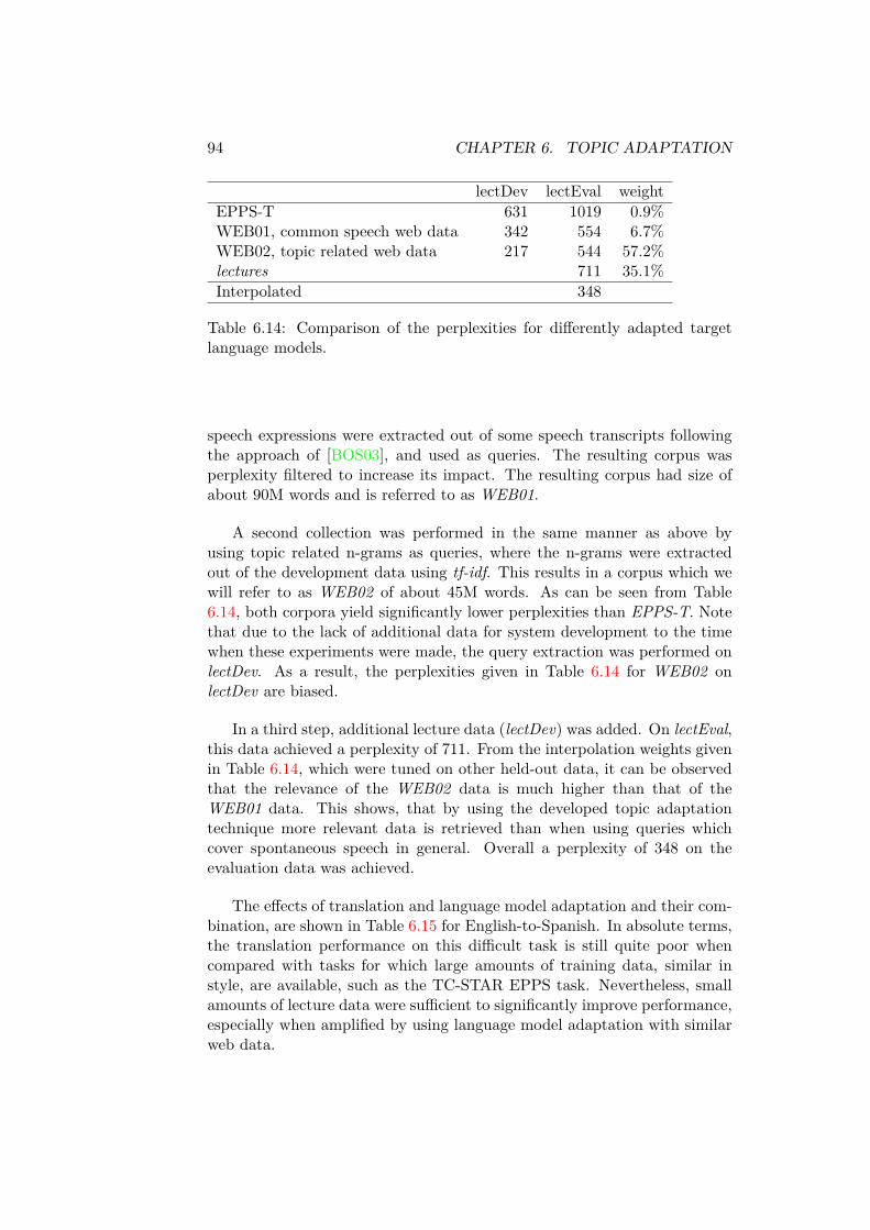
94 CHAPTER 6. TOPIC ADAPTATION
lectDev lectEval weightEPPS-T 631 1019 0.9%WEB01, common speech web data 342 554 6.7%WEB02, topic related web data 217 544 57.2%lectures 711 35.1%Interpolated 348
Table 6.14: Comparison of the perplexities for differently adapted targetlanguage models.
speech expressions were extracted out of some speech transcripts followingthe approach of [BOS03], and used as queries. The resulting corpus wasperplexity filtered to increase its impact. The resulting corpus had size ofabout 90M words and is referred to as WEB01.
A second collection was performed in the same manner as above byusing topic related n-grams as queries, where the n-grams were extractedout of the development data using tf-idf. This results in a corpus which wewill refer to as WEB02 of about 45M words. As can be seen from Table6.14, both corpora yield significantly lower perplexities than EPPS-T. Notethat due to the lack of additional data for system development to the timewhen these experiments were made, the query extraction was performed onlectDev. As a result, the perplexities given in Table 6.14 for WEB02 onlectDev are biased.
In a third step, additional lecture data (lectDev) was added. On lectEval,this data achieved a perplexity of 711. From the interpolation weights givenin Table 6.14, which were tuned on other held-out data, it can be observedthat the relevance of the WEB02 data is much higher than that of theWEB01 data. This shows, that by using the developed topic adaptationtechnique more relevant data is retrieved than when using queries whichcover spontaneous speech in general. Overall a perplexity of 348 on theevaluation data was achieved.
The effects of translation and language model adaptation and their com-bination, are shown in Table 6.15 for English-to-Spanish. In absolute terms,the translation performance on this difficult task is still quite poor whencompared with tasks for which large amounts of training data, similar instyle, are available, such as the TC-STAR EPPS task. Nevertheless, smallamounts of lecture data were sufficient to significantly improve performance,especially when amplified by using language model adaptation with similarweb data.

6.6. CONCLUSION 95
Unadapted TM-adapt +LM-adaptNIST BLEU NIST BLEU NIST BLEU
t036+, text input 5.72 23.4 5.89 25.0 6.33 28.4t036+, ASR input 5.06 17.9 5.15 18.9 5.60 23.0l043, text input 5.27 19.6 5.35 20.3 5.48 21.6l043, ASR input 4.80 16.6 4.85 16.9 5.05 19.0
Table 6.15: Translation model and language model adaptation. t036+ is amerge of t036 and t037.
6.6 Conclusion
In this chapter, an adaptation framework for lectures and speeches was pro-posed. Depending on the amount of information available for a particularspeaker or topic, different adaptation levels can be used within a simulta-neous translation system. While the previous chapter’s focus was acousticmodel-based speaker adaptation, this chapter’s main focus was topic adapta-tion. The proposed technique is the collection of additional speaker-relatedor on-topic data which is used for linear interpolation with a backgroundlanguage model. The data is collected through the Internet by querying asearch engine and retrieving and filtering the resulting web pages. For queryextraction, a tf-idf -based heuristic was developed, which computes tf-idfweights for n-grams instead of single words and uses these weights togetherwith frequency-based thresholds. The n-grams were extracted from a seedcorpus, i.e. either manually collected speaker information such as researchpapers (Sseed) or presentation slides (Lseed), and each of the extracted n-grams was used as a single query. The main problem is the optimizationof the mixture coefficients for the mixture language model. The better thedata match in speaking style and topic, the better can the resulting mix-ture language model be expected to perform. Therefore, several differentdata sets were tested for suitability, from data matching in speaking style todata matching also in topic. Adaptation by using the reference transcriptsand adaptation by using the speech recognizer’s hypotheses was compared.Significant improvements were observed on RT-06SDev as well as on lectDev.
Using speaker-related information only, three-fold language model inter-polation improved the word error rate by 3.8% on lectEval. For interpolation,language models built from the seed corpus (Sseed), the corpus collectedfrom n-grams extracted from the seed corpus (Stopic), and an unadaptedbackground language model (rt06Sbase) was used. The mixture coefficientswere optimized globally on some held-out data.
When other talks or lectures of the speaker were available, this data(lectOther) was used for further language model adaptation. First, the un-adapted background language model was optimized on lectOther, leading
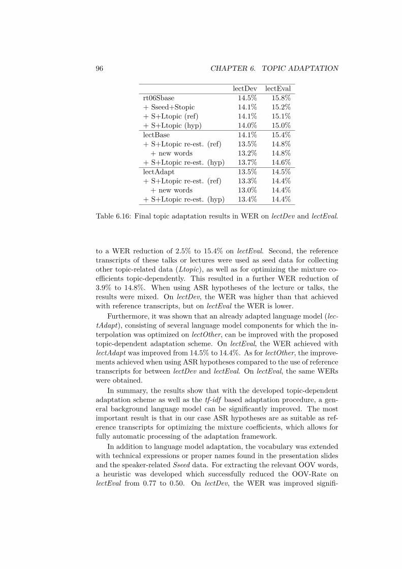
96 CHAPTER 6. TOPIC ADAPTATION
lectDev lectEvalrt06Sbase 14.5% 15.8%+ Sseed+Stopic 14.1% 15.2%+ S+Ltopic (ref) 14.1% 15.1%+ S+Ltopic (hyp) 14.0% 15.0%lectBase 14.1% 15.4%+ S+Ltopic re-est. (ref) 13.5% 14.8%+ new words 13.2% 14.8%
+ S+Ltopic re-est. (hyp) 13.7% 14.6%lectAdapt 13.5% 14.5%+ S+Ltopic re-est. (ref) 13.3% 14.4%+ new words 13.0% 14.4%
+ S+Ltopic re-est. (hyp) 13.4% 14.4%
Table 6.16: Final topic adaptation results in WER on lectDev and lectEval.
to a WER reduction of 2.5% to 15.4% on lectEval. Second, the referencetranscripts of these talks or lectures were used as seed data for collectingother topic-related data (Ltopic), as well as for optimizing the mixture co-efficients topic-dependently. This resulted in a further WER reduction of3.9% to 14.8%. When using ASR hypotheses of the lecture or talks, theresults were mixed. On lectDev, the WER was higher than that achievedwith reference transcripts, but on lectEval the WER is lower.
Furthermore, it was shown that an already adapted language model (lec-tAdapt), consisting of several language model components for which the in-terpolation was optimized on lectOther, can be improved with the proposedtopic-dependent adaptation scheme. On lectEval, the WER achieved withlectAdapt was improved from 14.5% to 14.4%. As for lectOther, the improve-ments achieved when using ASR hypotheses compared to the use of referencetranscripts for between lectDev and lectEval. On lectEval, the same WERswere obtained.
In summary, the results show that with the developed topic-dependentadaptation scheme as well as the tf-idf based adaptation procedure, a gen-eral background language model can be significantly improved. The mostimportant result is that in our case ASR hypotheses are as suitable as ref-erence transcripts for optimizing the mixture coefficients, which allows forfully automatic processing of the adaptation framework.
In addition to language model adaptation, the vocabulary was extendedwith technical expressions or proper names found in the presentation slidesand the speaker-related Sseed data. For extracting the relevant OOV words,a heuristic was developed which successfully reduced the OOV-Rate onlectEval from 0.77 to 0.50. On lectDev, the WER was improved signifi-

6.6. CONCLUSION 97
cantly, but on lectEval no improvement was observed. An explanation forthis may be the use of a single class in the language model to which all newwords are added. More classes, as proposed in [Sch04, RS02], may need tobe used.
The tf-idf -based query generation and web-data collection technique wasalso successfully used for target language model adaptation in the machinetranslation component. With four-fold interpolation consisting of the Euro-pean Parliament Plenary Session-based background language model, someSpanish lectures from lectDev and two language models build from web data,the perplexity on lectEval was reduced from 1019 to 348. One web corpuswas collected with common spontaneous speech expressions, the other oneby using the proposed tf-idf -based topic collection technique. As a result ofthe perplexity reduction, the translation quality on ASR hypotheses of a sys-tem in which the translation model is already adapted was further improvedsignificantly by 21.7% to 23.0% for t036+ and 12.4% for l043.

98 CHAPTER 6. TOPIC ADAPTATION

Chapter 7
Latency and Real-Time
As already described in the introductory chapters, simultaneous interpreta-tion is in contrast to consecutive interpretation defined by an interpretationof the source speech as quickly as possible. Hereby, the length of the ear-voice-span or latency depends on the grammatical structure of the sourceand target language, but should be as short as possible. Therefore, thewhole system requires high processing speed of the components and a shortlatency. On the other hand, a good recognition and translation quality isrequired to facilitate a fluent translation. But speed and quality are two sys-tem attributes, which are orthogonal to each other — increasing the speedof a system often reduces its quality and vice versa.
This chapter deals with the question on how and to what extent thespeed and latency of the system can be increased without loosing to muchrecognition and translation quality. To increase the processing speed, tun-ing can be done with respect to single components; however, shortening thelatency requires adjustments to the whole framework. To shorten the la-tency, it is necessary to de-serialize the processing, in which the ASR startsto decode when the recording is finished and transmits the hypothesis to theMT not until the decoding has been finished, to an overlapped processing.Further speed-up can be achieved if the ASR component transmits partialhypothesis while decoding the current recording as shown in Figure 7.1.This allows the MT component to start earlier.
To support this kind of processing, incremental adaptation and the lan-guage model have to be adjusted in the ASR component; the Ibis decoderused in this thesis already processes the data time-synchronously, i.e. frame-by-frame. On the other hand, the non-linearity of the translation process,due to possible re-orderings of words or phrases makes the same changes inthe MT component much more complicated. Therefore, almost all currentmachine translation systems require sentence-like units as input which arethen translated as a whole. For this reason a Resegmentation componentwas introduced, which is responsible for chunking the continuous output
99

100 CHAPTER 7. LATENCY AND REAL-TIME
MT
ASR
Recording
MT
Resegmentation
ASR
Recording
t
Serial
Overlapping
Figure 7.1: Comparison of serial and overlapping processing.
stream of the speech recognizer into smaller segments for which the trans-lation quality does not suffer.
The remainder of this chapter focuses on the real-time and latency as-pects of a simultaneous translation system. The Resegmentation componentwill be discussed in Chapter 8. To increase the real-time of a speech recog-nizer, search-space pruning and Gaussian selection techniques are analyzedin Section 7.2 and 7.3 using the Ibis decoder. In Section 7.4, methods areintroduced to reduce the latency of the serialization, and their influence onincremental adaptation and recognition quality are analyzed. Section 7.5concludes this chapter.
For the following experiments, several different acoustic models weretrained on the same training data as used for the baseline system, whichwas described in Section 4.2.1. They differ by the overall number of code-books (m ∈ 3000, 4000, 6000) and the maximum number of Gaussians percodebook (n ∈ 64, 128, 256) and are named with m−n for an acoustic modelwith m codebooks and a maximum number of n Gaussians per codebook.If not otherwise specified, all acoustic models were trained up to step 5 ofthe training procedure described in Section 4.2.1. Acoustic model speci-fiers tagged with MMIE are trained up to step 9. The acoustic model usedfor the baseline system described in Section 4.3.7 is referred to as 4000-64-mmie. Table 7.1 shows the total number of Gaussians available in each ofthe acoustic models together with its word error rate and real-time factor.If not otherwise stated, the real-time factor of the decoding process itself isgiven, without the time necessary for incremental adapting the cMLLR andVTLN parameters, and is referred to as RTF or RTF decoding. RTF totalrefers to the total amount including adaptation.

7.1. SPEED-UP TECHNIQUES FOR SPEECH RECOGNITION 101
acoustic model number of Gaussians WER RTF3000-64 184254 15.6% 1.343000-128 328623 15.3% 1.713000-256 497728 14.9% 2.184000-64 232046 15.5% 1.254000-128 390774 15.1% 1.774000-256 539345 14.9% 2.136000-64 316917 15.4% 1.34
Table 7.1: Overview of the total umber of Gaussians for each acoustic modeltogether with its word error rate on lectDev.
Search Layer
Input Layer
Execution Layer
Grammar LayerGaussian Layer
Layer ExamplesInput Layer Frame-skipping, down-samplingSearch Layer Beam search, search-space pruningGaussian Layer Gaussian selectionGrammar Layer Language model lookaheadExecution Layer SIMD, compiler optimizations
Figure 7.2: A five layer model for the categorization of optimization strate-gies of a speech recognizer.
7.1 Speed-up Techniques for Speech Recognition
Following [Kö04, CSMR04], a five-layer model for the categorization of opti-mization strategies of a speech recognizer is introduced and shown in Figure7.2. The motivation behind this model is that single optimizations can becategorized into one level and that optimizations on different levels havemore likely a greater impact in reducing the decoding speed, than comparedto different optimizations on the same level, because they are independentto each other. In contrast to [Kö04, CSMR04] the presented model cate-gorizes the whole decoder into 5 different layers instead of categorizing theGaussian mixture model computation only.
The Execution Layer covers all techniques related to the execution ofthe decoding process. This includes manual optimizations such as the use

102 CHAPTER 7. LATENCY AND REAL-TIME
of SIMD (single input, multiple data) instructions for matrix operationsand observation probability estimation [KSN00], as well as automatic op-timizations made by modern compilers. In this thesis, for compiling Ibis,the following settings were used in combination with Intel’s C++ Compiler10.1 for Linux on a 64bit CPU: -axW -O3 -ip -parallel. This gener-ates specialized code paths for SSE2 and SSE instructions for Intel proces-sors (-axW), turns on aggressive optimizations such as loop and memoryaccess transformation, turns on pre-fetching (-O3), enables additional intra-file inter-procedural optimizations (-ip), and uses the auto-parallelizer togenerate multi-threaded code for loops that can be safely executed in par-allel (-parallel) [Int08]. Compared to no optimization at all, the result-ing speed-up can range from 10%-20%. In another experiment, a manualoptimization of the observation probability computation by using SIMD in-structions similar to [KSN00] was compared to the automatic optimizationsof the Intel compiler, and no difference in performance could be measuredbetween the two.
Techniques belonging to the Input Layer are responsible for reducingredundancies in the input stream, i.e. the sequence of observation vectors.Well-known techniques are the so-called frame-skipping or down-sampling.While down-sampling [CSMR04] reduces the amount of data in the inputstream by just taking every n-th observation vector, frame-skipping is moreintelligent. Only those observation vectors are ignored for which the distanceto the preceding vector is smaller than a given threshold [Wos98, KFSW05].Another common approach is to use a voice-activity detector to removeobservation vectors which can be classified as non-speech.
In the Search Layer, all techniques are concentrated which focus on op-timizing the decoding process itself as well as the architecture used for rep-resenting the search space. Search-space pruning is one technique whichcan be categorized in this layer, architectural optimizations such as pro-nunciation prefix trees together with the linguistic polymorphism used inIbis also belongs to it. Both will be explained below. Other architecturesuse weighted finite-state transducers (WFST), which allow to efficiently en-code all the various knowledge sources. The network resulting from thecomposition of these WFSTs, after minimization, can be directly used in aViterbi decoder [MPR00, SPZ05]; this approach has been shown to be quitepromising [KNRM02].
Closely related to the Search Layer are optimizations categorized in theGaussian and Grammar Layer. Two widely used techniques for speedingup the observation probability computation in the Gaussian Layer, the BBIalgorithm and Gaussian Clustering, will be discussed below. For fast accessto the language model probabilities, the use of a language model lookaheadtree is very common [ONE96]. Pruning and smoothing techniques are alsoused for language models, but are more related to reducing the size of thelanguage models instead of accelerating the probability computation. In

7.2. SEARCH-SPACE PRUNING IN IBIS 103
R D
W EY
AH
LB
OA
T
IE
lct= "a new"
lct= "little late"
lct= "much more"
lct= "bullets over"
B
lct= "bullets over"
lct= "a new"
R
AH
lct= "bullets over"
lct= "a new"
lct= "little late"
lct= "much more"
EY
IE
lct= "much more"
Figure 7.3: A simple pronunciation prefix tree without and with linguisticmorphed instances for a system using context independent acoustic models.“lct” stands for linguistic context.
fact, for the commonly used n-gram back-off language models, pruning canslow down the probability computation, because the backing-off to lowern-grams needs additional memory accesses.
Independent of algorithmic improvements are the quality of the acousticand language models. The effectiveness of several of the above mentionedtechniques depends on the similarity between training and testing condi-tions.
7.2 Search-Space Pruning in Ibis
The search-space of the decoder is restricted by the number of pronuncia-tions in the dictionary and the size of the acoustic model. An elegant wayof representing the search-space of a speech decoder is by using pronunci-ation prefix trees (PPTs). A pronunciation prefix tree is generated out ofthe pronunciation dictionary by merging identical phone sequences of dif-ferent dictionary entries and convolving them with the acoustic model. Asimple example for context independent acoustic models is given in Figure7.3. For further compactification of the search-space, Ibis allows compress-ing the PPT into a search network by removing other redundancies betweendifferent branches with an iterative algorithm.
When reaching the end of a PPT, i.e. its leafs, it becomes necessary toextend the search to the following word candidates. This can be done eitherby creating a copy of the tree or by re-entering the tree and keeping trackof the word history. The idea of the tree copy process [NHUTO92, Ode95,OEN98, Aub99] is to create a separate copy for each surviving linguistic

104 CHAPTER 7. LATENCY AND REAL-TIME
state1 after path recombination. Since the number of different linguisticstates, i.e. tree copies, can be a few hundred for a long-span languagemodel, efficient pruning is necessary. Ibis uses an alternative approach tothe tree copying process, which is based on a single PPT. Therefore, alinguistic polymorphism as described in [SMFW01, SMFW02] and similarto [AHH96, FKFW99] was introduced. In each node of the PPT, a list oflinguistically morphed instances is kept, and each instance stores it’s ownback-pointer and score for the underlying Hidden Markov Model (HMM)with respect to the linguistic state of this instance. Since the linguisticstate is known, the complete language model information can be applied ineach node of a PPT. The advantage of this search-space organization is thatefficient pruning can be applied, which eliminates the sub-tree dominanceproblem of the tree copy approach.
Pruning within the search network can now be performed at differentlevels and by using different techniques. To clarify the experiments in thefollowing sections, the levels will be described shortly. In the description,the values in parenthesis are the default pruning parameters. Ibis is a time-synchronous decoder, which means that in each frame all active decodingpaths are expanded and pruned before entering the next frame, and all activedecoding paths end at the current frame. A decoding path is active, if itwill be expanded in the next frame, i.e. was not not pruned. Pruning canbe either done relative to the current best, or by taking the top N best outof a sorted set of paths.
State Level: All states of the underlying HMM structure belong to thestate level. Pruning at the state level means that transitions from onestate to another state are done only, if the transition score is not ex-ceeding a specific threshold. This threshold is defined relative to thescore of the best state transition in the current frame. Pruning is per-formed after all transition scores for the current frame are computed.(stateBeam=130)
Linguistic Instance Level: All linguistic morphed instances, i.e. allpaths which are in the same HMM state for the current frame, but havedifferent linguistic contexts, belong to the linguistic instance level. Allinstances with the same HMM state are combined in a single PPTnode. Especially, if the path comes to an word-end, i.e. PPT leaf, it isimportant to keep the numbers of instances per state as small as pos-sible to reduce the computational effort due to the fan-out of the rightcontext models for starting the new words. Therefore, new instanceswill not be added if their score exceeds a threshold relative to the bestscore in a PPT node. Furthermore, the numbers of instances per node
1The current word represented by the PPT leaf and it’s predecessor words are referredto as the linguistic state.

7.2. SEARCH-SPACE PRUNING IN IBIS 105
are pruned to a fixed number using topN pruning. (morphBeam=80,morphN=10)
Word Level: Transitions from the last state of one word to the next state ofanother word, is not allowed, if the score exceeds a threshold relative tothe best score of the current frame. Furthermore, the number of thesetransitions is reduced with the help of a topN pruning. In contrastto the pruning at the linguistic instance level, which is done per nodeonly, the pruning at the word level limits the overall number of wordswhich can be followed in the next frame. (wordBeam=90, transN=40)
A so called master beam (default mb=1.0) can be used to adjust allrelative pruning parameters by a given factor.
7.2.1 Experiments and Discussion
The goal of the following experiments is to show the relationship of differentpruning and language model parameters and their influence on decodingspeed and error rate. Since the Ibis decoder is a single-pass decoder, anothergoal was to evaluate the possible improvement due to a second languagemodel rescoring pass. As a baseline, the decoding performance using defaultpruning (see above) and language model parameters was used. Specifically,a language model weight of 26 and a word penalty of 6 without any languagemodel rescoring was used.
First, the relationship of all relative pruning parameters was analyzed.All language model and topN pruning parameters were kept at the defaultvalues. From Figure 7.4, it can be observed that the state beam has thelargest influence on recognition accuracy. Changes in the word beam onlyslightly influence WER down to a value of around 70-80, but values belowthis break-point result in a rapid increase of WER. The same is true for themorph beam, where the break-point is around 50-60. In terms of decodingspeed, it can be seen that there is a almost linear correlation between allrelative pruning parameters and the real-time factor, besides morph beam,which does not influence the real-time factor at values larger than 50.
Figure 7.5 concentrates on the relationship between all topN pruningparameters with respect to the WER and RTF. All language model and rel-ative pruning parameters were kept fixed. Regarding transN, it can be seenthat there is almost no change in WER down to a value of 12. Below thisbreak-point WER begins to increase. For morphN, the break-point in WERis at 3. Decoding speed increases continuously with decreasing transN andmorphN, and the influence is larger for transN than for morphN especiallyfor small transN. This is clear because the smaller the allowed number oftransitions, the smaller the number of possible linguistically morphed in-stances. Given these results, by tuning the topN pruning parameters the

106 CHAPTER 7. LATENCY AND REAL-TIME
baselinestate beam=120state beam=130state beam=140state beam=150
10 30
50 70
90 110word beam 0
20 40
60 80
100 120
morph beam
16
18
20
22
24
WER [%]
baselinestate beam=120state beam=130state beam=140state beam=150
10 30
50 70
90 110word beam 0
20 40
60 80
100 120
morph beam
0
0.5
1
1.5
2
RTF
Figure 7.4: The relationship of different relative pruning parameter settingsto word error rate (WER) and decoding speed (RTF) in Ibis. For the base-line, decoding was done with default pruning and language model parametersettings.
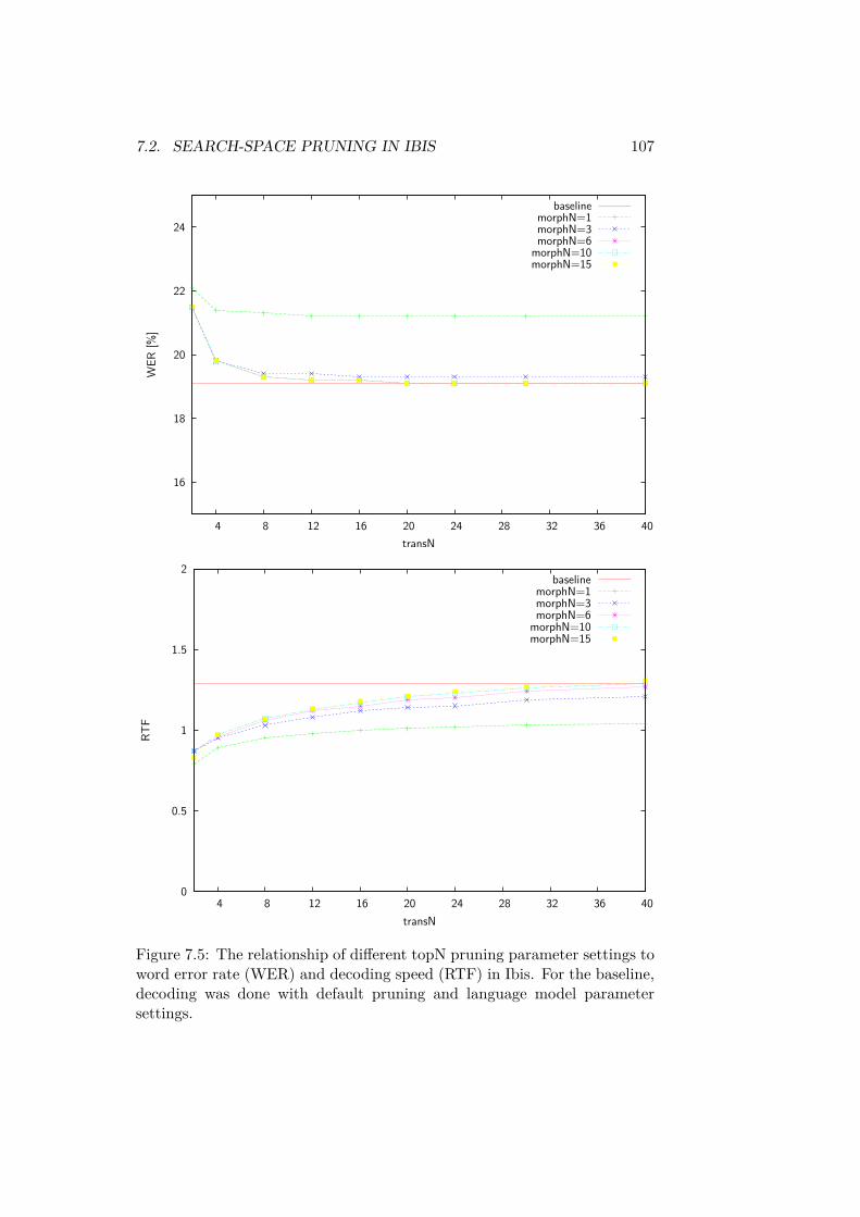
7.2. SEARCH-SPACE PRUNING IN IBIS 107
16
18
20
22
24
4 8 12 16 20 24 28 32 36 40
WER
[%]
transN
baselinemorphN=1morphN=3morphN=6
morphN=10morphN=15
0
0.5
1
1.5
2
4 8 12 16 20 24 28 32 36 40
RTF
transN
baselinemorphN=1morphN=3morphN=6
morphN=10morphN=15
Figure 7.5: The relationship of different topN pruning parameter settings toword error rate (WER) and decoding speed (RTF) in Ibis. For the baseline,decoding was done with default pruning and language model parametersettings.

108 CHAPTER 7. LATENCY AND REAL-TIME
WER RTFbaseline 4000-64-mmie 14.3% 1.07
4000-128-mmie 14.4% 1.573000-64-mmie 14.4% 1.163000-256-mmie 14.6% 2.01
optimized 4000-64-mmie 14.6% 0.894000-128-mmie 14.6% 1.223000-64-mmie 14.6% 0.883000-256-mmie 14.7% 1.51
Table 7.2: Comparison of recognition accuracy and decoding speed betweendifferent acoustic models using default or optimized pruning parameters fordecoding on lectDev. For the optimized results a state beam of 130, wordbeam of 80, morph beam of 60, transN of 20, and a morphN of 6 was used.
decoding speed can be increased without significant increase in WER. AtransN of 20 and a morphN of 6 seem to be optimal.
Altogether, with the improved pruning parameter settings, the real-timefactor could be improved by 17% to 0.89 for the baseline system (4000-64-mmie) with an increase in WER by 2.1% to 14.6%. The optimized pruningparameters also hold for systems using other acoustic model sizes, as can beseen in Table 7.2. The improvement for the 3000-64-mmie is even larger;the RTF is reduced by 24% while the WER increases by only 1.4%.
Language Model Rescoring
In a single pass decoder, all knowledge sources are typically integrated asearly as possible into the score computation. An example for this is the lan-guage model score, for which the exact score is applied as soon as the wordidentity is known. This can be already before a leaf node of the pronun-ciation prefix tree is reached. Prior to this, the best language model scoregiven all possible words through the current state is applied. The followingexperiments intend to show whether a language model rescoring using theword lattice produced during decoding can still improve performance, andif the same improvement with respect to WER and RTF is possible usingdifferent language model and pruning parameters already during decoding,i.e. without the necessity of a rescoring.
For speech recognition, we seek to find the sequence of words w that max-imizes the posterior probability for a given sequence of acoustic observation

7.2. SEARCH-SPACE PRUNING IN IBIS 109
vectors o
w = argmaxw
P (w|o)
= argmaxw
p(o|w) · P (w)p(o)
= argmaxw
p(o|w) · P (w)
where p(o|w) is modeled by the acoustic model and P (w) by the languagemodel. Due to different model spaces, the variances and means of the acous-tic and language model probabilities heavily deviate from each other. As aresult of this a language model weight has to be introduced. Additionally, aword penalty has to be introduced, which depends on the length of the cur-rent hypothesis to prefer the recognition of longer words over shorter ones[Rog97]. With these additional parameters and after transforming all prob-abilities into the log-domain, the score logP (w|o) is computed as follows
logP (w|o) = log(p(o|w) · P (w)lz · q|w|)= log p(o|w) + lz logP (w) + |w| log q= log p(o|w) + lz logP (w) + |w|lp
with |w| being the length of the word sequence w, lz the language modelweight, and lp the word penalty.
Given the explanations above, it follows that, given a fixed acoustic andlanguage model, changes in lz linearly scale the overall score, while changesin lp cause an additive shift of the scores depending on the length of thehypothesis. For single-pass decoding with Ibis, this means that to achievethe same WER after scaling lz and lp, further referred to as language modelparameters, all relative pruning parameters have to be scaled as well.
This is exactly the behavior which can be observed in the top plot of Fig-ure 7.6. The figure shows the correlation between different language modeland relative pruning parameters with respect to WER. All topN pruningparameters were kept unchanged. As expected, if the relative pruning pa-rameters were kept unchanged as well, the WER increases as lz increases.However, if the relative pruning parameters are increased as well, the WERimproves as lz increases. The influence of the word penalty on the overallrecognition accuracy is rather small.
On the other hand, the more the relative pruning parameters and lz areincreased, the less the considerations of variations in the acoustic model scoreduring pruning. As a result, more acoustic model scores will be computedand decoding is getting slower. The lower plot of Figure 7.6 confirms this. Iflz is increased without changing the relative pruning parameters, the real-time-factor decreases. If the relative pruning parameters are increased aswell, the real-time factor increases.

110 CHAPTER 7. LATENCY AND REAL-TIME
baselinerescoredmb=0.8mb=1.0mb=1.2mb=1.4mb=1.6
20 25
30 35
40 45language model weight (lz) 0
2 4
6 8
10 12
word penalty (lp)
10 15 20 25 30 35
WER [%]
baseline/ rescoredmb=0.8mb=1.0mb=1.2mb=1.4mb=1.6
20 25
30 35
40 45language model weight (lz) 0
2 4
6 8
10 12
word penalty (lp)
0 1 2 3 4 5
RTF
Figure 7.6: The relationship of different pruning and language model param-eters and their influence on error rate (WER) and decoding speed (RTF) inIbis. For the baseline, decoding was done with default pruning and languagemodel parameter settings.

7.3. GAUSSIAN SELECTION IN IBIS 111
When comparing both plots, it can be seen that although the same WERcan be achieved with other values of the relative pruning and language modelparameters, all settings with increased parameters result in an increase inRTF. Therefore, a two pass approach seems to be advantageous, in whichfirst, smaller language model parameters are used for the decoding, so thatthe acoustic model dominates the search process, and second, based on alattice a rescoring is performed with higher language model parameters inthis reduced search space. As can be seen from the results presented inthe figures, after language model rescoring the WER is decreased by 1%absolute with an immeasurable increase in RTF only.
7.3 Gaussian Selection in IbisFrom the experimental results in the section above, we have seen that thereis a break point in the pruning parameter space from which the relation-ship between decoding speed and accuracy drastically degrades, i.e. anyadditional increase in decoding speed results in a disproportional increase inWER. Therefore, to further increase the decoding speed other techniques,which can be used in addition to search-space pruning are necessary.
As already described in Section 4.3.4, in our case the baseline acousticmodel consists of about 4000 context dependent codebooks, each modeledwith a maximum of 64 Gaussians over a 42-dimensional feature space. Fora given input vector o and a single allophone2 modeled by an n-dimensionalGaussian mixture model, the scoring function for computing the observationprobabilities is defined as follows:
f(o = o1, . . . , on) =∑k
ωk1
(2π)n/2|Σk|1/2e−
12 (o−µk)TΣ−1
K (o−µk)
given that the Gaussian mixture model is represented with k componentsand each component with mean µk, a covariance matrix Σk, and mixturecoefficients ωk. For the baseline acoustic model, this means that k ≤ 64 andn = 42. Due to precision problems when multiplying a huge amount of verysmall values, the observation probability computation has to be done in thelog-domain and as a first speed-up only diagonal covariances are commonlyused, which results in the following equation:
log f(o = o1, . . . , on) = log∑k
elogωk− 1
2
(log((2π)n)+log(|Σk|)+
∑n
i=1(oi−µki)
2
σki
)Since the sum over all components is computationally very expensive, com-monly only the component for which the Mahalanobis distance to the cur-rent input vector o is the smallest is evaluated as an approximation (Nearest
2Models for phonemes in the context of one or more adjacent phonemes are calledpolyphones. If the same model is used for several similar polyphones, these models arereferred to as allophones.

112 CHAPTER 7. LATENCY AND REAL-TIME
Neighbor Approximation, [Wos98]). This still requires that all Mahalanobisdistances be computed for all k. Since we are interested in only the small-est one, the question arises if it is possible to limit the number of compo-nents to evaluate only those which are most likely to achieve the smallestMahalanobis distance. For selection, the input vectors can be used. Whilesearch-space pruning reduces the amount of transitions from all active statesof one input vector to all possible states of the next input vector, Gaussianselection reduces the amount of Mahalanobis distance computations nec-essary per input vector. In the following sections, two different Gaussianselection techniques are explained and compared with respect to their WERvs. speed-up ratio.
Compared to [OFN97, GS06], in which similar studies were presented,the focus of the following experiments is to analyze the influence of differentacoustic model sizes on Gaussian selection performance. Furthermore, thecurrent implementation in Ibis for Gaussian clustering was improved, so thatthe overhead of this technique was reduced and Bucket Box Intersectionoutperformed.
7.3.1 Bucket Box Intersection
The Bucket Box Intersection algorithm [FR96] defines for each Gaussian ina codebook a rectangular box around the ellipsoid where the value of theGaussian distribution falls below a certain threshold γ. If theK-dimensionalinput vector o does not fall into the Gaussian box of a codebook, this vec-tor can be ignored when computing the observation probability for o. AllGaussian boxes are organized in a K-dimensional space partitioning tree(K-d tree) [Ben75], where each question of the decision tree represents ahyper-plane in a K-dimensional space perpendicular to one axis. Such ahyper-plane can be described by the intercept of the hyper-plane with thisaxis and divides the space into two half-spaces. This means that a tree witha depth d divides the feature space into 2d rectangular regions (buckets).This allows for any input vector o to easily locate the bucket, i.e. leaf of theK-d tree with the Gaussians necessary to evaluate by a sequence of d scalarcomparisons.
In the original version of the BBI algorithm, a single tree was built percodebook. In the generalized version [Wos98], the one which is used in thisthesis, the decision tree is built over the Gaussians of all codebooks. EachGaussian is assigned to every bucket with which the Gaussian box intersects.If a bucket does not contain any Gaussians of a certain codebook, the nearestGaussian of the codebook according to an Euclidean distance is assigned tothe bucket. This means that each bucket contains at least one Gaussian ofeach codebook as back-off.

7.3. GAUSSIAN SELECTION IN IBIS 113
acoustic model (AM) Gaussians per frame percentage of Gaussians3000-64 35130 19%3000-128 65812 20%3000-256 106742 21%4000-64 36492 16%4000-128 66177 17%4000-256 98527 18%6000-64 37087 12%
Table 7.3: For each acoustic model not using Gaussian selection, the averagenumber of Gaussians evaluated per frame during decoding of lectDev andits percentage with respect to the total number of Gaussians of the acousticmodel (see Table 7.1).
Experiments
To analyze the performance of the BBI algorithm, trees with different depthsd and thresholds γ computed for different acoustic models were compared.The performance was measured using the correlation between word errorrate and average number of Gaussians evaluated per frame. The overheadfor finding the bucket for a given input vector, which depends on the treedepth, is ignored in this analysis, because we were interested in the quality ofthe BBI algorithm itself. Later, when comparing different Gaussian selectionapproaches, their overhead will be considered.
Table 7.3 shows the average number of Gaussians per frame (GPF) whichneed to be evaluated during decoding for different acoustic models withoutusing BBI. It also shows the proportion of the total number of Gaussiansthat this represents. The absolute number of Gaussians evaluated per frameincreases with the number of Gaussians per codebook and, usually, also withthe number of codebooks per acoustic model. The reason why this is nottrue for the 4000-256 compared to the 3000-256 AM lies in the training.With incremental growing of Gaussians, each Gaussian is split into two basedon the number of available training samples per Gaussian, and a thresholdis used to guarantee that each Gaussian is trained on a sufficient amountof samples. Furthermore, it can be seen that the percentage of Gaussiansevaluated per frame correlate positive with the number of Gaussians percodebook, but negative with the number of codebooks.
From the results presented in Figure 7.7, it can be seen that increasingγ decreases the number of Gaussians per frame (GPF) for a specific treedepth, but increases the WER as well. The same is true for an increase intree depth, which also results in a decrease in the number of GPF togetherwith an increase in WER. By comparing the number of GPF of the systemsnot using BBI with those in Figure 7.7, it can be seen that as the reductiongets larger, the number of Gaussians in the acoustic model grows. By using

114 CHAPTER 7. LATENCY AND REAL-TIME
15
15.5
16
16.5
17
17.5
18
0 5000 10000 15000 20000 25000
WER
[%]
Gaussians per frame
gamma 0.3 3000-644000-646000-64
3000-1284000-1283000-2564000-256
baseline 3000
3000-64
3000-128
3000-256788910101214
78910
15
15.5
16
16.5
17
17.5
18
0 5000 10000 15000 20000 25000
WER
[%]
Gaussians per frame
gamma 0.4 3000-644000-646000-64
3000-1284000-1283000-2564000-256
baseline 4000
4000-644000-1284000-25678910
1214
78910
15
15.5
16
16.5
17
17.5
18
0 5000 10000 15000 20000 25000
WER
[%]
Gaussians per frame
gamma 0.5 3000-644000-646000-64
3000-1284000-1283000-2564000-256
78910
Figure 7.7: Analysis of the correlation between word error rate and averagenumber of Gaussians to evaluate per frame by using the BBI algorithm withdifferent tree depths and thresholds γ. The depth is shown by the numberbeside the curve points. On the right border line, the baseline WERs withoutusing BBI are given. All results are computed on lectDev.

7.3. GAUSSIAN SELECTION IN IBIS 115
BBI with a tree depth of 10 and a γ of 0.3, the number of GPF is reducedto 17% of the GPF used without BBI for the 3000-64 AM. For the 3000-256 AM, the number of GPF is reduced to 13% only. There is only aminor increase in the WER. For the 3000-64 AM, the WER increases by0.4% absolute and for the 3000-256 AM by 0.1% only. At almost the samenumber of GPF, i.e. at a tree depth of 14 for the 3000-256 AM and a depthof 8 for the 3000-64 AM, the 3000-256 AM is still 3% relative better. Thehigher the γ threshold and/ or the tree depth, the smaller the difference inWER between different AMs.
Overall, it can be seen that the performance for systems with 3000 or4000 codebooks and the same maximum number of Gaussians per codebookis similar, with the systems with 3000 codebooks tending to perform slightlybetter. And when comparing the error rates achieved with different γ butidentical acoustic models, with a γ of 0.3 the smaller error rates at the samenumber of GPF can be achieved.
7.3.2 Gaussian Clustering
The BBI algorithm mentioned above has one major disadvantage especiallyon devices where memory is small. Due to the fact that from each codebookat least one Gaussian has to be present in each bucket, a BBI with a treedepth of 10 and γ = 0.3 requires about 50MB of memory. Since memoryrequirement is also a problem for the lecture translation system due to themany different components, the performance of a low memory consumptiontechnique was analyzed and compared with the BBI algorithm.
In Gaussian clustering [Boc93, KGY96, WSTI95, SPZ05], the featurespace is partitioned into cells, for each of which a centroid is computed. Incomputing the observation probabilities, only those Gaussians are evaluatedfor which the centroid is closest to the input vector. Existing Gaussianclustering methods vary in the techniques used for clustering (k-means, top-down), the distance measure used (Euclidean, Mahalanobis, KL-divergence),or in the way Gaussians are assigned to clusters (disjoint, overlapping).Especially this last characteristic influences the number of clusters activatedfor a given input vector. During decoding, typically only a fixed number ofclusters are activated for a given input vector. Those codebooks for whichan observation probability is required but for which no Gaussians are in theactivated clusters, a back-off value has to be used.
In our case, we use a k-means-like clustering, in which we start witha random number of centroids usually 1
4 of the final number of clusters.All clusters are disjoint, i.e. each Gaussian belongs to the closest centroidonly. In each iteration, the largest cluster, i.e. the cluster with the largestnumber of Gaussians, is split into two and new centroids are computed.Furthermore, for all clusters with less then 10% of the average number ofGaussians over all clusters, the centroid is removed and the Gaussians are

116 CHAPTER 7. LATENCY AND REAL-TIME
assigned to the next closest centroid. This is done until the final numberof clusters is reached. The Euclidean distance was used, as the distancemeasure for clustering. For decoding, the Mahalanobis distance was used toselect the top N clusters. For backing-off, a fixed value of 256 was used.
Optimizing the probability computation
One advantage of Gaussian clustering is that the amount of memory is muchlower than that needed by BBI. 1.5MB is typically sufficient — even for largeacoustic models. The disadvantage of Gaussian clustering is the overhead ofthe distance computation for activating the top N clusters compared to theBBI in which only a few scalar comparisons have to be made. On the otherhand, we will see that the quality of Gaussians in the selected clusters ismuch higher compared to BBI, and therefore a smaller amount of Gaussianshave to be activated to achieve the same performance.
To further speed-up the observation probability estimation, the code ofthe scoring function was optimized with respect to the Gaussian clustering.For normal observation probability computation, as well as when using BBI,the allophones for all possible state transitions are collected and given to thescoring function. The scoring function then loops over the allophones, com-putes the Mahalanobis distance for all Gaussians in a codebook belonging tothe allophone and computes the observation probability for only the closestGaussian given the input vector. When using BBI, only those Gaussians ofa codebook are evaluated which are found in the corresponding leaf node.
This organization is disadvantageous for Gaussian clustering, because,due to the disjointedness of the clusters, active Gaussians cannot be found forall necessary allophones. Furthermore, for all Gaussians of a given allophone,it has to be checked, if the Gaussian is in an active cluster or not, and ifnot, a back-off value has to be used. For Gaussian clustering, similar to[SZK+03], the observation probability computation was reorganized in thefollowing way.
1. The set of active clusters is determined.
2. The Mahalanobis distances for all necessary allophones are first ini-tialized with a pre-computed back-off value.
3. For all Gaussians in all active clusters, the Mahalanobis distance iscomputed and compared with the back-off value of the allophone towhich the current Gaussian belongs to. If the new distance is smaller,it is remembered for further comparison.
4. The final observation probabilities are computed for all necessary al-lophones using the smallest Mahalanobis distances.
As can be seen in Table 7.4, the real-time factor is reduced by 6.25%,due to the optimized probability computation.

7.3. GAUSSIAN SELECTION IN IBIS 117
WER RTFusing Gaussian Clustering (GC) 17.1 0.80using GC with speed-up 17.1 0.75
Table 7.4: Comparison between the standard and the optimized observationprobability computation on lectDev.
Experiments
As for the experiments for the BBI algorithm, different parameters usedfor Gaussian clustering were compared on different acoustic models with re-spect to their performance, i.e. WER and GPF. The overhead due to theactivation of the clusters is ignored in this first comparison, because we areinterested in the quality of the clustering itself. Later, when comparing dif-ferent Gaussian selection approaches, the overhead of those will be included.The total number of clusters to which all Gaussians have to be assigned andthe number of active clusters used during decoding are the two parameterswhich we explore.
Since the number of Gaussians per cluster decreases with an increasingtotal number of clusters used for clustering (clusterN ), it can be seen fromFigure 7.8 that the number of GPF decrease as well. But at approximatelythe same level of WER, the number of Gaussians evaluated per frame issmaller for the systems using 1024 total clusters instead of 2048 clusters,when comparing the same acoustic models. Furthermore, the gradient in-creases more with a decrease in the number of active clusters (topN ) for2048 compared to 1024 total clusters.
Compared to the total number of GPF needed to evaluate for the baselinesystems without Gaussian clustering (see Table 7.3), it can be seen that forthe same number of active clusters the number of GPF can be reduced toalmost the same percentage of GPF used without any Gaussian selectionfor all tested acoustic models. For example, for 64 active clusters (out of1024), the number of GPF can be reduced to 11-12% for all tested AMs.The increase in WER in that case is only about 1-2%. Furthermore, it canbe seen that there is almost no difference in performance for systems with3000 or 4000 codebooks. When comparing WERs at the same number ofGPF, it can be seen that up to about 7000 GPF the AMs with a smallernumber of Gaussians perform better than those with a higher number ofGaussians. But after this break-point, the relationship is inverted.
7.3.3 Comparison and Discussion
Figure 7.9 compares the BBI algorithm with Gaussian clustering with re-spect to their speed-up and real-time performance, i.e. by including theoverhead for identifying the Gaussians to be evaluated for a given frame. As

118 CHAPTER 7. LATENCY AND REAL-TIME
15
15.5
16
16.5
17
17.5
18
0 5000 10000 15000 20000 25000
WER
[%]
Gaussians per frame
clusterN 1024 3000-0644000-0646000-0643000-1284000-1283000-2564000-256
32
64 128 256
16
3264
128 256
16
3264 128
baseline 3000
3000-64
3000-128
3000-256
15
15.5
16
16.5
17
17.5
18
0 5000 10000 15000 20000 25000
WER
[%]
Gaussians per frame
clusterN 2048 3000-644000-646000-64
3000-1284000-1283000-2564000-256
baseline 4000
4000-644000-1284000-256
64
128256
32
64 128256
Figure 7.8: Analysis of the correlation between word error rate and averagenumber of Gaussians to evaluate per frame by using Gaussian clusteringwith different numbers of total and active clusters. The number of activeclusters is shown beside the curve points. On the right border line, thebaseline WERs without using Gaussian clustering are given. All results arecomputed on lectDev.

7.3. GAUSSIAN SELECTION IN IBIS 119
15.5
16
16.5
17
17.5
0 10 20 30 40 50 60
WER
[%]
Speed-Up [%]
master beam mb=1.0 baseline 3000baseline 4000
3000-064-N10243000-064-N20483000-256-N10243000-256-N20484000-064-N10244000-064-N20484000-128-N10244000-128-N20483000-064-BBI0.33000-064-BBI0.43000-256-BBI0.34000-064-BBI0.34000-128-BBI0.3
64
128
256
64
128
256
32
64
128
64128
16
32
64
32
64
32
64
128
64
128 32
64
641288
1012
15.5
16
16.5
17
17.5
0.8 1 1.2 1.4 1.6 1.8 2 2.2
WER
[%]
Real Time Factor (RTF)
master beam mb=1.0 baseline 3000baseline 4000
3000-064-N10243000-064-N20483000-256-N10243000-256-N20484000-064-N10244000-064-N20484000-128-N10244000-128-N20483000-064-BBI0.33000-064-BBI0.43000-256-BBI0.34000-064-BBI0.34000-128-BBI0.3
64
128
256
32
64
128
64128
32
64
16
32
64
64
128 32
64
64 1288
1012
Figure 7.9: Comparison of the performance of different Gaussian selectiontechniques. In the top figure, the speed-up relative to the baseline system isgiven; in the bottom figure the real-time factors are compared. For the base-lines, the numbers shown beside the curve points represent the maximumnumber of Gaussians per codebook. For the other curves, they representeither the depth of the BBI tree (8, 10, 12) or the number of activated clus-ters (16, 32, 64, 128). Some of these numbers are omitted because of clarityreasons.

120 CHAPTER 7. LATENCY AND REAL-TIME
0.8
0.9
1
1.1
1.2
1.3
1.4
0 5000 10000 15000 20000
Real
Tim
e Fa
ctor
(RTF
)
Gaussians per frame
master beam mb=1.0 3000-064-N10243000-064-N20483000-256-N10243000-256-N20484000-064-N10244000-064-N20484000-128-N10244000-128-N20483000-064-BBI0.33000-064-BBI0.43000-256-BBI0.34000-064-BBI0.34000-128-BBI0.3
32
64
128
64
128
32
64
16
32
64
64
128
32
64
64
128
8
10
12
Figure 7.10: Comparison of the real-time factor as a function of the numbersof Gaussians evaluated per frame for different Gaussian selection techniques.
can be seen for both techniques, there is a substantial speed-up comparedto the baseline which does not use any kind of Gaussian selection. At al-most the same word error rate, a system using Gaussian clustering is about10%-36% (4000-64, 3000-256) faster; the speed-up is larger the higher thetotal number of Gaussians in the AM. For systems using the BBI algorithm,the maximum speed-up is even as high as 41% (3000-256). However, whencomparing the performance of the BBI algorithm and Gaussian clustering ingeneral, it can be observed that for most systems slightly better recognitionresults can be obtained at the same decoding speed with Gaussian cluster-ing. Another interesting observation is that the best performance regardingthe relationship between decoding speed and recognition accuracy can beachieved with the 3000-256 AM using Gaussian clustering with a total of1024 clusters. The associated curve is the one closest to the bottom rightcorner of the bottom plot of Figure 7.9. At a real-time factor of almost1.0 (1.05), the WER compared to the baseline increases by only 1.9% (from15.6% to 15.9%). But the distance in terms of WER and RTF to otheracoustic models is getting smaller, the smaller the obtained real-time factor.
Figure 7.10 compares the real-time factor as a function of the numbersof Gaussians evaluated per frame for different AMs using different Gaus-sian selection techniques. First of all, it can be seen that for all AMs andGaussian selection techniques, this relationship is almost linear, but at the

7.3. GAUSSIAN SELECTION IN IBIS 121
14.5
15
15.5
16
16.5
17
17.5
0.8 1 1.2 1.4 1.6 1.8 2
WER
[%]
Real Time Factor (RTF)
master beam mb=1.0, transN=24, morphN=6 baseline 3000mmie, baseline 3000
baseline 4000mmie, baseline 4000
3000-064-N1024mmie, 3000-064-N1024
3000-256-N1024mmie, 3000-256-N1024
4000-064-N1024mmie, 4000-064-N1024
4000-128-N1024mmie, 4000-128-N1024
3000-064-BBI0.3mmie, 3000-064-BBI0.3
3000-256-BBI0.3mmie, 3000-256-BBI0.3
4000-064-BBI0.3mmie, 4000-064-BBI0.3
4000-128-BBI0.3mmie, 4000-128-BBI0.3
64
256
64
256
64
128
64128
32
64
64
128
32
64
32
64
32
64
128
64
128
32
6412832
64
128
810
12
7810
12 10
14
810
12
81012
8
10
Figure 7.11: Comparison of the results for non-discriminatively and discrim-inatively (MMIE) trained AMs using either Gaussian clustering with 1024clusters or the BBI algorithm with a γ of 0.3.
same number of GPF some techniques have a lower RTF than others. Thereexist two explanations for this behavior. First, the techniques may differ inthe quality of Gaussians selected and therefore during decoding a smallersearch space is explored. Second, some Gaussian selection techniques havesmaller overhead than others. While the results using the BBI algorithmfall along a straight line, the results using Gaussian clustering depend moreon the number of clusters or Gaussians in the AM. Furthermore, it can beseen that to achieve the same real-time factor, a smaller amount of Gaus-sians must be evaluated per frame for Gaussian clustering than for the BBIalgorithm. But when comparing this figure with Figure 7.9, it can be seenthat although the amount of Gaussians evaluated per frame for the AMsusing Gaussian clustering with 1024 total clusters is smaller, the WER isoften lower than compared to the BBI algorithm with a tree depth of 0.3for the same real-time factor. This clearly shows the higher overhead andthe higher quality of Gaussians selected by Gaussian clustering.
So far, all acoustic models used for the experiments above were trainedup to step 5 (see Section 4.3.4). In the following experiments, it was ana-lyzed if and how the obtained results from above change when discriminativetraining (MMIE) is applied. Three observations can be made from Figure7.11. First of all, better results are now obtained with acoustic models usinga smaller number of Gaussians. The smallest WER is achieved with 3000-

122 CHAPTER 7. LATENCY AND REAL-TIME
startdecoding
enddecoding
overhead
startrecording
real−time
startdecoding
endrecording
enddecodingreal−time
Decoding
A Recording
B
time
Figure 7.12: Schematic overview of the latencies produced by an offlinedecoding strategy (A) and a run-on decoding strategy (B) with a systemrunning slower than real-time.
64 AM. Second, as a result of the improvements due to the MMIE training,the real-time factor also decreases. And third, the improvements in perfor-mance by using Gaussian selection for the discriminatively trained AMs aresmaller than compared to those obtained with non-discriminatively trainedAMs, and are smaller for the BBI algorithm than for Gaussian clustering.
7.4 Limiting the Latency
As already stated in the introduction to this chapter, overlapping processingis necessary to keep the latency as small as possible. For this purpose,the most common strategy for speech recognition is the so-called run-ondecoding strategy, in which decoding starts before the current utterance iscomplete. Figure 7.12 clarifies the difference between an offline and a run-on decoding strategy. As can be seen in the case of an offline decodingstrategy (A) decoding starts directly after the recording has finished. Thelatency is the sum of the recording and the decoding time and thereforedepends on the decoding speed only. For a run-on decoding strategy (B),the overall latency depends on the amount of time which the recognizerhas to wait until a sufficient amount of data is available, as well as on thedecoding speed, and on additional overhead due to the more complicatedprocessing. Nonetheless, the latency can be significantly reduced by thisstrategy. The most prominent example of run-on decoding are commercialdictation systems.
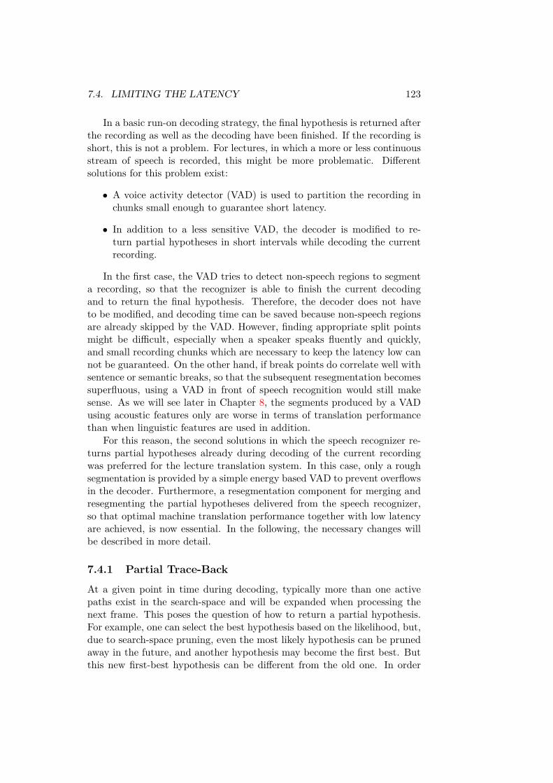
7.4. LIMITING THE LATENCY 123
In a basic run-on decoding strategy, the final hypothesis is returned afterthe recording as well as the decoding have been finished. If the recording isshort, this is not a problem. For lectures, in which a more or less continuousstream of speech is recorded, this might be more problematic. Differentsolutions for this problem exist:
• A voice activity detector (VAD) is used to partition the recording inchunks small enough to guarantee short latency.
• In addition to a less sensitive VAD, the decoder is modified to re-turn partial hypotheses in short intervals while decoding the currentrecording.
In the first case, the VAD tries to detect non-speech regions to segmenta recording, so that the recognizer is able to finish the current decodingand to return the final hypothesis. Therefore, the decoder does not haveto be modified, and decoding time can be saved because non-speech regionsare already skipped by the VAD. However, finding appropriate split pointsmight be difficult, especially when a speaker speaks fluently and quickly,and small recording chunks which are necessary to keep the latency low cannot be guaranteed. On the other hand, if break points do correlate well withsentence or semantic breaks, so that the subsequent resegmentation becomessuperfluous, using a VAD in front of speech recognition would still makesense. As we will see later in Chapter 8, the segments produced by a VADusing acoustic features only are worse in terms of translation performancethan when linguistic features are used in addition.
For this reason, the second solutions in which the speech recognizer re-turns partial hypotheses already during decoding of the current recordingwas preferred for the lecture translation system. In this case, only a roughsegmentation is provided by a simple energy based VAD to prevent overflowsin the decoder. Furthermore, a resegmentation component for merging andresegmenting the partial hypotheses delivered from the speech recognizer,so that optimal machine translation performance together with low latencyare achieved, is now essential. In the following, the necessary changes willbe described in more detail.
7.4.1 Partial Trace-Back
At a given point in time during decoding, typically more than one activepaths exist in the search-space and will be expanded when processing thenext frame. This poses the question of how to return a partial hypothesis.For example, one can select the best hypothesis based on the likelihood, but,due to search-space pruning, even the most likely hypothesis can be prunedaway in the future, and another hypothesis may become the first best. Butthis new first-best hypothesis can be different from the old one. In order

124 CHAPTER 7. LATENCY AND REAL-TIME
to prevent mis-translations in the simultaneous translation system, one hasto make sure that only those partial hypotheses are returned by the speechrecognizer which will not change in the future.
To support this, a partial trace-back mechanism was implemented in Ibis.At a given point in time during decoding, all active paths in the search-spaceare traced back, and as soon as the trace-backs become unique the wordsalong the unique path can be returned as a first-best partial hypothesis.Subsequent partial trace-backs always return the words along the uniquepath starting from the end point of the preliminary trace-back, up to thepoint where the search path diverges. Since the number of active pathsin each frame is limited – by the transN pruning parameter – the addi-tional overhead is relatively small. Unfortunately, further optimization ofthe speech recognizer’s output through lattice rescoring is no longer possi-ble. Due to edges added to the lattice after the decoding has been finished,lattice rescoring is non-linear with time.
7.4.2 Front-End and Online Adaptation
As described in Section 4.3.3, audio offset correction, cepstral mean sub-traction (CMS), and cepstral variance normalization (CVN) are performedvia global normalization over the whole utterance. But in combination withthe partial trace-back, utterance based normalization is no longer possible.Instead, normalization parameters have to be estimated from the partial hy-potheses and have to be updated incrementally. Furthermore, an additionalhistory weighting was introduced so that the normalization can adapt tochanging environmental acoustic conditions.
In order to judge the amount of data necessary for updating the normal-ization parameters and the influence on latency of the additional overhead ofthe update as well as the partial trace-back, a few experiments with differentinterval lengths were performed. As can be seen in Table 7.5, the smaller theinterval, i.e. the more often the parameters are updated based on the partialtrace-back result, the higher the overhead. While for an interval with fiveseconds a total real-time factor of 0.93 was measured, for an interval of 0.5seconds it was 1.05. The total real-time factor includes, in addition to thedecoding, also the time necessary for updating the normalization parame-ters and for the partial trace-back. Furthermore, the shorter the interval,the shorter the latency. In terms of WER, it can be seen that there is anoptimum at an interval of three seconds. Unfortunately, because of the la-tency, only intervals between one or two seconds in duration are possible.Interesting in the results is that due to the more frequent update of the nor-malization parameters, leading to a higher sensitivity against changes in theenvironmental acoustic conditions, the baseline WER can be outperformed.
The baseline is a system which uses manual segmentation and utterance-based global normalization in the front-end. No other kind of adaptation

7.4. LIMITING THE LATENCY 125
interval WER LAT RTF RTFlength decoding totalbaseline 16.9% 1.10 1.10
0.5 17.3% 3.48 1.01 1.051.0 16.7% 3.60 0.97 0.982.0 16.6% 5.10 0.95 0.963.0 16.4% 6.83 0.94 0.955.0 16.6% 10.36 0.93 0.93
Table 7.5: Comparison of the word error rate, latency in seconds, real-timefactor of the decoding itself and the total real-time factor for different audiointerval durations (in seconds) on LectDev.
was performed during decoding and no lattice rescoring was applied, for allexperiments. The baseline system is identical to the one described in Section5.3, which achieved a WER of 16.4% after lattice rescoring (see Table 5.1,column VTLN-AM).
The same changes are necessary for online adaptation. For both VTLNand cMLLR, an additional history-weighting factor has to be introduced.Table 7.6 compares the results of the baseline system using manual seg-mentation with systems using partial trace-backs after intervals of 1-2 sec-onds. As can be seen, the systems’ recognition accuracy suffers only slightly.VTLN improves the WER only slightly but does not influence latency orthe real-time factor. In contrast, cMLLR reduces the WER significantly,but the total RTF increases as well. On the other hand, the decoding is ac-celerated due to adaptation, which can be observed in the smaller decodingRTF when cMLLR is applied.
Latencies achieved for the systems using a one second interval are sig-nificantly lower than those obtained with a two second interval if the totalreal-time factor is lower than one. In the case of the system with incre-mental VTLN and cMLLR using a one second interval, it can be seen whathappens if the total real-time factor is higher than 1.0. The system cannotkeep up with the speaking rate of the input speech leading to high latency.In such cases, applying additional speed-up techniques as described aboveare essential. The results can be seen in the conclusion to this chapter.
7.4.3 Language Model
For language model training, the training corpora are traditionally split atsentence boundaries in order to be able to estimate transition probabilitiesfor words at the beginning or end of a sentence. But due to continuousprocessing of the input speech, together with a trace-back, this reformattingno longer makes sense. Therefore, in accordance with [SCER97, GLA98]

126 CHAPTER 7. LATENCY AND REAL-TIME
WER LAT RTF RTFdecoding total
baseline 16.9% 1.10 1.10+ VTLN 16.6%+ VTLN + cMLLR 15.1%1.0 16.7% 3.60 0.97 0.98+ VTLN 16.4% 3.60 0.95 0.98+ VTLN + cMLLR 15.3% 6.33 0.86 1.182.0 16.6% 5.10 0.95 0.96+ VTLN 16.3% 5.10 0.93 0.95+ VTLN + cMLLR 15.3% 5.80 0.85 1.08
Table 7.6: Comparison of the baseline system using manual segmentationwith systems using partial trace-back at intervals of 1-2 seconds of inputspeech. Results after applying VTLN as well as cMLLR are compared interms of word error rate (WER), latency (LAT) and real-time factor (RTF)on lectDev.
sentence LM continuous LMbaseline 16.9% 16.9%2.0 16.7% 16.3%
Table 7.7: Comparison of the results (WER) obtained by using a sentencelanguage model and a continuous language model with the baseline system,i.e. with manual segmentation, and a system using the partial trace-backmechanism with an interval of two seconds. All experiments were performedon lectDev.
additional n-grams across sentence boundaries were added to the languagemodel. Table 7.7 shows the improvement in WER for the continuous lan-guage model if the partial trace-back mechanism is used.
7.5 Conclusion
In this chapter it was discussed how the real-time and latency requirementsof a simultaneous lecture translation system can be fulfilled. The focuswas to speed-up the computationally most expensive component, the speechrecognition, and to introduce overlapping processing into the framework toreduce the latency.
First of all, the search space pruning technologies (relative and topN)implemented for different levels (state, linguistic, and word level) in the Ibisspeech recognition decoder were analyzed in more detail. It was investigatedhow the different pruning parameters influence the speed and accuracy of

7.5. CONCLUSION 127
WER LAT RTF RTFlectDev decoding total
baseline 4000-64 15.1% 1.14 1.203000-64 14.9% 1.14 1.20+ optimized pruning 15.2% 0.88 0.93+ Gaussian clustering 15.4% 0.65 0.701.0 15.5% 2.16 0.56 0.882.0 15.2% 3.61 0.55 0.78
Table 7.8: Final performance results after speeding-up the decoding andreducing the latency of the speech recognition on lectDev. While for the topbaseline the 4000-64 AM was used, the other results were obtained with the3000-64 AM. For the experiment with a trace-back at intervals of one ortwo seconds, all optimizations from above were used. The results are givenin word error rate (WER), latency (LAT) and real-time factor (RTF).
the decoder and how they depend on each other. Changes in the state beaminfluences the ratio between recognition accuracy and decoding speed most,followed by the word beam. The influence of the topN pruning parametersis only little. As a result of this analysis, an optimized pruning parametercombination was determined.
It was shown that although Ibis is a single pass decoder, further lan-guage model rescoring based on lattices produced during decoding improvesthe WER with only a minor increase in overall decoding time. In thiscontext, the relationship between language model parameters and pruningparameters was explained. For the 3000-64 AM, the real-time factor couldbe improved by 24% relatively to 0.88 with an increase in WER by 1.4%relative to 14.6% only.
In the next step, optimizations in the Gaussian Layer of the Ibis decoderwere investigated. Two algorithms, the Bucket Box Intersection (BBI) al-gorithm and Gaussian clustering, were compared with respect to their per-formance, i.e. decoding speed vs. accuracy. For both methods, the resultswere compared for different acoustic models and with different parametersettings. It turns out that, with appropriate tuning, Gaussian clusteringoutperforms BBI in terms of speed and accuracy. Therefore, the functionfor computing the observation probabilities was optimized to reduce theoverhead of the Gaussian clustering. Another observation was made afterdiscriminative training was applied to the acoustic models. The best resultsare now achieved with AMs using a smaller number of Gaussians. Also,the improvement in performance by using Gaussian selection for the dis-criminatively trained AMs is smaller than compared to that obtained withnon-discriminatively trained AMs.
Tables 7.8 and 7.9 summarize the results. First, the baseline system us-

128 CHAPTER 7. LATENCY AND REAL-TIME
WER LAT RTF RTFlectEval decoding total
baseline 4000-64 16.6% 1.21 1.283000-64 16.2% 1.23 1.30+ optimized pruning 16.3% 0.94 1.00+ Gaussian clustering 16.8% 0.70 0.771.0 17.0% 2.95 0.61 0.932.0 16.9% 4.30 0.60 0.83
Table 7.9: Final performance results after speeding-up the decoding andreducing the latency of the speech recognition on lectEval. While for thetop baseline the 4000-64 AM was used, the other results were obtained withthe 3000-64 AM. For the experiment with an trace-back at intervals of oneor two seconds length all optimizations from above were used. The resultsare given in word error rate (WER), latency (LAT) and real-time factor(RTF).
ing the 4000-64 acoustic model is compared to the 3000-64 acoustic model.Both are trained with MMIE and use default pruning parameters, no Gaus-sian selection, and incremental adaptation during decoding. Second, theoptimized pruning parameters were applied to the 3000-64 AM and thenGaussian clustering was used in addition. For Gaussian clustering, the best64 clusters out of 1024 were selected in each frame.
As can be seen, the 3000-64 AM performs slightly better than the 4000-64 AM at the same speed. When using the optimized pruning parametersas well as the Gaussian clustering, the real-time factor is almost halved,with an increase in WER of 3.4% on the development data and only about4.3% on the evaluation data. Furthermore, by using the partial trace-backmechanism together with the continuous language model, the latency couldbe reduced to 2-3 seconds for a one second interval and to about four secondsfor a two second interval. The latencies on the evaluation data are higherthan those on the development data, which is related to the higher WERand RTF. Due to the much lower latency, the one second interval is preferredover the two second one even if the WER is slightly worse.
Overall, a WER of 15.5% with a latency of 2.16 seconds could be achievedon the development data and a WER of 17.0% with a latency of 2.95 secondson the evaluation data. The obtained latencies hold for speech recognitiononly. In the next chapter, the interface between speech recognition andmachine translation will be explored.

Chapter 8
Translatable SpeechSegments
In speech translation systems, the combination of automatic speech recog-nition (ASR) and machine translation (MT) is not always straight forwardwhen optimal performance is the goal. For the lecture translation system, inaddition to the errors committed by the speech recognition leading to errorsin machine translation, the partial ASR hypotheses have to be resegmentedsuch that MT performance does not suffer further. Since almost all MTsystems are trained on data split at sentence boundaries, this is commonlydone by resegmenting the hypotheses according to automatically detectedsentence boundaries.
However, automatic sentence boundary detection, or punctuation anno-tation in general, is, depending on the type of data, still very challenging.Punctuation annotation is usually done by combining lexical and prosodicfeatures [Liu04], and the combination is often done with the help of maxi-mum entropy models [HZ02] or CART-style decision trees [KW01].
Within TC-STAR, Lee et al. [LAOPR06] proposed a system whichinserts commas within a given ASR sentence by using n-gram statis-tics for commas together with certain thresholds to improve MT quality.[RSM+06b] proposed another solution for inserting commas and periods intothe ASR output, by using a maximum entropy classifier using durational andlanguage model features. Using this classifiers for each contiguous non-wordsequence, it was decided if it is replaced by a comma or period. They ob-served on English a 98% correlation for periods and a 70% correlation forcommas.
In [MMN06], different approaches for automatic sentence segmentationand punctuation prediction were compared with respect to MT performance.Punctuation prediction was either done with the help of a hidden n-gram[Sto98] or by generating them implicitly during the translation process. Forsentence segmentation, an HMM-style search using hidden-events to repre-
129

130 CHAPTER 8. TRANSLATABLE SPEECH SEGMENTS
sent segment boundaries was used, extended with an additional sentencelength model. To obtain an optimal segmentation of a document, a globalsearch, restricted by the sentence length model has to be performed.
Performing a global search is also necessary for the technique describedin [XZN05], where an IBM word alignment model 1 is used, and other ap-proaches to improve example base MT, where longer sentences do not yieldgood translation performance [KZK00, DS05]. The approach in [LGCL96]splits sentences before and during parsing to improve the translation perfor-mance of an Interlingua-based MT system for Spanish-English. The aboveapproaches, however, have focused on limited domain tasks only and are noteasily extensible to more difficult domains.
For simultaneous translation systems [FKPW06], merging and chunkingof partial ASR hypotheses into useful translatable segments is even morecritical and difficult. Due to the resulting latency, a global optimization overseveral ASR hypotheses, as suggested in the approaches described above, isimpossible. Instead, the latency should be kept as small as possible asdescribed in Chapter 3.
This chapter presents and extends the work, inspired by experimentsdone by Cettolo et. al. [CF06] on investigating the impact on transla-tion performance of different text segmentation criteria, and was publishedin [FK07]. It addresses the questions of how chunking of ASR hypothe-ses as well as ASR reference transcripts into translatable segments, usuallysmaller than sentences, influences MT performance. Different segmentationstrategies on ASR hypotheses as well as on the reference transcripts arecompared. To measure the usefulness for simultaneous translation, MT per-formance was set in relation to the average segment length and its standarddeviation.
Simultaneously with [FK07], another work was published by Rao[RLS07b]. This work was aimed to improve the translation performanceby optimizing the translation segment length only, instead of reducing thesegment length to decrease translation system latency. The interesting re-sult of this work is that the best performance is achieved with segmentssmaller than sentences, similar to the observations described here.
In contrast to Chapter 4, other systems and test data were used, becausethe translation direction was from Spanish into English instead of vice versa.The reason for this was that to the time when these studies were made, theSpanish-English TC-STAR translation system achieved the best translationresults. Therefore, Section 8.1 explains the differences in more detail. Theexperimental results of this study and a new segmentation algorithm arepresented and discussed in Section 8.2. Section 8.3 concludes this chapterand shows that the obtained results can be transferred to translation oflectures in the other direction, i.e. from English into Spanish.

8.1. DATA AND SYSTEMS 131
8.1 Data and Systems
As test data, the 2006 Spanish-English TC-STAR development data, con-sisting of 3hrs (14 sessions) of non-native Spanish speech recorded at theEuropean Parliament, was selected. For this set, ASR hypotheses as wellas reference transcripts and translations were available, while the Spanishhypotheses were generated with a system trained within TC-STAR on Par-liament Plenary Sessions [SPK+07]. The case-insensitive word error ratewas 8.4%.
8.1.1 Statistical Machine Translation
The Spanish-English machine translation system [KZV+06] was trained us-ing minimum error rate training [Och03] on the same parallel EPPS data asmentioned in Section 4.4, but with the translation direction from Spanishto English. For decoding, a word reordering window size of four was used.As will be shown later, the translation quality of this system on the abovementioned data is much higher than the English-to-Spanish results on lec-tures. The reason for this is the much better match between the trainingand test data in speaking style as well as topic.
8.2 Experimental Results and Discussion
In this section, the translation scores achieved by translating ASR referencetranscripts as well as ASR hypotheses resegmented with different chunk-ing strategies are compared and discussed. Since punctuation annotationof ASR hypotheses is a research problem in itself, and not the focus of thisthesis, all punctuation marks in the reference transcripts were removed forcomparison reasons. However, the MT system was trained on complete sen-tences containing punctuation marks, since punctuation marks can provideuseful alignment boundaries during the word alignment training.
Another problem is the influence of the LM on the translation qualityof different chunking strategies. For language model training, the trainingcorpora are typically split at sentence boundaries so as to estimate the tran-sitions at the beginning and end of a sentence; chunking strategies, whichproduce segment boundaries with a high correlation to sentence boundaries,are therefore affected adversely. To mitigate this effect, the language modeltraining corpora were resegmented accordingly.
For further analysis, in addition to the translation scores and segmentlength statistics, precision and recall are computed by aligning the segmentboundaries to punctuation marks in the ASR reference transcripts.

132 CHAPTER 8. TRANSLATABLE SPEECH SEGMENTS
8.2.1 Scoring MT with Different Segmentations
The commonly used metrics for the automatic evaluation of machine trans-lation output, such as the Bleu [PRWZ02] and NIST [NIS04] metrics, haveoriginally been developed for written text, where the input segment bound-aries correspond to the reference sentence boundaries. This is not thecase for translation of spoken language where the correct segmentation intosentence-like units is unknown and must be produced automatically by thesystem.
In order to be able to use the established evaluation measures, the trans-lation output of the automatically produced segments must be mapped tothe reference translation segments in advance, before the scoring procedure.This is done by using the method described in [MLBN05], which takes advan-tage of the edit distance algorithm to produce an optimal resegmentation ofthe hypotheses for scoring, and which is invariant to the segmentation usedby the translation component.
The Bleu scores presented in this paper were obtained by using thismethod using two reference translations. Since the alignment was performedon a per-session level, the result is invariant in relation to the number ofsegments produced for a single session. The scoring was case-insensitive,without taking punctuation marks into account.
8.2.2 Baselines
Resegmenting ASR hypotheses at sentences boundaries for MT is the mostcommon approach for speech translation systems. For this reason, the trans-lation scores obtained by translating ASR hypotheses, as well as referencetranscripts split at sentence boundaries (sent), serve as one baseline for thefollowing experiments. As can be seen in Table 8.1, a Bleu score of 37.6%by translating ASR reference transcripts, and a score of 34.3% for ASRhypotheses were obtained, which clearly shows the influence of ASR perfor-mance on MT quality. The average segment length was 30 words with astandard deviation of 22.
Another baseline is obtained by taking all punctuation marks as splitpoints (punct). Here, the average segment length can be reduced to ninewords with almost no decrease in the translation score. The reason for this isthat punctuation marks are usually used to represent semantic boundaries.However, one needs to be careful because, as the use of punctuation marksdiffers from language to language, they might be impractical as split pointsfor languages other than Spanish. Note that, for both baselines, the LMtraining corpus was split accordingly.
In the following sections, it will be analyzed how MT performance isaffected by chunking strategies using other features and approaches requiringa smaller amount of context information for their decision.

8.2. EXPERIMENTAL RESULTS AND DISCUSSION 133
8.2.3 Destroying the Semantic Context
In the following experiments, it was analyzed how MT performance is af-fected by destroying the semantic context of an utterance independently ofthe applicability for simultaneous translation. Following the experimentsin [CF06] the merged utterances of a single session were simply cut everyn words (fixed). The results are given in Table 8.1 for n ∈ {7, 11, 15} andprovide a lower bound for the subsequently explored chunking strategies. Asexpected, the decrease in segment size affected the translation scores dra-matically. The translation results could be significantly improved by justcutting a sentence into two (sent-0.5) or four (sent-0.25) segments of equalsize and not splitting across sentence boundaries. This clearly shows thedependency of the MT performance on the segmentation used for trainingthe MT system.
8.2.4 Using Acoustic Features
Following the studies in [Che99] in which pauses were shown to closely corre-spond to punctuation, the information from non-speech regions in the ASRhypotheses was used for resegmentation. As non-speech regions, recognizedsilences and non-human noises were used, and successive noises and silenceswere merged together. For the translation scores (pause) in Table 8.1 differ-ent non-speech duration thresholds (0.1, 0.2, and 0.3 seconds) were selected.As expected, the results are significantly better than those obtained with thechunking strategies in Section 8.2.3. The precision and recall values clearlyvalidate the studies in [Che99], also for Spanish. While a threshold of 0.1has the best correlation to punctuation marks, the MT score is the worst.
The standard deviations of the segment lengths achieved with the non-speech chunking strategies are still too large for use in simultaneous trans-lation. By splitting the ASR hypotheses at the longest non-speech intervalwithin a region of a maximum number of words (var15, var20, var25, withchunks of maximal 15, 20, 25 words), the standard deviation could be signif-icantly reduced without decreasing the translation quality when comparingfixed and variable non-speech chunking strategies having a similar averagesegment length.
Overall, chunking strategies using non-speech regions are simple andrequire no additional context information, but nonetheless achieve relativelygood translation scores. The reason for this seems to be the relatively goodcorrelation of the split points with sentence boundaries, as can be seen inthe high precision and recall values.
8.2.5 A New Segmentation Algorithm
Given the results above, a new segmentation algorithm, suitable for the lec-ture translation system, was developed. Only lexical information, such as

134 CHAPTER 8. TRANSLATABLE SPEECH SEGMENTS
punctuation marks, filled pauses and human noises, was taken into account.At least for the languages investigated so far, using additional prosodic fea-tures has shown to be less profitable [CF98].
According to [CF98], a trigram language model was trained, in which alllexical cues in the training corpus were substituted by a boundary tag BD.Instead of doing a global optimization over the whole sentence, the decisionwas made using local information only, by (1) setting the LM probabilitiesPr(wi−1wiBDwi+1wi+2) and Pr(wi−1wiwi+1wi+2) in relation to each other;and (2) using additional thresholds for the non-speech gap in between wiand wi+1, i.e. regions in which the ASR decoder recognized a non-speechevent such as silence, a filled pause, or a human noise. Since the LM trainingdata does not contain any acoustic information, it was resegmented by usingthe lexical cues only.
As can be seen in Table 8.1 (lm) this chunking strategy outperforms allother strategies using only acoustic features. A precision of 73% and a recallof 54% were measured. However, a standard deviation of 10 from the averageof 11 words was also found. Therefore, in a second experiment the abovementioned thresholds were restricted when no split point was found afterten words (lm-10). Thereby, the standard deviation could be almost halvedwith only a minor decrease in Bleu score. Furthermore, both strategiesare slightly better than the baseline computed on sentence boundaries andalmost as good as the baseline computed on punctuation marks.
8.3 Conclusion
In this chapter, the question on how utterance chunking influences machinetranslation performance was addressed in an empirical study by comparingdifferent chunking strategies on ASR hypotheses as well as on ASR refer-ence transcripts. As can be seen in Figure 8.1, sentence boundaries are agood criterion for utterance chunking, but are inapplicable for simultaneoustranslation because of the high average sentence length. Chunking strategiesbased on non-speech regions are simple and require no additional contextinformation, achieving relatively good translation scores.
Given these results, a more sophisticated approach using lexical featuresprovided by a LM, in addition to acoustic features, was developed, whichoutperforms all chunking strategies using only acoustic features and yieldssimilar in translation quality as the baselines. Furthermore, by restrictingthe thresholds for this heuristic after 10 words (lm-10), a suitable averagesegment length for the lecture translation system of 9 with a small standarddeviation of 6 could be achieved.
Table 8.2 shows the results of the experiments, but for the other trans-lation direction, i.e from English into Spanish. Segmentations based onsentence boundaries and punctuation marks in general are compared to the

8.3. CONCLUSION 135
Chunking SegLength Correlation Bleustrategy avg sdev PRC RCL Ref ASR
Baselinesent 30.1 22.1 98.5 26.5 37.56 34.28punct 9.2 6.7 100.0 98.6 38.27 35.47
Destroying the semantic contextfixed-7 7.0 0.2 22.8 26.5 30.13 27.50fixed-11 11.0 0.7 22.6 16.8 32.07 29.53fixed-15 15.0 0.6 23.8 13.0 33.64 30.66sent-0.5 15.3 11.3 59.0 31.8 35.08sent-0.25 10.3 8.5 44.9 36.1 33.67
Using acoustic featurespause-0.1 8.2 5.7 59.3 58.3 31.86pause-0.2 12.1 11.0 66.3 44.5 32.53pause-0.3 17.0 19.6 71.5 34.0 32.62pause-var15 7.5 3.1 59.4 61.4 31.34pause-var20 9.8 4.3 64.6 53.0 31.87pause-var25 11.8 5.3 68.3 46.9 32.36
New segmentationlm 10.9 9.8 73.1 54.1 34.93lm-10 8.7 5.6 67.3 62.4 34.77
Table 8.1: Bleu scores obtained on ASR reference transcripts (Ref) as well ason ASR hypotheses (ASR) together with the average (avg) segment lengthand standard deviation (sdev). Precision (PRC) and Recall (RCL) of seg-mentation boundaries to punctuation marks are given as well.
avg sdev Bleu Bleul043 t036+t037
sent 27.1 20.2 17.7 19.9punct 11.1 9.6 18.1 19.9lm-10 10.2 6.0 18.0 20.2lm-8 8.9 4.4 18.0 19.9
Table 8.2: Comparison of the language model based segmentation (lm-10,lm-8) with segmentations at sentence boundaries (sent)and punctuationmarks (punct) for English-to-Spanish lecture translation on lectEval. Allresults are obtained on ASR hypotheses.

136 CHAPTER 8. TRANSLATABLE SPEECH SEGMENTS
20
22
24
26
28
30
32
34
36
sent punctpause-0.2
pause-var25
fixed-11lm pause-var20
lm-10pause-0.1
pause-var15
fixed-7 0
5
10
15
20
25
30Bl
eu [%
]
word
s/ se
gmen
t
baselines on ASR hypotheses [Bleu]using ASR hypotheses [Bleu]
average, standard deviation [words/ segment]
Figure 8.1: Results obtained by chunking ASR hypotheses sorted descendingaccording to their average segment length. Bleu scores (left axis) are rep-resented by boxes, the markers in the middle of the boxes give the averagesegment length (right axis) together with the standard deviation.
above-developed language model-based segmentation. As can be seen, theaverage segment length as well as the standard deviation can be significantlyreduced with the help of the language model-based segmentation (lm-10),without any degradation in translation performance. Furthermore, by re-stricting the thresholds after eight words to reduce the latency further, onlya slight degradation in translation quality was observed. It should be notedthat all results were obtained on ASR hypotheses produced with the systemdescribed in Section 7.5 using 1 second intervals for partial trace-back. Thissystem achieved a WER of 16.8% on t036, 13.7% on t037, and 16.0% onl043.

Chapter 9
A System for SimultaneousSpeech Translation
Given the description of the individual components of the simultaneoustranslation system in the previous chapters, this chapter introduces the ar-chitecture of the simultaneous translation system implemented in this thesis.Figure 9.1 shows the system as deployed in a real lecture scenario.
9.1 Architecture and Information Flow
Figure 9.2 shows a slightly extended version of the schematic overview ofthe simultaneous translation system which was given in Chapter 3. Thespeech of the lecturer is recorded with the help of a close-talk microphoneand processed by the speech recognition component. The partial hypothe-ses produced by this component are collected in the resegmentation com-ponent, for merging and re-splitting at appropriate “semantic” boundaries.The resegmented hypotheses are then transferred to one or more machinetranslation components, at least one per language pair. Different outputtechnologies may be used for presenting the translations to the audience.
All components of the simultaneous translation system are connectedtogether in a client-server framework, similar to the one described in[FWS+01]. It is designed such that several consumers can process the outputof one or more producers. Imagine for example a panel discussion instead ofa lecture situation, where multiple people are able to speak at the same time.For such a situation, the architecture makes it possible to use several speechrecognizers for processing the input signals. The different outputs are thenordered, merged and resegmented per speaker in different resegmentationcomponents, and several machine translation systems can then be used toconsume the output of the resegmentation components, and to translate itinto the different required languages. For the identification of the differentstreams and for the merging and resegmentation process, unique speaker-
137

138 CHAPTER 9. SPEECH TRANSLATION SYSTEM
Figure 9.1: Simultaneous translation of a lecture with the system imple-mented in this thesis.
Dictionary
Source
Hypothesis Translatable
Segment
Model
Source Boundary
Resegmen−
tationRecognition
Speech
Translation
Model Model
Target Language
Machine
Translation
Model
Source Acoustic
Model
Source Language
Output
Translated
Translation
Vocabulary
Audio Stream
Text
Output
(Subtitles)(Synthesis)
Spoken
Figure 9.2: Schematic overview and information flow of the simultaneoustranslation system. The main components of the system are represented bycornered boxes and the models accessed by these components by ellipses.The different output forms are represented by rounded boxes.

9.2. OUTPUT TECHNOLOGIES 139
and segment-related identifiers are used. The different translation streamsare then multiplexed for delivery by the different output technologies. Withthis set-up, the overall latency of the system can be significantly reduced insuch situations.
If required, the architecture also allows for combining the hypotheses ofseveral ASR components given the same input signal in order to improvethe recognition quality, by easily adding another consumer responsible forthe combination. The only problem for the simultaneous translation systemin this case is that the latency of the system not be affected.
9.2 Output Technologies
When offering simultaneous translation services, there is always the questionon how to deliver the translation to an audience. In the case of humaninterpreters, the translation has always been delivered in spoken form, andtypically headphones are used. An automatic system has the advantage thatthe translation can be delivered in written form also. In the following, theadvantages and disadvantages of the different transmission forms, types, andoutput devices are discussed in more detail.
9.2.1 In Written Form
One of the most prominent transmission types is presenting the translationas subtitles on a projection screen. The advantages of this transmission typeare that it is easy to implement, does not require any additional hardwareand can be presented to several people at the same time. However, as thenumber of necessary output languages increases, the clarity of the presen-tation suffers. In contrast, with display devices assigned to a single personor a small group of persons of the same mother tongue, it is possible todeliver target-oriented translations in the required language only, but it isnecessary to purchase additional hardware. The additional cost can be re-duced significantly by also supporting standard handheld devices like PDAsor cellphones, which are becoming more and more widely used.
All above mentioned output devices have the major disadvantage thatone is unable to look at the lecturer and presentation slides at the same timeas reading the translations. For this reason, heads-up display goggles (seeFigure 9.3) might be an ideal solution, because they enable the wearer tosee both the lecturer and the translation at the same time. Problematic inthis case is that equipping an audience with such a device is very expensive,and changing focus from the speaker to the translation device can becomevery tiring.
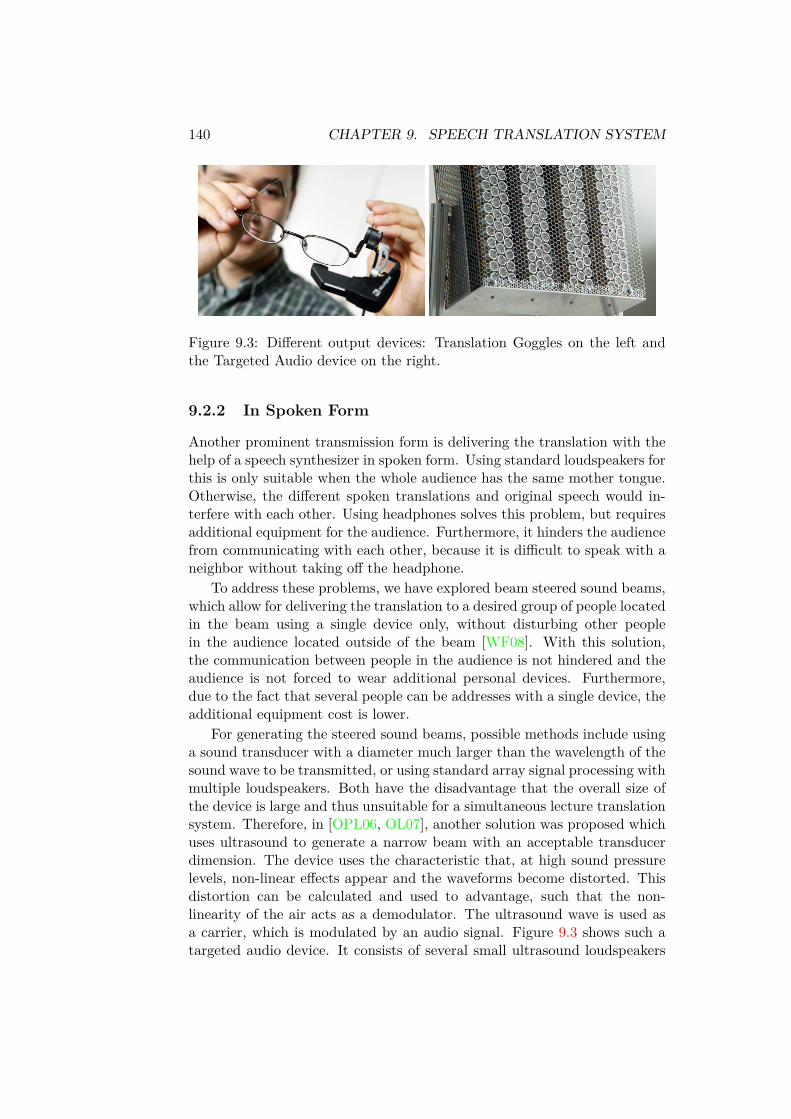
140 CHAPTER 9. SPEECH TRANSLATION SYSTEM
Figure 9.3: Different output devices: Translation Goggles on the left andthe Targeted Audio device on the right.
9.2.2 In Spoken Form
Another prominent transmission form is delivering the translation with thehelp of a speech synthesizer in spoken form. Using standard loudspeakers forthis is only suitable when the whole audience has the same mother tongue.Otherwise, the different spoken translations and original speech would in-terfere with each other. Using headphones solves this problem, but requiresadditional equipment for the audience. Furthermore, it hinders the audiencefrom communicating with each other, because it is difficult to speak with aneighbor without taking off the headphone.
To address these problems, we have explored beam steered sound beams,which allow for delivering the translation to a desired group of people locatedin the beam using a single device only, without disturbing other peoplein the audience located outside of the beam [WF08]. With this solution,the communication between people in the audience is not hindered and theaudience is not forced to wear additional personal devices. Furthermore,due to the fact that several people can be addresses with a single device, theadditional equipment cost is lower.
For generating the steered sound beams, possible methods include usinga sound transducer with a diameter much larger than the wavelength of thesound wave to be transmitted, or using standard array signal processing withmultiple loudspeakers. Both have the disadvantage that the overall size ofthe device is large and thus unsuitable for a simultaneous lecture translationsystem. Therefore, in [OPL06, OL07], another solution was proposed whichuses ultrasound to generate a narrow beam with an acceptable transducerdimension. The device uses the characteristic that, at high sound pressurelevels, non-linear effects appear and the waveforms become distorted. Thisdistortion can be calculated and used to advantage, such that the non-linearity of the air acts as a demodulator. The ultrasound wave is used asa carrier, which is modulated by an audio signal. Figure 9.3 shows such atargeted audio device. It consists of several small ultrasound loudspeakers

9.3. CONCLUSION 141
Figure 9.4: The lecture scenario.
and outputs audio in a beam of a width of about 1-2 meters.
9.3 Conclusion
Figure 9.4 shows again the lecture scenario already presented in Chapter3. The lecturer is standing between the projection screen and the audience.The audio is processed, simultaneously translated by the lecture translationsystem and delivered to the audience with the help of targeted audio devicesor heads-up display goggles. Several such targeted audio devices can beassigned to various languages to accommodate each participant in the lectureroom.
Although several problems could be solved with the help of these devices,one problem still exists, namely the delivery rate problem. To keep thelatency of the system constant, the system has to consume the input as fastas it is produced and therefore has to deliver the output with the same rate.This is especially problematic for language pairs for which an expressionwith the same meaning consists of more phonemes in the target languagethan in the source language. Figure 9.5 compares the average number ofwords in English necessary to phrase a single word of another language. Itcan be seen that e.g. a word in Finnish is phrased in almost 1.4 words inEnglish and a word in French in almost 0.9 words in English. The results

142 CHAPTER 9. SPEECH TRANSLATION SYSTEM
Figure 9.5: Comparison of the average number of words in English neces-sary to phrase a single word of another language measured on the Europarl[Koe05] corpus.
do not provide a direct comparison of the duration of a phrase in differentlanguages, because words also differ in their durations; they are meant toprovide a first impression. Furthermore, the automatic system is not perfect,and understanding an imperfectly written or spoken translation may not bean easy task. In such cases, increasing the delivery rate of the translationto keep up with the lecturer will make this task even more difficult.

Chapter 10
End-to-End Evaluation
By taking the results of the preliminary chapters into consideration, a real-time, low-latency, speaker and topic adapted English-to-Spanish simultane-ous speech-to-speech translation system was constructed.
For speech recognition, the MMIE-trained acoustic model with 184MGaussians over 3000 codebooks was adapted in a supervised manner onfour hours of speech of the same speaker (3000-64). The lectAdapt lan-guage model was adapted using a three-fold linear interpolation of (1) abackground language model, (2) a language model computed on generalspeaker-dependent topic data collected with the help of the speaker’s pastpublications, and (3) a language model computed on specific topic data re-lated to the current talk or lecture with the help of the presentation slides(re-estimated S+Ltopic lectAdapt). Where possible, the mixture weightswere optimized on reference transcripts related to the current talk; other-wise, all reference transcripts in lectOther were used instead.
To reduce system latency, decoding was performed in one second in-tervals. Between two successive intervals, incremental VTLN and cMMLRadaptation were used and partial hypotheses were returned. To improvethe real-time performance of the recognizer, Gaussian selection was appliedwhich is based on clustering all Gaussians into 1024 clusters and selectingthe top 64 clusters for each frame.
The partial hypotheses returned by the speech recognizer were re-segmented using a language model and likelihood ratio thresholds (lm-10),and then transmitted to the machine translation component.
For machine translation, the translation model was adapted using a smallnumber of manually translated lectures. For the target language model, aweb data collection was performed by using topic- and speaking style-relatedn-grams as search queries. The language models computed using the webdata as well as manually translated lectures were then interpolated with theexisting background models.
In this Chapter, automatic evaluation results of the simultaneous trans-
143
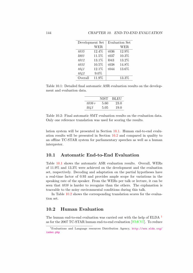
144 CHAPTER 10. END-TO-END EVALUATION
Development Set Evaluation SetWER WER
t035 12.4% t036 12.9%l003 11.5% t037 10.3%t012 13.1% l043 13.2%t032 10.5% t038 14.8%t041 12.1% t044 13.6%t042 9.0%Overall 11.9% 13.3%
Table 10.1: Detailed final automatic ASR evaluation results on the develop-ment and evaluation data.
NIST BLEUt036+ 5.60 23.0l043 5.05 19.0
Table 10.2: Final automatic SMT evaluation results on the evaluation data.Only one reference translation was used for scoring the results.
lation system will be presented in Section 10.1. Human end-to-end evalu-ation results will be presented in Section 10.2 and compared in quality toan offline TC-STAR system for parliamentary speeches as well as a humaninterpreter.
10.1 Automatic End-to-End EvaluationTable 10.1 shows the automatic ASR evaluation results. Overall, WERsof 11.9% and 13.3% were achieved on the development and the evaluationset, respectively. Decoding and adaptation on the partial hypotheses havea real-time factor of 0.93 and provides ample scope for variations in thespeaking rate of the speaker. From the WERs per talk or lecture, it can beseen that t038 is harder to recognize than the others. The explanation istraceable to the noisy environmental conditions during this talk.
In Table 10.2 shows the corresponding translation scores for the evalua-tion set.
10.2 Human EvaluationThe human end-to-end evaluation was carried out with the help of ELDA 1
as for the 2007 TC-STAR human end-to-end evaluation [HMC07]. To reduce1Evaluations and Language resources Distribution Agency, http://www.elda.org/
index.php

10.2. HUMAN EVALUATION 145
the overall effort and costs, six excerpts were used, three from each of thetwo talks t036+ and l043 of about 6 minutes each. The excerpts focus ondifferent topics each and represent a total of about 36 minutes and 7,200words. A professional human interpreter was asked to translate the samesix excerpts, and the synthesized outputs of the automatic system and thehuman interpretation were then presented to human judges.
The evaluation was split into two parts. In the component evaluation,judges were able to directly compare the source excerpts and their transla-tion. In the end-to-end evaluation, they were able to listen to the spokentranslation of the excerpts only. It should be mentioned that the judgesused for the first part of the evaluation were not used for the second part inorder to prevent biased results. For both parts, the excerpts were evaluatedin two categories: fluency and adequacy.
10.2.1 Component Evaluation
For this evaluation, 10 judges were recruited, of which 5 did not have specificknowledge of the domain of the lectures. All were Spanish native speakers.Each judge evaluated all six excerpts, and each segment was thus evaluatedby 10 different judges. The judgments were made on a per-segment level,with the segmentation carried over from the manual transcriptions of theexcerpts in the source language. As a result, segments could contain morethan one sentence. There were about 247 segments in all.
Fluency was evaluated by judging the quality equated with the syntac-tical correctness of the segment. Adequacy referred to whether the meaningof a sentence in the source language was correctly transferred into the targetlanguage. In both cases, judgment was on a five-point scale, with a value ofone for lowest and a value of five for highest quality.
Results
Table 10.3 shows the detailed automatic evaluation results of the translatedoutput restricted to the excerpts. The overall word error rate of the ASRcomponent was 11.9% with an OOV-rate of about 0.5%. On this output, theSMT achieved an overall BLEU score of about 28.94. Compared to the TC-STAR-07 system, it can be seen that there is a significant difference for bothASR and SMT performance. However, it should be kept in mind that (1)European Parliament Plenary Sessions are less difficult to recognize than lec-tures and (2) the simultaneous translation system runs in real-time, whereasthe TC-STAR-07 translation system process the data offline in many timesslower than real-time. Furthermore, it can be observed that l043 is moredifficult than t036+. This is due to the differences in topic between the twolectures, and lower coverage of the language and translation models.

146 CHAPTER 10. END-TO-END EVALUATION
ASR SMTWER BLEU NIST
l043-1 14.6% 25.62 6.30l043-2 14.5% 22.60 6.30l043-3 9.6% 28.73 7.14t036+1 11.4% 34.46 7.94t036+2 12.1% 29.41 7.19t036+3 9.2% 35.17 7.83Overall 11.9% 28.94 7.07TC-STAR-07 6.9% 40.6 9.19
Table 10.3: ASR and SMT automatic evaluation results restricted to theexcerpts used for human evaluation. Two reference translations were usedto evaluate MT performance. The last row shows the offline results of thefinal TC-STAR-07 system on different data.
all judges experts non-expertsFluency 3.13 2.84 3.42Adequacy 3.26 3.21 3.31
Table 10.4: Averaged fluency and adequacy results for the human componentevaluation.
Table 10.4 shows the averaged results for the adequacy and fluency judg-ments over all excerpts. Surprisingly, the results are lower for the expertsthan for the non-experts. A possible explanation could be that experts knowthe scientific vocabulary and are therefore more exigent. Another observa-tion is that the adequacy score is higher than the fluency score, i.e. thesimultaneous translation system is better in transferring the meaning thanensuring syntactic correctness.
10.2.2 End-to-End Evaluation
For this evaluation, 20 judges had to be recruited because of the additionalevaluation of the human interpreter result. Again, the same demands weremade on the judges as for the component evaluations, and each judge eval-uated either all six automatic or all six human excerpts.
Since judges were able to listen to the audio only, fluency was evaluatedby asking the judges to rate the overall quality of the current audio sample.It should be noted, that in contrast to the component evaluation, the qualityof the human or synthetic speech was taken into account. The judgment wason a five-point scale, reaching from one for very bad and unusable up to 5for very useful. Due to the lack of the source speech, a comprehensionquestionnaire was used for evaluating adequacy.

10.2. HUMAN EVALUATION 147
For each excerpt, the questionnaire consisted of 10 questions. Threetypes of questions were asked: simple factual (70%), yes/ no (20%), and list(10%). This was done in order to diversify the difficulty of the questionsand to test the system on different levels. The questionnaires used for eachexcerpt can be found in Appendix A.
The excerpts were presented to the judges via an online interface togetherwith the following evaluation instructions:
• listen to the excerpts only once
• answer the comprehension questionnaire
• judge the fluency
• go to the next excerpt
After evaluation, an objective verification or validation of the answerswas performed by comparing the judges’ answers with references. In order toidentify where information was lost, the SMT, ASR and interpreter outputwas analyzed in more detail. For this purpose the following voting schemewas used:
0: the information or answer is totally missing
1: the information or answer is partially correct, but clearly incompleted
2: the information or answer is really close, but does not correspond exactlyto the reference
3: the information or answer is undeniably correct
For further processing, the values where mapped to a binary scale, i.e. 0and 1 was mapped to 0, and 2 and 3 were mapped to 1.
Results
Table 10.5 shows that while the fluency of the simultaneous translationsystem was judged to be slightly better than of the TC-STAR-07 system,the fluency of human interpreters is worse on the Lectures than on the EPPStask. This is most likely due to the more spontaneous speaking style oflectures and a higher familiarity of interpreters with the topics and thetypical expressions used in the European Parliament.
Table 10.6 shows the percentage of good answers to the questionnairesgiven by judges from the output of interpreters and of the automatic sys-tems. Both automatic systems perform worse than the interpreters, and thesimultaneous translation system is worse than the TC-STAR system. Thisis clearly in accordance with the differences in WER and Bleu between theTC-STAR-07 and Lecture systems.

148 CHAPTER 10. END-TO-END EVALUATION
interpreter automatic systemTC-STAR-07 4.03 2.05Lectures 3.03 2.35
Table 10.5: Human Evaluation, Overall Fluency (1 low - 5 better).
interpreter automatic systemTC-STAR-07 0.74 0.64Lectures 0.74 0.52
Table 10.6: Human Evaluation, Overall Comprehension (0 low - 1 better).
In addition, an objective verification of the presence of the informa-tion needed for answering the questions was performed by a native Spanishspeaker. Table 10.7 shows the percentage of answers present or the maxi-mum number of answers found in the Spanish translation output and in theintermediate outputs of the ASR and SMT components. The comparisonshows that for the lecture task, the human interpreter was able to retain85% of the information needed to answer all questions, while the judges,who could listen to the interpreter output only once, then could answer 74%of the questions. The automatic system presented 58% of the necessary in-formation to the judges who then answered 52% of the questions correctly;the ASR component loses 17% of the information, compared to 3% in theTC-STAR system.
To objectively compare the translation quality of the automatic systemwith the quality of the human interpreter, the results were limited to thequestions for which the answers were included in the interpreter’s speech asshown in Table 10.8. It can be seen that in this subset the interpreters arefar better than they do over all data (from 0.74 to 0.80); this is also trueto a smaller extent for the automatic systems (from 0.64 to 0.66 and from0.52 to 0.53). However, as noted earlier there is already a loss of 20% in theASR component.
interpreter automatic system SMT ASRTC-STAR-07 0.91 0.89 0.92 0.97Lectures 0.85 0.58 0.65 0.83
Table 10.7: Human Evaluation, Objective Comprehension (0 low - 1 better).

10.2. HUMAN EVALUATION 149
interpreter automatic system TTS SMT ASRTC-STAR-07 0.80 0.66 0.91 0.93 0.97Lectures 0.80 0.53 0.60 0.70 0.80
Table 10.8: Human Evaluation, Limited Comprehension (0 low - 1 better).

150 CHAPTER 10. END-TO-END EVALUATION

Chapter 11
Conclusions
This thesis presented the first available prototype of a simultaneous speech-to-speech translation system particularly suited for lectures, speeches andother talks. It demonstrated how such a complex system can be build as wellas the limitations of the current state-of-the-art. It compares and studiesdifferent technologies to meet the given constraints in real-time, latency aswell as translation quality. With the help of this thesis one should be ableto build such a system and to make an informed analysis of anticipatedperformance versus cost of the techniques presented.
The proposed simultaneous translation system consists of two main com-ponents, the automatic speech recognition and the statistical machine trans-lation component. To meet the given constraints in latency and real-timewithout a drop in translation quality, several optimizations are necessary.The most obvious is to use adaptation. Within the proposed adaptationframework it is possible to apply adaptation on different levels, dependingon the type of information available. Different speaker and topic adaptationtechniques were studied with respect to the type and amount of data onhand. To reduce the latency of the system, different speed-up techniqueswere investigated. The interface between speech recognition and machinetranslation components was optimized to meet the given latency constraintswith the help of a separate resegmentation component.
In the automatic end-to-end evaluation, the system showed an overallword error rate of 11.9% and a BLEU score of 28.94 on the six excerpts usedfor human evaluation. This is still rather low compared to an offline systemfor translating European parliament speeches (TC-STAR-07 ). However theoffline system had no latency constraints, and parliament speeches are mucheasier to recognize and translate than compared to the more spontaneouslectures on which this thesis focuses. This clearly shows the difficulty ofthe whole task. However, the human end-to-end evaluation of the systemin which the system is compared with human interpretation shows that thecurrent translation quality allows for understanding of at least half of the
151

152 CHAPTER 11. CONCLUSIONS
content of a talk.
11.1 Thesis Results
In this thesis, different technologies required for implementing a simulta-neous translation system are analyzed. The experiments presented in thisthesis show that a satisfactory simultaneous translation system can be de-veloped with current state-of-the-art technologies. Specifically, the followingresults, summarized in Table 11.1 for speech recognition, Table 11.2 for ma-chine translation, and Table 11.3 for the resegmentation component, wereachieved. Although word error rates are given for lectDev as well, the worderror rates, real-time factors and relative improvements presented in the textbelow refer to lectEval.
Latency and Real-Time: An extensive study of the pruning parametersavailable in the Ibis decoder was carried out, which gave valuable in-sights on the influence of these parameters on recognition accuracy anddecoding speed. Changes in the state beam have the larges impact onthe ratio between recognition accuracy and decoding speed, followedby the word beam. The influence of the topN pruning parameters issmall.
In addition, it was shown that with an improved implementation,Gaussian clustering has a better WER-to-RTF ratio than Gaussianselection using the Bucket Box Intersection algorithm. This is espe-cially true if discriminative training was used for the acoustic model.Using these speed-ups, together with a smaller acoustic model, thereal-time factor was reduced from 1.28 by 40% to 0.87 with only aminor increase in WER of 1.2% (Table 11.1).
To reduce the overall latency, the output of the speech recognitioncomponent was streamed. A partial trace-back mechanism was im-plemented with which partial hypotheses can be returned in shortintervals of one or two seconds. The overall latency could be reducedfrom a few seconds to only about two seconds. Although the overheadincreases with shorter intervals, the speech recognition component hasa real-time factor of 0.93. This gives ample scope for variations in thespeaking rate.
Speaker Adaptation: Speaker adaptation was successfully applied to thelecture translation system. The impact in WER was analyzed for dif-ferent amounts of data, either in the form of reference or automatictranscripts. With 15 minutes of data – a common speaking time forpresentations – the WER could be reduced by 6.5% if reference tran-scripts were used for updating the parameters of VTLN and MLLR. In

11.1. THESIS RESULTS 153
lectDev lectEvalWER WER total RTF
baseline 4000-64 15.1% 16.6% 1.28Latency and Real-time
+ AM optimization + speed-ups 15.4% 16.8% 0.77+ reduced latency (1sec intervals) 15.2% 16.9% 0.93
Speaker Adaptation+ unsupervised AM adapt. (15min) 14.3% 16.0%+ supervised AM adapt. (15min) 14.3% 15.8%+ unsupervised AM adapt. (4hrs) 13.5% 15.3%+ supervised AM adapt. (4hrs) 12.8% 14.5%
Topic Adaptationunsup. AM + lectBase (15min) 14.3% 16.0%+ re-est. S+Ltopic 14.0% 15.5%sup. AM + lectBase (15min) 14.4% 15.6%+ re-est. S+Ltopic 13.8% 15.1%unsup. AM + lectBase (4hrs) 13.4% 14.9%+ re-est. S+Ltopic 13.0% 14.6%sup. AM + lectBase (4hrs) 12.7% 14.0%+ re-est. S+Ltopic 12.1% 13.7%unsup. AM + lectAdapt (15min) 13.6% 15.2%+ re-est. S+Ltopic 13.7% 15.1%sup. AM + lectAdapt (15min) 13.6% 15.0%+ re-est. S+Ltopic 13.5% 14.7%unsup. AM + lectAdapt (4hrs) 12.8% 14.4%+ re-est. S+Ltopic 12.8% 14.3%sup. AM + lectAdapt (4hrs) 12.1% 13.6%+ re-est. S+Ltopic 11.9% 13.3%
Table 11.1: Summarization of different techniques applied to the speech rec-ognizer in order to reduce the latency and real-time and to increase the recog-nition quality. In rows labeled with unsupervised (unsup.), ASR hypotheseswere used for offline acoustic model adaptation as well as for optimizingthe language model mixture coefficients. In rows labeled with supervised(sup.), reference transcripts were used instead. The amount of data used foradaptation is given in parentheses.
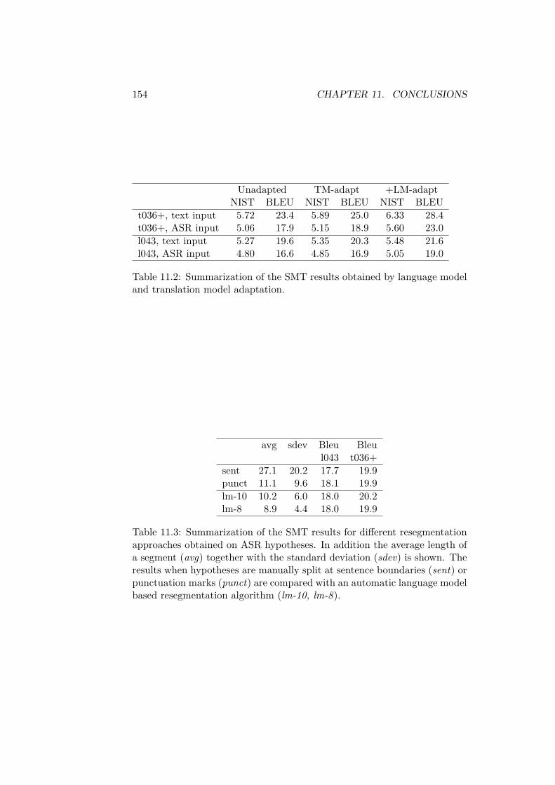
154 CHAPTER 11. CONCLUSIONS
Unadapted TM-adapt +LM-adaptNIST BLEU NIST BLEU NIST BLEU
t036+, text input 5.72 23.4 5.89 25.0 6.33 28.4t036+, ASR input 5.06 17.9 5.15 18.9 5.60 23.0l043, text input 5.27 19.6 5.35 20.3 5.48 21.6l043, ASR input 4.80 16.6 4.85 16.9 5.05 19.0
Table 11.2: Summarization of the SMT results obtained by language modeland translation model adaptation.
avg sdev Bleu Bleul043 t036+
sent 27.1 20.2 17.7 19.9punct 11.1 9.6 18.1 19.9lm-10 10.2 6.0 18.0 20.2lm-8 8.9 4.4 18.0 19.9
Table 11.3: Summarization of the SMT results for different resegmentationapproaches obtained on ASR hypotheses. In addition the average length ofa segment (avg) together with the standard deviation (sdev) is shown. Theresults when hypotheses are manually split at sentence boundaries (sent) orpunctuation marks (punct) are compared with an automatic language modelbased resegmentation algorithm (lm-10, lm-8).

11.1. THESIS RESULTS 155
the presence of four hours of data, the speed-optimized system couldeven be improved by 14.2% (from 16.9% to 14.5%). For the simulta-neous translation system, the unsupervised adaptation results are ofparticular interest. The reason for this is that unsupervised adapta-tion can be performed automatically by using hypotheses of past talksfrom the translation system itself. The WER difference when usingfour hours of speech of the same speaker is 0.7% absolute, and 0.2%absolute for only 15 minutes of speech.It was shown that even an acoustic model adapted using supervisedmethods can be further improved by using additional online adapta-tion.A speaker clustering algorithm was presented, which is based on thecMLLR parameters used during system training, and with which theadaptation parameters for online cMLLR and VTLN adaptation weresuccessfully initialized. It was shown that the recognition accuracycan be significantly improved on the first few utterances of a givenspeaker, especially for speaker-adaptively trained acoustic models.
Topic Adaptation: An adaptation framework for lectures and speecheswas presented, which allows for a fully automatic adaptation of thesimultaneous translation system towards specific topics of new pre-sentations. It was shown that queries generated using a tf-idf basedheuristic, can be successfully used to collect web data related to a spe-cific talk or lecture. The impact of general data, collected with queriesextracted from several publications of the speaker, was compared to amore specific collection with queries extracted from presentation slides.It was shown that both corpora are important and that improvementsin WER up to 4-5% relative can be expected by using both, dependingon the background language model (Table 6.16).When other lectures of the same speaker become available, they can beused for a more specific optimization of the language model mixturecoefficients as well as for background language model optimization.With the proposed adaptation framework, even a highly adapted lan-guage model (lectAdapt) can be improved by 2.2% in WER. Supervisedadaptation was compared with unsupervised adaptation. When usingwith the same acoustic model, the difference in WER is at most 1.3%(see Table 6.16). When used together with an acoustic model adaptedusing unsupervised methods, the overall improvement in WER for thebest-performing systems is 6.2% relative with lectBase and 7% rela-tive with lectAdapt. Overall, the best word error rate of 13.3% wasachieved with a speech recognizer adapted using supervised methods,with lectAdapt as a background language model.The problem of vocabulary adaptation by adding new words extracted

156 CHAPTER 11. CONCLUSIONS
from the speakers publications or from presentation slides was alsoaddressed. Although the OOV-Rate was significantly reduced by 35%relative, these improvements did not materialize in the WER (Table6.16).
For machine translation, a system trained mainly on European Parlia-ment speeches was used and successfully adapted towards the lecturedomain. First, the translation model was adapted by using other lec-ture data and by adding hand-crafted common expressions, yieldingan improvement of 2%-5% in BLEU. After this, the developed tf-idf -based web data collection was applied to the target language model.By using the collected data in addition to other lecture data, the trans-lation score (BLEU) was improved by an additional 12%-21% (Table11.2).
Resegmentation: To prepare and optimize the stream of words returnedby the speech recognition component for machine translation, a re-segmentation component was developed which tries to find semanticboundaries with the help of a statistical heuristic. It was shown thatwith this heuristic, using likelihood ratio thresholds on n-grams, theaverage segment length for English-Spanish translation systems can bekept around nine words with no increase in translation quality (Table11.3). Nine words typically correspond to an ear-voice-span of around4.5 seconds, and is similar to the ear-voice-span achieved by humaninterpreters for the investigated language pair English-Spanish.
Translation Delivery: Different ways were explored on how text or speechtranslation can be delivered to the audience. While head-phones arethe most commonly used technique, innovative devices like targetedultra-sound loudspeakers offer interesting alternatives.
Human Evaluation: Human evaluation of the system showed that, incomparison with the TC-STAR-07 offline system evaluated on par-liament speeches and the translation results of a human interpreter,the system implemented in this thesis performs worse, but still quitewell. In fluency, the simultaneous translation system was evaluatedbetter than the TC-STAR-07 system, but worse than a human in-terpreter (2.35 vs. 3.03) (see Table 11.4). However, even the latteris only average on the used scale of 1-5. The reason for this is thetechnical nature and spontaneity of the lectures and talks. In termsof comprehension, the simultaneous translation system was judged tobe 53%, which is smaller than the 66% of the TC-STAR-07 system.The human interpreters achieved 80%. It was shown that more thanhalf of the questions could be answered correctly. When the resultsof the simultaneous translation system are analyzed in more detail,

11.2. THESIS CONTRIBUTION 157
interpreter automatic system TTS SLT ASROverall Fluency (1 low - 5 better)
TC-STAR-07 4.03 2.05Lectures 3.03 2.35
Limited Comprehension (0 low - 1 better)TC-STAR-07 0.80 0.66 0.91 0.93 0.97Lectures 0.80 0.53 0.60 0.70 0.80
Table 11.4: Summary of the human evaluation results.
20% of the errors are contributed by the speech recognition compo-nent, an additional 10% by machine translation, and a further 10% toproblems in speech synthesis (Table 11.4). Note that the developmentand optimization of a speech synthesis component was not part of thisthesis.
Overall, the WER could be improved by almost 20% for an ASR systemadapted using supervised methods compared to the baseline. For a speechrecognizer adapted using unsupervised methods, the improvement was al-most 14%. At the same time, the real-time factor was reduced by 27%relative. The improvement in translation quality was about 17% on aver-age, compared to an unadapted system. The resegmented partial hypothesesof the best-performing ASR were used as SMT input.
11.2 Thesis Contribution
The experiments presented in this thesis lead to the following conclusions:
• With the final system, it is possible to understand at least half ofthe content of a simultaneously translated presentation. For a listenerwho is not able to understand the language of the speaker at all, thisis quite helpful.
• The developed adaptation framework allows the system to automati-cally adapt to a specific speaker or topic. Performance improves asspeakers continue using the system. Manually added information,such as publications, special terms and expressions, or transcripts ormanuscripts of the presentation, definitely improve adaptation perfor-mance. The performance difference between automatically and man-ually generated information is larger when more data is available.
• The adaptation framework reduces the amount of time necessary fortailoring the lecture translation system towards a specific domain. Ageneral domain-dependent language model can be adapted with the

158 CHAPTER 11. CONCLUSIONS
help of the adaptation schema implemented in this thesis, such thatit performs similarly to a highly adapted language model using hugeamounts of additional data.
• With the help of the studies about different adaptation techniques,speed-up techniques, and techniques for reducing the latency of thesystem, one can make an informed analysis of anticipated performanceversus cost of the techniques presented.
• With respect to a human interpreter, the automatic system has theadvantage that once it is adapted, it can be re-used relative cheaply.
• Interpreting is a very complex task for humans, and it is recommendedto exchange interpreters at least every half an hour. Therefore, thesimultaneous translation system is especially suitable for longer presen-tations such as lectures, or situations which are stressful for humans,such as environments with high background noise.
• The automatic system has no memory limitations. This means thatfor speakers with a high speaking rate, or when complicated sentencestructures are used, the automatic system can be advantageous overa human interpreter. In such situations, the automatic system willdefinitely not drop information, instead, the latency will increase.
• The developed client-server framework allows to easily add new pro-ducers or consumers and therefore allows to easily tailor the systemto the needs of different applications. For eaxample, multiple trans-lations can be produced at the same time by just connecting severaldifferent translation components.
At the current time, automatic simultaneous translation is not used be-cause it yields lower translation quality than a human interpreter. However,adoption depends on the cost-benefit ratio. In the authors opinion, in somesituations such as small conferences or at universities such a system may beuseful at the current performance level.
A first version of the system was presented in a press conference inOctober 2005 as well as at Interspeech 2006, where it was awarded as the“Best Presentation”.
11.3 Recommendations for Future Work
The present work represents the first available prototype of a simultaneoustranslation system. Several aspects of the system have been analyzed anddiscussed, and the available prototype reveals new problems and allows forfurther studies.
11.3. RECOMMENDATIONS FOR FUTURE WORK 159
• In the author’s opinion, the most important improvement of the si-multaneous translation system would be to port the streaming ap-proach used in speech recognition to machine translation. Althoughsegmentation in the form of inserting punctuation marks would still benecessary to increase the understandability of the output, a separateresegmentation component would be superfluous.One possibility for achieving this is to use systems based on finitestate transducers (FST) such as [SBH06]. The theory of FSTs allowsto merge the different systems into a single one so that global optimiza-tions with respect to the overall translation quality, real-time behaviorand latency can be applied.
• As seen in the human evaluation results, the performance of the ASRsystem is one bottleneck of the simultaneous translation system. Toimprove ASR performance common techniques such as lattice rescor-ing and consensus decoding should be ported to work in the streamingframework. The result of the ASR should be annotated with confi-dences to allow for more flexibility in translation.
• The support of multilinguality is another aspect which should be ad-dressed. Especially in technical talks, many expressions may be inEnglish while the rest of the talk is given in another language. A mul-tilingual acoustic model is indispensable for recognizing multilingualexpressions.
• Technical terms cannot be recognized if the corresponding words arenot included in the vocabulary. Although the developed heuristic cansignificantly reduce the OOV-Rate, the words are not added in anoptimal manner. The vocabulary adaptation can be improved to allowfor the addition or exchange of even a larger amount of new words.In this context, it may be a good idea to allow for adaptation of themachine translation component. New expressions may sometimes beincorrectly translated with the existing system.
• Currently, the stream of words returned by the speech-recognitioncomponent is translated word-by-word, and only some disfluencies arefiltered out. To improve the translation quality, an additional sum-marization component prior to translation may be a good idea, whichalso removes more complicate disfluencies and simplifies complicatedsentence structures. Moreover, depending on the summarization level,the latency of the system can also be reduced.
• Unfortunately, an alignment of slides to the recorded presentationswas not available. Motivated by results published by others, the au-thor believes that this information can improve overall system perfor-

160 CHAPTER 11. CONCLUSIONS
mance. The recognition of words and expressions found on slides canbe boosted to achieve a better recognition and translation.
• The presented output devices show interesting possibilities in deliver-ing spoken translation. Further studies and development are necessaryuntil these devices can exploit their full potential.

Bibliography
[AHH96] F. Alleva, X. Huang, and M.-Y. Hwang. Improvements of thePronunciation Prefix Tree Search Organization. In Proc. ofthe International Conference on Acoustics, Speech, and SignalProcessing (ICASSP), Atlanta, USA, 1996.
[AKC94] Andreas Andreou, Terri Kamm, and Jordan Cohen. Exper-iments in vocal tract normalization. In Proc. of the CAIPWorkshop: Frontiers in Speech Recognition II, 1994.
[AKESH00] Rajai Al-Khanji, Said El-Shiyab, and Riyadh Hussein. On theUse of Compensatory Strategies in Simultaneous Interpreta-tion. Meta : Journal des traducteurs, 45(3):544–557, 2000.
[AKMS94] Tasos Anastasakos, Francis Kubala, John Makhoul, andRichard Schwartz. Adaptation to new microphones using tied-mixture normalization. In Proc. of the International Confer-ence on Acoustics, Speech, and Signal Processing (ICASSP),pages 433–436, Adelaide, Australia, 1994. IEEE.
[AMSM96] Tasos Anastasakos, John McDonough, Richard Schwartz, andJohn Makhoul. A compact model for speaker-adaptive train-ing. In Proc. of the International Conference on Speech andLanguage Processing (ICSLP), pages 1137–1140, Philadelphia,PA, USA, 1996. ISCA.
[Aub99] X. Aubert. One Pass Cross Word Decoding for Large Vocabu-laries based on a Lexical Tree Search Organization. In Proc. ofthe European Conference on Speech Communication and Tech-nology (EUROSPEECH), Budapest, Hungary, 1999.
[Avi02] Edward Avis. Respell Version 0.1. http://membled.com/work/apps/respell/, 2002.
[Bar69] H. C. Barik. A Study of Simultaneous Interpretation. PhDthesis, University of North Carolina at Chapel Hill, 1969.
161
162 BIBLIOGRAPHY
[BBFK05] K. Bain, S. Basson, A. Faisman, and D. Kanevsky. Acces-sibility, transcription, and access everywhere. IBM SystemsJournal, 44(3):589–603, 2005.
[Bel00] Jerome R. Bellegarda. Exploiting latent semantic informationin statistical language modeling. IEEE Transactions on Acous-tics, Speech, and Signal Porcessing, 88(8):63–75, August 2000.
[Bel04] Jerome R. Bellegarda. Statistical Language Model Adaptation:Review and Persepectives. Speech Communication, 42:93–108,2004.
[Ben75] J. L. Bentley. Multidimensional binary search trees used forassociative searching. Communications of the Association forComputing Machinery, 18(9):509–517, Sep 1975.
[Boc93] E. Bocchieri. Vector Quantization for the effizient computa-tion of continuous density likelihood. In Proc. of the Interna-tional Conference on Acoustics, Speech, and Signal Processing(ICASSP), pages 692–694, Minneapolis, USA, 1993. IEEE.
[BOS03] I. Bulyko, M. Ostendorf, and A. Stolcke. Getting more Mileagefrom Web Text Sources for Conversational Speech LanguageModeling using Class-Dependent Mixtures. In Proc. HLT-NAACL, 2003.
[BT97] A. W. Black and P. A. Taylor. The Festival Speech SynthesisSystem: System documentation. Technical Report HCRC/TR-83, Human Communciation Research Centre, University of Ed-inburgh, Edinburgh, Scotland, United Kongdom, 1997. http://www.cstr.ed.ac.uk/projects/festival.
[CAB+05] Jean Carletta, Simone Ashby, Sebastien Bourban, MikeFlynn, Mael Guillemot, Thomas Hain, Jaroslav Kadlec, VasilisKaraiskos, Wessel Kraaij, Melissa Kronenthal, GuillaumeLathoud, Mike Lincoln, Agnes Lisowska, Iain McCowan, Wil-fried Post, Dennis Reidsma, and Pierre Wellner. The AMImeeting corpus: A Pre-Announcement. In Machine Learningfor Multimodal Interaction: Second International Workshop,MLMI 2005, pages 28–39, Edinburgh, UK, 2005.
[CBF04] M. Cettolo, F. Brugnara, and M. Federico. Advances in theAutomatic Transcription of Lectures. In Proc. of the Interna-tional Conference on Acoustics, Speech, and Signal Processing(ICASSP), Montreal, Canada, 2004.

BIBLIOGRAPHY 163
[CF98] M. Cettolo and D. Falavigna. Automatic Detection of Seman-tic Boundaries based on Acoutic and Lexical Knowledge. InProc. of the International Conference on Speech and LanguageProcessing (ICSLP), Sidney, Australia, 1998.
[CF06] M. Cettolo and M. Federico. Text Segmentation Criteria forStatistical Machine Translation. In FinTAL – 5th InternationalConference on Natural Language Processing, LNCS, pages 664– 673, Turku, Finland, 2006. Springer Verlag Berlin/ Heidel-berg.
[CG98] S. F. Chen and J. Goodman. An Empirical Study of SmoothingTechniques for Language Modeling. Technical Report TR-10-98, Computer Science Group, Harvard University, Cambridge,MA, USA, 1998.
[Che99] C. Chen. Speech Recognition wiht Automatic Punctuation. InProc. of the European Conference on Speech Communicationand Technology (EUROSPEECH), Budapest, Hungary, 1999.
[CMU] The CMU Pronunciation Dictionary v0.6. http://www.speech.cs.cmu.edu/cgi-bin/cmudict.
[Cona] Linguistic Data Consortium. English Broadcast NewsSpeech. http://www.ldc.upenn.edu. catalog IDs LDC97S44,LDC98S71.
[Conb] Linguistic Data Consortium. English Gigaword. http://www.ldc.upenn.edu. catalog ID LDC2003T05.
[Conc] Linguistic Data Consortium. Hansard French/English. http://www.ldc.upenn.edu. catalog ID LDC95T20.
[Cond] Linguistic Data Consortium. Translanguage English Database(TED) Speech. http://www.ldc.upenn.edu. catalog IDLDC2002S04.
[Cone] Linguistic Data Consortium. UN Parallel Text. http://www.ldc.upenn.edu. catalog ID LDC94T4A.
[Con04] Linguistic Data Consortium. ICSI, ISL and NIST MeetingSpeech Coprora at LDC. http://www.ldc.upenn.edu, 2004.catalog IDs LDC2004S02, LDC2004S05, LDC2004S09.
[CSMR04] Arthur Chan, Jahanzeb Sherwani, Ravishankar Mosur, andAlex Rudnicky. Four-Layer Categorization Scheme of Fast

164 BIBLIOGRAPHY
GMM Computation Techniques in Large Vocabulary Con-tinuous Speech Recognition Systems. In Proc. of the In-ternational Conference on Speech and Language Processing(INTERSPEECH), pages 689–692, Jeju Island, Korea, 2004.ISCA.
[Dir07a] Directorate-General for Interpretation. What we do –FAQ. http://scic.cec.eu.int/europa/display.jsp?id=c_5204, 2007. Online accessed 20-June-2007.
[Dir07b] Directorate-General for Translation. Translating for a Multilin-gual Community. http://ec.europa.eu/dgs/translation/bookshelf/brochure_en.pdf, 2007. Online accessed 20-June-2007.
[Dir07c] Directorate-General for Translation. Translation Toolsand Workflow. http://ec.europa.eu/dgs/translation/bookshelf/tools_and_workflow_en.pdf, 2007. Online ac-cessed 20-June-2007.
[Dod02] George Doddington. Automatic Evaluation of Machine Trans-lation Quality Using N-gram Co-Occurence Statistics. Tech-nical report, NIST, 2002. http://www.nist.gov/speech/tests/mt/doc/ngram-study.pdf.
[DS05] Takao Doi and Eiichiro Sumita. Splitting Input for MachineTranslation Using N-gram Language Model together with Ut-terance Similarity. IEICE Transactions on Information andSystems, 88(6):1256–1264, June 2005.
[Eur] The European Parliament Online. http://www.europarl.europa.eu.
[FA07] Jonathan Fiscus and Jerome Ajot. The Rich Transcrip-tion 2007 Speech-to-Text (STT) and Speaker AttributedSTT (SASTT) Results. In Rich Transcription 2007 Meet-ing Recognition Workshop, Baltimore, MD, USA, May2007. NIST. http://www.nist.gov/speech/tests/rt/2007/workshop/RT07-STT-v8.pdf.
[Fan60] Gunnar Fant. Acoustic Theory of Speech Production. Mouton& Co., Den Haag, Netherlands, 1960.
[Fed99] Marcello Federico. Efficient Language Model Adaptationthrough MDI Estimation. In Proc. of the European Conferenceon Speech Communication and Technology (EUROSPEECH),pages 1583–1586, Budapest, Hungary, September 1999. ISCA.

BIBLIOGRAPHY 165
[FGH+97] Michael Finke, Petra Geutner, Hermann Hild, ThomasKemp, Klaus Ri es, and Martin Westphal. The Karlsruhe-VERBMOBIL Speech Recognition Engine. In Proc. of the In-ternational Conference on Acoustics, Speech, and Signal Pro-cessing (ICASSP), Munich, Germany, 1997.
[FIK+06] Christian Fügen, Shajith Ikbal, Florian Kraft, Kenichi Ku-matani, Kornel Laskowski, John W. McDonough, Mari Os-tendorf, Sebastian Stüker, and Matthias Wölfel. The ISLRT-06S Speech-to-Text System. In Steve Renals, Samy Ben-gio, and Jonathan Fiskus, editors, Machine Learning for Mul-timodal Interaction: Third International Workshop, MLMI2006, Bethesda, MD, USA, volume 4299 of Lecture Notes inComputer Science, pages 407–418. Springer Verlag Berlin/ Hei-delberg, 2006.
[Fis97] Jonathan G. Fiscus. A post-processing system to yield reducedword error rates: Recogniser Output Voting Error Reduction(ROVER). In Proc. of the IEEE Workshop on AutomaticSpeech Recognition and Understanding (ASRU), pages 347–354, Santa Barbara, California, USA, December 1997. IEEE.
[FK07] C. Fügen and M. Kolss. The Influence of Utterance Chunk-ing on Machine Translation Performance. In Proc. of the Eu-ropean Conference on Speech Communication and Technology(INTERSPEECH), Antwerp, Belgium, August 2007. ISCA.
[FKB+06] C. Fügen, M. Kolss, D. Bernreuther, M. Paulik, S. Stüker,S. Vogel, and A. Waibel. Open Domain Speech Recognition &Translation: Lectures and Speeches. In Proc. of the Interna-tional Conference on Acoustics, Speech, and Signal Processing(ICASSP), Toulouse, France, 2006.
[FKFW99] M. Finke, D. Koll, J. Fritsch, and A. Waibel. Modeling andEfficient Decoding of Large Vocabulary Conversational Speech.In Proceedings of the Eurospeech, Budapest, Hungary, 1999.
[FKJ06] George Foster, Roland Kuhn, and Howard Johnson.Phrasetable Smoothing for Statistical Machine Translation. InEmpirical Methods in Natural Language Processing, Sydney,Australia, 2006.
[FKPW06] C. Fügen, M. Kolss, M. Paulik, and A. Waibel. Open DomainSpeech Translation: From Seminars and Speeches to Lectures.In TC-Star Speech to Speech Translation Workshop, Barcelona,Spain, June 2006.

166 BIBLIOGRAPHY
[FR96] Jürgen Fritsch and Ivica Rogina. The Bucket Box Intersection(BBI) Algorithm for Fast Approximative Evaluation of Diag-onal Mixture Gaussians. In Proc. of the International Confer-ence on Acoustics, Speech, and Signal Processing (ICASSP),pages 837–840, Atlanta, GA, USA, May 1996. IEEE.
[FSS+03] Christian Fügen, Sebastian Stüker, Hagen Soltau, FlorianMetze, and Tanja Schultz. Efficient Handling of MultilingualLanguage Models. In Proc. of the IEEE Workshop on Auto-matic Speech Recognition and Understanding (ASRU), pages441–446, St. Thomas, Virgin Islands, USA, December 2003.IEEE.
[Fur05] Sadaoki Furui. Recent Progress in Corpus-Based SpontaneousSpeech Recognition. IEICE Transactions on Information andSystems, E88-D(3):366–375, March 2005.
[Fur07] Sadaoki Furui. Recent advances in automatic speech summa-rization. In Proc. Symposium on Large-Scale Knowledge Re-sources (LKR2007), pages 49–54, Tokyo, Japan, 2007.
[FWM+06] C. Fügen, M. Wölfel, J. W. McDonough, S. Ikbal, F. Kraft,K. Laskowski, M. Ostendorf, S. Stüker, and K. Kumatani. Ad-vances in Lecture Recognition: The ISL RT-06S EvaluationSystem. In Proc. of the International Conference on Speechand Language Processing (INTERSPEECH), Pittsburgh, PA,USA, September 2006.
[FWS+01] C. Fügen, M. Westphal, M. Schneider, T. Schultz, andA. Waibel. LingWear: A Mobile Tourist Information System.In Proc. of the Human Language Technology Conf. (HLT), SanDiego, California, March 2001. NIST.
[Gal97] M. J. F. Gales. Maximum Likelihood Linear Transformationsfor HMM-based Speech Recognition. Technical report, Cam-bridge University, Cambridge, United Kingdom, 1997.
[Gal98] M. J. F. Gales. Semi-tied Covariance Matrices. In Proc. ofthe International Conference on Acoustics, Speech, and SignalProcessing (ICASSP), 1998.
[GAL05] GALE. Global Autonomous Language Exploitation. http://www.darpa.mil/ipto/programs/gale, 2005.
[GBK+05] C. Gollan, M. Bisani, S. Kanthak, R. Schlüter, and H. Ney.Cross Domain Automatic Transcription on the TC-STAREPPS Corpus. In Proc. of the International Conference on

BIBLIOGRAPHY 167
Acoustics, Speech, and Signal Processing (ICASSP), Philadel-phia, PA, USA, 2005.
[GFS98] P. Geutner, M. Finke, and P. Scheytt. Adaptive Vocabular-ies for Transcribing Multilingual Broadcast News. In Proc. ofthe International Conference on Acoustics, Speech, and SignalProcessing (ICASSP), Seattle, Washington, USA, May 1998.
[GHC+07] James Glass, Timothy J. Hazen, Scott Cyphers, IgorMalioutov, David Huynh, and Regina Barzilay. RecentProgress in the MIT Spoken Lecture Processing Project.In Proc. of the European Conference on Speech Communi-cation and Technology (INTERSPEECH), pages 2553–2556,Antwerp, Belgium, August 2007. ISCA.
[GHSN07] Christian Gollan, Stefan Hahn, Ralf Schlüter, and HermannNey. An Improved Method for Unsupervised Training ofLVCSR Systems. In Proc. of the International Conferenceon Speech and Language Processing (INTERSPEECH), pages2101–2104, Antwerp, Belgium, 2007. ISCA.
[GL94] Jean-Luc Gauvain and Chin-Hui Lee. Maximum a posteri-ori estimation for multivariate Gaussian mixture observationof Markov chains. IEEE Transactions on Speech and AudioProcessing, 2:291–298, April 1994.
[GLA98] Jean-Luc Gauvain, Lori Lamel, and Gilles Adda. The LIMSI1997 Hub-4E Transcription System. In Proc. of the DARPABroadcast News Transcription & Understanding Workshop,pages 75–79, Landsdowne, VA, USA, February 1998.
[GLM+04] John S. Garofolo, Christophe D. Laprun, Martial Michel, Vin-cent M. Stanford, and Elham Tabassi. The NIST MeetingRoom Pilot Corpus. In Proc. of the International Conferenceon Language Resources and Evaluation (LREC), Lisbon, Por-tugal, 2004.
[GS06] Dirk Gehrig and Thomas Schaaf. A Comparative Study ofGaussian Selection Methods in Large Vocabulary ContinuousSpeech Recognition. In Proc. of the International Conferenceon Speech and Language Processing (INTERSPEECH), pages625–628, Pittsburgh, PA, USA, 2006. ISCA.
[GWK02] R. E. Gorin, Pace Willisson, and Geoff Kuenning. Ispell.http://ficus-www.cs.ucla.edu/geoff/ispell.html, 2002.Version 3.3.02 12 Jun 2005.

168 BIBLIOGRAPHY
[HAH01] Xuedong Huang, Alex Acero, and Hsiao-Wuen Hon. SpokenLanguage Processing. Prentice Hall PTR, NJ, 2001.
[Hen71] P. V. Hendricks. Simultaneous Interpreting: A Practical Book.Longman, London, 1971.
[Hen82] J. A. Henderson. Some Psychological Aspects of SimultaneousInterpreting. The Incorporated Linguist, 21(4):149–150, 1982.
[HHP01] Timothy J. Hazen, I.Lee Hetherington, and Alex Park. FST-Based Recognition Techniques for Multi-Lingual and Multi-Domain Spontaneous Speech. In Proc. of the EuropeanConference on Speech Communication and Technology (EU-ROSPEECH), Aalborg, Denmark, September 2001.
[HMC07] O. Hamon, D. Mostefa, and K. Choukri. End-to-end evalu-ation of a speech-to-speech translation system in TC-STAR.In Proc. of Machine Translation Summit XI, pages 223–230,Copenhagen, Denmark, 10-14. September 2007.
[HS92] W. John Hutchins and Harold L. Somers. An Introduction toMachine Translation. Academic Press, San Diego, 1992.
[HWC+06] Jing Huang, Martin Westphal, Stanley Chen, Olivier Sio-han, Daniel Povey, Vit Libal, Alvaro Soneiro, Henrik Schulz,Thomas Ross, and Gerasimos Potamianos. The IBM RichTranscription Spring 2006 Speech-to-Text System for LectureMeetings. In Steve Renals, Samy Bengio, and Jonathan Fiskus,editors, Machine Learning for Multimodal Interaction: ThirdInternational Workshop, MLMI 2006, Bethesda, MD, USA,volume 4299 of Lecture Notes in Computer Science, pages 432–443. Springer Verlag Berlin/ Heidelberg, 2006.
[HWM03] Takaaki Hori, Daniel Willett, and Yasuhiro Minami. LanguageModel Adaptation using WFST-based Speaking-Style Trans-lation. In Proc. of the International Conference on Acoustics,Speech, and Signal Processing (ICASSP), pages 228–231, HongKong, 2003. IEEE.
[HZ02] J. Huang and G. Zweig. Maximum Entropy Model for Punc-tuation Annotation from Speech. In Proc. of the InternationalConference on Speech and Language Processing (ICSLP), Den-ver, CO, USA, 2002.
[Hö97] H. Hönig. Using text mappings in teaching consecutive inter-preting. In C. Hauenschild and S. Heizmann, editors, MachineTranslation and Translation Theory. Mouton de Gruyter, 1997.

BIBLIOGRAPHY 169
[Int08] Intel. Intel C++ Compiler Documentation. http://www.intel.com/software/products/compilers/docs/clin/main_cls/index.htm, 2008. Document number:304967-021US, Online accessed 04-June-2008.
[IO99] R. Iyer and M. Ostendorf. Relevance Weighting for combiningmulti domain data fo n-gram language modeling. ComputerSpeech and Language, 13(3):267–282, 1999.
[JAB+04] A. Janin, J. Ang, S. Bhagat, R. Dhillon, J. Edwards, N. Mor-gan, B. Peskin, E. Shriberg, A. Stolcke, C. Wooters, andB. Wrede. The ICSI Meeting Project: Ressources and Re-search. In Proc. of the ICASSP Meeting Recognition Workshop,Montreal, Canada, May 2004. NIST.
[Jon98] R. Jones. Conference Interpreting Explained. St. Jerome Pub-lishing, Manchester, 1998.
[KdM90] Roland Kuhn and Renato de Mori. A Cache-based NaturalLanguage Method for Speech Recognition. IEEE Transactionson Pattern Analysis and Machine Intelligence, 12(6):570–582,June 1990.
[KFSW05] Thilo W. Köhler, Christian Fügen, Sebastian Stüker, and AlexWaibel. Rapid Porting of ASR-Systems to Mobile Devices.In Proc. of the European Conference on Speech Communica-tion and Technology (INTERSPEECH), pages 233–236, Lis-bon, Portugal, 2005. ISCA.
[KGY96] K. Knill, M. Gales, and S. Young. Use of Gaussian Selec-tion in Large Vocabulary Continuous Speech recogniiton Us-ing HMMs. In Proc. of the International Conference on Speechand Language Processing (ICSLP), pages 470–473, Philadel-phia, PA, USA, 1996. ISCA.
[KM06] Philipp Koehn and Christof Monz. Manual and AutomaticEvaluation of Machine Translation between European Lan-guages. In Workshop on Statistical Machine Translation, NewYork, USA, 2006.
[KNRM02] Stephan Kanthak, Hermann Ney, Michael Riley, and MehryarMohri. A Comparison of Two LVR Search Optimization Tech-niques. In Proc. of the International Conference on Speech andLanguage Processing (ICSLP), pages 1309–1312, Denver, CO,USA, 2002. ISCA.

170 BIBLIOGRAPHY
[Koe05] Philipp Koehn. Europarl: A Parallel Corpus for Statistical Ma-chine Translation. In The 10th Machine Translation Summit(MT Summit X), Phuket, Thailand, September, 12-16 2005.Corpus available at http://www.statmt.org/europarl/.
[Kop94] A. Kopczynski. Bridging the Gap: Empirical Research in Si-multaneous Interpretation, chapter Quality in Conference In-terpreting: Some Pragmatic Problems, pages 87–100. JohnBenjamins, Amsterdam/ Philadelphia, 1994.
[KP02] Dietrich Klakow and Jochen Peters. Testing the correlationof word error rate and perplexity. Speech Communication,38(1):19–28, 2002.
[KSN00] Stephan Kantak, Kai Schütz, and Herman Ney. Using SIMDInstructions for fast Likelihood Calculation in LVCSR. In Proc.of the International Conference on Acoustics, Speech, and Sig-nal Processing (ICASSP), pages 1531–1534, Istanbul, Turkey,2000. IEEE.
[Kur03] Ingrid Kurz. Physiological stress during simultaneous inter-preting: a comparison of experts and novices. In The Inter-preters’ Newsletter, 12, pages 51–67. EUT - Edizioni Universitàdi Trieste, 2003.
[KW01] J.-H. Kim and P. C. Woodland. The use of Prosody in a com-bined System for punctuation Generation and Speech Recogni-tion. In Proc. of the European Conference on Speech Communi-cation and Technology (EUROSPEECH), Aalborg, Denmark,2001.
[KZK00] Sung Dong Kim, Byoung-Tak Zhang, and Yung Taek Kim.Reducing Parsing Complexity by Intra-Sentence Segmentationbased on Maximum Entropy Model. In Proc. of the 38th An-nual Meeting of the Association for Computational Linguistics(ACL), volume 13, pages 164–171, Hong Kong, China, 2000.
[KZV+06] M. Kolss, B. Zhao, S. Vogel, A. Venugopal, and Y. Zhang. TheISL Statistical Machine Translation System for the TC-STARSpring 2006 Evaluations. In TC-Star Workshop on Speech-to-Speech Translation, Barcelona, Spain, December 2006.
[Kö04] Thilo Köhler. Geschwindigkeitsoptimierung eines Spracherken-ners für Handheld PCs. Master’s thesis, Universität Karlsruhe(TH), Karlsruhe, Germany, 2004. Supervisors Christian Fügenand Sebastian Stüker.
BIBLIOGRAPHY 171
[LAOPR06] Y. Lee, Y. Al-Onaizan, K. Papineni, and S. Roukos. IBMSpoken Language Translation System. In TC-Star Speech toSpeech Translation Workshop, Barcelona, Spain, 2006.
[LBA+06] Lori Lamel, Eric Bilinski, Gilles Adda, Jean-Luc Gauvain,and Holger Schwenk. 457–468. In Steve Renals, Samy Ben-gio, and Jonathan Fiskus, editors, Machine Learning for Mul-timodal Interaction: Third International Workshop, MLMI2006, Bethesda, MD, USA, volume 4299 of Lecture Notes inComputer Science. Springer Verlag Berlin/ Heidelberg, 2006.
[LBG+06] J. Lööf, M. Bisani, Ch. Gollan, G. Heigold, B. Hoffmeister,Ch. Plahl, R. Schlüter, and H. Ney. The 2006 RWTH Parlia-mentary Speeches Transcription System. In Proc. of the Inter-national Conference on Speech and Language Processing (IN-TERSPEECH), pages 105–108, Pittsburgh, PA, USA, Septem-ber 2006. ISCA.
[(LD] Linguistic Data Consortium (LDC). http://www.ldc.upenn.edu.
[Led78] M. Lederer. Simultaneous Interpretation: Units of Meaningand Other Features. In David Gerver and H. Wallace Sinaiko,editors, Language Interpretation and Communication, pages323–332. Plenum Press, New York and London, 1978.
[LFS07] Kornel Laskowski, Christian Fügen, and Tanja Schultz. Si-multaneous Multispeaker Segmentation for Automatic Meet-ing Recognition. In Proc. of the 15th EURASIP European Sig-nal Processing Conference (EUSIPCO2007), pages 1294–1298,Poznań, Poland, September 2007.
[LGA+07] L. Lamel, J.-L. Gauvain, G. Adda, C. Barras, E. Bilinski,O. Galibert, A. Pujol, H. Schwenk, and X. Zhu. The LIMSI2006 TC-STAR EPPS Transcription Systems. In Proc. ofthe International Conference on Acoustics, Speech, and Sig-nal Processing (ICASSP), pages 997–1000, Honolulu, Hawaii,April 2007. IEEE.
[LGCL96] Alon Lavie, Donna Gates, Noah Coccaro, and Lori Levin. In-put Segmentation of Spontaneous Speech in JANUS: a Speech-to-Speech Translation System. In Elisabeth Maier, MarionMast, and Susann LuperFoy, editors, Workshop on DialogueProcessing in Spoken Language Systems, volume 1236 of Lec-ture Notes in Computer Science, pages 86–99. Springer VerlagBerlin/ Heidelberg, 1996.
172 BIBLIOGRAPHY
[LGLW98] L. Levin, D. Gates, A. Lavie, and A. Waibel. An InterlinguaBased on Domain Actions for Machine Translation of Task-Oriented Dialogues. In Proc. of the International Conferenceon Speech and Language Processing (ICSLP), pages 1155–1158,Sydney, Australia, November 1998. ISCA.
[Liu04] Y. Liu. Structural Event Detection for Rich Transcription ofSpeech. PhD thesis, Purdue University, 2004.
[Loe98] D. Loehr. Can Simultaneous Interpretation Help MachineTranslation. In D. Farwell et al., editor, Machine Transla-tion and the Information Soup: Third Conference of the Asso-ciation for Machine Translation in the Americas, AMTA’98,Langhorne, PA, USA, October 1998, volume 1529/1998 of Lec-ture Notes in Computer Science, pages 213–224. Springer Ver-lag Berlin/ Heidelberg, 1998.
[LSF+94] L.F. Lamel, F. Schiel, A. Fourcin, J. Mariani, and H. Tillmann.The Translanguage English Database TED. In Proc. of theInternational Conference on Speech and Language Processing(ICSLP), volume LDC2002S04, Yokohama, September 1994.LDC.
[LW95] C. J. Leggetter and P. C. Woodland. Maximum LikelihoodLinear Regression for Speaker Adaptation of Continuous Den-sity Hidden Markov Models. Computer Speech and Language,9:171–185, 1995.
[Man01] Inderjeet Mani. Automatic Summarization, volume 3 of Nat-ural Language Processing. John Benjamins Publishing Com-pany, 2001.
[MBH99] M. Mahajan, D. Beeferman, and X.D. Huang. Improved topic-dependent language modeling using informationretrieval tech-niques. In Proc. of the International Conference on Acous-tics, Speech, and Signal Processing (ICASSP), pages 541–544,Phoenix, AZ, USA, 1999. IEEE.
[MBS99] L. Mangu, E. Brill, and A. Stolcke. Finding Consensus amongWords: Lattice-based Word Error Minimization. In Proc. ofthe European Conference on Speech Communication and Tech-nology (EUROSPEECH), Budapest, Hungary, 1999.
[MKSW99] John Makhoul, Francis Kubala, Richard Schwartz, and RalphWeischedel. Performance measures for information extraction.In In Proceedings of DARPA Broadcast News Workshop, pages249–252, 1999.

BIBLIOGRAPHY 173
[MLBN05] E. Matusov, G. Leusch, O. Bender, and H. Ney. EvaluatingMachine Translation Output with Automatic Sentence Seg-mentation. In International Workshop on Spoken LanguageTranslation, Pittsburgh, PA, USA, 2005.
[MM96] B. Moser-Mercer. Lecture. Georgetown University, 1996.
[MMKK98] Barbara Moser-Mercer, Alexander Kunzli, and Marina Korac.Prolonged turns in interpreting: Effects on quality, physio-logical and psychological stress (Pilot Study). Interpreting:International journal of research and practice in interpreting,3(1):47–64, 1998.
[MMN06] E. Matusov, A. Mauser, and H. Ney. Automatic SentenceSegmentation and Punctuation Prediction for Spoken Lan-guage Translation. In Internat. Workshop on Spoken LanguageTranslation, Kyoto, Japan, 2006.
[MOS06] Arindam Mandal, Mari Ostendorf, and Andreas Stol-cke. Speaker Clustered Regression-Class Trees for MLLR-Adaptation. In Proc. of the International Conference on Speechand Language Processing (INTERSPEECH), pages 1133–1136,Pittsburgh, PA, USA, 2006. ISCA.
[MPR00] Mehryar Mohri, Fernando Pereira, and Michael Riley.Weighted Finite-State Transducers in Speech Recognition. InITRW Automatic Speech Recognition: Challenges for the Mil-lenium, pages 97–106, Paris, France, 2000. ISCA.
[MSJN97] Spyros Matsoukas, Rich Schwartz, Hubert Jin, and LongNguyen. Practical Implementations of Speaker-AdaptiveTraining. In Proc. of the DARPA Speech Recognition Work-shop, pages 133–138, Chantilly, VA, USA, February 1997.
[NHUTO92] H. Ney, R. Haeb-Umbach, B.-H. Tran, and M. Oerder. Im-provements in Beam Search for 10000-Word continuous SpeechRecognition. In Proc. of the International Conference onAcoustics, Speech, and Signal Processing (ICASSP), San Fran-cisco, USA, 1992.
[NIS04] NIST. NIST MT evaluation kit version 11a. http://www.nist.gov/speech/tests/mt, 2004.
[Och03] F. J. Och. Minimum error rate training in statistical machinetranslation. In Proc. of the 41st Annual Meeting of the Asso-ciation for Computational Linguistics (ACL), pages 160–167,Sapporo, Japan, July 2003.

174 BIBLIOGRAPHY
[Ode95] J. Odell. The Use of Context in Large Vocabulary Speech Recog-nition. PhD thesis, University of Cambridge, United Kingdom,1995.
[OEN98] S. Ortmanns, A. Eiden, and H. Ney. Improved Lexical TreeSearch for Large Vocabulary Speech Recognition. In Proc. ofthe International Conference on Acoustics, Speech, and SignalProcessing (ICASSP), Seattle, USA, 1998.
[OFN97] Stefan Ortmanns, Thorsten Firzlaff, and Hermann Ney. FastLikelihood Computation Methods for Continuous MixtureDensities in Large Vocabulary Speech Recognition. In Proc. ofthe European Conference on Speech Communication and Tech-nology (EUROSPEECH), pages 139–142, Rhodes, Greece, Sep1997. ISCA.
[OL07] Dirk Olszewski and Klaus Linhard. Highly directional multi-beam audio loudspeaker. In Proc. of the International Confer-ence on Speech and Language Processing (INTERSPEECH),pages 2630–2633, Pittsburgh, PA, USA, September 2007.
[ON03] F.J. Och and H. Ney. A Systematic Comparison of Vari-ous Statistical Alignment models. Computational Linguistics,29(1):19–51, 2003.
[ONE96] S. Ortmanns, H. Ney, and A. Eiden. Language-model look-ahead for large vocabulary speech recognition. In Proc. of theInternational Conference on Speech and Language Processing(ICSLP), pages 2095–2098, Philadelphia, PA, USA, 1996.
[OPL06] Dirk Olszewski, Fransiskus Prasetyo, and Klaus Linhard.Steerable Highly Directional Audio Beam Louspeaker. In Proc.of the European Conference on Speech Communication andTechnology (INTERSPEECH), Lisboa, Portugal, September2006.
[Par78] H. McIlvaine Parsons. Human factors approach to simultane-ous interpretations. In David Gerver and H. Wallace Sinaiko,editors, The Court Management & Administration Report,number 3.10-16 in Court Interpreting, pages 315–321. NewYork: Plenum, Michelsen, Patricia. 1992, 1978.
[Pov05] Daniel Povey. Discriminative Training for Large VocabularySpeech Recognition. PhD thesis, Peterhouse College & CU En-gineering Departement, 2005.

BIBLIOGRAPHY 175
[PRWZ02] K. Papineni, S. Roukos, T. Ward, and W.-J. Zhu. Bleu:a Method for Automatic Evaluation of Machine Translation.Technical Report RC22176 (W0109-022), IBM Research Divi-sion, T. J. Watson Research Center, 2002.
[RHP03] B. Ramabhadran, J. Huang, and M. Picheny. Towards Auto-matic Transcription of Large Spoken Archives – English ASRfor the Malach Project. In Proc. of the International Confer-ence on Acoustics, Speech, and Signal Processing (ICASSP),pages 216–219, Hong Kong, China, April 2003. IEEE.
[RLS07a] Sharath Rao, Ian Lane, and Tanja Schultz. Improving spo-ken language translation by automatic disfluency removal: ev-idence from conversational speech transcripts. In Proc. of MTSummit XI, pages 385–389, Copenhagen, Denmark, September2007.
[RLS07b] Sharath Rao, Ian Lane, and Tanja Schultz. Optimizing Sen-tence Segmentation for Spoken Language Translation. InProc. of the European Conference on Speech Communicationand Technology (INTERSPEECH), Antwerp, Belgium, 2007.ISCA.
[Rog97] Ivica Rogina. Parameterraumoptimierung für Diktiersystememit unbeschränktem Vokabular. PhD thesis, Universität Karl-sruhe (TH), 1997.
[RS02] Ivica Rogina and Thomas Schaaf. Lecture and PresentationTracking in an Intelligent Meeting Room. In Fourth IEEEInternational Conference on Multimodal Interfaces (ICMI’02),pages 47–52, Pittsburgh, PA, USA, October 2002. IEEE.
[RSM+06a] B. Ramabhadran, O. Siohan, L. Mangu, G. Zweig, M. West-phal, H. Schulz, and A. Soneiro. The IBM 2006 Speech Tran-scription System for European Parliamentary Speeches. InProc. of the International Conference on Speech and LanguageProcessing (INTERSPEECH), pages 1225–1228, Pittsburgh,PA, USA, September 2006. ISCA.
[RSM+06b] B. Ramabhadran, O. Siohan, L. Mangu, G. Zweig, M. West-phal, H. Schulz, and A. Soneiro. The IBM 2006 Speech Tran-scription System for European Parliamentary Speeches. In TC-Star Speech to Speech Translation Workshop, Barcelona, Spain,June 2006.
[SBH06] Stephan Kanthak Srinivas Bangalore and Patrick Haffner.Finite-State Transducer-based Statistical Machine Translation

176 BIBLIOGRAPHY
using Joint Probabilities. In Proc. of the International Work-shop of Spoken Translation (IWSLT), pages 16–22, Kyoto,Japan, 2006.
[SCER97] Kristie Seymore, Stanley Chen, Maxine Eskenazi, and RonaldRosenfeld. Language and Pronunciation Modeling in the CMU1996 Hub 4 Evaluation. In Proc. of the DARPA Speech Recog-nition Workshop, pages 141–146, Chantilly, Virginia, USA,February 1997.
[Sch04] Thomas Schaaf. Erkennen und Lernen neuer Wörter. PhDthesis, Universität Karlsruhe (TH), 2004.
[SDMW06] Frederic Stouten, Jacques Duchateau, Jien-Pierre Martens,and Patrick Wambacq. Coping with disfluencies in spontaneousspeech recognition: Acoustic detection and linguistic contextmanipulation. Speech Communiaction, 48:1590–1606, 2006.
[SDS+06] Matthew Snover, Bonnie Dorr, Richard Schwartz, Linnea Mic-ciulla, and John Makhoul. A Study of Translation Edit Ratewith Targeted Human Annotation. In Proc. of the 7th Conf. ofAssociation for Machine Translation in the Americas (AMTA),pages 223–231, Cambridge, MA, USA, August 2006.
[Sel78] Danica Seleskovitch. Interpreting for International Confer-ences: Problems of Language and Communication. Pen &Booth, Washington DC, 1978.
[SFH+06] S. Stüker, C. Fügen, R. Hsiao, S. Ikbal, F. Kraft Q. Jin,M. Paulik, M. Raab, Y.-C. Tam, and M. Wölfel. The ISLTC-STAR Spring 2006 ASR Evaluation Systems. In TC-Star Speech to Speech Translation Workshop, Barcelona, Spain,June 2006.
[SGN05] Abhinav Sethy, Panayiotis G. Georgiou, and ShrikanthNarayanan. Building Topic Specific Language Models fromWebdata using Competitive Models. In Proc. of the Euro-pean Conference on Speech Communication and Technology(INTERSPEECH), pages 1293–1296, Lisbon, Portugal, 2005.ISCA.
[Sha48] Claude E. Shannon. A Mathematical Theory of Communi-cation. Bell System Technical Journal, 27:379–423, 623–656,July, October 1948.
[SK06] Tanja Schultz and Katrin Kirchhoff. Multilingual Speech Pro-cessing. Elsevier, Academic Press, 2006.

BIBLIOGRAPHY 177
[SMFW01] Hagen Soltau, Florian Metze, Christian Fügen, and AlexWaibel. A One Pass-Decoder Based on Polymorphic LinguisticContext Assignment. In Proc. of the IEEE Workshop on Auto-matic Speech Recognition and Understanding (ASRU), Trento,Italy, 2001.
[SMFW02] Hagen Soltau, Florian Metze, Christian Fügen, and AlexWaibel. Efficient Language Model Lookahead through Poly-morphic Linguistic Context Assignment. In Proc. of the Inter-national Conference on Acoustics, Speech, and Signal Process-ing (ICASSP), pages 709–712, Orlando, FL, USA, May 2002.IEEE.
[SPK+07] S. Stüker, M. Paulik, M. Kolss, C. Fügen, and A. Waibel.Speech Translation Enhanced ASR for European ParliamentSpeeches - On the Influence of ASR Performance on SpeechTranslation. In Proc. of the International Conference onAcoustics, Speech, and Signal Processing (ICASSP), Honolulu,Hawaii, USA, 2007.
[SPZ05] George Saon, Daniel Povey, and Geoffrey Zweig. Anatomyof an extremely fast LVCSR decoder. In Proc. of the Eu-ropean Conference on Speech Communication and Technology(INTERSPEECH), pages 549–552, Lisbon, Portugal, Sep 2005.ISCA.
[SS96] A. Stolcke and E. Shriberg. Statistical language modeling forspeech disfluencies. In Proc. of the International Conferenceon Acoustics, Speech, and Signal Processing (ICASSP), pages405–408, Atlanta, USA, 1996.
[Sto98] Andreas Stolcke. Entropy-based Pruning of Backoff Lan-guage Models. In Proc. DARPA Broadcast News Transcriptionand Understanding Workshop, pages 270–274, Lansdowne, VA,USA, February 1998.
[Sto02] A. Stolcke. SRILM – An Extensible Language ModelingToolkit. In Proc. of the International Conference on Speechand Language Processing (ICSLP), volume 2, pages 901–904,Denver, Colorado, USA, 2002. ISCA.
[SW01] Tanja Schultz and Alex Waibel. Language Independent andLanguage Adaptive Acoustic Modeling for Speech Recognition.Speech Communication, 35, August 2001.
[SYM+04] H. Soltau, H. Yu, F. Metze, C. Fügen, Q. Jin, and S.-C. Jou.The 2003 ISL Rich Transcription System for Conversational

178 BIBLIOGRAPHY
Telephony Speech. In Proc. of the International Conference onAcoustics, Speech, and Signal Processing (ICASSP), Montreal,Canada, 2004. IEEE.
[SZK+03] George Saon, Geoffrey Zweig, Brian Kingsburry, Lidia Mangu,and Upendra Chaudhari. An Architecture for Rapid Decodingof Large Vocabulary Conversational Speech. In Proc. of theEuropean Conference on Speech Communication and Technol-ogy (EUROSPEECH), pages 1977–1980, Geneva, Switzerland,2003. ISCA.
[TNN06] Isabel Trancoso, Ricardo Nunes, and Luís Neves. Class-room Lecture Recognition. In Computational Processing ofthe Portuguese Language: 7th International Workshop, PRO-POR 2006, Itatiaia, Brazil, volume 3960 of Lecture Notes inComputer Science, pages 190–199. Springer Verlag Berlin/ Hei-delberg, 2006.
[Tru99] Arturo Trujillo. Translation Engines: Techniques for MachineTranslation. Series on Applied Computing. Springer VerlagBerlin/ Heidelberg, 1999.
[TS04] TC-STAR. Technology and Corpora for Speech to SpeechTranslation. http://www.tc-star.org, 2004.
[Vid97] Mirta Vidal. New Study on Fatigue Confirms Need for Work-ing in Teams. Proteus: Newsletter of the National Associationof Judiciary Interpreters and Translators, VI(1), 1997.
[VNT96] S. Vogel, H. Ney, and C. Tillmann. HMM-based Word Align-ment in Statistical Translation. In COLING 96, pages 836–841,Copenhagen, 1996.
[Vog03] S. Vogel. SMT Decoder Dissected: Word Reordering. In Int.Conf. on Natural Language Processing and Knowledge Engi-neering (NLP-KE), Beijing, China, 2003.
[Vog05] S. Vogel. PESA: Phrase Pair Extraction as Sentence Splitting.In Machine Translation Summit 2005, Thailand, 2005.
[VS06] Accipio Consulting Volker Steinbiss. Sprachtechnologienfür Europa. www.tc-star.org/pubblicazioni/D17_HLT_DE.pdf, April 2006.
[VW03] Anand Venkataraman andWenWang. Techniques for EffectiveVocabulary Selection. In Proc. of the European Conferenceon Speech Communication and Technology (INTERSPEECH),pages 245–248, Geneva, Switzerland, September 2003. ISCA.

BIBLIOGRAPHY 179
[WB01] Matthias Wölfel and Susanne Burger. The ISL Baseline Lec-ture Transcription System for the TED Corpus. Technical re-port, Universität Karlsruhe (TH), Interactive Systems Labora-tories, 2001. http://isl.ira.uka.de/~wolfel/TR0001.pdf.
[WF08] Alex Waibel and Christian Fügen. Spoken Language Transla-tion. IEEE Signal Processing Magazine, May 2008.
[WH06] Vincent Wan and Thomas Hain. Strategies for Language ModelWeb-Data Collection. In Proc. of the International Conferenceon Acoustics, Speech, and Signal Processing (ICASSP), pages1069–1072, Toulouse, France, 2006. IEEE.
[Wik07a] Wikipedia. European Parliament – Wikipedia, The Free En-cyclopedia. http://en.wikipedia.org/wiki/Interpreting,2007. Online accessed 20-June-2007.
[Wik07b] Wikipedia. Interpreting – Wikipedia, The Free Encyclopedia.http://en.wikipedia.org/wiki/Interpreting, 2007. On-line accessed 20-June-2007.
[Wik07c] Wikipedia. Translation – Wikipedia, The Free Encyclopedia.http://en.wikipedia.org/wiki/Translation, 2007. Onlineaccessed 20-June-2007.
[Wos98] M. Woszczyna. Fast Speaker Independent Large VocabularyContinuous Speech Recognition. PhD thesis, University of Karl-sruhe, Germany, 1998.
[WSS04] A. Waibel, H. Steusloff, and R. Stiefelhagen. CHIL – Com-puters in the Human Interaction Loop. In 5th InternationalWorkshop on Image Analysis for Multimedia Interactive Ser-vices, Lisbon, April 2004. http://chil.server.de.
[WSTI95] T. Watanabe, K Shinoda, K Takagi, and K. Iso. High SpeedSpeech Recognition Using Tree.Structured Probability DensityFunctions. In Proc. of the International Conference on Acous-tics, Speech, and Signal Processing (ICASSP), pages 556–559,Detroit, USA, 1995. IEEE.
[XZN05] Jia Xu, Richard Zens, and Hermann Ney. Sentence Segmen-tation Using IBM Word Alignment Model 1. In Proc. of the10th annual Conference of the European Association for Ma-chine Translation (EAMT), pages 280–287, Budapest, May,Hungary 2005.
[Yag00] Sane M. Yagi. Studying Style in Simultaneous Interpretation.Meta : Journal des traducteurs, 45(3):520–547, 2000.

180 BIBLIOGRAPHY
[YLC06] J. Yuan, M. Liberman, and C. Cieri. Towards an IntegratedUnderstanding of Speaking Rate in Conversation. In Proc. ofthe International Conference on Speech and Language Process-ing (INTERSPEECH), Pittsburgh, PA, USA, September 2006.ISCA.

Appendix A
Questionnaires
This chapter presents the questionnaires in Spanish and English used forthe human end-to-end evaluation.
l043-1
PREGUNTAS:01) ¿Cuál es el tema de la conferencia?02) ¿Cómo denomina el disertante al aparato humano que produce el discurso
oral?03) De acuerdo con el disertante, si tuviésemos que inventar una nueva
estrategia de codificación para comunicarnos entre nosotros,¿sería idéntica a la que hemos utilizado hasta este momento?
04) ¿Cuáles son las tres partes que componen el aparato humano que produceel discurso oral?
05) ¿Con qué compara el disertante al funcionamiento de la laringe?06) ¿De qué es responsable la laringe?07) En lugar de utilizar la laringe, ¿se puede estimular el tracto vocal
sólo con golpes?08) ¿Qué utilizan las personas que perdieron la laringe para poder hablar?09) ¿Qué se necesita para el reconocimiento del discurso oral?10) ¿Para qué es importante el tono?
RESPUESTAS:01) procesamiento de señales/ reconocimiento del discurso oral /
producción del discurso oral humano02) con un trozo de carne (grande y costoso)03) no04) pulmones, laringe/cuerdas vocales, cavidad articulatoria/tracto vocal05) producir chirridos con la parte superior de un globo (de goma)06) por el tono07) sí08) un vibrador en sus gargantas09) la forma del tracto vocal10) para reconocer las emociones (en el discurso oral)
QUESTIONS:
181

182 APPENDIX A. QUESTIONNAIRES
01) What is the topic of the lecture?02) What does the lecturer call the human apparatus for producing speech?03) According to the lecturer: If we had to invent a new coding strategy
to communicate with each other, would it be identical to the onewhich we use so far?
04) What are the three components of the human apparatus for producing speech?05) With what does the lecture compare the operation of the larynx?06) What is the larynx responsible for?07) Instead of using the larynx, is it possible to excite the vocal tract
by just hitting it?08) What are people who have lost their larynx using to be able to speak?09) What is necessary for speech recognition?10) What is pitch necessary for?
ANSWERS:01) signal processing/ speech recognition/ human speech production02) a (big expensive) piece of meat03) no04) lungs, larynx/vocal folds , articulatory cavity/vocal tract05) making squeaking noises with the upper part of a (rubber) balloon06) for the pitch07) yes08) a buzzer on their throat09) the shape of the vocal tract10) for recognizing emotions (in speech)
l043-2
PREGUNTAS:01) ¿Qué modelo describe al tracto vocal desde un punto de vista físico?02) ¿Cómo se denomina a la transformada utilizada para computar un espectro?03) ¿Cuáles son las dos clases de espectros que existen?04) ¿Qué clase de espectro es importante para el reconocimiento del discurso
oral?05) ¿Es posible saber qué se ha dicho con sólo mirar el espectrograma?06) ¿Cómo se visualizan las frecuencias resonantes en un espectro gráfico?07) ¿Cuántas frecuencias resonantes se necesitan para distinguir diferentes
vocales?08) ¿Cuándo se llevó a cabo esta investigación?09) ¿Cómo se denomina el gráfico de las frecuencias formantes de las vocales?10) De acuerdo con el disertante, ¿es posible reconocer el discurso oral con
sólo identificar las diferentes frecuencias formantes de un espectrograma?
RESPUESTAS:01) el modelo de tubo02) la transformada de Fourier03) el espectro de potencia y el espectro de fase04) el espectro de potencia05) sí06) como picos07) 208) en los años cincuenta y sesenta09) el triángulo vocálico

183
10) no
QUESTIONS:01) Which model describes the vocal tract from a physical point of view?02) What is the transform that is used to compute a spectrum called?03) Which two types of different spectra exists?04) For speech recognition, which type of spectrum is interesting?05) Is it possible by just looking at a spectrogram to tell what has been
spoken?06) How do the resonant frequencies occur in a plotted spectrum?07) How many resonant frequencies are important to distinguish between
different vowels?08) When was this research carried out?09) What is the plot of the formant frequencies of vowels called?10) According to the lecturer: Can speech recognition be done by
identifying the different formant frequencies in a spectrogram?
ANSWERS:01) the tube model02) a Fourier Transform03) power spectrum and phase spectrum04) the power spectrum05) yes06) as peaks07) 208) in the fifties and sixties09) the vowel triangle10) no
l043-3
PREGUNTAS:01) ¿Son 32 kilohertz la típica frecuencia de muestreo para el
reconocimiento del discurso oral?02) ¿Cuál es el objetivo del procesamiento inicial?03) ¿Qué clase de fuentes de conocimiento utiliza el decodificador?04) ¿Qué parte del oído humano transmite las vibraciones desde el tímpano
a la cóclea?05) Desde un punto de vista técnico, ¿qué función cumple la cóclea en el
oído humano?06) ¿Qué tipo de banco de filtro se analiza?07) ¿Qué regla se utiliza para reformular la formulación básica del
problema del reconocimiento del discurso oral?08) ¿Se denomina modelo acústico al modelo utilizado para calcular la
probabilidad de una secuencia de palabras específica?09) ¿Qué representa la variable P?10) ¿Cuál será el tema de la próxima conferencia?
RESPUESTAS:01) no02) convertir/ codificar/ comprimir la señal (en una representación compacta)03) un modelo acústico, un modelo lingüístico/idiomático y un diccionario

184 APPENDIX A. QUESTIONNAIRES
04) el martillo05) ejecutar la transformada de Fourier con un banco de filtro06) el banco de filtro en la escala de Mel07) el teorema de Bayes08) no09) la secuencia de palabras10) los modelos ocultos de Markov
QUESTIONS:01) Is the typical sampling frequency for speech recognition 32 kilohertz?02) What is the goal of the front-end processing?03) Which types of knowledge sources are used by the decoder?04) Which part of the human ear passes the vibrations from the ear drum to
the cochlea?05) From a technical point of view, what is the cochlea doing in the human
ear?06) What type of filter-bank is discussed?07) Which rule is used to reformulate the basic formulation of the speech
recognition problem?08) Is the model used to compute the probability of a particular word
sequence called an acoustic model?09) What does the variable W represent?10) What will be the topic of the next lecture?
ANSWERS:01) no02) to turn/ code/ compress the signal (into a compact representation)03) an acoustic model, a linguistic/ language model, and a dictionary04) the hammer05) performing a Fourier transform with a filter bank06) Mel-scale filter bank07) Bayes rule08) no09) the word sequence10) Hidden-Markov models
t036+-1
PREGUNTAS:01) ¿Cuál es el motivo de la charla?02) ¿Qué significa la sigla CHIL que le da el nombre al proyecto?03) ¿Cuántos proyectos integrados financió la Comisión Europea?04) ¿Todos los colaboradores del proyecto CHIL forman parte de la
Unión Europea?05) ¿De cuántos países provienen los colaboradores del proyecto?06) ¿Qué parte del proyecto dirige Fraunhofer?07) ¿A cuál de las dos universidades pertenece el disertante de
la charla?08) ¿Cuántos años dura la primera etapa financiada del proyecto?09) ¿Cuál es el presupuesto total para el proyecto CHIL?10) Conforme a la charla, ¿con qué prefieren interactuar los seres
humanos?

185
RESPUESTAS:01) la reseña del proyecto CHIL02) computers in the human interaction loop03) 304) no05) 9 países06) el aspecto administrativo/ las cuestiones financieras y
presupuestarias07) Universidad de Karlsruhe y Universidad de Carnegie Mellon08) 3 años09) 25 millones de euros10) otros humanos
QUESTIONS:01) What is the occasion for the talk?02) What does the project name CHIL stand for?03) How many integrated projects were funded by the European Commission?04) Are all partners, involved in the CHIL project located in the
European Union?05) From how many countries do the project partners come from?06) Which part of the project is Fraunhofer managing?07) With which two universities is the lecturer of the talk affiliated?08) How many years is the length of the first funded project phase?09) What is the total budget of the CHIL project?10) According to the talk, what do humans prefer to interact with?
ANSWERS:01) the review of the CHIL project02) computers in the human interaction loop03) 304) no05) 9 countries06) the administrative aspect / the budgetary/ financial issues.07) University of Karlsruhe and Carnegie Mellon University08) 3 years09) 25 million Euro10) other humans
t036+-2
PREGUNTAS:01) ¿Qué se necesita para desarrollar y evaluar las tecnologías de CHIL?02) ¿Cuáles son los dos escenarios de interacción plurimodales?03) ¿Todos los lugares que participan de CHIL construyeron una sala CHIL?04) ¿Dónde se encuentra ubicado el centro AIT?05) ¿Qué idioma se seleccionó para recolectar datos?06) ¿Dónde se registraron y transcribieron las primeras conferencias?07) ¿Quién se ocupa de tomar notas de los datos de vídeos y discursos?08) Enumere tres de las tecnologías mencionadas necesarias para crear
servicios exitosos.09) De acuerdo con la charla, ¿son las evaluaciones importantes para el
proyecto?

186 APPENDIX A. QUESTIONNAIRES
10) ¿Cómo se denomina en la charla al grado de utilidad de un servicio?
RESPUESTAS:01) datos02) reuniones y conferencias03) no04) en Atenas, Grecia05) inglés (europeo)06) Universidad de Karlsruhe07) ELDA y otros08) Las tecnologías mencionadas en la charla son el seguimiento de
personas, la identificación de personas, la señalización yatención, el reconocimiento del discurso oral, los sucesosacústicos, las respuesta de preguntas, el resumen como así tambiénlas subáreas del seguimiento de personas, la detección y elmonitoreo del cuerpo, la detección y el monitoreo de la cabeza,el monitoreo de la mano, la localización de la fuente acústica.
09) sí10) medida de eficacia
QUESTIONS:01) What is needed for developing the CHIL technologies and evaluating
them?02) What are the two multi-modal interaction scenarios?03) Have all sites participating in CHIL built a CHIL room?04) Where is the AIT located?05) What language was chosen for data collection?06) At which site were the first lectures recorded and transcribed?07) Who is performing the annotation of speech and video data?08) List three of the mentioned technologies required for creating
successful services.09) According to the talk, are evaluations important for the project?10) What is the measure for the usefulness of a service called in the talk?
ANSWERS:01) data02) meetings and lectures03) no04) in Athens, Greece.05) (European) English06) University of Karlsruhe07) ELDA and others08) The technologies mentioned in the talk are person tracking,
person identification, pointing and attention, speech recognition,acoustic events, question answering, summarization as well as thesubareas person tracking, body detection and tracking, head detectionand tracking, hand tracking, acoustic source localization.
09) yes10) measure of effectiveness
187
t036+-3
PREGUNTAS:01) ¿Cuándo fue la primera evaluación de prueba?02) ¿Dónde se llevó a cabo el taller de la primera evaluación abierta?03) En el área de servicios, ¿qué les permiten hacer los prototipos o
las demos a los socios?04) ¿Cuántos lugares que participan del proyecto han diseñado
prototipos de demostración para los servicios?05) ¿Qué institutos trabajaron en forma conjunta para descubrir las
medidas que formalizan las experiencias y la usabilidad delservicio para los usuarios?
06) ¿Cuántas tecnologías diferentes se han evaluado?07) ¿La demostración del análisis del escenario acústico funcionó
bien durante la charla?08) En el reconocimiento del discurso oral en los noticiarios, ¿el
porcentaje de reconocimiento de error fue alto o bajo?09) Para centrarse en el monitoreo de la atención, ¿es necesario
monitorear todo el cuerpo?10) En comparación con los proyectos integrados, ¿cómo han sido los
últimos proyectos europeos?
RESPUESTAS:01) junio de 200402) en Atenas03) comparar y aprender del otro04) cuatro05) Stanford, Universidad de Eindhoven, IRST06) 1307) no08) bajo, menos del 10 por ciento09) no10) más cortos y de un alcance más limitado
QUESTIONS:01) When was the first dry-run evaluation?02) Where was the workshop of the first open evaluation held?03) In the area of services, what do the developed demos or
prototypes allow the partners to do?04) How many project sites have built demonstration prototypes
for services?05) Which institutes worked together to come up with measures
that formalize user experience and usability of services?06) How many different technologies have been evaluated?07) Did the demonstration of acoustic scene analysis work well
during the talk?08) For speech recognition of broadcast news, was the recognition
error rate high or low?09) For focus of attention tracking, is it necessary to track the
whole body?10) In comparison to the integrated projects, how have the past
European project looked like?

188 APPENDIX A. QUESTIONNAIRES
ANSWERS:01) June 200402) in Athens03) compare and learn from each other04) four05) Stanford, University of Eindhoven, IRST06) 1307) no08) low, under 10 percent09) no10) smaller and more limited in scope