a temporal gis for eld based environmental modeling

A temporal GIS for field based environmental modeling

Soren Gebberta, Edzer Pebesmab

aThunen Institute of Climate-Smart Agriculture, Bundesallee 50, D-38116 Braunschweig,Germany

bInstitute for Geoinformatics, University of Muenster, Weseler Strasse 253, 48151Muenster, Germany

Abstract

Time in geographic information systems has been a research theme for morethan two decades, resulting in comprehensive theoretical work, many re-search prototypes and several working solutions. However, none of the avail-able solutions provides the ability to manage, analyze, process and visualizelarge environmental spatio-temporal datasets and the investigation and as-sessment of temporal relationships between them. We present in this papera freely available field based temporal GIS (TGRASS) that fulfills these re-quirements. Our approach is based on the integration of time in the opensource Geographic Resources Analysis Support System (GRASS). We intro-duce the concept of a space time dataset that is defined as a collection oftime stamped raster, voxel or vector data. A dedicated set of spatio-temporaltools was implemented to manage, process and analyze space time datasetsand their temporal and spatial relationships. We demonstrate the tempo-ral GIS and environmental modeling capabilities of TGRASS by analyzing amulti-decadal European climate dataset.

Keywords:Temporal GIS, spatio-temporal modeling, GRASS GIS

1. Introduction

The integration of time in geographic information systems has been anongoing research theme for 25 years. The book Time in Geographic In-formation Systems (Langran, 1992) marked a first milestone in temporalGIS. Since then, the literature about temporal GIS concepts and relatedtopics like spatio-temporal database models has grown rapidly. Compre-hensive overviews about spatio-temporal database models and temporal GIS

Preprint submitted to Environmental Modelling & Software February 26, 2014

approaches are available in Pelekis et al. (2004), O’Sullivan (2005), Ott andSwiaczny (2001).

The temporal GIS approach for environmental modeling that we presentin this study focuses on the field based view on geographical data. Wefollow in our approach the field definition of Galton (2001): A spatial fieldis a mapping from spatial locations to values that may be any kind of datastructures. The field provides a coverage of space using irreducible minimalregions, for example represented as a pixel. A mapping that assigns a valueto each location at each time is called a spatio-temporal field. The distinctionbetween an object based and field based view of geographic information isan important concept in geoinformation science. A good overview about thisdistinction with comprehensive theoretical work is given in Galton (2001,2004), Goodchild and Gopal (1989), Goodchild (1992).

Field based temporal GIS has been a key technology for integrated assess-ment modeling that is common in the climate change research (Christakoset al., 2001). With the availability of high resolution environmental data setswith continental to global extent containing continuous field measurementsand output data from physical, chemical or statistical models, a strong needhas emerged to efficiently manage, analyze, process and visualize such bigdata.

Several spatio-temporal environmental modeling software systems andtemporal GIS solutions are available that include STempo (Peuquet andHardisty, 2010), GeoViz Toolkit (Hardisty, 2013), PCRaster (PCRaster team,2012), TerraME (de Senna Carneiro et al., 2013), the R environment for sta-tistical computing (R) (R Development Core Team, 2012), TerraLib (Camaraet al., 2008), Climate Data Operators (CDO) (Schulzweida, 2013), Arc Hy-dro Groundwater (Aquaveo LLC, 2013) and STEMgis (Discovery SoftwareLtd., 2013). Most of these solutions have a dedicated purpose that is spatio-temporal visualization, statistical analysis, water management, raster timeseries processing or climate data analysis. Yuan (2009) stated that mosttemporal GIS technology developed are still in the research phase or havean emphasis on mapping. Exceptions are the TerraLib and the R environ-ment. Because of its modular approach the R environment can be enhancedwith several spatial, temporal and spatio-temporal packages. For examplethe spacetime package (Pebesma, 2012) in conjunction with packages sp, xts,rgeos and raster transform R into a feature rich spatio-temporal GIS en-vironment with modeling, statistical analysis and visualization capabilities.

2

However, to process massive datasets that do not fit into the main memory1,R still requires a spatio-temporal database backend and is therefore not wellsuited yet for large-scale field based spatio-temporal modeling. The main aimof the TerraLib class and functions library is to enable the development ofnew generation GIS applications. TerraLib implements the basic infrastruc-ture for spatio-temporal analysis and modeling and supports several differentspatio-temporal data types (events, mobile objects, and evolving regions)(Camara et al., 2008). On top of TerraLib, TerraME de Senna Carneiroet al. (2013) offers the capability to model nature-society interactions, usingmulti-scale concepts.

None of the available solutions provide large-scale field based, spatio-temporal environmental modeling capabilities that are based on a compre-hensive set of spatio-temporal GIS management, processing and analysistools. With the exception of the R environment available solutions do notsupport the analysis of relationships between spatio-temporal fields that areused in environmental modeling.

The aim of this paper is to describe a field based temporal GIS, based onthe Geographic Resources Analysis Support System (GRASS), to efficientlymanage, visualize, process, model and analyze large spatio-temporal fieldsand their spatio-temporal relationships. An additional aim is the interoper-ability between our temporal GIS (TGRASS) and the spatio-temporal mod-eling and analyzing environments R and CDO as well as ParaView (KitwareInc., 2013a). The management, analysis, modeling, processing and visual-ization capabilities of our approach are demonstrated by analyzing a largeclimate dataset provided by the European Climate Assessment and Datasetproject (ECA&D).

2. Related work

The temporal GIS approach presented in this paper follows the field basedworld view using two and three spatial and one temporal dimension as definedin Galton (2004). A comprehensive field based temporal GIS must supportdifferent kind of fields that are common in environmental modeling. Commonspatial fields may have two or three dimensions. Such spatial fields are regulargridded, irregular gridded or of object type. A continuous field that maps

1With the exception of the raster package

3

location to spatial objects is defined as an Object field (Cova et al., 2002).Object fields are introduced in Galton (2001) and formulated more generallyin Cova et al. (2002). Regular gridded fields can be represented as raster (2D)or voxel (3D) data. Irregular gridded fields can be represented as two or threedimensional point clouds, triangulated irregular networks (TIN) or Voronoidiagrams. These kind of fields are a specific form of object fields since theyare built upon vector features like points, lines and polygons. Object fieldsmay also contain spatial objects representing for example a watershed or aviewshed.

In our study the spatio-temporal fields are organized using time stampedspatial fields. This is commonly known as a snapshot approach. It has beenutilized in several temporal GIS implementations because of its simplicityand the ability to extend existing spatial GIS that are layer based. Followingthe snapshot approach to integrate time in a spatial GIS, time stamps areassigned to spatial fields. Hence all cells (2D or 3D) or objects in a spatialfield share the same time stamp. We will use the term snapshot and timestamped spatial field interchangeably in our paper. The concept of spacetime datasets was introduced to efficiently manage time stamped spatialfields. Space time datasets represent spatio-temporal fields in TGRASS.They are defined as a collection of time stamped spatial fields (snapshots)from which they derive their spatial and temporal extent. The commonsnapshot approach was extended in TGRASS so that each time stampedspatial field can have a different spatial and temporal extent. Temporalas well as spatial relationship computation between time stamped spatialfields is supported to allow the investigation of spatio-temporal interactionsbetween them.

Space time cubes were introduced with two spatial (x, y) and one tempo-ral (t) dimension. Space time cubes are often utilized to analyze and visualizespace time paths resulting from the movement of individuals or objects inspace and time. The space time cubes in TGRASS represent spatio-temporalfields, build upon three dimensional pixels (voxels). Forer (1998) denotedthese kind of voxels as taxels to emphasize the specific nature of the timedimension. We denote this three dimensional spatio-temporal field represen-tation as space time voxel cube. It can be seen as a special case of a spacetime dataset with restricted properties. The benefit of space time voxel cubesis the availability of several tools in GRASS that can perform spatio-temporaloperations on them, for instance spatio-temporal map calculation as definedin Jeremy et al. (2005). Mitasova et al. (2011) utilized the voxel analysis

4

capabilities of GRASS to analyze time series data.

2.1. Time in space time datasets

Several different models of time in geographic information systems havebeen developed. Models of time can be linear or cyclic, discrete or continuous,supporting branching or multiple perspectives. A comprehensive overviewabout different times in GIS is given in Frank (1998).

A field based temporal GIS must represent how fields are measured intime. Temperature for example is measured at time instances but the meantemperature is computed for time intervals. Precipitation and GreenhouseGas (GHG) emissions are measured in time intervals. The system must beaware of calendar time to manage and analyze interaction between measuredfields. Environmental models may use time for simulation with no fixedreference, hence relative time must be supported.

TGRASS uses the concept of linear, discrete time represented by timeinstances and time intervals. Time intervals and time instances representthe time stamps of spatial fields. The interval time model supports theoccurrence of gaps between intervals. Time intervals are allowed to overlapor contain each other and can contain time instances. Time intervals can beunequally spaced. Time is measured using the Gregorian calendar time, alsocalled absolute time, conform to ISO 86012 and as relative time defined byan integer and a unit of type year, month, day, hour, minute or second. Thesmallest supported temporal granule is a second. The definition of absoluteand relative time follows the temporal database concepts collected in Dyresonet al. (1994).

Time intervals in our approach are designed to easily detect gaps. Inter-vals consist of a start time instance and an end time instance. The end timeis not part of the time interval and represents the start time of a potentialsuccessor. Hence the time interval is a left closed right open interval. In casethe end time of an interval is the start time of a second interval no gaps existbetween them. Space time voxel cubes support only non-overlapping timeintervals.

2.1.1. Temporal granularity

An important concept in temporal databases is the temporal granularity.A glossary about temporal granularity is available in Bettini et al. (1998).

2http://en.wikipedia.org/wiki/ISO_8601

5

The temporal granularity of a space time dataset is defined in TGRASSas the largest common divider granule of time intervals and gaps betweenintervals or instances from all time stamped spatial fields that are collectedin a space time dataset. It is represented as a number of seconds, minutes,hours, days, weeks, months or years. The temporal granularity is computedautomatically for each space time dataset.

2.1.2. Temporal topology

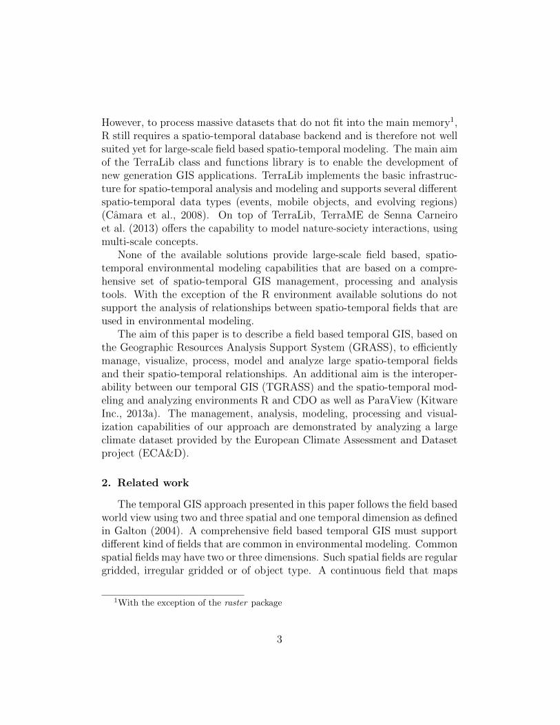
The temporal topology describes temporal relations between time stampsrepresented by interval time or time instances. Several algorithms in TGRASSneed to check the temporal topology of space time datasets for validity. Thecomputation of the temporal topology of a space time dataset is based ontemporal logic introduced in Allen (1983) shown in Figure 1. A valid tem-poral topology allows only the following temporal relationships: follows/pre-cedes and after/before.

Figure 1: Temporal relations between time intervals (Allen, 1983)

2.1.3. Temporal sampling

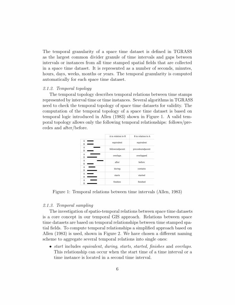
The investigation of spatio-temporal relations between space time datasetsis a core concept in our temporal GIS approach. Relations between spacetime datasets are based on temporal relationships between time stamped spa-tial fields. To compute temporal relationships a simplified approach based onAllen (1983) is used, shown in Figure 2. We have chosen a different namingscheme to aggregate several temporal relations into single ones:

• start includes equivalent, during, starts, started, finishes and overlaps.This relationship can occur when the start time of a time interval or atime instance is located in a second time interval.

6

• overlap includes overlaps and overlapped.

• contain includes contains, started and finished.

• during includes during, starts and finishes.

In TGRASS we denote the process to identify temporally related spatial fieldsof two space time datasets as temporal sampling. The sampling methods aredescribed in Figure 3.

Figure 2: Simplified temporal relationship scheme for space time datasetsampling.

A1 A2 A3 A4 A5

S1 S2 S3 S4 S5

Dataset with time instances

Dataset with time intervalsused for sampling

S1

S2

S3

S4

S5

start

A1

A2

A3,A4

A5

B1 B2 B3 B4 B5Dataset with time intervals

S1

S2

S3

S4

S5

start

B1

B2

B3

B5

B4

during contain overlap equal

B3

B1

B1,B2

B2

B5

B4

Sampling time instances Sampling time intervals

2001 2002 2003 2004 2005 2006 2007 2008 2009

Time in years

Figure 3: Methods of space time dataset sampling. Visualized are the tem-poral relations from time stamped spatial fields A and B to S. Hence A1starts in S1, B3 is during S3, B4 equals S4, B1 overlaps S1.

7

2.1.4. States, Events and Processes

Multiple concepts of states, events and processes have been developed.In our approach a single snapshot represents a specific state of a part of theworld at a discrete time instance or in a time interval. Langran (1992) statedthat changes between states are defined as events. An event transforms onestate into the next, hence change can not be represented using a snapshotapproach. The Event-Based Spatiotemporal Data Model (ESTDM) (Peuquetand Duan, 1995) uses time as an organizational basis to store event basedchanges. Sparse raster structures are used to represent the differences to abase raster layer that defines the state at the beginning of the time series.Worboys (1998) made the distinction that field based approaches allow thedefinition of processes and the object based approach allows the definitionof events. Yuan (2001) claims that processes are a sequence of dynamicallyrelated states and events are the occurrence of something significant such as aflood, a storm events or a wildfire. Events may consists of multiple processesand processes may be part of different events.

TGRASS supports the detection of events in spatio-temporal fields. Tem-porally related snapshots can be identified and differences between them canbe computed. TGRASS does not use a specific sparse data structure to storedifferences between spatial fields. The computational effort to detect differ-ences is much higher than in the ESTDM approach and the data storage isnot as efficient. However, TGRASS supports in contrast to the ESTDM ap-proach the computation of differences and the storage of 2D and 3D griddedspatial fields and fields of spatial objects. With the introduction of space timedatasets in TGRASS we are able to efficiently manage and analyze processesthat were defined by Yuan (2001).

2.2. GRASS GIS

The spatial GIS to integrate time must support spatial fields that areused in environmental modeling. In addition spatial querying, analysis andprocessing tools must be available. The design of the spatial GIS must pro-vide a well documented Application Programming Interface (API) to enablea strong3 integration of time. Reusing existing spatial analysis tools and algo-rithms in spatio-temporal work flows must be supported to avoid redundant

3Strong in the meaning that functionality of the temporal GIS framework can be inte-grated in the core functionality of the chosen GIS

8

implementations.We have chosen the Geographic Resources Analysis Support System GRASS

for time integration. GRASS is an Open Source Geographical InformationSystem that supports all needed spatial and integration specific requirements.Neteler et al. (2012) stated:

Due to the scientific background of many of its contributors, andits historical background, GRASS is well equipped for environ-mental modeling, and at the same time it retains the usefulnessfor a multi-purpose GIS environment.

In addition to the GRASS GIS website4 the text book by Neteler and Mi-tasova (2008) provides detailed information about this open source GIS.GRASS GIS has been utilized in many spatio-temporal environmental scien-tific applications (Mitasova et al., 1995, 2011, Neteler, 2005, 2010, Zorer et al.,2011). A comprehensive overview about GRASS GIS and its application inenvironmental modeling is available in Neteler et al. (2012).

3. The integration of time in GRASS GIS

3.1. Implementation

According to (Langran, 1992, page 5) the fundamental functions of atemporal GIS are:

• Inventory: Storing a complete description of the study area, and ac-count for changes in both the physical world and computer storage.

• Analysis: Explain, exploit, or forecast the components contained bythe process at work in a region.

• Update: Superseding outdated information with current information.

• Quality control: Evaluate whether new data are logically consistentwith previous versions and states.

• Scheduling: Identifying or anticipating threshold database states, whichtrigger predefined system responses.

4http://grass.osgeo.org

9

• Display: Generating a static or dynamic map, or a tabular summary,of temporal processes at work in region.

Except for scheduling, all the requirements of a temporal GIS specified abovewere implemented with a focus on inventory, analysis and quality. Besides ofthe environmental modeling requirements, design rules to integrate time inGRASS GIS were considered. An important integration aspect was to avoidthe break of existing functionality. To avoid redundancy existing modulesand libraries were reused for spatio-temporal field processing. Our imple-mentation follows the GRASS GIS design rule Create small and fast modulesfor a specific purpose and combine them to manage complex tasks.

A single spatial field is usually denoted as a layer in common GIS. How-ever, we will use the GRASS GIS specific notation raster map, 3D raster mapand vector map in this paper. Two and three dimensional regular griddedfields are referred as raster and 3D raster maps. Irregular gridded spatialfields and object fields are referred as vector maps.

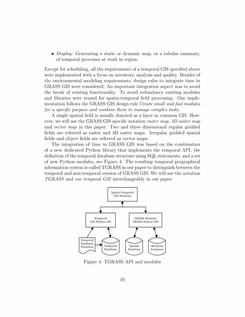
The integration of time in GRASS GIS was based on the combinationof a new dedicated Python library that implements the temporal API, thedefinition of the temporal database structure using SQL statements, and a setof new Python modules, see Figure 4. The resulting temporal geographicalinformation system is called TGRASS in our paper to distinguish between thetemporal and non-temporal version of GRASS GIS. We will use the notationTGRASS and our temporal GIS interchangeably in our paper.

Figure 4: TGRASS API and modules

10

To assure spatial database compatibility of TGRASS with existing GRASSdatabases, a dual storage concept was implemented. The spatial and at-tribute data storage concept of GRASS was not modified. All spatial datais stored in the GRASS spatial database using the existing GRASS specificstorage format. Vector attributes are stored in SQL databases. In additiona dedicated SQL database (temporal database) was introduced in TGRASSto store only temporal GIS related metadata.

3.1.1. Adding time stamps to maps

The first step to implement our temporal GIS was to integrate time stampsupport for raster, 3D raster and vector maps and therefore the design of thetemporal database. The existing time stamp mechanism for raster and 3Draster maps was reused and extended to support vector maps. In TGRASS,maps5 can be registered and unregistered in the temporal database. Whena map is registered, its unique id, the spatio-temporal extent and map typespecific metadata are stored in the temporal database. This concept leads toredundant storage, since this data is stored in the GRASS spatial databaseas well. The benefit of this storage scheme is that it allows complex SQLqueries using the spatio-temporal extent and metadata information for mapselection. It was not considered to choose a non-redundant storage scheme,since that would require a rewrite of the GRASS core library functionality.

3.1.2. Space Time Datasets

The introduction of three map type specific spatio-temporal data typesin TGRASS was the second integration step:

• Space Time Raster Datasets (STRDS) represent collections of timestamped raster maps

• Space Time 3D Raster Datasets (STR3DS) represent collections of timestamped 3D raster maps

• Space Time Vector Datasets (STVDS) represent collections of timestamped vector maps

Space time datasets (STDS) represent spatio-temporal fields in TGRASS.They are stored as table structures in the temporal database and can be

5Maps of type raster, 3D raster and vector.

11

created, updated and deleted. Raster, 3D raster and vector maps can beregistered in several different space time datasets at the same time. Thespatio-temporal extent as well as the granularity and the map type specificmetadata of space time datasets is automatically computed from registeredtime stamped maps. The correctness of time stamps and the temporal topo-logical validity is checked automatically. Cross referencing between timestamped maps and space time datasets was implemented to assure temporaldata integrity and consistency.

3.1.3. Space Time Voxel Cubes

The third step was the introduction of time as the third dimension inthe 3D raster GRASS C library to enable the support for space time voxelcubes. Space time voxel cubes support the same temporal types and timestamps as space time raster datasets. Space time raster datasets with validtemporal topology and interval time can be converted into space time voxelcubes. Every space time voxel cube can be converted into a space time rasterdataset. The conversion is performed without information loss. Space timevoxel cubes have equidistant sample resolutions for each axis (x, y, t). Theunit of the spatial axis depends on the projection of the GRASS location.The unit of the temporal axis depends on the chosen temporal unit that canbe of type years, months, days, hours, minutes or seconds. The axis specificspatial resolution is stored as double precision floating point values. In case ofabsolute time, the temporal resolution is stored as years, months or days withfractions of days representing hours, minutes and seconds relative to the dateJan. 1. 1900 00:00:00 UTC. This assures the correct temporal alignment ofspace time voxel cubes using the same temporal unit but different start orend times. All existing 3D raster modules can be used to process space timevoxel cubes. This includes modules for cross section computation, uni-variateand zonal statistical analysis, 3D mask creation and 3D point sampling.Map calculation that allows spatio-temporal algebraic operations describedin Jeremy et al. (2005) is supported as well. A limitation is that 3D mapcalculation is only allowed between space time cubes with the same temporalunit.

3.1.4. Spatio-temporal modules

In the last step temporal and spatio-temporal modules were implementedto provide spatio-temporal management, querying, analysis, processing, ex-port, import and conversion functionality. These modules were designed to

12

accept space time datasets as input for processing among maps of differenttype, numerical and textual parameter and files. Usually new space timedatasets or textual contents are created as output. The modular conceptof TGRASS allows nesting of temporal and spatial modules. Hence, theresult of a spatio-temporal query created with a temporal module can beused as input parameter for spatial processing modules. The naming con-cept of TGRASS modules follows the established module naming conventionof GRASS GIS:

• t.* prefix: Modules for temporal analysis and database management

• t.rast.* prefix: Modules processing space time raster datasets

• t.rast3d.* prefix Modules processing space time 3D raster datasets

• t.vect.* prefix: Modules processing space time vector datasets

An overview of implemented modules is given in Appendix A.

3.1.5. Visualization and data handling

TGRASS supports the direct visualization of raster time series. To cre-ate sophisticated animations including several space time raster and vectordatasets, the display modules6 can be utilized in conjunction with the tem-poral sampling module t.sample. Based on our temporal Python library newvisualization modules have been implemented by Kratochvilova (2013):

• g.gui.animate to visualize and animate multiple space time raster andvector datasets

• g.gui.timeline to visually analyze the temporal topology of multiplespace time raster and vector datasets

TGRASS was designed to handle and store high resolution, continentalscale data represented as maps and space time datasets. It was success-fully tested using different environmental datasets containing up to 150.000maps with hourly, daily, monthly and yearly temporal resolution. Space timedatasets that handle more than 20.000 maps were successfully used in spatio-temporal processing like aggregation and sampling. Limiting factors are thenumber and size of files and directories the used file system can manage andthe number and size of tables the temporal database can handle.

6d.mon, d.rast, d.vect, d.title, d.text, d.legend and many more

13

3.2. Interoperability

Interoperability of a temporal GIS with existing spatio-temporal model-ing, analysis and visualization applications multiplies its usefulness. Inter-operability avoids redundant implementation of the same functionality andallows the user to combine different applications to perform complex tasks asingle application is not capable of. Export interfaces for space time datasetsand statistical spatio-temporal data to the following open source applicationsare provided:

• R environment for statistical computing (R)

• Climate Data Operator (CDO)

• ParaView

The statistical analysis spatio-temporal modules of TGRASS support out-put formats that can be directly imported in R for further analysis. Withthe introduction of space time voxel cubes a new export module to createNetCDF files was implemented. This export module r3.out.netcdf supportsthe export of spatial volumes and space time voxel cubes as NetCDF files.Comprehensive projection information as well as data and axis descriptionsare provided in the NetCDF file, following the Climate and Forcast (CF)Conventions version 1.67. This assures seamless processing, analysis and vi-sualization of space time voxel cubes in R, CDO and ParaView. Additionally,the export of space time raster datasets as ParaView time series data usingthe legacy VTK (Kitware Inc., 2013b) format is provided.

4. Software availability

The source code of our implementation is licensed under the Gnu PublicLicense (GPL) version 2 and is part of GRASS GIS 7. It is available via thesoftware versioning and revision control system subversion8 starting fromGRASS GIS 7 revision 52369. The source code can be inspected using theGRASS GIS online source code browser9. Detailed compiling and installation

7http://cf-pcmdi.llnl.gov/documents/cf-conventions/1.6/

cf-conventions-multi.html8http://trac.osgeo.org/grass/wiki/DownloadSource#GRASS79http://trac.osgeo.org/grass/browser/grass/trunk

14

instructions as well as needed requirements are available at the GRASS GISweb site10. The author of TGRASS is Soren Gebbert.

5. Validation and verification

The functionality of the temporal GIS Python library was validated usingautomated Python tests that are directly integrated with the library sourcecode. Additionally, more than 100 tests to validate the temporal and spatio-temporal modules were implemented using shell scripts.

The seasonal and yearly mean temperatures from 1950 - 2011 of the tem-perate climate zone of the European Union and Turkey were analyzed, to ver-ify the inventory, analysis, modeling and display functionality of TGRASS aswell as the data exchange capabilities with R and ParaView. A detailed de-scription with code examples is available in Appendix B. The E-OBS datasetsof daily temperature and daily precipitation with a spatial resolution of 0.25degrees (Haylock et al., 2008) was used for this analysis. The daily mean tem-perature data was imported and registered in a new space time raster datasetwith 22644 maps using the modules r.in.gdal, t.create and t.register. The nextstep was the monthly, seasonal and yearly aggregation of the daily averagetemperature data with t.rast.aggregate. The module t.rast.extract was usedto extract specific space time raster datasets for each season. Then for eachseason specific STRDS the linear regression slope was computed from 1950- 2011 with t.rast.series. The resulting maps are visualized in Figure 5. Themodule t.rast.univar was used to compute the mean seasonal temperaturetime series of the temperate climate zone. The output of t.rast.univar wasimported into R to create the visualization shown in Figure 6a. Three vectorpoints were created using the coordinates of the three capital cities Berlin,London and Paris. The points were used to sample the seasonal mean tem-perature space time raster datasets using t.vect.observe.strds. The resultingdata were extracted with t.vect.db.select and visualized with R, see figures6b, 6c and 6d. The 5 year mean temperature of the yearly temperature spacetime raster dataset was computed with r3.mapcalc after the conversion of theSTRDS into a space time voxel cube with t.rast.to.rast3. The resulting spacetime voxel cube with a temporal extent from 1952 to 2008 and a granularityof one year was exported as netCDF file with r3.out.netcdf and visualized

10http://grass.osgeo.org/

15

(a) Linear regression slope of spring meantemperature

(b) Linear regression slope of summer meantemperature

(c) Linear regression slope of fall mean tem-perature

(d) Linear regression slope of winter meantemperature

Figure 5: The linear regression slope computed for all seasons from 1950 -2011. Red color indicates rising temperature, blue indicates falling temper-ature. Units are degree Celsius per year.

16

●●●●

●●

●

●●

●

●●●

●●

●

●●●●●●●●

●

●●

●●

●●●●

●

●●●

●

●●●●

●

●

●●

●

●●

●●

●●

●

●●

●●●●

●

1950 1960 1970 1980 1990 2000 2010

−5

05

1015

20

Years

Tem

pera

ture

in d

egre

e C

elsi

us

Seasonal mean temperature trend of the temperate European climate Zone from 1950 − 2010

● Summer temperature, linear regression slope 0.019Fall temperature, linear regression slope 0.006Spring temperature, linear regression slope 0.023Winter temperature, linear regression slope 0.019

(a) Seasonal temperature trend for Europe

●●

●●

●

●

●

●●

●

●●

●

●●

●

●●●●●●●

●

●

●●

●●

●●

●

●●

●●

●

●

●●●●

●

●

●●

●

●

●

●

●●

●

●

●●

●

●●

●

●

1950 1960 1970 1980 1990 2000 2010

−5

05

1015

2025

Years

Tem

pera

ture

in d

egre

e C

elsi

us

Seasonal mean temperature trend of Berlin from 1950 − 2010


(b) Seasonal temperature trend for Berlin

●

●

●

●

●

●

●

●●

●

●●

●●

●

●●

●

●

●●

●

●

●

●

●

●

●●

●●

●

●

●

●

●

●●●

●●

●●

●

●●

●

●

●

●●

●●

●

●●

●

●●●

●

1950 1960 1970 1980 1990 2000 2010

05

1015

20

Years

Tem

pera

ture

in d

egre

e C

elsi

us

Seasonal mean temperature trend of London from 1950 − 2010


(c) Seasonal temperature trend for London

●

●

●

●

●

●

●

●●

●

●●

●●

●

●

●●

●

●●

●

●

●

●

●

●

●●

●●

●

●

●

●

●

●

●●

●●

●

●

●

●●

●

●

●

●

●●●

●

●

●●

●●

●●

1950 1960 1970 1980 1990 2000 2010

05

1015

2025

Years

Tem

pera

ture

in d

egre

e C

elsi

us

Seasonal mean temperature trend of Paris from 1950 − 2010


(d) Seasonal temperature trend for Paris

Figure 6: Mean temperature trend for the temperate climate zone of theEuropean Union and the capitals Berlin, London and Paris.

17

with ParaView. Four screenshots of the ParaView time series visualizationare shown in Figure 7.

6. Discussion

This paper presents TGRASS, a temporal GIS for field based environ-mental modeling. We demonstrate that an existing spatial geographic infor-mation system can be modified into a field based temporal GIS. An extendedsnapshot approach allows the reuse of the spatial management, analysis, pro-cessing and visualization capabilities of GRASS for spatio-temporal tasks.

GRASS provides support for different spatial fields represented as raster,3D raster and vector maps. We integrated the time dimension in GRASS byimplementing time stamp support for all spatial fields. Spatio-temporal fieldsare represented in TGRASS as space time datasets. Space time datasets al-low the efficient handling, analysis and processing of massive data using sim-ple temporal GIS commands. Dedicated modules for temporal managementsimplify the handling of space time datasets and time stamped maps. Thedecision to use linear discrete time instances and intervals as time stamps forspatial fields allows a broad application in environmental modeling. Cyclictime can be emulated using scripts that loop over space time datasets. Dif-ferent branches from branching time can be represented by scenario specificspace time datasets. However, the linear discrete time approach leads tomanagement overhead for models that are based on cyclic or branching time.

Our approach allows the investigation of spatio-temporal relations be-tween space time datasets of different kind (raster, 3D raster and vector)using a combination of temporal sampling methods and spatial samplingmodules. The module t.sample was designed to describe the temporal rela-tionships between space time datasets. The textual output of this module canbe used as input for several spatial modules that perform spatial samplingfor example: r3.cross.rast, v.what.rast, v.what.rast3, v.what.vect, v.rast.stats.

Map calculations between space time datasets of type raster or 3D rasterare supported by dedicated modules using different temporal sampling meth-ods. The module r3.mapcalc can be used for sophisticated spatio-temporalmap calculations of space time voxel cubes. Neighborhood analysis as pro-vided for space time voxel cubes using r3.mapcalc are not supported for spacetime raster and 3D raster datasets. However, space time raster datasets withvalid temporal topology and interval time can be converted into space timevoxel cubes using the module t.rast.to.rast3.

18

(a) Five year mean temperature in 1960 (b) Five year mean temperature in 1975

(c) Five year mean temperature in 1990 (d) Five year mean temperature in 2005

Figure 7: Four screenshots showing the five year mean temperature of theEuropean Union and Turkey visualized with ParaView as key frame anima-tion from 1952 to 2008. Contour lines have been created for 9, 10 and 11degree Celsius.

19

Spatio-temporal queries are supported for all space time datasets usinga combination of SQL WHERE statements for temporal related selectionand the spatial and attribute querying capabilities of spatial modules. Inaddition, simple spatio-temporal and attribute specific queries are supportedas SQL WHERE statements, since the temporal and spatial extent as wellas map specific metadata is stored in the temporal SQL database.

TGRASS supports states, events and processes. States are an essentialpart of our temporal GIS approach. Events can be detected by combining thetemporal topology capabilities of TGRASS with its spatial overlay function-ality. Hence differences between temporally related time stamped maps canbe computed and stored, regardless of the type of the maps. However, ourapproach lacks efficiency in storage and computation in comparison to theESTDM approach. The representation of a process (Yuan, 2001) is availablein TGRASS using space time datasets.

In the context of field-based modelling, a remaining future challenge isto better visualize space time datasets, and to handle events and nested pro-cesses more efficiently. In the broader context of modelling spatio-temporalphenomena, challenges the integration of our field based modelling environ-ment with non-field based phenomena such as trajectories, lattice data, and(marked) point patterns (Stasch et al., 2014).

7. Conclusion

We implemented TGRASS, a temporal GIS for field based environmentalmodeling based on the open source geographical information system GRASS.The introduction of space time datasets that represent spatio-temporal fieldsin TGRASS, allows the efficient management and processing of massive envi-ronmental data and the analysis of relations between spatio-temporal fields.A comprehensive tool set for spatio-temporal management, analysis, pro-cessing and visualization is now available with the implementation of severaltemporal and spatio-temporal modules and the possibility to combine spa-tial modules with temporal modules. Our temporal GIS supports the importand export of the widely used spatio-temporal data format netCDF to assuredata interoperability to existing sophisticated spatio-temporal analysis andvisualization software CDO and ParaView. The structured textual outputof the analysis modules allows the direct processing and visualization withthe R statistical environment. The analysis of a massive climate dataset hasdemonstrated the environmental modeling capabilities of our approach.

20

Acknowledgements

We would like to thank Annette Freibauer and Rene Dechow for theirhelp and critical review of this work.

Allen, J. F., 1983. Maintaining knowledge about temporal intervals. Com-munications of the ACM 26 (11), 832–843.

Aquaveo LLC, 2013. Arc Hydro Groundwater.URL http://www.aquaveo.com/archydro-groundwater

Bettini, C., Dyreson, C. E., Evans, W. S., Snodgrass, R. T., 1998. A Glossaryof Time Granularity Concepts. Lecture Notes in Computer Science 1399.

Camara, G., Vinhas, L., Ferreira, K. R., De, G. R., Cartaxo, R., Souza, M.,Miguel, A., Monteiro, V., Carvalho, M. T. D., Casanova, M. A., De, U. M.,2008. Terralib: An open source gis library for large-scale environmental andsocio-economic applications.URL http://www.terralib.org/

Christakos, G., Bogaert, P., Serre, M. L., 2001. Temporal GIS: advancedfunctions for field-based applications. Springer.

Cova, T., Church, R., Goodchild, M., 2002. Extending geographical rep-resentation to include fields of spatial objects. International Journal ofGeographical Information Science 16, 509—532.

de Senna Carneiro, T. G., de Andrade, P. R., Cmara, G., Monteiro, A. M. V.,Pereira, R. R., 2013. An extensible toolbox for modeling naturesocietyinteractions. Environmental Modelling & Software 46 (0), 104 – 117.URL http://www.sciencedirect.com/science/article/pii/

S1364815213000534

Discovery Software Ltd., 2013. STEMgis: a Temporal Geographic Informa-tion System. 11 St. Mary’s Park, Paignton, Devon, TQ4 7DA, UnitedKingdom.URL http://www.discoverysoftware.co.uk/STEMgis.htm

Dyreson, C., Grandi, F., Kafer, W., Kline, N., Lorentzos, N., Mitsopoulos,Y., Montanari, A., Nonen, D., Peressi, E., Pernici, B., Roddick, J. F.,Sarda, N. L., Scalas, M. R., Segev, A., Snodgrass, R. T., Soo, M. D.,

21

Tansel, A., Tiberio, P., Wiederhold, G., Mar. 1994. A consensus glossaryof temporal database concepts. SIGMOD Rec. 23 (1), 52–64.

Forer, P., 1998. Geometric approaches to the nexus of time, space, and mi-croprocess: implementing a practical model for mundane socio-spatial sys-tems. In: Egenhofer MJ, Golledge RG (eds) Spatial and temporal rea-soning in Geographic Information Systems. Oxford University Press, NewYork/Oxford, pp. 171 – 190.

Frank, U., 1998. Different types of ”Time” in GIS. In: Egenhofer MJ,Golledge RG (eds) Spatial and temporal reasoning in Geographic Infor-mation Systems. Oxford University Press, New York/Oxford, pp. 40 – 62.

Galton, A., 2001. A Formal Theory of Objects and Fields. Spatial Informa-tion Theory. Foundations of Geographic Information Science : Interna-tional Conference, COSIT 2001 Morro Bay, CA, USA, September 19-23,2001. Proceedings, 458–473.

Galton, A., 2004. Fields and Objects in Space, Time, and Space-time. SpatialCognition & Computation 4 (1), 39–68.

Goodchild, M., Gopal, S., 1989. Modeling error in objects and fields. Accu-racy of Spatial Databases, 107–114.

Goodchild, M. F., May 1992. Geographical data modeling. Computers &Geosciences 18 (4), 401–408.

Hardisty, F., 2013. GeoViz: toolkit for geographic visualization and analysis.URL http://code.google.com/p/geoviz/

Haylock, M. R., Hofstra, N., Tank, A. M. G. K., Klok, E. J., Jones, P. D.,New, M., Oct. 2008. A European daily high-resolution gridded data setof surface temperature and precipitation for 1950 - 2006. Journal of Geo-physical Research 113 (D20).

Jeremy, M., Roland, V., Dana, T. C., 2005. Cubic map algebra functions forspatio-temporal analysis. Cartography and Geographic Information Sci-ence 32 (1), 17–32.

Kitware Inc., 2013a. ParaView: an open-source, multi-platform data analysisand visualization application.URL http://www.paraview.org/

22

Kitware Inc., 2013b. Visualization Toolkit (VTK): an open-source, freelyavailable software system for 3d computer graphics, image processing andvisualization.URL http://www.vtk.org/

Kratochvilova, A., 2013. Visualization of spatio-temporal data in grass gis.Master’s thesis, Faculty of Civil Engineering, Czech Technical Universityin Prague.URL http://geo.fsv.cvut.cz/proj/dp/2013/

anna-kratochvilova-dp-2013.pdf

Langran, G., Mar. 1992. Time in geographic information systems. Taylor &Francis.

Mitasova, H., Hardin, E., Starek, M., Harmon, R. S., Overton, M., 2011.Landscape dynamics from lidar data time series. In: Hengl, T., Evans,I. S., Wilson, J. P., Gould, M. (Eds.), Geomorphometry 2011. Redlands,CA, pp. 3–6.

Mitasova, H., Mitas, L., Brown, W., Gerdes, D., Kosinovsky, I., Baker, T.,Jul. 1995. Modelling spatially and temporally distributed phenomena: newmethods and tools for GRASS GIS. International Journal of GeographicalInformation Science 9 (4), 433–446.

Neteler, M., 2005. Time series processing of MODIS satellite data for land-scape epidemiological applications. International Journal of Geoinformat-ics. Special Issue on FOSS/GRASS 2004 & GIS-IDEAS 2004 1 (1), 133–138.

Neteler, M., Jan. 2010. Estimating Daily Land Surface Temperatures inMountainous Environments by Reconstructed MODIS LST Data. RemoteSensing 2 (1), 333–351.

Neteler, M., Bowman, M. H., Landa, M., Metz, M., 2012. GRASS GIS: Amulti-purpose open source GIS. Environmental Modelling & Software 31,124–130.

Neteler, M., Mitasova, H., Nov. 2008. Open Source GIS: A GRASS GISApproach, 3rd Edition. Springer, New York.URL http://www.grassbook.org/

23

O’Sullivan, D., Dec. 2005. Geographical information science: time changeseverything. Progress in Human Geography 29 (6), 749 –756.

Ott, T., Swiaczny, F., 2001. Time-integrative geographic information sys-tems: management and analysis of spatio-temporal data. Springer.

PCRaster team, 2012. PCRaster: a collection of tools and software librariesfor environmental modeling.URL http://pcraster.geo.uu.nl/

Pebesma, E., 2012. spacetime: Spatio-Temporal Data in R. Journal of Sta-tistical Software 51 (7).

Pelekis, N., Theodoulidis, B., Kopanakis, I., Theodoridis, Y., Jun. 2004. Lit-erature review of spatio-temporal database models. The Knowledge Engi-neering Review 19 (3), 235 – 274.

Peuquet, D., Duan, N., Jan. 1995. An event-based spatiotemporal data model(ESTDM) for temporal analysis of geographical data. International Journalof Geographical Information Science 9 (1), 7–24.

Peuquet, D. J., Hardisty, F., 2010. STempo: an interactive visualization andstatistical environment for discovery and analysis of space-time patterns.URL http://www.geovista.psu.edu/stempo/

R Development Core Team, 2012. R: A Language and Environment for Sta-tistical Computing. R Foundation for Statistical Computing, Vienna, Aus-tria, ISBN 3-900051-07-0.URL http://www.R-project.org

Schulzweida, U., 2013. Climate Data Operators: a large tool set for workingon climate and NWP model data.URL http://code.zmaw.de/projects/cdo

Stasch, C., Scheider, S., Pebesma, E., Kuhn, W., 2014. Meaningful spatialprediction and aggregation. Environmental Modelling & Software 51 (0),149 – 165.URL http://www.sciencedirect.com/science/article/pii/

S1364815213001977

24

Worboys, M. F., 1998. A generic model for spatio-bitemporal geographicinformation. In: Egenhofer MJ, Golledge RG (eds) Spatial and temporalreasoning in Geographic Information Systems. Oxford University Press,New York/Oxford, pp. 25 – 39.

Yuan, M., Apr. 2001. Representing Complex Geographic Phenomena in GIS.Cartography and Geographic Information Science, 83–96.

Yuan, M., 2009. Challenges and critical issues for temporal GIS researchand technologies. In: Hassan A. Karimi (eds) Handbook of Research onGeoinformatics. IGI Global, Hershey, pp. 144–153.

Zorer, R., Rocchini, D., Delucchi, L., Zottele, F., Meggio, F., Neteler, M.,Jul. 2011. Use of multi-annual MODIS land surface temperature data forthe characterization of the heat requirements for grapevine varieties. In:Analysis of Multi-temporal Remote Sensing Images (Multi-Temp), 20116th International Workshop on the. IEEE, pp. 225–228.

25

Appendix A. Temporal GRASS GIS Modules

Table A.1: Modules for temporal analysis and database management

Module Descriptiont.connect Sets or shows the temporal GIS database connection

information of the current mapsett.create Create the structure of a new space time dataset in the

temporal GIS databaset.info Lists information about space time datasets and maps

registered in the temporal GIS databaset.list Lists space time datasets and maps that are registered

in the temporal databaset.register Register raster, vector and 3D raster maps in the tempo-

ral GIS database or additionally in a space time datasett.remove Remove space time datasets from the temporal GIS

databaset.rename Renames a space time datasett.sample Sample input space time dataset(s) with a sample space

time dataset and print the resultt.support Modifies and update the metadata of a space time

datasett.topology List temporal relations of the maps in a space time

datasett.unregister Unregister raster, vector and 3D raster maps from the

temporal GIS database or a specific space time dataset

26

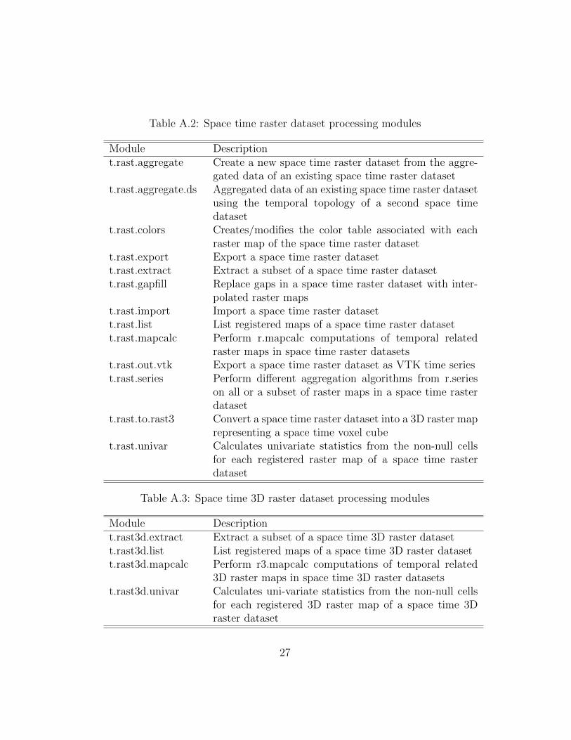
Table A.2: Space time raster dataset processing modules

Module Descriptiont.rast.aggregate Create a new space time raster dataset from the aggre-

gated data of an existing space time raster datasett.rast.aggregate.ds Aggregated data of an existing space time raster dataset

using the temporal topology of a second space timedataset

t.rast.colors Creates/modifies the color table associated with eachraster map of the space time raster dataset

t.rast.export Export a space time raster datasett.rast.extract Extract a subset of a space time raster datasett.rast.gapfill Replace gaps in a space time raster dataset with inter-

polated raster mapst.rast.import Import a space time raster datasett.rast.list List registered maps of a space time raster datasett.rast.mapcalc Perform r.mapcalc computations of temporal related

raster maps in space time raster datasetst.rast.out.vtk Export a space time raster dataset as VTK time seriest.rast.series Perform different aggregation algorithms from r.series

on all or a subset of raster maps in a space time rasterdataset

t.rast.to.rast3 Convert a space time raster dataset into a 3D raster maprepresenting a space time voxel cube

t.rast.univar Calculates univariate statistics from the non-null cellsfor each registered raster map of a space time rasterdataset

Table A.3: Space time 3D raster dataset processing modules

Module Descriptiont.rast3d.extract Extract a subset of a space time 3D raster datasett.rast3d.list List registered maps of a space time 3D raster datasett.rast3d.mapcalc Perform r3.mapcalc computations of temporal related

3D raster maps in space time 3D raster datasetst.rast3d.univar Calculates uni-variate statistics from the non-null cells

for each registered 3D raster map of a space time 3Draster dataset

27

Table A.4: Space time vector dataset processing modules

Module Descriptiont.vect.db.select Prints attributes of vector maps registered in a space

time vector datasett.vect.export Export a space time vector datasett.vect.extract Extract a subset of a space time vector datasett.vect.import Import a space time vector datasett.vect.list List registered maps of a space time vector datasett.vect.observe.strds Observe specific locations in a space time raster dataset

over a periode of time using vector pointst.vect.what.strds Sample a space time raster dataset at spatio-temporal

locations of a space time vector datasett.vect.univar Compute uni-variate statistics of a space time vector

dataset based on a single attribute row

Appendix B. Analyzing seasonal mean temperatures in the tem-perate climate zone of Europe

This is a detailed description of the mean temperature E-OBS datasetanalysis that was used to verify the capabilities of TGRASS. The followingworkflow was performed on a 64Bit AMD Linux system. GRASS in version7 was compiled and installed from the source code. All commands must beexecuted in the GRASS Unix command shell.

The E-OBS temperature and precipitation gridded datasets, provided bythe ECA&D as netCDF files, has a daily temporal resolution and a spatialresolution of 0.25 degrees. The dataset was download as several compressednetCDF files from the ECA&D website11. Each netCDF file was importedinto GRASS GIS using the module r.in.gdal with the specification of theband number offset to assure chronological numbering of the imported rastermaps. The flag −o indicates that the projection check should be skipped toallow the import. The reason for this is that the ECAD netCDF files do notinclude projection informations.

1 r . in . gdal −o input=tg 0 .25 deg reg 1950 −1964 v5 . 0 . nc \2 output=temperature mean o f f s e t=03

11http://eca.knmi.nl/download/ensembles/data/Grid_0.25deg_reg/

28

4 r . in . gdal −o input=tg 0 .25 deg reg 1965 −1979 v5 . 0 . nc \5 output=temperature mean o f f s e t =547967 r . in . gdal −o input=tg 0 .25 deg reg 1980 −1994 v5 . 0 . nc \8 output=temperature mean o f f s e t =109579

10 r . in . gdal −o input=tg 0 .25 deg reg 1995 −2011 v5 . 0 . nc \11 output=temperature mean o f f s e t =16436

A space time raster dataset named temperature mean 1950 2011 daily wascreated to simplify the handling of more than 22000 raster maps:

1 t . create type=strds output=temperature mean 1950 2011 da i ly \2 temporal=abso lu t e \3 t i t l e=”European mean temperature 1950−2011” \4 description=”The European da i l y mean temperature from 1950 − 2011”

A small Python script was implemented that created the input text file forthe module t.register to support the registration of all imported raster mapsin the space time raster dataset temperature mean 1950 2011 daily. To gen-erate the interval time stamps the start date was set to the first of January1950 using a time increment of one day:

1 cat > ECAD cl imate data t imeser i e s 1950 2011 . py << EOF2 f i l e = open( ”map l i s t . txt ” , ”w” )3 for i in range (22461) :4 f i l e .write ( ” temperature mean.% i \n” % ( i + 1) )5 f i l e . c l o s e ( )6 EOF78 python ECAD cl imate data t imeser i e s 1950 2011 . py9

10 t . register − i type=rast input=temperature mean 1950 2011 da i ly \11 f i l e=map l i s t . txt start=1950−01−01 increment=”1 day”

The daily data was aggregated with the module t.rast.aggregate to monthly,seasonal and yearly granularity. Using the module g.region the correct regionand resolution for temporal aggregation was set. Spatial aggregation was notrequired in this case.

1 g . region −p rast=temperature mean . 123 t . rast . aggregate input=temperature mean 1950 2011 da i ly \4 method=average \5 output=temperature mean 1950 2011 monthly \6 base=temperature mean monthly \7 granularity=”1 month”89 t . rast . aggregate input=temperature mean 1950 2011 monthly \

10 method=average \11 output=temperature mean 1950 2011 seasona l \12 base=temperature mean seasonal \13 granularity=”3 months”\

29

14 where=” s t a r t t ime >= ’1950−03−01 ’ and s t a r t t ime < ’2011−02−01 ’”1516 t . rast . aggregate input=temperature mean 1950 2011 monthly \17 method=average \18 output=temperature mean 1950 2011 year ly \19 base=temperature mean year ly \20 granularity=”1 year ” \21 where=” s t a r t t ime < ’2011−01−01 ’”

The temperature raster maps of spring, summer, fall and winter were ex-tracted separately using SQL WHERE statements. This results in new spacetime raster datasets. Additionally the unit of the temperature was convertedfrom 0.01 degree Celsius into 1 degree Celsius using a raster map calcula-tion expression. The following command was repeated for each season usingdifferent monthly offsets and output naming:

1 t . rast . extract input=temperature mean 1950 2011 seasona l \2 output=temperature mean 1950 2011 spr ing \3 where=” s t a r t t ime = datet ime ( s t a r t t ime , ’ s t a r t o f year ’ , ’2 month ’ ) ” \4 expression=” temperature mean 1950 2011 seasona l / 100 .0 ” \5 base=temp mean spring

A mask was applied to analyze the seasonal temperature for the temperateclimate zone. The mask was based on the extraction of the thermal climatezone using the GRASS map calculator r.mapcalc and the thermal climatezone map provided by Environmental conditions of Food Insecurity, Povertyand Environment Global GIS Database (FGGD)12. Figure B.8 shows thesimplified climate zones map that was used. The temperature trend of spring,summer, fall and winter was computed with t.rast.series using the optionslope to compute the linear regression slope for each season. This sloperepresents the average temperature change per year in degree Celsius. Thefollowing command combination was repeated for each season:

1 t . rast . series input=temperature mean 1950 2011 spr ing \2 output=temperature mean 1950 2011 spr ing s lope \3 method=s lope

Additionally the color for each map was set to the predefined GRASS colortable differences by taking the temperature range of all maps into account.

1 r . colors map=tempera tu re mean 1950 2011 fa l l s l ope ,t emperature mean 1950 2011 spr ing s lope ,temperature mean 1950 2011 summer slope ,t emperature mean 1950 2011 winte r s lope \

2 color=d i f f e r e n c e

12http://www.fao.org/geonetwork/srv/en/metadata.show?id=14056

30

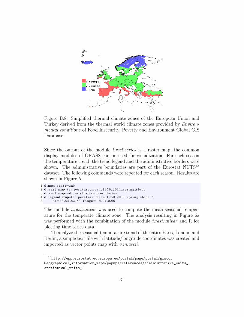
Figure B.8: Simplified thermal climate zones of the European Union andTurkey derived from the thermal world climate zones provided by Environ-mental conditions of Food Insecurity, Poverty and Environment Global GISDatabase.

Since the output of the module t.rast.series is a raster map, the commondisplay modules of GRASS can be used for visualization. For each seasonthe temperature trend, the trend legend and the administrative borders wereshown. The administrative boundaries are part of the Eurostat NUTS13

dataset. The following commands were repeated for each season. Results areshown in Figure 5.

1 d .mon start=wx02 d . rast map=temperature mean 1950 2011 spr ing s lope3 d . vect map=admin i s t r a t i v e bounda r i e s4 d . legend map=temperature mean 1950 2011 spr ing s lope \5 at =55 ,95 ,83 ,85 range=−0.04 ,0.06

The module t.rast.univar was used to compute the mean seasonal temper-ature for the temperate climate zone. The analysis resulting in Figure 6awas performed with the combination of the module t.rast.univar and R forplotting time series data.

To analyze the seasonal temperature trend of the cities Paris, London andBerlin, a simple text file with latitude/longitude coordinates was created andimported as vector points map with v.in.ascii.

13http://epp.eurostat.ec.europa.eu/portal/page/portal/gisco_

Geographical_information_maps/popups/references/administrative_units_

statistical_units_1

31

1 cat > c ap i t a l c o o r d s . txt << EOF2 Par i s |48 . 856667 |2 . 3516673 London |51 .50939 | −0 .118324 Ber l i n |52 . 518611 |13 . 4080565 EOF67 v . in . asc i i input=cap i t a l c o o r d s . txt output=obse rva t i on s \8 x=3 y=2 columns=” c ap i t a l TEXT, y DOUBLE, x DOUBLE”

The imported vector points observations were used to sample the spring,summer, fall and winter mean temperature using the module t.vect.observer.strds.New space time vector datasets were created to store for each time stampedraster map the point sampled values in time stamped attribute tables. Themodule t.vect.db.select was used to extract the temperature history for eachseason and city. The following command was used to create the observationsfor Paris in spring:

1 t . vect . observe . strds input=obse rva t i on s \2 output=sp r i n g ob s e r v a t i on s \3 vector=spr i ng ob s e rva t i on s 1950 2011 \4 strds=temperature mean 1950 2011 spr ing \5 column=temperature67 t . vect .db . select input=sp r i n g ob s e r v a t i on s where=” cat = 1” \8 column=temperature

The output of t.vect.db.select for each season and capital was imported intothe R statistical environment to create Figure 6b, 6c and 6d. This is ashortened version of the resulting output of t.vect.db.select :

1 s t a r t t ime | end time | temperature2 1950−03−01 00:00:00 |1950−06−01 00 : 00 : 00 |11 . 17257347673 1951−03−01 00:00:00 |1951−06−01 00 : 00 : 00 |9 . 71682437284 1952−03−01 00:00:00 |1952−06−01 00 : 00 : 00 |12 . 47415412195 . . .6 2008−03−01 00:00:00 |2008−06−01 00 : 00 : 00 |12 . 20553405027 2009−03−01 00:00:00 |2009−06−01 00 : 00 : 00 |12 . 58186738358 2010−03−01 00:00:00 |2010−06−01 00 : 00 : 00 |11 . 5653046595

The yearly aggregated mean temperature space time dataset was convertedinto a space time voxel cube to perform spatio-temporal map calculations.The goal was to compute the 5 year mean temperature for each voxel andto analyze it visually in ParaView for the European Union and Turkey.The first steps was to adjust the MASK and region settings with r.maskand g.region followed by the transformation using the module t.rast.to.rast3.Then the space time voxel cube map calculation was performed with themodule r3.mapcalc. The temporal unit and the time stamp must be explic-itly set with r3.support and t.register. Finally the resulting space time voxel

32

cube was exported as netCDF file and visualized with ParaView, see Figure7. The commands were executed in the following order:

1 r .mask the rma l c l imate zone s eu rope23 g . region −p3 rast=temperature mean . 145 t . rast . to . rast3 input=temperature mean 1950 2011 year ly \6 output=vol 1y mean78 g . region −p3 rast3=vol 1y mean9

10 r3 .mapcalc expression=”vol 5y mean = ( vol 1y mean [0 ,0 , −2 ] + \11 vol 1y mean [0 ,0 , −1 ] + \12 vol 1y mean [ 0 , 0 , 0 ] + \13 vol 1y mean [ 0 , 0 , 1 ] + \14 vol 1y mean [ 0 , 0 , 2 ] ) /500 .0 ”1516 t . register type=rast3 map=vol 5y mean start=”1950−01−01” end=”2011−01−01”17 r3 . support map=vol 5y mean vunit=” years ”1819 r3 . out . netcdf input=vol 5y mean output=vol 5y mean . nc null=−1000

33

a temporal gis for eld based environmental modeling

Documents