A Tutorial on Calculating and Interpreting Regression Coefficients in Health Behavior Research

Michael L. Stellefson, Bruce W. Hanik, Beth H. Chaney, and J. Don Chaney

Abstract

Regression analyses are frequently employed by health educators who conduct empirical research examining a variety of health behaviors. Within regression, there are a variety of coefficients produced, which are not always easily understood andlor articulated by health education researchers. It is important to not only understand what these coefficients are, but also understand what each represents and how each is interpreted. By correctly interpreting regression coefficients (pearson r, Pearson r', Mnltiple R', a, b, B, rs' r's' partial correlation and semi-partial correlation), the informed health behavior researcher can better understand the dynamics ofhis/her data. The purpose of this manuscript is to describe and explain some of the coefficients produced in regression analysis. Specifically, the manuscript will describe (a) why and when each regression coefficient is important, (b) how each coefficient can be calculated and explained, and (c) the uniqueness between and among specific coefficients. Adata set originally used by Holzinger and Swineford (1939) will be referenced throughout the manuscript to tangibly illustrate how coefficients should be calculated and interpreted in both simple and multiple regression analyses.

Regression analyses are frequently employed within empirical studies examining health behavior to determine correlations between variables of interest. Simple regression analyses can be used to predict or explain a continuously scaled dependent variable by using one continuously scaled independent variable. Multiple regression analyses can be used to investigate relationships between a single,

• Michael L. Stellefson, MS, Doctoral Candidate; Division of Health Education, Texas A&M University, MS 4243, College Station, TX 77843; Telephone: 979-458-0097; Fax: 979-862-2672; E-mail: mstell@hlkn.tamu.edu; Chapter: Alpha Pi

Bruce W. Hanik, MS, Doctoral Student; Division of Health Education, TexasA&M University, College Station TX, 77843; Chapter: Alpha Pi

Beth H. Chaney, PhD, CHES; Assistant Professor; Deparbnent of Health Education and Promotion, East Carolina University, 3205 Carol (l Belk Building, Greenville, NC, 27858; Chapter: Beta Theta

J. Don Chaney, PhD, CHES; Assistant Professor; Department of Health Education and Promotion, East Carolina University, 2302 Carol (l Belk Building, Greenville, NC 27858; Chapter: Beta Theta

• Corresponding author

continuous outcome variable and two or more continuous, predictor variables (Thompson, 2006). Within both types of regression, there are a variety of coefficients produced, which are not always easily understood and articulated by health education researchers. The purpose of this manuscript is to describe and explain a variety of regression coefficients used in regression analysis. Specifically, the manuscript will describe (a) why and when each regression coefficient is important, (b) how each coefficient can be calculated and explained, and (c) the uniqueness between and among specific coefficients. A data set originally used by Holzinger and Swineford (1939) will be utilized to demonstrate how to conduct and interpret both simple and multiple regression analyses. This data set reflects scores on 24 psychological tests administered to junior high school students to assess various acuities. It has been used by researchers to explain various analytic techuiques used throughout the history of statistics (Hetzel, 1996).

Pearllonr

Continuously scaled variables are variables which are measured on a scale of equal units. These are the types of variables that can be examined using regression analytic techniques. When two variables are measured on a continuous scale, we can compute the Pearson pToduct­moment correlation coefficient (r) between the two variables, computed as:

where COY xy is a description of bivariate relationship called the covariance and SDx and SDy are the standard deviations of both the independent (X) and dependent (Y) variables (Thompson, 2006). The covariance is used primarily as an intermediate calculation in obtaiuing the Pearson product moment correlation, because it does not have a defmitive range of possible values (Thompson, 2004). Pearson r addresses the question, "In an ordinary least squares distribution, how well does the line of best possible fit (regression line) capture the data points in a scattergram?" When Pearson r is positive, the relationship between two variables is positive. This means either (a) as scores on one variable become larger, scores on the other variable (on the average) tend to also be larger, or (b) as scores on one variable become smaller, scores on the other variable (on the average) tend to also become smaller. When Pearson r is negative, the relationship between two variables is negative .

12 The Health Educator Spring 2008, Vol. 40, No. 1

This means either (a) as scores on one variable become larger, scores on the other variable (on the average) tend to become smaller, or (b) as scores on one variable become smaller, scores on other variable (on the average) tend to become larger. The Pearson r is a descriptive statistic, quantifying the amount of linear relationship between two continuous variables. Pearson r statistics themselves, however, are ordinally scaled as regards to the variance common to two variables (Thompson, 2006); therefore, you cannot quantify the relationship between two distinct Pearson r values unless each is squared.

Pearson r' (also known as the coefficient of determination or the common variance proportion), unlike Pearson r, reflects the percentage of variance common to two variables (Thompson, 2006). This statistic is not ordinally scaled; rather, it is continuously scaled and thus a comparable statistic. It tells us that with knowledge of the scores on one predictive or explanatory, independent variable, we can explain or predict a given percentage, on the average, of the variability or Sum of Squares (SOS) of a dependent variable. One minus the Pearson r' yields the coefficient of alienation which describes the proportion of variance in the dependent variable that we cannot predict with knowledge of an independent variable (Thompson, 2006).

The SOSIlXPLAlNED' or the proportion of the SOS of the dependent variable that is linearly explained by the independent variable, divided by the SOSTOTAL' the total amount of explained and unexplained (i.e. not explained by the independent variable) variability in the dependent variable (y), tells us the proportion of the variability of individual differences that we can explain with an independent variable (X):

r' YX = SOSEXPLAINED I SOSlOTAL

In the case of two or more independent variables, the Pearson r' computation above becomes referred to as multiple R', to account for the multiple independent variables (XI, X2) having the opportunity to explain or predict the variance in the dependent variable (Y):

R' YXI.xz •... = SOSEXPLAINED I SOSrour.

Pearson r' and multiple R' measure the strength of the relationship between the independent variable(s) and dependent variable. Pearson r' (and multiple R') values have also been explained as indices which quantify the degree to which predicted scores match up with actoal scores (Huck, 2004).

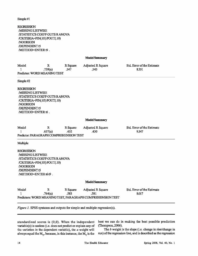
Figure I provides three SPSS (SPSS, Inc., 2006) syntaxes and outputs reflecting two simple (Simple #1 and Simple #2) and one multiple regression analysis using scores on variables t5 (paragraph Comprehension Test), t6 (General Information Verbal Test), and t9 (Word Meaning Test).

In the Simple #1 regression analysis, we are calculating the Pearson r' correlation between scores on the Word Meaning Test (entered as the independent variable) and General Information Verbal Test scores (entered as the dependent variable). Notice that the correlation between the two variables is r' = .547. In the Simple #2 regression analysis, we are calculating the Pearson r' correlation between scores on the Paragraph Comprehension Test scores (entered as the independent variable) and General Information Verbal Test scores (entered as the dependent variable). Notice that the correlation between the two variables is a bit srnaller, as r' = .432. In the Multiple regression analysis, we are calculating the multiple R' correlation to see the effect of Word Meaning Test scores (independent variable) and Paragraph Comprehension Test scores (indepedendent variable) on predicting General Information Verbal Test Scores (dependent variable). Notice that the multiple R' (.583) entering both predictors simultaneously is slightly larger than the r' (.547) between Word Meaning Test scores and General Information Verbal Test scores.

The Regression Equation

Regression analysis employs two types of weights: an additive constant, a, applied to every individual participant, and a multiplicative constant, b, applied to the entire predictor variable for each individual participant (Thompson, 2006). The weighting system takes the form of a regression equation that serves as the set of weights generated in a given analysis:

The a weight is the point where the regression line (i. e. line of best fit) crosses the y-axis when x equals O. This point is also called the y-intercept. To compute the a weight, one must determine an individual's predicted dependent variable score (Y) [see Note below]and their corresponding independent variable (X) score. The regression line always pivots on the mean of X (M,J and the mean of Y (My); therefore, the M" is itself a Y score corresponding to ~, given that this predicted dependent variable score (My) is always perfectly predicted to correspond with~. With this knowledge, the M" score can be input as the Y score in the regression equation.

When working with standardized scores (i. e. scores which have been standardized by removing or dividing by the standard deviation (SD) units of both the independent and dependent variables, the a weight will always be equal to zero, because the regression line always pivots on the Cartesian Coordinate ~, M,,), which when dealing with

Note: The statistical symbol that is to be a Latin capital letter Y with circumflex (character map:

U+O 176) is represented as Yin this article.

Spring 2008, Vol. 40, No.1 The Health Educator \3

Simple #1

REGRESSION !MISSING LISTWISE /STATISTICS COEFF OUTS RANOVA /CRITERlA~PIN(.05)POUT(.10)

INOORIGIN IDEPENDENTt5 IMETHOD=ENTER t9 .

Model R R Square I .739(a) .547

Predictor: WORD MEANING TEST

Simple #2

REGRESSION !MISSING LISTWISE /STATISTICS COEFF OUTS RANOVA /CRITERlA~PIN(.05)POUT(.10)

INOORIGIN IDEPENDENTt5 IMETHOD=ENTER t6 .

Model Summary

Adjusted R Square .545

Model Summary

Model R R Square Adjusted R Square I .657(a) .432 .430

Predictor: PARAGRAPH COMPREHENSION TEST

Multiple

REGRESSION !MISSING LISTWISE /STATISTICS COEFF OUTS RANOVA /CRlTERlA~PIN(.05)POUT(.10)

INOORIGIN IDEPENDENTt5 IMETHOD=ENTERt6t9 .

Mode\Summary

Model R R Square Adjusted R Square I .764(a) .583 .581

Predictors: WORD MEANING TEST, PARAGRAPH COMPREHENSIONTEST

Figure 1. SPSS syntaxes and outputs for simple and multiple regression(s).

Std. Error of the Estimate 8351

Std. Error of the Estimate 9347

Std. Error of the Estimate 8.017

standardized scores is (0,0). When the independent variable(s) is useless (i.e. does not predict or explain any of the variation in the dependent variable), the a weight will always equal the My, because, in this instance, the My is the

best we can do in making the best possible prediction (Thompson, 2006).

14

The b weight is the slope (Le. change in rise/change in run) of the regression line, and is described as the regression

The Health Educator Spring 2008, Vol. 40, No. 1

weight. The value of b signifies how many predicted units change (either up or down) in the dependent variable there will be for anyone unit increase in the independent variable. In a best case scenario, where the independent variable(s) perfectly predicts the outcome variable, the b weight perfectly matches the dispersions of the Y, (individual's actual score) and y. (individual's predicted score). When the predictor variable(s) is useless (i. e. does not predict or explain any of the variation in the outcome variable), the b weight will equal o to "kill" the useless independent variable and remove its influence from the regression equation (Thompson, 2006). If the metrics of the variables of interest have been standardized, the regression weight is expressed as beta (B). A positive B (or b) means that the slope of the regression line is positive, tilting from lower left to upper right, whereas a negative B ( or b) indicates that the slope of the regression in negative, tilting from upper left to lower right (Huck, 2004). Thus, the sign of b or B indicates the kind of correlation between the variables.

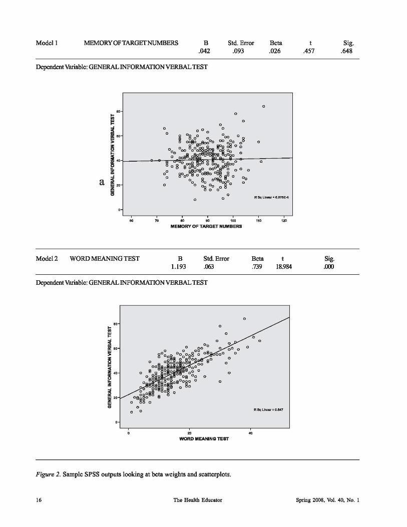
Consider the SPSS outputs and scatterplots contained in Figure 2. These were developed analyzing the Holtzinger and Swineford (1939) data set discussed earlier. Notice the non-statistically significant results (P = .648) at for the B weight (.042) describing the correlation between the Memory of Target Numbers test scores and the General Information Verbal test scores (Modell). Also, notice the flat regression line of best fit, indicating that the relationship between these two variables is neither positive nor negative (i. e., the relationship is non-existent). Conversely, notice the statistically significant (P = .001) B weight (.739) describing the positive relationship between the Word Meaning Test scores (utilized earlier) and the General Information Verbal test scores (Model 2). This relationship is evidenced by the line of best fit tilting from lower left to upper right.

The a and b (or B) weights are constants, in that they do not vary from individual score to individual score. Their function in the regression equation is primarily two fold. First, the b or B attempts to make the spreadoutness of the Y scores (predicted dependent variable scores) and Y scores (actual dependent variable scores) the same, which only happens when a predictor variable perfectly predicts a dependent variable. Second, the a weight seeks to make My=~ which it always accomplishes perfectly. Essentially, the multiplicative weight (b, Jl) begins the process by affecting the dispersion (SOSyand central tendency (My) of Y, and then the a weight is turned loose to make My = My.

Interpreting Regression Coefficients with Co"elated Predictors

When independent variables have nonzero Bs which do not equal the independent variable's respective Pearson r correlation with the dependent variable (y), the independent variables are said to be collinearwith one another. Collinearity refers to the extent which the independent variables have nonzero correlations with each other (Thompson, 2006). If

two or more independent variables are entered in a multiple regression and those variables are correlated with each other to a high degree and correlated with the dependent variable, then the B weights for the independent variables are arbitrarily allocated predictive/explanatory credit among the correlated independent variables. The independent variables with higher Bs are arbitrarily allocated credit for both uniquely and commonly explained area of the dependent variable. This allocation of predictive/explanatory credit given to each independent variable can happen only one time, since more than one independent variable can not be given predictive/ explanatory credit for the commonly explained area of the dependent variable (Y). Thus, one must determine what is uniquely explained by each independent variable and how predictive/explanatory credit is allocated among the independent variables for the area that is commonly explained. The formulas for the iis of two correlated predictnrs adjudicates the arbitrary allocation of shared credit (Thompson, 2006):

B, = ryxl-[(rYX2)( rXIX2)] / [1- r' XIX2]

B, =rYX2-[(rYXI)(rxI~] / [1- r'XIX2]

To mentally conceptualize how these formulas allocate credit between two independent variables operationalized in a type ill SOS situation, think of horses feeding in a trough. Think of the feed in the trough as the SOSy (SOS of the dependent variable) and each horse representing a unique independent variable, thus each possessing a unique SOSx (assuming the horses are of unequal sizes-i.e. unequal SOSs). The rYXI and rYX2 can be thought of as the amount of feed that each horse can eat from the trough. The rX1X2 is equivalent to the amount offeed that both horses commonly (yet individually) ate from the trough. The amount of feed that each horse ate from the trough may overlap among both horses, so it may be hard to distingnish which horse ate which proportion of the feed (given that the feed does not stay in a fixed position within the trough). However, as the farm handler, you may be asked to arbitrarily distingnish which horse ate which proportion of the feed. If you were able to view the amount of newly eaten feed present in each horse's stomach, then you would be able to see which horse ate more individually (describing both rYXI and r

YX2) and

thus give unique credit to each horse. You can not see this, however, so you must arbitrarily give credit to one (and only one) horse for eating a commonly eaten proportion of the feed (represented within ryxlX2),

The structure coefficient (r,) of a predictor variable is the correlation between the independent variable and Y (Thompson & Borrello, 1985). Recall that the collinearity of measured independent variables affects the is of these variables; however, collinearity does not effect rs computations. Thus, rss are incredibly useful for interpreting regression results (Thompson, 2006). Unless a researcher is (a) researching a specific set of independent variables which

Spring 2008, Vol. 40, No.1 The Health Educator 15

Modell MEMORYOFTARGETNUMBERS B .042

Dependent Variable: GENERAL INFORMATION VERBAL TEST

" m L o

o W > Z

~

Ii" 0 ~

;!; ....

a ill W20 o Z W

"

o o

Std. Error .093

o

o

o 0 CXl 0000 8

gg 0 g 00 0

00 o

o

o

o

o

Beta .026

o o RSq L~ -1I.waE-.4

eo 70

Model2 WORD MEANING TEST

eo 90 100

MEMORY OF TARGET NUMBERS

B 1.193

Std. Error .063

Dependent Variable: GENERAL INFORMATION VERBAL TEST

1-.. W 1-

~ !:! z

i 0 ~ ;!;

~ W Z W

" 0

0 0

0 20

WORD MEANING TEST

Figure 2. Sample SPSS outputs looking at beta weights and scatterplots.

16 The Health Educator

o

o

110

Beta .739

o

120

t

18.984

RSq~·O.547

..

t

.457

Sig. .000

Sig. .648

Spring 2008, Vol. 40, No. 1

are not even remotely affected by other independent variables or (b) researching independent variables which are perfectly uncorrelated, then rss should always be interpreted along with Jl weights (Courville & Thompson, 2001). Pedhazur (1982) objected to this necessity and noted that rss are simply correlations of independent variables with dependent variables divided by multiple R. This interpretation is mathematically valid, but neglects the idea that the focus of regression analysis is to understand the makeup of Y (the proportion of Y that is explained by the independent variables), not mathematically divide Pearson product moment correlations by multiple R.

Calculating and Interpreting Structure Coefficients (r ss) Using SPSS

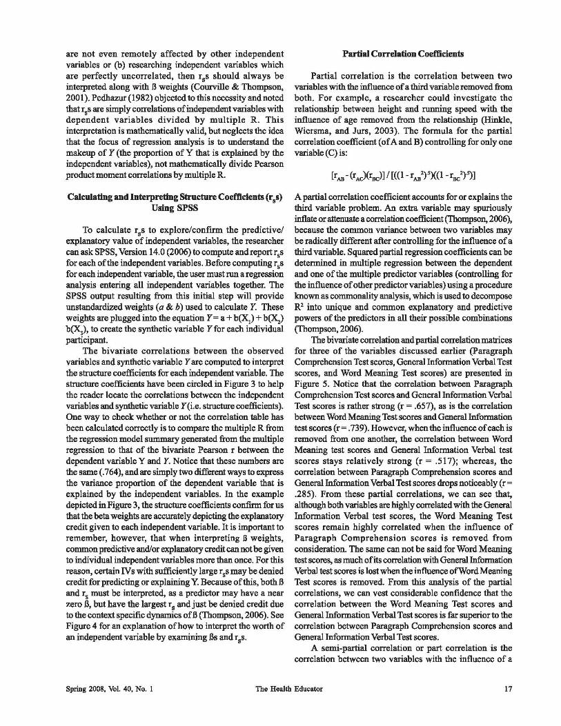
To calculate rss to explore/confrrm the predictive/ explanatory value of independent variables, the researcher can ask SPSS, Version 14.0 (2006) to compute and report rss for each of the independent variables. Before computing rss for each independent variable, the user must run a regression analysis entering all independent variables together. The SPSS output resulting from this initial step will provide unstandardized weights (a & b) used to calculate Y. These weights are plugged into the equation Y ~ a + b(X,) + b(X,) b(X,), to create the synthetic variable Y for each individual participant.

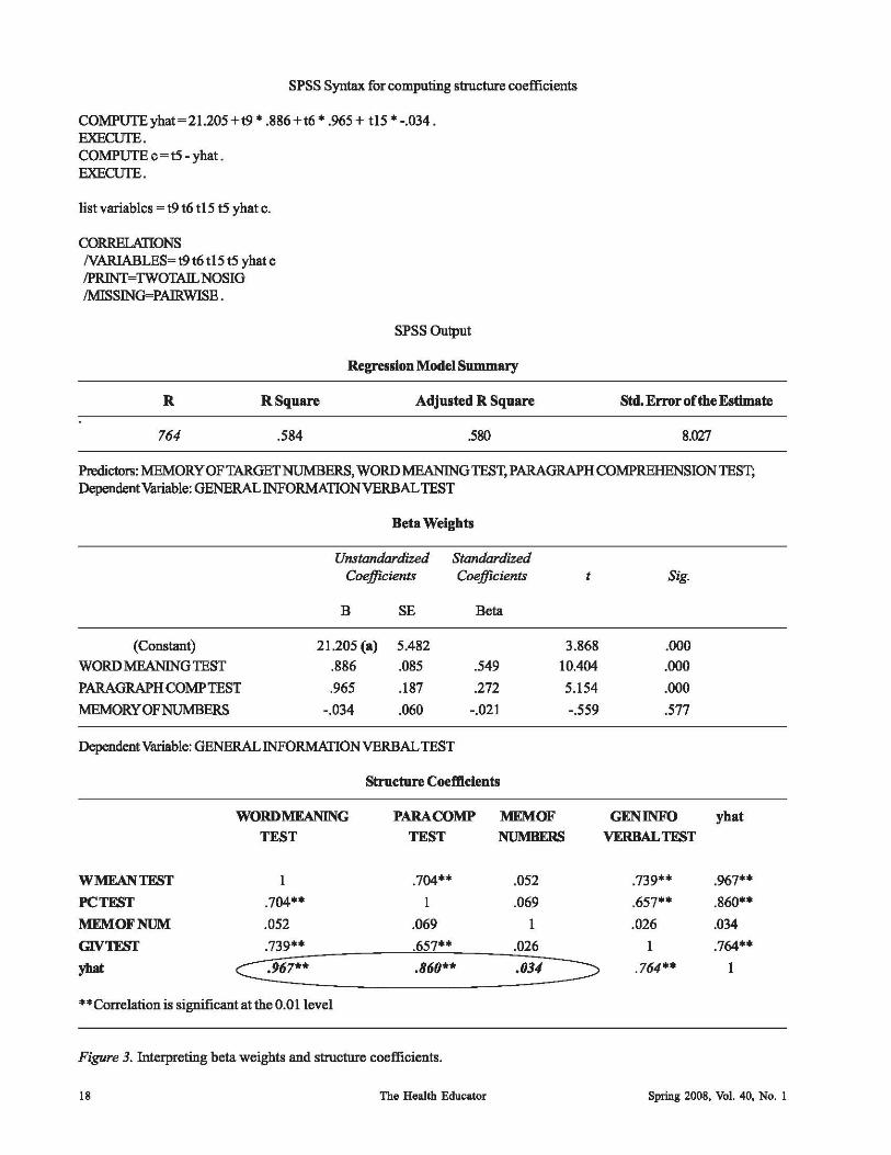
The bivariate correlations between the observed variables and synthetic variable Yare computed to interpret the structure coefficients for each independent variable. The structure coefficients have been circled in Figure 3 to help the reader locate the correlations between the independent variables and synthetic variable Y (i.e. structure coefficients). One way to check whether or not the correlation table has been calculated correctly is to compare the multiple R from the regression model summary generated from the multiple regression to that of the bivariate Pearson r between the dependent variable Y and Y. Notice that these numbers are the same (.764), and are simply two different ways to express the variance proportion of the dependent variable that is explained by the independent variables. In the example depicted in Figure 3, the structure coefficients confumforus that the beta weights are accurately depicting the explanatory credit given to each independent variable. It is important to remember, however, that when interpreting B weights, common predictive and/or explanatory credit can not be given to individual independent variables more than once. For this reason, certain N s with sufficiently large rss may be denied credit for predicting or explaining Y. Because of this, both Jl and rs must be interpreted, as a predictor may have a near zero Jl, but have the largest rs and just be denied credit due to the context specific dynamics of Jl (Thompson, 2006). See Figure 4 for an explanation of how to interpret the worth of an independent variable by examining Jls and rss.

Partial Correlation Coefficients

Partial correlation is the correlation between two variables with the influence of a third variable removed from both. For example, a researcher could investigate the relationship between height and running speed with the influence of age removed from the relationship (Hinkle, Wiersma, and Jurs, 2003). The formula for the partial correlation coefficient (of A and B) controlling for only one variable (C) is:

A partial correlation coefficient accounts for or explains the third variable problem. An extra variable may spuriously inflate or attenuste a correlation coefficient (Thompson, 2006), because the common variance between two variables may be radically different after controlling for the influence of a third variable. Squared partial regression coefficients can be determined in multiple regression between the dependent and one of the multiple predictor variables (controlling for the influence of other predictor variables) using a procedure known as commonality analysis, which is used to decompose R' into unique and common explanatory and predictive powers of the predictors in all their possible combinations (Thompson, 2006).

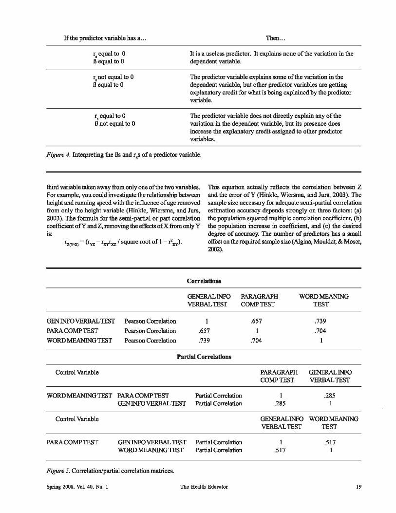
The bivariate correlation and partial correlation matrices for three of the variables discussed earlier (paragraph Comprehension Test scores, General Information Verbal Test scores, and Word Meaning Test scores) are presented in Figure 5. Notice that the correlation between Paragraph Comprehension Test scores and General Information Verbal Test scores is rather strong (r ~ .657), as is the correlation between Word Meaning Test scores and General Information test scores (r ~ .739). However, when the influence of each is removed from one another, the correlation between Word Meaning test scores and General Information Verbal test scores stays relatively strong (r ~ .517); whereas, the correlation between Paragraph Comprehension scores and General Information Verbal Test scores drops noticeably (r ~ .285). From these partial correlations, we can see that, although both variables are highly correlated with the General Information Verbal test scores, the Word Meaning Test scores remain highly correlated when the influence of Paragraph Comprehension scores is removed from consideration. The same can not be said for Word Meaning test scores, as much ofits correlation with General Infimuation Verbal test scores is lost when the influence ofWord Meaning Test scores is removed. From this analysis of the partial correlations, we can vest considerable confidence that the correlation between the Word Meaning Test scores and General Information Verbal Test scores is far superior to the correlation between Paragraph Comprehension scores and General Information Verbal Test scores.

A semi-partial correlation or part correlation is the correlation between two variables with the influence of a

Spring 2008, Vol. 40, No.1 The Health Educator 17

SPSS Syntax for computing structure coefficients

COMPUTEyhat~21.205+t9· .886+t6· .965 + tl5' -.034. EXECUlE. COMPUTE e ~ t5 - yhat. EXECUlE.

list variables ~ t9 t6 tl5 t5 yhat e.

CORRELATIONS NARIABLES~t9t6t15 t5 yhate IPRINT~TWOTAILNOSIG

IMISSING=PAIRWISE.

R RSquare

764 .584

SPSSOutput

Regression Model Summary

Adjusted R Square

.580

Std. Error of the Estimate

8.027

Predictors: MEMORY OF TARGET NUMBERS, WORD MEANING TEST, PARAGRAPH COMPREHENSION TEST; Dependent Variable: GENERAL INFORMATION VERBAL TEST

(Constant)

WORD MEANING TEST

PARAGRAPHCOMPTEST

MEMORYOFNUMBERS

Beta Weights

Unstandardized Standardized Coefficients Coefficients

B SE Beta

21.205 (a) 5.482

.886 .085 .549

.965 .187 .272

-.034 .060 -.021

Dependent Variable: GENERAL INFORMATION VERBAL TEST

Structure Coefficients

PARACOMP MEMOF

t

3.868

10.404

5.154

-.559

WORDMEANING

TEST TEST NUMBERS

WMEANTEST I .704" .052

PC TEST .704" I .069

MEMOFNUM .052 .069 I

GIVTEST .739" .657" .026

yhat C·967** .860** .034 :=> "Correlation is significant at the 0.01 level

Figure 3. Interpreting beta weights and structure coefficients.

18 The Health Educator

Sig.

.000

.000

.000

.577

GENINFO yhat

VERBALTEST

.739" .967"

.657" .860"

.026 .034

I .764"

.764" I

Spring 2008, Vol. 40, No. 1

If the predictor variable has a ...

r, equal to 0 a equal to 0

r,not equal to 0 a equal to 0

r, equal to 0 a not equal to 0

Then ...

It is a useless predictor. It explains none of the variation in the dependent variable.

The predictor variable explains some of the variation in the dependent variable, but other predictor variables are getting explanatory credit for what is being explained by the predictor variable.

The predictor variable does not directly explain any of the variation in the dependent variable, but its presence does increase the explanatory credit assigned to other predictor variables.

Figure 4. Interpreting the as and rss of a predictor variable.

third variable taken away from only one of the two variables. For example, you conld investigate the relationship between height and running speed with the influence of age removed from only the height variable (Hinkle, Wiersma, and Jurs, 2003). The formula for the semi-partial or part correlation coefficient ofY and Z, removing the effects of X from only Y is:

rZ(Y.X) ~ (ryz - r"",xz / square root of I - r xy)'

This equation actually reflects the correlation between Z and the error ofY (Hinkle, Wiersma, and Jurs, 2003). The sample size necessary for adequate semi-partial correlation estimation accuracy depends strongly on three factors: (a) the population squared multiple correlation coefficient, (b) the population increase in coefficient, and (c) the desired degree of accuracy. The number of predictors has a small effect on the required sample size (AJgina, Moulder, & Moser, 2002).

GEN INFO VERBAL TEST Pearson Correlation

PARA COMP TEST Pearson Correlation

WORD MEANING TEST Pearson Correlation

Control Variable

Correlations

GENERALINFO VERBALTEST

I

.657

.739

Partial Correlations

PARAGRAPH COMPTEST

.657

1

.704

PARAGRAPH COMPTEST

WORD MEANING TEST PARACOMPTEST Partial Correlation 1 GEN INFO VERBAL TEST Partial Correlation .285

WORD MEANING TEST

.739

.704

1

GENERALINFO VERBAL TEST

.285 1

Control Variable GENERALINFO WORD MEANING VERBAL TEST TEST

PARA COMP TEST GENINFO VERBAL TEST Partial Correlation 1 .517 WORD MEANING TEST Partial Correlation .517 1

Figure 5. Correlation/partial correlation matrices.

Spring 2008, Vol. 40, No.1 The Health Educator 19

Implications for Helllth Education Research

As noted by Bubi (2005), there is a paucity of articles related to statistics or measurement in health education. Unlike other fields within the social sciences, health education has been conspicuously absent from the dialogue surrounding the implementation and interpretation of various statistical analyses. While analyses such as regression are frequently employed by health education researchers, scholars in health education should be able to understand and explain the variety of regression coefficients which can be analyzed. The lack of scholarly discussion in the field (regarding the interpretation of statistical coefficients) discourages empirical knowledge generation and encourages simply memorizing procedures to produce numerical indices.

The health education profession must strive to generate, report, and interpret various regression coefficients accurately and adroitly, so that data explication appropriately reflects the reality we wish to purport. There has been discussion regarding the interpretation of effect sizes in health education research (Bubi, 2005; Merrill, Stoddard, and Shields, 2004; Watkins, Rivers, Rowell, Green, & Rivers, 2006), and it is suggested that similar recommendations stress the importance of computing structure coefficients to complement traditional beta weight coefficients. Through this practice, health educators will be able to more accurately distioguish independent variables which are responsible for impacting our dependent health behaviors of interest. For health education to improve its position as a science, it must embrace the practice of these analytic interpretations. Mandating the need to accurately report and interpret regression coefficients in all realms of health education research is essential to advancing result efficacy in the field.

Conclusion

There are a variety of coefficients used in simple and multiple regression analysis. It is important for health education researchers to not only understand what these coefficients are, but also understand what each represents and how each is computed and interpreted. Interpreting coefficients, such as regression coefficients (Pearson f,

Pearson:r2, R2, a, b, 8, rs,:r2s partial correlation and semi­partial correlation), allows the informed health education researcher to better understand the dynamics ofhis/her data. Consultiog these types of coefficients can provide health education research with further insight into correlations between variables of interest.

References

Algina, J., Moulder, B. C., Moser, B. K. (2003). Sample size requirements for accurate estimation of squared semi­partial correlation coefficients. Multivariate Behavioral Research, 37(1), 37-57.

Bubi, E. R (2005). The insignificance of "significance" tests: Three recommendations for health education researchers. American Journal of Health Education, 36,109-112.

Courville, T., & Thompson, B. (2001). Use of strocture coefficients in published multiple regression articles: Ii is not enough. Educational and Psychological Measurement, 61, 229-248.

Hetzel, R D. (1996).Aprimer on fuctor analysis with comments on pattems of practice and reporting. In B. Thompson (Ed.), Advances in social science methodology (Vol. 4). Greenwich, CT: JAI Press.

Hinkle,D.E., Wiersma, w.,Jurs, S. G (2003).Appliedstatistics for the behavioral sciences. Boston: Houghton Mifflin Company.

Holzinger, K. J., & Swineford, F. (1939). A study infactor analysis: The stability of a bi-factor solution (No. 48). Chicago, IL: University of Chicago.

Huck, S. W. (2004). Reading statistics and research (4th ed.). Boston: Pearson Education Inc.

Merrill, R M., Stoddard, J., Shields, E. C. (2004). The use of statistics in the American Journal of Health Education from 1994 through 2003: A content analysis. American Journal of Health Education, 35, 290-297.

Pedhazur, E. J. (1982). Multiple regression in behavioral research: Explanation and prediction (2nd ed.). New York: Holt, Rinehart & Wmston.

SPSS, Inc. (2006). SPSS Version 14.0. Chicago, IL: SPSS Incorporated.

Thompson, B. (2004). Exploratory and co11firmatory factor analysis: Understanding concepts and applications. Washington, DC: American Psychological Association.

Thompson, B. (2006). Foundations of behavioral statistics: An insight-based approach. New York: The Gnilford Press.

Thompson, B., & Borrello, G. M. (1985). The importance of structure coefficients in regression research. Educational and Psychological Measurement, 45, 203-209.

Watkins, D. C., Rivers, D., Rowell, K. L., Green, B. L., & Rivers, B. (2006). A closer look at effect sizes and their relevance to health education. American Journal of HealthEducation,37,103-108.

20 The Health Educator Spring 2008, Vol. 40, No. 1