a two–parameter sujatha distributionpoisson–sujatha distribution (psd), a poisson mixture of...

Submit Manuscript | http://medcraveonline.com

IntroductionThe statistical analysis and modeling of lifetime data are crucial

for statisticians working in various field of knowledge including medical science, engineering, social science, behavioral science, insurance, finance, among others. The classical one parameter lifetime distribution in statistics which were popular for modeling lifetime data are exponential distribution and Lindley distribution proposed by Lindley.1 Shanker et al.2 have detailed critical study on applications of exponential and Lindley distributions for modeling lifetime data from engineering and biomedical science and observed that exponential and Lindley distributions are not always suitable due to theoretical or applied point of view and presence of single parameter. In search for a lifetime distribution which gives a better fit than exponential and Lindley distributions, Shanker3 has proposed a new lifetime distribution named Sujatha distribution defined by its probability density function (pdf) and cumulative distribution function (cdf).

( )3

21 2( ; ) 1 ; 0, 0

2xf x x x e xθθ

θ θθ θ

−= + + > >+ + (1.1)

(1.2)

where θ is a scale parameter. It has been shown by Shanker3 that Sujatha distribution is a convex combination of exponential (θ) distribution, a gamma (2, θ) distribution and a gamma (3, θ) distribution. The first four moments about origin and central moments of Sujatha distribution obtained by Shanker3 are

( )2

1 2

2 6

2

θ θµ

θ θ θ′

+ +=

+ +

( )( )2

2 2

2 3 122 2

θ θµ

θ θ θ′

+ +=

+ +

( )( )2

3 3 2

6 4 20

2

θ θµ

θ θ θ′

+ +=

+ +

( )( )

2

4 2

24 5 304 2

θ θµ

θ θ θ′

+ +=

+ +

( )

4 3 2

2 22 2

4 18 12 12

2

θ θ θ θµ

θ θ θ

+ + + +=

+ +

( )( )

6 5 4 3 2

3 33 2

2 6 36 44 54 36 24

2

θ θ θ θ θ θµ

θ θ θ

+ + + + + +=

+ +

( )( )

8 7 6 5 4 3 2

4 44 2

3 3 24 172 376 736 864 912 480 240

2

θ θ θ θ θ θ θ θµ

θ θ θ

+ + + + + + + +=

+ +

Shanker3 has discussed its important properties including shapes of density function for varying values of parameter, hazard rate function, mean residual life function, stochastic ordering, mean deviations, Bonferroni and Lorenz curves, and stress–strength reliability. Shanker3 discussed the maximum likelihood estimation of parameter and showed applications of Sujatha distribution to model lifetime data from biomedical science and engineering. Shanker4 has introduced Poisson–Sujatha distribution (PSD), a Poisson mixture of Sujatha distribution, and studied its properties, estimation of parameter and applications to model count data. Shanker & Hagos5 have discussed zero–truncated Poisson– Sujatha distribution (ZTPSD) and applications for modeling count data excluding zero counts. Shanker & Hagos6 have also studied size–biased Poisson– Sujatha distribution and its applications for count data excluding zero counts.

The Lindley distribution and a size–biased Lindley distribution (SBLD) having parameter θ are defined by their pdf

( )

2

2 ( ; ) 1 ; 0, 01

xf x x e xθθθ θ

θ

−= + > >+ (1.3)

( )

3

3 ( ; ) 1 ; 0, 02

xf x x x e xθθθ θ

θ

−= + > >+ (1.4)

Ghitany et al.7 have discussed various statistical and mathematical properties, estimation of parameter and application of Lindley distribution to model waiting time data in a bank and it has been showed that Lindley distribution provides better fit than exponential distribution.

In this paper, a two–parameter Sujatha distribution (TPSD), which

Biom Biostat Int J. 2018;7(3):188‒197. 188© 2018 Tesfay et al. This is an open access article distributed under the terms of the Creative Commons Attribution License, which permits unrestricted use, distribution, and build upon your work non-commercially.

A two–parameter Sujatha distributionVolume 7 Issue 3 - 2018

Mussie Tesfay, Rama ShankerDepartment of Statistics, Eritrea Institute of Technology Asmara, Eritrea

Correspondence: Rama Shanker, Department of Statistics, College of Science, Eritrea Institute of Technology, Asmara, Eritrea, Email [email protected], [email protected]

Received: March 15, 2018 | Published: May 10, 2018

Abstract

This paper proposes a two–parameter Sujatha distribution (TPSD). This includes size–biased Lindley distribution and Sujatha distribution as particular cases. Its important statistical properties including shapes of density function for varying values of parameters, coefficient of variation, skewness, kurtosis, index of dispersion, hazard rate function, mean residual life function, stochastic ordering ,mean deviations, Bonferroni and Lorenz curves, and stress–strength reliability have been discussed. The estimation of parameters has been discussed using the method of moments and the method of maximum likelihood. Application of the distribution has been discussed with a real lifetime data.

Keywords: Sujatha distribution, moments, statistical properties, estimation of parameters, application

Biometrics & Biostatistics International Journal

Research Article Open Access

( ) ( )1

2; 1 1 ; 0, 02 2

xx xF x e xθθ θ θ

θ θθ θ

−+ += − + > >

+ +

https://creativecommons.org/licenses/by-nc/4.0/

http://crossmark.crossref.org/dialog/?doi=10.15406/bbij.2018.07.00208&domain=pdf

A two–parameter Sujatha distribution 189Copyright:

©2018 Tesfay et al.

Citation: Tesfay M, Shanker R. A two–parameter Sujatha distribution. Biom Biostat Int J. 2018;7(3):188‒197. DOI: 10.15406/bbij.2018.07.00208

includes size–biased Lindley distribution and Sujatha distribution as particular cases, has been proposed. Its important statistical properties including coefficient of variation, skewness, kurtosis, index of dispersion, hazard rate function, mean residual life function, stochastic ordering, mean deviations, Bonferroni and Lorenz curves, stress–strength reliability have been discussed. The estimation of the parameters has been discussed using method of moments and maximum likelihood estimation. A numerical example has been given to test the goodness of fit of TPSD over Lindley and Sujatha distributions.

A two–parameter Sujatha distributionA Two parameter Sujatha distribution (TPSD) having parameters

θ and α is defined by its pdf

( )3

24 2( ; , ) ; 0, 0, 0

2xf x x x e xθθ

θ α α θ ααθ θ

−= + + > > ≥+ +

(2.1)

where θ is a scale parameter and is α is a shape parameter. It can be easily verified that (2.1) reduces to Sujatha distribution (1.1) and SBLD (1.4) for α = 1 and α = 0 respectively.

Like Sujatha distribution (1.1), TPSD (2.1) is also a convex combination of exponential (θ ), gamma (2, θ ) and gamma (3,θ ) distributions. We have

( ) ( ) ( ) ( ) ( )4 1 1 2 2 1 2 3; , , , 1 ,f x p g x p g x p p g xθ α θ θ θ= + + − − (2.2)

where

( )2

1 2 12 2, , , ; 0, 02 2

xp p g x e xθαθ θθ θ θ

αθ θ αθ θ

−= = = > >+ + + +

( ) ( ) ( ) ( )2 3

2 1 3 12 3, ; 0, 0, , ; 0, 0.

2 3x xg x e x x g x e x xθ θθ θ

θ θ θ θ− − − −= > > = > >Γ Γ

The corresponding cdf of TPSD (2.1) can be obtained as

(2.3)

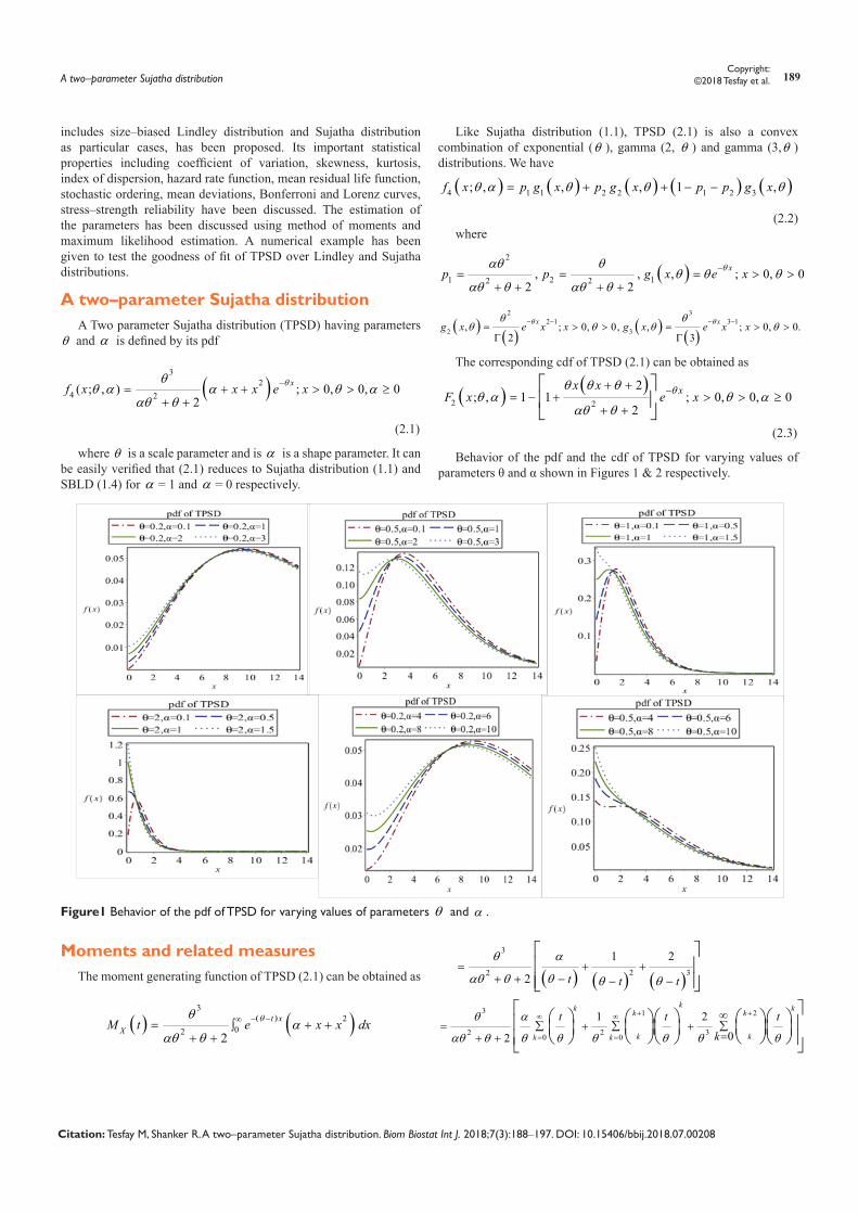
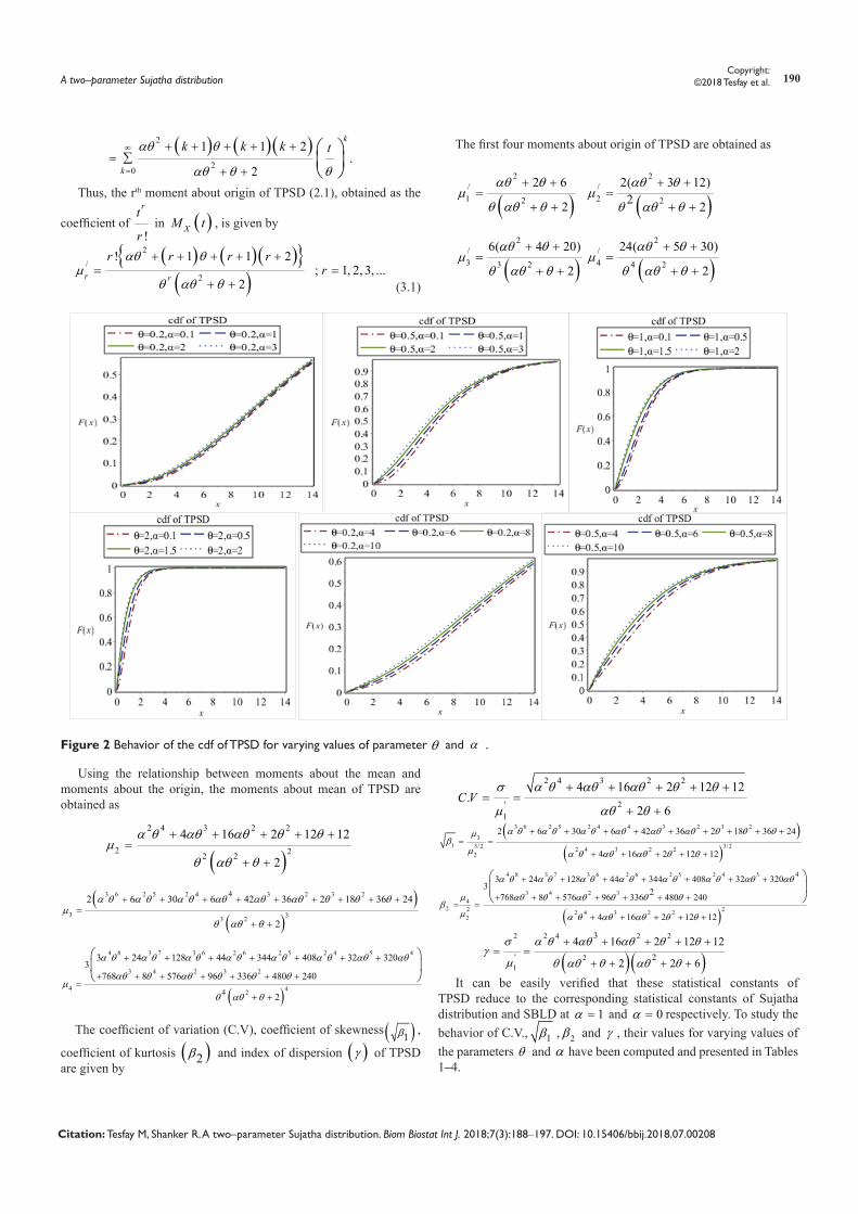
Behavior of the pdf and the cdf of TPSD for varying values of parameters θ and α shown in Figures 1 & 2 respectively.

Figure1 Behavior of the pdf of TPSD for varying values of parameters θ and α .

Moments and related measuresThe moment generating function of TPSD (2.1) can be obtained as

( ) ( ) ( )

32

02 2t x

XM t e x x dxθθα

αθ θ

− −∞= + +∫+ +

( ) ( ) ( )

3

2 32

1 2

2 t t t

θ α

αθ θ θ θ θ= + +

+ + − − −

3 1 2

2 2 30 0

1 2

02

kk kk k

k kk k

t t t

k

θ α

αθ θ θ θ θ θ θ θ

+ +∞ ∞

= =

∞∑ ∑ ∑= + +

=+ +

( ) ( )2 2

2; , 1 1 ; 0, 0, 0

2xx x

F x e xθθ θ θθ α θ α

αθ θ

−+ += − + > > ≥

+ +

https://doi.org/10.15406/bbij.2018.07.00208




Thus, the rth moment about origin of TPSD (2.1), obtained as the

coefficient of !

rt

r in ( )XM t , is given by

(3.1)

The first four moments about origin of TPSD are obtained as

( )2

/1 2

2 6

2

αθ θµ

θ αθ θ

+ +=

+ +

( )2

/2 2

2( 3 12)2 2

αθ θµ

θ αθ θ

+ +=

+ +

( )2

/3 3 2

6( 4 20)

2

αθ θµ

θ αθ θ

+ +=

+ + ( )2

/4 4 2

24( 5 30)

2

αθ θµ

θ αθ θ

+ +=

+ +

Figure 2 Behavior of the cdf of TPSD for varying values of parameter and .θ α

Using the relationship between moments about the mean and moments about the origin, the moments about mean of TPSD are obtained as

( )2 4 3 2 2

2 22 2

4 16 2 12 12

2

α θ αθ αθ θ θµ

θ αθ θ

+ + + + +=

+ +

( )( )

3 6 2 5 2 4 3 2 3 2

3 33 2

42 6 30 6 42 36 2 18 36 24

2

α θ α θ α θ αθ αθ αθ θ θ θµ

θ αθ θ

+ + + + + + + + +=

+ +

( )

4 8 3 7 3 6 2 6 2 5 2 4 5 4

3 4 2 3 2

4 424

3 24 128 44 344 408 32 3203

768 8 576 96 336 480 240

2

α θ α θ α θ α θ α θ α θ αθ αθ

αθ θ αθ θ θ θµ

θ αθ θ

+ + + + + + +

+ + + + + + +=

+ +

The coefficient of variation (C.V), coefficient of skewness ( )1β ,

coefficient of kurtosis ( )2β and index of dispersion ( )γ of TPSD are given by

2 4 3 2 2

' 21

4 16 2 12 12.

2 6C V

σ α θ αθ αθ θ θ

µ αθ θ

+ + + + += =

+ +

( )( )

3 6 2 5 2 4 4 3 2 3 2

31 3/23/2 2 4 3 2 2

2

2 6 30 6 42 36 2 18 36 24

4 16 2 12 12

α θ α θ α θ αθ αθ αθ θ θ θµβ

µ α θ αθ αθ θ θ

+ + + + + + + + += =

+ + + + +

( )

4 8 3 7 3 6 2 6 2 5 2 4 5

3 4 2 34

2 22 2 4 3 2 22

43 24 128 44 344 408 32 3203 2768 8 576 96 336 480 240

4 16 2 12 12

α θ α θ α θ α θ α θ α θ αθ αθ

µ αθ θ αθ θ θ θβ

µ α θ αθ αθ θ θ

+ + + + + + +

+ + + + + + += =

+ + + + +

( )( )

2 2 4 2 2

' 21

3

2

4 16 2 12 12

2 2 6

σ α θ αθ αθ θ θγ

µ θ αθ θ αθ θ

+ + + + += =

+ + + +

It can be easily verified that these statistical constants of TPSD reduce to the corresponding statistical constants of Sujatha distribution and SBLD at 1α = and 0α = respectively. To study the behavior of C.V., 1β , 2β and γ , their values for varying values of the parameters θ and α have been computed and presented in Tables 1–4.

( ) ( )( )2

20

1 1 2.

2

k

k

k k k tαθ θ

αθ θ θ

∞

=

+ + + + +∑=

+ +

( ) ( )( ){ }( )

2/

2

! 1 1 2; 1, 2, 3, ...

2r r

r r r rr

αθ θµ

θ αθ θ

+ + + + += =

+ +





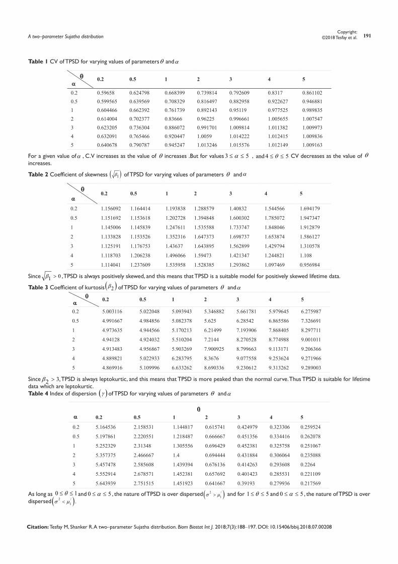
Table 1 CV of TPSD for varying values of parametersθ andα

θα

0.2 0.5 1 2 3 4 5

0.2 0.59658 0.624798 0.668399 0.739814 0.792609 0.8317 0.8611020.5 0.599565 0.639569 0.708329 0.816497 0.882958 0.922627 0.9468811 0.604466 0.662392 0.761739 0.892143 0.95119 0.977525 0.9898352 0.614004 0.702377 0.83666 0.96225 0.996661 1.005655 1.0075473 0.623205 0.736304 0.886072 0.991701 1.009814 1.011382 1.0099734 0.632091 0.765466 0.920447 1.0059 1.014222 1.012415 1.0098365 0.640678 0.790787 0.945247 1.013246 1.015576 1.012149 1.009163

For a given value ofα , C.V increases as the value of θ increases .But for values 3 5α≤ ≤ , and 4 5θ≤ ≤ CV decreases as the value of θ increases.

Table 2 Coefficient of skewness ( )1β of TPSD for varying values of parameters θ andα

θ

α 0.2 0.5 1 2 3 4 5

0.2 1.156092 1.164414 1.193838 1.288579 1.40832 1.544566 1.694179

0.5 1.151692 1.153618 1.202728 1.394848 1.600302 1.785072 1.947347

1 1.145006 1.145839 1.247611 1.535588 1.733747 1.848046 1.912879

2 1.133828 1.153526 1.352316 1.647373 1.698737 1.653874 1.586127

3 1.125191 1.176753 1.43637 1.643895 1.562899 1.429794 1.310578

4 1.118703 1.206238 1.496066 1.59473 1.421347 1.244821 1.108

5 1.114041 1.237609 1.535958 1.528385 1.293862 1.097469 0.956984

Since 01β > , TPSD is always positively skewed, and this means that TPSD is a suitable model for positively skewed lifetime data.

Table 3 Coefficient of kurtosis ( )2β of TPSD for varying values of parameters θ andα

θ α

0.2 0.5 1 2 3 4 5

0.2 5.003116 5.022048 5.093943 5.346882 5.661781 5.979645 6.275987

0.5 4.991667 4.984856 5.082378 5.625 6.28542 6.865586 7.326691

1 4.973635 4.944566 5.170213 6.21499 7.193906 7.868405 8.297711

2 4.94128 4.924032 5.510204 7.2144 8.270528 8.774988 9.001011

3 4.913483 4.956867 5.903269 7.900925 8.799663 9.113171 9.206366

4 4.889821 5.022933 6.283795 8.3676 9.077558 9.253624 9.271966

5 4.869916 5.109996 6.633262 8.690336 9.230612 9.313262 9.289003

Since 3,2β > TPSD is always leptokurtic, and this means that TPSD is more peaked than the normal curve. Thus TPSD is suitable for lifetime data which are leptokurtic.Table 4 Index of dispersion ( )γ of TPSD for varying values of parameters θ andα

θα 0.2 0.5 1 2 3 4 5

0.2 5.164536 2.158531 1.144817 0.615741 0.424979 0.323306 0.259524

0.5 5.197861 2.220551 1.218487 0.666667 0.451356 0.334416 0.262078

1 5.252329 2.31348 1.305556 0.696429 0.452381 0.325758 0.251067

2 5.357375 2.466667 1.4 0.694444 0.431884 0.306064 0.235088

3 5.457478 2.585608 1.439394 0.676136 0.414263 0.293608 0.2264

4 5.552914 2.678571 1.452381 0.657692 0.401423 0.285531 0.221109

5 5.643939 2.751515 1.451923 0.641667 0.39193 0.279936 0.217569

As long as 0 1θ≤ ≤ and 0 5α≤ ≤ , the nature of TPSD is over dispersed ( )2 /1σ µ> and for 1 5θ≤ ≤ and 0 5α≤ ≤ , the nature of TPSD is over

dispersed ( )2 /1 .σ µ<





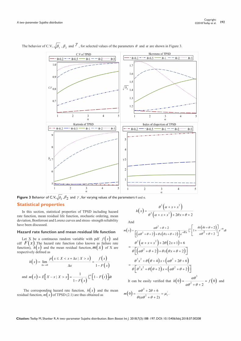
The behavior of C.V., 1β , 2β and γ , for selected values of the parameters θ and α are shown in Figure 3.

Figure 3 Behavior of C.V., 1β , 2β and γ , for varying values of the parameters θ and α.

Statistical propertiesIn this section, statistical properties of TPSD including hazard

rate function, mean residual life function, stochastic ordering, mean deviation, Bonferroni and Lorenz curves and stress–strength reliability have been discussed.

Hazard rate function and mean residual life function

Let X be a continuous random variable with pdf ( )f x and cdf ( )F x .The hazard rate function (also known as failure rate function), ( )h x and the mean residual function, ( )m x of X are respectively defined as

and ( ) [ ] ( ) ( )1| 1

1xm x E X x X x F t dt

F x∞= − > = −∫

−

The corresponding hazard rate function, ( )h x and the mean residual function, ( )m x of TPSD (2.1) are thus obtained as

( ) ( )( )2

3 2

2 2 2

x xh x

x x x

θ α

θ α θ θ

+ +=

+ + + + +

And

( ) ( ) ( )( )2

2

221 2 22 2

tx

t tm x e dtxx x e

θθ θ θαθ θθ αθ θαθ θ θ θ θ

−∞ + ++ += +∫− + ++ + + + +

( ) ( )( ) ( )

2 2

2

2 2 1 6

2 2

x x x

x x

θ α θ

θ αθ θ θ θ θ

+ + + + +=

+ + + + +

( ) ( )( ) ( )

2 2 2

2 2 2

4 2 6

2 2

x x

x x

θ θ θ αθ θ

θ θ θ θ αθ θ

+ + + + +=

+ + + + +

It can be easily verified that ( ) ( )3

20 02

h fαθ

αθ θ= =

+ + and

( )2

/12

2 60 .

( 2)m

αθ θµ

θ αθ θ

+ += =

+ +

( ) ( ) ( )( )0

|lim

1x

p x X x x X x f xh x

x F x∆ →

≤ < + ∆ >= =

∆ −





It can also be easily verified that the expression of ( )h x and ( )m xof TPSD reduce to the corresponding ( )h x and m(x) of Sujatha distribution at 1.α =

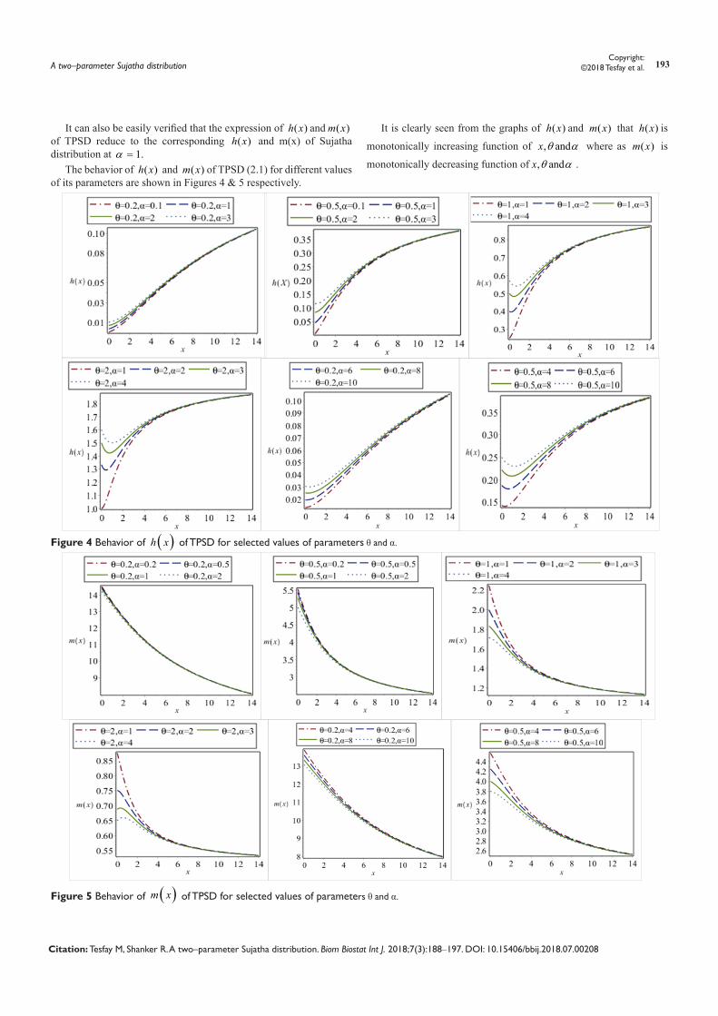
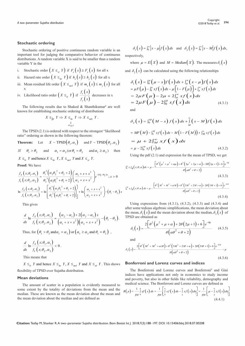
The behavior of ( )h x and ( )m x of TPSD (2.1) for different values of its parameters are shown in Figures 4 & 5 respectively.

It is clearly seen from the graphs of ( )h x and ( )m x that ( )h x is

monotonically increasing function of , andx θ α where as ( )m x is

monotonically decreasing function of , andx θ α .

Figure 4 Behavior of ( )h x of TPSD for selected values of parameters θ and α.

Figure 5 Behavior of ( )m x of TPSD for selected values of parameters θ and α.





Stochastic ordering

Stochastic ordering of positive continuous random variable is an important tool for judging the comparative behavior of continuous distributions. A random variable X is said to be smaller than a random variable Y in the

i. Stochastic order ( )stX Y≤ if ( ) ( )x yF x F x≥ for all x

ii. Hazard rate order ( )hrX Y≤ if ( ) ( )x yh x h x≥ for all x

iii. Mean residual life order ( )mrlX Y≤ if ( ) ( )x ym x m x≤ for all x

iv. Likelihood ratio order ( )lrX Y≤ if ( )( )

x

y

f x

f x decreases in x

The following results due to Shaked & Shanthikumar8 are well known for establishing stochastic ordering of distributions

.hr mlr

x yst

X Y X Y X Ylr⇓≤

≤ ⇒ ≤ ⇒ ≤

The TPSD (2.1) is ordered with respect to the strongest “likelihood ratio” ordering as shown in the following theorem:

Theorem: Let ( )1 1~ TPSD ,X θ α and ( )2 2~ TPSD ,Y θ α

.If 1 2θ θ> and 1 2α α= (or 1 2θ θ= and 1 2α α≥ ) then

and hence , and .lr hr mrl stX Y X Y X Y X Y≤ ≤ ≤ ≤

Proof: We have

( )( )

( )( )

( )3 2 2

1 2 2 21 1 1 1 223 2

2 22 1 1 12

2; ,; 0

; , 2

xX

Y

f x x xe x

f x x x

θ θθ α θ θθ α α

θ α αθ α θ θ

− −+ + + +

= >+ ++ +

( )( )

( )( ) ( )

1

3 2 21 2 2 21 1 1

1 23 22 2 22 1 1

2

2; ,ln ln ln

; , 2

X

Y

f x x xx

f x x x

θ α θ θθ α αθ θ

θ α αθ α θ θ

+ + + += + − −

+ ++ +

This gives

( )( )

( ) ( )( )( ) ( )1 1 2 1 2 1

1 22 22 2 1 2

; , 2ln .

; ,X

Y

f x xd

dx f x x x x x

θ α α α α αθ θ

θ α α α

− + −= − −

+ + + +

Thus, for ( ) ( )1 2 1 2 1 2 1 2and or andθ θ α α α α θ θ> = ≥ = ,

( )( )

1 1

2 2

; ,ln 0 .

; ,X

Y

f xd

dx f x

θ α

θ α<

This means that

and hence , andlr hr mrl stX Y X Y X Y X Y≤ ≤ ≤ ≤ . This shows

flexibility of TPSD over Sujatha distribution.

Mean deviations

The amount of scatter in a population is evidently measured to some extent by the totality of deviations from the mean and the median. These are known as the mean deviation about the mean and the mean deviation about the median and are defined as

( ) ( )01 x x f x dxδ µ∞= −∫ and ( ) ( )02 ,x x M f x dxδ ∞= −∫

respectively,

where ( )E Xµ = and ( ).M Median X= The measures ( )1 xδ

and ( )2 xδ can be calculated using the following relationships

( ) ( ) ( ) ( ) ( )01 x x f x dx x f x dxµµδ µ µ∞= − + −∫ ∫

( ) ( ) ( ) ( )0 1F x f x dx F x f x dxµµµ µ µ µ ∞= − − − +∫ ∫

( ) ( )2 2 2F x f x dxµµ µ µ ∞= − + ∫

( ) ( )02 2F x f x dxµµ µ= − ∫ (4.3.1)

and

( ) ( ) ( ) ( ) ( )02M

Mx M x f x dx x M f x dxδ

∞

= − + −∫ ∫

( ) ( ) ( )( ) ( )0 1MMMF M x f x dx M F M x f x dx∞= − − − +∫ ∫

( )2 M x f x dxµ ∞= + ∫

( )02 M x f x dxµ= − ∫ (4.3.2)

Using the pdf (2.1) and expression for the mean of TPSD, we get

( )( ) ( ) ( )

( )3 3 2 2 2

0 2

3 2 2 3 1 6; ,4 2

ex f x dx

θµ

µθ µ µ αµ θ µ µ α θ µ

θ α µθ αθ θ

−+ + + + + + + += −∫

+ +

(4.3.3)

( )( ) ( ) ( )

( )3 3 2 2 2

0 2

3 2 2 3 1 6; ,4 2

M

MM M M M M M e

x f x dx

θθ α θ α θθ α µ

θ αθ θ

−+ + + + + + + += −∫

+ +

(4.3.4)

Using expressions from (4.3.1), (4.3.2), (4.3.3) and (4.3.4) and after some tedious algebraic simplifications, the mean deviation about the mean, ( )1 xδ and the mean deviation about the median, ( )2 xδ of TPSD are obtained as

( )( ) ( )

( )2 2

1 2

2 2 2 1 6

2

ex

θµθ µ µ α θ µδ

θ αθ θ

−+ + + + +=

+ +

(4.3.5)

and

( )( ) ( ) ( )

( )3 3 2 2 2

2 2

2 3 2 2 3 1 6

2

MM M M M M M ex

θθ α θ α θδ µ

θ αθ θ

−+ + + + + + + += −

+ +

(4.3.6)Bonferroni and Lorenz curves and indices

The Bonferroni and Lorenz curves and Bonferroni9 and Gini indices have applications not only in economics to study income and poverty, but also in other fields like reliability, demography and medical science. The Bonferroni and Lorenz curves are defined as

(4.4.1)

( ) ( ) ( ) ( ) ( )0 0

1 1 1q

q qB p xf x dx x f x dx x f x dx x f x dx

p p pµ

µ µ µ

∞ ∞ ∞

= = − = −∫ ∫ ∫ ∫





and

( ) ( ) ( ) ( ) ( )0 0

1 1 1q

q qL p x f x dx x f x dx x f x dx x f x dxµ

µ µ µ

∞ ∞ ∞

= = − = −∫ ∫ ∫ ∫

(4.4.2)

respectively or equivalently.

( ) ( )1

0

1 pB p F x dx

pµ−= ∫ (4.4.3)

and ( ) ( )1

0

1 pL p F x dx

µ

−= ∫ (4.4.4)

respectively, where ( )E xµ = and ( )1q F p−= .

The Bonferroni and Gini indices are thus defined as

( )

1

01B B p dp= − ∫ (4.4.5)

and ( )1

01 2G L p dp= − ∫ (4.4.6)

respectively.

Using pdf of TPSD (2.1), we get

( ) ( ) ( ) ( )( )

3 3 2 2

2

2{ 3 2 2 3 1 6}

2 6

q

q

q q q q q q ex f x dx

θθ α θ α θ

θ αθ θ

−∞ + + + + + + + +

=∫+ +

(4.4.7)

Now using equation (4.4.7), (4.4.1) and (4.4.2), we get

( ) ( ) ( ) ( )3 3 2 2 2

2

{ 3 2 2 3 1 6}11

2 6

qq q q q q q eB p

p

θθ α θ α θ

αθ θ

−+ + + + + + + += −

+ +

(4.4.8)

and

( ) ( ) ( ) ( )3 3 2 2 2

2

{ 3 2 2 3 1 6}1

2 6

qq q q q q q eL p

θθ α θ α θ

αθ θ

−+ + + + + + + += −

+ + (4.4.9)

Now using the equations (4.4.8) and (4.4.9) in (4.4.5) and (4.4.6), the Bonferroni and Gini indices of TPSD (2.1) are obtained as

( ) ( ) ( )3 3 2 2 2

2

{ 3 2 2 3 1 6}1

2 6

qq q q q q q eB

θθ α θ α θ

αθ θ

−+ + + + + + + += −

+ +

(4.4.10)

( ) ( ) ( )3 3 2 2 2

2

2{ 3 2 2 3 1 6}1

2 6

qq q q q q q eG

θθ α θ α θ

αθ θ

−+ + + + + + + += − +

+ +

(4.4.11)

Stress–strength reliability

The stress–strength reliability of a component illustrates the life of the component which has random strength that is subjected to random stress. When the stress of the component Y applied to it exceeds the strength of the component X, the component fails instantly and the component will function satisfactorily till X > Y . Therefore, R = P (Y < X ) is a measure of the component reliability and is known as stress–strength reliability in statistical literature. It has extensive application in almost all areas of knowledge especially in engineering such as structure, deterioration of rocket motor, static fatigue of ceramic component, aging of concrete pressure vessels etc.

Let X and Y be independent strength and stress random variables having TPSD (2.1) with parameter ( )1 1,θ α and ( )2 2,θ α respectively. Then the stress–strength reliability R of TPSD can be obtained as

( ) ( ) ( )0

| xR P Y X P Y X X x f x dx∞

= < = < =∫

( ) ( )1, 1 2, 20

; ;f x F x dxθ α θ α∞

= ∫

( ) ( )( )( )( )

1

6 5 2 41 2 2 1 2 1 2 2 1 1 1 1 2 1 2 1 2

2 2 3 31 1 1 1 1 2 1 1 2 1 23

1 3 3 2 2 2 4 21 2 1 1 1 2 1 1 1 1 2 1 2

3 2 21 1 1 1 1 1 2 1

2

1

1

1

( ) 2 4 7 3 6 2 6 3

9 3 18 4 7 4 202

5 20 2 5 30 40

10 12 20 21

α α θ α α α α θ θ α θ α θ α α α α θ θ

α θ α θ α θ α θ θ α α θ θθ

α θ α θ α θ α θ θ θ α α θ θ

α θ α θ θ θ θ θ α θ

+ + + + + + + + +

+ + + + + + +

+ + + + + + + +

+ + + + + += −

( )( )( )( )

2

1

21 1

52 21 1 2 2 11 2

2

2 2 2

θ θ

α θ θ α θ θ θ θ

+ +

+ + + + +

It can be verified that the stress–strength reliability of Sujatha distribution is a particular case of stress–strength reliability of TPSD at 1 2 1.α α= =

Estimation of parametersIn this section, the estimation of parameters of TPSD using the

method of moments and the method of maximum likelihood have been discussed.

Method of moment estimates (MOME)

Since TPSD (2.1) has two parameters to be estimated, the first two moments about the origin are required to estimate its parameters using method of moments. Equating the population mean to the sample mean, we have

( ) ( ) ( )2 2

2 2 2

2 6 2 4

2 2 2x

αθ θ αθ θ θ

θ αθ θ θ αθ θ θ αθ θ

+ + + + += = +

+ + + + + +

( )2

1 4

2x

θ

θ θ αθ θ

+= +

+ +

( )2 42

1x

θαθ θ

θ

++ + =

− (5.1.1)

Again equating the second population moment with the corresponding sample moment, we have





( )( )

( )( )

( )( )

2 2'2 22 2 2

2 3 12 2 2 4 52 2 22 2

mαθ θ αθ θ θ

θ αθ θθ αθ θ θ αθ θ

+ + + + += = +

+ ++ + + +

( )( )

( )( )

2'2 2 22 2 2

2 3 12 4 52

2 2m

αθ θ θ

θθ αθ θ θ αθ θ

+ + += = +

+ + + +

( )2' 22

4 52

2m

θαθ θ

θ

++ + =

− (5.1.2)

Equations (5.1.1) and (5.1.2) give the following cubic equation in θ

( ) ( )' 3 ' 22 24 2 10 1 12 0m m X Xθ θ θ+ − − − + = (5.1.3)

Solving equation (5.1.3) using any iterative method such as Newton–Raphson method, Regula–Falsi method or Bisection method, method of moment estimation (MOME) θ of θ can be obtained and substituting the value of θ in equation (5.1.1), MOME α of α can be obtained as

2

2

2( 1) 6

( 1)

x x

x

θ θα

θ θ

− − − +=

−

(5.1.4)

Maximum likelihood estimates (MLE)

Let ( )1 2 3, , , ... nx x x x be random sample from TPSD (2.1). The likelihood function L is given by

( )3

22

1,

2

n n xi i

i

n

L x x e θθα

αθ θ−

=∏= + +

+ +

where x is the sample mean.The natural log likelihood function is thus obtained as

( ) ( )2 2

1ln 3 ln ln 2 ln i i

i

nL n x x n xθ αθ θ α θ

=∑= − + + + + + −

The maximum likelihood estimate (MLE’s) ˆ ˆ( , )θ α of ( , )θ α are then the solutions of the following non–linear equations

( )2

2 1ln 30

2

nL nn x

αθ

θ θ αθ θ

+∂= − − =

∂ + + (5.2.1)

2

2

2 1

ln 10

2

n

ii i

L n

x x

θ

α αθ θ α=

∂∑= − + =

∂ + + + + (5.2.2)

These two natural log likelihood equations do not seem to be solved directly, because they cannot be expressed in closed forms. The (MLE’s) ˆ ˆ( , )θ α of ( , )θ α can be computed directly by solving the natural log likelihood equations using Newton–Raphson iteration method using R–software till sufficiently close values of ˆ ˆandθ α are

obtained. The initial values of parameters θ and α are the MOME ( , )θ α of the parameters ( , ).θ α

A numerical exampleIn this section an application of TPSD using maximum likelihood

estimates has been discussed with a real lifetime data set. The data set regarding vinyl chloride obtained from clean up gradient monitoring wells in mg/l, available in Bhaumik et al.10 has been considered. The data set is

5.1 1.2 1.3 0.6 0.5 2.4 0.5 1.1 8 0.8 0.4 0.6 0.9

0.4 2 0.5 5.3 3.2 2.7 2.9 2.5 2.3 1 0.2 0.1 0.1

1.8 0.9 2.4 6.8 1.2 0.4 0.2

In order to compare lifetime distributions, values of 2 ln L− , AIC (Akaike Information Criterion), BIC (Bayesian Information Criterion) and K–S Statistic (Kolmogorov–Smirnov Statistic) for the above data set has been computed. The formulae for computing AIC, BIC, and K–S Statistics are as follows:

2 ln 2AIC L k= − + , 2 ln lnBIC L k n= − + and

( ) ( )0Sup nx

D F x F x= − , where k = the number of parameters,

n = the sample size, and the ( )nF x = empirical distribution function. The best distribution is the distribution which corresponds to lower values of 2 ln L− , AIC, and K–S statistic and higher p–value. The

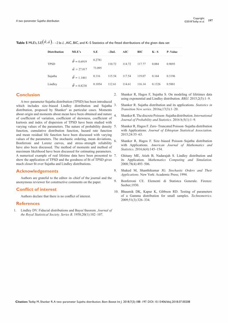
MLE ( )ˆ ˆ,θ α along with their standard errors, 2 ln L− , AIC, BIC, K–S Statistic and p–value of the fitted distributions are presented in the Table 5.

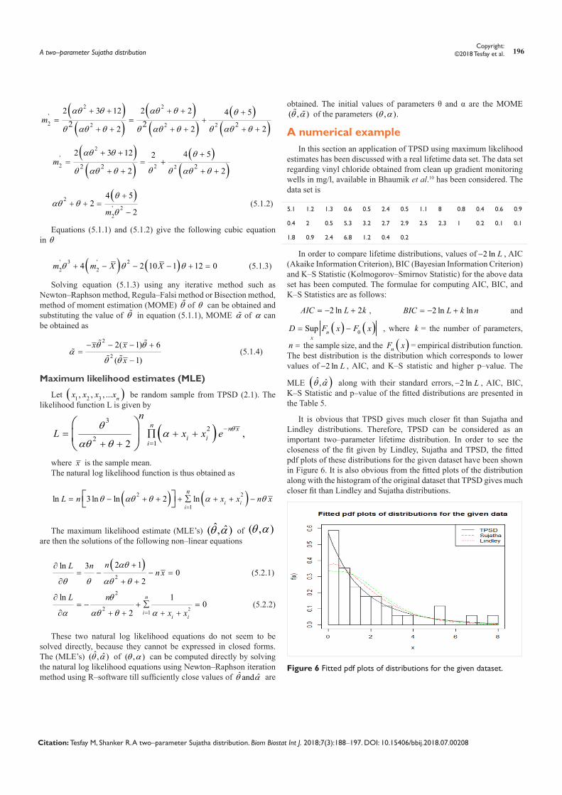
It is obvious that TPSD gives much closer fit than Sujatha and Lindley distributions. Therefore, TPSD can be considered as an important two–parameter lifetime distribution. In order to see the closeness of the fit given by Lindley, Sujatha and TPSD, the fitted pdf plots of these distributions for the given dataset have been shown in Figure 6. It is also obvious from the fitted plots of the distribution along with the histogram of the original dataset that TPSD gives much closer fit than Lindley and Sujatha distributions.

Figure 6 Fitted pdf plots of distributions for the given dataset.





Table 5 MLE’s, S.E ( )ˆ ˆ, ,θ α 2 ln L− , AIC, BIC, and K–S Statistics of the fitted distributions of the given data set

Distribution MLE’s S.E –2lnL AIC BIC K– S P–Value

TPSDθ̂ = 0.6919 0.2781

110.72 114.72 117.77 0.084 0.9693

α̂ = 27.017 73.095

Sujatha θ̂ = 1.1461 0.116 115.54 117.54 119.07 0.164 0.3196

Lindley θ̂ = 0.8238 0.1054 112.61 114.61 116.14 0.1326 0.5881

ConclusionA two–parameter Sujatha distribution (TPSD) has been introduced

which includes size–biased Lindley distribution and Sujatha distribution, proposed by Shanker3 as particular cases. Moments about origin and moments about mean have been obtained and nature of coefficient of variation, coefficient of skewness, coefficient of kurtosis and index of dispersion of TPSD have been studied with varying values of the parameters. The nature of probability density function, cumulative distribution function, hazard rate function and mean residual life function have been discussed with varying values of the parameters. The stochastic ordering, mean deviations, Bonferroni and Lorenz curves, and stress–strength reliability have also been discussed. The method of moments and method of maximum likelihood have been discussed for estimating parameters. A numerical example of real lifetime data have been presented to show the application of TPSD and the goodness of fit of TPSD gives much closer fit over Sujatha and Lindley distributions.

AcknowledgementsAuthors are grateful to the editor–in–chief of the journal and the

anonymous reviewer for constructive comments on the paper.

Conflict of interestAuthors declare that there is no conflict of interest.

References1. Lindley DV. Fiducial distributions and Bayes’theorem. Journal of

the Royal Statistical Society. Series B. 1958;20(1):102–107.

2. Shanker R, Hagos F, Sujatha S. On modeling of lifetimes data using exponential and Lindley distribution. BBIJ. 2015;2(5):1–9.

3. Shanker R. Sujatha distribution and its applications. Statistics in Transition New series. 2016a;17(3):1–20.

4. Shanker R. The discrete Poisson–Sujatha distribution. International Journal of Probability and Statistics. 2016 b;5(1):1–9.

5. Shanker R, Hagos F. Zero–Truncated Poisson–Sujatha distribution with Applications. Journal of Ethiopian Statistical Association. 2015;24:55–63.

6. Shanker R, Hagos F. Size–biased Poisson–Sujatha distribution with Applications. American Journal of Mathematics and Statistics. 2016;6(4):145–154.

7. Ghitany ME, Atieh B, Nadarajah S. Lindley distribution and its Application. Mathematics Computing and Simulation. 2008;78(4):493–506.

8. Shaked M, Shanthikumar JG. Stochastic Orders and Their Applications. New York: Academic Press; 1994.

9. Bonferroni CE. Elementi di Statistca Generale. Firenze: Seeber;1930.

10. Bhaumik DK, Kapur K, Gibbson RD. Testing of parameters of a Gamma distribution for small samples. Technometrics. 2009;51(3):326–334.


https://www.jstor.org/stable/2983909?seq=1#page_scan_tab_contents

https://www.jstor.org/stable/2983909?seq=1#page_scan_tab_contents

http://medcraveonline.com/BBIJ/BBIJ-02-00042.pdf

http://medcraveonline.com/BBIJ/BBIJ-02-00042.pdf

http://cejsh.icm.edu.pl/cejsh/element/bwmeta1.element.desklight-ecc31ede-da34-46c6-953a-4ec12ecbe8f2

http://cejsh.icm.edu.pl/cejsh/element/bwmeta1.element.desklight-ecc31ede-da34-46c6-953a-4ec12ecbe8f2

http://article.sapub.org/10.5923.j.ijps.20160501.01.html

http://article.sapub.org/10.5923.j.ijps.20160501.01.html

http://article.sapub.org/10.5923.j.ajms.20160604.02.html



https://trove.nla.gov.au/work/11592635?q&versionId=13625758

https://trove.nla.gov.au/work/11592635?q&versionId=13625758

a two–parameter sujatha distributionpoisson–sujatha distribution (psd), a poisson mixture of...

Documents