a unified approach for conventional zero-shot, generalized ... · 1 a unified approach for...
TRANSCRIPT

1
A Unified approach for Conventional Zero-shot,Generalized Zero-shot and Few-shot Learning
Shafin Rahman, Salman H. Khan and Fatih Porikli
Abstract—Prevalent techniques in zero-shot learning do notgeneralize well to other related problem scenarios. Here, wepresent a unified approach for conventional zero-shot, generalizedzero-shot and few-shot learning problems. Our approach is basedon a novel Class Adapting Principal Directions (CAPD) conceptthat allows multiple embeddings of image features into a semanticspace. Given an image, our method produces one principaldirection for each seen class. Then, it learns how to combinethese directions to obtain the principal direction for each unseenclass such that the CAPD of the test image is aligned withthe semantic embedding of the true class, and opposite to theother classes. This allows efficient and class-adaptive informationtransfer from seen to unseen classes. In addition, we propose anautomatic process for selection of the most useful seen classesfor each unseen class to achieve robustness in zero-shot learning.Our method can update the unseen CAPD taking the advantagesof few unseen images to work in a few-shot learning scenario.Furthermore, our method can generalize the seen CAPDs byestimating seen-unseen diversity that significantly improves theperformance of generalized zero-shot learning. Our extensiveevaluations demonstrate that the proposed approach consistentlyachieves superior performance in zero-shot, generalized zero-shotand few/one-shot learning problems.
Index Terms—Zero-Shot learning, Few-shot learning, Gener-alized Zero-Shot learning, Class Adaptive Principal Direction
I. INTRODUCTION
Being one of the most fundamental tasks in visual under-standing, object classification has long been the focus of at-tention in computer vision. Recently, significant advances havebeen reported, in particular for supervised learning using deeplearning based techniques that are driven by the emergence oflarge-scale annotated datasets, fast computational platforms,and efficient optimization methods [42], [44].
Towards an ultimate visual object classification, this paperaddresses three inherent handicaps of supervised learningapproaches. The first one is the dependence on the availabilityof labeled training data. When object categories grow innumber, sufficient annotations cannot be guaranteed for allobjects beyond simpler and frequent single-noun classes. Forcomposite and exotic concepts (such as American crow andauto racing paddock) not only the available images do notsuffice as the number of combinations would be unbounded,but often the annotations can be made only by experts [24],[47]. The second challenge is the appearance of new classesafter the learning stage. In real world situations, we oftenneed to deal with an ever-growing set of classes withoutrepresentative images. Conventional approaches, in general,cannot tackle such recognition tasks in the wild. The lastshortcoming is that supervised learning, in its customarilycontrived forms, disregards the notion of wisdom. This can beexposed in the fact that we can identify a new object by just
having a description of it, possibly leveraging its similaritieswith the previously learned concepts, without requiring animage of the new object [26].
In the absence of object annotations, zero-shot learning(ZSL) aims at recognizing object classes not seen at thetraining stage. In other words, ZSL intends to bridge thegap between the seen and unseen classes using semantic(and syntactic) information, which is often derived fromtextual descriptions such as word embeddings and attributes.Emerging work in ZSL attempt to predict and incorporatesemantic embeddings to recognize unseen classes [34], [49],[26], [55], [29]. As noted in [22], semantic embedding itselfmight be noisy. Instead of a direct embedding, some methods[4], [50], [37], [60] utilize global compatibility functions, e.g.a single projection in [60], that project image features to thecorresponding semantic representations. Intuitively, differentseen classes contribute differently to describe each unseenclass. Enforcing all seen and unseen classes into a single globalprojection undermines the subtle yet important differencesamong the seen classes. It eventually limits ZSL approaches byover-fitting to a specific dataset, visual and semantic features(supervised or unsupervised). Besides, incremental learningwith newly added unseen classes using a global projectionis also problematic due to its less flexibility.
Traditionally, ZSL approaches (e.g., [7], [59], [39]) assumethat only the unseen classes are present in the test set. Thisis not a realistic setting for recognition in the wild whereboth unseen, as well as seen classes, can appear during thetest phase. Recently [51], [9] tested several ZSL methods ingeneralized zero-shot learning (GZSL) settings and reportedtheir poor performance in this real world scenario. The mainreason of such failure is the strong bias of existing approachestowards seen classes where almost all test unseen instancesare categorized as one of the seen classes. Another obviousextension of ZSL is few/one-shot learning (F/OSL) where fewlabeled instances of each unseen class are revealed duringtraining. The existing ZSL approaches, however, do not scalewell to the GZSL and FSL settings [1], [7], [50], [60], [28].
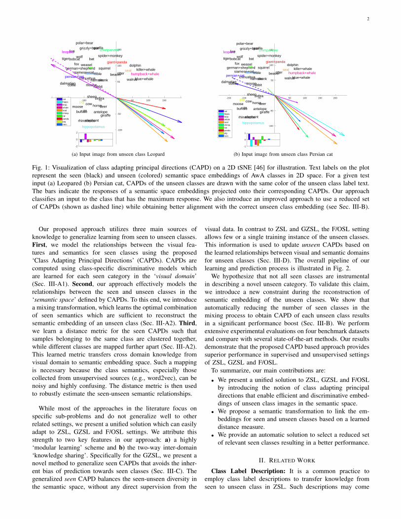
To provide a comprehensive and flexible solution to ZSL,GZSL and FSL problem settings, we introduce the conceptof principal directions that adapt to classes. In simple terms,CAPD is an embedding of the input image into the semanticspace such that, when projected onto CAPDs, the semanticspace embedding of the true class gives the highest response.A visualization of the CAPD concept is presented in Fig. 1. Asillustrated, the CAPDs of a Leopard (Fig. 1a) and a Persian catimage (Fig. 1b) point to their true semantic label embeddingshown in violet and blue respectively, which gives the highestprojection response in each case.
2
-150 -100 -50 50 100 150
-100
-50
50
100
150
antelope
grizzly+bear
killer+whalebeaver
dalmatian
horse
german+shepherd
blue+whale
siamese+cat
skunk
mole
tiger
moose
spider+monkey
elephant
gorilla
ox
fox
sheep
hamster
squirrel
rhinoceros
rabbit
bat
giraffe
wolf
chihuahua
weasel
otter
buffalo
zebra
deer
bobcat
lion
mouse
polar+bear
collie
walrus
cow
dolphin
persian+cat
hippopotamus
leopard
humpback+whaleseal
chimpanzee
rat
giant+panda
pig
raccoon
-2
0
2
cathippo.leop.whalesealchimp.ratpandapigracc.
(a) Input image from unseen class Leopard
-150 -100 -50 50 100 150 200
-150
-100
-50
50
100
150
antelope
grizzly+bear
killer+whalebeaver
dalmatian
horse
german+shepherd
blue+whale
siamese+cat
skunk
mole
tiger
moose
spider+monkey
elephant
gorilla
ox
fox
sheep
hamster
squirrel
rhinoceros
rabbit
bat
giraffe
wolf
chihuahua
weasel
otter
buffalo
zebra
deer
bobcat
lion
mouse
polar+bear
collie
walrus
cow
dolphin
persian+cat
hippopotamus
leopard
humpback+whaleseal
chimpanzee
rat
giant+panda
pig
raccoon
-1
0
1
cathippo.leop.whalesealchimp.ratpandapigracc.
(b) Input image from unseen class Persian cat
Fig. 1: Visualization of class adapting principal directions (CAPD) on a 2D tSNE [46] for illustration. Text labels on the plotrepresent the seen (black) and unseen (colored) semantic space embeddings of AwA classes in 2D space. For a given testinput (a) Leopared (b) Persian cat, CAPDs of the unseen classes are drawn with the same color of the unseen class label text.The bars indicate the responses of a semantic space embeddings projected onto their corresponding CAPDs. Our approachclassifies an input to the class that has the maximum response. We also introduce an improved approach to use a reduced setof CAPDs (shown as dashed line) while obtaining better alignment with the correct unseen class embedding (see Sec. III-B).
Our proposed approach utilizes three main sources ofknowledge to generalize learning from seen to unseen classes.First, we model the relationships between the visual fea-tures and semantics for seen classes using the proposed‘Class Adapting Principal Directions’ (CAPDs). CAPDs arecomputed using class-specific discriminative models whichare learned for each seen category in the ‘visual domain’(Sec. III-A1). Second, our approach effectively models therelationships between the seen and unseen classes in the‘semantic space’ defined by CAPDs. To this end, we introducea mixing transformation, which learns the optimal combinationof seen semantics which are sufficient to reconstruct thesemantic embedding of an unseen class (Sec. III-A2). Third,we learn a distance metric for the seen CAPDs such thatsamples belonging to the same class are clustered together,while different classes are mapped further apart (Sec. III-A2).This learned metric transfers cross domain knowledge fromvisual domain to semantic embedding space. Such a mappingis necessary because the class semantics, especially thosecollected from unsupervised sources (e.g., word2vec), can benoisy and highly confusing. The distance metric is then usedto robustly estimate the seen-unseen semantic relationships.
While most of the approaches in the literature focus onspecific sub-problems and do not generalize well to otherrelated settings, we present a unified solution which can easilyadapt to ZSL, GZSL and F/OSL settings. We attribute thisstrength to two key features in our approach: a) a highly‘modular learning’ scheme and b) the two-way inter-domain‘knowledge sharing’. Specifically for the GZSL, we present anovel method to generalize seen CAPDs that avoids the inher-ent bias of prediction towards seen classes (Sec. III-C). Thegeneralized seen CAPD balances the seen-unseen diversity inthe semantic space, without any direct supervision from the
visual data. In contrast to ZSL and GZSL, the F/OSL settingallows few or a single training instance of the unseen classes.This information is used to update unseen CAPDs based onthe learned relationships between visual and semantic domainsfor unseen classes (Sec. III-D). The overall pipeline of ourlearning and prediction process is illustrated in Fig. 2.
We hypothesize that not all seen classes are instrumentalin describing a novel unseen category. To validate this claim,we introduce a new constraint during the reconstruction ofsemantic embedding of the unseen classes. We show thatautomatically reducing the number of seen classes in themixing process to obtain CAPD of each unseen class resultsin a significant performance boost (Sec. III-B). We performextensive experimental evaluations on four benchmark datasetsand compare with several state-of-the-art methods. Our resultsdemonstrate that the proposed CAPD based approach providessuperior performance in supervised and unsupervised settingsof ZSL, GZSL and F/OSL.
To summarize, our main contributions are:• We present a unified solution to ZSL, GZSL and F/OSL
by introducing the notion of class adapting principaldirections that enable efficient and discriminative embed-dings of unseen class images in the semantic space.
• We propose a semantic transformation to link the em-beddings for seen and unseen classes based on a learneddistance measure.
• We provide an automatic solution to select a reduced setof relevant seen classes resulting in a better performance.
II. RELATED WORK
Class Label Description: It is a common practice toemploy class label descriptions to transfer knowledge fromseen to unseen class in ZSL. Such descriptions may come

3
from either supervised or unsupervised learning settings. Forthe supervised case, class attributes can be one source as well[12], [25], [35], [47]. These attributes are often generatedmanually, which is a laborious task. As a workaround, wordsemantic space embeddings derived from a large corpus ofunannotated text (e.g. from Wikipedia) can be used. Amongsuch unsupervised word semantic embeddings, word2vec [31],[30] and GloVe [36] vectors are frequently employed inZSL [58], [50]. These ZSL methods are sometimes (arguablyconfusingly) referred as unsupervised zero-shot learning [5],[1]. Supervised features tend to provide better performancethan the unsupervised ones. Nevertheless, unsupervised fea-tures provide more scalability and flexibility since they donot require expert annotation. Recent approaches attempt toadvance unsupervised ZSL by mapping textual representations(e.g. word2vec or GloVe) as attribute vectors using heuristicmeasures [23], [5]. In our work, we use both types of featuresand evaluate on both supervised and unsupervised ZSL todemonstrate the strength of our approach.
Embedding Space: ZSL strategies aim to map betweentwo different sources of information and two spaces: imageand label embeddings. Based on the mapping scheme, ZSLapproaches can be grouped into two categories. The firstcategory is attribute/word vector prediction. Given an image,they attempt to approximate label embedding and then classifyan unseen class image based on the similarity of predictedvector with unseen attribute/word vector. For example, inan early seminal work, [34] introduced a semantic outputcode classifier by using a knowledge base of attributes topredict unseen classes. [49], [26] proposed direct and indirectattribute prediction methods via a probabilistic realization. [55]formulated a discriminative model of category level attributes.[29] proposed an approach of transferring semantic knowl-edge from seen to unseen classes by a linear combinationof classifiers. The main problem with such direct attributeprediction is the poor performance when noisy or biasedattribute annotations are available. Jayaraman and Grauman[22] addressed this issue and proposed a discriminative modelfor ZSL.
Instead of predicting word vectors, the second category ofapproaches learn a compatibility function between image andlabel embeddings, which returns a compatibility score. Anunseen instance is then assigned to the class that gives themaximum score. For example, [2] proposed a label embeddingfunction that ranks correct class of unseen image higher thanincorrect classes. In [39], authors use the same principle but animproved loss function and regularizer. Qiao et al. [37] furtherimproved the former approach by incorporating a componentfor noise suppression. In a similar work, Xian et al. [50]added latent variables in the compatibility function whichcan learn a collection of label embeddings and select thecorrect embedding for prediction. Our method also has similarcompatibility function based on inner product of CAPD andcorresponding semantic vector. The use of CAPDs provide aneffective avenue to recognition.
Similarity Matching: This type of approaches build linearor nonlinear classifiers for each seen class, and then relatethose classifiers with unseen classes based on class-wise sim-
ilarity measures [7], [11], [18], [29], [38]. Our method findssimilar relation but instead of classifiers, we relate CAPDs ofseen and unseen classes. Moreover, we compute this relationon a learned metric of semantic embedding space which letus consider subtle discriminative details.
Few/One-shot Learning: FSL has a long history of investi-gation where few instances of some classes are used as labeledduring training [41], [13]. Although ZSL problem can easily beextended to FSL, established ZSL methods are not evaluated inFSL settings. A recent work [45] reports FSL performance ofonly two ZSL methods e.g. [43], [15]. In another work, [8],[19] presented FSL results on ImageNet. In this paper, weextend our approach to FSL settings and compare our methodwith the reported performance in [45].
Generalized Zero-shot Learning: GZSL setting signifi-cantly increases the complexity of the problem by allowingboth seen and unseen classes during testing phase [51], [9],[8]. This idea is related to open set recognition problem wheremethods consider to reject unseen objects in conjunction withrecognizing known objects [6], [21]. In open set case, methodsconsider all unseen objects as one outlier class. In contrast,GZSL represents unseen classes as individual separate cat-egories. Very few of the ZSL methods reported results onGZSL setting [8], [27], [52]. [15] proposed a joint visual-semantic embedding model to facilitate the generalization ofZSL. [43] offered a novelty detection mechanism which candetect whether the test image came from seen or unseencategory. Chao et al. [9] proposed a calibration mechanismto balance seen-unseen prediction score which any ZSL al-gorithm can adopt at decision making stage and proposed anevaluation method called Area Under Seen-Unseen accuracyCurve (AUSUC). Later, several other works [8], [52] adoptedthis evaluation strategy. In another recent work, Xian et al.[51] reported benchmarking results for both ZSL and GZSLperformance of several established methods published in theliterature. In this paper, we describe extension of our ZSLapproach to efficiently adapt with GZSL settings.
III. OUR APPROACH
Problem Formulation: Suppose, the set of all class labelsis y = y S ∪ y U where y S = {1, ...,S} and y U ={S+1, ...,S + U} are the sets of seen and unseen class labelsrespectively, with no overlap i.e., y S ∩ y U = ∅. Here, S andU denote the total number of seen and unseen classes, respec-tively. For all classes in the seen and unseen class sets, wehave associated semantic class embeddings (either attributesor word vectors) denoted by the sets ES = {es : s ∈ y S}and EU = {eu : u ∈ y U} respectively, where es, eu ∈ Rd.For every seen (s) and unseen (u) class, we have a numberof instances denoted by ns and nu respectively. The matricesXs = [x1
s, ...,xnss ] for s ∈ y S , and Xu = [x1
u, ...,xnuu ] for
u ∈ y U represent the image features for the seen class s andthe unseen class u, respectively, such that xs,xu ∈ Rk. Below,we define the three problem instances addressed in this paper:• Zero Shot Learning (ZSL): The image features of the
unseen classes Xu are not available during the trainingstage. The goal is to assign an unseen class label u ∈ y U
to a given unseen image using its feature vector xu.
4
13/10/2017 flow_new.xml
1/1
⟨ , ⟩pl vl
W1
WS
W2
⟨ , ⟩pu eu
.
.
.
. .
⟨ , ⟩pfu eu
W1
WU
W2 . . .
.
.
.
+
VGG orGoogleNet
x
γ
δ′
u
δu
pspgs
∈ ∪pl pu pgs
pfup
′
u
Projection
Projection
Projection
Few-shot case:
= arg ⟨ , ⟩y maxu
pfu eu
Conventional zero-shot case:
= arg ⟨ , ⟩y maxu
pu eu
Generalized zero-shot case:
= arg ⟨ , ⟩y maxl∈y
pl vl
∈ ∪vl es eu
UnseenClassifiers
SeenClassifiers
...
...
...
...
...
...
ZSL and GZSL Pipleline
FSL Pipleline
. .
α
pu
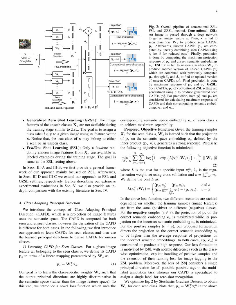
Fig. 2: Overall pipeline of conventional ZSL,FSL and GZSL method. Conventional ZSL:An image is passed through a deep networkto get an image feature x. Then, x is fed toseen classifiers Ws to produce seen CAPDs,ps. Afterwards, unseen CAPDs, pu are com-puted by linearly combining seen CAPDs usingα (or β for reduced case). Finally, predictionis done by computing the maximum projectionresponse of pu and unseen semantic embeddingseu. FSL: x is fed to unseen classifiers Wu toproduce another version of unseen CAPDs p′
u
which are combined with previously computedpu through δ′u and δu to find an updated versionof unseen CAPDs pf
u. Final prediction is doneby maximum response of pf
u and eu. GZSL:Seen CAPDs, ps of conventional ZSL setting aregeneralized using γ to produce generalized seenCAPDs, pg
s . For prediction, both pgs and pu are
considered for calculating maximum response ofCAPDs and their corresponding semantic embed-dings, es and eu.
• Generalized Zero Shot Learning (GZSL): The imagefeatures of the unseen classes Xu are not available duringthe training stage similar to ZSL. The goal is to assign aclass label l ∈ y to a given image using its feature vectorx. Notice that, the true class of x may belong to eithera seen or an unseen class.
• Few/One Shot Learning (FSL): Only a few/one ran-domly chosen image features from Xu are available aslabeled examples during the training stage. The goal issame as the ZSL setting above.
In Secs. III-A and III-B, we first provide a general frame-work of our approach mainly focused on ZSL. Afterwards,in Secs. III-D and III-C we extend our approach to FSL andGZSL settings, respectively. Before describing our extensiveexperimental evaluations in Sec. V, we also provide an in-depth comparison with the existing literature in Sec. IV.
A. Class Adapting Principal Direction
We introduce the concept of ‘Class Adapting PrincipalDirection’ (CAPD), which is a projection of image featuresonto the semantic space. The CAPD is computed for bothseen and unseen classes, however the derivation of the CAPDis different for both cases. In the following, we first introduceour approach to learn CAPDs for seen classes and then usethe learned principal directions to derive CAPDs for unseenclasses.
1) Learning CAPD for Seen Classes: For a given imagefeature xs belonging to the seen class s, we define its CAPDps in terms of a linear mapping parametrized by Ws as,
ps = WTs xs. (1)
Our goal is to learn the class-specific weights Ws such thatthe output principal directions are highly discriminative inthe semantic space (rather than the image feature space). Tothis end, we introduce a novel loss function which uses the
corresponding semantic space embedding es of seen class sto achieve maximum separability.
Proposed Objective Function: Given the training samplesXs for the seen class s, Ws is learned such that the projectionof ps on the semantic space embedding es, defined by theinner product 〈ps, es〉, generates a strong response. Precisely,the following objective function is minimized:
minWs
1
κ
S∑c=1
nc∑m=1
log(1 + exp
{L(xmc ;Ws)
})+λs2‖Ws ‖22
(2)where L is the cost for a specific input xmc , λs is the regu-larization weight set using cross validation and κ =
∑Sc=1 nc.
We define the cost L as:
L(xmc ;Ws) =
{〈ps, ec〉 − 〈ps, es〉, c 6= s〈ps, 1
S−1∑t 6=s
et〉 − 〈ps, es〉, c = s
In the above loss function, two different scenarios are tackleddepending on whether the training samples (image features)are from the same (positive) or different (negative) classes.For the negative samples (c 6= s), the projection of ps on thecorrect semantic embedding es is maximized while its pro-jection on the incorrect semantic embedding sc is minimized.For the positive samples (c = s), our proposed formulationdirects the projection on the correct semantic embedding esto be higher than the average response of projections onthe incorrect semantic embeddings. In both cases, 〈ps, es〉 isconstrained to produce a high response. Our loss formulationis motivated by [58], with notable differences such as the class-wise optimization, explicit handling of positive samples andthe extension of their ranking loss for image tagging to theZSL problem. Moreover, the loss of [58] considers a singleprincipal direction for all possible possible tags in the multi-label annotation task whereas our CAPD is specialized toassign a single label for zero-shot recognition.
We optimize Eq. 2 by Stochastic Gradient Descent to obtainWs for each seen class. Note that, ps = WT
s xmc in the above

5
ante
lope
dalm
atian
pers
ian+c
atho
rse
giraf
fe
chihu
ahua
zebr
aco
llie
AwA
0
0.5
1
1.5
2
2.5E
uclid
ean
dist
ance
similar-beforesimilar-afterdissimilar-beforedissimilar-after
Fig. 3: The effect of metric learning on semantic space withAwA attributes. The average Euclidean distances of top 5similar and dissimilar classes for example classes from AwAdataset are shown. The distances are illustrated for both withand without the application of metric learning. Metric learningbrings similar classes together while pulls dissimilar classesfurther apart.
cost function, thus for any sample xmc , ps changes when Ws isupdated at each training iteration. Also, the learning processof Ws for each seen class is independent of other classes.Therefore, all Ws can be learned jointly in a parallel fashion.Once the training process is complete, given an input visualfeature xmc , we generate one CAPD ps for each seen classusing Eq. 1. As a result, PS = [p1...pS] ∈ Rd×S accumulatesthe CAPDs of all the seen classes. Each CAPD is the mappedversion of the image feature on the class specific semanticspace. The CAPD vector and its corresponding semantic spaceembedding vector point to similar direction if the input featurebelongs to the same class.
2) Learning CAPD for Unseen Classes: In ZSL settings,the images of the unseen classes are not observed during thetraining. For this reason, we cannot directly learn a weightmatrix to calculate pu using the same approach as ps. Instead,for any unseen sample, we propose to approximate pu usingthe seen CAPD of the same sample. Here, we consider abilinear map, in particular, a linear combination of the seenclass CAPDs to generate the CAPD of the unseen class u:
pu =
S∑s=1
θs,ups = PSθu (3)
where, θu = [θ1,u...θS,u]T ∈ RS is the coefficient vector that,
in a way, aggregates the knowledge of seen classes into theunseen one. The computation of θu is subject to the relationbetween CAPDs and semantic embeddings of classes. Wedetail our approach to approximate θu below.
Metric Learning on CAPDs: The CAPDs reside in thesemantic embedding space. In this space, we learn a distancemetric to better model the similarities and dissimilaritiesamong the CAPDs. To this end, we assemble the sets of similarA and dissimilar A pairs of CAPDs that correspond to thepairs of training samples belonging to the same and differentseen classes, respectively. Our goal is to learn a distance metricdM such that the similar CAPDs are clustered together and the
dissimilar ones are mapped further apart. We minimize thefollowing objective which maximizes the squared distancesbetween the minimally separated dissimilar pairs:
maxM
min(i,j)∈A
d2M(pi,pj) s.t.∑
(i,j)∈A
d2M(pi,pj) ≤ 1 (4)
where dM =√(pi − pj)TM(pi − pj) is the Mahalanobis
distance metric [54]. After training, the most confusing dis-similar CAPD pairs are pulled apart while the similar CAPDsare clustered together by learning an optimal distance matrixM. Moreover, as metric learning is done on the semantic spaceit can help to measure the seen-unseen relation.
Our intuition is that, given a learning metric M in thesemantic embedding space, the relation between the semanticlabel embeddings of the seen es and the unseen classes euis analogous to that of their principal directions. Since thesemantic label embedding of unseen classes are available,we can estimate their relation with the seen classes. Forsimplicity, we consider a linear combination of semantic spaceembeddings:
eu =
S∑s=1
αs,ues = ESαu (5)
where, eu is the approximated semantic embedding ofeu corresponding to unseen class u. We compute αu =[α1,u...αS,u]
T ∈ RS by solving:
minαu
(eu − eu)TM(eu − eu) +
λu2‖ αu ‖22 (6)
where λu is a regularization parameter which is set via crossvalidation.
As we mentioned above, using the learned metric M, therelationship between the seen-unseen semantic embeddingsαu is analogous to the relationship between the seen-unseenCAPDs θu, thus θu ≈ αu. Here, M acts as a bridge betweenvisual features and their corresponding class semantics. Forexample, ‘giraffe’ is among top 5 close animals of ‘deer’in semantic space but after considering the metric M ‘cow’becomes closer than ‘giraffe’ because of its visual similaritywith deer. In Fig. 3, we highlight this behavior by calculatingaverage Euclidean distance (before and after applying M) oftop 5 similar and dissimilar classes. Essentially, metric learn-ing brings visually and semantically similar classes togetherwhile pulls dissimilar classes further apart. Accordingly, weapproximate the unseen CAPDs with seen CAPDs by rewritingEq. 3 as:
pu ≈ PSαu. (7)
We derive a CAPD, pu for each unseen class using Eq. 7. Intest stage of ZSL setting, we assign a given image feature xto an unseen class using the maximum projection response:
y = argmaxu〈pu, eu〉 (8)
6
far mid near randAwA
0
20
40
60
80
top-
1 ac
cura
cy
far mid near randCUB
0
10
20
30
40
top-
1 ac
cura
cy
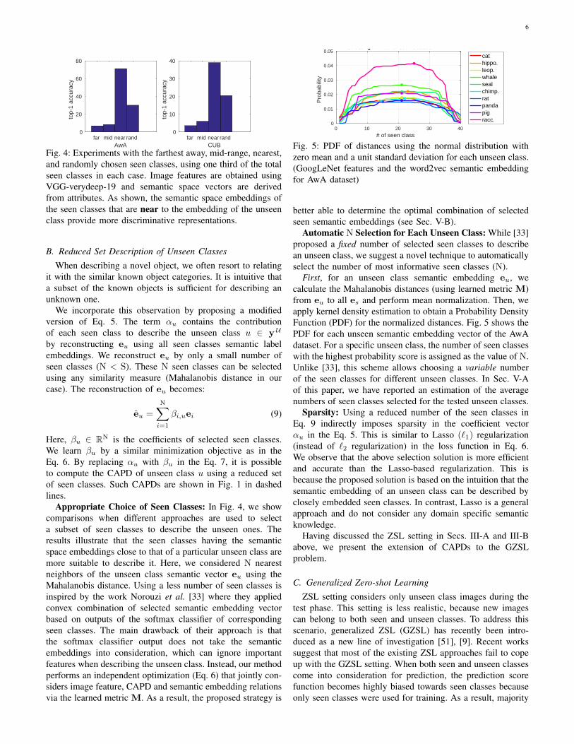
Fig. 4: Experiments with the farthest away, mid-range, nearest,and randomly chosen seen classes, using one third of the totalseen classes in each case. Image features are obtained usingVGG-verydeep-19 and semantic space vectors are derivedfrom attributes. As shown, the semantic space embeddings ofthe seen classes that are near to the embedding of the unseenclass provide more discriminative representations.
B. Reduced Set Description of Unseen Classes
When describing a novel object, we often resort to relatingit with the similar known object categories. It is intuitive thata subset of the known objects is sufficient for describing anunknown one.
We incorporate this observation by proposing a modifiedversion of Eq. 5. The term αu contains the contributionof each seen class to describe the unseen class u ∈ y U
by reconstructing eu using all seen classes semantic labelembeddings. We reconstruct eu by only a small number ofseen classes (N < S). These N seen classes can be selectedusing any similarity measure (Mahalanobis distance in ourcase). The reconstruction of eu becomes:
eu =
N∑i=1
βi,uei (9)
Here, βu ∈ RN is the coefficients of selected seen classes.We learn βu by a similar minimization objective as in theEq. 6. By replacing αu with βu in the Eq. 7, it is possibleto compute the CAPD of unseen class u using a reduced setof seen classes. Such CAPDs are shown in Fig. 1 in dashedlines.
Appropriate Choice of Seen Classes: In Fig. 4, we showcomparisons when different approaches are used to selecta subset of seen classes to describe the unseen ones. Theresults illustrate that the seen classes having the semanticspace embeddings close to that of a particular unseen class aremore suitable to describe it. Here, we considered N nearestneighbors of the unseen class semantic vector eu using theMahalanobis distance. Using a less number of seen classes isinspired by the work Norouzi et al. [33] where they appliedconvex combination of selected semantic embedding vectorbased on outputs of the softmax classifier of correspondingseen classes. The main drawback of their approach is thatthe softmax classifier output does not take the semanticembeddings into consideration, which can ignore importantfeatures when describing the unseen class. Instead, our methodperforms an independent optimization (Eq. 6) that jointly con-siders image feature, CAPD and semantic embedding relationsvia the learned metric M. As a result, the proposed strategy is
0 10 20 30 40
# of seen class
0
0.01
0.02
0.03
0.04
0.05
Pro
babi
lity
Selecting number of seen classes
cathippo.leop.whalesealchimp.ratpandapigracc.
Fig. 5: PDF of distances using the normal distribution withzero mean and a unit standard deviation for each unseen class.(GoogLeNet features and the word2vec semantic embeddingfor AwA dataset)
better able to determine the optimal combination of selectedseen semantic embeddings (see Sec. V-B).
Automatic N Selection for Each Unseen Class: While [33]proposed a fixed number of selected seen classes to describean unseen class, we suggest a novel technique to automaticallyselect the number of most informative seen classes (N).
First, for an unseen class semantic embedding eu, wecalculate the Mahalanobis distances (using learned metric M)from eu to all es and perform mean normalization. Then, weapply kernel density estimation to obtain a Probability DensityFunction (PDF) for the normalized distances. Fig. 5 shows thePDF for each unseen semantic embedding vector of the AwAdataset. For a specific unseen class, the number of seen classeswith the highest probability score is assigned as the value of N.Unlike [33], this scheme allows choosing a variable numberof the seen classes for different unseen classes. In Sec. V-Aof this paper, we have reported an estimation of the averagenumbers of seen classes selected for the tested unseen classes.
Sparsity: Using a reduced number of the seen classes inEq. 9 indirectly imposes sparsity in the coefficient vectorαu in the Eq. 5. This is similar to Lasso (`1) regularization(instead of `2 regularization) in the loss function in Eq. 6.We observe that the above selection solution is more efficientand accurate than the Lasso-based regularization. This isbecause the proposed solution is based on the intuition that thesemantic embedding of an unseen class can be described byclosely embedded seen classes. In contrast, Lasso is a generalapproach and do not consider any domain specific semanticknowledge.
Having discussed the ZSL setting in Secs. III-A and III-Babove, we present the extension of CAPDs to the GZSLproblem.
C. Generalized Zero-shot Learning
ZSL setting considers only unseen class images during thetest phase. This setting is less realistic, because new imagescan belong to both seen and unseen classes. To address thisscenario, generalized ZSL (GZSL) has recently been intro-duced as a new line of investigation [51], [9]. Recent workssuggest that most of the existing ZSL approaches fail to copeup with the GZSL setting. When both seen and unseen classescome into consideration for prediction, the prediction scorefunction becomes highly biased towards seen classes becauseonly seen classes were used for training. As a result, majority

7
of the unseen test instances are misclassified as seen examples.In other words, this bias notably decreases the classificationaccuracy on unseen classes while maintains relatively highaccuracy on seen classes. To solve this problem, availabletechniques attempts to estimate the prior probability of aninput belonging to either a seen or an unseen class [43], [9].However, this scheme heavily depends on the original datadistribution used for training.
Considering the above aspects, a competent GZSL methodshould possess the following properties:• Equilibrium: It should be able to balance seen-unseen
diversity so that the performances of both seen andunseen classes achieve a balance.
• Reduced data dependency: It should not receive anysupervision signal (obtained from either training or vali-dation set images) determining the likelihood of an inputbelonging to seen or unseen class.
• Consistency: It should retain its performance on theconventional ZSL setting as well.
In this work, we propose a novel GZSL algorithm to ade-quately address these challenges.
Generalized CAPD for Seen Class: In Sec. III-A, wedescribed the CAPD of seen classes for a given input imageis PS = [p1...pS]. Each seen CAPDs is obtained using theclass-wise learned classifier matrix Ws. It is obvious thateach Ws is biased to seen class ‘s’. For the same reason,each ps is also biased to class ‘s’. Since there was no seeninstance available during the testing phase in conventional ZSLsetting, seen CAPDs were not used for prediction (Eq. 8).Therefore, the inherent bias of seen CAPDs was not affectingZSL performance. In contrast, for GZSL settings, all seen andunseen CAPDs are considered for prediction. Thus, biasedseen CAPDs will dominate as expected and significantly affectthe unseen class performances. To solve this problem, wepropose to develop a generalized version of each seen CAPDas follows:
pgs = PSγs, (10)
where, γs denotes a parameter vector for seen class ‘s’.Proposed Objective Function: Our hypothesis is that the
bias towards seen classes that causes high scores duringprediction can be resolved using the semantic information ofclasses. To elaborate, γs is computed solely in semantic labelembedding domain and later applied to generalize CAPD ofseen class instances. We minimize the squared difference oftwo complementary losses to obtain γ = [γ1...γS] ∈ RS×S, as:
minγ‖
mean generalized seen loss︷ ︸︸ ︷1
S
S∑s=1
(ESγs − es)2−
mean unseen reconst. loss︷ ︸︸ ︷1
U
U∑u=1
(ESαu − eu)2 ‖22
+λγ2
S∑s=1
‖ γs ‖22, (11)
where λγ is the regularization weight set using cross valida-tion.
The objective function in Eq. 11 minimizes the squareddifference between the mean of two loss components. The first
component is the mean generalized seen loss which measuresthe reconstruction accuracy of seen class embedding es usingthe generalization parameters γs. The second component mea-sures the reconstruction accuracy of unseen class embeddingeu from seen classes. By reducing the squared differencebetween these two components, we indirectly balance thedistribution of seen-unseen diversity which effectively preventsthe domination of seen classes in the GZSL setting (the‘equilibrium’ property). The interesting fact is that our pro-posed generalization mechanism does not directly use CAPDs,yet it is strong enough to stabilize the CAPD of differentclasses during the prediction stage (the ‘less data dependence’property). Furthermore, the formulation does not affect thecomputation of unseen CAPDs i.e. pu which preserves theconventional ZSL performance (the ‘consistency’ property).
Prediction: For a given image feature x, we can derivegeneralized CAPDs of seen classes pgs and CAPD of unseenclasses pu using the description in Sec. III-B. In test stage,we consider both the projection responses of seen and unseenclasses to predict a class.
y = argmaxl∈y〈pl,vl〉 (12)
where, pl ∈ pu ∪ pgs and vl ∈ es ∪ eu.
D. Few-shot Learning
The few-shot learning (FSL) is a natural extension ofZSL. While ZSL considers no instance of an unseen classduring training, FSL relaxes this restriction by allowing a fewinstances of an unseen class as labeled during the trainingprocess. Another variant of FSL is called one-shot learning(OSL), which allows exactly one instance of an unseen class(instead of few) as labeled during training. An ideal ZSLapproach should be able to benefit from the labeled datafor unseen classes under F/OSL settings. In this section, weexplain how our approach is easily adaptable to FSL.
Updated CAPD for Unseen Class. In ZSL setting, fora given input image feature, we can calculate the unseenCAPD, pu for every unseen class ‘u’. Now, in the FSL setting,we optimally use the newly available labeled unseen datato update pu. To this end, new classifiers Wu are learnedfor each unseen class ‘u’ similar to the case of seen classes(Sec. III-A). For a given image feature, x, we can calculateunseen CAPDs by p′u = WT
ux. These CAPDs are fused withpu, which were derived from the linear combination of seenCAPDs (Eq. 7). The updated CAPD for unseen class ‘u’ isrepresented as pfu, given by:
pfu = δupu + δ′up′u, s.t. δu + δ′u = 1 (13)
where, δu and δ′u are the contribution of the respectiveCAPDs to form an updated CAPD of an unseen class. Duringprediction, we use pfu instead of pu in Eq. 8.
Calculation of δu and δ′u: The weights δu and δ′u are setusing training data such that they encode the reliability of puand p′u respectively. Recall that our prediction is based on thestrength of projection of a CAPD on the semantic embeddingvector. Therefore, we need to maximize the correspondence
8
between a CAPD and the correct semantic embedding vectori.e., a high 〈pu, eu〉. The unseen CAPD among pu and p′uthat provides higher projection response with uth unseen classsemantic vector gets a strong weight during the combinationin Eq. 13.
We derive pu and p′u for each training image feature,x ∈ XS = {Xs : s ∈ y S}, and the classification matrix ofunseen class ‘u’. Then, we find the summation of maximumprojection response of the CAPD (either pu or p′u) with itsrespective semantic vector. This maximum projection responsefinds the response of most similar (or confusing) unseen classof any image. The summation of this response across alltraining images can estimate the overall quality of CAPDsfrom the two sources. Finally, we normalize the summationsto get δu and δ′u as follows:
δu =
∑x∈XS maxu〈pu, eu〉∑
x∈XS maxu〈pu, eu〉+∑
x∈XS maxu〈p′u, eu〉,
δ′u =
∑x∈XS maxu〈p′u, eu〉∑
x∈XS maxu〈pu, eu〉+∑
x∈XS maxu〈p′u, eu〉.
(14)
In Fig. 9, we further elaborate the overall effect of δu and δ′uin FSL while using different semantic information.
E. Overall pipeline
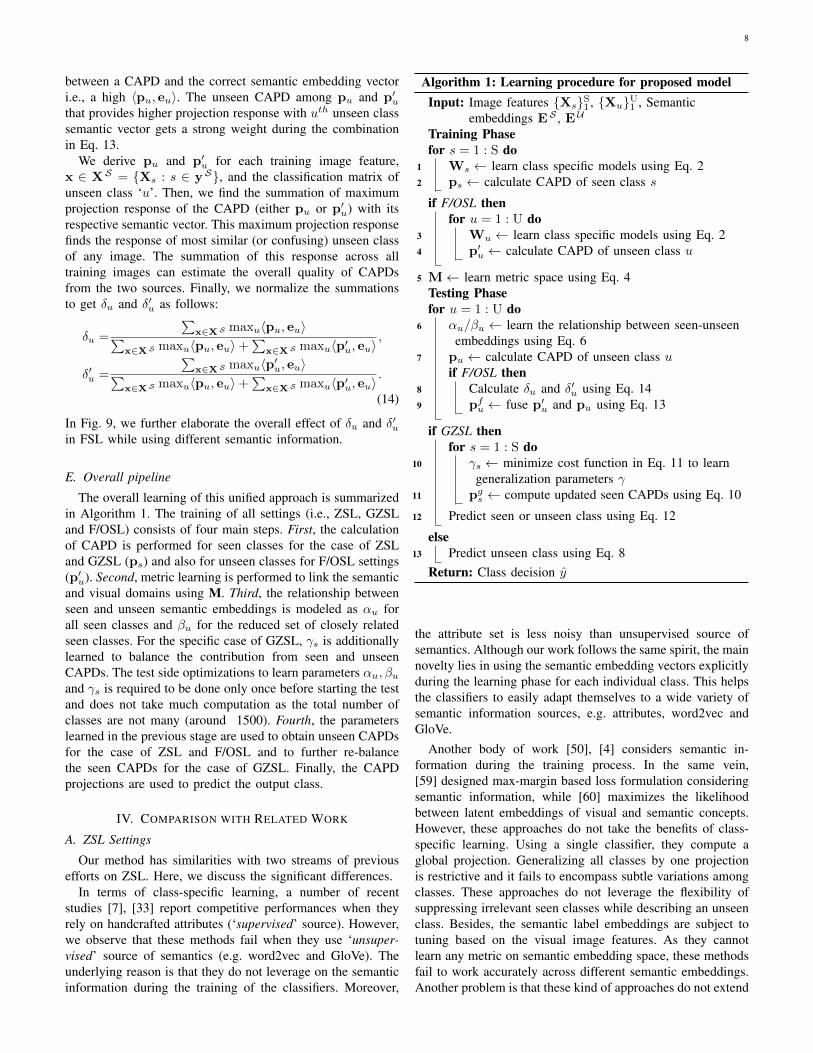
The overall learning of this unified approach is summarizedin Algorithm 1. The training of all settings (i.e., ZSL, GZSLand F/OSL) consists of four main steps. First, the calculationof CAPD is performed for seen classes for the case of ZSLand GZSL (ps) and also for unseen classes for F/OSL settings(p′u). Second, metric learning is performed to link the semanticand visual domains using M. Third, the relationship betweenseen and unseen semantic embeddings is modeled as αu forall seen classes and βu for the reduced set of closely relatedseen classes. For the specific case of GZSL, γs is additionallylearned to balance the contribution from seen and unseenCAPDs. The test side optimizations to learn parameters αu, βuand γs is required to be done only once before starting the testand does not take much computation as the total number ofclasses are not many (around 1500). Fourth, the parameterslearned in the previous stage are used to obtain unseen CAPDsfor the case of ZSL and F/OSL and to further re-balancethe seen CAPDs for the case of GZSL. Finally, the CAPDprojections are used to predict the output class.
IV. COMPARISON WITH RELATED WORK
A. ZSL Settings
Our method has similarities with two streams of previousefforts on ZSL. Here, we discuss the significant differences.
In terms of class-specific learning, a number of recentstudies [7], [33] report competitive performances when theyrely on handcrafted attributes (‘supervised’ source). However,we observe that these methods fail when they use ‘unsuper-vised’ source of semantics (e.g. word2vec and GloVe). Theunderlying reason is that they do not leverage on the semanticinformation during the training of the classifiers. Moreover,
Algorithm 1: Learning procedure for proposed modelInput: Image features {Xs}S1 , {Xu}U1 , Semantic
embeddings ES , EU
Training Phasefor s = 1 : S do
1 Ws ← learn class specific models using Eq. 22 ps ← calculate CAPD of seen class s
if F/OSL thenfor u = 1 : U do
3 Wu ← learn class specific models using Eq. 24 p′u ← calculate CAPD of unseen class u
5 M← learn metric space using Eq. 4Testing Phasefor u = 1 : U do
6 αu/βu ← learn the relationship between seen-unseenembeddings using Eq. 6
7 pu ← calculate CAPD of unseen class uif F/OSL then
8 Calculate δu and δ′u using Eq. 149 pfu ← fuse p′u and pu using Eq. 13
if GZSL thenfor s = 1 : S do
10 γs ← minimize cost function in Eq. 11 to learngeneralization parameters γ
11 pgs ← compute updated seen CAPDs using Eq. 10
12 Predict seen or unseen class using Eq. 12
else13 Predict unseen class using Eq. 8
Return: Class decision y
the attribute set is less noisy than unsupervised source ofsemantics. Although our work follows the same spirit, the mainnovelty lies in using the semantic embedding vectors explicitlyduring the learning phase for each individual class. This helpsthe classifiers to easily adapt themselves to a wide variety ofsemantic information sources, e.g. attributes, word2vec andGloVe.
Another body of work [50], [4] considers semantic in-formation during the training process. In the same vein,[59] designed max-margin based loss formulation consideringsemantic information, while [60] maximizes the likelihoodbetween latent embeddings of visual and semantic concepts.However, these approaches do not take the benefits of class-specific learning. Using a single classifier, they compute aglobal projection. Generalizing all classes by one projectionis restrictive and it fails to encompass subtle variations amongclasses. These approaches do not leverage the flexibility ofsuppressing irrelevant seen classes while describing an unseenclass. Besides, the semantic label embeddings are subject totuning based on the visual image features. As they cannotlearn any metric on semantic embedding space, these methodsfail to work accurately across different semantic embeddings.Another problem is that these kind of approaches do not extend

9
well for generalized zero-shot and few shot scenario becausethe training easily gets biased to seen classes which makesdifficult to generalize [51] and cannot utilize newly availabletest data in few-shot settings. In contrast, by taking the benefitsof class-specific learning, our approach computes CAPD foreach classifier that can significantly enhance the learned dis-criminative information. In addition, our approach describesthe unseen class with automatically selected informative seenclasses and learns a metric on the semantic embedding spaceto further fine-tune the semantic label information. Moreover,our approach can work simultaneously in GZSL and O/FSLsettings.
In terms of relating seen and unseen by a linear combinationour method has similarity with some previous efforts [48],[56], [5], [10]. [48], [56] applied the combination to convertZSL problem to a supervised learning problem by generatingvirtual or synthesized data. For doing so, these approachesrequired the names of unseen classes during training timewhich makes unseen pre-defined. [5], [10] used combinationof both attribute vector and word vector together in trainingto relate seen and unseen in semantic space. However, theseapproaches do not require attribute vectors during testing. Itreduces the costly annotation of unseen classes in testing butstill utilize costly manual labeling of attributes of seen classesduring training. In contrast, our method utilize the seen-unseencombination in an unique way to solve ZSL, GZSL and O/FSLproblem. We do not use the concept of attributes to improvethe performance of word vectors. Therefore, the unsupervisedversion of our work is not depended on strong supervisionduring training.
Many traditional methods focus ZSL but do not performwell in GZSL (See Table VIII, IX and X). Some othermethods need to modify ZSL to trusductive [27] or domainadaptation [52] settings to achieve generalization. Again, manyapproaches perform FSL but do not have the extendibility tozero-shot settings [41], [13]. Moreover, some approaches seemto overfit on small scale dataset, specific image features, andspecific semantic vector i.e. supervised-attributes ([59], [60])or unsupervised word2vec/Glove ([4], [50]). Our method, onthe other hand, consistently provides improved performanceacross all the different semantic information and problemsettings.
B. GZSL settings
We automatically balance the diversity of seen-unseenclasses in an unsupervised way, without strongly relying onCAPD or image visual feature. Previous efforts used a su-pervision mechanism either from training or validation imagedata to determine if any input image belongs to a seen oran unseen class. Chao et al. [9] proposed a calibration basedapproach to rescale the seen scores and evaluated using AreaUnder Seen-Unseen accuracy Curve (AUSUC) [7], [52]. Asprediction scores of GZSL are strongly biased to seen classes,they proposed to calibrate seen scores by adding a constantnegative bias termed as a calibration factor. This factor iscalculated on a validation set and works as a prior likelihood ofa data point being from a seen/unseen class. The drawback of
such an approach is that it acts as a post-processing mechanismapplied at the decision making stage, not dealing with thegeneralization at the basic algorithmic level.
Another alternative work, CMT method [43] incorporatesa novelty detection approach which estimates the outlierprobability of an input image. Again, the outlier probabilityis determined using training images which provides an extraimage-based supervision to GZSL model. In contrary, ourmethod considers the seen-unseen biasness in the semanticspace at the algorithmic level. The overall prediction scoresare then balanced to remove the inherent biasness towards theseen classes. We show that such an approach can be useful forboth supervised attributes and unsupervised word2vec/GloVeas semantic embedding information. As our approach doesnot follow the post-processing strategy like [9], [7], [52],we do not evaluate our work with AUSUC. In line withthe recommendation in [50], we use harmonic mean basedapproach for GZSL evaluation.
V. EXPERIMENTS
Benchmark Datasets: We use four standard datasets forour experiments; aPascal & aYahoo (aPY) [12], Animalswith Attributes (AwA) [25], SUN attributes (SUN) [35], andCaltech-UCSD Birds (CUB) [47]. The statistics of thesedatasets are given in Table I. We follow the standard protocols(seen/unseen splits of classes) used in the literature. To bespecific, we have exactly followed [50] for AwA and CUBdatasets, [59], [60] for aPY and SUN-10 and [7] for SUN. Toincrease the complexity of GZSL task for SUN, we used adifferent of seen/unseen split introduced in [7]. In line withthe standard protocol, the test images correspond to onlyunseen classes in ZSL settings. In Few/One-shot settings, werandomly choose three/one instances per unseen class to use intraining as labeled examples. Again, in GZSL settings, we per-form a 80-20% split of each seen class instances; 80% portionis used in training and rest 20% for testing in conjunction withall unseen test data. We report the average results of 10 randomtrails for Few/One shot or GZSL settings. In a recent work,Xian et al. [51] proposed a different seen/unseen split for theabove mentioned four datasets. We perform GZSL experimentson that setting as well. We conduct large scale experiment forZSL problem on ImageNet (ILSVRC) 2012/2010 dataset withthe setting of [16], [57]. The training and testing are done onthe images of 1K class of ILSVRC 2012 and non-overlapped360 classes of ILSVRC 2010 dataset respectively. It makes1.2M images in training from ILSVRC 2012 and 54K imagesfrom ILSVRC 2010.
Image Features: Previous ZSL approaches use both shal-low (SIFT, PHOG, Fisher Vector, color histogram) and deepfeatures [4], [7], [37]. As reported repeatedly, deep featuresoutperform shallow features by a significant margin [7]. Forthis reason, we consider only deep features from the pretrainedGoogLeNet [44] and VGG-verydeep-19 [42] models for ourcomparisons. For feature extraction from GoogLeNet andVGG-verydeep-19, we exactly follow Changpinyo et al. [7]and Zhang et al. [59], respectively. The dimension of vi-sual features extracted from GoogLeNet is 1024, and VGG-verydeep-19 is 4096. While using the recent Xian et al. [51]
10
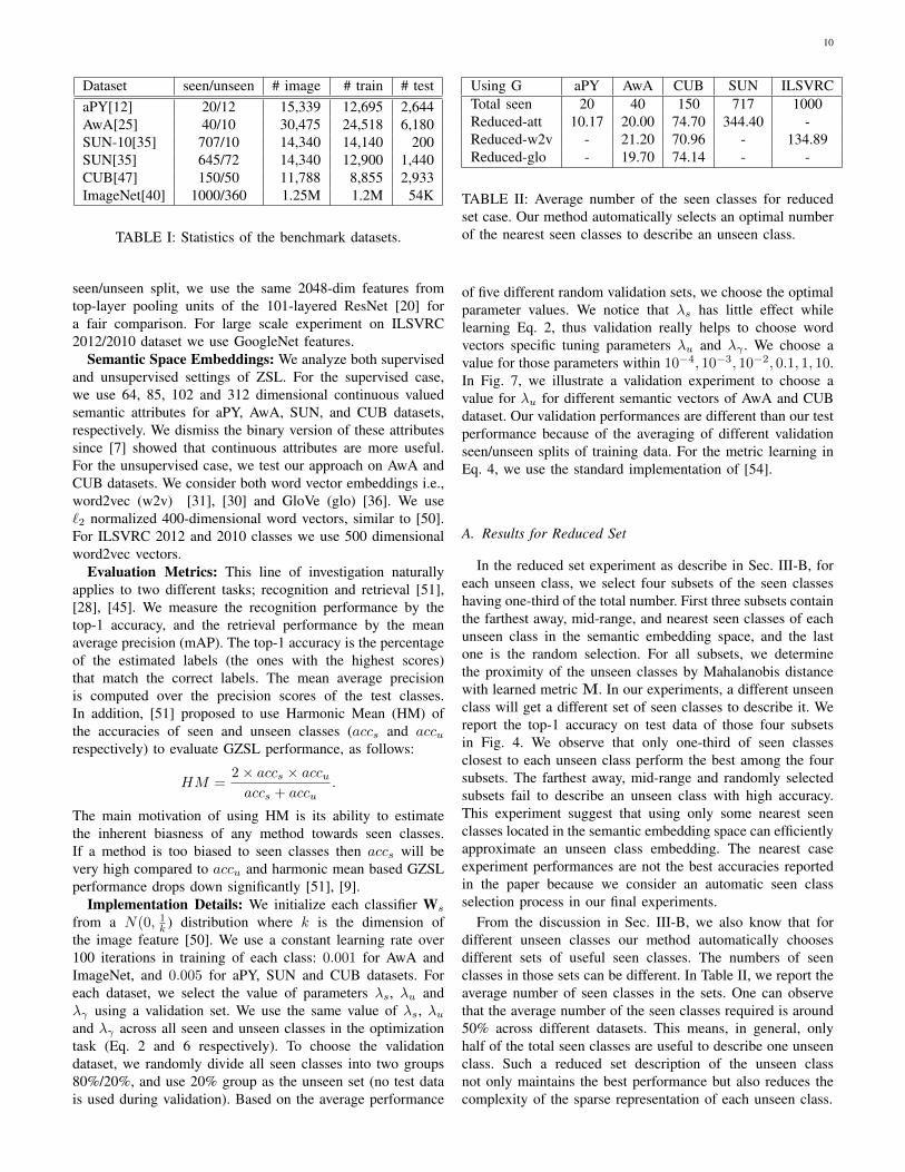
Dataset seen/unseen # image # train # testaPY[12] 20/12 15,339 12,695 2,644AwA[25] 40/10 30,475 24,518 6,180SUN-10[35] 707/10 14,340 14,140 200SUN[35] 645/72 14,340 12,900 1,440CUB[47] 150/50 11,788 8,855 2,933ImageNet[40] 1000/360 1.25M 1.2M 54K
TABLE I: Statistics of the benchmark datasets.
seen/unseen split, we use the same 2048-dim features fromtop-layer pooling units of the 101-layered ResNet [20] fora fair comparison. For large scale experiment on ILSVRC2012/2010 dataset we use GoogleNet features.
Semantic Space Embeddings: We analyze both supervisedand unsupervised settings of ZSL. For the supervised case,we use 64, 85, 102 and 312 dimensional continuous valuedsemantic attributes for aPY, AwA, SUN, and CUB datasets,respectively. We dismiss the binary version of these attributessince [7] showed that continuous attributes are more useful.For the unsupervised case, we test our approach on AwA andCUB datasets. We consider both word vector embeddings i.e.,word2vec (w2v) [31], [30] and GloVe (glo) [36]. We use`2 normalized 400-dimensional word vectors, similar to [50].For ILSVRC 2012 and 2010 classes we use 500 dimensionalword2vec vectors.
Evaluation Metrics: This line of investigation naturallyapplies to two different tasks; recognition and retrieval [51],[28], [45]. We measure the recognition performance by thetop-1 accuracy, and the retrieval performance by the meanaverage precision (mAP). The top-1 accuracy is the percentageof the estimated labels (the ones with the highest scores)that match the correct labels. The mean average precisionis computed over the precision scores of the test classes.In addition, [51] proposed to use Harmonic Mean (HM) ofthe accuracies of seen and unseen classes (accs and accurespectively) to evaluate GZSL performance, as follows:
HM =2× accs × accuaccs + accu
.
The main motivation of using HM is its ability to estimatethe inherent biasness of any method towards seen classes.If a method is too biased to seen classes then accs will bevery high compared to accu and harmonic mean based GZSLperformance drops down significantly [51], [9].
Implementation Details: We initialize each classifier Ws
from a N(0, 1k ) distribution where k is the dimension ofthe image feature [50]. We use a constant learning rate over100 iterations in training of each class: 0.001 for AwA andImageNet, and 0.005 for aPY, SUN and CUB datasets. Foreach dataset, we select the value of parameters λs, λu andλγ using a validation set. We use the same value of λs, λuand λγ across all seen and unseen classes in the optimizationtask (Eq. 2 and 6 respectively). To choose the validationdataset, we randomly divide all seen classes into two groups80%/20%, and use 20% group as the unseen set (no test datais used during validation). Based on the average performance
Using G aPY AwA CUB SUN ILSVRCTotal seen 20 40 150 717 1000Reduced-att 10.17 20.00 74.70 344.40 -Reduced-w2v - 21.20 70.96 - 134.89Reduced-glo - 19.70 74.14 - -
TABLE II: Average number of the seen classes for reducedset case. Our method automatically selects an optimal numberof the nearest seen classes to describe an unseen class.
of five different random validation sets, we choose the optimalparameter values. We notice that λs has little effect whilelearning Eq. 2, thus validation really helps to choose wordvectors specific tuning parameters λu and λγ . We choose avalue for those parameters within 10−4, 10−3, 10−2, 0.1, 1, 10.In Fig. 7, we illustrate a validation experiment to choose avalue for λu for different semantic vectors of AwA and CUBdataset. Our validation performances are different than our testperformance because of the averaging of different validationseen/unseen splits of training data. For the metric learning inEq. 4, we use the standard implementation of [54].
A. Results for Reduced Set
In the reduced set experiment as describe in Sec. III-B, foreach unseen class, we select four subsets of the seen classeshaving one-third of the total number. First three subsets containthe farthest away, mid-range, and nearest seen classes of eachunseen class in the semantic embedding space, and the lastone is the random selection. For all subsets, we determinethe proximity of the unseen classes by Mahalanobis distancewith learned metric M. In our experiments, a different unseenclass will get a different set of seen classes to describe it. Wereport the top-1 accuracy on test data of those four subsetsin Fig. 4. We observe that only one-third of seen classesclosest to each unseen class perform the best among the foursubsets. The farthest away, mid-range and randomly selectedsubsets fail to describe an unseen class with high accuracy.This experiment suggest that using only some nearest seenclasses located in the semantic embedding space can efficientlyapproximate an unseen class embedding. The nearest caseexperiment performances are not the best accuracies reportedin the paper because we consider an automatic seen classselection process in our final experiments.
From the discussion in Sec. III-B, we also know that fordifferent unseen classes our method automatically choosesdifferent sets of useful seen classes. The numbers of seenclasses in those sets can be different. In Table II, we report theaverage number of seen classes in the sets. One can observethat the average number of the seen classes required is around50% across different datasets. This means, in general, onlyhalf of the total seen classes are useful to describe one unseenclass. Such a reduced set description of the unseen classnot only maintains the best performance but also reduces thecomplexity of the sparse representation of each unseen class.

11
Method aPY AwA SUN CUBV G V G V G V G
Ours [all-seen] 45.84 50.64 73.19 64.74 84.5 87.00 39.86 42.31Ours [reduced-Lasso] 36.54 37.22 74.16 75.76 78.50 84.50 37.47 37.37Ours [reduced-auto w/o M] 46.90 42.78 76.42 77.51 85.00 89.50 42.34 41.36Ours [reduced-auto with M] 54.69 55.07 78.53 80.43 85.00 79.00 43.01 45.31
TABLE III: Top-1accuracy (in %) ofvarious versions ofCAPD using attributes.V: VGG-verydeep-19,G: GoogLeNet features.
Our approach
629
519
587
708
346
669
241
680
165
427
cat
hipp
o.
leop
.
wha
le
seal
chim
p. rat
pand
a
pig
racc
.
cat
hippo.
leop.
whale
seal
chimp.
rat
panda
pig
racc.
0
100
200
300
400
500
600
700latEm
677
433
581
392
138
390
703
287
253
385
cat
hipp
o.
leop
.
wha
le
seal
chim
p. rat
pand
a
pig
racc
.cat
hippo.
leop.
whale
seal
chimp.
rat
panda
pig
racc.
0
100
200
300
400
500
600
700
Fig. 6: Confusion matrices on AwA dataset using GoogLeNetas image features and the attributes as semantic space vectors.Left: Xian et al. [50]. Right: CAPD. As seen, CAPD providebetter overall and class-wise performance.
AwA
att w2v glove0
20
40
60
80
acc
(%)
CUB
att w2v glove0
10
20
30
40
acc
(%)
.0001 .001 .01 .1 1 10
Fig. 7: Validation experiment for choosing λu
B. Benchmark Comparisons
We discuss benchmark performances of ZSL recognitionand retrieval for both supervised (attributes) and unsupervisedsemantics (word2vec or GloVe).
1) Results for ZSL with Supervised Attributes1: We presentthe top-1 ZSL accuracy results of different versions of ourmethod in Table III. In the all-seen case, we have consideredall seen classes to describe an unseen class (Eq. 5). In Lasso,we report the performance using Lasso regularization in placeof `2 in Eq. 6. The results demonstrate that using a reducednumber of seen classes with (M 6= I) or without (M = I)metric learning to describe an individual unseen class canimprove ZSL accuracy. Performance with the metric learningoutperforms all other variations of the method in almostevery cases except SUN dataset because the implementationof metric learning uses same number images per class foreach dataset. However, SUN has a large number of classesbut contains less number of images per class. In Table IV,we compare the overall top-1 accuracy of our method (after
1For fairness, inductive test performances from DSRL [53], MFMR [52]and DMaP [27] are reported in the tables.
Using V aPY AwA SUN CUBLampert’14 [26] 38.16 57.23 72.00 31.40ESZSL’15 [39] 24.22 75.32 82.10 -SSE-ReLU’15 [59] 46.23 76.33 82.50 30.41Zhang’16 [60] 50.35 80.46 83.30 42.11Bucher’16 [28] 53.15 77.32 84.41 43.29DSRL’17[53] 56.29 77.38 82.00 50.26MFMR’17[52] 48.20 79.80 84.00 47.70Ours 54.69 78.53 85.00 43.33Using G aPY AwA SUN CUBLampert’14 [26] 37.10 59.50 - -Akata’15 [4] - 66.70 - 50.10Changpinyo’16 [7] - 72.90 - 45.85Xian’16 [50] - 72.50 - 45.60SCoRe’17[32] - 78.30 - 58.40MFMR’17[52] 46.40 76.60 81.50 46.20EXEM’17[8] - 77.20 - 59.80Ours 55.07 80.83 87.00 45.31
TABLE IV: Supervised ZSL top-1 accuracy (in %) on fourstandard datasets. V: VGG-verydeep-19 and G: GoogLeNetimage features. Results are from the original papers. Only veryrecent SOTA methods are considered for comparison.
Using V aPY AwA SUN CUBSSE-INT’15 [59] 15.43 46.25 58.94 4.69SSE-ReLU’15 [59] 14.09 42.60 44.55 3.70Bucher’16 [28] 36.92 68.10 52.68 25.33Zhang’16 [60] 38.30 67.66 80.10 29.15MFMR’17 [52] 45.60 70.80 77.40 30.60Ours 43.85 72.87 80.20 36.60
TABLE V: Supervised ZSL retrieval performance (in mAP).V: VGG-verydeep-19 image features.
using validated parameter settings) with many recent ZSLapproaches. Our approach outperforms other methods in mostof the settings. In Fig. 6, we show confusion matrices of arecent approach [50] and ours. Similar to recognition, ZSLcan also perform retrieval task. ZSL retrieval is to searchimages of unseen classes using their class label embeddings.We test the attributes set as a query to retrieve test images. InTable V, we compare our ZSL retrieval performance with fourrecent approaches on four datasets. Our approach performsconsistently better or comparable to state-of-the-art methods.
2) Results for ZSL with Unsupervised Semantics: ZSL withpretrained word vectors [31], [36] as sematnic embedding isthe focus of attention nowadays since it is difficult to generatemanually annotated attribute sets in real-world applications.
12
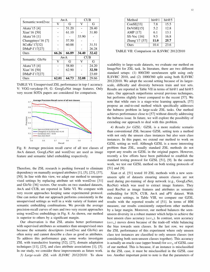
Semantic:word2vec AwA CUBV G V G
Akata’15 [4] - 51.20 - 28.40Xian’16 [50] - 61.10 - 31.80Akata’16 [1] - - 33.90 -Changpinyo’16 [7] - 57.50 - -SCoRe’17[32] - 60.88 - 31.51DMaP-I’17[27] - - - 26.28Ours 66.26 66.89 34.40 32.42
Semantic: GloVe AwA CUBV G V G
Akata’15 [4] - 58.80 - 24.20Xian’16 [50] - 62.90 - 32.50DMaP-I’17[27] - - - 23.69Ours 62.01 64.73 32.08 29.66
TABLE VI: Unsupervised ZSL performance in top-1 accuracy.V: VGG-verydeep-19, G: GoogLeNet image features. Onlyvery recent SOTA papers are considered for comparison.
0.5 0.6 0.7 0.8 0.9 1
Recall
0
0.1
0.2
0.3
0.4
0.5
0.6
0.7
Pre
cisi
on
Average Precision-Recall curve of all test classes
Xian et al.(2016) AUC=47.06Changpinyo et al.(2016) AUC=41.40Ours(lasso) AUC = 53.92Ours AUC=55.97
Fig. 8: Average precision recall curve of all test classes ofAwA dataset. GoogLeNet and word2vec are used as imagefeature and semantic label embedding respectively.
Therefore, the ZSL research is pushing forward to eliminatedependency on manually assigned attributes [1], [5], [23], [37],[50]. In line with this view, we adapt our method to unsuper-vised settings by replacing attribute set with word2vec [31]and GloVe [36] vectors. Our results on two standard datasets,AwA and CUB, are reported in Table VI. We compare withvery recent approaches keeping same experimental protocol.One can notice that our approach performs consistently in theunsupervised settings as well in a wide variety of feature andsemantic embedding combinations. We provide the averageprecision-recall curves of ours and two very recent approachesusing word2vec embeddings in Fig. 8. As shown, our methodis superior to others by a significant margin.
Our observation is that ZSL attains better performancewith supervised attributes as semantics than unsupervised onesbecause the semantic descriptors (word2vec and GloVe) areoften noisy and cannot describe a class as good as attributes.To address this performance gap, some works investigateZSL with transductive learning [52], [27], domain adaptationtechniques [11], [23], and class attribute associations [1], [5].In our study, we consider these improvements as future work.
3) Large-scale ZSL with ILSVRC 2012/2010: To show
Method hit@1 hit@5ConSE[33] 7.8 15.5DeViSE[15] 5.2 12.8AMP [17] 6.1 13.1SS-Voc [16] 9.5 16.8Zhang’17 [57] 11.0 25.7Ours 10.4 23.6
TABLE VII: Comparison on ILSVRC 2012/2010
scalability to large-scale datasets, we evaluate our method onImageNet for ZSL task. In literature, there are two differentstandard setups: (1) 800/200 seen/unseen split using onlyILSVRC 2010, and (2) 1000/360 split using both ILSVRC2012/2010. We adopt the second setting because of its larger-scale, difficulty and diversity between train and test sets.Results are reported in Table VII in terms of hit@1 and hit@5rates. Our approach outperforms several previous techniques,but performs slightly lower compared to the recent [57]. Wenote that while ours is a stage-wise learning approach, [57]propose an end-to-end method which specifically addressesthe hubness problem in large-scale ZSL tasks. Our methodachieves performance close to [57] without directly addressingthe hubness issue. In future, we will explore the possibility ofextending our approach to deal with this problem.
4) Results for GZSL: GZSL is a more realistic scenariothan conventional ZSL because GZSL setting tests a methodwith not only the unseen class instances but also seen classinstances. In this paper, we extend our method to work onGZSL setting as well. Although GZSL is a more interestingproblem than ZSL, usually standard ZSL methods do notreport any results on GZSL in the original papers. However,recently a few efforts have been published to establish thestandard testing protocol for GZSL [51], [9]. In the currentwork, we test our GZSL method on both testing protocols of[51] and [9].
Xian et al. [51] tested 10 ZSL methods with a new seen-unseen split of datasets ensuring unseen classes are notused during pre-training of deep network (e.g., GoogLeNet,ResNet) which was used to extract image features. Theyused ResNet as image features and attributes as semanticembedding for SUN, CUB, AwA and aPY dataset. Withthis exact settings, in Table VIII, we compare our GZSLresults with the reported results of [51]. In terms of HMmeasure, our results consistently outperform other methodsby a large margin. Moreover, our method balances the seen-unseen diversity in a robust manner which helps to achieve thebest unseen class accuracy (accu). In contrast, seen accuracy(accu) moves down because of the trade-off while balancingthe bias towards seen classes. In the last row, we reportthe ZSL performance of this experiment where only unseenclass test instances are classified to only unseen classes (notconsidering both seen-unseen classes together). This accuracyis actually an oracle case (upper bound) for accu of GZSL caseof our method. This is because, if an instance is misclassifiedin the ZSL case, it must be misclassified in the GZSL casetoo. Another important point to note is that the parameters of

13
Top1 SUN CUB AWA aPYResNet HM accs accu HM accs accu HM accs accu HM accs accuDAP[26] 7.2 25.1 4.2 3.3 67.9 1.7 0.0 88.7 0.0 9.0 78.3 4.8CONSE[33] 11.6 39.9 6.8 3.1 72.2 1.6 0.8 88.6 0.4 0.0 91.2 0.0CMT[43] 13.3 28.0 8.7 8.7 60.1 4.7 15.3 86.9 8.4 19.0 74.2 10.9SSE[59] 4.0 36.4 2.1 14.4 46.9 8.5 12.9 80.5 7.0 0.4 78.9 0.2LATEM[50] 19.5 28.8 14.7 24.0 57.3 15.2 13.3 71.7 7.3 0.2 73.0 0.1ALE[3] 26.3 33.1 21.8 34.4 62.8 23.7 27.5 76.1 16.8 8.7 73.7 4.6DEVISE[15] 20.9 27.4 16.9 32.8 53.0 23.8 22.4 68.7 13.4 9.2 76.9 4.9SJE[4] 19.8 30.5 14.7 33.6 59.2 23.5 19.6 74.6 11.3 6.9 55.7 3.7ESZSL[39] 15.8 27.9 11.0 21.0 63.8 12.6 12.1 75.6 6.6 4.6 70.1 2.4SYNC[7] 13.4 43.3 7.9 19.8 70.9 11.5 16.2 87.3 8.9 13.3 66.6 7.4Our GZSL 31.3 27.8 35.8 43.3 41.7 44.9 54.5 68.6 45.2 37.0 59.5 26.8Our ZSL 49.7 53.8 52.6 39.3
TABLE VIII: GZSL performance comparison with other established methods in the literature. The experiment setting is exactlysame as in [51]. Image features are taken from ResNet and attributes are used as semantic information.
Top1:G AwA CUBHM accs accu HM accs accu
DAP[26] 4.7 77.9 2.4 7.5 55.1 4.0IAP[26] 3.3 76.8 1.7 2.0 69.4 1.0ConSE[33] 16.9 75.9 9.5 3.5 69.9 1.8SynC[7] 0.8 81.0 0.4 22.3 72.0 13.2MFMR[52] 29.60 75.6 18.4 - - -Our GZSL 50.8 43.2 61.7 29.5 23.4 39.9Our ZSL 76.2 44.0
TABLE IX: GZSL performance comparison with the experi-ment settings of [9]. Image features are taken from GoogLeNetand attributes are used as semantic information.
Top1:Mean AwA CUBatt w2v att glo
DMaP[27] 17.23 6.44 13.55 2.07Our GZSL 52.45 43.70 31.65 18.75
TABLE X: Comparison with a recent GZSL work DMaP[27]
our method are tuned for GZSL setting in this experiment.Therefore, ZSL performance in the last row may increase ifone tunes parameters for the ZSL setting.
Chao et al. [9] experimented GZSL with standard seen-unseen split used in ZSL literature. Keeping this split, theykept random 80% seen class images for training and heldout the rest of 20% images for testing stage during GZSL.We perform the same harmonic mean based evaluation likeprevious setting. In Table IX, we compare our results withthe reported results in [9]. Using the same settings, we alsocompare with two recent methods, MFMR [52] (Table IX)and DMAP [27] (Table X). For the sake of comparison withDMAP [27], we compare mean Top1 accuracy (not standardthough) instead of harmonic mean because accu and accsare not reported separately in the [27]. Again, our methodperforms consistently well across datasets. More results onGZSL for AwA, CUB, SUN and aPY datasets are reported inTable XII.
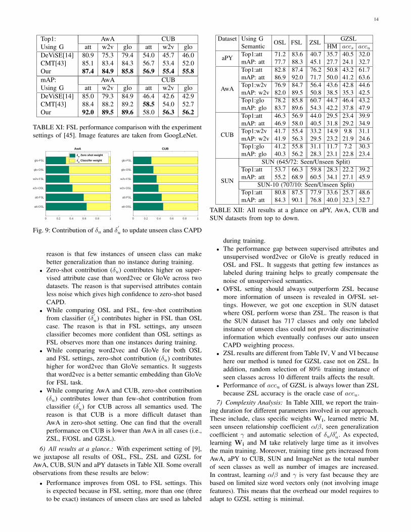
5) Results for FSL: As stated earlier, our method can easilytake the advantage when new unseen class instances becomeavailable as labeled data for training. To test this scenario, inFSL settings, we assume three instances of each unseen class(randomly chosen) are available as labeled during training.In Table XI, we report our results for FSL on AwA andCUB dataset while using attribute, word2vec and GloVe assemantic information. The compared methods, DeViSE [14]and CMT[43], did not report FSL performance in the originalpaper. But, [45] reimplemented the original work to adapt FSL.The exact three instances of each unseen class used in [45]are not publically available. However, to make our resultscomparable with others, we report the average performanceof 10 random trails. Our method performs consistently betterthan comparing methods except one case: mAP of CUB-att (58.0 vs 58.5). Another observation from these resultsis that the performance gap between unsupervised semantics(like word2vec and GloVe) and supervised attribute semanticsis significantly reduced compared to ZSL settings whereunsupervised semantics always ill-performed than supervisedattributes across all methods. The reason is that the FSL settingalleviates the inherent noise of unsupervised semantics toperform better (and as good as) supervised semantic. We alsoexperiment on the OSL task, where all conditions are same asFSL setting except a single randomly picked labeled instanceis available for each unseen class during training. More resultsof OSL and FSL for AwA, CUB, SUN and aPY datasets arereported in Table XII.
For any given image, our FSL method described inSect. III-D utilizes the contribution of unseen CAPDs comingfrom two sources: one by combining the CAPDs of seenclasses from zero-shot setting and another by using unseenclassifier from few-shot setting. In Eq. 13, two constants (δuand δ
′
u) combine the respective CAPDs to compute the updatedCAPD of the unseen class. In this experiment, we visualizethe contribution of δu and δ
′
u for AwA and CUB dataset inFig. 9. Few observations from this figure are below:
• In most cases, few-shot contribution from classifier (δ′
u)contributes higher than zero-shot contribution (δu). The
14
Top1:Using G
AwA CUBatt w2v glo att w2v glo
DeViSE[14] 80.9 75.3 79.4 54.0 45.7 46.0CMT[43] 85.1 83.4 84.3 56.7 53.4 52.0Our 87.4 84.9 85.8 56.9 55.4 55.8mAP:Using G
AwA CUBatt w2v glo att w2v glo
DeViSE[14] 85.0 79.3 84.9 46.4 42.6 42.9CMT[43] 88.4 88.2 89.2 58.5 54.0 52.7Our 92.0 89.5 89.6 58.0 56.3 56.2
TABLE XI: FSL performance comparison with the experimentsettings of [45]. Image features are taken from GoogLeNet.
AwA
0 0.2 0.4 0.6 0.8 1
att-OSL
att-FSL
w2v-OSL
w2v-FSL
glo-OSL
glo-FSL
u Zero shot weight
u' Classifer weight
CUB
0 0.2 0.4 0.6 0.8 1
att-OSL
att-FSL
w2v-OSL
w2v-FSL
glo-OSL
glo-FSL
Fig. 9: Contribution of δu and δ′
u to update unseen class CAPD
reason is that few instances of unseen class can makebetter generalization than no instance during training.
• Zero-shot contribution (δu) contributes higher on super-vised attribute case than word2vec or GloVe across twodatasets. The reason is that supervised attributes containless noise which gives high confidence to zero-shot basedCAPD.
• While comparing OSL and FSL, few-shot contributionfrom classifier (δ
′
u) contributes higher in FSL than OSLcase. The reason is that in FSL settings, any unseenclassifier becomes more confident than OSL settings asFSL observes more than one instances during training.
• While comparing word2vec and GloVe for both OSLand FSL settings, zero-shot contribution (δu) contributeshigher for word2vec than GloVe semantics. It suggeststhat word2vec is a better semantic embedding than GloVefor FSL task.
• While comparing AwA and CUB, zero-shot contribution(δu) contributes lower than few-shot contribution fromclassifier (δ
′
u) for CUB across all semantics used. Thereason is that CUB is a more difficult dataset thanAwA in zero-shot setting. One can find that the overallperformance on CUB is lower than AwA in all cases (i.e.,ZSL, F/OSL and GZSL).
6) All results at a glance.: With experiment setting of [9],we juxtapose all results of OSL, FSL, ZSL and GZSL forAwA, CUB, SUN and aPY datasets in Table XII. Some overallobservations from these results are below:• Performance improves from OSL to FSL settings. This
is expected because in FSL setting, more than one (threeto be exact) instances of unseen class are used as labeled
Dataset Using G OSL FSL ZSL GZSLSemantic HM accs accu
aPY Top1:att 71.2 83.6 40.7 35.7 40.5 32.0mAP: att 77.7 88.3 45.1 27.7 24.1 32.7
AwA
Top1:att 82.8 87.4 76.2 50.8 43.2 61.7mAP: att 86.9 92.0 71.7 50.0 41.2 63.6Top1:w2v 76.9 84.7 56.4 43.6 42.8 44.6mAP: w2v 82.0 89.5 50.8 38.5 35.3 42.5Top1:glo 78.2 85.8 60.7 44.7 46.4 43.2mAP: glo 83.7 89.6 54.3 42.2 37.8 47.9
CUB
Top1:att 46.3 56.9 44.0 29.5 23.4 39.9mAP: att 46.9 58.0 40.5 31.8 29.2 34.9Top1:w2v 41.7 55.4 33.2 14.9 9.8 31.1mAP: w2v 41.9 56.3 29.5 23.2 21.9 24.6Top1:glo 41.2 55.8 31.1 11.7 7.2 30.3mAP: glo 40.3 56.2 28.3 23.1 22.8 23.4
SUN
SUN (645/72: Seen/Unseen Split)Top1:att 53.7 66.3 59.8 28.3 22.2 39.2mAP: att 55.2 68.9 60.5 34.1 27.1 45.9
SUN-10 (707/10: Seen/Unseen Split)Top1:att 80.8 87.5 77.9 33.6 25.7 48.6mAP: att 84.3 90.1 76.8 40.0 32.3 52.7
TABLE XII: All results at a glance on aPY, AwA, CUB andSUN datasets from top to down.
during training.• The performance gap between supervised attributes and
unsupervised word2vec or GloVe is greatly reduced inOSL and FSL. It suggests that getting few instances aslabeled during training helps to greatly compensate thenoise of unsupervised semantics.
• O/FSL setting should always outperform ZSL becausemore information of unseen is revealed in O/FSL set-tings. However, we got one exception in SUN datasetwhere OSL perform worse than ZSL. The reason is thatthe SUN dataset has 717 classes and only one labeledinstance of unseen class could not provide discriminativeinformation which eventually confuses our auto unseenCAPD weighting process.
• ZSL results are different from Table IV, V and VI becausehere our method is tuned for GZSL case not on ZSL. Inaddition, random selection of 80% training instance ofseen classes across 10 different trails affects the result.
• Performance of accu of GZSL is always lower than ZSLbecause ZSL accuracy is the oracle case of accu.
7) Complexity Analysis: In Table XIII, we report the train-ing duration for different parameters involved in our approach.These include, class specific weights Wi, learned metric M,seen unseen relationship coefficient α/β, seen generalizationcoefficient γ and automatic selection of δu/δ′u. As expected,learning Wi and M take relatively large time as it involvesthe main training. Moreover, training time gets increased fromAwA, aPY to CUB, SUN and ImageNet as the total numberof seen classes as well as number of images are increased.In contrast, learning α/β and γ is very fast because they arebased on limited size word vectors only (not involving imagefeatures). This means that the overhead our model requires toadapt to GZSL setting is minimal.

15
Dataset Wi M α/β γ δu/δ′uAwA 92s 2s 2s 2s 10sCUB 180s 60s 6s 6s 33saPY 50s 2s 1s 1s 3sSUN 250s 110s 20s 50s 100sImageNet 48hr 24hr 300s - -
TABLE XIII: Training duration for different parameter sets onall datasets.
C. Discussion
Based on our experiments, we draw the following contribu-tions of our work:
Benefits of CAPD: A CAPD points out the most likelyclass. If a semantic space embedding vector of a class andthe CAPD of the image lies close to each other, there is astrong confidence for that class. One important contributionof this paper is the derivation of the CAPD for each unseenclass. Conventional ZSL approaches in this vein of thoughtessentially calculate one principal direction [4], [39], [50],[37], [58]. Generalizing all seen-unseen classes with onlyone principal direction cannot capture the differences amongclasses effectively. In our work, each CAPD is obtained withthe help of bilinear mapping (matrix multiplication). One canextend this by incorporating latent variables, in line with thework Xian et al. [50] where a collection of bilinear maps alongwith a selection criterion is used.
Benefits of Nearest Seen Classes: Intuitively, when wedescribe a novel object, rather than giving a dissimilar objectas an example, we use a similar known object. This hintsthat we can reconstruct the CAPD of an unseen class with theCAPDs of the similar seen classes. This idea helps to improvethe prediction performance.
How Many Seen Classes are Required? Results presentedin Fig. 4 support the idea that all seen classes are not alwaysnecessary. We propose a simple yet effective solution forselecting adaptively the number of similar seen classes for eachunseen class (see the discussion in Sec. III-B). This schemeallows different set of useful seen classes required to describean unseen class.
Extension to GZSL Setting: ZSL methods are biasedto assign high prediction scores towards seen classes whileperforming GZSL task. Due to this reason, conventionalZSL methods fail to achieve good performance in GZSL.Our proposed method solves this problem by adapting seen-unseen class diversity in a novel manner. Unlike [43], [9], ouradaptation technique does not take any extra supervision fromtraining/validation image data. We show that class semanticinformation can be used to adapt seen-unseen diversity.
Extension to Few/One Shot Settings: In some applications,a few images of a new class may become available fortraining. To adapt with such situations, our method can traina model for the new class without disturbing the previoustraining. The CAPD from the new model is combined withits previous CAPD (of unseen settings) to obtain an updatedCAPD with few-shot refinement. We propose an automaticway of combining CAPDs from two sources by measuring
the quality of prediction responses of training images. Ourupdated CAPD provides better fitness score for unseen classprediction.
VI. CONCLUSION
We propose a novel unified solution to ZSL, GZSL andF/OSL problems utilizing the concept of class adaptive princi-pal direction (CAPD) that enables efficient and discriminativeembeddings of unseen class images in semantic space forrecognition and retrieval. We introduce an automatic solutionto select a reduced set of relevant seen classes. As demon-strated in our extensive experimental analysis, our methodworks consistently well in both unsupervised and supervisedZSL settings and achieves the superior performance in par-ticular for the unsupervised case. It provides several benefitsincluding reliable generalization and noise suppression in thesemantic space. In addition to ZSL, our method also performsvery well in GZSL settings. We propose an easy solution tomatch the seen-unseen diversity of classes at the algorithmiclevel. Unlike conventional methods, our GZSL strategy canbalance seen-unseen performance to achieve overall betterrecognition rates. We have extended our CAPD based ZSLapproach to adapt with FSL settings. Our approach easily takesthe advantage of few examples available in FSL task to finetune unseen CAPDs to improve classification performance. Asa future work, we will extend our approach to transductivesettings and domain adaptation.
REFERENCES
[1] Z. Akata, M. Malinowski, M. Fritz, and B. Schiele. Multi-cue zero-shotlearning with strong supervision. In The IEEE Conference on ComputerVision and Pattern Recognition (CVPR), June 2016.
[2] Z. Akata, F. Perronnin, Z. Harchaoui, and C. Schmid. Label-embeddingfor attribute-based classification. In Proceedings of the IEEE ComputerSociety Conference on Computer Vision and Pattern Recognition, pages819–826, 2013.
[3] Z. Akata, F. Perronnin, Z. Harchaoui, and C. Schmid. Label-Embeddingfor Image Classification. IEEE Transactions on Pattern Analysis andMachine Intelligence, 38(7):1425–1438, July 2016.
[4] Z. Akata, S. Reed, D. Walter, H. Lee, and B. Schiele. Evaluation ofoutput embeddings for fine-grained image classification. In Proceedingsof the IEEE Computer Society Conference on Computer Vision andPattern Recognition, volume 07-12-June-2015, pages 2927–2936, 2015.
[5] Z. Al-Halah, M. Tapaswi, and R. Stiefelhagen. Recovering the missinglink: Predicting class-attribute associations for unsupervised zero-shotlearning. In The IEEE Conference on Computer Vision and PatternRecognition (CVPR), June 2016.
[6] A. Bendale and T. E. Boult. Towards open set deep networks. InProceedings of the IEEE Conference on Computer Vision and PatternRecognition, pages 1563–1572, 2016.
[7] S. Changpinyo, W.-L. Chao, B. Gong, and F. Sha. Synthesized classifiersfor zero-shot learning. In Proceedings of the IEEE Computer SocietyConference on Computer Vision and Pattern Recognition, volume 2016-January, pages 5327–5336, 2016.
[8] S. Changpinyo, W.-L. Chao, and F. Sha. Predicting visual exemplarsof unseen classes for zero-shot learning. In The IEEE InternationalConference on Computer Vision (ICCV), Oct 2017.
[9] W.-L. Chao, B. Changpinyo, Soravitand Gong, and F. Sha. An EmpiricalStudy and Analysis of Generalized Zero-Shot Learning for ObjectRecognition in the Wild, pages 52–68. Springer International Publishing,Cham, 2016.
[10] B. Demirel, R. Gokberk Cinbis, and N. Ikizler-Cinbis. At-tributes2classname: A discriminative model for attribute-based unsu-pervised zero-shot learning. In The IEEE International Conference onComputer Vision (ICCV), Oct 2017.
[11] M. Elhoseiny, B. Saleh, and A. Elgammal. Write a classifier: Zero-shotlearning using purely textual descriptions. In Proceedings of the IEEEInternational Conference on Computer Vision, pages 2584–2591, 2013.
[12] A. Farhadi, I. Endres, D. Hoiem, and D. Forsyth. Describing objectsby their attributes. In Computer Vision and Pattern Recognition, 2009.CVPR 2009. IEEE Conference on, pages 1778–1785. IEEE, 2009.

16
[13] L. Fei-Fei, R. Fergus, and P. Perona. One-shot learning of object cate-gories. IEEE Transactions on Pattern Analysis and Machine Intelligence,28(4):594–611, April 2006.
[14] A. Frome, G. S. Corrado, J. Shlens, S. Bengio, J. Dean, M. Ranzato,and T. Mikolov. Devise: A deep visual-semantic embedding model. InNIPS, 2013.
[15] A. Frome, G. S. Corrado, J. Shlens, S. Bengio, J. Dean, M. A. Ranzato,and T. Mikolov. Devise: A deep visual-semantic embedding model.In C. J. C. Burges, L. Bottou, M. Welling, Z. Ghahramani, and K. Q.Weinberger, editors, Advances in Neural Information Processing Systems26, pages 2121–2129. Curran Associates, Inc., 2013.
[16] Y. Fu and L. Sigal. Semi-supervised vocabulary-informed learning.In The IEEE Conference on Computer Vision and Pattern Recognition(CVPR), June 2016.
[17] Z. Fu, T. Xiang, E. Kodirov, and S. Gong. Zero-shot object recognitionby semantic manifold distance. In The IEEE Conference on ComputerVision and Pattern Recognition (CVPR), June 2015.
[18] E. Gavves, T. Mensink, T. Tommasi, C. G. M. Snoek, and T. Tuytelaars.Active transfer learning with zero-shot priors: Reusing past datasets forfuture tasks. In The IEEE International Conference on Computer Vision(ICCV), December 2015.
[19] B. Hariharan and R. Girshick. Low-shot visual recognition by shrinkingand hallucinating features. In The IEEE International Conference onComputer Vision (ICCV), Oct 2017.
[20] K. He, X. Zhang, S. Ren, and J. Sun. Deep residual learning for imagerecognition. volume 2016-January, pages 770–778, 2016. cited By 107.
[21] L. P. Jain, W. J. Scheirer, and T. E. Boult. Multi-class open setrecognition using probability of inclusion. In European Conference onComputer Vision, pages 393–409. Springer, 2014.
[22] D. Jayaraman and K. Grauman. Zero-shot recognition with unreliable at-tributes. In Z. Ghahramani, M. Welling, C. Cortes, N. D. Lawrence, andK. Q. Weinberger, editors, Advances in Neural Information ProcessingSystems 27, pages 3464–3472. Curran Associates, Inc., 2014.
[23] E. Kodirov, T. Xiang, Z. Fu, and S. Gong. Unsupervised domainadaptation for zero-shot learning. In The IEEE International Conferenceon Computer Vision (ICCV), December 2015.
[24] J. Krause, H. Jin, J. Yang, and L. Fei-Fei. Fine-grained recognitionwithout part annotations. In Proceedings of the IEEE Conference onComputer Vision and Pattern Recognition, pages 5546–5555, 2015.
[25] C. Lampert, H. Nickisch, and S. Harmeling. Learning to detectunseen object classes by between-class attribute transfer. In 2009IEEE Computer Society Conference on Computer Vision and PatternRecognition Workshops, CVPR Workshops 2009, pages 951–958, 2009.
[26] C. H. Lampert, H. Nickisch, and S. Harmeling. Attribute-based classifi-cation for zero-shot visual object categorization. IEEE Transactions onPattern Analysis and Machine Intelligence, 36(3):453–465, March 2014.
[27] Y. Li, D. Wang, H. Hu, Y. Lin, and Y. Zhuang. Zero-shot recognitionusing dual visual-semantic mapping paths. In The IEEE Conference onComputer Vision and Pattern Recognition (CVPR), July 2017.
[28] S. H. Maxime Bucher and F. Jurie. Improving semantic embedding con-sistency by metric learning for zero-shot classification. In Proceedingsof The 14th European Conference on Computer Vision, 2016.
[29] T. Mensink, E. Gavves, and C. G. Snoek. Costa: Co-occurrence statisticsfor zero-shot classification. In Proceedings of the IEEE Conference onComputer Vision and Pattern Recognition, pages 2441–2448, 2014.
[30] T. Mikolov, K. Chen, G. Corrado, and J. Dean. Efficient estimation ofword representations in vector space. arXiv preprint arXiv:1301.3781,January 2013.
[31] T. Mikolov, I. Sutskever, K. Chen, G. S. Corrado, and J. Dean. Dis-tributed representations of words and phrases and their compositionality.In C. J. C. Burges, L. Bottou, M. Welling, Z. Ghahramani, and K. Q.Weinberger, editors, Advances in Neural Information Processing Systems26, pages 3111–3119. Curran Associates, Inc., 2013.
[32] P. Morgado and N. Vasconcelos. Semantically consistent regularizationfor zero-shot recognition. In The IEEE Conference on Computer Visionand Pattern Recognition (CVPR), July 2017.
[33] M. Norouzi, T. Mikolov, S. Bengio, Y. Singer, J. Shlens, A. Frome,G. S. Corrado, and J. Dean. Zero-shot learning by convex combinationof semantic embeddings. arXiv preprint arXiv:1312.5650, 2013.
[34] M. Palatucci, D. Pomerleau, G. E. Hinton, and T. M. Mitchell. Zero-shot learning with semantic output codes. In Y. Bengio, D. Schuurmans,J. D. Lafferty, C. K. I. Williams, and A. Culotta, editors, Advances inNeural Information Processing Systems 22, pages 1410–1418. CurranAssociates, Inc., 2009.
[35] G. Patterson, C. Xu, H. Su, and J. Hays. The sun attribute database:Beyond categories for deeper scene understanding. International Journalof Computer Vision, 108(1-2):59–81, 2014.
[36] J. Pennington, R. Socher, and C. D. Manning. Glove: Global vectorsfor word representation. In Empirical Methods in Natural Language
Processing (EMNLP), pages 1532–1543, 2014.[37] R. Qiao, L. Liu, C. Shen, and A. van den Hengel. Less is more: Zero-
shot learning from online textual documents with noise suppression.In The IEEE Conference on Computer Vision and Pattern Recognition(CVPR), June 2016.
[38] M. Rohrbach, M. Stark, and B. Schiele. Evaluating knowledge transferand zero-shot learning in a large-scale setting. In Computer Vision andPattern Recognition (CVPR), 2011 IEEE Conference on, pages 1641–1648. IEEE, 2011.
[39] B. Romera-Paredes and P. Torr. An embarrassingly simple approach tozero-shot learning. In Proceedings of The 32nd International Conferenceon Machine Learning, pages 2152–2161, 2015.
[40] O. Russakovsky, J. Deng, H. Su, J. Krause, S. Satheesh, S. Ma,Z. Huang, A. Karpathy, A. Khosla, M. Bernstein, A. C. Berg, and L. Fei-Fei. ImageNet Large Scale Visual Recognition Challenge. InternationalJournal of Computer Vision (IJCV), 115(3):211–252, 2015.
[41] R. Salakhutdinov, J. B. Tenenbaum, and A. Torralba. Learning withhierarchical-deep models. IEEE Transactions on Pattern Analysis andMachine Intelligence, 35(8):1958–1971, Aug 2013.
[42] K. Simonyan and A. Zisserman. Very deep convolutional networks forlarge-scale image recognition. arXiv preprint arXiv:1409.1556, 2014.
[43] R. Socher, M. Ganjoo, C. D. Manning, and A. Ng. Zero-shot learningthrough cross-modal transfer. In C. J. C. Burges, L. Bottou, M. Welling,Z. Ghahramani, and K. Q. Weinberger, editors, Advances in NeuralInformation Processing Systems 26, pages 935–943. Curran Associates,Inc., 2013.
[44] C. Szegedy, W. Liu, Y. Jia, P. Sermanet, S. Reed, D. Anguelov, D. Erhan,V. Vanhoucke, and A. Rabinovich. Going deeper with convolutions.Proceedings of the IEEE Computer Society Conference on ComputerVision and Pattern Recognition, 07-12-June-2015:1–9, 2015.
[45] Y. H. Tsai, L. Huang, and R. Salakhutdinov. Learning robust visual-semantic embeddings. CoRR, abs/1703.05908, 2017.
[46] L. Van Der Maaten. Accelerating t-sne using tree-based algorithms.Journal of machine learning research, 15(1):3221–3245, 2014.
[47] C. Wah, S. Branson, P. Welinder, P. Perona, and S. Belongie. TheCaltech-UCSD Birds-200-2011 Dataset. Technical Report CNS-TR-2011-001, California Institute of Technology, 2011.
[48] D. Wang, Y. Li, Y. Lin, and Y. Zhuang. Relational knowledge transferfor zero-shot learning. In Thirtieth AAAI Conference on ArtificialIntelligence, 2016.
[49] X. Wang and Q. Ji. A unified probabilistic approach modeling re-lationships between attributes and objects. Proceedings of the IEEEInternational Conference on Computer Vision, pages 2120–2127, 2013.
[50] Y. Xian, Z. Akata, G. Sharma, Q. Nguyen, M. Hein, and B. Schiele.Latent embeddings for zero-shot classification. In The IEEE Conferenceon Computer Vision and Pattern Recognition (CVPR), June 2016.
[51] Y. Xian, B. Schiele, and Z. Akata. Zero-shot learning - the good, thebad and the ugly. In IEEE Computer Vision and Pattern Recognition(CVPR), 2017.
[52] X. Xu, F. Shen, Y. Yang, D. Zhang, H. T. Shen, and J. Song. Matrixtri-factorization with manifold regularizations for zero-shot learning. InProc. of CVPR, 2017.
[53] M. Ye and Y. Guo. Zero-shot classification with discriminative semanticrepresentation learning. In The IEEE Conference on Computer Visionand Pattern Recognition (CVPR), July 2017.
[54] Y. Ying and P. Li. Distance metric learning with eigenvalue optimization.J. Mach. Learn. Res., 13(1):1–26, Jan. 2012.
[55] F. X. Yu, L. Cao, R. S. Feris, J. R. Smith, and S. F. Chang. Designingcategory-level attributes for discriminative visual recognition. In Com-puter Vision and Pattern Recognition (CVPR), 2013 IEEE Conferenceon, pages 771–778, June 2013.
[56] J. H. Y. G. Yuchen Guo, Guiguang Ding. Synthesizing samples forzero-shot learning. In Proceedings of the Twenty-Sixth InternationalJoint Conference on Artificial Intelligence, IJCAI-17, pages 1774–1780,2017.
[57] L. Zhang, T. Xiang, and S. Gong. Learning a deep embedding modelfor zero-shot learning. In The IEEE Conference on Computer Visionand Pattern Recognition (CVPR), July 2017.
[58] Y. Zhang, B. Gong, and M. Shah. Fast zero-shot image tagging. In TheIEEE Conference on Computer Vision and Pattern Recognition (CVPR),June 2016.
[59] Z. Zhang and V. Saligrama. Zero-shot learning via semantic similarityembedding. In The IEEE International Conference on Computer Vision(ICCV), December 2015.
[60] Z. Zhang and V. Saligrama. Zero-shot learning via joint latent similarityembedding. In The IEEE Conference on Computer Vision and PatternRecognition (CVPR), June 2016.