1

A computationally useful algebraic representation of nonlinear

disjunctive convex sets using the perspective function

Kevin C. Furman1,2, Nicolas W. Sawaya3, Ignacio E. Grossmann4

Abstract

Nonlinear disjunctive convex sets arise naturally in the formulation or solution methods

of many discrete-continuous optimization problems. Often, a tight algebraic

representation of the disjunctive convex set is sought, with the tightest such

representation involving the characterization of the convex hull of the disjunctive convex

set. In the most general case, this can be explicitly expressed through the use of the

perspective function in higher dimensional space – the so-called extended formulation of

the convex hull of a disjunctive convex set. However, there are a number of challenges in

using this characterization in computation which prevents its wide-spread use, including

issues that arise because of the functional form of the perspective function. In this paper,

we propose an explicit algebraic representation of a fairly large class of nonlinear

disjunctive convex sets using the perspective function that addresses this latter

computational challenge. This explicit representation can be used to generate (tighter)

algebraic reformulations for a variety of different problems containing disjunctive convex

sets, and we report illustrative computational results using this representation for several

nonlinear disjunctive problems.

Keywords: disjunctive convex sets; perspective function; epsilon; MINLP

1 Corresponding author: kevin.c.furman@exxonmobil.com 2 ExxonMobil Upstream Research Company, Spring, TX 77389 3 ExxonMobil Gas and Power Marketing Company, Spring, TX 77389 4 Department of Chemical Engineering, Carnegie Mellon University, Pittsburgh, PA 15213

2

1. Introduction

Disjunctive convex sets arise naturally in the formulation or solution methods of

many discrete-continuous optimization problems, in areas such as process synthesis (heat

exchanger networks and reactor networks) [13,24,37,48], engineering design (truss

structures and feed location in distillation columns) [34], retrofit planning [23,33,44],

optimal positioning of products [13], scheduling of batch and continuous multiproduct

batch plants [11,37,40,43,50], facility location problems [26], network design [5,9],

machine scheduling [1], unit commitment for power generation [51] and stochastic

service system design [14].

Often, a tight algebraic representation of the disjunctive convex set is sought in

order to improve the computational performance of the solution method used to solve

these aforementioned problems. The tightest such representation involves the

characterization of the convex hull of the disjunctive convex set, which in the most

general case, can be explicitly expressed through the use of the perspective function in

higher dimensional space – the so-called extended formulation of the convex hull of a

disjunctive convex set. However, there are a number of challenges in using this

characterization in computation for nonlinear problems which prevents its wide-spread

use, including issues that arise because of the functional form of the perspective function.

In this paper, we propose an explicit algebraic representation of a fairly large class of

disjunctive convex sets using the perspective function that addresses this latter

computational challenge. This explicit representation can be used to generate (tighter)

algebraic reformulations for a variety of different problems containing disjunctive convex

sets, and we report illustrative computational results using this representation for the

Synthesis, Retrofit-Synthesis and Constrained Layout problems (see Appendix for

problem descriptions).

We also note that this explicit representation of nonlinear disjunctive convex sets

can be used in the generation of cutting planes for problems that contain disjunctive

convex sets as part of their formulation (see [44] and [47] for some preliminary work in

that direction) or from disjunctions that are generated from a Mixed-Integer Non-Linear

Programming (MINLP) formulation (e.g. split disjunctions) in a manner similar to that in

3

[46]; however, the details of cutting plane approaches that exploit our formulation are

beyond the scope of this paper.

In order to appreciate the computational challenge alluded to above, let us

examine the perspective of a given function. For a proper closed convex function

( ) : ng v , the perspective function 1( , ) : ng is defined as [32,

Section B 2.2]:

if 0

( , )

if 0.

vg

g

It is well known that the perspective function of a closed convex function is convex [32,

Section B 2.2.1], although it need not be closed. As such, it is typical to discuss the

closure of the perspective function ( ) ( , )cl g , which is defined as:

if 0

' ( ) if 0( ) ( , )

if 0,

vg

gcl g

(1)

and where ' ( )g is the recession function of ( )g v [32, Section B Proposition 2.2.2 and

Example 3.2.3]. We note that in general, ' ( )g does not have a closed-form expression.

Let us now examine the following disjunctive set

jj J

F C

, (2)

where J is finite, ( ) 0n

j jC x G x and :jmn

jG are vector

mappings whose components , 1ij jg i m are proper closed convex functions.

Ceria and Soares [12] characterize the closure of the convex hull of F , denoted

as ( )cl conv F , using the closure of the perspective function. Their main result is as

follows:

Theorem 1 [12]. Let ' jJ j J C . Then ( )x cl conv F if and only if the

following system is feasible:

4

'

j

j J

x

( ) ( , ) 0, 'j j jcl G j J (3)

'

1j

j J

0, 'j j J .

We note that if the set jC is compact, then 0j implies 0jv in (3) since

( ) (0, ) 0j jcl G v if and only if ' ( ) 0jG from (1), and the recession cone of the set

jC , denoted as jC , is ' ( ) 0n

j jC G [32, Section B, Proposition 3.2.4],

with 0jC when jC is compact [32, Section A Proposition 2.2.3].

The above formulation in higher dimensional space extends the result of Balas

[2,3,4] where sets ,jC j J are polyhedral. Stubbs and Mehrotra [46] also derive a

similar extended formulation for convex programming problems within the context of

generating disjunctive cutting planes. See also Jeroslow [35, Example 4.1], who describes

a mixed-integer convex set that is equivalent to the set F when sets ,jC j J contain

bounds on x by setting {0,1},j j J in the formulation above.

One of the major computational challenges that arises when using the extended

formulation in (3) is the algebraic representation of the perspective function g when

0 . Indeed, ' ( )g does not have a closed-form expression in general, and v

g

is

not defined, and therefore not differentiable, at 0 . Ceria and Soares comment on this

problem and propose a log-barrier approach to address this issue. However, their method

requires the solution of many convex programs, and the termination criteria to guarantee

equivalence with the original problem is not straight-forward. Moreover, no readily

implemented version of the algorithm is available for the general case. Stubbs and

Mehrotra report numerical convergence issues when trying to solve a program based on

the set described in (3) using an algorithm for continuously differentiable optimization

within the context of generating disjunctive cutting planes. Finally, Jeroslow does not

discuss the implementation of his formulation in practice.

5

In order to address the aforementioned computational challenge, different classes

of approaches have been devised. In section 2, we identify and compare these different

methods, and highlight some of the drawbacks of each of them. In section 3, we present

our proposed method. In section 4, we describe some applications where disjunctive

convex sets arise, and present illustrative computational results using our method.

Finally, we conclude this paper in section 5 and discuss future work and next steps.

2. Literature Review

Several approaches in the literature address the computational issue in different

ways. The first approach involves generating the explicit representation of ( )conv F ,

either exactly or approximately, in a way that avoids the problem at 0 . If the sets jC

have a particular special structure, one may be able to generate an exact algebraic

representation of the convex hull that does just that. Gunluk and Linderoth succeed in

doing so within the context of indicator-induced {0,1}-MINLPs for a disjunctive set F

representing the union of a fixed point or a ray and a convex set (with bounds on x ), and

provide the convex hull in the original space of variables when the functions ijg are

polynomial [26,27,28,29]; see also the closely related work of Akturk, Atamturk and

Gurel [1]. Furthermore, when the functions ijg are “SOCP-representable”, Gunluk and

Linderoth show that efficient computational methods exist to solve these reformulated

(and perspective-strengthened) problems. However, for more general structures of the

sets jC , although one can theoretically generate an explicit algebraic representation of

the convex hull, in practice, a small value must be added to the appropriate constraints

in order to avoid division by 0. We note that in this case, the “ -approximate” algebraic

representation can be used directly in the derivation of tighter reformulations in the

original space [7,31] or in the extended space [25,37,38,39,45] (depending on the

application), or indirectly in the generation of cutting planes that are added to the original

formulation [44,47]. Indeed, Hijazi et al [31] examine the case where the disjunctive set

F represents the union of a box and a convex set (described by one nonlinear constraint

and bounds on x ). They provide the convex hull in the original space of variables under

6

the condition that the nonlinear function g is isotone, though with an exponential

number of constraints. In practice, however, they show that, at least for their application

of choice (the delay-constrained routing problem), the addition of one particular

constraint yields a relaxation nearly as tight as that of the convex hull; they also note that

a small value of is needed in their formulation to avoid division by 0, although their

formulation is exact when j belongs to {0,1}. Bonami et al [7] examine the more

general case of two complementary disjunctions, with each disjunction as in [31], and

where the “activation” of the convex set of the first disjunction via its indicator variable

“deactivates” the convex set in the other disjunction. They show that the convex hull of

such complementary disjunctions can be described in the original space of variables as

long as the functions g are isotone and a certain technical condition holds on the set of

indices over which the functions g are independently increasing or decreasing. For more

general convex sets (but that still contain bounds on x ), Lee and Grossmann [37, 38, 39]

and Grossmann and Lee [25], within the context of Generalized Disjunctive

Programming (GDP), propose to replace the perspective constraints in (3) by

( ) 0j

j j

j

vG

and LB UB

j j j j j , while restricting j to belong to {0,1}

in order to represent the disjunctive set F – see [42] for an introduction on GDP and

[7,22] for correspondence between GDP and indicator-induced {0,1}-MINLPs. While

this approximation is exact for the limiting case when tends to zero, given that 0

in practice, this approximation fails to represent the set F for cases where (0) 0jG

since ( ) 0( )

j

j j

j

vG

when 0j . In order to circumvent this problem, one

could attempt to reduce to a value small enough to numerically satisfy the constraint

within the solver tolerance, but this can lead to numerical difficulties, if not failure of the

solver since it is not uncommon to require values of ε to be of the order of 10-15 in order

to maintain feasibility. Sawaya and Grossmann note this in [45], and propose to replace

the perspective approximation by ,

( ) max 0j j

j j

j j jv

j j

v vG G

or

7

( ) 0 ( 1) 0j

j j j j

j

vG G

. Although these -approximations solve the

issue previously highlighted with the Lee and Grossmann formulation when 0j , the

second approximation is convex only when (0) 0jG , and both of them remain inexact

representations of the perspective function when 1j if 0 (as required in practice);

as such, their use will result in an optimal solution to the -approximated problem that

does not always correspond to the optimal solution of the original disjunctive problem

(and under certain conditions, can be “very different” versus the true optimal solution).

The second approach involves the implicit approximation of ( )conv F , typically

through the derivation of valid cutting planes that are added to the original formulation of

the problem, and which circumvents the issue at 0 since the explicit convex hull is

never described. This is the approach taken by Frangioni and Gentile [16,17,18,19] in

their development of perspective cuts, which Gunluk and Linderoth [27] show to be

equivalent to outer-approximations of the ( )conv F when the disjunctive set F

represents the special case of the union of a fixed point (namely the “0” point) and a

convex set. For the more general, but still special case of a disjunctive set F representing

a split disjunction (within the context of generating cutting planes that are added to the

original MINLP problem), Zhu and Kuno [53] suggest replacing ( )conv F by a linear

approximation taken about the solution of the MINLP relaxation. Their preliminary

results suggest that their method is effective on small problems, although their generated

cuts may be weak [52]. Kilinc, Linderoth and Luetdke [36] attempt to address this issue

by extending Zhu and Kuno’s framework within the context of an iterative scheme that

updates their polyhedral outer-approximations in an appropriate manner that at the limit,

results in a cut that is as strong as that generated from Stubbs and Mehrotra’s nonlinear

cut-generating program [46]. Finally, Bonami [6] develops a two-phase cutting plane

method for split disjunctions where a nonlinear program (NLP) in the original space of

variables (but with twice the constraints) is first solved and its solution checked to see

whether it belongs to ( )conv F ; if so, an outer-approximation is generated in the second

phase such that a cut can be derived using linear programming (although this cut is not

guaranteed to be as strong as the Stubbs and Mehrotra cut). We note that recently, a

8

hybrid approach of the Kilinc et al and Bonami methods has been implemented in

CPLEX 12.6.2 [8].

All of these approaches, however, suffer from certain drawbacks from the

perspective of failing to meet at least one of the following useful criteria: (1) ability to

guarantee that the approach used will result in an optimal solution that is equivalent to

that of the original problem; (2) applicability of the approach to a very general class of

nonlinear disjunctive convex sets; (3) robustness of the approach in the sense of avoiding

numerical difficulties related to precision; (4) ease of implementation of the approach in

the sense of requiring only algebraic modeling software that directly calls modern off-

the-shelf solvers (this is particularly important for practitioners); (5) and tight relaxations

resulting from the approach. In contrast, our proposed method, as described in section 3,

meets all of these useful criteria. We should mention, however, that our convex hull

formulation is given in extended space such that additional variables are needed (adding

at most ( 1)n J variables), which could potentially increase the computational burden

of the approach relative to other alternatives. Although the larger size of the problem

could be more than mitigated by the other applicable criteria (e.g. tightness of the

relaxation), and this trade-off could be well-worth it for certain classes of problems,

typically, a problem with additional variables is more computationally expensive to solve

than one without (all else being equal). As such, an additional criterion reflecting whether

the approach stays in the (6) original space of variables should be added to our list.

We now qualitatively compare the various methods in Table 1 according to the

six aforementioned criteria. We also include in the table the traditional Big-M approach

used to convert disjunctions into algebraic form as a point of reference for comparison.

9

Table 1: Comparison of Existing Approaches in the Literature

Equivalent General Robust Easy to

Implement Tight

Original

Space

Ceria and Soares Formulation +

Log-Barrier Method [12] X X X

Exact Algebraic Representation of

Union of Point and Convex Set +

SOCP Solver [26,27,28,29]

X X X X X

-Approximate Algebraic

Representation of Union of Box

and Convex Set [7,31]

X X X X1 X

-Approximate Algebraic

Representation of General Convex

Sets [25,37,38,39,45]

X X X

MINLP + Cutting Planes from

Union of Point and Convex Set

(perspective cuts) [16,17,18,19]

X X X X

MINLP + Cutting Planes using

Zhu and Kuno method [52,53] X X X X

MINLP + Cutting Planes using

Stubbs and Mehrotra method [46] X X X

MINLP + Cutting Planes using

Bonami method [6] X 2 X X2 X

MINLP + Cutting Planes using

Kilinc et al method [36] X X X X X

Big-M Method X X X X X

Proposed Method3 X X X X X

1 Hijazi et al show that an exponential number of constraints are needed to describe the convex hull for the union of a box and a convex set in the original

space. Still, at least for the delay-constrained routing problem, they show that the addition of only one specific constraint amongst that exponential

number yields a formulation nearly as tight as the convex hull. We also note that all constraints can be added to the cut pool and used only when needed.

2 Bonami’s method only works for split disjunctions (thus is not “general”). Furthermore, it doesn’t generate cuts that are guaranteed (at the limit) to be as

strong as the Stubbs and Mehrotra cuts; however, we consider the resulting cuts “strong enough” (based on empirical evidence) to yield “tight”

relaxations

3 Our proposed method could be used either directly as a reformulation of disjunctive convex sets or in the generation of cutting planes that are added to

the original formulation of the problem via a (numerically robust) nonlinear cut-generating program in extended space

10

3. New -approximate Formulation of the Convex Hull of Disjunctive Convex Sets

The proposed formulation in this section is based on a personal communication by

Furman [20] that was further modified and first appeared in Sawaya’s Ph.D. thesis [44].

The formulation has been presented at conferences [21,22], and has been mentioned by

Gunluk and Linderoth in their literature review of the perspective function and its

applications [29]. It has also been applied by Trespalacios and Grossmann within the

context of preliminary work on generating cutting planes for nonlinear GDP [47] and has

been implemented in experimental mathematical programming modeling software such

as GAMS’s Extended Mathematical Programming extension [15] via the LOGMIP solver

[49] as well as the new Python-based Optimization platform PYOMO [30]. Although

qualitative inspection suggests the reformulation technique to be an exact reformulation

of the disjunctive set F, to date, the necessary theoretical underpinnings of the

formulation have not been clearly established, which is important to ensure that the

reformulation is rigorously grounded and correctly used under the right assumptions; as

such, the purpose of this section is to remedy the situation. Using this new -

approximation to the perspective function allows us to derive an explicit algebraic

representation of the convex hull of the disjunctive convex set described in (2) that can be

used in the practical solution of mixed integer convex programming problems. This new

-approximation avoids the issue at 0 in the original perspective function, is

applicable to general disjunctive convex sets, results in a tight convex relaxation that

approximates the convex hull closely, is easy to implement in any general purpose

algebraic software and importantly, is equivalent to the perspective function at

0 and 1 for any value of .

Let us now consider the disjunctive convex set in (2) and assume that the sets

( ) 0 n

j jC x G x j J are compact, though not necessarily non-empty.

Furthermore, we assume that ,jC j J are such that (0)jG is defined and the following

condition holds

( ) (0) 0 0 ,n

j jx G x G j J . (4)

11

It is worth nothing that although not all disjunctions satisfy the condition in (4) (for

example, the disjunction 2[( 1) 2 0] [3 4]x x does not satisfy it), this condition

is not very restrictive. Indeed, simply having a bounded range on ,jx C j J is

sufficient to satisfy this condition (however, this is not necessary; for example, the

disjunction 2[ 1 0] [3 4]x x satisfies (4)).

Let us now define ( )eps rel F to be the set of all those | | | |( , , ) n n J Jx v that

satisfy the following set of constraints for some 0 1 :

j

j J

x

(5)

((1 ) ) (0)(1 ) 0, 1 ,(1 )

j

j ij ij j j

j

g g i m j J

(6)

1j

j J

(7)

0,j j J . (8)

If we define ( ) ( , , ) ( ) {0,1},jeps MIP F x eps rel F j J , then the

projection of ( )eps MIP F onto the x space is

( ) ( ( )) ( , , ) ( )n

xproj eps MIP F x x eps MIP F .

In Proposition 1, we show that ( ) ( ( ))xproj eps MIP F is equivalent to F for

any 0 1 as long as the condition in (4) holds, which is needed in order to ensure that

' 0j when 1j for all ' \{ }j J j in our reformulation. This is a very useful

equivalence as it allows us to replace any disjunctive convex set satisfying (4) with

( )eps MIP F , where can be any value between (0,1), and whose relaxation

( )eps rel F is a compact convex set that at the limit is equivalent to the closure of the

convex hull of F (as we will prove in subsequent propositions).

Proposition 1 For any 0 1 , ( ) ( ( ))xproj eps MIP F F .

12

Proof: Assume that F . We begin by proving ( ) ( ( ))xproj eps MIP F F . Let

'x F . There there exists some 'j J such that ' '( ') 0, 1 .ij jg x i m Now let

0 ' 1 , and '( , , ) (0,0,1), \{ '}j j jv j J j . Then constraints (5) to (8) reduce to:

' '0, 1ij jg x i m . (9)

Clearly, ' '' | 0, 1ij jx x g x i m , and therefore, ( )' ( ( '))xx proj eps MIP F . It

remains to be proven that ( ) ( ( ))xproj eps MIP F F .

Let ( ) ( ( ))xx proj eps MIP F for some 0 1 . Then there exists some

vector ( , )v such that ( , , ) ( )x v eps MIP F . Specifically, for some j J ,

1,j

(10)

and from (7),

0, \{ }j j J j . (11)

From (6), (10) and (11)

( ) 0, 1ij j j

g i m (12)

(0) 0, 1 , \{ }j

ij j jg g i m j J j

, (13)

From (4),

(0) 0 0, 1 , \{ }j j

ij j jg g i m j J j

. (14)

Therefore,

0, \{ }j j J j (15)

and from (5) and (15),

j

x . (16)

Finally, from (12), (15) and (16), we have

( ) 0, 1ij j

g x i m . (17)

13

Now assume that F . We claim that ( ) ( ( ))xproj eps MIP F . For if we

assume this to not be the case, then there exists some ( ) ( ( ))xx proj eps MIP F for

some 0 1 . As was shown above, (5) – (8) reduces to ( ) 0, 1ij j

g x i m for some

j J . But since F , then ,jC j J . Therefore, ( ) 0, 1ij j

x g x i m ,

and thus, ( ) ( ( ))xproj eps MIP F .

■

Next, we prove that the new “ -approximate” perspective function is convex, and use

that to show that ( )eps rel F is a compact convex set.

Lemma 1 For any 0 1 , 1 ,ji m j J , the function

( , , ) ((1 ) ) (0)(1 )(1 )

j

ij j j j ij ij j

j

h g g

(18)

is convex over the set 0 1j .

Proof: By assumption, the function , 1 ,ij jg i m j J , is a proper closed convex

function. Therefore, the perspective function of ijg ,

/ if 0

( , )if 0,

j ij j j j

ij j j

j

u g u uh u

u

(19)

is convex. Now let (1 )j ju for 0 1j and 0 1 . Then, from (19),

( , ) ((1 ) )(1 )

j

ij j j j ij

j

h u g

since 0 1ju , and the resulting function is

convex since the pre-composition of a convex function ( ijh ) with an affine one ( ju )

retains convexity (Proposition 2.1.4 p.88 in [32]). Finally, since (0)(1 )ij jg is linear,

then (18) is convex.

■

14

Proposition 2 For any 0 1 , ( )eps rel F is a compact convex set.

Proof: If ( )eps rel F , then the result trivially follows. Now assume that

( )eps rel F . Then, ( )eps rel F is a convex set as constraints (5), (7) and (8)

are linear, and from Lemma 1, the LHS of constraint (6) is convex.

It remains to be proven that ( )eps rel F is a compact set for any 0 1 . We

first show that ( )eps rel F is closed for any 0 1 . From (7) and (8),

0 1,j j J , and so belongs to a compact and thus closed set. Now, if ' 0j for

some 'j J , then ' 0j . Thus 'j belongs to a closed set for ' 0j . If '0 1j for

some 'j J , then for some 0 ' 1 , the constraints (6) reduce to

'

' ' '

'

, 1 , 'j

ij ij j

j

g c i m j J

, (20)

where ' '' (1 ') ' 1j j and ' '

'

'

' (0)(1 )

((1 ') ')

ij j

ij

j

gc

is a scalar. Since

' ', 1ij jg i m are closed functions by assumption, then their (lower) level sets

' ' '( ) : ( ) , 1n

c ij ij jL g x g x c i m are closed as well for any scalar c . Thus, the set

' '

' ' '

' '

, 1 , 'j j

ij ij j

j j

g c i m j J

is closed for any ' ', 1ij jc i m , and 'j

belongs to a closed set for '0 1j . Therefore, 'j belongs to a closed set for

'0 1j . Finally, as a finite union of closed sets is closed, then from (5), x must

belong to a closed set. Therefore, ( )eps rel F is a closed set.

Next, we prove that ( )eps rel F for any 0 1 is bounded. Since

( )eps rel F is closed, it suffices to show that the recession cone of ( )eps rel F is

the {0} set in order to prove that ( )eps rel F is bounded; i.e. that

( ) ( , , ) ( ), ( , , ) ( ), 0 {0}.eps rel F d x d d d eps rel F x eps rel F

We do this by proving (by contradiction) that no recession direction 0d exists for

( )eps rel F (since 0d is always feasible for ( )eps rel F ). For assume that there

15

is. Then there exists some ' 0d such that for every ( , , ) ( )x eps rel F and every

0 , ( ', ', ') ( )x d d d eps rel F . Now let 0 ' 1 . If we choose the

vector ( , , )x such that ' '( , , , , ) ( ', ',1,0,0), \{ '}j j j jx v v x x j J j for some 'j J ,

then clearly it belongs to ( ')eps rel F and constraints (5) – (8) reduce to

' '( ') 0, 1ij jg x i m . But by assumption, the sets ,jC j J are compact. Therefore,

' '( ') 0, 1ij jx g x i m is compact and thus bounded, and there exists some

( , , ) ( ')x eps rel F , namely ' '( , , , , ) ( ', ',1,0,0), \{ '}j j j jx v v x x j J j , such that

no ' 0d can exist. Therefore ( )eps rel F is bounded.

■

The projection of ( )eps rel F onto the x space is

( ) ( ( )) ( , , ) ( )n

xproj eps rel F x x eps rel F . In the next proposition, we

show that not only does ( ) ( ( ))xproj eps rel F constitute a valid relaxation of F for any

0 1 , but that furthermore, it is the tightest possible relaxation as 0 .

Proposition 3 For any 0 1 , ( ) ( ( ))xproj eps rel F F . Furthermore,

( )0

lim ( ( ))xproj eps rel F clconv F

.

Proof: From Proposition 1, for any 0 1 , ( ) ( ( ))xproj eps MIP F F . Since

( ) ( ( ))xproj eps rel F represents its continuous relaxation, then clearly

( ) ( ( ))xproj eps rel F F .

We now show that ( )0

lim ( ( ))xproj eps rel F clconv F

. Clearly,

0 0lim ( 0, , ) lim((1 ) ) (0)(1 )

(1 )

j j

ij j j j ij ij j j ij

j j

h g g g

.

Furthermore, as we have already established in Proposition 1, 0 0,j j j J .

Therefore, 0 0 0

lim (0, , ) lim (0,0, ) lim0 0ij j ijh h

. Therefore,

16

0

/ if 0lim ( , , )

0 if 0

j ij j j j

ij j j

j

gh

. (21)

Now when jC is compact, 0 0j jv in (3) since ( ) (0, ) 0 ' ( ) 0j j jcl G v G

from (1), and the recession cone of the set jC , denoted as jC , is

' ( ) 0n

j jC G [32, Section B, Proposition 3.2.4], and 0jC when jC is

compact [32, Section A Proposition 2.2.3]. Furthermore, ( ) (0,0) 0jcl G [32, Section B,

Remark 2.2.3]. Therefore, when the sets jC are compact:

if 0

( ) ( , )

0 if 0

vg

cl g

.

But this corresponds precisely to (21), and from Theorem 1, the result follows.

■

Let us now define BM rel F to be the set of all those | |( , ) n Jx that satisfy the

following set of constraints:

(1 ) 0, 1 ,ij ij j jg x M i m j J (22)

1j

j J

(23)

0,j j J , (24)

where the parameters ijM need to be large enough in order for BM rel F to be feasible

(this can be accomplished, for example, by setting

maxj

ij ijx C

M g x

). If we now define

( , ) {0,1},jBM MIP F x BM rel F j J , then the projection of

BM MIP F onto the x space is

( ) ( ) ( , ) ( )n

xproj BM MIP F x x BM MIP F . Clearly,

( ) ( )xproj BM MIP F F , and its continuous relaxation ( ) ( )xproj BM rel F F .

17

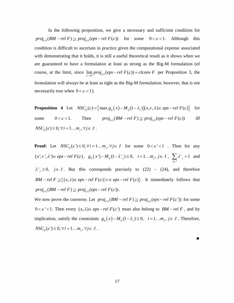
In the following proposition, we give a necessary and sufficient condition for

( ) ( )( ) ( ( ))x xproj BM rel F proj eps rel F for some 0 1 . Although this

condition is difficult to ascertain in practice given the computational expense associated

with demonstrating that it holds, it is still a useful theoretical result as it shows when we

are guaranteed to have a formulation at least as strong as the Big-M formulation (of

course, at the limit, since ( )

0lim ( ( ))xproj eps rel F clconv F

per Proposition 3, the

formulation will always be at least as tight as the Big-M formulation; however, that is not

necessarily true when 0 1 ).

Proposition 4 Let ( ) max (1 ) ( , , ) ( )ij ij ij jNSC g x M x eps rel F for

some 0 1 . Then ( ) ( )( ) ( ( ))x xproj BM rel F proj eps rel F iff

( ) 0, 1 ,ij jNSC i m j J .

Proof: Let ( ') 0, 1 ,ij jNSC i m j J for some 0 ' 1 . Then for any

( ', ', ') ( )x eps rel F , ' (1 ' ) 0, 1 ,ij ij j jg x M i m j J , ' 1j

j J

and

' 0,j j J . But this corresponds precisely to (22) – (24), and therefore

( , ) ( ) | ( )BM rel F x eps rel F eps rel F . It immediately follows that

( ) ( )( ) ( ( ))x xproj BM rel F proj eps rel F .

We now prove the converse. Let ( ) ( )( ) ( ( '))x xproj BM rel F proj eps rel F for some

0 ' 1 . Then every ( , ) ( ')x eps rel F must also belong to BM rel F , and by

implication, satisfy the constraints (1 ) 0, 1 ,ij ij j jg x M i m j J . Therefore,

( ') 0, 1 ,ij jNSC i m j J .

■

18

4. Illustrative Computational Results

In this section, we present illustrative computational results using our novel

formulation discussed in Section 3 to generate -approximate representations of the

convex hull of several classes of disjunctive convex sets within the context of

Generalized Disjunctive Programming (or equivalently, 0-1 indicator-induced MINLPs).

We focus on the so-called Synthesis, Retrofit-Synthesis and Constrained Layout

problems, although we note that this -approximate representation can be applied to

explicitly describe the convex hull of any nonlinear disjunctive convex set described by

(2), assuming the condition in (4) holds. For details about the general disjunctive

programming formulations of these problems, we refer the interested reader to the

Appendix, as well as to Sawaya’s thesis [44].

Our approach here consists of converting the disjunctive convex set F into the

-approximate set ( ) ( , , ) ( ) {0,1},jeps MIP F x eps rel F j J as

described in Section 3. We note that if the terms of the disjunctive set in GDP form do

not contain bounds, then we add those explicitly to ensure that the condition in (4) is met

(this is often the easiest way to ensure that (4) holds and is typically the approach used

within the GDP community). If the problem contains more than one disjunction k K ,

then every disjunctive set F is converted into its -approximate form and the resulting

algebraic sets are intersected to obtain, following Balas’ nomenclature in [3] for linear

disjunctive sets, the so-called “hull reformulation” ( ) ( )HR

k

k K

eps MIP eps MIP F

.

We conduct our computational experiments as a function of the parameter in order to

assess the sensitivity of the reformulation to this parameter. We also compare our

reformulation against the Big-M formulation, where every disjunctive convex set F is

converted into the set ( , ) {0,1},jBM MIP F x BM rel F j J to have a

point of reference when assessing the strength of our reformulation’s relaxation. We note

that the approach taken in these computational experiments is one of many approaches

that could have been taken using our reformulation. Alternatively, a hybrid approach of

converting only some disjunctive sets into their -approximate form while converting

19

others to their Big-M form could have been used; or intersecting certain disjunctive sets

first via basic steps (see [3] for details on basic steps) before converting them into their

-approximate forms (to strengthen the resulting relaxation) could have been performed;

or even using our new -approximate formulation within the context of a nonlinear cut-

generating program (whose cutting planes can be added to strengthen the big-M

formulation) could have been entertained (see [44, 47] for preliminary efforts in that

direction). As such, we emphasize that these computational experiments are merely

illustrative and are meant to show that this new reformulation “works” in practice. A

comprehensive computational study comparing the various approaches that could be used

with our reformulation against other approaches in the literature is out of scope for this

paper, but remains interesting future work.

The computations were performed using a nonlinear programming-based branch-

and-bound method (GAMS/SBB with CONOPT as the NLP solver) [10] with a 5 hour

time limit on a 2.4 GHz / 8GB RAM Linux PC. The computational time is reported in

seconds for 52 total instances, including 24 Synthesis, 22 Retrofit Synthesis and 6

Constrained Layout problems. In the computations, values for ε ranging from 10-10 to

0.99 are tested using the new ε-approximation formulation and compared with the classic

Big-M formulation (the values of the Big-M parameters were chosen for each nonlinear

inequality by solving for

maxjk

ijk ijkx C

M g x

for every , , i I j J k K ). We also note

that all instances solved in this section were submitted to MINLPLib [41] and are

available online.

Tables 2 through 4 show the number of instances from each class of problems that

were solvable, and Table 5 combines all of them into a single solution set. As can be

seen, using a value for ε of 10-10 results in an increased number of numerical failures in

the NLP sub-problems due to CONOPT not being able to converge to a feasible solution,

most likely due to the ill-conditioning of the Hessian of the approximation function as ε

tends to zero. On the other hand, using a value for ε above 0.1 tends to reach the time

limit for some of the Retrofit problems, most likely due to having weaker relaxations

(similarly for the Big-M formulations). This suggests that choosing a value of ε that is not

too small, to avoid potential numerical difficulties, nor too large, to avoid “loose”

relaxations that cause problems to “time-out”, is best. Indeed, by choosing a value of ε

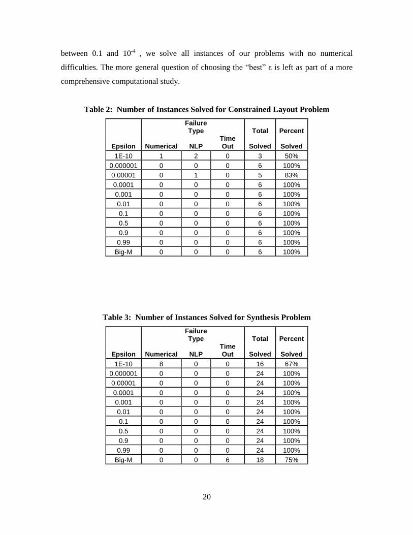
20

between 0.1 and 10-4 , we solve all instances of our problems with no numerical

difficulties. The more general question of choosing the “best” ε is left as part of a more

comprehensive computational study.

Table 2: Number of Instances Solved for Constrained Layout Problem

Failure Type Total Percent

Epsilon Numerical NLP Time Out Solved Solved

1E-10 1 2 0 3 50%

0.000001 0 0 0 6 100%

0.00001 0 1 0 5 83%

0.0001 0 0 0 6 100%

0.001 0 0 0 6 100%

0.01 0 0 0 6 100%

0.1 0 0 0 6 100%

0.5 0 0 0 6 100%

0.9 0 0 0 6 100%

0.99 0 0 0 6 100%

Big-M 0 0 0 6 100%

Table 3: Number of Instances Solved for Synthesis Problem

Failure Type Total Percent

Epsilon Numerical NLP Time Out Solved Solved

1E-10 8 0 0 16 67%

0.000001 0 0 0 24 100%

0.00001 0 0 0 24 100%

0.0001 0 0 0 24 100%

0.001 0 0 0 24 100%

0.01 0 0 0 24 100%

0.1 0 0 0 24 100%

0.5 0 0 0 24 100%

0.9 0 0 0 24 100%

0.99 0 0 0 24 100%

Big-M 0 0 6 18 75%

21

Table 4: Number of Instances Solved for Retrofit-Synthesis Problem

Failure Type Total Percent

Epsilon Numerical NLP Time Out Solved Solved

1E-10 18 0 0 4 18%

0.000001 1 0 0 21 95%

0.00001 0 0 0 22 100%

0.0001 0 0 0 22 100%

0.001 0 0 0 22 100%

0.01 0 0 0 22 100%

0.1 0 0 0 22 100%

0.5 0 0 3 19 86%

0.9 0 0 3 19 86%

0.99 0 0 2 20 91%

Big-M 0 0 18 4 18%

Table 5: Number of Instances Solved for All Problem Classes

Failure Type Total Percent

Epsilon Numerical NLP Time Out Solved Solved

1E-10 27 2 0 23 44%

0.000001 1 0 0 51 98%

0.00001 0 1 0 51 98%

0.0001 0 0 0 52 100%

0.001 0 0 0 52 100%

0.01 0 0 0 52 100%

0.1 0 0 0 52 100%

0.5 0 0 3 49 94%

0.9 0 0 3 49 94%

0.99 0 0 2 50 96%

Big-M 0 0 24 28 54%

Table 6 presents the results of solving the root relaxation of all instances

( )HReps MIP for various values of (i.e. we are solving the NLP

( ) ( )HR

k

k K

eps rel eps rel F

). The CONOPT solver was used to solve this

resulting NLP, and the relaxation gap, which is defined as

22

( ) ( )( )

( )

HR HR

HR

Optimal Value eps MIP Optimal Value eps relGAP

Optimal Value eps MIP

, is reported.

The GAP is a useful indicator of the strength of the formulation, as a smaller GAP

typically leads to shorter solution times. As expected, the use of the ε-approximation

formulation leads to a relaxation at least as strong as the Big-M formulation for all

instances, and one that is significantly stronger for instances of the Synthesis and Retrofit

problems. However, we note that for ε values of 10-10, 12 of 22 retrofit instances

experienced numerical errors in solving the root relaxation. Furthermore, a clear increase

in GAP is evident as ε increases for the synthesis and retrofit instances. Finally,

Constrained Layout instances show no difference in relaxation strength between ε and

Big-M reformulations.

Table 6: Solution of the Root Relaxation

Constrained

Layout Synthesis Retrofit-

Synthesis

Epsilon Avg Gap Low Gap

High Gap

Avg Gap Low Gap

High Gap

Avg Gap Low Gap

High Gap

1E-10 100% 100% 100% 2% 0% 17% 6% 1% 10%

0.000001 100% 100% 100% 2% 0% 17% 4% 0% 10%

0.00001 100% 100% 100% 2% 0% 17% 4% 0% 10%

0.0001 100% 100% 100% 2% 0% 17% 4% 0% 10%

0.001 100% 100% 100% 2% 0% 17% 4% 0% 10%

0.01 100% 100% 100% 2% 0% 17% 4% 1% 10%

0.1 100% 100% 100% 2% 0% 21% 5% 2% 10%

0.5 100% 100% 100% 5% 0% 44% 12% 2% 25%

0.9 100% 100% 100% 7% 0% 66% 17% 3% 38%

0.99 100% 100% 100% 8% 0% 72% 19% 3% 40%

Big-M 100% 100% 100% 435% 19% 2608% 320% 57% 876%

Table 7 compares cumulative results for the subset of instances in which the Big-

M formulation and the ( )HReps MIP formulation for all ε values were solvable within

the time limit; these instances are referred to as “shared” instances in the table, for which

we report the cumulative number of branch-and-bound nodes and the cumulative run

time. For Synthesis and Retrofit instances, the Big-M formulations require substantially

longer run-times than those with the ε-approximation formulation due to much weaker

relaxations. Furthermore, values of ε in the range of 0.1 to 0.001 appear to have the best

23

range of performance. However, for the Constrained Layout instances, the Big-M

formulations outperform the ε-approximation formulations given the fact that we are

solving a smaller problem whose relaxation is no worse than the ε-approximation

formulations.

Table 7: Cumulative Results for Instances Solvable by all Approaches

Constrained Layout

Synthesis

Retrofit-Synthesis

Epsilon Shared Nodes Time (sec) Nodes/sec Shared Nodes Time (sec) Nodes/sec Shared Nodes Time (sec) Nodes/sec

1E-10 3 3882750 3797 1023 16 108 8 13 4 1328 16 81

0.000001 3 4767347 5491 868 16 113 6 18 4 1265 11 117

0.00001 3 3018376 2760 1094 16 143 6 23 4 1362 10 135

0.0001 3 1797986 1467 1226 16 188 8 25 4 1252 9 143

0.001 3 2204085 1861 1184 16 190 7 27 4 1267 7 183

0.01 3 2204085 1859 1185 16 190 7 27 4 1330 7 186

0.1 3 2497305 1642 1521 16 192 7 27 4 1442 7 193

0.5 3 1424466 727 1960 16 250 8 30 4 3263 19 174

0.9 3 1799602 947 1900 16 408 11 37 4 5594 36 157

0.99 3 1579994 834 1895 16 522 14 38 4 6105 43 143

Big-M 3 382858 43 9006 16 1682571 17801 95 4 990966 1566 633

5 Conclusion

In this paper, we have developed an explicit algebraic representation for general

disjunctive convex sets using the perspective function that yields tight relaxations, while

avoiding the computational challenges resulting from the functional form of the

perspective function. We have shown that this new algebraic representation can be used

to generate Mixed-Integer Programming reformulations that are exactly equivalent to the

original disjunctive convex set. Furthermore, we have shown that this algebraic

representation is equivalent to the closure of the convex hull of the disjunctive convex set

at its limit. Finally, and importantly, this representation facilitates implementation in

general purpose algebraic modeling languages and uses general purpose solvers. We also

note that this representation can be used in the generation of cutting planes for problems

that contain disjunctive convex sets as part of their formulation or from disjunctions that

are generated from an MINLP formulation, although the details of these approaches are

24

not covered in this paper. A logical next step is to compare the use of our reformulation

within the context of different algorithmic approaches (e.g. its performance as an explicit

algebraic representation of the disjunctive convex set versus its use in a nonlinear cut-

generating program) against the various other approaches in the literature previously

discussed in order to assess which methods work best on which classes of problems.

Appendix. Description of nonlinear GDP problem classes

Synthesis of Process Networks

These problems consist in determining those process units kY to be included in

the design of a process network such that the structure and operating conditions of this

network will meet certain design specifications, while minimizing the sum of fixed costs

kc and variable costs Ta x of the overall network (the variable x represents material

flow). The following example represents a GDP model of a 5-process network, and can

be found in Sawaya’s thesis [44]. This example is a slightly modified version of the

original form proposed by Duran and Grossmann [13] (MINLP form), Turkay and

Grossmann [48] and Lee and Grossmann [37] (GDP forms).

25

5

1

1 2 3

6 4 5

min

. .

0 (25)

0

T

k

k

Z c a x

s t

x x x

x x x

6 7 8 11

(26)

0 x x x x

8 9 10 11

1

4 2

1

(27)

0 (28)

exp( ) 1 0

5

x x x x

Y

x x

c

1

4 2

1

2 2

5 3 3 5

2 2

0 (29)

0

exp( /1.2) 1 0 0

8 0

Y

x x

c

Y Y

x x x x

c c

3 3

13 9 9 13

3 3

(30)

0.75 0 0

6 0

Y Y

x x x x

c c

(31)

4 4

14 10 10 14

4 4

5

5

15 11

11 12

15 12

5

exp( /1.5) 1 0 0 (32)

10 0

0

0.5 0

6

Y Y

x x x x

c c

YY

x xx x

x x

c

15

5

1 12

0 (33)

0

10, 7

x

c

x x

1 2

(34)

Y Y (35)

[0,0,0,0,0,0,5,0,0,0,0, 2,200,250,300]

, 0, { , } for =1,2,...5 ; =1,2,...15

T

j k k

a

x c Y True False k j

Equations (25)-(28) represent linear mass balances around nodes N1-N4.

Disjunctions (29)-(33) embody the discrete dichotomy of process selection, where a unit,

along with its in-and-out flows (connected to one another via an exponential relationship)

and fixed cost, is selected for inclusion in the final network only if its corresponding

Boolean variable kY True ; otherwise, the unit is not selected, and its flows and fixed

cost are set to 0. Equation (34) represents upper bounds on certain flows, and finally,

26

logic equation (35) imposes the condition that either process 1 or 2 must be selected (but

not both).

Retrofit-Synthesis of Process Networks

These problems consist in simultaneously redesigning part of an existing plant

and synthesizing (from scratch) part of a new one. Specifically, one is interested in

determining whether certain units should be included in the design of the new plant, and

whether certain modifications such as improvements in yield, capacity and energy

reduction should be performed on the existing plant. In addition it is required that

economic potential be maximized given a certain time horizon and limited capital

investments. The nonlinearities in this set of problems stem from the synthesis portion of

the model, and correspond to logarithmic functions. Below, we only show the retrofit

portion of the model (since the Synthesis portion was presented above), which is a

modification of work by Jackson and Grossmann [33] and which appeared in [44]:

27

(36)

. .

prod raw

t t t t t t

s s s s

t T s S t T s S t T t T

t t

p

t T p P t T

t t

s s s

Min PR mf PR mf PRSTqst PRWTqwt

fc ec

s t mf f MW

, (37)

, (38) t t

s s prod

t

s

s S t T

mf DEM s S t T

mf SU

, (39)

,

n nin out

t

s raw

t t

s s

s S s S

P s S t T

mf mf n N t T

(40)

, (41)

( )

p pin out

pm

lmt

lmt

t t t

s s p

s S s S

t

tt t s

s p

m M p

mf mf unrct p P t T

Y

GMAf f

GMA

, , (42)

,

out

p in

pm

t

pm p

t t

s pm

s S

t

t tm M p pm

ETA s S p P t T

mf CAP

Wp P t T

fc FC

(43)

( ) , , (44)

( )

out ink k

in outk k

t t t t

sk s s s s cold

t t t t

sk s s s s

q mf CP T T s S k K t T

q mf CP T T

2

1 1

, , (45)

k k

hot cold

cold

hot

hot

t

t t t t t t t

k k sk sk

s S s St t

sk

k K s S

t t

sk

k K s S

s S k K t T

X

X r r qst qwt q q

qst q

qwt q

, (46)k

k

t t

k K

t t t

K

k K

k K t Tqst qst

qwt r qwt

28

1 2

1 2

(47)

raw

t t

t t t t

t t t t t t t

p s s

p P s S

V Vt T

ec EFC ec EFC

fc ec PR mf PRSTqst PRWTqwt INV

1

1

(48)

, , \ (49)

pm pm

pm p

t

t

t t

t

t T

Y Y p P t T m M m

W W

1 1

1 , , \ (50)

, (51)

p p

pm pm pm

t t

t t

t

p P t T m M m

Y W p P t T

Y Y W

1

1

, , \ (52)

, \ j j

t

t

p P t T m M m

X X t T j J j

1

1 1

1

(53)

, \ (54)

j

t t

t

t t

V V t T j J j

X V

1

1

(55)

, \ (56)

,

j j j

t t

t

t t

s s

t T

X X V t T j J j

mf f

1

,

,

, , , t t t

lmt p p p

s S t T

f unrct fc p P t T

1

1

, ,

, ,

t

sk

t t t

q s S k K t T

qst qwt ec

1

, , ,

, ,

k k

pm pm

t t t

k

t t

t T

qst qwt r k K t T

Y W True F

, ,

, , , j j

t t

alse p P t T m M

X V True False j J t T

The objective function (36) includes revenues from sales, costs of raw material,

utility costs, as well as capital costs t

pfc and energy costs tec over time periods t T .

Equation (37) represents an equivalence relation between mass and molar flow rates,

equations (38) and (39) ensure that mass flow rates for products and raw materials are

respectively bounded by demand and supply parameters, and equations (40) and (41)

serve as mass balances around nodes n N and processes p P , respectively. The first

set of disjunctions (42) selects one of the operating modes for the retrofit project m M ,

for every process p P , in every time period t T , where projects m include modifying

either nothing at all ( 1m M ), process conversion ( 2m M ), capacity ( 3m M ) or both

( 4m M ). The second set of disjunctions (43) enforces the cost of the aforementioned

29

modifications, where capital costs are set to zero ( t

pfc = 0) if nothing is modified.

Equations (44) and (45) serve as equivalence relations between energy and mass flow

rate variables, while disjunction(s) (46) select the appropriate operating mode j

tX

j J so that 1

tX corresponds to no energy integration and 2

tX enforces the

transshipment equations. Through Boolean variables j

tV , the set of disjunctions (47)

enforce the cost associated with energy reduction, where these costs are set to zero ( tec =

0) if nothing is modified ( 1

tV = True). Equation (48) limits the expenses for the retrofit

project. Equations (51) and (52), (55) and (56) are logical conditions that connect,

respectively, disjunctions (42) to (43) and disjunctions (44) to (45) with each other, and

equations (49) and (50), (53) and (54) impose logical conditions between disjuncts in

every set of corresponding disjunctions. Essentially, these logical equations constrain the

problem such that costs associated with conversion and/or capacity are enforced exactly

once for every process p P in every time period t T , and such that costs associated

with energy reduction are enforced exactly once per time period t T .

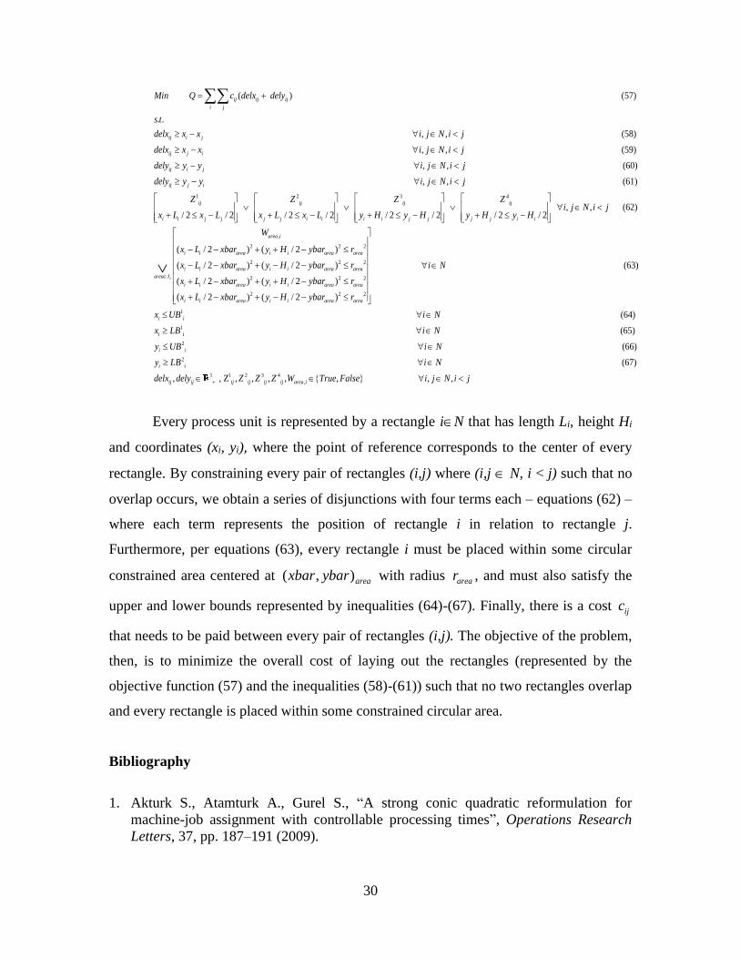
Constrained Layout

In these problems, which first appeared in [45] (see also [44]), non-overlapping

process units represented by rectangles must be placed within the confines of certain

designated areas formulated as circular nonlinear constraints, such that the cost of

connecting these units is minimized. The nonlinearities in this set of problems are all

quadratic and correspond to Euclidean-distance constraints, and the integrality gap for all

instances presented is equal to 100%. Note that these problem are intentionally poorly

modeled in order to have a large integrality gap and no feasible solution near the optimal

solution of the continuous relaxation.

30

( ) (57)

. .

ij ij ij

i j

Min Q c delx dely

s t

, , (58) ij i j

ij

delx x x i j N i j

delx

, , (59)

j i

ij i j

x x i j N i j

dely y y

, , (60)

ij j i

i j N i j

dely y y

1 2

, , (61)

/ 2 / 2

ij ij

i i j j j j

i j N i j

Z Z

x L x L x L

3 4

,

2 2 2

2

, , (62) / 2 / 2 / 2 / 2 / 2 / 2

( / 2 ) ( / 2 )

( / 2 ) ( / 2

i

ij ij

i i i i j j j j i i

area i

i i area i i area area

i i area i i are

area J

Z Zi j N i j

x L y H y H y H y H

W

x L xbar y H ybar r

x L xbar y H ybar

2 2

2 2 2

2 2 2

)

( / 2 ) ( / 2 )

( / 2 ) ( / 2 )

a area

i i area i i area area

i i area i i area area

r i N

x L xbar y H ybar r

x L xbar y H ybar r

1

(63)

i ix UB i N

1

(64)

i ix LB i N

2

(65)

i iy UB i N

2

(66)

i iy LB i N

1 1 2 3 4

,

(67)

, , Z , , , , , , , ij ij ij ij ij ij area idelx dely Z Z Z W True False i j N i j

Every process unit is represented by a rectangle iN that has length Li, height Hi

and coordinates (xi, yi), where the point of reference corresponds to the center of every

rectangle. By constraining every pair of rectangles (i,j) where (i,j N, i < j) such that no

overlap occurs, we obtain a series of disjunctions with four terms each – equations (62) –

where each term represents the position of rectangle i in relation to rectangle j.

Furthermore, per equations (63), every rectangle i must be placed within some circular

constrained area centered at ( , )areaxbar ybar with radius arear , and must also satisfy the

upper and lower bounds represented by inequalities (64)-(67). Finally, there is a cost ijc

that needs to be paid between every pair of rectangles (i,j). The objective of the problem,

then, is to minimize the overall cost of laying out the rectangles (represented by the

objective function (57) and the inequalities (58)-(61)) such that no two rectangles overlap

and every rectangle is placed within some constrained circular area.

Bibliography

1. Akturk S., Atamturk A., Gurel S., “A strong conic quadratic reformulation for

machine-job assignment with controllable processing times”, Operations Research

Letters, 37, pp. 187–191 (2009).

31

2. Balas E., “Disjunctive Programming”, Annals of Discrete Mathematics, 5, 3-51,

(1979).

3. Balas E., “Disjunctive Programming and a Hierarchy of Relaxations for Discrete

Continuous Optimization Problems”, SIAM J. Alg. Disc. Meth., Vol. 6, No. 3 (1985).

4. Balas E., “Disjunctive Programming: Properties of the Convex Hull of Feasible

Points”, Invited paper, with a foreword by G. Cornuejols and W. Pulleybank, Discrete

Applied Mathematics, 89, 3-44, (1998). (Originally MSRR #348, Carnegie Mellon

University, July 1974).

5. Bertsekas D., Gallager R., “Data Networks”, Prentice-Hall, Englewood Cliffs, NJ,

(1987).

6. Bonami P., “Lift-and-Project Cuts for Mixed Integer Convex Programs”, IPCO 2011,

Lecture Notes in Computer Science 6655, pp. 52-64 (2011)

7. Bonami P., Lodi A., Tramontani A., Wiese S., "On mathematical programming with

indicator constraints." Mathematical Programming 151.1 pp. 191-223 (2015)

8. Bonami P., Tramontani A., “Advances in CPLEX for Mixed Integer Nonlinear

Optimization”, Presentation at ISMP Pittsburgh (2015)

9. Boorstyn R., Frank H., “Large-scale network topological optimization”, IEEE

Transactions on Communications, 25 pp. 29–47 (1977).

10. Brooke A., Kendrick D., Meeraus A., Raman R., “GAMS language guide”, Version

98, GAMS Development Corporation, Washington D.C.

SBB: https://www.gams.com/latest/docs/S_SBB.html

CONOPT: https://www.gams.com/latest/docs/S_CONOPT.html

11. Castro P.M., Grossmann I.E., “Generalized Disjunctive Programming as a Systematic

Modeling Framework to Derive Scheduling Formulations,” Ind. Eng. Chem. Res 51,

5781−5792 (2012).

12. Ceria S., Soares J., “Convex programming for disjunctive optimization”,

Mathematical Programming, 86 (3), 595-614 (1999).

13. Duran M.A., Grossmann I.E., "An Outer Approximation Algorithm for a Class of

Mixed Integer Nonlinear Programs," Mathematical Programming 36, 307-339,

(1986)

14. Elhedhli S., “Service system design with immobile servers, stochastic demand, and

congestion”, Manufacturing and Service Operations Management, 8 pp. 92–97

(2006).

32

15. Ferris M.C., Dirkse S.P., Jagla J.H. and Meeraus A., "An Extended Mathematical

Programming Framework", Computers and Chemical Engineering. Vol. 33 pp. 1973-

1982 (2009); see also https://www.gams.com/latest/docs/UG_EMP.html

16. Frangioni A., Gentile C., “Perspective cuts for a class of convex 0-1 mixed integer

programs”, Mathematical Programming 106, 225–236, (2006)

17. Frangioni A., Gentile C., “SDP diagonalizations and perspective cuts for a class of

nonseparable MIQP”, Operations Research Letters 35(2), 181–185 (2007)

18. Frangioni A., Gentile C., “A computational comparison of reformulations of the

perspective relaxation: SOCP vs. cutting planes”, Operations Research Letters 37(3),

206–210 (2009)

19. Frangioni A., Gentile C., Grande E., Pacifici A., “Projected Perspective

Reformulations with Applications in Design Problems” Operations Research 59:5,

1225-1232 (2011)

20. Furman K.C., “Private Communication to Sawaya” (2005)

21. Furman K.C., Sawaya N.W., Grossmann I.E., “An exact MINLP formulation for

nonlinear disjunctive programs based on the convex hull”, Presentation at 20th

International Symposium on Mathematical Programming (2009)

22. Furman K.C., Sawaya N.W., Grossmann I.E., “A useful algebraic representation of

convex sets using the perspective function”, Presentation at MINLP Pittsburgh (2014)

23. Grossmann I.E., Westerberg A.W., Biegler L.T., "Retrofit Design of Chemical

Processes," Proceedings of Foundations of Computer Aided Process Operations (Eds.

G.V. Reklaitis and H.D. Spriggs, Elsevier), 403 (1987).

24. Grossmann I.E., Caballero J.A, Yeomans H., "Mathematical Programming

Approaches for the Synthesis of Chemical Process Systems," Korean J. Chem.Eng.,

16, 407-426 (1999).

25. Grossmann I.E., Lee S., "Generalized Disjunctive Programming: Nonlinear Convex

Hull Relaxation and Algorithms", Computational Optimization and Applications, 26,

83-100, (2003).

26. Gunluk O., Lee J., Weismantel R., “MINLP strengthening for separable convex

quadratic transportation-cost UFL”, Tech. Rep. RC24213 (W0703-042), IBM

Research Division, (March 2007).

27. Gunluk O., Linderoth J., “Perspective relaxation of mixed integer nonlinear programs

with indicator variables”, in: A. Lodi, A. Panconesi, G. Rinaldi (eds.) Integer

33

Programming and Combinatorial Optimization, Lecture Notes in Computer Science,

vol. 5035, pp. 1–16. Springer Berlin / Heidelberg (2008)

28. Gunluk O., Linderoth J., “Perspective reformulations of mixed integer nonlinear

programs with indicator variables”, Mathematical Programming 124, 183–205 (2010)

29. Gunluk, O., Linderoth J., “Perspective reformulation and Applications”, Mixed

Integer Nonlinear Programming, The IMA Volumes in Mathematics and its

Applications Volume 154, pp 61-89, (2012)

30. Hart W.E., Laird C.D., Watson J.P., Woodruff D.L., Hackebeil G.A., Nicholson B.L.,

Siirola J.D. “Generalized Disjunctive Programming. In: Pyomo — Optimization

Modeling in Python”, Springer Optimization and Its Applications, vol 67, Springer

(2017)

31. Hijazi H., Bonami P., Cornujols G., Ouorou A.: “Mixed Integer Non Linear Programs

featuring “On/Off” constraints: convex analysis and applications” Electronic Notes in

Discrete Mathematics 36, 1153–1160 (2010). ISCO 2010 - International Symposium

on Combinatorial Optimization

32. Hiriart-Urruty J., Lemaréchal C., “Fundamentals of Convex Analysis”, 2nd edition,

Springer-Verlag, (2004).

33. Jackson J., Grossmann I.E., “High-Level optimization model for the retrofit planning

of process networks”, Ind. Eng. Chem. Res., 41, 3762-3770, (2002).

34. Jackson J., Grossmann I.E., “A Disjunctive Programming Approach for the Optimal

Design of Reactive Distillation Columns”, Computers and Chemical Engineering, 25,

1661-1673, (2001).

35. Jeroslow R.G., “Representability in Mixed Integer Programming, I: Characterization

Results”, Discrete Applied Mathematics, 17, 223-243, (1987).

36. Kilinc M., Linderoth J., Luedtke J., “Lift-and-Project Cuts for Convex Mixed Integer

Nonlinear Programs”, Mathematical Programming Computation, 9, 499-526 (2017)

37. Lee S., Grossmann I.E., “New Algorithms for Nonlinear Generalized Disjunctive

Programming”, Computers and Chemical Engineering, 24, 2125-2141, (2000).

38. Lee S., Grossmann I.E.: “Erratum to ”New Algorithms for Nonlinear Generalized

Disjunctive Programming”, Comp. and Chem. Eng. 24, 1153 (2001)

39. Lee S., Grossmann I.E.: “Logic-Based Modeling and Solution of Nonlinear

Discrete/Continuous Optimization Problems” Annals of Op. Res. 139, 267–288

(2005)

34

40. Mendez C.A., Cerdá J., Grossmann I.E., Harjunkoski I., Fahl M., “State-Of-The-Art

Review of Optimization Methods for Short-Term Scheduling of Batch Processes,”

Computers and Chemical Engineering 30, 913-946 (2006).

41. MINLPLib, A Library of Mixed-Integer and Continuous Nonlinear Programming

Instances, available at http://www.minlplib.org/index.html

42. Raman R., Grossmann I.E., “Modeling and Computational Techniques for Logic

Based Integer Programming”, Computers and Chemical Engineering, 18 (7), 563-

578, (1994).

43. Ravemark E. “Optimization models for design and operation of chemical batch

processes”, Ph.D. Thesis, ETH Zurich, (1995)

44. Sawaya N.W. “Reformulations, Relaxations and Cutting Planes for Generalized

Disjunctive Programming”, Ph.D. Thesis, Carnegie Mellon University (2006)

45. Sawaya N.W., Grossmann I.E., “Computational Implementation of Non-linear

Convex Hull Reformulation”, Computers and Chemical Engineering, 31, 856-866,

(2007).

46. Stubbs R., Mehrotra S., “A Branch-and-Cut Method for 0-1 Mixed Convex

Programming”, Mathematical Programming 86, 515-532, (1999)

47. Trespalacios F., Grossmann I.E., “Cutting Plane Algorithm for Convex Generalized

Disjunctive Programs”, INFORMS Journal on Computing, 28, 209-222 (2016)

48. Turkay M., Grossmann I.E., “Logic-Based MINLP Algorithms for the Optimal

Synthesis of Process Networks”, Computers and Chemical Engineering, 20 (8), 959-

978, (1996).

49. Vecchietti A., “LOGMIP 2.0 User Manual” (2011)

http://www.logmip.ceride.gov.ar/files/pdfs/newUserManual.pdf

50. Vecchietti A., Lee S., Grossmann I.E., “Modeling of Discrete/Continuous

Optimization Problems: Characterization and Formulation of Disjunctions and Their

Relaxations”, Comp. and Chem. Eng. 27, 433–448 (2003)

51. Wood A., Wollemberg B., “Power Generation Operation and Control”, John Wiley

and Sons, (1996).

52. Wu H., Wen H., Zhu Y., “Branch-and-Cut Algorithmic Framework for 0-1 Mixed-

Integer Convex Nonlinear Programs”, Ind. and Eng. Chem. Res. 48, 9119–9127

(2009)

35

53. Zhu Y., Kuno T., “A Disjunctive Cutting-Plane Based Branch-and-Cut Algorithm for

0-1 Mixed-Integer Convex Nonlinear Programs”, Ind. and Eng. Chem. Res. 45(1),

187–196 (2006)