abaqus release notes - mathematics · pdf fileabaqus 6.11 release. ... cfd simulation...
TRANSCRIPT

Abaqus Release Notes
Abaqus ID:
Printed on:
Abaqus 6.12Release Notes


Abaqus
Release Notes
Abaqus ID:
Printed on:

Legal NoticesCAUTION: This documentation is intended for qualified users who will exercise sound engineering judgment and expertise in the use of the Abaqus
Software. The Abaqus Software is inherently complex, and the examples and procedures in this documentation are not intended to be exhaustive or to apply
to any particular situation. Users are cautioned to satisfy themselves as to the accuracy and results of their analyses.
Dassault Systèmes and its subsidiaries, including Dassault Systèmes Simulia Corp., shall not be responsible for the accuracy or usefulness of any analysis
performed using the Abaqus Software or the procedures, examples, or explanations in this documentation. Dassault Systèmes and its subsidiaries shall not
be responsible for the consequences of any errors or omissions that may appear in this documentation.
The Abaqus Software is available only under license from Dassault Systèmes or its subsidiary and may be used or reproduced only in accordance with the
terms of such license. This documentation is subject to the terms and conditions of either the software license agreement signed by the parties, or, absent
such an agreement, the then current software license agreement to which the documentation relates.
This documentation and the software described in this documentation are subject to change without prior notice.
No part of this documentation may be reproduced or distributed in any form without prior written permission of Dassault Systèmes or its subsidiary.
The Abaqus Software is a product of Dassault Systèmes Simulia Corp., Providence, RI, USA.
© Dassault Systèmes, 2012
Abaqus, the 3DS logo, SIMULIA, CATIA, and Unified FEA are trademarks or registered trademarks of Dassault Systèmes or its subsidiaries in the United
States and/or other countries.
Other company, product, and service names may be trademarks or service marks of their respective owners. For additional information concerning
trademarks, copyrights, and licenses, see the Legal Notices in the Abaqus 6.12 Installation and Licensing Guide.
Abaqus ID:
Printed on:
Locations
SIMULIA Worldwide Headquarters Rising Sun Mills, 166 Valley Street, Providence, RI 02909–2499, Tel: +1 401 276 4400,
Fax: +1 401 276 4408, [email protected], http://www.simulia.com
SIMULIA European Headquarters Stationsplein 8-K, 6221 BT Maastricht, The Netherlands, Tel: +31 43 7999 084,
Fax: +31 43 7999 306, [email protected]
Dassault Systèmes’ Centers of Simulation Excellence
United States Fremont, CA, Tel: +1 510 794 5891, [email protected]
West Lafayette, IN, Tel: +1 765 497 1373, [email protected]
Northville, MI, Tel: +1 248 349 4669, [email protected]
Woodbury, MN, Tel: +1 612 424 9044, [email protected]
Mayfield Heights, OH, Tel: +1 216 378 1070, [email protected]
Mason, OH, Tel: +1 513 275 1430, [email protected]
Warwick, RI, Tel: +1 401 739 3637, [email protected]
Lewisville, TX, Tel: +1 972 221 6500, [email protected]
Australia Richmond VIC, Tel: +61 3 9421 2900, [email protected]
Austria Vienna, Tel: +43 1 22 707 200, [email protected]
Benelux Maarssen, The Netherlands, Tel: +31 346 585 710, [email protected]
Canada Toronto, ON, Tel: +1 416 402 2219, [email protected]
China Beijing, P. R. China, Tel: +8610 6536 2288, [email protected]
Shanghai, P. R. China, Tel: +8621 3856 8000, [email protected]
Finland Espoo, Tel: +358 40 902 2973, [email protected]
France Velizy Villacoublay Cedex, Tel: +33 1 61 62 72 72, [email protected]
Germany Aachen, Tel: +49 241 474 01 0, [email protected]
Munich, Tel: +49 89 543 48 77 0, [email protected]
India Chennai, Tamil Nadu, Tel: +91 44 43443000, [email protected]
Italy Lainate MI, Tel: +39 02 3343061, [email protected]
Japan Tokyo, Tel: +81 3 5442 6302, [email protected]
Osaka, Tel: +81 6 7730 2703, [email protected]
Korea Mapo-Gu, Seoul, Tel: +82 2 785 6707/8, [email protected]
Latin America Puerto Madero, Buenos Aires, Tel: +54 11 4312 8700, [email protected]
Scandinavia Stockholm, Sweden, Tel: +46 8 68430450, [email protected]
United Kingdom Warrington, Tel: +44 1925 830900, [email protected]
Authorized Support Centers
Argentina SMARTtech Sudamerica SRL, Buenos Aires, Tel: +54 11 4717 2717
KB Engineering, Buenos Aires, Tel: +54 11 4326 7542
Solaer Ingeniería, Buenos Aires, Tel: +54 221 489 1738
Brazil SMARTtech Mecânica, Sao Paulo-SP, Tel: +55 11 3168 3388
Czech & Slovak Republics Synerma s. r. o., Psáry, Prague-West, Tel: +420 603 145 769, [email protected]
Greece 3 Dimensional Data Systems, Crete, Tel: +30 2821040012, [email protected]
Israel ADCOM, Givataim, Tel: +972 3 7325311, [email protected]
Malaysia WorleyParsons Services Sdn. Bhd., Kuala Lumpur, Tel: +603 2039 9000, [email protected]
Mexico Kimeca.NET SA de CV, Mexico, Tel: +52 55 2459 2635
New Zealand Matrix Applied Computing Ltd., Auckland, Tel: +64 9 623 1223, [email protected]
Poland BudSoft Sp. z o.o., Poznań, Tel: +48 61 8508 466, [email protected]
Russia, Belarus & Ukraine TESIS Ltd., Moscow, Tel: +7 495 612 44 22, [email protected]
Singapore WorleyParsons Pte Ltd., Singapore, Tel: +65 6735 8444, [email protected]
South Africa Finite Element Analysis Services (Pty) Ltd., Parklands, Tel: +27 21 556 6462, [email protected]
Spain & Portugal Principia Ingenieros Consultores, S.A., Madrid, Tel: +34 91 209 1482, [email protected]
Abaqus ID:
Printed on:

Taiwan Simutech Solution Corporation, Taipei, R.O.C., Tel: +886 2 2507 9550, [email protected]
Thailand WorleyParsons Pte Ltd., Singapore, Tel: +65 6735 8444, [email protected]
Turkey A-Ztech Ltd., Istanbul, Tel: +90 216 361 8850, [email protected]
Complete contact information is available at http://www.simulia.com/locations/locations.html.
Abaqus ID:
Printed on:
INTRODUCTION TO Abaqus 6.12
1. Introduction to Abaqus 6.12
This document introduces features in Abaqus that have been added, enhanced, or updated since the
Abaqus 6.11 release.
Chapter 1 provides a brief overview of the Abaqus products included in this release. Chapters 2–16
provide short descriptions of new Abaqus 6.12 features in Abaqus/Standard, Abaqus/Explicit, Abaqus/CFD,
and Abaqus/CAE, categorized by subject:
• Chapter 2, “General enhancements”: general changes to the Abaqus interface.
• Chapter 3, “Modeling”: features related to creating your model.
• Chapter 4, “Analysis procedures”: features related to defining an analysis.
• Chapter 5, “Analysis techniques”: features related to analysis techniques in Abaqus.
• Chapter 6, “Materials”: new material models or changes to existing material models.
• Chapter 7, “Elements”: new elements or changes to existing elements.
• Chapter 8, “Prescribed conditions”: loads, boundary conditions, and predefined fields.
• Chapter 9, “Constraints”: kinematic constraints.
• Chapter 10, “Interactions”: features related to contact and interaction modeling.
• Chapter 11, “Engineering features”: engineering features related to part and assembly modeling.
• Chapter 12, “Meshing”: features related to meshing your model.
• Chapter 13, “Execution”: commands and utilities for running any of the Abaqus products.
• Chapter 14, “Output and visualization”: obtaining, postprocessing, and visualizing results from Abaqus
analyses.
• Chapter 15, “User subroutines, utilities, and plug-ins”: additional user programs that can be run with
Abaqus.
• Chapter 16, “Abaqus Scripting Interface”: using the Abaqus Scripting Interface to write user scripts.
Each entry in these chapters clearly indicates the Abaqus product or products to which the feature applies and
includes cross-references to more detailed information. Chapter 17, “Summary of changes,” summarizes in
tabular format the changes to Abaqus keyword options, user subroutines, and output variable identifiers.
1.1 Key features of Abaqus 6.12
This section provides a list of themost significant new capabilities and enhancements available inAbaqus 6.12;
refer to the table of contents for a complete list of new features.
• Performance improvements:
– Batch preprocessing and initialization
– Substructure generation using AMS
– Multiple GPGPU cards
1–1
Abaqus ID:
Printed on:
INTRODUCTION TO Abaqus 6.12
• Associative import:
– Transfer an assembly from CATIA V6 to Abaqus/CAE
• Feature support in Abaqus/CAE:
– Time harmonic electromagnetic analysis
– Coupled thermal-electrical-structural analysis
– Surface fluid cavities and fluid exchanges
– Base motion boundary conditions and PSD amplitudes
– Contact stabilization, feature edges, and contact initialization
• New modeling options:
– Parallel network viscoelastic material model
– Thick-walled pipe elements
– Rotordynamic load
• Contact enhancements:
– Feature edge contact in Abaqus/Standard
– Eulerian-Lagrangian thermal contact
• Fluid analysis:
– Implicit advection
– Non-Newtonian viscosity
• Electromagnetic analysis:
– Magnetostatic analysis
– Transient eddy current analysis
– Nonlinear magnetic behavior
• Eulerian analysis:
– Adaptive mesh refinement
• General usability:
– Maximum damage initiation output in shells
– Tie constraint deletion with element erosion
• Abaqus/CAE usability:
– Plot and probe selected model data in the Visualization module
– Session object persistence
– Create geometry from orphan elements
– Boundary layer meshing
– Combine orphan and native mesh features in a part
1–2
Abaqus ID:
Printed on:
INTRODUCTION TO Abaqus 6.12
– Modify a mesh by dragging nodes
– View cut display
The remaining chapters in this book provide details on these and other new features of Abaqus 6.12. In
addition to the enhancements listed here, most of the known bugs in Abaqus 6.11 are corrected.
1.2 Abaqus products
Individual components of the Abaqus suite are described in this section.
Analysis• Abaqus/Standard: This general-purpose finite element analysis program includes all analysis
capabilities except nonlinear dynamic analysis using explicit time integration—provided in the
Abaqus/Explicit program—and the add-on analysis functionality described below.
• Abaqus/Explicit: This product provides nonlinear, transient, dynamic analysis of solids and structures
using explicit time integration. Its powerful contact capabilities, reliability, and computational efficiency
on large models also make it highly effective for quasi-static applications involving discontinuous
nonlinear behavior.
• Abaqus/CFD: This product is a computational fluid dynamics program with extensive support for
preprocessing, simulation, and postprocessing in Abaqus/CAE. Abaqus/CFD provides scalable parallel
CFD simulation capabilities to address a number of nonlinear coupled fluid-thermal and fluid-structural
problems.
Preprocessing and postprocessing• Abaqus/CAE: This product is a Complete Abaqus Environment that provides a simple, consistent
interface for creating, submitting, monitoring, and evaluating results from Abaqus simulations.
Abaqus/CAE is divided into modules, where each module defines a logical aspect of the modeling
process; for example, defining the geometry, defining material properties, generating a mesh, submitting
analysis jobs, and interpreting results.
• Abaqus/Viewer: This subset of Abaqus/CAE contains only the postprocessing capabilities of the
Visualization module. It uses the output database (.odb) to obtain results from the analysis products.
The output database is a neutral binary file. Therefore, results from an Abaqus analysis run on any
platform can be viewed on any other platform supporting Abaqus/Viewer. It provides deformed
configuration, contour, vector, and X–Y plots, as well as animation of results.
Add-on analysis• Abaqus/Aqua: This add-on analysis capability for Abaqus/Standard and Abaqus/Explicit provides a
capability for calculating drag and buoyancy loads based on steady current, wave, and wind effects for
1–3
Abaqus ID:
Printed on:
INTRODUCTION TO Abaqus 6.12
modeling offshore piping and floating platform structures. Abaqus/Aqua is applicable for structures that
can be idealized using line elements, including beam, pipe, and truss elements.
• Abaqus/Design: This add-on analysis capability for Abaqus/Standard allows the user to perform
design sensitivity analysis (DSA). The derivatives of output variables are calculated with respect to
specified design parameters.
• Abaqus Topology Optimization Module: This capability is available in Abaqus/CAE to perform
shape and topology optimization. This functionality requires an additional license to submit an
optimization process for analysis.
• Abaqus/Foundation: This analysis option offers more efficient access to the linear static and dynamic
analysis functionality in Abaqus/Standard.
• CZone for Abaqus: This add-on capability for Abaqus/Explicit provides access to a state-of-the-art
methodology for crush simulation based on CZone technology from Engenuity, Ltd. Targeted toward the
design of composite components and assemblies, CZone for Abaqus provides for inclusion of material
crush behavior in simulations of composite structures subjected to impact.
Optional analysis functionality
• Abaqus/AMS: This add-on analysis capability for Abaqus/Standard allows the user to select
the automatic multi-level substructuring (AMS) eigensolver when performing a natural frequency
extraction.
• Co-simulation with MpCCI: This add-on analysis capability for Abaqus can be used to solve
multiphysics problems by coupling Abaqus with any third-party analysis program that supports the
MpCCI interface.
• Co-simulation with MADYMO: This add-on analysis capability for Abaqus/Explicit can be used to
perform vehicle-occupant crash safety simulations by coupling Abaqus/Explicit with MADYMO.
Interfaces
• Abaqus Interface for Moldflow: This optional interface translates finite element model information
from a Moldflow analysis to an Abaqus input file.
• Abaqus Interface for MSC.ADAMS: This optional interface allows Abaqus finite element models
to be included as flexible components within the MSC.ADAMS family of products. The interface is
based on the component mode synthesis formulation of ADAMS/Flex. Specifically, flexibility data
from Abaqus superelements are translated to the modal neutral (.mnf) file format required by the
ADAMS/Flex product. Although the ADAMS/Flex interface supports only linear flexibility data, the
Abaqus user may include an arbitrary number of preloading steps before the linear flexibility data are
obtained. Multiple flexible components generated by Abaqus can be included in an MSC.ADAMS
model. Most Abaqus structural elements are supported by the interface.
1–4
Abaqus ID:
Printed on:
INTRODUCTION TO Abaqus 6.12
Associative interfaces and geometry translators
• SIMULIA Associative Interface for Abaqus/CAE: This add-on capability for Abaqus/CAE creates
a connection between a CATIA V6 session and an Abaqus/CAE session. This connection can be used to
transfer model information from CATIA V6 to Abaqus/CAE. Subsequent modifications to the model in
CATIA V6 can be propagated to the Abaqus/CAE model while retaining any analysis features (such as
loads or boundary conditions) that were defined on the model in Abaqus/CAE. The CATIA V6 model in
an assembly file (.eaf) format can also be imported directly into Abaqus/CAE.
• CATIA V5 Associative Interface: This add-on capability for Abaqus/CAE creates a connection
between a CATIA V5 session and an Abaqus/CAE session. This connection can be used to transfer
model information from CATIA V5 to Abaqus/CAE. Subsequent modifications to the model in
CATIA V5 can be propagated to the Abaqus/CAE model while retaining any analysis features (such
as loads or boundary conditions) that were defined on the model in Abaqus/CAE. The geometry of
CATIA V5-format Part (.CATPart) and Product (.CATProduct) files can also be imported directly
into Abaqus/CAE.
• SolidWorks Associative Interface: This add-on capability for Abaqus/CAE creates a connection
between a SolidWorks session and an Abaqus/CAE session. This connection can be used to transfer
model information from SolidWorks to Abaqus/CAE. Subsequent modifications to the model in
SolidWorks can be propagated to the Abaqus/CAE model while retaining any analysis features (such as
loads or boundary conditions) that were defined on the model in Abaqus/CAE.
• Pro/ENGINEER Associative Interface: This add-on capability for Abaqus/CAE creates a
connection between a Pro/ENGINEER session and an Abaqus/CAE session. This connection can be
used to transfer model information between Pro/ENGINEER and Abaqus/CAE. Modifications to the
model in Pro/ENGINEER can be propagated to the Abaqus/CAE model without affecting any analysis
features (such as loads or boundary conditions) that were defined on the model in Abaqus/CAE,
and certain geometric modifications can be made in Abaqus/CAE and propagated to the model in
Pro/ENGINEER.
• Abaqus/CAE Associative Interface for NX: This add-on capability for Abaqus/CAE creates
a connection between an NX session and an Abaqus/CAE session. This connection can be used
to transfer model data and to propagate design changes between NX and Abaqus/CAE. The
Abaqus/CAE Associative Interface for NX can be purchased and downloaded from Elysium
Inc. (www.elysiuminc.com).
• Geometry Translator for CATIA V4: This add-on capability allows the user to import the geometry
of CATIA V4-format parts and CATIA V4 assemblies (.model, .catdata, and .exp files) directly
into Abaqus/CAE.
• Geometry Translator for Parasolid: This add-on capability allows the user to import the geometry
of Parasolid-format parts and Parasolid assemblies (.x_t, .x_b, and .xmt files) directly into
Abaqus/CAE.
1–5
Abaqus ID:
Printed on:
INTRODUCTION TO Abaqus 6.12
Translator utilities• Abaqus translators are provided with the release. They are invoked through the Abaqus execution
procedure (the “driver”). The translators and the commands to invoke them are described below:
abaqus fromansys translates an ANSYS input file to an Abaqus input file.
abaqus fromdyna translates an LS-DYNA keyword file to an Abaqus input file.
abaqus fromnastran translates a Nastran bulk data file to an Abaqus input file.
abaqus frompamcrash translates a PAM-CRASH input file to a partial Abaqus input file.
abaqus fromradioss translates a RADIOSS input file to a partial Abaqus input file.
abaqus tonastran translates an Abaqus input file to Nastran bulk data file format.
abaqus toOutput2 translates an Abaqus output database file to the Nastran Output2 file format.
abaqus tozaero enables you to exchange aeroelastic data between the Abaqus and ZAERO analysis
products.
Other utilities• Additional programs are included with the release. They are all invoked through the Abaqus execution
procedure (the “driver”). The utilities and the commands to invoke these programs are described below:
abaqus append joins separate results files into a single file.
abaqus ascfil translates Abaqus results files between ASCII and binary formats, which is useful for
moving results files between different computer types.
abaqus cosimulation runs a co-simulation using a single command where the analysis job options
specify two values, one for each “child” analysis.
abaqus cse runs the SIMULIA Co-Simulation Engine (CSE) process that governs co-simulation
between Abaqus/Standard, Abaqus/Explicit, and Abaqus/CFD. Typically, you are not required
to invoke the CSE controller process; it is invoked automatically when you run the Abaqus co-
simulation procedure.
abaqus doc accesses the Abaqus documentation collection using a web browser.
abaqus emload converts results output from an electromagnetic analysis for use as loads in a
subsequent analysis.
abaqus encrypt creates an encoded, password-protected version of an Abaqus input file,
while abaqus decrypt converts an encrypted file back into its original, unencoded format.
abaqus fetch extracts example input files from the libraries included with the release.
abaqus findkeyword provides a list of sample problems that use the specified Abaqus options. This
utility will help users find examples of features they may be using for the first time.
abaqus free converts all fixed format data in an input file to free format.
abaqus licensing provides management and monitoring tools for FLEXnet and Dassault Systèmes
(DS) licensing.
1–6
Abaqus ID:
Printed on:
INTRODUCTION TO Abaqus 6.12
abaqus make compiles and links user-written postprocessing programs for Abaqus and creates
user-defined libraries of Abaqus/Standard and Abaqus/Explicit user subroutines.
abaqus networkDBConnector creates a connection to a network ODB server that can be used to
access a remote output database.
abaqus restartjoin appends an output database file produced by a restart analysis of a model to the
output database produced by the original analysis of that model.
abaqus odbcombine combines the results data in two or more Abaqus output database files into a
single output database file.
abaqus odbreport creates organized reports of output database information in text, HTML, or CSV
file formats.
abaqus python accesses the Python interpreter.
abaqus resume resumes an Abaqus analysis job.
abaqus script initiates a Python scripting session.
abaqus substructurecombine combines the model and results data produced by two of a model’s
substructures into a single output database file.
abaqus suspend suspends an Abaqus analysis job.
abaqus terminate terminates an Abaqus analysis job.
abaqus upgrade upgrades an input file or output database file from previous versions of Abaqus to
the current version.
Platform support
Analysis products (Abaqus/Standard, Abaqus/Explicit, and Abaqus/CFD) and interactive products
(Abaqus/CAE and Abaqus/Viewer) are supported on the following platforms:
• Windows/x86-32
• Windows/x86-64
• Linux/x86-64
For current and complete details on supported Abaqus products and platforms, including platform information
for add-on products, interfaces, and translators, refer to the Abaqus systems information available through the
Support page at www.simulia.com. For more information, see Appendix A, “System requirements,” of the
Abaqus Installation and Licensing Guide.
Changes to licensing
FLEXnet Licensing is upgraded to Version 11.6.1 in this release.
Abaqus 6.12 also adds the capability of using Dassault Systèmes licensing instead of FLEXnet network
licensing. Depending on which type of license file you receive from your DS SIMULIA sales representative,
you can install and use either the Dassault Systèmes license server (DSLS) or the FLEXnet license server for
1–7
Abaqus ID:
Printed on:
INTRODUCTION TO Abaqus 6.12
use with Abaqus. For details about installing the Dassault Systèmes license server, see “Dassault Systèmes
license server installation,” Section 2.1.2,” of the Abaqus Installation and Licensing Guide.
Changes to documentation
• The Getting Started with Abaqus: Interactive Edition manual now includes a tutorial for advanced
Abaqus users that illustrates how you can use Abaqus/CFD to model fluid flow through a bent tube and
how you can use Abaqus/Standard to model structural deformation in the tube.
• You can now quickly access the instructions to find keyword examples using a new link provided at
the top of each section in the HTML version of the Abaqus Keywords Reference Manual. The abaqus
findkeyword utility allows you to search the sample input files included with the Abaqus release. When
you click the link, the instructions for using the utility, “Querying the keyword/problem database,”
Section 3.2.13 of the Abaqus Analysis User’s Manual, are displayed.
• In the Abaqus HTML manuals, the width of the dividing line between the table of contents frame and
the text frame has been increased, making it easier to drag the line to change the width of the frames.
1.3 Enhancements to the Abaqus environment file
The following enhancements have been made to the Abaqus environment file:
• The environment file variable used to activate GPGPU solver acceleration in Abaqus/Standard is now
named gpus; previously, the variable name was gpu.
• The lminteractivequeuing environment file variable can be used to allow Abaqus/CAE or
Abaqus/Viewer sessions running interactively to queue for a license if one is not available (“Queuing
sessions running interactively,” Section 2.2).
• The license_server_type environment file variable identifies the type of license server software used
by Abaqus clients (FLEXNET or DSLS). For the Dassault Systèmes license server, the dsls_config_file
environment file variable specifies the path to the configuration file.
• The mp_num_parallel_ftps environment file variable controls the number of simultaneous MPI file
transfers when performing parallel file staging using MPI-based parallelization.
For more information, see “Using the Abaqus environment file,” Section 4.1 of the Abaqus Installation and
Licensing Guide.
1–8
Abaqus ID:
Printed on:
GENERAL ENHANCEMENTS
2. General enhancements
This chapter describes the following general enhancements that have been made to Abaqus:
• “Performance improvements for batch preprocessing and initialization,” Section 2.1
• “Queuing sessions running interactively,” Section 2.2
• “Persistence for session objects and options,” Section 2.3
• “Boolean operations on sets and surfaces,” Section 2.4
• “Consistency of objects during instance merging operations,” Section 2.5
• “Controlling part instance display from the Model Tree or from the viewport,” Section 2.6
• “Inverting component display and undoing display group changes from the Display Group toolbar,”
Section 2.7
• “Clearer organization for view cut color selection options,” Section 2.8
2.1 Performance improvements for batch preprocessing andinitialization
Products: Abaqus/Standard Abaqus/Explicit
Benefits: The performance improvements result in faster job start-up and reduced memory usage, enabling
larger model sizes in some cases.
Description: Many instances of performance bottlenecks and excessive memory usage have been removed
from batch preprocessing and initialization associated with Abaqus/Standard and Abaqus/Explicit. The
improvements tend to be most significant for models with one or more of the following characteristics:
• large number of part instances;
• large number of contact pairs, surface-based tie pairings, or fasteners;
• large number of material orientations;
• large number of boundary conditions;
• large number of film conditions;
• general contact involving a large fraction of nodes in a model;
• submodel analysis.
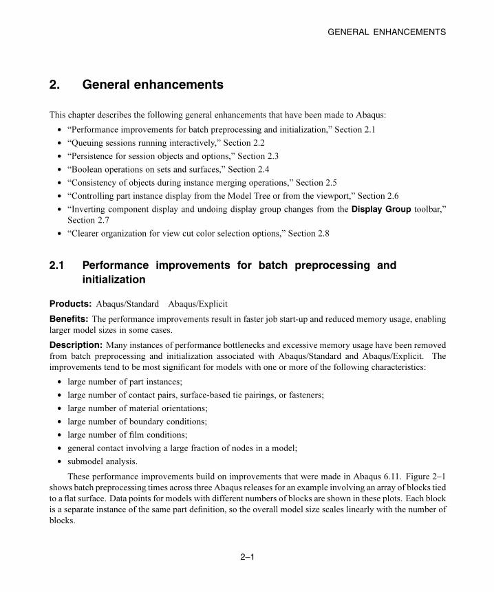
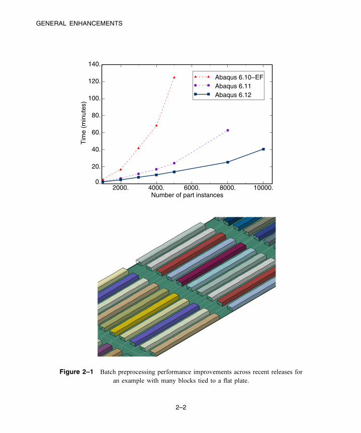
These performance improvements build on improvements that were made in Abaqus 6.11. Figure 2–1
shows batch preprocessing times across three Abaqus releases for an example involving an array of blocks tied
to a flat surface. Data points for models with different numbers of blocks are shown in these plots. Each block
is a separate instance of the same part definition, so the overall model size scales linearly with the number of
blocks.
2–1
Abaqus ID:
Printed on:
GENERAL ENHANCEMENTS
Number of part instances2000. 4000. 6000. 8000. 10000.
Tim
e (m
inut
es)
0.
20.
40.
60.
80.
100.
120.
140.
Abaqus 6.10−EFAbaqus 6.11Abaqus 6.12
Figure 2–1 Batch preprocessing performance improvements across recent releases for
an example with many blocks tied to a flat plate.
2–2
Abaqus ID:
Printed on:
GENERAL ENHANCEMENTS
The largest model considered has ten thousand blocks that are each modeled with one thousand
incompatible mode elements (element type C3D8I), such that the overall model has 170 million variables
(including internal degrees of freedom associated with C3D8I elements). As shown in Figure 2–1, the batch
preprocessing time has decreased significantly in recent releases, especially as the model size increases.
Data points are not shown for the largest models in previous releases because memory limits were reached
during batch preprocessing in these cases. Memory usage reductions enable these models to run successfully
with Abaqus 6.12.
2.2 Queuing sessions running interactively
Products: Abaqus/CAE Abaqus/Viewer
Benefits: You can now allow Abaqus/CAE or Abaqus/Viewer sessions running interactively to queue for a
license. Previously, only sessions running without the graphical user interface could be queued.
Description: You can use the new environment file variable lminteractivequeuing to indicate whether an
interactive Abaqus/CAE or Abaqus/Viewer session should queue for a license if one is not available. To allow
Abaqus/CAE or Abaqus/Viewer sessions running interactively to queue for a license, set this parameter equal
to ON. The default value is OFF.
References:
Abaqus Analysis User’s Manual
• “Using the Abaqus environment settings,” Section 3.3.1
Abaqus Installation and Licensing Guide
• “License management parameters,” Section 4.1.6
2.3 Persistence for session objects and options
Product: Abaqus/CAE
Benefits: By default, many objects and options that you specify in Abaqus/CAE persist only for the duration
of your session. You can now save these session objects and session options to a file so that you can use them
in subsequent sessions.
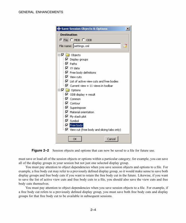
Description: Session objects and session options can now be saved to the model database, to an output
database, or to a settings file in XML format for use in subsequent sessions. Figure 2–2 shows the new SaveSession Objects & Options dialog box, which illustrates the types of objects and options that you can now
save. You can save or load categories of session objects and options individually; for example, you can choose
to retain all the display groups in your session but exclude any view cuts you have defined. However, you
2–3
Abaqus ID:
Printed on:
GENERAL ENHANCEMENTS
Figure 2–2 Session objects and options that can now be saved to a file for future use.
must save or load all of the session objects or options within a particular category; for example, you can save
all of the display groups in your session but not just one selected display group.
You must pay attention to object dependencies when you save session objects and options to a file. For
example, a free body cut may refer to a previously defined display group, so it would make sense to save both
display groups and free body cuts if you want to retain the free body cut in the future. Likewise, if you want
to save the list of active view cuts and free body cuts to a file, you should also save the view cuts and free
body cuts themselves.
You must pay attention to object dependencies when you save session objects to a file. For example, if
a free body cut refers to a previously defined display group, you must save both free body cuts and display
groups for that free body cut to be available in subsequent sessions.
2–4
Abaqus ID:
Printed on:
GENERAL ENHANCEMENTS
Abaqus/CAE Usage:All modules:
File→Save Session ObjectsFile→Load Session Objects
Reference:
Abaqus/CAE User’s Manual
• “Managing session objects and session options,” Section 9.9, in the online HTML version of this manual
2.4 Boolean operations on sets and surfaces
Product: Abaqus/CAE
Benefits: You can now use several Boolean operations to create new sets or surfaces from existing ones.
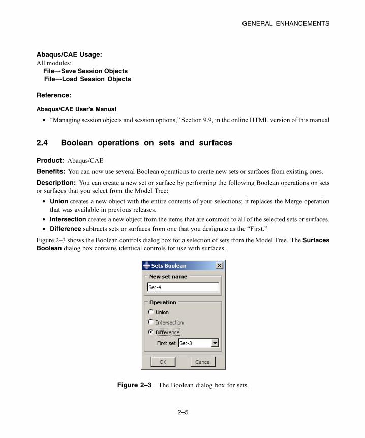
Description: You can create a new set or surface by performing the following Boolean operations on sets
or surfaces that you select from the Model Tree:
• Union creates a new object with the entire contents of your selections; it replaces the Merge operation
that was available in previous releases.
• Intersection creates a new object from the items that are common to all of the selected sets or surfaces.
• Difference subtracts sets or surfaces from one that you designate as the “First.”
Figure 2–3 shows the Boolean controls dialog box for a selection of sets from the Model Tree. The SurfacesBoolean dialog box contains identical controls for use with surfaces.
Figure 2–3 The Boolean dialog box for sets.
2–5
Abaqus ID:
Printed on:
GENERAL ENHANCEMENTS
Abaqus/CAE Usage:All modules:
Select multiple sets or surfaces from the Model Tree, then click mouse button 3 and select the Booleanoption from the menu.
Reference:
Abaqus/CAE User’s Manual
• “Performing Boolean operations on sets or surfaces,” Section 73.3.4, in the online HTML version of this
manual
2.5 Consistency of objects during instance merging operations
Product: Abaqus/CAE
Benefits: Several enhancements have been made to sets and surfaces resulting in consistent application of
loads, boundary conditions, and section assignments between geometry and mesh parts. Skin and stringer
reinforcements are also maintained.
Description: Merge operations for geometry objects have always preserved loads, boundary conditions, and
section assignments. Now when you merge mesh objects or create mesh parts, Abaqus/CAE copies, modifies,
or otherwise maintains the sets and surfaces in the model such that the loads, interactions, and other items are
preserved in the same way as they are for geometry.
When you create mesh parts from geometry, Abaqus/CAE copies and converts the contents of geometry
sets and surfaces as needed and applies them to mesh locations equivalent to the locations on the original
geometry. For example, vertices are converted to nodes, and edges are converted to a combination of nodes
and elements.
When you create a mesh part from assembly instances, you can choose to suppress the original
geometric instances and replace them with the new mesh part instance. The loads, boundary conditions,
section assignments, and reinforcements are all applied automatically to the mesh part through the converted
sets and surfaces. If you choose to switch back to the geometry, the sets and surfaces still contain the
geometric content (vertices, edges, and faces), so the loads, boundary conditions, etc. are still maintained.
Abaqus/CAE Usage:Mesh module:
Mesh→Create Mesh Part
Reference:
Abaqus/CAE User’s Manual
• “Creating a mesh part,” Section 17.20, in the online HTML version of this manual
2–6
Abaqus ID:
Printed on:
GENERAL ENHANCEMENTS
2.6 Controlling part instance display from the Model Tree or fromthe viewport
Product: Abaqus/CAE
Benefits: You can now control the display of part instances using new options in the Model Tree and in the
current viewport. This enhancement makes it easier to control the display of assemblies with a large number
of part instances.
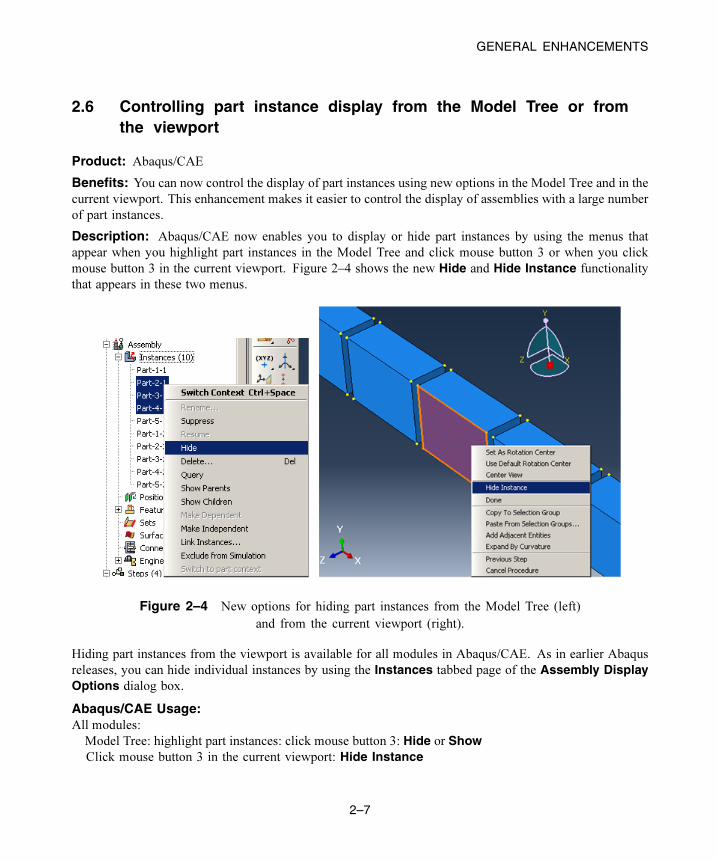
Description: Abaqus/CAE now enables you to display or hide part instances by using the menus that
appear when you highlight part instances in the Model Tree and click mouse button 3 or when you click
mouse button 3 in the current viewport. Figure 2–4 shows the new Hide and Hide Instance functionality
that appears in these two menus.
Figure 2–4 New options for hiding part instances from the Model Tree (left)
and from the current viewport (right).
Hiding part instances from the viewport is available for all modules in Abaqus/CAE. As in earlier Abaqus
releases, you can hide individual instances by using the Instances tabbed page of the Assembly DisplayOptions dialog box.
Abaqus/CAE Usage:All modules:
Model Tree: highlight part instances: click mouse button 3: Hide or ShowClick mouse button 3 in the current viewport: Hide Instance
2–7
Abaqus ID:
Printed on:
GENERAL ENHANCEMENTS
Reference:
Abaqus/CAE User’s Manual
• “Controlling instance visibility,” Section 76.14
2.7 Inverting component display and undoing display group changesfrom the Display Group toolbar
Product: Abaqus/CAE
Benefits: You can now invert the display of model components in the viewport with a single mouse click.
You can also undo or redo the changes you make to a display group directly from the Display Group toolbar.
These enhancements provide a quick shortcut for workflows that previously required several steps.
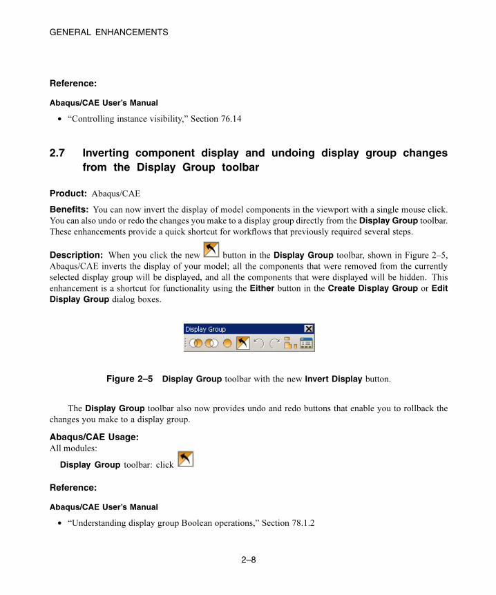
Description: When you click the new button in the Display Group toolbar, shown in Figure 2–5,
Abaqus/CAE inverts the display of your model; all the components that were removed from the currently
selected display group will be displayed, and all the components that were displayed will be hidden. This
enhancement is a shortcut for functionality using the Either button in the Create Display Group or EditDisplay Group dialog boxes.
Figure 2–5 Display Group toolbar with the new Invert Display button.
The Display Group toolbar also now provides undo and redo buttons that enable you to rollback the
changes you make to a display group.
Abaqus/CAE Usage:All modules:
Display Group toolbar: click
Reference:
Abaqus/CAE User’s Manual
• “Understanding display group Boolean operations,” Section 78.1.2
2–8
Abaqus ID:
Printed on:
GENERAL ENHANCEMENTS
2.8 Clearer organization for view cut color selection options
Product: Abaqus/CAE
Benefits: The View Cut Options dialog box now provides a clearer organization for the cap color selection
options.
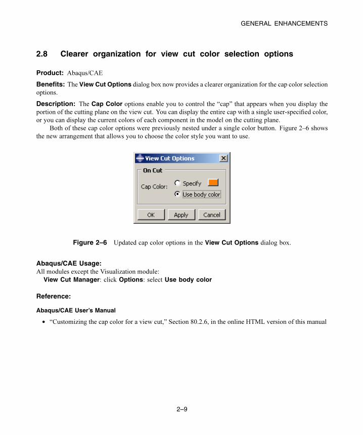
Description: The Cap Color options enable you to control the “cap” that appears when you display the
portion of the cutting plane on the view cut. You can display the entire cap with a single user-specified color,
or you can display the current colors of each component in the model on the cutting plane.
Both of these cap color options were previously nested under a single color button. Figure 2–6 shows
the new arrangement that allows you to choose the color style you want to use.
Figure 2–6 Updated cap color options in the View Cut Options dialog box.
Abaqus/CAE Usage:All modules except the Visualization module:
View Cut Manager: click Options: select Use body color
Reference:
Abaqus/CAE User’s Manual
• “Customizing the cap color for a view cut,” Section 80.2.6, in the online HTML version of this manual
2–9
Abaqus ID:
Printed on:

MODELING
3. Modeling
This chapter discusses features related to creating your model, such as node and element definition in
Abaqus/Standard, Abaqus/Explicit, and Abaqus/CFD; part and assembly definition in Abaqus/CAE;
importing and exporting models to or from Abaqus/CAE; and repairing problematic geometry. It provides
an overview of the following enhancements:
• “Modeling enhancements for electromagnetic analyses,” Section 3.1
• “SIMULIA Associative Interface for Abaqus/CAE,” Section 3.2
• “New naming convention for imported CAD parts,” Section 3.3
• “Retaining intersecting boundaries during part import from ACIS,” Section 3.4
• “Constraints in the Sketcher,” Section 3.5
• “Projecting mesh edges or nodes onto a sketch,” Section 3.6
• “Viewing model database attributes in the Visualization module,” Section 3.7
• “Creating geometry from orphan elements,” Section 3.8
• “Exporting contour plot data to 3D XML,” Section 3.9
• “Creating sets and surfaces during selection operations,” Section 3.10
• “Enhancements to mapped analytical fields in Abaqus/CAE,” Section 3.11
3.1 Modeling enhancements for electromagnetic analyses
Products: Abaqus/Standard Abaqus/CAE
Benefits: The addition of the electromagnetic model type attribute allows the Abaqus/CAE interface to
be tailored to perform an electromagnetic analysis in Abaqus/Standard. New features in several modules of
Abaqus/CAE allow the creation of electromagnetic parts and sections for electromagnetic analyses.
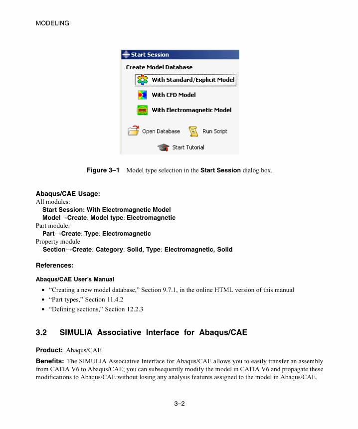
Description: When you create a model database, you can now select an electromagnetic model type to
specify that you are modeling an electromagnetic analysis (see “Time-harmonic electromagnetic analysis in
Abaqus/CAE,” Section 4.3). Most of the functionality presented in the Abaqus/CAE interface is filtered to
display only functionality that is valid for the electromagnetic model type. For example, mechanical loads
are not valid for an electromagnetic analysis; therefore, mechanical loads are not available in the load editor
when you specify the electromagnetic model type. Once a model database is created, you cannot change the
model type. Figure 3–1 shows the new model type selection available in the Start Session dialog box.
The new electromagnetic part type and section are available only in electromagnetic models.
Electromagnetic parts are used to define the domain for an eddy current analysis. You can define a
three-dimensional extruded, revolved, or swept part or a two-dimensional planar shell part. Electromagnetic
sections are used to define the properties of an electromagnetic part, including assigning material properties.
3–1
Abaqus ID:
Printed on:
MODELING
Figure 3–1 Model type selection in the Start Session dialog box.
Abaqus/CAE Usage:All modules:
Start Session: With Electromagnetic ModelModel→Create: Model type: Electromagnetic
Part module:
Part→Create: Type: ElectromagneticProperty module
Section→Create: Category: Solid, Type: Electromagnetic, Solid
References:
Abaqus/CAE User’s Manual
• “Creating a new model database,” Section 9.7.1, in the online HTML version of this manual
• “Part types,” Section 11.4.2
• “Defining sections,” Section 12.2.3
3.2 SIMULIA Associative Interface for Abaqus/CAE
Product: Abaqus/CAE
Benefits: The SIMULIA Associative Interface for Abaqus/CAE allows you to easily transfer an assembly
from CATIA V6 to Abaqus/CAE; you can subsequently modify the model in CATIA V6 and propagate these
modifications to Abaqus/CAE without losing any analysis features assigned to the model in Abaqus/CAE.
3–2
Abaqus ID:
Printed on:
MODELING
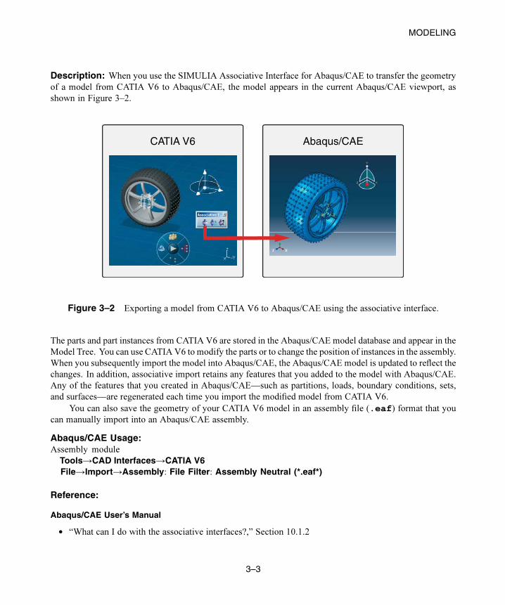
Description: When you use the SIMULIA Associative Interface for Abaqus/CAE to transfer the geometry
of a model from CATIA V6 to Abaqus/CAE, the model appears in the current Abaqus/CAE viewport, as
shown in Figure 3–2.
Abaqus/CAECATIA V6
Figure 3–2 Exporting a model from CATIA V6 to Abaqus/CAE using the associative interface.
The parts and part instances from CATIA V6 are stored in the Abaqus/CAE model database and appear in the
Model Tree. You can use CATIA V6 to modify the parts or to change the position of instances in the assembly.
When you subsequently import the model into Abaqus/CAE, the Abaqus/CAE model is updated to reflect the
changes. In addition, associative import retains any features that you added to the model with Abaqus/CAE.
Any of the features that you created in Abaqus/CAE—such as partitions, loads, boundary conditions, sets,
and surfaces—are regenerated each time you import the modified model from CATIA V6.
You can also save the geometry of your CATIA V6 model in an assembly file (.eaf) format that you
can manually import into an Abaqus/CAE assembly.
Abaqus/CAE Usage:Assembly module
Tools→CAD Interfaces→CATIA V6File→Import→Assembly: File Filter: Assembly Neutral (*.eaf*)
Reference:
Abaqus/CAE User’s Manual
• “What can I do with the associative interfaces?,” Section 10.1.2
3–3
Abaqus ID:
Printed on:
MODELING
3.3 New naming convention for imported CAD parts
Product: Abaqus/CAE
Benefits: When you import a part from an external-format file into a model, Abaqus/CAE now includes the
name of the CAD system from which the part originates in the feature name of the new part. This enhancement
provides more precise information about your model at a glance in the Model Tree.
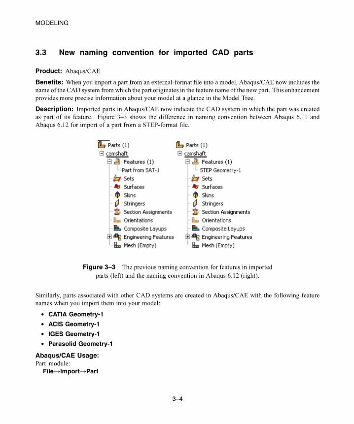
Description: Imported parts in Abaqus/CAE now indicate the CAD system in which the part was created
as part of its feature. Figure 3–3 shows the difference in naming convention between Abaqus 6.11 and
Abaqus 6.12 for import of a part from a STEP-format file.
Figure 3–3 The previous naming convention for features in imported
parts (left) and the naming convention in Abaqus 6.12 (right).
Similarly, parts associated with other CAD systems are created in Abaqus/CAE with the following feature
names when you import them into your model:
• CATIA Geometry-1
• ACIS Geometry-1
• IGES Geometry-1
• Parasolid Geometry-1
Abaqus/CAE Usage:Part module:
File→Import→Part
3–4
Abaqus ID:
Printed on:
MODELING
Reference:
Abaqus/CAE User’s Manual
• “Importing parts,” Section 10.7.2, in the online HTML version of this manual
3.4 Retaining intersecting boundaries during part import from ACIS
Product: Abaqus/CAE
Benefits: When you import solid parts from an ACIS file into Abaqus/CAE and combine them into a single
part, you can now retain the boundaries where the combined parts intersect. This enhancement can help you
eliminate invalid geometry for imported geometry.
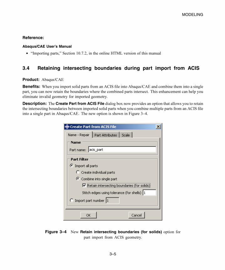
Description: The Create Part from ACIS File dialog box now provides an option that allows you to retain
the intersecting boundaries between imported solid parts when you combine multiple parts from an ACIS file
into a single part in Abaqus/CAE. The new option is shown in Figure 3–4.
Figure 3–4 New Retain intersecting boundaries (for solids) option for
part import from ACIS geometry.
3–5
Abaqus ID:
Printed on:
MODELING
Abaqus/CAE Usage:Part module:
File→Import→Part: Retain intersecting boundaries (for solids)
Reference:
Abaqus/CAE User’s Manual
• “Importing parts from an ACIS-format file,” Section 10.7.4, in the online HTML version of this manual
3.5 Constraints in the Sketcher
Product: Abaqus/CAE
Benefits: The constraint solver used to manage the addition of constraints and dimensions to a sketch has
been updated. This update affects constraint resolution in the Sketch module.
Description: The constraint solver used in the Sketcher for the last several releases has been replaced. The
new solver may show some different behavior in its solution of a desired constraint compared to the previous
one. When you are creating a new sketch for a part, these differences should be inconsequential. For example,
if you change the length dimension of a block, the new solver may adjust the right edge to achieve the desired
value, whereas the old one may have adjusted the left edge. When you upgrade a model that was created
in a previous Abaqus release, consider fully constraining your sketches in the old release first to avoid any
potential for changes.
If you have sketches that are generated via scripts, the generated entities should be identical to those
created in previous releases. However, their exact location may change due to the addition of constraints
using the new solver. If the commands in those scripts use indices, the scripts may execute without any
issues. However, you should check the sketch to ensure the desired solution. If those scripts use the findAt
scripting command to locate the generated entities and perform further operations, you may need to modify
the entities within the sketch so that they will be found by the command.
Abaqus/CAE Usage:Sketcher or Sketch module:
Add constraints or dimensions to an existing or new sketch
References:
Abaqus/CAE User’s Manual
• “Constraining, dimensioning, and parameterizing a sketch,” Section 20.12, in the online HTML version
of this manual
• “Translating Sketcher objects along a vector,” Section 20.16.1, in the online HTML version of this
manual
3–6
Abaqus ID:
Printed on:
MODELING
3.6 Projecting mesh edges or nodes onto a sketch
Product: Abaqus/CAE
Benefits: You can now project mesh edges or nodes onto a sketch when you add features to a mesh part.
This enhancement improves the sketching capabilities when you make changes to a mesh part.
Description: When you sketch the profile for a feature that you are adding to a mesh part, Abaqus/CAE now
enables you to project mesh edges and nodes onto the sketch sheet. The improved algorithm for projecting
mesh edges or nodes also allows you to project nodes and element edges as references.
Projected mesh edges are not constrained to the background because the mesh is transient. If you modify
or delete the mesh, the sketch does not regenerate after remeshing.
Abaqus/CAE Usage:Sketch module:
Add→References
References:
Abaqus/CAE User’s Manual
• “Adding reference geometry,” Section 20.14, in the online HTML version of this manual
• “Projecting edges onto a sketch,” Section 20.15, in the online HTML version of this manual
3.7 Viewing model database attributes in the Visualization module
Products: Abaqus/CAE Abaqus/Viewer
Benefits: You can now open a model database in the Visualization module and display and query data from
one of its models for a selected step. The ability to display the mesh, plot contours and symbols for model
data such as force or pressure loads, and probe model data can help you refine your model before submitting
an analysis.
Description: Abaqus/CAE now enables you to use the display and query functionality in the Visualization
module to examine data from one of the models in the current model database before you perform an analysis.
You can perform the following actions to investigate model data:
• Display the mesh.
• Display node and element labels.
• Plot contours or symbols of selected loads, predefined fields, or interactions.
• Probe the mesh or selected loads or predefined fields.
All models in the current model database are available for selection from the new Model Databasescontainer of the Results Tree. You can expand the container for an individual model database to display or
hide its part instances and to select the analysis step for which you want to investigate data. If you switch
3–7
Abaqus ID:
Printed on:
MODELING
to another module and modify the selected model, Abaqus/CAE automatically reflects those changes in the
Visualization module.
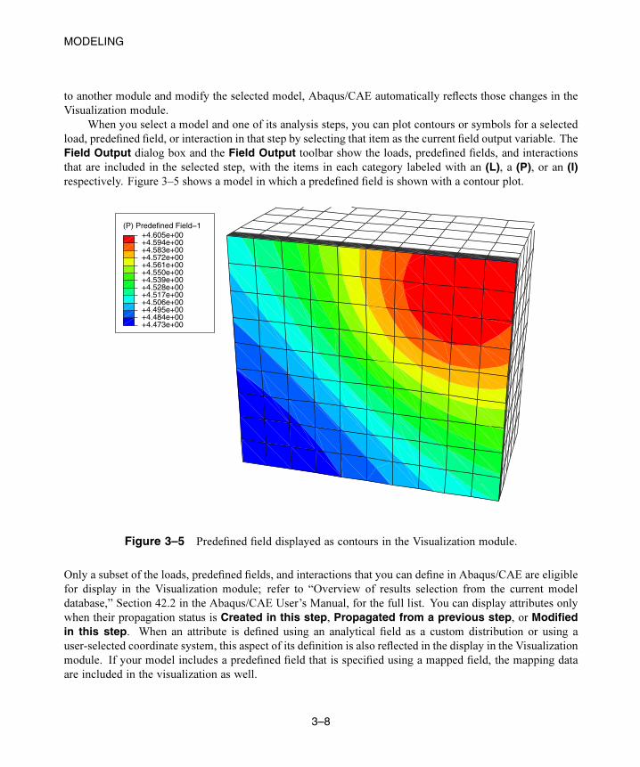
When you select a model and one of its analysis steps, you can plot contours or symbols for a selected
load, predefined field, or interaction in that step by selecting that item as the current field output variable. The
Field Output dialog box and the Field Output toolbar show the loads, predefined fields, and interactions
that are included in the selected step, with the items in each category labeled with an (L), a (P), or an (I)respectively. Figure 3–5 shows a model in which a predefined field is shown with a contour plot.
(P) Predefined Field−1
+4.473e+00+4.484e+00+4.495e+00+4.506e+00+4.517e+00+4.528e+00+4.539e+00+4.550e+00+4.561e+00+4.572e+00+4.583e+00+4.594e+00+4.605e+00
Figure 3–5 Predefined field displayed as contours in the Visualization module.
Only a subset of the loads, predefined fields, and interactions that you can define in Abaqus/CAE are eligible
for display in the Visualization module; refer to “Overview of results selection from the current model
database,” Section 42.2 in the Abaqus/CAE User’s Manual, for the full list. You can display attributes only
when their propagation status is Created in this step, Propagated from a previous step, or Modifiedin this step. When an attribute is defined using an analytical field as a custom distribution or using a
user-selected coordinate system, this aspect of its definition is also reflected in the display in the Visualization
module. If your model includes a predefined field that is specified using a mapped field, the mapping data
are included in the visualization as well.
3–8
Abaqus ID:
Printed on:
MODELING
You can also perform queries of your model in the Visualization module and probe for model data from
the current model database. Support for these options enables you to investigate aspects of your model such
as the composition of the mesh throughout the assembly or to retrieve the specific node where a particular
boundary condition is located.
When model data are displayed in the Visualization module, you can also color code the part instances
and adjust your display of part instances using display groups.
Abaqus/CAE Usage:Visualization module:
Results Tree: Model Databases: Model name
References:
Abaqus/CAE User’s Manual
• “Understanding the role of the Visualization module,” Section 40.1
• “Selecting the field output to display,” Section 42.5
3.8 Creating geometry from orphan elements
Product: Abaqus/CAE
Benefits: You can now use orphan element faces to create geometric faces and, in turn, entire parts.
Description: You can create geometric faces that follow the contour of orphan element faces. In addition to
selecting orphan element faces individually and by angle, you can use the following new selection methods
to choose orphan element faces from which to create new geometry:
• Limiting angle: Enter a maximum angle, and pick a starting element face; Abaqus/CAE measures the
angle from the selected face to each adjacent face. Selection continues outward from the picked face
until the measured angle with the original face is exceeded.
• Layer: Specify a number of layers, and pick a starting element face; Abaqus/CAE selects element faces
radiating out from one that you selected up to the number of layers. Selection continues until the number
of layers is reached or there are no more orphan element faces in a particular direction.
• Analytic: Pick a starting element face, and Abaqus/CAE adds all faces that it determines to be part of
the same analytic shape. Analytic shapes include planes, cylinders, cones, spheres, and tori.
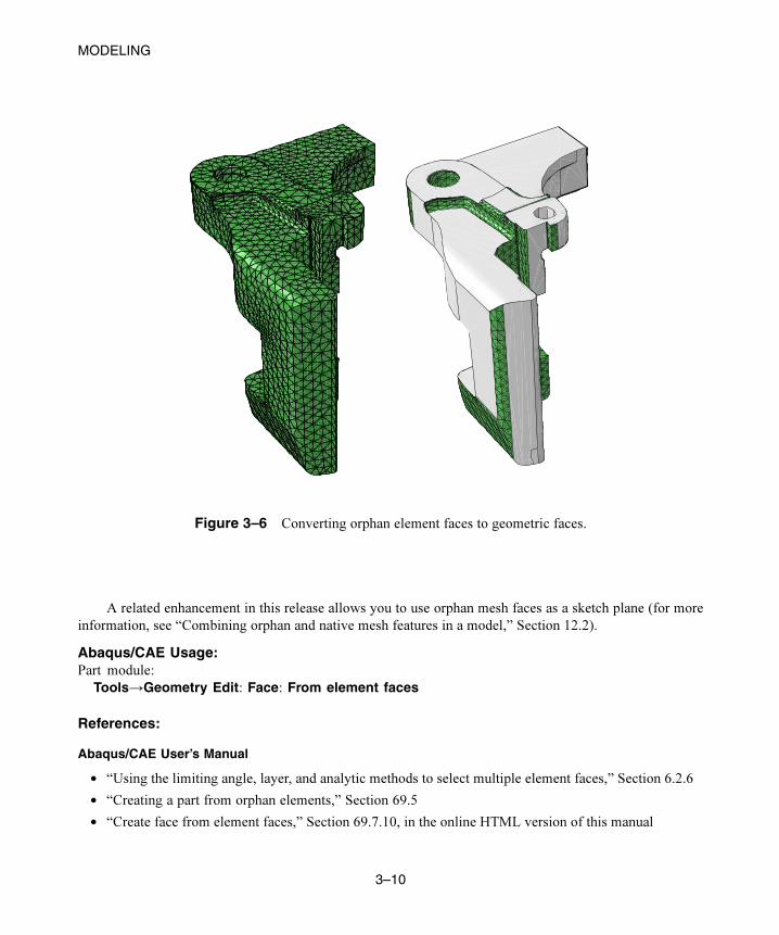
As you add faces, Abaqus/CAE stitches new faces to any existing geometry to produce a shell part. Figure 3–6
shows an orphan mesh part and the same part with most faces converted into geometry. When you are finished
creating new faces, you can use the other tools in the Geometry Edit toolset to repair the geometry if needed.
Each face is created as a separate feature, and you cannot edit the faces that you create from element faces.
However, you can add new geometry features, create a solid from the shell part, suppress or delete the orphan
mesh, and create a new mesh for the part.
3–9
Abaqus ID:
Printed on:
MODELING
Figure 3–6 Converting orphan element faces to geometric faces.
A related enhancement in this release allows you to use orphan mesh faces as a sketch plane (for more
information, see “Combining orphan and native mesh features in a model,” Section 12.2).
Abaqus/CAE Usage:Part module:
Tools→Geometry Edit: Face: From element faces
References:
Abaqus/CAE User’s Manual
• “Using the limiting angle, layer, and analytic methods to select multiple element faces,” Section 6.2.6
• “Creating a part from orphan elements,” Section 69.5
• “Create face from element faces,” Section 69.7.10, in the online HTML version of this manual
3–10
Abaqus ID:
Printed on:
MODELING
3.9 Exporting contour plot data to 3D XML
Product: Abaqus/CAE
Benefits: When exporting contour plot data in Abaqus/CAE to 3D XML-format files, texture mapping is
now used instead of tessellation, which reduces the size of the exported file.
Description: When you export three-dimensional model images of contour plots from Abaqus/CAE in
3D XML format, contour values are rendered using texture mapping. Texture mapping is a high-performance
rendering method that essentially lays an image of the contour values (the texture) over an image of the model.
Tessellation is a method of transforming arbitrary contour values into repeating patterns of distinct shapes,
such as triangles or simple polygons; the shape values are computed face by face. For overlay plots, contour
values are rendered using tessellation.
Abaqus/CAE Usage:All modules:
File→Export→3DXML
Reference:
Abaqus/CAE User’s Manual
• “Exporting viewport data to a 3D XML-format file,” Section 10.9.5, in the online HTML version of this
manual
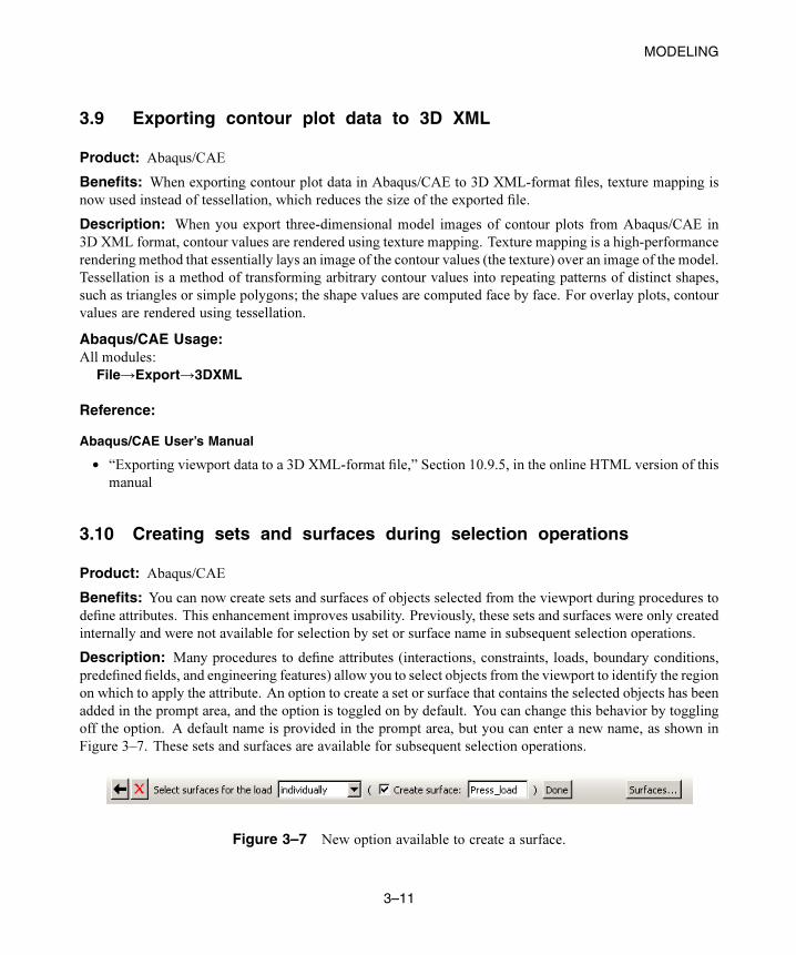
3.10 Creating sets and surfaces during selection operations
Product: Abaqus/CAE
Benefits: You can now create sets and surfaces of objects selected from the viewport during procedures to
define attributes. This enhancement improves usability. Previously, these sets and surfaces were only created
internally and were not available for selection by set or surface name in subsequent selection operations.
Description: Many procedures to define attributes (interactions, constraints, loads, boundary conditions,
predefined fields, and engineering features) allow you to select objects from the viewport to identify the region
on which to apply the attribute. An option to create a set or surface that contains the selected objects has been
added in the prompt area, and the option is toggled on by default. You can change this behavior by toggling
off the option. A default name is provided in the prompt area, but you can enter a new name, as shown in
Figure 3–7. These sets and surfaces are available for subsequent selection operations.
Figure 3–7 New option available to create a surface.
3–11
Abaqus ID:
Printed on:
MODELING
Abaqus/CAE Usage:Interaction module and Load module:
Various procedures: Toggle on Create set or Create surface, and specify name in the prompt area
Reference:
Abaqus/CAE User’s Manual
• “What objects can you select from the viewport?,” Section 6.1.1
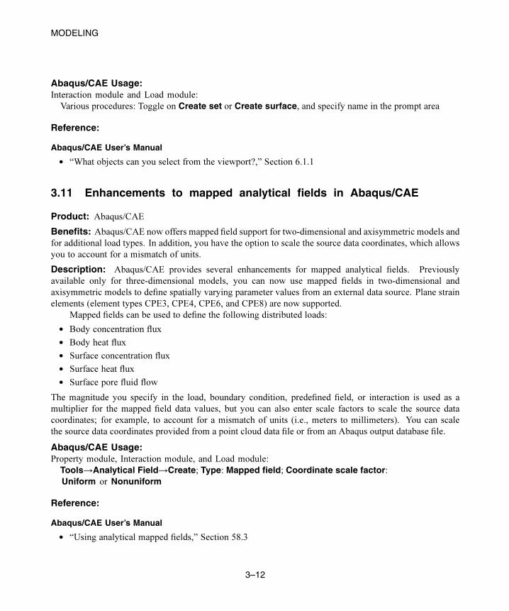
3.11 Enhancements to mapped analytical fields in Abaqus/CAE
Product: Abaqus/CAE
Benefits: Abaqus/CAE now offers mapped field support for two-dimensional and axisymmetric models and
for additional load types. In addition, you have the option to scale the source data coordinates, which allows
you to account for a mismatch of units.
Description: Abaqus/CAE provides several enhancements for mapped analytical fields. Previously
available only for three-dimensional models, you can now use mapped fields in two-dimensional and
axisymmetric models to define spatially varying parameter values from an external data source. Plane strain
elements (element types CPE3, CPE4, CPE6, and CPE8) are now supported.
Mapped fields can be used to define the following distributed loads:
• Body concentration flux
• Body heat flux
• Surface concentration flux
• Surface heat flux
• Surface pore fluid flow
The magnitude you specify in the load, boundary condition, predefined field, or interaction is used as a
multiplier for the mapped field data values, but you can also enter scale factors to scale the source data
coordinates; for example, to account for a mismatch of units (i.e., meters to millimeters). You can scale
the source data coordinates provided from a point cloud data file or from an Abaqus output database file.
Abaqus/CAE Usage:Property module, Interaction module, and Load module:
Tools→Analytical Field→Create; Type: Mapped field; Coordinate scale factor:Uniform or Nonuniform
Reference:
Abaqus/CAE User’s Manual
• “Using analytical mapped fields,” Section 58.3
3–12
Abaqus ID:
Printed on:
ANALYSIS PROCEDURES
4. Analysis procedures
This chapter discusses features related to defining an analysis. It provides an overview of the following
enhancements:
Fluid analysis
• “Implicit advection in Abaqus/CFD,” Section 4.1
• “Porous media flows in Abaqus/CFD,” Section 4.2
Electromagnetic analysis
• “Time-harmonic electromagnetic analysis in Abaqus/CAE,” Section 4.3
• “Coupled thermal-electrical-structural analysis in Abaqus/CAE,” Section 4.4
• “Magnetostatic analysis in Abaqus/Standard,” Section 4.5
• “Transient eddy current analysis in Abaqus/Standard,” Section 4.6
4.1 Implicit advection in Abaqus/CFD
Products: Abaqus/CFD Abaqus/CAE
Benefits: Implicit treatment of advection or the convective transport terms helps in achieving larger stable
time steps in Abaqus/CFD simulations. The implicit treatment relaxes the mesh size–dependent Courant-
Freidrichs-Levy (CFL) condition on the stable time step size. The CFL condition for explicit advective
schemes can be too restrictive for steady-state analyses involving thin boundary layer meshes. This feature
is especially useful for marching quickly toward a steady-state solution, reducing simulation time by a factor
of 10 or more.
Description: Explicit treatment of advection terms requires that the CFL stability condition be respected;
i.e., CFL . Implicit advection admits a larger CFL condition (CFL ).
Abaqus/CAE Usage:Step module:
Step→Create: General: Flow; Incrementation tabbed page: Advection time integration parameters
References:
Abaqus Analysis User’s Manual
• “Time incrementation” in “Incompressible fluid dynamic analysis,” Section 6.6.2
Abaqus/CAE User’s Manual
• “Configuring a flow procedure” in “Configuring general analysis procedures,” Section 14.11.1, in the
online HTML version of this manual
4–1
Abaqus ID:
Printed on:
ANALYSIS PROCEDURES
Abaqus Keywords Reference Manual
• *CFD
4.2 Porous media flows in Abaqus/CFD
Products: Abaqus/CFD Abaqus/CAE
Benefits: Flows through fluid-saturated porous media occur in a wide range of industrial and environmental
applications. Examples include packed-bed heat exchangers, heat pipes, thermal insulation, petroleum
reservoirs, nuclear waste repositories, geothermal engineering, thermal management of electronic devices,
metal alloy casting, and flow past porous scaffolds in bioreactors. The new enhancement is very useful for
simulating such flows. Flows with or without heat transfer are supported both in pure porous medium and
conjugate domains containing both porous and pure fluid regions.
Description: For isothermal flows in porous media, the model implemented in Abaqus/CFD is based on
the volume-averaged Darcy-Brinkman-Forchheimer equations that account for both Darcian and inertial non-
Darcian effects. The following assumptions are made in deriving the governing equations:
• The porosity of the medium does not vary with time or the time scale of variation of the porosity is
considered to be much larger than the dominant time scales of the fluid motion.
• The permeability of the porous medium is isotropic and dependent only on the porosity of the medium.
The widely used Carman-Kozeny permeability-porosity relationship is included in the enhancement.
The porous drag forces (namely, the Darcy and Forchheimer drag forces) are activated for a prescribed element
set by specifying them as distributed loads. For more information, see “New porous drag body force load in
Abaqus/CFD,” Section 8.8.
For porous flows with heat transfer, the volume-averaged temperature transport equation is considered
with the assumption of local thermal equilibrium. You define a fluid section for heat transfer analysis involving
porous media.
Abaqus/CAE Usage:Property module:
Material editor: Other→Pore Fluid→Permeability: Type: Isotropic (CFD) or Carman-KozenySection→Create: Category: Fluid, Type: Porous
References:
Abaqus Analysis User’s Manual
• “Porous media flows” in “Incompressible fluid dynamic analysis,” Section 6.6.2
• “Permeability,” Section 26.6.2
• “Fluid element library,” Section 28.2.2
4–2
Abaqus ID:
Printed on:
ANALYSIS PROCEDURES
Abaqus/CAE User’s Manual
• “Defining isotropic permeability in anAbaqus/CFD analysis” in “Defining a fluid-filled porous material,”
Section 12.12.3, in the online HTML version of this manual
• “Defining permeability based on the Carman-Kozeny relation” in “Defining a fluid-filled porous
material,” Section 12.12.3, in the online HTML version of this manual
• “Creating fluid sections for porous media,” Section 12.13.14, in the online HTML version of this manual
Abaqus Keywords Reference Manual
• *DLOAD
• *FLUID SECTION
• *PERMEABILITY
4.3 Time-harmonic electromagnetic analysis in Abaqus/CAE
Products: Abaqus/Standard Abaqus/CAE
Benefits: You can now perform a time-harmonic electromagnetic analysis that accounts for full coupling
between electric and magnetic fields in Abaqus/CAE, which increases the coverage of Abaqus product
functionality.
Description: Abaqus/CAE now supports Abaqus/Standard time-harmonic electromagnetic (eddy current)
analyses to calculate the eddy currents that are induced in a conductor placed within a time-harmonic magnetic
field. You specify one or more excitation frequencies, one or more frequency ranges, or a combination of
excitation frequencies and ranges to obtain the time-harmonic solution directly at a given excitation frequency.
Abaqus/CAE Usage:Step module:
Step→Create: Linear perturbation: Electromagnetic, Time harmonic
References:
Abaqus Analysis User’s Manual
• “Eddy current analysis,” Section 6.7.5
Abaqus/CAE User’s Manual
• “Configuring a time-harmonic electromagnetic analysis” in “Configuring linear perturbation analysis
procedures,” Section 14.11.2, in the online HTML version of this manual
4–3
Abaqus ID:
Printed on:
ANALYSIS PROCEDURES
4.4 Coupled thermal-electrical-structural analysis in Abaqus/CAE
Products: Abaqus/Standard Abaqus/CAE
Benefits: You can now perform a coupled thermal-electrical-structural analysis in Abaqus/CAE, which
increases the coverage of Abaqus product functionality.
Description: Abaqus/CAE now supports Abaqus/Standard analyses that fully couple the effects of a
simultaneous heat transfer, electrical, and structural procedure. A fully coupled thermal-electrical-structural
analysis is the union of a coupled thermal-displacement analysis and a coupled thermal-electrical analysis.
Coupling between the temperature and electrical degrees of freedom arises from temperature-dependent
electrical conductivity and internal heat generation (Joule heating), which is a function of the electrical current
density. Coupling between the temperature and displacement degrees of freedom arises from temperature-
dependent material properties, thermal expansion, and internal heat generation, which is a function of inelastic
deformation of the material. Coupling between the electrical and displacement degrees of freedom arises in
problems where electricity flows between contact surfaces.
Abaqus/CAE Usage:Step module:
Step→Create: General: Coupled thermal-electric-structural
References:
Abaqus Analysis User’s Manual
• “Fully coupled thermal-electrical-structural analysis,” Section 6.7.4
Abaqus/CAE User’s Manual
• “Configuring a fully coupled, simultaneous heat transfer, electrical, and structural procedure” in
“Configuring general analysis procedures,” Section 14.11.1, in the online HTML version of this manual
4.5 Magnetostatic analysis in Abaqus/Standard
Product: Abaqus/Standard
Benefits: You can now perform a magnetostatic analysis that computes the magnetic field due to a known
distribution of direct current.
Description: The magnetostatic approximation to Maxwell’s equations describing electromagnetic
phenomena is solved to compute the magnetic field due to a known distribution of direct current. The
magnetic field is completely decoupled from the electric field; as a result, the electric field does not enter
the magnetostatic formulation. Magnetostatic analysis is available with two-dimensional (planar) and
three-dimensional continuum elements and is based on an element edge-based interpolation of fields instead
of the usual node-based interpolation. The magnetostatic analysis can be driven by prescribed volume and/or
surface current density vectors or by prescribed values of the magnetic vector potential on surfaces. The
4–4
Abaqus ID:
Printed on:
ANALYSIS PROCEDURES
magnetic behavior of the medium can be linear or nonlinear and must be defined everywhere in the domain.
Nonlinear magnetic behavior can be defined in terms of one or more B–H curves.
References:
Abaqus Analysis User’s Manual
• “Electromagnetic analysis procedures,” Section 6.7.1
• “Magnetostatic analysis,” Section 6.7.6
• “Magnetic permeability,” Section 26.5.3
• “Two-dimensional solid element library,” Section 28.1.3
• “Three-dimensional solid element library,” Section 28.1.4
Abaqus Keywords Reference Manual
• *D EM POTENTIAL
• *DECURRENT
• *DSECURRENT
• *MAGNETIC PERMEABILITY
• *MAGNETOSTATIC
• *NONLINEAR BH
Abaqus User Subroutines Reference Manual
• “UDECURRENT,” Section 1.1.23
• “UDEMPOTENTIAL,” Section 1.1.24
• “UDSECURRENT,” Section 1.1.26
Abaqus Verification Manual
• “Magnetostatic analysis,” Section 3.6.2
4.6 Transient eddy current analysis in Abaqus/Standard
Product: Abaqus/Standard
Benefits: You can now perform a transient eddy current analysis that accounts for full coupling between the
electric and magnetic fields.
Description: You can now calculate the eddy currents that are induced in a conductor placed within a
time-varying magnetic field. The magnetic field can be generated by a coil carrying a time-varying current,
or it can be specified directly by means of appropriate boundary conditions/loads. The solution procedure is
based on obtaining a transient solution to Maxwell’s equations describing electromagnetic phenomena under
the low-frequency assumption and, hence, accounts for strong coupling between the electric and the magnetic
4–5
Abaqus ID:
Printed on:
ANALYSIS PROCEDURES
fields. Transient eddy current analysis is available with two-dimensional (planar) and three-dimensional
continuum elements and is based on an element edge-based interpolation of fields instead of the usual node-
based interpolation. The transient eddy current analysis can be driven by prescribed volume and/or surface
current density vectors or by prescribed values of the magnetic vector potential on surfaces. The magnetic
behavior of the medium can be linear or nonlinear and must be defined everywhere in the domain. Nonlinear
magnetic behavior can be defined in terms of one or more B–H curves. Electrical conductivity must be defined
in the conductor regions.
References:
Abaqus Analysis User’s Manual
• “Electromagnetic analysis procedures,” Section 6.7.1
• “Eddy current analysis,” Section 6.7.5
• “Magnetic permeability,” Section 26.5.3
• “Two-dimensional solid element library,” Section 28.1.3
• “Three-dimensional solid element library,” Section 28.1.4
Abaqus Keywords Reference Manual
• *D EM POTENTIAL
• *DECURRENT
• *DSECURRENT
• *ELECTROMAGNETIC
• *MAGNETIC PERMEABILITY
• *NONLINEAR BH
Abaqus User Subroutines Reference Manual
• “UDECURRENT,” Section 1.1.23
• “UDEMPOTENTIAL,” Section 1.1.24
• “UDSECURRENT,” Section 1.1.26
Abaqus Verification Manual
• “Eddy current analysis,” Section 3.6.1
4–6
Abaqus ID:
Printed on:
ANALYSIS TECHNIQUES
5. Analysis techniques
This chapter discusses features related to analysis techniques in Abaqus. It provides an overview of the
following enhancements:
Substructuring
• “Substructure generation using the AMS eigensolver,” Section 5.1
Matrix generation
• “Matrix functionality enhancements,” Section 5.2
Modeling discontinuities
• “Enhancements to the XFEM-based crack propagation capability,” Section 5.3
Fracture mechanics
• “Enhancements to the Virtual Crack Closure Technique (VCCT),” Section 5.4
Eulerian analysis
• “Adaptive mesh refinement for an Eulerian mesh,” Section 5.5
Particle methods
• “Smoothed particle hydrodynamics improvements,” Section 5.6
5.1 Substructure generation using the AMS eigensolver
Products: Abaqus/Standard Abaqus/AMS
Benefits: A new innovative algorithm generating a substructure using the AMS eigensolver significantly
improves substructure generation performance. This new algorithm also eliminates the requirement of full
eigenmodes recovery for the substructure generation step; therefore, disk space usage in the substructure
generation step can be reduced significantly if eigenmodes are recovered only at the user-defined node set.
Description: A new substructure generation capability in the AMS eigensolver delivers significant
performance improvement and reduces disk space requirements for substructure generation.
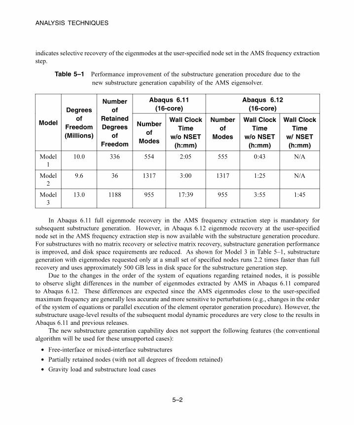
Table 5–1 illustrates the improved substructure generation performance. This example includes an
AMS frequency extraction step and the subsequent substructure generation step on a system with Intel
Westmere processors and 128 GB physical memory for three industrial models: Model 1 is an 10 million
degree of freedom automotive body-in-white model with full substructure matrix recovery, Model 2 is a
9.6 million degree of freedom automotive vehicle body model with full substructure matrix recovery, and
Model 3 is a 13 million degree of freedom powertrain model with no substructure matrix recovery. In the
table “w/o NSET” indicates full eigenmodes recovery in the AMS frequency extraction step and “w/ NSET”
5–1
Abaqus ID:
Printed on:
ANALYSIS TECHNIQUES
indicates selective recovery of the eigenmodes at the user-specified node set in the AMS frequency extraction
step.
Table 5–1 Performance improvement of the substructure generation procedure due to the
new substructure generation capability of the AMS eigensolver.
Abaqus 6.11(16-core)
Abaqus 6.12(16-core)
Model
Degreesof
Freedom(Millions)
Numberof
RetainedDegrees
ofFreedom
Numberof
Modes
Wall ClockTime
w/o NSET(h:mm)
Numberof
Modes
Wall ClockTime
w/o NSET(h:mm)
Wall ClockTime
w/ NSET(h:mm)
Model
1
10.0 336 554 2:05 555 0:43 N/A
Model
2
9.6 36 1317 3:00 1317 1:25 N/A
Model
3
13.0 1188 955 17:39 955 3:55 1:45
In Abaqus 6.11 full eigenmode recovery in the AMS frequency extraction step is mandatory for
subsequent substructure generation. However, in Abaqus 6.12 eigenmode recovery at the user-specified
node set in the AMS frequency extraction step is now available with the substructure generation procedure.
For substructures with no matrix recovery or selective matrix recovery, substructure generation performance
is improved, and disk space requirements are reduced. As shown for Model 3 in Table 5–1, substructure
generation with eigenmodes requested only at a small set of specified nodes runs 2.2 times faster than full
recovery and uses approximately 500 GB less in disk space for the substructure generation step.
Due to the changes in the order of the system of equations regarding retained nodes, it is possible
to observe slight differences in the number of eigenmodes extracted by AMS in Abaqus 6.11 compared
to Abaqus 6.12. These differences are expected since the AMS eigenmodes close to the user-specified
maximum frequency are generally less accurate and more sensitive to perturbations (e.g., changes in the order
of the system of equations or parallel execution of the element operator generation procedure). However, the
substructure usage-level results of the subsequent modal dynamic procedures are very close to the results in
Abaqus 6.11 and previous releases.
The new substructure generation capability does not support the following features (the conventional
algorithm will be used for these unsupported cases):
• Free-interface or mixed-interface substructures
• Partially retained nodes (with not all degrees of freedom retained)
• Gravity load and substructure load cases
5–2
Abaqus ID:
Printed on:
ANALYSIS TECHNIQUES
• Coupled acoustic-structural substructure
• Unsymmetric substructures
References:
Abaqus Analysis User’s Manual
• “Natural frequency extraction,” Section 6.3.5
• “Defining substructures,” Section 10.1.2
Abaqus Keywords Reference Manual
• *FREQUENCY
• *SUBSTRUCTURE GENERATE
5.2 Matrix functionality enhancements
Product: Abaqus/Standard
Benefits: Enhancements to matrix generation and to the matrix usage functionality significantly improve
the usability of matrix modeling techniques.
Description: The matrix generation procedure has been enhanced to allow you to specify “public nodes”
that will be visible in the matrix usage model; all other nodes are designated as internal nodes and effectively
hidden in the matrix usage model. By specifying public nodes, you can reduce the number of user-defined
nodes in the matrix usage model, which simplifies the new remapping process (described below).
The behavior for writing generated global matrices has been changed. By default, matrices are generated
in the matrix input text format, which now retains negative node numbers for internal nodes; previously,
internal node labels were converted into large positive numbers. If matrices are generated in the text labeling
format, internal node labels are now converted into large positive numbers; previously, internal node labels
were not converted when using this format. The matrix usage functionality has been enhanced to allow using
matrices with negative node labels for the Abaqus internal nodes.
User-defined matrix nodes specified as public nodes can be remapped (renamed) to different node labels
in the matrix usage model. This new remapping feature allows you to use several instances of the same matrix,
and it makes the matrix usage functionality similar to using substructures.
References:
Abaqus Analysis User’s Manual
• “Defining matrices,” Section 2.11.1
• “Generating matrices,” Section 10.3.1
5–3
Abaqus ID:
Printed on:
ANALYSIS TECHNIQUES
Abaqus Keywords Reference Manual
• *MATRIX ASSEMBLE
• *MATRIX GENERATE
• *MATRIX INPUT
• *MATRIX OUTPUT
5.3 Enhancements to the XFEM-based crack propagation capability
Product: Abaqus/Standard
Benefits: The extended finite element method (XFEM) allows you to model discontinuities, such as cracks,
along an arbitrary, solution-dependent path during an analysis. This method can now be extended to support
axisymmetric elements and frictional contact between the cracked element surfaces. To reduce run time for
large analyses, full parallel execution of the element operations is now available.
Description: XFEM allows you to model crack growth without remeshing the crack surfaces since it does
not require the mesh to match the geometry of the crack. The XFEMmethod is extended to support first-order
axisymmetric elements. Up to 100 enrichment definitions can be specified in a model. The frictional stresses
can be included in the cracked element surfaces of an enriched element.
Parallel execution of the element operations is available through thread-based parallelization for analyses
with XFEM.
References:
Abaqus Analysis User’s Manual
• “Modeling discontinuities as an enriched feature using the extended finite element method,”
Section 10.7.1
Abaqus Keywords Reference Manual
• *BOUNDARY
• *ENRICHMENT
5.4 Enhancements to the Virtual Crack Closure Technique (VCCT)
Product: Abaqus/Standard
Benefits: The original Virtual Crack Closure Technique (VCCT) has been enhanced to allow the release of
multiple nodes in one increment and to allow the specification of different critical energies for the onset and
growth of a crack. This is very useful to effectively predict the delamination of composite structures and to
extend the VCCT capability to account for some ductile fracture resistance.
5–4
Abaqus ID:
Printed on:
ANALYSIS TECHNIQUES
Description: When the VCCT technique is used, crack propagation analysis is carried out on a nodal basis.
The crack-tip node debonds when the fracture criterion is reachedwithin a given tolerance. The time increment
will be cutback if the tolerance is exceeded. For an unstable crack growth problem, however, it is more
efficient to allow multiple nodes at and ahead of a crack tip to debond in one increment without cutting back
the increment size when the VCCT fracture criterion is satisfied. The original VCCT technique has been
enhanced to allow more nodes at and ahead of the crack tip to debond in one increment (rather than cutting
back the increment size until the fracture criterion is no longer satisfied for all the nodes ahead of the crack
tip). The forces at the debonded nodes are released completely immediately during the following increment.
The original VCCT criterion uses the principles of linear elastic fracture mechanics (LEFM). To account
for ductile resistance, you can specify two different critical fracture energy release rates: one for the onset of
a crack and the other for the growth of a crack with the reduction of the debonding force being governed by
a user-specified critical fracture energy release rate for crack growth.
References:
Abaqus Analysis User’s Manual
• “Crack propagation analysis,” Section 11.4.3
Abaqus Keywords Reference Manual
• *FRACTURE CRITERION
5.5 Adaptive mesh refinement for an Eulerian mesh
Product: Abaqus/Explicit
Benefits: You can now use the adaptive mesh refinement feature to locally increase the mesh resolution of
an Eulerian mesh during the analysis. This feature greatly increases the computational efficiency compared
to equivalent uniformly refined mesh.
Description: The adaptive mesh refinement feature automatically refines/coarsens elements in an Eulerian
domain based on the criteria you sepecify. You can select from a variety of refinement criteria to suit your
particular application. When applied to a shock propagation problem, this new feature can automatically
refine the elements around the moving shock front; the elements are also automatically coarsened once the
shock front passes. This feature is also very useful in problems where higher mesh resolution is needed to
more accurately capture the location of a material interface/contact surface.
References:
Abaqus Analysis User’s Manual
• “Defining adaptive mesh refinement in the Eulerian domain,” Section 14.1.4
5–5
Abaqus ID:
Printed on:
ANALYSIS TECHNIQUES
Abaqus Keywords Reference Manual
• *ADAPTIVE MESH REFINEMENT
5.6 Smoothed particle hydrodynamics improvements
Products: Abaqus/Explicit Abaqus/CAE
Benefits: You can now leverage the intrinsic strengths of Lagrangian finite elements and smoothed particle
hydrodynamic (SPH) methods when modeling a body. You can use finite elements to create the model and
allow these elements to convert to SPH particles during the analysis.
Description: For an analysis involving the conversion of continuum elements to SPH particles, you start
by defining a part as usual. You mesh the part with C3D8R, C3D6, or C3D4 reduced-integration elements or
a combination of these elements. You then specify that these “parent” elements are to convert to internally
generated SPH particles when a user-specified criterion is met. Gravity loads, contact interactions, initial
conditions, mass scaling, and output requests associated with the parent elements or nodes of the parent
elements will be transferred appropriately to the generated particles upon conversion.
By default, the smoothed particle hydrodynamic method implemented in Abaqus/Explicit uses a cubic
spline as the interpolation polynomial; quadratic and quintic interpolators are also available.
The implementation is based on the classical smoothed particle hydrodynamic theory. In addition, you
have the option of using a mean flow correction configuration update, commonly referred to in the literature
as the XSPH method, as well as a corrected first-order consistent kernel, referred to as the normalized SPH
(NSPH) method.
Abaqus/CAE Usage:Mesh module:
Mesh→Element Type: Conversion to particles: Yes
References:
Abaqus Analysis User’s Manual
• “Smoothed particle hydrodynamic analysis,” Section 15.1.1
• “Finite element conversion to SPH particles,” Section 15.1.2
• “Section controls,” Section 27.1.4
Abaqus/CAE User’s Manual
• “Element type assignment,” Section 17.5.3
Abaqus Keywords Reference Manual
• *DEPVAR
• *SECTION CONTROLS
5–6
Abaqus ID:
Printed on:
ANALYSIS TECHNIQUES
Abaqus Example Problems Manual
• “Impact of a water-filled bottle,” Section 2.3.2
Abaqus Verification Manual
• “Smoothed particle hydrodynamic analysis,” Section 3.20.1
5–7
Abaqus ID:
Printed on:

MATERIALS
6. Materials
This chapter discusses new material models or changes to existing material models. It provides an overview
of the following enhancements:
• “Material calibration for hyperelasticity with permanent set,” Section 6.1
• “Material models for electromagnetic problems in Abaqus/CAE,” Section 6.2
• “New electrical/magnetic material behavior category in material editor,” Section 6.3
• “Non-Newtonian viscosity in Abaqus/CFD,” Section 6.4
• “Enhancements to Mullins effect in Abaqus/Explicit,” Section 6.5
• “Viscoelasticity for cohesive elements with traction-separation behavior in Abaqus/Explicit,” Section 6.6
• “Rayleigh damping enhancement in Abaqus/Explicit,” Section 6.7
• “Parallel network viscoelastic model,” Section 6.8
• “Ductile damage initiation criterion enhancements in Abaqus/Explicit,” Section 6.9
• “Enhancements to creep models,” Section 6.10
• “Nonlinear magnetic behavior,” Section 6.11
6.1 Material calibration for hyperelasticity with permanent set
Product: Abaqus/CAE
Benefits: You can now derive hyperelasticity, plasticity, and Mullins effect material behaviors from
uniaxial and biaxial loading data sets in Abaqus/CAE and add these behaviors to a material definition. This
enhancement enables you to include more realistic material models of elastomers and thermoplastics in your
analysis.
Description: Abaqus/CAE now includes a third material calibration behavior, Hyperelasticity withpermanent set, that enables you to derive material behaviors for hyperelasticity, plasticity, and Mullins
effect from uniaxial and biaxial test data. When you select the data sets from which you want to derive these
material behaviors, Abaqus/CAE extracts each loading, unloading, and reloading component of the data as
well as the permanent set data and creates new calibration data sets for each cycle. This process enables you
to use a subset of these test data for the derivation of material behaviors.
Figure 6–1 shows the extracted data sets in theEdit Behavior dialog boxwith the first and fifth unloadingand reloading cycles toggled off. Data from these deselected cycles will not be included in the calculations
of material behaviors; and they are also excluded from the X–Y curves displayed in the viewport, as shown in
Figure 6–2.
6–1
Abaqus ID:
Printed on:
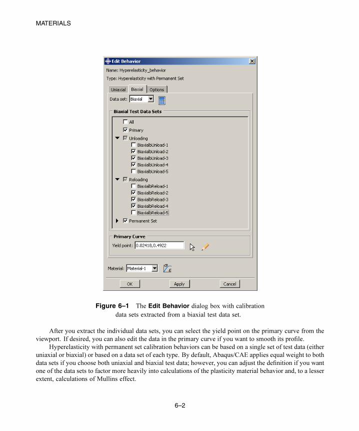
MATERIALS
Figure 6–1 The Edit Behavior dialog box with calibration
data sets extracted from a biaxial test data set.
After you extract the individual data sets, you can select the yield point on the primary curve from the
viewport. If desired, you can also edit the data in the primary curve if you want to smooth its profile.
Hyperelasticity with permanent set calibration behaviors can be based on a single set of test data (either
uniaxial or biaxial) or based on a data set of each type. By default, Abaqus/CAE applies equal weight to both
data sets if you choose both uniaxial and biaxial test data; however, you can adjust the definition if you want
one of the data sets to factor more heavily into calculations of the plasticity material behavior and, to a lesser
extent, calculations of Mullins effect.
6–2
Abaqus ID:
Printed on:
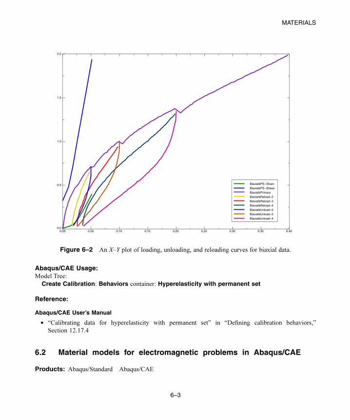
MATERIALS
0.00 0.05 0.10 0.15 0.20 0.25 0.30 0.35 0.400.0
0.5
1.0
1.5
2.0
BiaxialbPS−StrainBiaxialbPS−StressBiaxialbPrimaryBiaxialbReload−2BiaxialbReload−3BiaxialbReload−4BiaxialbUnload−2BiaxialbUnload−3BiaxialbUnload−4
Figure 6–2 An X–Y plot of loading, unloading, and reloading curves for biaxial data.
Abaqus/CAE Usage:Model Tree:
Create Calibration: Behaviors container: Hyperelasticity with permanent set
Reference:
Abaqus/CAE User’s Manual
• “Calibrating data for hyperelasticity with permanent set” in “Defining calibration behaviors,”
Section 12.17.4
6.2 Material models for electromagnetic problems in Abaqus/CAE
Products: Abaqus/Standard Abaqus/CAE
6–3
Abaqus ID:
Printed on:
MATERIALS
Benefits: Abaqus/CAE now supports material models for magnetic permeability and electrical conductivity
that allow you to carry out time-harmonic eddy current analyses.
Description: Abaqus/CAE supports electromagnetic capabilities to carry out time-harmonic eddy current
analyses (see “Time-harmonic electromagnetic analysis in Abaqus/CAE,” Section 4.3). You need to define
magnetic permeability everywhere in the domain and electrical conductivity in the conductor regions. The
material properties can be isotropic, orthotropic, or anisotropic and can also be defined to be frequency,
temperature, and/or field-variable dependent. Only linear magnetic and electrical behaviors can be modeled.
Abaqus/CAE Usage:Property module
Material editor: Electrical/Magnetic→Magnetic Permeability or Electrical Conductivity
References:
Abaqus/CAE User’s Manual
• “Defining electrical conductivity,” Section 12.11.1, in the online HTML version of this manual
• “Defining magnetic permeability,” Section 12.11.4, in the online HTML version of this manual
6.3 New electrical/magnetic material behavior category in materialeditor
Product: Abaqus/CAE
Benefits: The material editor reorganization categorizes the material behaviors to improve usability.
Description: With the addition of support for electromagnetic material models in Abaqus/CAE, the
Electrical/Magnetic material behavior category has been added to the material editor menus. Electrical
properties that were previously available from the Other→Electrical menu have been moved to the
Electrical/Magnetic menu, and the Magnetic Permeability behavior has been added, as shown in
Figure 6–3.
Abaqus/CAE Usage:Property module
Material editor: Electrical/Magnetic
Reference:
Abaqus/CAE User’s Manual
• “Defining electrical and magnetic material models,” Section 12.11, in the online HTML version of this
manual
6–4
Abaqus ID:
Printed on:
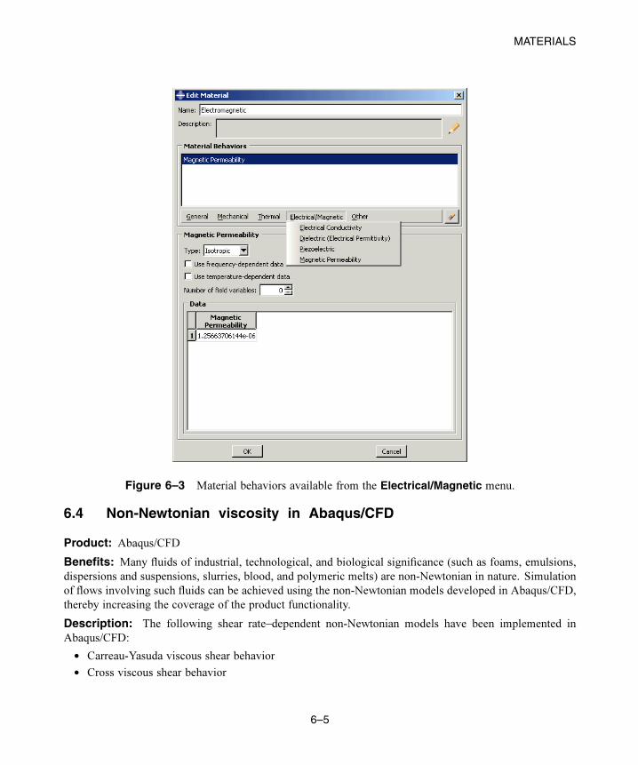
MATERIALS
Figure 6–3 Material behaviors available from the Electrical/Magnetic menu.
6.4 Non-Newtonian viscosity in Abaqus/CFD
Product: Abaqus/CFD
Benefits: Many fluids of industrial, technological, and biological significance (such as foams, emulsions,
dispersions and suspensions, slurries, blood, and polymeric melts) are non-Newtonian in nature. Simulation
of flows involving such fluids can be achieved using the non-Newtonian models developed in Abaqus/CFD,
thereby increasing the coverage of the product functionality.
Description: The following shear rate–dependent non-Newtonian models have been implemented in
Abaqus/CFD:
• Carreau-Yasuda viscous shear behavior
• Cross viscous shear behavior
6–5
Abaqus ID:
Printed on:
MATERIALS
• Ellis-Meter viscous shear behavior
• Herschel-Bulkley viscous shear behavior
• Powell-Eyring viscous shear behavior
• Power law viscous shear behavior
• Non-Newtonian viscous shear behavior in tabular form
References:
Abaqus Analysis User’s Manual
• “Viscosity,” Section 26.1.4
Abaqus Keywords Reference Manual
• *VISCOSITY
6.5 Enhancements to Mullins effect in Abaqus/Explicit
Products: Abaqus/Explicit Abaqus/CAE
Benefits: You can now define the damage behavior associated withMullins effect (stress softening of certain
filled elastomers) in Abaqus/Explicit with the new user subroutine VUMULLINS.
Description: User subroutine VUMULLINS is now available in Abaqus/Explicit to define the damage
behavior associated with Mullins effect in rubberlike materials and elastomeric foams. This feature provides
functionality equivalent to that of user subroutine UMULLINS previously available in Abaqus/Standard. The
subroutine provides users with access to solution-dependent state variables as well as temperature and field
variables. In addition to defining the damage variable, you can also define the strain energy dissipation due
to damage as well as a criterion for material failure and element deletion.
Abaqus/CAE Usage:Property module:
Material editor: Mechanical→Damage for Elastomers→Mullins Effect; Definition: User Defined
References:
Abaqus Analysis User’s Manual
• “Mullins effect,” Section 22.6.1
• “Energy dissipation in elastomeric foams,” Section 22.6.2
Abaqus/CAE User’s Manual
• “Mullins effect” in “Defining damage,” Section 12.9.3, in the online HTML version of this manual
6–6
Abaqus ID:
Printed on:
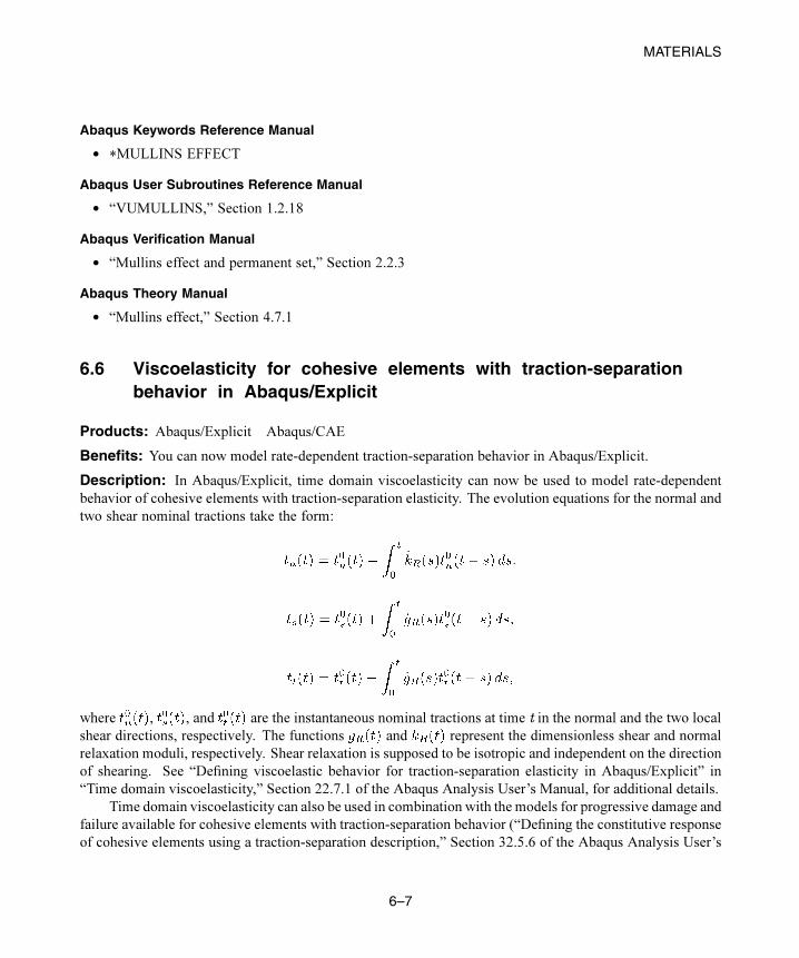
MATERIALS
Abaqus Keywords Reference Manual
• *MULLINS EFFECT
Abaqus User Subroutines Reference Manual
• “VUMULLINS,” Section 1.2.18
Abaqus Verification Manual
• “Mullins effect and permanent set,” Section 2.2.3
Abaqus Theory Manual
• “Mullins effect,” Section 4.7.1
6.6 Viscoelasticity for cohesive elements with traction-separationbehavior in Abaqus/Explicit
Products: Abaqus/Explicit Abaqus/CAE
Benefits: You can now model rate-dependent traction-separation behavior in Abaqus/Explicit.
Description: In Abaqus/Explicit, time domain viscoelasticity can now be used to model rate-dependent
behavior of cohesive elements with traction-separation elasticity. The evolution equations for the normal and
two shear nominal tractions take the form:
where , , and are the instantaneous nominal tractions at time t in the normal and the two local
shear directions, respectively. The functions and represent the dimensionless shear and normal
relaxation moduli, respectively. Shear relaxation is supposed to be isotropic and independent on the direction
of shearing. See “Defining viscoelastic behavior for traction-separation elasticity in Abaqus/Explicit” in
“Time domain viscoelasticity,” Section 22.7.1 of the Abaqus Analysis User’s Manual, for additional details.
Time domain viscoelasticity can also be used in combination with the models for progressive damage and
failure available for cohesive elements with traction-separation behavior (“Defining the constitutive response
of cohesive elements using a traction-separation description,” Section 32.5.6 of the Abaqus Analysis User’s
6–7
Abaqus ID:
Printed on:
MATERIALS
Manual). This combination allows modeling rate-dependent behavior both during the initial elastic response
(prior to damage initiation), as well as during damage progression.
Abaqus/CAE Usage:Property module:
Material editor: Mechanical→Elasticity→Viscoelastic; Domain: Time
References:
Abaqus Analysis User’s Manual
• “Defining viscoelastic behavior for traction-separation elasticity in Abaqus/Explicit” in “Time domain
viscoelasticity,” Section 22.7.1
• “Modeling rate-dependent traction-separation behavior in Abaqus/Explicit” in “Defining the constitutive
response of cohesive elements using a traction-separation description,” Section 32.5.6
Abaqus/CAE User’s Manual
• “Defining time domain viscoelasticity” in “Defining elasticity,” Section 12.9.1, in the online HTML
version of this manual
Abaqus Keywords Reference Manual
• *VISCOELASTIC
6.7 Rayleigh damping enhancement in Abaqus/Explicit
Products: Abaqus/Explicit Abaqus/CAE
Benefits: You can now specify temperature and/or field-dependent Rayleigh mass proportional and
stiffness proportional damping for all materials in Abaqus/Explicit. Mass proportional damping is now
allowed for ROTARYI and MASS elements in Abaqus/Explicit, which was previously supported only in
Abaqus/Standard.
Description: Abaqus/Explicit now allows you to define Rayleigh mass proportional and stiffness
proportional damping as a tabular function of temperature and/or field variables. In addition, mass
proportional damping is now allowed for ROTARYI and MASS elements in Abaqus/Explicit and can be
specified in Abaqus/CAE. This functionality was previously supported only in Abaqus/Standard.
Abaqus/CAE Usage:Property module or Interaction module:
Special→Inertia→Create: Point mass/inertia: Damping
6–8
Abaqus ID:
Printed on:
MATERIALS
References:
Abaqus Analysis User’s Manual
• “Material damping,” Section 26.1.1
• “Point masses,” Section 30.1.1
• “Rotary inertia,” Section 30.2.1
Abaqus/CAE User’s Manual
• “Defining point mass and rotary inertia,” Section 33.3, in the online HTML version of this manual
Abaqus Keywords Reference Manual
• *DAMPING
• *MASS
• *ROTARY INERTIA
Abaqus Verification Manual
• “Material damping in Abaqus/Explicit,” Section 2.2.31
• “Mass proportional damping in Abaqus/Explicit,” Section 2.2.32
6.8 Parallel network viscoelastic model
Product: Abaqus/Standard
Benefits: You can define nonlinear viscoelastic behavior with hyperelasticity using the new parallel network
viscoelastic model.
Description: The parallel network viscoelastic model allows realistic simulation of viscous materials that
may undergo large deformations, such as polymers. The model consists of multiple elastic and viscoelastic
networks as depicted in Figure 6–4. In the model one of the networks is purely elastic, and the remaining
networks are viscoelastic. The elastic response is specified using one of the hyperelastic material models,
and the viscous response is governed by a flow rule derived from the Mises stress potential and the strain-
hardening or the hyperbolic-sine evolution laws.
References:
Abaqus Analysis User’s Manual
• “Parallel network viscoelastic model,” Section 22.8.2
Abaqus Keywords Reference Manual
• *VISCOELASTIC
6–9
Abaqus ID:
Printed on:
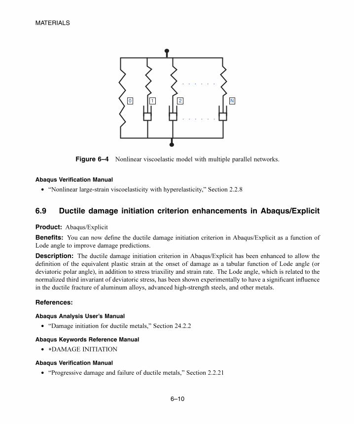
MATERIALS
. . . . . .
0 1 2 N
. . . . . .
Figure 6–4 Nonlinear viscoelastic model with multiple parallel networks.
Abaqus Verification Manual
• “Nonlinear large-strain viscoelasticity with hyperelasticity,” Section 2.2.8
6.9 Ductile damage initiation criterion enhancements in Abaqus/Explicit
Product: Abaqus/Explicit
Benefits: You can now define the ductile damage initiation criterion in Abaqus/Explicit as a function of
Lode angle to improve damage predictions.
Description: The ductile damage initiation criterion in Abaqus/Explicit has been enhanced to allow the
definition of the equivalent plastic strain at the onset of damage as a tabular function of Lode angle (or
deviatoric polar angle), in addition to stress triaxility and strain rate. The Lode angle, which is related to the
normalized third invariant of deviatoric stress, has been shown experimentally to have a significant influence
in the ductile fracture of aluminum alloys, advanced high-strength steels, and other metals.
References:
Abaqus Analysis User’s Manual
• “Damage initiation for ductile metals,” Section 24.2.2
Abaqus Keywords Reference Manual
• *DAMAGE INITIATION
Abaqus Verification Manual
• “Progressive damage and failure of ductile metals,” Section 2.2.21
6–10
Abaqus ID:
Printed on:
MATERIALS
6.10 Enhancements to creep models
Product: Abaqus/Standard
Benefits: Now you can specify whether total time or creep time should be used in creep models in which
time is used explicitly.
Description: In some of the creep models available in Abaqus/Standard, such as the time-hardening power
law model and the Singh-Mitchell model, time is used explicitly. Previously, the total time was used in these
models. Now, in addition to the total time, the creep time can be used as well. The creep time is computed as
the sum of the times of procedures with time-dependent material behavior. For the time-hardening power law
and Singh-Mitchell models, you can specify the time type. Similarly, for user-defined creep models either
the total or the creep time can be used. In this case both times are passed as parameters into user subroutine
CREEP.
References:
Abaqus Analysis User’s Manual
• “Rate-dependent plasticity: creep and swelling,” Section 23.2.4
• “Two-layer viscoplasticity,” Section 23.2.11
• “Extended Drucker-Prager models,” Section 23.3.1
• “Modified Drucker-Prager/Cap model,” Section 23.3.2
Abaqus Keywords Reference Manual
• *CAP CREEP
• *CREEP
• *DRUCKER PRAGER CREEP
• *VISCOUS
6.11 Nonlinear magnetic behavior
Product: Abaqus/Standard
Benefits: You can now specify nonlinear magnetic behavior of an electromagnetic medium through direct
specification of one or more B–H curves.
Description: The magnetic behavior of some electromagnetic media is characterized by a magnetic
permeability that strongly depends upon the strength of the magnetic field. Such nonlinear response is
typically described through one (for isotropic behavior) or three (for orthotropic behavior) B–H curves that
define, in tabular form, the strength of the magnetic flux density as a function of the strength of the magnetic
field. The model provided in Abaqus is suitable for modeling soft magnetic materials that show little or no
hysteresis.
6–11
Abaqus ID:
Printed on:
MATERIALS
References:
Abaqus Analysis User’s Manual
• “Eddy current analysis,” Section 6.7.5
• “Magnetostatic analysis,” Section 6.7.6
• “Magnetic permeability,” Section 26.5.3
Abaqus Keywords Reference Manual
• *MAGNETIC PERMEABILITY
• *NONLINEAR BH
6–12
Abaqus ID:
Printed on:
ELEMENTS
7. Elements
This chapter discusses elements available in Abaqus. It provides an overview of the following enhancements:
• “Support for electromagnetic elements in Abaqus/CAE,” Section 7.1
• “Unsymmetric storage for linear coupled stiffness and viscous damping for connections in
Abaqus/Standard,” Section 7.2
• “Thick-walled pipe elements in Abaqus/Standard,” Section 7.3
• “Defining the anisotropic mass tensor,” Section 7.4
7.1 Support for electromagnetic elements in Abaqus/CAE
Products: Abaqus/Standard Abaqus/CAE
Benefits: You can now assign element types from the electromagnetic family of elements to a solid region
of your model in Abaqus/CAE. This enhancement provides improved interactive meshing for the domain in
an electromagnetic analysis.
Description: The Element Type dialog box in the Mesh module now enables you to assign element types
from the electromagnetic family of elements to solid topologies in your model. The electromagnetic family
of Abaqus/Standard elements includes element types EMC2D3, EMC2D4, EMC3D4, and EMC3D8.
Abaqus/CAE Usage:Mesh module
Mesh→Element Type: Family: Electromagnetic
References:
Abaqus Analysis User’s Manual
• “Two-dimensional solid element library,” Section 28.1.3
• “Three-dimensional solid element library,” Section 28.1.4
Abaqus/CAE User’s Manual
• “Element type assignment,” Section 17.5.3
7.2 Unsymmetric storage for linear coupled stiffness and viscousdamping for connections in Abaqus/Standard
Product: Abaqus/Standard
7–1
Abaqus ID:
Printed on:
ELEMENTS
Benefits: A common modeling technique in the field of rotordynamics is to use unsymmetric stiffness and
damping matrices to model fluid film bearings supporting a rotating structure. Abaqus/Standard now supports
frequency-dependent unsymmetric linear coupled stiffness and viscous damping matrices to model fluid film
bearings in rotordynamic analyses.
Description: For the unsymmetric linear coupled stiffness case you define the spring stiffness matrix
components, , which are used in the equation
where is the force in the component of relative motion, is the motion of the component, and
is the coupling between the and components. For the unsymmetric linear coupled viscous damping
case you define the damping coefficient matrix components, , which are used in the equation
where is the force in the component of relative motion, is the velocity in the component, and
is the coupling between the and components.
References:
Abaqus Analysis User’s Manual
• “Connector elastic behavior,” Section 31.2.2
• “Connector damping behavior,” Section 31.2.3
Abaqus Keywords Reference Manual
• *CONNECTOR DAMPING
• *CONNECTOR ELASTICITY
7.3 Thick-walled pipe elements in Abaqus/Standard
Products: Abaqus/Standard Abaqus/CAE
Benefits: Abaqus/Standard now supports the modeling of thick-walled pipes, in which the hoop and radial
stress due to the applied pressure vary across the pipe cross-section. The thick-walled element formulation
better predicts the inelastic response under the effect of internal and external applied pressure for larger wall
thickness-to-radius ratios. In addition, the bending and torsional behavior is modeled more accurately without
recourse to thin-wall assumptions.
Description: Thick-walled pipe elements can be used in all general and linear perturbation procedures in
Abaqus/Standard that support displacement degrees of freedom. All pipe element load types are supported,
7–2
Abaqus ID:
Printed on:
ELEMENTS
as well as all pipe element material models with the exception of hyperelasticity. Thick-walled pipes have
radial stress as additional element output.
Abaqus/CAE Usage:Property module:
Profile→Create: Pipe: Thick walled
References:
Abaqus Analysis User’s Manual
• “Choosing a beam element,” Section 29.3.3
• “Beam cross-section library,” Section 29.3.9
Abaqus/CAE User’s Manual
• “Defining a pipe profile” in “Creating profiles,” Section 12.13.20, in the online HTML version of this
manual
Abaqus Keywords Reference Manual
• *BEAM SECTION
7.4 Defining the anisotropic mass tensor
Products: Abaqus/Standard Abaqus/Explicit Abaqus/CAE
Benefits: Abaqus/Standard and Abaqus/Explicit now allow for point masses to be anisotropic. This
enhancement is useful when you are modeling submerged structures where the influence of the surrounding
fluid is captured using “added mass” attached to the nodes of the structure. This modeling approximation
often results in an added mass that is direction dependent.
Description: You can now define an anisotropic point mass element by specifying the three principal values
and the principal directions. In a large-displacement analysis the local axes of the anisotropic mass rotate with
the rotation, if active, of the node to which the anisotropic mass is attached. The rotation degree of freedom
is active at a node if that node is connected to a beam, a conventional shell, a rotary inertia element, or a rigid
body. You can also specify mass proportional alpha damping and loads such as gravity for the anisotropic
point mass.
Abaqus/CAE Usage:Property or Interaction module:
Special→Inertia→Create: Point mass/inertia: select point: Magnitude: Anisotropic:, , and
7–3
Abaqus ID:
Printed on:
ELEMENTS
References:
Abaqus Analysis User’s Manual
• “Point masses,” Section 30.1.1
Abaqus/CAE User’s Manual
• “Defining point mass and rotary inertia,” Section 33.3, in the online HTML version of this manual
Abaqus Keywords Reference Manual
• *MASS
7–4
Abaqus ID:
Printed on:
PRESCRIBED CONDITIONS
8. Prescribed conditions
This chapter discusses loads, boundary conditions, and predefined fields. It provides an overview of the
following enhancements:
• “Prescribing loads and boundary conditions in an electromagnetic analysis in Abaqus/CAE,” Section 8.1
• “New category choices for loads and boundary conditions in Abaqus/CAE,” Section 8.2
• “Changing the coordinate system for fluid velocity boundary conditions in Abaqus/CAE,” Section 8.3
• “Enhancements to distributed body heat flux,” Section 8.4
• “Impedance conditions in modal steady-state dynamic analysis,” Section 8.5
• “Fluid cavity pressure predefined fields and boundary conditions in Abaqus/CAE,” Section 8.6
• “New rotordynamic load,” Section 8.7
• “New porous drag body force load in Abaqus/CFD,” Section 8.8
• “New passive outflow boundary type in Abaqus/CFD,” Section 8.9
• “Pressure boundary condition that varies with the total volume of fluid crossing a surface in
Abaqus/CFD,” Section 8.10
• “Base motion boundary conditions and PSD amplitudes in Abaqus/CAE,” Section 8.11
• “Total flux distribution option for surface heat flux in Abaqus/CAE,” Section 8.12
• “Defining connector loads and boundary conditions using assembled fasteners and template models,”
Section 8.13
8.1 Prescribing loads and boundary conditions in an electromagneticanalysis in Abaqus/CAE
Products: Abaqus/Standard Abaqus/CAE
Benefits: New electromagnetic loads and boundary conditions are available in Abaqus/CAE, which
increases the coverage of Abaqus product functionality.
Description: In Abaqus/CAE you can now define loads and boundary conditions for electromagnetic
analyses (see “Time-harmonic electromagnetic analysis in Abaqus/CAE,” Section 4.3). Time-harmonic eddy
current problems are usually driven by prescribed body or surface current densities in certain regions of the
model and require that you prescribe boundary conditions on surfaces. Both uniform and nonuniform loads
and boundary conditions can be prescribed.
8–1
Abaqus ID:
Printed on:
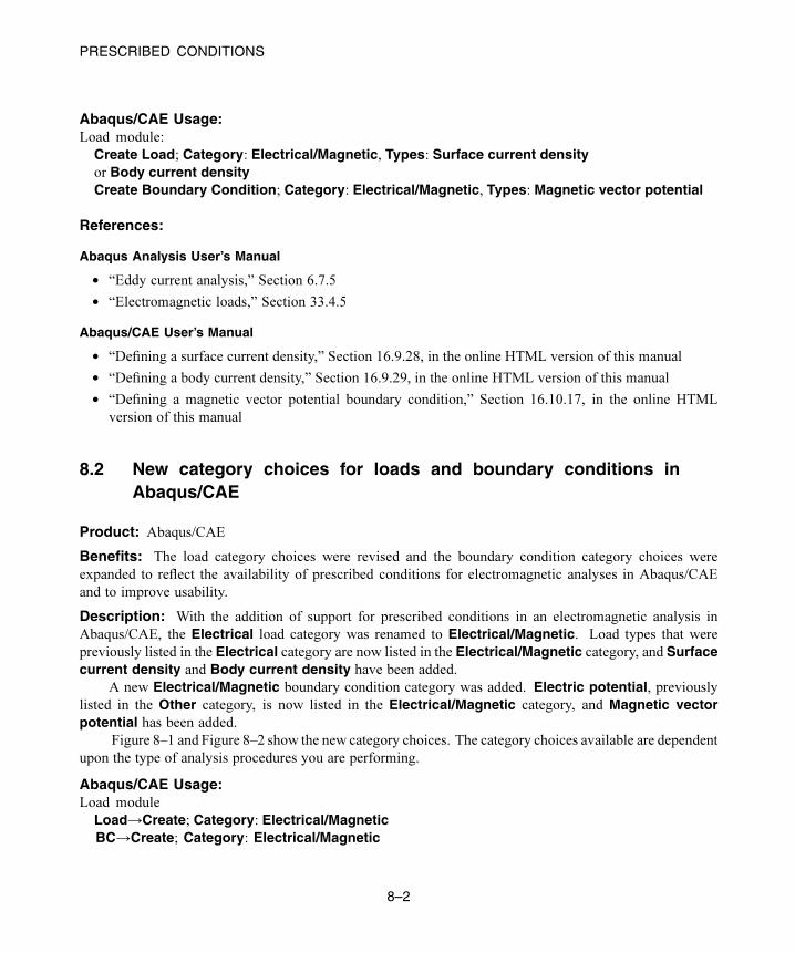
PRESCRIBED CONDITIONS
Abaqus/CAE Usage:Load module:
Create Load; Category: Electrical/Magnetic, Types: Surface current densityor Body current densityCreate Boundary Condition; Category: Electrical/Magnetic, Types: Magnetic vector potential
References:
Abaqus Analysis User’s Manual
• “Eddy current analysis,” Section 6.7.5
• “Electromagnetic loads,” Section 33.4.5
Abaqus/CAE User’s Manual
• “Defining a surface current density,” Section 16.9.28, in the online HTML version of this manual
• “Defining a body current density,” Section 16.9.29, in the online HTML version of this manual
• “Defining a magnetic vector potential boundary condition,” Section 16.10.17, in the online HTML
version of this manual
8.2 New category choices for loads and boundary conditions inAbaqus/CAE
Product: Abaqus/CAE
Benefits: The load category choices were revised and the boundary condition category choices were
expanded to reflect the availability of prescribed conditions for electromagnetic analyses in Abaqus/CAE
and to improve usability.
Description: With the addition of support for prescribed conditions in an electromagnetic analysis in
Abaqus/CAE, the Electrical load category was renamed to Electrical/Magnetic. Load types that were
previously listed in the Electrical category are now listed in the Electrical/Magnetic category, and Surfacecurrent density and Body current density have been added.
A new Electrical/Magnetic boundary condition category was added. Electric potential, previouslylisted in the Other category, is now listed in the Electrical/Magnetic category, and Magnetic vectorpotential has been added.
Figure 8–1 and Figure 8–2 show the new category choices. The category choices available are dependent
upon the type of analysis procedures you are performing.
Abaqus/CAE Usage:Load module
Load→Create; Category: Electrical/MagneticBC→Create; Category: Electrical/Magnetic
8–2
Abaqus ID:
Printed on:
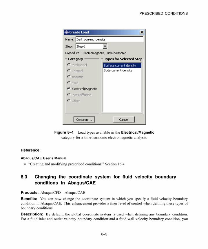
PRESCRIBED CONDITIONS
Figure 8–1 Load types available in the Electrical/Magneticcategory for a time-harmonic electromagnetic analysis.
Reference:
Abaqus/CAE User’s Manual
• “Creating and modifying prescribed conditions,” Section 16.4
8.3 Changing the coordinate system for fluid velocity boundaryconditions in Abaqus/CAE
Products: Abaqus/CFD Abaqus/CAE
Benefits: You can now change the coordinate system in which you specify a fluid velocity boundary
condition in Abaqus/CAE. This enhancement provides a finer level of control when defining these types of
boundary conditions.
Description: By default, the global coordinate system is used when defining any boundary condition.
For a fluid inlet and outlet velocity boundary condition and a fluid wall velocity boundary condition, you
8–3
Abaqus ID:
Printed on:
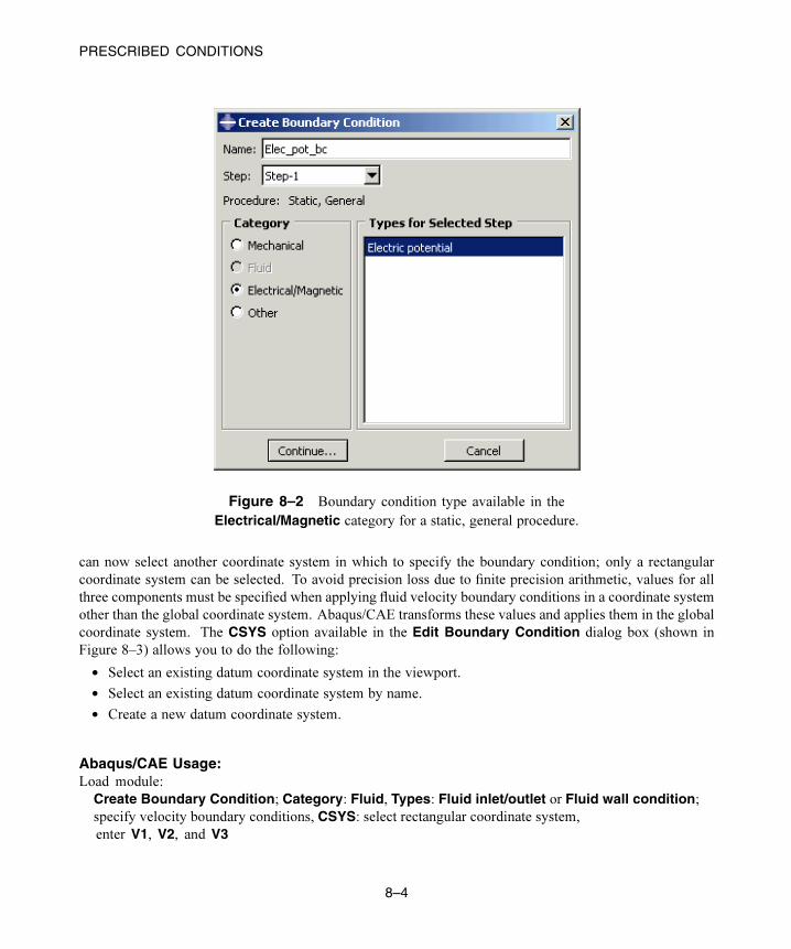
PRESCRIBED CONDITIONS
Figure 8–2 Boundary condition type available in the
Electrical/Magnetic category for a static, general procedure.
can now select another coordinate system in which to specify the boundary condition; only a rectangular
coordinate system can be selected. To avoid precision loss due to finite precision arithmetic, values for all
three components must be specified when applying fluid velocity boundary conditions in a coordinate system
other than the global coordinate system. Abaqus/CAE transforms these values and applies them in the global
coordinate system. The CSYS option available in the Edit Boundary Condition dialog box (shown in
Figure 8–3) allows you to do the following:
• Select an existing datum coordinate system in the viewport.
• Select an existing datum coordinate system by name.
• Create a new datum coordinate system.
Abaqus/CAE Usage:Load module:
Create Boundary Condition; Category: Fluid, Types: Fluid inlet/outlet or Fluid wall condition;specify velocity boundary conditions, CSYS: select rectangular coordinate system,
enter V1, V2, and V3
8–4
Abaqus ID:
Printed on:
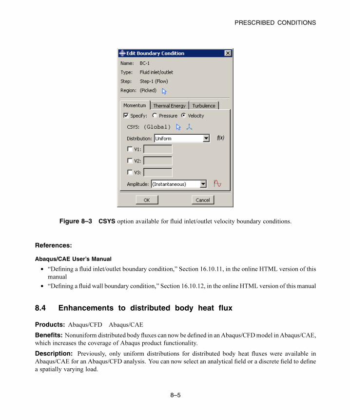
PRESCRIBED CONDITIONS
Figure 8–3 CSYS option available for fluid inlet/outlet velocity boundary conditions.
References:
Abaqus/CAE User’s Manual
• “Defining a fluid inlet/outlet boundary condition,” Section 16.10.11, in the online HTML version of this
manual
• “Defining a fluid wall boundary condition,” Section 16.10.12, in the online HTML version of this manual
8.4 Enhancements to distributed body heat flux
Products: Abaqus/CFD Abaqus/CAE
Benefits: Nonuniform distributed body fluxes can now be defined in anAbaqus/CFDmodel in Abaqus/CAE,
which increases the coverage of Abaqus product functionality.
Description: Previously, only uniform distributions for distributed body heat fluxes were available in
Abaqus/CAE for an Abaqus/CFD analysis. You can now select an analytical field or a discrete field to define
a spatially varying load.
8–5
Abaqus ID:
Printed on:
PRESCRIBED CONDITIONS
Abaqus/CAE Usage:All modules:
Model→Create; Model type: CFDLoad module:
Create Load; Category: Thermal, Type: Body heat flux; Distribution: select analytical fieldor discrete field
Reference:
Abaqus/CAE User’s Manual
• “Defining a body heat flux,” Section 16.9.18, in the online HTML version of this manual
8.5 Impedance conditions in modal steady-state dynamic analysis
Product: Abaqus/Standard
Benefits: You can now perform subspace-based steady-state dynamic acoustic analysis with impedance
conditions based on eigenmodes extracted by the AMS eigensolver.
Description: You can define impedance conditions in subspace-based steady-state dynamic analysis if the
proceeding eigenvalue extraction step is performed using the AMS eigensolver or the Lanczos eigensolver
based on the SIM architecture. Both acoustic and coupled structural-acoustic analyses are supported. You
should expect reduced analysis time because the SIM architecture is much more efficient than the traditional
architecture for large-scale linear dynamic analyses.
References:
Abaqus Analysis User’s Manual
• “Acoustic, shock, and coupled acoustic-structural analysis,” Section 6.10.1
• “Dynamic analysis procedures: overview,” Section 6.3.1
8.6 Fluid cavity pressure predefined fields and boundary conditionsin Abaqus/CAE
Products: Abaqus/Standard Abaqus/Explicit Abaqus/CAE
Benefits: You can now create fluid cavity pressure fields and boundary conditions in Abaqus/CAE. Fluid
cavity pressure predefined fields and boundary conditions are used in conjunction with fluid cavity interactions
(for more information, see “Surface fluid cavities and fluid exchanges in Abaqus/CAE,” Section 10.1). The
cavity pressure is used to specify the behavior of the cavity within an analysis and to specify flow rates in
fluid exchange interactions.
8–6
Abaqus ID:
Printed on:
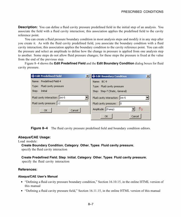
PRESCRIBED CONDITIONS
Description: You can define a fluid cavity pressure predefined field in the initial step of an analysis. You
associate the field with a fluid cavity interaction; this association applies the predefined field to the cavity
reference point.
You can create a fluid pressure boundary condition in most analysis steps and modify it in any step after
you create it. As with the fluid cavity predefined field, you associate the boundary condition with a fluid
cavity interaction; this association applies the boundary condition to the cavity reference point. You can edit
the pressure and select an amplitude to define how the change in pressure is applied from one analysis step
to another. Some steps do not allow fluid pressure changes; for these steps the pressure is fixed at the value
from the end of the previous step.
Figure 8–4 shows the Edit Predefined Field and the Edit Boundary Condition dialog boxes for fluid
cavity pressure.
Figure 8–4 The fluid cavity pressure predefined field and boundary condition editors.
Abaqus/CAE Usage:Load module:
Create Boundary Condition; Category: Other, Types: Fluid cavity pressure;specify the fluid cavity interaction
Create Predefined Field; Step: Initial, Category: Other, Types: Fluid cavity pressure;specify the fluid cavity interaction
References:
Abaqus/CAE User’s Manual
• “Defining a fluid cavity pressure boundary condition,” Section 16.10.15, in the online HTML version of
this manual
• “Defining a fluid cavity pressure field,” Section 16.11.15, in the online HTML version of this manual
8–7
Abaqus ID:
Printed on:
PRESCRIBED CONDITIONS
8.7 New rotordynamic load
Product: Abaqus/Standard
Benefits: A new distributed rotordynamic load (ROTDYNF) is available that can be used to study complex
dynamic behaviors (induced by gyroscopic moments) such as critical speeds, unbalanced responses, and
whirling phenomena in rotating structures.
Description: The rotordynamic load (ROTDYNF) is a special load type that can be used to study the
vibrational response of three-dimensional models of axisymmetric structures, such as a flywheel in a hybrid
energy storage system, that are spinning about their axes of symmetry in a fixed reference frame. This is in
contrast to the previously available centrifugal loads, Coriolis forces, and rotary acceleration loads, which are
formulated in a rotating frame. The intended workflow for the rotordynamic load is to define it in a nonlinear
static step to establish the centrifugal load effects and load stiffness terms associated with a spinning body.
The nonlinear static step can then be followed by a sequence of linear dynamic analyses (such as complex
eigenvalue extraction and/or a subspace or direct solution steady-state dynamic analysis) to study complex
dynamic behaviors.
References:
Abaqus Analysis User’s Manual
• “Distributed loads,” Section 33.4.3
Abaqus Keywords Reference Manual
• *DLOAD
8.8 New porous drag body force load in Abaqus/CFD
Products: Abaqus/CFD Abaqus/CAE
Benefits: A new distributed porous drag force load (PDBF) is available that can be used to study flows
through porous media.
Description: The porous drag body force load is used to study the flow through porous media. The value
of porosity is specified as the load.
Abaqus/CAE Usage:Load module:
Create Load; Category: Fluid, Types: Porous drag body force
References:
Abaqus Analysis User’s Manual
• “Porous media flows” in “Incompressible fluid dynamic analysis,” Section 6.6.2
8–8
Abaqus ID:
Printed on:
PRESCRIBED CONDITIONS
• “Permeability,” Section 26.6.2
• “Fluid element library,” Section 28.2.2
Abaqus/CAE User’s Manual
• “Defining a porous drag body force,” Section 16.9.24, in the online HTML version of this manual
Abaqus Keywords Reference Manual
• *DLOAD
• *FLUID SECTION
• *PERMEABILITY
8.9 New passive outflow boundary type in Abaqus/CFD
Product: Abaqus/CFD
Benefits: A new boundary condition for passive outflow can now be defined in an Abaqus/CFD analysis.
Description: The passive outflow boundary condition can be used to improve the analysis stability when
reverse flow occurs at the outlet.
References:
Abaqus Analysis User’s Manual
• “Boundary conditions in Abaqus/CFD,” Section 33.3.2
Abaqus Keywords Reference Manual
• *FLUID BOUNDARY
8.10 Pressure boundary condition that varies with the total volumeof fluid crossing a surface in Abaqus/CFD
Product: Abaqus/CFD
Benefits: A new boundary condition for fluid pressure that varies with the total volume of fluid crossing a
surface can now be defined in an Abaqus/CFD analysis.
Description: This capability can be used to define pressure boundary conditions that vary with the total
volume of fluid crossing a surface in an Abaqus/CFD analysis.
8–9
Abaqus ID:
Printed on:
PRESCRIBED CONDITIONS
References:
Abaqus Analysis User’s Manual
• “Boundary conditions in Abaqus/CFD,” Section 33.3.2
Abaqus Keywords Reference Manual
• *FLUID BOUNDARY
8.11 Base motion boundary conditions and PSD amplitudes inAbaqus/CAE
Products: Abaqus/Standard Abaqus/CAE
Benefits: New base motion boundary conditions and PSD amplitudes are available in Abaqus/CAE, which
increases the coverage of Abaqus product functionality.
Description: In Abaqus/CAE you can now define base motion boundary conditions for modal superposition
analyses. Two types of boundary conditions are available: base motion and secondary base.
You can create a boundary condition to specify the base motion of nodes in a modal dynamic step,
steady-state dynamic (mode-based or subspace-based) step, or random response step. The base motion can
be acceleration, velocity, or displacement. You can create a secondary base motion boundary condition in a
frequency extraction step.
The new PSD definition amplitude type allows you to define a frequency function that defines the
frequency dependence of the random loading in a random response analysis step. This amplitude curve
represents the power spectral density function for the random noise source. The PSD amplitude can be
referenced in the correlation definition of a base motion boundary condition in a random response step.
Abaqus/CAE Usage:Load module:
Create Boundary Condition; Step: step; Category: Mechanical; Types for Selected Step:Displacement base motion or Velocity base motion or Acceleration base motionCreate Boundary Condition; Step: step; Category: Mechanical; Types for Selected Step:Secondary base
Step module, Interaction module, or Load module:
Tools→Amplitude→Create; Type: PSD Definition
References:
Abaqus Analysis User’s Manual
• “Natural frequency extraction,” Section 6.3.5
• “Transient modal dynamic analysis,” Section 6.3.7
8–10
Abaqus ID:
Printed on:
PRESCRIBED CONDITIONS
• “Mode-based steady-state dynamic analysis,” Section 6.3.8
• “Subspace-based steady-state dynamic analysis,” Section 6.3.9
• “Random response analysis,” Section 6.3.11
• “Prescribing boundary conditions in linear perturbation steps” in “Boundary conditions in
Abaqus/Standard and Abaqus/Explicit,” Section 33.3.1
Abaqus/CAE User’s Manual
• “Defining a base motion boundary condition,” Section 16.10.8, in the online HTML version of this
manual
• “Defining a secondary base motion boundary condition,” Section 16.10.9, in the online HTML version
of this manual
• “Defining a PSD definition,” Section 57.13, in the online HTML version of this manual
8.12 Total flux distribution option for surface heat flux in Abaqus/CAE
Product: Abaqus/CAE
Benefits: When defining surface heat flux, you can choose the new total flux option for the load distribution.
This allows you to simply enter the total magnitude of flux applied over the surface. In previous releases, using
the uniform distribution option, it was necessary to query the faces of the surface to find the total area and
then divide the total flux by the surface area. With the new total flux option, you can simply enter the total
magnitude of flux applied over the entire surface.
Description: When modeling surface heat flux, you usually know the total flux that will be applied to a face
or surface of the model. In previous releases of Abaqus/CAE, this number had to be divided by the surface
area before entering it into the Magnitude field of the Edit Load dialog box (using the existing Uniformoption for Distribution). Now, with the Total Flux option (shown in Figure 8–5), you can directly enter the
total magnitude of the flux.
Abaqus/CAE Usage:Load module:
Create Load; Category: Thermal, Types: Surface heat flux; select surfaces;Distribution: Total Flux
Reference:
Abaqus/CAE User’s Manual
• “Defining a surface heat flux,” Section 16.9.17, in the online HTML version of this manual
8–11
Abaqus ID:
Printed on:
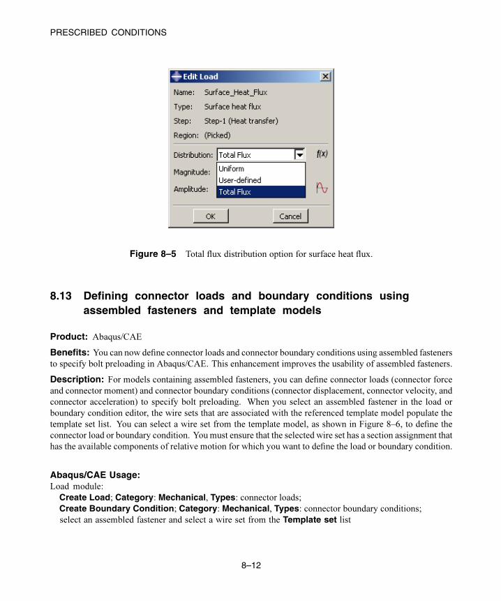
PRESCRIBED CONDITIONS
Figure 8–5 Total flux distribution option for surface heat flux.
8.13 Defining connector loads and boundary conditions usingassembled fasteners and template models
Product: Abaqus/CAE
Benefits: You can now define connector loads and connector boundary conditions using assembled fasteners
to specify bolt preloading in Abaqus/CAE. This enhancement improves the usability of assembled fasteners.
Description: For models containing assembled fasteners, you can define connector loads (connector force
and connector moment) and connector boundary conditions (connector displacement, connector velocity, and
connector acceleration) to specify bolt preloading. When you select an assembled fastener in the load or
boundary condition editor, the wire sets that are associated with the referenced template model populate the
template set list. You can select a wire set from the template model, as shown in Figure 8–6, to define the
connector load or boundary condition. You must ensure that the selected wire set has a section assignment that
has the available components of relative motion for which you want to define the load or boundary condition.
Abaqus/CAE Usage:Load module:
Create Load; Category: Mechanical, Types: connector loads;Create Boundary Condition; Category: Mechanical, Types: connector boundary conditions;
select an assembled fastener and select a wire set from the Template set list
8–12
Abaqus ID:
Printed on:

PRESCRIBED CONDITIONS
Figure 8–6 Selecting a wire set from a template model to define a connector force.
References:
Abaqus/CAE User’s Manual
• “Creating loads,” Section 16.8.1, in the online HTML version of this manual
• “Creating boundary conditions,” Section 16.8.2, in the online HTML version of this manual
8–13
Abaqus ID:
Printed on:

CONSTRAINTS
9. Constraints
This chapter discusses kinematic constraints. It provides an overview of the following enhancements:
• “Enhancements to tie constraint deletion due to element erosion,” Section 9.1
• “Improved performance for connector elements,” Section 9.2
9.1 Enhancements to tie constraint deletion due to element erosion
Product: Abaqus/Explicit
Benefits: An enhancement to nullify tie constraints when the underlying master elements are deleted
improves the robustness of the analysis.
Description: In Abaqus/Explicit tie constraints are nullified as underlying elements of tied surfaces are
deleted due to material point failure. The tie constraint between a slave node and its corresponding master
nodes is deleted when either all the elements attached to the slave node are deleted or the master element to
which the slave node is tied is deleted.
References:
Abaqus Analysis User’s Manual
• “Mesh tie constraints,” Section 34.3.1
Abaqus Keywords Reference Manual
• *TIE
9.2 Improved performance for connector elements
Product: Abaqus/Explicit
Benefits: Improved performance is achieved for connector elements without kinematic constraints or
constitutive behavior.
Description: In Abaqus/Explicit connector elements without kinematic constraints or constitutive behavior
are now solved without invoking the implicit solver. This change improves the performance of the analysis
particularly when such connectors overlap with other constraints, such as slave nodes of tie constraints.
References:
Abaqus Analysis User’s Manual
• “Connector elements,” Section 31.1.2
9–1
Abaqus ID:
Printed on:

CONSTRAINTS
Abaqus Keywords Reference Manual
• *CONNECTOR SECTION
9–2
Abaqus ID:
Printed on:
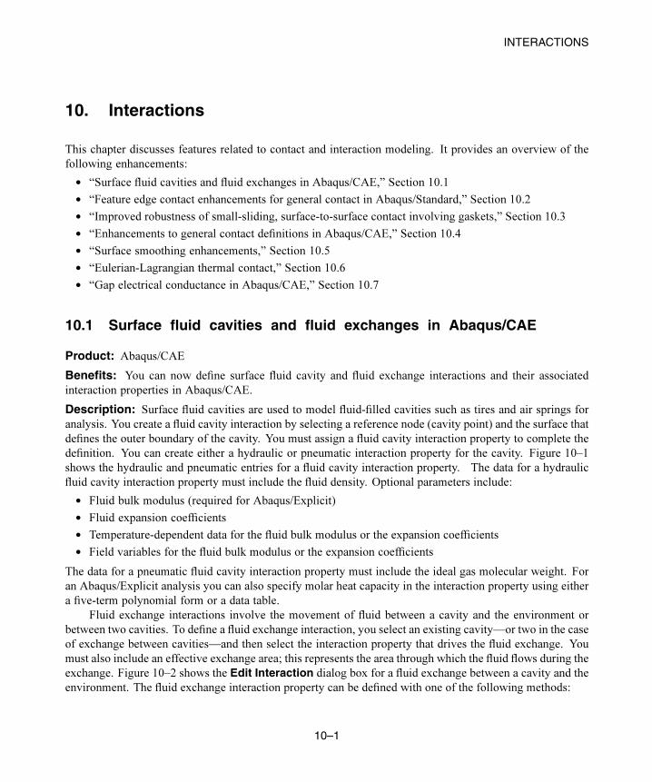
INTERACTIONS
10. Interactions
This chapter discusses features related to contact and interaction modeling. It provides an overview of the
following enhancements:
• “Surface fluid cavities and fluid exchanges in Abaqus/CAE,” Section 10.1
• “Feature edge contact enhancements for general contact in Abaqus/Standard,” Section 10.2
• “Improved robustness of small-sliding, surface-to-surface contact involving gaskets,” Section 10.3
• “Enhancements to general contact definitions in Abaqus/CAE,” Section 10.4
• “Surface smoothing enhancements,” Section 10.5
• “Eulerian-Lagrangian thermal contact,” Section 10.6
• “Gap electrical conductance in Abaqus/CAE,” Section 10.7
10.1 Surface fluid cavities and fluid exchanges in Abaqus/CAE
Product: Abaqus/CAE
Benefits: You can now define surface fluid cavity and fluid exchange interactions and their associated
interaction properties in Abaqus/CAE.
Description: Surface fluid cavities are used to model fluid-filled cavities such as tires and air springs for
analysis. You create a fluid cavity interaction by selecting a reference node (cavity point) and the surface that
defines the outer boundary of the cavity. You must assign a fluid cavity interaction property to complete the
definition. You can create either a hydraulic or pneumatic interaction property for the cavity. Figure 10–1
shows the hydraulic and pneumatic entries for a fluid cavity interaction property. The data for a hydraulic
fluid cavity interaction property must include the fluid density. Optional parameters include:
• Fluid bulk modulus (required for Abaqus/Explicit)
• Fluid expansion coefficients
• Temperature-dependent data for the fluid bulk modulus or the expansion coefficients
• Field variables for the fluid bulk modulus or the expansion coefficients
The data for a pneumatic fluid cavity interaction property must include the ideal gas molecular weight. For
an Abaqus/Explicit analysis you can also specify molar heat capacity in the interaction property using either
a five-term polynomial form or a data table.
Fluid exchange interactions involve the movement of fluid between a cavity and the environment or
between two cavities. To define a fluid exchange interaction, you select an existing cavity—or two in the case
of exchange between cavities—and then select the interaction property that drives the fluid exchange. You
must also include an effective exchange area; this represents the area through which the fluid flows during the
exchange. Figure 10–2 shows the Edit Interaction dialog box for a fluid exchange between a cavity and the
environment. The fluid exchange interaction property can be defined with one of the following methods:
10–1
Abaqus ID:
Printed on:
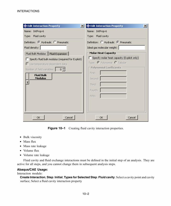
INTERACTIONS
Figure 10–1 Creating fluid cavity interaction properties.
• Bulk viscosity
• Mass flux
• Mass rate leakage
• Volume flux
• Volume rate leakage
Fluid cavity and fluid exchange interactions must be defined in the initial step of an analysis. They are
active for all steps, and you cannot change them in subsequent analysis steps.
Abaqus/CAE Usage:Interaction module:
Create Interaction;Step: Initial;Types for Selected Step:Fluid cavity: Select a cavity point and cavitysurface; Select a fluid cavity interaction property
10–2
Abaqus ID:
Printed on:
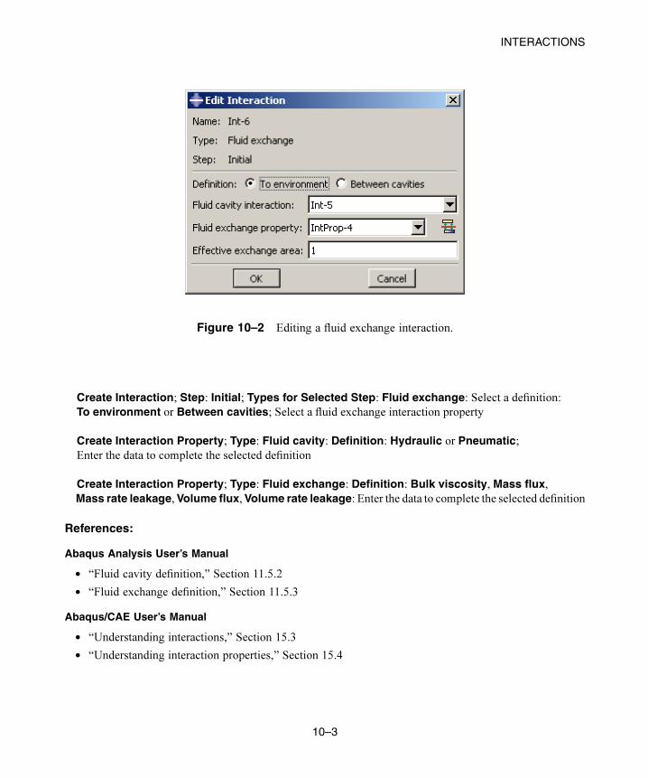
INTERACTIONS
Figure 10–2 Editing a fluid exchange interaction.
Create Interaction; Step: Initial; Types for Selected Step: Fluid exchange: Select a definition:To environment or Between cavities; Select a fluid exchange interaction property
Create Interaction Property; Type: Fluid cavity: Definition: Hydraulic or Pneumatic;Enter the data to complete the selected definition
Create Interaction Property; Type: Fluid exchange: Definition: Bulk viscosity, Mass flux,Mass rate leakage,Volume flux,Volume rate leakage: Enter the data to complete the selected definition
References:
Abaqus Analysis User’s Manual
• “Fluid cavity definition,” Section 11.5.2
• “Fluid exchange definition,” Section 11.5.3
Abaqus/CAE User’s Manual
• “Understanding interactions,” Section 15.3
• “Understanding interaction properties,” Section 15.4
10–3
Abaqus ID:
Printed on:
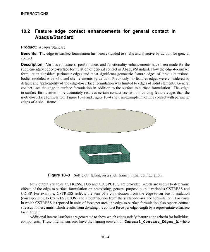
INTERACTIONS
10.2 Feature edge contact enhancements for general contact inAbaqus/Standard
Product: Abaqus/Standard
Benefits: The edge-to-surface formulation has been extended to shells and is active by default for general
contact
Description: Various robustness, performance, and functionality enhancements have been made for the
supplementary edge-to-surface formulation of general contact in Abaqus/Standard. Now the edge-to-surface
formulation considers perimeter edges and most significant geometric feature edges of three-dimensional
bodies modeled with solid and shell elements by default. Previously, no features edges were considered by
default and applicability of the edge-to-surface formulation was limited to edges of solid elements. General
contact uses the edge-to-surface formulation in addition to the surface-to-surface formulation. The edge-
to-surface formulation more accurately resolves certain contact scenarios involving feature edges than the
node-to-surface formulation. Figure 10–3 and Figure 10–4 show an example involving contact with perimeter
edges of a shell frame.
Figure 10–3 Soft cloth falling on a shell frame: initial configuration.
New output variables CSTRESSETOS and CDISPETOS are provided, which are useful to determine
effects of the edge-to-surface formulation on preexisting, general-purpose output variables CSTRESS and
CDISP. For example, CSTRESS reflects the sum of a contribution from the edge-to-surface formulation
(corresponding to CSTRESSETOS) and a contribution from the surface-to-surface formulation. For cases
in which CSTRESS is reported in units of force per area, the edge-to-surface formulation also reports contact
stresses in these units, which results from dividing the contact force per edge length by a representative surface
facet length.
Additional internal surfaces are generated to showwhich edges satisfy feature edge criteria for individual
components. These internal surfaces have the naming convention General_Contact_Edges_k, where
10–4
Abaqus ID:
Printed on:
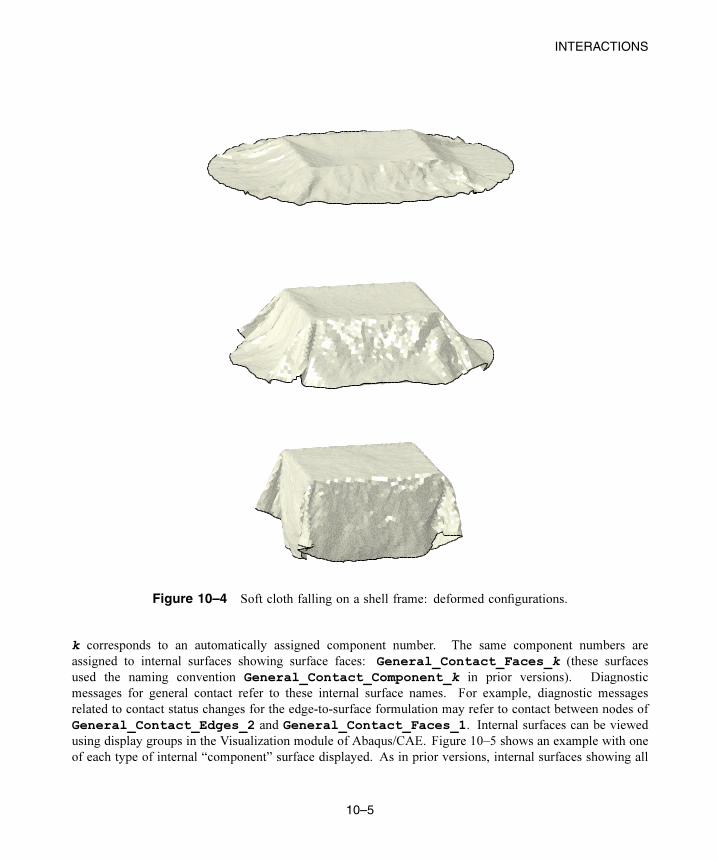
INTERACTIONS
Figure 10–4 Soft cloth falling on a shell frame: deformed configurations.
k corresponds to an automatically assigned component number. The same component numbers are
assigned to internal surfaces showing surface faces: General_Contact_Faces_k (these surfaces
used the naming convention General_Contact_Component_k in prior versions). Diagnostic
messages for general contact refer to these internal surface names. For example, diagnostic messages
related to contact status changes for the edge-to-surface formulation may refer to contact between nodes of
General_Contact_Edges_2 and General_Contact_Faces_1. Internal surfaces can be viewed
using display groups in the Visualization module of Abaqus/CAE. Figure 10–5 shows an example with one
of each type of internal “component” surface displayed. As in prior versions, internal surfaces showing all
10–5
Abaqus ID:
Printed on:
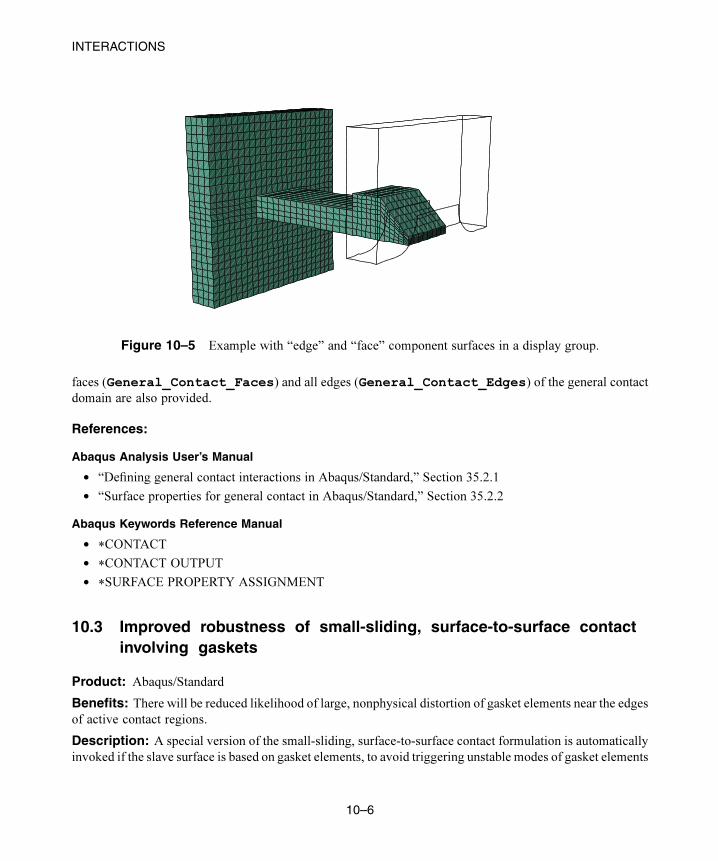
INTERACTIONS
Figure 10–5 Example with “edge” and “face” component surfaces in a display group.
faces (General_Contact_Faces) and all edges (General_Contact_Edges) of the general contact
domain are also provided.
References:
Abaqus Analysis User’s Manual
• “Defining general contact interactions in Abaqus/Standard,” Section 35.2.1
• “Surface properties for general contact in Abaqus/Standard,” Section 35.2.2
Abaqus Keywords Reference Manual
• *CONTACT
• *CONTACT OUTPUT
• *SURFACE PROPERTY ASSIGNMENT
10.3 Improved robustness of small-sliding, surface-to-surface contactinvolving gaskets
Product: Abaqus/Standard
Benefits: There will be reduced likelihood of large, nonphysical distortion of gasket elements near the edges
of active contact regions.
Description: A special version of the small-sliding, surface-to-surface contact formulation is automatically
invoked if the slave surface is based on gasket elements, to avoid triggering unstable modes of gasket elements
10–6
Abaqus ID:
Printed on:
INTERACTIONS
in certain situations. Gasket elements have very little resistance to certain shear deformation modes, which are
not significant in common gasket applications; however, having multiple slave nodes per contact constraint,
such as with regular surface-to-surface discretization, can trigger these modes at boundaries of an active
contact region and regions with a large contact-pressure gradient. Now, the small-sliding, surface-to-surface
contact formulation uses a single slave node per contact constraint if the slave surface is based on gasket
elements (like the node-to-surface contact formulations), but it remains capable of providing accurate contact
stress predictions despite having mismatched meshes across the contact interface.
The finite-sliding, surface-to-surface formulation always uses multiple slave nodes per contact constraint
and is not recommended for contact involving gasket elements.
References:
Abaqus Analysis User’s Manual
• “Using the small-sliding tracking approach” in “Contact formulations in Abaqus/Standard,”
Section 37.1.1
Abaqus Keywords Reference Manual
• *CONTACT PAIR
10.4 Enhancements to general contact definitions in Abaqus/CAE
Products: Abaqus/Standard Abaqus/Explicit Abaqus/CAE
Benefits: Several advanced options for general contact definitions can now be specified in Abaqus/CAE.
These enhancements augment the capabilities for creating complex general contact interactions within
Abaqus/CAE.
Description: The following options associated with a general contact interaction can now be defined in
Abaqus/CAE:
• Contact stabilization in an Abaqus/Standard interaction
• Specification of “feature edges” in an Abaqus/Standard interaction
• Additional methods for defining feature edges in an Abaqus/Explicit interaction
• Specification of an interference distance as part of a contact initialization in Abaqus/Standard
• Specification of an initial clearance distance as part of a contact initialization in Abaqus/Standard
Contact stabilization introduces viscous damping to oppose incremental relative motion between two
surfaces in an Abaqus/Standard general contact interaction. The main purpose of the damping is to stabilize
rigid bodymotion before the surfaces come into contact, at which point contact and frictional forces counteract
the motion. A contact stabilization definition is created in Abaqus/CAE using the contact stabilization editor;
you provide a name for the stabilization definition and a set of stabilization factors (see Figure 10–6).
10–7
Abaqus ID:
Printed on:
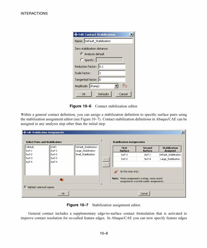
INTERACTIONS
Figure 10–6 Contact stabilization editor.
Within a general contact definition, you can assign a stabilization definition to specific surface pairs using
the stabilization assignment editor (see Figure 10–7). Contact stabilization definitions in Abaqus/CAE can be
assigned in any analysis step other than the initial step.
Figure 10–7 Stabilization assignment editor.
General contact includes a supplementary edge-to-surface contact formulation that is activated to
improve contact resolution for so-called feature edges. In Abaqus/CAE you can now specify feature edges
10–8
Abaqus ID:
Printed on:
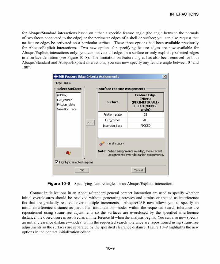
INTERACTIONS
for Abaqus/Standard interactions based on either a specific feature angle (the angle between the normals
of two facets connected to the edge) or the perimeter edges of a shell or surface; you can also request that
no feature edges be activated on a particular surface. These three options had been available previously
for Abaqus/Explicit interactions. Two new options for specifying feature edges are now available for
Abaqus/Explicit interactions only: you can activate all edges in a surface or only explicitly selected edges
in a surface definition (see Figure 10–8). The limitation on feature angles has also been removed for both
Abaqus/Standard and Abaqus/Explicit interactions; you can now specify any feature angle between 0° and
180°.
Figure 10–8 Specifying feature angles in an Abaqus/Explicit interaction.
Contact initializations in an Abaqus/Standard general contact interaction are used to specify whether
initial overclosures should be resolved without generating stresses and strains or treated as interference
fits that are gradually resolved over multiple increments. Abaqus/CAE now allows you to specify an
initial interference distance as part of an initialization—nodes within the requested search tolerance are
repositioned using strain-free adjustments so the surfaces are overclosed by the specified interference
distance; the overclosure is resolved as an interference fit when the analysis begins. You can also now specify
an initial clearance distance—nodes within the requested search tolerance are repositioned using strain-free
adjustments so the surfaces are separated by the specified clearance distance. Figure 10–9 highlights the new
options in the contact initialization editor.
10–9
Abaqus ID:
Printed on:
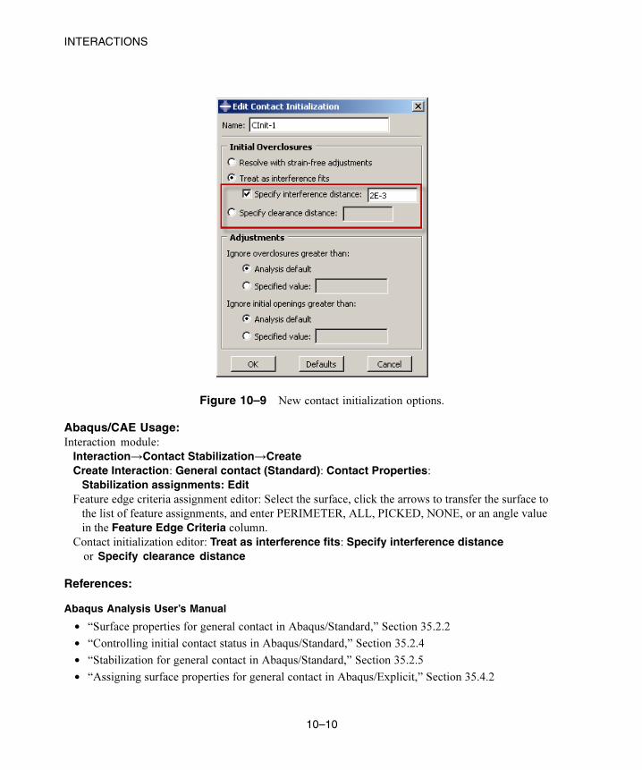
INTERACTIONS
Figure 10–9 New contact initialization options.
Abaqus/CAE Usage:Interaction module:
Interaction→Contact Stabilization→CreateCreate Interaction: General contact (Standard): Contact Properties:
Stabilization assignments: EditFeature edge criteria assignment editor: Select the surface, click the arrows to transfer the surface to
the list of feature assignments, and enter PERIMETER, ALL, PICKED, NONE, or an angle value
in the Feature Edge Criteria column.
Contact initialization editor: Treat as interference fits: Specify interference distanceor Specify clearance distance
References:
Abaqus Analysis User’s Manual
• “Surface properties for general contact in Abaqus/Standard,” Section 35.2.2
• “Controlling initial contact status in Abaqus/Standard,” Section 35.2.4
• “Stabilization for general contact in Abaqus/Standard,” Section 35.2.5
• “Assigning surface properties for general contact in Abaqus/Explicit,” Section 35.4.2
10–10
Abaqus ID:
Printed on:
INTERACTIONS
Abaqus/CAE User’s Manual
• “Creating contact initializations,” Section 15.12.4, in the online HTML version of this manual
• “Creating contact stabilization definitions,” Section 15.12.5, in the online HTML version of this manual
• “Specifying and modifying contact initialization assignments for general contact,” Section 15.13.3, in
the online HTML version of this manual
• “Specifying and modifying contact stabilization assignments for general contact,” Section 15.13.4, in
the online HTML version of this manual
• “Specifying surface property assignments for general contact,” Section 15.13.5, in the online HTML
version of this manual
10.5 Surface smoothing enhancements
Products: Abaqus/Standard Abaqus/Explicit Abaqus/CAE
Benefits: Surface smoothing methods improve the accuracy of contact stresses and reduce solution noise
for common types of curved contact surfaces.
Description: Faceted representations of curved surfaces often lead to inaccuracies in contact stresses and
other types of solution noise. Circumferential and spherical smoothing methods have been available in
previous releases of Abaqus/Standard to enhance robustness and solution accuracy for surface-to-surface
contact formulations involving element-based surfaces. These smoothing methods introduce geometric
corrections to better represent the curved shape, and they remain effective after relative motion between
contact surfaces. The circumferential and spherical smoothing methods are now also available in
Abaqus/Explicit for general contact. Furthermore, a toroidal smoothing method has been added for
Abaqus/Standard and Abaqus/Explicit; the toroidal smoothing method cannot be defined in Abaqus/CAE.
For example, in the model of the ball bearing shown in Figure 10–10, spherical smoothing can be defined
on the surfaces of the balls and the retainer, and toroidal smoothing can be defined on the surfaces of the inner
and outer races that contact the balls.
Abaqus/CAE Usage:Interaction module:
General contact interaction editor:
Surface Properties: Surface smoothing assignments: Edit:Select the surface, click the arrows to transfer the surface to the list of smoothing assignments.
In the Smoothing Option column, select REVOLUTION to apply circumferential smoothing, select
SPHERICAL to apply spherical smoothing, or select NONE to prevent smoothing of the surface.
References:
Abaqus Analysis User’s Manual
• “Defining general contact interactions in Abaqus/Explicit,” Section 35.4.1
10–11
Abaqus ID:
Printed on:
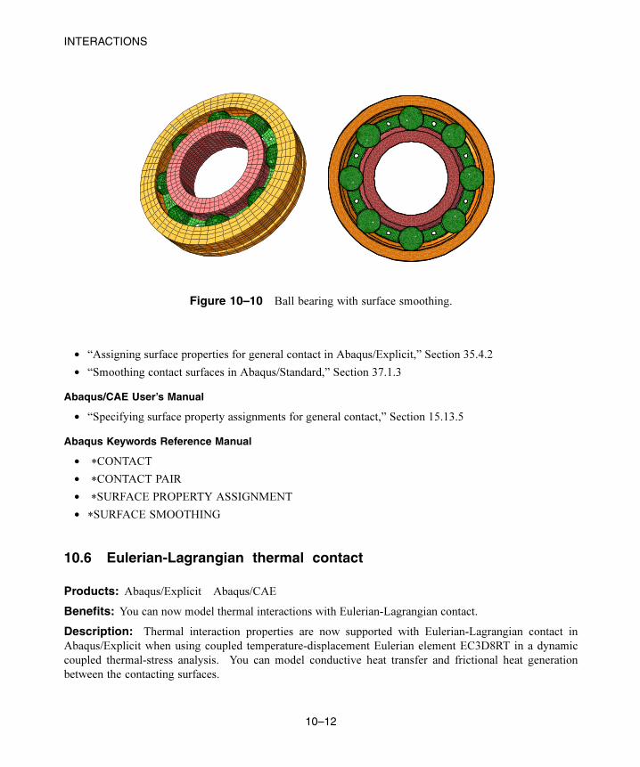
INTERACTIONS
Figure 10–10 Ball bearing with surface smoothing.
• “Assigning surface properties for general contact in Abaqus/Explicit,” Section 35.4.2
• “Smoothing contact surfaces in Abaqus/Standard,” Section 37.1.3
Abaqus/CAE User’s Manual
• “Specifying surface property assignments for general contact,” Section 15.13.5
Abaqus Keywords Reference Manual
• *CONTACT
• *CONTACT PAIR
• *SURFACE PROPERTY ASSIGNMENT
• *SURFACE SMOOTHING
10.6 Eulerian-Lagrangian thermal contact
Products: Abaqus/Explicit Abaqus/CAE
Benefits: You can now model thermal interactions with Eulerian-Lagrangian contact.
Description: Thermal interaction properties are now supported with Eulerian-Lagrangian contact in
Abaqus/Explicit when using coupled temperature-displacement Eulerian element EC3D8RT in a dynamic
coupled thermal-stress analysis. You can model conductive heat transfer and frictional heat generation
between the contacting surfaces.
10–12
Abaqus ID:
Printed on:
INTERACTIONS
References:
Abaqus Analysis User’s Manual
• “Eulerian analysis,” Section 14.1.1
• “Thermal contact properties,” Section 36.2.1
Abaqus/CAE User’s Manual
• “Defining a contact interaction property,” Section 15.14.1
• “Defining contact in Eulerian-Lagrangian models,” Section 28.3
Abaqus Keywords Reference Manual
• *CONTACT
• *GAP CONDUCTANCE
• *GAP HEAT GENERATION
• *SURFACE INTERACTION
10.7 Gap electrical conductance in Abaqus/CAE
Products: Abaqus/Standard Abaqus/CAE
Benefits: You can now define gap electrical conductance as a contact interaction property in Abaqus/CAE,
which increases the coverage of Abaqus product functionality.
Description: You can use the contact property editor in Abaqus/CAE to define the electrical conductance
between two surfaces in a contact interaction. The conductance is proportional to the difference in electric
potentials across the interface. The conduction is a function of the clearance (separation) between the
surfaces and can be a function of the contact pressure. The Edit Contact Property dialog box lets you enter
conductance values in a data table, providing clearance-dependency data and/or pressure-dependency data.
Abaqus/CAE Usage:Interaction module:
Contact property editor: Electrical→Electrical Conductance
References:
Abaqus Analysis User’s Manual
• “Electrical contact properties,” Section 36.3.1
Abaqus/CAE User’s Manual
• “Specifying gap conductance for electrical contact property options” in “Defining a contact interaction
property,” Section 15.14.1, in the online HTML version of this manual
10–13
Abaqus ID:
Printed on:

ENGINEERING FEATURES
11. Engineering features
This chapter discusses engineering features related to part and assembly modeling in Abaqus/CAE. It provides
an overview of the following enhancement:
• “Defining a seam in an Abaqus/CFD analysis,” Section 11.1
11.1 Defining a seam in an Abaqus/CFD analysis
Products: Abaqus/CFD Abaqus/CAE
Benefits: The ability to define seams in an Abaqus/CFD analysis simplifies the modeling process for fluid-
structure interaction analyses involving shells/membranes.
Description: You can now define a seam in an Abaqus/CFD analysis. For an Abaqus/CFD analysis involved
in a fluid-structure interaction with shells/membranes, a seam defines a zero-thickness shell in the mesh. You
can create a double-sided surface that represents the seam and select that surface as the region for the fluid-
structure interaction boundary.
Abaqus/CAE places overlapping duplicate nodes along a seam when the mesh is generated. A seam
cannot extend along the boundaries of a part and must be embedded within a face of a two-dimensional part
or within a cell of a solid part. Because a seam modifies the mesh, you cannot create a seam on a dependent
part instance.
Abaqus/CAE Usage:Interaction module:
Special→Crack→Assign seam
References:
Abaqus/CAE User’s Manual
• “Modeling cracks and seams” in “Using the Special menu in the Interaction module,” Section 15.12.14,
in the online HTML version of this manual
• “Defining a fluid-structure co-simulation interaction,” Section 15.13.15, in the online HTML version of
this manual
11–1
Abaqus ID:
Printed on:

MESHING
12. Meshing
This chapter discusses features related to meshing your model. It provides an overview of the following
enhancements:
• “Local controls for tetrahedral meshing,” Section 12.1
• “Combining orphan and native mesh features in a model,” Section 12.2
• “Persistent display of seeds,” Section 12.3
• “Enhanced node editing functionality,” Section 12.4
• “Dragging nodes,” Section 12.5
• “Improved display for selection of mesh parts,” Section 12.6
• “Node and element numbering in flattened input files,” Section 12.7
• “Adding a boundary layer to a tetrahedral mesh,” Section 12.8
• “Mesh retention during feature additions and modifications,” Section 12.9
12.1 Local controls for tetrahedral meshing
Product: Abaqus/CAE
Benefits: You can now apply mesh controls to selected faces of solid regions that will be meshed with
tetrahedral elements.
Description: You can now use mesh controls to assign either structured or free mesh techniques to the faces
of solid regions that will be meshed using tetrahedral elements. This option gives you greater control over the
appearance and quality of the tetrahedral mesh.
Only triangular elements can be assigned to the faces of tetrahedral regions. If you assign the structured
technique, the selected faces must follow the same geometrical and topological requirements applicable for
two-dimensional structured meshing. The new controls allow you to force Abaqus/CAE to use a structured
mesh or free mesh on selected faces, overriding the technique assigned to the rest of the faces in the region.
For example, when reviewing the boundary triangular mesh created using the default controls for a
tetrahedral region—a free mesh with mapped meshing where Abaqus/CAE determines that mapped meshing
is appropriate—you may discover faces with a free mesh where you think a mapped mesh should be used.
You can now select the desired faces and assign the structured mesh technique. Likewise, if you find faces
to which Abaqus/CAE applied mapped meshing, but the resulting triangular mesh is of poor quality, you can
assign the free mesh technique to those faces.
If you prevent Abaqus/CAE from applying mapped meshing to appropriate faces of a tetrahedral mesh
(by setting mesh controls on the region), you can use the new controls to allow mapped meshing on selected
boundary faces without changing the surface mesh for the entire region.
Figure 12–1 shows the difference between the default free meshing (left) and structured meshing (right)
on the middle section of a cylindrical mounting boss.
12–1
Abaqus ID:
Printed on:
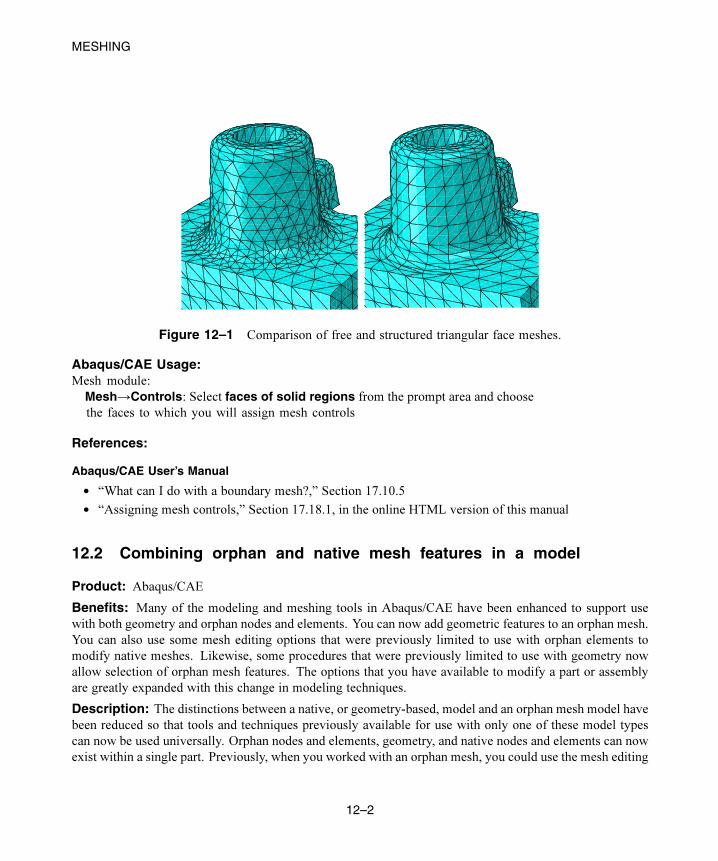
MESHING
Figure 12–1 Comparison of free and structured triangular face meshes.
Abaqus/CAE Usage:Mesh module:
Mesh→Controls: Select faces of solid regions from the prompt area and choose
the faces to which you will assign mesh controls
References:
Abaqus/CAE User’s Manual
• “What can I do with a boundary mesh?,” Section 17.10.5
• “Assigning mesh controls,” Section 17.18.1, in the online HTML version of this manual
12.2 Combining orphan and native mesh features in a model
Product: Abaqus/CAE
Benefits: Many of the modeling and meshing tools in Abaqus/CAE have been enhanced to support use
with both geometry and orphan nodes and elements. You can now add geometric features to an orphan mesh.
You can also use some mesh editing options that were previously limited to use with orphan elements to
modify native meshes. Likewise, some procedures that were previously limited to use with geometry now
allow selection of orphan mesh features. The options that you have available to modify a part or assembly
are greatly expanded with this change in modeling techniques.
Description: The distinctions between a native, or geometry-based, model and an orphan mesh model have
been reduced so that tools and techniques previously available for use with only one of these model types
can now be used universally. Orphan nodes and elements, geometry, and native nodes and elements can now
exist within a single part. Previously, when you worked with an orphan mesh, you could use the mesh editing
12–2
Abaqus ID:
Printed on:
MESHING
tools to modify the mesh, but it could be difficult to make significant changes to the model. Now you can
select an orphan element face as the sketch plane for the creation of new geometry. Likewise, some of the
tools in the Edit Mesh toolset that were previously available only for use with an orphan mesh—such as the
Offset tool—can now also be used to modify a native mesh. Other tools are available to work with the new
combined models, but you can use them only with the suitable portions of the mesh. For example, the merge
and subdivide layer mesh tools can be used in a combined model, but you can use them only on the orphan
elements.
Other enhancements related to this change include:
• Revision of the bottom-up meshing tools to extend the mesh of geometry-based parts by adding orphan
elements
• Merging part instances that include both geometry and mesh components
• Allowance for the use of datum planes and element faces in addition to geometry faces on the target side
of a bottom-up swept mesh
• Projection of nodes and element edges onto sketches
• Manual association of three-dimensional elements with geometric cells
• Association of element faces, element edges, and nodes with geometry
• Deletion of mesh-geometry association
To avoid confusion, elements are still colored according to their source; orphan elements are colored
green, and native mesh elements are colored cyan.
Note: The usages and references listed below are a sample of some of the more significant changes. Many
other procedures have been updated to incorporate selection of both geometry and orphan mesh items.
Abaqus/CAE Usage:Part module:
Shape→Solid→Extrude: Select the face of an orphan mesh element as a sketching plane
Shape→Shell→Extrude: Select the face of an orphan mesh element as a sketching plane
Mesh module:
Mesh→Edit: Category: Mesh: Associate mesh with geometry or
Delete mesh associativity
References:
Abaqus/CAE User’s Manual
• “Adding a solid feature,” Section 11.21, in the online HTML version of this manual
• “Adding a shell feature,” Section 11.22, in the online HTML version of this manual
• “Performing Boolean operations on part instances,” Section 13.6
• “Bottom-up meshing,” Section 17.11
• “Mesh-geometry association,” Section 17.12
12–3
Abaqus ID:
Printed on:
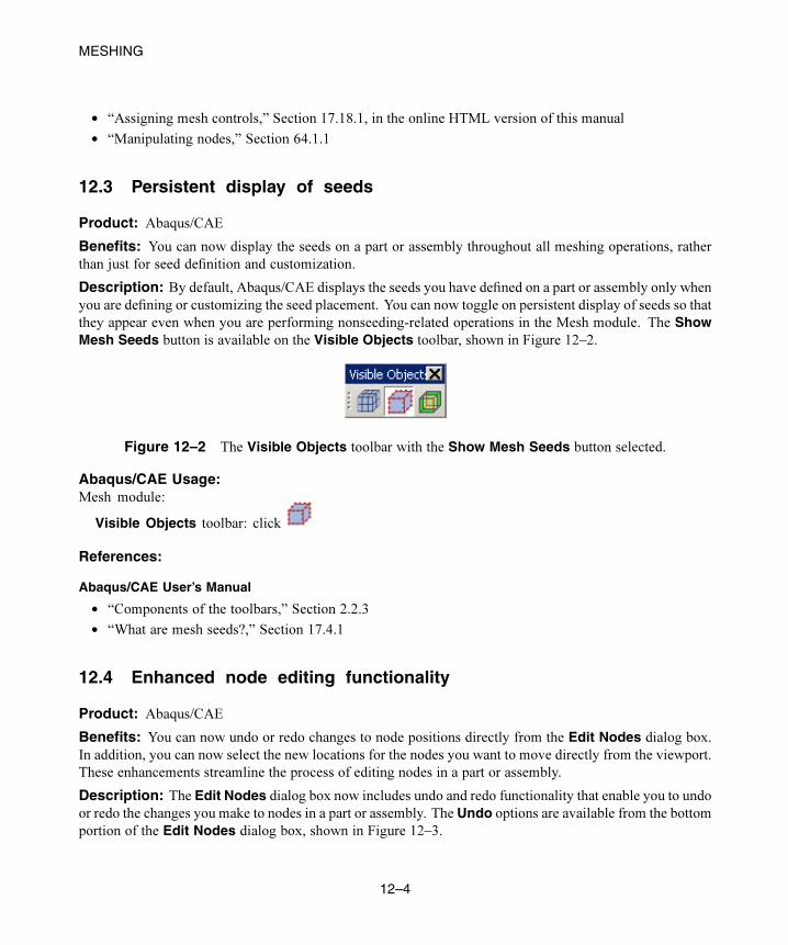
MESHING
• “Assigning mesh controls,” Section 17.18.1, in the online HTML version of this manual
• “Manipulating nodes,” Section 64.1.1
12.3 Persistent display of seeds
Product: Abaqus/CAE
Benefits: You can now display the seeds on a part or assembly throughout all meshing operations, rather
than just for seed definition and customization.
Description: By default, Abaqus/CAE displays the seeds you have defined on a part or assembly only when
you are defining or customizing the seed placement. You can now toggle on persistent display of seeds so that
they appear even when you are performing nonseeding-related operations in the Mesh module. The ShowMesh Seeds button is available on the Visible Objects toolbar, shown in Figure 12–2.
Figure 12–2 The Visible Objects toolbar with the Show Mesh Seeds button selected.
Abaqus/CAE Usage:Mesh module:
Visible Objects toolbar: click
References:
Abaqus/CAE User’s Manual
• “Components of the toolbars,” Section 2.2.3
• “What are mesh seeds?,” Section 17.4.1
12.4 Enhanced node editing functionality
Product: Abaqus/CAE
Benefits: You can now undo or redo changes to node positions directly from the Edit Nodes dialog box.
In addition, you can now select the new locations for the nodes you want to move directly from the viewport.
These enhancements streamline the process of editing nodes in a part or assembly.
Description: The Edit Nodes dialog box now includes undo and redo functionality that enable you to undo
or redo the changes you make to nodes in a part or assembly. The Undo options are available from the bottom
portion of the Edit Nodes dialog box, shown in Figure 12–3.
12–4
Abaqus ID:
Printed on:
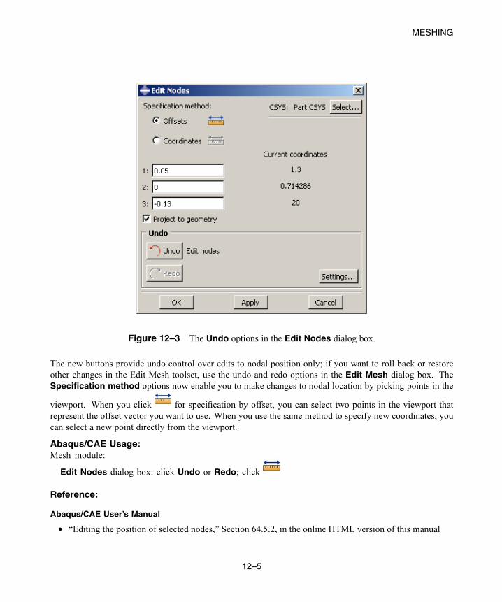
MESHING
Figure 12–3 The Undo options in the Edit Nodes dialog box.
The new buttons provide undo control over edits to nodal position only; if you want to roll back or restore
other changes in the Edit Mesh toolset, use the undo and redo options in the Edit Mesh dialog box. The
Specification method options now enable you to make changes to nodal location by picking points in the
viewport. When you click for specification by offset, you can select two points in the viewport that
represent the offset vector you want to use. When you use the same method to specify new coordinates, you
can select a new point directly from the viewport.
Abaqus/CAE Usage:Mesh module:
Edit Nodes dialog box: click Undo or Redo; click
Reference:
Abaqus/CAE User’s Manual
• “Editing the position of selected nodes,” Section 64.5.2, in the online HTML version of this manual
12–5
Abaqus ID:
Printed on:
MESHING
12.5 Dragging nodes
Product: Abaqus/CAE
Benefits: You can now modify a mesh by dragging nodes to new locations.
Description: You can drag interior and exterior nodes of a mesh to change element shape and quality. Node
dragging has been added to the node modification tools in the Edit Mesh toolset. When you activate node
dragging, Abaqus/CAE activates element quality highlighting so you can see any elements that have warnings
or failures. The highlighting is updated as you drag a node; therefore, you can immediately see whether you
are improving poor elements—or at least make certain that you are not creating more poor elements—by
moving the node.
By default, mesh nodes are constrained to the geometry with which they are associated; a dragged surface
node must stay on the original surface, an edge node must stay on the edge, and a node associated with a vertex
cannot be dragged. However, if you toggle off Project to geometry in the prompt area, you can drag nodes
to any location in a plane parallel to the screen and passing through the starting location of the node. Interior
nodes are not constrained to geometry; therefore, they are always moved in a plane parallel to the screen.
You can drag only one node at a time. You can drag orphan or native mesh nodes on dependent or
independent instances in an assembly. Dragging nodes in a dependent part instance will change the part mesh
and all instances of the part.
Abaqus/CAE Usage:Mesh module:
Edit Mesh dialog box: Category: Node: Method: Drag: toggle Project to geometry in the
prompt area: click and hold mouse button 1 to drag a node to a new location
Reference:
Abaqus/CAE User’s Manual
• “Dragging nodes,” Section 64.5.3, in the online HTML version of this manual
12.6 Improved display for selection of mesh parts
Product: Abaqus/CAE
Benefits: Abaqus/CAE now highlights only the exterior edges of a mesh part when you select the entire
mesh part in the viewport. This enhancement makes mesh part selection easier and clearer when you perform
operations that highlight the entire mesh part, such as mesh verification.
Description: When you select an entire mesh part from the viewport, Abaqus/CAE highlights only the
exterior edges of the part by default rather than the edges of all of its elements. The contrast in highlight
behavior is shown in Figure 12–4.
12–6
Abaqus ID:
Printed on:
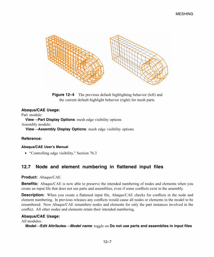
MESHING
Figure 12–4 The previous default highlighting behavior (left) and
the current default highlight behavior (right) for mesh parts.
Abaqus/CAE Usage:Part module:
View→Part Display Options: mesh edge visibility options
Assembly module:
View→Assembly Display Options: mesh edge visibility options
Reference:
Abaqus/CAE User’s Manual
• “Controlling edge visibility,” Section 76.3
12.7 Node and element numbering in flattened input files
Product: Abaqus/CAE
Benefits: Abaqus/CAE is now able to preserve the intended numbering of nodes and elements when you
create an input file that does not use parts and assemblies, even if some conflicts exist in the assembly.
Description: When you create a flattened input file, Abaqus/CAE checks for conflicts in the node and
element numbering. In previous releases any conflicts would cause all nodes or elements in the model to be
renumbered. Now Abaqus/CAE renumbers nodes and elements for only the part instances involved in the
conflict. All other nodes and elements retain their intended numbering.
Abaqus/CAE Usage:All modules:
Model→Edit Attributes→Model name: toggle on Do not use parts and assemblies in input files
12–7
Abaqus ID:
Printed on:
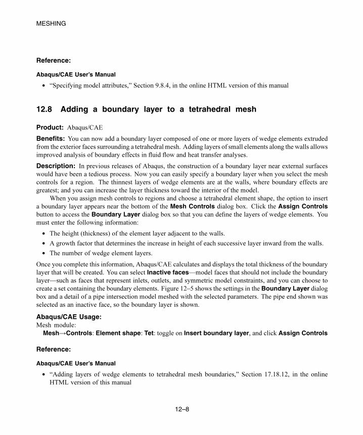
MESHING
Reference:
Abaqus/CAE User’s Manual
• “Specifying model attributes,” Section 9.8.4, in the online HTML version of this manual
12.8 Adding a boundary layer to a tetrahedral mesh
Product: Abaqus/CAE
Benefits: You can now add a boundary layer composed of one or more layers of wedge elements extruded
from the exterior faces surrounding a tetrahedral mesh. Adding layers of small elements along the walls allows
improved analysis of boundary effects in fluid flow and heat transfer analyses.
Description: In previous releases of Abaqus, the construction of a boundary layer near external surfaces
would have been a tedious process. Now you can easily specify a boundary layer when you select the mesh
controls for a region. The thinnest layers of wedge elements are at the walls, where boundary effects are
greatest; and you can increase the layer thickness toward the interior of the model.
When you assign mesh controls to regions and choose a tetrahedral element shape, the option to insert
a boundary layer appears near the bottom of the Mesh Controls dialog box. Click the Assign Controlsbutton to access the Boundary Layer dialog box so that you can define the layers of wedge elements. You
must enter the following information:
• The height (thickness) of the element layer adjacent to the walls.
• A growth factor that determines the increase in height of each successive layer inward from the walls.
• The number of wedge element layers.
Once you complete this information, Abaqus/CAE calculates and displays the total thickness of the boundary
layer that will be created. You can select Inactive faces—model faces that should not include the boundary
layer—such as faces that represent inlets, outlets, and symmetric model constraints, and you can choose to
create a set containing the boundary elements. Figure 12–5 shows the settings in the Boundary Layer dialogbox and a detail of a pipe intersection model meshed with the selected parameters. The pipe end shown was
selected as an inactive face, so the boundary layer is shown.
Abaqus/CAE Usage:Mesh module:
Mesh→Controls: Element shape: Tet: toggle on Insert boundary layer, and click Assign Controls
Reference:
Abaqus/CAE User’s Manual
• “Adding layers of wedge elements to tetrahedral mesh boundaries,” Section 17.18.12, in the online
HTML version of this manual
12–8
Abaqus ID:
Printed on:
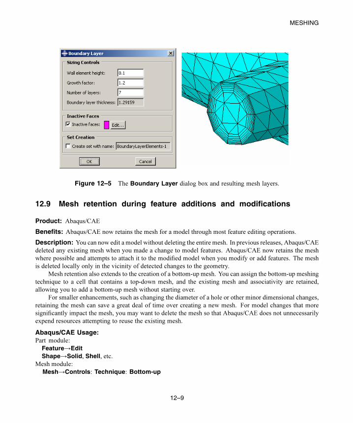
MESHING
Figure 12–5 The Boundary Layer dialog box and resulting mesh layers.
12.9 Mesh retention during feature additions and modifications
Product: Abaqus/CAE
Benefits: Abaqus/CAE now retains the mesh for a model through most feature editing operations.
Description: You can now edit a model without deleting the entire mesh. In previous releases, Abaqus/CAE
deleted any existing mesh when you made a change to model features. Abaqus/CAE now retains the mesh
where possible and attempts to attach it to the modified model when you modify or add features. The mesh
is deleted locally only in the vicinity of detected changes to the geometry.
Mesh retention also extends to the creation of a bottom-up mesh. You can assign the bottom-up meshing
technique to a cell that contains a top-down mesh, and the existing mesh and associativity are retained,
allowing you to add a bottom-up mesh without starting over.
For smaller enhancements, such as changing the diameter of a hole or other minor dimensional changes,
retaining the mesh can save a great deal of time over creating a new mesh. For model changes that more
significantly impact the mesh, you may want to delete the mesh so that Abaqus/CAE does not unnecessarily
expend resources attempting to reuse the existing mesh.
Abaqus/CAE Usage:Part module:
Feature→EditShape→Solid, Shell, etc.
Mesh module:
Mesh→Controls: Technique: Bottom-up
12–9
Abaqus ID:
Printed on:

MESHING
References:
Abaqus/CAE User’s Manual
• “Adding a feature to a part,” Section 11.20, in the online HTML version of this manual
• “Using the Edit Feature dialog box,” Section 11.25, in the online HTML version of this manual
• “Bottom-up meshing,” Section 17.11
12–10
Abaqus ID:
Printed on:
EXECUTION
13. Execution
This chapter discusses commands and utilities for running the Abaqus products. It provides an overview of
the following enhancements:
• “Parallel execution of the element operations,” Section 13.1
• “Parallel execution in the analysis input file processor,” Section 13.2
• “Multiple GPGPUs supported in the direct sparse solver,” Section 13.3
• “Translating LS-DYNA input files to partial Abaqus input files,” Section 13.4
13.1 Parallel execution of the element operations
Product: Abaqus/Standard
Benefits: The analysis time of certain procedures is reduced by parallel execution of the element operations.
Description: Thread-based parallel execution of the element operations is now supported for the following
linear perturbation procedures:
• natural frequency extraction that uses the SIM architecture,
• modal linear dynamic analyses that use the SIM architecture,
• substructure generation, and
• matrix generation.
References:
Abaqus Analysis User’s Manual
• “Parallel execution in Abaqus/Standard,” Section 3.5.2
• “Natural frequency extraction,” Section 6.3.5
• “Complex eigenvalue extraction,” Section 6.3.6
• “Transient modal dynamic analysis,” Section 6.3.7
• “Mode-based steady-state dynamic analysis,” Section 6.3.8
• “Subspace-based steady-state dynamic analysis,” Section 6.3.9
• “Defining substructures,” Section 10.1.2
• “Generating matrices,” Section 10.3.1
13.2 Parallel execution in the analysis input file processor
Product: Abaqus/Standard
13–1
Abaqus ID:
Printed on:
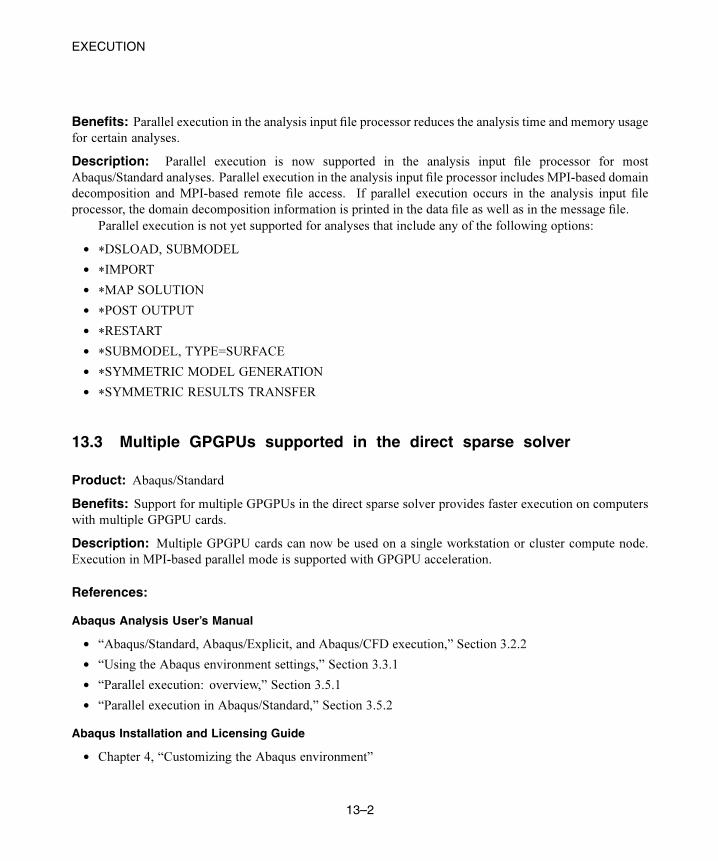
EXECUTION
Benefits: Parallel execution in the analysis input file processor reduces the analysis time and memory usage
for certain analyses.
Description: Parallel execution is now supported in the analysis input file processor for most
Abaqus/Standard analyses. Parallel execution in the analysis input file processor includes MPI-based domain
decomposition and MPI-based remote file access. If parallel execution occurs in the analysis input file
processor, the domain decomposition information is printed in the data file as well as in the message file.
Parallel execution is not yet supported for analyses that include any of the following options:
• *DSLOAD, SUBMODEL
• *IMPORT
• *MAP SOLUTION
• *POST OUTPUT
• *RESTART
• *SUBMODEL, TYPE=SURFACE
• *SYMMETRIC MODEL GENERATION
• *SYMMETRIC RESULTS TRANSFER
13.3 Multiple GPGPUs supported in the direct sparse solver
Product: Abaqus/Standard
Benefits: Support for multiple GPGPUs in the direct sparse solver provides faster execution on computers
with multiple GPGPU cards.
Description: Multiple GPGPU cards can now be used on a single workstation or cluster compute node.
Execution in MPI-based parallel mode is supported with GPGPU acceleration.
References:
Abaqus Analysis User’s Manual
• “Abaqus/Standard, Abaqus/Explicit, and Abaqus/CFD execution,” Section 3.2.2
• “Using the Abaqus environment settings,” Section 3.3.1
• “Parallel execution: overview,” Section 3.5.1
• “Parallel execution in Abaqus/Standard,” Section 3.5.2
Abaqus Installation and Licensing Guide
• Chapter 4, “Customizing the Abaqus environment”
13–2
Abaqus ID:
Printed on:
EXECUTION
13.4 Translating LS-DYNA input files to partial Abaqus input files
Product: Abaqus/Explicit
Benefits: You can now translate an LS-DYNA keyword file to a partial Abaqus input file.
Description: The new abaqus fromdyna execution procedure enables you to convert an LS-DYNA analysis
model to an Abaqus equivalent.
Reference:
Abaqus Analysis User’s Manual
• “Translating LS-DYNA data files to Abaqus input files,” Section 3.2.30
13–3
Abaqus ID:
Printed on:

OUTPUT AND VISUALIZATION
14. Output and visualization
This chapter discusses obtaining, postprocessing, and visualizing results from Abaqus analyses. It provides
an overview of the following enhancements:
• “Requesting field output on exterior nodes and elements in Abaqus/CAE,” Section 14.1
• “Displaying multiple slices of view cut data,” Section 14.2
• “Enhancements to free body display,” Section 14.3
• “Editing free body cuts,” Section 14.4
• “Selecting elements by topology in the Visualization module,” Section 14.5
• “Enhancement to material orientation plot display,” Section 14.6
• “Nodal field output for tie constraints,” Section 14.7
• “Maximum damage initiation output for shells,” Section 14.8
• “Air blast pressure load output,” Section 14.9
• “Shear rate and viscosity field output available in Abaqus/CFD,” Section 14.10
• “EXODUS-II and NEMESIS output for Abaqus/CFD field output,” Section 14.11
• “Reading X–Y data from history output based on the step time,” Section 14.12
• “Filtering selections for results output,” Section 14.13
14.1 Requesting field output on exterior nodes and elements inAbaqus/CAE
Product: Abaqus/CAE
Benefits: In Abaqus/CAE you can now easily request field output on the exterior nodes and elements of a
model, which reduces the size of the output database and is particularly useful for visualization of the overall
deformation of the model.
Description: For three-dimensional models in Abaqus/Standard and Abaqus/Explicit analyses, you can
request field output on the exterior nodes and elements, as shown in Figure 14–1.
Abaqus/CAE Usage:Step module:
Field output request editor: Domain: Whole model; toggle on Exterior only
References:
Abaqus Analysis User’s Manual
• “Output to the output database,” Section 4.1.3
14–1
Abaqus ID:
Printed on:
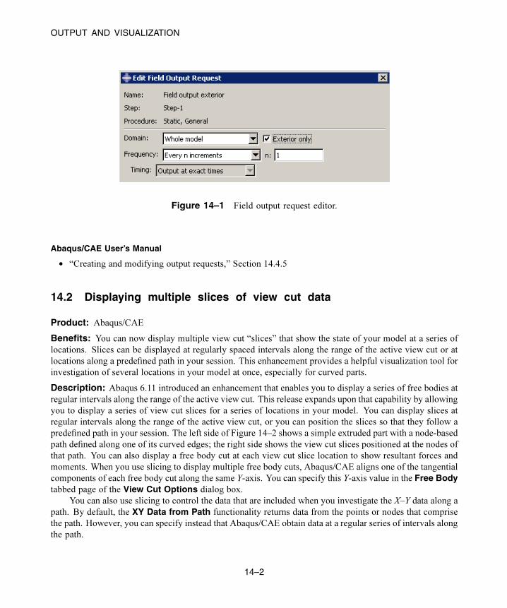
OUTPUT AND VISUALIZATION
Figure 14–1 Field output request editor.
Abaqus/CAE User’s Manual
• “Creating and modifying output requests,” Section 14.4.5
14.2 Displaying multiple slices of view cut data
Product: Abaqus/CAE
Benefits: You can now display multiple view cut “slices” that show the state of your model at a series of
locations. Slices can be displayed at regularly spaced intervals along the range of the active view cut or at
locations along a predefined path in your session. This enhancement provides a helpful visualization tool for
investigation of several locations in your model at once, especially for curved parts.
Description: Abaqus 6.11 introduced an enhancement that enables you to display a series of free bodies at
regular intervals along the range of the active view cut. This release expands upon that capability by allowing
you to display a series of view cut slices for a series of locations in your model. You can display slices at
regular intervals along the range of the active view cut, or you can position the slices so that they follow a
predefined path in your session. The left side of Figure 14–2 shows a simple extruded part with a node-based
path defined along one of its curved edges; the right side shows the view cut slices positioned at the nodes of
that path. You can also display a free body cut at each view cut slice location to show resultant forces and
moments. When you use slicing to display multiple free body cuts, Abaqus/CAE aligns one of the tangential
components of each free body cut along the same Y-axis. You can specify this Y-axis value in the Free Bodytabbed page of the View Cut Options dialog box.
You can also use slicing to control the data that are included when you investigate the X–Y data along a
path. By default, the XY Data from Path functionality returns data from the points or nodes that comprise
the path. However, you can specify instead that Abaqus/CAE obtain data at a regular series of intervals along
the path.
14–2
Abaqus ID:
Printed on:
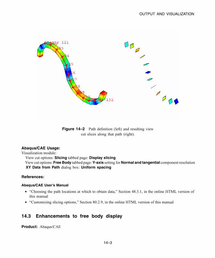
OUTPUT AND VISUALIZATION
Figure 14–2 Path definition (left) and resulting view
cut slices along that path (right).
Abaqus/CAE Usage:Visualization module:
View cut options: Slicing tabbed page: Display slicingView cut options:Free Body tabbed page:Y-axis setting forNormal and tangential component resolution
XY Data from Path dialog box: Uniform spacing
References:
Abaqus/CAE User’s Manual
• “Choosing the path locations at which to obtain data,” Section 48.3.1, in the online HTML version of
this manual
• “Customizing slicing options,” Section 80.2.9, in the online HTML version of this manual
14.3 Enhancements to free body display
Product: Abaqus/CAE
14–3
Abaqus ID:
Printed on:
OUTPUT AND VISUALIZATION
Benefits: You can now display free body data for nonplanar view cuts, which enables you to investigate
resultant forces and moments for regions in which planar view cuts are not suitable. In addition, free body cut
labels are now displayed in a smaller font, which improves legibility for tasks in which you want to investigate
resultant forces and moments in a greater number of locations.
Description: Abaqus/CAE now enables you to display resultant forces and moments for cylindrical view
cuts, spherical view cuts, and isosurface view cuts. In earlier releases this functionality was limited to planar
view cuts only.
In addition, Abaqus/CAE now uses a smaller font size for displaying the labels on a free body cut. The
smaller size helps you to display a greater number of free body cuts without the labels obscuring each other
or covering portions of the model.
Reference:
Abaqus/CAE User’s Manual
• “Displaying a cut section and its resultant force andmoment vectors,” Section 80.2.2, in the online HTML
version of this manual
14.4 Editing free body cuts
Product: Abaqus/CAE
Benefits: Abaqus/CAE now enables you to edit any of the free body cuts in your session.
Description: When you edit a free body cut, you cannot edit the selection method that was used as part of
its definition, but you can change the following aspects of its definition:
• You can edit the set of edges, faces, or nodes and elements that define the free body cross-section. When
you change the free body cross-section, Abaqus/CAE customizes the default selection item and method
in the Free Body Cross-Section dialog box so that they match the settings that were selected the last
time you edited the free body cut. For example, if you specified the free body cross-section by selecting
a group of surface sets, the default selection item will be Surfaces and the default selection method will
be Surface sets.
• You can change the settings for the summation point of the resultant force and moment vectors and
change the component resolution options when vectors are displayed in component form. These options,
specified in the Edit Free Body Cut dialog box, are also customized so that their default values match
the most recently selected options for this free body cut.
Abaqus/CAE Usage:Visualization module:
Tools→Free Body→Edit→free body name
14–4
Abaqus ID:
Printed on:
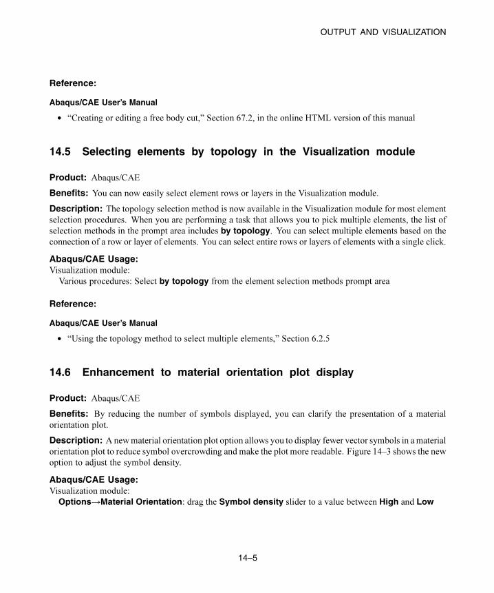
OUTPUT AND VISUALIZATION
Reference:
Abaqus/CAE User’s Manual
• “Creating or editing a free body cut,” Section 67.2, in the online HTML version of this manual
14.5 Selecting elements by topology in the Visualization module
Product: Abaqus/CAE
Benefits: You can now easily select element rows or layers in the Visualization module.
Description: The topology selection method is now available in the Visualization module for most element
selection procedures. When you are performing a task that allows you to pick multiple elements, the list of
selection methods in the prompt area includes by topology. You can select multiple elements based on the
connection of a row or layer of elements. You can select entire rows or layers of elements with a single click.
Abaqus/CAE Usage:Visualization module:
Various procedures: Select by topology from the element selection methods prompt area
Reference:
Abaqus/CAE User’s Manual
• “Using the topology method to select multiple elements,” Section 6.2.5
14.6 Enhancement to material orientation plot display
Product: Abaqus/CAE
Benefits: By reducing the number of symbols displayed, you can clarify the presentation of a material
orientation plot.
Description: A newmaterial orientation plot option allows you to display fewer vector symbols in a material
orientation plot to reduce symbol overcrowding and make the plot more readable. Figure 14–3 shows the new
option to adjust the symbol density.
Abaqus/CAE Usage:Visualization module:
Options→Material Orientation: drag the Symbol density slider to a value between High and Low
14–5
Abaqus ID:
Printed on:
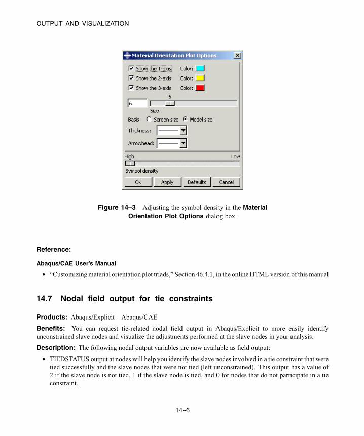
OUTPUT AND VISUALIZATION
Figure 14–3 Adjusting the symbol density in the MaterialOrientation Plot Options dialog box.
Reference:
Abaqus/CAE User’s Manual
• “Customizingmaterial orientation plot triads,” Section 46.4.1, in the online HTML version of this manual
14.7 Nodal field output for tie constraints
Products: Abaqus/Explicit Abaqus/CAE
Benefits: You can request tie-related nodal field output in Abaqus/Explicit to more easily identify
unconstrained slave nodes and visualize the adjustments performed at the slave nodes in your analysis.
Description: The following nodal output variables are now available as field output:
• TIEDSTATUS output at nodes will help you identify the slave nodes involved in a tie constraint that were
tied successfully and the slave nodes that were not tied (left unconstrained). This output has a value of
2 if the slave node is not tied, 1 if the slave node is tied, and 0 for nodes that do not participate in a tie
constraint.
14–6
Abaqus ID:
Printed on:
OUTPUT AND VISUALIZATION
• TIEADJUST vector output at slave nodes will help you visualize the adjustment performed at the slave
nodes involved in a tie constraint where all tied nodes on the slave surface are moved onto the master
surface in the initial configuration without any strain.
Abaqus/CAE Usage:Step module:
Field output request editor: Output Variables: State/Field/User/Time: TIEDSTATUS and TIEADJUST
References:
Abaqus Analysis User’s Manual
• “Abaqus/Explicit output variable identifiers,” Section 4.2.2
• “Mesh tie constraints,” Section 34.3.1
Abaqus/CAE User’s Manual
• “Creating and modifying output requests,” Section 14.4.5
14.8 Maximum damage initiation output for shells
Products: Abaqus/Explicit Abaqus/CAE
Benefits: New damage initiation output is now available in Abaqus/Explicit to improve capturing the results
of your analysis.
Description: The following damage initiation field element output variables are now available:
• DMICRTMAX element output generates three element output quantities:
– DMICRTMAXVAL, maximum damage initiation value
– DMICRTTYPE, damage initiation type for which the maximum damage initiation was reached
– DMICRTPOS, section point number in the beam or shell section for which the maximum damage
initiation was reached; for solid elements, this value is one.
• EDMICRTMAX whole shell element output generates four output quantities:
– EDMICRTMAXVAL, maximum damage initiation value
– EDMICRTLAYER, damage initiation layer for which the maximum damage initiation value
occurred
– EDMICRTTYPE, damage initiation type for which the maximum damage initiation was reached
– EDMICRTINTP, integration point number for which the maximum damage initiation was reached;
for reduced-integration elements, this value is one.
Abaqus/CAE Usage:Step module:
Field output request editor: Output Variables: Failure/Fracture: DMICRTMAX and EDMICRTMAX
14–7
Abaqus ID:
Printed on:
OUTPUT AND VISUALIZATION
References:
Abaqus Analysis User’s Manual
• “Abaqus/Explicit output variable identifiers,” Section 4.2.2
Abaqus/CAE User’s Manual
• “Creating and modifying output requests,” Section 14.4.5
14.9 Air blast pressure load output
Products: Abaqus/Explicit Abaqus/CAE
Benefits: The incident wave pressure field output for shock waves using the CONWEP model is now
available in Abaqus/Explicit.
Description: Pressure loading due to an incident shock wave caused by an air explosion is calculated using
the CONWEP model in Abaqus/Explicit. The new element field output variable IWCONWEP can now be
requested on the element faces on which you apply this type of pressure load.
Abaqus/CAE Usage:Step module:
Field output request editor: Output Variables: Forces/Reactions: IWCONWEP
References:
Abaqus Analysis User’s Manual
• “Abaqus/Explicit output variable identifiers,” Section 4.2.2
• “Defining air blast loading for incident shock waves using the CONWEP model in Abaqus/Explicit” in
“Acoustic and shock loads,” Section 33.4.6
Abaqus/CAE User’s Manual
• “Creating and modifying output requests,” Section 14.4.5
14.10 Shear rate and viscosity field output available in Abaqus/CFD
Product: Abaqus/CFD
Benefits: Shear rate output and viscosity element field output are now available in Abaqus/CFD to visualize
engineering shear strain rates and spatially varying viscosities in non-Newtonian flows.
Description: The following field output variables are now available in an Abaqus/CFD analysis for
improved visualization in non-Newtonian flows:
14–8
Abaqus ID:
Printed on:
OUTPUT AND VISUALIZATION
• SHEARRATE, element and nodal field output to visualize engineering shear strain rates
• VISCOSITY, element field output can be requested at the element centers to visualize spatially varying
viscosities
Reference:
Abaqus Analysis User’s Manual
• “Output,” Section 4.1.1
14.11 EXODUS-II and NEMESIS output for Abaqus/CFD field output
Product: Abaqus/CFD
Benefits: Field output from an Abaqus/CFD analysis is now available for the EXODUS-II and NEMESIS
output formats. These output formats allow for postprocessing results from serial or parallel jobs using third-
party visualizers (e.g., ParaView).
Description: The new EXODUS-II and NEMESIS output is available for all existing field output requests
and is activated using the command line option -field with the value exodus or nemesis.
Reference:
Abaqus Analysis User’s Manual
• “Output,” Section 4.1.1
14.12 Reading X–Y data from history output based on the step time
Product: Abaqus/CAE
Benefits: You can now select the step time as the basis for reading X–Y data from history output in an output
database to improve usability in multistep analyses.
Description: When reading X–Y data from history output for time-based analyses, X-values are taken as
total time from the start of the analysis or, in the case of a restarted analysis, as total time from the start of
the last continuation of the analysis. You can now use the step time as the time basis. This enhancement is
beneficial for multistep analyses; for example, when there is a difference in the order of magnitude of the step
times. You can reduce the number of operations required on X–Y data; for example, if you want to create a
smooth curve using data from Step 2 and Step 5 in a 7-step analysis.
Abaqus/CAE Usage:Visualization module:
Result→History Output: Steps/Frames tabbed page, toggle on Use Step Time
14–9
Abaqus ID:
Printed on:
OUTPUT AND VISUALIZATION
Reference:
Abaqus/CAE User’s Manual
• “Reading X–Y data from output database history output,” Section 47.2.1
14.13 Filtering selections for results output
Product: Abaqus/CAE
Benefits: New filters for results output improve handling of results data for postprocessing complex parts,
particularly composite parts.
Description: You can now filter ply selections by name when you select section point data by ply for
integration point results and material orientations to simplify ply selection in models containing very large
ply stacks. A new name filter has also been added for selecting a user-specified coordinate system (defined
either during model generation or during postprocessing) for a transformation.
Abaqus/CAE Usage:Visualization module:
Result→Section Points: Selection method: Plies, Name filterResult→Options: Transformation tabbed page; Transform Type: User-specified, Name filter
References:
Abaqus/CAE User’s Manual
• “Selecting section point data,” Section 42.5.9, in the online HTML version of this manual
• “Transforming results into a new coordinate system,” Section 42.6.8, in the online HTML version of this
manual
14–10
Abaqus ID:
Printed on:
USER SUBROUTINES, UTILITIES, AND PLUG-INS
15. User subroutines, utilities, and plug-ins
This chapter discusses additional user programs that can be run with Abaqus. It provides an overview of the
following enhancements:
• “Enhancements to user subroutines UAMP and VUAMP,” Section 15.1
• “User subroutine to define damage behavior with Mullins effect in Abaqus/Explicit,” Section 15.2
• “User subroutines for pressure and velocity boundary conditions in Abaqus/CFD,” Section 15.3
• “Enhancements for defining nonuniform magnetic vector potential and nonuniform current density,”
Section 15.4
15.1 Enhancements to user subroutines UAMP and VUAMP
Products: Abaqus/Standard Abaqus/Explicit
Benefits: You can now define user amplitude properties directly within the input file that calls the user
subroutine rather than having to define properties within the user subroutine itself. This new feature allows
for a smoother workflow in that the user subroutine no longer has to be modified each time an amplitude
property is changed.
Description: User subroutines UAMP and VUAMP have been modified so that amplitude properties can be
read in from the input file that calls the user subroutine. The new PROPERTIES parameter allows multiple
amplitude properties to be defined on the data lines of user amplitude definitions.
References:
Abaqus Analysis User’s Manual
• “Amplitude curves,” Section 33.1.2
Abaqus Keywords Reference Manual
• *AMPLITUDE
Abaqus User Subroutines Reference Manual
• “UAMP,” Section 1.1.19
• “VUAMP,” Section 1.2.7
Abaqus Example Problems Manual
• “Crank mechanism,” Section 4.1.2
Abaqus Verification Manual
• “VUAMP,” Section 4.1.31
15–1
Abaqus ID:
Printed on:
USER SUBROUTINES, UTILITIES, AND PLUG-INS
15.2 User subroutine to define damage behavior with Mullins effectin Abaqus/Explicit
Product: Abaqus/Explicit
Benefits: You can now define the damage behavior associated withMullins effect (stress softening of certain
filled elastomers) in Abaqus/Explicit. This feature was previously available only in Abaqus/Standard.
Description: User subroutine VUMULLINS can be used to define the damage variable associated with
Mullins effect in Abaqus/Explicit. This feature provides functionality equivalent to user subroutine
UMULLINS in Abaqus/Standard. The feature complements the two other available methods for defining
damage; namely, direct specification of damage material parameters or specification of test data. The
damage can be defined in terms of any number of user-defined constants. The subroutine also provides users
with access to solution-dependent state variables as well as temperature and field variables. In addition to
defining the damage variable, the user can also define the strain energy dissipation due to damage as well
as a criterion for material failure.
References:
Abaqus Analysis User’s Manual
• “Mullins effect,” Section 22.6.1
• “Energy dissipation in elastomeric foams,” Section 22.6.2
Abaqus Keywords Reference Manual
• *MULLINS EFFECT
Abaqus User Subroutines Reference Manual
• “VUMULLINS,” Section 1.2.18
Abaqus Verification Manual
• “Mullins effect and permanent set,” Section 2.2.3
15.3 User subroutines for pressure and velocity boundary conditionsin Abaqus/CFD
Product: Abaqus/CFD
Benefits: You can now define pressure and velocity boundary conditions in Abaqus/CFD.
Description: User subroutines for pressure and velocity boundary conditions are now available in
Abaqus/CFD. New user subroutine utilities have been added as well to provide the current simulation state
and other additional useful input to the user subroutine developer.
15–2
Abaqus ID:
Printed on:
USER SUBROUTINES, UTILITIES, AND PLUG-INS
References:
Abaqus Analysis User’s Manual
• “Boundary conditions in Abaqus/CFD,” Section 33.3.2
Abaqus Keywords Reference Manual
• *FLUID BOUNDARY
Abaqus User Subroutines Reference Manual
• “SMACfdUserPressureBC,” Section 1.3.1
• “SMACfdUserVelocityBC,” Section 1.3.2
• “Obtaining scalar state information in an Abaqus/CFD analysis,” Section 2.1.19
• “Obtaining vector state information in an Abaqus/CFD analysis,” Section 2.1.20
• “Obtaining the MPI communicator in an Abaqus/CFD analysis,” Section 2.1.21
15.4 Enhancements for defining nonuniform magnetic vector potentialand nonuniform current density
Product: Abaqus/Standard
Benefits: User subroutines UDEMPOTENTIAL, UDECURRENT, and UDSECURRENT can now be used in
transient eddy current and magnetostatic analyses.
Description: Previously available in time-harmonic eddy current analyses, you can now define
nonuniform magnetic vector potential on a surface (UDEMPOTENTIAL), nonuniform volume current
density (UDECURRENT), and nonuniform surface current density (UDSECURRENT) in transient eddy current
and magnetostatic analyses. For more information, see “Magnetostatic analysis in Abaqus/Standard,”
Section 4.5, and “Transient eddy current analysis in Abaqus/Standard,” Section 4.6.
References:
Abaqus Analysis User’s Manual
• “Eddy current analysis,” Section 6.7.5
• “Magnetostatic analysis,” Section 6.7.6
Abaqus User Subroutines Reference Manual
• “UDECURRENT,” Section 1.1.23
• “UDEMPOTENTIAL,” Section 1.1.24
• “UDSECURRENT,” Section 1.1.26
15–3
Abaqus ID:
Printed on:

Abaqus SCRIPTING INTERFACE
16. Abaqus Scripting Interface
This chapter discusses using the Abaqus Scripting Interface to write user scripts. Abaqus makes every attempt
to be backward compatible and can execute most Abaqus Scripting Interface scripts from previous releases
of Abaqus. However, backward compatibility is not guaranteed beyond several releases of Abaqus, and it
is recommended that you upgrade your commands to the most recent release. A complete list of Abaqus
Scripting Interface commands that have changed is included in in the Abaqus Scripting Reference Manual.
This chapter provides an overview of the following enhancements:
• “Expanded object coverage for definition of custom kernel data,” Section 16.1
• “Descriptive header in the journal file,” Section 16.2
• “Abaqus PDE improvements,” Section 16.3
• “Skipping the last command during session recovery,” Section 16.4
• “Faster tab completion,” Section 16.5
• “Selected errors now classified as an AbaqusExceptionType,” Section 16.6
• “Better control over writing messages to the journal file,” Section 16.7
• “Reformatting commands in Python files with proper indentation,” Section 16.8
• “Improved message handling and reporting of plug-ins,” Section 16.9
• “Stop button for scripts,” Section 16.10
16.1 Expanded object coverage for definition of custom kernel data
Products: Abaqus/Standard Abaqus/Explicit Abaqus/CAE
Benefits: You can now store custom data for many of the objects within an Abaqus/CAE model database;
this functionality was previously available only for the Mdb object. This enhancement enables you to store
the data associated with custom classes and functions in the specific objects to which these data pertain.
Description: The customKernel module is now available for use in the following objects in an
Abaqus/CAE model database:
• Amplitude
• Assembly
• BoundaryCondition
• ConstrainedSketch
• Interaction
• InteractionProperty
• Job
• Load
16–1
Abaqus ID:
Printed on:
Abaqus SCRIPTING INTERFACE
• Material
• Model
• Part
• PartInstance
• Repository
• Section
• Step
Reference:
Abaqus Scripting User’s Manual
• “Storing custom data in the model database or in other objects,” Section 5.6.1
16.2 Descriptive header in the journal file
Products: Abaqus/Standard Abaqus/Explicit Abaqus/CAE
Benefits: The journal file now includes a header section that provides the Abaqus version, model database
version, and the date when the model database was last saved. This information can be helpful when you
recreate a saved model database.
Description: The journal (.jnl) file contains the Abaqus/CAE commands that will replicate the model
database that was saved to disk. This file now includes a header section that describes the following: the
Abaqus version, model database version, and the date when the model database was last saved.
Reference:
Abaqus Scripting User’s Manual
• “Recreating a saved model database,” Section 9.5.2
16.3 Abaqus PDE improvements
Product: Abaqus/CAE
Benefits: When you navigate to the file you want to open in the Abaqus PDE, you can now specify its path
using environment variables for faster navigation. In addition, search functionality uses a default setting of
exact matches.
Description: You can now navigate to the file you want to open in the Select File dialog box by specifying
an environment variable in the File Name field. In addition, your searches of the main file now return matches
that ignore case by default rather than returning only exact matches.
16–2
Abaqus ID:
Printed on:
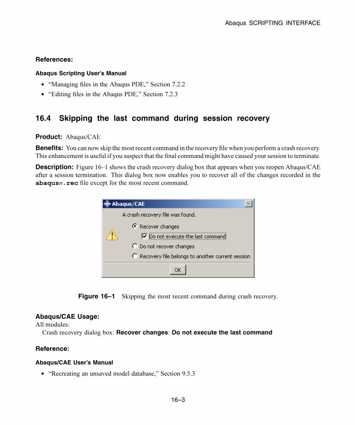
Abaqus SCRIPTING INTERFACE
References:
Abaqus Scripting User’s Manual
• “Managing files in the Abaqus PDE,” Section 7.2.2
• “Editing files in the Abaqus PDE,” Section 7.2.3
16.4 Skipping the last command during session recovery
Product: Abaqus/CAE
Benefits: You can now skip the most recent command in the recovery file when you perform a crash recovery.
This enhancement is useful if you suspect that the final command might have caused your session to terminate.
Description: Figure 16–1 shows the crash recovery dialog box that appears when you reopen Abaqus/CAE
after a session termination. This dialog box now enables you to recover all of the changes recorded in the
abaqusn.rec file except for the most recent command.
Figure 16–1 Skipping the most recent command during crash recovery.
Abaqus/CAE Usage:All modules:
Crash recovery dialog box: Recover changes: Do not execute the last command
Reference:
Abaqus/CAE User’s Manual
• “Recreating an unsaved model database,” Section 9.5.3
16–3
Abaqus ID:
Printed on:

Abaqus SCRIPTING INTERFACE
16.5 Faster tab completion
Product: Abaqus/CAE
Benefits: The interactive Python interfaces in Abaqus/CAE and the Abaqus PDE now provide faster tab
completion performance when you have a large number of items in your path.
Description: In earlier Abaqus releases, tab completion in the interactive Python interfaces was sometimes
slow when the Python sys.path included several network locations. Abaqus 6.12 now provides a threaded
directory search that offers faster performance even when you have a large number of network locations in
your path.
Reference:
Abaqus Scripting User’s Manual
• “Using tab completion to explore the object model,” Section 6.1.2
16.6 Selected errors now classified as an AbaqusExceptionType
Benefits: AbaqusException errors are now classified as an AbaqusExceptionType. This
classification provides a more descriptive grouping for errors.
Description: The Python type of an AbaqusException has changed from MetaClassPrint to
AbaqusExceptionType.
Reference:
Abaqus Scripting User’s Manual
• “Error handling in the Abaqus Scripting Interface,” Section 5.5
16.7 Better control over writing messages to the journal file
Benefits: The Abaqus GUI Toolkit has been updated to enable you to control whether messages are written
to the journal file.
Description: The writeToJournal argument is now available for many methods in the Abaqus GUI Toolkit.
You can set this argument to True to write commands to the message file for the selected method.
In addition, you can run the journalMethodCall function to record a command in the journal file.
This option is preferable to the use of the writeToJournal argument if you write your own kernel scripting
module and functions. Your command should not call journalMethodCall if the command changes the
Mdb object using built-in Abaqus Scripting Interface commands, because these are journaled by default. Your
command should call journalMethodCall if the command changes the customData object in the model
16–4
Abaqus ID:
Printed on:
Abaqus SCRIPTING INTERFACE
database. For more information, see “Executing commands,” Section 6.3 in the Abaqus GUI Toolkit User’s
Manual.
16.8 Reformatting commands in Python files with proper indentation
Benefits: Abaqus now includes a utility that enables you to reformat a Python file with standard indentation.
This release also provides proper indentation for commands in the replay file that are generated by the recovery
file.
Description: The redentABQ.py utility re-indents a Python source file by adjusting the leading white
space in front of Python commands and in front of comments.
When you perform a recovery, Abaqus now provides improved indentation for the entries in a replay
(.rpy) file that are generated from the recovery (.rec) file.
Reference:
Abaqus Scripting Reference Manual
• “redentABQ module,” Section 52.1
16.9 Improved message handling and reporting of plug-ins
Product: Abaqus/CAE
Benefits: You can now display exceptions associated with the import of plug-ins when you start
Abaqus/CAE.
Description: By default, Abaqus/CAE does not display the exceptions associated with the import of plug-ins
when you start the application. If you want to expose these exceptions for debugging purposes, set the
environment variable ABQ_PLUGIN_DEBUG to 1 at a command prompt before launching Abaqus/CAE.
When this environment variable is set, Abaqus/CAE provides more trackback information about plug-ins
upon startup, including the location and nature of any failures that occur.
Reference:
Abaqus/CAE User’s Manual
• “Displaying exceptions for imported plug-ins at startup,” Section 81.11
16.10 Stop button for scripts
Product: Abaqus/CAE
Benefits: You can now click a button to stop execution of a Python script in Abaqus/CAE.
16–5
Abaqus ID:
Printed on:
Abaqus SCRIPTING INTERFACE
Description: The showStopButtonInGui command enables you to display a stop button in
Abaqus/CAE when the running time for a Python script has exceeded a duration specified in the calling
script. Abaqus/CAE issues this command automatically when a command is entered from the command line
interface (CLI), as part of a macro, or from the File→Run Script menu option. The command is not issued
automatically when a Python script is run from the user interface—for example, as part of a plug-in—but
you can run it from the CLI or from a command prompt.
Reference:
Abaqus Scripting User’s Manual
• “Executing scripts,” Section 5.1
16–6
Abaqus ID:
Printed on:
SUMMARY OF CHANGES
17. Summary of changes
This section summarizes the changes and the additions that have been made to the items that define an
Abaqus model, including keywords, user subroutines, and output variables. For more information on these
modifications, refer to the preceding chapters.
The following identifiers are used:
new New in Abaqus 6.12.
mod Existed in Abaqus 6.11 but has been modified or enhanced in Abaqus 6.12.
(S) New, modified, or removed in Abaqus/Standard.
(E) New, modified, or removed in Abaqus/Explicit.
(C) New, modified, or removed in Abaqus/CFD.
17.1 Changes in Abaqus options
This section summarizes the changes and the additions that have been made to the options that define an
Abaqus model.
new (E) *ADAPTIVE MESH REFINEMENT
Activate adaptive mesh refinement in an Eulerian domain.
mod (S)(E) *AMPLITUDE
Use the new PROPERTIES parameter to specify the number of user amplitude
properties that are defined either on the data lines or directly within user subroutine
UAMP or VUAMP.
mod (S) *BEAM SECTION
A new section type is available. Set SECTION=THICK PIPE to define a thick-
walled circular section.
mod (S) *BOUNDARY
Use the new PHANTOM parameter to apply boundary conditions to a phantom
node that is originally located coincident with the specified real node in an enriched
element.
mod (S) *CAP CREEP
Use the new TIME parameter to specify whether creep time or total time is used in
the time-hardening and Singh-Mitchell relations.
17–1
Abaqus ID:
Printed on:
SUMMARY OF CHANGES
mod (C) *CFD
The maximum allowable time increment and the time weight for the advective
terms in the momentum and scalar transport equations can now be specified on the
data lines.
mod (S) *CONNECTOR DAMPING
Use the new UNSYMM and FREQUENCY DEPENDENCE parameters to define
unsymmetric and/or frequency-dependent linear coupled viscous damping matrices,
respectively.
mod (S) *CONNECTOR ELASTICITY
Use the new UNSYMM and FREQUENCY DEPENDENCE parameters to
define unsymmetric and/or frequency-dependent linear coupled stiffness matrices,
respectively.
mod (S) *CONTACT PAIR
The ADJUST parameter can now be used for self-contact.
mod (S) *CONTROLS
A new data entry has been added to this option when TYPE=FSI is used. This data
entry can be used to define the solid/fluid density ratio to control the FSI stabilization.
mod (S) *CREEP
Use the new TIME parameter to specify whether creep time or total time is used in
the time-hardening relation.
mod (S) *D EM POTENTIAL
This option is now available in transient eddy current and magnetostatic analyses.
mod (E) *DAMAGE INITIATION
Use the new LODE DEPENDENT parameter in conjunction with
CRITERION=DUCTILE to define the equivalent plastic strain at the onset of
ductile damage as a function of the Lode angle.
mod (E) *DAMPING
The ALPHA parameter can now take the value TABULAR to define temperature
and/or field-dependent mass proportional damping.
The BETA parameter can now take the value TABULAR to define temperature
and/or field-dependent stiffness proportional damping.
Use the new DEPENDENCIES parameter to define the number of field variables
when ALPHA=TABULAR and/or BETA=TABULAR.
mod (S) *DEBOND
The DEBONDING FORCE parameter can now be used with TYPE=ENHANCED
VCCT.
17–2
Abaqus ID:
Printed on:
SUMMARY OF CHANGES
mod (S) *DECURRENT
This option is now available in transient eddy current and magnetostatic analyses.
mod (E) *DEPVAR
Use the new CONVERT parameter to support user subroutine–based conversion of
finite elements to SPH particles.
mod (C) *DISTRIBUTION
A new value is available for the LOCATION parameter. Set LOCATION=NONE to
define a distribution used with a fluid boundary condition.
mod (C) *DISTRIBUTION TABLE
Labels for PRESSURE and VOLUME to define a distribution table for pressure that
varies with the total volume of fluid crossing a surface can now be specified on the
data line.
mod (S)(C) *DLOAD
Use the new load type ROTDYNF to define rotordynamic loads in an
Abaqus/Standard analysis.
Use the new load type PDBF to define a porous drag body force load in an
Abaqus/CFD analysis.
mod (S) *DRUCKER PRAGER CREEP
Use the new TIME parameter to specify whether creep time or total time is used in
the time-hardening and Singh-Mitchell relations.
mod (S) *DSECURRENT
This option is now available in transient eddy current and magnetostatic analyses.
mod (S) *ELECTROMAGNETIC
Use the new DIRECT parameter to select direct user control of the incrementation
through the step.
Use the new STABILIZATION parameter to stabilize the solution when the overall
system of equations may be ill conditioned.
Use the new TRANSIENT parameter to carry out a transient eddy current analysis.
mod (C) *ENERGY OUTPUT
This option is now available in Abaqus/CFD analyses.
mod (S) *ENRICHMENT ACTIVATION
A new value is available for the ACTIVATE parameter. Set ACTIVATE=AUTO
OFF to deactivate the enriched feature automatically once all the pre-existing cracks
(or if there are no pre-existing cracks, all the allowable newly nucleated cracks) have
propagated through the boundary of the given enriched feature within the step.
17–3
Abaqus ID:
Printed on:
SUMMARY OF CHANGES
mod (C) *FLUID BOUNDARY
Use the new boundary condition type PASSIVEOUTFLOW to specify the passive
outflow.
Use the new boundary condition type PVDEP to specify pressure boundary
conditions that vary with the total volume of fluid crossing a surface.
Use the new DISTRIBUTION parameter to define a distribution used in conjunction
with the PVDEP boundary type.
new (C) *FLUID SECTION
Specify element properties for fluid and porous media elements.
mod (S)(E) *FRACTURE CRITERION
A new value is available for the TYPE parameter. Set TYPE=ENHANCED VCCT
to use the enhanced VCCT criterion in which the onset and growth of a crack can be
controlled by two different critical fracture energy release rates.
Use the new UNSTABLE GROWTH TOLERANCE parameter to specify the
tolerance within which the unstable crack propagation criterion must be satisfied
for multiple nodes at and ahead of the crack tip to be allowed to debond without the
cut back of increment size in one increment when the VCCT criterion is satisfied
for an unstable crack problem.
mod (S) *MAGNETIC PERMEABILITY
Use the new NONLINEAR parameter to define nonlinear magnetic behavior of an
electromagnetic medium.
new (S) *MAGNETOSTATIC
Magnetostatic response due to a known distribution of direct current.
mod (S)(E) *MASS
The ALPHA parameter is now supported in Abaqus/Explicit to define mass
proportional damping.
Use the new TYPE parameter to specify the point mass as isotropic or anisotropic.
Use the new ORIENTATION parameter to prescribe the principal directions of the
anisotropic mass tensor.
mod (S) *MATRIX ASSEMBLE
Use the new NSET parameter to remap matrix nodes.
mod (S) *MATRIX GENERATE
Use the new PUBLIC NODES parameter to specify which nodes will be visible at
the usage model.
17–4
Abaqus ID:
Printed on:
SUMMARY OF CHANGES
mod (C) *MOMENTUM EQUATION SOLVER
A new value is available for the TYPE parameter. Set TYPE=ILUFGMRES
to enable the Incomplete LU factorization preconditioned Flexible Generalized
Minimum Residual linear solver.
The numbers of restart vectors can now be specified on the data line.
mod (E) *MULLINS EFFECT
The USER parameter can now be used with user subroutine VUMULLINS in an
Abaqus/Explicit analysis.
new (S) *NONLINEAR BH
Specify nonlinear magnetic behavior of a soft magnetic material.
mod (C) *PERMEABILITY
This option is now available in Abaqus/CFD analyses.
Use the new INERTIAL DRAG COEFFICIENT parameter to specify the value of
the constant in the expression for the inertial drag coefficient, .
A new value is available for the TYPE parameter. Set TYPE=CARMAN KOZENY
to define permeability as a function of porosity through the Carman-Kozeny relation.
mod (E) *ROTARY INERTIA
The ALPHA parameter is now supported in Abaqus/Explicit to define stiffness
proportional damping.
mod (E) *SECTION CONTROLS
Use the new ELEMENT CONVERSION and CONVERSION CRITERION
parameters to support the conversion of finite elements to SPH particles.
Use the new KERNEL parameter to allow for different kernel interpolators in
conjunction with smoothed particle hydrodynamics.
mod (E) *SURFACE PROPERTY ASSIGNMENT
The PROPERTY=GEOMETRIC CORRECTION can now be used in
Abaqus/Explicit analyses.
mod (S) *SURFACE SMOOTHING
This option now allows the specification of surface smoothing on regions of surfaces
that correspond (or nearly correspond) to a toroidal surface.
mod (C) *TRANSPORT EQUATION SOLVER
A new value is available for the TYPE parameter. Set TYPE=ILUFGMRES
to enable the Incomplete LU factorization preconditioned Flexible Generalized
Minimum Residual linear solver.
The numbers of restart vectors can now be specified on the data line.
17–5
Abaqus ID:
Printed on:
SUMMARY OF CHANGES
mod (S)(E) *VISCOELASTIC
This option now allows the specification of viscoelastic properties for cohesive
elements with elastic traction-separation behavior in Abaqus/Explicit analyses.
Use the new NONLINEAR, LAW, NETWORKID, SRATIO, and DEPENDENCIES
parameters in an Abaqus/Standard analysis to define a nonlinear viscoelastic model
with multiple parallel networks.
mod (C) *VISCOSITY
This option is now available in the following shear rate–dependendent
non-Newtonian models: Carreau-Yasuda, Cross, Ellis-Meter, Herschel-Bulkley,
Powell-Eyring, and power law.
mod (S) *VISCOUS
Use the new TIME parameter to specify whether creep time or total time is used in
the time-hardening relation.
17.2 Changes in Abaqus user subroutines
This section summarizes the changes and the additions that have been made to user subroutines that can be
used in an Abaqus model.
mod (S) CREEP
The new variable TIME(3), value of creep time at the end of the increment, is
passed in for information.
mod (S) FRIC_COEF
Two variables that are passed in for information have been renamed: the average
current temperature between the master and slave surfaces at the contact point has
been renamed tempAvg(nBlock), and the average current value of all the user-
specified field variables between the master and slave surfaces at the contact point
has been renamed fieldAvg(nBlock,nFields).
new (C) SMACfdUserPressureBC
User subroutine to specify prescribed pressure boundary conditions.
new (C) SMACfdUserVelocityBC
User subroutine to specify prescribed velocity boundary conditions.
mod (S) UAMP
Two new variables can be passed in for information: props, user-specified array
of material constants associated with this amplitude definition, and nProps, user-
defined number of material constants associated with this amplitude definition.
17–6
Abaqus ID:
Printed on:
SUMMARY OF CHANGES
mod (S) UDECURRENT
A nonuniform volume current density vector can now be specified in transient eddy
current and magnetostatic analyses.
mod (S) UDEMPOTENTIAL
Surface-based nonuniform magnetic vector potential can now be specified in
transient eddy current and magnetostatic analyses.
mod (S) UDSECURRENT
A nonuniform surface current density vector can now be specified in transient eddy
current and magnetostatic analyses.
mod (E) VFRIC_COEF
Two variables that are passed in for information have been renamed: the average
current temperature between the master and slave surfaces at the contact point has
been renamed tempAvg(nBlock), and the average current value of all the user-
specified field variables between the master and slave surfaces at the contact point
has been renamed fieldAvg(nBlock,nFields).
mod (E) VUFIELD
Two changes were made to the variables passed in for information: the
increment number for step KSTEP was renamed JFLAGS(i_ufld_kInc),
and JFLAGS(i_ufld_kPass), this flag is equal to 1 for the first pass to user
subroutine VUFIELD and is equal to 2 for the second pass, was added.
mod (E) VUAMP
Two new variables can be passed in for information: nProps, user-defined number
of properties associated with this amplitude definition, and props(nprops), user-
supplied amplitude properties.
new (E) VUMULLINS
User subroutine to define damage variable for the Mullins effect material model.
17.3 Changes in Abaqus output variable identifiers
This section summarizes the changes and the additions that have been made to output variable identifiers used
in Abaqus.
Element variables
new (C) SHEARRATE
Shear rate computed using the second invariant of the rate-of-strain tensor.
new (C) VISCOSITY
Element molecular viscosity.
17–7
Abaqus ID:
Printed on:
SUMMARY OF CHANGES
Element integration point variables
new (E) DMICRTMAX
Maximum damage initiation among all of the section points and all of the damage
initiation criteria.
Element centroidal variables
new (S) EMBFC
Complex magnetic body force intensity in a time-harmonic eddy current analysis.
Whole element variables
new (E) EDMICRTMAX
Whole shell element maximum damage initiation output among all of the layers, all
of the damage initiation criteria, and for fully integrated elements across all of the
integration points.
Element face variables
new (S) FILMCOEF
Reference film coefficient value on element faces.
new (E) IWCONWEP
Air blast pressure load from the CONWEP model on element faces.
new (S) SINKTEMP
Reference sink temperature on element faces.
Nodal variables
new (S) CDISPETOS
Contact opening (COPENETOS) and relative tangential motions (CSLIPETOS) for
edge-to-surface contact constraints.
new (S) CSTRESSETOS
Contact pressure (CPRESSETOS) and frictional shear stresses (CSHEARETOS) due
to edge-to-surface contact constraints.
new (E) NVF
Nodal volume fraction.
new (C) SHEARRATE
Shear rate at the nodes computed using the second invariant of the rate-of-strain
tensor.
new (E) TIEADJUST
Position adjustment vector components of the tied slave nodes.
17–8
Abaqus ID:
Printed on:
SUMMARY OF CHANGES
new (E) TIEDSTATUS
Status of the tied slave nodes.
Whole and partial model variables
new (C) ALLKE
Kinetic energy.
new (S) CRPTIME
Creep time, which is equal to the total time in procedures with time-dependent
material behavior.
new (C) VOL
Current volume of the entire set or the entire model.
17–9
Abaqus ID:
Printed on:

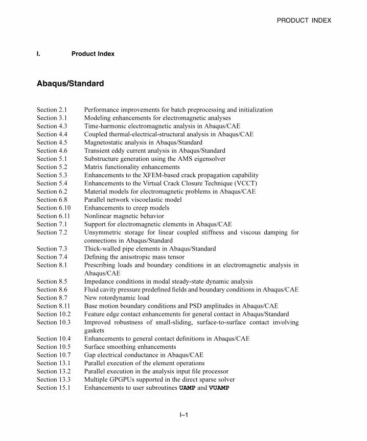
PRODUCT INDEX
I. Product Index
Abaqus/Standard
Section 2.1 Performance improvements for batch preprocessing and initialization
Section 3.1 Modeling enhancements for electromagnetic analyses
Section 4.3 Time-harmonic electromagnetic analysis in Abaqus/CAE
Section 4.4 Coupled thermal-electrical-structural analysis in Abaqus/CAE
Section 4.5 Magnetostatic analysis in Abaqus/Standard
Section 4.6 Transient eddy current analysis in Abaqus/Standard
Section 5.1 Substructure generation using the AMS eigensolver
Section 5.2 Matrix functionality enhancements
Section 5.3 Enhancements to the XFEM-based crack propagation capability
Section 5.4 Enhancements to the Virtual Crack Closure Technique (VCCT)
Section 6.2 Material models for electromagnetic problems in Abaqus/CAE
Section 6.8 Parallel network viscoelastic model
Section 6.10 Enhancements to creep models
Section 6.11 Nonlinear magnetic behavior
Section 7.1 Support for electromagnetic elements in Abaqus/CAE
Section 7.2 Unsymmetric storage for linear coupled stiffness and viscous damping for
connections in Abaqus/Standard
Section 7.3 Thick-walled pipe elements in Abaqus/Standard
Section 7.4 Defining the anisotropic mass tensor
Section 8.1 Prescribing loads and boundary conditions in an electromagnetic analysis in
Abaqus/CAE
Section 8.5 Impedance conditions in modal steady-state dynamic analysis
Section 8.6 Fluid cavity pressure predefined fields and boundary conditions in Abaqus/CAE
Section 8.7 New rotordynamic load
Section 8.11 Base motion boundary conditions and PSD amplitudes in Abaqus/CAE
Section 10.2 Feature edge contact enhancements for general contact in Abaqus/Standard
Section 10.3 Improved robustness of small-sliding, surface-to-surface contact involving
gaskets
Section 10.4 Enhancements to general contact definitions in Abaqus/CAE
Section 10.5 Surface smoothing enhancements
Section 10.7 Gap electrical conductance in Abaqus/CAE
Section 13.1 Parallel execution of the element operations
Section 13.2 Parallel execution in the analysis input file processor
Section 13.3 Multiple GPGPUs supported in the direct sparse solver
Section 15.1 Enhancements to user subroutines UAMP and VUAMP
I–1
Abaqus ID:
Printed on:
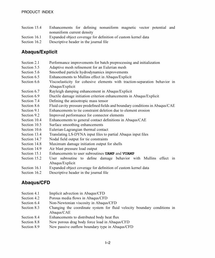
PRODUCT INDEX
Section 15.4 Enhancements for defining nonuniform magnetic vector potential and
nonuniform current density
Section 16.1 Expanded object coverage for definition of custom kernel data
Section 16.2 Descriptive header in the journal file
Abaqus/Explicit
Section 2.1 Performance improvements for batch preprocessing and initialization
Section 5.5 Adaptive mesh refinement for an Eulerian mesh
Section 5.6 Smoothed particle hydrodynamics improvements
Section 6.5 Enhancements to Mullins effect in Abaqus/Explicit
Section 6.6 Viscoelasticity for cohesive elements with traction-separation behavior in
Abaqus/Explicit
Section 6.7 Rayleigh damping enhancement in Abaqus/Explicit
Section 6.9 Ductile damage initiation criterion enhancements in Abaqus/Explicit
Section 7.4 Defining the anisotropic mass tensor
Section 8.6 Fluid cavity pressure predefined fields and boundary conditions in Abaqus/CAE
Section 9.1 Enhancements to tie constraint deletion due to element erosion
Section 9.2 Improved performance for connector elements
Section 10.4 Enhancements to general contact definitions in Abaqus/CAE
Section 10.5 Surface smoothing enhancements
Section 10.6 Eulerian-Lagrangian thermal contact
Section 13.4 Translating LS-DYNA input files to partial Abaqus input files
Section 14.7 Nodal field output for tie constraints
Section 14.8 Maximum damage initiation output for shells
Section 14.9 Air blast pressure load output
Section 15.1 Enhancements to user subroutines UAMP and VUAMP
Section 15.2 User subroutine to define damage behavior with Mullins effect in
Abaqus/Explicit
Section 16.1 Expanded object coverage for definition of custom kernel data
Section 16.2 Descriptive header in the journal file
Abaqus/CFD
Section 4.1 Implicit advection in Abaqus/CFD
Section 4.2 Porous media flows in Abaqus/CFD
Section 6.4 Non-Newtonian viscosity in Abaqus/CFD
Section 8.3 Changing the coordinate system for fluid velocity boundary conditions in
Abaqus/CAE
Section 8.4 Enhancements to distributed body heat flux
Section 8.8 New porous drag body force load in Abaqus/CFD
Section 8.9 New passive outflow boundary type in Abaqus/CFD
I–2
Abaqus ID:
Printed on:
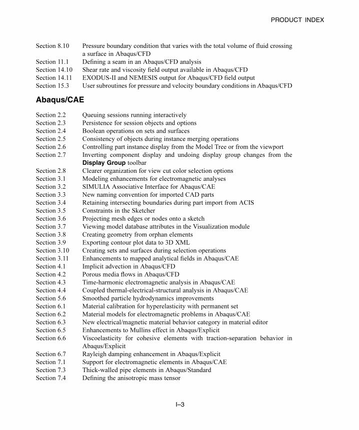
PRODUCT INDEX
Section 8.10 Pressure boundary condition that varies with the total volume of fluid crossing
a surface in Abaqus/CFD
Section 11.1 Defining a seam in an Abaqus/CFD analysis
Section 14.10 Shear rate and viscosity field output available in Abaqus/CFD
Section 14.11 EXODUS-II and NEMESIS output for Abaqus/CFD field output
Section 15.3 User subroutines for pressure and velocity boundary conditions in Abaqus/CFD
Abaqus/CAE
Section 2.2 Queuing sessions running interactively
Section 2.3 Persistence for session objects and options
Section 2.4 Boolean operations on sets and surfaces
Section 2.5 Consistency of objects during instance merging operations
Section 2.6 Controlling part instance display from the Model Tree or from the viewport
Section 2.7 Inverting component display and undoing display group changes from the
Display Group toolbar
Section 2.8 Clearer organization for view cut color selection options
Section 3.1 Modeling enhancements for electromagnetic analyses
Section 3.2 SIMULIA Associative Interface for Abaqus/CAE
Section 3.3 New naming convention for imported CAD parts
Section 3.4 Retaining intersecting boundaries during part import from ACIS
Section 3.5 Constraints in the Sketcher
Section 3.6 Projecting mesh edges or nodes onto a sketch
Section 3.7 Viewing model database attributes in the Visualization module
Section 3.8 Creating geometry from orphan elements
Section 3.9 Exporting contour plot data to 3D XML
Section 3.10 Creating sets and surfaces during selection operations
Section 3.11 Enhancements to mapped analytical fields in Abaqus/CAE
Section 4.1 Implicit advection in Abaqus/CFD
Section 4.2 Porous media flows in Abaqus/CFD
Section 4.3 Time-harmonic electromagnetic analysis in Abaqus/CAE
Section 4.4 Coupled thermal-electrical-structural analysis in Abaqus/CAE
Section 5.6 Smoothed particle hydrodynamics improvements
Section 6.1 Material calibration for hyperelasticity with permanent set
Section 6.2 Material models for electromagnetic problems in Abaqus/CAE
Section 6.3 New electrical/magnetic material behavior category in material editor
Section 6.5 Enhancements to Mullins effect in Abaqus/Explicit
Section 6.6 Viscoelasticity for cohesive elements with traction-separation behavior in
Abaqus/Explicit
Section 6.7 Rayleigh damping enhancement in Abaqus/Explicit
Section 7.1 Support for electromagnetic elements in Abaqus/CAE
Section 7.3 Thick-walled pipe elements in Abaqus/Standard
Section 7.4 Defining the anisotropic mass tensor
I–3
Abaqus ID:
Printed on:
PRODUCT INDEX
Section 8.1 Prescribing loads and boundary conditions in an electromagnetic analysis in
Abaqus/CAE
Section 8.2 New category choices for loads and boundary conditions in Abaqus/CAE
Section 8.3 Changing the coordinate system for fluid velocity boundary conditions in
Abaqus/CAE
Section 8.4 Enhancements to distributed body heat flux
Section 8.6 Fluid cavity pressure predefined fields and boundary conditions in Abaqus/CAE
Section 8.8 New porous drag body force load in Abaqus/CFD
Section 8.11 Base motion boundary conditions and PSD amplitudes in Abaqus/CAE
Section 8.12 Total flux distribution option for surface heat flux in Abaqus/CAE
Section 8.13 Defining connector loads and boundary conditions using assembled fasteners
and template models
Section 10.1 Surface fluid cavities and fluid exchanges in Abaqus/CAE
Section 10.4 Enhancements to general contact definitions in Abaqus/CAE
Section 10.5 Surface smoothing enhancements
Section 10.6 Eulerian-Lagrangian thermal contact
Section 10.7 Gap electrical conductance in Abaqus/CAE
Section 11.1 Defining a seam in an Abaqus/CFD analysis
Section 12.1 Local controls for tetrahedral meshing
Section 12.2 Combining orphan and native mesh features in a model
Section 12.3 Persistent display of seeds
Section 12.4 Enhanced node editing functionality
Section 12.5 Dragging nodes
Section 12.6 Improved display for selection of mesh parts
Section 12.7 Node and element numbering in flattened input files
Section 12.8 Adding a boundary layer to a tetrahedral mesh
Section 12.9 Mesh retention during feature additions and modifications
Section 14.1 Requesting field output on exterior nodes and elements in Abaqus/CAE
Section 14.2 Displaying multiple slices of view cut data
Section 14.3 Enhancements to free body display
Section 14.4 Editing free body cuts
Section 14.5 Selecting elements by topology in the Visualization module
Section 14.6 Enhancement to material orientation plot display
Section 14.7 Nodal field output for tie constraints
Section 14.8 Maximum damage initiation output for shells
Section 14.9 Air blast pressure load output
Section 14.12 Reading X–Y data from history output based on the step time
Section 14.13 Filtering selections for results output
Section 16.1 Expanded object coverage for definition of custom kernel data
Section 16.2 Descriptive header in the journal file
Section 16.3 Abaqus PDE improvements
Section 16.4 Skipping the last command during session recovery
I–4
Abaqus ID:
Printed on:
PRODUCT INDEX
Section 16.5 Faster tab completion
Section 16.6 Selected errors now classified as an AbaqusExceptionType
Section 16.7 Better control over writing messages to the journal file
Section 16.8 Reformatting commands in Python files with proper indentation
Section 16.9 Improved message handling and reporting of plug-ins
Section 16.10 Stop button for scripts
Abaqus/Viewer
Section 2.2 Queuing sessions running interactively
Section 3.7 Viewing model database attributes in the Visualization module
Abaqus/AMS
Section 5.1 Substructure generation using the AMS eigensolver
I–5
Abaqus ID:
Printed on:

About SIMULIASIMULIA is the Dassault Systèmes brand that delivers a scalable portfolio of Realistic Simulation solutions including the Abaqus product suite for Unified Finite Element Analysis; multiphysics solutions for insight into challenging engineering problems; and lifecycle management solutions for managing simulation data, processes, and intellectual property. By building on established technology, respected quality, and superior customer service, SIMULIA makes realistic simulation an integral business practice that improves product performance, reduces physical prototypes, and drives innovation. Headquartered in Providence, RI, USA, with R&D centers in Providence and in Vélizy, France, SIMULIA provides sales, services, and support through a global network of regional offices and distributors. For more information, visit www.simulia.com.
About Dassault SystèmesAs a world leader in 3D and Product Lifecycle Management (PLM) solutions, Dassault Systèmes brings value to more than 100,000 customers in 80 countries. A pioneer in the 3D software market since 1981, Dassault Systèmes develops and markets PLM application software and services that support industrial processes and provide a 3D vision of the entire lifecycle of products from conception to maintenance to recycling. The Dassault Systèmes portfolio consists of CATIA for designing the virtual product, SolidWorks for 3D mechanical design, DELMIA for virtual production, SIMULIA for virtual testing, ENOVIA for global collaborative lifecycle management, and 3DVIA for online 3D lifelike experiences. Dassault Systèmes’ shares are listed on Euronext Paris (#13065, DSY.PA), and Dassault Systèmes’ ADRs may be traded on the US Over-The-Counter (OTC) market (DASTY). For more information, visit www.3ds.com.
ww
w.3
ds.c
om
Aba
qus,
the
3DS
logo
, SIM
ULI
A, C
ATI
A, S
olid
Wor
ks, D
ELM
IA, E
NO
VIA
, 3D
VIA
, and
Uni
fied
FEA
are
trad
emar
ks o
r reg
iste
red
trad
emar
ks o
f D
assa
ult S
ystè
mes
or i
ts
subs
idia
ries
in th
e U
S an
d/or
oth
er c
ount
ries.
Oth
er c
ompa
ny, p
rodu
ct, a
nd s
ervi
ce n
ames
may
be
trad
emar
ks o
r ser
vice
mar
ks o
f the
ir re
spec
tive
owne
rs. ©
Das
saul
t Sys
tèm
es, 2
012