about the asian development bank erd working paper …econ.tu.ac.th/archan/rangsun/ec 460/ec 460...
TRANSCRIPT
Economics and REsEaRch dEpaRtmEnt
Printed in the Philippines
sectoral Engines of Growthin developing asia:stylized Factsand implications
Jesus Felipe, Miguel León-Ledesma, Matteo Lanzafame, and Gemma Estrada
November 2007
about the paper
Jesus Felipe, Miguel León-Ledesma, Matteo Lanzafame, and Gemma Estrada analyze the role that the different sectors of the economy have played as engines of growth in developing Asia. Both industry and services have propelled growth in the region. Likewise, technological spillovers, especially from Japan, have also played an important role as a source of growth.
Asian Development Bank6 ADB Avenue, Mandaluyong City1550 Metro Manila, Philippineswww.adb.org/economicsISSN: 1655-5252Publication Stock No.
about the asian development Bank
ADB aims to improve the welfare of the people in the Asia and Pacific region, particularly the nearly 1.9 billion who live on less than $2 a day. Despite many success stories, the region remains home to two thirds of the world’s poor. ADB is a multilateral development finance institution owned by 67 members, 48 from the region and 19 from other parts of the globe. ADB’s vision is a region free of poverty. Its mission is to help its developing member countries reduce poverty and improve their quality of life.
ADB’s main instruments for helping its developing member countries are policy dialogue, loans, equity investments, guarantees, grants, and technical assistance. ADB’s annual lending volume is typically about $6 billion, with technical assistance usually totaling about $180 million a year.
ADB’s headquarters is in Manila. It has 26 offices around the world and more than 2,000 employees from over 50 countries.
ERD WoRking PaPER SERiES no. 107

ERD Working Paper No. 107
Sectoral engineS of growth in Developing aSia: StylizeD factS anD implicationS
JeSuS felipe, miguel león-leDeSma,
matteo lanzafame, anD gemma eStraDa
november 2007
Jesus Felipe is Principal Economist in the Central and West Asia Department, Asian Development Bank; Miguel León-Ledesma is Senior Lecturer, Department of Economics, in the University of Kent (Canterbury, U.K.); Matteo Lanzafame is a graduate student in the University of Kent (Canterbury, U.K.); and Gemma Estrada is Economics Officer in the Macroeconomics and Finance Research Division, Asian Development Bank. This paper represents the views of the authors and does not represent those of the institutions or countries they represent.

Asian Development Bank6 ADB Avenue, Mandaluyong City1550 Metro Manila, Philippineswww.adb.org/economics
©2007 by Asian Development BankNovember 2007ISSN 1655-5252
The views expressed in this paperare those of the author(s) and do notnecessarily reflect the views or policiesof the Asian Development Bank.
FoREWoRD
The ERD Working Paper Series is a forum for ongoing and recently completed research and policy studies undertaken in the Asian Development Bank or on its behalf. The Series is a quick-disseminating, informal publication meant to stimulate discussion and elicit feedback. Papers published under this Series could subsequently be revised for publication as articles in professional journals or chapters in books.

CoNtENts
Abstract vii
I. INTRODUCTION 1
II. STRUCTURA�� TRANS�ORMATION IN DE�E��OPIN�� ASIAII. STRUCTURA�� TRANS�ORMATION IN DE�E��OPIN�� ASIA 2
III. STRUCTURA�� C�AN��E, INDUSTRIA��I�ATION, AND �A��DOR�S ��AWSIII. STRUCTURA�� C�AN��E, INDUSTRIA��I�ATION, AND �A��DOR�S ��AWS 7
A. �aldor�s ��awsA. �aldor�s ��aws 8
I�. AN E�AMINATION O� �A��DOR�S ��AWS 1I�. AN E�AMINATION O� �A��DOR�S ��AWS 11
A. �aldor�s �irst ��aw 11 B. �aldor�s Second ��aw 13 C. �aldor�s Third ��aw 15
�. PRODUCTION STRUCTURE SIMI��ARITIES, TEC�NO��O���� DI��USION,�. PRODUCTION STRUCTURE SIMI��ARITIES, TEC�NO��O���� DI��USION, AND CATC� UP 19
�I. CONC��USIONS 2�I. CONC��USIONS 22
RE�ERENCES 3RE�ERENCES 31

AbstRACt
This paper provides an analysis of developing Asia�s growth experience from the point of view of its structural transformation during the last three decades. The most salient feature of this transformation has been the significant decrease in the share of agriculture and the parallel increase in the share of services. The analysis uses �aldor�s framework to discuss whether industry plays the role of engine of growth in developing Asia. The empirical results show first, that both industry and services play such a role; and second, there is evidence of endogenous, growth-induced technological progress. ��ikewise, the technology gap approach supports the view that technological spillovers have fostered growth in developing Asia.

I. INtRoDUCtIoN
Except for those countries well endowed with natural resources such as oil, growth is always linked to the structural transformation of the economy. Indeed, the growth experience of the developed economies since the 19th century reveals that growth was associated to changes in the structure of the economy. More recently, the experience of the successful Asian economies (Republic of �orea [henceforth �orea]; Malaysia; Taipei,China etc.) also shows that high growth has been associated with deep changes in the structure of these economies. Moreover, many economists see the development of a modern industrial sector as the key for propelling structural transformation.
Structural transformation is reflected in changes in output and employment compositions. An economy that grows as a result of transformation generates new activities characterized by higher productivity and increasing returns to scale. The transition across different patterns of production and specialization also involves upgrading to higher value-added activities within each sector through the introduction of new products and processes. These changes entail far-reaching transformations in terms of, among other things, economic geography and skill content of output. It is the countries that can sustain multiple transitions across different stages of their structural transformation that grow successfully.
As Rodrik (2006) reminds us, development economists of the “old” school understood the key role that structural transformation plays in the course of development. Among these, it was probably Nicholas �aldor (1966 and 1967) who provided the most thorough explanation of why industry plays the role of “engine of growth.” Indeed, the so-called “�aldor�s ��aws” provide a solid starting point for sector analyses of growth and structural change.
The purpose of this paper is to analyze developing Asia�s growth experience in the context of structural transformation. ��rowth and structural transformation are interrelated, since countries do not grow by simply reproducing themselves on a larger scale. ��enerally (unless all sectors of the economy grow at identical rates), countries become different as they grow, not only in terms of what they produce, but also in terms of how they do it (i.e., by using different inputs, including methods of production).
Specifically, we attempt to answer the following questions: (i) What has been the extent of structural change in developing Asia during the last three decades? (ii) What is the contribution of the different sectors to the growth performance of the Asian economies? (iii) What is the contribution of structural change to productivity growth and catching up?
The rest of the paper is structured as follows. Section II documents the extent of structural transformation in developing Asia. Section III provides a brief summary of the literature on �aldor�s laws. Section I� discusses the empirical evidence provided by the laws. Section � complements the analysis of growth and structural transformation in Asia through �aldor�s laws with an analysis of the importance of structure and technology diffusion. Section �I summarizes the main findings.
� November 2007
Sectoral eNgiNeS of growth iN DevelopiNg aSia: StylizeD factS aND implicatioNSJeSuS felipe, miguel leóN-leDeSma, matteo laNzafame, aND gemma eStraDa
II. stRUCtURAL tRANsFoRMAtIoN IN DEVELoPING AsIA
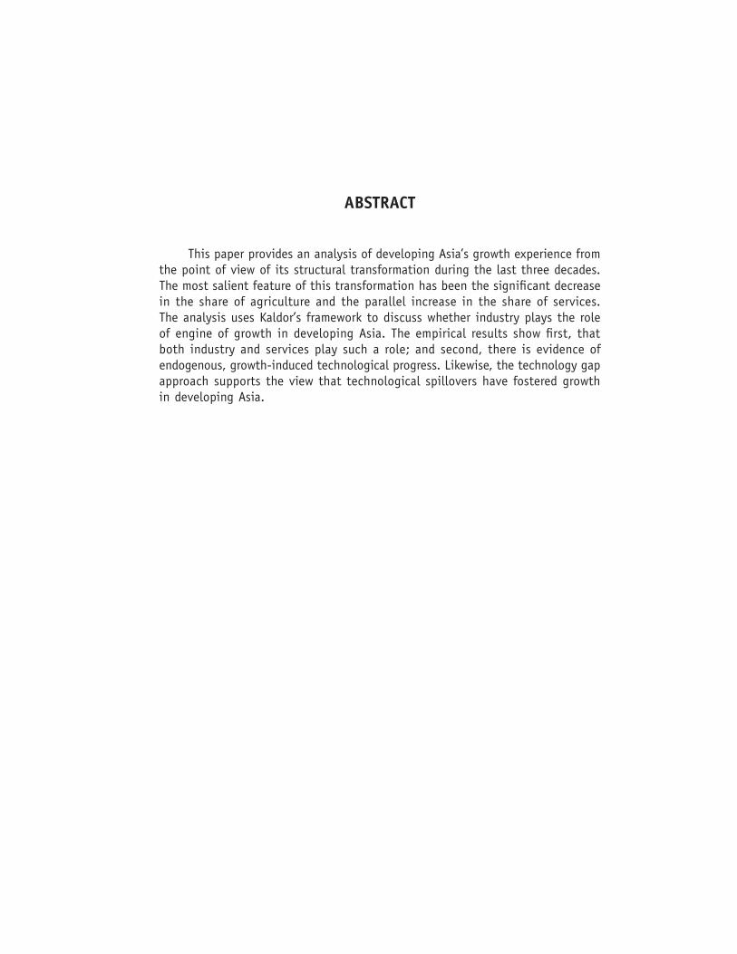
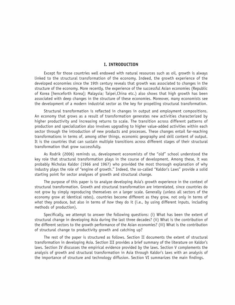
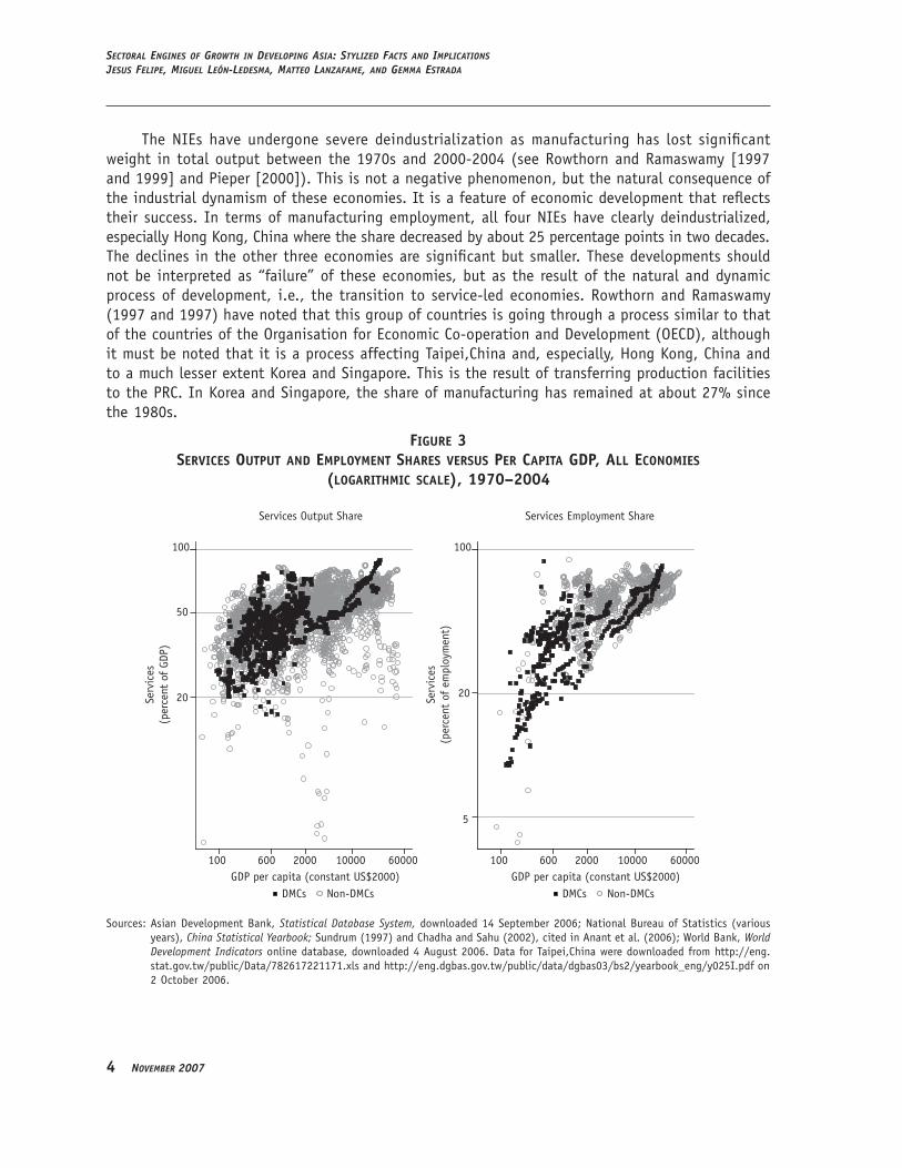
During the last three decades, most countries in developing Asia have undergone massive structural change, in particular in terms of changes in both output and employment sectoral shares. �igures 1, 2, and 3 show scatterplots of the output and employment shares of agriculture, industry, and services vis-à-vis income per capita, pooling data since 1970 for the whole world. �igure 1 shows that the shares of agricultural output and employment decline as countries become richer. �igure 2 shows that as countries� income per capita increases, so do the shares of output and employment in industry, although there seems to be a point beyond which these two shares start declining. �igure 2 also shows a wide dispersion in these shares for a given income per capita. �inally, the shares of output and employment in services clearly increase with increase with income per capita, a pattern referred to as logistic pattern. It is based on Engle�s law (demand explanation) and on the differential productivity growth rates across sectors (supply explanation).
figure 1agricultural output anD employment ShareS verSuS per capita gDp, all economieS
(logarithmic Scale), 1970–2004
Agricultural Output Share Agricultural Employment Share
100
50
20
5
100
50
20
5
Agric
ultu
re(p
erce
nt o
f GD
P)
Agric
ultu
re(p
erce
nt o
f em
ploy
men
t)
GDP per capita, constant US$2000 (in log scale)Developing Asia Rest of the world
GDP per capita, constant US$2000 (in log scale)Developing Asia Rest of the world
100 600 2000 10000 60000 100 600 2000 10000 60000
Sources: Asian Development Bank, Statistical Database System, downloaded 14 September 2006; National Bureau of Statistics (various years), China Statistical Yearbook; Sundrum (1997) and Chadha and Sahu (2002), cited in Anant et al. (2006); World Bank, World Development Indicators online database, downloaded 4 August 2006. Data for Taipei,China were downloaded from http://eng.stat.gov.tw/public/Data/782617221171.xls and http://eng.dgbas.gov.tw/public/data/dgbas03/bs2/yearbook_eng/y025I.pdf on 2 October 2006.
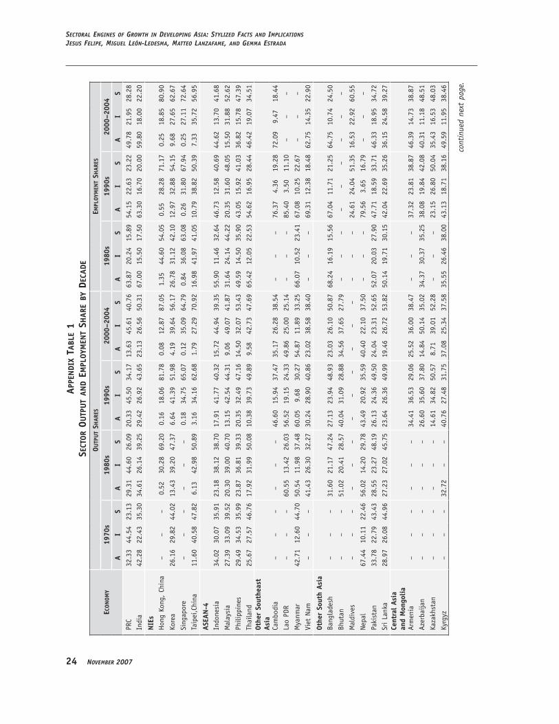
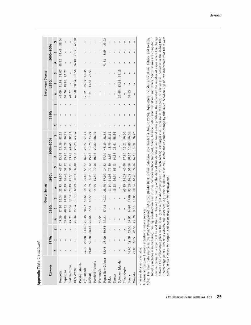
Appendix Tables 1, 2, and 3 show output and employment shares of the three sectors of the economy as well as of the manufacturing subsector by decade for developing Asia. The share of agricultural output in total output has declined significantly in all regions during the last 30
SectioN iiStructural traNSformatioN iN DevelopiNg aSia
erD workiNg paper SerieS No. 107 �
years. Especially significant are the declines that occurred in the People�s Republic of China (PRC) and India. Parallel to this decline, there has been an increase in the share of services also in all regions. The share of industry has increased significantly in some parts of developing Asia (e.g., ASEAN-4,1 Other Southeast Asia, Other South Asia); remained the same in the PRC; and increased by a small margin in India.
The share of employment in agriculture has also declined across the region, except in Central and West Asia (although in 2000–2004, agriculture was still the largest employer in developing Asia in 12 out of 23 countries for which data was available). This is the result of the convulsion that the region underwent after the collapse of the Soviet Union. �owever, the decline in agricultural employment has occurred at a much slower pace than that in output.
As in the case of the output share, there has been a generalized increase in the share of employment in services in all regions. Employment in industry has increased significantly in the ASEAN-4 countries (except the Philippines) and by a small margin in India; it has not changed in the PRC; and has suffered a decline in the newly industrialized economies or NIEs (especially �ong �ong, China) and across most of Central and West Asia.
figure 2inDuStry output anD employment ShareS verSuS per capita gDp, all economieS
(logarithmic Scale), 1970–2004
Industrial Output Share Industrial Employment Share
Indu
stry
(per
cent
of
GDP)
GDP per capita, constant US$2000 (in log scale)Developing Asia Rest of the world
GDP per capita, constant US$2000 (in log scale)Developing Asia Rest of the world
100
50
20
100
50
20
Indu
stry
(per
cent
of
empl
oym
ent)
100 600 2000 10000 60000 100 600 2000 10000 60000
Sources: Asian Development Bank, Statistical Database System, downloaded 14 September 2006; National Bureau of Statistics (various years), China Statistical Yearbook; Sundrum (1997) and Chadha and Sahu (2002), cited in Anant et al. (2006); World Bank, World Development Indicators online database, downloaded 4 August 2006. Data for Taipei,China were downloaded from http://eng.stat.gov.tw/public/Data/782617221171.xls and http://eng.dgbas.gov.tw/public/data/dgbas03/bs2/yearbook_eng/y025I.pdf on 2 October 2006.
1 The ASEAN-4 economies are Indonesia, Malaysia, Philippines, and Thailand.
� November 2007
Sectoral eNgiNeS of growth iN DevelopiNg aSia: StylizeD factS aND implicatioNSJeSuS felipe, miguel leóN-leDeSma, matteo laNzafame, aND gemma eStraDa
The NIEs have undergone severe deindustrialization as manufacturing has lost significant weight in total output between the 1970s and 2000-2004 (see Rowthorn and Ramaswamy [1997 and 1999] and Pieper [2000]). This is not a negative phenomenon, but the natural consequence of the industrial dynamism of these economies. It is a feature of economic development that reflects their success. In terms of manufacturing employment, all four NIEs have clearly deindustrialized, especially �ong �ong, China where the share decreased by about 25 percentage points in two decades. The declines in the other three economies are significant but smaller. These developments should not be interpreted as “failure” of these economies, but as the result of the natural and dynamic process of development, i.e., the transition to service-led economies. Rowthorn and Ramaswamy (1997 and 1997) have noted that this group of countries is going through a process similar to that of the countries of the Organisation for Economic Co-operation and Development (OECD), although it must be noted that it is a process affecting Taipei,China and, especially, �ong �ong, China and to a much lesser extent �orea and Singapore. This is the result of transferring production facilities to the PRC. In �orea and Singapore, the share of manufacturing has remained at about 27% since the 1980s.
figure 3ServiceS output anD employment ShareS verSuS per capita gDp, all economieS
(logarithmic Scale), 1970–2004
Services Output Share Services Employment Share
GDP per capita (constant US$2000)DMCs Non-DMCs
GDP per capita (constant US$2000)DMCs Non-DMCs
100 600 2000 10000 60000 100 600 2000 10000 60000
100
50
20
100
20
5
Serv
ices
(per
cent
of
GDP)
Serv
ices
(per
cent
of
empl
oym
ent)
Sources: Asian Development Bank, Statistical Database System, downloaded 14 September 2006; National Bureau of Statistics (various years), China Statistical Yearbook; Sundrum (1997) and Chadha and Sahu (2002), cited in Anant et al. (2006); World Bank, World Development Indicators online database, downloaded 4 August 2006. Data for Taipei,China were downloaded from http://eng.stat.gov.tw/public/Data/782617221171.xls and http://eng.dgbas.gov.tw/public/data/dgbas03/bs2/yearbook_eng/y025I.pdf on 2 October 2006.
SectioN iiStructural traNSformatioN iN DevelopiNg aSia
erD workiNg paper SerieS No. 107 �
The ASEAN-4 economies and other Southeast Asia have increased their manufacturing shares significantly, both in terms of output and employment. The exception is the Philippines, which had the highest manufacturing output share among the ASEAN-4 in the 1970s, but by 2000–2004 the share had decreased by about 3 percentage points and was the lowest in the group.
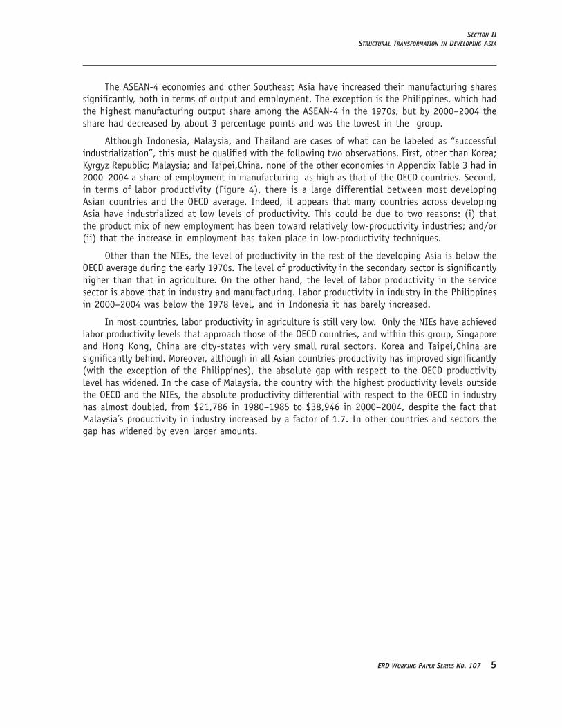
Although Indonesia, Malaysia, and Thailand are cases of what can be labeled as “successful industrialization”, this must be qualified with the following two observations. �irst, other than �orea; �yrgyz Republic; Malaysia; and Taipei,China, none of the other economies in Appendix Table 3 had in 2000–2004 a share of employment in manufacturing as high as that of the OECD countries. Second, in terms of labor productivity (�igure 4), there is a large differential between most developing Asian countries and the OECD average. Indeed, it appears that many countries across developing Asia have industrialized at low levels of productivity. This could be due to two reasons: (i) that the product mix of new employment has been toward relatively low-productivity industries; and/or (ii) that the increase in employment has taken place in low-productivity techniques.
Other than the NIEs, the level of productivity in the rest of the developing Asia is below the OECD average during the early 1970s. The level of productivity in the secondary sector is significantly higher than that in agriculture. On the other hand, the level of labor productivity in the service sector is above that in industry and manufacturing. ��abor productivity in industry in the Philippines in 2000–2004 was below the 1978 level, and in Indonesia it has barely increased.
In most countries, labor productivity in agriculture is still very low. Only the NIEs have achieved labor productivity levels that approach those of the OECD countries, and within this group, Singapore and �ong �ong, China are city-states with very small rural sectors. �orea and Taipei,China are significantly behind. Moreover, although in all Asian countries productivity has improved significantly (with the exception of the Philippines), the absolute gap with respect to the OECD productivity level has widened. In the case of Malaysia, the country with the highest productivity levels outside the OECD and the NIEs, the absolute productivity differential with respect to the OECD in industry has almost doubled, from $21,786 in 1980–1985 to $38,946 in 2000–2004, despite the fact that Malaysia�s productivity in industry increased by a factor of 1.7. In other countries and sectors the gap has widened by even larger amounts.
� November 2007
Sectoral eNgiNeS of growth iN DevelopiNg aSia: StylizeD factS aND implicatioNSJeSuS felipe, miguel leóN-leDeSma, matteo laNzafame, aND gemma eStraDa
figure 4total labor proDuctivity, logarithmic Scale (conStant 2000 uS DollarS)
100000
10000
1000
100
100000
10000
1000
100
100000
10000
1000
100
OECD
PRC
India
1970–75 76–79 80–85 86–89 90–95 96–99 2000–04
Singapore
OECD
Taipei,ChinaHongkong, China
1970–75 76–79 80–85 86–89 90–95 96–99 2000–04
100000
10000
1000
Rep. of Korea
OECD versus PRC and India
OECD versus ASEAN-4 OECD versus Other Asean Developing Countries
OECD versus NIEs
1970–75 76–79 80–85 86–89 90–95 96–99 2000–04 1970–75 76–79 80–85 86–89 90–95 96–99 2000–04
Indonesia
OECD
Philippines
Malaysia
Thailand Azerbaijan
OECD
PakistanKyrgyz Rep.
Viet Nam
Note: The 1980–1985, 1986–1989, 1990–1995, and 2000–2004 data for India refer only to 1983, 1988, 1994, and 2000 figures, respectively. Similarly, the 2000–2004 data for PRC, Indonesia, �yrgyz Republic, and Pakistan refer only to 2000–2002; the 1986–1989 data for Indonesia only to 1989; the 1976–1979 data for the Philippines only to 1978; and the 1970–1975 figure for Pakistan only to 1973–1975.
SectioN iiiStructural chaNge, iNDuStrializatioN, aND kalDor’S lawS
erD workiNg paper SerieS No. 107 7
III. stRUCtURAL CHANGE, INDUstRIALIZAtIoN, AND KALDoR’s LAWs
The evidence presented so far clearly points toward a rapid process of structural transformation in developing Asia. In order to understand the potential role of this transformation, it is important to view these changes in light of the development theory literature. The role attributed to manufacturing in the process of take-off and catching-up is usually a key element of sectoral studies of growth. It is no surprise, hence, that economists and policymakers worry about swings affecting the manufacturing sector.
It is in this context that the �aldorian sectoral growth facts or laws (�aldor 1966 and 1967) become very relevant as an approach to the issue of how structural change has affected growth in developing Asia, and what is the role that the different sectors have played. The �aldorian facts bring together the notion of “engine of growth” sectors, “economies of scale”, and “sectoral shifts” in a simple yet informative way. This framework recognizes that some sectors may play a more important role in pulling the rest of the economy and generating productivity gains through economies of scale.
�aldor�s laws allow us to address empirically the following questions: (i) Is manufacturing still an engine of growth in Asia? (ii) Can services play a role as engine of growth? (iii) What are the most dynamic sectors in Asian countries? (iv) Can we expect continued growth in Asia, given the recent sectoral developments? It should be noted that we view �aldor�s laws more as a series of stylized facts and historical regularities rather than a theory of economic development. These facts are compatible with a diverse range of theories of growth. What is important is that these correlations are presented at the sectoral level and, hence, are helpful in analyzing and comparing patterns of economic growth and the role of structure. In this sense, our objective is “estimating”, rather than “testing”, these laws, following the distinction put forward by ��eamer and ��evinsohn (1995).
The role attributed to manufacturing in the process of take-off and subsequent catch-up is usually a key element of sector studies of growth. It is no surprise, therefore, that economists and policymakers worry about swings in manufacturing. Though economies like Australia, Canada, New �ealand, the Scandinavian countries, and others relied heavily on the primary sector for their development, they all experienced periods of strong industrial growth and diversification as essential components of their sustained economic growth. Rodrik (2006) has argued that sustained growth requires a dynamic industrial base. One can, therefore, speak of the “logic of industrialization” (Nixson 1990, 313) and understand why many developing countries have adopted strategies toward rapid industrialization, often starting with industries that use relatively simple technologies and that have the potential to be labor-intensive and thus absorb labor, such as textiles, clothing, and shoes. The experience of the industrial economies shows that establishing a broad and robust domestic industrial base holds the key to successful development, and the reason that industrialization matters lies in the potential for strong productivity and income growth of the sector. This potential is associated also with a strong investment drive in the sector, rapidly rising productivity, and a growing share of the sector in total output and employment. The presence of scale economies associated with the secondary sector, gains from specialization and learning, as well as favorable global market conditions imply that the creation of leading industrial subsectors, along with related technological and social capabilities, remains a key policy challenge. Today, there is wide variety across countries in terms of resource endowments, pace of capital accumulation, and policy choices. This implies that there is ample room for diversity in industrial development.
� November 2007
Sectoral eNgiNeS of growth iN DevelopiNg aSia: StylizeD factS aND implicatioNSJeSuS felipe, miguel leóN-leDeSma, matteo laNzafame, aND gemma eStraDa
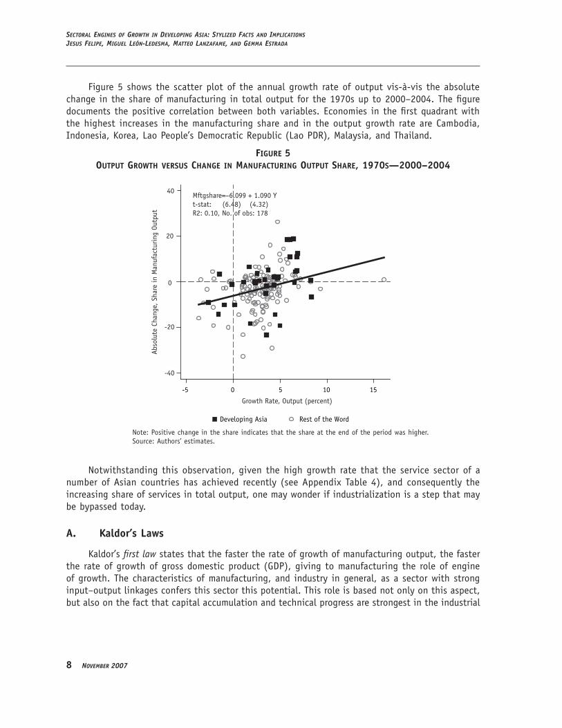
�igure 5 shows the scatter plot of the annual growth rate of output vis-à-vis the absolute change in the share of manufacturing in total output for the 1970s up to 2000–2004. The figure documents the positive correlation between both variables. Economies in the first quadrant with the highest increases in the manufacturing share and in the output growth rate are Cambodia, Indonesia, �orea, ��ao People�s Democratic Republic (��ao PDR), Malaysia, and Thailand.
figure 5output growth verSuS change in manufacturing output Share, 1970S—2000–2004
40
20
-20
-40
0
Abso
lute
Cha
nge,
Sha
re in
Man
ufac
turi
ng O
utpu
t
Growth Rate, Output (percent)
Developing Asia Rest of the Word
-5 0 5 10 15
Mftgshare=−6.099 + 1.090 Yt-stat: (6.48) (4.32)R2: 0.10, No. of obs: 178
Note: Positive change in the share indicates that the share at the end of the period was higher.Source: Authors� estimates.
Notwithstanding this observation, given the high growth rate that the service sector of a number of Asian countries has achieved recently (see Appendix Table 4), and consequently the increasing share of services in total output, one may wonder if industrialization is a step that may be bypassed today.
A. Kaldor’s Laws
�aldor�s first law states that the faster the rate of growth of manufacturing output, the faster the rate of growth of gross domestic product (��DP), giving to manufacturing the role of engine of growth. The characteristics of manufacturing, and industry in general, as a sector with strong input–output linkages confers this sector this potential. This role is based not only on this aspect, but also on the fact that capital accumulation and technical progress are strongest in the industrial
SectioN iiiStructural chaNge, iNDuStrializatioN, aND kalDor’S lawS
erD workiNg paper SerieS No. 107 �
sector, having important spillover effects on the rest of the economy. This means that the stronger the rate of growth of manufacturing, the stronger the rate of growth of the rest of the economy. �aldor viewed the high growth rates characteristics of middle-income countries as an attribute of the process of industrialization.
In his seminal work and for empirical purposes, �aldor specified the laws as relationships between growth rates because he estimated a cross section of countries with data at two points in time. �aldor�s first law, i.e., that manufacturing acts as the engine of growth, can be examined through a regression of nonmanufacturing output growth ( Ynm ) on manufacturing output growth ( Ym ), was therefore specified as
ˆ ˆY a a Ynm m= +1 2 (1)
where a2 indicates the strength and size of the impact (elasticity) of the manufacturing sector�s growth on the rest of the economy. This coefficient, therefore, can be viewed as the main indicator of the “engine of growth” role of this sector. Similar regressions are estimated for agriculture, industry, and services to assess their capacity as engines of growth.
�aldor�s second law states that there is a strong positive relationship between the growth of manufacturing production and the growth of manufacturing productivity. This law is also known as �erdoorn�s ��aw and has been interpreted as evidence in support of the existence of increasing returns in the manufacturing sector (see, for example, McCombie et al. 2002). The expansion of output leads to a process of macro-dynamic increasing returns that derive in productivity gains. This can also be interpreted from the point of view of employment creation: sectors subject to scale economies have lower employment elasticities with respect to output, as productivity grows as a by-product of output expansion.2 As productivity growth equals output growth minus employment growth, regressing productivity on total growth could induce spurious correlation. �or this reason, �erdoorn�s law, i.e., the induced productivity growth effect linked to increasing returns, is specified as a regression of manufacturing employment growth ( em ) on manufacturing output growth ( Ym
). Algebraically,
ˆ ˆe b b Ym m= +1 2 (2)
�aldor�s hypothesis is that output expansion induces a less than proportional employment expansion that leads to productivity gains. The coefficient b2 , the elasticity of employment with respect to output, is an indicator of the degree of increasing returns. The closer to 1, the smaller the induced productivity growth and returns to scale. Traditionally, estimates of the coefficient for manufacturing are close to 0.5. With a few assumptions about the capital–output ratio, a 0.5 coefficient implies increasing returns in a standard production function (see Ros 2000, 130–3). The interpretation of this coefficient is that each additional percentage point in the growth of output is associated with a 0.5% increase in employment and a 0.5% increase in the growth of productivity. As in the case of the first law, similar regressions are estimated for agriculture, industry, and services.
As mentioned earlier, rather than interpreting the �aldorian model of growth as a theoretical explanation of the “ultimate” causes of growth, these hypotheses are formulated empirically through 2 It is also the result of a second mechanism, wherein employment growth in industry tends to increase the rate of growth
of productivity in other sectors. This is the consequence of diminishing returns to labor in other sectors, absorption of surplus labor from these sectors, as well as of faster increase in the flow of goods into consumption.
10 November 2007
Sectoral eNgiNeS of growth iN DevelopiNg aSia: StylizeD factS aND implicatioNSJeSuS felipe, miguel leóN-leDeSma, matteo laNzafame, aND gemma eStraDa
regressions (1) and (2) and interpreted as stylized facts that can shed light on the questions posed above. Thus, these two hypotheses provide a set of growth facts at the sectoral level that can be used in conjunction with several theoretical interpretations to formulate a well-informed analysis of the prospective growth performance of the Asian countries. �aldor�s laws, when viewed as a set of empirical regularities, appear to be consistent with many growth models that do not rely on diminishing returns to capital. The division of labor and ideas-driven growth models of Romer (1986 and 1990), ��ucas (1988), and Aghion and �owitt (1992) are all consistent with �aldor�s second law, although they are set up in economies without an explicit sectoral structure.
�aldor�s third law states that when manufacturing grows, the rest of the sectors (not subject to increasing returns) will transfer labor to manufacturing, raising the overall productivity of the economy. Dynamic sectors absorb workers from the stagnant ones in which the level and growth of labor productivity is very low. This raises the overall productivity level of the economy and its rate of growth. The key mechanisms that explain how structural change affects productivity growth through compositional effects were developed by Baumol et al. (1985 and 1989). According to their view, backward economies with a large pool of employment in low-productivity activities (normally agriculture) experience a bonus from structural change. This “structural bonus” arises as a result of the transfer of labor from low- to high-productivity activities. This will automatically increase the productivity level of the economy. This happens even if this transfer of resources constitutes mainly a shift from agriculture to services. �owever, as the logistic pattern of structural change drives resources toward services, and given that productivity growth in this sector is usually slower than in industry, countries experience a “structural burden.” This “burden” means that the process of structural change has a negative impact on productivity growth. In the limit, as most of the labor force has moved into the services activities, economies experience “asymptotic stagnancy” as productivity growth is mostly determined by the services sector.3
The relationship between �aldor�s third law and Baumol�s asymptotic stagnancy theory is evident. The importance of a sector depends not only on its role in generating scale economies, but also on how it absorbs resources from other sectors, leading to “structural bonus” and “structural burden” effects. Although a sector with low productivity growth can absorb resources from agriculture leading to increased productivity levels, this source of economic growth is asymptotically exhausted. In the transition process, �aldor�s third law will be an important source of growth but, in the limit, induced productivity growth is the key to generating growth (see, for example, �agerberg 2000, Timmer and Szirmai 2000).
3 This description of how resource transfers in the process of structural change affect growth is very useful to analyzeThis description of how resource transfers in the process of structural change affect growth is very useful to analyze compositional effects. �owever, three aspects have to be noted. �irst, the concept of asymptotic stagnancy is a relative one. That is, growth is driven by activities whose productivity grows at a relatively slower rate than industry, but productivity growth may still be high in absolute terms. Second, it is assumed that services are necessarily a slow productivity growth sector. �owever, the distinction between stagnant and dynamic sectors has become blurred in recent decades by technological advances that have provoked very important changes in the organization and productivity of many services activities. �inally, although it is almost tautological that employment shifts toward the more labor-intensive activities, the model does not consider that growth in the different sectors is interdependent. That is, the expansion of some activities, especially those with increasing returns, can have an important impact on productivity in other activities. New growth theory has emphasized how the expansion of markets leads to increased division of labor and intermediate products leading to more sophisticated production processes that can be enjoyed by all the sectors in the economy. Similarly, some activities with more traditional input–output linkages can act as engines of growth through backward and forward effects on other sectors. Innovation and knowledge accumulation are but another source of sectoral spillovers that link together the developments of different sectors independently of their relative size in the economy.
SectioN ivaN examiNatioN of kalDor’S lawS
erD workiNg paper SerieS No. 107 11
IV. AN EXAMINAtIoN oF KALDoR’s LAWs
Regressions of �aldor�s first two laws were conducted using a panel of 17 developing Asian countries for 1980–2004. The panel is unbalanced as data for some countries for some years are missing at the beginning of the sample. The lack of consistent time-series data on employment for Bangladesh, India, and ��ao PDR prevented us from including these countries in the regression of the second law. The exploitation of both cross-sectional and time series data allows us to include all relevant information that would be thrown away in pure cross-sectional average estimates. The models are estimated in log levels using cointegration techniques, as the traditional growth rates specification may be simply capturing business cycle correlations that are not the focus of the investigation.
This panel of time-series allows us to address other potentially relevant problems. The first one is the bias that might be associated from the endogeneity of the regressors. Although our interest is in the stylized fact stemming from the reduced form, and not in a structural interpretation, endogeneity may induce biases in the estimated coefficients. �or this reason we use a fully modified ordinary least squares (�MO��S) panel cointegration estimator, as advocated by Pedroni (2000). This is an estimator for heterogeneous panels that allows us to obtain a panel estimate of the coefficient as well as country-specific coefficients. A homogeneous cointegration vector is estimated, but fixed effects and short-run dynamics are allowed to be unit-specific.
The second problem that may arise is that there may be a high degree of correlation between the different variables across countries. World shocks affecting variables such as the terms of trade may induce cross-sectional correlation and also correlation between the regressed variables, unrelated to the �aldorian hypotheses that are the focus of the analysis. �or this reason, we also provide estimates of the panel cointegration coefficients including heterogeneous (country-specific) unobserved components estimated by obtaining principal components.4 This estimate allows for a high degree of heterogeneity as well, but assumes common slope coefficients. We refer to these estimates as UC (unobserved component) elasticities.
A. Kaldor’s First Law
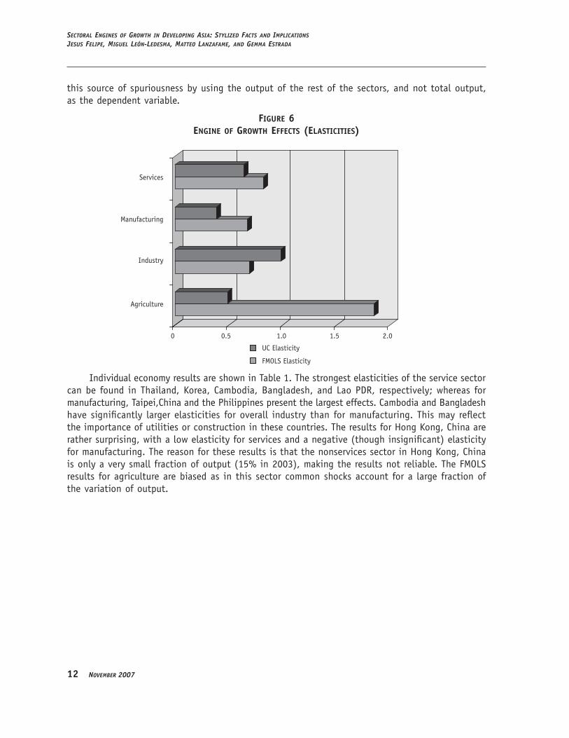
Estimation results of the first law are summarized in �igure 6, which shows the estimated long-run elasticities of output of the rest of the economy with respect to output in each one of the sectors.5 The sector with the largest engine of growth elasticity, after controlling for common shocks, is industry. This is followed by services and manufacturing. Agriculture appears to have a very large impact using the �MO��S estimate. The introduction of the unobserved component (UC elasticity) reduces the size of the elasticity significantly. This is because agricultural output is likely to be highly correlated across countries due to common shocks stemming from, for example, climate conditions and terms of trade shocks. The larger elasticity of industry relative to manufacturing reflects the fact that industrial activities such as electricity and other utilities have important forward and backward linkages with the rest of the economy.
These results also indicate that both industry and services have acted as the engines of growth in developing Asia during the period analyzed. It is important to note that services have a larger impact than manufacturing. This is not due to mere compositional effects, as we have avoided 4 See �orni et al. (2001). We included only the first principal component in the model.See �orni et al. (2001). We included only the first principal component in the model.ee �orni et al. (2001). We included only the first principal component in the model.5 Cointegration tests showed that all variables in this specification were cointegrated.
1� November 2007
Sectoral eNgiNeS of growth iN DevelopiNg aSia: StylizeD factS aND implicatioNSJeSuS felipe, miguel leóN-leDeSma, matteo laNzafame, aND gemma eStraDa
this source of spuriousness by using the output of the rest of the sectors, and not total output, as the dependent variable.
figure 6engine of growth effectS (elaSticitieS)
Services
Manufacturing
Industry
Agriculture
UC Elasticity
FMOLS Elasticity
0 0.5 1.0 1.5 2.0
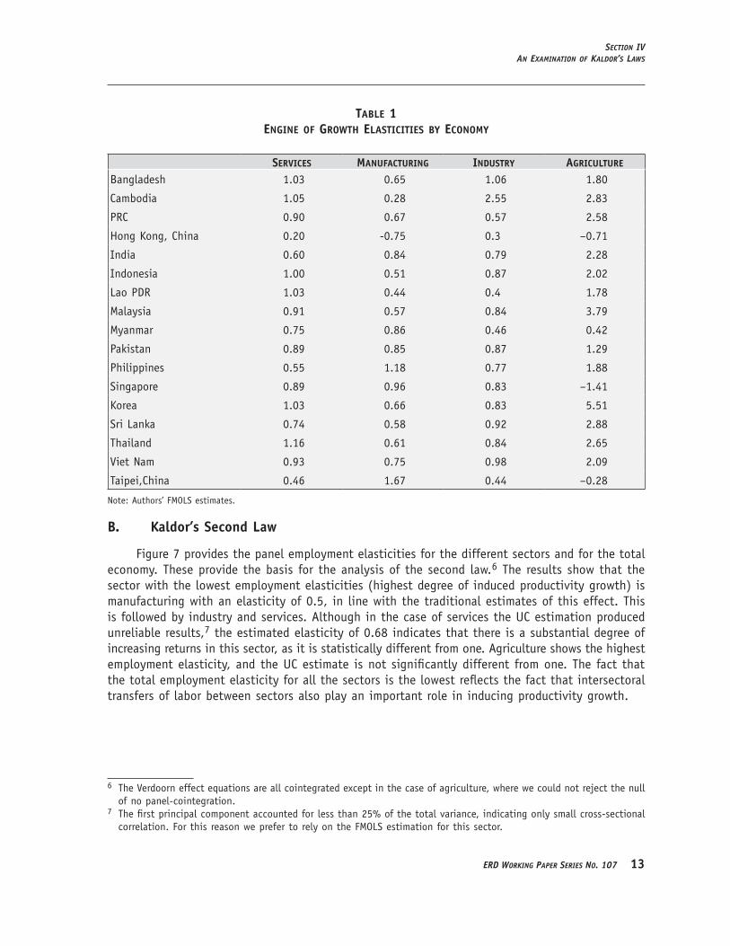
Individual economy results are shown in Table 1. The strongest elasticities of the service sector can be found in Thailand, �orea, Cambodia, Bangladesh, and ��ao PDR, respectively; whereas for manufacturing, Taipei,China and the Philippines present the largest effects. Cambodia and Bangladesh have significantly larger elasticities for overall industry than for manufacturing. This may reflect the importance of utilities or construction in these countries. The results for �ong �ong, China are rather surprising, with a low elasticity for services and a negative (though insignificant) elasticity for manufacturing. The reason for these results is that the nonservices sector in �ong �ong, China is only a very small fraction of output (15% in 2003), making the results not reliable. The �MO��S results for agriculture are biased as in this sector common shocks account for a large fraction of the variation of output.
SectioN ivaN examiNatioN of kalDor’S lawS
erD workiNg paper SerieS No. 107 1�
table 1engine of growth elaSticitieS by economy
ServiceS manufacturing inDuStry agriculture
Bangladesh 1.03 0.65 1.06 1.80
Cambodia 1.05 0.28 2.55 2.83
PRC 0.90 0.67 0.57 2.58
�ong �ong, China 0.20 -0.75 0.3 –0.71
India 0.60 0.84 0.79 2.28
Indonesia 1.00 0.51 0.87 2.02
��ao PDR 1.03 0.44 0.4 1.78
Malaysia 0.91 0.57 0.84 3.79
Myanmar 0.75 0.86 0.46 0.42
Pakistan 0.89 0.85 0.87 1.29
Philippines 0.55 1.18 0.77 1.88
Singapore 0.89 0.96 0.83 –1.41
�orea 1.03 0.66 0.83 5.51
Sri ��anka 0.74 0.58 0.92 2.88
Thailand 1.16 0.61 0.84 2.65
�iet Nam 0.93 0.75 0.98 2.09
Taipei,China 0.46 1.67 0.44 –0.28
Note: Authors� �MO��S estimates.
b. Kaldor’s second Law
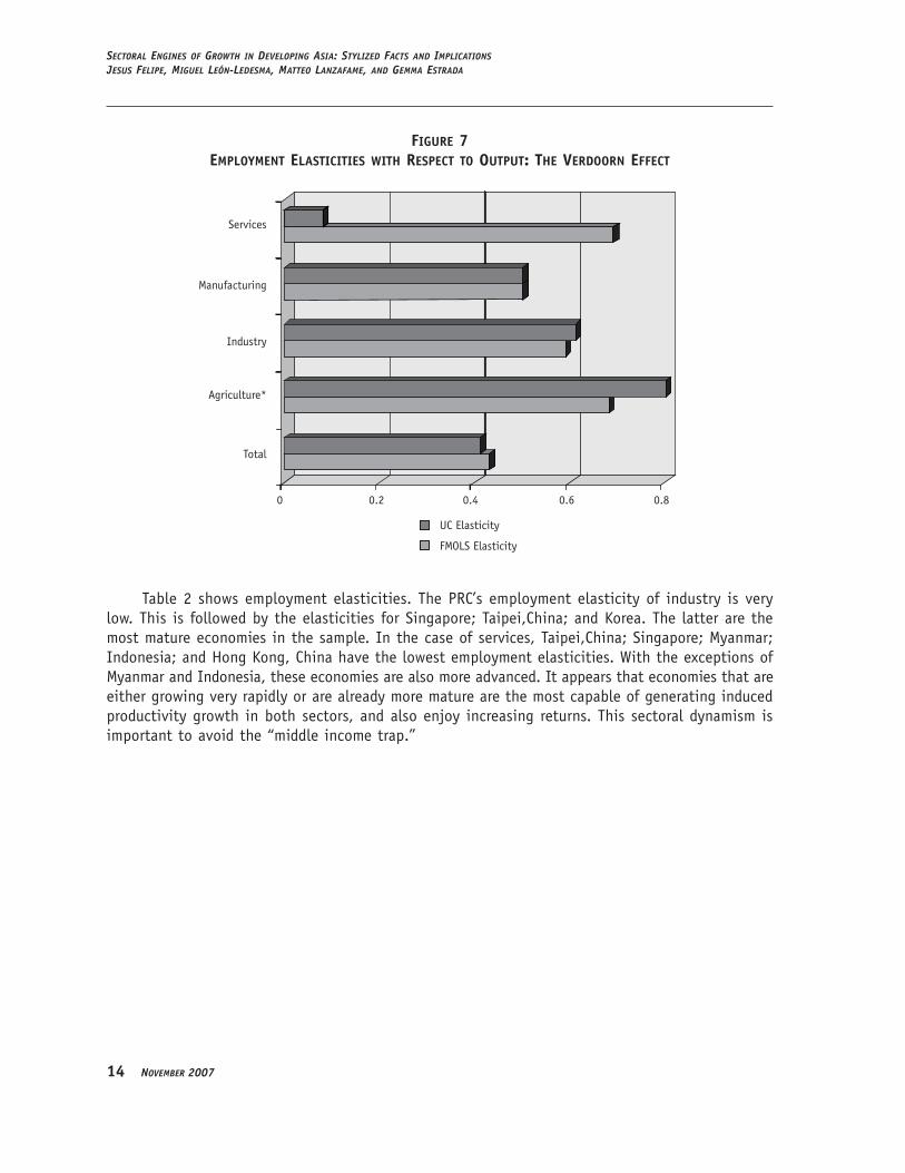
�igure 7 provides the panel employment elasticities for the different sectors and for the total economy. These provide the basis for the analysis of the second law.6 The results show that the sector with the lowest employment elasticities (highest degree of induced productivity growth) is manufacturing with an elasticity of 0.5, in line with the traditional estimates of this effect. This is followed by industry and services. Although in the case of services the UC estimation produced unreliable results,7 the estimated elasticity of 0.68 indicates that there is a substantial degree of increasing returns in this sector, as it is statistically different from one. Agriculture shows the highest employment elasticity, and the UC estimate is not significantly different from one. The fact that the total employment elasticity for all the sectors is the lowest reflects the fact that intersectoral transfers of labor between sectors also play an important role in inducing productivity growth.
6 The �erdoorn effect equations are all cointegrated except in the case of agriculture, where we could not reject the null of no panel-cointegration.
7 The first principal component accounted for less than 25% of the total variance, indicating only small cross-sectional correlation. �or this reason we prefer to rely on the �MO��S estimation for this sector.
1� November 2007
Sectoral eNgiNeS of growth iN DevelopiNg aSia: StylizeD factS aND implicatioNSJeSuS felipe, miguel leóN-leDeSma, matteo laNzafame, aND gemma eStraDa
figure 7employment elaSticitieS with reSpect to output: the verDoorn effect
Services
Manufacturing
Industry
Agriculture*
Total
UC Elasticity
FMOLS Elasticity
0 0.2 0.4 0.6 0.8
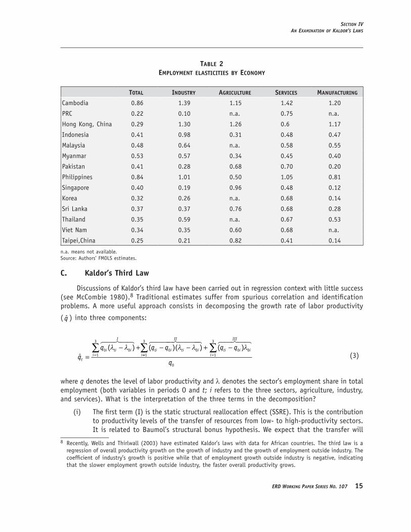
Table 2 shows employment elasticities. The PRC�s employment elasticity of industry is very low. This is followed by the elasticities for Singapore; Taipei,China; and �orea. The latter are the most mature economies in the sample. In the case of services, Taipei,China; Singapore; Myanmar; Indonesia; and �ong �ong, China have the lowest employment elasticities. With the exceptions of Myanmar and Indonesia, these economies are also more advanced. It appears that economies that are either growing very rapidly or are already more mature are the most capable of generating induced productivity growth in both sectors, and also enjoy increasing returns. This sectoral dynamism is important to avoid the “middle income trap.”
SectioN ivaN examiNatioN of kalDor’S lawS
erD workiNg paper SerieS No. 107 1�
table 2employment elaSticitieS by economy
total inDuStry agriculture ServiceS manufacturing
Cambodia 0.86 1.39 1.15 1.42 1.20
PRC 0.22 0.10 n.a. 0.75 n.a.
�ong �ong, China 0.29 1.30 1.26 0.6 1.17
Indonesia 0.41 0.98 0.31 0.48 0.47
Malaysia 0.48 0.64 n.a. 0.58 0.55
Myanmar 0.53 0.57 0.34 0.45 0.40
Pakistan 0.41 0.28 0.68 0.70 0.20
Philippines 0.84 1.01 0.50 1.05 0.81
Singapore 0.40 0.19 0.96 0.48 0.12
�orea 0.32 0.26 n.a. 0.68 0.14
Sri ��anka 0.37 0.37 0.76 0.68 0.28
Thailand 0.35 0.59 n.a. 0.67 0.53
�iet Nam 0.34 0.35 0.60 0.68 n.a.
Taipei,China 0.25 0.21 0.82 0.41 0.14
n.a. means not available. Source: Authors� �MO��S estimates.
C. Kaldor’s third Law
Discussions of �aldor�s third law have been carried out in regression context with little success (see McCombie 1980).8 Traditional estimates suffer from spurious correlation and identification problems. A more useful approach consists in decomposing the growth rate of labor productivity
( q ) into three components:
ˆ( ) ( )( )
qq q q
t
i ti i
I
iti i ti i
II
i=− + − −
=∑ 0 0
1
3
0 0λ λ λ λ
== =∑ ∑+ −
1
3
0 01
3
0
( )q q
q
ti i i
III
i
λ
(3)
where q denotes the level of labor productivity and λ denotes the sector�s employment share in total employment (both variables in periods O and t; i refers to the three sectors, agriculture, industry, and services). What is the interpretation of the three terms in the decomposition?
(i) The first term (I) is the static structural reallocation effect (SSRE). This is the contribution to productivity levels of the transfer of resources from low- to high-productivity sectors. It is related to Baumol�s structural bonus hypothesis. We expect that the transfer will
8 Recently, Wells and Thirlwall (2003) have estimated �aldor�s laws with data for African countries. The third law is a regression of overall productivity growth on the growth of industry and the growth of employment outside industry. The coefficient of industry�s growth is positive while that of employment growth outside industry is negative, indicating that the slower employment growth outside industry, the faster overall productivity grows.

1� November 2007
Sectoral eNgiNeS of growth iN DevelopiNg aSia: StylizeD factS aND implicatioNSJeSuS felipe, miguel leóN-leDeSma, matteo laNzafame, aND gemma eStraDa
increase the average level of productivity of the economy as employment shares shift from agriculture to services. This effect is calculated by shifting employment shares, keeping initial productivity levels of each sector constant.
(ii) The second term second term (II) is the dynamic structural reallocation effect (DSRE), and represents the contribution of the resource transfer to productivity growth. It is related to Baumol�s structural burden hypothesis as employment transfers toward services—a sector with (in general, though not always) lower productivity growth—reduce the overall productivity growth of the economy. The effect is calculated as the interaction between employment shifts and productivity growth.
(iii) The final term (III) is the within-sector productivity growth (WS). It is the contribution of productivity growth within each sector to overall productivity growth. This is the growth of productivity that is not explained by sectoral shifts. It is calculated by keeping employment shares constant and allowing productivity levels to change.
The importance of making the distinction between the static and dynamic structural reallocation effects is that it helps distinguish between the structural bonus and burden effects of employment reallocation. Countries with large agricultural sectors have a lot to gain from the bonus of surplus labor in low-productivity activities. �owever, if the growth of employment is predominantly in sectors with lower scope for productivity growth, there is a burden effect. If productivity growth in services is lower than in manufacturing, this imposes a “relative” burden (though not absolute). Note, however, that in �aldor�s interpretation, this reallocation is “induced” by growth of the leading sector. This hypothesis cannot be examined directly by shift-share analysis, but it is clear that it is the growing sectors that will draw resources from those contracting.
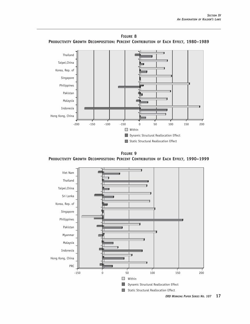
The contribution of sectoral shifts to productivity growth embedded in the third law is presented in �igures 8, 9, and 10. We have decomposed productivity growth into its three components for three different subperiods, 1980–1989, 1990–1999, and 2000–2004. The average contribution of each effect throughout 1980–2004 is approximately 33% for the static structural reallocation effect (SSRE), –14% for the dynamic structural reallocation effect (DSRE), and 81% for within-sector productivity growth effect (WS). �or 1980–1989, these percentages are 15.6%, –22%, and 106.5%, respectively. �or 1990–1999, they are 40%, –6% and 66%, respectively; whereas for the final period the figures are 44%, –13%, and 69%, respectively. This shows that the SSRE gained importance during the last 15 years. The figures, however, mask large differences across countries. Nevertheless, they point toward the WS effect as the main driver of overall productivity growth. Within-sector productivity growth is related to productivity gains stemming from scale economies and, importantly, technology absorption from frontier economies such as Europe, Japan, and United States (US).9 The impact of the SSRE is non-negligible, accounting for one third of productivity growth. This effect is mainly the result of the transfer of labor from agriculture into services. As expected, the DSRE is negative and related to the structural burden hypothesis.
9 Technology adoption can be thought of as a function of explicit research and development investment, human capital, foreign direct investment, and also structural composition of output in the sector.
SectioN ivaN examiNatioN of kalDor’S lawS
erD workiNg paper SerieS No. 107 17
figure 8proDuctivity growth DecompoSition: percent contribution of each effect, 1980–1989
Thailand
Taipei,China
Korea, Rep. of
Singapore
Philippines
Pakistan
Malaysia
Indonesia
Hong Kong, China
-200 -150 -100 -150 0 50 100 150 200
Within
Dynamic Structural Reallocation Effect
Static Structural Reallocation Effect
figure 9proDuctivity growth DecompoSition: percent contribution of each effect, 1990–1999
-150 0 50 100 150 200
Viet Nam
Thailand
Taipei,China
Sri Lanka
Korea, Rep. of
Singapore
Philippines
Pakistan
Myanmar
Malaysia
Indonesia
Hong Kong, China
PRC
Within
Dynamic Structural Reallocation Effect
Static Structural Reallocation Effect
1� November 2007
Sectoral eNgiNeS of growth iN DevelopiNg aSia: StylizeD factS aND implicatioNSJeSuS felipe, miguel leóN-leDeSma, matteo laNzafame, aND gemma eStraDa
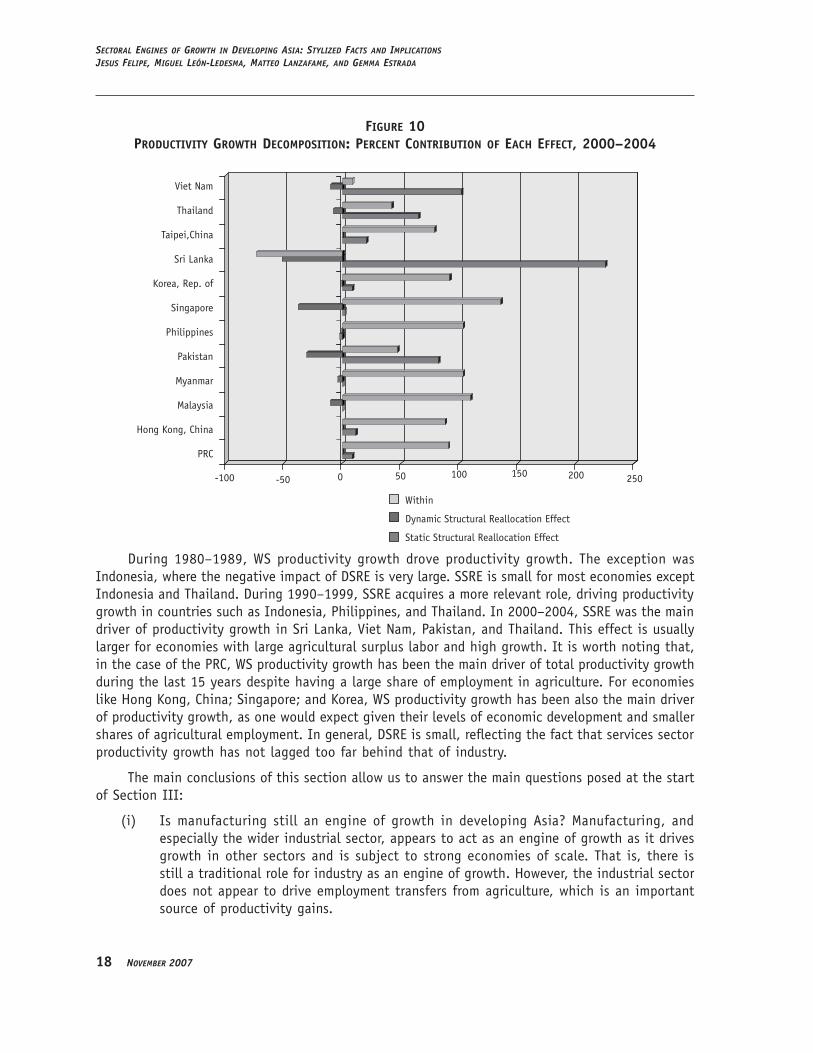
figure 10proDuctivity growth DecompoSition: percent contribution of each effect, 2000–2004
-50-100 0 50 100 150 200
Viet Nam
Thailand
Taipei,China
Sri Lanka
Korea, Rep. of
Singapore
Philippines
Pakistan
Myanmar
Malaysia
Hong Kong, China
PRC
250
Within
Dynamic Structural Reallocation Effect
Static Structural Reallocation Effect
During 1980–1989, WS productivity growth drove productivity growth. The exception was Indonesia, where the negative impact of DSRE is very large. SSRE is small for most economies except Indonesia and Thailand. During 1990–1999, SSRE acquires a more relevant role, driving productivity growth in countries such as Indonesia, Philippines, and Thailand. In 2000–2004, SSRE was the main driver of productivity growth in Sri ��anka, �iet Nam, Pakistan, and Thailand. This effect is usually larger for economies with large agricultural surplus labor and high growth. It is worth noting that, in the case of the PRC, WS productivity growth has been the main driver of total productivity growth during the last 15 years despite having a large share of employment in agriculture. �or economies like �ong �ong, China; Singapore; and �orea, WS productivity growth has been also the main driver of productivity growth, as one would expect given their levels of economic development and smaller shares of agricultural employment. In general, DSRE is small, reflecting the fact that services sector productivity growth has not lagged too far behind that of industry.
The main conclusions of this section allow us to answer the main questions posed at the start of Section III:
(i) Is manufacturing still an engine of growth in developing Asia? Manufacturing, and especially the wider industrial sector, appears to act as an engine of growth as it drives growth in other sectors and is subject to strong economies of scale. That is, there is still a traditional role for industry as an engine of growth. �owever, the industrial sector does not appear to drive employment transfers from agriculture, which is an important source of productivity gains.
SectioN vproDuctioN Structure SimilaritieS, techNology DiffuSioN, aND catch up
erD workiNg paper SerieS No. 107 1�
(ii) Can services play a role as engine of growth? The evidence shows that services have a strong and large impact on the growth of the other sectors. Indeed, this impact is larger than industry�s. Although to a lesser extent than in industry, services appear to have significant productivity growth-inducing effects through the exploitation of scale economies. Services also appear to be driving productivity gains through factor reallocation effects.
(iii) What are the most dynamic sectors in developing Asian countries? Although there are important differences across countries, both industry and services can be thought of as the dynamic sectors of Asian economies. The evidence points toward a key role for industry but, very importantly, services appear to have been able to play this dynamic role as well. The old distinction between industry and services as the dynamic and stagnant sectors of an economy, respectively, does not appear to hold true in the context of the Asian countries.
(iv) Can we expect continued growth in Asia, given the recent developments at the sector level? The scope for growth is still very large. This is because productivity growth is likely to continue in many Asian economies through two sources. �irst, factor reallocation toward services, especially for the middle-low income countries in the sample, is not likely to be exhausted as a source of growth in the short run. Second, WS productivity growth through catching-up and exploitation of scale economies is likely to continue being the main driver of productivity gains in the future.
Overall, this implies that there is significant evidence of endogenous, growth-induced technological progress in developing Asia.
V. PRoDUCtIoN stRUCtURE sIMILARItIEs, tECHNoLoGY DIFFUsIoN, AND CAtCH UP
In this section we address the third question posed in the introduction, namely, what is the contribution of structural change to productivity growth and catching up? While regression analysis of the first two �aldorian hypotheses for the Asian countries has provided significant evidence of endogenous, growth-induced technological progress, for countries lagging behind the technological frontier, endogenous technological progress will be partly dependent on the acquisition and mastering of more advanced production techniques from the leader countries, which in turn will be determined by such factors as national research and development, human capital, and trade openness.
�urthermore, if technology is (at least to a certain extent) sector-specific, its diffusion from the most advanced to the less advanced countries will be more intense and faster the higher the degree of structural (or sectoral) similarity between them. As a result, ceteris paribus, technological progress will be faster for a less advanced country, the more its production structure resembles that of the technological leader. This reasoning is in line with Abramovitz (1986 and 1993), who has argued that the extent to which developing economies can benefit from the superior technology developed in advanced countries depends on their “absorption capability.” The latter is itself a composite variable, determined by social as well as economic and structural factors, such as the degree of “technological congruence” with countries on the technological frontier.
�ere we propose a simple approach to measuring the significance of the extent to which the productivity growth performance of the Asian countries benefited from technological spillovers from the most advanced countries flowing via a “structural channel.”
�0 November 2007
Sectoral eNgiNeS of growth iN DevelopiNg aSia: StylizeD factS aND implicatioNSJeSuS felipe, miguel leóN-leDeSma, matteo laNzafame, aND gemma eStraDa
�irst, in the spirit of the technology gap approach to growth and convergence (��erschenkron 1962, Nelson and Wright 1992), we define a measure of the potential for technology transfer from the most advanced to the less advanced countries as given by the labor productivity ratio between
the two, i.e., GAP t
q tq ti
L
i
( )( )( )
=, where t denotes time, q tL( ) is the level of labor productivity in the
technologically most advanced country, and q ti ( ) its counterpart in the less advanced country i.
Second, we devise a measure of structural similarity making use of �rugman�s specialization index (or �-index) developed by Midelfart-�narvirk et al. (2000).10 At each point in time, the index is constructed as the sum over the k sectors of the absolute differences between the sectors� shares of value-added in country i and in the technological leader. Its value ranges between zero and two and increases with the degree of specialization, i.e., it is higher the more a country�s production structure differs from that of the technological leader. �or instance, a �-index value of 0.5 indicates that 25% of the country i’s production structure is out of line with that of the technologically most advanced country, in the sense that one quarter of its total output does not correspond to the average sectoral composition in the latter.11
This way, one can build a structurally weighted gap variable by first designing a measure of
structural weights as W tK t
iL
iL( ) = −( )
12
, where 0 1≤ ( ) ≤W tiL
, which increases with the degree of structural
similarity, i.e., as K tiL
( ) falls. The structurally weighted gap variable is SWGAP t W GAP ti iL i( ) ( ).= × This variable can then be introduced in a growth regression (see Temple 1999) to capture the idea that the impact of technology spillovers on the less advanced countries� growth performance will be dependent not only on the size of the technology gap but also on the degree of structural similarity between technological leaders and followers. We examine this hypothesis by making use of a simple reduced-form growth equation.
��iven the nature of the hypothesis under examination, finely sectorally disaggregated data are essential for estimation proposes. Taking this into account, we restrict our attention to manufacturing
and construct the structural weights W tiL
( ) using data for 28 sectors from the United Nations Industrial Development Organization.12 The remaining data are taken from the World Bank World Development Indicators (WDI) and the International ��abour Organisation (I��O).13
10 When applied to country-level bilateral comparisons it is constructed as: K t abs v t v tiL ik
Lk
k( ) ( ) - ( )= ∑ , where
v tx t
x tik i
k
ik
k
( )( )
( )≡
∑ and x tik( ) denotes country i�s value-added in sector k at time t and refers to the technological leader.
Instead of value-added, Midelfart-�narvirk et al. (2000) employed the gross value of output as a measure of activity level, on the grounds that this makes the results of the analysis less likely to be biased by the effects of structural shifts in outsourcing to other sectors. This option was precluded by data unavailability in our case.
11 The upper bound of the index equals two because, by construction, it takes into account both positive and negativeThe upper bound of the index equals two because, by construction, it takes into account both positive and negative deviations across sectors. Thus, when calculating the “implied-percentage deviation” the value in question must be halved: in the example, (0.5/2)%=25%.
12 The data are from the Industrial Statistics Database 2006 at the 3-digit level of ISIC Code (Revision 2) (UNIDO 2006).
13 The source of the manufacturing value added series for the US is the Department of Commerce, Bureau of Economic Analysis.
SectioN vproDuctioN Structure SimilaritieS, techNology DiffuSioN, aND catch up
erD workiNg paper SerieS No. 107 �1
To smooth out cyclical effects, structural weights W tiL
( ) were computed as 3-year moving averages of annual values. The regression was estimated by means of panel data techniques using an unbalanced panel of annual data over 1982–2002 for nine Asian economies, namely Bangladesh; PRC; �ong �ong, China; Indonesia; Malaysia; Singapore; �orea; Sri ��anka; and Taipei,China. The regression estimated is:
q GAP SWGAPit i i itj
j itj
jj
= + +==
∑∑α β θ1
2
1
2
(4)
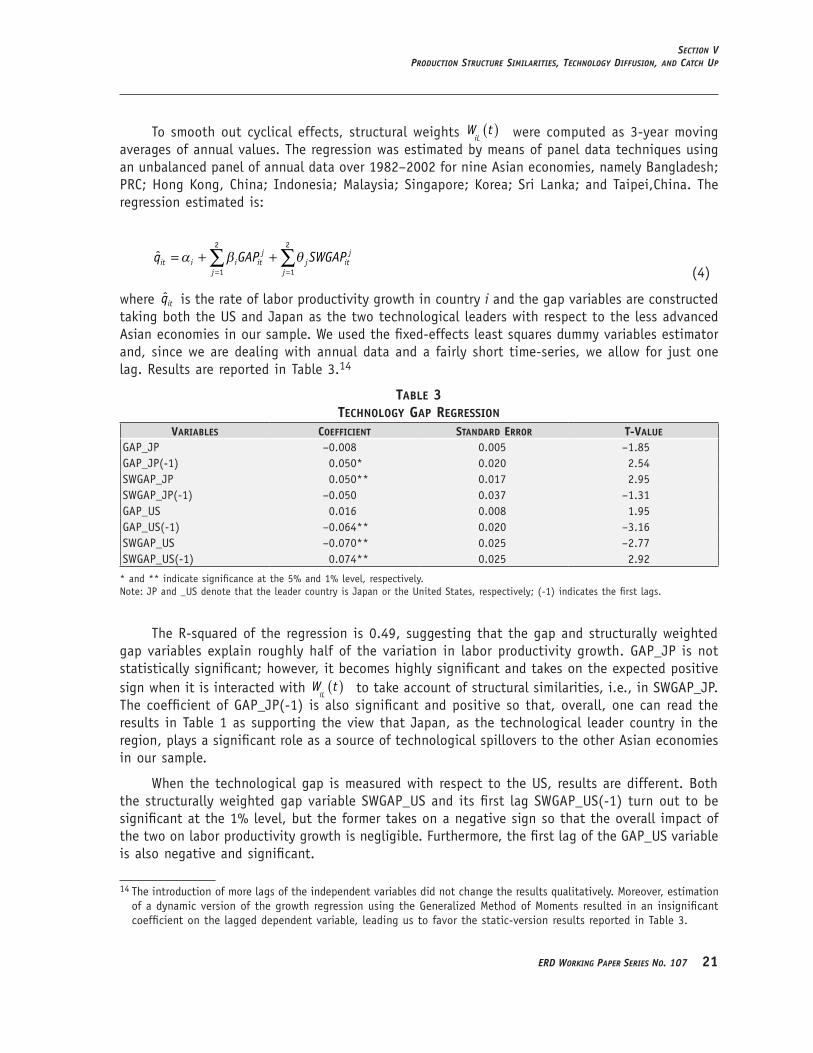
where qit is the rate of labor productivity growth in country i and the gap variables are constructed taking both the US and Japan as the two technological leaders with respect to the less advanced Asian economies in our sample. We used the fixed-effects least squares dummy variables estimator and, since we are dealing with annual data and a fairly short time-series, we allow for just one lag. Results are reported in Table 3.14
table 3technology gap regreSSion
variableS coefficient StanDarD error t-value
��AP_JP –0.008 0.005 –1.85��AP_JP(-1) 0.050* 0.020 2.54SW��AP_JP 0.050** 0.017 2.95SW��AP_JP(-1) –0.050 0.037 –1.31��AP_US 0.016 0.008 1.95��AP_US(-1) –0.064** 0.020 –3.16SW��AP_US –0.070** 0.025 –2.77SW��AP_US(-1) 0.074** 0.025 2.92
* and ** indicate significance at the 5% and 1% level, respectively.Note: JP and _US denote that the leader country is Japan or the United States, respectively; (-1) indicates the first lags.
The R-squared of the regression is 0.49, suggesting that the gap and structurally weighted gap variables explain roughly half of the variation in labor productivity growth. ��AP_JP is not statistically significant; however, it becomes highly significant and takes on the expected positive sign when it is interacted with W t
iL( ) to take account of structural similarities, i.e., in SW��AP_JP.
The coefficient of ��AP_JP(-1) is also significant and positive so that, overall, one can read the results in Table 1 as supporting the view that Japan, as the technological leader country in the region, plays a significant role as a source of technological spillovers to the other Asian economies in our sample.
When the technological gap is measured with respect to the US, results are different. Both the structurally weighted gap variable SW��AP_US and its first lag SW��AP_US(-1) turn out to be significant at the 1% level, but the former takes on a negative sign so that the overall impact of the two on labor productivity growth is negligible. �urthermore, the first lag of the ��AP_US variable is also negative and significant.
14 The introduction of more lags of the independent variables did not change the results qualitatively. Moreover, estimation of a dynamic version of the growth regression using the ��eneralized Method of Moments resulted in an insignificant coefficient on the lagged dependent variable, leading us to favor the static-version results reported in Table 3.
�� November 2007
Sectoral eNgiNeS of growth iN DevelopiNg aSia: StylizeD factS aND implicatioNSJeSuS felipe, miguel leóN-leDeSma, matteo laNzafame, aND gemma eStraDa
VI. CoNCLUsIoNs
The most salient feature of developing Asia�s transformation during the last three decades has been the significant decrease in the share of agriculture and the parallel increase in the share of services. Some parts of developing Asia have clearly industrialized in the sense that the shares of industry and manufacturing in total output have increased (e.g., Indonesia, Malaysia, Thailand). But many other countries in the region have not seen an increase in these shares. The richest economies in the region, the NIEs, are undergoing a deindustrialization process. This simply reflects their shift to high value-added services. �arious other countries in the region have had difficulties in industrializing. India and the Philippines are among the most significant examples, although for India, recent data seem to indicate that its manufacturing share has increased. Others (e.g., the Pacific economies) face industrialization as a very difficult process, since they have limited opportunities to start with. It is important to note that the patterns of structural transformation of output and employment are different, as the decline in agricultural employment is taking place at a much slower pace than that of output. This has led, in many countries across the region, to rather “asymmetric” output and employment structures. Indeed, one could say that much of the region looks like a service economy in terms of output, but an agricultural economy in terms of employment. An additional important feature of structural change in developing Asia is that, despite its rapid growth, the level of labor productivity in most of the region still lags far behind that of industrial countries. ��iven that investments were made in highly productive industry and services segments of the economy, this implies that there are still many other large segments of the economy with very low productivity. Structural transformation in developing Asia is taking place through a combination of modern and sophisticated industry and services with high and rising productivity levels, with many other backward ones (probably where a large part of the labor from agriculture is being transferred) that operate at very low productivity levels. �inally, the analysis of structural transformation from the point of view of technology and scale indicates that only a few countries in the region have undergone a significant upgrade.
Regressions of �aldor�s laws indicate that both industry and services appear to have acted as engines of growth in the Asian economies. The manufacturing sector is subject to strong increasing returns, although in services the degree of increasing returns is indeed non-negligible too. Although the share of industry and manufacturing is shrinking in total employment, this does not necessarily imply that their role as the most dynamic sectors has decreased. Induced productivity growth in manufacturing can indeed be seen as the reason for its decline as a share of output for countries that had previously industrialized. Notable exceptions are the PRC and India. In the former, industrial activity remains relatively very important and in the latter large-scale industrialization has not occurred. Services appear to have contributed largely to growth as they drag employment from the less productive agricultural sector. Although induced productivity growth in services is smaller than in industry, services appear to be a remarkably dynamic sector. Both factors together have contributed to the importance of services as an engine of growth. As the large reserves of employment in agriculture are exhausted, the contribution of services to productivity growth is likely to decrease as its productivity growth is lower than that of industry.
This will largely depend on the composition of services between dynamic and stagnant activities. �owever, there is no reason to believe that, in the medium run, growth will decline due to the increase in the share of services in total output. There are three main reasons for this:
erD workiNg paper SerieS No. 107 ��
(i) There is still a very large scope for structural change, especially in the less developed economies of Asia.
(ii) The role of the dynamic industrial sector remains very relevant for economies where industrialization occurred previously.
(iii) The scope of within-sector productivity growth is still very large. This is likely to be facilitated by structural change itself, which increases the capacity of Asian economies to absorb foreign technology. This catching-up process is likely to lead to important productivity gains in services.
�inally, the technology gap approach, as formalized in the framework used here, provides a simple way to analyze the impact of technology diffusion on the growth performance of the Asian countries. The results support the view that technological spillovers foster growth when Japan is taken as the technological leader, but is not the case when the leader-country is the US. Moreover, structural similarity seems to be playing a significant part in the process of technology diffusion both from Japan and the US, although the overall influence from the latter is fairly small.
SectioN vicoNcluSioNS
�� November 2007
Sectoral eNgiNeS of growth iN DevelopiNg aSia: StylizeD factS aND implicatioNSJeSuS felipe, miguel leóN-leDeSma, matteo laNzafame, aND gemma eStraDa
appe
nDi
x ta
ble
1Se
ctor
ou
tpu
t an
D em
ploy
men
t Sh
are
by D
ecaD
e
econ
omy
outp
ut
Shar
eSem
ploy
men
t Sh
areS
1�70
s1�
�0s
1��0
s�0
00–�
00�
1��0
s1�
�0s
�000
–�00
�A
Is
AI
sA
Is
AI
sA
Is
AI
sA
Is
PRC
32.3
3 44
.54
23.1
3 29
.31
44.6
0 26
.09
20.3
3 45
.50
34.1
7 13
.63
45.6
1 40
.76
63.8
7 20
.24
15.8
9 54
.15
22.6
3 23
.22
49.7
8 21
.95
28.2
8 In
dia
42.2
8 22
.43
35.3
0 34
.61
26.1
4 39
.25
29.4
2 26
.92
43.6
5 23
.13
26.5
6 50
.31
67.0
0 15
.50
17.5
0 63
.30
16.7
0 20
.00
59.8
0 18
.00
22.2
0
NIE
s
�on
g �o
ng,
Chin
a –
– –
0.52
30
.28
69.2
0 0.
16
18.0
6 81
.78
0.08
12
.87
87.0
5 1.
35
44.6
0 54
.05
0.55
28
.28
71.1
7 0.
25
18.8
5 80
.90
�ore
a26
.16
29.8
2 44
.02
13.4
3 39
.20
47.3
7 6.
64
41.3
9 51
.98
4.19
39
.64
56.1
7 26
.78
31.1
2 42
.10
12.9
7 32
.88
54.1
5 9.
68
27.6
5 62
.67
Sing
apor
e –
– –
– –
–0.
18
34.7
5 65
.07
0.12
35
.09
64.7
9 0.
84
36.0
8 63
.08
0.26
31
.80
67.9
4 0.
25
27.1
1 72
.64
Taip
ei,C
hina
11.6
0 40
.58
47.8
2 6.
13
42.9
8 50
.89
3.16
34
.16
62.6
8 1.
79
27.2
9 70
.92
16.9
8 41
.97
41.0
5 10
.79
38.8
2 50
.39
7.33
35
.72
56.9
5
AsEA
N-�
Indo
nesi
a34
.02
30.0
7 35
.91
23.1
8 38
.12
38.7
0 17
.91
41.7
7 40
.32
15.7
2 44
.94
39.3
5 55
.90
11.4
6 32
.64
46.7
3 12
.58
40.6
9 44
.62
13.7
0 41
.68
Mal
aysi
a27
.39
33.0
9 39
.52
20.3
0 39
.00
40.7
0 13
.15
42.5
4 44
.31
9.06
49
.07
41.8
7 31
.64
24.1
4 44
.22
20.3
5 31
.60
48.0
5 15
.50
31.8
8 52
.62
Phili
ppin
es29
.49
34.5
3 35
.99
23.8
7 36
.81
39.3
3 20
.35
32.4
9 47
.16
14.5
0 32
.07
53.4
3 49
.59
14.5
0 35
.90
43.0
5 15
.92
41.0
3 36
.82
15.7
8 47
.39
Thai
land
25.6
7 27
.57
46.7
6 17
.92
31.9
9 50
.08
10.3
8 39
.73
49.8
9 9.
58
42.7
3 47
.69
65.4
2 12
.05
22.5
3 54
.62
16.9
5 28
.44
46.4
2 19
.07
34.5
1 ot
her
sout
heas
t As
iaCa
mbo
dia
– –
– –
– –
46.6
0 15
.94
37.4
7 35
.17
26.2
8 38
.54
– –
–76
.37
4.36
19
.28
72.0
9 9.
47
18.4
4
��ao
PDR
– –
–60
.55
13.4
2 26
.03
56.5
2 19
.15
24.3
3 49
.86
25.0
0 25
.14
– –
–85
.40
3.50
11
.10
– –
–
Mya
nmar
42.7
1 12
.60
44.7
0 50
.54
11.9
8 37
.48
60.0
5 9.
68
30.2
7 54
.87
11.8
9 33
.25
66.0
7 10
.52
23.4
1 67
.08
10.2
5 22
.67
– –
–
�iet
Nam
– –
–41
.43
26.3
0 32
.27
30.2
4 28
.90
40.8
6 23
.02
38.5
8 38
.40
– –
–69
.31
12.3
8 18
.48
62.7
5 14
.35
22.9
0
othe
r so
uth
Asia
Bang
lade
sh –
– –
31.6
0 21
.17
47.2
4 27
.13
23.9
4 48
.93
23.0
3 26
.10
50.8
7 68
.24
16.1
9 15
.56
67.0
4 11
.71
21.2
5 64
.75
10.7
4 24
.50
Bhut
an –
– –
51.0
2 20
.41
28.5
7 40
.04
31.0
9 28
.88
34.5
6 37
.65
27.7
9 –
– –
– –
– –
– –
Mal
dive
s –
– –
– –
– –
– –
– –
– –
– –
24.6
1 24
.04
51.3
5 16
.53
22.9
2 60
.55
Nepa
l67
.44
10.1
1 22
.46
56.0
2 14
.20
29.7
8 43
.49
20.9
2 35
.59
40.4
0 22
.10
37.5
0 –
– –
79.5
6 3.
65
16.7
9 –
– –
Paki
stan
33.7
8 22
.79
43.4
3 28
.55
23.2
7 48
.19
26.1
3 24
.36
49.5
0 24
.04
23.3
1 52
.65
52.0
7 20
.03
27.9
0 47
.71
18.5
9 33
.71
46.3
3 18
.95
34.7
2
Sri
��ank
a28
.97
26.0
8 44
.96
27.2
3 27
.02
45.7
5 23
.64
26.3
6 49
.99
19.4
6 26
.72
53.8
2 50
.14
19.7
1 30
.15
42.0
4 22
.69
35.2
6 36
.15
24.5
8 39
.27
Cent
ral
Asia
an
d M
ongo
lia
Arm
enia
– –
– –
– –
34.4
1 36
.53
29.0
6 25
.52
36.0
0 38
.47
– –
–37
.32
23.8
1 38
.87
46.3
9 14
.73
38.8
7
Azer
baija
n –
– –
– –
–26
.60
35.6
0 37
.80
14.8
4 50
.14
35.0
2 34
.37
30.3
7 35
.25
38.0
8 19
.84
42.0
8 40
.31
11.1
8 48
.51
�aza
khst
an –
– –
– –
–14
.61
34.8
2 50
.57
8.71
39
.01
52.2
8 –
– –
23.1
5 26
.80
50.0
4 35
.43
16.5
3 48
.03
�yrg
yz –
– –
32.7
2 –
–40
.76
27.4
8 31
.75
37.0
8 25
.34
37.5
8 35
.55
26.4
6 38
.00
43.1
3 18
.71
38.1
6 49
.59
11.9
5 38
.46
cont
inue
d ne
xt p
age.
erD workiNg paper SerieS No. 107 ��
econ
omy
outp
ut
Shar
eSem
ploy
men
t Sh
areS
1�70
s1�
�0s
1��0
s�0
00–�
00�
1��0
s1�
�0s
�000
–�00
�A
Is
AI
sA
Is
AI
sA
Is
AI
sA
Is
Mon
golia
––
–17
.36
27.3
0 55
.34
33.7
3 24
.90
41.3
7 23
.12
24.3
6 52
.52
––
–47
.09
21.8
4 31
.07
45.9
2 14
.43
39.6
4
Tajik
ista
n–
––
32.0
6 40
.11
27.8
3 31
.19
36.4
3 32
.37
25.9
0 37
.29
36.8
1 –
––
57.7
6 19
.96
24.7
7 –
––
Turk
men
ista
n–
––
27.7
7 37
.06
35.1
7 23
.49
45.5
0 31
.01
23.2
3 44
.45
32.3
3 –
––
44.7
7 –
––
––
Uzb
ekis
tan
––
–29
.34
35.5
4 35
.13
32.7
9 30
.11
37.1
0 33
.37
23.2
9 43
.34
––
–42
.50
20.9
4 36
.56
34.4
0 20
.30
45.3
0
Paci
fic
Isla
nds
�iji
Isla
nds
24.7
2 21
.88
53.4
0 20
.38
20.9
7 58
.66
19.0
5 25
.68
55.2
7 16
.02
26.2
7 57
.71
––
–2.
22
35.3
9 62
.35
––
–
�iri
bati
19.0
6 52
.28
28.6
6 29
.66
7.81
62
.53
21.2
9 6.
38
72.3
2 15
.46
10.7
5 73
.79
––
–9.
61
13.8
6 76
.53
––
–
Mar
shal
l Is
land
s–
––
––
–14
.45
14.5
9 70
.96
10.9
3 20
.82
68.2
5 –
––
––
––
––
Mic
rone
sia
––
–44
.54
––
––
––
––
––
––
––
––
–
Papu
a Ne
w ��
uine
a32
.45
28.0
0 39
.55
32.2
1 27
.48
40.3
2 28
.75
37.0
2 34
.22
27.9
4 43
.39
28.6
8 –
––
––
–73
.33
3.65
23
.02
Pala
u–
––
––
–11
.14
11.0
6 77
.80
3.07
13
.79
83.1
4 –
––
––
––
––
Sam
oa–
––
––
–19
.63
26.9
4 53
.43
14.5
2 26
.61
58.8
6 –
––
––
––
––
Solo
mon
Isl
ands
––
––
––
––
––
––
––
–26
.68
13.6
5 59
.15
––
–
Tim
or-��
este
––
––
––
43.1
5 16
.77
40.0
8 27
.20
16.2
1 56
.60
––
––
––
––
–
Tong
a44
.65
12.2
9 43
.06
37.9
1 14
.20
47.8
9 33
.63
14.7
9 51
.58
28.1
4 15
.80
56.0
6 –
––
37.1
3–
––
––
�anu
atu
21.9
5 6.
05
72.0
0 22
.70
9.30
68
.00
16.8
4 10
.40
72.7
6 14
.18
8.89
76
.92
––
––
––
––
–
– m
eans
dat
a no
t av
aila
ble.
A m
eans
agr
icul
ture
, I
mea
ns i
ndus
try,
S m
eans
ser
vice
s.No
te:
The
mai
n da
ta s
ourc
e is
the
Wor
ld D
evel
opm
ent
Indi
cato
rs (
Wor
ld B
ank
onlin
e da
taba
se,
dow
nloa
ded
4 Au
gust
200
6).
Agri
cult
ure
incl
udes
agr
icul
ture
, fis
hery
, an
d fo
rest
ry.
Indu
stry
inc
lude
s m
anuf
actu
ring
, m
inin
g, c
onst
ruct
ion
and
utili
ties
. Se
rvic
es i
nclu
de t
rans
port
, tr
ade,
fina
nce,
pub
lic a
dmin
istr
atio
n, a
nd o
ther
s. S
ecto
r sh
ares
are
com
pute
d in
no
min
al t
erm
s. I
t is
im
port
ant
to a
dd t
hat
we
chec
ked
the
qual
ity
of t
he d
ata
of t
his
data
base
and
fou
nd s
ome
prob
lem
s. W
e ca
lcul
ated
the
num
ber
of c
ases
whe
re t
he c
hang
e be
twee
n tw
o co
nsec
utiv
e ye
ars
in t
he s
hare
(bo
th o
utpu
t an
d em
ploy
men
t, f
or e
ach
sect
or)
was
lar
ger
(i.e
., i
ncre
ase
in t
he s
hare
) or
sm
alle
r (i
.e.,
dec
reas
e in
the
sha
re)
than
5
perc
enta
ge p
oint
s. E
xcep
t in
ext
rem
e ci
rcum
stan
ces,
e.g
., w
ars
or n
atur
al d
isas
ters
, se
ctor
sha
res
cann
ot c
hang
e by
thi
s m
uch
betw
een
2 ye
ars.
We
disc
over
ed t
hat
ther
e w
ere
plen
ty o
f su
ch c
ases
for
out
put,
and
sub
stan
tial
ly f
ewer
for
em
ploy
men
t.
Appe
ndix
tab
le 1
con
tinu
ed
appeNDix
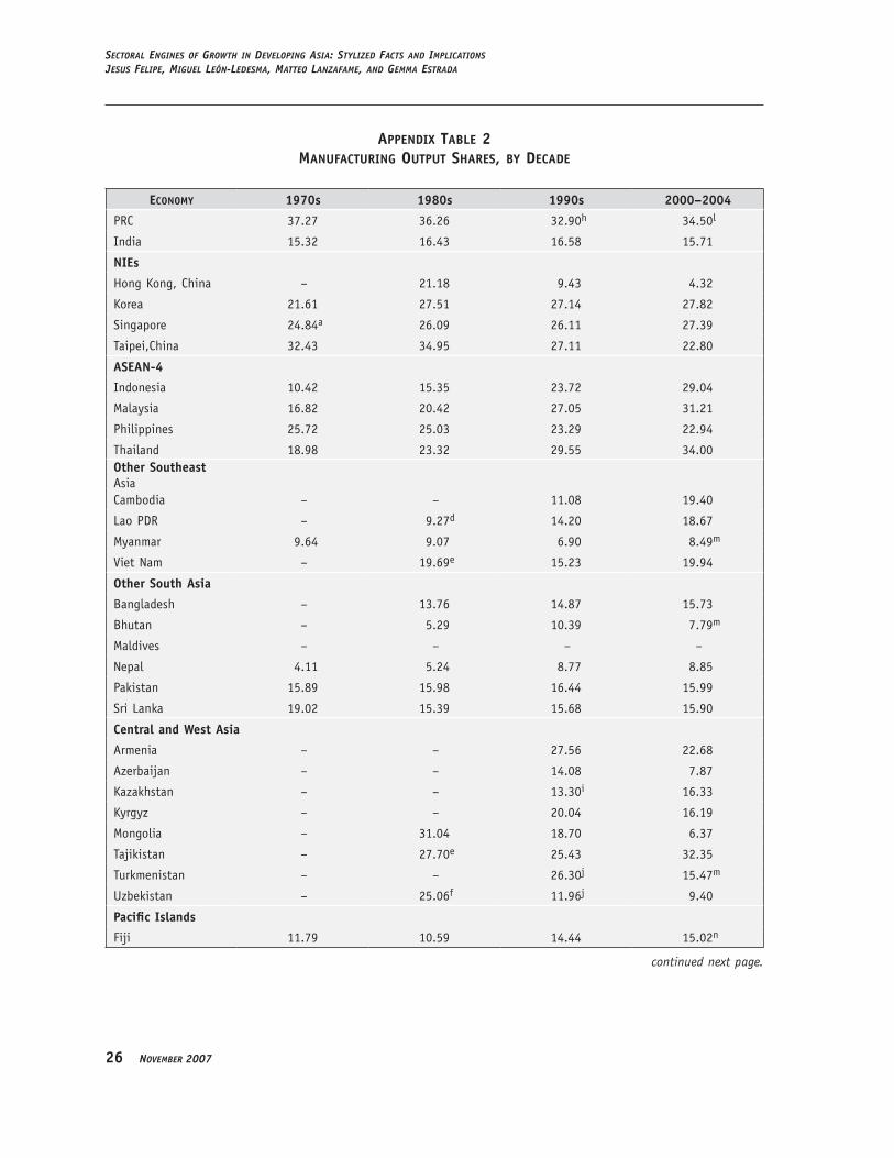
�� November 2007
Sectoral eNgiNeS of growth iN DevelopiNg aSia: StylizeD factS aND implicatioNSJeSuS felipe, miguel leóN-leDeSma, matteo laNzafame, aND gemma eStraDa
appenDix table 2manufacturing output ShareS, by DecaDe
economy 1�70s 1��0s 1��0s �000–�00�
PRC 37.27 36.26 32.90h 34.50l
India 15.32 16.43 16.58 15.71
NIEs
�ong �ong, China – 21.18 9.43 4.32
�orea 21.61 27.51 27.14 27.82
Singapore 24.84a 26.09 26.11 27.39
Taipei,China 32.43 34.95 27.11 22.80
AsEAN-�
Indonesia 10.42 15.35 23.72 29.04
Malaysia 16.82 20.42 27.05 31.21
Philippines 25.72 25.03 23.29 22.94
Thailand 18.98 23.32 29.55 34.00other southeast AsiaCambodia – – 11.08 19.40
��ao PDR – 9.27d 14.20 18.67
Myanmar 9.64 9.07 6.90 8.49m
�iet Nam – 19.69e 15.23 19.94
other south Asia
Bangladesh – 13.76 14.87 15.73
Bhutan – 5.29 10.39 7.79m
Maldives – – – –
Nepal 4.11 5.24 8.77 8.85
Pakistan 15.89 15.98 16.44 15.99
Sri ��anka 19.02 15.39 15.68 15.90
Central and West Asia
Armenia – – 27.56 22.68
Azerbaijan – – 14.08 7.87
�azakhstan – – 13.30i 16.33
�yrgyz – – 20.04 16.19
Mongolia – 31.04 18.70 6.37
Tajikistan – 27.70e 25.43 32.35
Turkmenistan – – 26.30j 15.47m
Uzbekistan – 25.06f 11.96j 9.40
Pacific Islands
�iji 11.79 10.59 14.44 15.02n
continued next page.
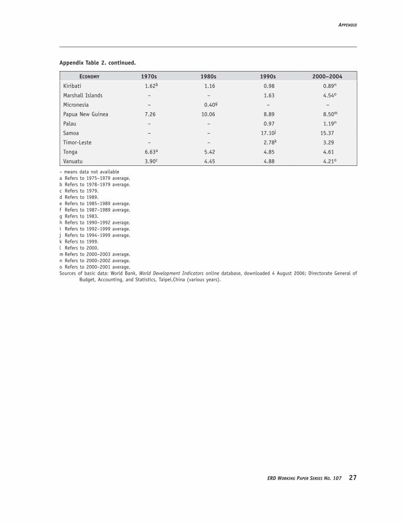
erD workiNg paper SerieS No. 107 �7
economy 1�70s 1��0s 1��0s �000–�00�
�iribati 1.62b 1.16 0.98 0.89n
Marshall Islands – – 1.63 4.54o
Micronesia – 0.40g – –
Papua New ��uinea 7.26 10.06 8.89 8.50m
Palau – – 0.97 1.19n
Samoa – – 17.10j 15.37
Timor-��este – – 2.78k 3.29
Tonga 6.63a 5.42 4.85 4.61
�anuatu 3.90c 4.45 4.88 4.21o
– means data not availablea Refers to 1975–1979 average.b Refers to 1978–1979 average.c Refers to 1979.d Refers to 1989.e Refers to 1985–1989 average.f Refers to 1987–1989 average.g Refers to 1983.h Refers to 1990–1992 average.i Refers to 1992–1999 average.j Refers to 1994–1999 average.k Refers to 1999.l Refers to 2000.m Refers to 2000–2003 average.n Refers to 2000–2002 average.o Refers to 2000–2001 average.Sources of basic data: World Bank, World Development Indicators online database, downloaded 4 August 2006; Directorate ��eneral of
Budget, Accounting, and Statistics, Taipei,China (various years).
Appendix table �. continued.
appeNDix
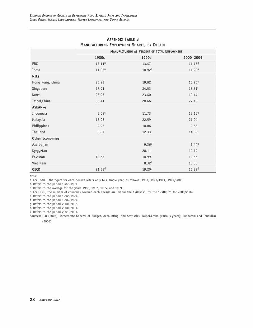
�� November 2007
Sectoral eNgiNeS of growth iN DevelopiNg aSia: StylizeD factS aND implicatioNSJeSuS felipe, miguel leóN-leDeSma, matteo laNzafame, aND gemma eStraDa
appenDix table 3manufacturing employment ShareS, by DecaDe
manufacturing aS percent of total employment
1��0s 1��0s �000–�00�
PRC 15.11b 13.47 11.16g
India 11.05a 10.92a 11.22a
NIEs
�ong �ong, China 35.89 19.02 10.20h
Singapore 27.91 24.53 18.31i
�orea 23.93 23.40 19.44
Taipei,China 33.41 28.66 27.40
AsEAN-�
Indonesia 9.68c 11.73 13.15g
Malaysia 15.95 22.59 21.94
Philippines 9.93 10.06 9.65
Thailand 8.87 12.33 14.58
other Economies
Azerbaijan 9.36e 5.44g
�yrgyztan 20.11 19.19
Pakistan 13.66 10.99 12.66
�iet Nam 8.32f 10.33
oECD 21.58d 19.20d 16.89d
Note:a �or India, the figure for each decade refers only to a single year, as follows: 1983, 1993/1994, 1999/2000.b Refers to the period 1987–1989.c Refers to the average for the years 1980, 1982, 1985, and 1989.d �or OECD, the number of countries covered each decade are: 18 for the 1980s; 20 for the 1990s; 21 for 2000/2004.e Refers to the period 1992–1999.f Refers to the period 1996–1999.g Refers to the period 2000–2002.h Refers to the period 2000–2001.i Refers to the period 2001–2003.Sources: I��O (2006); Directorate-��eneral of Budget, Accounting, and Statistics, Taipei,China (various years); Sundaram and Tendulkar
(2006).

erD workiNg paper SerieS No. 107 ��
appe
nDi
x ta
ble
4av
erag
e to
tal
gDp
grow
th a
nD
Sect
oral
gro
wth
by
Deca
De
econ
omy
1�70
s1�
�0s
1��0
s�0
00s0
�
tota
lag
ri-
cult
ure
inDu
Stry
Serv
iceS
tota
lag
ri-
cult
ure
inDu
Stry
Serv
iceS
tota
lag
ri-
cult
ure
inDu
Stry
Serv
iceS
tota
lag
ri-
cult
ure
inDu
Stry
Serv
iceS
PRC
5.90
2.39
8.22
5.79
9.23
5.14
10.0
511
.93
9.53
4.23
12.1
08.
918.
763.
289.
779.
36
Indi
a2.
520.
313.
844.
455.
714.
186.
576.
285.
532.
955.
607.
345.
561.
686.
097.
30
NIE
s
�on
g �o
ng,
Chin
a8.
73–
––
6.97
––
–3.
66–
––
4.62
..
.
�ore
a7.
953.
6913
.57
6.32
7.32
1.58
8.98
7.23
5.96
0.96
6.41
5.76
5.23
0.09
6.95
4.17
Sing
apor
e8.
402.
759.
138.
387.
18–3
.74
6.17
7.75
7.32
–3.4
98.
137.
143.
98–1
.44
2.82
4.66
ASEA
N-4
Indo
nesi
a7.
484.
159.
808.
416.
144.
017.
086.
624.
512.
065.
674.
534.
543.
414.
065.
50
Mal
aysi
a7.
564.
968.
298.
635.
653.
466.
446.
016.
880.
118.
067.
745.
083.
675.
524.
86
Phili
ppin
es5.
813.
937.
895.
021.
891.
500.
583.
412.
711.
452.
403.
634.
242.
913.
655.
19
Thai
land
6.80
4.06
9.40
6.63
7.02
4.39
8.67
6.82
4.94
0.42
6.91
4.50
4.97
3.39
6.12
4.13
othe
r so
uthe
ast
Asia
Cam
bodi
a6.
571.
5915
.92
5.06
��ao
PDR
3.86
6.
184.
8611
.24
5.44
5.78
3.56
9.82
5.89
�iet
Nam
4.36
7.
143.
829.
967.
396.
893.
719.
596.
10
othe
r so
uth
Asia
Bang
lade
sh0.
82–0
.31
1.26
2.15
3.17
1.58
4.41
3.72
4.69
3.32
6.75
4.15
5.28
3.55
6.83
5.35
Bhut
an–
––
–7.
13
6.21
3.33
8.28
7.25
6.24
..
.
Mal
dive
s–
––
––
––
––
––
–6.
48.
..
Nepa
l2.
520.
72–
–3.
953.
477.
303.
464.
752.
426.
975.
973.
433.
732.
333.
16
Paki
stan
4.04
1.84
5.40
6.05
6.62
4.24
7.86
6.52
3.88
4.05
4.56
4.43
4.05
2.04
4.67
4.57
Sri
��ank
a4.
152.
363.
395.
004.
042.
254.
115.
125.
122.
496.
545.
433.
880.
353.
275.
41
cont
inue
d ne
xt p
age.
appeNDix
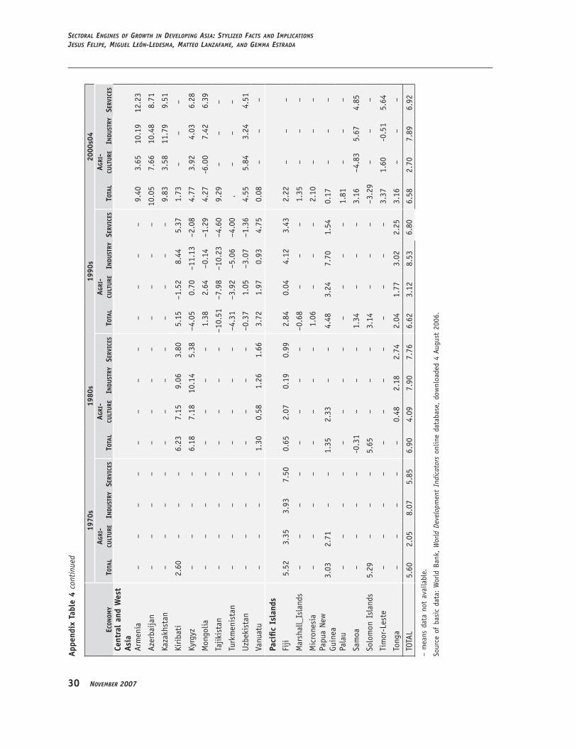
�0 November 2007
Sectoral eNgiNeS of growth iN DevelopiNg aSia: StylizeD factS aND implicatioNSJeSuS felipe, miguel leóN-leDeSma, matteo laNzafame, aND gemma eStraDa
econ
omy
1�70
s1�
�0s
1��0
s�0
00s0
�
tota
lag
ri-
cult
ure
inDu
Stry
Serv
iceS
tota
lag
ri-
cult
ure
inDu
Stry
Serv
iceS
tota
lag
ri-
cult
ure
inDu
Stry
Serv
iceS
tota
lag
ri-
cult
ure
inDu
Stry
Serv
iceS
Cent
ral
and
Wes
t As
ia
Arm
enia
––
––
––
––
––
––
9.40
3.65
10.1
912
.23
Azer
baija
n–
––
––
––
––
––
–10
.05
7.66
10.4
88.
71
�aza
khst
an–
––
––
––
––
––
–9.
833.
5811
.79
9.51
�iri
bati
2.60
––
–6.
237.
159.
063.
805.
15–1
.52
8.44
5.37
1.73
––
–
�yrg
yz–
––
–6.
187.
1810
.14
5.38
–4.0
50.
70–1
1.13
–2.0
84.
773.
924.
036.
28
Mon
golia
––
––
––
––
1.38
2.64
–0.1
4–1
.29
4.27
-6.0
07.
426.
39
Tajik
ista
n–
––
––
––
––1
0.51
–7.9
8–1
0.23
–4.6
09.
29–
––
Turk
men
ista
n–
––
––
––
––4
.31
–3.9
2–5
.06
–4.0
0.
––
–
Uzb
ekis
tan
––
––
––
––
–0.3
71.
05–3
.07
–1.3
64.
555.
843.
244.
51
�anu
atu
––
––
1.30
0.58
1.26
1.66
3.72
1.97
0.93
4.75
0.08
––
–
Paci
fic
Isla
nds
�iji
5.52
3.35
3.93
7.50
0.65
2.07
0.19
0.99
2.84
0.04
4.12
3.43
2.22
––
–
Mar
shal
l_Is
land
s–
––
––
––
––0
.68
––
–1.
35–
––
Mic
rone
sia
––
––
––
––
1.06
––
–2.
10–
––
Papu
a Ne
w
��uin
ea3.
032.
71–
–1.
352.
33–
–4.
483.
247.
701.
540.
17–
––
Pala
u–
––
––
––
––
––
–1.
81–
––
Sam
oa–
––
–-0
.31
––
–1.
34–
––
3.16
–4.8
35.
674.
85
Solo
mon
Isl
ands
5.29
––
–5.
65–
––
3.14
––
––3
.29
––
–
Tim
or-��
este
––
––
––
––
––
––
3.37
1.60
-0.5
15.
64
Tong
a–
––
––
0.48
2.18
2.74
2.04
1.77
3.02
2.25
3.16
––
–
TOTA
��5.
602.
058.
075.
856.
904.
097.
907.
766.
623.
128.
536.
806.
582.
707.
896.
92
– m
eans
dat
a no
t av
aila
ble.
Sour
ce o
f ba
sic
data
: W
orld
Ban
k, W
orld
Dev
elop
men
t In
dica
tors
onl
ine
data
base
, do
wnl
oade
d 4
Augu
st 2
006.
Appe
ndix
tab
le �
con
tinu
ed
erD workiNg paper SerieS No. 107 �1
REFERENCEs
Abramovitz, M. 1986. “Catching-Up, �orging Ahead and �alling Behind.” Journal of Economic History 46:386–406.
———. 1993. “The Origins of the Post-War Catch-Up and Convergence Boom.” In J. �agerberg, B. �erspagen, and N. von Tunzelmann, eds., The Dynamics of Technology, Trade and Growth. Aldershot: Edward Elgar.
ADB. 2007. Asian Development Outlook 2007. Asian Development Bank, Manila.Aghion, P., and P. �owitt. 1992. “A Model of ��rowth through Creative Destruction.” Econometrica 60:323–
51.Anant, T. C. A., R. �asan, P. Mohapatra, R. Nagaraj, and S.�. Sasikumar. 2006. “��abor Markets in India: Issues
and Perspectives.” In J. �elipe and R. �asan, eds., Labor Markets in Asia: Issues and Perspectives. ��ondon: Palgrave Macmillan for the Asian Development Bank.
Banister, J. 2005. “Manufacturing Employment in China.” Monthly Labor Review (July):11-29Baumol, W. J., S. A. Batey Blackman, and E. Wolff. 1985. “Unbalanced ��rowth Revisited: Asymptotic Stagnancy
and New Evidence.” The American Economic Review 75:4(September):806–17.———. 1989. Productivity and American Leadership: The Long View. Cambridge: MIT Press.�agerberg, J. 2000. “Technological Progress, Structural Change and Productivity ��rowth: A Comparative Study.”
Structural Change and Economic Dynamics 11:393–411.�orni M., M. �allin, M. ��ippi, and ��. Reichlin. 2001. “The ��eneralized �actor Model: Identification and
Estimation.” The Review of Economics and Statistics 82(3):540–54.��erschekron, A. 1962. Economic Backwardness in Historical Perspective: A Book of Essays. Cambridge, MA:
Belknap Press.�aldor, N. 1966. Causes of the Slow Rate of Growth in the United Kingdom. Cambridge: Cambridge University
Press.———. 1967. Strategic Factors in Economic Development. New ��ork State School of Industrial and ��abor
Relations, Cornell University, New ��ork.��eamer, E. E., and J. ��evinsohn. 1995. “International Trade Theory: The Evidence.” In ��. ��rossman and �.
Rogoff, eds., The Handbook of International Econ. �ol III. Amsterdam: Elsevier Science B.�.��ucas, R. E. Jr. 1988. “On the Mechanics of Economic Development.” Journal of Monetary Economics 22:3–
42.McCombie, J. S. ��. 1980. “On the Quantitative Importance of �aldor�s ��aws.” Bulletin of Economic Research
32:102–12.McCombie, J. S. ��., M. Pugno, and B. Soro, eds. 2002. Productivity Growth and Economic Performance: Essays
on Verdoorn’s Law. �oundmills and New ��ork: Palgrave Macmillan.Midelfart-�narvik, �. �., Overman, �. ��., Redding, S. J. and �enables, A. J. 2000. The ��ocation of European
Industry. Economic Papers 142, European Commission Directorate-��eneral for Economic and �inancial Affairs, Brussels.
Nelson, R. R., and ��. Wright. 1992. “The Rise and �all of American Technological ��eadership: The Post-war Era in �istorical Perspective.” Journal of Economic Literature 30:1931–64.
Nixson, �. I. 1990. “Industrialization and Strcutural Change in Developing Countries.” Journal of International Development 2(2, July):310–33.
Pedroni, P. 2000. “�ully Modified O��S for �eterogeneous Cointegrated Panels.” Advances in Econometrics 15:93–130.
Pieper, U. 2000. “Deindustrialisation and the Social and Economic Sustainability Nexus in Developing Countries: Cross-country Evidence on Productivity and Employment.” The Journal of Development Studies 36(4, April):66–99.
Rodrik, D. 2006. “Industrial Development: Stylized �acts and Policies.” John �. �ennedy School of ��overnment. Available: http://ksghome.harvard.edu/~drodrik/industrial%20development.pdf.
refereNceS
�� November 2007
Sectoral eNgiNeS of growth iN DevelopiNg aSia: StylizeD factS aND implicatioNSJeSuS felipe, miguel leóN-leDeSma, matteo laNzafame, aND gemma eStraDa
Romer, P.M. 1986. “Increasing Returns and ��ong Run ��rowth.” Journal of Political Economy 94:1002–37.———. 1990. “Endogenous Technological Change.” Journal of Political Economy 98:71–102.Ros, J. 2000. Development Theory & The Economics of Growth. Ann Arbor: The University of Michigan Press.Rowthorn, R., and R. Rawasmany. 1997. Deindustrialization: Causes and Implications. IM� Working Paper
p9/42, International Monetary �und, Washington, DC.———. 1999. “��rowth, Trade and Deindustrialization.” IMF Staff Papers 46(1):18–41.Sundaram, �. and S. Tendulkar. 2006. “Changing Structue of India Workforce, Quality of Employment and
Real Earnings, 1983-2000” in Institute for �uman Development, India: Meeting the Employment Challenge, Conference on ��abour and Employment Issues, July 27-29, New Delhi.
Temple, J. 1999. “The New ��rowth Evidence.” Journal of Economic Literature 37:112–56.Timmer, M. P., and A. Szirmai. 2000. “Productivity ��rowth in Asian Manufacturing: The Sstructural Bonus
�ypothesis Examined.” Structural Change and Economic Dynamics 11:371–92.Wells, �., and A. P. Thirlwall. 2003. “Testing �aldor�s ��rowth ��aws across the Countries of Africa.” African
Development Review 15(2-3):89–105.