about the presenter - universiteit · pdf fileprocter & gamble - baby care r&d about...

1

Fluid Flow in Absorbing Porous Media

Presented at the Marie Curie Workshopfor Flow and Transport in Industrial Porous Media

Nov. 12 – 16, 2007University Utrecht, The Netherlands

Procter & Gamble © 2007

Dr. Mattias SchmidtResearch Fellow – Victor Mills Society, Procter & Gamble - Baby Care R&D

ABOUT THE PRESENTER

Dr. Mattias Schmidt is a Research Fellow and member of the Victor Mills Society.

He joined P&G with a PhD in Physics from University of Leipzig and has worked in the area of fluid flow, absorbent core design and super-

b b t l d l t f th


absorbent polymer development for more than 16 years.

2

Outline

• P&G at a glance• Importance of Modeling & Simulation for R&D• Fluid Flow in Hygiene Products

– Introduction– Some FemCare examples– Impact of hysteresis on fluid (re-)distribution– Introduction to Diaper Cores and AGM


– Impact of AGM swelling on fluid flow• Typical challenges and opportunities for

collaboration

It began with Soap & Candles…

James GambleSoap MakerFOUNDED IN

•Fifth Oldest Company on the

William ProcterCandle Maker

1837


Company on the Fortune 50…


3

P&G In a Glance

•Sales of $ 68.2 billions

P&G at a glance– 170 years old– Annual Sales of more than $ 70

billion•Nearly 300 brands in more than 160 countries

•22 global brands with sales of over $ 1 billion

•Workforce of 140.000

– Nearly 300 brands in more than 160 countries

– 22 global brands with sales of over $ 1 billion

– Worldwide workforce of 140,000– 140 plants and 25 R&D centers

globally


•3 billions people touched everyday by P&G products

•Spends more than $5 million a day on R&D

globally– Spend more than $ 2 billion a year

on R&D


22 Billion-Dollar Brands

4

How do we define Innovation?

Innovation is the blend of“What’s

What’sNeeded?

What’sPossible?

•Consumer•Customer•Competition

•TechnologyConsumer Delight

Needed” with “What’s Possible”


Leading Edge Innovation

•Set up first product research lab in U.S. in 1890

‘Innovation is our Lifeblood’

in 1890

•Currently have 24,000 active Patents, receive 3800 per year.


•Invest over $2.0 Billion per year in R&D

y

5

Importance of Modeling & Simulation for R&D


Typical Challenges

Products must perform when used … But face Fundamental

Engineering Contradictions.

•Materials … strong but soft—even wet, stretch not break, breath but contain, break…not tear/selectively tear.


•Liquids … mixtures can’t separate, must stay where applied…but dispense easily.

•Packages … design is key, be strong but light, never leak but open easily.

6

Scales of Modeling

ComputationalChemistry

hrs

days

MechEng/ChE(Closed Form

Industrial Eng/Operations Resrch

(Statistical, DiscreteEvent, Agent Based)

Time

ns

ms

sec

Molecular

Coarse Grain or Mesoscale Modeling –Polymers

Continuum or Finite DifferenceFinite Element

y (Closed FormEquations)


Distance

Quantum Chemistry

- subatomic

Mechanics-atoms,

molecules

angstroms micronsnm mm m

Computer AidedEngineering (CAE)

km

fs

Computing Hardware Performance

‘Moore’s Law’

SNL ‘Red Storm’1015 Petaflops

ORNL ‘peta-Scale’

LLNL ASCI ‘White’

U.S. DOE ‘Leadership’

Gigaflops

Megaflops

1012 TeraflopsLANL“Blue Mountain”

Leadership Class Machines


Kilaflops

20001990 2010

P&G’s1st, 2nd, & 3rd

Generations

7

Thermal Performance


Current Body Scans

Current Full Body Scans


8

Validating the Fit Model

Full Body Scan Current Model


Bone Modeling

Women’sBone Health…


Based on these results, three factors are critical for addressing bone strength in osteoporosis:

(1) reduction in the stress risers, (2) targeted increase of bone volume, (3) preservation of architecture.

9

Fluid Flow in Absorbent Hygiene Products


Typical Liquid Handling Processes

Macroscopic Liquid Handling• Absorption• Release

~mm~cm,~m

• Distribution / Redistribution• Storage / Retention (i.e. stop flow)• Provide Barrier (i.e. stop flow)

Microscopic Liquid Handling• Contact Angle & Wetting


Contact Angle & Wetting• Deposition / Spreading• Dewatering• Condensation• Filtration

µm

10

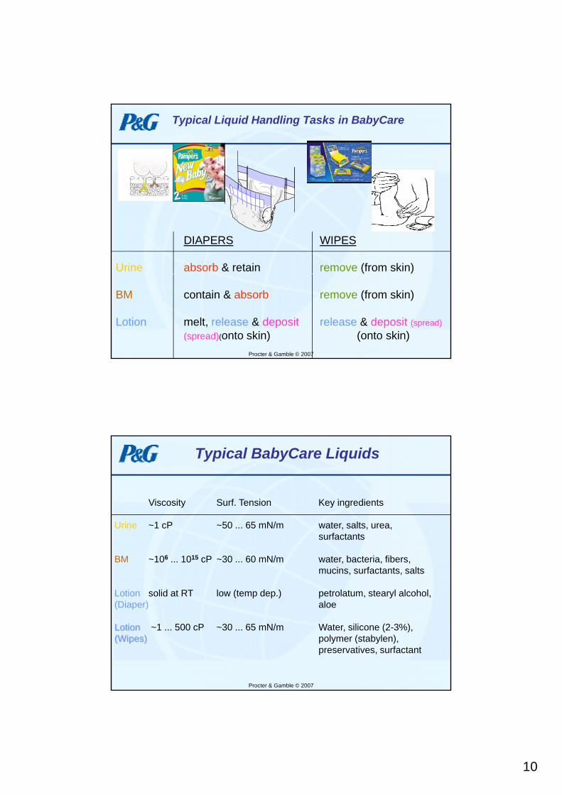
Typical Liquid Handling Tasks in BabyCare

DIAPERS WIPES

Urine absorb & retain remove (from skin)


BM contain & absorb remove (from skin)

Lotion melt, release & deposit release & deposit (spread)(spread)(onto skin) (onto skin)

Typical BabyCare Liquids

Viscosity Surf. Tension Key ingredients

Urine ~1 cP ~50 ... 65 mN/m water, salts, urea, surfactants

BM ~106 ... 1015 cP ~30 ... 60 mN/m water, bacteria, fibers, mucins, surfactants, salts

Lotion solid at RT low (temp dep.) petrolatum, stearyl alcohol,(Diaper) aloe


(Diaper) aloe

Lotion ~1 ... 500 cP ~30 ... 65 mN/m Water, silicone (2-3%), (Wipes) polymer (stabylen),

preservatives, surfactant

11

BM distribution

Example – BM viscosity varies widely

Vi it [P ]

All BM’sRunny BM’s

Urine


Viscosity [Pa s](at zero shear)

10-3 100 103 106 109 1012

For comparison:Viscosity range of some Other products

Porous Media Flow

• Simulation of fluid flow in porous structures applied to product design of „paper products“

e.g. Diapers, Feminine Pads, Towels, Swiffer, Wipes, Make-up-Applications, Olay Facial Wipes ...

• Being used to develop new designs and new materials


materials

• Richards equation is a typical formulation

12

Examples of Fluid Flow in Porous Mediafor Aborbent Hygiene Products


Absorbent Core Modeling

O ti i ti

Model Input:• Core design• Raw material prop´s• Test protocol

Model Output:• Acquisition time• Liquid distribution / partitioning

• Capillary Pressure*• Flow Patterns*

Optimization

Validation


Experimental (Lab):• Acquisition time• Liquid distribution / partitioning

Simulation* Additional insights that can experimentally not easily detected.

13

Example: X-Ray Analysis

Front

j (y-direction, CD)ct

ion,

MD

)

Front

j (y-direction, CD)ct

ion,

MD

)j=0 .. 10j=0 .. 10

0 1 2 3 4 5 6 7 8 9 10

0 0.058 0.056 0.058 0.057 0.059 0.059 0.063 0.058 0.057 0.058 0.061

Ray

Imag

e –

Inte

nsity

i,ji (x-

dire

c

Ray

Imag

e –

Inte

nsity

i,ji (x-

dire

c

i=0

.. 40

ding

Dis

tribu

tion

–Lo

adi,j

i=0

.. 40

ding

Dis

tribu

tion

–Lo

adi,j

Weigh diaper – total load LLo adMFRAME

123

45

67

89

10

111213

141516

1718

1920

21222324

252627282930

3132333435

0.058 0.066 0.069 0.073 0.081 0.091 0.103 0.084 0.078 0.081 0.0670.057 0.07 0.09 0.106 0.104 0.104 0.138 0.114 0.113 0.13 0.0750.058 0.117 0.138 0.175 0.164 0.16 0.205 0.2 0.19 0.174 0.128

0.067 0.153 0.261 0.353 0.448 0.578 0.553 0.367 0.336 0.271 0.0870.059 0.103 0.345 0.632 0.772 0.856 0.844 0.727 0.567 0.323 0.076

0.056 0.207 0.624 0.901 1.061 1.153 1.157 1.052 0.835 0.414 0.090 0.298 0.888 1.054 1.25 1.371 1.395 1.295 1.126 0.592 0.062

0.056 0.324 1.058 1.249 1.409 1.636 1.666 1.453 1.101 0.453 0.0570.058 0.304 1.153 1.331 1.579 1.768 1.75 1.681 1.376 0.406 0.0620.062 0.218 1.149 1.465 1.723 1.838 1.871 1.873 1.575 0.228 0.056

0.06 0.127 0.998 1.441 1.721 1.809 1.867 1.851 1.546 0.141 00.061 0.125 1.061 1.459 1.624 1.725 1.771 1.729 1.063 0.075 0.0540.063 0.165 1.086 1.456 1.563 1.562 1.542 1.51 0.803 0.061 0

0.063 0.172 0.927 1.214 1.197 1.241 1.142 0.819 0.562 0.066 0.0570.063 0.116 0.561 0.629 0.733 0.833 0.763 0.74 0.206 0.063 0.0570.062 0.069 0.262 0.827 1.054 1.061 1.059 0.959 0.199 0.062 0.055

0.06 0.065 0.444 1.007 1.087 1.256 1.208 1.128 0.555 0.063 0.0550.06 0.104 0.777 1.172 1.291 1.236 1.232 1.153 0.579 0.063 0.055

0.06 0.138 0.941 1.405 1.704 1.765 1.526 1.346 0.699 0.072 0.0550.061 0.252 1.081 1.525 1.813 1.843 1.679 1.44 1.015 0.117 0.057

0.061 0.337 1.205 1.607 1.859 1.935 1.867 1.647 1.19 0.349 0.0560.062 0.405 1.272 1.622 1.818 1.962 1.843 1.554 1.126 0.326 0.0560.063 0.472 1.199 1.531 1.745 1.886 1.721 1.419 0.912 0.213 0.0570.064 0.526 1.05 1.332 1.56 1.617 1.487 1.21 0.875 0.193 0.057

0.083 0.5 0.857 0.999 1.124 1.145 1.069 1.052 0.72 0.143 0.0550.134 0.619 0.865 0.975 1.058 1.074 1.034 0.965 0.613 0.14 0.0540.118 0.642 0.859 0.989 1.01 1.054 0.937 0.814 0.398 0.094 0.0540.062 0.516 0.843 1.025 1.023 0.885 0.686 0.512 0.264 0.186 0.0610.06 0.367 0.788 0.974 0.949 0.649 0.419 0.203 0.177 0.13 0.055

0.059 0.139 0.591 0.692 0.619 0.349 0.165 0.131 0.117 0.118 0.059

0.062 0.086 0.089 0.135 0.172 0.109 0.134 0.115 0.088 0.075 00.059 0.083 0.082 0.07 0.086 0.119 0.122 0.098 0.087 0.072 0.0550.056 0.062 0.08 0.083 0.132 0.186 0.128 0.084 0.075 0.078 0.0540.061 0.064 0.072 0.083 0.109 0.155 0.118 0.079 0.067 0.068 0.0540.057 0.063 0.068 0.069 0.087 0.124 0.107 0.075 0.062 0.063 0.055

=


Back

X-R

Back

X-R

Load

Load 36

37

3839

40

0.055 0.06 0.066 0.072 0.089 0.129 0.107 0.07 0.064 0.06 0.0540.056 0.058 0.067 0.071 0.086 0.11 0.096 0.069 0.068 0.061 0

0.055 0.061 0.067 0.071 0.087 0.104 0.1 0.074 0.063 0.061 0.0550.058 0.062 0.071 0.072 0.073 0.089 0.084 0.072 0.069 0.063 0.058

0.055 0 0 0 0 0 0 0 0 0 0.055

Quantitative determination of load distribution

Upper CoreLower CoreInsult

Examples from FemCare*Dual layer structure

Procter & Gamble © 2007* Not limited to FemCare – could be other dual layer structure

14

1 layer homogeneous structure2 layer homogeneous structure

3D simulations – fluid generated at corner

1 layer homogeneous structure Top – high permeability, low PcapBottom – low permeability, high Pcap


No hysteresis, gravity included Hysteresis, gravity included

Fluid generated at corner


Key learning:• for limited fluid amounts we need to include hysteresis to describe product behavior

15

Why does liquid not spread over an entire fabric?

... Capillary hysteresis stops wicking

... How can we control stain size?

Procter & Gamble © 2007time

TRI/Autoporosimeter (PVD)

- Capillary pressure as a Pc

PC Control

Gas

function of saturation (measure saturation as a function of pressure)

- Data used to generate:-Pore volume distribution-Cumulative volume

m(t)Measure

reservoirscale

Sample

Frit/Membrane


-Saturation vs. Pressure

Fluids used include Hexadecane, H2O/Surfactant, Salt Solutions

Typically 2 steps: 1) absorption with dry material 2) drainage 3) absorption with wetted material

16

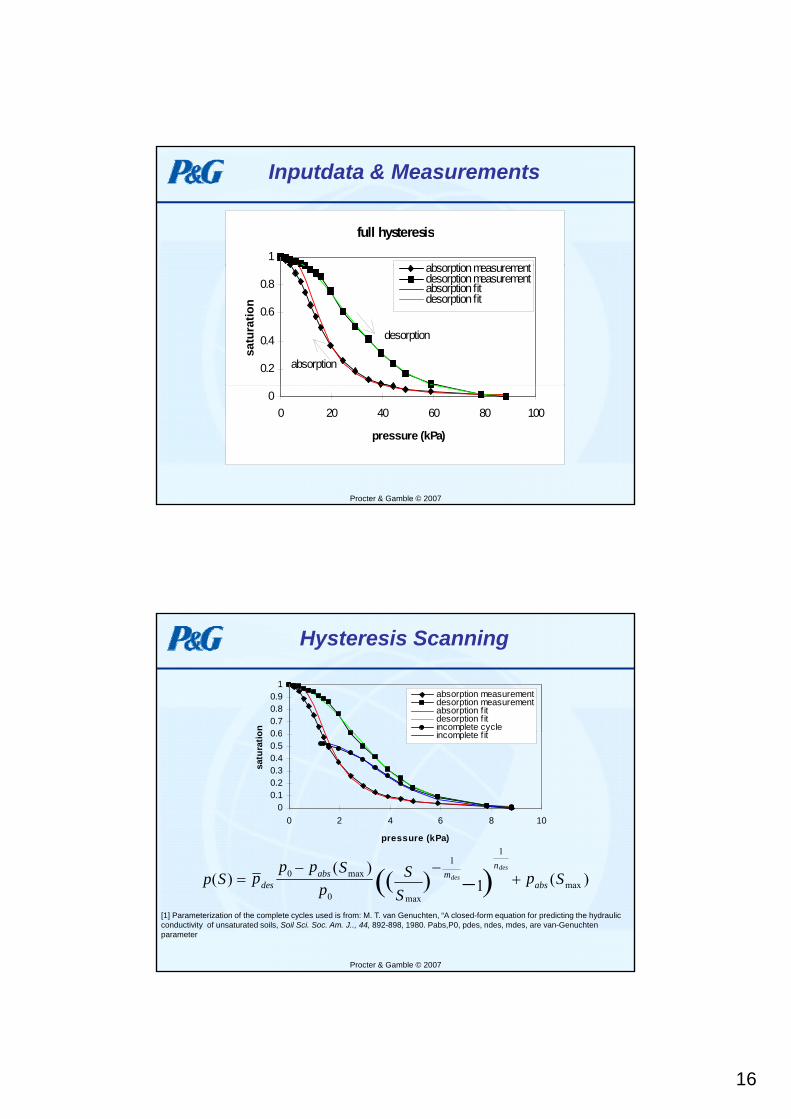
Inputdata & Measurements

full hysteresis1

absorptionmeasurement

0.2

0.4

0.6

0.8

satu

ratio

nabsorption measurementdesorption measurementabsorption fitdesorption fit

absorption

desorption


00 20 40 60 80 100

pressure (kPa)

Hysteresis Scanning

0 60.70.80.9

1

on

absorption measurementdesorption measurementabsorption f itdesorption f itincomplete cyclei l t f it

00.10.20.30.40.50.6

0 2 4 6 8 10

pressure (kPa)

satu

ratio incomplete f it

1


p S pp p S

pS

Sp Sdes

absn

mabs

desdes( )

( )( )max

maxmax( )( )=

− −+−0

0

11

1

[1] Parameterization of the complete cycles used is from: M. T. van Genuchten, “A closed-form equation for predicting the hydraulicconductivity of unsaturated soils, Soil Sci. Soc. Am. J.., 44, 892-898, 1980. Pabs,P0, pdes, ndes, mdes, are van-Genuchten parameter

17

Wicking Experiment and Simulation

[ ]nS x t k S

P x S S∂ ∂ ∂( , ) ( )

, , &= ⋅

liquid reservoir

[ ]nt x x

P x S Sc∂ ∂ μ ∂, ,


sample plastic foil

Simulation done in FORTRAN/NAG Library

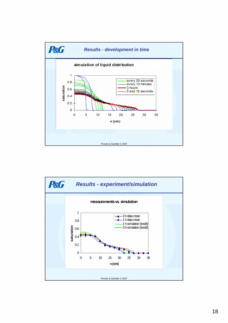
Results - development in time


18

Results - development in time


Results - experiment/simulation

measurements vs. simulation

1

0.2

0.4

0.6

0.8

1

satu

ratio

n

3 h data mean1 h data mean1 h simulation (test8)3 h simulation (test8)


00 5 10 15 20 25 30 35

x (cm)

19

Predictions - different load

different percentages of maximum loadsimulation 3 hours

1

0.2

0.4

0.6

0.8

satu

ratio

n

8.25 %

reference 17.9 %

30.90%


00 5 10 15 20 25 30 35

x (cm)

Predictions - reduced hysteresis

reduced hysteresis simulation 3 hours1

1/2 hysteresis

0.2

0.4

0.6

0.8

satu

ratio

n

yreference full hysteresis1/4 hysteresiszero hysteresis


00 5 10 15 20 25 30 35

x (cm)

20

Predictions - permeability

different permeability

1

k k Sb= ⋅0b ~ 4.5 for reference

0.2

0.4

0.6

0.8

1

satu

ratio

n

0.5 k0reference2 k00.5 b (b=2)


00 5 10 15 20 25 30 35

x (cm)

Key Learnings

• Hysteresis leads to a stop of the liquid front, the higher the load the less impact of hysteresis

• Decrease of b greatly improves liquid distribution

• Increase of k0 improves liquid distribution

• Reduction to zero hysteresis shows good distribution but reducing hysteresis has


essentially no impact

21

Diaper Core Technology

Diaper (from Side )Diaper (from Side )

Front ofNappy

Back ofNappy

Inside SurfaceWaist feature

Acquisition PatchLotion Stripes Topsheet


Nappy ppy

Outside SurfaceBacksheet Storage Core (homogenous

blend of AGM and cellulose)Dusting Layer

How does a diaper work?Liquid Handling Tasks of diaper Cores

Acquisition &

Liquid

•Nonwoven Layer•Modified Cellulose Fibers

Acquisition &Distribution


FibersStorage Core:AGM + Cellulose

22

Final

How does a diaper work?Liquid Handling Tasks of diaper Cores

FinalAbsorption

• AGM can absorb about 30 times of its own weight, whereas cellulose can absorb only around 4 times of its own weight.


absorb only around 4 times of its own weight.

AGM 70%

Pampers Core

Airfelt 30%

What is AGM?

AGM = absorbent gelling material= superabsorber, supersorber, superabsorbent polymer (SAP),= superabsorbent material (SAM)= superabsorbent material (SAM), = hydrogels, hydrogel-forming polymers

• White granulate powder with particles ranging from 45 mm to 850 mm.

• A cross-linked poly-acrylate, about 75% neutralized with Na+ - Ions.

Enables s per thin diaper designs at impro ed leakage and dr ness performance


• Enables super-thin diaper designs at improved leakage and dryness performance (move from 100% pulp cores to ~30% pulp cores today).

23

AGM Chemistry

CO2H COOCOO

OC = O

R - C - Et

O

CO2H

CO2HCO2HNa+

Na+

Na+

Na+

Na+


• AGM = absorbent gelling material• white powder made of lightly crosslinked polymer networks• based on water soluble hydrophilic polymer• crosslinked to connect the chains of the polymer: “elastic springs”• liquid is absorbed via diffusion … forms a hydrogel much like gelatin

• Take up urine and lock it away – as much as possible!

Function of AGM

• Take up urine and lock it away – as much as possible! (Storage Capacity)

• Transport urine within itself, e.g. within a swollen gel bed.(Permeability)

• Work reasonably fast.


y(Speed)

24

Controlled Swelling / High Permeability

Uncontrolled Swelling/ Gel Blocking

What is „Gel Blocking“?

UrineUrine


Poor permeability causesunder-utilized AGM

Gel-Blocking Demo


25

Higher Crosslinked ShellShell creates

Surface Crosslinking

L C li k d B lk

tangential forces„balloon effect“


Lower Crosslinked Bulk

• surface crosslinking maintains particle shape during swelling• improves permeability and swelling capacity

Fluid Flow in AGM-containing cores

• AGM absorbs liquid „away from the pores between AGM particles and fibers“– Acts like a „sink term“ in the fluid flow equation of the pore structureActs like a „sink term in the fluid flow equation of the pore structure– Liquid absorbed into each AGM particle by diffusion / osmotic process– Swelling of AGM changes the pore structure

• Described as „two types of liquid“ – m1: „mobile fluid“ in the pore structure– m2: „immobile“ fluid in the gel

• Requires modified equation systemm2

Fluid absorbed by swellable material


Requires modified equation system– Richards equation extended by „sink term“– Key properties of pore structure now depend on m2

– Additional equation for absorption of liquid into the gel phase

m1

Fluid in pores of the swellable material

26

Example Equations (1D, horizontal)

2212

1211

1

)(

)),(),,(()),(),,((),(

xm

txmtxmDx

mtxmtxmD

xttxm

=⎟⎠

⎞⎜⎝

⎛ ++∂∂

∂∂

∂∂

∂∂

• Calculates liquid movement through absorbent core and AGM

max

2max021

),()),(),,(((

mtxmm

ACtxmtxmSf AGM−

⋅⋅⋅⋅−= τ

max

2max021

2 ),()),(),,((( ),(

mtxmm

ACtxmtxmSft

txmAGM

−⋅⋅⋅⋅+= τ

∂∂


• Calculates liquid movement through absorbent core and AGM• Predict liquid handling properties of absorbent cores.

optimize AGM properties for specific core designsoptimize core designs for specific AGMs

• This also applies in 2D/3D

Example: Typical Assumptions

1) The fluid-swellable composite material comprises fluid-swellable particulate material and may comprise voids between the particles of said material; liquid is either in said voids or inside the fluid-swellable particulate material.

2) Liquid movement in one dimension only (e.g. x- direction).2) Liquid movement in one dimension only (e.g. x direction).

3) The fluid-swellable (composite) material swells only transverse (perpendicular) to the direction of liquid movement (swelling only in y or z direction).

4) Once liquid is inside the fluid-swellable material it remains inside.

5) The liquid does not move inside the fluid-swellable material (e.g. liquid that enters the fluid-swellable material at point x will always stay at point x).

6) Liquid can distribute inside the voids; this distribution is governed by Darcy’s law and


6) Liquid can distribute inside the voids; this distribution is governed by Darcy s law and liquid mass conservation.

7) The flow direction is horizontal, such that gravity can be neglected.

The model may however also be applied to a two dimensional or three dimensional situation.

27

Example: Multilayer Core Structure incl. AGM

• Pictures show snapshots of fluid in pores (~saturation) and fluid in AGM at two different times after a gush onto a pre-loaded core

• Illustrates how upper acquistition layers and interstitials are being dewatered and fluid is absorbed into the AGMn

Short time after gush „In equilibrium“ after gush

Inte

rstitial s

atur

ation


AGM

load

I

Challenges & Opportunities for Collaboration


28

Typical Challenges

• Designs are long / large area but very thin– Difficult to mesh properly (balance of speed / accuracy)

• Product developers want the answers fast– Computation time, stability of simulations new algorithms– Need to be able to run lots of simulations

• Extreme material properties– Typical porosities ~90% or higher– Large parameter contrast in K(S) and Pc(S) and hysteresis– Properties change during use (swelling, external pressure changes)– Thin materials (see below)


• Multiple physical effects– Porous Media Flow– Free Surface Flow– Mechanical Deformation

• Liquids can be difficult– Surfactants – Surface tension as function of time, Surfactant Transport– Non-newtonian effects – most equations do not apply to high porosities

Opportunities for Collaboration

• Fluid flow models in presence of– Thin layers– Hydrophobic layers / bridging

M t f K(S)*• Measurement of K(S)*• Design materials with target K(S)• Large parameter contrast and initially very dry materials• Initial wetting behavior of very dry materials (analogy to

soil)• Experimental characterization of surfactant release and

transport in porous media


p p• Micromodels to predict K(S, pext), Pc(S, pext), n(pext)• Multiple capillary pressure cycles (absorption /

desorption) implementation in models* The relative permeability of materials as a function of capillary pressure and/or saturation is currently determined by comparing the virtual spatial map of saturation predicted in the virtual test simulations to the physical spatial map of saturation measured in the physical test environment and altering one or more of the absorbent-fluid interaction properties the absorbent used in the virtual test environment, until the spatial maps of saturation compare favorably. We are looking for more direct measurement techniques.

29

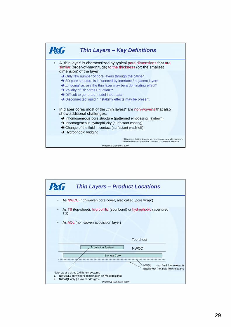
Thin Layers – Key Definitions

• A „thin layer“ is characterized by typical pore dimensions that aresimilar (order-of-magnitude) to the thickness (or: the smallest dimension) of the layer.

Only few number of pore layers through the calipery p y g p3D pore structure is influenced by interface / adjacent layers„bridging“ across the thin layer may be a dominating effect*Validity of Richards Equation?*Difficult to generate model input dataDisconnected liquid / Instability effects may be present

• In diaper cores most of the „thin layers“ are non-wovens that also h dditi l h ll


show additional challenges:Inhomogeneous pore structure (patterned embossing, laydown)Inhomogeneous hydrophilicity (surfactant coating)Change of the fluid in contact (surfactant wash-off)Hydrophobic bridging

* This means that the flow may not be just driven by capillary pressure differential but also by absolute pressures / curvature of meniscus.

Thin Layers – Product Locations

• As NWCC (non-woven core cover, also called „core wrap“)

• As TS (top-sheet): hydrophilic (spunbond) or hydrophobic (apertured TS)TS)

• As AQL (non-woven acquisition layer)

Acquisition System

Top-sheet

NWCC


Storage Core

NWDL (not fluid flow relevant)Backsheet (not fluid flow relevant)

NWCC

Note: we are using 2 different systems1. NW AQL / curly fibers combination (in most designs)2. NW AQL only (in low-tier designs)

30

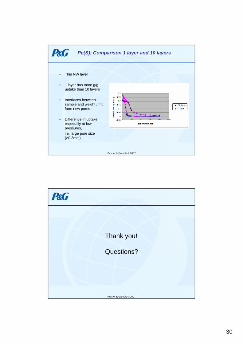
Pc(S): Comparison 1 layer and 10 layers

• Thin NW layer

• 1 layer has more g/g uptake than 10 layers

• Interfaces between sample and weight / frit form new pores

Diff i t k


• Difference in uptake especially at low pressures, i.e. large pore size (>0.3mm)

Thank you!

Questions?


31

Additional Information – Terms and Abbreviations


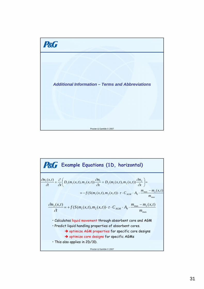
Example Equations (1D, horizontal)

2212

1211

1

)(

)),(),,(()),(),,((),(

xm

txmtxmDx

mtxmtxmD

xttxm

=⎟⎠

⎞⎜⎝

⎛ ++∂∂

∂∂

∂∂

∂∂

• Calculates liquid movement through absorbent core and AGM

max

2max021

),()),(),,(((

mtxmm

ACtxmtxmSf AGM−

⋅⋅⋅⋅−= τ

max

2max021

2 ),()),(),,((( ),(

mtxmm

ACtxmtxmSft

txmAGM

−⋅⋅⋅⋅+= τ

∂∂


• Calculates liquid movement through absorbent core and AGM• Predict liquid handling properties of absorbent cores.

optimize AGM properties for specific core designsoptimize core designs for specific AGMs

• This also applies in 2D/3D.

32

Example: Typical Assumptions

1) The fluid-swellable composite material comprises fluid-swellable particulate material and may comprise voids between the particles of said material; liquid is either in said voids or inside the fluid-swellable particulate material.

2) Liquid movement in one dimension only (e.g. x- direction).2) Liquid movement in one dimension only (e.g. x direction).

3) The fluid-swellable (composite) material swells only transverse (perpendicular) to the direction of liquid movement (swelling only in y or z direction).

4) Once liquid is inside the fluid-swellable material it remains inside.

5) The liquid does not move inside the fluid-swellable material (e.g. liquid that enters the fluid-swellable material at point x will always stay at point x).

6) Liquid can distribute inside the voids; this distribution is governed by Darcy’s law and


6) Liquid can distribute inside the voids; this distribution is governed by Darcy s law and liquid mass conservation.

7) The flow direction is horizontal, such that gravity can be neglected.

The model may however also be applied to a two dimensional or three dimensional situation.

where (a) x is the space dimension (b) t is the time (c) m1 is the amount of liquid in voids per length. (d) m2 is the amount of liquid in fluid-swellable material, e.g. particles, per length

f∂

(l) ),( 21 mmPc is the capillary pressure. This is in general a function of m1 and m2. (see the method section below)

(m) μ is the viscosity of the liquid - (see the method section below)

(n) 1m

Pc

∂∂

is the partial derivative of Pc in respect to m1

P∂(e)

tf∂∂

is the partial derivative of any variable f(x,t) in respect to time t, e.g.

1

tm∂∂

is the partial derivative of m1 in respect to time t

(f) xf∂∂

is the partial derivative of any variable f(x,t) in respect to space x, e.g.

1

xm∂∂

is the partial derivative of m1 in respect to space x

(g) )),(),,(( 2111 txmtxmDD = is the diffusivity 1 defined as

1

21212211

),(),()(),(

mmmPmmk

mAmmD cliq ∂

∂μ

ρ ⋅⋅⋅=

(h) )),(),,(( 2122 txmtxmDD = is the diffusivity 2 defined as

(o) 2m

Pc

∂∂

is the partial derivative of Pc in respect to m2

(p) τ is the swelling speed (see the method section below). In general τ is a function of m2

(q) mmax is the maximum capacity (see method section below)

(r) material) swellable fluid(dry Volume

material) swellable fluid(dry Mass=AGMC is the fluid-swellable

material concentration, determined as ratio between mass and dry volume, where the mass is determined by weighing the fluid-swellable material, and the dry volume is calculated by determining caliper, length and width of the dry fluid-swellable composite material

(s) S is the liquid saturation in the voids and can be expressed as function of m1

and m2. )()(

),( 121 mAmn

mmmS

⋅⋅=ρ


( ) )),(),,(( 2122 txmtxm y

2

21212212

),(),()(),(m

mmPmmkmAmmD cliq ∂

∂μ

ρ ⋅⋅⋅=

(i) liqρ is the density of the liquid

(j) )( 2mA is the cross section area. This is a function of m2 and porosity (n).

))(),,(()( 222 mntxmAmA = . From volume conservation it is possible to

express )( 2mA as ( )

( ) liq

txmA

txmnn

mAρ

),(),((1

1)( 2

02

max2 +⋅

−−

=

(k) ),( 21 mmk is the permeability. This is in general a function of m1 and m2. (see the methods section below)

)()( 22 mAmnliq ⋅⋅ρ(t) )),(),,((( 21 txmtxmSf is an empirical function expressing the dependency

of the swelling kinetics on saturation in the voids. This function can be approximated with several equations, an example is to assume SSf =)(

(u) n is the porosity and is function of m2. (see method section below) (v) maxn is the value of porosity in dry conditions.

about the presenter - universiteit · pdf fileprocter & gamble - baby care r&d about...

Documents