Conservative high order semi-Lagrangian finite difference WENO methods for

advection in incompressible flow

Jing-Mei Qiu1 and Chi-Wang Shu 2

Abstract

In this paper, we propose a semi-Lagrangian finite difference formulation for approximat-

ing conservative form of advection equations with general variable coefficients. Compared

with the traditional semi-Lagrangian finite difference schemes [4, 21], which approximate

the advective form of the equation via direct characteristics tracing, the scheme proposed

in this paper approximates the conservative form of the equation. This essential difference

makes the proposed scheme naturally conservative for equations with general variable coef-

ficients. The proposed conservative semi-Lagrangian finite difference framework is coupled

with high order essentially non-oscillatory (ENO) or weighted ENO (WENO) reconstructions

to achieve high order accuracy in smooth parts of the solution and to capture sharp inter-

faces without introducing spurious oscillations. The scheme is extended to high dimensional

problems by Strang splitting. The performance of the proposed schemes is demonstrated by

linear advection, rigid body rotation and swirling deformation. As the information is propa-

gating along characteristics, the proposed scheme does not have CFL time step restriction of

the Eulerian method, allowing for a more efficient numerical realization for many application

problems.

Keywords: advection in incompressible flow; conservative scheme; semi-Lagrangian meth-

ods; WENO reconstruction.

1Department of Mathematical and Computer Science, Colorado School of Mines, Golden, 80401. E-mail:jingqiu@mines.edu. Research supported by NSF grant number 0914852 and Air Force Office of ScientificResearch grant number FA9550-09-1-0344.

2Division of Applied Mathematics, Brown University, Providence, 02912. E-mail: shu@dam.brown.edu.Research supported by AFOSR grant FA9550-09-1-0126 and NSF grant DMS-0809086.

1

1 Introduction

In this paper, we consider numerically simulating the advection of a scalar density function

u(x, t) in an incompressible flow with the specified velocity field a(x, t) in general high spatial

dimensions, x ∈ Rd, where d is the spatial dimension. The evolution of u(x, t) is governed

by the advection equation

ut + a(x, t) · ∇xu = 0, (1.1)

with the divergence free condition on the velocity field ∇ · a = 0. Equation (1.1) can be

rewritten in a conservative form as

ut +∇x · (a(x, t)u) = 0, (1.2)

due to the divergence free condition of the velocity field a.

Numerical approaches in simulating the advection problem described above can be clas-

sified as three types: Eulerian, Lagrangian and semi-Lagrangian. The Lagrangian type

particle methods evolve the solution by following the trajectories of some sampled macro-

particles, while the Eulerian approach evolves the PDE itself, e.g. equation (1.1) or (1.2), on

a fixed numerical grid. The semi-Lagrangian approach is a mixed approach of Lagrangian

and Eulerian in the sense that it has a fixed numerical grid; however in each time step evolu-

tion it evolves the PDEs by propagating information along characteristics. As the Eulerian

approach, the semi-Lagrangian method can be designed to be of very high order accuracy

[21], an advantage when compared with the Lagrangian approach which suffers the low order

O(1/√

N), with N being the number of sampling macro-particles, due to the statistical noise

in the initial sampling of macro-particles. On the other hand, because of the evolution mech-

anism, the semi-Lagrangian method does not suffer the CFL time step restriction as in the

Eulerian approach, allowing for extra large time step evolution therefore less computational

effort. In this paper, a scheme is considered to be semi-Lagrangian, if it has the following

three components.

1. A solution space: the solution space can be point values, integrated mass (cell aver-

ages), or a piecewise polynomial function living on a fixed numerical grid, correspond-

ing to the semi-Lagrangian finite difference scheme [5, 21, 16], semi-Lagrangian finite

volume scheme [13] and the characteristic Galerkin method [7, 18] respectively.

2

2. In each of the time step evolution, information is propagated along characteristics.

In this step, there is no explicit numerical discretization of ddt

. The only numerical

error in time comes from tracing characteristics backward in time in order to find their

origin at tn. Usually, a high order interpolation or reconstruction procedure, which

determines the spatial accuracy of the scheme, is applied to recover the information

among discrete information on the solution space.

3. Lastly, the evolved solution is projected back onto the solution space, updating the

numerical solution at tn+1.

The semi-Lagrangian approach is very popular in the numerical weather prediction [26],

the plasma simulations [25, 1, 2, 16, 28, 3, 21], among many others. In the kinetic simu-

lation of plasma, a very popular approach is the Strang split semi-Lagrangian method first

proposed by Cheng and Knorr [6]. The idea is that, rather than solving the truly multi-

dimensional genuinely nonlinear equations, Cheng and Knorr applied the Strang splitting

to decouple the high dimensional nonlinear Vlasov equation into a sequence of 1-D ‘linear’

equations on a rectangular grid. The advantage of performing such a splitting is that the

decoupled 1-D advection equations are linear and are much easier to resolve numerically.

On the other hand, the numerical error in time is dominated by the splitting error which

is of order O(∆t2). In this paper, we will adopt the Strang splitting idea, and decouple

the high dimensional advection problem (1.2) into a sequence of conservative 1-D advection

equation. We remark that in the context of Strang splitting equation (1.1) or (1.2), or the

kinetic equation, semi-Lagrangian finite difference schemes that evolve point values would

be advantageous when compared with the semi-Lagrangian finite volume schemes or char-

acteristic Galerkin methods. A scheme working on grid points would not suffer the ‘at best’

second order spatial error, because of the shearing of velocity field, as those schemes working

over a cell region. In this paper, we consider the semi-Lagrangian finite difference method

with Strang splitting on equation (1.2).

The traditional semi-Lagrangian finite difference schemes [3, 21, 16] usually approximate

the advective form of equation by tracing characteristics backward in time and using an

interpolation algorithm to recover the information among grid points. For example, in the

context of Strang splitting, the equation (1.1) is split into a sequence of 1-D advective

3

equations

ut + ai(x, t)uxi= 0, i = 1, · · · , d (1.3)

each of which is approximated by a semi-Lagrangian finite difference scheme. Such scheme

has decent performance in many problems [3]. However, the total mass, which is an analyt-

ically conserved quantity, is not necessarily conserved numerically for such a scheme. This

might lead to serious problems, for example in the relativistic Vlasov-Maxwell simulation

[16]. In this paper, we consider a new formulation of semi-Lagrangian scheme that approxi-

mates the conservative form, rather than the advective form of the PDE. Specifically, in the

context of Strang splitting, the equation (1.1) (or equivalently the equation (1.2)) is split

into a sequence of 1-D conservative equations

ut + (ai(x, t)u)xi= 0, i = 1, · · · , d (1.4)

each of which is approximated by a conservative scheme.

An important component of the semi-Lagrangian scheme is the interpolation or recon-

struction procedure in recovering information among grid points, which determines the spa-

tial accuracy of the scheme. In the literature, there are a variety of choices [12, 28] such as

piecewise parabolic method (PPM) [10], positive and flux conservative method (PFC) [13],

spline interpolation [11], cubic interpolation propagation (CIP) [27], ENO/WENO interpo-

lation or reconstruction [17, 23, 5, 21]. In this paper, we will apply the ENO or WENO

procedures to ensure high order spatial accuracy in smooth regions and to avoid spurious

oscillations at discontinuities.

In summary, we propose a new semi-Lagrangian finite difference scheme approximating

the conservative form of the 1-D advection equation (1.4) and the multi-D advection equation

(1.2) by a conservative Strang splitting. Since most of our discussion will be focused on a

split 1-D problem, without loss of generality, we will work on the following 1-D equation

ut + (a(x, t)u)x = 0. (1.5)

We remark that solving the truly multi-dimensional problem, rather than the Strang split

1-D equation, is highly nontrivial and is going to be our future research. On the other hand,

there is a recent numerical approach in overcoming the dimensional splitting error in the

4

framework of spectral deferred correction methods [8]. The idea over there might have the

potential of being applied to our split scheme here.

The paper is organized as follows. Section 2 is a review of finite difference WENO scheme

coupled with the method of lines procedure. Section 3 gives the semi-Lagrangian scheme

for approximating equation (1.5) with a(x, t) being a constant. Section 4 generalizes the

scheme to the equations with general variable coefficient a(x, t). Section 5 demonstrates the

performance of the proposed schemes by linear advection, rigid body rotation and swirling

deformation. Section 6 gives the conclusion and indicates a few possible directions for future

research.

2 Review of finite difference WENO scheme coupled

with the method of line approach

In this section, we briefly review the finite difference WENO spatial discretization coupled

with the method of lines (MOL) procedure for a 1-D conservative form of advection equation

(1.5), with the initial condition u(x, t = 0) = u0(x). For simplicity, we assume periodic

boundary condition. The purpose of this review section is to recall the idea behind the high

order finite difference WENO scheme, especially the sliding average function h(x), which is

also used in the proposed semi-Lagrangian finite difference scheme in Sections 3 and 4. The

readers are referred to [9, 23] for more details. In this paper, we adopt the following spatial

discretization of the domain [a, b]

a = x 12

< x 32, · · · , < xN+ 1

2= b, (2.1)

where Ii = [xi− 12, xi+ 1

2], i = 1, · · · , N are uniform numerical cells with the center of the

cell xi = 12(xi+ 1

2+ xi− 1

2) and the cell size ∆x = xi+ 1

2− xi− 1

2= (b − a)/N . We denote

ui(t) = u(xi, t) and uni = u(xi, t

n) with tn = n∆t.

The finite difference scheme evolves the point values of the solution uiNi=1 by approxi-

mating the equation (1.5) directly. The scheme is of conservative form

d

dtui = − 1

∆x(fi+ 1

2− fi− 1

2), (2.2)

where the numerical flux

fi+ 12

= f(ui−p, · · · , ui+q)

5

is consistent with the physical flux f(u) = a(x, t)u and is Lipschitz continuous with respect

to all arguments. The stencil ui−p, · · · , ui+q is chosen to be upwind biased. Especially,

when a(x, t) ≥ 0, one more point from the left (p = q) will be taken to reconstruct fi+ 12; when

a(x, t) < 0, one more point from the right (p = q−2) will be taken. When a(x, t) changes sign

over the domain, then a flux splitting, e.g. the Lax-Friedrich flux splitting can be applied [23].

The spatial accuracy of the scheme is determined by how well 1∆x

(fi+ 12− fi− 1

2) approximates

(a(x, t)u)x. To obtain a high order approximation, Shu and Osher [24] introduced a sliding

average function h(x), such that

1

∆x

∫ x+∆x2

x−∆x2

h(ξ)dξ = a(x, t)u(x, t), (2.3)

for a fixed t. Taking the x derivative of the above equation gives

1

∆x

(h(x +

∆x

2)− h(x− ∆x

2)

)= (au)x. (2.4)

Therefore the numerical flux fi+ 12

in equation (2.2) can be taken as h(xi+ 12), which can be

reconstructed from neighboring cell averages of h(x), hj = 1∆x

∫Ij

h(ξ)dξ(2.3)= a(xj, t)u(xj, t),

j = i − p, · · · , i + q by WENO reconstruction [23]. Equation (2.2) is further discretized in

time by a method of line (MOL) procedure, the most popular of which is the third order

TVD Runge-Kutta method [14].

Remark 2.1. An essential difference between the semi-Lagrangian scheme proposed in this

paper and the finite difference WENO reviewed above is the way of evolving solution in

time. There is explicit time discretization, e.g. the Runge-Kutta method, in the method

of line approach, while in the semi-Lagrangian scheme, there is no explicit discretization

of time derivative ddt

. Rather, information is propagated along characteristics and the only

error in time comes from tracing characteristics backward in time. As a result, the accuracy

and stability issues involved in the temporal evolution of semi-Lagrangian scheme are quite

different from those in the method of line approach. In this paper, we only consider the

situation when the backward characteristic tracing can be performed either exactly (when a

is a constant) or by a high order ODE solver (when a = a(x, t)).

6

3 Semi-Lagrangian scheme for 1-D advection with con-

stant coefficient

We start by introducing the proposed semi-Lagrangian formulation for 1-D equation

ut + (au)x = 0, (3.1)

where a is a constant. The formulation presented in this section will be extended to the case

of variable coefficient a = a(x, t) in the next section.

3.1 Basic formulation

We propose a semi-Lagrangian finite difference scheme by integrating equation (3.1), which

is of conservative form, over [tn, tn+1],

u(x, tn+1) = u(x, tn)−

(∫ tn+1

tnau(x, τ)dτ

)x

.

Evaluating the above equation at the grid point xi gives

un+1i = un

i −

(∫ tn+1

tnau(xi, τ)dτ

)x

= uni −Fx|x=xi

(3.2)

where we let

F(x) =

∫ tn+1

tnau(x, τ)dτ. (3.3)

We introduce a function H(x), whose sliding average is F(x), i.e.

F(x) =1

∆x

∫ x+∆x2

x−∆x2

H(ξ)dξ. (3.4)

Taking the x derivative of the above equation gives

Fx =1

∆x

(H(x +

∆x

2)−H(x− ∆x

2)

).

Therefore the equation (3.2) can be written in a conservative form as

un+1i = un

i −1

∆x(H(xi+ 1

2)−H(xi− 1

2)), (3.5)

7

where H(xi+ 12) is called the flux function. Notice that, from equation (3.1) to (3.5) there

is no numerical discretization involved yet. Similar to the idea in finite difference WENO

scheme, H(xi+ 12) can be reconstructed from its neighboring cell averages

Hj =1

∆x

∫ xj+1

2

xj− 1

2

H(ξ)dξ(3.4)= F(xj), j = i− p, · · · , i + q. (3.6)

Now the remaining question is how to obtain F(xi)Ni=1 (or HiN

i=1).

From Figure 3.1, we observe that, at each of the grid points at time level tn+1, say

(xi, tn+1), there exists a backward characteristic line, with the foot located on time level tn

at x?i . When a is constant, these backward characteristic lines are straight and parallel with

slope 1a

in the x-t plane. Moreover, along each of these characteristic lines the solution re-

mains constant, i.e. u(xi, tn+1) = u(x?

i , tn), which is the fact used in most of semi-Lagrangian

finite difference schemes in the literature. We propose to take a slightly different approach

here. We denote the region Ωi to be the triangular region bounded by the three points

(xi, tn+1), (xi, t

n) and (x?i , t

n), see Figure 3.1. We apply the integral form of equation (3.1)

over the region Ωi, ∫Ωi

ut + (au)x = 0. (3.7)

By the Divergence Theorem, the left hand side of the above equation can be written in the

following explicit form∫Ωi

ut + (au)x =

∫∂Ωi

u · nt + au · nx

= −∫ xi

x?i

u(ξ, tn)dξ +

∫ tn+1

tnau(xi, τ)dτ. (3.8)

From equation (3.7) and (3.8),

Hi = F(xi) =

∫ tn+1

tnau(xi, τ)dτ =

∫ xi

x?i

u(ξ, tn)dξ, (3.9)

where∫ xi

x?i

u(ξ, tn)dξ can be reconstructed from uni N

i=1.

In summary, a semi-Lagrangian finite difference scheme in evolving the solution from tn

to tn+1 to approximate equation (3.1) can be designed as follows.

Step 1: At each of the grid points at time level tn+1, say (xi, tn+1), trace the characteristic

back to time level tn at x?i . When a is constant, x?

i = xi − a∆t.

8

v r r r v v v v v r r r v tn+1

v r r r v v v

Ωi

x?i

6

v v r r r v tn

x0 xi−2 xi−1 xi xi+1 xi+2 xN

Figure 3.1: Semi-Lagrangian scheme approximates equation (1.5).

Step 2: Reconstruct HiNi=1 with Hi

(3.9)=∫ xi

x?i

u(ξ, tn)dξ from uni N

i=1. We use R1 to denote

this reconstruction procedure

Hi = R1[x?i , xi](u

ni−p1

, · · · , uni+q1

), (3.10)

where i− p1, · · · , i+ q1 indicate the stencil used in the reconstruction, and R1[a, b] indicates

the reconstruction of∫ b

au(ξ, t)dξ.

Step 3: Reconstruct H(xi+ 12)N

i=0 from HiNi=1. We use R2 to denote this reconstruction

procedure

H(xi+ 12) = R2(Hi−p2 , · · · , Hi+q2), (3.11)

where i− p2, · · · , i + q2 indicate the stencil used in the reconstruction.

Step 4: Update the solution un+1i N

i=1 by equation (3.5) with H(xi± 12) computed in the

previous step.

Remark 3.1. In the proposed scheme, the propagation of the information along character-

istics is not as explicit as those in the traditional semi-Lagrangian finite difference scheme

un+1i = u(x?

i , tn). However, by applying the Divergence Theorem on equation (3.7), the infor-

mation on [x?i , xi]× tn is propagated over to the region of xi× [tn, tn+1]. Such propagation

of information is in the spirit of semi-Lagrangian. When a is constant, there is no error in

locating the root of characteristic x?i , therefore there is no error in time at all in the pro-

posed scheme. The accuracy of the scheme is solely determined by the spatial reconstruction

procedure outlined in Steps 2 and 3 above.

9

Remark 3.2. The basic formulation of the scheme above can be generalized to the case

when a is a variable coefficient a(x, t) without difficulty, see Section 4.

In the following two subsections, we discuss the situation when a first order (Section 3.2)

and general high order (Section 3.3) spatial reconstructions are applied to recover the infor-

mation between grid point values.

3.2 A first order scheme

To better understand the scheme, we start with a first order reconstruction, which is discussed

as two separate cases |a|∆t ≤ ∆x and |a|∆t > ∆x. Despite its simplicity, the first order

scheme gives us insight in designing the high order extension in Section 3.3.

The procedure for a first order scheme can be designed as following. In Step 2, we

reconstruct Hi =∫ xi

x?i

u(ξ, tn)dξ where the underlying function u(x, tn) is approximated by a

piecewise constant function

u(x, tn) = uni , on [xi−1, xi], (3.12)

and in Step 3, we design the flux

H(xi+ 12) = Hi, (3.13)

regardless of the sign of a.

1. Consider |a|∆t ≤ ∆x. When a ≥ 0, x?i ≤ xi, then

H(xi+ 12) = Hi =

∫ xi

x?i

u(ξ, tn)dξ ≈ (xi − x?i )u

ni = a∆tun

i .

Plug these flux functions into equation (3.5) gives the scheme

un+1i = un

i −a∆t

∆x(un

i − uni−1) = un

i − ξ(uni − un

i−1), (3.14)

where ξ = a∆t∆x

. The scheme reduces to the prototype of the first order finite difference

upwind scheme. Especially when a∆t = ∆x, the scheme in equation (3.14) reduces to

un+1i = un

i−1, indicating the exact shifting of grid points. In this case, the solution is

exactly evolved, with no numerical error in either time or space. Similar result holds

when a < 0 and x?i > xi. Plug flux functions

H(xi+ 12) = Hi =

∫ x?i

xi

u(ξ, tn)dξ ≈ (x?i − xi)u

ni+1 = |a|∆tun

i+1

10

into equation (3.5) gives

un+1i = un

i + ξ(uni+1 − un

i ), (3.15)

with ξ = |a|∆t∆x

, which is the prototype of the first order finite difference upwind scheme.

Especially when |a|∆t = ∆x, the scheme reduces to un+1i = un

i+1.

2. Consider |a|∆t > ∆x. When a ≥ 0 and xi−x?i > ∆x. Let i? to be the index such that

x?i ∈ (xi?−1, xi? ] and ξ =

xi?−x?i

∆x

H(xi+ 12) = Hi =

∫ xi

x?i

u(ξ, tn)dξ ≈i∑

j=i?+1

unj ∆x + (xi? − x?

i )uni?

Plug these flux functions into equation (3.5) gives the scheme

un+1i = un

i −1

∆x

((

i∑j=i?+1

unj ∆x + (xi? − x?

i )uni?)− (

i−1∑j=i?

unj ∆x + (xi?−1 − x?

i−1)uni?−1)

)

= uni −

1

∆x(∆x(un

i − uni?) + ξ∆x(un

i? − uni?−1))

= uni? − ξ(un

i? − uni?−1) (3.16)

One observation from the equation above is that, although information is integrated

along x?i to xi to compute Hi, the final form of the scheme (3.16) only involves the

information around the foot of characteristics x?i . Similar result holds for a < 0.

Remark 3.3. In our scheme, neither the reconstruction R1 nor R2 depends on the wind

direction (the sign of a(x, t)). The information on wind direction is automatically recovered

by locating x?i via characteristics tracing, see the derivation of equation (3.14) and (3.15).

This consistent treatment regardless of the sign of a is crucial, when dealing with the situation

that a(x, t) changes sign in Section 4.

Remark 3.4. Another symmetric way of approximation can be designed as following. In

Step 2, the underlying function u(x, tn) is approximated by a piecewise constant function

u(x, tn) = uni−1, on [xi−1, xi]; and in Step 3, H(xi+ 1

2) = Hi+1, regardless of the sign of a.

With this approximation, the first order semi-Lagrangian scheme ends up to be the same as

that from the reconstruction (3.12) and (3.13), i.e. equation (3.14) for a ≥ 0 and equation

(3.15) for a < 0.

11

3.3 High order schemes with WENO reconstructions

In this section, we will extend the first order scheme in the previous section to high order.

We will first consider the case when |a|∆t < ∆x, in which we will first consider linear high

order extension of the scheme for smooth problem. Then we will incorporate the WENO

mechanism to deal with solutions with discontinuities. After that we will extend the scheme

to the case when |a|∆t ≥ ∆x. The algorithm is summarized in Section 3.3.4. In this

subsection, we will focus our discussion on the case of a ≥ 0. For the case of a < 0, we

will omit the details of the reconstruction procedure for brevity, but only provide necessary

formulas for implementation convenience.

3.3.1 High order linear reconstructions: |a|∆t < ∆x

To extend the first order scheme to high order, we would like to make the reconstruction

operators R1 and R2 in equation (3.10) and (3.11) to be of high order. A direct way of doing

this is to include more points in the reconstruction stencil in (3.10) and (3.11). Take a third

order scheme for example. We will extend the reconstruction (3.12) by using uni−1, u

ni , u

ni+1

as the reconstruction stencil to reconstruct u(x, tn) on [xi−1, xi]; we will extend (3.13) by

using Hi−1,Hi,Hi+1 as the reconstruction stencil, regardless of the sign of the advection

coefficient a. One problem with such implementation is that the reconstruction stencil is too

widely spread. Specifically, when a ≥ 0 and a∆t ≤ ∆x, five points ui−2, ui−1, ui, ui+1, ui+2

are involved to reconstruct the third order flux function H(xi+ 12). More seriously, the scheme

is linearly unstable. To remedy the problem, we observe that in the case of linear reconstruc-

tion, the operators R1 and R2 can be combined together as a linear operator R = R2 R1,

H(xi+ 12) = R(un

i−p, · · · , uni+q) (3.17)

where i − p, · · · , i + q indicate the reconstruction stencil. Such compression of two linear

operators not only makes the reconstruction stencil more compact, but also provides a stable

scheme. Below, we will use third and fifth order reconstructions as examples to illustrate

the reconstruction procedure. The formulas are also a good reference for implementation

purpose.

Third order linear reconstruction. When a ≥ 0, we will use the three-point stencil

12

ui−1, ui, ui+1 to reconstruct Hj with j = i−1, i, i+1 respectively, from which we reconstruct

H(xi+ 12) with third order. Specifically, we integrate the quadratic polynomial interpolating

xi−1, xi, xi+1 over [x?j , xj] = [xj − ξ∆x, xj] as approximation to Hj, with j = i − 1, i, i + 1,

where ξ = a∆t∆x

.

Hi−1 = ∆x

((− 5

12− 1

6(−ξ − 1)3 +

1

4(−ξ − 1)2)un

i−1

+ (ξ +1

3+

1

3(−ξ − 1)3)un

i

+(1

12− 1

6(−ξ − 1)3 − 1

4(−ξ − 1)2)un

i+1

)(3.18)

Hi = ∆x

((1

6ξ3 +

1

4ξ2)un

i−1 + (ξ − 1

3ξ3)un

i + (1

6ξ3 − 1

4ξ2)un

i+1

)(3.19)

Hi+1 = ∆x

((− 1

12− 1

6(1− ξ)3 +

1

4(1− ξ)2)un

i−1

+ (ξ − 1

3+

1

3(1− ξ)3)un

i

+(5

12− 1

6(1− ξ)3 − 1

4(1− ξ)2)un

i+1

), (3.20)

and, as in the linear reconstruction in the finite difference WENO scheme,

H(xi+ 12) = −1

6Hi−1 +

5

6Hi +

1

3Hi+1. (3.21)

Plugging equations (3.18)-(3.20) into equation (3.21) gives

H(xi+ 12) = R(un

i−1, uni , u

ni+1)

= ∆x

((1

6ξ3 − 1

6ξ)un

i−1 + (−1

3ξ3 +

1

2ξ2 +

5

6ξ)un

i + (1

6ξ3 − 1

2ξ2 +

1

3ξ)un

i+1

).= ∆x(C3

1uni−1 + C3

2uni + C3

3uni+1). (3.22)

When a < 0, we will use the three-point stencil ui, ui+1, ui+2 to reconstruct Hj with

j = i−1, i, i+1 respectively, from which we reconstructH(xi+ 12) with third order. Specifically,

we integrate the quadratic polynomial interpolating xi, xi+1, xi+2 over [xj, x?j ] = [xj, xj+ξ∆x]

as approximation to Hj, with j = i−1, i, i+1, where ξ = |a|∆t∆x

. Then we reconstruct H(xi+ 12)

by a linear reconstruction as in equation (3.21). In the end,

H(xi+ 12) = R(un

i , uni+1, u

ni+2) = −∆x(C3

3uni + C3

2uni+1 + C3

1uni+2),

with C3i , i = 1, 2, 3 as defined in equation (3.22), due to the symmetry of the reconstruction.

Details of the reconstruction are omitted here for brevity.

13

Remark 3.5. In the third order reconstruction, we always use the three-point stencil Hi−1, Hi, Hi+1

to reconstruct H(xi+ 12), regardless the sign of advection coefficient a. We use the stencil

ui−1, ui, ui+1 when a ≥ 0 and use ui, ui+1, ui+2 when a < 0 to reconstruct Hj with

j = i− 1, i, i + 1, due to the location of x?i . Similar algorithm is designed for the fifth order

linear reconstruction below.

Fifth order linear reconstruction. Similar procedures can be applied for a fifth order

reconstruction. For brevity, we only present the reconstruction formulas needed in the ac-

tual implementation. When a ≥ 0, we will take the five-point stencil ui−2, · · · , ui+2 to

reconstruct H(xi+ 12),

H(xi+ 12) = R(un

i−2, uni−1, u

ni , u

ni+1, u

ni+2)

= ∆x

((

1

30ξ − 1

24ξ3 +

1

120ξ5)un

i−2

+ (−13

60ξ − 1

24ξ2 +

1

4ξ3 +

1

24ξ4 − 1

30ξ5)un

i−1

+ (47

60ξ +

5

8ξ2 − 1

3ξ3 − 1

8ξ4 +

1

20ξ5)un

i

+ (9

20ξ − 5

8ξ2 +

1

12ξ3 +

1

8ξ4 − 1

30ξ5)un

i+1

+(− 1

20ξ +

1

24ξ2 +

1

24ξ3 − 1

24ξ4 +

1

120ξ5)un

i+2

).= ∆x(C5

1uni−2 + C5

2uni−1 + C5

3uni + C5

4uni+1 + C5

5uni+2). (3.23)

where ξ = a∆t∆x

. When a < 0, we will take the five-point stencil ui−1, · · · , ui+3 to reconstruct

H(xi+ 12),

H(xi+ 12) = R(un

i−1, uni , u

ni+1, u

ni+2, u

ni+3) = −∆x(C5

5uni−1 + C5

4uni + C5

3uni+1 + C5

2uni+2 + C5

1uni+3),

where ξ = |a|∆t∆x

and C5i , i = 1, · · · , 5 are as defined in equation (3.23), due to the symmetry

of the reconstruction.

Remark 3.6. Assume a ≥ 0, when a∆t = ∆x (or ξ = 1), it can be checked that H(xi+ 12) =

∆xuni in both the third order reconstruction (3.22) and the fifth order reconstruction (3.23).

Thus the scheme in equation (3.5) reduces to un+1i = un

i−1, indicating the exact shifting of

grid points. In this case, the solution is exactly evolved, with no numerical error in either

time or space. Indeed, it is proved in Proposition 3.7 below that for general high order

14

reconstructions, such exact evolution is true when a∆t = ∆x. Similar conclusion applies

when a < 0.

Proposition 3.7. Assuming a ≥ 0, when a∆t = ∆x, the flux function H(xi+ 12) = ∆xui for

linear reconstructions of any odd order. In other words, the operator R in equation (3.17)

satisfies

R(uni−p, · · · , un

i+q) = ∆xuni , if a∆t = ∆x

for any reconstruction of an odd order 2k + 1. Therefore the scheme (3.5) is reduced to

un+1i = un

i−1, indicating the exact shifting of grid points. Similar conclusion applies when

a < 0.

Proof. It is known by definition that

Hi =1

∆x

∫ xi+1

2

xi− 1

2

H(ξ, t)dξ, i = 1, · · ·N. (3.24)

Also when a∆t = ∆x,

Hi =

∫ xi

x?i

u(ξ, t)dξ =

∫ xi

xi−1

u(ξ, t)dξ, i = 1, · · ·N. (3.25)

Let j = i − 1 − k. To reconstruct H(xi+ 12) with order 2k + 1, we construct a polynomial

P2k+1(x) of degree 2k + 1 interpolating the primitive function of H at 2k + 2 neighboring

points xj+ 12, · · ·xj+2k+1+ 1

2,

P2k+1(xj+l+ 12) =

∫ xj+l+1

2 Hdξ, l = 0, · · · , 2k + 1;

then we use P ′2k+1(xi+ 1

2) to approximate H(xi+ 1

2). On the other hand, there is a polynomial

Q2k+1(x) of degree 2k + 1 interpolating the primitive function of ∆xu at 2k + 2 neighboring

points xj, · · ·xj+2k+1,

Q2k+1(xj+l) = ∆x

∫ xj+l

udξ, l = 0, · · · , 2k + 1.

From equation (3.24) and (3.25),

P2k+1(xj+l+ 12) = Q2k+1(xj+l), l = 0, · · · , 2k + 1.

15

Since P2k+1(x) and Q2k+1(x) are both polynomials of degree 2k + 1,

P2k+1(x +∆x

2) ≡ Q2k+1(x).

Taking the x derivative of above equation and evaluate it at xi gives

P ′2k+1(xi+ 1

2) = Q′

2k+1(xi) = ∆xu(xi).

Therefore, the numerical flux function H(xi+ 12) = ∆xu(xi). Plugging the flux function into

equation (3.5) gives un+1i = un

i−1, indicating the exact shifting of grid points. This completes

the proof.

3.3.2 High order WENO reconstructions

In general, high order fixed stencil reconstruction of numerical fluxes performs well when

the solution is smooth. However, around discontinuities, spurious oscillations will be in-

troduced. In the following, a nonlinear WENO procedure is introduced for reconstructing

H(xi+ 12). By adaptively assigning weights to neighboring candidate stencils, the WENO

nonlinear reconstruction preserves high order accuracy of the linear scheme around smooth

regions of the solution, while producing a sharp and essentially non-oscillatory capture of

discontinuities. The WENO reconstruction could also be understood as a black box filtering

procedure, based on the fluxes generated from fixed stencil reconstruction introduced above.

The original third and fifth order WENO reconstructions, in the finite difference and finite

volume framework, were introduced in [20, 17]. In the following, we give the procedure for

coupling the high order linear reconstructions in Section 3.3.1 with WENO, by working with

a third order and a fifth order WENO reconstruction as examples.

Third order WENO reconstruction. The WENO mechanism is to be coupled with

the third order linear reconstruction. When a ≥ 0, from equation (3.22), the point val-

ues uni−1, u

ni , u

ni+1 are used to construct the flux function H(xi+ 1

2). The flux H(xi+ 1

2) is

composed of information from two potential stencils

S1 = uni−1, u

ni and S2 = un

i , uni+1. (3.26)

Intuitively, in regions where the function is smooth, we want to use information from both

stencils S1 and S2, to obtain a third order approximation. On the other hand, around

16

a big jump, we only want to use one of the stencils. For example, consider the jump

(uni−1, u

ni , u

ni+1) = (0, 0, 1), we only want to use the stencil S1 to construct the flux func-

tion H(xi+ 12), since excluding the stencil S2 will prevent numerical oscillations. We will use

the same idea to construct H(xi+ 12).

1. Compute two second order reconstructions from two stencils S1 and S2,

H(1)(xi+ 12) = ∆x

((−1

2ξ +

1

2ξ2)un

i−1 + (−1

2ξ2 +

3

2ξ)un

i

)(3.27)

H(2)(xi+ 12) = ∆x

((1

2ξ +

1

2ξ2)un

i + (−1

2ξ2 +

1

2ξ)un

i+1

), (3.28)

where H(1)(xi+ 12) is reconstructed from the two-point stencil Hi−1, Hi, each of which

is reconstructed from the stencil S1, and H(2)(xi+ 12) is reconstructed from the two-point

stencil Hi, Hi+1, each of which is reconstructed from the stencil S2.

2. Compute the linear weights, γ1 and γ2, such that

H(xi+ 12) = γ1H(1)(xi+ 1

2) + γ2H(2)(xi+ 1

2). (3.29)

From equation (3.22),

γ1 =1

3(1 + ξ), γ2 =

1

3(2− ξ). (3.30)

Note that γ1 and γ2 are both positive, if ξ ∈ [0, 1], which is an important condition of

non-oscillatory performance of WENO algorithm [22, 23].

3. Compute the smoothness indicator βr for each stencil Sr, r = 1, 2. The smoothness

indicators βr are designed such that, if the function is smooth over the stencil Sr, then

βr = O(∆x2), but if the function has a discontinuity, then βr = O(1). For the third

order fluxes, the smoothness indicators are,

β1 = (uni−1 − un

i )2, β2 = (uni − un

i+1)2.

4. Compute the nonlinear weights w1 and w2. Let

wr = γr/(ε + βr)2, r = 1, 2,

17

where ε is a small number to prevent the denominator from becoming zero. In our

numerical tests we take ε to be 10−6. The resulting nonlinear weights are renormalized

as,

wr = wr/∑

i

wi, r = 1, 2.

5. Compute numerical fluxes constructed in WENO fashion.

H(xi+ 12) = w1H(1)(xi+ 1

2) + w2H(2)(xi+ 1

2).

When a < 0, similar WENO procedures can be applied. Below, we provide main formulas

that are different from the case of a ≥ 0, as needed for implementation purpose. Let ξ = |a|∆t∆x

,

H(1)(xi+ 12) = −∆x

((−1

2ξ2 +

1

2ξ)un

i + (1

2ξ +

1

2ξ2)un

i+1

)(3.31)

H(2)(xi+ 12) = −∆x

((−1

2ξ2 +

3

2ξ)un

i+1 + (−1

2ξ +

1

2ξ2)un

i+2

)(3.32)

γ1 =1

3(2− ξ), γ2 =

1

3(1 + ξ)

β1 = (uni − un

i+1)2, β2 = (un

i+1 − uni+2)

2.

Fifth order WENO reconstruction. The WENO mechanism is to be coupled with the

fifth order linear reconstruction. From equation (3.23), the point values uni−2, u

ni−1, u

ni , u

ni+1, u

ni+2

are used to construct the flux function H(xi+ 12). The flux H(xi+ 1

2) is composed of the infor-

mation from three potential stencils

S1 = uni−2, u

ni−1, u

ni S2 = un

i−1, uni , u

ni+1 and S3 = un

i , uni+1, u

ni+2.

The fifth order WENO reconstruction of H(xi+ 12) follows the procedure outlined below.

1. Compute third order reconstructions from three stencils S1, S2 and S3,

H(1)(xi+ 12) = ∆x

((1

6ξ3 − 1

2ξ2 +

1

3ξ)un

i−2 + (−1

3ξ3 +

3

2ξ2 − 7

6ξ)un

i−1 + (1

6ξ3 − ξ2 +

11

6ξ)un

i

)(3.33)

H(2)(xi+ 12) = ∆x

((1

6ξ3 − 1

6ξ)un

i−1 + (−1

3ξ3 +

1

2ξ2 +

5

6ξ)un

i + (1

6ξ3 − 1

2ξ2 +

1

3ξ)un

i+1

)(3.34)

H(3)(xi+ 12) = ∆x

((1

6ξ3 +

1

2ξ2 +

1

3ξ)un

i + (−1

3ξ3 − 1

2ξ2 +

5

6ξ)un

i+1 + (1

6ξ3 − 1

6ξ)un

i+2

),

(3.35)

18

whereH(j)(xi+ 12) is reconstructed from the three-point stencil Hi+j−3, Hi+j−2, Hi+j−1,

each of which is reconstructed from the stencil Sj for j = 1, 2, 3.

2. Compute the linear weights γ1, γ2 and γ3, such that

H(xi+ 12) = γ1H(1)(xi+ 1

2) + γ2H(2)(xi+ 1

2) + γ3H(3)(xi+ 1

2).

From equation (3.23) and (3.33)-(3.35)

γ1 =1

10+

3

20ξ +

1

20ξ2,

γ2 =3

5+

1

10ξ − 1

10ξ2,

γ3 =3

10− 1

4ξ +

1

20ξ2.

Note that γ1, γ2 and γ3 are all positive, if ξ ∈ [0, 1], which is an important condition

of non-oscillatory performance of WENO algorithm [22, 23].

3. Compute the smoothness indicator βr for each stencil Sr, r = 1, 2, 3 by

βr =k∑

l=1

∫ xi+1

2

xi− 1

2

∆x2l−1

(∂lpr(x)

∂xl

)2

dx,

where pr(x) is the reconstruction polynomial from the stencil Sr. Especially, in the

case of fifth order WENO reconstruction,

β1 =13

12(un

i−2 − 2uni−1 + un

i )2 +1

4(un

i−2 − 4uni−1 + 3un

i )2,

β2 =13

12(un

i−1 − 2uni + un

i+1)2 +

1

4(un

i−1 − uni+1)

2,

β3 =13

12(un

i − 2uni+1 + un

i+2)2 +

1

4(3un

i − 4uni+1 + un

i+2)2.

4. Compute the nonlinear weights w1 and w2. Let

wr = γr/(ε + βr)2, r = 1, 2, 3,

where ε is a small number to prevent the denominator from becoming zero. In our

numerical tests we take ε to be 10−6. The resulting nonlinear weights are renormalized

as

wr = wr/∑

i

wi, r = 1, 2, 3.

19

5. Compute numerical fluxes constructed in WENO fashion.

H(xi+ 12) = w1H(1)(xi+ 1

2) + w2H(2)(xi+ 1

2) + w3H(3)(xi+ 1

2).

When a < 0, similar WENO procedures can be applied. Below, we provide main formulas

that are different from the case of a ≥ 0, as needed for implementation purpose. Let ξ = |a|∆t∆x

,

H(1)(xi+ 12) = −∆x

((1

6ξ3 − 1

6ξ)un

i−1 + (−1

3ξ3 − 1

2ξ2 +

5

6ξ)un

i + (1

6ξ3 +

1

2ξ2 +

1

3ξ)un

i+1

)(3.36)

H(2)(xi+ 12) = −∆x

((1

6ξ3 − 1

2ξ2 +

1

3ξ)un

i + (−1

3ξ3 +

1

2ξ2 +

5

6ξ)un

i+1 + (1

6ξ3 − 1

6ξ)un

i+2

)(3.37)

H(3)(xi+ 12) = −∆x

((1

6ξ3 − ξ2 +

11

6ξ)un

i+1 + (−1

3ξ3 +

3

2ξ2 − 7

6ξ)un

i+2 + (1

6ξ3 − 1

2ξ2 +

1

3ξ)un

i+3

)(3.38)

γ1 =3

10− 1

4ξ +

1

20ξ2, γ2 =

3

5+

1

10ξ − 1

10ξ2, γ3 =

1

10+

3

20ξ +

1

20ξ2

β1 =13

12(un

i−1 − 2uni + un

i+1)2 +

1

4(un

i−1 − 4uni + 3un

i+1)2,

β2 =13

12(un

i − 2uni+1 + un

i+2)2 +

1

4(un

i − uni+2)

2,

β3 =13

12(un

i+1 − 2uni+2 + un

i+3)2 +

1

4(3un

i+1 − 4uni+2 + un

i+3)2.

3.3.3 Extra large time step evolution

One way of implementing extra large time step evolution is to shift the solution by whole

grid points first, then use the scheme to advect the fractional remainder, if the advection

equation has constant coefficient. Yet we will describe another equivalent implementation,

which gives hint of applying the scheme to equations with variable coefficients in Section 4.

Again, we assume a ≥ 0. When the time step is larger than the CFL restriction, ∆t ≥ a∆x,

then xi − x?i > ∆x. Let i? to be the index such that x?

i ∈ (xi?−1, xi? ] and ξ =xi?−x?

i

∆x. Let us

20

for the moment work with linear reconstructions. From Step 2 in Section 3.1,

Hi =

∫ xi

x?i

u(ξ, tn)dξ

=i∑

j=i?+1

∫ xj

xj−1

u(ξ, tn)dξ +

∫ xi?

x?i

u(ξ, tn)dξ

=i∑

j=i?+1

R1[xj−1, xj](uj−p1 , · · · , uj+q1) +R1[x?i , xi? ](ui?−p1 , · · · , ui?+q1),

where R1[a, b] indicates the reconstruction of∫ b

au(ξ, t)dξ. If the operator R1 in the above

equation is combined with R2 in equation (3.11) with a compact stencil as in the previous

subsections, then

H(xi+ 12) =

i∑j=i?+1

R2 R1[xj−1, xj](uj−p, · · · , uj+q) +R2 R1[x?i , xi? ](ui?−p, · · · , ui?+q)

(3.39)

=i∑

j=i?+1

∆xunj +R(ui?−p, · · · , ui?+q), (3.40)

where R = R2 R1 is a reconstruction procedure with compact reconstruction stencil as in

equation (3.17). Equality (3.39) is true since R2 is a linear operator, and equality (3.40) is

due to Proposition 3.7. Plugging these flux functions into equation (3.5) gives the scheme

un+1i = un

i −1

∆x

((

i∑j=i?+1

unj ∆x +R(ui?−p, · · · , ui?+q))− (

i−1∑j=i?

unj ∆x +R(ui?−1−p, · · · , ui?−1+q)

)

= uni −

1

∆x(∆x(un

i − uni?) + (R(ui?−p, · · · , ui?+q)−R(ui?−1−p, · · · , ui?−1+q)))

= uni? −

1

∆x(R(ui?−p, · · · , ui?+q)−R(ui?−1−p, · · · , ui?−1+q)) . (3.41)

It is similar to the first order scheme, that although information is integrated along x?i to xi

to compute Hi, the final form of scheme (3.41) only involves the information around the foot

of characteristics x?i . When reconstructing H(xi+ 1

2) in WENO fashion, we apply WENO

mechanism only locally around x?i , i.e. on the R in equation (3.41). Similar procedure is

applied when a < 0.

3.3.4 Summarized procedure for equations with constant advection coefficient

A semi-Lagrangian scheme with (2k + 1)th order WENO reconstruction for equations with

constant advection coefficient is summarized below.

21

1. Locate the root of characteristics. Let x?i = xi − a∆t, i = 0, · · · , N , and i? to be the

index such that x?i ∈ (xi?−1, xi? ].

2. • If a ≥ 0, let ξ =xi?−x?

i

∆x. Compute H(xi+ 1

2) by

H(xi+ 12) =

i∑j=i?+1

unj + H?(xi+ 1

2), (3.42)

where H?(xi+ 12) is reconstructed with (2k + 1)th order WENO reconstruction

from the stencil ui?−k, · · · , ui?+k. Specifically, explicit formulas are given in

Section 3.3.2 when k = 1 and k = 2, corresponding to third and fifth order

WENO reconstructions.

• If a < 0, let ξ =x?

i−xi?−1

∆x. Compute H(xi+ 1

2) by

H(xi+ 12) = −

i?−1∑j=i+1

unj + H?(xi+ 1

2), (3.43)

where H?(xi+ 12) is reconstructed with (2k + 1)th order WENO reconstruction

from the stencil ui?−k+1, · · · , ui?+k+1. Specifically, explicit formulas are given

in Section 3.3.2 for third and fifth order WENO reconstructions.

3. Update un+1i by equation (3.5) with H(xi± 1

2) computed in the previous step.

4 For variable coefficients

In this section, we generalize the scheme in Section 3 to the equations with general variable

coefficient a(x, t),

ut + (a(x, t)u)x = 0. (4.1)

We assume a(x, t) is continuous with respect to x and t. In the PDE level, one of the key

differences between equation (3.1) and (4.1) is the characteristics. The characteristics for

equation (3.1) are parallel straight lines, and the solutions along characteristics are constant;

whereas the characteristics for equation (4.1) are curves, and the solution along each charac-

teristic is not always a constant. On the other hand, the conservation property of u is kept,

i.e. ddt

∫u(x, t)dx = 0. Scheme-wise, the basic formulation of the first order semi-Lagrangian

22

finite difference scheme approximating the conservative equation (4.1) would be similar as

that for equation (3.1). However, there are additional numerical implementation issues. For

example, the tracing back of curvy characteristics can no longer be carried out analytically;

rather a numerical procedure has to be involved to solve

dX(t)

dt= a(X(t), t), with X(tn+1) = xi, (4.2)

back to X(tn) = x?i with a high order time integrator. In our implementation in Section 5, a

fourth order Runge-Kutta method is applied in a single time step, or with multiple time steps

with step size small enough to guarantee stability and accuracy of locating x?i . The major

difficulty, however, lies in the implementation of high (higher than first) order reconstruction

operatorsR1, R2 in equations (3.10), (3.11) or the combination of themR in equation (3.17).

We address this difficulty in Section 4.1 below. The algorithm is summarized in Section 4.2.

4.1 ENO/WENO reconstructions for equations with variable co-efficients

We first discuss high order ENO/WENO reconstructions for small time step evolution when

|x?i − xi| ≤ ∆x for all i. Generalization of the scheme for extra large time step evolution

follows similar fashion as in Section 3.3.3.

Assuming |x?i−xi| ≤ ∆x for all i, we would like to reconstruct the numerical flux with high

order in ENO fashion. For a kth order reconstruction, the ENO selection algorithm picks

a k-point stencil among k candidate stencils, according to the smoothness of the stencil

measured by Newton divided difference. Below, we apply the ENO idea in our second and

third order reconstructions. We refer the readers to [15, 9] for more details.

Second order ENO reconstructions.

1. If x?i ≤ xi, then we start with a one-point stencil ui. Let ξj =

xj−x?j

∆x, j = i−1, i, i+1.

• If |xi − xi−1| ≤ |xi − xi+1|, then take ui−1, ui as reconstruction stencil to recon-

struct Hi−1 and Hi, which is then used to reconstruct H(xi+ 12).

H(xi+ 12) = ∆x

((−1

2ξ−1 −

1

4ξ2−1 +

3

4ξ20)u

ni−1 + (

1

4ξ2−1 −

3

4ξ20 +

3

2ξ0)u

ni

). (4.3)

23

• If |xi − xi−1| > |xi − xi+1|, then take ui, ui+1 as reconstruction stencil to recon-

struct Hi and Hi+1, which is then used to reconstruct H(xi+ 12).

H(xi+ 12) = ∆x

((1

2ξ0 +

1

4ξ20 +

1

4ξ21)u

ni + (−1

4ξ20 +

1

2ξ1 −

1

4ξ21)u

ni+1

). (4.4)

2. If x?i > xi, then we start with a one-point stencil ui+1. Let ξj =

x?j−xj

∆x, j = i, i+1, i+2.

• If |xi − xi+1| ≤ |xi+2 − xi+1|, then take ui, ui+1 as reconstruction stencil to

reconstruct Hi−1 and Hi, which is then used to reconstruct H(xi+ 12).

H(xi+ 12) = ∆x

((ξ−1 −

1

4ξ2−1 +

3

4ξ20 −

3

2ξ0)u

ni + (−1

2ξ−1 +

1

4ξ2−1 −

3

4ξ20)u

ni+1

).

(4.5)

• If |xi − xi+1| > |xi+2 − xi+1| then take ui+1, ui+2 as reconstruction stencil to

reconstruct Hi and Hi+1, which is then used to reconstruct H(xi+ 12).

H(xi+ 12) = ∆x

((−ξ0 +

1

4ξ20 −

1

2ξ1 +

1

4ξ21)u

ni+1 + (

1

2ξ0 −

1

4ξ20 −

1

4ξ21)u

ni+2

). (4.6)

Third order ENO reconstructions. Similar to the second order case, we apply the ENO

idea directly to our reconstruction. We omit the details of ENO selection algorithm, but

refer the readers to [15, 9].

1. If x?i ≤ xi, then we start with a one-point stencil ui. We apply the ENO selection

algorithm, which picks the smoothest stencil of the three three-point stencils

S1 = ui−2, ui−1, ui, S2 = ui−1, ui, ui+1, S3 = ui, ui+1, ui+2,

according to the smoothness of the stencil measured by Newton divided difference. Let

ξj =xj−x?

j

∆x, j = i− 2, · · · , i + 2. The reconstructions of flux function H(xi+ 1

2) from S1,

S2 and S3 are given respectively by

H(xi+ 12) = ∆x

((1

3ξ−2 +

1

4ξ2−2 +

1

18ξ3−2 −

7

24ξ2−1 −

7

36ξ3−1 −

11

24ξ20 +

11

36ξ30)u

ni−2

+ (−1

3ξ2−2 −

1

9ξ3−2 −

7

6ξ−1 +

7

18ξ3−1 +

11

6ξ20 −

11

18ξ30)u

ni−1

+(1

12ξ2−2 +

1

18ξ3−2 +

7

24ξ2−1 −

7

36ξ3−1 +

11

6ξ0 −

11

8ξ20 +

11

36ξ30)u

ni

)(4.7)

24

H(xi+ 12) = ∆x

((−1

6ξ−1 −

1

8ξ2−1 −

1

36ξ3−1 +

5

24ξ20 +

5

36ξ30 −

1

12ξ21 +

1

18ξ31)u

ni−1

+ (1

6ξ2−1 +

1

18ξ3−1 +

5

6ξ0 −

5

18ξ30 +

1

3ξ21 −

1

9ξ31)u

ni

+(− 1

24ξ2−1 −

1

36ξ3−1 −

5

24ξ20 +

5

36ξ30 +

1

3ξ1 −

1

4ξ21 +

1

18ξ31)u

ni+1

)(4.8)

H(xi+ 12) = ∆x

((1

3ξ0 +

1

4ξ20 +

1

18ξ30 +

5

24ξ21 +

5

36ξ31 +

1

24ξ22 −

1

36ξ32)u

ni

+ (−1

3ξ20 −

1

9ξ30 +

5

6ξ1 −

5

18ξ31 −

1

6ξ22 +

1

18ξ32)u

ni+1

+(1

12ξ20 +

1

18ξ30 −

5

24ξ21 +

5

36ξ31 −

1

6ξ2 +

1

8ξ22 −

1

36ξ32)u

ni+2

). (4.9)

2. If x?i > xi, then we start with a one-point stencil ui+1. We pick the smoothest stencil

of the three three-point stencils

S1 = ui−1, ui, ui+1, S2 = ui, ui+1, ui+2, S3 = ui+1, ui+2, ui+3,

in ENO fashion. Let ξj =x?

j−xj

∆x, j = i − 1, · · · , i + 3. The reconstructions of flux

function H(xi+ 12) from S1, S2 and S3 are given respectively by

H(xi+ 12) = ∆x

((−ξ−2 +

5

12ξ2−2 −

1

18ξ3−2 +

7

6ξ−1 −

7

8ξ2−1 +

7

36ξ3−1 +

11

24ξ20 −

11

36ξ30)u

ni−1

+ (ξ−2 −2

3ξ2−2 +

1

9ξ3−2 +

7

6ξ2−1 −

7

18ξ3−1 −

11

6ξ0 +

11

18ξ30)u

ni

+(−1

3ξ−2 +

1

4ξ2−2 −

1

18ξ3−2 −

7

24ξ2−1 +

7

36ξ3−1 −

11

24ξ20 −

11

36ξ30)u

ni+1

)(4.10)

H(xi+ 12) = −∆x

((−1

2ξ−1 +

5

24ξ2−1 −

1

36ξ3−1 +

5

6ξ0 −

5

8ξ20 +

5

36ξ30 −

1

12ξ21 +

1

18ξ31)u

ni

− (1

2ξ−1 −

1

3ξ2−1 +

1

18ξ3−1 +

5

6ξ20 −

5

18ξ30 +

1

3ξ1 −

1

9ξ31)u

ni+1

−(−1

6ξ−1 +

1

8ξ2−1 −

1

36ξ3−1 −

5

24ξ20 +

5

36ξ30 +

1

12ξ21 +

1

18ξ31)u

ni+2

)(4.11)

H(xi+ 12) = −∆x

((ξ0 −

5

12ξ20 +

1

18ξ30 +

5

6ξ1 −

5

8ξ21 +

5

36ξ31 +

1

24ξ22 −

1

36ξ32)u

ni+1

− (−ξ0 +2

3ξ20 −

1

9ξ30 +

5

6ξ21 −

5

18ξ31 −

1

6ξ2 +

1

18ξ32)u

ni+2

−(1

3ξ0 −

1

4ξ20 +

1

18ξ30 −

5

24ξ21 +

5

36ξ31 −

1

24ξ22 −

1

36ξ32)u

ni+3

). (4.12)

25

Remark 4.1. The ξj’s in the ENO reconstruction can be of different signs, for example

around the point where a(x, t) changes sign. The reconstruction formulas provided above

accommodates that situation.

Remark 4.2. When taking ξ = ξj, j = −1, · · · , 1, equation (4.3)-(4.4) (or (4.5)-(4.6))

will be reduced to equation (3.27)-(3.28) (or (3.31)-(3.32)). Similarly, when taking ξ = ξj,

j = −2, · · · , 2, equation (4.7)-(4.9) (or (4.10)-(4.12)) will be reduced to equation (3.33)-(3.35)

(or (3.36)-(3.38)).

Remark 4.3. There do not always exist linear weights γ1 and γ2, such that H(xi+ 12) recon-

structed in equation (4.8) from a three point stencil ui−1, ui, ui+1, is a linear combination

of H(xi+ 12) reconstructed in equation (4.3) and (4.4) from two two-point stencils ui−1, ui

and ui, ui+1. For example, if consider ξ−1 = ξ0 = 0 and ξ1 = 1, then equation (4.3), (4.4)

and (4.8) becomes respectively

H(xi+ 12) = 0 · un

i−1 + 0 · uni

H(xi+ 12) =

1

4un

i +1

4un

i+1

H(xi+ 12) = − 1

36un

i−1 +2

9un

i −1

36un

i+1,

in which case the linear weights γ1 and γ2 do not exist.

Remark 4.4. Although there might not always exist linear weights γi, i = 1, · · · , k which

gives a high order ((2k − 1)th order) reconstruction, it is still possible to design a WENO

reconstruction, which is often more robust in high order accuracy than ENO reconstruction,

by choosing specific linear weights without the consideration of improving accuracy over that

of individual small stencils. Specifically, we have applied second order WENO reconstruc-

tion with linear weights 12, 1

2, and third order WENO reconstruction with linear weights 1

6,

23

and 16, in our numerical experiments. These linear weights are chosen empirically accord-

ing to the performances of schemes in test problems in the next section. With the linear

weights specified, the WENO reconstruction procedures follow similar fashion with those in

Section 3.3.2. We omit the details for brevity.

Remark 4.5. Similar procedure as in Section 3.3.3 can be applied to deal with extra large

time step evolution.

26

4.2 Summarized procedure for equations with variable coefficient

A semi-Lagrangian scheme with kth order ENO/WENO reconstruction is summarized below.

1. Locate the root of characteristic from xi at tn+1 back to x?i at tn. A high order numerical

integrator such as fourth order Runge-Kutta method can be applied to locate x?i .

2. • If x?i ≤ xi. Let i? be the index such that x?

i ∈ [xi?−1, xi? ]. Compute H(xi+ 12) by

equation (3.42) with H?(xi+ 12) reconstructed with kth order ENO/WENO recon-

struction from the stencil ui?−k, · · · , ui?+k. Specifically, explicit formulas are

given in Section 4.1 when k = 1 and k = 2, corresponding to second and third

order ENO/WENO reconstructions.

• If x?i > xi. Let i? be the index such that x?

i ∈ [xi?−1, xi? ]. Compute H(xi+ 12) by

equation (3.43) with H?(xi+ 12) reconstructed with kth order ENO/WENO recon-

struction from the stencil ui?−k+1, · · · , ui?+k+1. Specifically, explicit formulas

are given in Section 4.1 for second and third order ENO/WENO reconstructions.

3. Update un+1i by equation (3.5) with H(xi± 1

2) computed in the previous step.

5 Numerical tests

In this section, the proposed semi-Lagrangian finite difference schemes with various WENO

or ENO reconstructions are tested on linear advection, rigid body rotation and swirling

deformation.

Example 5.1. (one dimensional linear translation)

ut + ux = 0, x ∈ [0, 2π]. (5.1)

The proposed semi-Lagrangian finite difference methods with various WENO/ENO recon-

structions are used to solve equation (5.1) with smooth initial data u(x, 0) = sin(x) and

exact solution u(x, t) = sin(x− t). Table 5.1 gives the L1 error and the corresponding order

of convergence for schemes with third order and fifth order WENO reconstruction, denoted

as WENO3 and WENO5. Table 5.2 gives the corresponding results for schemes with sec-

ond and third order ENO reconstructions, denoted as ENO2 and ENO3, and with second

27

order WENO reconstruction with linear weights 12, 1

2denoted as WENO2, and with third

order WENO reconstruction with linear weights 16, 2

3and 1

6, denoted as WENO3 (2). The

linear weights here are chosen empirically according to the performances of schemes in test

problems in this paper. Expected order of convergence is observed for all reconstruction op-

erators. For scheme with WENO3 reconstruction, only second order convergence is observed

as in the regular third order WENO reconstruction. The schemes also inherit the essentially

non-oscillatory property of WENO/ENO reconstructions, when advecting rectangular waves.

Numerical results are omitted here to save space. Figure 5.1 is the plot of L1 error versus the

CFL = ∆t∆x

with WENO3 and WENO5, and with ENO2 and WENO2 reconstructions. Two

observations can be concluded from the Figure: (1) the error from spatial reconstruction

takes peak when ξ, the fractional remainder, is around 12; and the error is at the machine

precision when ξ = 0, corresponding to exact shifting of grid points; (2) the error follows a

decreasing trend, as CFL increases. The more number of time steps (the smaller time step)

the scheme evolved with, the larger the error will be. The plots for schemes with ENO3 and

WENO3(2) reconstructions are similar, thus omitted to save space.

Table 5.1: Order of accuracy for (5.1) with u(x, t = 0) = sin(x) at T = 20. CFL = 2.2.

– WENO3 WENO5mesh error order error order40 1.03E-2 – 1.18E-5 –80 2.66E-3 1.96 3.63E-7 5.03120 1.16E-3 2.04 4.74E-8 5.02160 6.52E-4 2.02 1.12E-8 5.02200 4.11E-4 2.07 3.67E-9 4.99

Example 5.2. (one dimensional equation with variable coefficient)

ut + (sin(x)u)x = 0 x ∈ [0, 2π]. (5.2)

The initial condition is u(x, 0) = 1 and the boundary condition is periodic. The exact

solution is

u(x, t) =sin(2 tan−1(e−T tan(x

2)))

sin(x).

28

Table 5.2: Order of accuracy for (5.1) with u(x, t = 0) = sin(x) at T = 20. CFL = 2.2.

– ENO2 ENO3 WENO2 WENO3(2)mesh error order error order error order error order40 1.16E-2 – 3.19E-4 – 1.07E-2 – 3.58E-5 –80 3.31E-3 1.81 4.06E-5 2.97 2.79E-3 1.94 3.42E-6 3.39120 1.55E-3 1.87 1.20E-5 3.00 1.23E-3 2.01 9.46E-7 3.17160 8.94E-4 1.91 5.05E-6 3.02 6.86E-4 2.04 3.86E-7 3.12200 5.87E-4 1.89 2.59E-6 2.99 4.38E-4 2.01 1.96E-7 3.04

The proposed schemes with first order reconstruction, as well as ENO2, WENO2, ENO3,

WENO3(2) reconstructions are applied to solve equation (5.2). Tables 5.3, 5.4 and 5.5 give

the L1, L∞ error and the corresponding order of convergence for those schemes with CFL = 3

at T = 1. Expected first order accuracy is observed in both L1 and L∞ norm in Table 5.3. In

Table 5.4, the order of convergence for scheme with ENO2 reconstruction is slightly less than

expected (second order) in both L1 and L∞ norm. The magnitude of error has been greatly

reduced when WENO2 reconstruction is applied; and second order convergence is observed.

Similarly, in Table 5.5, the order of convergence for scheme with ENO3 reconstruction is

less than expected (third order) in both L1 and L∞ norm. The magnitude of error has

been greatly reduced when WENO3(2) reconstruction is applied; and around fourth order

convergence is observed in this test. Figure 5.2 is the plot of L1 error versus the CFL = ∆t∆x

for schemes with ENO2 (left) and WENO2 (right) reconstructions. It is observed that, the

error oscillates as a function of CFL, which partially explains why the order of convergence

for ENO2 in Table 5.4 is not very clean. With the WENO reconstruction, not only the

magnitude of the error has been greatly reduced, but also clean second order convergence is

observed.

Example 5.3. (two dimensional linear transport)

ut + ux + uy = 0, x ∈ [0, 2π], y ∈ [0, 2π]. (5.3)

The equation is being split into two one-dimensional equations, each of which is evolved by

the proposed semi-Lagrangian finite difference method. For any 2-D linear transport equa-

tion, the semi-Lagrangian method is essentially a shifting procedure. Since the x-shifting and

29

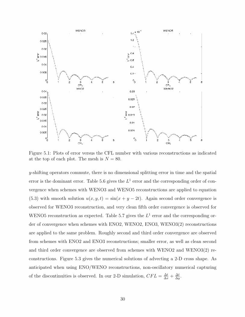
Figure 5.1: Plots of error versus the CFL number with various reconstructions as indicatedat the top of each plot. The mesh is N = 80.

y-shifting operators commute, there is no dimensional splitting error in time and the spatial

error is the dominant error. Table 5.6 gives the L1 error and the corresponding order of con-

vergence when schemes with WENO3 and WENO5 reconstructions are applied to equation

(5.3) with smooth solution u(x, y, t) = sin(x + y − 2t). Again second order convergence is

observed for WENO3 reconstruction, and very clean fifth order convergence is observed for

WENO5 reconstruction as expected. Table 5.7 gives the L1 error and the corresponding or-

der of convergence when schemes with ENO2, WENO2, ENO3, WENO3(2) reconstructions

are applied to the same problem. Roughly second and third order convergence are observed

from schemes with ENO2 and ENO3 reconstructions; smaller error, as well as clean second

and third order convergence are observed from schemes with WENO2 and WENO3(2) re-

constructions. Figure 5.3 gives the numerical solutions of advecting a 2-D cross shape. As

anticipated when using ENO/WENO reconstructions, non-oscillatory numerical capturing

of the discontinuities is observed. In our 2-D simulation, CFL = ∆t∆x

+ ∆t∆y

.

30

Table 5.3: First order scheme for (5.2) with u(x, t = 0) = 1 at T = 1 with CFL = 3.

– L1 error L∞ errormesh error order error order40 5.83E-2 – 0.17 –80 2.93E-2 0.99 8.80E-2 0.94160 1.47E-2 1.00 4.46E-2 0.98320 7.34E-3 1.00 2.23E-2 0.94640 3.67E-3 1.00 1.16E-2 1.00

Table 5.4: Schemes with ENO2 and WENO2 reconstructions for (5.2) with u(x, t = 0) = 1at T = 1 with CFL = 3.

– ENO2 WENO2– L1 error L∞ error L1 error L∞ error

mesh error order error order error order error order40 9.83E-3 – 8.98E-2 – 3.81E-3 – 2.47E-2 –80 3.99E-3 1.30 3.25E-2 1.47 9.20E-4 2.05 7.68E-3 1.69160 1.17E-3 1.77 2.10E-2 0.62 2.06E-4 2.16 1.95E-3 1.98320 5.38E-4 1.12 7.56E-3 1.48 4.77E-5 2.11 5.26E-4 1.89640 1.60E-4 1.75 2.08E-3 1.86 1.14E-5 2.06 1.42E-4 1.88

Example 5.4. (rigid body rotation)

ut − (yu)x + (xu)y = 0, x ∈ [−π, π], y ∈ [−π, π]. (5.4)

The equation is being Strang split into two one-dimensional equations, each of which is

evolved by the proposed semi-Lagrangian finite difference method. The initial condition we

used is plotted in Figure 5.4 in both mesh and contour plots. It includes a slotted disk,

a cone as well as a smooth hump, similar to the one in [19] for comparison purpose. The

numerical solutions after six full revolutions from schemes with WENO3, WENO5, ENO2,

WENO2, ENO3 and WENO3(2) reconstruction operators are plotted in Figure 5.5 by mesh

and in Figure 5.6 by slides benchmarked with exact solution. With all reconstructions,

non-oscillatory capturing of discontinuities is observed. However, schemes with high order

reconstruction, such as WENO5 and WENO3(2), are observed to be less dissipative, therefore

outperform schemes with lower order reconstructions.

31

Table 5.5: Schemes with ENO3 and WENO3 (2) reconstructions for (5.2) with u(x, t = 0) = 1at T = 1 with CFL = 3.

– ENO3 WENO3– L1 error L∞ error L1 error L∞ error

mesh error order error order error order error order40 2.26E-3 – 2.55E-2 – 4.61E-4 – 4.63E-3 –80 4.95E-4 2.19 6.41E-3 1.99 2.65E-5 4.12 5.82E-4 2.99160 9.28E-5 2.42 1.54E-3 2.05 1.27E-6 4.37 4.62E-5 3.66320 2.50E-5 1.89 4.28E-4 1.85 5.89E-8 4.44 3.08E-6 3.91640 4.25E-6 2.56 1.13E-4 1.92 4.13E-9 3.83 1.78E-7 4.11

Figure 5.2: Plots of error versus the CFL number with the mesh N = 80 and N = 160 forschemes with ENO2 (left) and WENO2 (right) reconstructions.

Example 5.5. (Swirling deformation flow) We use the test case in [19] with similar param-

eters to allow a direct comparison. We consider solving

ut − (cos2(x

2) sin(y)g(t)u)x + (sin(x) cos2(

y

2)g(t)u)y = 0, x ∈ [−π, π], y ∈ [−π, π], (5.5)

with g(t) = cos(πt/T )π. In our test case, we use the same set of initial condition as in

Example 5.4, which is quite challenging. We choose T = 1.5 and numerically integrate the

solution up to time 0.75, when the initial profile is greatly deformed, and to time 1.5, when

the initial profile is recovered. Figure 5.7 shows numerical results (in both mesh and con-

tour plots) from the scheme with ENO2 reconstruction with first order Strang splitting with

CFL = 2 and CFL = 1, and with second order Strang splitting with CFL = 1, when the

32

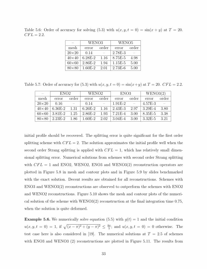
Table 5.6: Order of accuracy for solving (5.3) with u(x, y, t = 0) = sin(x + y) at T = 20.CFL = 2.2.

– WENO3 WENO5mesh error order error order20×20 0.14 – 2.78E-3 –40×40 6.28E-2 1.16 8.75E-5 4.9860×60 2.86E-2 1.94 1.15E-5 5.0080×80 1.60E-2 2.01 2.73E-6 5.00

Table 5.7: Order of accuracy for (5.3) with u(x, y, t = 0) = sin(x+y) at T = 20. CFL = 2.2.

– ENO2 WENO2 ENO3 WENO3(2)mesh error order error order error order error order20×20 0.16 – 0.14 – 1.91E-2 – 4.57E-3 –40×40 6.36E-2 1.31 6.26E-2 1.16 2.43E-3 2.97 3.29E-4 3.8060×60 3.81E-2 1.25 2.86E-2 1.93 7.21E-4 3.00 8.35E-5 3.3880×80 2.23E-2 1.86 1.60E-2 2.02 3.04E-4 3.00 3.32E-5 3.21

initial profile should be recovered. The splitting error is quite significant for the first order

splitting scheme with CFL = 2. The solution approximates the initial profile well when the

second order Strang splitting is applied with CFL = 1, which has relatively small dimen-

sional splitting error. Numerical solutions from schemes with second order Strang splitting

with CFL = 1 and ENO2, WENO2, ENO3 and WENO3(2) reconstruction operators are

plotted in Figure 5.8 in mesh and contour plots and in Figure 5.9 by slides benchmarked

with the exact solution. Decent results are obtained for all reconstructions. Schemes with

ENO3 and WENO3(2) reconstructions are observed to outperform the schemes with ENO2

and WENO2 reconstructions. Figure 5.10 shows the mesh and contour plots of the numeri-

cal solution of the scheme with WENO3(2) reconstruction at the final integration time 0.75,

when the solution is quite deformed.

Example 5.6. We numerically solve equation (5.5) with g(t) = 1 and the initial condition

u(x, y, t = 0) = 1, if√

(x− π)2 + (y − π)2 ≤ 8π5

; and u(x, y, t = 0) = 0 otherwise. The

test case here is also considered in [19]. The numerical solutions at T = 2.5 of schemes

with ENO3 and WENO3 (2) reconstructions are plotted in Figure 5.11. The results from

33

schemes with ENO3 and WENO3 (2) reconstructions approximate the exact solution quiet

well. They also outperform schemes with ENO2 and WENO2 reconstruction, whose plots

are omitted to save space.

6 Conclusions

In this paper, we propose a semi-Lagrangian finite difference scheme for simulating advection

in incompressible flows. Extensive numerical experiments, including the very challenging

problem of rigid body rotation and swirling deformation, have been performed by applying

the proposed semi-Lagrangian finite difference scheme with various reconstruction operators,

such as WENO3, WENO5, ENO2, WENO2, ENO3, WENO3 (2). The proposed high order

schemes have been shown to perform very well both by accuracy and by resolution of sharp

interface. Future research directions include (1) developing truly multi-dimensional semi-

Lagrangian finite difference scheme; (2) applications of algorithms developed in this paper

to relativistic plasma applications.

References

[1] M. Begue, A. Ghizzo, P. Bertrand, E. Sonnendrucker, and O. Coulaud,

Two-dimensional semi-Lagrangian Vlasov simulations of laser–plasma interaction in the

relativistic regime, Journal of Plasma Physics, 62 (1999), pp. 367–388.

[2] N. Besse and E. Sonnendrucker, Semi-Lagrangian schemes for the Vlasov equation

on an unstructured mesh of phase space, Journal of Computational Physics, 191 (2003),

pp. 341–376.

[3] J. Carrillo and F. Vecil, Nonoscillatory interpolation methods applied to Vlasov-

based models, SIAM Journal on Scientific Computing, 29 (2007), p. 1179.

[4] J. A. Carrillo, A. Majorana, and F. Vecil, A semi-lagrangian deterministic

solver for the semiconductor Boltzmann-Poisson system, Communications in Computa-

tional Physics, (2007), pp. 1027–1054.

34

[5] J. A. Carrillo and F. Vecil, Nonoscillatory Interpolation Methods Applied to

Vlasov-Based Models, SIAM Journal on Scientific Computing, 29 (2007), p. 1179.

[6] C. Cheng and G. Knorr, Integration of the Vlasov equation in configuration space,

tech. rep., COO–2059-47, Iowa Univ., Iowa City (USA). Dept. of Physics and Astron-

omy, 1975.

[7] P. Childs and K. Morton, Characteristic Galerkin methods for scalar conservation

laws in one dimension, SIAM Journal on Numerical Analysis, 27 (1990), pp. 553–594.

[8] A. Christlieb, M. Morton, and J.-M. Qiu, Higher order dimensional splitting

with integral deferred corrections with applications in Vlasov equation, In preparation.

[9] B. Cockburn, C. Johnson, C.-W. Shu, and E. Tadmor, Advanced numerical

approximation of nonlinear hyperbolic equations, Springer New York, 1998.

[10] P. Colella and P. Woodward, The piecewise parabolic method(PPM) for gas-

dynamical simulations, Journal of computational physics, 54 (1984), pp. 174–201.

[11] N. Crouseilles, G. Latu, and E. Sonnendrucker, Hermite spline interpolation

on patches for parallelly solving the Vlasov-Poisson equation, International Journal of

Applied Mathematics and Computer Science, 17 (2007), pp. 335–349.

[12] F. Filbet and E. Sonnendrucker, Comparison of eulerian Vlasov solvers, Com-

puter Physics Communications, 150 (2003), pp. 247–266.

[13] F. Filbet, E. Sonnendrucker, and P. Bertrand, Conservative numerical

schemes for the Vlasov equation, Journal of Computational Physics, 172 (2001), pp. 166–

187.

[14] S. Gottlieb, D. Ketcheson, and C. Shu, High order strong stability preserving

time discretizations, Journal of Scientific Computing, 38 (2009), pp. 251–289.

[15] A. Harten, B. Engquist, S. Osher, and S. Chakravarthy, Uniformly high

order essentially non-oscillatory schemes, III, Journal of Computational Physics, 71

(1987), pp. 231–303.

35

[16] F. Huot, A. Ghizzo, P. Bertrand, E. Sonnendrucker, and O. Coulaud,

Instability of the time splitting scheme for the one-dimensional and relativistic Vlasov–

Maxwell system, Journal of Computational Physics, 185 (2003), pp. 512–531.

[17] G.-S. Jiang and C.-W. Shu, Efficient implementation of weighted ENO schemes,

Journal of Computational Physics, 126 (1996), pp. 202–228.

[18] T. Lee and C. Lin, A characteristic Galerkin method for discrete Boltzmann equation,

Journal of Computational Physics, 171 (2001), pp. 336–356.

[19] R. LeVeque, High-resolution conservative algorithms for advection in incompressible

flow, SIAM Journal on Numerical Analysis, (1996), pp. 627–665.

[20] X.-D. Liu, S. Osher, and T. Chan, Weighted essentially non-oscillatory schemes,

Journal of Computational Physics, 115 (1994), pp. 200–212.

[21] J.-M. Qiu and A. Christlieb, A Conservative high order semi-Lagrangian WENO

method for the Vlasov Equation, Journal of Computational Physics, (accepted).

[22] J. Shi, C. Hu, and C. Shu, A technique of treating negative weights in WENO

schemes, Journal of Computational Physics, 175 (2002), pp. 108–127.

[23] C. Shu, High order weighted essentially non-oscillatory schemes for convection domi-

nated problems, SIAM Review, 51 (2009), pp. 82–126.

[24] C. Shu and S. Osher, Efficient implementation of essentially non-oscillatory shock-

capturing schemes, Journal of Computational Physics, 77 (1988), pp. 439–471.

[25] E. Sonnendrucker, J. Roche, P. Bertrand, and A. Ghizzo, The semi-

Lagrangian method for the numerical resolution of Vlasov equations.

[26] A. Staniforth and J. Cote, Semi-Lagrangian integration schemes for atmospheric

modelsA review, Monthly Weather Review, 119 (1991), pp. 2206–2223.

[27] H. Takewaki, A. Nishiguchi, and T. Yabe, Cubic interpolated pseudo-particle

method(CIP) for solving hyperbolic-type equations, Journal of Computational Physics,

61 (1985), pp. 261–268.

36

[28] T. Umeda, M. Ashour-Abdalla, and D. Schriver, Comparison of numerical

interpolation schemes for one-dimensional electrostatic Vlasov code, Journal of Plasma

Physics, 72 (2006), pp. 1057–1060.

37

Figure 5.3: Plots of the numerical solution of equation (5.3) with CFL = 2.2 at T = 1. Theinitial condition is a cross shape locating in the center of the domain. The numerical mesh is90×90. From left to right, from top to bottom are the solution from schemes with WENO3,WENO5, ENO2, WENO2, ENO3, WENO3(2) reconstructions.

38

Figure 5.4: Plots of the initial profile. The numerical mesh is 100× 100.

39

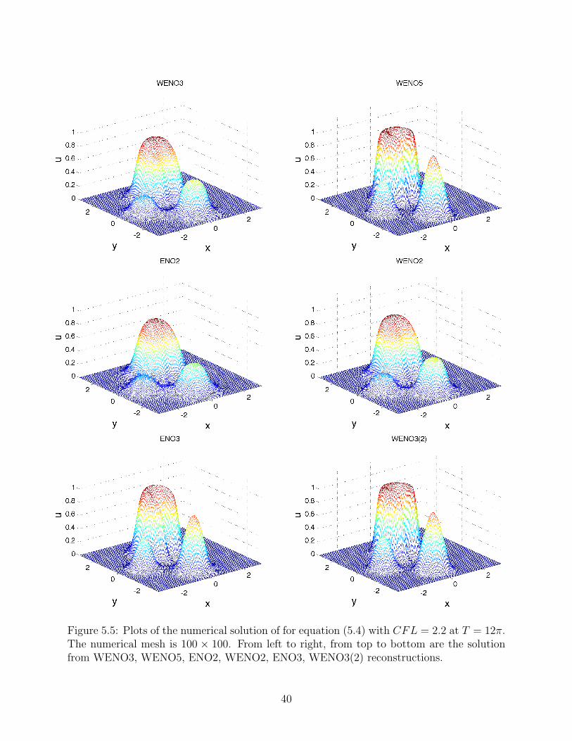
Figure 5.5: Plots of the numerical solution of for equation (5.4) with CFL = 2.2 at T = 12π.The numerical mesh is 100 × 100. From left to right, from top to bottom are the solutionfrom WENO3, WENO5, ENO2, WENO2, ENO3, WENO3(2) reconstructions.

40

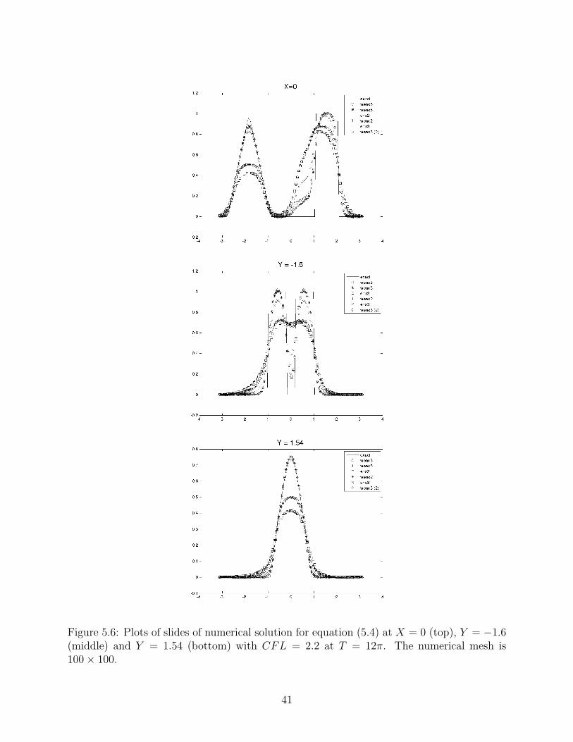
Figure 5.6: Plots of slides of numerical solution for equation (5.4) at X = 0 (top), Y = −1.6(middle) and Y = 1.54 (bottom) with CFL = 2.2 at T = 12π. The numerical mesh is100× 100.

41

Figure 5.7: Plots of the numerical solution of for equation (5.5) with first order splittingand CFL = 2 (top) and CFL = 1 (middle); and with second order splitting and CFL = 1(bottom). T = 1.5 and final integration time 1.5. The numerical mesh is 100× 100.

42

Figure 5.8: Plots of the numerical solution of schemes with second order splitting, CFL = 1and with different reconstruction operators as indicated at the top of each plot for equation(5.5). T = 1.5 and the final integration time 1.5. The numerical mesh is 100× 100.

43

Figure 5.9: Plots of slides of numerical solution for equation (5.5) benchmarked with exactsolution, at X = 0 (top), Y = −1.6 (middle) and Y = 1.54 (bottom) with second orderStrang splitting and CFL = 1. The numerical mesh is 100× 100.

44

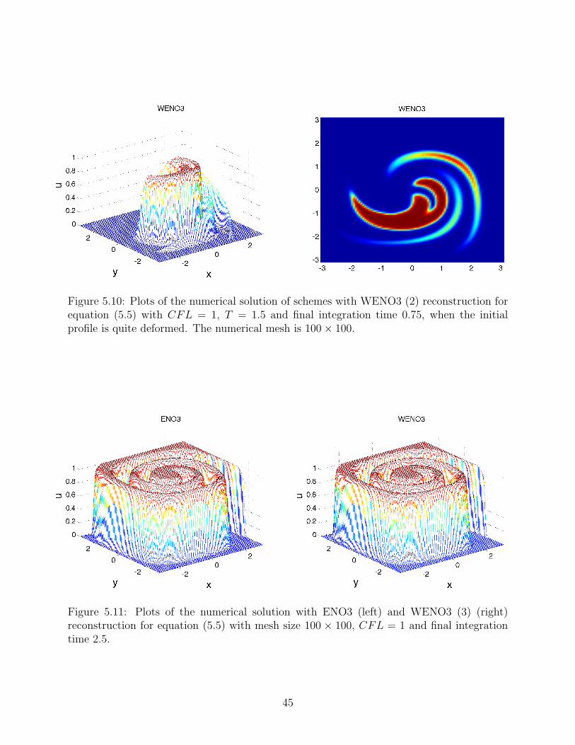
Figure 5.10: Plots of the numerical solution of schemes with WENO3 (2) reconstruction forequation (5.5) with CFL = 1, T = 1.5 and final integration time 0.75, when the initialprofile is quite deformed. The numerical mesh is 100× 100.

Figure 5.11: Plots of the numerical solution with ENO3 (left) and WENO3 (3) (right)reconstruction for equation (5.5) with mesh size 100 × 100, CFL = 1 and final integrationtime 2.5.

45