Abstract DNA-type systems

Diederik Aerts1 and Marek Czachor1,2

1 Centrum Leo Apostel (CLEA) and Foundations of the Exact Sciences (FUND)

Vrije Universiteit Brussel, 1050 Brussels, Belgium

2 Katedra Fizyki Teoretycznej i Metod Matematycznych

Politechnika Gdanska, 80-952 Gdansk, Poland

Abstract

An abstract DNA-type system is defined by a set of nonlinear kinetic equations with polynomial

nonlinearities that admit soliton solutions associated with helical geometry. The set of equations

allows for two different Lax representations: A von Neumann form and a Darboux-covariant Lax

pair. We explain why non-Kolmogorovian probability models occurring in soliton kinetics are

naturally associated with chemical reactions. The most general known characterization of soliton

kinetic equations is given and a class of explicit soliton solutions is discussed. Switching between

open and closed states is a generic behaviour of the helices. The effect does not crucially depend

on the order of nonlinearity (i.e. types of reactions), a fact that may explain why simplified models

possess properties occuring in realistic systems. We explain also why fluctuations based on Darboux

transformations will not destroy the dynamics but only switch between a finite number of helical

structures.

PACS numbers: 87.23.Cc, 03.67.Mn, 05.45.Yv

1

I. INTRODUCTION

There are certain aspects of the DNA dynamics that go far beyond standard fields of in-

terest of genetic engineering. A striking example is the observation that DNA is essentially a

universal Turing machine [1, 2]. The hardware of the machine consists of two strands (input-

output tapes) and an enzyme plays a role of finite control. As opposed to our PC’s that

cannot work without electricity, the DNA machine is powered by networks of autocatalytic

reactions. The double-helix structure is a trademark of the machine.

A new DNA helix is formed by a polymerase that moves along an existing strand and

gradually, step by step, produces the complementary strand. This seems to be a continuous

process that resembles the motion of finite control in a real-life Turing machine. The discrete

time-steps of an abstract Turing machine can be obtained if one looks at snapshots of the

evolution taken at times tn = n∆t, say. Finally, the two helices start to unwind, and the

two strands behave as the tapes of two new independent Turing machines. This process is

called replication.

The problem how to theoretically model the DNA dynamics is an old one. Between

various notable theoretical constructions one should mention classical Hamiltonian systems

(typically of a lattice type) [3–5] or replicator networks [7–9].

The above approaches are well motivated. There is little doubt that DNA is a nonlinear

dynamical system. It is also clear that the DNA evolution is a sequence of chemical reactions

and we know how to translate kinetic schemes into differential equations with polynomial

nonlinearities. Therefore no matter what networks of reactions one will invent, the result is

in general a set of nonlinear equations for certain nonnegative variables. As opposed to the

mechanical models, the kinetic equations are not directly linked to soliton systems.

The DNA dynamics does not look chaotic. One could even argue that organisms whose

DNA evolves in a chaotic way would be eliminated by natural selection. Systems that are

nonlinear and non-chaotic are almost certainly solitonic. Solitons are localized, propagate

in a stable way, and are very resistant to external noise. Soliton equations naturally lead

to ‘switches’, that is, solutions of a kink type. This is why, the line of research that deals

with Hamiltonian systems is concentrated on ‘DNA solitons’. Another argument in favour

of DNA solitons is that soliton scattering can serve as a model of computing [10–12]. The

DNA computer might be a soliton machine.

2

The latter observation points into another general class of dynamical systems: Those

whose discretized dynamics (in the sense of tn = n∆t snapshots) is equivalent to some

algorithm. The first example of such a link is the Toda lattice interpreted in terms of

spectrum generating algorithms [13]. Later on, the construction was generalized to a general

class of ‘Lax equations’ [14, 15]. The term ‘Lax equation’ is often applied to equations whose

right-hand side is given by a commutator. However, in the soliton case we need more than

just a commutator: We need a Darboux covariant Lax pair [16] and this is not exactly

synonymous to a commutator. Equations with commutator right-hand sides may not be

Darboux covariant. Or, even if they are Darboux covariant, the Darboux transformation

can be inconsistent with some important constraints.

To sum up, it looks like it would be ideal to work on DNA dynamics with soliton kinetic

equations that have some sort of Darboux-covariant Lax representation. Such equations do,

in fact, exist and can be characterized in quite general terms. To find them we are led by

still another hint: The ubiquity of helical structures associated with DNA dynamics. The

fact that the helices are formed (and deformed) as a result of the dynamics suggests their

3D parametrization of the form(

t, x(t), y(t))

, where t is time (i.e. position of the read/write

head) and x(t), y(t) are related to kinetic variables. The kinetic variables must therefore

occur in pairs. Alternatively, having an even number of dynamical variables one can always

work with their complex representation ξ(t) = x(t) + iy(t).

Let us now try to derive a simple kinetic scheme that leads to a helix. At this stage we

are satisfied by the ‘boring’ case of a helix that does not replicate. Consider the following

catalytic network [17]

Bk→ A+B (1)

A+Xk′→ X + (products) (2)

A +Bk→ A+ (products) (3)

Yk′′→ B (4)

Assume the reactions (2), (3) are 0-th order in A and B, respectively. Then

[A] = k[B]− k′[X], [B] = k′′[Y ]− k[A], [X] = [Y ] = 0. (5)

If we define two new (in general non-positive) variables x = [A] − (k′′/k)[Y ], y = [B] −(k′/k)[X], we can rewrite the system as iξ = kξ where ξ = x+ iy. The system evolves as a

3

harmonic oscillator. The curve t 7→ (t, [A(t)], [B(t)]) is a helix. If

H =

k 0

0 0

, ρ =

a ξ

ξ b

, (6)

a ≥ 0, b ≥ 0, a + b > 0, a = b = 0, then iρ = [H, ρ]. This is what we call a Lax form of the

kinetic equations. If eigenvalues of ρ are nonnegative at some t = t0 then for any projector PA

we have [A] = Tr ρPA ≥ 0. Let now PA and PB project, respectively, on

1

1

and

1

−i

.

Then x = [A]−(a+b)/2 and y = [B]−(a+b)/2, i.e. (k′/k)[X] = (k′′/k)[Y ] = (a+b)/2. The

kinetic variables satisfy [A(t)] = Tr ρ(t)PA and [B(t)] = Tr ρ(t)PB. The condition [B(t)] >

[A(t)] can be always satisfied by an appropriate shift of origin of the (x, y)-plane. What is

interesting, the projectors PA and PB do not commute (projectors in a plane commute if

and only if they project on either parallel or perpendicular directions, which is not the case

here). This type of noncommutativity is an indication of a non-Kolmogorovian probabilistic

structure behind the kinetics.

The above analysis explains the motivation for the formalism we develop in this paper.

We will work with kinetic equations that possess a two-fold Lax structure. First of all, all

these equations can be written as von Neumann type nonlinear systems. Secondly, each of

these equations can be regarded as a compatibility condition for a Darboux-covariant Lax

pair.

The Darboux transformation will also play a two-fold role in our formalism. It will allow

us to find nontrivial exact solutions of systems of coupled nonlinear kinetic equations. The

transformation is known to switch between different solutions of the equation in a way that

respects certain conservation laws (Casimir invariants). It is therefore also a natural formal

object representing fluctuations along a symplectic leaf of the dynamics. This effect will

lead to both mutation and formation of an open state in the associated helical structures.

That nonlinear von Neumann equations form a dynamical framework for various tradi-

tionally non-quantum domains was the main message we tried to convey in [18]. In the

present paper we lay special emphasis on the aspect that was implicitly present in all the

examples we gave, but which at a first glance may not be completely obvious: The fact

that von Neumann equations are not analogous but, in fact, exactly equivalent to systems of

kinetic equations. Any von Neumann equation is just a form of a Lax representation of a set

of kinetic equations (this observation was implicitly present also in the analysis of replicator

4

equations given in [19], although technically this argument was not equivalent to the one we

give below). This is why any integrable dynamical system that involves kinetic variables is

suspected of being implicitly von Neumannian.

In spite of its simplicity, the above statement is surprisingly difficult to digest by the

community of chemists or molecular biologists. The roots of the difficulty seem to be related

to the misleading term ‘quantum probability’ suggesting that non-commutative propositions

are restricted only to microscopic systems.

Therefore, one element we will need to understand before launching on technicalities

of soliton kinetic equations, is the structure of probability models that are behind soliton

kinetic evolutions. We have seen already at the simple example discussed above, that the

‘concentrations’ [A] and [B] were linked to noncommuting projectors PA and PB. This type of

noncommutativity is a typical feature of soliton kinetics and indicates that the probability

calculus is here nonclassical. We therefore need to clarify some formal aspects of non-

Kolmogorovian probability, and explain why this is the type of formalism that necessarily

occurs in chemical kinetics.

II. HILBERTIAN MODEL OF PROBABILITY

A proposition is represented by a self-adjoint operator with eigenvalues 0 and 1, i.e. a

projector P = P † = P 2 acting in a Hilbert space H. Probability is computed by means of

the formula

p = TrPρ (7)

where ρ is a ‘density operator’ (‘density matrix’) acting also in H and satisfying ρ = ρ†

(since then probabilities are real: TrPρ = TrPρ = TrPρ†), ρ > 0 (i.e. the eigenvalues of

ρ are non-negative) since then p ≥ 0. The normalization of probability leads to Tr ρ = 1: If

the set {Pj} of orthogonal projectors is complete in the sense that∑

j Pj = 1 then

∑

j

pj = 1 =∑

j

TrPjρ = Tr ρ. (8)

In a given Hilbert space there exists an infinite number of such complete sets. If a given prob-

lem can be represented entirely in terms of probabilities associated with a single complete

set, then all the probabilities will satisfy criteria typical of Kolmogorovian models.

5

If the kinetics is implicitly Hilbertian then all the dynamical variables, say p1, p2, . . . , pN ,

have to allow for a representation of the form (7). If a given set of kinetic equations couples

probabilities p1, . . . , pN that do not belong to the same complete set then∑N

j=1 pj 6= 1. This

happens whenever the set {Pj} involves projectors that do not commute with one another

since then necessarily∑

j Pj 6= 1. Actually, this is what we found in the simple kinetic model

of harmonic oscillators discussed in the Introduction, where PA and PB did not commute

and, hence, did not belong to the same maximal set.

It follows that the conditions we impose on the kinetic equations can be reduced to the

requirements imposed on the dynamics of the density operator ρ(t): For all times t1 < t < t2

in the interval of interest we must find (i) ρ(t) = ρ(t)†, (ii) ρ(t) > 0, and Tr ρ(t) = const <∞.

A basis in the Hilbert space is given by a set {|n〉, 〈n|m〉 = δnm}. Matrix elements of the

density operator are in general complex

ρnm = 〈n|ρ|m〉 = xnm + iynm (9)

ρnm = xnm − iynm = xmn + iymn = ρmn (10)

and thus xmn = xnm, ymn = −ynm, ynn = 0.

The diagonal elements ρnn = xnn are themselves probabilities since

ρnn = 〈n|ρ|n〉 = TrPnρ = pn = xnn (11)

where Pn = |n〉〈n|. Now, let

|jk〉 =1√2

(

|j〉+ |k〉)

, |jk′〉 =1√2

(

|j〉 − i|k〉)

, (12)

Pjk = |jk〉〈jk|, P ′jk = |jk′〉〈jk′|. Then

xjk = pjk −1

2pj −

1

2pk, (13)

yjk = p′jk −1

2pj −

1

2pk, (14)

ρjk = pjk + ip′jk −eiπ/4

√2

(pj + pk), (15)

where pjk = TrPjkρ, p′jk = TrP ′jkρ. It follows that a single density operator ρ encodes three

families of probabilities: {pn}, {pjk}, and {p′jk}. They are associated with three families of

projectors: {Pn}, {Pjk}, and {P ′jk}. Additional relations between the probabilities follow

from

xjj = pj = pjj − pj, yjj = 0 = p′jj − pj (16)

6

and the resulting formula pj = p′jj = pjj/2. Let us note that {Pn} is complete, i.e.∑dimH

n=1 Pn = 1,∑dimH

n=1 pn = 1. In order to understand completness properties of {Pjk}and {P ′

jk} we introduce, for j < k, two additional types of vectors and their associated

projectors:

|jk⊥〉 =1√2

(

|j〉 − |k〉)

, |jk′⊥〉 =1√2

(

|j〉+ i|k〉)

, (17)

P⊥jk = |jk⊥〉〈jk⊥|, P ′

jk⊥ = |jk′⊥〉〈jk′⊥|. The completeness relations for {Pjk} and {P ′

jk}follow from the formula

Pjk + P⊥jk = Pj + Pk = P ′

jk + P ′jk⊥. (18)

The non-Kolmogorovity of the set of probabilities can be illustrated by means of uncer-

tainty relations. Indeed, for any three operators satisfying [A,B] = iC one can prove the

uncertainty relation ∆A∆B ≥ 12|〈C〉| where ∆A =

√

〈A2〉 − 〈A〉2, 〈A〉 = Tr (Aρ), etc.

If A = P = P 2 is a one-dimensional projector then 〈P 〉 = p is a probability and one

finds ∆P =√

p(1− p). We say that two propositions P1 and P2 are complementary if

∆P1∆P2 ≥ ε > 0.

In order to show that the propositions, say Pj and Pjk, are complementary, we compute

[Pj, Pjk] = 12

(

|j〉〈k| − |k〉〈j|)

= iC (19)

and 〈C〉 = ykj. Finally,

√

pj(1− pj)√

pjk(1− pjk) ≥ 12|ykj|. (20)

The variable ykj measures complementarity of Pj and Pjk.

In supersymmetric projector model we start with γ : H → H and define the ‘supercharge’

Q : H⊕H → H⊕H,

Q =

0 γ

γ† 0

, Q2 =

γγ† 0

0 γ†γ

, ρ =Q2

Tr (Q2)(21)

The situation where there are two types of super-partner density matrices is encountered in

semantic analysis [20]. In semantic contexts the two density matrices correspond to words

and sentences, respectively, and it is an intriguing issue if a link to DNA is here accidental.

We use the model to describe the process of unwinding of two helices.

7

Any of the probabilities we have discussed above is consistent with the frequency inter-

pretation of experiments since always 0 ≤ p ≤ 1. The subleties related to different models

become visible when one comes to joint and conditional probabilities, since only with at

least two propositions the issues of non-commutativity become relevant.

The act of conditioning by a positive answer to the question represented by a projector

P changes density matrices according to

ρ 7→ ρ1 =PρP

Tr (PρP ). (22)

Joint probability of successes in a sequence of measurements P1, P2, . . . , Pk reads

p(P1 ∩ · · · ∩ Pk) = Tr (P1 . . . Pk−1PkPk−1 . . . P1ρ).

Here P1 is the first measurement and Pk — the last. Since projectors belonging to differ-

ent maximal sets do not all commute with one another, the joint probabilities have to be

associated with noncommutativity of some sort. In molecular context the most natural non-

commutativity is associated with chemical reactions: It is typical that the reactions X → Y

and Y → X involve different kinetic constants. In particular, it is possible that the chain

X → Y → Z of elementary reactions is possible, whereas the direct reaction X → Z is not

allowed. One can see here an analogy to the well known Malusian experiment with photons

and three polarizers. It is worth mentioning that the very fact that some diagrams of the

form X → Y are not allowed may imply a Hilbert space structure [21], of course under some

asumptions about the dynamics.

III. SOLITON KINETIC EQUATIONS

Let us characterize soliton kinetic equations in a general way. In explicit examples we

will work only with a particular case, but since the subject is not widely known we find it

important to set our results in a more general context. For further technicalities the readers

are referred to [22, 23]. Consider an operator-valued function

Xλ =

L∑

n=0

λnX(n) +

M∑

n=1

λ−nX(−n) (23)

of a complex spectral parameter λ. An invertible operator Dλ is a Darboux matrix for Xλ if

Xλ[1] = D−1λ XλDλ =

L∑

n=0

λnX(n)[1] +

M∑

n=1

λ−nX(−n)[1] (24)

8

where the X(n)[1], X(−n)[1] are λ-independent [24–29]. In this paper we work with

Dλ = 1 +ν − µ

µ− λP (25)

where P = P 2 is a projector constructed in terms of right and left eigenvectors of, respec-

tively, Xµ and Xν [30–34]. If ν = µ and P = P † then Dλ is unitary: D−1λ = D†

λ. Of

particular importance is the case

X(λ) =L

∑

n=0

λnXn (26)

since then putting λ = 0 in (26) we obtain

X(0)[1] = X0[1] = D−10 X0D0 = D−1

0 X(0)D0. (27)

In later applications to kinetic equations we will work with unitary Dλ and X0 = ρ.

Now consider two operator-valued functions F (X) and G(X) restricted only by

[F (X), X] = [G(X), X] = 0, (28)

F (TXT−1) = TF (X)T−1, (29)

G(TXT−1) = TG(X)T−1, (30)

for any T . The Lax pair is

zλψλ = ψλX(λ), −iψλ = ψλY(λ) (31)

where zλ are complex numbers, and

X(λ) =

N∑

k=0

λkXk, (32)

Y(λ) =L

∑

k=0

λkAk +M

∑

k=1

1

λkBk = Y(λ)(X0, . . . , XN), (33)

Ak =1

(L− k)!

(

dL−k

dςL−kF

(

ςNX(ς−1)

)

)∣

∣

∣

∣

ς=0

(34)

Bk =1

(M − k)!

(

dM−k

dεM−kG

(

X(ε)

)

)∣

∣

∣

∣

ε=0

(35)

The compatibility condition for the Lax pair consists on N + 1 equations

iXm =

N∑

k=m+1

[Xk, Am−k] +

m∑

k=0

[Xk, Bk−m], 0 ≤ m ≤ N. (36)

9

For k < 0 the operators are defined by means of (34) and (35). The equation for m = 0 is

the von Neumann equation in question, and those for m > 0 are additional relations between

other operators occuring in the von Neumann equation.

The Darboux matrix defines a Darboux transformation for the Lax pair and its compat-

ibility conditions as follows. Take X(n)[1] defined via (24), and Ak[1], Bk[1] defined by (34),

(35), but with X(n) replaced by X(n)[1]. Then

iXm[1] =N

∑

k=m+1

[Xk[1], Am−k[1]] +m

∑

k=0

[Xk[1], Bk−m[1]], 0 ≤ m ≤ N, (37)

and

zλψλ[1] = ψλ[1]X(λ)[1], −iψλ[1] = ψλ[1]Y(λ)[1] (38)

with ψλ[1] = ψλDλ. Restricting the operators Xm to matrices and defining for X0 = ρ =

ρ† > 0 the kinetic variables according to the recipes of Sec. II we arrive at systems of soliton

kinetic equations.

IV. ONE-FIELD EQUATIONS

We now restrict the explicit examples to ‘one-field’ equations, that is, those corresponding

to N = 1, i.e.

X(λ) = X0 + λX1 = ρ+ λH. (39)

The equations are one-field since only X0 = ρ depends on time. One of the two dynamical

equations reads here X1 = 0. Examples of N > 1 equations can be found in [22, 23]. An

interesing class of nonlinearities occurs for F (X) = 0, M = 1, G(X) = −f(X). Then

iρ = [H, f(ρ)]. (40)

The right-hand-side of (40) can be rewritten as [Hf(ρ), ρ], with Hf (ρ) whose explicit form

depends on f , showing that this is indeed a von Neumann equation. The equation itself

was introduced in [35] and later discussed in the context of non-extensive statistics in [36].

The soliton technique of integration based on Darboux-covariant Lax representation was

introduced in [37] and a class of 1-soliton self-switching solutions was there found for f(ρ) =

ρ2. The Lax-pair representation and Darboux covariance properties of the general form were

10

established in [38] and explicit self-switching solutions were there found for f(ρ) = ρq−2ρq−1,

where q is an arbitrary real number. The explicit form of the Lax pair is simple

iψλ =1

λψλf(ρ), zλψλ = ψλ(ρ+ λH). (41)

In the context of autocatalytic networks the examples of interest involve third order polyno-

mial nonlinearities: f(ρ) = a3ρ3 + a2ρ

2 + a1ρ. Let us choose f(ρ) = ρ3 − 2ρ2. The equation

can be written in two equivalent forms

iρ = [H, ρ3 − 2ρ2] = [H(ρ), ρ], (42)

H(ρ) = ρ2H + ρHρ+Hρ2 − 2(Hρ+ ρH) (43)

Taking

H =

0 0 0

0 k 0

0 0 2k

(44)

and performing the splitting (15) we obtain six coupled kinetic equations with nonlinearities

of third order. A closer look at their structure reveals that the reduction of variables from

six to four can be obtained if one imposes the constraint

ρ23 = zρ12, ρ32 = zρ21, ρ11 = ρ33, |z| = 1. (45)

Assuming the above reduction with z = −1 and introducing the four variables,

A = [A]− 1

2p1 −

1

2p2 = x12 (46)

B = [B]− p1 = x13 (47)

C = [C]− 1

2p1 −

1

2p2 = y12 (48)

D = [D]− p1 = y13, (49)

where xij and yij are, respectively, real and imaginary parts of ρij, [A], [B], [C], [D], are

nonnegative for all times and p1 = ρ11, p2 = ρ22 are constants, we can rewrite the von

Neumann equation as the set of four kinetic equations

11

[A] = −k(

2C3 + 2A2C − AD(2p1 + p2 − 2)

+ C(

B2 +D2 − 2p1 + p21 − 2p2 + p1p2 + p2

2 +B(2p1 + p2 − 2))

)

(50)

[B] = −2k(

D3 + 2A2D +D(B2 + 2C2 − 4p1 + 3p21)− 2AC(2p1 + p2 − 2)

)

(51)

[C] = k(

2A3 − CD(2p1 + p2 − 2)

+ A(

B2 + 2C2 +D2 − 2p1 + p21 − 2p2 + p1p2 + p2

2 − B(2p1 + p2 − 2))

)

(52)

[D] = 2k(

B3 +B(

2C2 +D2 + p1(−4 + 3p1))

+ A2(2 + 2B − 2p1 − p2) + C2(2p1 + p2 − 2))

(53)

It is possible to derive this system of kinetic equations from a system of elementary reactions

of order not higher than three. This system of equations is a particular case, for q = 3, of

the general equation iρ = [H, ρq − 2ρq−1]. Its solution for an arbitrary value of q, found in

[38] by means of Darboux transformations, reads

ρ =

3/2 −ξ(t) ζ(t)

−ξ(t) 7/4 ξ(t)

ζ(t) ξ(t) 3/2

, (54)

ξ(t) =(−3i +

√3)eωq(t−t0)

4√

2(

1 + e2ωq(t−t0)) eikt, (55)

ζ(t) =1− i

√3− 2e2ωq(t−t0)

4(

1 + e2ωq(t−t0)) e2ikt, (56)

ωq = [(4/7)1−q − 1]k/√

3. This solution is not normalized and hence the kinetic variables

have be to rescaled if one is interested in probablities: pA = [A]/Tr ρ, and so on. Properties

of the solution are illustrated by the figures. The scale of simplification and the efficiency of

the von Neumann formalism become evident if one compares the von Neumann and kinetic

forms of the same dynamics.

V. FLUCTUATIONS VIA DARBOUX TRANSFORMATIONS

The set of solutions of von Neumannn kinetic equations is naturally equipped with the

Hilbert-Schmidt norm. The distance between two solutions ρ(t) and ρ(t) is

‖ ρ(t)− ρ(t) ‖=√

Tr(

ρ(t)− ρ(t))2. (57)

12

The solutions (54) describe families of distorted helices. We will now explicitly show that for

any distorted helix (54)–(56) there exist two families of undeformed helices corresponding

to two different solutions ρ±(t) of the same equation, such that (i) eigenvalues of ρ(t), ρ+(t),

and ρ−(t) are identical, (ii) ρ(t) and ρ±(t) are linked by Darboux transformations, (iii) ρ(t)

and ρ±(t) belong to the same symplectic leaf of the Lie-Poisson structure corresponding to

the dynamics (i.e. their Poisson-reduced dynamics occurs in the same phase-space), and (iv)

‖ ρ(t)− ρ±(t) ‖< ε (58)

for any ε > 0 and for an infinitely long period of time t. In other words, an arbitrarily

long part of an undeformed helix is arbitrarily close to a helix that involves a defect. In

principle, a small fluctuation of the undeformed helix, at some t and along a symplectic

leaf of the dynamics, may map it into a helix with a defect. However, if one restricts the

analysis to a finite-length helix t1 < t < t2 (corresponding to a finite number of steps

tn = n∆t), then the defect may or may not become visible, because different Darboux-

transformation fluctuations of the same ρ(t) result in helices with different locations of the

defect (parametrized by t0). How quickly will the defect occur depends on what kind of

a Darboux transformation is responsible for the fluctuation ρ(t) 7→ ρ(t). To see how this

works consider

ρ±(t) =

3/2 0 ζ±(t)

0 7/4 0

ζ±(t) 0 3/2

, ζ+(t) = −1

2e2ikt, ζ−(t) =

1− i√

3

4e2ikt. (59)

Density matrices ρ±(t) are the asymptotic forms of ρ(t) for −ωqt0 → ±∞. These two q-

independent asyptotes also satisfy iρ± = [H, ρq± − 2ρq−1

± ] for any real q, which follows from

the fact that they can be obtained from the same solution by Darboux transformations

differing by initial conditions for the Lax pair. This immediately implies that all these

density matrices are isospectral and possess the same values of the Casimirs Tr (ρn). The

Casimirs allow to reduce the Lie-Poisson structure to the same symplectic leaf, and thus

the fluctuations occur in the same phase-space. The corresponding Hamiltonian function is

given by TrHf(ρ).

13

VI. FORMATION OF OPEN STATE IN THE SUPERSYMMETRIC MODEL

The supersymmetric model naturally leads to the double-helix structure. Consider an

arbitrary operator γ whose relation to a density matrix is ρ = γ†γ. A superpartner of ρ is

defined in the usual way as ρ = γγ†. This type of structue is encountered in Latent Semantic

Analysis where ρ and ρ represent word-vector and sentence-vector density matrices [20].

We know that the Darboux transformation acts on density matrices by ρ 7→ ρ1 = D†0ρD0.

This is equivalent to γ 7→ γ1 = γD0, if ρ1 = γ†1γ1, or the supercharge transformation

Q 7→

1 0

0 D†0

0 γ

γ† 0

1 0

0 D0

=

0 γ1

γ†1 0

= Q1,

where Q is given by (21). The action of the Darboux transformation on the super-density

matrix is

Q21 =

γ1γ†1 0

0 γ†1γ1

=

γγ† 0

0 D†0γ

†γD0

=

ρ 0

0 ρ1

(60)

since D0 is unitary. At the level of super-density matrices the Darboux transformation acts

by

ρ 0

0 ρ

7→

ρ 0

0 ρ1

. (61)

Of particular interest is the symmetric case γγ† = γ†γ. This is trivially satisfied if γ = γ†

and γ itself is a supercharge for ρ = ρ. Such a γ always exists since ρ, being a positive

operator, possesses a unique square root√ρ = γ. The Darboux transformation breakes this

symmetry as follows

ρ 0

0 ρ

7→

ρ 0

0 ρ1

. (62)

It is interesting that any sequence of Darboux transformations is here necessarily cyclic in

the sense that

ρ 0

0 ρ

→

ρ 0

0 ρ1

→ · · · →

ρ 0

0 ρn

→

ρ 0

0 ρ

with n being related to the dimension of the matrix ρ. To understand why this has to

happen let us recall that the Darboux transformation involves two solutions of a Lax pair:

14

The one that is transformed, and the one that is used to define the transformation. The

transformation is trivial if the two solutions are linearly dependent. It is clear that the

number of linearly independent solutions is limited by the dimension of the linear space

they live in. In the context of 3× 3 solutions we find

ρ→ ρ1 → ρ2 → ρ3 → ρ, (63)

no matter what (nontrivial) transformations have been performed, and two of these four

density matrices have the asymptotic form ρ±(t). This is why after four Darboux fluctuations

the system returns to its original state.

For super-density matrices this process is strikingly similar to what happens with DNA

during formation of an open state. Initially we have two identical strands described by the

symmetric state ρ = ρ. The first nontrivial fluctuation maps it into the pair (ρ, ρ1) whose

evolution looks as either Fig. 1 or Fig. 2 where ρ and ρ1 correspond to the two helices. Let

us note, that the helices are practically overlapping over arbitrarily long parts, and therefore

an arbitrarily small fluctuation may turn one into another. If the fluctuation is of the form

shown in Fig. 1 then somewhere in the future the two helices will unwind, unless a new

fluctuation will prevent it. If the fluctuation is of the form shown in Fig. 2, then the helix

switches into a helix that wants to return to the asymptote, and we will not see a change of

form. However, if the helices disentangled, then the helix approaches the other asymptote,

and a subsequent small fluctuation will not be observed. Finally, another fluctuation maps

it into a state that starts to return asymptotically to the original state.

The fluctuations deform the helices according to the scheme (63). However, we do not

know which Darboux transformation is responsible for ρ → ρ1, say. The point is that this

is not really important! Fig. 5 shows two helices corresponding to two randomly chosen

Darboux transformations. The random element is when do the helices start to unwind.

All these helices have the same asymptotic forms and the part where the two helices look

different is the one where the Hilbert-Schmidt distance is maximal.

One can illustrate this phenomenon if one plots the Hilbert-Schmidt distance between

two helices whose forms differ by the parameter t0. The fluctuation via a Darboux trans-

formation is essentially equivalent to the fuctuation of the parameter α that occurs in the

transformation. Fig. 6 shows the plot of the Hilbert-Schmidt distance between two solutions

that were produced from the same seed solution by two different Darboux transformations,

15

as a function of t and the fluctuation parameter t0 (in one solution t0 = 0 and is arbitrary

in the other one). Two such density matrices effectively differ from each other in a finite

time interval.

VII. SUMMARY AND PERSPECTIVES

We have started with the observation that a system evolving into helical structures has to

resemble an oscillator, at least at a sufficiently abstract level of description. Armed with this

intuition and the fact that dynamical equations of DNA must be kinetic in some sense we

have arrived at equations of a von Neumann type. Then, imposing soliton-type integrability,

we restricted the class to Darboux-covariant von Neumann equations.

The formalism we have proposed has many possible continuations. We have touched only

the tip of the iceberg. Even the one-field equations are more general than those with the

right-hand side [H, f(ρ)]. As shown in [23], the class contains also Toda and other integrable

lattices as particular cases. Solutions can be found by the same Darboux transformation, but

one has to employ a different explicit technique of finding nontrivial seed solutions (cf. [40]).

Still another technique of finding appropriate seed solutions that generalizes to arbitrary

H and f(ρ) the method we have worked with, was introduced in [41]. When applied to

explicit matrix examples the method leads again to qualitatively the same solutions as those

we already know. One can risk the statement that the type of behavior (unwinding and

switching between a finite number of states) we have described is generic for the whole class

of integrable kinetic equations. In the context of genericity one should mention also the

stability of solutions for f(ρ) = ρq − 2ρq−1 under modifications of q (cf. the discussion in

[38]). This means that the behaviour of the helix is basically the same for q = 3 and, say,

q = 1000, or a non-integer q. If one tried to write down kinetic equations corresponding

to q = 1000 one would have found the set of equations with polynomials of order 1000 and

thousands of terms. Analogously, there would have been thousands of elementary very-high

order reactions that, effectively lead to almost identical replication and unwinding as q = 3

or q = 2. This fact may explain why incredibely simplified kinetic schemes one employs

in replication retworks lead to evolutions that reasonably approximate various effects one

expects in DNA-type systems.

16

pp’

t

p’

FIG. 1: Formation of open state. The red, black, blue, and green helices represent, respectively,

the matrix elements ρ−(t)13, ρ(t)13, ρ−(t)12, and ρ(t)12. ρ(t) and ρ−(t) are given by (54) and

(59). The helices practically overlap in the past and unwind in a neighbourhood of t = 0. The

four helices behave as if the external ones were the tapes, and the internal ones represented the

read/write head.

Acknowledgments

The work of MC is a part of the Polish Ministry of Scientific Research and Information

Technology (solicited) project PZB-MIN 008/P03/2003. We acknowledge the support of

the Flemish Fund for Scientific Research (FWO Project No. G.0335.02). MC is grateful to

professor Stanis law Koter for his comments on chemical harmonic oscillations.

[1] C. H. Bennett, R. Landauer, Scientific American 253, 48-56 (1985).

[2] L. M. Adleman, Science 266, 1021 (1994).

[3] S. W. Englander et al., Proc. Nat. Acad, Sci. 77, 7222 (1980).

[4] L. V. Yakushevich, Nonlinear Physics of DNA (Wiley, New York, 1998).

[5] L. V. Yakushevich, J. Biosci. 26, 305 (2001).

[6] B. Hartmann, W. J. Zakrzewski, J. Nonlin. Math. Phys. 12 (2005) — in print.

17

pp’

t

p’

FIG. 2: Formation of closed state. The red, black, blue, and green helices represent, respectively,

the matrix elements ρ+(t)13, ρ(t)13, ρ+(t)12, and ρ(t)12. ρ(t) and ρ+(t) are given by (54) and (59).

The helices practically overlap in the future and get wound up in a neighbourhood of t = 0.

1.2 1.4 1.6 1.8 2p

1.2

1.4

1.6

1.8

2

p’

FIG. 3: Projection of Fig. 1 and Fig. 2 on the (p, p′)-plane.

[7] M. Eigen, Natuwissenschaften 58, 465 (1971).

[8] P. Schuster and K. Sigmund, J. Theor. Biol. 100, 533 (1983).

[9] J. Hofbauer and K. Sigmund, Dynamical Systems and the Theory of Evolution (Cambridge

18

-10 -5 5 10t

0.2

0.4

0.6

0.8

1

1.2

Hilbert-Schmidt distance

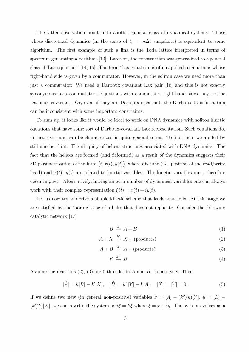
FIG. 4: Hilbert-Schmidt distances ‖ ρ(t)−ρ+(t) ‖ (dotted), and ‖ ρ(t)−ρ−(t) ‖ (full) as functions

of time. ρ(t) and ρ±(t) are given by (54) and (59).

p

p’

t

p’

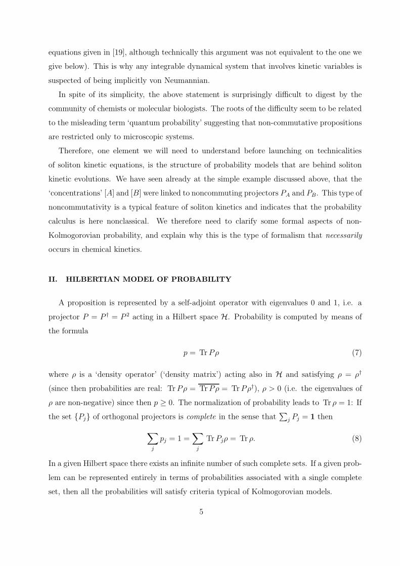
FIG. 5: Two helices obtained from the same ρ by means of two nontrivial Darboux transformations.

The distance between two such helices is shown in the next figure.

University Press, Cambridge, 1988).

[10] K. Steiglitz, I. Kamal, and A. H. Watson, IEEE Transactions on Computers 37, 138 (1988).

[11] M. H. Jakubowski, K. Steiglitz, and R. K. Squier, Complex Systems 10, 1 (1996).

[12] M. H. Jakubowski, K. Steiglitz, and R. K. Squier, Phys. Rev. E 58, 6752 (1998); Phys. Rev.

19

-20-10

0

10

20

t-10

-5

0

5

10

t0

0

0.5

1

-20-10

0

10

20

t

FIG. 6: Hilbert-Schmidt distance between two solutions corresponding, respectively, to t0 = 0 and

an arbitrary t0, plotted as a function of time t and the parameter t0. Solutions differing by different

values of t0 are obtained from the same seed solution by two different Darboux transformations.

The distance is maximal in the part of the plot where the two corresponding helices are unwound

(the ‘open state’).

E 56, 7267 (1997)

[13] W. Symes, Physica D 4, 275 (1982).

[14] M. Przybylska, Linear Algebra Appl. 346, 155 (2002).

[15] M. Przybylska, Future Generation Comp. Syst. 19, 1165 (2003).

[16] V.B. Matveev, M.A. Salle, Darboux Transformations and Solitons (Springer–Verlag, Berlin–

Heidelberg, 1991).

[17] S. Koter, private communication.

[18] D. Aerts, M. Czachor, L. Gabora, M. Kuna, A. Posiewnik, J. Pykacz, and M. Syty, Phys. Rev.

E 67, 051926 (2003).

[19] V. V. Gafiychuk and A. K. Prykarpatsky, J. Nonlin. Math. Phys. 11, 350 (2004).

[20] D. Aerts and M. Czachor, J. Phys. A: Math. Gen. 37, L123 (2004).

[21] D. R. Finkelstein, Quantum Relativity: A Synthesis of the Ideas of Einstein and Heisenberg

(Springer, Berlin, 1996).

[22] N. V. Ustinov and M. Czachor, in Probing the Structure of Quantum Mechanics: Nonlinearity,

Nonlocality, Computation, and Axiomatics, Eds. D. Aerts, M. Czachor, and T. Durt (World

20

Scientific, Singapore, 2002), 335.

[23] J. L. Cieslinski, M. Czachor, and N. V. Ustinov, J. Math. Phys. 44, 1763 (2003).

[24] V. E. Zakharov and A. B. Shabat, Funk. Anal. Pril. 13, 13 (1979) (in Russian).

[25] S.P. Novikov, S.V. Manakov, L.P. Pitaevski and V.E. Zakharov, Theory of Solitons, the Inverse

Scattering Method (Consultants Bureau, New York, 1984).

[26] D. Levi, O.Ragnisco, and M. Bruschi, Nuovo Cim. 58A, 56 (1980).

[27] A.V. Mikhailov, Physica D3, 73 (1981).

[28] G. Neugebauer and D. Kramer, J. Phys. A: Math. Gen. 16, 1927 (1983).

[29] J. L.Cieslinski, J. Math. Phys. 32, 2395 (1991); ibid. 36, 5670 (1995).

[30] S.B. Leble and N.V. Ustinov, Solitons of nonlinear equations associated with degenerate spec-

tral problem of the third order, in: Nonlinear Theory and its Applications, Eds. M. Tanaka

and T. Saito (World Scientific, Singapore, 1993) v.2, pp.547-550.

[31] N. V. Ustinov, J. Math. Phys. 39, 976 (1998).

[32] S. B. Leble, Computers Math. Applic. 35, 73 (1998).

[33] J. L. Cieslinski, J. Phys. A: Math. Gen. 33, L363 (2000).

[34] W. Biernacki and J. L. Cieslinski, Phys. Lett. A 288, 167 (2001).

[35] M. Czachor, Phys. Lett. 225A, 1 (1997).

[36] M. Czachor and J.Naudts, Phys. Rev. 59E, R2497 (1999).

[37] S.B. Leble and M. Czachor, Phys. Rev. 58E, 7091 (1998).

[38] N.V. Ustinov, M. Czachor, M. Kuna, and S.B. Leble, Phys. Lett. A 279, 333 (2001).

[39] The solutions were checked by means of Mathematica 4.2.

[40] M. Kuna, M.Czachor and S.B. Leble, Phys. Lett. 255A, 42 (1999).

[41] M. Kuna, quant-ph/0408048.

21