abstract - inspire hepinspirehep.net/record/1358293/files/kozlov.pdf · ingo ald, ew jan h riedric...

High-Resolution Study of the

4

He(e; e

0

p) Reaction in

the Quasielastic Region

Alexander A. Kozlov

M.Sc., Kharkov State University (1992)

Submitted in total fullment of the requirements of the degree of

Doctor of Philosophy

School of Physics

The University of Melbourne

Victoria 3010

Australia

June 10, 2000

Abstract

A high-resolution study of the (e; e

0

p) reaction on

4

He was carried out at the Institut

fur Kernphysik in Mainz, Germany. The high quality 100 % duty factor electron

beam, and the high-resolution three-spectrometer-system of the A1 collaboration

were used. The measurements were done in parallel kinematics at a central mo-

mentum transfer j~qj = 685 MeV/c, and at a central energy transfer ! = 334 MeV,

corresponding to a value of the y-scaling variable of +140 MeV/c. In order to enable

the Rosenbluth separation of the longitudinal

L

and transverse

T

response func-

tions (as dened in [13]), three measurements at dierent incident beam energies,

corresponding to three values of the virtual photon polarization , were performed.

The absolute (e; e

0

p) cross section for

4

He was obtained as a function of missing

energy and missing momentum. A distorted spectral functions and momentum dis-

tributions were extracted from the data, using the cc1 prescription for the elementary

o-shell e p cross section (see ref. [14]).

For the two-body breakup channel the experimental results were compared to the

theoretical calculations performed by Schiavilla et al. [45] and Forest et al. [48],

and to the earlier experimental momentum distributions measured at NIKHEF by

van den Brand et al. [52] and the new results from MAMI by Florizone [23]. For

the continuum channel, recent calculations for the

4

He spectral function by Efros et

al. [55] were used to study discrepancies between the theory and the experimental

results.

A Rosenbluth separation was performed for both the two-body breakup and for con-

tinuum channels. The ratio

L

=

T

was determined and compared with predictions.

The measurements show no signicant strength corresponding to the (e; e

0

p) reaction

channel for missing-energy values E

m

45 48MeV .

This is to certify that

(i) the thesis comprises only my original work,

(ii) due acknowledgement has been made in the text to all other material used,

(iii) the thesis is less than 100,000 words in length, exclusive of tables, bibli-

ographies, appendices and footnotes.

Acknowledgements

I would like to thank rst my supervisor, Dr. Maxwell Thompson, who provided

me the opportunity to become a PhD student of his group. During the whole period

of my work in Melbourne and overseas, he always helped me in my research, and

was thoughtful about my private life.

I would like to thank also Prof. K. Nugent, the chairman of the School of

Physics, University of Melbourne, for providing a nancial support and help.

My special gratitude is for Prof. William Bertozzi and Prof. Thomas Walcher

for providing the opportunity to study at Mainz University. I am deeply indebted to

Prof. Thomas Walcher, without whose nancial support and help this work would

not have been completed. He also provided a pleasant working environment and

good advice.

I would like to thank Prof. Joerg Friedrich, Prof. Reiner Neuhausen and Dr. Guen-

ther Rosner for their support and help during my work in Mainz.

My special thanks to all the Mainz students and postdocs of A1 Mainz collab-

oration who spent so much eort in preparing the Spectrometer Hall for my exper-

iment, and for help in taking the data and otherwise during my work in Mainz. I

would like to thank Michael Kohl for his work with me on the helium target; also

Arnd Liesenfeld, Axel Wagner, Marcus Weis, Ralph Bohm, Dr. Michael Distler,

Dr. Harald Merkel, Ingo Ewald, Jan Friedrich and all the others who have assisted.

I would like to thank the US collaborators for their help during my experi-

ment: Dr. Shalev Gilad, Dr. Zilu Zhou, Dr. Kevin Fissum, Dr. David Rowntree,

Dr. Jianguo Zhao, Dr. Jian-Ping Chen, Rikki Roche, Prof. Konrad Aniol, Dr. Dan

Dale, Prof. Dimitri Margaziotis and Prof. Peter Dragovitsch. My special thanks for

Dr. Adam Sarty, who was always ready to help me in my data analysis and Dr. Je

Templon, who saved me so much time doing the AEEXB simulations, and helped me

with physical advice. I thank Dr. Zilu Zhou for his advices and expertise concerning

the data analysis. I would like to thank specically Dr. Shalev Gilad for organizing

my MIT visit and other assistance.

I have to mention also the Photonuclear group at the University of Melbourne

where I spent the rst year of my PhD: Dr. R. Rassool, Sasha Kuzin, Craig, Rob,

and Mark. The time I spent with you was very pleasant and important for me.

Thanks for Dr. Victor Kashevarov from The Lebedev Physical Institute in

Moscow, who generously shared his expertise in Monte-Carlo simulation techniques

and was always ready to help me.

Thanks for Monika Baumbusch, who organized housing and money during my

long "visit" at Mainz.

i

Contents

Acknowledgements 3

1 Introduction 1

1.1 Why Electron Scattering? . . . . . . . . . . . . . . . . . . . . . . . . 1

1.2 History . . . . . . . . . . . . . . . . . . . . . . . . . . . . . . . . . . 2

1.3 Inclusive (e; e

0

) cross section . . . . . . . . . . . . . . . . . . . . . . 4

1.4 This Experiment: Motivation . . . . . . . . . . . . . . . . . . . . . . 5

1.5 Thesis content . . . . . . . . . . . . . . . . . . . . . . . . . . . . . . 8

2 Theoretical overview 10

2.1 Nucleon knockout reactions . . . . . . . . . . . . . . . . . . . . . . . 10

2.2 y-scaling . . . . . . . . . . . . . . . . . . . . . . . . . . . . . . . . . . 11

2.3 Missing energy . . . . . . . . . . . . . . . . . . . . . . . . . . . . . . 12

2.4 Plane Wave Born approximation . . . . . . . . . . . . . . . . . . . . 14

2.5 Plane Wave Impulse Approximation . . . . . . . . . . . . . . . . . . 16

3 Experimental details 18

3.1 Electron beam . . . . . . . . . . . . . . . . . . . . . . . . . . . . . . 19

3.1.1 MAMI Electron Accelerator . . . . . . . . . . . . . . . . . . . 19

3.1.2 Beam Monitoring . . . . . . . . . . . . . . . . . . . . . . . . . 21

3.2 Magnetic Spectrometers . . . . . . . . . . . . . . . . . . . . . . . . . 23

3.2.1 Collimators . . . . . . . . . . . . . . . . . . . . . . . . . . . . 26

ii

3.2.2 Vertical Drift Chambers . . . . . . . . . . . . . . . . . . . . . 27

3.2.3 Scintillators . . . . . . . . . . . . . . . . . . . . . . . . . . . . 27

3.2.4 Cherenkov Detectors . . . . . . . . . . . . . . . . . . . . . . . 29

3.3 Helium Target . . . . . . . . . . . . . . . . . . . . . . . . . . . . . . 29

3.4 Data Acquisition System . . . . . . . . . . . . . . . . . . . . . . . . . 33

3.5

4

He(e; e

0

p) experiment . . . . . . . . . . . . . . . . . . . . . . . . . . 36

4 Calibration of Experimental Components 39

4.1 Overview . . . . . . . . . . . . . . . . . . . . . . . . . . . . . . . . . 39

4.1.1 Calibration of the Spectrometers . . . . . . . . . . . . . . . . 39

4.1.2 Helium-Target Density Measurements . . . . . . . . . . . . . 41

4.2 Angular and Momentum Resolution . . . . . . . . . . . . . . . . . . 42

4.2.1 Elastic

12

C(e; e

0

) Measurements with the Sieve Slit . . . . . . 42

4.2.2 Momentum corrections . . . . . . . . . . . . . . . . . . . . . . 46

4.3

12

C(e; e

0

) cross section . . . . . . . . . . . . . . . . . . . . . . . . . . 49

4.3.1 Theoretical

12

C(e; e

0

) Elastic-Scattering Cross Sections . . . . 50

4.3.2 Measured

12

C(e; e

0

) Elastic-Scattering Cross Sections . . . . . 50

4.3.3 Experimental Uncertainty of the Measured Cross Section . . 56

4.4 Eciency studies . . . . . . . . . . . . . . . . . . . . . . . . . . . . . 62

4.5 Elastic electron-scattering measurements on

4

He . . . . . . . . . . . 64

4.5.1 Introduction . . . . . . . . . . . . . . . . . . . . . . . . . . . 64

4.5.2 Theoretical helium-elastic cross section. . . . . . . . . . . . . 67

4.5.3 Experimental

4

He(e,e') cross section . . . . . . . . . . . . . . 68

4.5.4 Experimental uncertainties . . . . . . . . . . . . . . . . . . . 73

4.5.5 Spectrometer C . . . . . . . . . . . . . . . . . . . . . . . . . . 75

4.5.6 Summary . . . . . . . . . . . . . . . . . . . . . . . . . . . . . 78

5 Coincidence (e,e'p) data 79

5.1 Introduction . . . . . . . . . . . . . . . . . . . . . . . . . . . . . . . . 79

iii

5.2 Missing-energy spectra . . . . . . . . . . . . . . . . . . . . . . . . . . 81

5.3 Software cuts and background reduction . . . . . . . . . . . . . . . . 84

5.3.1 Overview . . . . . . . . . . . . . . . . . . . . . . . . . . . . . 84

5.3.2 Coincidence timing . . . . . . . . . . . . . . . . . . . . . . . . 88

5.3.3 Background processes . . . . . . . . . . . . . . . . . . . . . . 92

5.3.4 Cut on target length . . . . . . . . . . . . . . . . . . . . . . . 94

5.3.5 Background contribution from the scattering chamber windows 97

5.3.6 Background at E

m

50MeV . . . . . . . . . . . . . . . . . . 105

5.3.7 Thickness of the helium target . . . . . . . . . . . . . . . . . 106

5.3.8 !-cut . . . . . . . . . . . . . . . . . . . . . . . . . . . . . . . 107

5.4 Six-fold dierential cross section . . . . . . . . . . . . . . . . . . . . 110

5.5 Five-fold dierential cross section . . . . . . . . . . . . . . . . . . . . 111

5.6 The experimental spectral function . . . . . . . . . . . . . . . . . . . 112

5.7 Radiative corrections with RADCOR . . . . . . . . . . . . . . . . . . 113

5.7.1 Introduction . . . . . . . . . . . . . . . . . . . . . . . . . . . 113

5.7.2 Schwinger radiation . . . . . . . . . . . . . . . . . . . . . . . 114

5.7.3 External bremsstrahlung . . . . . . . . . . . . . . . . . . . . 117

5.7.4 Limitations of the unfolding procedure with RADCOR . . . . 119

5.8 Monte-Carlo simulations of the radiative tail . . . . . . . . . . . . . 125

6 Results 127

6.1 Six-fold dierential cross section . . . . . . . . . . . . . . . . . . . . 128

6.1.1 AEEXB simulations . . . . . . . . . . . . . . . . . . . . . . . 128

6.1.2 RADCOR unfolding . . . . . . . . . . . . . . . . . . . . . . . 130

6.2 Two-body-breakup channel . . . . . . . . . . . . . . . . . . . . . . . 135

6.2.1 Five-fold dierential cross section . . . . . . . . . . . . . . . . 135

6.2.2 Rosenbluth L/T separation . . . . . . . . . . . . . . . . . . . 137

6.2.3 The proton-triton momentum distribution . . . . . . . . . . . 142

6.3 Three and four-body breakup channels . . . . . . . . . . . . . . . . . 155

iv

6.3.1 Rosenbluth L/T separation . . . . . . . . . . . . . . . . . . . 155

6.3.2 Spectral function . . . . . . . . . . . . . . . . . . . . . . . . . 162

6.3.3 The proton-momentum distribution . . . . . . . . . . . . . . 167

6.4 Systematic error estimate . . . . . . . . . . . . . . . . . . . . . . . . 177

7 Conclusion 179

Appendices 184

A 184

A.1 GEANT model of the collimators . . . . . . . . . . . . . . . . . . . . 184

A.1.1 The collimator of Spectrometer A . . . . . . . . . . . . . . . 184

A.1.2 The collimator of Spectrometer B . . . . . . . . . . . . . . . . 185

B 190

B.1 DUMP Code . . . . . . . . . . . . . . . . . . . . . . . . . . . . . . . 190

B.1.1 Overview . . . . . . . . . . . . . . . . . . . . . . . . . . . . . 190

B.1.2 Events generation . . . . . . . . . . . . . . . . . . . . . . . . 191

B.1.3 Simulation of physical processes . . . . . . . . . . . . . . . . . 193

B.1.4 Particles tracking through the collimators . . . . . . . . . . . 194

B.1.5 Eective solid angle of the spectrometers . . . . . . . . . . . 195

C 198

C.1 GEANT Monte-Carlo code . . . . . . . . . . . . . . . . . . . . . . . 198

C.1.1 Modeling of the experimental setup . . . . . . . . . . . . . . 198

C.1.2 Operation modes . . . . . . . . . . . . . . . . . . . . . . . . . 198

D 202

D.1 Helium-target density . . . . . . . . . . . . . . . . . . . . . . . . . . 202

References 206

v

List of Figures

1.1 The cross-section behaviour and reaction mechanisms in inclusive electron

scattering . . . . . . . . . . . . . . . . . . . . . . . . . . . . . . . . . . 4

1.2 From ref.[6], the R

L

and R

T

responses of the

12

C(e; e

0

p) cross section . . . 7

1.3 Ref. [8]: S

exp

L

(L) and S

exp

T

(T) as functions of ~q (in MeV/c) for

4

He

compared to calculations of R. Schiavilla (R.S.) [9] . . . . . . . . . . . . 8

2.1 General diagram of the (e,e'p) reaction . . . . . . . . . . . . . . . . . . 11

2.2 PWBA of the (e,e'p) reaction . . . . . . . . . . . . . . . . . . . . . . . 13

2.3 PWIA of the (e,e'p) reaction . . . . . . . . . . . . . . . . . . . . . . . . 14

2.4 Initial proton momentum p

i

in PWIA . . . . . . . . . . . . . . . . . . . 15

3.1 Mainz Microtron and the experimental halls . . . . . . . . . . . . . . . . 20

3.2 Racetrack microtron . . . . . . . . . . . . . . . . . . . . . . . . . . . . 21

3.3 Beam rastering in both horizontal x and vertical y directions . . . . . . . 23

3.4 Magnetic spectrometers . . . . . . . . . . . . . . . . . . . . . . . . . . 24

3.5 Detector package . . . . . . . . . . . . . . . . . . . . . . . . . . . . . . 25

3.6 Multiplicity, number of wires and drift time in VDC . . . . . . . . . . . 28

3.7 Helium cryogenic loop . . . . . . . . . . . . . . . . . . . . . . . . . . . 30

3.8 The helium-target density as a function of the beam current for two dierent

densities of the helium gas . . . . . . . . . . . . . . . . . . . . . . . . . 31

vi

3.9 The detector system: a particle rst crossing VDCs, then dE and ToF

detectors (which are the 1

st

and 2

nd

scintillator layers), the Cherenkov

detector (Cer) and the Top scintillator . . . . . . . . . . . . . . . . . . 34

3.10 Experimental setup as it was used for the (e,e'p) measurements . . . . . . 35

3.11 The angle

pq

between the proton momentum ~p and 3-momentum transfer ~q 37

3.12 (E

m

; P

m

) range covered in the (e,e'p) measurements . . . . . . . . . . . 38

4.1 The sieve slit picture at E

beam

= 495.11 MeV. The t of y

0

and

tgt

was

done for the central hole only. . . . . . . . . . . . . . . . . . . . . . . . 43

4.2 Sieve slit picture at E

beam

= 630.11 MeV. . . . . . . . . . . . . . . . . . 44

4.3 The

12

C(e; e

0

) momentum spectrum before (top) and after the correction

for the kinematic broadening. . . . . . . . . . . . . . . . . . . . . . . . 48

4.4 The

12

C(e; e

0

) data analysis . . . . . . . . . . . . . . . . . . . . . . . . 49

4.5 The

12

C(e; e

0

) elastic line in Kinematic 2. The momentum corrected from

focal

dependence (right); uncorrected momentum (left) . . . . . . . . . . 51

4.6 The

12

C(e; e

0

) elastic line correction which compensates dependence on

focal

coordinate . . . . . . . . . . . . . . . . . . . . . . . . . . . . . . 52

4.7 The

12

C(e; e

0

) elastic data; the correction of the central scattering angle of

the spectrometers . . . . . . . . . . . . . . . . . . . . . . . . . . . . . 57

4.8 Summary of

12

C(e; e

0

) elastic measurements . . . . . . . . . . . . . . . . 58

4.9 The Carbon elastic line in

12

C(e; e

0

); the solid line shows the

12

C elastic

peak, and the dashed line is

13

C background . . . . . . . . . . . . . . . 60

4.10 The

12

C(e; e

0

) measurements in Kinematic 2. The electron momentum was

corrected for

focal

aberrations . . . . . . . . . . . . . . . . . . . . . . 61

4.11 The x-scintillator plane in the

12

C(e; e

0

) QE measurements; the eciency

losses at the edges of the scintillator segments are well seen (top); a low

eciency of the whole segment (bottom) . . . . . . . . . . . . . . . . . 65

4.12 N

eff

counts for the QE

12

C(e; e

0

) measurements with four dierent central

momenta in Spectrometer A . . . . . . . . . . . . . . . . . . . . . . . . 66

vii

4.13 The

4

He elastic peak in Kinematic 2 projected at x scintillator plane; the

trigger ineciency is visible near x = 395,460 and 550 mm . . . . . . . . 70

4.14 The

4

He(e; e

0

) measurements, Kinematic 2.1; the kinematically-corrected

momentum corrected for

focal

aberrations (left) and the kinematically-

corrected momentum without such correction (right) . . . . . . . . . . . 72

4.15 The

4

He elastic peak in Kinematic 1 (solid line); the background from the

Al target cell (dashed line) . . . . . . . . . . . . . . . . . . . . . . . . . 73

4.16 The measurements with the empty Al cell; Kinematic 1. First two his-

tograms show a large range of the background under the elastic helium peak

(positioned at approx. 550 MeV) and outside it. For the rst (second) his-

togram the target mass equal to the

4

He (Al) mass was used to perform

the kinematic calculations. The bottom histogram shows the background

only under the elastic helium line (including the radiative tail. . . . . . . 77

5.1 Analysis of the (e,e'p) data . . . . . . . . . . . . . . . . . . . . . . . . 80

5.2 Raw missing-energy spectrum for

4

He(e; e

0

p)X reaction . . . . . . . . . . 83

5.3 Raw missing-energy spectra; (a) the solid line is the corrected missing en-

ergy and dashed line is the missing energy not corrected from

focal

depen-

dence; (b) the two-body-breakup peak after the resolution optimization . 85

5.4 Two-body-breakup peak after correction for energy loss and

focal

dependence 86

5.5 ADC spectra for scintillator of Spectrometer B before the timing cut (a)

and after it (b) . . . . . . . . . . . . . . . . . . . . . . . . . . . . . . . 87

5.6 Raw coincidence time (a); corrected timing (b) . . . . . . . . . . . . . . 89

5.7 Coincidence timing; the foreground and background windows are shown . 90

5.8 Dependence of the coincidence timing from the dispersive x-scint. coordi-

nate near the edges of the scintillator segments . . . . . . . . . . . . . . 91

5.9 Ineciency of the coincidence-timing cut . . . . . . . . . . . . . . . . . 93

5.10 E

beam

= 570.11 MeV, the central momentum in Spectrometer A P

A

cent

= 236 MeV/c.

Pions background in ToF (top); ToF after the Cherenkov cut (bottom) . . 95

viii

5.11 (a) The missing-energy spectra (from top to bottom): no cut on z, jzj 2:5 cm

and jzj 2:0 cm; (b) z-coordinate at the target for the walls of the empty

cell . . . . . . . . . . . . . . . . . . . . . . . . . . . . . . . . . . . . . 96

5.12 Simulated missing-energy spectra : solid line - collimator B is opened

by 70 mrad in the vertical direction. Hatch style histograms contain the

missing-energy spectra for the dierent values of the vertical acceptance:

60, 55, 50 and 45 mrad. The scattering-chamber position is -3 mm in the

vertical direction . . . . . . . . . . . . . . . . . . . . . . . . . . . . . . 99

5.13 Kinematic 3, the measured data; the background at missing energies around

34 MeV from the protons losing energy in the scattering-chamber window 100

5.14 Kinematic 1 & 2, the measured data; the background from the electrons

losing their energy in the scattering chamber window . . . . . . . . . . . 102

5.15 GEANT simulation for the Kinematic 2, of the background contribution at

a high missing energy from the electrons and protons losing part of their

energy in the scattering chamber window . . . . . . . . . . . . . . . . . 103

5.16 GEANT simulation for the Kinematic 1, of the background contribution at

a high missing energy from the electrons and protons losing part of their

energy in the scattering chamber window . . . . . . . . . . . . . . . . . 104

5.17 Image of Spectrometer B collimator (E

m

50MeV ) . . . . . . . . . . . 105

5.18 The cut on ! used to match the phase-space for the dierent kine-

matics of the (e,e'p) data . . . . . . . . . . . . . . . . . . . . . . . . 108

5.19 The (E

m

; p

m

) phase-space after the cut on ! . . . . . . . . . . . . . . 109

5.20 Radiative correction diagrams for electron-nucleus scattering . . . . . . . 115

5.21 Diagrams for photon emission during electron-nucleus scattering . . . . . 116

ix

5.22 Radiative tails from the incident and scattered electrons (top). Continuum

cross section corrected for radiation using RADCOR (bottom); signicant

radiative contribution (from the two-body-breakup peak at a higher p

m

) is

expected in the missing-energy region shown as the \2bbu radiative tail"

(bottom) . . . . . . . . . . . . . . . . . . . . . . . . . . . . . . . . . . 120



radiative contribution (from the two-body-breakup peak at a lower p

m

) is


(bottom) . . . . . . . . . . . . . . . . . . . . . . . . . . . . . . . . . . 121



radiative contribution (from the two-body-breakup peak at a lower p

m

) is


(bottom) . . . . . . . . . . . . . . . . . . . . . . . . . . . . . . . . . . 122

5.25 AEEXB simulation of the two-body breakup radiative tail (received from

Templon [31]) positioned on top of the radiatively uncorrected six-fold cross

section (top); this six-fold cross section after subtraction of the two-body

breakup radiative tail (AEEXB) . . . . . . . . . . . . . . . . . . . . . . 124

6.1 AEEXB simulation of the 6-fold dierential cross section (received from

Templon [31]). The solid line shows the simulation result for all channels of

the

4

He(e; e

0

p) reaction. The dashed line is the theoretical cross section for

the continuum without radiation, calculated from the theoretical spectral

function [55] . . . . . . . . . . . . . . . . . . . . . . . . . . . . . . . . 129

6.2 Six-fold dierential cross section radiatively corrected with RADCOR . . 131

6.3 Six-fold dierential cross section radiatively corrected with RADCOR . . 132

6.4

4

He(e; e

0

p)

3

H cross section (without the !-cut) . . . . . . . . . . . . . . 134

6.5 Rosenbluth plot for the case of the two-body breakup reaction channel . . 136

x

6.6 Rosenbluth plot for the case of the two-body breakup reaction channel (the

systematic error is included) . . . . . . . . . . . . . . . . . . . . . . . . 138

6.7 The proton-triton momentum distributions (without the !-cut) . . . . . . 140

6.8 The proton-triton momentum distributions . . . . . . . . . . . . . . . . 141

6.9 The proton-triton momentum distributions compared to the averaged over

the three kinematics value . . . . . . . . . . . . . . . . . . . . . . . . . 143

6.10 The hNi value (for each p

m

bin) calculated for the proton-triton momentum

distributions . . . . . . . . . . . . . . . . . . . . . . . . . . . . . . . . 145

6.11 The ratio between the experimental data and several theoretical models for

proton-triton momentum distributions (without the !-cut) . . . . . . . . 147

6.12 The ratio between the experiment and several theoretical models for proton-

triton momentum distributions (with the !-cut) . . . . . . . . . . . . . . 148

6.13 The ratio between the experiment and several theoretical models for the

proton-triton momentum distributions (without the !-cut) . . . . . . . . 150

6.14 The ratio between the experiment and several theoretical models for proton-

triton momentum distributions (with the !-cut) . . . . . . . . . . . . . . 152

6.15 Rosenbluth plots for the continuum region (5 MeV missing-energy bins) . 154

6.16 Ratio

L

=

T

as a function of the missing energy (5 MeV missing-energy bins)155


6.18 Rosenbluth plots for the continuum region (10 MeV missing-energy bins) 159


6.20 Measured spectral function in Kinematic 1 . . . . . . . . . . . . . . . . 161



6.23 Measured spectral function for all three kinematics . . . . . . . . . . . . 166

6.24 The proton-momentum distribution

3;4

as a function of the missing mo-

mentum . . . . . . . . . . . . . . . . . . . . . . . . . . . . . . . . . . 169

xi

6.25 The proton-momentum distribution

3;4

as a function of the missing mo-

mentum . . . . . . . . . . . . . . . . . . . . . . . . . . . . . . . . . . 170

6.26 hNi value as a function of the missing momentum (calculated for each

missing-momentum bin) . . . . . . . . . . . . . . . . . . . . . . . . . . 171

6.27 Ratio for the experimental and theoretical momentum distributions as a

function of the missing momentum . . . . . . . . . . . . . . . . . . . . . 173

6.28 The proton-momentum distributions compared to the averaged over the

three kinematics value . . . . . . . . . . . . . . . . . . . . . . . . . . . 174

6.29 Ratio for the experimental and theoretical momentum distributions as a

function of the missing momentum . . . . . . . . . . . . . . . . . . . . . 176

7.1 Results shown as a function of missing energy. (a) Six-fold dierential

cross section for the three values of the virtual-photon polarization in the

missing-momentum range from 115 to 155 MeV/c. (b) Spectral function.

(c) The ratio

L

=

T

(both the 2-body and continuum channels) . . . . . 182

A.1 The collimator of Spectrometer A, the view from the spectrometer side . . 185

A.2 GEANT simulation of the collimator of Spectrometer A . . . . . . . . . . 186

A.3 The geometry of the collimator of Spectrometer B, where and are the

angular acceptance values for a point target . . . . . . . . . . . . . . . . 187

A.4 GEANT simulation of the vertical collimator of Spectrometer B . . . . . 188

A.5 GEANT simulation of the horizontal collimator of Spectrometer B . . . . 189

B.1 Simplied structure of the DUMP Monte-Carlo code . . . . . . . . . . . 192

B.2 The solid angle of Spectrometer A(B) as a function of the spectrometer y

0

coordinate in case of 21(5.6) msr collimator . . . . . . . . . . . . . . . . 197

C.1 Scattering chamber . . . . . . . . . . . . . . . . . . . . . . . . . . . . . 199

C.2 General structure of the GEANT Monte-Carlo code . . . . . . . . . . . . 200

xii

List of Tables

3.1 Properties of the magnetic spectrometers . . . . . . . . . . . . . . . . 26

3.2 Material (Al7075) of the target cell . . . . . . . . . . . . . . . . . . . . 33

3.3

4

He(e; e

0

p) measurements . . . . . . . . . . . . . . . . . . . . . . . . . 36

4.1 The summary for the

12

C(e; e

0

) elastic measurements . . . . . . . . . . . 56

4.2 The summary of the t quality parameters from ALLFIT and the indi-

vidual uncertainties contributed to the total error of the

12

C(e; e

0

) elastic

cross sections (=) . . . . . . . . . . . . . . . . . . . . . . . . . . 59

4.3 The

12

C(e; e

0

) quasi-elastic kinematics . . . . . . . . . . . . . . . . . . 62

4.4 Results from AEEXB and DUMP Monte-Carlo codes . . . . . . . . . . 68

4.5 Summary of the

4

He(e; e

0

) elastic measurements . . . . . . . . . . . . . 74

4.6 The contribution of the experimental uncertainties to the total error of the

4

He target density (=) . . . . . . . . . . . . . . . . . . . . . . . . 76

5.1 Parameters for calculation of the radiation length in RADCOR . . . . . . 118

6.1

4

He(e; e

0

p)

3

H cross section (

indicates the cross section calculated with the

!-cut) . . . . . . . . . . . . . . . . . . . . . . . . . . . . . . . . . . . 137

6.2 The proton-triton momentum distributions (

indicates the momentum dis-

tributions calculated with the !-cut) . . . . . . . . . . . . . . . . . . . 144

6.3

3;4

(p

m

) momentum distributions for

4

He(e; e

0

p)nd and

4

He(e; e

0

p)nn p re-

action channels (mark

is corresponding to the momentum distributions

calculated with the !-cut) . . . . . . . . . . . . . . . . . . . . . . . . . 167

xiii

B.1 The horizontal x

i

and vertical y

i

dimensions of the 21 msr collimator of

Spectrometer A and the corresponding distances R

i

0

from the target . . . 191

D.1 Helium-target density at E

beam

= 570:11MeV . . . . . . . . . . . . . . 203

D.2 Helium-target thickness at E

beam

= 570:11MeV . . . . . . . . . . . . . 203


beam

= 675:11MeV . . . . . . . . . . . . . 204


beam

= 675:11MeV . . . . . . . . . . . . . 204


beam

= 855:11MeV . . . . . . . . . . . . . . 205


beam

= 855:11MeV . . . . . . . . . . . . 205

xiv

Chapter 1

Introduction

1.1 Why Electron Scattering?

Electron scattering can be used to study various properties of matter. The

important property of the electromagnetic interaction is that it is weak, compared

to the nuclear force: a coupling constant of 1=137 means that the perturbation

theory can be developed to describe its eect.

Thus, the rst main advantage of the electron scattering compared to a nu-

clear probe is that the electromagnetic interaction is perfectly described by quantum

electrodynamics (QED), providing a calculable framework for the interpretation of

electron scattering experiments.

The second one is that nuclear matter is practically transparent to the electro-

magnetic interaction, so that the entire nuclear volume can be probed uniformly.

Thirdly, electrons as point particles may probe dierent distance scales by

changing the momentum transfer. It is also very important that the energy and

momentum transfer are related, but dier from each other as distinct from reactions

with real photons, where energy and momentum transfer are equal. This allows,

for example, one to study the spatial distribution of the nuclear currents, for any

excitation of the nucleus.

1

2

The disadvantage of the electron scattering is that the electron mass is small

relative to the mass of a nucleus. Thus, it can be easily de ected during the in-

teraction with a nuclear volume, and radiate virtual or real photons. Consequently

complete calculations of the radiative processes must be performed in order to ex-

clude the radiative contribution to the measured cross section. This procedure can

becomes the major source of systematic uncertainty in the measured cross section.

1.2 History

One way to study the internal structure of an object, such as an atom, nucleus

or other sub-nuclear particle is to scatter other particles from it and detect the

reaction particles. The particles used as the probe, the electrons in our case, must

have a wavelength comparable with the geometric size of the investigated object. For

example, in order to study the spatial distribution of electrons in atoms, (typically

10

10

m) a beam of electrons with an adequate resolving power has to be used,

otherwise the electrons would "see" atoms as a point-like objects. It is easy to obtain

a coarse estimate of the incident electron momentum p that satises the following

requirements. From the de Broglie relation = h=p:

pc hc 2=10

10

m ) p 12 KeV=c (1.1)

where hc 200 10

6

eV fm. Electrons with such momentum can be treated as

non-relativistic particles ( 0:02) with a kinetic energy T p

2

=2m 140 eV .

Electron scattering was rst used to study the quantum aspects of atoms in

1914, when Frank and Hertz in ref. [10], conrmed the presence of quantized energy

levels in atoms by inelastically scattering 200 eV electrons from helium atoms. The

scattered-electron spectrum showed not only a peak at 200 eV corresponded to elas-

tic scattering, but also two other peaks at 179 eV and 177 eV . These two additional

peaks correspond to an inelastic process where electrons gave 21 and 23 eV to the

helium atoms, thus providing evidence of quantization in atoms.

3

Similar experiments such as the classical -scattering experiment by Ruther-

ford in 1909, revealed the size of the nucleus of the atom. Here -particles scattered

from a thin Au foil, led to the rst realistic atomic model. In this model the atom

consists of point-like electrons interacting via the Coulomb force with each other,

and with the point-like nucleus.

As accelerator technology developed, it became possible to provide electrons

with energy suciently high to probe the nucleus. In the 1950s Hofstadter and

collaborators at HEPL performed a series of electron-scattering experiments which

revealed the nite extents of the atomic nucleus. They used 126 MeV electrons

to measure the cross section for elastically scattered electrons from Au, and ob-

served that it was signicantly below the point-nucleus prediction. They introduced

a new factor called the formfactor, which characterizes the spatial extension of the

nuclear charge density. This factor provides corrections to the simple Rutherford

formula.

In 1963 Hofstadter published the charge density distribution of

12

C, which

showed that the nucleus is not point-like, but has a charge radius approximately

1 2 fm.

Again, it is easy to estimate the order of magnitude of the electron momentum

required to study the spatial charge distribution in the nucleus, using the de Broglie

relation:

p

hc 2

2 [fm]

600MeV=c (1.2)

In 1955 Fregeau and Hofstadter in ref.[11] published a spectrum of inelastically

scattered electrons from

12

C where three peaks, in addition to the elastic peak, were

identied as a sequence of quantized energy states, similar to those observed in

atoms.

4

Inclusive electron scattering - A(e,e’)

q fixed , Q2 = q2 - ω2

_

∆

Elastic

Giant resonances

N*Deep inelastic region

+ 300 MeV2mQ2_Q2

_2m

_2Q

2A

ω

Quasielastic peak

y<o y>0

Figure 1.1: The cross-section behaviour and reaction mechanisms in inclusive electron

scattering

1.3 Inclusive (e; e

0

) cross section

The cross section for inclusive electron scattering is shown in Figure 1.1 as a

function of the energy transfer !, and a xed value of the momentum transfer ~q. At

successively higher values of ! the following reaction mechanisms can be identied:

a) The elastic peak (shifted from zero by recoil eects).

b) In the region ! < 20 MeV , narrow peaks appear in the spectrum, which corre-

spond to excitation of discrete nuclear states.

c) Near ! 20 MeV several broad peaks are visible representing the nuclear giant

resonances. There result from collective excitations of the nucleons in the nucleus.

d) Above the giant resonance region is the quasi-elastic (QE) peak, the region of

interest in the present work. It is located at ! = Q

2

=2m

, where m

is the eective

mass of a nucleon inside nucleus, and corresponds to a process where an individual

5

nucleon is knocked out of the nucleus. Due to the Fermi motion of the nucleons

within the nucleus it is not as sharp as it would be for a nucleon at rest.

An estimate can be made from the Heisenberg uncertainty principle of the

magnitude of the bound-nucleon momentum:

p =

h c 2

2 R

150MeV=c (1.3)

where R is the nuclear radius, (taken as 2 fm).

e) The rst peak beyond the quasi-elastic peak corresponds to the resonance,

which was rst observed in N scattering. It is the lowest-energy baryon reso-

nance.

f) The cross-section region marked as N

is the region of other baryon resonances

corresponding to excitations within individual nucleons.

g) The cross section in the deep inelastic region result from scattering from the

nucleon constituents: quarks and gluons.

1.4 This Experiment: Motivation

This work is a part of systematic study of the quasi-elastic kinematic region

using simple and calculable nuclear systems as

3;4

He (see ref. [1]). The rst part

of the measurements was successfully analysed by R. Florizone [23], whose results

are used for comparison in Chapter 6 of this thesis. Florizone measurements were

performed in the quasi-elastic region (close to the top of the quasi-elastic peak) on

both

3;4

He nuclei. This measurement was limited by the

4

He nucleus.

The

4

He nucleus is a unique and interesting nuclear system. First, this nucleus

is a system of only four nucleons, so that theoretical calculations based on nucleon-

nucleon (N-N) interaction models are possible. Second, one may expect the onset

of many-body nuclear eects for this nucleus. Third, the nuclear density for

4

He

is very high, so that various eects of the strong interaction between more than

two nucleons may be signicant for this nucleus than for less tightly bound nuclear

6

systems.

The kinematical conditions selected for the experiment (so-called \dip" kinematics)

emphasized the role of meson exchange currents (MEC) and virtual -resonance

excitation in the (e,e'p) cross section. These processes may lead to larger transverse

strength than quasi-free nucleon knockout, which dominates near the quasi-elastic

peak. In order to estimate the role of MEC and -resonance excitation in the

total (e,e'p) cross section, longitudinal/transverse (L/T) cross-section behaviour was

studied for both two-body and continuum reaction channels.

Therefore, the most important physical problems discussed in this thesis are

the following.

1) The nature of the strength for the high-missing-energy kinematic region.

In the earlier (e; e

0

p) experiments on helium and

12

C (see ref. [2] - [7]) unexpectedly

large cross sections for nucleon knockout were observed at high missing energies.

In reference [6] (MIT/Bates) the measured

12

C(e; e

0

p) cross section was used to

extract the longitudinal (R

L

) and transverse (R

T

) response functions. The mea-

sured strength in the high missing-energy region (E

m

50MeV ) was found to be

purely transverse, with R

L

equal to zero (see Figure 1.2). A possible explanation

for this phenomenon is that the nuclear interaction between two or more nucleons

(multi-body current) play a signicant role.

In this experiment signicant eorts were made to reduce the statistical and sys-

tematic uncertainty of the (e,e'p) cross section measured in the high-missing-

energy region. This should give a clear answer as to whether the signicant

strength observed at high missing energies belong to the (e,e'p) reaction mech-

anism, or to the some background process.

2) The second important question involves how the ratio for longitudinal/transverse

components for (e,e'p) cross section behave as a function of y-scaling, missing en-

ergy, and missing momentum.

Separation of the structure functions for (e,e'p) cross sections for the

2

H,

3

He

7

Figure 1.2: From ref.[6], the R

L

and R

T

responses of the

12

C(e; e

0

p) cross section

and

4

He was performed by Ducret et al [8] (Saclay) for an extended range of the

momentum transfer ~q. The longitudinal (S

exp

L

) and transverse (S

exp

T

), "experimen-

tal" spectral function were measured, and the ratio S

exp

L

/S

exp

T

for the two-body

breakup channel was found to be close to PWIA predictions for ~q values similar to

the current measurements for

2

H and

3

He, but signicantly below the predictions

for

4

He, as shown in Figure 1.3.

Our experiment allows the Rosenbluth separation to be made for the structure

functions of the (e,e'p) cross section, not only for the two-body breakup channel,

but also for the continuum. In other words, we should be able to answer the

questions to whether the L/T ratio for the two-body breakup and the continuum

8

Figure 1.3: Ref. [8]: S

exp

L

(L) and S

exp

T

(T) as functions of ~q (in MeV/c) for

4

He compared

to calculations of R. Schiavilla (R.S.) [9]

channels for nucleon knockout from

4

He is dierent from that calculated using the

simple PWIA model or not.

3) the purpose of these studies is also to achieve better statistical and systematic

accuracy for results already available in this kinematic region. This would allow a

better understanding of the reaction mechanisms involved in the knockout (e,e'p)

reactions, by comparing the measured cross sections with modern theoretical cal-

culations, which go beyond the simple PWIA picture.

1.5 Thesis content

This chapter is followed by:

- Chapter 2, which contains a short theoretical overview, together with some kine-

matical denitions used in the data analysis;

- Chapter 3 describes the experimental setup of the A1 Mainz collaboration and the

MAMI electron accelerator. Some details about the kinematics of the coincidence

(e; e

0

p) measurements are also provided;

- Chapter 4 describes in detail all the calibration measurements with carbon and

helium targets that were used to determine the spectrometer properties and to

9

normalize the (e,e'p) cross section;

- Chapter 5 includes details of the analysis of the coincidence (e,e'p) data;

- Chapter 6, contains the results presented in gures and tables;

- Chapter 7, the nal one, gives a brief summary for the results obtained in this

experiment;

- Appendices A, B, C and D describe some important details for the new computer

codes used in the data analysis, and give tabulated information for the calculated

density of the helium target.

Chapter 2

Theoretical overview

2.1 Nucleon knockout reactions

By using electrons with energies between 0:5 and 1 GeV various aspects

of nuclei structure, such as momentum distributions, can be eectively studied in

nucleon knockout reactions. The general diagram of the (e,e'p) reaction is shown

in Figure 2.1. The electron arm of the reaction is characterized by the 4-vectors of

the incident electron, k

i

= (E

i

;

~

k

i

), and the scattered electron k

f

= (E

f

;

~

k

f

). The

proton arm is described by the 4-vector of the detected proton p

p

= (E

p

; ~p

p

). The

values of these parameters are measured during the experiment, and are determined

with an accuracy limited by the spectrometer's resolution.

The other 4-vectors required to describe the (e,e'p) reaction are the target-

nucleus momentum p

A

= (E

A

; ~p

A

), the residual-nucleus momentum p

B

= (E

B

; ~p

B

),

and the 4-momentum transfer q = (!; ~q). In the laboratory reference frame the

target is at rest, and the 4-vector of the target nucleus reduces to p

A

= (M

A

; 0).

By denition, the 4-momentum of the virtual photon is:

q = k

i

k

f

= (!; ~q); (2.1)

10

11

Θe

k γ

fk

i Θpq

pp

pB

Electron arm

Proton arm

q=(ω,q)

beam

φ

Figure 2.1: General diagram of the (e,e'p) reaction

where the energy transfer ! = E

i

E

f

, and the 3-vector of momentum transfer is

~q =

~

k

i

~

k

f

. The 4-momentum transfer is space-like where q

2

= Q

2

= !

2

j~qj

2

0;

its positive value is dened as Q

2

. In Figure 2.1 the angle of the detected proton

with respect to the direction of ~q is labeled as

pq

. The kinematics were selected

such that

pq

= 0 when ~q is parallel to the direction of the detected proton. This is

the so-called "parallel" kinematics.

2.2 y-scaling

In the simplest version of the impulse approximation for the QE scattering,

the inclusive cross section can be factorized as an elementary electron-nucleon cross

section for a moving nucleon, times the structure function f(y):

d

3

d!d

e

/ (Z

ep

+N

en

)f(y) (2.2)

This function f(y) depends on the nucleon momentum distribution parallel to ~q.

For the A(e,e'p)B reaction, energy conservation balance can be written as:

E

p

+ E

B

=M

A

+ ! (2.3)

where M

A

is the mass of the target nucleus and E

p

is the total proton energy, E

B

is the total energy of the recoil system including the internal excitation energy.

12

This can be rewritten by using particle momenta as:

q

p

2

p

+M

2

p

+

q

p

2

B

+M

2

B

=M

A

+ ! (2.4)

where p

p

is the proton momentum, and p

B

is the momentum of recoil nucleus. The

missing momentum ~p

m

, which is equal to the 3-momentum of the recoil nucleus

~p

B

, is dened as:

~p

m

= ~p

B

= ~q ~p

p

(2.5)

In the Plane Wave Impulse Approximation (PWIA), described in more details in the

following sections, the missing momentum is equal to the initial nucleon momentum

p

i

(Eq. 2.20 and Figure 2.4). Using this denition, the energy balance can be

modied to:

! =

q

(~q + ~p

i

)

2

+M

2

p

+

q

p

2

i

+ (M

B

)

2

M

A

(2.6)

! =

q

(q + y)

2

+M

2

p

+

p

y

2

+ (M

B

)

2

M

A

(2.7)

where the variable y is dened to be the minimum value of the initial nucleon

momentum consistent with energy conservation.

The sign of the y-scaling variable is positive (negative) for large (small) energy

transfer !. Thus, a large negative value for y, corresponds to high momentum

components antiparallel to ~q. They correspond to population of the low-! side of

the QE peak. Large positive values for y, correspond to the dip region, (between

QE and peaks) and involve large-! processes that involve pion production or

excitation of baryon resonances.

The QE peak occurs when y = 0, thus

!

QE

=

q

q

2

+M

2

p

+M

B

M

A

(2.8)

2.3 Missing energy

In reference [12] the missing energy E

m

is dened as:

E

m

=M

p

+M

B

M

A

(2.9)

13

Figure 2.2: PWBA of the (e,e'p) reaction

From this denition and Eq.2.4 the following expression for missing energy can be

derived:

E

m

= ! (

q

p

2

p

+M

2

p

M

p

) (

q

p

2

B

+M

2

B

M

B

) (2.10)

Due to historical reasons a slightly dierent missing-energy denition is used in

electron scattering discussions. An approximation is used where M

B

M

A1

,

where M

A1

is the mass of the product nucleus. Thus, the nal missing energy

expression is:

E

m

= ! (

q

p

2

p

+M

2

p

M

p

) (

q

p

2

B

+M

2

A1

M

A1

) (2.11)

14

Figure 2.3: PWIA of the (e,e'p) reaction

2.4 Plane Wave Born approximation

The leading-order, one-photon-exchange diagram (rst Born approximation),

for electron scattering in shown in Figure 2.2. Because the electromagnetic coupling

constant ( 1=137) is small, higher order terms are suppressed compared to the

single photon exchange process. In this approximation, called Plane Wave Born

Approximation (PWBA), the cross section can be written as (see ref. [13]):

d

6

d

e

d

p

d!dp

p

= p

2

p

e

2

2j~qj

h

T

+

L

+

p

(1 + )

TL

cos+

TT

cos2

i

(2.12)

where the ux of virtual photons , and the polarization are dened as:

= [1 + 2

j~qj

2

Q

2

tan

2

2

]

1

(2.13)

=

2

2

E

0

E

j~qj

Q

2

1

1

(2.14)

15

q

e

Θ

Θ

,

p

p

q

p = p

e

e

Bm

p

beam

i

detected proton

detected electron

Figure 2.4: Initial proton momentum p

i

in PWIA

The response functions

T

;

L

;

TL

and

TT

are related to the various components

of the nuclear current,

~

J :

L

= 2

Q

2

~q

2

jJ

0

j

2

(2.15)

T

= jJ

+1

j

2

+ jJ

1

j

2

(2.16)

TL

cos = 2(

Q

2

j~qj

)

1=2

Re

J

0

(J

+1

J

1

)

TT

cos2 = Re (J

+1

J

1

)

where J

0

is the longitudinal component of the nuclear current, and J

1

are the

transverse components.

Sometimes also slightly dierent denition is used, where the longitudinal and

transverse components of the nuclear current are called

R

L

= jJ

0

j

2

(2.17)

R

T

= jJ

+1

j

2

+ jJ

1

j

2

(2.18)

16

where R

T

is equal to the previously dened

T

, and R

L

diers from

L

by a kine-

matical factor 2 Q

2

=~q

2

.

As mentioned before, in the present kinematics, protons are detected in a

direction parallel, or nearly parallel, to the 3-momentum ~q, and thus

pq

0. The

interference structure functions

TL

and

TT

are both proportional to sin(

pq

), and

therefore vanish in parallel kinematics, so that in parallel kinematic the cross section

contains only longitudinal and transverse responses:

d

6

d

e

d

p

d!dp

p

= p

2

p

e

2

2j~qj

h

T

+

L

i

= K [

T

+

L

] (2.19)

where K is a kinematical factor. Measurements of the experimental cross section

with two or more dierent values of allows determination of both the longitudinal

and transverse structure functions

L

and

T

from Equation 2.19. This is the so-

called Rosenbluth Separation.

2.5 Plane Wave Impulse Approximation

In the Plane Wave Impulse Approximation (PWIA) a virtual photon is ab-

sorbed by a single proton, which leaves the nucleus without further interaction, and

is detected as illustrated in Figure 2.3. In such a case the missing momentum is

equal to the initial proton momentum within the nucleus ~p

i

, as shown in Figure 2.4:

~p

m

= ~p

B

= ~q ~p

p

= ~p

i

(2.20)

The (e,e'p) cross section in the PWIA is expressed as:

d

6

d

e

d

p

dp

e

dp

p

= p

2

p

ep

S(p

i

; E

m

) (2.21)

An experimental spectral function, which is the probability of nding a proton of

momentum p

i

inside the nucleus, can be determined from the measured (e,e'p) cross

section as:

S

exp

(p

i

; E

m

) =

1

p

2

p

ep

d

6

d

e

d

p

dp

e

dp

p

(2.22)

17

where

ep

is the o-shell electron-proton cross section.

In the data analysis presented in this work, the cc1 prescription of de Forest

[14] was used to model

ep

in the above equation. The electric and magnetic nucleon

form factors were calculated according to the parameterization of Simon [15].The

elementary ep cross section for knockout reactions is o-shell because the eective

mass of the nucleon is not equal to its invariant rest mass, due to its Fermi motion

within the nucleus.

Remark

In this work, the PWIA is used as a main framework for the data interpreta-

tion. The experimental (distorted) spectral functions and momentum distributions

were extracted using the PWIA form of the cross section.

Chapter 3

Experimental details

Overview

The electron scattering measurements reported in this thesis were performed

at the 855 MeVMainz Microtron. Electrons of energies 570.11, 675.11 and 855.11MeV

and beam currents 20 - 30 A were used.

The scattered electrons and product protons were detected using the three-

spectrometer-system of the A1 Mainz collaboration. Spectrometer A was the electron-

arm spectrometer, Spectrometer B was used for protons detection and Spectrome-

ter C was the luminosity monitor.

The Microtron technical overview and the beam parameters are given in Sec-

tion 3.1. In addition, important beam-control procedures, such as the beam rastering

calibration, calculations of the total charge collected at the target, and control of

the horizontal and vertical beam-spot positions are described.

General information about the optics and design of the magnetic spectrome-

ters is presented in Section 3.2. In this section the properties of the collimators for

each spectrometer and the individual detectors in the focal-plane detector package

are also described.

Section 3.3 is dedicated to description of the high pressure helium target,

18

19

and Section 3.4 gives a short account of the specic trigger conditions used in this

experiment. A short overview of the data acquisition system is also provided.

In Sections 3.5 some details about the kinematic conditions for the (e,e'p)

measurements are given.

3.1 Electron beam

3.1.1 MAMI Electron Accelerator

MAMI is a continuous-wave (CW) electron accelerator with 100 % duty factor.

It consists of three microtrons (Figure 3.2) connected in series, with a 3.5 MeV linac

as the injector (Figure 3.1). The rst section (MAMI A1) delivers a 14.35 MeV

electron beam after 18 re-circulations. This beam is injected into MAMI A2 which

delivers 180 MeV electrons after 51 re-circulations. The nal microtron, MAMI B,

accelerates the electron beam from 180 MeV to 855 MeV in 90 beam re-circulations

of 7.5 MeV. Electron beam can be delivered for each even numbered return path of

MAMI B, so that:

E = 180 + 2n 7:5 MeV (n = 1 : : : 45) (3.1)

where E is the nal beam energy [in MeV], n is a path number. MAMI B can deliver

a maximum current 110 A. The lengths of the accelerating sections of these three

microtrons are 0.80, 3.55 and 8.87 meters, with a corresponding energy gain of 0.6,

3.2 and 7.5 MeV per section. The beam-energy spread due to synchrotron radiation

is 30 keV (FWHM), and it is measured with an absolute accuracy of 160 keV .

In contrast to earlier linear electron accelerators, which produce a pulsed

electron beam, the CW beam delivered by MAMI has no pulse structure (besides

its microstructure due to the HF electric eld used in the accelerating cavities).

The microstructure exists also in the beam of a pulsed accelerator. For coincidence

measurements such as are reported in this thesis, the signal-to-noise ratio is one

20

0 10 20 30 m

A1

A2

A4

X1

RTM1+2

RTM 3

AB

C

3 Spectrometer-Hall

Experimental halls

MAMI

Figure 3.1: Mainz Microtron and the experimental halls

of the most important parameters. The advantage of a CW beam becomes clear

by comparing the signal-to-noise ratio

N

coinc

N

acc

for a pulsed beam to that for a CW

accelerator (see reference [18]):

N

coinc

N

acc

F

d

I

ave

where N

coinc

is the number of true coincidence events, N

acc

is the number of acci-

dentals, F

d

is the duty factor and I

ave

is the average beam current. The dierence

between a CW beam and 1% duty factor linac corresponds to a factor of 100 in the

signal-to-noise ratio for the same beam current. Thus a CW beam allows one to

study reactions which would be impossible to study with a pulsed beam, due to the

small size of the cross section and high accidental coincidence background rates.

21

retu

rn m

agne

t return magnetaccelerating section

extracted beam

injected beam electron bunches

Figure 3.2: Racetrack microtron

3.1.2 Beam Monitoring

A system of magnets delivers the beam from the last microtron into the Spec-

trometer Hall (Figure 3.1). The electron beam diameter used in experiments is

approximately 0.5 mm (FWHM), and its absolute position can be determined with

an accuracy of 0.5 mm by remotely monitoring the beam image on BeO or ZnS

screens.

Accurate knowledge of the beam position was crucial for the calibration mea-

surements of elastic scattering from carbon or helium. The strong angular depen-

dence of elastic cross sections requires an accurate knowledge of the central scattering

angle of the spectrometer, and thus of the beam coordinates at the target. It will

be shown in detail in Chapter 4, that even a 0.5-1 mm shift of the beam position

from zero can change the measured cross section by 2-4 %.

The average absolute beam position was measured using the beam cavities

(described in details in reference [16]) installed at the beam line, a few meters before

the scattering chamber. The calibration constant for the beam cavity, used to esti-

mate the average beam position was obtained from [28]. Deviation of the horizontal

22

beam position x from its zero value was calculated as:

x = C(T )

U

I

(3.2)

where C(T ) is the calibration constant (but in reality a function of temperature),

U is the cavity output in Volts, and I is the beam current in A. The temperature

dependence of C(T ) is unknown and, therefore the accuracy of the resulting x

value is also uncertain.

For measurements with cryogenic targets the beam is rastered, often at 2.5-

3.6 kHz in the both vertical and horizontal directions. This helps to avoid damage

of the target cell walls, and reduces the dependence of the target density on beam

current by dispersing the heat deposited by the beam over a larger area. The

rastering is done by a number of coils installed in the beam line. The rastering

amplitudes are adjusted using a visual beam spot on the ZnS target. This calibration

is dependent on the beam energy and has to be repeated whenever the beam energy

is changed. The actual position of the beam-spot, relative to the unde ected beam

position, is determined for each event, and included into the data stream. In this

experiment all measurements with the helium cryogenic target were performed with

a beam rastering amplitude of 3mm in the horizontal and 2mm in vertical

directions, as shown in Figure 3.3.

The beam-current value was obtained using the multi-turn Forster probe

installed at MAMI B (see reference [17]). It consists of two toroidal coils that

surround the electron beam, and measure its absolute magnetic eld. Due to the

large number of measurements (equal to the number of beam re-circulations) and

negligible beam intensity losses, the accuracy of these measurements is very high

and the absolute uncertainty in the charge collected at the target is 0:1 % .

23

0

200

400

600

800

1000

1200

1400

-4 -3 -2 -1 0 1 2 3 4

x, [mm]

coun

ts

y, [mm]

coun

ts

0

250

500

750

1000

1250

1500

1750

2000

-4 -3 -2 -1 0 1 2 3 4

Figure 3.3: Beam rastering in both horizontal x and vertical y directions

3.2 Magnetic Spectrometers

Optics and Design

The Spectrometer Hall used by the A1 collaboration, contains three magnetic

spectrometers called A, B and C, which are shown in Figures 3.1 and 3.4. The

properties of these spectrometers are summarized in Table 3.1.

Spectrometers A and C are similar, and consist of quadrupole, sextupole and

2 dipole magnets (QSDD). They are characterized by a large solid angle, and point-

to-point focusing in the dispersive plane (x j ) = 0. This makes x

focal

independent

of the initial angle

0

, and ensures good momentum resolution ( 10

4

). Both

24

Figure 3.4: Magnetic spectrometers

spectrometers A and C have parallel-to-point focusing in the non-dispersive plane

(y j y) = 0, so that y

focal

is independent of the initial position y

0

. Parallel-to-point

focusing in the non-dispersive plane allows optimal angle determination, but reduces

the position resolution at the target.

Spectrometer B has point-to-point focusing in both planes, and as a result

has high position resolution at the target, but smaller solid angle and momentum

acceptance. It consists of a single dipole magnet.

Detector package

For each spectrometer the detection system included two vertical drift cham-

bers (VDCs), triggered in the electron and proton spectrometers by a coincidence

signal derived from two arrays of plastic scintillators. These scintillators were also

25

Figure 3.5: Detector package

used for particle identication by measuring specic energy losses. Two VDCs,

placed in the focal surface, measured four focal-plane coordinates for each detected

particle, and thus permitted full reconstruction of the particle trajectories. The

scintillator array is followed by a gas Cherenkov detector used for electron identi-

cation (see Figure 3.5). The Mainz experimental setup is described in details in

26

spectrometer A B C

conguration QSDD D QSDD

maximum momentum [MeV/c] 735 870 551

max. centr. momentum [MeV/c] 665 810 490

maximum induction [T] 1.51 1.50 1.40

momentum acceptance [%] 20 15 25

solid angle [msr] 28 5.6 28

horizontal acceptance [mrad] 100 20 100

vertical acceptance [mrad] 70 70 70

long-target acceptance [mm] 50 50 50

scattering angle range [

o

] 18-160 7-62 18-160

length of central trajectory [m] 10.76 12.03 8.53

momentum resolution 10

4

10

4

10

4

angular resol. at target [mrad] 3 3 3

position resol. at target [mm] 6 1.5 6

Table 3.1: Properties of the magnetic spectrometers

reference [19].

3.2.1 Collimators

Each spectrometer has a number of available collimators designed to allow

measurements with point and extended targets. The solid-angle value listed for

Spectrometers A and C in Table 3.1 is the maximum solid angle, obtained using

the 28msr collimator. These collimators are used only for measurements with point

targets. Spectrometer A, for example, has two other collimators 15msr and 21msr

for extended targets.

The spectrometers were designed such that the collimators fully dene their

angular acceptance. The solid angle, as dened by the collimator geometry, and

27

the distance from the target to the collimator, is the real acceptance value of the

spectrometer. In the measurements presented in this thesis, the 21msr collimator

for an extended target was used in Spectrometer A, a 5:6msr collimator in Spec-

trometer B and a 22:5msr collimator in Spectrometer C.

The collimator for Spectrometer B consists from four independent parts which

can be moved separately. Therefore, the angular range dened by this collimator can

be assymmetric about the central scattering angle. Additional information about

collimation of Spectrometer A and B is given in Appendix A.

3.2.2 Vertical Drift Chambers

Each vertical drift chamber consists of two x-planes (dispersive) and two s-

planes (non-dispersive). The VDCs are used to measure focal plane coordinates and

the angles of detected particles. Each plane of the VDC has a series of parallel wires

positioned between two parallel conducting planes. The wire plane is connected to

ground potential, and the cathode foils are set to a negative high voltage (5:6

6:5 kV ). The distance between adjacent signal wires is 5 mm, and particles crossing

the VDCs at angles close to 45

o

, hit on average four cells in the s-plane, and ve

cells in the x-plane (see multiplicity in Figure 3.6). The number of wires varies

between 300 and 400 for the s and x-planes, depending on the spectrometer (Figure

3.6). The eciency of a single plane is normally between 97 % and 99 % and

depends strongly on the high voltage, and specic ionization of the particle for the

gas mixture (Ar+isobutane). The total eciency for four of the VDCs planes is

close to 100 %.

3.2.3 Scintillators

Each spectrometer has two scintillator planes. For Spectrometers A and C,

each plane consists of 15 segments each 45 cm 16 cm. For Spectrometer B there

are 15 individual segments of area 14 cm 16 cm. The small segment size reduces

28

0

2000

4000

6000

8000

10000

12000

14000

16000

0 5 10 150

2500

5000

7500

10000

12500

15000

17500

20000

0 5 10 15

0

100

200

300

400

500

600

700

200 400

multiplicity

coun

ts

multiplicityco

unts

wire #

coun

ts

drift time , [nsec]

coun

ts

0

100

200

300

400

500

600

700

800

900

200 400 600

Figure 3.6: Multiplicity, number of wires and drift time in VDC

light losses and background rates, and allows good timing resolution. The thickness

of the rst layer is 3 mm (NE 102A plastic) and the second layer is 10 mm (NE

Pilot U plastic). The second layer usually provides the fast timing signal, except in

cases where heavy particles with low energy have to be detected. For Spectrometers

A and C, each scintillator segment is viewed by two photomultipliers (PMTs) on

opposite sides. For the short segments of Spectrometer B only one PMT is used per

segment (Figure 3.5).

Using two layers of E scintillators allows particle identication via measure-

ments of the energy loss of particles with dierent specic ionizations. Separation of

pions from protons can be readily achieved, however it was not possible to separate

29

electrons and pions since their specic energy losses are too similar. To achieve this

a Cherenkov detector is used.

3.2.4 Cherenkov Detectors

The threshold Cherenkov gas detector follows the scintillation detectors (Fig-

ure 3.5), and is used to discriminate between minimum-ionizing particles (electrons

and pions), and to remove the cosmic background contribution in single-arm mea-

surements. Cherenkov light is generated in the radiator gas (Freon 114) with an

index of refraction close to 1.0013. The Cherenkov angle

Cher

can be determined

from the simplied equation cos (

Cher

) = 1=(n ), where n is the refraction index

and is the particle velocity in units of c. For the known refraction index, the

threshold value is determined to be 0.9987, which for electrons or positrons means

momentum 10 MeV/c, and for pions 2700 MeV/c. Cherenkov light is collected

by a number of mirrors, which re ect light to the PMTs. Special light-collecting

funnels at the entrance of the PMTs are used to collect as much light as possible.

The eciency of the Cherenkov detector is 99:98 %.

3.3 Helium Target

Hardware

The Helium target used in this experiment was a high pressure (17-20 bars)

and low temperature (20-21 K)

4

He cell. The target cell was originally a cylinder

with an internal radius equal to 4:00 cm and made from a high strength Al7075 alloy

(details are in Table 3.2). The wall thickness of the target cell was approximately

230 10m. After a high pressure test (36 bar) the radius of the cell increased

slightly to 4:05 cm.

This cell formed an integral part of the cryogenic loop shown in Figure 3.7.

Warm helium gas was cooled in the cryogenic loop after passing through a liquid-

30

Target Cell Loop

3

He

?

LH

2

?

heat exchanger

X

X

X

Xz

fan

3

target cell

T

C

A

A

A

A

A

A

A

A

A

AK

H

H

H

HY

heater

+ T

Si

10 cm

Figure 3.7: Helium cryogenic loop

31

The helium gas target density

Beam current [µA]

Rel

ativ

e de

nsity

13-14 bars (Kuss)

17.5 bars

0.7

0.75

0.8

0.85

0.9

0.95

1

1.05

1.1

1.15

0 5 10 15 20 25 30 35

Figure 3.8: The helium-target density as a function of the beam current for two dierent

densities of the helium gas

H

2

heat exchange. The liquid-hydrogen was delivered from the Phillips compressor

through a long (12 m) transfer line which was kept at the temperature of LN

2

.

Gas circulation inside the cell was provided by a fan installed inside the loop at

the top of the heat exchanger. When the loop was lled with the cold helium gas,

the operation of the fan kept the whole system in equilibrium. Three resistors (T

C

and T

Si

in Figure 3.7) installed inside the target loop were used to monitor the

temperature of the helium gas. They are located at the entrance and the exit of

the target cell (T

C

), and at the bottom of the target loop (T

Si

). This latter resistor

32

can also be used as a heater to warm up the target loop quickly. Video cameras

installed in the Spectrometer Hall allowed the gauges for measuring gas temperature

and pressure to be monitored from the counting room.

Helium-density uctuations

The electron beam deposits some energy in the He target, thus heating the

gas along the beam. Consequently the density of the helium target depends on

the beam current. This dependence had been measured by Kuss [20] for a lower

pressure (13-14 bars) helium gas target. In Figure 3.8 one can see (lower curve) a

strong dependence of the gas density on the beam current. This occured despite

beam rastering amplitudes (77 mm) which were suppose to reduce local heating

eects. In the measurements presented in this thesis (dashed line) the beam rastering

was 64 mm and the density reduction was only 5 % for a 30 A beam current.

This can be explained by a better performance of the new cryogenic system in the

A1 Spectrometer Hall.

Helium-target thickness

The average density of the helium gas in the target loop, as a function of

temperature and pressure, can be estimated using the ideal gas equation. The

gas density,

He

, is 0:00017846 [g=cm

3

] (T

0

= 273 K; P

0

= 1 bar). Thus, the

helium gas density

He

is equal to 0:00017846 P V

0

=V . This gives a

4

He density of

0:0426 [g=cm

3

] for the pressure (P = 17.5 bar) and temperature (T = 20K) used in

this experiment. This value is in very good agreement with the helium gas density

extracted from the elastic scattering data for the low beam current (details are in

Table 4.5, Chapter 4).

33

Element % Z M e.thickness [m]

Cu 1.6 29 63.5 3.7

Mg 2.5 12 24.3 5.8

Cr 0.3 24 52 0.7

Zn 5.6 30 65.4 12.9

Al 90 13 27 207

Table 3.2: Material (Al7075) of the target cell

3.4 Data Acquisition System

The magnetic spectrometers detect all charged particles in the dened mo-

mentum range. When a particle passes through the individual detectors of the

spectrometer, it deposits part of its energy and generates a response. The signals

from these detectors are processed by the trigger circuit (see Figure 3.9) depending

on the dened trigger condition. In general, the minimum trigger condition requires

a hit of one of the E scintillators (PMT noise is suppressed by requiring a coinci-

dence between the two PMTs viewing each scintillator).

The signal from each PMT is split; one goes to the leading-edge discriminator

(LeCroy 4413), and the other, via a delay ( 550 800nsec depending on which

spectrometer), to the ADC. This delayed signal arrives at the ADC in coincidence

with the rst signal that has passed the whole logic circuit, and an interrupt is

generated to trigger digitalization in the ADCs, and the readout sequence (Figure

3.9). Each spectrometer operates independently, with multiple triggers allowing pre-

scaling of various combinations of events. Processing of trigger signals is done by

a programmable lookup unit (PLU) which allows dierent combinations of trigger

conditions to be used.

During the (e,e'p) measurements, a specic trigger combination called "ab MIT"

was used. This allows single-event detection in all spectrometers, and coincidences

only between Spectrometers A and B. This was done to avoid any coincidence events

34

TDC Stop

D

D

D

D

D

D

D

R

L

. . . .

....

. . . .

D

D

....

&

&

&

Strobe

dE

ToF

Cer

Top

PLUdE

ToF

Cer

Top

D

D

D

D

D

TDC

Start

Start

Start

Readout

Gate

ADC

&

uB

A Si

A Int

A uB

uBInt

Int

Event Info

Data stream

Particle

Stop

Figure 3.9: The detector system: a particle rst crossing VDCs, then dE and ToF detec-

tors (which are the 1

st

and 2

nd

scintillator layers), the Cherenkov detector (Cer) and the

Top scintillator

between Spectrometers B and C and Spectrometers A and C. The minimum trigger

condition for each spectrometer was a coincidence of two segments in the two E

scintillator layers. The scaling-factor values were set to obtain a 10-20 Hz single-

event rate in Spectrometers A and B, in addition to the coincidence data which were

collected without any pre-scaling.

Spectrometer C was used as a luminosity monitor in the present experiment,

35

θ

θ

e

p120o

targetto beam dumpbeam line

Spec. C 300 < p < 380 MeV/c

Spec. B (protons)

Spec. A (electrons)

Luminosity monitor

Figure 3.10: Experimental setup as it was used for the (e,e'p) measurements

and the number of electrons detected in this spectrometer dened the statistical

uncertainty in the helium-density calculations. In Spectrometer C the minimum

trigger condition also included a signal from the Cherenkov detector. This was nec-

essary because of high background (non-electron) rates in this spectrometer. Thus,

the scaling factor for Spectrometer C was set to obtain at least 20-25 Hz of singles,

and provide enough data for the helium density calculations.

The Mainz experiment control system (ECS), and data acquisition system

MECDAS [22], provided the software for diagnosing, controlling and for data han-

dling. On-line and o-line analysis were done with the Mainz COLA++ code [21].

36

Kinematic 1 Kinematic 2 Kinematic 3

E

beam

[MeV ] 570.11 675.11 855.11

0.160 0.373 0.603

j~qj [MeV=c] 685 685 685

A

cent

[deg] 109.22 77.11 53.23

B

cent

[deg] 18.99 29.03 37.54

P

A

cent

[MeV=c] 236.09 341.09 521.09

P

B

cent

[MeV=c] 790 790 790

Table 3.3:

4

He(e; e

0

p) measurements

3.5

4

He(e; e

0

p) experiment

Details of the kinematics used to measure the

4

He(e,e'p)X reaction are given in

Table 3.3. Spectrometer B was used as a proton detector, Spectrometer A dened the

electron arm of the reaction, and Spectrometer C was used as a luminosity monitor,

(Figure 3.10). The reason of this selection was that only Spectrometer B could

analyse the required high-momentum protons. The measurements were performed at

a xed 3-momentum transfer of ~q = 685MeV=c. The energy transfer ! was selected

to be 334MeV , corresponding to the high ! side of the QE peak (!

QE

= 242.7MeV

according to the denition given in Equation 2.8). The value of the y-scaling variable

corresponding to the required energy and momentum transfer was +140MeV=c (see

Eq. 2.7).

The measurements were performed at three dierent beam energies in order

to obtain three independent points with dierent virtual-photon polarization , thus

allowing Rosenbluth L/T separation to be performed. The proton spectrometer

angles were chosen to agree with the denition of "parallel" kinematics, (where the

momentum of the detected proton ~p

p

is parallel to the 3-momentum transfer ~q).

In reality this condition is true only for the central value, and

pq

spans the range

37

Θpq angle , [deg]

coun

ts

0

2500

5000

7500

10000

12500

15000

17500

20000

22500

0 2 4 6 8 10

Figure 3.11: The angle

pq

between the proton momentum ~p and 3-momentum transfer ~q

between 0 and 5 degrees due to the nite angular acceptance of Spectrometer B

(Figure 3.11). The missing-energy and missing-momentum range covered in these

kinematics is slightly dierent and is shown in Figure 3.12.

38

0

50

100

150

200

250

0 20 40 60 80 100

0

50

100

150

200

250

0 20 40 60 80 100

Em, [MeV]

p m, [

MeV

/c] Ebeam = 570.11 MeV

Em, [MeV]

p m, [

MeV


Em, [MeV]

p m, [

MeV


0

50

100

150

200

250

0 20 40 60 80 100

Figure 3.12: (E

m

; P

m

) range covered in the (e,e'p) measurements

Chapter 4

Calibration of Experimental

Components

4.1 Overview

This chapter reports calibration measurements made with carbon and helium

targets, which were performed to ensure the quality of the principal experiment of

this thesis, viz. the coincidence (e,e'p) data.

4.1.1 Calibration of the Spectrometers

Sections 4.2 and 4.3 describe the measurements with a point carbon target,

where the following properties of the magnetic spectrometers and the whole setup

were studied:

a) angular and momentum resolution for both Spectrometer A and B (Section 4.2);

Good angular and momentum resolution are important factors, which dene, for

example, several systematic uncertainties contributing to the (e,e'p) cross sec-

tion error. The accuracy of the angular software cuts and corresponding angular

acceptance values; the missing-energy and missing-momentum resolution are de-

pendent on the angular and momentum resolution of the spectrometers.

39

40

Measurements with a sieve slit were made in order to study the angular resolution

of Spectrometer A at high detected momentum, and to correct the osets of the

VDCs in the standard matrix elements for an extended target, used in the analysis

of the (e,e'p) data. These measurements provided an answer as to whether the

standard matrix elements for an extended target are still valid in the saturation

region of the spectrometer, or in other words, whether the angular resolution of

Spectrometer A becomes worse than its nominal value.

Although Spectrometers A and B are characterized by high momentum and an-

gular resolution, additional studies were required since at one kinematical setting

for Spectrometer A, and at all kinematics for Spectrometer B, the momenta of

the detected particles were at the limit of the spectrometer's acceptance. This is

the region where strong saturation eects, resulting in a reduction of the spec-

trometers momentum resolution, were observed in both spectrometers.

Measurements with a point carbon target were used to develop a new correction

procedure for such physical variables as the kinematically-corrected momentum

and missing energy. This compensates for non-linear aberrations of the detected

momentum. In addition, the denition of the kinematically-corrected momen-

tum is introduced.

The new osets of the VDCs for the back-tracing matrix for Spectrometer A

were calculated. Use of the standard matrix elements for Spectrometer A in the

saturation region was conrmed.

b) absolute normalization (Section 4.3);

The absolute cross section for elastic scattering

12

C(e; e

0

) was measured and com-

pared to the theoretical predictions. It was done to investigate the possible ac-

ceptance and eciency losses for both Spectrometers A and B. It was important

to know whether the cross section value for a simple point target can be repro-

duced in the present measurements. The

12

C nucleus was selected, since there are

many high quality cross section measurements performed by various laboratories.

41

Moreover, an accurate MEFIT code [29] for the calculation of the elastic scatter-

ing cross section was available.

The measured elastic cross section values were found to be in a good agreement

with the theoretical predictions.

c) trigger scintillators eciency (Section 4.4).

These measurements were performed to study the observed focal-plane ineciency

for the electron arm spectrometer. The high-voltage values of the PMTs were not

properly adjusted, so that some of the scintillator segments had an eciency for

electron detection of less than 100 %. The relative eciency of each scintillator

segment was obtained, using the quasi-elastic

12

C(e; e

0

) scattering, and a correc-

tion factor was introduced to compensate the observed eciency loss.

4.1.2 Helium-Target Density Measurements

The measurements of

4

He(e; e

0

) elastic scattering were used to determine the

absolute density of the helium gas target (Section 4.5). The accuracy of this value

directly aects the accuracy of the measured absolute (e,e'p) cross section, thus a

reliable value for the target density is crucial for the absolute normalization of the

experiment.

The target density was calculated, with a systematic uncertainty of 2.6-3 %

by comparing the experimental cross section to that calculated using a new Monte-

Carlo program, which is based on the published elastic form factors for

4

He (see also

Appendix B). These target-density values were used as the reference values for the

calculations of the helium-target density during the (e,e'p) measurements.

42

4.2 Angular andMomentumResolution of the Spec-

trometers

4.2.1 Elastic

12

C(e; e

0

) Measurements with the Sieve Slit in

Spectrometer A

Overview

There measurements were used to solve two independent problems:

1) the correct osets of the VDCs in a standard matrix for an extended target, cal-

culated for a central momentum of 495MeV=c for Spectrometer A were obtained.

A good knowledge of these osets is important, since this matrix is used in all data

analysis of (e,e'p) and elastic calibration measurements on helium. There are a

number of software cuts made in the data analysis, and the angular acceptance of

the spectrometers is partially or completely dened by these. Thus, uncertainty in

the oset values creates a systematic uncertainty in the (e,e'p) absolute cross section

value, and this should be as small as possible. Moreover, the accuracy of the osets

is particular important for elastic scattering from

4

He, due to the strong angular

dependence of the measured cross section. Recall it is this measurement which is

used to determine the absolute density of the helium target used in the (e,e'p) mea-

surements.

2) The angular resolution of Spectrometer A was measured at a central momen-

tum value of 652.5 MeV/c. The angular resolution of Spectrometer A is important

since poorer resolution would cause an increase of the systematic uncertainty of the

absolute (e,e'p) cross section value, due to uncertainties resulting from the angular

software cuts used in the data analysis.

43

-5

-4

-3

-2

-1

0

1

2

3

4

5

-4 -2 0 2 4-5

-4

-3

-2

-1

0

1

2

3

-2 -1 0 1 2

0

20

40

60

80

100

120

140

160

-2 -1 0 1 2

12C(e,e,)

φtgt , [deg]

Θ tgt ,

[deg

]

y0 , [cm]

φ tgt ,

[cm

]

62.99 / 54Constant 142.9

Mean -0.5184E-01Sigma 0.2491

y0 , [cm]

coun

ts 38.89 / 29Constant 146.4

Mean -0.4389E-02Sigma 0.9850E-01

φtgt , [deg]

coun

ts

0

20

40

60

80

100

120

140

160

-1 -0.5 0 0.5 1

Figure 4.1: The sieve slit picture at E

beam

= 495.11 MeV. The t of y

0

and

tgt

was done

for the central hole only.

44

0

1000

2000

3000

4000

5000

-5 -4 -3 -2 -1 0 1 2 3 4 5

12C(e,e,)

Θtgt , [deg]

coun

ts

φtgt , [deg]

coun

ts

0

2000

4000

6000

8000

10000

-5 -4 -3 -2 -1 0 1 2 3 4 5

Figure 4.2: Sieve slit picture at E

beam

= 630.11 MeV.

Measurements and results

Measurements with the sieve slit [30] were performed using Spectrometer A

at two beam energies (495.11 and 630.11 MeV). During these measurements the

absolute beam position was determined as 0 0:1mm in both the horizontal and

vertical directions, using the information from the beam cavities (see Chapter 3).

Any uncertainty in the beam position creates an uncertainty in both the vertical

and horizontal angles equal to = 0.1/R

0

0:16 mrad, where R

0

600mm is the

distance to the collimator of Spectrometer A. The value of this uncertainty is thus

45

an order of magnitude smaller than the nominal angular spectrometer resolution

(3 mrad), and was neglected.

E

beam

= 495.11 MeV

A narrow (0.3 MeV) cut was placed about the elastic peak to reduce the

background contribution and to select events which pass through the sieve slit holes

without any re-scattering. The position of the carbon target along the beam line

was +1 mm towards the beam dump. Therefore, the VDCs osets were adjusted

to keep the

tgt

and

tgt

coordinates at zero, and y

0

z

tgt

sin (

0

) at -0.5 mm

(Figure 4.1). Only the central hole of the sieve slit, which denes the real central

scattering angle of the spectrometer, was used to make oset adjustment. Again,

only events from the central hole were used to dene the y

0

oset, because of the

dependence of y

0

on the other coordinates, Figure 4.1.

E

beam

= 630.11 MeV

During these measurements the central momentum of Spectrometer A was

set to 652.5 MeV/c, which is close to the value used in one of the measurements of

the elastic scattering cross section from helium. At this central momentum value,

which is close to the maximum, saturation eects in the momentum spectra are very

strong. No signicant angular aberrations are visible in Figure 4.2. The angular

resolution at the edges of the acceptance, and at the center of the sieve slit is the

same, and equal to 2mrad (FWHM), which is the nominal value. That means

that the standard matrix elements can be safely used at higher central momenta for

Spectrometer A.

Summary

In the measurements with the sieve slit, the new osets of the VDCs for Spec-

trometer A were calculated.

No signs of the angular resolution deterioration were observed during the mea-

surements with the sieve slit in the saturation region of Spectrometer A. The mea-

46

sured angular resolution was 2mrad, which is close to its nominal value.

4.2.2 Momentum corrections

Two independent correction procedures for the detected and kinematically

corrected momentum are described below.

The rst one is a standard correction, which compensates the angular de-

pendence of the particle's detected momentum by introducing a new variable called

kinematically corrected momentum.

The second correction is new. It can be applied to the momentum already

corrected for angular kinematic broadening, or in case of the (e,e'p) measurements,

to the missing-energy value, in order to compensate dependence of these variables

on the focal plane

focal

coordinate (see Figures 4.5 and 4.6).

Angular Kinematic Broadening

Due to the nite angular acceptance of the spectrometers, the detected mo-

mentum of elastically scattered electrons is dependent on the scattering angle. This

is the so-called momentum kinematic broadening. By introducing a new variable,

normally called kinematically corrected momentum, one can remove this depen-

dence (Figure 4.3). The nal energy of an elastically-scattered electron is dened

by the Equation:

E

f

() =

E

i

1 +

E

i

M

A

sin

2

=2

(4.1)

where E

f

() is the energy of the elastically-scattered electron, is the scattering

angle, E

i

the initial electron energy, andM

A

the mass of the target nucleus. For rela-

tivistic electrons the momentum p E, and the kinematically-corrected momentum

p

kin

was calculated as:

p

kin

= p p() + p(

0

) (4.2)

47

where

0

is the central scattering angle of the spectrometer, and p is the momentum

of the elastically-scattered electron.

Kinematically-corrected momentum aberrations

The

12

C(e; e

0

) elastic measurements were performed using Spectrometer A

(Kinematic 1 and 2) and Spectrometer B (Kinematic 3), details are in Table 4.1. The

standard matrix elements for an extended target (qsdda495.mxl2 and bclam495.mlx9),

obtained at 495MeV=c central momentum, were used for the analysis of the data.

In Kinematic 2 and 3, the momenta of the particles are in the saturation regions

of the spectrometers, and the kinematically-corrected momenta become dependent

on

focal

(Figure 4.5). This dependence is found to be a combination of rst and

second-order aberrations of p

kin

. Therefore p

kin

was corrected according to the

equation:

p

kin

= p

kin

+ A (

focal

0

focal

) +B (

focal

1

focal

)

2

(4.3)

where

0

focal

and

1

focal

are constants, and A and B are the empirical coecients

which were obtained in an iterative procedure by optimizing the width of the elastic

line. The denitions of all these variables are fully explained in Figure 4.6.

Summary

The correction procedure used to produce the kinematically-corrected electron

momentum (Equation 4.3) was found to be reliable. The momentum corrections

worked properly over the whole range of electron momenta. This can be seen in

Figure 4.10, which shows the momentum of scattered electrons from

12

C(e; e

0

) after

kinematic correction and correction for

focal

aberrations. All excited

12

C states

have similar resolution, and there is no indication that at higher excitation energies

these corrections create non-linear eects. The same procedure was used to correct

the missing energy spectra for measurements of helium elastic and (e,e'p) reactions.

48

0

100

200

300

400

500

600

478 480 482 484 486 488 490 492 494

12C(e,e,)

Momentum, [MeV/c]

coun

ts

Momentum kin. corrected, [MeV/c]

coun

ts

0

500

1000

1500

2000

2500

3000

478 480 482 484 486 488 490 492 494

Figure 4.3: The

12

C(e; e

0

) momentum spectrum before (top) and after the correction for

the kinematic broadening.

49

- analysis of raw data- software cuts- histogramming-luminosity calculations

INPUT - Pkin spectrum, setupdetails

OUTPUT - experimentalcross section

corrected for radiation

-

-

setup details

OUTPUT predicted elastic

over acceptance

INPUT

ASCII format

MBOOK format

ALLFIT

Cola++

Conversion program

MEFIT

cross section averaged

Figure 4.4: The

12

C(e; e

0

) data analysis

4.3 Absolute

12

C(e; e

0

) cross section for elastic scat-

tering

The purpose of these measurements is to study the absolute eciency of

the experimental setup. To do this, the absolute

12

C(e; e

0

) cross sections for elastic

scattering, averaged over the spectrometers acceptance, are extracted and compared

to the theoretical predictions based on a large number of published experimental

data. This procedure provides an independent test of the hardware and software

systems and helps to estimate the possible systematic normalization error.

The simplied overview of the analysis steps is presented in Figure 4.4.

50

4.3.1 Theoretical

12

C(e; e

0

) Elastic-Scattering Cross Sections

The predicted

12

C elastic scattering cross section was obtained from the phase-

shift code MEFIT (see ref. [29]). In this program a large collection of the world's

measurements of elastic scattering from the

12

C is used as an input. Some other

experimental parameters, such as the angular acceptance of the spectrometer

tgt

and

tgt

, the central scattering angle of the spectrometer, the beam energy, and the

target thickness have to be dened in the program input. The program determines

the charge density through a t of a large number of the experimental data points,

including an additional point where the prediction of the cross section for elastic

scattering is required. At this additional kinematic point the cross section value

is set to 1.0 and assigned very large error bars, so that any in uence of this value

on the t is avoided. The program output is the cross section at this point for

elastic scattering (in units fm

2

=sr) averaged over the experimental acceptance of the

spectrometer, and corrected for Coulomb distortions and energy loss in the target.

It is assumed that scattering occurs at the middle of the target. The calculated

values of the elastic cross section

d

th

d

are given in the Table 4.1.

4.3.2 Measured

12

C(e; e

0

) Elastic-Scattering Cross Sections

Cross-section denition

A 32:5mg=cm

2

carbon foil with an isotopic abundance of 98.9 %

12

C was

used as the target for these measurements. The carbon purity was better than

99.95 % and the density was 1:8 g=cm

3

. The experimental cross section was calcu-

lated according to the Equation:

d

exp

d

= 10

26

N

cor

A

C

eff

spec

(

Q

tot

q

e

)

C

N

A

(1

eff

)

tot

(4.4)

where

N

cor

= number of counts, corrected for the radiation by ALLFIT

51

38

40

42

44

46

48

50

52

620 622 624 626 628 630

38

40

42

44

46

48

50

52

620 622 624 626 628 630

0

10

20

30

40

50

60

620 622.5 625 627.5 630

12C(e,e,)

Momentum, [MeV/c]

Θ foca

l, [d

eg]

Momentum, [MeV/c]

Momentum, [MeV/c]

coun

ts

Momentum, [MeV/c]

0

20

40

60

80

100

120

140

160

620 622.5 625 627.5 630

Figure 4.5: The

12

C(e; e

0

) elastic line in Kinematic 2. The momentum corrected from

focal

dependence (right); uncorrected momentum (left)

52

A( Θfocal focal

Θfocal Θ focal-

-

B(

Θ0 )

)

Corrected momentum

Not corrected momentum

Θfocal

Θ1

focal

Θ0focal

P kin

1 2

Figure 4.6: The

12

C(e; e

0

) elastic line correction which compensates dependence on

focal

coordinate

53

A

C

= 12.0 [g/mol] the mass of the target

eff

= eective scaling factor (see Eq. 4.5)

spec

= spectrometer solid angle in [sr]

Q

tot

= total charge [in C]

q

e

= 1:602 10

19

[C] elementary charge

C

= 0:03211 [g=cm

2

] the density of the

12

C isotope in the target

N

A

= 6:022 10

23

[1/mol] Avogadro number

eff

= eective dead time (see Eq. 4.6)

tot

= detector eciency

Radiative corrections

Radiative corrections for the elastic scattering cross section were performed

using the existing ALLFIT code [24]. A sample of the Carbon elastic peak after

the ALLFIT tting procedure is shown in Figure 4.9. In this code, the elastic

line is treated as an asymmetric hyper-Gaussian in the central region, with two

exponential tails; there are nine tting parameters. ALLFIT also makes a correction

for the ionization energy loss of the beam electrons, assuming that the scattering

occurs in the middle of the target. This corrected beam-energy value is also used in

calculations of the radiative corrections.

External and internal bremsstrahlung, and Landau straggling were taken into

account in calculating the radiative tail. The target thickness along the beam line

was used as an input parameter for the calculations of external bremsstrahlung

and Landau straggling of the incident and scattered electrons. ALLFIT output

includes important tting parameters such as

2

, the percentage of the data used

in the t, the values of the tting parameters for the peaks and the background,

and the absolute and statistical error. All these values were used to monitor the t

quality, and to optimize and reduce errors in the tting procedure. The nal output

of ALLFIT is the elastic cross section in fm

2

=sr units corrected for the radiation.

54

Luminosity calculations

Some elastic events were detected as random AB coincidence events, and

were assigned deadtime and scaling factors corresponding to these AB coincidence

events. This eect was corrected for by introducing an eective scaling factor

eff

,

and deadtime

eff

calculated from their single and double values weighted by the

corresponding number of the events in the particular run:

eff

=

N

single

single

+N

double

double

N

double

+N

single

(4.5)

eff

=

N

single

single

+N

double

double

N

double

+N

single

(4.6)

The total charge collected, and the dead-time values, were calculated using the

Mainz COLA++ program.

Software cuts

The criterion for selection of the elastic events was a coincidence between

a hardware scintillator trigger and a signal in the Cherenkov detector. In Kine-

matic 3, an additional software cut

tgt

= 19 mrad was applied to make the

horizontal acceptance of Spectrometer B symmetric, and to properly match the

MEFIT symmetric angular input.

Trigger ineciency

It was shown in Chapter 3, that the trigger scintillators are divided into

small segments. When a particle crosses the edge of a segment, the path through

the scintillator is shorter than normal, and the energy deposition in the segment is

less. This reduction in the deposited energy leads to a reduction in trigger eciency.

This eect is clearly seen in the case of quasi-elastic measurements (see Figure 4.11),

described below in detail. In this gure the coordinate x of the scintillator plane

is a projection of the focal plane x coordinate onto the position of the scintillators

55

in the spectrometer. In Kinematic 2, a reduction of trigger eciency in the regions

between the scintillator segments was observed, and in this case the reduction in

detector eciency was accounted for in the cross section calculations. The trigger

ineciency was estimated as an average number of events lost in projection of the

elastic line to the x-scintillator plane.

Corrections of the spectrometers angular acceptance

The position of the

12

C target was +1mm along the z axis, and known with

an accuracy of 1mm (Figure 4.7). These values were obtained during the target

alignment with theodolites before the measurements. It is clear from Figure 4.7

that the central scattering angle, and the range of horizontal angles accepted by the

spectrometer varies for dierent target positions. The Monte-Carlo code DUMP

(details are given in Appendix B) was used to obtain the correct range of the hori-

zontal angles

min

tgt

and

max

tgt

corresponding to the target position shifted by +1mm

(see Table 4.1). These values were used to calculate a symmetric horizontal angular

acceptance of the spectrometer

tgt

as:

j

tgt

j =

(

min

tgt

+

max

tgt

)

2

The change in the central scattering angle

0

, due to target displacement, is thus

equal to j

tgt

j j

min

tgt

j. The correct central scattering angle also can be calculated

from the formula:

cent

=

o

+

z sin

o

R

o

(4.7)

where

o

is uncorrected central scattering angle, z is the absolute shift of the carbon

target from the zero position, and R

o

is the distance to the collimator of Spectrom-

eter A or B from the target (see Figure 4.7). The solid angle of the spectrometer

can be calculated as:

4 j

tgt

j j

tgt

j

56


E

beam

[MeV ] 495.11 630.11 810.11

central momentum [MeV=c] 492.6 652.4 790

min

tgt

[deg] -4.392 -4.357 -1.089

max

tgt

[deg] 4.241 4.270 1.089

tgt

[deg] 4.0095 4.007 4.011

cent

tgt

[deg] 30.0564:317 27.0234:314 18.0061:089

solid angle [msr] 21.044 21.067 5.323

beam position x [mm] 0.350:5 0.00:5 0.10:5

total charge [mC] 3.214 1.875 4.476

Dead time [%] 9.0 8.2 4.4

Scaling factor 59.95 22 119.65

trigger eciency [%] 100.0 99.7 100.0

d

exp

d

[10

3

fm

2

=sr] 0.4884 0.1619 1.120

d

th

d

[10

3

fm

2

=sr] 0.5140 0.1576 1.149

d

exp

d

=

d

th

d

0.950 1.028 0.975

Table 4.1: The summary for the

12

C(e; e

0

) elastic measurements

4.3.3 Experimental Uncertainty of the Measured Cross Sec-

tion

The systematic uncertainty of the experimental cross section is dened mostly

by the target thickness uncertainty, the uncertainty in the central scattering angle,

and results from the target and the beam-position error (see Table 4.2 and Fig-

ure 4.7).

The target thickness was estimated by measuring the target dimensions and

weight (ref. [27]). The uncertainty in these measurements led to an absolute un-

certainty of the target thickness of 2 %, but the real target thickness at the beam

57

Spectrometer A

Real target position

θ

R o

Beam dump

X

Z

θo

δ

δ

z

y

0.0

Collimator

Collimator

cent

Figure 4.7: The

12

C(e; e

0

) elastic data; the correction of the central scattering angle of the

spectrometers

spot was unknown. It is possible that after usage the target suers some radiation

damage from the high beam currents, and the target thickness near the beam posi-

tion may dier from its average value.

The error in the cross section due to the uncertainty in the target position

was determined from the change in the cross section calculated by MEFIT code

for a target displaced from its central position by 1mm. The same procedure was

used to estimate the changes in the cross section due to the other large source of sys-

tematic error: the uncertainty in the horizontal beam position on the target. This

was monitored using the beam cavities (see Chapter 3). For small scattering angles,

knowledge of the horizontal beam position is more important than knowledge of

the absolute z coordinate of the target, due to the relation between both values by

z = x= tan(

0

) (see Figure 4.7). The uncertainty in the horizontal beam position

58

12C(e,e,) elastic cross section

Kinematic 1Kinematic 2Kinematic 3Average

Kinematic number

MEFIT

(dσ ex

p/dΩ)

/(dσ th

/dΩ)

0.8

0.85

0.9

0.95

1

1.05

1.1

1.15

1.2

0 1 2 3 4 5

Figure 4.8: Summary of

12

C(e; e

0


was taken as 0:5mm, based on observed beam-position drifts using a ZnS target.

The ALLFIT error is the sum of the statistical error and the tting error. The

last is normally small for a good quality t. The ALLFIT error was signicant only

for Kinematic 3, where the target and beam-position errors were small due to the

much longer distance from the target to the collimator of Spectrometer B: 314 cm,

compared to 60:5 cm for Spectrometer A.

The accuracy of the MEFIT predictions is estimated to be 1 %, which

is the average uncertainty for the experiment values of the elastic

12

C(e; e

0

) cross

section, that are used as input for the cross section calculations. This particular

uncertainty was not taken into account when the absolute error of the experimental

59


2

1.28 1.16 1.4

t sum [%] 100.00 100.07 99.98

ALLFIT error [%] 0.51 0.74 0.86

target-thickness error [%] 2.0 2.0 2.0

charge error [%] 0.1 0.1 0.1

dead-time error [%] 0.1 0.1 0.1

target-position error [%] 1.9 2.5 0.45

beam-position error [%] 1.8 2.2 0.4

beam-energy error [%] 0.7 0.7 0.7

total error [%] 3.4 4.0 2.4

Table 4.2: The summary of the t quality parameters from ALLFIT and the individual

uncertainties contributed to the total error of the

12

C(e; e

0

) elastic cross sections (=)

cross section was calculated.

The deadtime, and the charge collection errors were negligible ( 0:1 %) each.

Summary

The strong dependence of the elastic scattering cross section on the central

scattering angle of the spectrometers, and large uncertainties in the target and

beam positions, made it dicult to achieve better than 2-3 % agreement between

the individual experimental results and the theoretical calculations. Nevertheless,

the average cross section value is in good agreement with the MEFIT predictions

(see Figure 4.8). This result conrms the absence of any signicant undetected

eciency losses in the detector systems of both Spectrometers A and B, and the

validity of the data analysis procedure.

60

Figure 4.9: The Carbon elastic line in

12

C(e; e

0

); the solid line shows the

12

C elastic peak,

and the dashed line is

13

C background

61

12C(e,e,)

Momentum, [MeV/c]

coun

ts

0

250

500

750

1000

1250

1500

1750

2000

2250

607.5 610 612.5 615 617.5 620 622.5 625 627.5

Figure 4.10: The

12

C(e; e

0

) measurements in Kinematic 2. The electron momentum was

corrected for

focal

aberrations

62

E

beam

[MeV 810.11 810.11 810.11 810.11

central

[deg] 45.0 45.0 45.0 45.0

Central momentum [MeV=c] 585 615 645 675

total charge [mC] 4.196 4.101 1.339 6.512

Dead time [%] 8.7 8.7 9.095 8.31

Scaling factor 4 4 2 4

Table 4.3: The

12

C(e; e

0

) quasi-elastic kinematics

4.4 Quasi-elastic

12

C(e; e

0

) Measurements

The purpose of these measurements was to study the relative trigger eciency

of the individual scintillator segments of Spectrometer A. During the experiment,

the same measurements were used "on-line" to correct the scintillator PMTs high

voltages and increase the eciency of a number of the scintillator segments.

To do that, Spectrometer A was set to the kinematic region corresponding to

the QE peak. The QE scattering cross section changes smoothly over the acceptance

range of the spectrometer, so that a large part of the focal plane is uniformly covered

by scattered electrons: analogous to a "white noise" spectrum. In a few steps (see

Table 4.3) with dierent central electron momenta for the spectrometer, the whole

focal plane was studied, and the relative eciency of all the scintillator segments

was determined. This is the so-called -scan of the focal plane.

Data analysis

As in the case of elastic data analysis, only a coincidence of the hardware

scintillator trigger with a signal from the Cherenkov detector was used as the se-

lection criterion for real QE events. In order to compare measurements made with

dierent central momenta, the raw counts, N

raw

, in the momentum spectrum were

63

corrected for deadtime, scaling factors and luminosity:

N

eff

=

N

raw

eff

Q

tot

(1

eff

)

(4.8)

where N

raw

is the number of raw counts in each bin of the histogram,

eff

is the

scaling factor,

eff

is the deadtime, and Q

tot

is the total charge collected [in mC].

As a result of these corrections, the eective number of counts N

eff

is pro-

portional to the QE scattering cross section. The value of N

eff

must be the same

for a given momentum value if the triggering eciency for each scintillator segments

is the same. The full momentum range of Spectrometer A is shown in Figure 4.12.

The error bars shown on the plot are the statistical uncertainty in the corresponding

number of raw counts in a particular histogram bin.

Results

In Figure 4.12 the following important features of the momentum spectra

behaviour are clear:

1) The 585MeV=c data points deviate from the other settings in the momentum

range between 610 and 640 MeV=c. A similar eect is seen in the 615MeV=c data

between the 645 and 665 MeV=c. This ineciency in the scintillator trigger comes

from the ineciency ( 9 %) of segment #12 in the rst dE layer of Spectrometer

A (see Figure 4.11).

2) The data points taken at a central momentum of 675 MeV/c are systematically

shifted from the other measurements, due to an incorrect momentum reconstruction

at this high detected momentum.

Summary

The relative eciency of the scintillator segments was studied. The ineciency

of one particular dE segment was observed and estimated to be 9 %. In the analysis

of the coincidence (e,e'p) data, this ineciency was taken into account by weighting

64

each event triggered in paddle #12 by a factor w

i

= 1=

i

, where

i

is the eciency

of this scintillator segment.

4.5 Elastic electron-scatteringmeasurements on

4

He

4.5.1 Introduction

The temperature and pressure of the helium gas inside the helium-target loop

can be used to calculate an average helium density in the system to an accuracy

5 %. The real density of the helium target in the area along the beam cannot be

calculated in such a way, due to its dependence on the beam current (see Figure 3.8).

In order to obtain the thickness of the helium target the following procedure was

used:

- measurements of the elastic scattering cross sections

4

He(e,e') were made for the

same beam-energy values as were used to collect the (e,e'p) coincidence data;

- the theoretical elastic cross section was calculated for each kinematic, and the

absolute thickness of the helium target during these measurements was determined

by comparing the measured results to the predicted values.

The experimental cross sections were extracted from the elastic data with ALLFIT

code, using the rst estimate of the helium-target density, and then adjusting the

experimental cross section value to the calculated cross section by varying the

initial helium density in ALLFIT.

- Spectrometer C was positioned at a xed angle with a xed central momentum

setting during the elastic, and the (e,e'p) measurements. By using the target

density obtained from the elastic data as a reference value, and the number of

events detected in Spectrometer C, the real thickness of the Helium target during

the (e,e'p) measurements was calculated.

65

0

10

20

30

40

50

60

70

350 400 450 500 550 600 650 700 750

12C(e,e,)

x-scint. plane, [mm]

coun

ts


coun

ts

0

10

20

30

40

50

60

70

80

90

100

1200 1300 1400 1500 1600

Figure 4.11: The x-scintillator plane in the

12

C(e; e

0

) QE measurements; the eciency

losses at the edges of the scintillator segments are well seen (top); a low eciency of the

whole segment (bottom)

66

585 MeV

615 MeV

645 MeV

675 MeV

Momentum, [MeV/c]

Nef

f[c

ount

s/m

C]

500

1000

1500

2000

2500

3000

3500

4000

525 550 575 600 625 650 675 700 725

Figure 4.12: N

eff

counts for the QE

12

C(e; e

0

) measurements with four dierent central

momenta in Spectrometer A

67

4.5.2 Theoretical helium-elastic cross section.

The theoretical cross sections for elastic scattering were calculated with a new

C++ Monte-Carlo code called DUMP (described in Appendix B). These results and

those obtained from reference [23] calculated with the modied version of AEEXB

are compared in Table 4.4. For this comparison, it was assumed that the beam ras-

tering amplitudes x and y were 3:5mm. The target displacement along the beam

line was taken as 2mm as in reference [23]. From Table 4.4 it is clear that the

dierences between the results calculated by these two programs are less than 0:4%.

The one exception is the value for

3

He at E

beam

= 675:11MeV . The statistical error

in the results included in Table 4.4, and calculated with DUMP, is between 0.1 and

0.2 %. The statistical accuracy of the AEEXB predictions is unknown.

Calculations of the elastic cross section were based on the experimental values

of the form factors obtained from reference [25], which provide a parameterization

of the magnetic and charge form factors of

4

He and

3

He. The Rosenbluth Equation

was used in [25] (h = c = 1) to present the cross section as:

d

d

=

d

d

M

=

F

2

c

(q

2

)

+

h

1

2

+ tan

2

(=2)

i

2

2

F

2

m

(q

2

)q

2

4m

2

Z

2

(4.9)

d

d

M

=

Z

2E

1

2

cos

2

(=2)

sin

4

(=2)

1

1 +

2E

1

M

sin

2

(=2)

(4.10)

where m is the proton mass, Z = 2, E

1

is the beam energy, q

2

is the 4-momentum

transfer and = 1+ q

2

=4M

2

. For

4

He, = 0 and M = 3727.41 MeV; so that in this

case the only term left in Equation 4.9 involves the charge form-factor F

c

. The

4

He

data in [25] were tted with the form-factor parameterisation:

F (q) =

1 (a

2

q

2

)

6

e

b

2

q

2

(4.11)

where the value of a was xed as 0.316 fm, and the best-t value for b was 0.675

fm. For

4

He this parameterisation is correct for q

2

between 0.2 and 3.7 fm

2

.

68

3

He

4

He

E

beam

[MeV ] 540.11 675.11 855.11 540.11 675.11 855.11

Spectrometer A A B A A B

scat

[deg] 40 35 24.99 40 35 24.99

eff

AEEXB [msr] 17.834 18.124 4.783 17.848 18.241 4.784

eff

DUMP [msr] 17.854 18.169 4.798 17.854 18.169 4.798

aeexb

eff

DUMP

eff

0.9989 0.9975 0.9967 0.9997 1.004 0.9970

d

d

AEEXB [10

5

fm

2

=sr] 1.558 1.012 3.521 2.282 1.449 5.190

d

d

DUMP [10

5

fm

2

=sr] 1.563 1.004 3.529 2.2938 1.4487 5.208

d

aeexb

d

=

d

DUMP

d

0.9968 1.008 1.002 0.9949 1.0002 0.9965

Table 4.4: Results from AEEXB and DUMP Monte-Carlo codes

4.5.3 Experimental

4

He(e,e') cross section

Cross-section denition

Experimental cross sections were calculated according to the Equation:

d

exp

d

= 10

26

N

cor

A

He

eff

spec

(

Q

tot

q

e

)

He

N

A

(1

eff

)

tot

(4.12)

where

N

cor

= number of counts, corrected for radiation by ALLFIT

A

He

= 4.0 [g/mol] mass of the target

eff

= eective scaling factor

spec

= spectrometer solid angle in [sr]

Q

tot

= total charge [in C]

q

e

= 1:602 10

19

[C] elementary charge

He

[g=cm

2

] = density of the

4

He target

N

A

= 6:022 10

23

[1/mol] Avogadro number

eff

= eective dead time

69

tot

= detectors eciency

The

4

He elastic scattering measurements were performed at three beam en-

ergies (Table 4.5). Analysis of the helium elastic data were essentially the same

as for carbon as shown in Figure 4.4. The only dierence was that the theoretical

cross sections averaged over the spectrometers acceptance were obtained from the

Monte-Carlo program DUMP instead of MEFIT.

Software cuts

The same software cuts as for carbon were used to select elastically-scattered

electrons. Coincidence between the scintillator trigger and a signal from the Cherenkov

detector was required for background suppression.

It has been shown in reference [23] that signicant acceptance losses in Spec-

trometer A occur for an extended target if the value of jy

tgt

j 2 cm. It was also

mentioned that the j

tgt

j < 75mrad cut avoids such acceptance losses. This cut

was used in the data analysis of all measurements with Spectrometer A, and in the

Monte-Carlo simulation of the elastic helium cross section, and calculation of the

eective solid angle of the spectrometer.

Background from the target cell

Another important issue was the background from the Al walls of the tar-

get cell. There are two possible ways to subtract this from the helium elastic line.

First, one can apply a cut on the z target coordinate and reduce the contribution

from the walls to practically zero. By doing this cut we would introduce additional

systematic uncertainty into the target density, which could be large, and dependent

on the accuracy of z coordinate reconstruction. The second way is to t the back-

ground with a polynomial, and subtract its contribution from the Helium data in

ALLFIT (as it is shown in Figure 4.15). This method requires a knowledge of the

background behaviour under the elastic peak. In order to understand the shape

70

4He(e,e,)

x-scint. plane , [mm]

coun

ts

0

20

40

60

80

100

120

140

160

180

200 300 400 500 600 700

Figure 4.13: The

4

He elastic peak in Kinematic 2 projected at x scintillator plane; the

trigger ineciency is visible near x = 395,460 and 550 mm

of the background, measurements with an empty Al cell were performed and anal-

ysed. In all elastic kinematics, the background from the walls was well described

by a linear functional dependence and the polynomial parameters were close to the

corresponding parameters in the ALLFIT background t (Figure 4.16).

Data corrections and normalization

Due to the signicant contribution of random AB coincidence events to the

single elastically scattered electrons, the eective scaling factors and deadtime were

calculated according to Equations 4.5 and 4.6. The total charge collected, and the

71

dead-time values were calculated using the Mainz COLA++ program.

The kinematically-corrected momentum p

kin

was corrected from the aberra-

tions caused by its dependence on

focal

in the same way as for carbon, according

to Equation 4.3. The eect of this correction is shown in Figure 4.14.

Signicant losses of the scintillator trigger eciency, due to the "edge eect"

described in the previous sections, were observed in the case of Kinematic 2 (Figure

4.13). In calculations of the elastic cross section this eect was allowed for by using

an eciency less than 100 %, as it is shown in Table 4.5.

Reconstruction of the target cell position

The target cell was not well centered along the beam line, and its position

was determined in the following way:

- the absolute position of the empty cell mounted at the target ladder was mea-

sured with theodolites, and found to be +2 1mm in the direction of the beam

dump. The measurements with the empty Al cell in Spectrometer B were used to

determine the position of the real target cell.

- In data analysis with COLA++ code, the z coordinates of both walls of the

empty cell were reconstructed, and the position of the center of the empty cell was

determined (+2mm in z direction). The reconstructed diameter of the empty cell

was found to be equal to its real value.

- After such a "calibration", the helium elastic-scattering measurements with the

real target cell were analyzed, and the target position found. It was shifted by

(3 1) mm along the beam line.

Radiative corrections

Again ALLFIT code was used to calculate the value of the radiative correction

for the elastic cross section. The only dierence from the analysis of the carbon data

was the presence of the target cell. Therefore, in ALLFIT, a full-target thickness

72

38

40

42

44

46

48

50

52

54

650 652 654 656 658

38

40

42

44

46

48

50

52

54

650 652 654 656 658

0

500

1000

1500

2000

2500

3000

3500

650 652 654 656 658

4He(e,e,)

Momentum, [MeV/c]

Θ foca

l , [d

eg]

Momentum, [MeV/c]

Θ foca

l , [d

eg]

Momentum, [MeV/c]

coun

ts

Momentum, [MeV/c]

coun

ts

0

500

1000

1500

2000

2500

650 652 654 656 658

Figure 4.14: The

4

He(e; e

0

) measurements, Kinematic 2.1; the kinematically-corrected mo-

mentum corrected for

focal

aberrations (left) and the kinematically-corrected momentum

without such correction (right)

73

Figure 4.15: The

4

He elastic peak in Kinematic 1 (solid line); the background from the

Al target cell (dashed line)

along the beam line, including the thickness of the Al walls, must be used as an

input parameter in the calculation of external bremsstrahlung from the incident

and outgoing electrons. Thus, an eective

4

He + Al target thickness was calculated

(Table 4.5).

4.5.4 Experimental uncertainties

Details of the calculations to the error in the helium-target density are sum-

marized in Table 4.6. The major contribution to this error was the uncertainty of

the experimental

4

He form-factor used to calculate the cross section for particular

74

Kin.1 Kin.2-0 Kin.2-1 Kin.3

E

beam

[MeV ] 570.11 675.11 675.11 855.11

cent

[deg] 39.03 32.68 32.68 25.57

beam rastering [mm] 3 2 3 2 3 2 3 2

z

target

[mm] 3 1 3 1 3 1 3 1

total charge [mC] 6.241 5.182 5.182 6.183

Dead time [%] 6.11 10.1 10.1 10.11

Scaling factor 89.648 130 130 63.99

Trigger eciency [%] 99.8 99.0 99.0 100.0

4

He+Al density [g=cm

3

] 0.05604 0.05598 0.05624 0.05822

4

He abandance 0.9444 0.9443 0.9447 0.9471

Al abandance 0.0556 0.0557 0.0553 0.0529

d

th

d

[10

5

fm

2

=sr] 1.9217 3.0586 3.0586 4.1689

Solid angle [msr] 17.8696 18.2919 18.2919 4.0121

N

corr

[counts=mC] 13938.82 12125.39 12125.39 6718.55

N

empty

corr

[counts=mC] 238.38 178.48 178.48 98.89

N

corr

He

[counts=mC] 13700.44 11946.9 11946.9 6619.66

N

corr

He

[%] 0.35 0.4 0.4 0.5

4

He density [g=cm

3

] 0.04012 0.04006 0.04032 0.04230

Table 4.5: Summary of the

4

He(e; e

0


kinematical conditions. In reference [25], the total error corresponding to each form-

factor value F

c

(q

2

), is provided. Therefore the uncertainty in the calculated elastic

cross section due to error in the form-factor F

c

, and the corresponding helium-target

density error, was calculated as

He

=

He

= = 2 (F

c

=F

c

).

The statistical error was relatively small ( 0:5 %) and had no real eect

on the total absolute error. The quality of the tting procedure was very good,

resulting in a total ALLFIT error of 0.55-0.65 % .

75

The sensitivity of the extracted helium density to the absolute position of the

target cell was estimated by changing the target position by 1mm in the Monte-

Carlo calculations and extracting the density again with the new theoretical cross

section value and the new spectrometer eective solid angle. The dierence in the

helium density, extracted in this way was small ( 0:5%). This was partially because

the change in the calculated cross section was compensated by the change in the

spectrometer solid angle. However, even the change in the calculated cross section

itself, due to a 1mm shift of the target cell, was still only 0:7%. For Spectrometer

B the change in solid angle due to a 1mm shift of the target cell was negligible, but

the calculated value of the average cross section changed by approximately 0:4 %.

The uncertainty in the target density due to the 160 keV uncertainty in the

beam energy was estimated by changing the input beam-energy in the Monte-Carlo

code, and calculating a new value of the theoretical cross section with this changed

beam energy.

The target-density error due to the software cuts was estimated by calculating

the target density for the

tgt

= 60mrad cut for the case of Kinematic 1. The

value of this uncertainty was found to be 0.38 %.

At E

beam

= 675.11 MeV two independent sets of matrix elements (the standard

qsdda495.mxl2 and the new qsdda665.mxl for high momenta) were used to extract

the helium-target density. They correspond to Kinematic 2-1 and 2-0 in Table 4.5.

The value of the deduced helium density using the dierent matrix elements diered

by just 0.65 %, which is insignicant compared to the total density error.

4.5.5 Spectrometer C

Spectrometer C was positioned at the same angle (120 degrees) during the

whole experiment. Its central momentum was xed at 340 MeV/c. This allowed the

spectrometer to be used as a monitor of the luminosity during the experiment.

76

Kinem.1 Kinem.2-0 Kinem.2-1 Kinem.3

2

1.0 1.2 1.0 1.1

t sum [%] 99.98 100.12 99.97 100.02

ALLFIT error [%] 0.5 0.56 0.54 0.64

4

He form-factor error [%] 1.3 1.5 1.5 1.3

angular-cut error [%] 0.4 0.4 0.4 0.4

beam-energy error [%] 0.2 0.2 0.2 0.2

charge error [%] 0.1 0.1 0.1 0.1

dead-time error [%] 0.1 0.1 0.1 0.1

target-position error [%] 0.5 0.5 0.5 0.4

total error = [%] 1.5 1.7 1.7 1.5

Table 4.6: The contribution of the experimental uncertainties to the total error of the

4

He target density (=)

Software cuts

A number of software cuts were made to isolate the electrons scattered from

the helium target. A coincidence between the scintillator trigger and the Cherenkov

ADC signal in the range between 200 and 1500 channels was required. The momen-

tum range was limited to between 300 and 380 MeV/c.

Helium-target density

The number of counts detected by Spectrometer C is proportional to the

helium-target density. After some corrections explained below, this number was used

to calculate the helium-target density during the (e,e'p) coincidence measurements.

The raw number of counts in spectrometer C was rst corrected for the deadtime

and luminosity:

N

corr

=

N

raw

Q

tot

(1

eff

)

(4.13)

77

0

100

200

300

500 510 520 530 540 550 560 570

0

200

400

600

500 510 520 530 540 550 560 570

Ebeam = 570.11 MeV (Empty Al cell)

[MeV/c]

co

un

ts

Electron momentum

[MeV/c]

co

un

ts

Electron momentum

[MeV/c]

co

un

ts

Electron momentum

0

50

100

150

200

530 535 540 545 550 555 560

Figure 4.16: The measurements with the empty Al cell; Kinematic 1. First two histograms

show a large range of the background under the elastic helium peak (positioned at approx.

550 MeV) and outside it. For the rst (second) histogram the target mass equal to the

4

He

(Al) mass was used to perform the kinematic calculations. The bottom histogram shows

the background only under the elastic helium line (including the radiative tail.

where N

raw

is the number of events detected in Spectrometer C after all the cuts,

Q

tot

is the total charge collected [in mC] and

eff

is the deadtime. In a similar

way, the measurements with the empty Al cell were analyzed, and the value N

empty

corr

was extracted . The nal value, N

corr

He

, used as a reference number for the target-

density calculations for the (e,e'p) measurements, corresponds to the number of

78

counts detected in Spectrometer C from the helium nuclei alone:

N

corr

He

= N

corr

N

empty

corr

(4.14)

4.5.6 Summary

The helium-target density at all three beam energies used in the (e,e'p) coin-

cidence measurements was extracted with an absolute error 2:6 3 %. During the

measurements, the eciency of the Phillips compressor was failing, with a corre-

sponding loss of cooling power to the target. Small gas leaks through the valves in

the

4

He part of the gas system were also detected . As the result of these two eects

the density of the helium gas was less for measurements done at E

beam

= 570:11MeV

than for those made at E

beam

= 855:11MeV , which were measured rst. The mea-

surements at 675:11MeV were done with a target cell relled after the emergency

break. This was necessary due to failure of the compressor leading to an increase

pressure in the system. Thus this last measurement cannot be compared with the

previous ones in order to check consistency of the target-density values.

Chapter 5

Analysis of the coincidence (e,e'p)

data

5.1 Introduction

In this chapter the analysis of the (e,e'p) data is described. It consists of sev-

eral sections covering all important issues concerning the data handling, software

cuts, and radiative corrections.

Section 5.2 covers matters related to the missing-energy spectra structure, and

describes corrections used to improve the missing-energy resolution.

In Section 5.3 all software cuts used to reduce the background contribution to

the measured (e,e'p) cross section are explained in detail. The helium-target density

calculation procedure using the reference-density values for the helium gas is also

described. Finally, the !-cut used to match the range of the energy-transfer values

for the three (e,e'p) kinematics, and to ensure a quality of the L/T Rosenbluth sep-

aration is mentioned.

The denitions and calculation steps for the experimental ve and six-fold

dierential cross section, the spectral function, and the proton momentum distribu-

tions are given in Sections 5.4 - 5.6.

79

80

2-dim (Em, Pm) histogram2-dim (Em, Pm) histogram

background

Conversion codeConversion code

2-dim (Em, Pm) histogram

detection volume foreground

accidental-corrected cross section

radiative-corrected cross section

normalized cross section

detection volume

software cuts

histogramming

raw data analysis

software cuts

histogramming

HISTMAN

RADCOR

HISTMANMBOOK

ASCII ASCII

COLA++

MBOOK

HBOOK

GEANT MONTE-CARLO

PAW++

radiative corrections

operations with histograms

operations with histograms

calculations

plotting

Figure 5.1: Analysis of the (e,e'p) data

81

At the end of the chapter all questions concerning the radiative unfolding pro-

cedure using RADCOR code, and radiative corrections in general, are discussed in

Sections 5.7 - 5.8.

A summary of kinematic information for the (e,e'p) measurements is available

in Table 3.3. The major analysis steps are shown in Figure 5.1. The analysis of the

raw data was performed using the Mainz COLA++ code, which was used for the

data reduction, software cuts, background suppression, and histogramming. The

output produced by COLA++ in the form of 2-D (E

m

; p

m

) histograms for the fore-

ground and background yield was rst converted into ASCII format, and then into

the MBOOK format that is used in the HISTMAN package.

The detection-volume calculations were made with the new GEANT Monte-

Carlo code (see Appendices A and C). This code was used to apply the same software

cuts as in the analysis of the (e,e'p) data, and for the histogramming of the results of

a simulation. The HBOOK output from GEANT was converted into the MBOOK

format acceptable by the HISTMAN program, which was used to do all operations

with histograms (adding, subtraction, scaling and slicing).

The experimental cross sections were radiatively unfolded using the RAD-

COR code. As an alternative, the AEEXB Monte-Carlo code with the implemented

theoretical model of the two-body-breakup and continuum channels of the (e,e'p)

reaction, was used to simulate the radiative tails in the detected kinematic region.

5.2 Missing-energy spectra

Structure of the missing-energy spectra

The missing energy was calculated according to the denition given in Equa-

tion 2.11 in Chapter 2. The raw missing-energy spectrum is shown in Figure 5.2,

as a 1-D projection of the 2-D (E

m

; p

m

) histogram. The dominant feature in this

spectrum results from the two-body breakup (

4

He(e; e

0

p)

3

H) reaction channel which

82

is positioned at a missing-energy value of 19:8MeV . Two other reaction channels,

which create continuous strength starting from their threshold values, are the three-

body breakup

4

He(e; e

0

p)nd, and four-body breakup

4

He(e; e

0

p) pnn. They have

relatively small strength and cannot be separated one from the other.

Missing-energy resolution

The missing-energy resolution can be determined from the two-body-breakup

peak in the spectrum. The full width of this peak is determined by the total reso-

lution of the experimental setup, and was used as an input parameter in the opti-

mization procedures described below.

For the case of high proton momenta, as were detected in Spectrometer B,

the matrix elements ( j ) of the standard 495MeV matrix are no longer correct,

as was shown in Chapter 4 for the kinematically-corrected momentum of elastically

scattered electrons. This causes broadening of the two-body breakup peak, due to

the dependence of the missing energy on

focal

, and also leads to an energy assign-

ment dierent from its 19:8MeV value. Similar problems were mentioned previously

in the description of the analysis of the elastic scattering from carbon and helium

in Chapter 4. In order to optimize the resolution of the missing-energy spectrum,

the dependence of E

m

on

focal

was corrected to 1

st

order (by a linear term) using

Equation 4.3. The two-body-breakup peak before and after this correction is shown

in Figure 5.3a.

The other factor, which deteriorates missing-energy resolution, is the energy-

loss by ionization of the incident electrons, scattered electrons, and protons, in

the helium gas and the Al walls of the target cell. This energy loss also led to a

re-distribution of (e,e'p) events in the whole missing-energy spectrum due to uc-

tuations from the average value (Landau uctuations). This problem will be dis-

cussed below, together with other radiation eects, such as internal and external

bremsstrahlung.

83

0

2000

4000

6000

8000

10000

12000

14000

15 20 25 30 35 40 45 50

Kinematic 1 (570.11 MeV)

Em [MeV]

coun

ts

4He(e,e,p)3H

Em = 19.8 MeV

Em [MeV]

coun

ts

4He(e,e,p)ndEm > 26.07 MeV

4He(e,e,p)pnnEm > 28.3 MeV

0

200

400

600

800

1000

15 20 25 30 35 40 45 50 55

Figure 5.2: Raw missing-energy spectrum for

4

He(e; e

0

p)X reaction

84

In COLA++, the energy-loss corrections are handled by calculating the aver-

age energy-loss per unit length, for the particle. This uses the Bethe-Bloch formula,

for the actual path length of the particles through the target cell. In case of the re-

strictive cut on the z

vert

coordinate (explained below), the dierence in path length

through the target cell for particles with dierent vertex positions along the beam

line, is not large. Therefore, the energy-loss caused only a minor dependence of E

m

on the vertex position within the target cell. After the energy-loss corrections, the

(e,e'p) events in the missing-energy spectrum corresponding to two-body breakup,

no longer had any dependence on their vertex position along the beam line (see

Figure 5.4).

After these two corrections the resulting value of the missing-energy resolution

was 0:7MeV (FWHM) (Figure 5.3b).

5.3 Software cuts and background reduction

5.3.1 Overview

In order to select only events coming from the (e; e

0

p) reaction on

4

He, a num-

ber of software cuts were applied. For the electron-arm spectrometer this meant

separating scattered electrons from the background formed mostly by negative pi-

ons. As was mentioned in Chapter 3, the dierence in the energy deposition by

electrons and pions in the scintillator segments is small, since they are both in the

minimum-ionizing region. A clear separation of the scattered electrons from pions

was possible using a software cut to select those events with a signal in the Cherenkov

detector.

In Spectrometer B, which was the proton-arm detector, the raw ADC spectra

in the scintillator segments contain a signicant background of positive pions and

deuterons (see Figure 5.5a). Practically all background events were removed after

a coincidence timing cut, together with the Cherenkov cut in Spectrometer A as

85

0

2000

4000

6000

8000

10000

12000

16 18 20 22 24 26 28 30


Em after correction (a)

Missing energy, [MeV]

coun

ts

700 keV (FWHM)

(b)


coun

ts

0

500

1000

1500

2000

2500

3000

18 19 20 21 22 23 24

Figure 5.3: Raw missing-energy spectra; (a) the solid line is the corrected missing energy

and dashed line is the missing energy not corrected from

focal

dependence; (b) the two-

body-breakup peak after the resolution optimization

86

-40

-30

-20

-10

0

10

20

30

40

16 18 20 22 24 26 28 30


Em = 19.8MeV

2bbu threshold

Em, [MeV]

Z verte

x, [m

m]

Figure 5.4: Two-body-breakup peak after correction for energy loss and

focal

dependence

shown in Figure 5.5b. Thus only protons detected in coincidence with an electron

remained in the spectrum.

The large part of the remaining background in the E

m

spectrum was a result

of particles re-scattering from the Al windows of the scattering chamber. This was

removed by applying a 50mrad (70mrad) cut on the vertical angle

tgt

in Spec-

trometer B(A).

A cut on the reaction vertex coordinate z

vert

, equal to 2 cm, was used to limit

the acceptance by both spectrometers to a region which was fully dened by the

collimator geometry. This cut removed most of the background contribution from

the walls of the Al target cell.

87

0

200

400

600

800

1000

1200

1400

0 200 400 600 800 1000


ADC channel

coun

ts

π+

protons

deuterons

(a)

ADC channel

coun

ts

protons(b)

0

20

40

60

80

100

120

140

0 200 400 600 800 1000

Figure 5.5: ADC spectra for scintillator of Spectrometer B before the timing cut (a) and

after it (b)

88

Florizone [23] reported a large acceptance loss in Spectrometer A when an

extended target was used, for a horizontal spectrometer angle j

tgt

j 75mrad.

Thus, a cut on this angle of j

tgt

j 75mrad was applied to limit the spectrometer

acceptance.

In addition, the momentum acceptance of Spectrometer A was limited to

10 % and Spectrometer B to 7:5 % corresponding to their nominal acceptance

values (see Chapter 3).

5.3.2 Coincidence timing

ToF corrections

The raw coincidence timing is about 10 nsec wide (Figure 5.6a). In the analysis

with COLA++, the raw timing was corrected for a number of factors which caused

its broadening:

1) the individual TDC osets for the segments of the scintillator layer, which denes

the coincidence timing (in this measurement the second dE layer) were adjusted

so that the width of the coincidence-timing distribution was minimized;

2)the time required for photons to reach PMTs viewing each scintillator segment

was calculated, and a corresponding correction to the coincidence timing was in-

troduced. This time depends on the non-dispersive coordinate value y

scint

, and

the eective speed of light in the scintillator material, which is 1:4 times less

than the c=n value obtained from the known refraction index value. Dependence

of the timing signal on the pulse height in the scintillator was decreased.

3) the time-of- ight for a particle with velocity to travel from the target to the

focal plane detectors was taken into account.

Although for most of (e,e'p) events the coincidence timing was a Gaussian dis-

tribution with a FWHM of 1.4 nsec (Figure 5.6b), some events fall outside this peak,

89

0

500

1000

1500

2000

2500

3000

400 500 600 700 800 900


Raw timing, [0.1 nsec/channel]

coun

ts

10 nsec (FWHM)

(a)

Coincidence time, [nsec]

coun

ts

1.4 nsec (FWHM)

(b)

0

1000

2000

3000

4000

5000

6000

7000

8000

9000

-15 -10 -5 0 5 10 15

Figure 5.6: Raw coincidence time (a); corrected timing (b)

90



coun

ts

random events

real coincidences

1

10

10 2

10 3

10 4

-30 -20 -10 0 10 20 30 40

Figure 5.7: Coincidence timing; the foreground and background windows are shown

91


coin

cide

nce

time,

[nse

c]

-3

-2

-1

0

1

2

3

0 200 400 600 800 1000 1200 1400

Figure 5.8: Dependence of the coincidence timing from the dispersive x-scint. coordinate

near the edges of the scintillator segments

as shown in Figure 5.7. This non-Gaussian part of the timing distributions comes

from particles crossing the scintillator layers near a gap between two scintillator

paddles. In this case the pulse height in either paddle is reduced, and a shift in the

coincidence timing is observed. The combination of such events in both spectrome-

ters leads to long (up to 10 nsec) tails at both sides of the coincidence peak, which

can be observed in Figure 5.7. In Figure 5.8, where the coincidence timing is plot-

ted as a function of the focal plane coordinate x scintillator plane, the individual

scintillator segments are evident. Narrow vertical lines correspond to events hitting

the edges of the scintillator paddles. By using a wide (6nsec) timing cut in the

data analysis, most of these events were included in the foreground yield.

92

Foreground and background yield

It is clear from Figure 5.7 that the number of "true" coincidences N

true

can be

determined as:

N

true

= N

real

N

rand

(5.1)

where N

real

is a number of events inside the 6nsec timing cut on the coincidence

peak, and N

rand

is a sum of events from two 6-nsec-wide windows in a region far

away from the coincidence peak, (see also Figure 5.7).

Loss of (e,e'p) events in the ToF cut

A small number of coincidence (e,e'p) events were outside the 6nsec timing

cut. The ineciency due to this cut was estimated from the ratio of the two-body-

breakup strength outside the ToF window, to the total number of detected (e,e'p)

events (see Figure 5.9). The absolute value of this ineciency is 0:3 0:4% for all

kinematics.

5.3.3 Background processes

In the coincidence-time spectrum (Figure 5.10) one can see two peaks separated

by approximately 6nsec. The left peak is due to detection of a proton in coincidence

with a

.

In Kinematic 1, (see Table 3.3) negative pions with momentum equal to

the central momentum of Spectrometer A (p

A

cent

= 236MeV=c) have a full energy

E

=

p

p

2

+m

2

274MeV , and a corresponding velocity

cent

0:86. The

time-of- ight for particles with a velocity through Spectrometer A is equal to t

A

L

cent

=(0:3 ) [nsec], where the length of the central trajectory for Spectrometer A

is L

cent

10:8m. It is clear that an approximate time-of- ight dierence between

electrons and pions is approximately T 3:33L

cent

(

e

) 5nsec. In

reality, this value is a slightly larger (6nsec) since most of the pions were detected

93


2bbu peak

random background


coun

ts

|∆ToF| > 6 nsec

0

10

20

30

40

50

60

0 20 40 60 80 100

Figure 5.9: Ineciency of the coincidence-timing cut

94

on the low-momentum side of the focal plane, and have momenta lower than the

central value. By requiring the signal from the Cherenkov detector to be non-zero,

practically 100 % of the (

+p) coincidences can be removed from the coincidence-

time spectra, as shown in Figure 5.10.

5.3.4 Cut on target length

The helium target cell has a diameter 8 cm, which cannot be fully used in

the (e,e'p) data analysis. Only half of the target thickness was used, and the vertex

coordinate z

vert

was limited to a jz

vert

j 2 cm range. First of all, it was necessary

to limit the spectrometer coordinate y

tgt

to a range where the acceptance of the

spectrometers is well-understood and dened by the collimator geometry. At the

same time, this cut safely removes the major background contribution from the Al

walls of the target cell.

The behaviour of the missing-energy spectrum at high missing energies is clear

from Figure 5.11a, where the results for three dierent z

vert

cuts are shown. The

spectra look very similar for the 25mm and 20mm cuts, and show a signicant

reduction of the measured strength for E

m

50MeV . This is an indication that

cutting more closely than 20mm would not improve the background at high miss-

ing energies. A tighter cut would simply increase the statistical uncertainty of the

results by reducing the data available for analysis.

The same conclusion is reached from the reconstructed position of the target-

cell walls from the data taken with the empty Al cell. The 2 cm region of the re-

constructed z-coordinate histogram for (e,e'p) events is almost zero (Figure 5.11b).

The fraction of coincidence Al(e,e'p)X events remaining in the measured (e,e'p)

data was estimated from the measurements with the empty cell, where the same

software cuts were used. After the 20mm cuts on the vertex coordinate z

vert

, the

number of events detected in the missing-energy spectrum from interactions in the

cell walls was scaled according to the total charge collected at the target in both

95

0

200

400

600

800

1000

-20 -15 -10 -5 0 5 10 15 20


coun

ts

π-

e-


coun

ts

0

250

500

750

1000

1250

1500

1750

2000

2250

-20 -15 -10 -5 0 5 10 15 20

Figure 5.10: E

beam

= 570.11 MeV, the central momentum in Spectrometer A

P

A

cent

= 236 MeV/c. Pions background in ToF (top); ToF after the Cherenkov cut (bottom)

96

0

100

200

300

400

500

600

700

800

20 30 40 50 60 70 80 90 100

Kinematic 1 (570.11MeV)

no z cut|z|< 2.5 cm|z|< 2.0 cm

Em [MeV]

coun

ts

(a)

(b)

zvert, [mm]

coun

ts

target cell walls

0

5

10

15

20

25

30

35

40

-100 -75 -50 -25 0 25 50 75 100

Figure 5.11: (a) The missing-energy spectra (from top to bottom): no cut on z,

jzj 2:5 cm and jzj 2:0 cm; (b) z-coordinate at the target for the walls of the empty

cell

97

measurements. Using such a procedure, the portion of Al(e,e'p)X events in the

collected (e,e'p) data was found to be less than 0.1 %.

5.3.5 Background contribution from the scattering chamber

windows

The source of the background

The scattering chamber was built with a narrow (50 mm wide) Al window as

shown in Figure C.1. Particles passing through this window suer multiple scatter-

ing and energy loss due to ionization and radiation processes. This caused de ection

of some electrons and protons (which were originally outside the spectrometers ac-

ceptance), to be detected in Spectrometers A and B. Since these particles lost energy

in the Al they were observed mostly in the high-missing-energy region. If the ver-

tical position of the scattering chamber was misaligned relative to the beam line,

the eect of re-scattering becomes more visible and more dicult to remove. This

re-scattering was observed for the rst time during the (e,e'p) measurements with

3

He. It appears as a large bump in the high missing-energy region, where practi-

cally no strength was observed before. This eect was very signicant due to the

lower proton momenta detected in Spectrometer B, and a signicant misalignment

(-8 mm) of the scattering chamber. For

4

He, the average energy-loss for protons

in the 1.8-cm thick Al window, when detected in Spectrometer B is 15MeV .

Consequently, this background appeared in the missing-energy region of the three

and four-body breakup channels, where the statistical uncertainty is relatively large.

This caused problems in identifying it.

The missing-energy and angular dependence of this background in Spectrom-

eters A and B was studied using measured (e,e'p) data, and GEANT simulations of

the (e,e'p) reaction.

98

Spectrometer B

Modeling of the experimental setup using GEANT was used to study both

the signicance of this background process at dierent missing-energies, and the

eciency of the software cuts used for its reduction. Details of the new Monte-

Carlo code are given in Appendices A and C.

In Figure 5.12, one can see the results of simulations for the two-body-breakup

reaction channel

e+

4

He! e

0

+ p+

3

H :

Each picture contains the missing-energy spectrum for the fully opened collimator of

Spectrometer B, and the missing-energy spectrum obtained for one of the four dier-

ent positions of the vertical collimator (60, 55, 50, and 45 mrad). In all these plots,

an enhancement of the number of detected events at E

m

37MeV , corresponding

to protons losing energy in the scattering chamber, is visible. The collimator po-

sitions are equivalent to cuts on the vertical angle

B

tgt

of the same absolute value.

None of these cuts is 100 % ecient, but the number of background events was

reduced signicantly already by a 50 55mrad cuts.

The optimum value of the cut is j

B

tgt

j 50mrad, which eectively suppresses

re-scattering and does not unnecessarily reduce the volume of the (e,e'p) data.

A similar background study was carried out for the measured missing-energy

spectra. This was done by selecting (e,e'p) events detected in the range of the vertical

angles

B

tgt

close to the limit of the spectrometer acceptance, as shown in Figure 5.13.

The missing-energy spectra selected for

B

tgt

ranging between 60 and 70 mrad, show

signicant strength around E

m

34MeV , comparable with three-body breakup.

This additional strength disappears only for j

B

tgt

j 50mrad, providing additional

conrmation of the eectiveness of this cut.

99

1

10

10 2

10 3

10 4

20 40 60

1

10

10 2

10 3

10 4

20 40 60

1

10

10 2

10 3

10 4

20 40 60


counts 2bbu

|Θtgt| < 60 mrad


counts 2bbu

|Θtgt| < 55 mrad


counts 2bbu

|Θtgt| < 50 mrad


counts 2bbu

|Θtgt| < 45 mrad

1

10

10 2

10 3

10 4

20 40 60

Figure 5.12: Simulated missing-energy spectra : solid line - collimator B is opened by

70 mrad in the vertical direction. Hatch style histograms contain the missing-energy spectra

for the dierent values of the vertical acceptance: 60, 55, 50 and 45 mrad. The scattering-

chamber position is -3 mm in the vertical direction

100

10

10 2

10 3

20 30 40

10

10 2

10 3

20 30 40

10

10 2

10 3

10 4

20 30 40


2bbu

65 < Θtgt < 70

Em , [MeV]

coun

ts

2bbu

60 < Θtgt < 65

Em , [MeV]

coun

ts

2bbu50 < Θtgt < 60

Em , [MeV]

coun

ts

2bbu40 < Θtgt < 50

Em , [MeV]

coun

ts

10

10 2

10 3

10 4

20 30 40

Figure 5.13: Kinematic 3, the measured data; the background at missing energies around

34 MeV from the protons losing energy in the scattering-chamber window

101

Spectrometer A

Electrons detected in Spectrometer A can also be scattered from the window

of the scattering chamber. Because the electron mass is much less than the proton

mass, the radiation losses become very important. Protons lose energy only due

to ionization losses in the Al window and thus the majority of the background

events appear in some dened missing-energy region (see Figure 5.15b and 5.16b).

Electrons on the other hand can radiate much more energy in the form of one or

more hard photons, and therefore contribute to the background at much higher

missing energies.

In the measured (e,e'p) data, the background from the scattered electrons

was clearly observed as a broad peak at missing energies up to 70 MeV. This is

shown in Figure 5.14, where the (e,e'p) events were selected by the software cut

tgt

70mrad. This background shows a clear dependence on the momentum of the

detected electrons (see Figure 5.15a, 5.16a and 5.14). At higher electron momenta,

the background is less, in agreement with the dependence on the multiple scattering

angle

0

1

p

, (p is the scattered momentum). In Kinematic 3, for electron momenta

near 550 MeV/c, this type of background disappears in both the experimental data

and the Monte-Carlo simulations.

Summary

The angular, and missing-energy dependence of the background due to parti-

cles scattered from the scattering-chamber window and detected in both Spectrom-

eters A and B was studied. It was found that the major part of this background

can be excluded from the nal results by introducing two software cut on the ver-

tical angle of both spectrometers. For Spectrometer B the value of this cut was

j

B

tgt

j 50mrad, and for Spectrometer A a value j

A

tgt

j 70mrad cut.

102

0

20

40

60

80

100

0 10 20 30 40 50 60 70 80 90 100


coun

ts

cut Θtgt > 70 mrad

Ebeam = 675.11 MeV

background from thescattering chamber


coun

ts

cut Θtgt > 70 mrad

Ebeam = 570.11 MeV

background from thescattering chamber

0

10

20

30

40

50

60

70

80

90

0 10 20 30 40 50 60 70 80 90 100

Figure 5.14: Kinematic 1 & 2, the measured data; the background from the electrons

losing their energy in the scattering chamber window

103

1

10

10 2

20 25 30 35 40 45 50 55 60


coun

ts

Spectrometer Acut Θtgt > 70 mrad

Ebeam = 675.11 MeV

2bbu

background from electrons

(a)


coun

ts

Spectrometer B

cut Θtgt > 70 mrad

Ebeam = 675.11 MeV

2bbu

background from protons

(b)

0

20

40

60

80

100

120

20 25 30 35 40 45 50 55 60

Figure 5.15: GEANT simulation for the Kinematic 2, of the background contribution at

a high missing energy from the electrons and protons losing part of their energy in the

scattering chamber window

104

0

50

100

150

200

250

300

350

400

450

20 25 30 35 40 45 50 55 60


coun

ts

Spectrometer Acut Θtgt > 70 mradEbeam = 570.11 MeV

2bbu

background from electrons

(a)


coun

ts

Spectrometer Bcut Θtgt > 70 mradEbeam = 570.11 MeV

2bbu

background from protons

(b)

0

50

100

150

200

250

300

20 25 30 35 40 45 50 55 60

Figure 5.16: GEANT simulation for the Kinematic 1, of the background contribution at

a high missing energy from the electrons and protons losing part of their energy in the

scattering chamber window

105

X, [cm]

Y, [

cm]

-15

-10

-5

0

5

10

15

-8 -6 -4 -2 0 2 4 6 8

Figure 5.17: Image of Spectrometer B collimator (E

m

50MeV )

5.3.6 Background at E

m

50MeV

In reference [23] signicant strength was observed at E

m

50MeV due to

re-scattering of protons from the collimator edges of Spectrometer B with momen-

tum around 500 MeV=c. In order to study the importance of this eect in these

measurements, the particle's coordinates in the spectrometer systems were recon-

structed at the collimator positions for both Spectrometer A and B. Using the vertex

coordinates at the target and the distance to the collimators, the horizontal x and

vertical y coordinates of the particles were reconstructed according to Equations

B.6 and B.7. An additional software cut of E

m

50MeV was used to select only

the high-missing-energy region, where the larger contribution of the background was

expected.

The resulting image for the collimator of Spectrometer B is shown in Fig-

106

ure 5.17. The distribution of (e,e'p) events is purely random, with no indication

of peaking near the collimator edges. The vertical acceptance of Spectrometer B is

dened in this case by a cut on

tgt

equal to 50mrad. A similar uniform distri-

bution of coincidence electrons was observed in Spectrometer A. From these results

it was possible to conclude that most of the events at high missing-energies are not

the result of scattering from the edges of the collimators.

5.3.7 Thickness of the helium target

Calculation technique

The single arm (e,e') data from Spectrometer C were used to extract the

helium-target thickness for the (e,e'p) runs, using the reference value of the helium

density calculated for elastic scattering from helium at the same beam energy (see

Chapter 4). The number of raw counts detected in Spectrometer C was corrected

for the deadtime

eff

, scaling factor

eff

, total charge collected at the target Q

tot

.

Thus the corresponding N

corr

values were calculated as:

N

corr

=

N

raw

eff

Q

tot

(1

eff

)

(5.2)

where N

corr

is the number of events detected in Spectrometer C due to scattering

from both

4

He gas and Al walls of the target cell. The contribution of the walls was

subtracted from N

corr

according to Equation 4.14. These nal values, called N

corr

He

,

are given in Tables D.1, D.3 and D.5. The density of the helium gas was calculated

for each individual (e,e'p) run by comparing these N

corr

He

values with the reference

value from the elastic scattering measurements:

(e;e

0

p)

He

=

elast

He

N

He

corr

(e; e

0

p)

N

He

corr

(elast)

(5.3)

The helium density

tot

He

in Tables D.1, D.3 and D.5 was obtained from the density

values corresponding to individual runs weighted by the charge collected during

107

these runs as follows:

tot

He

=

n

P

i=1

i

He

Q

AB

i

n

P

i=1

Q

AB

i

(5.4)

where n is the total number of runs.

Experimental uncertainty

The absolute uncertainty in the helium-target density for the each (e,e'p) run

was determined as :

(e;e

0

p)

He

elast

He

+N

corr

He

(5.5)

The total absolute error

(e;e

0

p)

He

was calculated by weighting the individual errors

with the charge collected during the n individual runs:

tot

He

=

n

P

i=1

i

He

Q

AB

i

n

P

i=1

Q

AB

i

(5.6)

5.3.8 !-cut

The (e,e'p) measurements were performed at three dierent beam energies,

so that the absolute values of the detected electron momenta and corresponding

! values were also dierent (see Figure 5.18). The experimental results obtained

for these kinematics in the form of (E

m

; p

m

) histograms are compared in Chapter 6.

Since the experimental cross sections are reduced to a function of these two variables

only, (e,e'p) events with dierent ! values can contribute to the same (E

i

m

; p

i

m

) bin.

Therefore, in order to compare the resulting cross section for dierent kinematics in

the same kinematical region of the QE peak, an !-cut which matches the acceptance

for all measurements was used (see Figure 5.18).

The !-range was limited to between 310.4 and 357.6 MeV, which corresponds

to the acceptance of Spectrometer A for Kinematic 1. As a result of this cut, the

(E

m

; p

m

) phase-space became almost identical for all kinematics, Figure 5.19.

108

0

50

100

150

200

250

240 260 280 300 320 340 360 380 400

0

50

100

150

200

250

240 260 280 300 320 340 360 380 400

ω, [MeV]

p m, [

MeV

/c]

Ebeam = 570.11 MeV

310.4 < ω < 357.6 MeV

ω, [MeV]

p m, [

MeV

/c]

Ebeam = 675.11 MeV

ω, [MeV]

p m, [

MeV

/c]

Ebeam = 855.11 MeV

0

50

100

150

200

250

240 260 280 300 320 340 360 380 400

Figure 5.18: The cut on ! used to match the phase-space for the dierent kinematics

of the (e,e'p) data

109

0

50

100

150

200

250

0 20 40 60 80 100

0

50

100

150

200

250

0 20 40 60 80 100

Em, [MeV]

p m, [

MeV


Em, [MeV]

p m, [

MeV


Em, [MeV]

p m, [

MeV


0

50

100

150

200

250

0 20 40 60 80 100

Figure 5.19: The (E

m

; p

m

) phase-space after the cut on !

110

5.4 Six-fold dierential cross section

Cross section denition

The experimental six-fold cross section was determined as:

d

6

d

e

d

p

dp

e

dp

p

= 10

26

N [E

i

m

; p

i

m

] A

He

(

Q

AB

tot

q

e

) N

A

He

(1

tot

)

tot

V (E

i

m

; p

i

m

)

(5.7)

The cross section unit is:

h

fm

2

(MeV=c)

2

sr

2

i

where

A

He

is the Helium mass in [g/mol]

Q

AB

tot

is total charge collected in [C]

q

e

= 1.602 10

19

[C] (the elementary charge)

N

A

is the Avogadro number in [1=mol]

tot

is weighted dead-time value

tot

is a total eciency of the setup

He

is the helium-target density in [g=cm

2

]

V (E

i

m

; p

i

m

) is the detection volume in [

1

(MeV=c)

2

sr

2

]

The detection volume V (E

i

m

; p

i

m

) was calculated with the new GEANT Monte-

Carlo code described in Appendices A and C as:

V (E

i

m

; p

i

m

) =

N

det

(E

i

m

; p

i

m

)

N

trials

p

e

p

p

e

p

(5.8)

where N

det

is the number of events detected in bin (E

i

m

; p

i

m

), N

trials

is the total

number of events generated in the full volume p

e

p

p

e

p

sampled in the

simulations. This volume was selected to include the entire experimental momentum

and angular acceptance ranges of the spectrometers.

Absolute normalization of the measured cross section

Calculation of the cross section requires knowledge of the total charge col-

lected at the target, the full data-acquisition deadtime, the total eciency of the

111

experimental setup and the helium-target density.

The helium-target density was calculated from the values obtained for each

(e,e'p) run according to the Equation 5.4. As for the elastic data analysis, the total

charge collected at the target, Q

AB

i

, and dead-time values

i

corresponding to the

individual runs, were calculated using the COLA++ code. These dead-time values

were weighted by the charge collected at the target during these runs, and the nal

dead-time value

tot

was obtained as:

tot

=

n

P

i=1

i

Q

AB

i

n

P

i=1

Q

AB

i

(5.9)

The eciency value

tot

was introduced to compensate for the loss of (e,e'p)

events as a result of the ToF-cut (see Section 5.3.2). The ineciency of this cut was

calculated as a fraction of (e,e'p) events in the two-body breakup peak that were

outside the 12nsec coincidence window.

5.5 Five-fold dierential cross section

For the two-body breakup reaction channel, the observed missing-energy spec-

tra contain peaks with a width determined by the experimental energy resolution;

but in reality they are -functions. Thus, this reaction channel can be described by

ve kinematic variables only: one of the six variables mentioned above is redundant.

However, due to the additional dependence of the two-body-breakup cross section

on the missing energy, the measured strength must be integrated over the missing-

energy region, where we expect this strength to be non-zero.

Thus the cross section for this reaction channel is obtained by integrating the

six-fold cross section over the selected region of the missing energy E

1

E

m

E

2

as:

d

5

d

e

d

p

dp

e

=

Z

E

2

E

1

d

6

d

e

d

p

dp

e

dp

p

1

j

@E

m

@p

p

j

(5.10)

112

where the Jacobian j

@E

m

@p

p

j was calculated from the denition of E

m

from Equa-

tion 2.11 as:

@E

m

@p

p

=

p

p

E

p

+

~p

p

~p

B

p

p

E

B

(5.11)

where E

B

=

p

p

2

B

+m

2

A1

and m

A1

is the mass of the A-1 nucleus, as dened in

Chapter 2.

In order to perform these calculations the six-fold cross section dierential in

missing energy is calculated rst as:

d

6

d

e

d

p

dp

e

dE

m

= 10

26

N [E

i

m

; p

i

m

] A

He

(

Q

AB

tot

q

e

) N

A

He

(1

tot

)

tot

V

jac

(E

i

m

; p

i

m

)

(5.12)

where V

jac

(E

i

m

; p

i

m

) is the detection volume calculated in the same way as the de-

tection volume used in Equation 5.7, but weighted by a factor j

@E

m

@p

p

j :

V

jac

(E

i

m

; p

i

m

) =

N

jac

det

(E

i

m

; p

i

m

)

N

trials

p

e

p

p

e

p

(5.13)

where each event N

det

(E

i

m

; p

i

m

) is weighted by j

@E

m

@p

p

j. As the last step, the ve-fold

cross section is calculated by integrating over the dened range of missing energy:

d

5

d

e

d

p

dp

e

=

E

2

X

E

1

d

6

d

e

d

p

dp

e

dE

m

E

m

(5.14)

5.6 The experimental spectral function

The experimental (\distorted") spectral function can be extracted from the

experimental cross section according to Equation 2.22. In data analysis it was ob-

tained using a formula similar to Equation 5.7, except that the detection volume

was weighted by the factor p

2

p

ep

:

113

S(E

i

m

; p

i

m

) = 10

26

N [E

i

m

; p

i

m

] A

He

(

Q

AB

tot

q

e

) N

A

He

(1

tot

)

tot

V

ep

(E

i

m

; p

i

m

)

(5.15)

The detection volume was calculated as:

V

ep

(E

i

m

; p

i

m

) =

N

ep

det

(E

i

m

; p

i

m

)

N

trials

p

e

p

p

e

p

(5.16)

where N

ep

det

(E

i

m

; p

i

m

) for each event during the Monte-Carlo simulations was weighted

by the p

2

p

ep

.

The proton momentum-density distribution

Integration of the proton spectral function S(E

m

; p

m

) over the missing-energy

region corresponding to one of the reaction channels, gives the proton momentum

density distribution (p

m

) for this channel:

(p

m

) =

E

m2

Z

E

m1

S(E

m

; p

m

) dE

m

(5.17)

In the next chapter, the proton-momentum distributions

3;4

(p

m

) for the three-

body and four-body-breakup reaction channels will be calculated by integrating the

measured spectral function over the missing-energy region between 25 and 45 MeV.

5.7 Radiative corrections with RADCOR

5.7.1 Introduction

Electrons can be easily de ected in the electromagnetic eld of the nucleus,

and radiate both real and virtual photons. This radiation creates an unwanted back-

ground in the missing-energy spectrum, and produces errors in the measured (e,e'p)

cross section. Much of the strength in the low missing-energy region of the spectrum

114

is shifted to higher missing energies, creating visible strength in the uncorrected raw

spectra.

The average energy loss of the incident electron beam ( 0:3MeV ), scat-

tered electron ( 0:5MeV ) and protons ( 0:9MeV ) due to ionization of the

target medium was taken into account in the raw data analysis using COLA++.

Other physical processes, which lead to a re-distribution of the (e,e'p) events in the

measured (E

m

; P

m

) phase-space, such as external and internal bremsstrahlung and

Landau straggling, were corrected separately using the RADCOR program. Correc-

tions due to external and internal bremsstrahlung are described below in detail. The

correction factor for Landau straggling was equal to 1.000 for both electrons and

protons in the experimental kinematic range, and is not discussed in this thesis. The

RADCOR version at Mainz, written by Rokavec [34], was used. This incorporates

improvement in the calculation of external bremsstrahlung (see also ref. [23]) by

taking into account the contribution from the walls of the Al target cell.

5.7.2 Schwinger radiation

The question of the radiative corrections to electron-scattering data caused

by virtual photons was intensively studied between 1950 and 1970. Figure 5.20

shows some of the diagrams describing the emission and re-absorption of virtual

photons. Diagrams A) and B) are the electron self-energy diagrams, and lead to

mass and electron wave function renormalization. Diagram C) describes the vertex

renormalization and D) is the "vacuum polarization" (photon self-energy) diagram,

which modies the photon propagator and renormalizes the electron charge.

Schwinger [35] showed that in an experiment performed with a nite energy

resolution E, the elastic scattering process is indistinguishable from the process

in which a soft, real photon (of energy k E) is emitted in the electromagnetic

eld of the target nucleus involved in the elastic scattering. One thus has to include

in the cross section calculation (and the radiative correction) the diagrams from

115

e

e

e

e

e

e

e

e

e

ee e

Ze Ze

ZeZe

A) B)

D)C)

Figure 5.20: Radiative correction diagrams for electron-nucleus scattering

Figure 5.21 in which one soft, real bremsstrahlung photon is emitted following the

electron-nucleus interaction. Diagrams C) and D) of Figure 5.21 are proportional

to a factor of 1=M , where M is the nuclear mass, and being small are not taken

into account in most of the cases. Therefore the experimental cross section for the

elastic scattering below the E cut-o energy can be written as

d(E)

d

=

d

th

d

(1

s

) (5.18)

where

d

th

d

is a theoretical cross section, and

s

is the Schwinger correction for elastic

scattering [36]. In case of the (e,e'p) process the correction factor for Schwinger

radiation proposed by Penner [37] was used in RADCOR:

K

s

=

e

real

1 +

virt

(5.19)

116

e

e

e

Ze Ze

ZeZe

A) B)

D)C)

e

Ze

Ze

k1

k

k2

ee

Figure 5.21: Diagrams for photon emission during electron-nucleus scattering

The contribution of real photons was taken as:

real

=

h

ln

E

i

E

f

b

2

E

2

ih

ln(

q

q

m

2

e

) 1

i

(5.20)

where E is the resolution cut-o energy and b, and q

q

have the following

denitions:

b = 1 +

2!

M

sin

2

(

e

2

)

= 1 +

2E

i

M

sin

2

(

e

2

)

q

q

= !

2

(~q)

2

The contribution of virtual photons was taken as:

virt

=

h

13

6

[ln

q

m

2

e

1]

17

18

2

6

1

2

ln

2

(

E

i

E

f

) + L

2

cos

2

(

e

2

)

i

(5.21)

where the Spence function L

2

(x) is:

L

2

(x) =

Z

x

0

ln(1 y)

y

dy (5.22)

117

or

L

2

(x) =

1

X

i=1

x

i

i

2

(5.23)

E

i

and E

f

in all equations are the initial and nal energy of the electron, M is the

target-nucleus mass and is the electromagnetic coupling constant.

The correction factor for Schwinger radiation calculated with RADCOR was

approximately 17, 20 and 25 % for Kinematics 1, 2 and 3 respectively (see Table 3.3).

5.7.3 External bremsstrahlung

Although the Schwinger correction for radiation is the major part of the radia-

tive correction, so-called external bremsstrahlung must also be taken into account.

External bremsstrahlung are produced when an incident or scattered electron radi-

ates a real photon in the electromagnetic eld of the target nuclei other than those

involved in the (e,e'p) reaction. An approximate radiation correction for external

bremsstrahlung was suggested by Friedrich [38]:

K

ext

ap

(E) = 1

Z

E

beam

E

0

f

rad

dE

f

= 1

rad

(5.24)

where f

rad

is the probability for the emission of one real photon:

f

rad

(E

f

) = t

eff

1

E

[1 R+R

2

] (5.25)

=

2

3

1

9

(ln183Z

1=3

)

1

(5.26)

where R = E

beam

=E

f

, t

eff

= t=X

0

is the eective target thickness in radiation

lengths, t is the target thickness, X

0

is the radiation length in [g=cm

2

] and

rad

= exp

h

t

eff

[(

1

2

) + ln

E

E

+

E

E

1

2

(

E

E

)

2

]

i

(5.27)

=

1

9

[12 +

(Z + 1)

l

1

Z + l

2

] (5.28)

X

0

= 716:405

A

eff

Z

eff

1

(Z

eff

(l

1

f

c

) + l

2

)

(5.29)

118

Z

eff

l

1

l

2

1 5.31 6.114

2 4.79 5.621

3 4.74 5.805

4 4.71 5.924

5 5:216

1

3

ln(Z

eff

) 7:085

2

3

ln(Z

eff

)

Table 5.1: Parameters for calculation of the radiation length in RADCOR

in the above l

1

and l

2

are parameters for calculating the radiation length (Table 5.1)

and f

c

is a correction describing charge-screening of the nucleus

f

c

= (Z

eff

)

2

h

1:202 + (Z

eff

)

2

(1:0369 + 1:008

(Z

eff

)

2

((Z

eff

)

2

+ 1)

)

i

(5.30)

Z

eff

and A

eff

are the eective equivalents of charge Z and A:

Z

eff

=

X

i

w

i

Z

i

(5.31)

A

eff

=

X

i

w

i

A

i

(5.32)

Here Z

i

, A

i

, w

i

are the charge, mass number and weighting of atoms of type i in the

target.

The correction factor for external bremsstrahlung calculated with RADCOR

was approximately 2.1, 2.5 and 2.9 % for Kinematics 1, 2 and 3 respectively (see

Table 3.3).

External bremsstrahlung from the target cell material

The target cell material was Al plus a small amounts of heavier metals like

Zn and Cu (see Table 3.2). In order to calculate with RADCOR the contribution

of external bremsstrahlung from the wall materials, the total target thickness d

tot

119

was calculated:

d

tot

= d

He

+ d

Al

+ d

Cu

(5.33)

where d

He

is a thickness of

4

He ( 0:154 g=cm

2

), d

Al

is a thickness of the Al

(0:0575 g=cm

2

), and d

Cu

is a thickness of a heavy metals like Cu ( 0:016 g=cm

2

).

An eective total radiation length X

tot

0

was calculated according to reference [40]

as:

X

tot

0

=

1

(d

He

=d

tot

)=X

He

0

+ (d

Cu

=d

tot

)=X

Cu

0

+ (d

Al

=d

tot

)=X

Al

0

(5.34)

whereX

He

0

is the radiation length in

4

He,X

Al

0

is the radiation length inAl (24 g=cm

2

),

X

Cu

0

is the radiation length in Cu (12:86 g=cm

2

). The total eective radiation length

of the target material was approximately 43 g=cm

2

.

5.7.4 Limitations of the unfolding procedure with RADCOR

The major problems appearing during the radiative unfolding with RADCOR

were caused by the following two reasons.

First of all, the radiative corrections are performed in a 2-dimensional (E

m

; p

m

)

phase-space, and as an input RADCOR requires a 2-D cross section histogram. This

is produced by division of the 2-D histogram for the experimental yield by the 2-D

detection-volume histogram, according to Formula 5.7. Thus the available kinematic

information about the individual (e,e'p) events is limited by these two values plus the

beam energy value. In order to compensate for the lack of information about each

coincidence (e,e'p) event, the following assumptions are made during the RADCOR

initialization:

1) the momentum transfer ~q, and the proton angle are xed at their cental value;

2) the angle between ~p

m

and ~q is set to zero;

Therefore, the radiative tail trajectories calculated with RADCOR can dier from

reality, resulting in an unpredictable systematic error for the unfolding procedure.

120

0

25

50

75

100

125

150

175

200

225

250

0 20 40 60 80 100

Kinematic 3 (855.11 MeV)e taile, tail

Em=19.8 MeV (2bbu peak)

detected phase-space

Em [MeV]

p m [M

eV/c

]

2bbu radiative tail

160 < pm < 180 MeV/c

Em [MeV]

d6 σ/dΩ

edΩpdp

edpp [

10-9

fm2 /(M

eV/c

)2 /s

r2 ]

0

0.1

0.2

0.3

0.4

0.5

0.6

0.7

0.8

20 30 40 50 60 70

Figure 5.22: Radiative tails from the incident and scattered electrons (top). Continuum

cross section corrected for radiation using RADCOR (bottom); signicant radiative contri-

bution (from the two-body-breakup peak at a higher p

m

) is expected in the missing-energy

region shown as the \2bbu radiative tail" (bottom)

121

0

25

50

75

100

125

150

175

200

225

250

0 20 40 60 80 100




Em [MeV]

p m [M

eV/c

]

2bbu radiative tail

75< pm < 95 MeV/c

Em [MeV]

d6 σ/dΩ

edΩpdp

edpp [

10-9

fm2 /(M

eV/c

)2 /s

r2 ]

0

0.1

0.2

0.3

0.4

0.5

0.6

0.7

0.8

20 30 40 50 60 70



bution (from the two-body-breakup peak at a lower p

m



122

0

25

50

75

100

125

150

175

200

225

250

0 20 40 60 80 100




Em [MeV]

p m [M

eV/c

]

2bbu radiative tail

85< pm < 105 MeV/c

Em [MeV]

d6 σ/dΩ

edΩpdp

edpp [

10-9

fm2 /(M

eV/c

)2 /s

r2 ]

0

0.1

0.2

0.3

0.4

0.5

0.6

20 30 40 50 60 70



bution (from the two-body-breakup peak at a lower p

m



123

The second major problem is due to the limited size of the 2-D cross section

histogram, a large part of the (E

m

; p

m

) phase-space cannot be unfolded correctly.

This happens because the radiative tails come from outside the detected (E

m

; p

m

)

space. This eect is shown in Figures 5.22, 5.23 and 5.24. In these pictures the

two-body-breakup radiative tail from the incident and scattered electrons are shown

separately. Thus, previously unfolded histograms always contain some contribution

from the (E

m

; p

m

) regions, which are outside of the spectrometer acceptance. This

fact could cause a serious problem, and mistakes in interpretation of the results of the

unfolding procedure. An uncertainty in the two-body breakup cross section due to

the unfolding procedure should be in the range of a few per cent, but interpretation

of the data corresponding to the three and four-body breakup channels is much more

complicated.

In addition to the problem caused by the external radiative tails, two other

factors are important for the three and four-body breakup channels. First, the

value of the radiative correction is comparable to or larger than the cross-section

value. Second, the uncertainty in the radiative tail trajectories increases in the high-

missing-energy region.

For each kinematic, the behaviour of the radiative tail from the dominant two-

body-breakup channel was studied, and the range of (E

m

; p

m

) phase-space, where

the continuum-breakup reaction channels are free from the external radiative tails,

was determined. Outside this phase-space region, a non-zero cross section in the

missing-energy range 50100MeV is observed, which consists mostly of the external

radiation tail contribution (Figure 5.22, 5.23 and 5.24).

Due to the large dierence in the (E

m

; p

m

) phase-space region measured in

each of the (e,e'p) kinematics, the safe regions where cross sections for the three and

four-body breakup channels can be extracted, are not the same. For Kinematic 1,

only a tiny fraction of the measured (E

m

; p

m

) phase space can be used.

124

0

0.02

0.04

0.06

0.08

0.1

0.12

0.14

0.16

x 10-8

25 30 35 40 45 50 55 60 65 70


Em [MeV]

d6 σ [ f

m2 /(M

eV/c

)2 /sr2 ]

120 < pm < 130 MeV/c

σexp2bbu/σth2bbu = 0.97

2bbu radiative tail

Em [MeV]

d6 σ [ f

m2 /(M

eV/c

)2 /sr2 ]

3bbu, 4bbu channels

0

0.1

0.2

0.3

0.4

0.5

0.6

x 10-9

25 30 35 40 45 50 55 60 65 70

Figure 5.25: AEEXB simulation of the two-body breakup radiative tail (received from

Templon [31]) positioned on top of the radiatively uncorrected six-fold cross section (top);

this six-fold cross section after subtraction of the two-body breakup radiative tail (AEEXB)

125

5.8 Monte-Carlo simulations of the radiative tail

Instead of doing the radiative unfolding of the experimental data, one can also

use a Monte-Carlo technique to simulate radiative eects using a theoretical model

for the spectral function. This method has some advantages, and is more reliable

at high missing energies, when the standard unfolding procedure gives results with

large uncertainty. The AEEXB code [42] was modied to include both external and

internal bremsstrahlung computations. The cross section was computed from the

spectral function and the o-shell e p cross section in the cc1 prescription. All

details about the simulation code, and cross section model are given in reference

[41] and [43].

As was already shown, the most serious problem during the unfolding with

RADCOR was that the (E

m

; p

m

) data contains a radiative contribution from outside

the spectrometer acceptance. This eect becomes more important at higher missing

energies, and close to the boundaries of the measured (E

m

; p

m

) phase-space. The

Monte-Carlo theoretical model covers a much larger region of phase-space, and the

full kinematic information is available for each generated event, so that behaviour

of the radiative tails can be accurately calculated. In order to adjust the measured

strength for the two-body breakup to the theory prediction, the latest was multi-

plied by factor 0.75.

Several problems still have to be solved for this type of computations. Calcu-

lations based on the theoretical model, which deviates from the experimental results

from one missing-momentum value to other (one can see this in Fig.6.13). As a pure

technical problem was that external bremsstrahlung from the heavy-metal compo-

nents (details are in Table 3.2) of the cell material was not taken into account. At

the moment the AEEXB program cannot be used to extract the actual cross-section

values. Nevertheless, the Monte-Carlo technique was used to provide an additional

and important test of the RADCOR unfolding procedure at missing energies higher

than 40-45 MeV.

126

In Figure 5.25 the radiative tails from the two-body breakup (calculated using

AEEXB) are shown in comparison with the radiatively uncorrected six-fold dier-

ential cross section (top picture). The continuum cross section after subtraction of

the two-body breakup radiative contribution calculated using AEEXB (shown in the

top histogram) is given in the bottom histogram. One can see that the (e,e'p) cross

section is not zero in the whole missing-energy range, since radiative corrections still

have to be applied to the continuum channels in this case. This non-zero strength

(at high missing energies) belongs to the three and four-body radiative tails. The

full AEEXB simulation results that support this statement are shown in Figure 6.1.

In the next chapter the simulated six-fold dierential cross section will be

compared with the measured data. This will provide an independent test of the

RADCOR unfolding procedure in the high missing-energy region.

Chapter 6

Results

Overview

This chapter describes the experimental results obtained for the two-body

breakup and continuum channels of the

4

He(e; e

0

p) reaction. First, the measured

6-fold dierential cross sections for the three kinematics corresponding to the three

dierent values of the virtual-photon polarization are presented in Section 6.1. The

nature of the (e,e'p) cross section for the continuum channels in the high missing-

energy region is discussed here. Both results corrected for radiation with RADCOR,

and those obtained from the AEEXB simulations are compared.

Section 6.2 is devoted to the two-body breakup channel. Here the results for

the 5-fold dierential cross section, and proton-triton momentum distributions are

shown in gures and tables both with the !-cut (see Chapter 5) used to match

the detected energy-transfer region for all kinematics, and without it. The proton-

momentum distributions were compared with the earlier experimental results, and

three dierent theoretical models. The model-independent ratio for the longitudinal

(

L

) and transverse (

T

) response functions was obtained via the Rosenbluth sepa-

ration, and compared to that from the

cc1

o-shell e p cross-section model of de

Forest [14].

The spectral functions and proton-momentum distributions corresponding to

127

128

the continuum channels of the

4

He(e; e

0

p) reaction are presented in Section 6.3. The

experimental results are also compared to the theoretical calculations from ref.[55].

A model-independent study for the

L

=

T

ratio as a function of the missing energy

was performed using the Rosenbluth separation technique. The resulting ratio for

the longitudinal and transverse response functions was also compared to the predic-

tion of the

cc1

o-shell e p cross-section model of de Forest.

The errors given in the tables and plots contain the statistical errors of ex-

perimental data, statistical uncertainties of the Monte-Carlo detection-volume cal-

culations, and the RADCOR error resulting from the radiative unfolding procedure.

The systematic-error estimate for the measured cross sections (2:2 2:4 %) was

not included here, and is described in Section 6.4.

6.1 Six-fold dierential cross section

6.1.1 AEEXB simulations

Simulated cross section

The theoretical proton-triton momentum distribution was used to model the

two-body breakup cross section. This momentum distribution was calculated em-

ploying the variational Monte-Carlo (VMC) for Argonne v18 N-N potential ref. [50]

and Urbana IX ref. [51] the three-nucleon interaction (TNI) as described in [48]. The

theoretical spectral function for the continuum was obtained from ref. [54]. This

4

He spectral function was calculated with the Lorentz integral transform method

(see reference [55]).

The processes of internal and external bremsstrahlung were included into the

Monte-Carlo simulation. The theoretical cross section was reduced by approxi-

mately 25 % in order to match with the measured two-body strength at the missing

momentum value p

m

= 115 5MeV=c.

129

10-10

10-9

10-8

10-7

20 30 40 50 60 70


Em [MeV]

d6 σ [ f

m2 /(M

eV/c

)2 /sr2 ]

110 < pm < 120 MeV/c

σexp2bbu/σth2bbu = 0.9992

Em [MeV]

d6 σ [ f

m2 /(M

eV/c

)2 /sr2 ]

3,4-body channels

data

Efros et al. (no radiation)

full simulation

0

0.02

0.04

0.06

0.08

0.1

0.12

0.14

0.16

0.18

0.2

x 10-8

20 30 40 50 60 70

Figure 6.1: AEEXB simulation of the 6-fold dierential cross section (received from Tem-

plon [31]). The solid line shows the simulation result for all channels of the

4

He(e; e

0

p)

reaction. The dashed line is the theoretical cross section for the continuum without radia-

tion, calculated from the theoretical spectral function [55]

130

Results

The simulated cross section was compared to the radiatively uncorrected mea-

sured cross section in Figure 6.1. In general, agreement between the experimental

results and simulation is good over the entire missing-energy range. Insignicant

deviation of the simulation from the data near the three-body threshold comes from

the resolution eects. The simulation is also slightly lower than the measured data

for the missing energies larger than 50 MeV. This might disappear after the includ-

ing the eect of external bremsstrahlung from the heavy-metal components of the

target-cell material. This was not yet incorporated into the code as mentioned in

Chapter 5. But even now, one can conclude that no signicant deviation from the

theoretical model can be observed up to the E

m

= 70MeV .

6.1.2 RADCOR unfolding

Radiatively-corrected missing-energy spectra

The missing-energy spectra after the radiative unfolding with RADCOR are

shown in Figures 6.2 and 6.3. For comparison, the raw (not corrected for radiation)

missing-energy spectra are also shown there. For all three kinematics the radiative

corrections allowed a clear separation of the two-body-breakup channel from the

continuum to be made. Almost all radiative contribution from the two-body breakup

in the missing-energy region between those reaction channels was removed. The

three-body-breakup channel, which starts at E

m

26:07MeV is clearly visible.

The four-body-breakup channel starts at E

m

28:3MeV and cannot be separated

from the three-body breakup channel. From the missing-energy plots one can see

that the eect of radiative corrections is very large in the continuum region: this

causes also a large systematic uncertainty in the continuum cross section.

131

Ebeam = 855.11 MeV

pm = 115 MeV/c

Not corrected for radiation

Em [MeV]

d6 σ/dΩ

edΩ pd

p edp p [

10-9

fm2 /(M

eV/c

)2 /s

r2 ]

0

0.25

0.5

0.75

1

1.25

1.5

1.75

2

20 30 40 50 60 70 80 90

Figure 6.2: Six-fold dierential cross section radiatively corrected with RADCOR

Cross-section behaviour at high missing energies

As mentioned in Chapter 5, the (E

m

; p

m

) spectra radiatively unfolded with

RADCOR may still contain some contribution from the external radiative tails.

As the missing energy increases, and the absolute cross section value decreases,

this radiative contribution may play an increasingly important role. In order to

understand to what extend the measured strength at high missing energies consists of

132

855.11 MeV (ε=0.60)

675.11 MeV (ε=0.37)

570.11 MeV (ε=0.16)

115 < pm < 155 MeV/c

Em [MeV]

d6 σ/dΩ

edΩ

pdp ed

p p [ 1

0-9 fm

2 /(MeV

/c)2

/sr2 ]

0

0.2

0.4

0.6

0.8

1

1.2

1.4

15 20 25 30 35 40 45 50 55

Figure 6.3: Six-fold dierential cross section radiatively corrected with RADCOR

133

this background contribution, the central part of the missing-momentum acceptance

was selected, and is shown in Figure 6.2. It is clear from this plot, that already at

E

m

50MeV the cross section value is small and consistent with zero in the range

of E

m

= 55100MeV . At these missing energies the radiative corrections become

equal to or even larger than the radiatively corrected (e,e'p) cross section. Two

other kinematics cannot be used to study the nature of the (e,e'p) strength at such

high missing energies due to the much smaller size of the detected phase-space. This

fact makes them vulnerable to the external radiative contribution as was mentioned

in Chapter 5 (see Figures 5.23 and 5.24). The cross-section behaviour for all three

kinematics is shown in Figure 6.3. The cross-section value for each kinematic is

generally equal or less than approximately 0:5 10

10

fm

2

=(MeV=c)

2

=sr

2

for the

missing energies from the 45-50 MeV and higher. All this is an indication that in

the high-missing-energy region the measured cross section consists almost entirely

of the background resulting from the radiative tails.

Summary

The two-body-breakup channel was clearly separated from the continuum-

reaction channels, as a result of the radiative unfolding procedure applied to the raw

(E

m

; p

m

) spectra. This provided an opportunity to carry out a separate study for

those reaction channels. The six-fold dierential radiatively-corrected cross sections

were obtained for all three kinematics in the missing-energy range between 25 and 45-

50 MeV. For E

m

50MeV only qualitative result can be delivered. In this missing-

energy region the (e,e'p) cross section was found to be consistent with the theoretical

cross section for the continuum calculated from the theoretical spectral function [55],

as shown in Figure 6.21. It was not possible to study the L/T behaviour of the (e,e'p)

cross section for E

m

50MeV , since the cross section for this missing-energy region

can be determined only for one beam-energy value.

134

100

200

300

400

500

600

0 25 50 75 100 125 150 175 200

4He(e,e,p)3H

pm [MeV/c]

d5 σ/dΩ

edΩ

pdp e

[ 10-9

fm2 /(M

eV/c

)/sr2 ]

855.11 MeV (ε=0.60)675.11 MeV (ε=0.37)570.11 MeV (ε=0.16)

Florizone:855.11 MeV (ε=0.64)675.11 MeV (ε=0.45)540.11 MeV (ε=0.2)

pm [MeV/c]

d5 σ/dΩ

edΩ

pdp e

[ 10-9

fm2 /(M

eV/c

)/sr2 ]

20

40

60

80

100

120

140

160

180

100 120 140 160 180 200

Figure 6.4:

4

He(e; e

0

p)

3

H cross section (without the !-cut)

135

6.2 Two-body-breakup channel

All results for the two-body breakup channels were obtained by integrating

the measured strength in the missing-energy region 17 E

m

25 MeV , as was

described in Chapter 5. The ve-fold dierential cross sections and the proton-triton

momentum distributions are presented here for the case when the !-cut (see Chap-

ter 5 for details) was used and without it. The ve-fold dierential cross sections

were separated into the longitudinal (K

L

) and transverse (K

T

) components

using the Rosenbluth formula. These cross section components were used to calcu-

late the model-independent ratio for the

L

and

T

response functions (dened in

Chapter 2). This ratio was compared to the prediction from the

cc1

model, which

was calculated by averaging the response functions from

cc1

over the experimental

acceptance using the Monte-Carlo technique.

6.2.1 Five-fold dierential cross section

The 5-fold dierential cross section for the

4

He(e; e

0

p)

3

H reaction channel was

extracted according to the procedure explained in Section 5.5. The resulting values

are given in Figure 6.4. The error bars are too small to be visible in the plot. In

this gure the cross sections for the three kinematics are shown, together with the

results obtained for the top of the QE peak by Florizone [23] for similar kinematical

conditions. The shape of the cross section is similar for all three kinematics, although

the magnitude varies signicantly as a function of incident electron energy.

The resulting cross sections are given as a function of the missing momentum

in Table 6.1 with the !-cut, (used to match the acceptance for all kinematics)

and without it. The errors given in this table include the statistical errors for the

experimental yield, the statistical errors for the detector volume calculated with

the Monte-Carlo method, and the uncertainty due to the unfolding procedure with

RADCOR.

136

0.06

0.07

0.08

0.09

0.1

0.11

0.12

0.13

0 0.1 0.2 0.3 0.4 0.5 0.6 0.7 0.8 0.9

4He(e,e,p)3H

125 MeV/c < pm < 165 MeV/c without ω-cut

K σL = 5.02E-02 ± 1.4E-03 fm2/sr2

K σT = 5.36E-02 ± 6.2E-04 fm2/sr2

σL/σT = 0.937 ± 0.026

virtual-photon polarization, ε

d5 σ/Γ

[fm2 /s

r2 ]

125 MeV/c < pm < 165 MeV/c with ω-cut

K σL = 3.98E-02 ± 1.4E-03 fm2/sr2

K σT = 5.61E-02 ± 6.2E-04 fm2/sr2

σL/σT = 0.709 ± 0.025


d5 σ/Γ

[fm2 /s

r2 ]

0.06

0.07

0.08

0.09

0.1

0.11

0.12

0.13

0 0.1 0.2 0.3 0.4 0.5 0.6 0.7 0.8 0.9

Figure 6.5: Rosenbluth plot for the case of the two-body breakup reaction channel

137

p

m

5-fold cross section [10

9

fm

2

=(MeV=c)=sr

2

]

MeV

c

855:11MeV 855:11MeV

675:11MeV 675:11MeV

570:11MeV

117.5 135:45 1:25 117:43 1:57 - - -

122.5 126:77 1:21 113:01 1:46 58:28 0:78 55:32 0:81 29:86 0:56

127.5 118:74 1:18 106:55 1:33 54:44 0:76 52:81 0:76 28:3 0:55

132.5 109:69 1:15 100:21 1:24 51:63 0:74 51:16 0:74 27:01 0:53

137.5 99:69 1:13 92:61 1:16 47:54 0:72 47:49 0:72 24:34 0:51

142.5 95:30 1:14 89:94 1:14 42:34 0:68 42:36 0:68 22:80 0:49

147.5 86:51 1:13 83:90 1:12 37:78 0:64 37:80 0:64 20:03 0:47

152.5 78:57 1:13 77:94 1:13 36:25 0:64 36:28 0:64 18:57 0:45

157.5 74:80 1:16 74:79 1:16 30:40 0:61 30:44 0:61 16:96 0:43

162.5 68:22 1:18 68:36 1:18 29:10 0:63 29:16 0:63 15:73 0:41

167.5 63:46 1:21 63:63 1:21 25:06 0:63 25:15 0:64 13:03 0:38

172.5 56:35 1:24 56:54 1:24 22:79 0:67 22:91 0:68 11:62 0:38

177.5 50:74 1:28 51:03 1:29 21:01 0:74 21:21 0:75 9:23 0:39

182.5 45:43 1:35 45:81 1:36 18:23 0:83 18:49 0:85 -

187.5 40:30 1:46 40:92 1:48 15:91 1:05 16:31 1:09 -

192.5 33:89 1:63 34:95 1:70 - - -

197.5 32:86 2:18 36:01 2:48 - - -

Table 6.1:

4

He(e; e

0

p)

3

H cross section (

indicates the cross section calculated with the

!-cut)

6.2.2 Rosenbluth L/T separation

Analysis

In order to obtain a model-independent result for the behaviour of the lon-

gitudinal and transverse responses, the Rosenbluth separation technique was used.

The 5-fold dierential cross section was averaged over the missing-momentum range

138

4He(e,e,p)3H

125 MeV/c < pm < 165 MeV/c

Response functions :

KσL = 4.05E-02 ± 5.4E-03 fm2/sr2

KσT = 5.58E-02 ± 2.1E-03 fm2/sr2

σL/σT = 0.73 ± 0.1


d5 σ/Γ

0.06

0.07

0.08

0.09

0.1

0.11

0.12

0.13

0 0.1 0.2 0.3 0.4 0.5 0.6 0.7 0.8 0.9

Figure 6.6: Rosenbluth plot for the case of the two-body breakup reaction channel (the

systematic error is included)

139

between the 125 and 165 MeV/c in order to reduce systematic and statistical errors

for the measured cross section, so as to produce a Rosenbluth plot of good quality.

This missing-momentum range corresponds to the central region of the measured

(E

m

; p

m

) phase-space, and is far away from its boundaries. It is important since

the detector volume is very sensitive to a precise knowledge of the spectrometers

acceptance. Thus in the selected central part of the acceptance the systematic error

due to the detector-volume calculation is reduced to a minimum.

Subsequently, the ve-fold dierential cross section, d

5

, was divided by the

virtual-photon ux calculated for each kinematic according to Equation 2.14. The

Rosenbluth separation, was thus performed on the d

5

/. This produced the re-

sponse functions

L

and

T

multiplied by the kinematic factor K in units fm

2

=sr

2

according to Equation 2.19.

Using these longitudinal and transverse components of the d

5

cross section

one can obtain the ratio of the nuclear response functions

L

=

T

dened in Chap-

ter 2 (Equations 2.15 and 2.16) , or the ratio R

L

=R

T

(Equations 2.17 and 2.18).

These values can then be compared with the theoretical predictions.

The theoretical value of

L

=

T

was estimated by averaging over the spec-

trometer acceptance using the GEANT Monte-Carlo code the corresponding nuclear

responses

L

and

T

calculated from the cc1 o-shell model of de Forest. This calcu-

lation of the

L

=

T

ratio was done for each generated event using the same software

cuts as were applied to the experimental data. The ratio

L

=

T

is unit less, and was

found to be approximately 1:06. By comparing the experimental result to this value

one can conclude whether or not the L=T ratio is reduced compared to the theory.

Results

In Figure 6.5 the Rosenbluth plots are shown for the case when the !-cut was

not applied (top picture) and with the !-cut (lower plot). The data points for the

dierent virtual-photon polarization were tted with a straight line using a least-

140

4He(e,e,p)3H

855.11 MeV (ε=0.60)675.11 MeV (ε=0.37)570.11 MeV (ε=0.16)

Florizone

v. d. Brand

Urbana + Model VIIArgonne + Model VIIArg.v18 + Urbana IX

pm [MeV/c]

ρ 2 [(G

ev/c

)-3]

10

10 2

0 25 50 75 100 125 150 175 200

Figure 6.7: The proton-triton momentum distributions (without the !-cut)

141

10

20

30

40

50

60

70

80

120 140 160 180 200

4He(e,e,p)3H

855.11 MeV (ε=0.60)675.11 MeV (ε=0.37)570.11 MeV (ε=0.16)Florizonev.d. Brand


pm [MeV/c]

ρ 2 [(G

ev/c

)-3]

without ω-cut

855.11 MeV (ε=0.60)675.11 MeV (ε=0.37)570.11 MeV (ε=0.16)Florizonev.d. Brand


pm [MeV/c]

ρ 2 [(G

ev/c

)-3]

with ω-cut

10

20

30

40

50

60

70

80

120 140 160 180 200

Figure 6.8: The proton-triton momentum distributions

142

square method. The error bars are too small to be visible at the plot.

It is clear from these plots that the resulting cross-section values for all three

kinematics are consistent with each other and linear. The !-cut was found to pro-

duce a signicant eect on the

L

=

T

ratio. With the !-cut the ratio

L

=

T

was

33 % lower than the value predicted by the

cc1

model. When the !-cut was not

used, the reduction of the

L

=

T

ratio was only 12 %.

Since the !-cut is supposed to reduce the systematic error for the Rosenbluth

separation and ensure that the !-range contributing to the measured cross section

is the same for all kinematics, the result obtain with the !-cut should be physi-

cally more correct. This means that the measured

L

=

T

ratio for our kinematical

conditions is equal to 0:71 0:025, and the (

L

=

T

)

exp

=(

L

=

T

)

cc1

is approximately

0:67 0:024.

When the full systematic error (2:2 2:4 %) in the cross-section value is

taken into account the (

L

=

T

)

exp

=(

L

=

T

)

cc1

is approximately 0:690:09 as shown

in Figure 6.6.

6.2.3 The proton-triton momentum distribution

The proton-momentum distributions were obtained by dividing of the mea-

sured cross section by the kinematical factor p

2

p

cc1

as was explained in Chapter 5.

Although these momentum distributions are model-dependent, they can be used

to provide a detailed comparison between the experimental results obtained in this

work and the data measured by other groups. They also allow comparison between

theory and experiment.

The measured momentum distributions are shown in Figures 6.8 and 6.7 as

a function of missing momentum. Also shown are the theoretical calculations of

Schiavilla et al. [45] and Forest et al. [48], together with experimental results from

Florizone [23] and van den Brand [52]. The resulting proton-momentum distribu-

143

0.8

0.85

0.9

0.95

1

1.05

1.1

1.15

1.2

120 130 140 150 160 170 180

4He(e,e,p)3H

855.11 MeV (ε=0.60)675.11 MeV (ε=0.37)570.11 MeV (ε=0.16)

without ω-cut

pm [MeV/c]

ρ 2/ρ 2A

VG

855.11 MeV (ε=0.60)675.11 MeV (ε=0.37)570.11 MeV (ε=0.16)

with ω-cut

pm [MeV/c]

ρ 2/ρ 2A

VG

0.8

0.85

0.9

0.95

1

1.05

1.1

1.15

1.2

120 130 140 150 160 170 180

Figure 6.9: The proton-triton momentum distributions compared to the averaged over the

three kinematics value

144

p

m

2

(p

m

) [(GeV=c)

3

]

MeV

c

855:11MeV 855:11MeV

675:11MeV 675:11MeV

570:11MeV

117.5 43:42 0:39 42:17 0:55 - - -

122.5 40:12 0:38 39:47 0:50 41:25 0:55 39:74 0:57 40:91 0:76

127.5 37:37 0:37 36:21 0:45 38:31 0:53 37:35 0:53 38:63 0:74

132.5 34:30 0:36 33:08 0:40 36:12 0:51 35:82 0:51 36:55 0:72

137.5 30:82 0:34 29:59 0:37 33:11 0:49 33:07 0:49 32:74 0:68

142.5 29:05 0:34 27:80 0:35 29:35 0:47 29:36 0:47 30:48 0:66

147.5 25:87 0:33 25:19 0:33 26:08 0:44 26:10 0:44 26:65 0:61

152.5 23:03 0:33 22:86 0:33 24:88 0:44 24:90 0:44 24:54 0:59

157.5 21:46 0:33 21:45 0:33 20:57 0:41 20:60 0:41 22:32 0:56

162.5 19:17 0:33 19:21 0:33 19:36 0:42 19:40 0:42 20:60 0:54

167.5 17:48 0:33 17:52 0:33 16:29 0:41 16:34 0:41 16:98 0:49

172.5 15:19 0:33 15:24 0:33 14:49 0:43 14:56 0:43 14:94 0:48

177.5 13:40 0:34 13:48 0:34 13:05 0:46 13:18 0:46 13:05 0:46

182.5 11:76 0:35 11:86 0:35 11:07 0:50 11:23 0:51 -

187.5 10:23 0:37 10:38 0:37 9:45 0:62 9:69 0:65 -

192.5 8:43 0:41 8:69 0:42 - - -

197.5 8:05 0:53 8:81 0:60 - - -

Table 6.2: The proton-triton momentum distributions (

indicates the momentum distri-

butions calculated with the !-cut)

tions are given in Table 6.2 with the !-cut and without it.

Theoretical momentum distributions

The proton-triton momentum distributions used for comparison with the mea-

sured proton distributions for the two-body breakup channel were calculations of

Schiavilla et al. [45] (variational Monte-Carlo) and also Forest et al. [48]. The cal-

145

0.02

0.04

0.06

0.08

0.1

0 25 50 75 100 125 150 175 200

4He(e,e,p)3H

855.11 MeV (ε=0.60)675.11 MeV (ε=0.37)570.11 MeV (ε=0.16)

Florizonev.d. Brand


pm [MeV/c]

N

without ω-cut∫4π ρ2(pm) (pm)2 dpm125

170

0.315 ± 0.0040.321 ± 0.0060.329 ± 0.0080.337 ± 0.019

-0.3870.3800.407

855.11 MeV (ε=0.60)675.11 MeV (ε=0.37)570.11 MeV (ε=0.16)

Florizonev.d. Brand


pm [MeV/c]

N

with ω-cut∫4π ρ2(pm) (pm)2 dpm125

170

0.308 ± 0.0040.320 ± 0.0060.329 ± 0.0080.337 ± 0.019

-0.3870.3800.407

0.02

0.04

0.06

0.08

0.1

0 25 50 75 100 125 150 175 200

Figure 6.10: The hNi value (for each p

m

bin) calculated for the proton-triton momentum

distributions

146

culations in ref. [45] were performed using the Urbana [46] and Argone [47] models

for the N-N interactions, and the three-nucleon interaction model VII. The third

theoretical p

3

H momentum distribution was calculated employing the VMC for

Argonne v18 N-N potential [50] and Urbana IX [51] TNI as described in ref. [48],

and is available at ref. [49].

Experimental momentum distributions

Earlier, the proton-triton momentum distributions using similar kinematical

conditions were measured by Florizone [23] at MAMI in order to study the L/T

behaviour of the (e,e'p) cross section on

4

He. These measurements were also per-

formed for three dierent values (0.2, 0.45 and 0.64) with corresponding beam

energy 540.11, 675.11 and 855.11 MeV. The 3-momentum transfer was the same as

for our measurements (685 MeV/c), but the !-value was 242.7 MeV, corresponding

to the top of the QE peak, where the scaling factor y = 0. All momentum distri-

butions in [23] were also extracted using the

cc1

prescription for the o-shell e p

cross section. The systematic uncertainty for these results is 5-6 %. The error bars

shown in all gures are statistical only.

Another experimental result, which was compared with our measurements

over the entire missing-momentum p

m

region, were measured at NIKHEF by van

den Brand et al. [52]. These data, refered to in ref. [52] as Kinematic I, were

collected at a lower momentum transfer (j~qj = 431MeV=c), and the virtual-photon

polarization was = 0:48. The perpendicular kinematic, where ~p

m

?~q was used.

Again, the

cc1

o-shell e p cross section was used to calculate the proton-triton

momentum distribution. The error bars shown in Figures 6.8 and 6.8 for these re-

sults are also statistical. The total systematic error in ref. [52] was estimated to be

6 %.

147

0.6

0.8

1

1.2

125 130 135 140 145 150 155 160 165 170

0.6

0.8

1

1.2

125 130 135 140 145 150 155 160 165 170

4He(e,e,p)3Hwithout ω-cut

pm [MeV/c]

ΣNex

pi /ΣN

thi

855.11 MeV (ε=0.60)675.11 MeV (ε=0.37)570.11 MeV (ε=0.16)van den Brand

Urb.+model VII

pm [MeV/c]

ΣNex

pi /ΣN

thi

Arg.+model VII

pm [MeV/c]

ΣNex

pi /ΣN

thi

Arg.v18 + Urbana IX

0.6

0.8

1

1.2

125 130 135 140 145 150 155 160 165 170

Figure 6.11: The ratio between the experimental data and several theoretical models for

proton-triton momentum distributions (without the !-cut)

148

0.6

0.8

1

1.2

125 130 135 140 145 150 155 160 165 170

0.6

0.8

1

1.2

125 130 135 140 145 150 155 160 165 170

4He(e,e,p)3Hwith ω-cut

pm [MeV/c]

ΣNex

pi /ΣN

thi

855.11 MeV (ε=0.60)675.11 MeV (ε=0.37)570.11 MeV (ε=0.16)van den Brand

Urb.+model VII

with ω-cut

pm [MeV/c]

ΣNex

pi /ΣN

thi

Arg.+model VII

with ω-cut

pm [MeV/c]

ΣNex

pi /ΣN

thi

Arg.v18 + Urbana IX

0.6

0.8

1

1.2

125 130 135 140 145 150 155 160 165 170

Figure 6.12: The ratio between the experiment and several theoretical models for proton-

triton momentum distributions (with the !-cut)

149

Analysis

The normalization requirement in the PWIA calculation is that the momen-

tum distribution, (p

m

), for a fully occupied orbital with total angular momentum

j is normalized to its occupancy [53], such that

4

Z

dp

m

p

2

m

j

(p

m

) = 2j + 1 (6.1)

for the independent-particle shell model. Thus, the following integral was calculated

for comparison of the measured proton-triton momentum distribution

hNi = 4

Z

170

125

dp

m

p

2

m

2

(p

m

) (6.2)

This was done for the missing-momentum range p

m

between the 125 and 170 MeV/c,

which corresponds to the overlap region of the three kinematics for the two-body

breakup channel. The averaged value hNi for the our three kinematics, the results

of van den Brand, and several theoretical models are given in Figure 6.10.

The -dependence of the

2

(p

m

) was studied in three dierent ways.

First, the

2

=

AV G

2

ratio

2

AV G

2

=

2

(p

m

; )

1

3

P

2

(p

m

; )

(6.3)

for each p

m

bin was calculated. This ratio shows how much the momentum distri-

bution for each individual measurement deviates from the averaged

AV G

2

value for

a particular p

m

bin.

Second, the ratio

hNi

i

exp

hNi

i

th

=

exp

2

(p

i

m

)

th

2

(p

i

m

)

(6.4)

for each missing-momentum bin p

i

m

was determined (see Figures 6.13 and 6.14). In

order to calculated the

th

2

value for each missing-momentum bin, the theoretical

150

0.6

0.8

1

1.2

1.4

120 130 140 150 160 170 180 190 200

0.6

0.8

1

1.2

120 130 140 150 160 170 180 190 200

4He(e,e,p)3H

without ω-cut

pm [MeV/c]

Nex

pi /Nth

i

855.11 MeV (ε=0.60)675.11 MeV (ε=0.37)570.11 MeV (ε=0.16)v. d. Brand

Urb.+model VII

pm [MeV/c]

Nex

pi /Nth

i

Arg.+model VII

pm [MeV/c]

Nex

pi /Nth

i

Arg.v18 + Urbana IX

0.6

0.8

1

1.2

120 130 140 150 160 170 180 190 200

Figure 6.13: The ratio between the experiment and several theoretical models for the

proton-triton momentum distributions (without the !-cut)

151

data points were tted with a high-order polynomial, so that the functional de-

pendence

th

2

(p

m

) was extracted. After that the

th

2

was calculated for the missing-

momentum value corresponding to the middle of each missing-momentum bin. This

ratio gives us the deviation of the experimental

exp

2

(p

m

) momentum distribution

from the theoretical predictions.

Third, the development of the sum's ratio

P

i

hNi

i

exp

P

i

hNi

i

th

=

P

i

R

dp

m

h

(p

i

m

)

2

exp

2

(p

i

m

)

i

P

i

R

dp

m

h

(p

i

m

)

2

th

2

(p

i

m

)

i

(6.5)

was studied as a function of the missing momentum as shown in Figure 6.11.

Results

Most of the dierence between the cross sections measured at dierent (see

Figure 6.4) is removed by dividing the cross sections by the factor p

2

p

cc1

ep

. Nev-

ertheless, even after this the measured proton-momentum distributions show some

systematic dependence on . In Figure 6.9, the data points measured at an incident

electron energy of 570:11MeV are systematically higher than the data collected at

855:11MeV . The overall dierence is small ( 5 %) and the uctuations from one

missing-momentum bin to another are large for each spectrum.

After the !-cut the dierence between the 855:11MeV kinematic and the

other measurements increased by 2-3 %. The same dependence can be clearly ob-

served in Figures 6.11 and 6.12, where the value of a

P

hNi

i

exp

=

P

hNi

i

th

is shown for

several theoretical models. The uctuations are reduced on these plots, and a clear,

although small, systematic shift for all three can be observed. The nal value for

hNi is approximately 4.3 % dierent for the lowest and highest incident electron

energies without the !-cut (Figure 6.10). This dierence increased to 6.6 % after

including the !-cut. It must be mentioned that this result is dicult to interpret

152

0.6

0.8

1

1.2

120 130 140 150 160 170 180 190 200

0.6

0.8

1

1.2

120 130 140 150 160 170 180 190 200

4He(e,e,p)3Hwith ω-cut

pm [MeV/c]

Nex

pi /Nth

i

855.11 MeV (ε=0.60)675.11 MeV (ε=0.37)570.11 MeV (ε=0.16)v. d. Brand

Urb.+model VII

pm [MeV/c]

Nex

pi /Nth

i

Arg.+model VII

pm [MeV/c]

Nex

pi /Nth

i

Arg.v18 + Urbana IX

0.6

0.8

1

1.2

120 130 140 150 160 170 180 190 200

Figure 6.14: The ratio between the experiment and several theoretical models for proton-

triton momentum distributions (with the !-cut)

153

uniquely due to the systematic uncertainty of 2:2 2:4 %. Nevertheless, a clear

linear -dependence of the proton-momentum distributions for all three kinematics

is a good indication that this -dependence is more than just an accidental coinci-

dence.

Figures 6.8 and 6.7 show the measured momentum distributions compared

with the experimental results obtained earlier in Mainz (reference [23]), and the

NIKHEF data of van den Brand [52]. The agreement with the NIKHEF data is

good in the complete missing-momentum range 115 p

m

200MeV=c, although

our results are statistically more accurate. At lower missing momenta our momen-

tum distributions are slightly lower compared to NIKHEF (see Figures 6.13 and

6.14). Results measured at MAMI by Florizone also show satisfactory agreement

with our results in the overlap region of the kinematics, although there are some

points, where the disagreement is substantial. It is probably signicant that where

the data by Florizone does not match our data, it also disagrees with the NIKHEF

data.

The experimental momentum distributions were found to be approximately

15 - 25 % lower than the predictions of the several theoretical models as shown in

Figures 6.12 and 6.11. Moreover, all three theoretical models show quite dierent

missing-momentum dependence for the ratio of the experimental and the theoretical

results. This is complicated by the -dependence of the experimental results (see

Figures 6.13, 6.14). At least part of this dierence is due to the nal-state interac-

tion eect between the detected proton and the rest of the nuclear system, which is

not included in the theoretical calculations.

154

0.2

0.4

0.6

0.8

x 10-3

0 0.2 0.4 0.6 0.80.2

0.4

0.6

0.8

x 10-3

0 0.2 0.4 0.6 0.8

0.1

0.2

0.3

0.4

0.5

0.6

x 10-3

0 0.2 0.4 0.6 0.80.1

0.2

0.3

0.4

x 10-3

0 0.2 0.4 0.6 0.8

0

0.2

0.4

x 10-3

20 30 40 50

Continuum channels (without ω-cut)

Em=27.5 MeV

virt.-ph. pol., ε

d6 σ/Γ

[fm2 /s

r2 /MeV

]

Em=32.5 MeV

virt.-ph. pol., ε

Em=37.5 MeV

virt.-ph. pol., ε

d6 σ/Γ

[fm2 /s

r2 /MeV

]

Em=42.5 MeV

virt.-ph. pol., ε

Em [MeV]

Kσ L

[fm2 /s

r2 /MeV

]

Em [MeV]

Kσ T

[fm2 /s

r2 /MeV

]

0

0.2

0.4

x 10-3

20 30 40 50

Figure 6.15: Rosenbluth plots for the continuum region (5 MeV missing-energy bins)

155

-0.4

-0.2

0

0.2

0.4

0.6

0.8

1

1.2

1.4

25 27.5 30 32.5 35 37.5 40 42.5 45 47.5 50

4He(e,e,p)nd, 4He(e,e,p)pnn

Em [MeV]

σ L/σ T

without ω-cut

Em [MeV]

σ L/σ T

with ω-cutσcc1 model

0.2

0.4

0.6

0.8

1

1.2

1.4

25 27.5 30 32.5 35 37.5 40 42.5 45 47.5 50

Figure 6.16: Ratio

L

=

T

as a function of the missing energy (5 MeV missing-energy bins)

6.3 Three and four-body breakup channels

6.3.1 Rosenbluth L/T separation

Compared to the two-body-breakup cross section, the cross section for the

continuum region is much smaller, and the statistical and systematic uncertainties

are relatively larger. Nevertheless, it was possible to performed the Rosenbluth sep-

aration for the continuum cross section as a function of the missing energy. This

156

method can provide more detailed information about the L/T behaviour of the

continuum cross section, than the momentum distributions, where the continuum

strength is integrated over the entire missing-energy range.

Analysis

To perform the Rosenbluth separation, the six-fold dierential cross sec-

tion d

6

was averaged over the missing-momentum range between 115 MeV/c and

155 MeV/c. This was done to reduce the statistical and systematic uncertainties

and to ensure the quality of the Rosenbluth plots. The missing-energy range, where

the continuum cross section was found to be non-zero (25 - 45 MeV), was divided

into the 2,4 or 5 bins as shown in Figures 6.15, 6.17, 6.18 and 6.19. Dierent size

missing-energy bins were used to determine whether the results of the Rosenbluth

separation depended on how the averaging of the cross section was performed over

the missing-energy range. In addition, the d

6

cross section for each kinematic

was divided by the virtual-photon ux calculated according to Equation 2.14. The

Rosenbluth plots, thus were performed for the d

6

/ variable. This allows the val-

ues of

L

and

T

multiplied by the kinematical factor K to be obtained according

to Equation 2.19 in units fm

2

=MeV=sr

2

.

Using these longitudinal and transverse parts of the d

6

cross section one can

obtain the ratio of the nuclear response functions

L

=

T

as a function of missing

energy as dened in Chapter 2 (Equations 2.15 and 2.16), and compare these with

the theoretical predictions.

The theoretical

L

=

T

value was estimated using the Monte-Carlo code by

averaging over the acceptance the corresponding nuclear responses

L

and

T

from

the

cc1

o-shell model of de Forest. This was done by calculating the

L

=

T

ratio

for each generated event accepted by the same software cuts, as were applied to the

experimental data. The ratio

L

=

T

is unit-less, and was found to be approximately

157

1:021:045 for dierent missing-energy values. By comparing these with the exper-

imental results one can conclude whether or not the L=T ratio is reduced compared

to theory.

Results

As in case of the L=T separation for the two-body breakup cross section, the

L=T cross section behaviour in the continuum was also studied with and without

the !-cut. The Rosenbluth separation without the !-cut was done only for the case

of 5 MeV missing-energy bins in order to understand the in uence of this cut on the

resulting

L

=

T

ratio.

The eect of this cut appeared to be more signicant compared to the two-

body breakup case. Without the !-cut, the Rosenbluth plots show some chaotic

behaviour at high missing energies, with the K

L

being negative for the last E

m

bin. The Rosenbluth plots after the !-cut are more self-consistent and linear.

The ratio

L

=

T

for both cases is shown in Figures 6.16, 6.18 and 6.19. The

ratio

L

=

T

shows a similar dependence on the missing energy for the dierent E

m

bin size, and is close to 1 at low missing-energy values, in good agreement with

the

cc1

predictions. As the missing energy increases,

L

=

T

becomes less than 1,

and reaches the value (for the highest missing-energy bin): 0:69 0:21 (10 MeV

bins), 0:59 0:33 (5 MeV bins) and 0:43 0:36 for the 4 MeV missing-energy bins,

although the error bars are quite large.

These results indicate that the transverse part of the (e,e'p) cross section

becomes larger than that predicted by the

cc1

model for missing energies greater

than 35 MeV. In one of the plots (Figure 6.19), the K

T

is even increasing at the

highest missing-energy bin (E

m

= 43MeV ).

158

0.2

0.4

0.6

0.8

x 10-3

0 0.2 0.4 0.6 0.80.2

0.4

0.6

0.8

x 10-3

0 0.2 0.4 0.6 0.8

0.1

0.2

0.3

0.4

0.5

0.6

x 10-3

0 0.2 0.4 0.6 0.80.1

0.2

0.3

0.4

x 10-3

0 0.2 0.4 0.6 0.8

0.1

0.2

0.3

0.4

0.5

x 10-3

20 30 40 50

Continuum channels (with ω-cut)

Em=27.5 MeV

virt.-ph. pol., ε

d6 σ/Γ

[fm2 /s

r2 /MeV

]

Em=32.5 MeV

virt.-ph. pol., ε

Em=37.5 MeV

virt.-ph. pol., ε

d6 σ/Γ

[fm2 /s

r2 /MeV

]

Em=42.5 MeV

virt.-ph. pol., ε

Em [MeV]

Kσ L

[fm2 /s

r2 /MeV

]

Em [MeV]

Kσ T

[fm2 /s

r2 /MeV

]

0.1

0.2

0.3

0.4

0.5

x 10-3

20 30 40 50


159

0.2

0.4

0.6

0.8

x 10-3

0 0.2 0.4 0.6 0.8

0.1

0.2

0.3

0.4

x 10-3

0 0.2 0.4 0.6 0.8

0.1

0.2

0.3

0.4

0.5

x 10-3

20 30 40 50

0.1

0.2

0.3

0.4

0.5

x 10-3

20 30 40 50


Em=30.0 MeV

virt.-ph. pol., ε

d6 σ/Γ

[fm2 /s

r2 /MeV

]

Em=40.0 MeV

virt.-ph. pol., ε

Em [MeV]

Kσ L

[fm2 /s

r2 /MeV

]

Em [MeV]

Kσ T

[fm2 /s

r2 /MeV

]

σ L/σ T

Em [MeV]

σcc1 model

0.5

0.75

1

1.25

25 27.5 30 32.5 35 37.5 40 42.5 45 47.5 50


160

0.2

0.4

0.6

0.8

x 10-3

0 0.2 0.4 0.6 0.80.2

0.4

0.6

0.8

x 10-3

0 0.2 0.4 0.6 0.8

0.2

0.3

0.4

0.5

x 10-3

0 0.2 0.4 0.6 0.8

0.1

0.2

0.3

0.4

x 10-3

0 0.2 0.4 0.6 0.8

0.1

0.2

0.3

0.4

x 10-3

0 0.2 0.4 0.6 0.8

0.1

0.2

0.3

0.4

0.5

x 10-3

20 30 40 50

0.1

0.2

0.3

0.4

0.5

x 10-3

20 30 40 50


Em=27.0 MeV

virt.-ph. pol., ε

d6 σ/Γ

Em=31.0 MeV

virt.-ph. pol., ε

Em=35.0 MeV

virt.-ph. pol., ε

d6 σ/Γ

Em=39.0 MeV

virt.-ph. pol., ε

Em=43.0 MeV

virt.-ph. pol., ε

d6 σ/

Γ

Em [MeV]

Kσ L

[fm2 /s

r2 /MeV

]

Em [MeV]

Kσ T

[fm2 /s

r2 /MeV

]

σ L/σ T

Em [MeV]

σcc1 model

0

0.5

1

1.5

25 30 35 40 45 50


161

Ebeam = 570.11 MeV

115 < pm < 140 MeV/c

central pm=127.5MeV/c


Em [MeV]

S(E

m,p

m) [

(GeV

)-3 (M

eV)-1

]

Efros et al.

0

0.2

0.4

0.6

0.8

1

1.2

15 20 25 30 35 40 45 50 55

Figure 6.20: Measured spectral function in Kinematic 1

162

6.3.2 Spectral function

Experimental spectral function

The experimental spectral functions were extracted from the experimental

cross section using the elementary o-shell electron-proton cross section model

cc1

.

This procedure is fully described in Chapter 5 (see Eq. 5.15). Most of the dierence

observed between the six-fold dierential cross sections for kinematics with dierent

virtual-photon polarizations was removed after division by a factor p

2

p

cc1

.

Theoretical spectral function

The theoretical spectral function used for comparison with the experimental

results was obtained from ref. [54]. This

4

He spectral function was calculated

with the Lorentz integral transform method over a large missing-momentum range

(see reference [55]). The semi-realistic Trento nuclear-potential model (central force

describing

1

S

0

and

3

S

1

phase shifts up to the pion threshold) was used. The nal-state

interaction in the residual 3N system was completely taken into account; although

the nal-state interaction between the detected proton and the residual 3N system

is not included.

Results

The experimental spectral functions were compared with the theoretical cal-

culations for two missing-momentum values (127.5 MeV/c and 147.5 MeV/c) for

Kinematics 2 and 3 as shown in Figures 6.21 and 6.22. The measured spectral func-

tion for the lowest beam energy was compared with the theory only at one missing-

momentum value (127.5 MeV/c), due to the fact that the (E

m

; p

m

) phase-space

covered in this kinematic is smaller compare to others, and is shown in Figure 6.20.

Due to the low statistics for the continuum channels, the experimental spectral func-

tions were averaged over the missing momentum 12:5MeV=c in all cases. Each of

163

0

0.2

0.4

0.6

0.8

1

20 30 40 50 60 70 80

Ebeam = 855.11 MeV

135 < pm < 160 MeV/ccentral pm = 147.5 MeV/c


Em [MeV]

S(E

m,p

m) [

(GeV

)-3 (M

eV)-1

]

Efros et al.


Em [MeV]

S(E

m,p

m) [

(GeV

)-3 (M

eV)-1

]

Efros et al.

0

0.2

0.4

0.6

0.8

1

20 30 40 50 60 70 80 90


164

0

0.2

0.4

0.6

0.8

1

15 20 25 30 35 40 45 50 55 60

Ebeam = 675.11 MeV



Em [MeV]

S(E

m,p

m) [

(GeV

)-3 (M

eV)-1

]

Efros et al.


Em [MeV]

S(E

m,p

m) [

(GeV

)-3 (M

eV)-1

]

Efros et al.

0

0.2

0.4

0.6

0.8

1

15 20 25 30 35 40 45 50 55 60


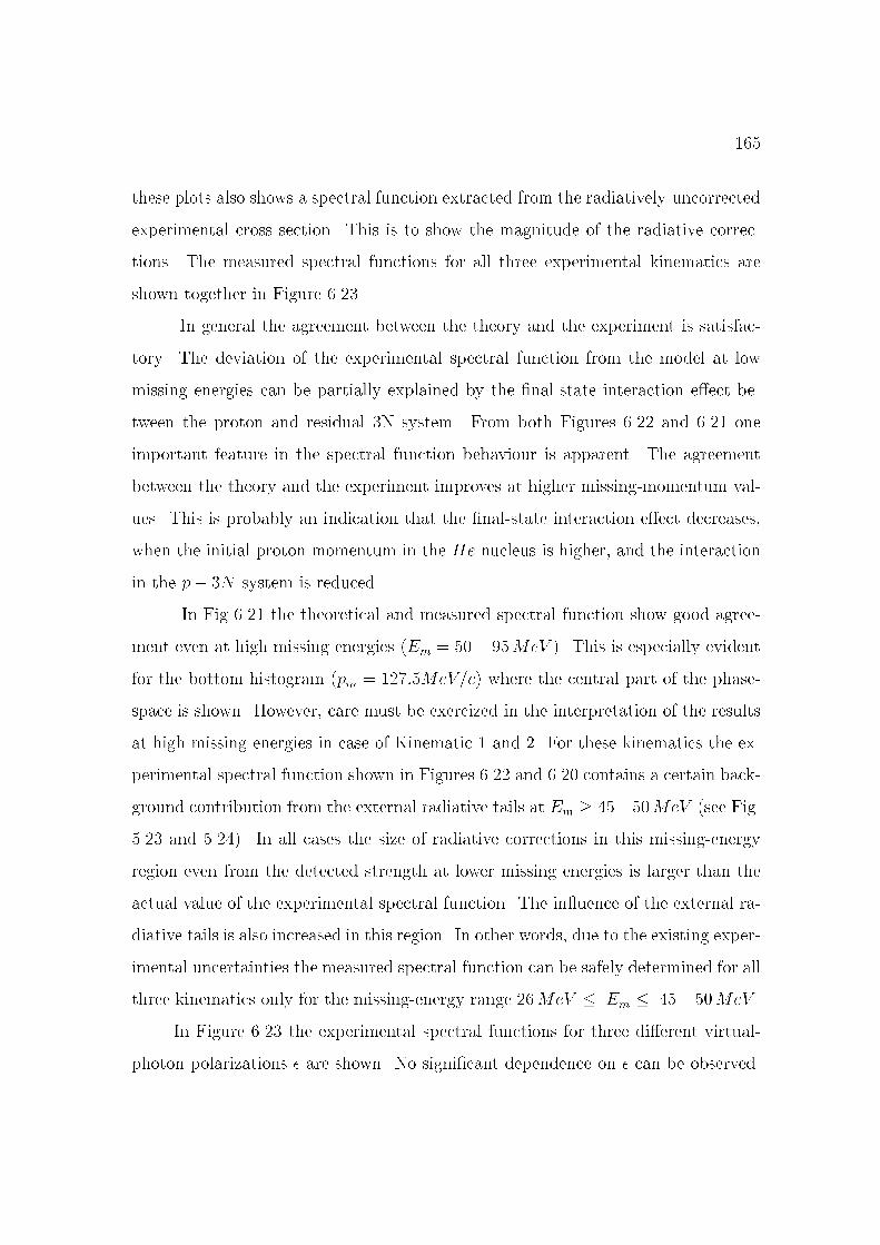
165

these plots also shows a spectral function extracted from the radiatively-uncorrected

experimental cross section. This is to show the magnitude of the radiative correc-

tions. The measured spectral functions for all three experimental kinematics are

shown together in Figure 6.23.

In general the agreement between the theory and the experiment is satisfac-

tory. The deviation of the experimental spectral function from the model at low

missing energies can be partially explained by the nal-state interaction eect be-

tween the proton and residual 3N system. From both Figures 6.22 and 6.21 one

important feature in the spectral function behaviour is apparent. The agreement

between the theory and the experiment improves at higher missing-momentum val-

ues. This is probably an indication that the nal-state interaction eect decreases,

when the initial proton momentum in the He nucleus is higher, and the interaction

in the p 3N system is reduced.

In Fig 6.21 the theoretical and measured spectral function show good agree-

ment even at high missing energies (E

m

= 50 95MeV ). This is especially evident

for the bottom histogram (p

m

= 127:5MeV=c) where the central part of the phase-

space is shown. However, care must be exercized in the interpretation of the results

at high missing energies in case of Kinematic 1 and 2. For these kinematics the ex-

perimental spectral function shown in Figures 6.22 and 6.20 contains a certain back-

ground contribution from the external radiative tails at E

m

4550MeV (see Fig.

5.23 and 5.24). In all cases the size of radiative corrections in this missing-energy

region even from the detected strength at lower missing energies is larger than the

actual value of the experimental spectral function. The in uence of the external ra-

diative tails is also increased in this region. In other words, due to the existing exper-

imental uncertainties the measured spectral function can be safely determined for all

three kinematics only for the missing-energy range 26MeV E

m

45 50MeV .

In Figure 6.23 the experimental spectral functions for three dierent virtual-

photon polarizations are shown. No signicant dependence on can be observed.

166

855.11 MeV (ε=0.60)

675.11 MeV (ε=0.37)

570.11 MeV (ε=0.16)

115< pm < 140 MeV/c

Em [MeV]

S(E

m,p

m) [

(GeV

)-3 (M

eV)-1

]

Efros et al.

0

0.2

0.4

0.6

0.8

1

1.2

1.4

15 20 25 30 35 40 45 50 55

Figure 6.23: Measured spectral function for all three kinematics

167

All measured spectral functions show a similar dependence from the missing energy

in a shape and magnitude.

6.3.3 The proton-momentum distribution

p

m

3;4

(p

m

) [(GeV=c)

3

]

MeV

c

855:11MeV 675:11MeV 855:11MeV

675:11MeV

570:11MeV

87.5 5:25 0:24 - - - -

92.5 5:05 0:22 - - - -

97.5 4:77 0:21 5:18 0:30 - - -

102.5 4:42 0:20 4:48 0:28 - - -

107.5 4:23 0:20 4:70 0:28 - - -

112.5 3:97 0:19 4:47 0:28 4:67 0:25 - -

117.5 3:48 0:19 3:99 0:28 4:20 0:23 4:21 0:28 4:80 0:41

122.5 3:68 0:19 3:53 0:27 4:39 0:22 3:70 0:27 4:01 0:39

127.5 3:19 0:18 3:08 0:26 3:79 0:21 3:23 0:26 4:12 0:39

132.5 3:28 0:18 3:40 0:26 4:18 0:21 3:51 0:26 4:08 0:38

137.5 3:08 0:18 2:87 0:25 3:90 0:21 3:04 0:25 3:21 0:36

142.5 2:95 0:17 2:93 0:24 3:69 0:22 3:19 0:26 3:15 0:35

147.5 2:51 0:17 2:94 0:24 3:37 0:23 3:19 0:27 3:28 0:35

152.5 2:62 0:17 2:90 0:23 3:55 0:25 3:36 0:29 4:08 0:38

157.5 2:42 0:17 3:08 0:24 - - -

162.5 2:25 0:18 - - - -

167.5 2:01 0:18 - - - -

172.5 1:88 0:19 - - - -

Table 6.3:

3;4

(p

m

) momentum distributions for

4

He(e; e

0

p)nd and

4

He(e; e

0

p)nn p reaction

channels (mark

is corresponding to the momentum distributions calculated with the !-

cut)

168

As was already shown in the previous section, the experimental spectral

functions for the three virtual-photon polarization values are similar within the

detected range of missing energy and missing momentum. In order to make more

a detailed comparison between these results, the experimental proton-momentum

distributions were calculated according to Equation 5.17 as:

3;4

(p

m

) =

45

Z

25

S(E

m

; p

m

) dE

m

(6.6)

The lower limit was selected to be less than the three-body breakup threshold in

order to include the continuum strength shifted to this region due to the nite

experimental energy resolution. All results were obtained for the case, both with

and without the !-cut.

Theoretical momentum distribution

The theoretical momentum distribution

3;4

(p

m

) was computed according to

Equation 6.6 using the theoretical spectral function obtained from ref. [54]. This

4

He spectral function was calculated with the Lorentz integral transform method

over a large missing-momentum range (see reference [55]). The semi-realistic Trento

N-N potential model was used. The nal-state interaction in the residual three-

nucleon system was completely taken into account.

Futher calculations that include the FSI eect between the detected proton

and the recoiling 3N system are required to compare the "distorted" experimental

proton-momentum distributions directly to the theoretical calculations.

Earlier experimental momentum distribution

Earlier the proton-momentum distributions for similar kinematical conditions

were measured by Florizone [23] at MAMI. These measurements were also performed

to study the L/T behaviour of the

4

He(e; e

0

p) cross section for three dierent

169


855.11 MeV (ε=0.60)

675.11 MeV (ε=0.37)

570.11 MeV (ε=0.16)

Florizone

Efros et al.

without ω-cut

pm [MeV/c]

ρ 3,4

[(Gev

/c)-3

]

2

4

6

8

10

12

14

0 20 40 60 80 100 120 140 160 180

Figure 6.24: The proton-momentum distribution

3;4

as a function of the missing momen-

tum

170

2

4

6

8

10

80 90 100 110 120 130 140 150 160 170 180


855.11 MeV (ε=0.60)675.11 MeV (ε=0.37)570.11 MeV (ε=0.16)FlorizoneEfros et al.

without ω-cut

pm [MeV/c]

ρ 3,4

[(Gev

/c)-3

]

with ω-cut

pm [MeV/c]

ρ 3,4

[(Gev

/c)-3

]

1

2

3

4

5

6

7

8

110 115 120 125 130 135 140 145 150 155

Figure 6.25: The proton-momentum distribution

3;4

as a function of the missing momen-

tum

171

0.002

0.004

0.006

0.008

0.01

0 20 40 60 80 100 120 140 160 180


855.11 MeV (ε=0.60)675.11 MeV (ε=0.37)570.11 MeV (ε=0.16)Florizone

Efros et al.

without ω-cut

pm [MeV/c]

N

∫4π ρ3,4(pm) (pm)2 dpm115

155

0.0280 ± 0.00160.0291 ± 0.00230.0349 ± 0.0035

-0.0368

855.11 MeV (ε=0.60)675.11 MeV (ε=0.37)570.11 MeV (ε=0.16)Florizone

Efros et al.

with ω-cut

pm [MeV/c]

N

∫4π ρ3,4(pm) (pm)2 dpm115

155

0.0354 ± 0.00210.0313 ± 0.00250.0349 ± 0.0035

-0.0368

0.002

0.004

0.006

0.008

0.01

100 110 120 130 140 150 160

Figure 6.26: hNi value as a function of the missing momentum (calculated for each missing-

momentum bin)

172

values (0.2, 0.45 and 0.64) and corresponding the beam energies of 540.11, 675.11

and 855.11 MeV. The momentum transfer ~q was the same as for our measurements

(685 MeV/c), but the !-value was 242.7 MeV, which corresponds to the top of the

quasi-elastic peak, where the scaling factor y = 0. All momentum distributions in

[23] were also extracted using the

cc1

prescription for the o-shell electron-proton

cross section. The systematic uncertainty for these results is 5-6 %. The error

bars shown in Figure 6.24 are statistical only. The major part of the data points

correspond to the lower missing momenta, but the overlap region between our results

is large and allows comparison with our measurements.

Analysis

Similar to the case of the two-body-breakup data analysis, the following di-

mensionless integral was calculated for comparison of the measured proton-momentum

distributions with the theory and each other

hNi = 4

155

Z

115

dp

m

p

2

m

3;4

(p

m

) (6.7)

for the missing-momentum range p

m

between the 115 and 155 MeV/c, which cor-

responds to the overlap region of the three kinematics for the continuum channels.

This averaged value hNi for the our kinematics and the theory is given in Figure 6.26.

The -dependence of the

3;4

(p

m

) was studied in the same way as for the

two-body breakup channel. First, the ratio

3;4

AV G

3;4

=

3;4

(p

m

; )

1

3

P

3;4

(p

m

; )

(6.8)

for each missing-momentum bin was calculated. This ratio shows how much the mo-

mentum distribution for each individual measurement deviates from the averaged

AV G

3;4

value for the particular p

m

bin. Second, the ratio

173

0.4

0.6

0.8

1

1.2

1.4

1.6

1.8

90 100 110 120 130 140 150 160 170 180


without ω-cut

pm [MeV/c]

Nex

pi /Nth

i

855.11 MeV (ε=0.60)675.11 MeV (ε=0.37)570.11 MeV (ε=0.16)

pm [MeV/c]

ΣNex

pi /ΣN

thi

0.4

0.5

0.6

0.7

0.8

0.9

1

1.1

1.2

1.3

115 120 125 130 135 140 145 150 155

Figure 6.27: Ratio for the experimental and theoretical momentum distributions as a

function of the missing momentum

174

0.2

0.4

0.6

0.8

1

1.2

1.4

1.6

1.8

115 120 125 130 135 140 145 150 155


855.11 MeV (ε=0.60)675.11 MeV (ε=0.37)570.11 MeV (ε=0.16)

pm [MeV/c]

ρ 3,4/

ρ 3,4A

VG

without ω-cut

855.11 MeV (ε=0.60)675.11 MeV (ε=0.37)570.11 MeV (ε=0.16)

pm [MeV/c]

ρ 3,4/

ρ 3,4A

VG

with ω-cut

0.2

0.4

0.6

0.8

1

1.2

1.4

1.6

1.8

115 120 125 130 135 140 145 150 155

Figure 6.28: The proton-momentum distributions compared to the averaged over the three

kinematics value

175

hNi

i

exp

hNi

i

th

=

exp

3;4

(p

i

m

)

th

3;4

(p

i

m

)

(6.9)

for each missing-momentum bin i (see Figures 6.27 and 6.29) was calculated. In

order to calculated the

th

3;4

value for each missing-momentum bin, the theoretical

data points were tted with a high-order polynomial, so that the functional depen-

dence

th

3;4

(p

m

) was extracted. The systematic uncertainty created by this procedure

was less than 2-3 %. After that the

th

3;4

was calculated for the missing-momentum

value corresponding to the middle of each missing-momentum bin. This ratio gives

the deviation of the experimental

exp

3;4

(p

m

) momentum distribution from the theory

prediction as a function of the missing momentum. Third, the the development of

the sum's ratio

P

i

hNi

i

exp

P

i

hNi

i

th

=

P

i

R

dp

m

h

(p

i

m

)

2

exp

3;4

(p

i

m

)

i

P

i

R

dp

m

h

(p

i

m

)

2

th

3;4

(p

i

m

)

i

(6.10)

was studied as a function of the missing momentum as shown in Figures 6.27 and

6.29.

Results

The large kinematic dependence seen for the data measured at dierent

in the 6-fold cross section was removed by dividing the cross sections by the fac-

tor p

2

p

cc1

ep

. The remaining dependence from the virtual-photon polarization was

studied both with and without the !-cut. When this cut is not used, the measured

momentum distributions show a signicant systematic dependence on . In Figure

6.28 (top picture), the data points measured at 570:11MeV incident-electron en-

ergy are systematically 15-20 % higher than the data collected at 855:11MeV and

675:11MeV , although the statistical uncertainty is large and the

3;4

=

AV G

3;4

value

176

0.4

0.6

0.8

1

1.2

1.4

1.6

1.8

110 115 120 125 130 135 140 145 150 155


pm [MeV/c]

with ω-cut

Nex

pi /Nth

i

855.11 MeV (ε=0.60)675.11 MeV (ε=0.37)570.11 MeV (ε=0.16)

pm [MeV/c]

with ω-cut

ΣNex

pi /ΣN

thi

0.4

0.5

0.6

0.7

0.8

0.9

1

1.1

1.2

1.3

1.4

115 120 125 130 135 140 145 150 155

Figure 6.29: Ratio for the experimental and theoretical momentum distributions as a

function of the missing momentum

177

uctuates from point to point. This dependence can be better observed in Figure

6.27, where the

P

hNi

i

exp

=

P

hNi

i

th

(bottom picture) and hNi

i

exp

=hNi

i

th

values are

shown. The integral value hNi calculated for the three kinematics and the theoret-

ical value are given in Figure 6.26. When the !-cut is not used, hNi value is higher

by approximately 20 % for the Kinematic 1 ( = 0.16) compare to the integral value

measured for the Kinematic 3 ( = 0.6).

This strong -dependence completely disappears in the data obtained with

the !-cut. In Figure 6.28 (bottom picture), no systematic -dependence can be ob-

served. The integral hNi value is also independent of the virtual-photon polarization

(see Figure 6.26).

In Figures 6.24, 6.24 and 6.26 measured-proton-momentum distributions are

also compared to the experimental results obtained earlier in Mainz and mentioned

in reference [23]. The agreement between those results and our measurements is

good, but the large statistical uncertainty for the data points from [23] are not al-

lowed more detailed study. In general, results measured at MAMI by Florizone are

lower by the 10-20 % compare to our measurements.

Without the !-cut the experimental momentum distributions are approxi-

mately 10-20 % lower than the theory predictions as shown in Figure 6.27. This

cuts removes almost all data dependence on and increases the hNi

i

exp

=hNi

i

th

up to

0.9 - 0.95.

This number is approximately 10 % higher than that for the two-body breakup

channel, where the experimental data points were approximately 20 % lower than

the theoretical predictions.

6.4 Systematic error estimate

The calculation of the systematic error due to the normalization procedure

was described in Chapter 4. It consists of a number of systematic uncertainties, and

178

is given in Table 4.6. The helium-target density value for elastic scattering, which

includes this systematic error, was used to calculate the helium-target density for

the individual (e,e'p) runs. The systematic uncertainty for the latest value includes,

in addition, a statistical error for the number of events detected in Spectrometer

C, and can be calculated from Equation 5.5. The next step is to calculate the

systematic normalization error for each kinematic according to Equation 5.6.

The total systematic error (=) in the (e,e'p) cross-section value due to

the helium-density calculation procedure was approximately 2.0 %, 2.2 % and 2.2 %

for Kinematic 1, 2 and 3 respectively.

The other systematic uncertainties were insignicant. The uncertainty in total

charge collected at the target and the coincidence dead-time error were of the order

of 0.1 % each, and were neglected. The sensitivity of the nal cross section to the

uncertainty in the beam energy and target-position error must be also small, because

even for the elastic measurements characterized by a strong angular dependence

these errors were of the order of 0.2 - 0.5 %. The contribution of the uncertainty

due to the software angular cuts was taken the same as for the elastic measurements

on He ( 0:4 0:6%).

Thus, the full systematic uncertainty (=) for the (e,e'p) cross section

measured in this experiment is 2.2-2.4 %.

Chapter 7

Conclusion

A high-resolution study of the

4

He(e; e

0

p) reaction was performed. The high

resolution of the Mainz spectrometers made it possible to study the two-body

breakup and continuum reaction channels separately. These measurements are also

characterized by a very low background, and therefore high data quality. The sys-

tematic error estimate for these measurements is 2:22:4 %. The following results

were obtained:

Two independent analysis methods (AEEXB simulations and RADCOR un-

folding) give a similar result concerning the problem of "unexpectedly large"

cross section for proton knockout observed in earlier (e,e'p) experiments in

the high missing-energy region (see Chapter 1). No such phenomenon was

observed in our measurements as shown in Figures 6.2, 6.21 and 7.1a. A large

strength observed in the raw (E

m

; p

m

) spectra in the high missing-energy re-

gion was formed by the radiative tails from the lower missing-energy regions.

The signicant non-zero strength seen in the high missing-energy region (and

also close to the phase-space boundaries) after the RADCOR unfolding be-

longs mostly to the external radiative tails from the outside of the detected

(E

m

; p

m

) region.

179

180

The 6-fold dierential cross section for the continuum channels of the

4

He(e; e

0

p)

reaction were measured in the missing-energy range 25 E

m

4550MeV .

The (e,e'p) cross section for E

m

50MeV shows no signicant deviation from

the model based on the theoretical spectral function from ref. [55]. At these

missing energies the measured strength is small and dominated by the radiative

background.

The Rosenbluth separation was performed for the two-body breakup cross

section averaged over the missing-momentum range 125 p

m

165MeV=c.

The experimental ratio for the longitudinal and transverse response functions

was calculated and compared to the prediction from the

cc1

o-shell e p

model of de Forest. The

L

=

T

value was 0:71 0:025, which is 33 % lower

than that from the

cc1

model. After including the systematic error the

L

=

T

value was 0:730:1 (31%13% below the prediction based on the

cc1

model

as shown in Figure 7.1c). This value is in a good agreement with the earlier

results presented by Ducret et al. [8], where the reduction of the L/T ratio

compare to the theory prediction was observed for the similar momentum

transfer ~q values.

The proton-triton momentum distributions also show systematic -dependence,

with a 6.6 % dierence for the integral hNi value between the kinematics with

the smallest and largest .

The measured proton-triton momentum distributions were found to be 15 -

25 % below the predictions from dierent theoretical models.

The Rosenbluth separation was also performed for the continuum cross section

averaged over the missing-momentum range 115 p

m

155MeV=c for a

number of the missing-energy values. The experimental ratio for the longitu-

dinal and transverse responses was calculated and compared to the prediction

from the

cc1

o-shell e p model of de Forest. The

L

=

T

value was found

181

to be in good agreement with the

cc1

model at low missing energies. In the

high missing-energy region of the measured (e,e'p) cross section, the L/T ra-

tio is signicantly reduced compared to the model as shown in Figure 7.1c.

The ratio (

L

=

T

)

exp

/(

L

=

T

)

cc1

was found to be (for the analysis with the

dierent missing-energy bin size): 0:67 0:21 (E

m

= 40MeV ), 0:59 0:34

(E

m

= 42:5MeV ), and 0:43 0:35 (E

m

= 43MeV ).

The distorted spectral function was measured in the missing-energy range

25 E

m

45 50MeV for all three kinematics. It was found that the

spectral function shows no signicant deviation from the theoretical spectral

function (ref. [55]) at E

m

50MeV (Fig. 6.21).

No signicant -dependence was observed for the spectral functions calculated

for the dierent kinematics (see Figure 7.1b).

No -dependence was observed for the proton-momentum distributions for the

continuum channel, when comparison is done for the same range of the energy-

transfer values. This result does not disagree with the Rosenbluth separation,

where the deviation from the

cc1

model was observed. In fact, the weight of

the events from the high missing-energy region is not large in the total inte-

gral value. The Rosenbluth separation thus permitted the L/T cross section

dependence to be studied in a more detailed way.

The proton-momentum distributions for the continuum channel were 4 - 15 %

below the theory prediction, when comparison is done for the same range of

the energy-transfer values.

In short, we can conclude: the majority of -dependence seen in the (e,e'p)

cross section for dierent kinematics is removed by division by the elementary e p

cross section in cc1 prescription of de Forest. A small remaining -dependence, which

probably indicates excess transverse strength is dicult to interprete uniquely due

182

0

0.5

1

1.5

15 20 25 30 35 40 45 50 55

0

0.5

1

1.5

15 20 25 30 35 40 45 50 55


855.11 MeV (ε=0.60)675.11 MeV (ε=0.37)570.11 MeV (ε=0.16)

115 < pm < 155 MeV/c

x10-9


d6 σ [fm

2 /(MeV

/c)2

/sr2 ] (a)

855.11 MeV (ε=0.60)675.11 MeV (ε=0.37)570.11 MeV (ε=0.16)

115 < pm < 140 MeV/c

Missing energy, [MeV]S(E m

,pm

) [(G

eV)-3

(MeV

)-1]

Efros et al.

(b)


(σL/σ

T)ex

p /(σL/σ

T)cc

1 (c)

0.5

1

15 20 25 30 35 40 45 50 55

Figure 7.1: Results shown as a function of missing energy. (a) Six-fold dierential cross

section for the three values of the virtual-photon polarization in the missing-momentum

range from 115 to 155 MeV/c. (b) Spectral function. (c) The ratio

L

=

T

(both the 2-body

and continuum channels)

to the relatively large systematic uncertainties. Futher attempts must be done

to reduce the systematic uncertainty due to the absolute data normalisation and

radiative unfolding procedure. More complete theoretical calculations that include

additional eects beyond PWIA (FSI, meson exchange currents and others) are also

183

required to make more detailed comparison between the experimental and theoretical

results.

Appendix A

A.1 GEANT model of the collimators

This part of the Appendix describes the GEANT models used to simulate

the collimators of the spectrometers in the new GEANT Monte-Carlo. The general

structure of the program is given in the Appendix C. Detailed description of the

collimators shape, and the computer codes used to generate the geometrical equiva-

lents of the collimators are included. The formulas used to calculate the geometrical

and angular constrains of the collimator of the Spectrometer B are also presented.

The shape of the collimators is quite complicated with the multiple faces in the

horizontal and vertical directions. In the new GEANT Monte-Carlo code described

in detail in Appendix C the collimators of Spectrometer A and B were both simu-

lated using the GEANT geometry package (reference [44]), with input parameters

for the real geometrical dimensions obtained from the original technical drawings.

A.1.1 The collimator of Spectrometer A

This collimator with an acceptance angle of 21 msr was successfully described

with 7 trapezoids of a TRD2 type (see reference [44]) which have x and y dimen-

sions both varying along the z axis as shown in Figure A.1. Both collimators were

manufactured from a heavy alloy containing 95 % of Tungsten with a density of ap-

proximately 18g=cm

3

, which was reproduced in the simulations. All trapezoids were

184

185

Main volume

Figure A.1: The collimator of Spectrometer A, the view from the spectrometer side

lled with the vacuum and positioned inside the main volume lled with Tungsten.

(Figure A.1).

A.1.2 The collimator of Spectrometer B

This collimator consists of four independent parts which can be moved in

order to set desired vertical angular acceptance values between 0 and 70 mrad and

horizontal angular acceptance between 0 and 20 mrad. The geometry of the col-

limator is described in details in Figure A.3, where the and are the nominal

values of the vertical and horizontal acceptance respectively. By using the relations

between the angular acceptance of the collimator and its geometrical dimensions

(shown in Figure A.3), an exact model of the collimator was implemented in the

GEANT simulation program. Figures A.4 and A.5 show how both the horizontal

and vertical components of the collimator were simulated by a number of trapezoids

of TRD2 type.

186

Main volume

PAR(1) = 40/2. ! x/2

PAR(2) = 30/2. ! y/2

PAR(3) = 8./2. ! z/2

call GSVOLU('AKOL','BOX ',2,PAR,3,IVOL)

rtf(1) = 60.55

rtf(2) = t0es

rtf(3) = f0es

call XYZRTP(xyzlab,rtf(1))

call GSPOS('AKOL',1,'BOX0',x,y,z,1,'ONLY')

1

st

volume

PAR(1) = 8.7211/2. ! x/2 at -z

PAR(2) = 8.8273 /2. ! x/2 at +z

PAR(3) = 7.9554/2. ! y/2 at -z

PAR(4) = 8.1511/2. ! y/2 at +z

PAR(5) = 1.600/2. ! z/2

call GSVOLU('HOA1','TRD2',3,PAR,5,IVOL)

x = 0.

y = 0.

z = -3.2

call GSPOS('HOA1',1,'AKOL',x,y,z,0,'ONLY')

2

nd

volume

PAR(1) = 8.8273/2. ! x/2 at -z

PAR(2) = 8.9356/2. ! x/2 at +z

PAR(3) = 8.1511/2. ! y/2 at -z

PAR(4) = 8.2734/2. ! y/2 at +z

PAR(5) = 1./2. ! z/2


x = 0.

y = 0.

z = -1.9


3

rd

volume

PAR(1) = 8.9356/2.

PAR(2) = 9.0006/2.

PAR(3) = 8.2734/2.

PAR(4) = 8.3573/2.

PAR(5) = 0.6/2.


x = 0.

y = 0.

z = -1.1


4

th

volume

PAR(1) = 9.0006/2.

PAR(2) = 9.2412/2.

PAR(3) = 8.3573/2.

PAR(4) = 8.5811/2.

PAR(5) = 1.6/2.


x = 0.

y = 0.

z = 0.


5

th

volume

PAR(1) = 9.2412/2.

PAR(2) = 9.3568/2.

PAR(3) = 8.5811/2.

PAR(4) = 8.6650/2.

PAR(5) = 0.6/2.


x = 0.

y = 0.

z = 1.1


6

th

volume

PAR(1) = 9.3568/2.

PAR(2) = 9.5494/2.

PAR(3) = 8.6650/2.

PAR(4) = 8.8224/2.

PAR(5) = 1./2.


x = 0.

y = 0.

z = 1.9


7

th

volume

PAR(1) = 9.5494/2.

PAR(2) = 9.9253/2.

PAR(3) = 8.8224/2.

PAR(4) = 9.0743/2.

PAR(5) = 1.6/2.


x = 0.

y = 0.

z = 3.2


Figure A.2: GEANT simulation of the collimator of Spectrometer A

187

33mm 34mm 33mm

x1 x2 x3x4

y1 y2 y3y4

y1=3368*tan

y2=3401*tan

y3=y2+34*tan(0.2+

y4=y3+33*tan(0.4+

x1=3144*tan

0.5 degrees

0.2 degrees

HORIZONTAL collimator

VERTICAL collimator

3368mm

~3144mm

x3=x2+34*tan(0.5+

x4=x3+33*tan(1+

Target

Target

Θ

)

)

φ

Θ

Θ

Θ

)

)φ

φ

Θ

φ

x2=3177*tanφ

Figure A.3: The geometry of the collimator of Spectrometer B, where and are the

angular acceptance values for a point target

188

Main volume

xtop=336.8*tan(colli(3)/1000.)

xbott=336.8*tan(colli(4)/1000.)

PAR(1)= 60./2. ! x/2

PAR(2)= 90./2. ! y/2

PAR(3)= 10./2. ! z/2

call GSVOLU('BKOV','BOX ',3,PAR,3,IVOL)

rtf(1)= 336.8+5.0 !dist. to the middle of vert.colli

rtf(2)= t0ps

rtf(3)= f0ps


call GSPOS('BKOV',1,'BOX0',x,y,z,2,'ONLY')

1st Top part

PAR(1)=50./2.

PAR(2)=50./2.

PAR(3)=20./2.

PAR(4)=PAR(3)-3.3*tan(colli(3)/1000.)

PAR(5)=3.3/2.

call GSVOLU('HBT1','TRD2 ',2,PAR,5,IVOL)

x=0.

y=xtop+20./2.

z=-5.+3.3/2.

call GSPOS('HBT1',1,'BKOV',x,y,z,0,'ONLY')

2nd Top part

PAR(1)=50./2.

PAR(2)=50./2.

PAR(3)=PAR(4)

PAR(4)=PAR(3)-3.4*tan(colli(3)/1000.+0.2*PI/180.)

PAR(5)=3.4/2.


x=0.

y=y

z=0.


3rd Top part

PAR(1)=50./2.

PAR(2)=50./2.

PAR(3)=PAR(4)


PAR(5)=3.3/2.


x=0.

y=y

z=5.-3.3/2.


1st Bottom part

PAR(1)=50./2.

PAR(2)=50./2.

PAR(3)=20./2.

PAR(4)=PAR(3)-3.3*tan(colli(4)/1000.)

PAR(5)=3.3/2.

call GSVOLU('HBB1','TRD2 ',2,PAR,5,IVOL)

x=0.

y=-xbott-20./2.

z=-5.+3.3/2.

call GSPOS('HBB1',1,'BKOV',x,y,z,0,'ONLY')

2nd Bottom part

PAR(1)=50./2.

PAR(2)=50./2.

PAR(3)=PAR(4)


PAR(5)=3.4/2.


x=0.

y=y

z=0.


3rd Bottom part

PAR(1)=50./2.

PAR(2)=50./2.

PAR(3)=PAR(4)


PAR(5)=3.3/2.


x=0.

y=y

z=5-3.3/2.


Figure A.4: GEANT simulation of the vertical collimator of Spectrometer B

189

Main volume

xleft=314.4*tan(colli(1)/1000.)

xrigh=314.4*tan(colli(2)/1000.)

PAR(1)= 60/2. ! x/2

PAR(2)= 70/2. ! y/2

PAR(3)= 10/2. ! z/2

call GSVOLU('BKOH','BOX ',3,PAR,3,IVOL)

rtf(1)= 314.4+5.0 ! distance to the middle of horiz.colli

rtf(2)= t0ps

rtf(3)= f0ps


call GSPOS('BKOH',1,'BOX0',x,y,z,2,'ONLY')

1st left part

PAR(1)=20./2.

PAR(2)=PAR(1)-3.3*tan(colli(1)/1000.)

PAR(3)=57./2.

PAR(4)=PAR(3)

PAR(5)=3.3/2.

call GSVOLU('HBL1','TRD2 ',2,PAR,5,IVOL)

x=-xleft-10.

y=0.

z=-5.+3.3/2.

call GSPOS('HBL1',1,'BKOH',x,y,z,0,'ONLY')

2nd left part

PAR(1)=PAR(2)


PAR(3)=57./2.

PAR(4)=57./2.

PAR(5)=3.4/2


x=x

y=0.

z=0.


3rd left part

PAR(1)=PAR(2)

PAR(2)=PAR(1)-3.3*tan(colli(1)/1000.+1.*PI/180.)

PAR(3)=57./2.

PAR(4)=57./2.

PAR(5)=3.3/2.


x=x

y=0.

z=5.-3.3/2.


1st right part

PAR(1)=20./2.

PAR(2)=PAR(1)-3.3*tan(colli(2)/1000.)

PAR(3)=57./2.

PAR(4)=PAR(3)

PAR(5)=3.3/2.

call GSVOLU('HBR1','TRD2 ',2,PAR,5,IVOL)

x=xrigh+10.

y=0.

z=-5.+3.3/2.

call GSPOS('HBR1',1,'BKOH',x,y,z,0,'ONLY')

2nd right part

PAR(1)=PAR(2)


PAR(3)=57./2.

PAR(4)=PAR(3)

PAR(5)=3.4/2.


x=x

y=0.

z=0.


3rd right part

PAR(1)=PAR(2)

PAR(2)=PAR(1)-3.3*tan(colli(2)/1000.+1.*PI/180.)

PAR(3)=57./2.

PAR(4)=PAR(3)

PAR(5)=3.3/2.


x=x

y=0.

z=5-3.3/2.


Figure A.5: GEANT simulation of the horizontal collimator of Spectrometer B

Appendix B

B.1 Monte-Carlo for calculations of

3;4

He(e; e

0

) elas-

tic cross sections

B.1.1 Overview

The new Monte-Carlo is the C++ code with two dierent operation modes,

(see Figure B.1). In the rst mode it calculates the cross section for elastic scat-

tering from

3;4

He averaged over the acceptance of Spectrometer A or B, based on

the known values of the helium form-factors from Equations 4.9 and 4.11. In the

second mode it returns the eective solid angle of Spectrometer A or B dependent

on dierent factors such as the beam rastering, extended target geometry, target

cell oset and the non-trivial geometrical shape of the collimators.

The new Monte-Carlo code took advantage of the C++ variant of the CERN

HBOOK libraries available in Mainz. These HMBook C++ libraries provide conve-

nient graphical output of all required values in a format used by the Mainz COLA++

program. This feature makes control of the calculations much easier and more e-

cient.

190

191

slit # x

i

[cm] y

i

[cm] R

i

0

[cm]

1 4.3606 3.9777 56.55

2 4.4137 4.0756 58.15

3 4.4678 4.1367 59.15

4 4.5003 4.1787 59.75

5 4.6206 4.2906 61.35

6 4.6784 4.3325 61.95

7 4.7747 4.4112 62.95

8 4.9626 4.5371 64.55

Table B.1: The horizontal x

i

and vertical y

i

dimensions of the 21 msr collimator of

Spectrometer A and the corresponding distances R

i

0

from the target

B.1.2 Events generation

The spectrometer eective solid angle

eff

was determined as a fraction of a total

solid angle

tot

sampled in the simulation:

eff

=

N

det

tot

N

tot

(B.1)

where N

det

is the number of events accepted by the spectrometer,

tot

and N

tot

are

the full solid angle and the number of events entering this solid angle.

tot

was

limited by the range of preselected spherical angles and to save the CPU time:

tot

= 4

(cos(

min

) cos(

max

))

2

(

max

min

)

360

(B.2)

The cross section calculations are made in the center-of-mass system and the

Lorentz transformation is used to obtain the corresponding values in the laboratory

system. The

eff

calculations were done completely in the laboratory frame.

192

Calculate cross-sectionCalculate effective solid agle

Fill all booked histograms,producePostscript filePrint out text output

If generated electron doesn’t hitany slit inside the collimator whenpassing through it, it is acceptedas a real event

From initial x,y,z coordinatesand spherical angles calculatex,y coordinates in the systemof spectrometer.

random selection.

momentum and factors.

Lorentz transformation of all kinematic values.Random selection.

functionof momentum and angles

transfer,Helium formfactors.

Spectrometer System

LAB System

Electron detectionOutput

CMS System

,

(mode #1)(mode #2) YES No electron

detected

New loop

Coulomb distortion of momentum

Calculate Gaussian resolutioncos

β γ

θ φCalculate electron energy and

Figure B.1: Simplied structure of the DUMP Monte-Carlo code

193

B.1.3 Simulation of physical processes

In order to obtain values for the cross section and eective solid angle that

were as close as possible to reality, the following setup details and corrections were

included in the calculations:

- beam rastering amplitudes;

- spherical shape of the target cell;

- possibility of changing the position of the target cell along the beam line;

- possibility of applying cuts on both

tgt

and

tgt

angles, as is done in the analysis

of the experimental data;

- average beam-energy losses in the helium gas and Al walls.

There were between 70 and 600 KeV for helium of density 0.04 g=cm

3

depending

on the vertex position inside the target cell.

- Coulomb distortion of momentum transfer.

When electrons approach the nucleus, the Coulomb eld accelerates them so that a

larger momentum transfer occurs. In the experimental form factors, used to make

predictions of the elastic cross section, the eect of Coulomb distortion was taken

into account. During the analysis of our experimental data, this eect remains

and therefore distortion of "pure" form factors by the nuclear Coulomb eld was

accounted for by introducing an eective momentum transfer q

eff

(see ref. [32]).

This resulted in 2% reduction of the calculated cross section:

q

eff

= q (1 +

1:5Z hc

p

beam

R

eq

) (B.3)

where R

eq

= 1:12 A

1=3

is the equivalent radius of a hard sphere, q is the 3-

momentum transfer [MeV], hc = 197.327 [ Mev fm ], = 1/137, p

beam

is the

electron beam momentum [MeV] , A=4 and Z=2.

- the simulation of momentum and angle resolution by Gaussian distributions based

on the experimental resolution of the spectrometers.

For these purposes the gasdev function obtained from reference [33], which gen-

194

erates a random Gaussian distribution with Mean=0 and =1 was used.

B.1.4 Particles tracking through the collimators

In the code, the shape of the 21 msr collimator of Spectrometer A was sim-

ulated by a number of slits of dened size, obtained from the original technical

drawings. The geometry of the collimator of Spectrometer B was calculated each

time using two input parameters for its vertical and horizontal acceptance as it is

shown in Figure A.3.

The following algorithm was used to simulate the correct tracking of the elec-

trons through a collimator. When an electron is passing through the collimator, the

x and y coordinates in the spectrometer coordinate system are calculated for each

slit of the collimator from the spherical

e

and

e

angles and the initial (x

w

; y

w

; z)

position of the reaction vertex according to Equations B.6 and B.7. This calcula-

tion requires the introduction of two additional variables,

x

and R

corr

0

, dened in

Equations B.4 and B.5.

x

= atan(tan(

e

)) cos(

0

e

) (B.4)

where

0

is equal to 180 degrees for Spectrometer A and 0 degrees for Spectrometer

B.

x

is in a reality a projection of

e

on the horizontal x z plane. R

corr

0

is a

distance from the reaction vertex (x

w

; y

w

; z) to a particular slit of the collimator:

R

corr

0

= R

0

(z

beam

+ z

abs

) cos(

0

) x

w

sin(

0

) (B.5)

where R

0

is a distance from the center of coordinates, where (x

w

= 0; y

w

= 0; z = 0)

to a particular slit of the collimator in the horizontal x z plane,

0

is the central

scattering angle of the spectrometer, z

beam

is the vertex position inside the target

cell and z

abs

is an absolute displacement of the target cell along the z axis. By

using all these variable the horizontal x and vertical y coordinates in the system of

coordinates of the spectrometers are calculated as:

x = R

corr

0

tan(

x

0

) (z

beam

+ z

abs

) sin(

0

) + x

w

cos(

0

) (B.6)

195

y =

p

(R

corr

0

)

2

+ x

2

sin(

x

) tan(

0

e

) + y

w

(B.7)

The vertical

spec

and horizontal

spec

angles at the target in the spectrometers

coordinate system were calculated as:

spec

= atan(y=R

corr

0

) (B.8)

spec

=

0

x

(B.9)

These two variables are used to place the cuts identical to those used during the

analysis of the experimental data.

For each slit the absolute x and y coordinates in the spectrometers coordinate

system were compared to the known geometrical dimensions corresponding to a

particular slit of the collimator. The true event means the electron drift through a

collimator volume without touching its walls.

B.1.5 Eective solid angle of the spectrometers

The solid angle of the spectrometers depends from the target position along

the y

0

coordinate of the spectrometer. A shift of the target position causes a change

of the absolute value of the spectrometer solid angle and the range of accessible

horizontal and vertical angles. By using a realistic model of the collimators these

changes were taken into account in calculating the elastic scattering cross sections

from carbon and helium targets. The range of eective solid angles for Spectrometers

A and B is shown in Figure B.2 as a function of y

0

. All the data points shown at

the plot were calculated using the DUMP Monte-Carlo code.

The eective solid angle of the spectrometers for the extended targets shows

only a minor dependence on y

0

. This is more evident for Spectrometer B, which has

much longer distance from the target to the collimator compared to Spectrometer

A. For Spectrometer A, the eective solid angle dependence, even for the maximum

extended target length of y

0

= 2:5 cm, is reduced by only 0:7 % compared to its

nominal value. In case of point targets, especially when the measured cross section

196

shows a strong angular dependence, changes of angular acceptance must be carefully

taken into account.

197

18.5

19

19.5

20

20.5

21

21.5

22

22.5

23

-3 -2 -1 0 1 2 3

Spectrometer A

y0 [cm]

Solid

ang

le [m

sr]

point targetextended target

y0 [cm]

Sol

id a

ngle

[msr

]

point target

extended target

Spectrometer B

5.45

5.5

5.55

5.6

5.65

5.7

5.75

5.8

-3 -2 -1 0 1 2 3

Figure B.2: The solid angle of Spectrometer A(B) as a function of the spectrometer y

0

coordinate in case of 21(5.6) msr collimator

Appendix C

C.1 GEANT Monte-Carlo code

C.1.1 Modeling of the experimental setup

As was explained in the Appendix A, realistic models of the collimators were

developed to describe the complicated geometrical acceptance of Spectrometers A

and B. The target cell was simulated as an Al cylinder lled with

4

He gas of density

as used in the experiment. It was assumed that 0:012 cm of mylar, and an air

of thickness of 6 cm (Spectrometer A) and 12 cm (Spectrometer B) were between

the target and the spectrometers. The scattering chamber was simulated as an Al

cylinder with a dened window size. It can be moved up and down by changing

one parameter in the GEANT input le. This option was incorporated to study

the eects of re-scattering from the scattering chamber windows. Details of the

scattering chamber geometry are given in Figure C.1.

C.1.2 Operation modes

The new program can be used in the following modes:

1) The simulation of the two-body and continuum breakup reactions on

3

He and

4

He start from the centre of mass system (CMS).

In this mode the program generates only events allowed by the energy-momentum

198

199

External windows (Al)

Top view 504mm scattering chamber itself Al

target cellbeam line

50mm

504mm

18 mm

1.5 mm

2 mm

23 mm

1 mm18 mm

25 mm

458 mm

Fe6 mm

Figure C.1: Scattering chamber

200

Track it throuh the cell.

2.Start kinematic subroutine

3.Track reaction electron

4.Track reaction proton

Fill all booked histogramsmomenta of detected particles

from All physical processes swithed ON Calculate Emiss,Pmiss from

vertex values of particles momentaMake cuts selectionsFill all booked histograms

1. Generate beam electron.

beam e reached vertex point

e detected

p detected

p not detected

Calculate Emiss,Pmiss

e not detected

True (e,e’p) detected

Modelling mode Detection volume calculations

Figure C.2: General structure of the GEANT Monte-Carlo code

201

conservation and can be used to reaction and background simulations. All phys-

ical processes, including nuclear interactions, can be switched on by setting the

corresponding parameters in the code input le. Internal bremsstrahlung also can

be included by using the method of two external eective radiators, which placed

before and after the reaction vertex (see reference [39]).

2) This mode is almost the same as the rst mode, accept that the electron arm of

the reaction is simulated in the laboratory frame . Again, only events allowed by

the energy-momentum conservation are generated. Further decay of the excited

compound particle X from the

3;4

He(e; eX) reaction is simulated in the CMS. The

mode was developed to save CPU time and improve a productivity of the code.

3) The detection-volume calculations were done completely in the laboratory frame

for the reaction:

e+

3;4

He! e

0

+ p+X

by uniformly sampling the 6-dimensional volume dp

e

dp

p

d

e

d

p

. In this mode,

external and internal bremsstrahlung are switched o, and particle ionization

losses are calculated as an average. Various software cuts identical to those used

in the analysis of the experimental data can be applied. Calculations of the o-

shell

ep

cross section in the cc1 prescription of de Forest are also included.

Appendix D

D.1 Helium-target density for the (e,e'p) runs

In this section, the luminosity information for the individual runs of

4

He(e; e

0

p)

measurements done at MAMI during June of 1998 is presented. For each kinematic,

two tables were used to give the information about the coincidence AB runs, and a

single Spectrometer C data.

In Tables D.1, D.3 and D.5 the luminosity information for Spectrometer C is

given. The values for total charge collected at the target Q

C

, the data-acquisition

deadtime, and the scaling factors for the single events detected in Spectrometer C

are shown there. The helium-target density

He

and the statistical error for the

number of single events detected in Spectrometer C are also included. More infor-

mation about these values can be nd in Chapter 5.

In Tables D.2, D.4 and D.6 the total charge collected at the target for the co-

incidence AB events and the coincidence dead-time values are shown. In addition,

the thickness of the helium target after the cut (2 cm) on z-target coordinate is

included.

The information included in these tables is sucient to normalize the exper-

imental yield, and calculate the cross-section values.

202

203

Run number Q

C

deadtime Scaling N

corr

He

He

N

corr

He

[mC] [%] [g=cm

3

] [%]

980618151844 95.859 2.0 25 12911.7 0.037810 0.45

980618161729 89.781 1.8 23 12997.4 0.038061 0.44

980618171815 89.584 1.9 23 13070.4 0.038275 0.44

980618181907 89.522 1.9 23 13083.8 0.038314 0.44

980618192129 92.623 1.9 23 12978.0 0.038005 0.44

980618203226 89.660 1.9 23 13006.6 0.038088 0.44

980618213309 90.581 1.9 23 13036.3 0.038175 0.44

980618223435 93.086 1.9 23 12970.8 0.037983 0.44

980618233733 36.511 1.9 23 13066.2 0.038263 0.70

Table D.1: Helium-target density at E

beam

= 570:11MeV

Run number Q

AB

[mC] deadtime %

He

[mg=cm

2

]

980618151844 95.856 6.0 151.24

980618161729 89.778 5.0 152.24

980618171815 89.589 5.0 153.10

980618181907 89.519 5.0 153.26

980618192129 92.628 5.0 152.02

980618203226 89.673 5.0 152.35

980618213309 90.584 5.0 152.70

980618223435 93.084 5.0 151.93

980618233733 36.514 5.0 153.05

Total 767.225 5.125 152.38

Table D.2: Helium-target thickness at E

beam

= 570:11MeV

204

Run number Q

C

Deadtime Scaling N

corr

He

He

N

corr

He

[mC] [%] [g=cm

3

] [%]

980620133354 89.379 1.8 20 11275.7 0.038055 0.45

980620143509 89.637 1.8 20 11185.2 0.037749 0.45

980620153604 89.328 1.8 20 11251.7 0.037974 0.45

980620163743 92.394 1.8 20 11244.2 0.037949 0.44

980620174037 67.531 1.8 20 11295.5 0.038122 0.51

980620184440 87.499 1.8 20 11212.7 0.037842 0.45

980620195512 34.667 1.8 20 11341.5 0.038277 0.71

980620202218 39.746 1.8 20 11246.3 0.037955 0.67

980620205440 20.187 1.5 20 11333.6 0.038250 0.93

980620214002 54.948 1.6 20 11362 0.038346 0.57


beam

= 675:11MeV

Run number Q

AB

[mC] Deadtime %

He

[mg=cm

2

]

980620133354 89.385 7.5 152.2

980620143509 89.651 7.5 151.0

980620153604 89.332 7.5 151.9

980620163743 92.399 7.5 151.8

980620174037 67.533 7.5 152.5

980620184440 87.502 7.5 151.4

980620195512 34.671 7.6 153.1

980620202218 39.749 7.5 151.8

980620205440 20.194 6.9 153.0

980620214002 54.947 6.9 153.4

Total 665.363 7.4 152.0


beam

= 675:11MeV

205

Run number Q

C

Deadtime Scaling N

corr

He

He

N

corr

He

[mC] [%] [g=cm

3

] [%]

980617044906 64.076 1.8 12 6054.85 0.038691 0.56

980617053232 45.233 1.8 12 6118.67 0.039099 0.66

980617060332 43.384 1.7 12 6071.33 0.038796 0.68

980617074433 45.223 1.7 12 6094.29 0.038943 0.67

980617081518 45.349 1.7 12 6066.06 0.038762 0.67

980617084825 45.897 1.7 12 6087.98 0.038903 0.66

980617092758 45.177 1.7 12 6065.73 0.038760 0.67

980617101452 47.124 1.7 12 6058.84 0.038716 0.65

980617110437 45.878 1.8 12 6104.03 0.039005 0.66

980617114913 45.266 1.7 12 6118.08 0.039095 0.66

980617122003 44.738 1.7 12 6103.54 0.039002 0.67


beam

= 855:11MeV

Run number Q

AB

[mC] Deadtime %

He

[mg=cm

2

]

980617044906 64.090 14.1 154.764

980617053232 45.254 14.1 156.396

980617060332 43.397 14.2 155.184

980617074433 45.242 14.1 155.772

980617081518 45.359 14.1 155.048

980617084825 45.922 14.2 155.612

980617092758 45.189 14.0 155.040

980617101452 47.147 14.4 154.864

980617110437 45.894 14.1 156.020

980617114913 45.274 14.1 156.380

980617122003 44.755 14.0 156.008


beam

= 855:11MeV

Bibliography

[1] y-dependence of Response-Function Separations on

3;4

He for 0 E

miss

100MeV , Proposal A1/3-96, Institut fuer Kernphysik, Mainz University, un-

published (http://wwwa1.kph.uni-mainz.de/A1/proposals.html)

[2] J. J. van Leeuwe et al, High missing-momentum components in

4

studied with

the (e,e'p) reaction, Proceedings of the 15

th

European Conf. on Few-Body Prob-

lems in Physics, Peniscola, 1995

[3] R. W. Lourie et al, Phys. Rev. Lett. 56, 2364 (1986)

[4] L. B. Weinstein et al, Phys. Rev. Lett. 64, 1646 (1990)

[5] L. J. H. M. Kester et al, Phys. Rev. Lett. B366, 44 (1996)

[6] P. E. Ulmer et al, Phys. Rev. Lett. 59, 2259 (1987)

[7] G. van der Steenhoven et al, Nucl. Phys. A484, 445 (1988)

[8] J.E. Ducret et al, Nucl. Phys. A553 (1993) 697

[9] R. Schiavilla, Phys. Rev. Lett. 65 (1990) 835

[10] Frank J, Hertz G 1914 Verh. Deutschen Phys. Ges. 16 457

[11] Fregeau J, Hofstadter R 1955 Phys. Rev. 99 1503

[12] T.W. Donnelly Advances in Nuclear Physics, Vol.22, p.67

206

207

[13] S. Bo et al., Nuclear Physics A435 (1985) 697

[14] T. de Forest, Nucl. Phys., A392, 232 (1983)

[15] G.G. Simon et al., Nuclear Physics A333 (1980), 381

[16] D. Mittwich, Diploma thesis, University of Mainz, unpublished, 1992

[17] S. Schardt, PhD thesis, University of Mainz, unpublished, 1994

(available at http://wwwa1.kph.uni-mainz.de/A1/publications.html#doc)

[18] Boeglin W.U. Czechoslovak J. of Physics, Vol.45 (1995), No.4/5

[19] K.I.Blomqvist et al., Nucl. Instr. and Meth., A403 (1998), 263-301

[20] M.W. Kuss, Technische Universitaet Darmstadt, PhD thesis, unpublished, 1996


[21] H.Merkel, Internal report, Institut fuer Kernphysik, Mainz University, 1997

[22] K. W. Krygier, PhD thesis, University of Mainz, unpublished, 1996


[23] R. Florizone, MIT, PhD thesis, unpublished, 1998


[24] J. Kelly, MIT, PhD thesis, unpublished, 1981

[25] C. R. Otterman et al., NPA436 (1985) 688

[26] J. Friedrich, University of Mainz, private communication

[27] T. Pospischil, University of Mainz, private communication

[28] M. Weis, University of Mainz, private communication

[29] K. Merle, PhD thesis, University of Mainz, unpublished, 1976

208

[30] M. Korn, PhD thesis, University of Mainz, unpublished, 1995


[31] J. Templon, University of Georgia, private communication

[32] J. Heisenberg and H.P. Block, Ann. Rev. Nucl. Part. Sci. 33 (1983) 569

[33] W.H. Press et al., Numerical recipes in C, Cambridge University Press

[34] A. Rokavec, University of Ljubljana, PhD thesis, unpublished, 1994

[35] J. Schwinger, Phys. Rev. 76, 790 (1949)

[36] J. Schwinger, Phys. Rev. 75, 898 (1949)

[37] S. Penner, Nuclear Structure Physics, Proceedings of the 18

th

Scottish Univer-

sity Summer School in Physics 1977

[38] J. Friedrich, Nucl. Instr. Meth. 129 (1975) 505

[39] L.W. Mo, Y.S. Tsai, Reviews of Modern Physics, Vol.41, N.1, January 1969

[40] W.R. Leo Techniques for Nuclear and Particle Physics Experiments, p.40

(Springer-Verlag, Berlin, 1987)

[41] J.A. Templon, Radiative-Tail Simulations for Mainz Expt. A1/1-93 (1998), In-

ternal report, University of Georgia

[42] C. E. Vellidis, AEEXB: A Program for Monte Carlo Simulations of coincidence

electron-scattering experiments, OOPS Collaboration Internal Report, MIT-

Bates Accelerator Laboratory, 1998

[43] J. A. Templon, C. E. Vellidis, R. E. J. Florizone, A. J. Sarty Phys. Rev. C 61,

014607 (2000)

[44] GEANT, CERN Program Library, Detector Description and Simulation Tool

209

[45] R. Schiavilla et al., Nucl. Phys. A449 219 (1986)

[46] I. E. Lagaris and V. R. Pandharipande, Nucl. Phys. A359 (1981) 331

[47] R. B. Wiringa et al., Phys. Rev. C29 (1984) 1207

[48] J.L. Forest et al., Phys. Rev C54, 646 (1996)

[49] http://www.phy.anl.gov/theory/research/overlap/he4.tp

[50] R. B. Wiringa et al., Phys. Rev. C51 (1995) 38

[51] B. S. Pudliner et al., Phys. Rev. Lett. 74 (1995) 4396

[52] J.F.J. van den Brand et all., Nucl. Phys. A534 (1991) 637

[53] J.J. Kelly Advances in Nuclear Phys., vol.23, p.75

[54] W. Leidemann, Trento University, private communication

[55] V. D. Efros, W. Leidemann, G. Orlandini, Phys. Rev. C58 (1998) 582

abstract - inspire hepinspirehep.net/record/1358293/files/kozlov.pdf · ingo ald, ew jan h riedric...

Documents