abstract interpretation (an introduction)
TRANSCRIPT
Abstract Interpretation (an introduction)
COST Action IC0701 - 2nd Action Training School
David Pichardie
INRIA Rennes, France
Introduction
Static program analysis
The goals of static program analysisI to prove properties about the run-time behaviour of a programI in a fully automatic wayI without actually executing this program
ApplicationsI code optimisationI error detection (array out of bound access, null pointers)I proof support (invariant extraction)
Abstract Interpretation 2 / 82
Introduction
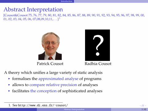
Abstract Interpretation[Cousot&Cousot 75, 76, 77, 79, 80, 81, 82, 84, 85, 86, 87, 88, 89, 90, 91, 92, 93, 94, 95, 96, 97, 98, 99, 00,01, 02, 03, 04, 05, 06, 07,08,09,10,11,. . . ] 1
?
2 / 2
Patrick Cousot Radhia Cousot
A theory which unifies a large variety of static analysisI formalises the approximated analyse of programsI allows to compare relative precision of analysesI facilitates the conception of sophisticated analyses
1. See http://www.di.ens.fr/˜cousot/Abstract Interpretation 3 / 82
Introduction
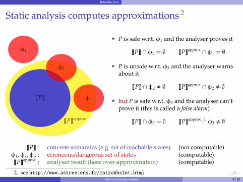
Static analysis computes approximations 2
φ1
φ2
φ3~P�
~P�approx
I P is safe w.r.t. φ1 and the analyser proves it
~P� ∩ φ1 = ∅ ~P�approx ∩ φ1 = ∅
I P is unsafe w.r.t. φ2 and the analyser warnsabout it
~P� ∩ φ2 , ∅ ~P�approx ∩ φ2 , ∅
I but P is safe w.r.t. φ3 and the analyser can’tprove it (this is called a false alarm)
~P� ∩ φ3 = ∅ ~P�approx ∩ φ3 , ∅
~P� : concrete semantics (e.g. set of reachable states) (not computable)φ1,φ2,φ3 : erroneous/dangerous set of states (computable)~P�approx : analyser result (here over-approximation) (computable)
2. see http://www.astree.ens.fr/IntroAbsInt.htmlAbstract Interpretation 4 / 82
Introduction
A flavor of abstract interpretation
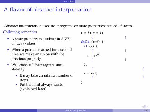
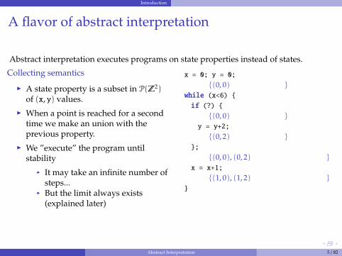
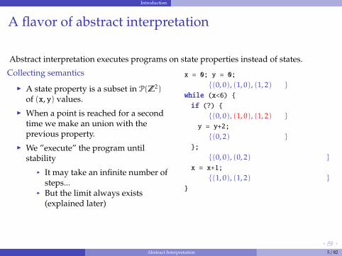
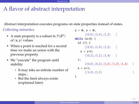
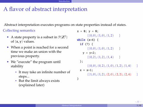
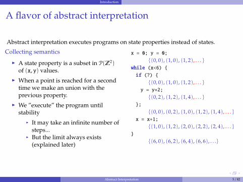
Abstract interpretation executes programs on state properties instead of states.
Collecting semantics
I A state property is a subset in P(Z2)of (x, y) values.
I When a point is reached for a secondtime we make an union with theprevious property.
I We ”execute” the program untilstability
I It may take an infinite number ofsteps...
I But the limit always exists(explained later)
x = 0; y = 0;
{
(0, 0), (1, 0), (1, 2), . . .
}
while (x<6) {
if (?) {
{
(0, 0), (1, 0), (1, 2), . . .
}
y = y+2;
{
(0, 2), (1, 2), (1, 4), . . .
}
};
{
(0, 0), (0, 2), (1, 0), (1, 2), (1, 4), . . .
}
x = x+1;
{
(1, 0), (1, 2), (2, 0), (2, 2), (2, 4), . . .
}
}
Abstract Interpretation 5 / 82
Introduction
A flavor of abstract interpretation
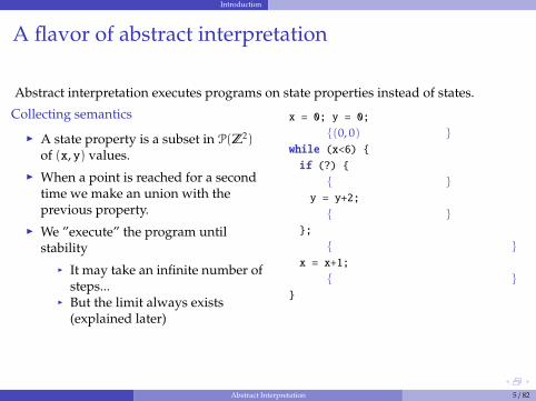
Abstract interpretation executes programs on state properties instead of states.
Collecting semantics
I A state property is a subset in P(Z2)of (x, y) values.
I When a point is reached for a secondtime we make an union with theprevious property.
I We ”execute” the program untilstability
I It may take an infinite number ofsteps...
I But the limit always exists(explained later)
x = 0; y = 0;
{(0, 0)
, (1, 0), (1, 2), . . .
}
while (x<6) {
if (?) {
{
(0, 0), (1, 0), (1, 2), . . .
}
y = y+2;
{
(0, 2), (1, 2), (1, 4), . . .
}
};
{
(0, 0), (0, 2), (1, 0), (1, 2), (1, 4), . . .
}
x = x+1;
{
(1, 0), (1, 2), (2, 0), (2, 2), (2, 4), . . .
}
}
Abstract Interpretation 5 / 82
Introduction
A flavor of abstract interpretation
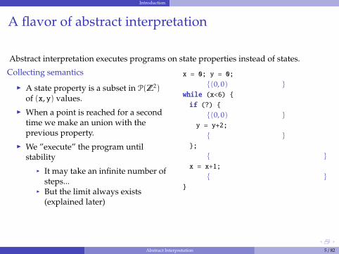
Abstract interpretation executes programs on state properties instead of states.
Collecting semantics
I A state property is a subset in P(Z2)of (x, y) values.
I When a point is reached for a secondtime we make an union with theprevious property.
I We ”execute” the program untilstability
I It may take an infinite number ofsteps...
I But the limit always exists(explained later)
x = 0; y = 0;
{(0, 0)
, (1, 0), (1, 2), . . .
}
while (x<6) {
if (?) {
{(0, 0)
, (1, 0), (1, 2), . . .
}
y = y+2;
{
(0, 2), (1, 2), (1, 4), . . .
}
};
{
(0, 0), (0, 2), (1, 0), (1, 2), (1, 4), . . .
}
x = x+1;
{
(1, 0), (1, 2), (2, 0), (2, 2), (2, 4), . . .
}
}
Abstract Interpretation 5 / 82
Introduction
A flavor of abstract interpretation
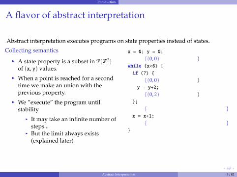
Abstract interpretation executes programs on state properties instead of states.
Collecting semantics
I A state property is a subset in P(Z2)of (x, y) values.
I When a point is reached for a secondtime we make an union with theprevious property.
I We ”execute” the program untilstability
I It may take an infinite number ofsteps...
I But the limit always exists(explained later)
x = 0; y = 0;
{(0, 0)
, (1, 0), (1, 2), . . .
}
while (x<6) {
if (?) {
{(0, 0)
, (1, 0), (1, 2), . . .
}
y = y+2;
{(0, 2)
, (1, 2), (1, 4), . . .
}
};
{
(0, 0), (0, 2), (1, 0), (1, 2), (1, 4), . . .
}
x = x+1;
{
(1, 0), (1, 2), (2, 0), (2, 2), (2, 4), . . .
}
}
Abstract Interpretation 5 / 82

Introduction
A flavor of abstract interpretation
Abstract interpretation executes programs on state properties instead of states.
Collecting semantics
I A state property is a subset in P(Z2)of (x, y) values.
I When a point is reached for a secondtime we make an union with theprevious property.
I We ”execute” the program untilstability
I It may take an infinite number ofsteps...
I But the limit always exists(explained later)
x = 0; y = 0;
{(0, 0)
, (1, 0), (1, 2), . . .
}
while (x<6) {
if (?) {
{(0, 0)
, (1, 0), (1, 2), . . .
}
y = y+2;
{(0, 2)
, (1, 2), (1, 4), . . .
}
};
{(0, 0), (0, 2)
, (1, 0), (1, 2), (1, 4), . . .
}
x = x+1;
{
(1, 0), (1, 2), (2, 0), (2, 2), (2, 4), . . .
}
}
Abstract Interpretation 5 / 82
Introduction
A flavor of abstract interpretation
Abstract interpretation executes programs on state properties instead of states.
Collecting semantics
I A state property is a subset in P(Z2)of (x, y) values.
I When a point is reached for a secondtime we make an union with theprevious property.
I We ”execute” the program untilstability
I It may take an infinite number ofsteps...
I But the limit always exists(explained later)
x = 0; y = 0;
{(0, 0)
, (1, 0), (1, 2), . . .
}
while (x<6) {
if (?) {
{(0, 0)
, (1, 0), (1, 2), . . .
}
y = y+2;
{(0, 2)
, (1, 2), (1, 4), . . .
}
};
{(0, 0), (0, 2)
, (1, 0), (1, 2), (1, 4), . . .
}
x = x+1;
{(1, 0), (1, 2)
, (2, 0), (2, 2), (2, 4), . . .
}
}
Abstract Interpretation 5 / 82

Introduction
A flavor of abstract interpretation
Abstract interpretation executes programs on state properties instead of states.
Collecting semantics
I A state property is a subset in P(Z2)of (x, y) values.
I When a point is reached for a secondtime we make an union with theprevious property.
I We ”execute” the program untilstability
I It may take an infinite number ofsteps...
I But the limit always exists(explained later)
x = 0; y = 0;
{(0, 0), (1, 0), (1, 2)
, . . .
}
while (x<6) {
if (?) {
{(0, 0)
, (1, 0), (1, 2), . . .
}
y = y+2;
{(0, 2)
, (1, 2), (1, 4), . . .
}
};
{(0, 0), (0, 2)
, (1, 0), (1, 2), (1, 4), . . .
}
x = x+1;
{(1, 0), (1, 2)
, (2, 0), (2, 2), (2, 4), . . .
}
}
Abstract Interpretation 5 / 82
Introduction
A flavor of abstract interpretation
Abstract interpretation executes programs on state properties instead of states.
Collecting semantics
I A state property is a subset in P(Z2)of (x, y) values.
I When a point is reached for a secondtime we make an union with theprevious property.
I We ”execute” the program untilstability
I It may take an infinite number ofsteps...
I But the limit always exists(explained later)
x = 0; y = 0;
{(0, 0), (1, 0), (1, 2)
, . . .
}
while (x<6) {
if (?) {
{(0, 0), (1, 0), (1, 2)
, . . .
}
y = y+2;
{(0, 2)
, (1, 2), (1, 4), . . .
}
};
{(0, 0), (0, 2)
, (1, 0), (1, 2), (1, 4), . . .
}
x = x+1;
{(1, 0), (1, 2)
, (2, 0), (2, 2), (2, 4), . . .
}
}
Abstract Interpretation 5 / 82

Introduction
A flavor of abstract interpretation
Abstract interpretation executes programs on state properties instead of states.
Collecting semantics
I A state property is a subset in P(Z2)of (x, y) values.
I When a point is reached for a secondtime we make an union with theprevious property.
I We ”execute” the program untilstability
I It may take an infinite number ofsteps...
I But the limit always exists(explained later)
x = 0; y = 0;
{(0, 0), (1, 0), (1, 2)
, . . .
}
while (x<6) {
if (?) {
{(0, 0), (1, 0), (1, 2)
, . . .
}
y = y+2;
{(0, 2), (1, 2), (1, 4)
, . . .
}
};
{(0, 0), (0, 2)
, (1, 0), (1, 2), (1, 4), . . .
}
x = x+1;
{(1, 0), (1, 2)
, (2, 0), (2, 2), (2, 4), . . .
}
}
Abstract Interpretation 5 / 82
Introduction
A flavor of abstract interpretation
Abstract interpretation executes programs on state properties instead of states.
Collecting semantics
I A state property is a subset in P(Z2)of (x, y) values.
I When a point is reached for a secondtime we make an union with theprevious property.
I We ”execute” the program untilstability
I It may take an infinite number ofsteps...
I But the limit always exists(explained later)
x = 0; y = 0;
{(0, 0), (1, 0), (1, 2)
, . . .
}
while (x<6) {
if (?) {
{(0, 0), (1, 0), (1, 2)
, . . .
}
y = y+2;
{(0, 2), (1, 2), (1, 4)
, . . .
}
};
{(0, 0), (0, 2), (1, 0), (1, 2), (1, 4)
, . . .
}
x = x+1;
{(1, 0), (1, 2), (2, 0), (2, 2), (2, 4)
, . . .
}
}
Abstract Interpretation 5 / 82
Introduction
A flavor of abstract interpretation
Abstract interpretation executes programs on state properties instead of states.
Collecting semantics
I A state property is a subset in P(Z2)of (x, y) values.
I When a point is reached for a secondtime we make an union with theprevious property.
I We ”execute” the program untilstability
I It may take an infinite number ofsteps...
I But the limit always exists(explained later)
x = 0; y = 0;
{(0, 0), (1, 0), (1, 2), . . . }while (x<6) {
if (?) {
{(0, 0), (1, 0), (1, 2), . . . }y = y+2;
{(0, 2), (1, 2), (1, 4), . . . }};
{(0, 0), (0, 2), (1, 0), (1, 2), (1, 4), . . . }x = x+1;
{(1, 0), (1, 2), (2, 0), (2, 2), (2, 4), . . . }}
{(6, 0), (6, 2), (6, 4), (6, 6), . . .}
Abstract Interpretation 5 / 82
Introduction
A flavor of abstract interpretation
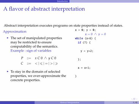
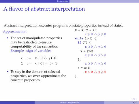
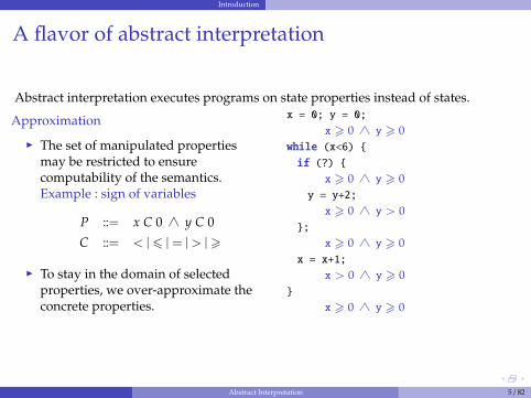
Abstract interpretation executes programs on state properties instead of states.
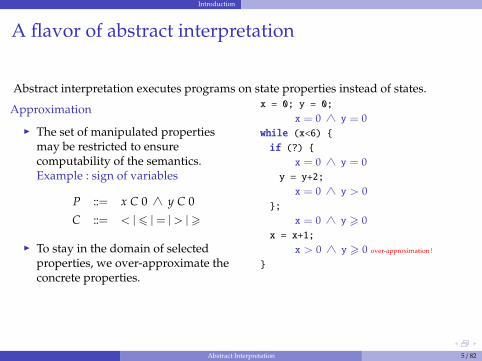
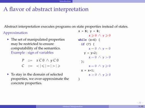
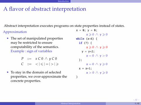
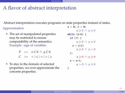
Approximation
I The set of manipulated propertiesmay be restricted to ensurecomputability of the semantics.Example : sign of variables
P ::= x C 0 ∧ y C 0
C ::= < | 6 | = | > | >
I To stay in the domain of selectedproperties, we over-approximate theconcrete properties.
x = 0; y = 0;
x = 0 ∧ y = 0while (x<6) {
if (?) {
y = y+2;
};
x = x+1;
}
Abstract Interpretation 5 / 82
Introduction
A flavor of abstract interpretation
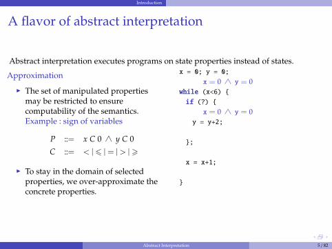
Abstract interpretation executes programs on state properties instead of states.
Approximation
I The set of manipulated propertiesmay be restricted to ensurecomputability of the semantics.Example : sign of variables
P ::= x C 0 ∧ y C 0
C ::= < | 6 | = | > | >
I To stay in the domain of selectedproperties, we over-approximate theconcrete properties.
x = 0; y = 0;
x = 0 ∧ y = 0while (x<6) {
if (?) {
x = 0 ∧ y = 0y = y+2;
};
x = x+1;
}
Abstract Interpretation 5 / 82
Introduction
A flavor of abstract interpretation
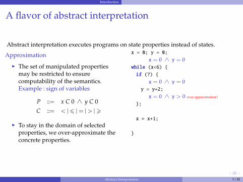
Abstract interpretation executes programs on state properties instead of states.
Approximation
I The set of manipulated propertiesmay be restricted to ensurecomputability of the semantics.Example : sign of variables
P ::= x C 0 ∧ y C 0
C ::= < | 6 | = | > | >
I To stay in the domain of selectedproperties, we over-approximate theconcrete properties.
x = 0; y = 0;
x = 0 ∧ y = 0while (x<6) {
if (?) {
x = 0 ∧ y = 0y = y+2;
x = 0 ∧ y > 0 over-approximation !
};
x = x+1;
}
Abstract Interpretation 5 / 82

Introduction
A flavor of abstract interpretation
Abstract interpretation executes programs on state properties instead of states.
Approximation
I The set of manipulated propertiesmay be restricted to ensurecomputability of the semantics.Example : sign of variables
P ::= x C 0 ∧ y C 0
C ::= < | 6 | = | > | >
I To stay in the domain of selectedproperties, we over-approximate theconcrete properties.
x = 0; y = 0;
x = 0 ∧ y = 0while (x<6) {
if (?) {
x = 0 ∧ y = 0y = y+2;
x = 0 ∧ y > 0};
x = 0 ∧ y > 0x = x+1;
}
Abstract Interpretation 5 / 82
Introduction
A flavor of abstract interpretation
Abstract interpretation executes programs on state properties instead of states.
Approximation
I The set of manipulated propertiesmay be restricted to ensurecomputability of the semantics.Example : sign of variables
P ::= x C 0 ∧ y C 0
C ::= < | 6 | = | > | >
I To stay in the domain of selectedproperties, we over-approximate theconcrete properties.
x = 0; y = 0;
x = 0 ∧ y = 0while (x<6) {
if (?) {
x = 0 ∧ y = 0y = y+2;
x = 0 ∧ y > 0};
x = 0 ∧ y > 0x = x+1;
x > 0 ∧ y > 0 over-approximation !
}
Abstract Interpretation 5 / 82
Introduction
A flavor of abstract interpretation
Abstract interpretation executes programs on state properties instead of states.
Approximation
I The set of manipulated propertiesmay be restricted to ensurecomputability of the semantics.Example : sign of variables
P ::= x C 0 ∧ y C 0
C ::= < | 6 | = | > | >
I To stay in the domain of selectedproperties, we over-approximate theconcrete properties.
x = 0; y = 0;
x > 0 ∧ y > 0while (x<6) {
if (?) {
x = 0 ∧ y = 0y = y+2;
x = 0 ∧ y > 0};
x = 0 ∧ y > 0x = x+1;
x > 0 ∧ y > 0}
Abstract Interpretation 5 / 82
Introduction
A flavor of abstract interpretation
Abstract interpretation executes programs on state properties instead of states.
Approximation
I The set of manipulated propertiesmay be restricted to ensurecomputability of the semantics.Example : sign of variables
P ::= x C 0 ∧ y C 0
C ::= < | 6 | = | > | >
I To stay in the domain of selectedproperties, we over-approximate theconcrete properties.
x = 0; y = 0;
x > 0 ∧ y > 0while (x<6) {
if (?) {
x > 0 ∧ y > 0y = y+2;
x = 0 ∧ y > 0};
x = 0 ∧ y > 0x = x+1;
x > 0 ∧ y > 0}
Abstract Interpretation 5 / 82

Introduction
A flavor of abstract interpretation
Abstract interpretation executes programs on state properties instead of states.
Approximation
I The set of manipulated propertiesmay be restricted to ensurecomputability of the semantics.Example : sign of variables
P ::= x C 0 ∧ y C 0
C ::= < | 6 | = | > | >
I To stay in the domain of selectedproperties, we over-approximate theconcrete properties.
x = 0; y = 0;
x > 0 ∧ y > 0while (x<6) {
if (?) {
x > 0 ∧ y > 0y = y+2;
x > 0 ∧ y > 0};
x = 0 ∧ y > 0x = x+1;
x > 0 ∧ y > 0}
Abstract Interpretation 5 / 82
Introduction
A flavor of abstract interpretation
Abstract interpretation executes programs on state properties instead of states.
Approximation
I The set of manipulated propertiesmay be restricted to ensurecomputability of the semantics.Example : sign of variables
P ::= x C 0 ∧ y C 0
C ::= < | 6 | = | > | >
I To stay in the domain of selectedproperties, we over-approximate theconcrete properties.
x = 0; y = 0;
x > 0 ∧ y > 0while (x<6) {
if (?) {
x > 0 ∧ y > 0y = y+2;
x > 0 ∧ y > 0};
x > 0 ∧ y > 0x = x+1;
x > 0 ∧ y > 0}
x > 0 ∧ y > 0
Abstract Interpretation 5 / 82
Introduction
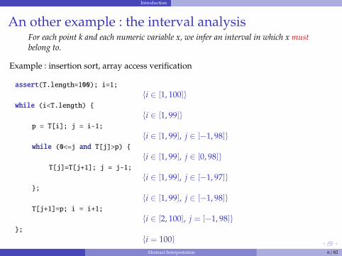
An other example : the interval analysisFor each point k and each numeric variable x, we infer an interval in which x mustbelong to.
Example : insertion sort, array access verification
assert(T.length=100); i=1;
{i ∈ [1, 100]}while (i<T.length) {
{i ∈ [1, 99]}p = T[i]; j = i-1;
{i ∈ [1, 99], j ∈ [−1, 98]}while (0<=j and T[j]>p) {
{i ∈ [1, 99], j ∈ [0, 98]}T[j]=T[j+1]; j = j-1;
{i ∈ [1, 99], j ∈ [−1, 97]}};
{i ∈ [1, 99], j ∈ [−1, 98]}T[j+1]=p; i = i+1;
{i ∈ [2, 100], j = [−1, 98]}};
{i = 100}Abstract Interpretation 6 / 82
Introduction
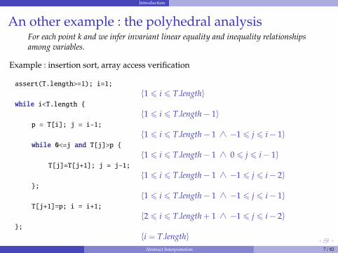
An other example : the polyhedral analysisFor each point k and we infer invariant linear equality and inequality relationshipsamong variables.
Example : insertion sort, array access verification
assert(T.length>=1); i=1;
{1 6 i 6 T.length}while i<T.length {
{1 6 i 6 T.length − 1}p = T[i]; j = i-1;
{1 6 i 6 T.length − 1 ∧ −1 6 j 6 i − 1}while 0<=j and T[j]>p {
{1 6 i 6 T.length − 1 ∧ 0 6 j 6 i − 1}T[j]=T[j+1]; j = j-1;
{1 6 i 6 T.length − 1 ∧ −1 6 j 6 i − 2}};
{1 6 i 6 T.length − 1 ∧ −1 6 j 6 i − 1}T[j+1]=p; i = i+1;
{2 6 i 6 T.length + 1 ∧ −1 6 j 6 i − 2}};
{i = T.length}Abstract Interpretation 7 / 82
Introduction
This lecture
1 Introduction
2 Intermediate representation : syntax and semantics
3 Collecting semantics
4 Just put some ]...
5 Building a generic abstract interpreter
6 Numeric abstraction by intervals
7 Widening/Narrowing
8 Polyhedral abstract interpretation
9 Readings
Abstract Interpretation 8 / 82
Intermediate representation : syntax and semantics
Outline
1 Introduction
2 Intermediate representation : syntax and semantics
3 Collecting semantics
4 Just put some ]...
5 Building a generic abstract interpreter
6 Numeric abstraction by intervals
7 Widening/Narrowing
8 Polyhedral abstract interpretation
9 Readings
Abstract Interpretation 9 / 82
Intermediate representation : syntax and semantics
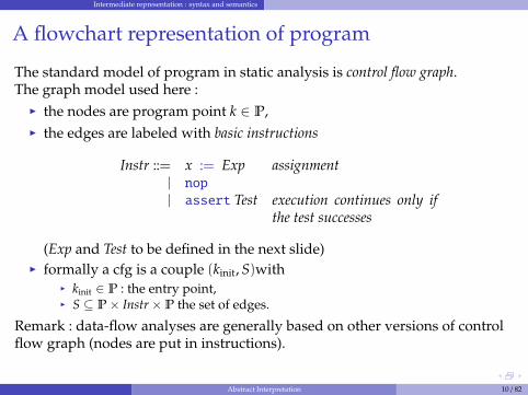
A flowchart representation of program
The standard model of program in static analysis is control flow graph.The graph model used here :I the nodes are program point k ∈ P,I the edges are labeled with basic instructions
Instr ::= x := Exp assignment| nop
| assert Test execution continues only ifthe test successes
(Exp and Test to be defined in the next slide)I formally a cfg is a couple (kinit, S)with
I kinit ∈ P : the entry point,I S ⊆ P× Instr× P the set of edges.
Remark : data-flow analyses are generally based on other versions of controlflow graph (nodes are put in instructions).
Abstract Interpretation 10 / 82
Intermediate representation : syntax and semantics
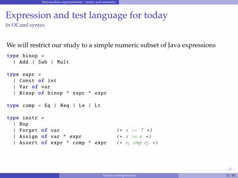
Expression and test language for todayIn OCaml syntax
We will restrict our study to a simple numeric subset of Java expressions
type binop =| Add | Sub | Mult
type expr =| Const of int| Var of var| Binop of binop * expr * expr
type comp = Eq | Neq | Le | Lt
type instr =| Nop
| Forget of var ( ∗ x := ? ∗ )| Assign of var * expr ( ∗ x := e ∗ )| Assert of expr * comp * expr ( ∗ e1 cmp e2 ∗ )
Abstract Interpretation 11 / 82
Intermediate representation : syntax and semantics
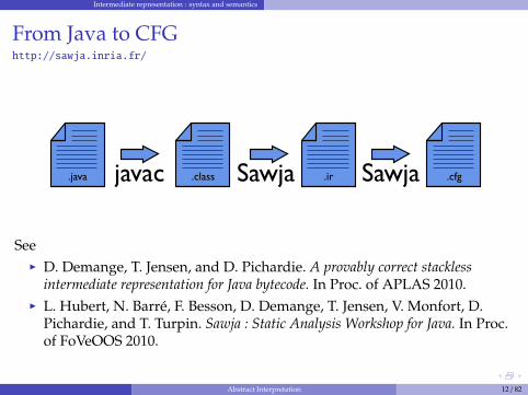
From Java to CFGhttp://sawja.inria.fr/
.java .class .ir .cfgjavac SawjaSawja
SeeI D. Demange, T. Jensen, and D. Pichardie. A provably correct stackless
intermediate representation for Java bytecode. In Proc. of APLAS 2010.I L. Hubert, N. Barre, F. Besson, D. Demange, T. Jensen, V. Monfort, D.
Pichardie, and T. Turpin. Sawja : Static Analysis Workshop for Java. In Proc.of FoVeOOS 2010.
Abstract Interpretation 12 / 82

Demo
Intermediate representation : syntax and semantics
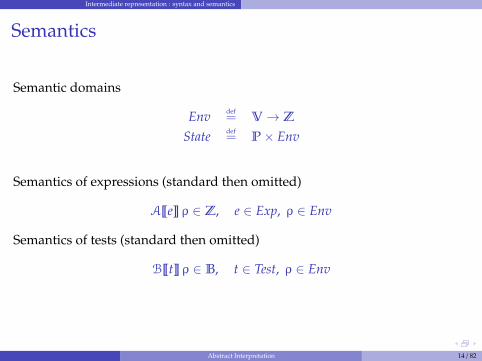
Semantics
Semantic domains
Env def= V→ Z
State def= P× Env
Semantics of expressions (standard then omitted)
A~e� ρ ∈ Z, e ∈ Exp, ρ ∈ Env
Semantics of tests (standard then omitted)
B~t� ρ ∈ B, t ∈ Test, ρ ∈ Env
Abstract Interpretation 14 / 82
Intermediate representation : syntax and semantics
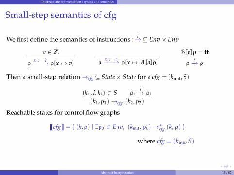
Small-step semantics of cfg
We first define the semantics of instructions : i−→⊆ Env× Env
v ∈ Zρ
x := ?−−−→ ρ[x 7→ v] ρx := a−−−→ ρ[x 7→ A[[a]]ρ]
B[[t]]ρ = tt
ρt−→ ρ
Then a small-step relation→cfg⊆ State× State for a cfg = (kinit, S)
(k1, i, k2) ∈ S ρ1i−→ ρ2
(k1, ρ1)→cfg (k2, ρ2)
Reachable states for control flow graphs�
cfg�
= { (k, ρ) | ∃ρ0 ∈ Env, (kinit, ρ0)→∗cfg (k, ρ) }
where cfg = (kinit, S)
Abstract Interpretation 15 / 82
Intermediate representation : syntax and semantics
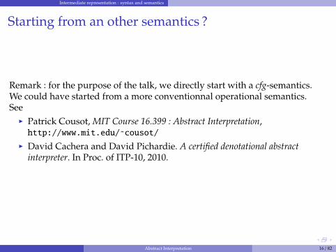
Starting from an other semantics ?
Remark : for the purpose of the talk, we directly start with a cfg-semantics.We could have started from a more conventionnal operational semantics.SeeI Patrick Cousot, MIT Course 16.399 : Abstract Interpretation,http://www.mit.edu/˜cousot/
I David Cachera and David Pichardie. A certified denotational abstractinterpreter. In Proc. of ITP-10, 2010.
Abstract Interpretation 16 / 82
Collecting semantics
Outline
1 Introduction
2 Intermediate representation : syntax and semantics
3 Collecting semantics
4 Just put some ]...
5 Building a generic abstract interpreter
6 Numeric abstraction by intervals
7 Widening/Narrowing
8 Polyhedral abstract interpretation
9 Readings
Abstract Interpretation 17 / 82
Collecting semantics
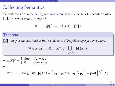
Collecting SemanticsWe will consider a collecting semantics that give us the set of reachable states�
p�col
k at each program points k.
∀k ∈ P,�
p�col
k = { ρ | (k, ρ) ∈ �p� }
Theorem�
p�col may be characterized as the least fixpoint of the following equation system.
∀k ∈ labels(p), Xk = Xinitk ∪
⋃
(k′,i,k)∈p
~i� (Xk′)
with Xinitk =
{Env if k = kinit∅ otherwise
and
∀i ∈ Instr, ∀X ⊆ Env, ~i� (X) ={ρ2 | ∃ρ1 ∈ X, ρ1
i−→ ρ2
}= post
[i−→](X)
Abstract Interpretation 18 / 82
Collecting semantics
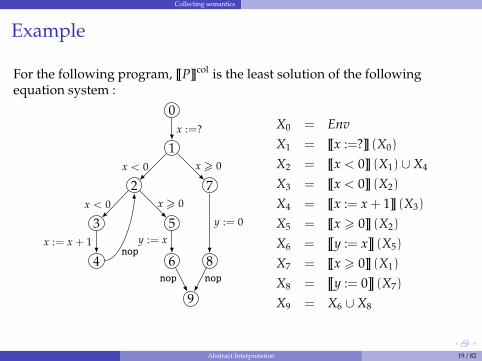
Example
For the following program, ~P�col is the least solution of the followingequation system :
0
1
2
3
4
5
6
7
8
9
x :=?
x < 0
x < 0
x > 0
x := x + 1nop
x > 0
y := x
y := 0
nop nop
X0 = EnvX1 = ~x :=?� (X0)
X2 = ~x < 0� (X1) ∪ X4
X3 = ~x < 0� (X2)
X4 = ~x := x + 1� (X3)
X5 = ~x > 0� (X2)
X6 =�
y := x�
(X5)
X7 = ~x > 0� (X1)
X8 =�
y := 0�
(X7)
X9 = X6 ∪ X8
Abstract Interpretation 19 / 82
Collecting semantics
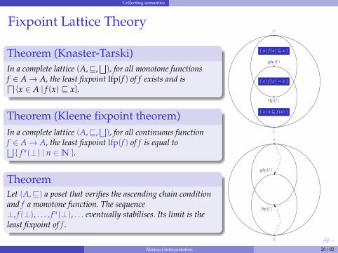
Fixpoint Lattice Theory
Theorem (Knaster-Tarski)In a complete lattice (A,v,
⊔), for all monotone functions
f ∈ A→ A, the least fixpoint lfp(f ) of f exists and is�
{x ∈ A | f (x) v x}.
Theorem (Kleene fixpoint theorem)In a complete lattice (A,v,
⊔), for all continuous function
f ∈ A→ A, the least fixpoint lfp(f ) of f is equal to⊔{ f n(⊥) | n ∈N }.
TheoremLet (A,v) a poset that verifies the ascending chain conditionand f a monotone function. The sequence⊥, f (⊥), . . . , f n(⊥), . . . eventually stabilises. Its limit is theleast fixpoint of f .
Lattice theory Fixpoints
Fixpoints, post-fixpoints and pre-fixpoints
gfp(f)
lfp(f)
�
⊥
{ x | f(x) = x }
{ x | f(x) � x }
{ x | x � f(x) }
� =�
{ x | f (x) � x }
gfp(f ) =�
{ x | x � f (x) }
lfp(f ) =�
{ x | f (x) � x }
⊥ =�
{ x | x � f (x) }
Static analysis 35 / 68
Lattice theory Fixpoints
Fixpoint computation
gfp(f)
lfp(f)
�
⊥⊥, f(⊥), . . . , f n(⊥), . . . , lfp f
�, f(�), . . . , f n(�), . . . , gfp f
Static analysis 40 / 68
Abstract Interpretation 20 / 82
Collecting semantics
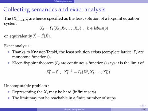
Collecting semantics and exact analysisThe (Xk)i=1..N are hence specified as the least solution of a fixpoint equationsystem
Xk = Fk(X1, X2, . . . , XN) , k ∈ labels(p)
or, equivalently ~X = ~F(~X).
Exact analysis :I Thanks to Knaster-Tarski, the least solution exists (complete lattice, Fk are
monotone functions),I Kleen fixpoint theorem (Fk are continuous functions) says it is the limit of
X0k = ∅ , Xn+1
k = Fk(Xn1 , Xn
2 , . . . , XnN)
Uncomputable problem :I Representing the Xk may be hard (infinite sets)I The limit may not be reachable in a finite number of steps
Abstract Interpretation 21 / 82
Collecting semantics
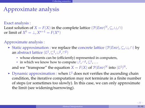
Approximate analysis
Exact analysis :Least solution of X = F(X) in the complete lattice (P(Env)N,⊆,∪,∩)or limit of X0 = ⊥, Xn+1 = F(Xn)
Approximate analysis :I Static approximation : we replace the concrete lattice (P(Env),⊆,∪,∩) by
an abstract lattice (L],v],t],u])I whose elements can be (efficiently) represented in computers,I in which we know how to compute t], u], v], . . .
and we “transpose” the equation X = F(X) of P(Env)N into (L])N.I Dynamic approximation : when L] does not verifies the ascending chain
condition, the iterative computation may not terminate in a finite numberof steps (or sometimes too slowly). In this case, we can only approximatethe limit (see widening/narrowing).
Abstract Interpretation 22 / 82
Just put some ] ...
Outline
1 Introduction
2 Intermediate representation : syntax and semantics
3 Collecting semantics
4 Just put some ]...
5 Building a generic abstract interpreter
6 Numeric abstraction by intervals
7 Widening/Narrowing
8 Polyhedral abstract interpretation
9 Readings
Abstract Interpretation 23 / 82
Just put some ] ...
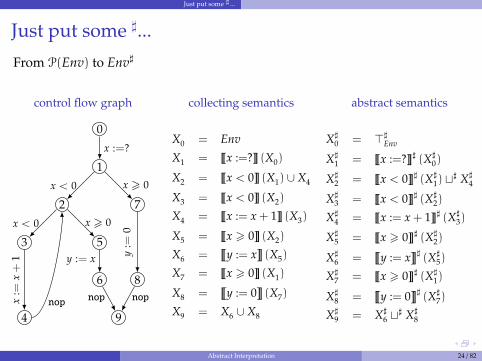
Just put some ]...
From P(Env) to Env]
control flow graph
0
1
2
3
4
5
6
7
8
9
x :=?
x < 0
x < 0
x > 0
x:=
x+
1
nop
x > 0
y := x y:=
0
nop nop
collecting semantics
X0 = EnvX1 = ~x :=?� (X0)
X2 = ~x < 0� (X1) ∪ X4
X3 = ~x < 0� (X2)
X4 = ~x := x + 1� (X3)
X5 = ~x > 0� (X2)
X6 =�
y := x�
(X5)
X7 = ~x > 0� (X1)
X8 =�
y := 0�
(X7)
X9 = X6 ∪ X8
abstract semantics
X]0 = >]
Env
X]1 = ~x :=?�] (X]
0)
X]2 = ~x < 0�] (X]
1) t] X]4
X]3 = ~x < 0�] (X]
2)
X]4 = ~x := x + 1�] (X]
3)
X]5 = ~x > 0�] (X]
2)
X]6 =
�
y := x�]
(X]5)
X]7 = ~x > 0�] (X]
1)
X]8 =
�
y := 0�]
(X]7)
X]9 = X]
6 t] X]8
Abstract Interpretation 24 / 82
Just put some ] ...
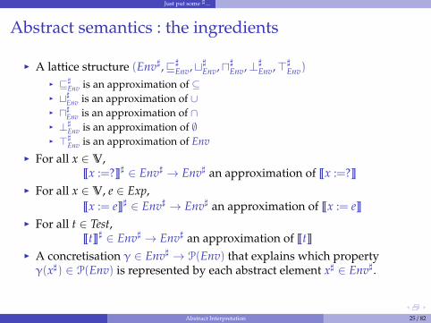
Abstract semantics : the ingredients
I A lattice structure (Env],v]Env,t]Env,u]Env,⊥]
Env,>]Env)
I v]Env is an approximation of ⊆
I t]Env is an approximation of ∪
I u]Env is an approximation of ∩
I ⊥]Env is an approximation of ∅
I >]Env is an approximation of Env
I For all x ∈ V,~x :=?�] ∈ Env] → Env] an approximation of ~x :=?�
I For all x ∈ V, e ∈ Exp,~x := e�] ∈ Env] → Env] an approximation of ~x := e�
I For all t ∈ Test,~t�] ∈ Env] → Env] an approximation of ~t�
I A concretisation γ ∈ Env] → P(Env) that explains which propertyγ(x]) ∈ P(Env) is represented by each abstract element x] ∈ Env].
Abstract Interpretation 25 / 82
Just put some ] ...
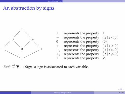
An abstraction by signs
−0 +0
− 0 +
⊥
>⊥ represents the property ∅− represents the property { z | z < 0 }
0 represents the property {0}+ represents the property { z | z > 0 }
−0 represents the property { z | z 6 0 }
+0 represents the property { z | z > 0 }
> represents the property Z
Env] def= V→ Sign : a sign is associated to each variable.
Abstract Interpretation 26 / 82
Just put some ] ...
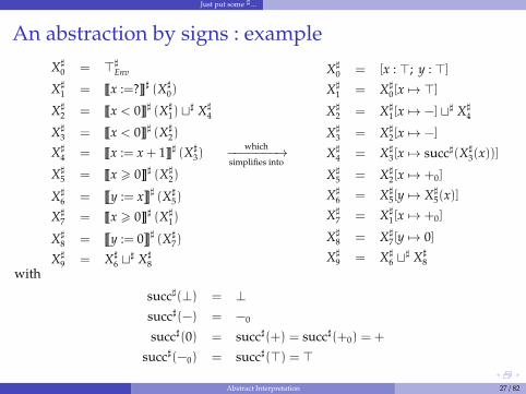
An abstraction by signs : exampleX]
0 = >]Env
X]1 = ~x :=?�] (X]
0)
X]2 = ~x < 0�] (X]
1) t] X]4
X]3 = ~x < 0�] (X]
2)
X]4 = ~x := x + 1�] (X]
3)
X]5 = ~x > 0�] (X]
2)
X]6 =
�
y := x�]
(X]5)
X]7 = ~x > 0�] (X]
1)
X]8 =
�
y := 0�]
(X]7)
X]9 = X]
6 t] X]8
which−−−−−−−→simplifies into
X]0 = [x : >; y : >]
X]1 = X]
0[x 7→ >]X]
2 = X]1[x 7→ −] t] X]
4
X]3 = X]
2[x 7→ −]
X]4 = X]
3[x 7→ succ](X]3(x))]
X]5 = X]
2[x 7→ +0]
X]6 = X]
5[y 7→ X]5(x)]
X]7 = X]
1[x 7→ +0]
X]8 = X]
7[y 7→ 0]
X]9 = X]
6 t] X]8
with
succ](⊥) = ⊥succ](−) = −0
succ](0) = succ](+) = succ](+0) = +
succ](−0) = succ](>) = >
Abstract Interpretation 27 / 82
Just put some ] ...
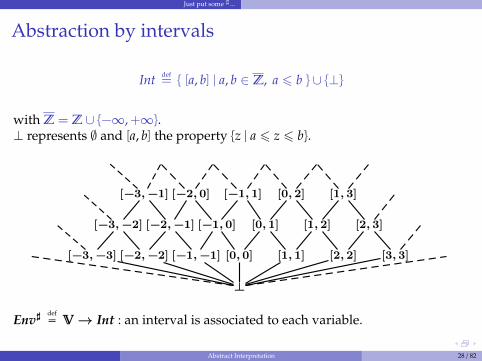
Abstraction by intervals
Int def= { [a, b] | a, b ∈ Z, a 6 b } ∪ {⊥}
with Z = Z ∪ {−∞,+∞}.⊥ represents ∅ and [a, b] the property {z | a 6 z 6 b}.Treillis de hauteur infinie (ex : intervalles)
[−3, −1] [−2, 0] [−1, 1] [0, 2] [1, 3]
[−3, −2] [−2, −1] [−1, 0] [0, 1] [1, 2] [2, 3]
[−3, −3] [−2, −2] [−1, −1] [0, 0] [1, 1] [2, 2] [3, 3]
⊥Dans un tel treillis, y0 = ⊥, yn+1 = F ](yn)ne converge pas necessairement en un nombre borne d’etapes.Exemple : analyse d’un compteur incremente indefiniment
Deux solutions
S’interdire de tels treillis abstraits ? Bien dommage !
Extrapoler la limite avec un op. d’elargissement ∇Idee : [−3, 3] ∇ [−5, 3] = [−∞, 3]
n n + 1 extrapolation
– p.6
Env] def= V→ Int : an interval is associated to each variable.
Abstract Interpretation 28 / 82
Just put some ] ...
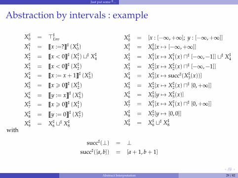
Abstraction by intervals : example
X]0 = >]
Env
X]1 = ~x :=?�] (X]
0)
X]2 = ~x < 0�] (X]
1) t] X]4
X]3 = ~x < 0�] (X]
2)
X]4 = ~x := x + 1�] (X]
3)
X]5 = ~x > 0�] (X]
2)
X]6 =
�
y := x�]
(X]5)
X]7 = ~x > 0�] (X]
1)
X]8 =
�
y := 0�]
(X]7)
X]9 = X]
6 t] X]8
X]0 = [x : [−∞,+∞]; y : [−∞,+∞]]
X]1 = X]
0[x 7→ [−∞,+∞]]
X]2 = X]
1[x 7→ X]1(x) u] [−∞,−1]] t] X]
4
X]3 = X]
2[x 7→ X]2(x) u] [−∞,−1]]
X]4 = X]
3[x 7→ succ](X]3(x))]
X]5 = X]
2[x 7→ X]2(x) u] [0,+∞]]
X]6 = X]
5[y 7→ X]5(x)]
X]7 = X]
1[x 7→ X]1(x) u] [0,+∞]]
X]8 = X]
7[y 7→ [0, 0]]
X]9 = X]
6 t] X]8
with
succ](⊥) = ⊥succ]([a, b]) = [a + 1, b + 1]
Abstract Interpretation 29 / 82
Demo
Building a generic abstract interpreter
Outline
1 Introduction
2 Intermediate representation : syntax and semantics
3 Collecting semantics
4 Just put some ]...
5 Building a generic abstract interpreter
6 Numeric abstraction by intervals
7 Widening/Narrowing
8 Polyhedral abstract interpretation
9 Readings
Abstract Interpretation 31 / 82
Building a generic abstract interpreter
Soundness criterion
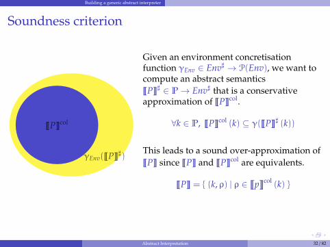
~P�col
γEnv(~P�])
Given an environment concretisationfunction γEnv ∈ Env] → P(Env), we want tocompute an abstract semantics~P�] ∈ P→ Env] that is a conservativeapproximation of ~P�col.
∀k ∈ P, ~P�col (k) ⊆ γ(~P�] (k))
This leads to a sound over-approximation of~P� since ~P� and ~P�col are equivalents.
~P� = { (k, ρ) | ρ ∈ �p�col (k) }
Abstract Interpretation 32 / 82
Building a generic abstract interpreter
Function approximation
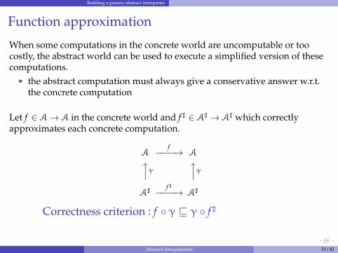
When some computations in the concrete world are uncomputable or toocostly, the abstract world can be used to execute a simplified version of thesecomputations.I the abstract computation must always give a conservative answer w.r.t.
the concrete computation
Let f ∈ A→ A in the concrete world and f ] ∈ A] → A] which correctlyapproximates each concrete computation.
Af−−−−→ A
xγxγ
A] f ]−−−−→ A]
Correctness criterion : f ◦ γ v γ ◦ f ]
Abstract Interpretation 33 / 82
Building a generic abstract interpreter
Fixpoint transfert
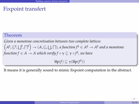
TheoremGiven a monotone concretisation between two complete lattices(A],v],
⊔],�])→ (A,v,
⊔,�
), a function f ] ∈ A] → A] and a monotone
function f ∈ A→ A which verify f ◦ γ v γ ◦ f ], we have
lfp(f ) v γ(lfp(f ]))
It means it is generally sound to mimic fixpoint computation in the abstract.
Abstract Interpretation 34 / 82
Building a generic abstract interpreter
Environment abstraction : sufficient elements
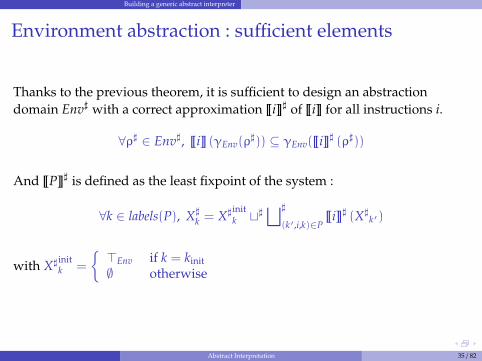
Thanks to the previous theorem, it is sufficient to design an abstractiondomain Env] with a correct approximation ~i�] of ~i� for all instructions i.
∀ρ] ∈ Env], ~i� (γEnv(ρ])) ⊆ γEnv(~i�] (ρ]))
And ~P�] is defined as the least fixpoint of the system :
∀k ∈ labels(P), X]k = X]init
k t]⊔]
(k′,i,k)∈P~i�] (X]
k′)
with X]initk =
{>Env if k = kinit∅ otherwise
Abstract Interpretation 35 / 82
Building a generic abstract interpreter
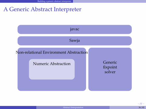
A Generic Abstract Interpreter
javac
Sawja
Non-relational Environment Abstraction
Numeric Abstraction Genericfixpointsolver
Abstract Interpretation 36 / 82
Building a generic abstract interpreter
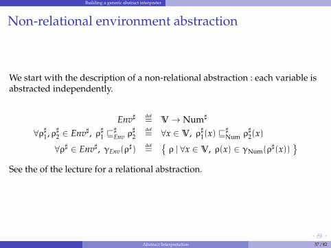
Non-relational environment abstraction
We start with the description of a non-relational abstraction : each variable isabstracted independently.
Env] def= V→ Num]
∀ρ]1, ρ]2 ∈ Env], ρ]1 v]Env ρ
]2
def= ∀x ∈ V, ρ]1(x) v
]Num ρ
]2(x)
∀ρ] ∈ Env], γEnv(ρ])
def={ρ | ∀x ∈ V, ρ(x) ∈ γNum(ρ
](x))}
See the of the lecture for a relational abstraction.
Abstract Interpretation 37 / 82
Building a generic abstract interpreter
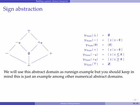
Sign abstraction
−0 +0
− 0 +
⊥
>γNum(⊥) = ∅γNum(−) = { z | z < 0 }
γNum(0) = {0}
γNum(+) = { z | z > 0 }
γNum(−0) = { z | z≤ 0 }
γNum(+0) = { z | z≥ 0 }
γNum(>) = Z
We will use this abstract domain as runnign example but you should keep inmind this is just an example among other numerical abstract domains.
Abstract Interpretation 38 / 82
Building a generic abstract interpreter
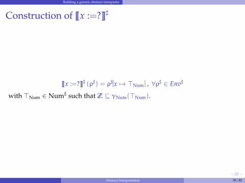
Construction of ~x :=?�]
~x :=?�] (ρ]) = ρ][x 7→ >Num] , ∀ρ] ∈ Env]
with >Num ∈ Num] such that Z ⊆ γNum(>Num).
Abstract Interpretation 39 / 82
Building a generic abstract interpreter
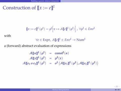
Construction of ~x := e�]
~x := e�] (ρ]) = ρ][x 7→ A~e�] (ρ])
], ∀ρ] ∈ Env]
with∀e ∈ Expr, A~e�] ∈ Env] → Num]
a (forward) abstract evaluation of expressions
A~n�] (ρ]) = const](n)A~x�] (ρ]) = ρ](x)
A~e1 o e2�] (ρ]) = o]
(A~e1�
] (ρ]),A~e2�] (ρ])
)
Abstract Interpretation 40 / 82
Building a generic abstract interpreter
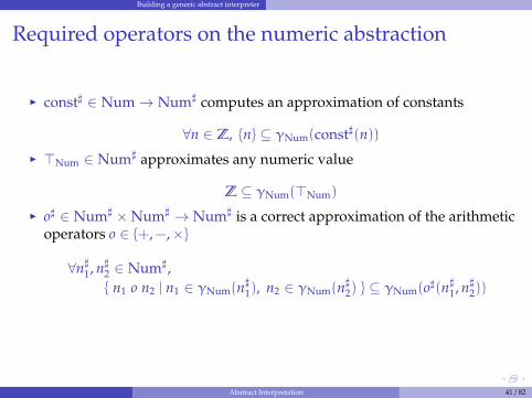
Required operators on the numeric abstraction
I const] ∈ Num→ Num] computes an approximation of constants
∀n ∈ Z, {n} ⊆ γNum(const](n))
I >Num ∈ Num] approximates any numeric value
Z ⊆ γNum(>Num)
I o] ∈ Num] ×Num] → Num] is a correct approximation of the arithmeticoperators o ∈ {+,−,×}
∀n]1, n]
2 ∈ Num],{ n1 o n2 | n1 ∈ γNum(n
]1), n2 ∈ γNum(n
]2) } ⊆ γNum(o](n
]1, n]
2))
Abstract Interpretation 41 / 82
Building a generic abstract interpreter
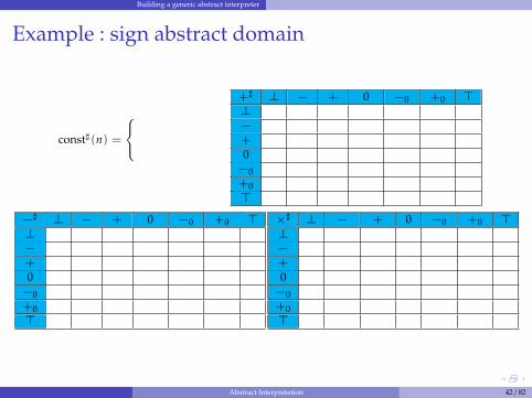
Example : sign abstract domain
const](n) =
+ if n > 00 if n = 0− if n < 0
+] ⊥ − + 0 −0 +0 >⊥
⊥ ⊥ ⊥ ⊥ ⊥ ⊥ ⊥
−
⊥ − > − − > >
+
⊥ > + + > + >
0
⊥ − + 0 −0 +0 >
−0
⊥ − > −0 −0 > >
+0
⊥ > + +0 > +0 >
>
⊥ > > > > > >
−] ⊥ − + 0 −0 +0 >⊥
⊥ ⊥ ⊥ ⊥ ⊥ ⊥ ⊥
−
⊥ > − − > − >
+
⊥ + > + + > >
0
⊥ + − 0 +0 −0 >
−0
⊥ > − −0 > −0 >
+0
⊥ + > +0 +0 > >
>
⊥ > > > > > >
×] ⊥ − + 0 −0 +0 >⊥
⊥ ⊥ ⊥ ⊥ ⊥ ⊥ ⊥
−
⊥ + + 0 +0 −0 >
+
⊥ − + 0 −0 +0 >
0
⊥ 0 0 0 0 0 0
−0
⊥ +0 −0 0 +0 −0 >
+0
⊥ −0 +0 0 −0 +0 >
>
⊥ > > 0 > > >
Abstract Interpretation 42 / 82
Building a generic abstract interpreter
Example : sign abstract domain
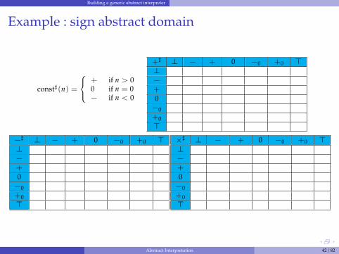
const](n) =
+ if n > 00 if n = 0− if n < 0
+] ⊥ − + 0 −0 +0 >⊥
⊥ ⊥ ⊥ ⊥ ⊥ ⊥ ⊥
−
⊥ − > − − > >
+
⊥ > + + > + >
0
⊥ − + 0 −0 +0 >
−0
⊥ − > −0 −0 > >
+0
⊥ > + +0 > +0 >
>
⊥ > > > > > >
−] ⊥ − + 0 −0 +0 >⊥
⊥ ⊥ ⊥ ⊥ ⊥ ⊥ ⊥
−
⊥ > − − > − >
+
⊥ + > + + > >
0
⊥ + − 0 +0 −0 >
−0
⊥ > − −0 > −0 >
+0
⊥ + > +0 +0 > >
>
⊥ > > > > > >
×] ⊥ − + 0 −0 +0 >⊥
⊥ ⊥ ⊥ ⊥ ⊥ ⊥ ⊥
−
⊥ + + 0 +0 −0 >
+
⊥ − + 0 −0 +0 >
0
⊥ 0 0 0 0 0 0
−0
⊥ +0 −0 0 +0 −0 >
+0
⊥ −0 +0 0 −0 +0 >
>
⊥ > > 0 > > >
Abstract Interpretation 42 / 82

Building a generic abstract interpreter
Example : sign abstract domain
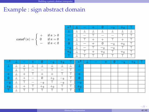
const](n) =
+ if n > 00 if n = 0− if n < 0
+] ⊥ − + 0 −0 +0 >⊥ ⊥ ⊥ ⊥ ⊥ ⊥ ⊥ ⊥− ⊥ − > − − > >+ ⊥ > + + > + >0 ⊥ − + 0 −0 +0 >−0 ⊥ − > −0 −0 > >+0 ⊥ > + +0 > +0 >> ⊥ > > > > > >
−] ⊥ − + 0 −0 +0 >⊥
⊥ ⊥ ⊥ ⊥ ⊥ ⊥ ⊥
−
⊥ > − − > − >
+
⊥ + > + + > >
0
⊥ + − 0 +0 −0 >
−0
⊥ > − −0 > −0 >
+0
⊥ + > +0 +0 > >
>
⊥ > > > > > >
×] ⊥ − + 0 −0 +0 >⊥
⊥ ⊥ ⊥ ⊥ ⊥ ⊥ ⊥
−
⊥ + + 0 +0 −0 >
+
⊥ − + 0 −0 +0 >
0
⊥ 0 0 0 0 0 0
−0
⊥ +0 −0 0 +0 −0 >
+0
⊥ −0 +0 0 −0 +0 >
>
⊥ > > 0 > > >
Abstract Interpretation 42 / 82
Building a generic abstract interpreter
Example : sign abstract domain
const](n) =
+ if n > 00 if n = 0− if n < 0
+] ⊥ − + 0 −0 +0 >⊥ ⊥ ⊥ ⊥ ⊥ ⊥ ⊥ ⊥− ⊥ − > − − > >+ ⊥ > + + > + >0 ⊥ − + 0 −0 +0 >−0 ⊥ − > −0 −0 > >+0 ⊥ > + +0 > +0 >> ⊥ > > > > > >
−] ⊥ − + 0 −0 +0 >⊥ ⊥ ⊥ ⊥ ⊥ ⊥ ⊥ ⊥− ⊥ > − − > − >+ ⊥ + > + + > >0 ⊥ + − 0 +0 −0 >−0 ⊥ > − −0 > −0 >+0 ⊥ + > +0 +0 > >> ⊥ > > > > > >
×] ⊥ − + 0 −0 +0 >⊥
⊥ ⊥ ⊥ ⊥ ⊥ ⊥ ⊥
−
⊥ + + 0 +0 −0 >
+
⊥ − + 0 −0 +0 >
0
⊥ 0 0 0 0 0 0
−0
⊥ +0 −0 0 +0 −0 >
+0
⊥ −0 +0 0 −0 +0 >
>
⊥ > > 0 > > >
Abstract Interpretation 42 / 82

Building a generic abstract interpreter
Example : sign abstract domain
const](n) =
+ if n > 00 if n = 0− if n < 0
+] ⊥ − + 0 −0 +0 >⊥ ⊥ ⊥ ⊥ ⊥ ⊥ ⊥ ⊥− ⊥ − > − − > >+ ⊥ > + + > + >0 ⊥ − + 0 −0 +0 >−0 ⊥ − > −0 −0 > >+0 ⊥ > + +0 > +0 >> ⊥ > > > > > >
−] ⊥ − + 0 −0 +0 >⊥ ⊥ ⊥ ⊥ ⊥ ⊥ ⊥ ⊥− ⊥ > − − > − >+ ⊥ + > + + > >0 ⊥ + − 0 +0 −0 >−0 ⊥ > − −0 > −0 >+0 ⊥ + > +0 +0 > >> ⊥ > > > > > >
×] ⊥ − + 0 −0 +0 >⊥ ⊥ ⊥ ⊥ ⊥ ⊥ ⊥ ⊥− ⊥ + + 0 +0 −0 >+ ⊥ − + 0 −0 +0 >0 ⊥ 0 0 0 0 0 0−0 ⊥ +0 −0 0 +0 −0 >+0 ⊥ −0 +0 0 −0 +0 >> ⊥ > > 0 > > >
Abstract Interpretation 42 / 82
Building a generic abstract interpreter
Construction of ~t�]
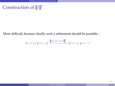
More difficult, because ideally such a refinement should be possible...
[x 7→ +; y 7→ −0]~(0−y)−x>0�
]
−−−−−−−−−→ [x 7→ +; y 7→ −]
Abstract Interpretation 43 / 82
Building a generic abstract interpreter
Construction of ~t�]
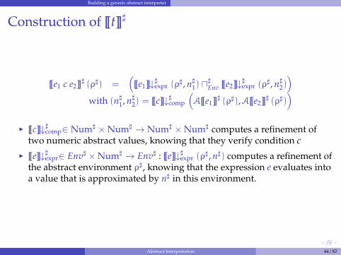
~e1 c e2�] (ρ]) =
(~e1�↓]expr (ρ
], n]1) u
]Env ~e2�↓]expr (ρ
], n]2))
with (n]1, n]
2) = ~c�↓]comp
(A~e1�
] (ρ]),A~e2�] (ρ])
)
I ~c�↓]comp∈ Num] ×Num] → Num] ×Num] computes a refinement oftwo numeric abstract values, knowing that they verify condition c
I ~e�↓]expr∈ Env] ×Num] → Env] : ~e�↓]expr (ρ], n]) computes a refinement of
the abstract environment ρ], knowing that the expression e evaluates intoa value that is approximated by n] in this environment.
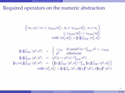
Abstract Interpretation 44 / 82
Building a generic abstract interpreter
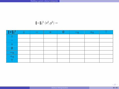
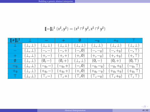
~=�↓] (x], y]) =
(x] u] y], x] u] y])
~,�↓] ⊥ − + 0 −0 +0 >⊥
(⊥,⊥) (⊥,⊥) (⊥,⊥) (⊥,⊥) (⊥,⊥) (⊥,⊥) (⊥,⊥)
−
(⊥,⊥) (−,−) (−,+) (−, 0) (−,−0) (−,+0) (−,>)
+
(⊥,⊥) (+,−) (+,+) (+, 0) (+,−0) (+,+0) (+,>)
0
(⊥,⊥) (0,−) (0,+) (⊥,⊥) (0,−) (0,+) (0,>)
−0
(⊥,⊥) (−0,−) (−0,+) (−, 0) (−0,−0) (−0,+0) (−0,>)
+0
(⊥,⊥) (+0,−) (+0,+) (+, 0) (+0,−0) (+0,+0) (+0,>)
>
(⊥,⊥) (>,−) (>,+) (>, 0) (>,−0) (>,+0) (>,>)
Abstract Interpretation 45 / 82
Building a generic abstract interpreter
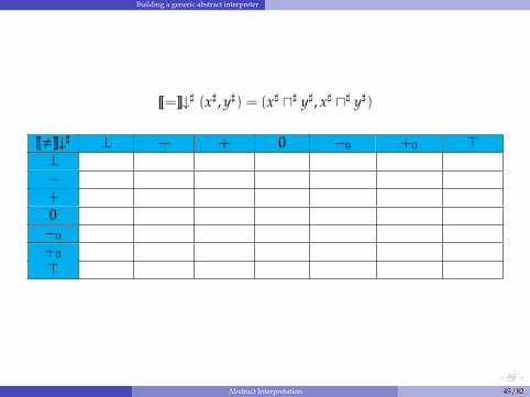
~=�↓] (x], y]) = (x] u] y], x] u] y])
~,�↓] ⊥ − + 0 −0 +0 >⊥
(⊥,⊥) (⊥,⊥) (⊥,⊥) (⊥,⊥) (⊥,⊥) (⊥,⊥) (⊥,⊥)
−
(⊥,⊥) (−,−) (−,+) (−, 0) (−,−0) (−,+0) (−,>)
+
(⊥,⊥) (+,−) (+,+) (+, 0) (+,−0) (+,+0) (+,>)
0
(⊥,⊥) (0,−) (0,+) (⊥,⊥) (0,−) (0,+) (0,>)
−0
(⊥,⊥) (−0,−) (−0,+) (−, 0) (−0,−0) (−0,+0) (−0,>)
+0
(⊥,⊥) (+0,−) (+0,+) (+, 0) (+0,−0) (+0,+0) (+0,>)
>
(⊥,⊥) (>,−) (>,+) (>, 0) (>,−0) (>,+0) (>,>)
Abstract Interpretation 45 / 82
Building a generic abstract interpreter
~=�↓] (x], y]) = (x] u] y], x] u] y])
~,�↓] ⊥ − + 0 −0 +0 >⊥ (⊥,⊥) (⊥,⊥) (⊥,⊥) (⊥,⊥) (⊥,⊥) (⊥,⊥) (⊥,⊥)− (⊥,⊥) (−,−) (−,+) (−, 0) (−,−0) (−,+0) (−,>)+ (⊥,⊥) (+,−) (+,+) (+, 0) (+,−0) (+,+0) (+,>)0 (⊥,⊥) (0,−) (0,+) (⊥,⊥) (0,−) (0,+) (0,>)−0 (⊥,⊥) (−0,−) (−0,+) (−, 0) (−0,−0) (−0,+0) (−0,>)+0 (⊥,⊥) (+0,−) (+0,+) (+, 0) (+0,−0) (+0,+0) (+0,>)> (⊥,⊥) (>,−) (>,+) (>, 0) (>,−0) (>,+0) (>,>)
Abstract Interpretation 45 / 82
Building a generic abstract interpreter
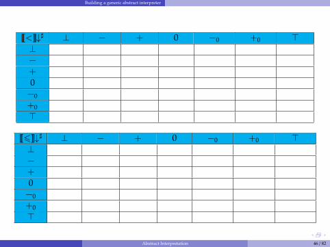
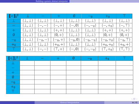
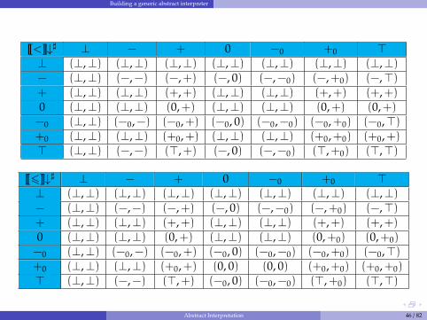
~<�↓] ⊥ − + 0 −0 +0 >⊥
(⊥,⊥) (⊥,⊥) (⊥,⊥) (⊥,⊥) (⊥,⊥) (⊥,⊥) (⊥,⊥)
−
(⊥,⊥) (−,−) (−,+) (−, 0) (−,−0) (−,+0) (−,>)
+
(⊥,⊥) (⊥,⊥) (+,+) (⊥,⊥) (⊥,⊥) (+,+) (+,+)
0
(⊥,⊥) (⊥,⊥) (0,+) (⊥,⊥) (⊥,⊥) (0,+) (0,+)
−0
(⊥,⊥) (−0,−) (−0,+) (−0, 0) (−0,−0) (−0,+0) (−0,>)
+0
(⊥,⊥) (⊥,⊥) (+0,+) (⊥,⊥) (⊥,⊥) (+0,+0) (+0,+)
>
(⊥,⊥) (−,−) (>,+) (−, 0) (−,−0) (>,+0) (>,>)
~6�↓] ⊥ − + 0 −0 +0 >⊥
(⊥,⊥) (⊥,⊥) (⊥,⊥) (⊥,⊥) (⊥,⊥) (⊥,⊥) (⊥,⊥)
−
(⊥,⊥) (−,−) (−,+) (−, 0) (−,−0) (−,+0) (−,>)
+
(⊥,⊥) (⊥,⊥) (+,+) (⊥,⊥) (⊥,⊥) (+,+) (+,+)
0
(⊥,⊥) (⊥,⊥) (0,+) (⊥,⊥) (⊥,⊥) (0,+0) (0,+0)
−0
(⊥,⊥) (−0,−) (−0,+) (−0, 0) (−0,−0) (−0,+0) (−0,>)
+0
(⊥,⊥) (⊥,⊥) (+0,+) (0, 0) (0, 0) (+0,+0) (+0,+0)
>
(⊥,⊥) (−,−) (>,+) (−0, 0) (−0,−0) (>,+0) (>,>)
Abstract Interpretation 46 / 82
Building a generic abstract interpreter
~<�↓] ⊥ − + 0 −0 +0 >⊥ (⊥,⊥) (⊥,⊥) (⊥,⊥) (⊥,⊥) (⊥,⊥) (⊥,⊥) (⊥,⊥)− (⊥,⊥) (−,−) (−,+) (−, 0) (−,−0) (−,+0) (−,>)+ (⊥,⊥) (⊥,⊥) (+,+) (⊥,⊥) (⊥,⊥) (+,+) (+,+)0 (⊥,⊥) (⊥,⊥) (0,+) (⊥,⊥) (⊥,⊥) (0,+) (0,+)−0 (⊥,⊥) (−0,−) (−0,+) (−0, 0) (−0,−0) (−0,+0) (−0,>)+0 (⊥,⊥) (⊥,⊥) (+0,+) (⊥,⊥) (⊥,⊥) (+0,+0) (+0,+)> (⊥,⊥) (−,−) (>,+) (−, 0) (−,−0) (>,+0) (>,>)
~6�↓] ⊥ − + 0 −0 +0 >⊥ (⊥,⊥) (⊥,⊥) (⊥,⊥) (⊥,⊥) (⊥,⊥) (⊥,⊥) (⊥,⊥)− (⊥,⊥) (−,−) (−,+) (−, 0) (−,−0) (−,+0) (−,>)+ (⊥,⊥) (⊥,⊥) (+,+) (⊥,⊥) (⊥,⊥) (+,+) (+,+)0 (⊥,⊥) (⊥,⊥) (0,+) (⊥,⊥) (⊥,⊥) (0,+0) (0,+0)−0 (⊥,⊥) (−0,−) (−0,+) (−0, 0) (−0,−0) (−0,+0) (−0,>)+0 (⊥,⊥) (⊥,⊥) (+0,+) (0, 0) (0, 0) (+0,+0) (+0,+0)> (⊥,⊥) (−,−) (>,+) (−0, 0) (−0,−0) (>,+0) (>,>)
Abstract Interpretation 46 / 82
Building a generic abstract interpreter
Required operators on the numeric abstraction
{(n1, n2) | n1 ∈ γNum(n
]1), n2 ∈ γNum(n
]2), n1 c n2
}⊆ γNum(m
]1)× γNum(m
]2)
with (m]1, m]
2) = ~c�↓]comp (n]
1, n]2)
~n�↓]expr (ρ], n]) =
{⊥Env if const](n) u]Num n] = ⊥Numρ] otherwise
~x�↓]expr (ρ], n]) = (ρ][x 7→ ρ](x) u]Num n]])
~e1 o e2�↓]expr (ρ], n]) =
(~e1�↓]expr (ρ
], n]1) u
]Env ~e2�↓]expr (ρ
], n]2))
with (n]1, n]
2) = ~o�↓]op (n],A~e1�
] (ρ]),A~e2�] (ρ]))
Abstract Interpretation 47 / 82
Building a generic abstract interpreter
Required operators on the numeric abstraction
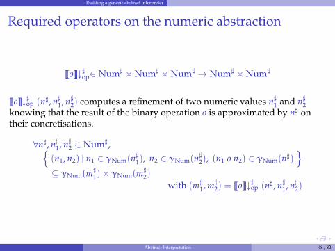
~o�↓]op∈ Num] ×Num] ×Num] → Num] ×Num]
~o�↓]op (n], n]1, n]
2) computes a refinement of two numeric values n]1 and n]
2knowing that the result of the binary operation o is approximated by n] ontheir concretisations.
∀n], n]1, n]
2 ∈ Num],{(n1, n2) | n1 ∈ γNum(n
]1), n2 ∈ γNum(n
]2), (n1 o n2) ∈ γNum(n])
}⊆ γNum(m
]1)× γNum(m
]2)
with (m]1, m]
2) = ~o�↓]op (n], n]
1, n]2)
Abstract Interpretation 48 / 82
Building a generic abstract interpreter
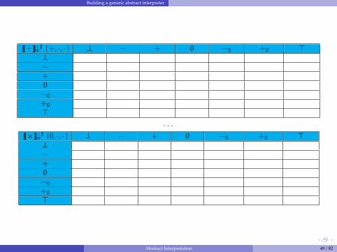
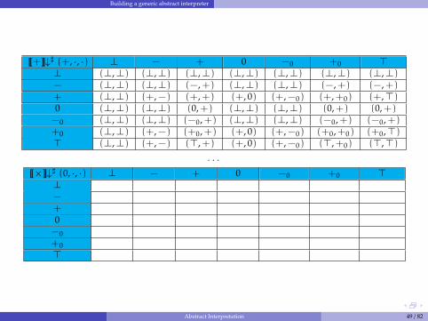
~+�↓] (+, ·, ·) ⊥ − + 0 −0 +0 >⊥
(⊥,⊥) (⊥,⊥) (⊥,⊥) (⊥,⊥) (⊥,⊥) (⊥,⊥) (⊥,⊥)
−
(⊥,⊥) (⊥,⊥) (−,+) (⊥,⊥) (⊥,⊥) (−,+) (−,+)
+
(⊥,⊥) (+,−) (+,+) (+, 0) (+,−0) (+,+0) (+,>)
0
(⊥,⊥) (⊥,⊥) (0,+) (⊥,⊥) (⊥,⊥) (0,+) (0,+)
−0
(⊥,⊥) (⊥,⊥) (−0,+) (⊥,⊥) (⊥,⊥) (−0,+) (−0,+)
+0
(⊥,⊥) (+,−) (+0,+) (+, 0) (+,−0) (+0,+0) (+0,>)
>
(⊥,⊥) (+,−) (>,+) (+, 0) (+,−0) (>,+0) (>,>)
· · ·~×�↓] (0, ·, ·) ⊥ − + 0 −0 +0 >
⊥
(⊥,⊥) (⊥,⊥) (⊥,⊥) (⊥,⊥) (⊥,⊥) (⊥,⊥) (⊥,⊥)
−
(⊥,⊥) (⊥,⊥) (⊥,⊥) (−, 0) (−, 0) (−, 0) (−, 0)
+
(⊥,⊥) (⊥,⊥) (⊥,⊥) (+, 0) (+, 0) (+, 0) (+, 0)
0
(⊥,⊥) (0, ) (0,+) (0, 0) (0,−0) (0,+0) (0,>)
−0
(⊥,⊥) (0,−) (0,+) (−0, 0) (−0,−0) (−0,+0) (−0,>)
+0
(⊥,⊥) (0,−) (0,+) (+0, 0) (+0,−0) (+0,+0) (+0,>)
>
(⊥,⊥) (0,−) (0,+) (>, 0) (>, 0) (>, 0) (>,>)
Abstract Interpretation 49 / 82
Building a generic abstract interpreter
~+�↓] (+, ·, ·) ⊥ − + 0 −0 +0 >⊥ (⊥,⊥) (⊥,⊥) (⊥,⊥) (⊥,⊥) (⊥,⊥) (⊥,⊥) (⊥,⊥)− (⊥,⊥) (⊥,⊥) (−,+) (⊥,⊥) (⊥,⊥) (−,+) (−,+)+ (⊥,⊥) (+,−) (+,+) (+, 0) (+,−0) (+,+0) (+,>)0 (⊥,⊥) (⊥,⊥) (0,+) (⊥,⊥) (⊥,⊥) (0,+) (0,+)−0 (⊥,⊥) (⊥,⊥) (−0,+) (⊥,⊥) (⊥,⊥) (−0,+) (−0,+)+0 (⊥,⊥) (+,−) (+0,+) (+, 0) (+,−0) (+0,+0) (+0,>)> (⊥,⊥) (+,−) (>,+) (+, 0) (+,−0) (>,+0) (>,>)
· · ·~×�↓] (0, ·, ·) ⊥ − + 0 −0 +0 >
⊥ (⊥,⊥) (⊥,⊥) (⊥,⊥) (⊥,⊥) (⊥,⊥) (⊥,⊥) (⊥,⊥)− (⊥,⊥) (⊥,⊥) (⊥,⊥) (−, 0) (−, 0) (−, 0) (−, 0)+ (⊥,⊥) (⊥,⊥) (⊥,⊥) (+, 0) (+, 0) (+, 0) (+, 0)0 (⊥,⊥) (0, ) (0,+) (0, 0) (0,−0) (0,+0) (0,>)−0 (⊥,⊥) (0,−) (0,+) (−0, 0) (−0,−0) (−0,+0) (−0,>)+0 (⊥,⊥) (0,−) (0,+) (+0, 0) (+0,−0) (+0,+0) (+0,>)> (⊥,⊥) (0,−) (0,+) (>, 0) (>, 0) (>, 0) (>,>)
Abstract Interpretation 49 / 82
Building a generic abstract interpreter
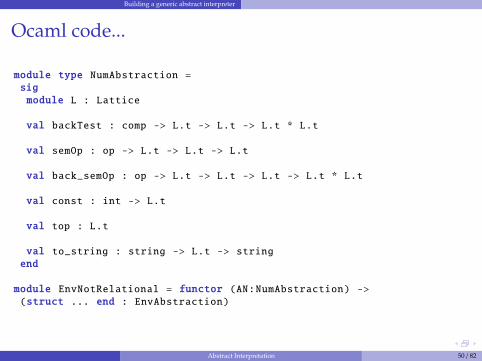
Ocaml code...
module type NumAbstraction =sigmodule L : Lattice
val backTest : comp -> L.t -> L.t -> L.t * L.t
val semOp : op -> L.t -> L.t -> L.t
val back_semOp : op -> L.t -> L.t -> L.t -> L.t * L.t
val const : int -> L.t
val top : L.t
val to_string : string -> L.t -> stringend
module EnvNotRelational = functor (AN:NumAbstraction) ->(struct ... end : EnvAbstraction)
Abstract Interpretation 50 / 82
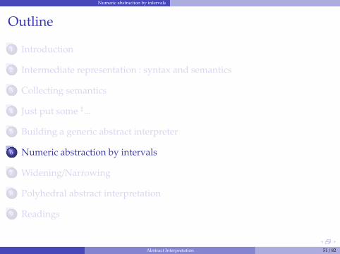
Numeric abstraction by intervals
Outline
1 Introduction
2 Intermediate representation : syntax and semantics
3 Collecting semantics
4 Just put some ]...
5 Building a generic abstract interpreter
6 Numeric abstraction by intervals
7 Widening/Narrowing
8 Polyhedral abstract interpretation
9 Readings
Abstract Interpretation 51 / 82
Numeric abstraction by intervals
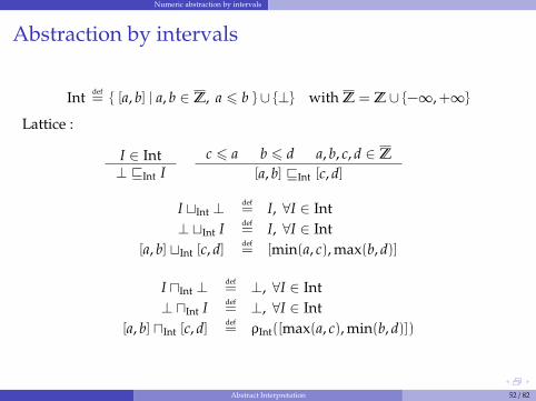
Abstraction by intervals
Int def= { [a, b] | a, b ∈ Z, a 6 b } ∪ {⊥} with Z = Z ∪ {−∞,+∞}
Lattice :
I ∈ Int⊥ vInt I
c 6 a b 6 d a, b, c, d ∈ Z[a, b] vInt [c, d]
I tInt ⊥ def= I, ∀I ∈ Int
⊥ tInt I def= I, ∀I ∈ Int
[a, b] tInt [c, d] def= [min(a, c), max(b, d)]
I uInt ⊥ def= ⊥, ∀I ∈ Int
⊥ uInt I def= ⊥, ∀I ∈ Int
[a, b] uInt [c, d] def= ρInt([max(a, c), min(b, d)])
Abstract Interpretation 52 / 82
Numeric abstraction by intervals
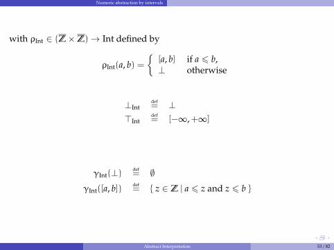
with ρInt ∈ (Z×Z)→ Int defined by
ρInt(a, b) ={
[a, b] if a 6 b,⊥ otherwise
⊥Intdef= ⊥
>Intdef= [−∞,+∞]
γInt(⊥) def= ∅
γInt([a, b]) def= { z ∈ Z | a 6 z and z 6 b }
Abstract Interpretation 53 / 82
Numeric abstraction by intervals
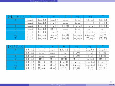
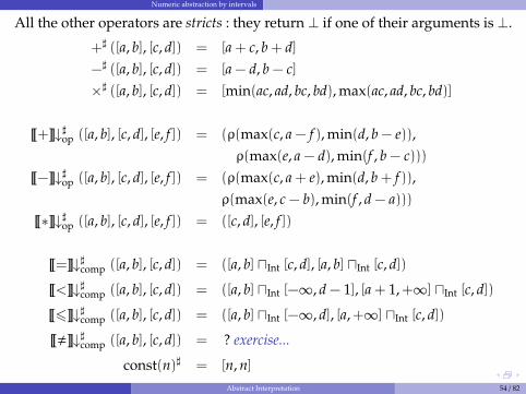
All the other operators are stricts : they return ⊥ if one of their arguments is ⊥.
+] ([a, b], [c, d]) = [a + c, b + d]−] ([a, b], [c, d]) = [a − d, b − c]×] ([a, b], [c, d]) = [min(ac, ad, bc, bd), max(ac, ad, bc, bd)]
~+�↓]op ([a, b], [c, d], [e, f ]) = (ρ(max(c, a − f ), min(d, b − e)),ρ(max(e, a − d), min(f , b − c)))
~−�↓]op ([a, b], [c, d], [e, f ]) = (ρ(max(c, a + e), min(d, b + f )),ρ(max(e, c − b), min(f , d − a)))
~∗�↓]op ([a, b], [c, d], [e, f ]) = ([c, d], [e, f ])
~=�↓]comp ([a, b], [c, d]) = ([a, b] uInt [c, d], [a, b] uInt [c, d])
~<�↓]comp ([a, b], [c, d]) = ([a, b] uInt [−∞, d − 1], [a + 1,+∞] uInt [c, d])
~6�↓]comp ([a, b], [c, d]) = ([a, b] uInt [−∞, d], [a,+∞] uInt [c, d])
~,�↓]comp ([a, b], [c, d]) = ? exercise...
const(n)] = [n, n]Abstract Interpretation 54 / 82
Numeric abstraction by intervals
Convergence problemTreillis de hauteur infinie (ex : intervalles)
[−3, −1] [−2, 0] [−1, 1] [0, 2] [1, 3]
[−3, −2] [−2, −1] [−1, 0] [0, 1] [1, 2] [2, 3]
[−3, −3] [−2, −2] [−1, −1] [0, 0] [1, 1] [2, 2] [3, 3]
⊥Dans un tel treillis, y0 = ⊥, yn+1 = F ](yn)ne converge pas necessairement en un nombre borne d’etapes.Exemple : analyse d’un compteur incremente indefiniment
Deux solutions
S’interdire de tels treillis abstraits ? Bien dommage !
Extrapoler la limite avec un op. d’elargissement ∇Idee : [−3, 3] ∇ [−5, 3] = [−∞, 3]
n n + 1 extrapolation
– p.6
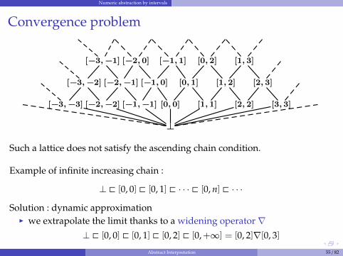
Such a lattice does not satisfy the ascending chain condition.
Example of infinite increasing chain :
⊥ @ [0, 0] @ [0, 1] @ · · · @ [0, n] @ · · ·
Solution : dynamic approximationI we extrapolate the limit thanks to a widening operator∇
⊥ @ [0, 0] @ [0, 1] @ [0, 2] @ [0,+∞] = [0, 2]∇[0, 3]
Abstract Interpretation 55 / 82
Widening/Narrowing
Outline
1 Introduction
2 Intermediate representation : syntax and semantics
3 Collecting semantics
4 Just put some ]...
5 Building a generic abstract interpreter
6 Numeric abstraction by intervals
7 Widening/Narrowing
8 Polyhedral abstract interpretation
9 Readings
Abstract Interpretation 56 / 82
Widening/Narrowing
Fixpoint approximation
LemmaLet (A,v,t,u) a complete lattice and f a monotone operator on A. If a is apost-fixpoint of f (i.e. f (a) v a), then lfp(f ) v a.
We may want to compute an over-approximation of lfp(f ) in the followingcases :I The lattice does not satisfies the ascending chain condition, the iteration⊥, f (⊥), . . . , f n(⊥), . . . may never terminates.
I The ascending chain condition is satisfied but the iteration chain is toolong to allow an efficient computation.
I Id the underlying lattice is not complete, the limits of the ascendingiterations do not necessarily belongs to the abstraction domain.
Abstract Interpretation 57 / 82
Widening/Narrowing
Widening
Idea : the standard iteration is of the form
x0 = ⊥, xn+1 = F(xn) = xn t F(xn)
We will replace it by something of the form
y0 = ⊥, yn+1 = yn∇F(yn)
such that(i) (yn) is increasing,
(ii) xn v yn, for all n,(iii) and (yn) stabilizes after a finite number of steps.But we also want a∇ operator that is independent of F.
Abstract Interpretation 58 / 82
Widening/Narrowing
Widening : definition
A widening is an operator∇ : L× L→ L such thatI ∀x, x ′ ∈ L, x t x ′ v x∇x ′ (implies (i) & (ii))I If x0 v x1 v . . . is an increasing chain, then the increasing chain
y0 = x0, yn+1 = yn∇xn+1 stabilizes after a finite number of steps (implies(iii)).
Usage : we replace x0 = ⊥, xn+1 = F(xn)by y0 = ⊥, yn+1 = yn∇F(yn)
Abstract Interpretation 59 / 82
Widening/Narrowing
Widening : theorem
TheoremLet L a complete lattice, F : L→ L a monotone function and∇ : L× L→ L awidening operator. The chain y0 = ⊥, yn+1 = yn∇F(yn) stabilizes after a finitenumber of steps towards a post-fixpoint y of F.
Corollary : lfp(F) v y.
Abstract Interpretation 60 / 82
Widening/Narrowing
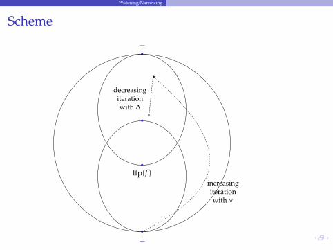
Scheme
⊥
>
lfp(f )increasingiterationwith O
decreasingiterationwith ∆
Abstract Interpretation 61 / 82
Widening/Narrowing
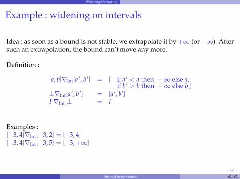
Example : widening on intervals
Idea : as soon as a bound is not stable, we extrapolate it by +∞ (or −∞). Aftersuch an extrapolation, the bound can’t move any more.
Definition :
[a, b]∇Int[a ′, b ′] = [ if a ′ < a then −∞ else a,if b ′ > b then +∞ else b ]
⊥∇Int[a ′, b ′] = [a ′, b ′]I ∇Int ⊥ = I
Examples :[−3, 4]∇Int[−3, 2] = [−3, 4][−3, 4]∇Int[−3, 5] = [−3,+∞]
Abstract Interpretation 62 / 82
Widening/Narrowing
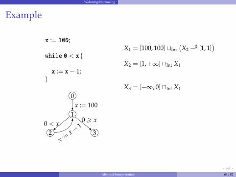
Example
x := 100;
while 0 < x {
x := x− 1;}
0
1
2 3
x := 100
0 < x
x :=x−
10 > x
X1 = [100, 100] tInt(X2 −
] [1, 1])
X2 = [1,+∞] uInt X1
X3 = [−∞, 0] uInt X1
Abstract Interpretation 63 / 82
Widening/Narrowing
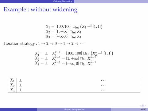
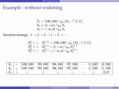
Example : without widening
X1 = [100, 100] tInt(X2 −
] [1, 1])
X2 = [1,+∞] uInt X1X3 = [−∞, 0] uInt X1
Iteration strategy : 1→ 2→ 3→ 1→ 2→ · · ·
X01 = ⊥
X02 = ⊥
X03 = ⊥
Xn+11 = [100, 100] tInt
(Xn
2 −] [1, 1])
Xn+12 = [1,+∞] uInt Xn+1
1Xn+1
3 = [−∞, 0] uInt Xn+11
X1 ⊥
[100, 100] [99, 100] [98, 100] [97, 100]
· · ·
[1, 100] [0, 100]
X2 ⊥
[100, 100] [99, 100] [98, 100] [97, 100]
· · ·
[1, 100] [1, 100]
X3 ⊥
⊥ ⊥ ⊥ ⊥
· · ·
⊥ [0, 0]
Abstract Interpretation 64 / 82
Widening/Narrowing
Example : without widening
X1 = [100, 100] tInt(X2 −
] [1, 1])
X2 = [1,+∞] uInt X1X3 = [−∞, 0] uInt X1
Iteration strategy : 1→ 2→ 3→ 1→ 2→ · · ·
X01 = ⊥
X02 = ⊥
X03 = ⊥
Xn+11 = [100, 100] tInt
(Xn
2 −] [1, 1])
Xn+12 = [1,+∞] uInt Xn+1
1Xn+1
3 = [−∞, 0] uInt Xn+11
X1 ⊥ [100, 100] [99, 100] [98, 100] [97, 100] · · · [1, 100] [0, 100]X2 ⊥ [100, 100] [99, 100] [98, 100] [97, 100] · · · [1, 100] [1, 100]X3 ⊥ ⊥ ⊥ ⊥ ⊥ · · · ⊥ [0, 0]
Abstract Interpretation 64 / 82
Widening/Narrowing
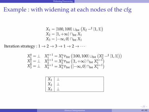
Example : with widening at each nodes of the cfg
X1 = [100, 100] tInt(X2 −
] [1, 1])
X2 = [1,+∞] uInt X1X3 = [−∞, 0] uInt X1
Iteration strategy : 1→ 2→ 3→ 1→ 2→ · · ·
X01 = ⊥
X02 = ⊥
X03 = ⊥
Xn+11 = Xn
1OInt([100, 100] tInt
(Xn
2 −] [1, 1]))
Xn+12 = Xn
2OInt([1,+∞] uInt Xn+1
1
)
Xn+13 = Xn
3OInt([−∞, 0] uInt Xn+1
1
)
X1 ⊥
[100, 100] [−∞, 100]
X2 ⊥
[100, 100] [−∞, 100]
X3 ⊥
⊥ [−∞, 0]
Abstract Interpretation 65 / 82
Widening/Narrowing
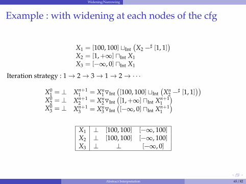
Example : with widening at each nodes of the cfg
X1 = [100, 100] tInt(X2 −
] [1, 1])
X2 = [1,+∞] uInt X1X3 = [−∞, 0] uInt X1
Iteration strategy : 1→ 2→ 3→ 1→ 2→ · · ·
X01 = ⊥
X02 = ⊥
X03 = ⊥
Xn+11 = Xn
1OInt([100, 100] tInt
(Xn
2 −] [1, 1]))
Xn+12 = Xn
2OInt([1,+∞] uInt Xn+1
1
)
Xn+13 = Xn
3OInt([−∞, 0] uInt Xn+1
1
)
X1 ⊥ [100, 100] [−∞, 100]X2 ⊥ [100, 100] [−∞, 100]X3 ⊥ ⊥ [−∞, 0]
Abstract Interpretation 65 / 82
Widening/Narrowing
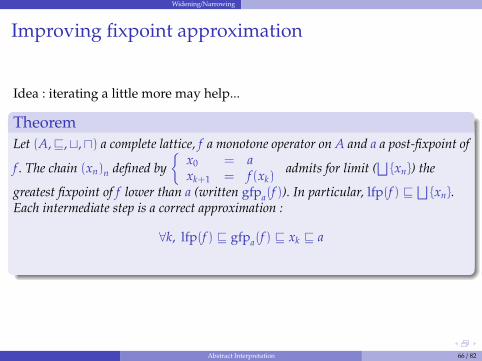
Improving fixpoint approximation
Idea : iterating a little more may help...
TheoremLet (A,v,t,u) a complete lattice, f a monotone operator on A and a a post-fixpoint of
f . The chain (xn)n defined by{
x0 = axk+1 = f (xk)
admits for limit (⊔{xn}) the
greatest fixpoint of f lower than a (written gfpa(f )). In particular, lfp(f ) v ⊔ {xn}.Each intermediate step is a correct approximation :
∀k, lfp(f ) v gfpa(f ) v xk v a
Abstract Interpretation 66 / 82
Widening/Narrowing
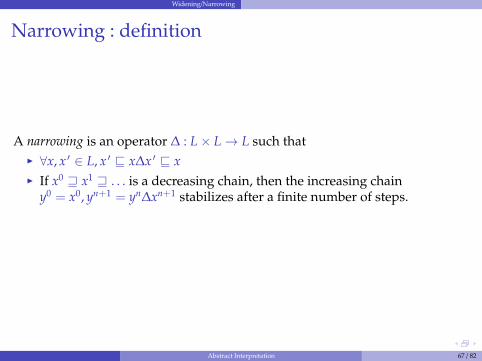
Narrowing : definition
A narrowing is an operator ∆ : L× L→ L such thatI ∀x, x ′ ∈ L, x ′ v x∆x ′ v xI If x0 w x1 w . . . is a decreasing chain, then the increasing chain
y0 = x0, yn+1 = yn∆xn+1 stabilizes after a finite number of steps.
Abstract Interpretation 67 / 82
Widening/Narrowing
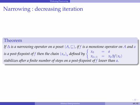
Narrowing : decreasing iteration
TheoremIf ∆ is a narrowing operator on a poset (A,v), if f is a monotone operator on A and a
is a post-fixpoint of f then the chain (xn)n defined by{
x0 = axk+1 = xk∆f (xk)
stabilizes after a finite number of steps on a post-fixpoint of f lower than a.
Abstract Interpretation 68 / 82
Widening/Narrowing
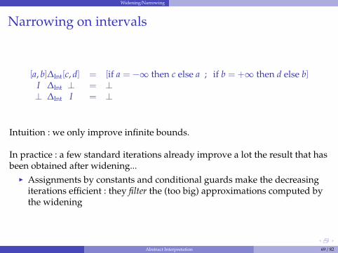
Narrowing on intervals
[a, b]∆Int[c, d] = [if a = −∞ then c else a ; if b = +∞ then d else b]I ∆Int ⊥ = ⊥⊥ ∆Int I = ⊥
Intuition : we only improve infinite bounds.
In practice : a few standard iterations already improve a lot the result that hasbeen obtained after widening...I Assignments by constants and conditional guards make the decreasing
iterations efficient : they filter the (too big) approximations computed bythe widening
Abstract Interpretation 69 / 82
Widening/Narrowing
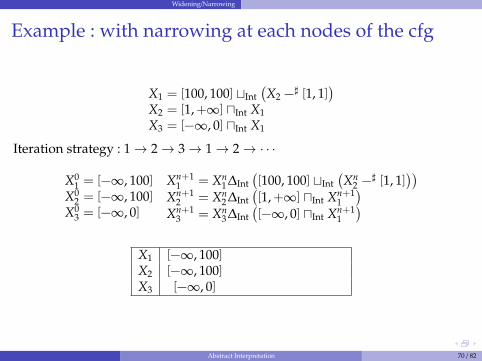
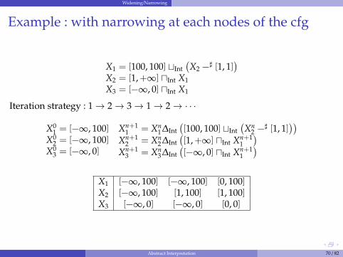
Example : with narrowing at each nodes of the cfg
X1 = [100, 100] tInt(X2 −
] [1, 1])
X2 = [1,+∞] uInt X1X3 = [−∞, 0] uInt X1
Iteration strategy : 1→ 2→ 3→ 1→ 2→ · · ·
X01 = [−∞, 100]
X02 = [−∞, 100]
X03 = [−∞, 0]
Xn+11 = Xn
1∆Int([100, 100] tInt
(Xn
2 −] [1, 1]))
Xn+12 = Xn
2∆Int([1,+∞] uInt Xn+1
1
)
Xn+13 = Xn
3∆Int([−∞, 0] uInt Xn+1
1
)
X1 [−∞, 100]
[−∞, 100] [0, 100]
X2 [−∞, 100]
[1, 100] [1, 100]
X3 [−∞, 0]
[−∞, 0] [0, 0]
Abstract Interpretation 70 / 82
Widening/Narrowing
Example : with narrowing at each nodes of the cfg
X1 = [100, 100] tInt(X2 −
] [1, 1])
X2 = [1,+∞] uInt X1X3 = [−∞, 0] uInt X1
Iteration strategy : 1→ 2→ 3→ 1→ 2→ · · ·
X01 = [−∞, 100]
X02 = [−∞, 100]
X03 = [−∞, 0]
Xn+11 = Xn
1∆Int([100, 100] tInt
(Xn
2 −] [1, 1]))
Xn+12 = Xn
2∆Int([1,+∞] uInt Xn+1
1
)
Xn+13 = Xn
3∆Int([−∞, 0] uInt Xn+1
1
)
X1 [−∞, 100] [−∞, 100] [0, 100]X2 [−∞, 100] [1, 100] [1, 100]X3 [−∞, 0] [−∞, 0] [0, 0]
Abstract Interpretation 70 / 82
Widening/Narrowing
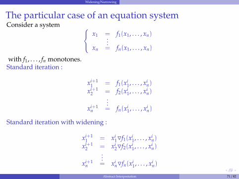
The particular case of an equation systemConsider a system x1 = f1(x1, . . . , xn)...
xn = fn(x1, . . . , xn)
with f1, . . . , fn monotones.Standard iteration :
xi+11 = f1(xi
1, . . . , xin)
xi+12 = f2(xi
1, . . . , xin)
...xi+1
n = fn(xi1, . . . , xi
n)
Standard iteration with widening :
xi+11 = xi
1Of1(xi1, . . . , xi
n)
xi+12 = xi
2Of2(xi1, . . . , xi
n)...
xi+1n = xi
nOfn(xi1, . . . , xi
n)
Abstract Interpretation 71 / 82
Widening/Narrowing
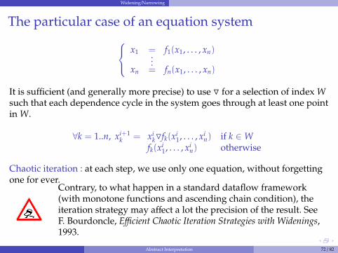
The particular case of an equation system x1 = f1(x1, . . . , xn)...
xn = fn(x1, . . . , xn)
It is sufficient (and generally more precise) to use O for a selection of index Wsuch that each dependence cycle in the system goes through at least one pointin W.
∀k = 1..n, xi+1k = xi
kOfk(xi1, . . . , xi
n) if k ∈Wfk(xi
1, . . . , xin) otherwise
Chaotic iteration : at each step, we use only one equation, without forgettingone for ever.
Contrary, to what happen in a standard dataflow framework(with monotone functions and ascending chain condition), theiteration strategy may affect a lot the precision of the result. SeeF. Bourdoncle, Efficient Chaotic Iteration Strategies with Widenings,1993.
Abstract Interpretation 72 / 82
Polyhedral abstract interpretation
Outline
1 Introduction
2 Intermediate representation : syntax and semantics
3 Collecting semantics
4 Just put some ]...
5 Building a generic abstract interpreter
6 Numeric abstraction by intervals
7 Widening/Narrowing
8 Polyhedral abstract interpretation
9 Readings
Abstract Interpretation 73 / 82
Polyhedral abstract interpretation
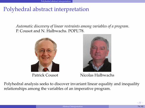
Polyhedral abstract interpretation
Automatic discovery of linear restraints among variables of a program.P. Cousot and N. Halbwachs. POPL’78.
Patrick Cousot Nicolas Halbwachs
Polyhedral analysis seeks to discover invariant linear equality and inequalityrelationships among the variables of an imperative program.
Abstract Interpretation 74 / 82
Polyhedral abstract interpretation
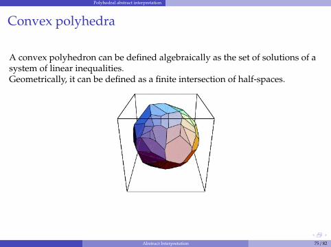
Convex polyhedra
A convex polyhedron can be defined algebraically as the set of solutions of asystem of linear inequalities.Geometrically, it can be defined as a finite intersection of half-spaces.
Abstract Interpretation 75 / 82
Polyhedral abstract interpretation
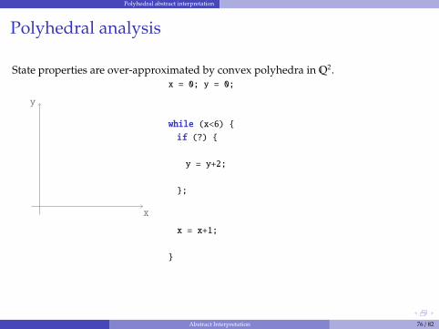
Polyhedral analysis
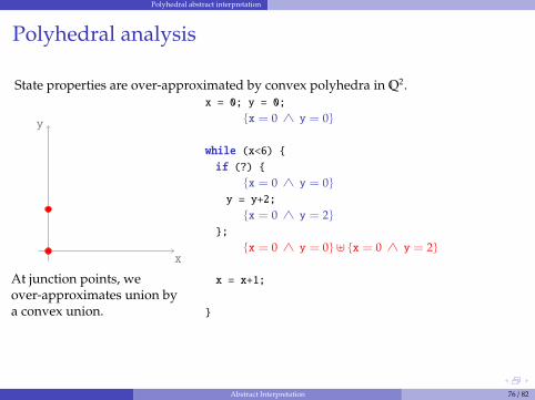
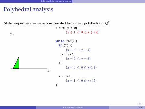
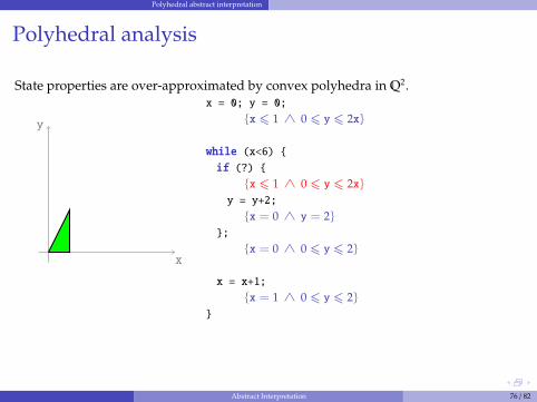
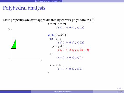
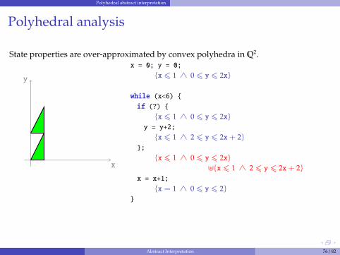
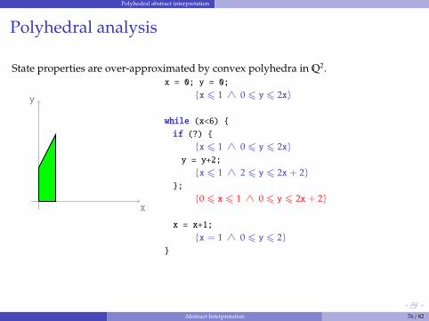
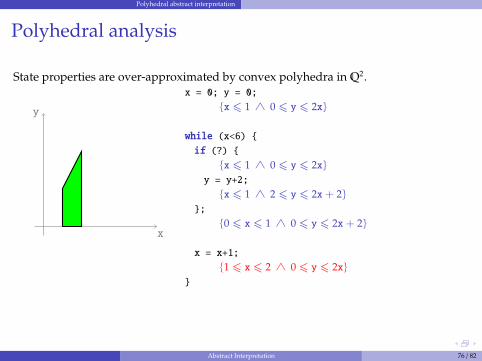
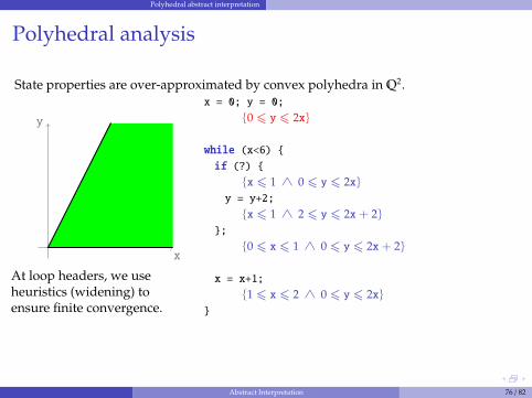
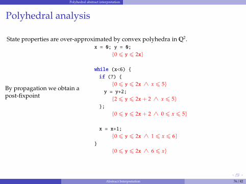
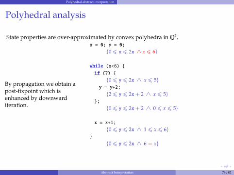
State properties are over-approximated by convex polyhedra in Q2.
x
y
At junction point, we overapproximate union by aconvex union.
x = 0; y = 0;
while (x<6) {
if (?) {
y = y+2;
};
x = x+1;
}
Abstract Interpretation 76 / 82
Polyhedral abstract interpretation
Polyhedral analysis
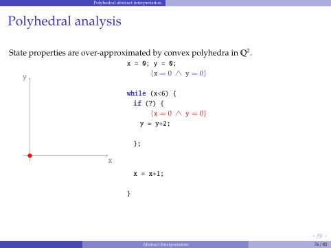
State properties are over-approximated by convex polyhedra in Q2.
x
y
At junction point, we overapproximate union by aconvex union.
x = 0; y = 0;
{x = 0 ∧ y = 0}
while (x<6) {
if (?) {
{x = 0 ∧ y = 0}y = y+2;
};
x = x+1;
}
Abstract Interpretation 76 / 82
Polyhedral abstract interpretation
Polyhedral analysis
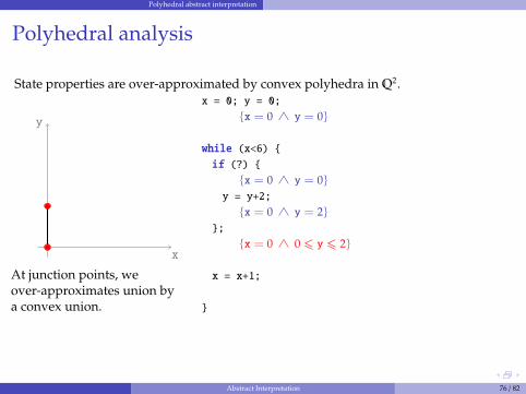
State properties are over-approximated by convex polyhedra in Q2.
x
y
At junction points, weover-approximates union bya convex union.
x = 0; y = 0;
{x = 0 ∧ y = 0}
while (x<6) {
if (?) {
{x = 0 ∧ y = 0}y = y+2;
{x = 0 ∧ y = 2}};
{x = 0 ∧ y = 0}] {x = 0 ∧ y = 2}
x = x+1;
}
Abstract Interpretation 76 / 82
Polyhedral abstract interpretation
Polyhedral analysis
State properties are over-approximated by convex polyhedra in Q2.
x
y
At junction points, weover-approximates union bya convex union.
x = 0; y = 0;
{x = 0 ∧ y = 0}
while (x<6) {
if (?) {
{x = 0 ∧ y = 0}y = y+2;
{x = 0 ∧ y = 2}};
{x = 0 ∧ 0 6 y 6 2}
x = x+1;
}
Abstract Interpretation 76 / 82
Polyhedral abstract interpretation
Polyhedral analysis
State properties are over-approximated by convex polyhedra in Q2.
x
y
At junction point, we overapproximate union by aconvex union.
x = 0; y = 0;
{x = 0 ∧ y = 0}
while (x<6) {
if (?) {
{x = 0 ∧ y = 0}y = y+2;
{x = 0 ∧ y = 2}};
{x = 0 ∧ 0 6 y 6 2}
x = x+1;
{x = 1 ∧ 0 6 y 6 2}}
Abstract Interpretation 76 / 82
Polyhedral abstract interpretation
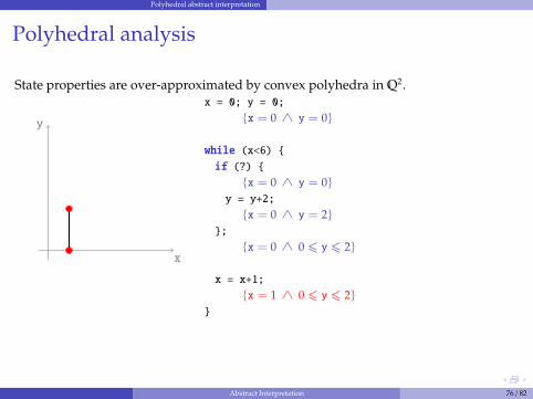
Polyhedral analysis
State properties are over-approximated by convex polyhedra in Q2.
x
y
At junction point, we overapproximate union by aconvex union.
x = 0; y = 0;
{x = 0 ∧ y = 0}] {x = 1 ∧ 0 6 y 6 2}
while (x<6) {
if (?) {
{x = 0 ∧ y = 0}y = y+2;
{x = 0 ∧ y = 2}};
{x = 0 ∧ 0 6 y 6 2}
x = x+1;
{x = 1 ∧ 0 6 y 6 2}}
Abstract Interpretation 76 / 82
Polyhedral abstract interpretation
Polyhedral analysis
State properties are over-approximated by convex polyhedra in Q2.
x
y
At junction point, we overapproximate union by aconvex union.
x = 0; y = 0;
{x 6 1 ∧ 0 6 y 6 2x}
while (x<6) {
if (?) {
{x = 0 ∧ y = 0}y = y+2;
{x = 0 ∧ y = 2}};
{x = 0 ∧ 0 6 y 6 2}
x = x+1;
{x = 1 ∧ 0 6 y 6 2}}
Abstract Interpretation 76 / 82
Polyhedral abstract interpretation
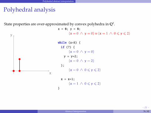
Polyhedral analysis
State properties are over-approximated by convex polyhedra in Q2.
x
y
At junction point, we overapproximate union by aconvex union.
x = 0; y = 0;
{x 6 1 ∧ 0 6 y 6 2x}
while (x<6) {
if (?) {
{x 6 1 ∧ 0 6 y 6 2x}y = y+2;
{x = 0 ∧ y = 2}};
{x = 0 ∧ 0 6 y 6 2}
x = x+1;
{x = 1 ∧ 0 6 y 6 2}}
Abstract Interpretation 76 / 82
Polyhedral abstract interpretation
Polyhedral analysis
State properties are over-approximated by convex polyhedra in Q2.
x
y
At junction point, we overapproximate union by aconvex union.
x = 0; y = 0;
{x 6 1 ∧ 0 6 y 6 2x}
while (x<6) {
if (?) {
{x 6 1 ∧ 0 6 y 6 2x}y = y+2;
{x 6 1 ∧ 2 6 y 6 2x+ 2}};
{x 6 1 ∧ 0 6 y 6 2x}]{x 6 1 ∧ 2 6 y 6 2x+ 2}
x = x+1;
{x = 1 ∧ 0 6 y 6 2}}
Abstract Interpretation 76 / 82
Polyhedral abstract interpretation
Polyhedral analysis
State properties are over-approximated by convex polyhedra in Q2.
x
y
At junction point, we overapproximate union by aconvex union.
x = 0; y = 0;
{x 6 1 ∧ 0 6 y 6 2x}
while (x<6) {
if (?) {
{x 6 1 ∧ 0 6 y 6 2x}y = y+2;
{x 6 1 ∧ 2 6 y 6 2x+ 2}};
{0 6 x 6 1 ∧ 0 6 y 6 2x+ 2}
x = x+1;
{1 6 x 6 2 ∧ 0 6 y 6 2x}}
Abstract Interpretation 76 / 82

Polyhedral abstract interpretation
Polyhedral analysis
State properties are over-approximated by convex polyhedra in Q2.
x
y
At loop headers, we useheuristics (widening) toensure finite convergence.
x = 0; y = 0;
{x 6 1 ∧ 0 6 y 6 2x}O {x 6 2 ∧ 0 6 y 6 2x}
while (x<6) {
if (?) {
{x 6 1 ∧ 0 6 y 6 2x}y = y+2;
{x 6 1 ∧ 2 6 y 6 2x+ 2}};
{0 6 x 6 1 ∧ 0 6 y 6 2x+ 2}
x = x+1;
{1 6 x 6 2 ∧ 0 6 y 6 2x}}
Abstract Interpretation 76 / 82
Polyhedral abstract interpretation
Polyhedral analysis
State properties are over-approximated by convex polyhedra in Q2.
x
y
At loop headers, we useheuristics (widening) toensure finite convergence.
x = 0; y = 0;
{0 6 y 6 2x}
while (x<6) {
if (?) {
{x 6 1 ∧ 0 6 y 6 2x}y = y+2;
{x 6 1 ∧ 2 6 y 6 2x+ 2}};
{0 6 x 6 1 ∧ 0 6 y 6 2x+ 2}
x = x+1;
{1 6 x 6 2 ∧ 0 6 y 6 2x}}
Abstract Interpretation 76 / 82
Polyhedral abstract interpretation
Polyhedral analysis
State properties are over-approximated by convex polyhedra in Q2.
By propagation we obtain apost-fixpoint
which isenhanced by downwarditeration.
x = 0; y = 0;
{0 6 y 6 2x}
while (x<6) {
if (?) {
{0 6 y 6 2x ∧ x 6 5}y = y+2;
{2 6 y 6 2x+ 2 ∧ x 6 5}};
{0 6 y 6 2x+ 2 ∧ 0 6 x 6 5}
x = x+1;
{0 6 y 6 2x ∧ 1 6 x 6 6}}
{0 6 y 6 2x ∧ 6 6 x}
Abstract Interpretation 76 / 82
Polyhedral abstract interpretation
Polyhedral analysis
State properties are over-approximated by convex polyhedra in Q2.
By propagation we obtain apost-fixpoint which isenhanced by downwarditeration.
x = 0; y = 0;
{0 6 y 6 2x ∧ x 6 6}
while (x<6) {
if (?) {
{0 6 y 6 2x ∧ x 6 5}y = y+2;
{2 6 y 6 2x+ 2 ∧ x 6 5}};
{0 6 y 6 2x+ 2 ∧ 0 6 x 6 5}
x = x+1;
{0 6 y 6 2x ∧ 1 6 x 6 6}}
{0 6 y 6 2x ∧ 6 = x}
Abstract Interpretation 76 / 82
Polyhedral abstract interpretation
Polyhedral analysis
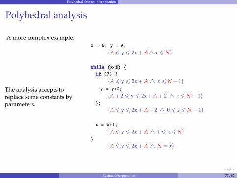
A more complex example.
The analysis accepts toreplace some constants byparameters.
x = 0; y = A;
{A 6 y 6 2x+ A ∧ x 6 N}
while (x<N) {
if (?) {
{A 6 y 6 2x+ A ∧ x 6 N − 1}y = y+2;
{A + 2 6 y 6 2x+ A + 2 ∧ x 6 N − 1}};
{A 6 y 6 2x+ A + 2 ∧ 0 6 x 6 N − 1}
x = x+1;
{A 6 y 6 2x+ A ∧ 1 6 x 6 N}
}
{A 6 y 6 2x+ A ∧ N = x}
Abstract Interpretation 77 / 82
Polyhedral abstract interpretation
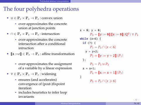
The four polyhedra operationsI ] ∈ Pn × Pn → Pn : convex union
I over-approximates the concreteunion at junction points
I ∩ ∈ Pn × Pn → Pn : intersectionI over-approximates the concrete
intersection after a conditionalintruction
I ~x :=e� ∈ Pn → Pn : affine transformation
I over-approximates the assignmentof a variable by a linear expression
I O ∈ Pn × Pn → Pn : wideningI ensures (and accelerates)
convergence of (post-)fixpointiteration
I includes heuristics to infer loopinvariants
x = 0; y = 0;
P0 = ~y := 0� ~x := 0� (Q2) O P4
while (x<6) {
if (?) {
P1 = P0 ∩ {x < 6}y = y+2;
P2 = ~y := y+ 2� (P1)};
P3 = P1 ] P2
x = x+1;
P4 = ~x := x+ 1� (P3)}
P5 = P0 ∩ {x > 6}
Abstract Interpretation 78 / 82
Polyhedral abstract interpretation
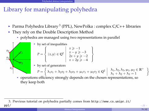
Library for manipulating polyhedra
I Parma Polyhedra Library 3 (PPL), NewPolka : complex C/C++ librariesI They rely on the Double Description Method
I polyhedra are managed using two representations in parallel
s1
s2
s3
r1
r2
I by set of inequalities
P =
(x, y) ∈ Q2
∣∣∣∣∣∣∣∣
x > −1x − y > −32x + y > −2x + 2y > −4
I by set of generators
P =
{λ1s1 + λ2s2 + λ3s3 +µ1r1 +µ2r2 ∈ Q2
∣∣∣∣λ1,λ2,λ3,µ1,µ2 ∈ R+
λ1 + λ2 + λ3 = 1
}I operations efficiency strongly depends on the chosen representations, so
they keep both
3. Previous tutorial on polyhedra partially comes from http://www.cs.unipr.it/ppl/
Abstract Interpretation 79 / 82
Readings
Outline
1 Introduction
2 Intermediate representation : syntax and semantics
3 Collecting semantics
4 Just put some ]...
5 Building a generic abstract interpreter
6 Numeric abstraction by intervals
7 Widening/Narrowing
8 Polyhedral abstract interpretation
9 Readings
Abstract Interpretation 80 / 82
Readings
References (1)
A few articlesI a short formal introduction
P. Cousot and R. Cousot. Basic Concepts of Abstract Interpretation.http://www.di.ens.fr/˜cousot/COUSOTpapers/WCC04.shtml
I technical but very complete (the logic programming part is optional) :P. Cousot and R. Cousot. Abstract Interpretation and Application to Logic Programs.http://www.di.ens.fr/˜cousot/COUSOTpapers/JLP92.shtml
I a nice ap-plication of abstract interpretation theory to verify airbus flight commands
P. Cousot, R. Cousot, J. Feret, L. Mauborgne, A. Mine, D. Monniaux, and X. Rival. TheASTREE Analyser.http://www.di.ens.fr/˜cousot/COUSOTpapers/ESOP05.shtml
Abstract Interpretation 81 / 82
Readings
References (2)
On the web :I informal presentation of AI with nice pictures
http://www.di.ens.fr/˜cousot/AI/IntroAbsInt.html
I a short abstract of various works around AIhttp://www.di.ens.fr/˜cousot/AI/
I very complete lecture noteshttp://web.mit.edu/afs/athena.mit.edu/course/16/16.399/www/
Abstract Interpretation 82 / 82