ABSTRACT

Title of Thesis: BANK FUNDAMENTALS, BANK FAILURES

AND MARKET DISCIPLINE: AN EMPIRICAL ANALYSIS FOR EMERGING MARKETS DURING THE NINETIES

Marco A. Arena Duffoo, Ph. D., 2004 Thesis Directed By: Professor Carmen M. Reinhart, Department of

Economics After the East Asian crisis, there has been a renewed interest in both academic

and policy circles about the role that bank weaknesses play in contributing to

systemic banking crisis. Even though, it has been recognized in the recent theoretical

literature on banking crises that both macroeconomic and bank-level fundamentals

have to be taken into account in the explanation of systemic banking crisis, to

date, there is little cross-country empirical evidence for emerging markets on the

role of bank weaknesses in contributing to both sudden deposit withdrawals and

bank failures. In this context, my thesis analyzes the episodes of systemic

banking crisis in Latin America (Argentina, 1995; Mexico, 1994; and Venezuela,

1994) and East Asia (Indonesia, Korea, Malaysia, Philippines, and Thailand in

1997) using bank-level data in order to answer the following questions. First, to

what extent, did financial conditions of individual banks explain bank failures?

Did only the weakest banks, in terms of their fundamentals, fail in the crisis

countries? Second, did depositors in crisis countries discipline riskier banks by

withdrawing their deposits in such a way that deposit withdrawals could be

considered an act of market discipline? The results for East Asia and Latin America

show that bank-level fundamentals both affect significantly the likelihood of

failure and explain a high proportion of the likelihood of failure of failed banks

(around fifty percent). In East Asian crisis countries, there was little overlap in

the distribution of logit propensity scores between failed and non-failed banks,

implying that mainly the weakest banks failed. However, in Latin American crisis

countries, there was a much clear overlap in the distribution of logit propensity

scores, implying that banking system and macroeconomic shocks are relatively

much more important in Latin America. Regarding market discipline, a stable model

of bank-level fundamentals explains the growth rate of deposits in both regions even

during the peak of the crisis periods. However, in both regions, the relative

contribution of bank level fundamentals during the peak of the crisis periods

declined. In this context, to some degree, the observed deposit withdrawals

represented an informed market response to observable bank weaknesses.

BANK FUNDAMENTALS, BANK FAILURES AND MARKET DISCIPLINE: AN EMPIRICAL ANALYSIS FOR EMERGING MARKETS DURING THE NINETIES

By

Marco A. Arena Duffoo

Thesis submitted to the Faculty of the Graduate School of the University of Maryland, College Park, in partial fulfillment

of the requirements for the degree of Doctor of Philosophy

2004 Advisory Committee: Professor Carmen M. Reinhart, Chair Professor Roger Betancourt Professor John Shea Professor John Wallis Professor I. M. (Mac) Destler

© Copyright by Marco A. Arena Duffoo

2004

ii

Dedication

I dedicate the good things of this work to my mother Ruth Duffoo.

iii

Acknowledgements

I am indebted to Professors Carmen Reinhart, Roger Betancourt, and John Shea for

their advice and guidance. I would like to thank Tamim Bayoumi and Alessandro

Rebucci at the IMF’s Research Department for helpful comments and suggestions of

an earlier version of this work. This work also benefited from valuable comments by

participants at the first meeting of the Latin American Financial Network in Buenos

Aires, Argentina (December, 2003). In particular, I am very graceful to my

discussants Sergio Schmukler (World Bank) and Alicia Garcia-Herrero (Bank of

Spain). Also, I would like to thank Luciana Rios-Benso and Mirian Ramirez at the

Central Bank of Argentina and Venezuela respectively for help me to obtain the data.

Finally, I would like to thank Professor John Wallis for his advice and comments,

Pedro Rodriguez for his support, and in particular to my friend JuanJose Diaz for his

support and help since the beginning of my work.

iv

Table of Contents Dedication ..................................................................................................................... ii Acknowledgements...................................................................................................... iii Table of Contents......................................................................................................... iv List of Tables ............................................................................................................... vi List of Figures ............................................................................................................. vii List of Abbreviations ................................................................................................. viii Chapter 1: Introduction ................................................................................................. 1 Chapter 2: Bank Fundamentals and Bank Failures..................................................... 10

2.1 Review of the Theoretical and Empirical Literature......................................... 10 2.1.1 Review of the Theoretical Literature ......................................................... 10 2.1.2 Review of the Empirical Literature............................................................ 13

2.2 Empirical Methodology .................................................................................... 17 2.2.1 Definition of Failure .................................................................................. 19 2.2.2 Stylized facts: Characteristics of Failed and Non-Failed Financial Institutions........................................................................................................... 21 2.2.3 Probability of Failure: Cross-Sectional Logit estimation .......................... 21 2.2.4 Conditional Probability of Failure: Survival Duration Analysis ............... 22 2.2.5 Calculation of Propensity Scores: Measure of the Relative Contribution of Bank-Level Fundamentals .................................................................................. 24

2.3 Data Sources ..................................................................................................... 24 2.4 Variables ........................................................................................................... 27

2.4.1 Bank-Level Fundamentals ......................................................................... 27 2.4.2 Banking System Variables......................................................................... 31 2.4.3 Macroeconomic Variables ......................................................................... 32

2.5 Empirical Evidence........................................................................................... 33 2.5.1 Characteristics of Failed and Non-Failed Financial Institutions................ 33 2.5.2 Probability of Failure: Cross-Sectional Logit Estimation.......................... 35 2.5.3 Conditional Probability of Failure: Survival Duration Analysis ............... 38 2.5.4 Calculation of Propensity Scores: Measure of the Relative Contribution of Bank-Level Fundamentals .................................................................................. 39

Chapter 3: Bank Fundamentals and Market Discipline .............................................. 43 3.1 Stylized Facts and Review of the Theoretical and Empirical Literature .......... 43

3.1.1 Stylized Facts ............................................................................................. 43 3.1.2 Market Discipline Hypothesis.................................................................... 50 3.1.3 Review of the Empirical Literature............................................................ 51

3.2 Empirical Methodology .................................................................................... 55 3.3 Empirical Evidence........................................................................................... 58

Chapter 4: Conclusions ............................................................................................... 63 Appendices.................................................................................................................. 79

Appendix I: Description of the Logit and Survival Time Model............................ 79 A. Logit Model.................................................................................................... 79 B. Survival Time Model ..................................................................................... 80

v

Appendix II: Description of Data Sample .............................................................. 84 Appendix III: List of Failed Financial Institutions ................................................. 86 Appendix IV: Robustness Check Excluding Mergers and Acquisitions of the Definition of Failure ............................................................................................... 92 Appendix V: Description of the Generalized Methods of Moments (GMM) Estimation ............................................................................................................... 95

References................................................................................................................. 100

vi

List of Tables Table 2.1 Mean Tests for East Asia .................................................................................. 66 Table 2.1 Mean Tests for East Asia (concluded).............................................................. 67 Table 2.2 Mean Tests for Latin America .......................................................................... 68 Table 2.3 Cross-Sectional Logit Estimation for East Asia ............................................... 69 Table 2.4 Cross-Sectional Logit Estimation for Latin America ....................................... 70 Table 2.5 Survival Duration Model for East Asia ............................................................ 71 Table 2.6 Survival Duration Model for Latin America .................................................... 72 Table 2.7 Distributional Analysis of Logit Propensity Scores for Failed and Non-Failed

FIs ............................................................................................................................. 73 Table 3.1 Total Deposit Contraction in Crisis Countries.................................................. 44 Table 3.2 Mean Tests of Deposit Growth Rates in Crisis Countries ................................ 48 Table 3.3 Fixed-Effects Estimation for East Asia (1994-1999) ....................................... 74 Table 3.4 Fixed-Effects Estimation for Latin America (1992-1996) ............................... 75 Table 3.5 Stability of Parameters During the Crisis Period.............................................. 76 Table 3.6 Percentage of Variance Explained by Bank-Level Fundamentals.................... 77 Table 3.7 GMM Estimation (EA: 1994-1999; LA: 1992-1996)....................................... 78 Table IV.1 Mean Tests between Non-Failed FIs and FIs Mergered or Acquired ............ 92 Table IV.2 Cross-Sectional Logit Estimation for East Asia ............................................. 93 Table IV.3 Cross-Sectional Logit Estimation for Latin America ..................................... 94

vii

List of Figures

Figure 2.1 Stock Markets and Total Deposits in Crisis Countries.................................... 46 Figure 2.2 Stock Markets and Total Deposits in Crisis Countries (concluded)................ 47 Figure 2.3 Stock Markets and Total Deposits in Non-Crisis Countries ........................... 49

viii

List of Abbreviations

EA: East Asia.

EMs: Emerging Markets.

FIs: Financial Institutions.

GDP: Gross Domestic Product.

GMM: Generalized Method of Moments.

LA: Latin America.

M&A: Merge and Acquisition

1

Chapter 1: Introduction

In the last two decades, developed and developing countries have experienced significant

episodes of systemic banking crises, which have been more costly in developing areas

than in industrial economies; thus, the prevention of such recurrent episodes has become

a priority of policy1. The most acute among the recent experiences are the financial

problems in some emerging markets (EMs) during the nineties. These episodes have

renewed the interest in academic and policy circles about both the role that individual

financial institutions’ weaknesses play in contributing to bank failures, and the role that

market discipline --the ability of depositors, stockholders, or creditors at large to penalize

banks for bad (poor) performance by withdrawing their deposits or by requiring higher

interest rates-- can play in prudential regulation by encouraging proper risk management

by banks. In this context, my dissertation contributes to this debate by empirically

addressing two main questions: (i) To what extent, did financial conditions of individual

banks explain bank failures? Did only the weakest banks, in terms of their fundamentals,

fail in the crisis countries? (ii) Did depositors in crisis countries discipline riskier banks

by withdrawing their deposits in such a way that deposit withdrawals could be considered

an act of market discipline? 1 See Caprio and Klingebiel (1996, 1999). Regarding the definition of banking crisis, I follow that

given by Sundararajan and Baliño (1991): “… financial crisis is defined as a situation in which a

significant group of financial institutions have liabilities exceeding the market value of their

assets, leading to runs and other portfolio shifts, collapse of some financial firms, and government

intervention”.

2

There are two main reasons to address these questions empirically. First, recent

theoretical research on banking has stressed the role of bank-level fundamentals to

explain both bank failures and depositor discipline. However, there is little cross-country

empirical research at the bank-level that aims to test these hypotheses for EMs. Second,

the answers to these questions are relevant for policy regarding financial regulation and

supervision.

During the last fifteen years, in particular after the East Asian crisis, there has been a

significant increase in the theoretical literature on banking emphasizing that

microeconomic factors related to bank-level fundamentals have to be taken into account

in the explanation of the waves of bank failures and deposit withdrawals that characterize

systemic banking crisis. One stream of this literature argues that the main source of bank

failures rests on bank vulnerabilities due to bad managerial practices reflected in the

deterioration of their portfolio and capital structure prior to the onset of the crisis,2 while

unexpected systemic or macroeconomic shocks just unveil the underlying weakness of

the financial institutions. Another stream in this literature argues that sharp deposit

contractions reflect an act of market discipline, i.e., sudden deposit withdrawals during

the crisis periods represent an informed market response to observable weaknesses in

individual financial institutions (traceable to ex-ante bank characteristics).3

2 Corsetti, Pesenti, and Roubini (1998), Chinn and Kletzer (2000), and Dekle and Kletzer (2001).

3 Jacklin and Battacharya (1988), Chari and Jagannathan (1988), Calomiris et al. (1991),

Calomiris and Gorton (1991), and Jacklin (1993).

3

However, even though there is an extensive theoretical literature on bank failures and

depositor discipline, there is little cross-country empirical evidence using bank-level data

on EMs to test the implications of these hypotheses.4 Most studies that analyze bank

failures and depositors’ discipline at the bank level focus on the experience of the US

commercial banking industry, even though most of the recent episodes of systemic

banking crisis have not occurred in developed countries.5

Understanding the causes or origins of bank failures and sudden deposit contractions has

important policy implications. If bank failures reflect fundamental weaknesses rather than

4 There are some exceptions. The study by Bongini, Claessens and Ferri (2001) investigates the

occurrence of distress and closure decisions in the five East Asian crisis countries (Indonesia,

Korea, Malaysia, Philippines and Thailand) in order to assess the role of bank’s “connections”-

with industrial groups or influential families- in causing and resolving bank failures. Rojas-

Suarez (2001) evaluates an alternative set of indicators based on “markets that work” rather than

just relying on accounting figures in four episodes of systemic banking crisis: East Asia (1997-

1998), Mexico (1994-1995), Venezuela (1994) and Colombia (1982). Martinez-Peria and

Schmukler (2001) evaluate the presence of market discipline for the individual experiences of

Argentina, Chile and Mexico.

5 Whalen (1991), Cole and Gunther (1997), Calomiris (1995, 1997, 1998 and 2000), and

Gonzalez-Hermosillo (1999) develop an empirical analysis of the role of bank fundamentals in

different episodes of banking system problems in the U.S. [Great Depression (1930-1933),

Southwest (1986-1992), Northeast (1991-1992), and California (1992-1993)]. The common

methodology has been the use of multivariate logit analysis and proportional hazard models.

4

depositor confusion in the face of asset value shocks, then policy should strengthen the

financial regulation and supervision system, with emphasis on the set of financial ratios

that reveals conditions conductive to bank failure, forming the basis of an early warning

system. Regarding depositor discipline, if sudden deposit withdrawals are the result of

market discipline actions where depositors assess bank specific risks, then the policy

recommendation is to make banks’ financial information available to depositors both

before and during the run, and to rely more on private market discipline rather than on

full deposit insurance schemes, which reduce depositors’ incentives for bank monitoring

and exacerbate the moral hazard problems reflected in excessive bank risk taking.

However, if sudden deposit withdrawals are unrelated to banks’ portfolio risks then

deposit insurance and other forms of liquidity provision might be considered as useful

instruments to avoid the collapse of the banking system.

The goal of my thesis is to fill the gap between theoretical hypotheses and empirical

testing on bank failures and depositor discipline. I develop the first comparative study at

the micro or bank-level of the recent episodes of systemic banking crisis in East Asia and

Latin America. This allows me to identify and compare underlying patterns not only

across countries but also across regions. My thesis goes beyond and complements

existing empirical macro structural factors present at the origin of crisis.6

6 Kaminsky and Reinhart (1999), Corsetti et al. (1998), Radelet and Sachs (1998), and Demigurc-

Kunt and Detragiache (1997, 1999, 2000). One exception is Honohan (1997), who analyze

systemic banking crisis using aggregate balance sheet indicators.

5

I assemble a comprehensive database of banks gathering, information on balance sheets

and income statements on an annual basis for 14 EMs from the BankScope database and

countries’ Financial Supervisory Agency Reports. As part of the contribution of the

thesis, in the case of Latin America, I assemble a novel database gathering financial

statements directly from Supervisory Financial reports. My dataset include eight

countries from East Asia: Indonesia, Korea, Malaysia, Philippines, Thailand, Singapore,

Hong Kong and Taiwan; and six countries from Latin America: Argentina, Chile,

Colombia, Mexico, Peru and Venezuela. The time span of the data covers the years from

1994 to 1999 for the East Asia sample and from 1992 to 1996 for the Latin America

sample. These samples include the latest episodes of bank runs and failures in both East

Asia and Latin America.

After presenting a review of the existence of the theoretical and empirical literature on

bank failures, Chapter 2 answers the first empirical question; to what extent the waves of

bank failure in the recent episodes of systemic banking crisis in EMs during the nineties

reflected a fundamental deterioration in bank-level conditions. First, I assess if bank-level

heterogeneity is important for explaining cross-country bank failures, i.e., if crisis

countries had weaker banks ex-ante than non-crisis countries rather than just had worse

shocks ex-post. Second, based on the previous results, I evaluate the relative contribution

of bank-level fundamentals in the likelihood of failure, which allow us to determine if

only the weakest banks, in terms of their fundamentals, failed in the crisis countries.

6

In order to perform the first task, given a definition of bank failure, I perform a

descriptive analysis to examine whether failed financial institutions were similar ex-ante

to non-failed financial institutions. Mean tests of bank-level fundamentals are performed,

including market-based indicators such as the rate of decline in bank’s deposits, the

implicit interest rate paid on deposits and loans, and interest rate spreads prior to the

onset of systemic crisis. Then, I estimate the probability of bank failure using a cross-

sectional multivariate logit model for East Asia and Latin America separately, including

crisis and non-crisis countries. Finally, to evaluate the robustness of the cross-sectional

logit results, I relax the assumption that the information used in the logit estimation

accurately reflects unchanging cross-sectional differences in bank condition during the

crisis periods by estimating a survival duration model separately for East Asia and Latin

America for a window of time, using the same set of bank-level fundamentals, and also

aggregate banking and macroeconomic variables, i.e., I include the time dimension in the

estimation.

Regarding the second task, I compute propensity scores, based on the cross-sectional

logit results for individual financial institutions, using only bank-level fundamentals for

failed and non-failed financial institutions to determine their relative contribution to the

likelihood of failure. A distributional analysis of these scores will allow us to evaluate the

degree of overlap between the distribution for failed and non-failed banks in the crisis

countries in order to assess if only the weakest banks failed in the crisis countries.

7

After presenting a review of the existent theoretical and empirical literature on depositor

discipline, and stylized facts surrounding the episodes of sudden deposit withdrawals in

EMs during the last decade, Chapter 3 answers the second empirical question; did

depositors react to bank level fundamentals in such a way that deposit withdrawals could

be considered an action of market discipline in the crisis countries? I conduct panel-data

analysis to test both if riskier banks attract fewer deposits, and if they pay higher interest

rates. The null hypothesis is that deposit withdrawals and deposit interest rates did not

respond to observable weaknesses in individual financial institutions, traceable to ex-ante

bank characteristics, and that deposit runs in the crisis countries were instead episodes of

pure contagion (random withdrawals hypothesis). In addition, I also evaluate the

contribution of bank’s fundamentals relative to banking system and macroeconomic

variables. As a robustness test, I perform GMM estimations to correct for the presence of

potential endogenous effects.

Chapter 4 summarizes the conclusions and policy recommendations. On the whole, my

thesis shows that bank-level fundamentals related to bank asset risk, solvency, liquidity

and profitability explain significantly the probability of bank failure in East Asia and

Latin America. This result support the view that failed banks in the recent systemic crisis

in Emerging Markets during the nineties suffered from fundamental weaknesses in their

asset quality, liquidity, and capital structures. Regarding the relative contribution of bank-

level fundamentals, as opposed to aggregate factors, bank-level fundamentals explain

around fifty percent of the probability of failure of failed banks in the crisis countries in

East Asia and Latin America, which implies that there were many fragile financial

8

institutions with particular ex-ante characteristics that made them more vulnerable to

failure ex-post, i.e., failed banks were predictable weaker ex-ante relative to non-failed

banks.

In the case of East Asian crisis countries, there was little overlapping in the distribution

of propensity scores between failed institutions and non-failed institutions. This result

implies that mainly the weakest institutions failed in the crisis countries, suggesting that

the social costs of the unwarranted closure of solvent institutions (if any) must have been

small. However, in the case of Latin American crisis countries, there was a much clear

overlap in the distribution of aggregate scores between failed institutions and non-failed

institutions, implying that banking system and macroeconomic shocks are relatively more

important in Latin America than in East Asia.

In terms of policy recommendation, my thesis suggests that financial system supervision

should be strengthened, putting emphasis not only on traditional financial ratios

associated with to the CAMEL-rating system, but also on market-based indicators

(deposit interest rates), forming the basis of an early warning system. In addition, given

that macroeconomic and banking system variables affect the probability and timing of

bank failure, financial regulators could rely on stress testing analysis as part of a financial

assessment program in order to assess the vulnerability of a portfolio to major changes in

the macroeconomic environment, making risks more transparent by estimating the

potential losses on a portfolio.

9

Regarding depositor discipline, my thesis shows that a stable model of bank-level

fundamentals explains the growth rate of real deposits in East Asia and Latin America

even during the peak of the crisis periods. This result suggests that depositors attempted

to sort among ex-ante solvent and insolvent banks in the presence of asymmetric

information regarding the effect of shocks to the value of bank assets. However, in both

regions, the relative contribution of bank level fundamentals during the peak of the crisis

periods declined, implying that banking system and macroeconomic shocks played an

important role in the episodes of sudden deposit withdrawals, in particular in Latin

America. In this context, to some degree, the observed deposit withdrawals represented

an informed market response to observable weaknesses in individual financial institutions

In terms of policy recommendation, financial regulators could rely more on elements of

private market discipline (disclosure) as a complement to deposit insurance schemes,

implying that the coverage of such schemes have to be limited in order to maintain or

increase depositors’ incentives for bank monitoring and reduce moral hazard problems

reflected in excessive bank risk taking. Financial institutions should be required to release

general types of public information, including the capital held as a buffer against losses,

risk exposures (credit, market, and operational), risk assessment and management

processes, and the capital adequacy of the institutions, in order to allow market

participants (e.g. depositors) to assess banks’ ability to absorb aggregate shocks and

remain solvent.

10

Chapter 2: Bank Fundamentals and Bank Failures

2.1 Review of the Theoretical and Empirical Literature

2.1.1 Review of the Theoretical Literature

Economic downturns could bankrupt a proportion of borrowers putting banks in distress.

Oviedo (2003) presents a model of business cycles in a small open economy in which

aggregate risk produces sporadic bank failures in a world where banks intermediate

inflows of capital, diversify away idiosyncratic firm risks, issue debt among international

investors, and are subject to capital-adequacy regulation. In this context, economic

downturns trigger a large ratio of poor project returns, reducing the value of the bank’s

portfolios. Under some circumstances, recessions are severe enough that they produce

insolvency of the banking system. On the other hand, aggregate liquidity shocks may

provoke bank failures due to the inability of banks to honor their short-term debts. Chang

and Velasco (1999, 2001) argue that if the banking system’s potential short-term

obligations (demand deposits and foreign short-term debt) exceed its liquidation value,

then a bank run equilibrium exists. In this model, runs may occur only if the banking

system is illiquid; adverse expectations are not, by themselves, sufficient for a run to

occur. In their framework, the more illiquid the banking system, the more vulnerable

(fragile) it will be to exogenous shocks and shifts in expectations.7

7 Potential contagion effects are also considered in this view. Diamond and Rajan (2002) argue

that contagion effects could be caused not only by contractual or asymmetric information links,

11

However, Gavin and Hausmann (1996) argue that aggregate shocks undermine the

viability of financial institutions and create a crisis, but they do not completely explain

banking crises. Bank failures result from the interaction of vulnerability and aggregate

shocks.8 In their argument, “a bank is vulnerable when relatively small shocks to income,

asset quality, or liquidity make the bank either insolvent or illiquid so that its ability to

honor short term debts is brought into doubt” (p. 48).

Why do banks become vulnerable? Alternative hypotheses have been proposed to explain

bank failures putting emphasis on micro-level fundamentals. One major stream of the

literature emphasizes that the main cause of bank failures rests on bad managerial

practices, reflected in the deterioration of banks’ portfolio and capital structures before

the onset of the crisis.

Chinn and Kletzer (2000) and Dekle and Kletzer (2001) present a model of financial

crises in EMs where the source of the financial crisis is found in the interaction between

the microeconomics of private financial intermediation and government macroeconomic

policies. The emphasis on vulnerability of the banking sector bears much in common

but also because bank failures could lead to a contraction in the common pool of liquidity, and

this negative spillover effect raises the likelihood of failure of other banks.

8 In Oviedo’s model, there is not a relative deterioration of banks portfolios and capital structures

before the aggregate productivity shock.

12

with the description and analysis of the East Asian crisis by Corsetti et al. (1998).9 Their

model is based on agency problems in domestic financial intermediation of international

capital flows that originate in an informational advantage for domestic banks in domestic

intermediation, and government provision of guarantees and insurance. Under this

framework, banks intermediate lending to firms, which are subject to idiosyncratic

productivity shocks, implying that firms will become insolvent with positive probability,

in which event banks have the incentives to renegotiate the firm’s debt. Banks not only

accumulate increasingly risky assets, but also become progressively more indebted

through foreign borrowing; under implicit guarantees, this constitutes a contingent

liability for the government. In this context, the crisis evolves endogenously as banks

become increasingly fragile not only because of portfolio deterioration, but also because

of the reduction of the total equity value of the banking sector, in absolute terms and in

proportion to the equity value of the borrowing firms.

On the other hand, as mentioned above, the liquidity crisis hypothesis considers the

degree of bank’s illiquidity as the main source of bank failure. Panics, reflected in runs

by domestic depositors and/or foreign lenders, first articulated by Diamond and Dybvig 9 Corsetti, Pesenti, and Roubini (1998) argue that the East Asian financial crisis was triggered by

fundamental structural and policy distortions. The latter include not only weak macroeconomic

policies, but also weak microeconomic policies, which increased the vulnerability of the banking

sector through the deterioration of banks’ portfolios. In particular, the authors have emphasized

that implicit guarantees led banks to engage in moral hazard lending (the “over-borrowing

syndrome” that was modeled by McKinnon and Pill, 1997).

13

(1983), trigger the crisis, forcing even solvent but illiquid banks to fail because their

liquidation value is lower than its implicit liabilities. Under this hypothesis, liquidity at

the bank level is also a micro-level bank fundamental related to the risk of failure. In this

sense, the liquidity crisis hypothesis involves not only aggregate measures of liquidity in

the system, but also idiosyncratic measures of liquidity at the bank level.

2.1.2 Review of the Empirical Literature

After the East Asian crisis, most of the empirical studies trying to identify the nature and

origins of systemic banking crisis in EMs have focused mainly on macroeconomic factors

and institutional variables.10 At the micro-level, the majority of empirical studies on

banking failures have focus mainly on the U.S. commercial banking industry. Among the 10 See Kaminsky and Reinhart (1999), and Demirguc-Kunt and Detragiache (1997, 1999, and

2000). Some of the explanatory variables used in these studies are the rate of growth of GDP per

capita, the change in terms of trade, the rate of change of the exchange rate, the real interest rate,

the rate of change of the GDP deflator, the ratio of central government budget surplus to GDP,

the ratio of M2 to foreign exchange reserves of the central bank, the ratio of domestic credit to the

private sector to GDP, the ratio of bank liquid reserves to bank assets, the rate of change of the

ratio of bank assets to GDP, a dummy variable for the presence of an explicit deposit insurance

scheme, and an index of the quality of law enforcement. One exception is Honohan (1997) who

performs a systematic evaluation of alternative indicators based on aggregate balance sheet

indicators and indicators of macro-cycles: loan to deposit ratio, foreign borrowing to deposit

ratio, growth rate of credit, share of reserves to deposits, level of lending to the government and

of central bank lending to the banking system.

14

recent contributions in the last decade, Thomson (1991), Whalen (1991), Cole and

Gunther (1995, 1997), and Gonzalez-Hermosillo (1999) develop empirical analyses of

the contribution of bank fundamentals, systemic and macroeconomic factors in different

episodes of banking system problems in the U.S. [Southwest (1986-1992), Northeast

(1991-1992), and California (1992-1993)]. The common methodology used by these

authors has been the use of multivariate logit analysis and proportional hazard models,

and their main findings are that measures of bank solvency and risk, proxied by CAMEL-

rating variables, explain the incidence of bank failures after controlling for aggregate

factors. 11 Calomiris and Mason (2000) provide the first comprehensive econometric

analysis of the causes of bank distress during the Depression. The authors construct a

model of survival duration and investigate the adequacy of bank fundamentals (measures

of bank solvency and risk, related to the CAMEL-rating system) for the period 1930-

1933, after controlling for the effects of county, state, and national-level economic

characteristics. They find that bank fundamentals explain most of the incidence of bank

failure and argue that “contagion” or “liquidity crises” were a relatively unimportant

influence on bank failure risk prior to 1933.12

11 Earlier contributions are Sinkey (1975), Martin (1977), Barth et al. (1985), and Benston (1985).

These studies seek to identify changes in bank-specific variables, related to the CAMEL-rating

analysis, that lead to bank difficulties, and that therefore could be part of an early warning system

of banking problems.

12 Calomiris and Mason (1997) analyze the banking failures during the Chicago panic of June

1932 using the same methodology as in the paper of 2000. The authors conclude that failures

15

However, to date, there is little cross-country empirical evidence that evaluates the

relative contribution of micro-level bank fundamentals in the context of the recent

systemic banking crisis in EMs during the nineties. The main contributors to the literature

of bank failures in EMs are Gonzalez-Hermosillo (1999), Bongini, Claessens and Ferri

(2000), and Rojas-Suarez (2001).

Gonzalez-Hermosillo (1999) analyzes the contribution of bank-level fundamentals and

macroeconomic factors for the Mexican banking crisis in 1994-95. The author finds that

all ex-post measures of risk, and the loan-to assets ratio are associated with the

probability and timing of failure. Bongini, Claessens and Ferri (2001) investigate the

occurrence of bank distress (the financial institution was recapitalized by the government,

received liquidity support, was merged or acquired by other institution, or was intervened

or closed by the government) and closure decisions in five East Asian countries

(Indonesia, Korea, Malaysia, Philippines and Thailand) in order to assess the role of both

bank’s “connections”--with industrial groups or influential families-- and banks’ micro-

weaknesses in causing and resolving bank failures. Among the main findings, CAMEL-

type variables, such as the ratios of loss loan reserves to capital and of net interest income

to total income, help predict subsequent distress; and “connections” increase the

probability of distress and make closure more likely. Rojas-Suarez (2001) evaluates an

alternative set of indicators based on “markets that work” rather than just relying on

accounting figures (CAMEL-type variables) in order to identify in advance impending

during the panic reflected the relative weaknesses of failing banks in the face of a common asset

value shock rather than contagion.

16

banking problems. Using bank-level data for six EMs countries (Korea, Malaysia,

Thailand, Colombia, Mexico and Venezuela) and applying the “signal to noise approach”

methodology, which was used in the study of currency crises by Kaminsky and Reinhart

(1999). The author finds that the capital-to-asset ratio has performed poorly as an

indicator of banking problems in Latin America and East Asia. On the other hand,

interest rates on deposits and spreads have proven to be strong performers.

While extremely informative, the first two of these studies have a number of limitations

as far as the objectives of this paper are concerned. First, case studies are interesting in

their own right. However, one major goal of this paper is to find common ground across

different episodes of systemic banking crises, i.e., to find systematic underlying patterns

that will allow us to make comparisons not only across countries, but also across regions

(Latin America and East Asia) about the relative contribution of micro-level bank

fundamentals in the recent episodes of systemic banking crisis. This information can be

used by policymakers and financial regulators to develop a set of indicators of financial

soundness in order to assess banking systems’ strengths and vulnerabilities.

Second, Bongini et al. (2001)’s analysis of the probability of distress does not include

non-crisis countries in East Asia, which could introduce a bias in the results in the sense

that crisis countries had more bank failures just because they were affected by adverse

aggregate shocks and not because of differences in ex-ante bank fundamentals (crisis

countries had weaker banks ex-ante than non-crisis countries). Also, only a limited

number of bank fundamentals are included in the estimation, not taking into account

17

measures such as the capital-to-assets ratio, the loans-to-assets ratio, measures of

liquidity, and market based indicators such as deposit interest rates, as mentioned by

Rojas-Suarez (2001). This also could introduce a bias, because not all sources of risk

(market, credit and liquidity) have been represented. The definition of distress includes

institutions that were merged or acquired by other financial institutions. However,

mergers and acquisitions could be due to strategic reasons rather than distress. In that

sense, it is necessary to check the robustness of the results to the exclusion of this

category of the definition of distress. A significant fraction of failures occurred in 1998

and 1999. In this sense, one could use financial information for 1997 and 1998 in order to

analyze the financial condition of failed institutions in 1998 and 1999, in addition to the

information as of the end of 1996. In addition, one should include not only bank-level

variables, but also systemic and macroeconomic variables to account for differences

across countries and periods. The authors mention the last two points, arguing that the use

of financial information as of the end 1996 introduces a bias against finding strong

results. Third, neither study calculates the relative contribution of micro-level bank

fundamentals to the probability of bank failure.

2.2 Empirical Methodology

In order to assess whether the waves of bank failure in the recent episodes of systemic

banking crisis in EMs during the nineties reflected a fundamental deterioration in bank-

level conditions, first, I assess if bank-level heterogeneity is important for explaining

cross-country bank failures, i.e., if crisis countries had weaker banks ex-ante than non-

crisis countries rather than just had worse shocks ex-post. Second, based on the previous

18

results, I evaluate the relative contribution of bank-level fundamentals in the likelihood of

failure, which allow us to determine if only the weakest banks, in terms of their

fundamentals, failed in the crisis countries and if cross-sectional differences in bank-level

fundamentals are sufficient or not to explain bank failures.

In order to perform the first task, given a definition of bank failure, I perform a

descriptive analysis to examine in a univariate context whether failed financial

institutions were similar ex-ante to non-failed financial institutions. Mean tests of bank-

level fundamentals are performed, including market-based indicators such as the rate of

decline in bank’s deposits, the implicit interest rate paid on deposits and loans, and

interest rate spreads prior to the onset of systemic crisis. Then, I estimate the probability

of bank failure using a cross-sectional multivariate logit model for East Asia and Latin

America separately, including crisis and non-crisis countries. Finally, to evaluate the

robustness of the cross-sectional logit results, I relax the assumption that the information

used in the logit estimation accurately reflects unchanging cross-sectional differences in

bank condition during the crisis periods by estimating a survival duration model

separately for East Asia and Latin America for a window of time, using the same set of

bank-level fundamentals, and also aggregate banking and macroeconomic variables, i.e.,

I include the time dimension in the estimation.

Regarding the second task, I compute propensity scores, based on the cross-sectional

logit results for individual financial institutions, using only bank-level fundamentals for

failed and non-failed financial institutions to which determine their relative contribution

19

to the likelihood of failure. In addition, a distributional analysis of these scores will allow

us to evaluate the degree of overlapping between the distribution for failed and non-failed

banks in the crisis countries to assess if only the weakest banks failed in the crisis

countries.

2.2.1 Definition of Failure

Most empirical studies of banking failures consider a financial institution to have failed if

it either has received external support or was directly closed. Failure will be identified as

one of the following categories (Bongini, et al., op.cit; and Gonzalez-Hermosillo, 1999):

1. The financial institution was recapitalized by either the Central Bank or an agency

specifically created to tackle the crisis; and/or required a liquidity injection from

the Monetary Authority,

2. The financial institution’s operations were temporally suspended (“frozen”) by

the Government,

3. The Government closed the financial institution,

4. The financial institution was absorbed or acquired by another financial institution.

Under this definition, these categories involve a broader concept of economic failure than

the more restrictive concept of de jure failure (closure). One potential limitation is that

category (4) could include financial institutions that were merged or absorbed for

strategic reasons during the crisis period and not due to insolvency reasons. For this

20

reason, in our statistical tests we will perform a sensitivity analysis excluding this

category.13

In the empirical implementation, a financial institution is considered as failed if it falls in

any of the above categories between 1997 and 1999 in the case of East Asia, between

December 1994 and December 1996 in the case of Argentina and Mexico, and between

January 1994 and December 1995 in the case of Venezuela.14 Thirty one percent of the

sample failed in East Asia and Latin America respectively.

13 This classification was done by looking at Central Banks’ annual reports and daily review of

newspapers, in particular the Asian Wall Street Journal from March 1997 to August 1999. In

addition, I cross my information with two alternative databases assembled by Bongini et al.

(2001) and Laeven (1999).

14 The crisis period is defined since the onset of the crisis (time T): January 1997 (East Asia),

January 1994 (Venezuela), and December 1994 (Argentina and Mexico) up to two more years

(time T+1 and T+2).

21

2.2.2 Stylized facts: Characteristics of Failed and Non-Failed Financial Institutions

First, I examine whether failed institutions were similar ex-ante to non-failed

institutions.15 In this context, mean tests of financial ratios are implemented separately

prior to the onset of the crisis for both regions. Both CAMEL-type variables, which

reflect the market, credit, operational and liquidity risk faced by the financial institutions,

and market-based indicators (deposit interest rates and spreads) are analyzed. This

analysis only reveals if there were statistical differences between failed and non-failed

financial institutions; it does not isolate the contribution of particular variables to the

probability or time of failure.

2.2.3 Probability of Failure: Cross-Sectional Logit estimation

Next, I estimate a cross-sectional multivariate logit model using CAMEL-type variables

(that proxy for bank-level fundamentals), market-based indicators, and country dummies.

The dependent variable takes the value of 1 if the financial institution is identified in any

of the categories of failure during the periods specified in section 2.2.1. I use as

explanatory variables CAMEL-type variables associated with asset quality (the loan loss

provisions to total loans ratio and the total loans to assets ratio), solvency (the total equity

to total assets or liabilities ratio), liquidity (the liquid assets to total liabilities ratio), and

profitability (return on assets). Also, I include the deposit interest rate and spread

15 Given the definition of failure, we classify the financial institutions into failed and non-failed

and conduct the mean and median test over the different financial ratios in the two years prior to

the onset of the crisis.

22

between the loan and deposit interest rate, and the logarithm of total assets to proxy for

the size of the financial institution. See Appendix I, section A, for a detail presentation of

the logit model. CAMEL-type variables and market-based indicators, are measured as of

the end of 1996 for East Asia (Hong Kong, Indonesia, Korea, Malaysia, Philippines,

Singapore, Taiwan, and Thailand), as of the end of 1993 for Venezuela, as of September

1994 for Argentina and Mexico, and as of December 1994 for Chile, Colombia and

Peru.16

2.2.4 Conditional Probability of Failure: Survival Duration Analysis

Under the logit approach discussed above, I estimate the unconditional probability of

failure, under the assumption that bank-level fundamentals (as of the end of 1993,

September 1994, December 1994, and December 1996) accurately reflect unchanging

cross-sectional differences in bank conditions throughout the period January 1997-

December 1999 for East Asia, January 1994-December 1995 for Venezuela, December

1994-December 1996 for Argentina and Mexico. This assumption is not correct, because

the crisis periods in East Asia and Latin America witnessed a continuous deterioration in

asset values, implying that the failure threshold for banks was shifting over that period, 16 Non-crisis countries in East Asia (Hong Kong, Singapore and Taiwan) and Latin America

(Chile, Colombia, and Peru) are included in the estimation to examine the degree of overlap in

bank-level fundamentals between crisis and non-crisis countries. In the case of Latin America, I

performed a robustness check by including only Chile as a non-crisis country, given that

Colombia and Peru were implementing structural reforms at that period of time. No significant

qualitative differences arise. For this reason, I present the results including Colombia and Peru.

23

Declining fundamentals can explain the quality difference between early and late bank

failures during the crisis periods (Calomiris and Mason, 1997).

To evaluate the robustness of the cross-sectional logit results, I estimate a survival

duration model separately for both regions during the periods 1996-1999 for East Asia

and 1993-1996 for Latin America, using the same set of CAMEL-type variables that

proxy for bank level fundamentals, and also I include banking system and

macroeconomic variables, which also could explain early and late bank failures during

the crisis periods according to one stream of the literature on banking crisis reviewed

before.17 The survival duration model allows for changes in the underlying transition

probabilities during the crisis period.

17 Given that I have an exact record of the specific dates of each bank failure, I model each

financial institution’s monthly failure as a function of bank-level fundamentals, banking system

and macroeconomic variables, which are measured annually. I use the same set of CAMEL-type

variables, market-based indicators, and size of the financial institutions as in the cross-sectional

logit estimation. In addition, I include banking system variables, liquidity outside the financial

institution and net foreign liabilities; and macroeconomic variables, the real exchange rate

volatility, GDP growth, and a measure of the stock market. Banking system and macroeconomic

variables are defined in the next section. See Appendix I, section B, for a detailed presentation of

the survival duration model.

24

2.2.5 Calculation of Propensity Scores: Measure of the Relative Contribution of Bank-

Level Fundamentals

Finally, based on the cross-sectional logit results for individual financial institutions, I

compute propensity scores, using only bank-level fundamentals related to asset quality,

solvency, liquidity and profitability for failed and non-failed financial institutions to

determine their relative contribution to the likelihood of failure. In addition, a

distributional analysis of these scores will allow us to evaluate the degree of overlap

between the distribution for failed and non-failed banks in the crisis countries to assess if

only the weakest banks failed in the crisis countries.

2.3 Data Sources

In the case of East Asia,18 financial statements for a sample of 444 financial institutions

have been gathered from BankScope, a comprehensive database of balance sheet and

income statement data for individual financial institutions across the world. This

information covers the period 1995-1999 on annual basis. BankScope collects annual

reports and financial statements from individual financial institutions, which are prepared

according to the various national accounting standards, and adjusts the reported data to

make them comparable across countries as much as possible.

18 Indonesia, Korea, Malaysia, Philippines, and Thailand represent the crisis countries, and Hong

Kong, Singapore, and Taiwan represent the non-crisis countries.

25

The breakdown of data by countries is as follows: (i) 86 commercial banks and 3 other

financial institutions in Indonesia; 19 (ii) 27 commercial banks and 28 other financial

institutions in Korea; (iii) 41 commercial banks and 33 other financial institutions in

Malaysia; (iv) 31 commercial banks and 5 other financial institutions in Philippines; (v)

15 commercial banks and 26 other financial institutions in Thailand; (vi) 43 commercial

banks and 96 other financial institutions in Hong Kong; (vii) 18 commercial banks and 39

other financial institutions in Singapore; (viii) 36 commercial banks and 10 other

financial institutions in Taiwan.

Coverage of the national financial sector in terms of total assets is high for all five

countries and substantial in terms of the number of commercial banks for Malaysia and

Thailand. In terms of total assets, the coverage of the total commercial banking system in

our sample varies between 80% and 100%. The coverage of other financial institutions is

between 47% and 90%. The coverage in terms of number of commercial banks (local and

foreign) is 35% in Indonesia, 34% in Korea, 100% in Malaysia, 63% in Philippines, and

100% in Thailand. In the case of other financial institutions, the coverage is 3% in

Indonesia, 49% in Korea, 55% in Malaysia, 5% in Philippines and 27% in Thailand.

In the case of Latin America, I assemble a novel database by gathering annual balance

sheets and income statements for a sample of 307 banks from official publications of the

19 Other financial institutions include finance companies in the case of Thailand; saving and

investment banks, and merchant banks in the case of Korea and Malaysia; saving banks in the

case Philippines; Islamic and investment banks in the case of Indonesia.

26

national financial supervisor offices of each crisis country (Argentina, Mexico, and

Venezuela), and for non-crisis countries (Chile, Colombia, and Peru) for the period 1992-

1996.20 The coverage of the financial information in terms of total assets is over 80

percent for all the countries due to the fact the banking sector covers a very high share of

the financial system in Latin American countries. As of the end of 1994, the coverage in

terms of total assets is 98 percent in Argentina, over 80 percent in Mexico, and 84 percent

in Venezuela. The breakdown of data by countries is as follows: (i) 171 commercial

banks in Argentina; (ii) 27 commercial banks in Chile; (iii) 21 commercial banks in

Colombia; (iv) 20 commercial banks in Mexico; 21 (v) 21 commercial banks in Peru; and

(vi) 47 commercial banks in Venezuela.22

20 BankScope does not report financial information of banks that failed in Argentina, Mexico and

Venezuela during their respective crisis periods. For this reason, I gathered the information

separately for each crisis country. In this context, the coverage in terms of commercial banks is

basically 100 percent.

21 As of end 1994, there were 32 banks in Mexico. However, 12 banks report information since

1994. For this reason, I only take banks that have al least one year of information previous to

September 1994.

22 See Appendix II for a complete description of the data sample, and Appendix III for the

presentation of the list of failed banks use in the estimations.

27

2.4 Variables

2.4.1 Bank-Level Fundamentals

The theoretical models that stress the role of bank level fundamentals at the root of

banking failures (Kletzer and Chinn and Deckle and Kletzer) establish that as a

consequence of a bad management, the probability of failure is an increasing function of

bank asset risk and solvency (leverage). Chang and Velasco (1999, 2001) stress the role

of bank liquidity. I thus need bank-level variables that proxy for bank asset risk, liquidity,

and solvency.

According to Sinkey (1975), bank financial ratios reflect the variation in bank asset risk

and leverage because they capture the market, credit, operational and liquidity risk faced

by financial institutions. In this sense, bank balance sheets and income statements convey

information about the ex-post consequences of management’s decisions, i.e., they provide

an indirect measure of the managerial performance.

The financial ratios used extensively in the empirical literature for the U.S. commercial

banking industry are those related to the CAMEL-rating system. Regarding asset risk,

ratios of loan loss reserves and loan loss provisions over both total loans and capital are

ex-post measures of asset quality, and the ratio of total loans to total assets represents an

ex-ante measure of asset risk.23 All of these ratios are expected to be positively related to

23 The ratio of non-performing loans over total loans is another traditional measure of asset

quality, but it is not used here because it cannot be found consistently for all the selected

countries, and because this measure varies widely across countries due to different accounting

28

the risk of bank failure. Bank profitability is also considered an ex-ante measure of asset

risk (FDIC, 1997). Sustained levels of profitability allow the financial institution to

increase its capital base and improve its viability, so profitability is negatively related to

the risk of bank failure.24

Solvency is related to the ability to withstand shocks, i.e., how well a financial institution

can absorb losses. However, an operative concept of solvency (positive net worth) is

difficult to measure in practice because of the presence of non-marketable assets or the

absence of liquid markets for some categories of bank assets that make it difficult to

obtain a consistent measure of bank’s asset value. In this context, solvency has been

proxied by the extent of leverage, where the ratio of total capital (total equity plus loss

loan reserves) over total assets is the traditional measure of solvency used in the

empirical literature. 25

standards. On the other hand, ratios of bank’s portfolio concentration, which are related to ex-

ante bank asset risk, are not included due to data availability constraints.

24 However, exceptionally risky projects could be associated with huge rates of return so it is

possible that for some threshold a high degree of profitability could be associated positively with

the risk of failure (Gonzalez-Hermosillo, 1997).

25 In particular, the risk-adjusted capital asset ratio has been the traditional proxy for solvency. In

1988, the Basel Committee on Banking Supervision established a minimum standard of 8 percent

for this ratio.

29

I introduce two additional measures of bank solvency: the ratio of total capital over total

liabilities and over total liabilities plus off-balance sheet items. The measure of the extent

of leverage using liabilities instead of assets provides a more sensible measure of the

bank buffer stock that will serve as a cushion to absorb losses, particularly since the latest

episodes of banking crisis witnessed not only shocks to bank assets, but also to the

deposit base. In addition, the explicit inclusion of off-balance sheet positions produces a

more accurate measure of bank leverage and exposure (Breuer, 2000). Moreover, this

measure accounts for the fact that “the rapid unwinding of positions, as all counter parties

run for liquidity, is characterized by creditors demanding payment, selling collateral, and

putting on hedges, while debtors draw down capital and liquidate other assets. This can

result in extreme market volatility” (IMF, 2002).

Regarding liquidity risk, the traditional indicator of bank liquidity has been the ratio of

liquid assets (cash and reserves, government bonds, and other marketable securities) over

total assets as a measure of the maturity structure of the asset portfolio, which can reflect

excessive maturity mismatches. On the other hand, given that liquid assets allow financial

institutions to meet unexpected deposit withdrawals, the liquidity of assets relative to

liabilities is also a factor affecting the risk of bank failure (Calomiris and Mason, 2000).

For this reason, both ratios, which are negatively related to the risk of bank failure, are

included in the empirical analysis.

In addition, following Rojas-Suarez (2001), I include two additional measures of the

riskiness of individual financial institutions based on market prices rather than accounting

30

figures. I analyze the effect of interest rates (for loans and deposits) and spreads26 on the

probability of bank failure, because such prices are a direct measure of bank default risk

(Calomiris and Mason, op. cit.). An aggressive bidding for deposits could be associated

with a higher likelihood of bank failure, because depositors demand high rates from

banks they perceive as risky, i.e., depositors could have information about bank

vulnerability not captured by CAMEL-type variables, that cause equilibrium deposit rates

to be higher for institutions perceive as risky by depositors.

Even though bank size, measured by total assets, is not considered by the existing

theoretical literature as a bank level fundamental, it is included in the analysis to account

for the fact that larger banks are better able to diversify their loan portfolio, reducing their

asset risk (Calomiris and Mason, op. cit.), and also because “too big to fail” policies

could extend the survival time (reduce the probability of failure) of larger banks.

The use of financial ratios as proxies of fundamental bank attributes provides information

about the symptoms rather than the causes of financial difficulty, in the sense that they

provide leading indicators of incipient crisis (Johnston, et al., 1998). In this sense, I focus

on the near-term fragility (vulnerability) of the financial institutions and not on medium-

to-longer-term vulnerabilities, which requires the identification and evaluation of

potential structural weaknesses that can affect incentives to screen and monitor risks. At

26 The spread equals the difference between the loan interest rate and the implicit deposit interest

rate. The loan interest ate is calculated as the ratio between interest income and total loans. The

deposit interest rate is calculated as the ratio between interest expenses and total deposits.

31

the operational level, this involves a review of the institutional structure, the legal and

regulatory system, corporate governance, the nature of implicit and explicit guarantees,

and the effect of financial reform or liberalization (Johnston, et al. 2000).

2.4.2 Banking System Variables

Banking variables capture potential contagion effects that the banking system (banks and

other financial institutions) as a whole could transmit to individual financial institutions

at the domestic and international level. On the one hand, there is domestic liquidity risk,

where depositor runs from some banks reduce the pool of liquidity over total deposits in

the system and spread negative externalities (spillovers) on other banks under asymmetric

information on the part of the depositors regarding the solvency of the financial

institutions (Diamond and Rajan, 2002). 27 On the other hand, there is international

liquidity risk, where a higher ratio of the financial system’s foreign liabilities over

27 Diamond and Rajan (2002) argue that contagion effects could be caused not only by contractual

or asymmetric information links, but also because bank failures could lead to a contraction in the

common pool of liquidity, and this negative spillover effect raises the likelihood of failure of

other banks. In this context, domestic liquidity risk is proxied by the total amount of liquidity

relative to total deposits outside the bank, i.e., the amount of cash in vaults in the rest of banks in

the system (the summation over the n-1 banks) over the total amount of deposits in the rest of

banks in the system (the summation over the n-1 banks) as a measure of liquidity in the banking

system.

32

international reserves increases its vulnerability to exogenous shocks and shifts in

expectations of international investors (Chang and Velasco, 2001). 28

2.4.3 Macroeconomic Variables

Unexpected macroeconomic shocks undermine the viability of financial institutions

(Hausmann and Gavin, op. cit. and Oviedo, op. cit.). The macroeconomic variables

included in the empirical implementation not only capture the effect of real exchange rate

volatility29, but also the effects of economic activity and stock markets. With respect to

economic activity, I use the annual growth rate of gross domestic product (GDP).

Regarding stock markets, a decline in the total value of bank equities relative to the

overall market value suggests that the aggregate portfolio of the banking system is

deteriorating and becoming increasingly vulnerable in a context of foreign capital

inflows, imperfect prudential regulation, implicit guarantees, and renegotiation of firm

28 International liquidity risk is proxied by the ratio of Bank and Other Financial Institutions’ Net

Foreign Liabilities to Net International Reserves. The data is obtained from the International

Monetary Fund (IMF), International Financial Statistics (IFS). Lines 21, 26c, 41, 41c, and 11c.

29 Real exchange rate volatility is calculated as the monthly average of the standard deviation of

the real effective exchange rate reported by the IMF, IFS. Line rec.

33

debts (Dekle and Kletzer, op. cit.). In this context, a decline in this ratio would be

associated with an increase in the probability of failure (higher financial fragility).30

2.5 Empirical Evidence

2.5.1 Characteristics of Failed and Non-Failed Financial Institutions

Tables 2.1 and 2.2 report mean tests for differences in the bank-level fundamentals

between failed and non-failed financial institutions over two years prior to the onset of

the crisis for East Asia (EA) and Latin America (LA) respectively. In the case of EA,

Table 1 presents the results for the whole sample of financial institutions (FIs) and for

commercial banks only; results are similar for both samples. This table suggests that

failed FIs showed early signs of vulnerability before the onset of the crisis.

Regarding asset risk, failed FIs showed a higher ratio of loss loan reserves and provisions

to total equity, and a higher ratio of loans to total assets, than non-failed FIs, i.e., it is not

only high lending but bad lending that characterizes failed institutions. With respect to

solvency, failed FIs showed a lower ratio of capital to total assets and total liabilities (also

including off-balance sheet items), i.e., higher leverage makes FIs less able to absorb

negative shocks.

30 This ratio is calculated using the stock market index of the banking sector and the general stock

market index. Both variables are averaged over the year using daily information coming from

Bloomberg.

34

Regarding liquidity, failed FIs showed not only a lower ratio of liquid assets to total

assets but also to total liabilities, which made these institutions less able to withstand

unexpected deposit withdrawals. In addition, failed FIs showed lower profitability (return

on assets), which made these institutions less able to increase their capital base and

improve their viability.

With respect to market-based indicators, the results indicate that up to two years before

the onset of the crisis, the implicit deposit interest rate (spread) was higher (lower) for

failed FIs than for non-failed FIs, while there were not statistical differences in the

implicit loan interest rate. The growth rate of real deposits is insignificantly lower for

failed than for non-failed institutions one year before the onset of the crisis. These facts

suggest that failed banks were bidding aggressively to attract deposits, which could also

be consistent with a higher degree of risk taking activities. Regarding spreads, Rojas-

Suarez (op. cit.) argues that narrow spreads should be interpreted differently in emerging

markets than in industrial-country financial markets; in the latter, narrow spreads reflect

efficiency, but in emerging markets they can indicate increased bank risk taking.

In the case of LA, the results in Table 2.2 resemble those for EA regarding asset risk,

solvency, and profitability. Failed banks showed lower liquidity ratios than non-failed

banks only in the period immediately before the onset of the crisis. With respect to

market-based indicators, the results show that in the pre-crisis period the implicit deposit

interest rate was higher for failed banks than for non-failed banks, while there were not

35

statistical differences in the growth rate of deposits.31 This suggests that failed banks had

to offer higher returns in order to obtain financing for high risk taking activities before

the onset of the crisis. In addition, the results show no statistical differences in spreads for

the whole sample32, but a higher implicit interest rate on loans for failed banks than for

non-failed banks in the period prior to the onset of the crisis, suggesting that failed banks

made investments in riskier projects than non-failed banks.

2.5.2 Probability of Failure: Cross-Sectional Logit Estimation

Table 2.3 reports explanatory variables’ marginal effects in the cross-sectional

multivariate logit model for East Asia. According to the results, higher capital relative to

assets or liabilities (also including off-balance-sheet items) is negatively associated with

the probability of failure. A higher level of liquid assets relative to total liabilities and a

higher return on assets reduce the probability of failure. A higher ratio of loans to total

assets has a positive impact on failure. However, the measures of asset quality, loan loss

31 In the case of Venezuela, the rate of deposit growth was lower than the implicit deposit interest

before the onset of the crisis, which implies a transfer problem, i.e., banks were transferring net

resources to the depositors reducing their profitability.

32 In the period previous to the onset of the crisis, spreads in Mexico and Venezuela are lower for

failed banks than for non-failed banks, which are consistent with the results of Rojas-Suarez

(2001), and give support to the hypothesis that lower spreads reflect mainly risk taking activities

in the context of EMs. However, spreads in Argentina are higher for failed banks.

36

reserves and loan loss provisions over total loans, are not significant.33 The latter suggests

that lagging indicators of bank soundness are not good predictors of bank failures under

lax standards for loan classification and loan loss provisioning. In the East Asian crisis

countries, loans were classified as bad loans only if they had been in arrears for six

months or more, and in addition, banks would frequently restructure such loans to reduce

the size of reported portfolio problems (IMF, 1999). The marginal effect of the deposit

interest rate is positive and significant, which implies that banks that bid aggressively for

deposits increase their likelihood of failure. Finally, the logarithm of total assets has the

right sign (negative), but is not significant.

Table 2.4 reports results for LA, which resemble those obtained for EA; bank

fundamentals have the correct sign and explain significantly the probability of failure.

However, the ex-post measure of asset quality (loan loss provisions over total loans) is

marginally significant. As in the case of EA, the marginal effect of the deposit interest

rate is positive and significant. In addition, the size of the bank is negatively associated

with the probability of failure, which would give support the “too big to fail”

hypothesis.34 In this sense, failed financial institutions had particular characteristics in

33 In addition, an estimation using the ratio of loan loss reserves to total loans was performed, and

there were not qualitative differences.

34 This result also could be related to the fact that larger banks are better able to diversify their

loan portfolio, reducing their asset risk (Calomiris and Mason, op. cit).

37

both regions prior to the onset of their respective systemic banking crisis, and bank-level

heterogeneity is important for explaining the variation in failure rates, i.e., banks that

failed during the episodes of bank distress in EMs were observably weaker ex ante (more

vulnerable to negative asset-value shocks) than to banks that survived the crisis.35

Regarding spreads, in the case of EA, the marginal effect of the spread variable is

negative and insignificant. Even though the sign is negative, this result does not support

the hypothesis that lower spreads increase the probability of failure in EMs (Rojas-

Suarez, 2001). For LA, the marginal effect is positive and significant giving, support to

the traditional hypothesis that high spreads increase banks’ fragility.36 As in the case of

deposit interest rate, measures of liquidity, solvency and ex-ante risk (loans-to-assets

ratio) are significant, while the loss loans reserves and loan loss provisions ratios are not

significant.

35 An additional exercise was done for both regions including an ownership dummy (foreign or

domestic). Foreign ownership was negatively associated with the probability of failure.

36 However, this result could be driven by the inclusion of Argentina, because spreads of failed

institutions in Mexico and Venezuela were lower than those of non-failed banks. Only in the case

of Argentina, do we have the usual result obtained in developed economies that failed institutions

had higher spreads than non-failed banks.

38

2.5.3 Conditional Probability of Failure: Survival Duration Analysis

Table 2.5 presents the results of the survival duration model for the period 1996-1999 for

East Asia. After controlling for aggregate banking and macroeconomic variables, the

coefficients of bank-level fundamentals are of predicted sign and significant. Higher

lending relative to assets is positively associated with the timing of failure. Higher

capitalization (relative to assets and liabilities) is negatively associated with the timing of

failure. Higher profitability and higher liquid assets relative to total assets are negatively

associated with the timing of failure. Larger banks are associated with longer survival,

consistent with the “too big to fail” hypothesis. The ex-post measure of asset quality, the

ratio of loan loss provisions to total loans, is marginally significant.

Regarding the aggregate banking and macroeconomic variables, the measure of system

liquidity, which captures potential contagion effects, is positively associated with survival

time in all specifications, i.e., higher liquidity relative to deposits outside the bank gives

positive spillovers, increasing the survival time of the bank. A higher volatility of the real

effective exchange rate index is associated with a lower survival time. As expected,

increases in the economic activity of the sectors in which financial institutions

concentrate their loans are positively associated with the time of survival. The higher the

value of bank stocks relative to the total stock market, the longer the time of survival.

Table 2.6 presents the results for LA. As in the case of EA, after controlling for aggregate

banking and macroeconomic variables, coefficients of bank-level fundamentals related to

asset quality (total loans over total assets), solvency, liquidity and profitability are of

39

predicted sign and significantly explain the time of survival. Results for the banking

system liquidity, the real exchange rate and economic activity are similar to those of EA.

The ex-post measure of asset quality is not significant. Overall, the results show that

measures of (ex-ante) bank asset risk, solvency, liquidity and profitability significantly

affected the survival time of financial institutions in both regions after controlling for the

presence of potential contagion effects in the banking system as a whole, and for shocks

to the macroeconomic environment.37

2.5.4 Calculation of Propensity Scores: Measure of the Relative Contribution of Bank-

Level Fundamentals

I calculate propensity scores for failed and non-failed FIs across crisis and non-crisis

countries based on the individual cross-sectional estimated probabilities of failure, which

allow us to estimate the relative contribution bank-level fundamentals to bank failure for

each group of institutions.38 Table 2.7 shows three main results for EA. First, the average

aggregate degree of vulnerability of non-failed institutions in crisis countries was higher

37 In addition, I performed the survival analysis including spreads. Spreads have a negative sign

but they are not significant in the case of EA. For LA, spreads affect positively the time of failure.

38 The bank-level fundamentals used in the calculations are those related to asset quality (loan

loss provisions ratio, and the total loans to assets ratio), solvency (the ratio of total equity over

total assets or liabilities), liquidity (liquid assets to total liabilities ratio), and profitability (return

on assets).

40

than that of non-failed institutions in non-crisis countries.39 This result suggests that the

differences in the regulatory and supervisory environment in crisis countries could have

given “incentives” to bank managers for high risk taking activities relative to non-crisis

countries.40 Second, the average degree of vulnerability of failed institutions in crisis

countries was higher than that of non-failed institutions in non-crisis countries; only

bank-level fundamentals explain fifty percent of the probability of crisis. This result

implies that there were many fragile FIs with particular ex-ante characteristics that made

them more vulnerable to failure ex-post. Third, in the crisis countries, there is little

overlap in the distribution of aggregate scores between failed institutions and non-failed

institutions. This result implies that mainly the weakest institutions failed in the crisis

countries, suggesting that the social costs of the unwarranted closure of solvent

institutions (if any) must have been small.

39 The average degree of vulnerability for non-failed FIs in crisis countries is even higher if

Philippines is removed from the sample of crisis countries. Philippines was the country least

affected by the crisis in East Asia.

40In addition, mean tests were performed among non-failed FIs between crisis and non-crisis

countries. Non-failed institutions in crisis countries showed lower capitalization, profitability,

liquidity, and spreads; and a higher ratio of loans over total assets than non-distress financial

institutions in non-crisis countries up to two years before the onset of the crisis. This result

suggests that non-failed FIs in crisis countries had a higher degree of vulnerability than non-failed

FIs in non-crisis countries.

41

Table 2.7 also shows the distribution of the propensity scores for LA. As in the case of

EA, the degree of vulnerability of failed institutions in crisis countries was higher than

that of non-failed institutions in non-crisis countries; bank-level fundamentals explain

forty-nine percent of the probability of crisis. However, the aggregate degree of

vulnerability of non-failed institutions in crisis countries was similar to that of non-failed

institutions in non-crisis countries,41 and there is an overlapping in the distribution of

aggregate scores between failed institutions and non-failed institutions in the crisis

countries. These results imply that aggregate factors affecting the banking system are

relatively more important in Latin America than in East Asia, in such a way that a

fraction of healthy institutions may be forced to fail in the context of unexpected

aggregate shocks to the system.42 The latter is consistent with the finding of Kaminsky

41 In the case of LA, non-failed institutions in crisis countries showed similar ratios of

capitalization, profitability, liquidity, but a higher ratio of loans over total assets than non-failed

financial institutions in non-crisis countries prior to the onset of the crisis. This result suggests

that non-failed banks in crisis countries had a similar degree of vulnerability to non-failed banks

in non-crisis countries.

42The previous results are based on a broad definition of failure that includes mergers and

acquisitions (M&A), which could be done for strategic reasons and need not imply a form of

failure. For this reason, I perform a sensitivity analysis excluding from our broad definition of

failure cases in which the financial institution was absorbed or acquired by another financial

institution. The cross-sectional multivariate logit model for both regions showed in tables 3 and 4

is distorted, in particular those results related to asset risk, where a higher ratio of loan loss

provisions to loans is now negatively associated with the probability of failure, in the East Asian

42

and Reinhart (1998) that East Asia and Latin America have different regional patterns for

banking crisis. Systemic banking crises in Latin America have been more volatile and

severe than those in East Asia.

According to these results, bank-level fundamentals are important, but they are not

sufficient to explain cross-countries differences in crisis outcomes because there is some

overlap in the propensity score distributions of financial institutions in non-crisis

countries versus failed institutions in crisis countries, especially for Latin America.

case, and the ratio of total loans to total assets is now not significant (see Appendix IV, Tables

IV.2 and IV.3). In addition, I performed mean tests between Non-Failed Financial Institutions and

Financial Institutions that were Mergered or Acquired (M&A), which show that there were

statistical differences in measures of asset risk, solvency, liquidity, and profitability, suggesting

that M&A banks had higher vulnerability than other non-failed banks (see Appendix IV, Table

IV.1). All together, these results imply that being merged or acquired was part of a bail out policy

rather than a strategic decision during the peak of the crisis period.

43

Chapter 3: Bank Fundamentals and Market Discipline

3.1 Stylized Facts and Review of the Theoretical and Empirical Literature

3.1.1 Stylized Facts

Emerging markets in East Asia and Latin America experienced significant episodes of

sharp deposit contraction during the systemic banking crises that occurred in the nineties.

As we can observe in Table 3.1 and Figure 1, sharp deposit contractions were preceded

by bank asset-value shocks related to abrupt devaluations; sharp increases in interest

rates; and declines in equity and housing prices.43

43 In the case of EA, the first vertical line in the graphs of stock market indexes represents the

official onset of the crisis (the July 2nd devaluation of the bath in Thailand). Subsequent lines

mark the onset of sharp deposit contractions in each country (note that some countries experience

multiple contractions). For LA, the vertical line marks the beginning of the Mexican crisis

(December 1994) and Venezuelan crisis (January 1994). The vertical lines in the graphs of

deposits represent the timing of sudden deposit withdrawals as shown in Table 3.1.

44

Table 3.1 Total Deposit Contraction in Crisis Countries

Author’s calculations based on Central Bank statistical reports, and International Financial Statistics.

Among the crisis countries, Thailand and Korea showed a continuous decline in stock

values in real estate, the banking sector and the general index one year prior to the onset

of the crisis. On the one hand, the stock market decline presumably reduced the quality

and liquidity of banks’ assets and capital base, increasing their vulnerability to aggregate

shocks. On the other hand, the equity decline may also have reduced depositors’

confidence about whether banks would be able to handle the negative impact of the

equity decline, in a context of asymmetric information about bank conditions. In addition,

both countries faced a decline in economic activity prior to the onset of the crisis, putting

more pressure on banks’ asset quality and liquidity due to borrowers’ difficulty repaying

loans. In Indonesia and Malaysia, stock values were driven down by the sharp asset price

declines and devaluations coming from Thailand and Korea, showing a continuous

decline in equity values affecting not only banks’ asset value and capital base, but also

Country Exchange Rate Devaluation (%) Contraction in the Total Deposit BaseThailand Jul. 97: 17.6 Aug. 97 (3.7%)

Jan. 98: 18.8 Feb.98 - Apr. 98 (4.4%)Indonesia Aug. 97 - Oct. 97: 43.6 Nov. 97 (3.7%)

May 98 - Jun. 98: 70.3 Jul. 98 - Aug. 98 (1.8%) Korea Dec. 97: 44.7 Jan. 98 (3%)

Jan. 98 : 14.7 (6.5 % in local currency) Malaysia Dec. 97 - Jan. 98: 29.0 Jan. 98 - May 98 (3.3%)

May 98 - Aug. 98: 12.6 Oct. 98 - Nov. 98 (1.8%) Philippines Dec. 97 - Jan. 98: 22.5 Feb.98 - May. 98 (7.4%)

Feb. 98 (5.0%)Mexico Dec. 94: 14.2 Jan. 95 - Feb. 95 (4.9%)

Jan. 95 : 40.3 Mar. 95 : 17.9 Apr. 95 - Jul. 95 (1.1%)

Argentina Dec. 94 - Feb. 95 (7%)Mar. 95 (9.9%)Apr. 95 - mid May 95 (2.5%)

Venezuela Jan. 92 - Dec. 93 (27.9%) Jun. 93- Dec. 93 (20.3%)

May 94: 17.3 Apr. 94 - Jun 94 (11.5%) Jun 94 : 27.1

45

depositors’ confidence. In this context, deposit runs in Indonesia and Malaysia also

occurred in an environment characterized by sharp declines in asset prices.

In the case of LA, Venezuela showed both a continuous decline in its stock market index

and an increase in real interest rates prior to the onset of the crisis (January 1994). In

addition, there was a decline in the rate of growth of GDP two years prior to the onset of

its crisis. All together, these facts affected directly not only the banking system,

increasing its vulnerability to unexpected aggregate shocks, but also the confidence of

depositors, who began to withdraw their deposits in 1992. Mexico showed a decline in its

stock market in early 1994 due to political instability and an increase in real interest rates

of Government instruments (Cetes and Tesobonos), which were held by banks in

important amounts.44 However, Argentina did not show signs of equity declines or an

increase in interest rates before December 1994. In this sense, the beginning of the crisis

was driven mainly by a contagion effect from the Mexican crisis, due to the risk of

currency devaluation and convertibility.

44 As of December 1994, 50 percent of the commercial banking financial portfolio investment

was in the form of Cetes and Tesobonos.

46

Figure 2.1 Stock Markets and Total Deposits in Crisis Countries STOCK MARKET INDEXES: THAILAND

Constant Local Currency Terms

10210410610810

1010121014101610

12/2

9/95

3/29

/96

6/29

/96

9/29

/96

12/2

9/96

3/29

/97

6/29

/97

9/29

/97

12/2

9/97

3/29

/98

6/29

/98

9/29

/98

BANK REAL ESTATE TOTAL M ARKET

STOCK MARKET INDEXES: KOREAConstant Local Currency Terms

20

120

220

320

420

520

620

720

820

920

1020

12/3

0/95

5/30

/96

10/3

0/96

3/30

/97

8/30

/97

1/30

/98

6/30

/98

11/3

0/98

BANK REAL ESTATE TOTAL MARKET

STOCK MARKET INDEXES: INDONESIAConstant Local Currency Terms

1030507090110130150170190210

12/2

9/95

5/29

/96

10/2

9/96

3/29

/97

8/29

/97

1/29

/98

6/29

/98

11/2

9/98

BANK REAL ESTATE TOTAL MARKET

STOCK MARKET INDEXES: MALAYSIAConstant Local Currency Terms

20

520

1020

1520

2020

2520

3020

12/2

9/95

3/29

/96

6/29

/96

9/29

/96

12/2

9/96

3/29

/97

6/29

/97

9/29

/97

12/2

9/97

3/29

/98

6/29

/98

9/29

/98

1000

3000

5000

7000

9000

11000

13000

REAL STATE TOTAL MARKET BANK

THAILAND : TOTAL DEPOSITS (DEPOSIT MONEY BANKS) In Constant Local Currency Millions

1,900,000

2,000,000

2,100,000

2,200,000

2,300,000

2,400,000

2,500,000

2,600,000

Jan-

96

Mar

-96

May

-96

Jul-9

6

Sep-

96

Nov

-96

Jan-

97

Mar

-97

May

-97

Jul-9

7

Sep-

97

Nov

-97

Jan-

98

Mar

-98

May

-98

Jul-9

8

Sep-

98

KOREA DMB: TOTAL DEPOSITS (DEPOSIT MONEY BANKS)In Constant Local Currency Millions

130,000140,000150,000160,000170,000180,000190,000200,000210,000220,000

Jan-

96

Apr-

96

Jul-9

6

Oct

-96

Jan-

97

Apr-

97

Jul-9

7

Oct

-97

Jan-

98

Apr-

98

Jul-9

8

Oct

-98

INDONESIA: TOTAL DEPOSITS In Constant Local Currency Millions

150,000

160,000

170,000

180,000

190,000

200,000

210,000

220,000Ja

n-96

Mar

-96

May

-96

Jul-9

6

Sep-

96

Nov

-96

Jan-

97

Mar

-97

May

-97

Jul-9

7

Sep-

97

Nov

-97

Jan-

98

Mar

-98

May

-98

Jul-9

8

Sep-

98

Nov

-98

MALAYSIA DMB: TOTAL DEPOSITS (DEPOSIT MONEY BANKS)In Constant Local Currency Millions

160,000

170,000

180,000

190,000

200,000

210,000

220,000

Jan-

96

Apr-

96

Jul-9

6

Oct

-96

Jan-

97

Apr-

97

Jul-9

7

Oct

-97

Jan-

98

Apr-

98

Jul-9

8

Oct

-98

47

Figure 2.2 Stock Markets and Total Deposits in Crisis Countries (concluded)

STOCK MARKET INDEX : ARGENTINAIn Constant Local Currency Terms

10,000

15,000

20,000

25,000

30,000

35,000

Jan-

92

Apr

-92

Jul-9

2

Oct

-92

Jan-

93

Apr

-93

Jul-9

3

Oct

-93

Jan-

94

Apr

-94

Jul-9

4

Oct

-94

Jan-

95

Apr

-95

Jul-9

5

Oct

-95

Jan-

96

Apr

-96

Jul-9

6

Oct

-96

STOCK MARKET INDEX : MEXICOIn Constant Local Currency Terms

1,000

1,500

2,000

2,500

3,000

3,500

4,000

4,500

Jan-

91

Apr

-91

Jul-9

1

Oct

-91

Jan-

92

Apr

-92

Jul-9

2

Oct

-92

Jan-

93

Apr

-93

Jul-9

3

Oct

-93

Jan-

94

Apr

-94

Jul-9

4

Oct

-94

Jan-

95

Apr

-95

Jul-9

5

Oct

-95

STOCK MARKET INDEX : PHILIPPINESIn Constant Local Currency Terms

20

220

420

620

820

1,020

1,220

1,420

1,620

1,820

15-N

ov-

96

15-F

eb-

97

15-M

ay-

97

15-A

ug-

97

15-N

ov-

97

15-F

eb-

98

15-M

ay-

98

15-A

ug-

98

15-N

ov-

98

BANK REAL STATE GENERAL

PHILIPPINES : TOTAL DEPOSITSIn Constant Local Currency Terms

750,000

800,000

850,000

900,000

950,000

1,000,000

1,050,000

1,100,000

1,150,000

Jan-

96

Mar

-96

May

-96

Jul-9

6

Sep-

96

Nov

-96

Jan-

97

Mar

-97

May

-97

Jul-9

7

Sep-

97

Nov

-97

Jan-

98

Mar

-98

May

-98

Jul-9

8

Sep-

98

Nov

-98

In M

illio

ns

MEXICO COMMERCIAL BANKS: TOTAL DEPOSITSIn Constant Local Currency Millions

240,000

290,000

340,000

390,000

440,000

490,000

540,000

590,000

640,000

Feb-

91

May

-91

Aug

-91

Nov

-91

Feb-

92

May

-92

Aug

-92

Nov

-92

Feb-

93

May

-93

Aug

-93

Nov

-93

Feb-

94

May

-94

Aug

-94

Nov

-94

Feb-

95

May

-95

Aug

-95

VENEZUELA COMMERCIAL BANKS: TOTAL DEPOSITSIn Constant Local Currency Terms (Millions)

15,000

16,000

17,000

18,000

19,000

20,000

21,000

22,000

23,000

Jan-

91

Mar

-91

May

-91

Jul-9

1

Sep-

91

Nov

-91

Jan-

92

Mar

-92

May

-92

Jul-9

2

Sep-

92

Nov

-92

Jan-

93

Mar

-93

May

-93

Jul-9

3

Sep-

93

Nov

-93

Jan-

94

Mar

-94

May

-94

Jul-9

4

Sep-

94

Nov

-94

ARGENTINA: TOTAL DEPOSITSIn Constant Local Currency Millions

15,000

20,000

25,000

30,000

35,000

40,000

45,000

50,000

Jan-

92

Apr

-92

Jul-9

2

Oct

-92

Jan-

93

Apr

-93

Jul-9

3

Oct

-93

Jan-

94

Apr

-94

Jul-9

4

Oct

-94

Jan-

95

Apr

-95

Jul-9

5

Oct

-95

VENEZUELA: STOCK MARKET INDEXIn Constant Local Currency Terms

20,000

40,000

60,000

80,000

100,000

120,000

140,000

160,000

Jan-

92

Mar

-92

May

-92

Jul-9

2

Sep

-92

Nov

-92

Jan-

93

Mar

-93

May

-93

Jul-9

3

Sep

-93

Nov

-93

Jan-

94

Mar

-94

May

-94

Jul-9

4

Sep

-94

Nov

-94

Although there was an abrupt decline in the total deposit base in the crisis countries,

which could imply a generalized panic by depositors, the deposit contraction was not the

same for failed and non-failed banks during the peak of the crisis periods. Table 3.2

reports mean tests of the deposit growth rate during the peak of the crisis periods for

failed and non-failed banks:

48

Table 3.2 Mean Tests of Deposit Growth Rates in Crisis Countries

COUNTRY PERIOD NON-FAILED FAILED EA crisis countries 1997-1998 -15.6 -28.2*** Indonesia 1997-1998 -17.5 -36.6*** Korea 1997-1998 -4.7 -18.9* Malaysia 1998 -11.6 -12.4 Thailand 1997-1998 -2.5 -32.4** Argentina 1995 (as of June) -15.3 -28.7*** Mexico 1995 (as of June) -7.9 -16.7** Venezuela 1994 26.3 -8.1*** ***, **, * indicate significant differences between failed and non-failed financial institutions at 1, 5 and 10 percent respectively. Source: Author’s calculations.

Failed banks had a higher rate of deposit decline during the peak of the crisis periods than

non-failed banks, with the exception of Malaysia.45 This asymmetry in depositors’

response to bank asset-value shocks would give preliminary support to the proposition

that depositors sorted among banks during the periods of sudden deposit withdrawals,

i.e., depositors reassessed bank specific risks in such a way that ex ante weaker banks

were considered less prepared to absorb shocks affecting assets value.

45 During the pre-crisis period there were not statistical differences in the growth rate of deposits

between failed and non-failed banks in Latin America and East Asia. However, there were

statistical differences in the deposit interest rate between failed and non-failed banks in both

regions. Failed banks paid higher interest rates to compensate depositors for the higher risk

undertaken. This result is still consistent with the market discipline hypothesis: “Rationing is a

possible but not a necessary result for market discipline. If deposit allocations before the crisis do

not reflect differences between both types of banks it should be the case that the interest rates

paid by failing and merging banks should be higher” (Schumacher, 1996. p.134).

49

In addition, even though Singapore, Taiwan, Colombia, Chile and Peru experienced a

decline in stock values, there were not episodes of sharp deposit contractions in these

countries (see Figure 2). The latter provides us with additional significant information

regarding bank-level heterogeneity to explain cross-country differences in the behavior of

the growth rate of deposits and deposit interest rates.

Figure 2.3 Stock Markets and Total Deposits in Non-Crisis Countries

STOCK MARKET INDEXES: SINGAPOREConstant Local Currency Terms

200

300

400

500

600

700

800

900

12/2

9/95

2/29

/96

4/29

/96

6/29

/96

8/29

/96

10/2

9/96

12/2

9/96

2/28

/97

4/29

/97

6/29

/97

8/29

/97

10/2

9/97

12/2

9/97

2/28

/98

4/29

/98

6/29

/98

BANK REAL STATE GENERAL

STOCK MARKET INDEXES: TAIWANConstant Local Currency Terms

200

400

600

800

1000

1200

1400

1600

1800

2000

12/3

0/95

2/29

/96

4/30

/96

6/30

/96

8/30

/96

10/3

0/96

12/3

0/96

2/28

/97

4/30

/97

6/30

/97

8/30

/97

10/3

0/97

12/3

0/97

2/28

/98

4/30

/98

6/30

/98

4000

5000

6000

7000

8000

9000

10000

BANK REAL ESTATE TOTAL MARKET

TAIWAN:TOTAL DEPOSITSIn Constant Local Currency Terms

10,000

10,500

11,000

11,500

12,000

12,500

13,000

Jan-

96

Mar

-96

May

-96

Jul-9

6

Sep

-96

Nov

-96

Jan-

97

Mar

-97

May

-97

Jul-9

7

Sep

-97

Nov

-97

Jan-

98

Mar

-98

May

-98

Jul-9

8

Sep

-98

Nov

-98

In B

illio

ns (N

.T. D

olla

rs)

SINGAPORE: TOTAL DEPOSITSIn Constant Local Currency Terms

90,000

95,000

100,000

105,000

110,000

115,000

120,000

Jan-

96

Mar

-96

May

-96

Jul-9

6

Sep

-96

Nov

-96

Jan-

97

Mar

-97

May

-97

Jul-9

7

Sep

-97

Nov

-97

Jan-

98

Mar

-98

May

-98

Jul-9

8

Sep

-98

In M

illio

ns

STOCK MARKET INDEX: PERUIn Constant Local Currency Terms

800900

1,0001,1001,2001,3001,4001,5001,6001,700

1/7/

94

3/7/

94

5/7/

94

7/7/

94

9/7/

94

11/7

/94

1/7/

95

3/7/

95

5/7/

95

7/7/

95

9/7/

95

11/7

/95

1/7/

96

3/7/

96

PERU: TOTAL DEPOSITSIn Constant Local Currency Terms

14,00015,00016,00017,00018,00019,00020,00021,00022,00023,00024,000

Jan-

94

Mar

-94

May

-94

Jul-9

4

Sep

-94

Nov

-94

Jan-

95

Mar

-95

May

-95

Jul-9

5

Sep

-95

Nov

-95

Jan-

96

Mar

-96

In M

illio

ns

STOCK MARKET INDEX: CHILEIn Constant Local Currency Terms

800850900950

1,0001,0501,1001,1501,200

1/7/

94

3/7/

94

5/7/

94

7/7/

94

9/7/

94

11/7

/94

1/7/

95

3/7/

95

5/7/

95

7/7/

95

9/7/

95

11/7

/95

1/7/

96

3/7/

96

CHILE: TOTAL DEPOSITSIn Constant Local Currency Terms

7,500

8,000

8,500

9,000

9,500

10,000

Jan-

94

Mar

-94

May

-94

Jul-9

4

Sep

-94

Nov

-94

Jan-

95

Mar

-95

May

-95

Jul-9

5

Sep

-95

Nov

-95

Jan-

96

Mar

-96

In M

illio

ns

50

3.1.2 Market Discipline Hypothesis

Regarding deposit withdrawals, Saunders and Wilson (1994) distinguish among three

situations: “pure” contagion, a mixture of contagion with informed depositors, and a non-

contagious run. In the case of “pure” contagion, depositors are uninformed and unable to

sort between solvent and insolvent banks, so deposit withdrawals occur against both

types of banks.46 In the case of non-contagious withdrawals, depositors reallocate their

deposits from weak banks to healthy banks. Finally, in the case of a mixture, informed

deposits, informed depositors at failing banks withdraw before failure, so the rate of

withdrawals at failing banks are higher than that at non-failing banks.

The last two cases are consistent with the market discipline hypothesis (information

based approach) as developed by Berger (1991), who defines market discipline as a

situation in which economic agents face costs that increase with bank risk and take

actions on the basis of these costs. In a principal-agent problem, the principal (depositor),

by reacting to risk, disciplines the agent (bank manager), reducing in this way ex-ante

excessive risk taking in the banking system, e.g., depositors withdraw their deposits or

require higher interest rates when banks take more risk. [See Jacklin and Battacharya 46This view is related to the liquidity shock approach, as developed in Diamond and Dybvig

(1983), Waldo (1985) and Donaldson (1992), where deposit withdrawals are made without any

consideration of banks’ asset quality and solvency. In this hypothesis, the focus is on bank’s

illiquidity. i.e., solvent but illiquid banks may be forced to fail. However, this approach could be

extended by including heterogeneity in the degree of bank illiquidity in such a way that even a

liquidity shock model would predict that ex-ante weaker banks would be most likely to fail in the

presence of a bank run.

51

(1988), Chari and Jagannathan (1988), Calomiris et al. (1991), Calomiris and Gorton

(1991), and Jacklin (1993)].

As long as there exits heterogeneity across banks in terms of asset quality, liquidity, and

capital structure, depositors could attempt to sort among ex-ante healthy and weak banks

in the context of asymmetric information regarding the effect of aggregate shocks to both

the quality and liquidity of banks’ assets and capital structure. In this sense, deposit runs

could reflect an episode of market discipline, i.e., depositors respond to measures of bank

risk (asset quality, liquidity, and solvency) by withdrawing their deposits and/or by

requiring riskier banks to pay higher interest rates.

3.1.3 Review of the Empirical Literature

The majority of empirical studies on depositors’ discipline focus on the U.S. commercial

banking industry, even though the recent experiences of systemic banking crises have

occurred in emerging markets. Flannery (1998) provides a detailed survey of this

literature. Most of these studies examine market discipline by analyzing either how yields

on uninsured deposits (Baer and Brewer (1986), Hannan and Hanweck (1988), Ellis and

Flannery (1992)) or the level or growth of uninsured deposits (Goldberg and Hudgins

(1996)) respond to measures of bank risk and solvency, as captured by balance sheets,

income statements and market measures of risk.47 The studies of Park (1995) and Park

47 Measures of risk and solvency are related to the CAMEL-rating variables: non-performing

loans as a ratio of total loans, loan loss provisions, the capital to assets ratio, the ratio of real

estate loans to total loans, and return on assets.

52

and Peristiani (1998) analyze market discipline taking into account both yields and

growth of uninsured deposits. The results of these studies support the information-based

approach to bank runs, showing that riskier banks pay higher interest rates, but at the

same time attract fewer uninsured deposits.48

However, the empirical evidence on depositors’ discipline is not very extensive for EMs.

The main contributors to the literature of depositors’ discipline for EM’s are Schumacher

(1996), D’Amato, Grubisic, and Powell (1997), Barajas and Steiner (1999), and

Schmuckler and Martinez-Peria (2001).

Schumacher (1996) examines the 1994-95 Argentine banking panic. Using a bank-level

dataset, the author tests if cross-sectional differences in deposit withdrawals are explained

by measures of bank risk and solvency. As a first step, the author estimates the

probability of bank failures through a multivariate logit approach using accounting

information as of November 1994, finding that the actual capital to required capital ratio,

return on equity, and proxies for liquidity (interbank loans, dollar deposits over total

deposits, and term deposits over total deposits) explain the probability of failure. Then, as

a second step, the author finds that the estimated probability of failure is negatively

48 Cook and Spellman (1994) provide evidence that riskier banks pay higher interest rates even on

insured deposits. In addition, studies of market discipline related to the period of the Great

Depression, (Park (1991), Saunders and Wilson (1996), Calomiris and Mason (1997), and

Calomiris and Mason (2000)) largely support the information-based approach to bank runs.

53

related to the growth rate of deposits, in particular during the peak of the crisis in March

1995. In addition, the author finds that implicit interest rates paid by failing banks

(merged and closed institutions) were higher than those paid by surviving banks.

D’Amato, Grubisic, and Powell (1997) also examine the 1994-95 Argentine banking

panic. The focus of their paper is to use daily deposit data to distinguish the effect of

bank fundamentals from the importance of contagion and generalized macroeconomic

shocks that affect banks simultaneously. Using daily deposit data for a sample of 120

banks, over a four-month period around the panic, the authors estimate a random effects

model of daily changes in deposits as a function of bank fundamentals (as of November

1994) and macroeconomic variables (which vary across time but not across banks). Then,

using a Breusch-Pagan Lagrange Multiplier test the authors indicate that there remain

significant random time effects. As a second step, the authors include lagged deposits of

other banks as a proxy for contagion effects and test again for residual co-movement.

They cannot reject the hypothesis that there is no random time effect, interpreting this

result as evidence of contagion in depositor behavior during the panic.

Barajas and Steiner (2000) study if depositors discipline bank behavior for the period

1986-1999 in Colombia. Using panel-data estimation with semi-annual data, the authors

find that the growth rate of real deposits reacts to bank fundamentals (loss loan

provisions, capital-to- asset ratio, and liquidity), and also to the interest rate paid on

deposits as a measure of return. In addition, the authors analyze the response of banks to

disciplining behavior by depositors, testing directly if bank fundamentals react to changes

54

in deposits, finding that only loss loan provisions behave in a manner consistent with

market discipline.

Schmuckler and Martinez-Peria (2001) evaluate empirically both the interaction between

market discipline and deposit insurance and the impact of banking crises on market

discipline, focusing on the individual experiences of Argentina, Chile and Mexico during

the eighties and nineties. Assembling a bank-level dataset that distinguishes between

insured and uninsured deposits, and using panel data techniques, the authors find that

depositors discipline banks by withdrawing deposits and requiring higher interest rates. In

addition, the authors find that deposit insurance does not appear to diminish the extent of

market discipline and that the depositors’ responsiveness to bank risk is lower during

periods of banking crisis compared to non-panic times.

Most of these empirical studies, with the exception of Martinez-Peria and Schmukler, are

case studies focusing in particular on the Argentine experience. In this sense, while

extremely informative, these studies have a limitation as far as the objectives of this

paper. They do not provide evidence of common underlying patterns in depositors’

discipline across not only countries but also regions, which would give policymakers and

financial regulators more insights regarding the type of information about bank portfolios

and capital structures that should be available to depositors, and for whether regulators

should rely on private market discipline as one of the main components of the regulatory

framework. I will fill this gap by extending the existing empirical evidence not only to

the Mexican and Venezuelan crisis episodes, but also to the East Asian crisis episodes,

55

which have not been studied yet. Also, I include in the sample countries that experience

asset-value shocks, but did not have sudden deposit withdrawals (non-crisis countries) in

order to assess the role of bank-level heterogeneity across country experiences. In this

context, I study to what extent deposit withdrawals constituted an act of market discipline

in the recent episodes of banking problems in Latin America and East Asia.

3.2 Empirical Methodology

In order to assess if depositors react to bank level fundamentals in such a way that deposit

withdrawals could be considered an action of market discipline in the crisis countries, I

test if riskier banks attract fewer deposits. The null hypothesis is that deposit withdrawals

and deposit interest rates did not respond to observable weaknesses in individual financial

institutions, traceable to ex-ante bank characteristics, i.e., that deposit runs in the crisis

countries were episodes of pure contagion (random withdrawals hypothesis). If bank

level fundamentals explain significantly the growth rate of real deposits in the crisis

countries, I interpret this as evidence in favor of the market discipline hypothesis, and

reject the pure contagion hypothesis, which argues that deposit withdrawals are not

related to bank level fundamentals. In order to implement the test, I estimate the

following reduced form equation for the growth rate of real deposits in local constant

currency terms for both regions separately, using the fixed-effect specification:

DEPGRi,j,t = αi + λ t + β’ BANKFUNDi,j,t-1 + γ’ AGG. BANKING j,t +

δ’ MACROj,t + Vi,j,t

Such that i=1,…,N; j=1,…,J; and t=1,…,T

56

DEPGR represents individual bank deposits of bank i at time t in country j. N is the

number of banks in each country. The panel is unbalanced, so T --the number of

observations per bank-- varies across banks. AGG. BANKING represents aggregate

banking variables, which capture potential contagion (spillover) effects of the banking

system on individual institutions, while MACRO is a vector of macroeconomic variables,

which vary across countries and time. BANKFUND is a vector of bank-level

fundamentals. This vector is included with a lag, to account for the fact that balance sheet

information is available to the public with a certain delay. α stands for each bank’s fixed

effect and λ stands for time dummies. Thus, according to the equation, bank deposits are

determined by three main factors: the behavior of deposits in the overall banking system,

the developments in the macro economy, and the evolution of bank-level fundamentals.

In addition, I calculate the contribution of bank-level fundamentals relative to banking

system and macroeconomic variables, using variance decompositions before and during

the crisis period.

In order to evaluate if depositors’ behavior during crisis times responds to bank level

fundamentals as suggested by the market discipline hypothesis, I introduce a dummy

variable for both regions, which takes the value of 1 during the crisis (panic) period:

1997-98 for East Asia and 1994-1995 for Latin America. Then, I interact this dummy

with the bank-specific fundamentals and evaluate if there are statistical differences in the

coefficients between crisis and non-crisis periods. In the case of EA, the crisis dummy

also captures the period where blanket guarantees (full protection for depositors and

creditors) were implemented in Indonesia, Korea, Malaysia and Thailand. In the case of

57

LA, Mexico has an implicit deposit insurance scheme covering the total amount of

deposits; Venezuela has an explicit limited deposit insurance scheme covering up to US$

7,309; and Argentina introduced a limited deposit insurance scheme in April 1995

covering up to US$ 20,000, which was extended up to US$ 30,000 in September 1998. In

this sense, the crisis dummy for LA also evaluates depositors’ discipline in the presence

of deposit insurance schemes. Before the onset of the crisis in East Asia, only Korea,

Singapore and Taiwan had an explicit deposit insurance scheme. In order to capture this

effect, a dummy variable that take the value of one for these countries for the whole

estimation period (since 1996 for Korea) was interacted with bank-level fundamentals.

As a robustness check, I perform generalized method of moments (GMM) estimations

(Arellano-Bover, 1995) to correct for potential endogeneity effects. If bankers are

forward looking, they could anticipate that bank fundamentals at time t-1 affects deposits

at time t . In this sense, banks may try to adjust their risk characteristics to prevent future

deposit withdrawals, which would imply an endogeneity problem (Marinez-Peria and

Schmukler, op.cit.). Also, I will consider as weakly exogenous banking and

macroeconomic variables, even though we could assume that banking system and

macroeconomic variables do not react to individual bank deposits.49 The data sources and

variables are exactly the same as those used in chapter I.

49 See Appendix V for a detail presentation of the GMM estimator, in particular what are the

instruments that will be used in the estimation, and the specification tests used to check if the

assumptions made to calculate the GMM estimators are valid.

58

A second way to approach market discipline is to analyze if depositors discipline bank

risk taking by requiring higher interest rates. However, I will not pursue this approach

due to the lack of adequate data on interest rates paid by each bank on deposits. I can

only generate an implicit interest rate calculated as the share of interest rate expenses

over the total amount of deposits, and not a market interest rate.

3.3 Empirical Evidence

Table 3.3 reports results from estimating the fixed-effects model of deposit growth for

EA. Regarding bank specific fundamentals, FIs with higher ratios of capital, liquidity,

profitability, and lower ratios of loan loss provisions and total loans to total assets, attract

more deposits. 50 In this sense, depositors reassess bank specific risks given asset-value

shocks. The variables that capture potential spillover effects, the measure of banking

liquidity outside the FI and the ratio of net foreign liabilities to total international

reserves, have the right sign and are significant in all specifications, implying that

depositors were sensitive to the total amount of cash in the rest of the financial system

relative to total deposits, and to the ability of the country to repay international investors.

50 Using another measure of ex-post asset quality, the ratio of loan loss reserves to total loans, FIs

with higher ratios of capital, liquidity, profitability, and lower ratios of total loans to total assets,

attracts more deposits. This result provides a robustness test to our previous estimation results. F-

tests indicate that not only bank-level fundamentals, but also aggregate banking and

macroeconomic are jointly significant.

59

Regarding the macroeconomic variables, real exchange volatility has the right sign

(negative) and is highly significant in all specifications. Economic activity has the right

sign (positive) and is also significant in all specifications. F-tests indicate that not only

bank-level fundamentals, but also potential contagion and macroeconomic variables, are

jointly significant.51

In addition, I analyze depositors’ discipline during the peak of the crisis period (1997-

1998) in order to assess whether bank fundamentals explain deposit changes at a time

when all crisis countries implemented blanket guarantees in order to prevent bank runs.

Table 3.5 reports the interaction terms between bank fundamentals and a crisis dummy

that takes the value of 1 in the period 1997-1998. According to the results, there are

changes in the coefficients related to the ratios of total loans and liquidity to total assets.

These coefficients have a higher absolute value during crisis years, implying that

depositors care more about bank exposure in the loan market and the bank’s ability to

repay deposits. There is no change in the coefficients related to solvency and

profitability, implying that depositors show a stable behavior regarding these 51 In order to capture the effect of the explicit deposit insurance scheme in Korea, Singapore and

Taiwan, a dummy variable that took the value of one for these countries for the whole estimation

period (since 1996 for Korea) was interacted with bank-level fundamentals. There were not

significant differences in the coefficients of the loan to asset ratio, solvency, liquidity, and

profitability measures. However, the loan loss provisions ratio was not significant for the

countries with deposit insurance. This result would suggest that the presence of an explicit

deposit insurance scheme did not preclude a risk assessment by part of the depositors.

60

fundamentals. However, the coefficient on the loan loss provisions ratio is only

marginally significant during the crisis period, which suggests that lagging variables

related to bank asset quality do not convey relevant information to depositors during the

peak of the crisis period. This may be a consequence of lax accounting practices in EA

regarding loan loss provisioning and classification.

The contribution of bank-level fundamentals relative to banking system and

macroeconomic variables is shown in Table 3.6.52 The percentage of the variance

generally explained by fundamentals is around 35 percent over the whole estimation

period. However, during the peak of the crisis, the percentage of the variance explained

by fundamentals drops to around 21 percent, reflecting the importance of aggregate

shocks in the crisis period.

Table 3.4 reports results from estimating the fixed-effects model for deposit growth for

LA. Regarding bank specific fundamentals, FIs with higher ratios of capital and liquidity,

and lower ratios of loss loan provisions and total loans to total assets, attract more

deposits. As in the case of EA, depositors reassess bank specific risks given asset-value

shocks. In addition, the variables that capture potential spillover effects have the right

sign and are significant in all specifications. Real exchange volatility has the right sign

52 In order to calculate the percentage of the adjusted R-squared explained by specific

fundamentals, once the fixed effects and time dummies have been removed, I run a regression

with macroeconomic and potential contagion variables, then I add specific fundamentals and

compute the percentage increase in the adjusted R-squared.

61

(negative) and is highly significant in all specifications. Economic activity has the right

sign (positive) and is significant in all specifications. F-tests indicate that not only bank-

level fundamentals, but also potential contagion and macroeconomic variables, are jointly

significant.

Table 3.5 reports the interaction terms between bank fundamentals and a crisis dummy

that takes the value of 1 in 1994 for Venezuela and 1995 for Argentina and Mexico.

According to the results, there are changes in the coefficients related to solvency,

liquidity, and the ratio of total loans over total assets, which continue to be significant,

with the exception of solvency, with a higher absolute value in the case of the ratio of

total loans and liquidity, implying that depositors care about bank exposure in the loan

market and about the bank’s ability to repay deposits during the crisis. There is no change

in the coefficients related to asset quality and profitability, implying that depositors show

a stable behavior regarding these fundamentals.

The contribution of bank-level fundamentals to the variance of deposit growth is shown

in Table 3.6. The percentage of variance explained by fundamentals is between 31 and 42

percent over the whole estimation period, depending on specification. However, the

percentage of the variance explained by fundamentals averages 22 percent during the

peak of the crisis, reflecting an increase in the relative importance of aggregate shocks in

the crisis period, as in the case of EA. Table 3.7 reports the results of the GMM

62

estimation for both regions. Bank-level fundamentals individually and jointly explain the

growth rate of real deposits after correcting for potential endogenous effects.53

53 In the case of East Asia, the coefficients of the loan loss provisions and return on assets

variables are not significant, and in the case of Latin America, the return on assets is not

significant. This could be related to the reduction of sample size, given that lags of the variables

are used in order to generate the instruments in the estimation. However, the reduction in the

number of observations, the results obtained in the fixed-effect estimation proved to be robust

after correcting for potential endogenous effects.

63

Chapter 4: Conclusions

Bank-level fundamentals related to ex-ante bank asset risk, solvency, liquidity and

profitability affected significantly the probability and time of bank failure in East Asia

and Latin America. This result support the view that failed banks in the recent systemic

crisis in Emerging Markets during the nineties suffered from fundamental weaknesses in

their asset quality, liquidity, and capital structures prior to the onset of the crisis. In

addition, macroeconomic and banking system variables explain the likelihood of failure,

implying that aggregate shocks mainly unveiled prior bank weaknesses during the crisis

episodes.

Regarding the relative contribution of bank-level fundamentals, as opposed to systemic

and macroeconomic factors, bank-level fundamentals explain around fifty percent of the

probability of bank failure in East Asia and Latin America, which implies that there were

many fragile financial institutions with particular ex-ante characteristics that made them

more vulnerable to failure ex-post. In the case of East Asian crisis countries, there was

little overlapping in the distribution of aggregate scores between failed institutions and

non-failed institutions. This result implies that mainly the weakest institutions failed in

the crisis countries, suggesting that the social costs of the unwarranted closure of solvent

institutions (if any) must have been small. However, in the case of Latin American crisis

countries, there was some overlapping in the distribution of aggregate scores between

failed institutions and non-failed institutions in the crisis countries. These results imply

that aggregate factors, affecting the banking system, are relatively more important in

Latin America than in East Asia, in such a way that a fraction of healthy institutions may

64

be forced to fail in the context of unexpected aggregate shocks to the system. The latter is

consistent with the finding of Kaminsky and Reinhart (1998) that East Asia and Latin

America have different regional patterns for banking crisis. Systemic banking crisis in

Latin America had been more volatile and severe than those in East Asia.

In terms of policy recommendation, the results suggest that financial system supervision

should be strengthened, putting emphasis on not only traditional financial ratios

associated to the CAMEL-rating system, but also market-based indicators (deposit

interest rates), forming the basis of an early warning system. In addition, given that

macroeconomic and banking system variables affect the probability and time of bank

failure, financial regulators could rely on stress testing analysis as part of an financial

assessment program in order to assess the vulnerability of a portfolio to major changes in

the macroeconomic environment, making risks more transparent by estimating the

potential losses on a portfolio.

In East Asia and Latin America, a stable model of bank-level fundamentals explains the

growth rate of real deposits even during the peak of the crisis periods. In this sense, this

would suggest that depositors attempted to sort among ex-ante solvent and ex-ante

insolvent banks in the presence of asymmetric information regarding the effect of shocks

to the value of bank assets. However, in both regions, the relative contribution of bank

level fundamentals during the peak of the crisis periods declined, implying that aggregate

shocks played an important role in the episodes of sudden deposit withdrawals. In this

65

context, to some degree, the observed deposits withdrawals represented an informed

market response to observable weaknesses in individual financial institutions.

In terms of policy recommendation, these results open the door to the discussion at the

policymaker level of the relevance of financial information disclosure by financial

regulators in order to build up a more effective market discipline as a component of the

regulatory framework. Financial regulators could rely more on elements of private market

discipline (disclosure) as a complement of deposit insurance schemes, implying that the

coverage of that schemes have to be limited in order to reduce depositors’ incentives for

bank monitoring besides the moral hazard problems reflected in excessive bank risk

taking. Financial institutions should release general types of public disclosure, including

the capital held as a buffer against losses, risk exposures (credit, market, and operational

risks), risk assessment and management processes, and the capital adequacy of the

institutions, in order to allow market participants (e.g. depositors) to assess the bank

ability to absorb aggregate shocks and remain solvent.

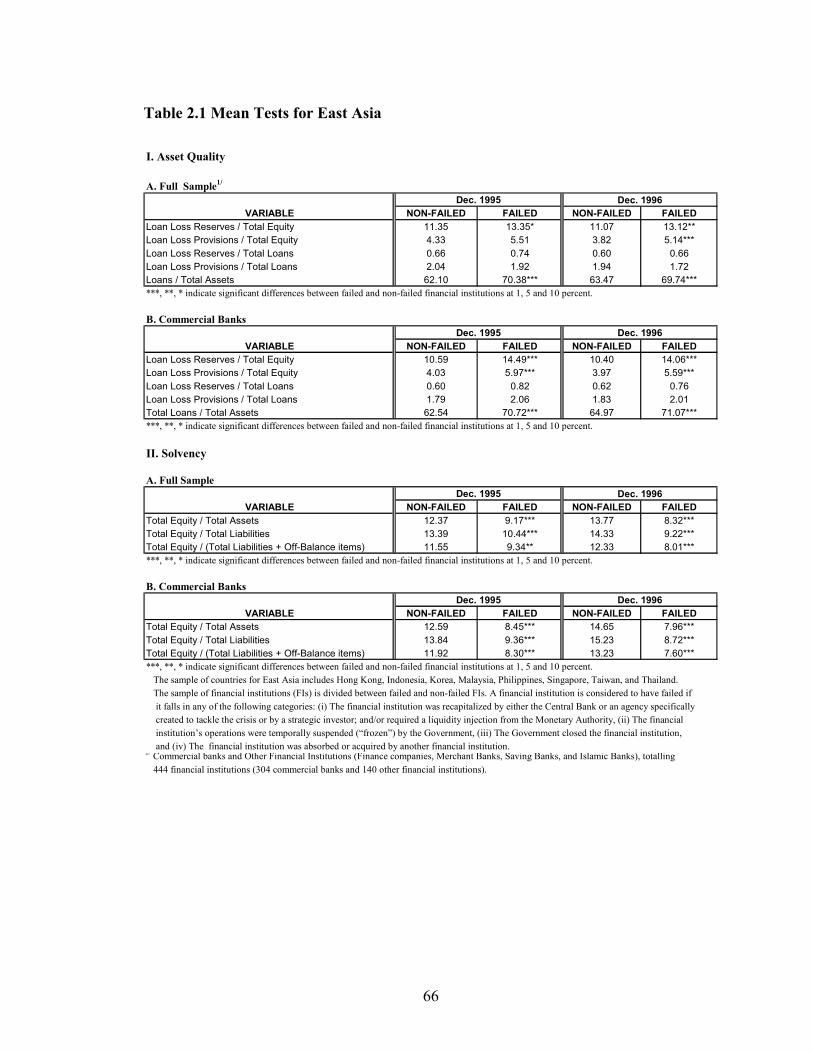
66

Table 2.1 Mean Tests for East Asia I. Asset Quality

A. Full Sample1/

Dec. 1995VARIABLE NON-FAILED FAILED NON-FAILED FAILED

Loan Loss Reserves / Total Equity 11.35 13.35* 11.07 13.12**Loan Loss Provisions / Total Equity 4.33 5.51 3.82 5.14***Loan Loss Reserves / Total Loans 0.66 0.74 0.60 0.66Loan Loss Provisions / Total Loans 2.04 1.92 1.94 1.72Loans / Total Assets 62.10 70.38*** 63.47 69.74******, **, * indicate significant differences between failed and non-failed financial institutions at 1, 5 and 10 percent.

B. Commercial BanksDec. 1995

VARIABLE NON-FAILED FAILED NON-FAILED FAILEDLoan Loss Reserves / Total Equity 10.59 14.49*** 10.40 14.06***Loan Loss Provisions / Total Equity 4.03 5.97*** 3.97 5.59***Loan Loss Reserves / Total Loans 0.60 0.82 0.62 0.76Loan Loss Provisions / Total Loans 1.79 2.06 1.83 2.01Total Loans / Total Assets 62.54 70.72*** 64.97 71.07******, **, * indicate significant differences between failed and non-failed financial institutions at 1, 5 and 10 percent.

II. Solvency

A. Full SampleDec. 1995

VARIABLE NON-FAILED FAILED NON-FAILED FAILEDTotal Equity / Total Assets 12.37 9.17*** 13.77 8.32***Total Equity / Total Liabilities 13.39 10.44*** 14.33 9.22***Total Equity / (Total Liabilities + Off-Balance items) 11.55 9.34** 12.33 8.01******, **, * indicate significant differences between failed and non-failed financial institutions at 1, 5 and 10 percent.

B. Commercial BanksDec. 1995

VARIABLE NON-FAILED FAILED NON-FAILED FAILEDTotal Equity / Total Assets 12.59 8.45*** 14.65 7.96***Total Equity / Total Liabilities 13.84 9.36*** 15.23 8.72***Total Equity / (Total Liabilities + Off-Balance items) 11.92 8.30*** 13.23 7.60******, **, * indicate significant differences between failed and non-failed financial institutions at 1, 5 and 10 percent. The sample of countries for East Asia includes Hong Kong, Indonesia, Korea, Malaysia, Philippines, Singapore, Taiwan, and Thailand. The sample of financial institutions (FIs) is divided between failed and non-failed FIs. A financial institution is considered to have failed if it falls in any of the following categories: (i) The financial institution was recapitalized by either the Central Bank or an agency specifically created to tackle the crisis or by a strategic investor; and/or required a liquidity injection from the Monetary Authority, (ii) The financial institution’s operations were temporally suspended (“frozen”) by the Government, (iii) The Government closed the financial institution, and (iv) The financial institution was absorbed or acquired by another financial institution.2/ Commercial banks and Other Financial Institutions (Finance companies, Merchant Banks, Saving Banks, and Islamic Banks), totalling 444 financial institutions (304 commercial banks and 140 other financial institutions).

Dec. 1996

Dec. 1996

Dec. 1996

Dec. 1996

67

Table 2.2 Mean Tests for East Asia (concluded) III. Liquidity

A. Full Sample1/

Dec. 1995VARIABLE NON-FAILED FAILED NON-FAILED FAILED

Liquid Assets / Total Assets 23.31 16.93*** 22.23 17.46***Liquid Assets / Total Liabilities 26.98 18.70*** 24.43 19.01***Due to Banks / Total Deposits 24.29 29.59 18.77 29.06******, **, * indicate significant differences between failed and non-failed financial institutions at 1, 5 and 10 percent.

B. Commercial BanksDec. 1995

VARIABLE NON-FAILED FAILED NON-FAILED FAILEDLiquid Assets / Total Assets 23.58 18.08*** 23.13 18.74***Liquid Assets / Total Liabilities 26.89 19.78*** 25.25 20.34***Due to Banks / Total Deposits 22.78 26.42 17.74 26.99*****, **, * indicate significant differences between failed and non-failed financial institutions at 1, 5 and 10 percent.

IV. Earnings and Profitability

A. Full SampleDec. 1995

VARIABLE NON-FAILED FAILED NON-FAILED FAILEDNet Interest Margin 4.06 3.44*** 4.11 3.38***Return on Assets 1.62 1.07*** 1.60 1.01******, **, * indicate significant differences between failed and non-failed financial institutions at 1, 5 and 10 percent.

B. Commercial BanksDec. 1995

VARIABLE NON-FAILED FAILED NON-FAILED FAILEDNet Interest Margin 4.52 3.87*** 4.47 3.68***Return on Assets 1.62 1.06*** 1.68 1.07******, **, * indicate significant differences between failed and non-failed financial institutions at 1, 5 and 10 percent.

V. Interest Rates and Deposits

A. Full SampleDec. 1995

VARIABLE NON-FAILED FAILED NON-FAILED FAILEDGrowth Rate of Deposits 19.34 18.05 18.24 17.48Loans Interest Rate 14.73 15.01 14.81 15.57Deposit Interest Rate 9.05 11.16*** 9.19 11.67***Spread 7.19 4.96*** 6.93 5.64******, **, * indicate significant differences between failed and non-failed financial institutions at 1, 5 and 10 percent.

B. Commercial BanksDec. 1995

VARIABLE NON-FAILED FAILED NON-FAILED FAILEDGrowth Rate of Deposits 20.31 18.38 18.24 17.75Loans Interest Rate 14.88 15.29 14.89 15.69Deposit Interest Rate 8.67 11.18*** 8.96 11.80***Spread 7.19 4.94*** 6.99 4.99******, **, * indicate significant differences between failed and non-failed financial institutions at 1, 5 and 10 percent. The sample of countries for East Asia includes Hong Kong, Indonesia, Korea, Malaysia, Philippines, Singapore, Taiwan, and Thailand. The sample of financial institutions (FIs) is divided between failed and non-failed FIs. A financial institution is considered to have failed if it falls in any of the following categories: (i) The financial institution was recapitalized by either the Central Bank or an agency specifically created to tackle the crisis or by a strategic investor; and/or required a liquidity injection from the Monetary Authority, (ii) The financial institution’s operations were temporally suspended (“frozen”) by the Government, (iii) The Government closed the financial institution, and (iv) The financial institution was absorbed or acquired by another financial institution.2/ Commercial banks and Other Financial Institutions (Finance companies, Merchant Banks, Saving Banks, and Islamic Banks), totalling 444 financial institutions (304 commercial banks and 140 other financial institutions).

Dec. 1996

Dec. 1996

Dec. 1996

Dec. 1996

Dec. 1996

Dec. 1996

68

Table 2.3 Mean Tests for Latin America

Commercial Banks 1/2/ 3/

I. Asset QualityT-2 T-1

VARIABLE NON-FAILED FAILED NON-FAILED FAILEDLoan Loss Provisions / Total Equity 8.58 8.61 7.32 9.69*Loan Loss Provisions / Total Loans 2.05 1.35 1.92 1.70Loans / Total Assets 47.21 54.14*** 48.62 55.46******, **, * indicate significant differences between failed and non-failed financial institutions at 1, 5 and 10 percent.

II. SolvencyT-2 T-1

VARIABLE NON-FAILED FAILED NON-FAILED FAILEDTotal Equity / Total Assets 14.65 13.49 14.86 12.56**Total Equity / Total Liabilities 17.18 16.52 18.89 15.16*****, **, * indicate significant differences between failed and non-failed financial institutions at 1, 5 and 10 percent.

III. LiquidityT-2 T-1

VARIABLE NON-FAILED FAILED NON-FAILED FAILEDLiquid Assets / Total Assets 23.99 22.29 24.13 20.33**Liquid Assets / Total Liabilities 27.78 25.82 26.38 23.26****, **, * indicate significant differences between failed and non-failed financial institutions at 1, 5 and 10 percent.

IV. ProfitabilityT-2 T-1

VARIABLE NON-FAILED FAILED NON-FAILED FAILEDReturn on Assets 1.31 1.01 1.07 0.14******, **, * indicate significant differences between failed and non-failed financial institutions at 1, 5 and 10 percent.

V. Interest Rates and DepositsT-2 T-1

VARIABLE NON-FAILED FAILED NON-FAILED FAILEDGrowth Rate of Deposits 18.01 19.94 15.02 14.01Loans Interest Rate 18.32 23.89*** 18.99 21.44**Deposit Interest Rate 9.92 12.02** 10.51 13.03**Spread 11.19 14.43*** 11.42 13.97*****, **, * indicate significant differences between failed and non-failed financial institutions at 1, 5 and 10 percent.1/ The sample of countries for Latin America includes Argentina, Chile, Colombia, Mexico, Peru, and Venezuela.2/ The sample of financial institutions for Latin America only includes commercial banks because they cover a very high proportion (over80 percent) of the financial system in terms of assets. There are 307 commercial banks in the sample.The sample of commercial banks is divided between failed and non-failed banks. A commercial bank is considered to have failed ifit falls in any of the following categories: (i) The commercial bank was recapitalized by either the Central Bank or an agency specifically created to tackle the crisis or by a strategic investor; and/or required a liquidity injection from the Monetary Authority, (ii) The commercial bank's operations were temporally suspended (“frozen”) by the Government, (iii) The Government closed the commercial bank,and (iv) The commercial bank was absorbed or acquired by another financial institution.3/ T-1 represents Dec. 93 for Venezuela, Sep. 94 for Argentina and Mexico, Dec, 94 for Chile, Colombia, and Peru. T-2 representsDec. 92 for Venezuela, and Dec. 93 for Argentina, Chile, Colombia, Mexico, and Peru.

69

Table 2.4 Cross-Sectional Logit Estimation for East Asia (Marginal Effects) 1/ 2/

(1) (2) (3) (4) (5) (6)

Loan Loss Provisions / Total Loans -0.014 -0.014 -0.046 -0.008 -0.009 -0.0280.860 0.868 0.635 0.884 0.883 0.619

Total Loans / Total Assets 0.012 ** 0.012 ** 0.010 ** 0.014 ** 0.014 ** 0.014 **0.023 0.022 0.043 0.009 0.008 0.007

Total Equity / Total Assets -0.030 ** -0.028 *0.052 0.087

Total Equity / Total Liabilities -0.022 * -0.0200.073 0.139

Total Equity / (Total Liab. + OBS.) -0.002 * -0.0010.090 0.922

Liquid Assets / Total Liabilities -0.009 * -0.009 * -0.009 * -0.009 * -0.009 * -0.010 *0.066 0.067 0.075 0.087 0.086 0.067

Return on Assets -0.145 ** -0.148 ** -0.201 ** -0.153 ** -0.158 ** -0.217 **0.055 0.051 0.006 0.044 0.041 0.004

Deposit Interest Rate 0.016 ** 0.016 ** 0.019 **0.018 0.018 0.013

Spread -0.001 -0.002 -0.0070.932 0.903 0.451

Log (Total Assets) -0.094 -0.088 0.038 -0.182 * -0.174 * -0.0830.393 0.428 0.773 0.058 0.074 0.451

Indonesia 0.639 *** 0.640 *** 0.737 *** 0.608 *** 0.611 *** 0.699 ***0.000 0.000 0.000 0.000 0.000 0.000

Korea 0.736 *** 0.738 *** 0.768 *** 0.770 *** 0.772 *** 0.791 ***0.000 0.000 0.000 0.000 0.000 0.000

Malaysia 0.614 *** 0.618 *** 0.717 *** 0.565 *** 0.571 *** 0.680 ***0.000 0.000 0.000 0.000 0.000 0.000

Philippines 0.507 *** 0.499 *** 0.410 *** 0.591 *** 0.583 *** 0.535 ***0.000 0.002 0.000 0.000 0.000 0.000

Thailand 0.641 *** 0.639 *** 0.662 *** 0.690 *** 0.688 *** 0.690 ***0.000 0.000 0.000 0.000 0.000 0.000

No. Obs. 385 392 387 385 392 387Wald Chi2 60.16 60.75 62.03 69.33 70.57 72.86Prob > Chi2 0.00 0.00 0.00 0.00 0.00 0.00Overall Predicted 80.87% 80.28% 82.55% 79.38% 79.66% 79.38%Power

1/ The estimation was done including crisis and non-crisis countries in East Asia: Hong Kong, Indonesia, Korea,Malaysia, Philippines, Singapore, Taiwan, and Thailand. The dependent variable takes the value of 1 if the financial institution (FI) falls in the definition of failure given in Table 1 during the period Jan. 97-Jun. 99, and zero otherwise. Micro-level bank fundamentals, including the size of the FI, are measured as of December 1996. A constant term was included in the initial estimation so the marginal effects of country dummies have to be interpreted relative to non-crisis countries.2/ Marginal effects are reported rather than the coefficients. The significance level is reported in italics below the marginal effects. The Z-stat are based on robust (Huber and White) standard errors which account for correlated observations in grouped data. ***, **, * indicate significance levels at 1, 5 and 10 percent.

70

Table 2.5 Cross-Sectional Logit Estimation for Latin America

(Marginal Effects) 1/ 2/

(1) (2) (3) (4)

Loan Loss Provisions / Total Loans 0.024 0.023 -0.030 -0.0310.342 0.353 0.511 0.493

Total Loans / Total Assets 0.007 *** 0.007 *** 0.006 ** 0.006 **0.002 0.003 0.029 0.033

Total Equity / Total Assets -0.019 *** -0.017 ***0.001 0.004

Total Equity / Total Liabilities -0.012 *** -0.011 ***0.001 0.004

Liquid Assets / Total Liabilities -0.010 ** -0.010 ** -0.014 *** -0.014 ***0.016 0.012 0.000 0.000

Return on Assets -0.107 ** -0.106 ** -0.131 *** -0.128 ***0.013 0.011 0.000 0.000

Log (Total Assets) -0.103 *** -0.103 *** -0.089 *** -0.089 ***0.000 0.000 0.000 0.000

Deposit Interest Rate 0.034 *** 0.033 ***0.003 0.003

Spread 0.017 *** 0.017 ***0.006 0.007

Argentina 0.644 *** 0.641 *** 0.647 *** 0.644 ***0.000 0.000 0.000 0.000

Mexico 0.773 *** 0.782 *** 0.853 *** 0.859 ***0.000 0.000 0.000 0.000

Venezuela 0.630 *** 0.649 *** 0.893 *** 0.898 ***0.000 0.000 0.000 0.000

No. Obs. 275 276 275 276Wald Chi2 43.12 44.23 38.65 39.58Prob > Chi2 0.00 0.00 0.00 0.00Overall Predicted 76.92% 76.58% 74.65% 74.77%Power1/ The estimation was done including crisis and non-crisis countries in Latin America: Argentina, Chile, Colombia, Mexico, Peru, and Venezuela. The dependent variable takes the value of 1 if the financial institution (FI) falls in the definition of failure given in Table 1 during the period Jan. 94-Dec. 95 for Venezuela, Dec. 94 - Dec.96 for Argentina and Mexico; and zero otherwise. Micro-level bank fundamentals, including the size of the FI, are measured as of December 1993 for Venezuela, as of September 1994 for Argentina and Mexico, and as of December 1994 for Chile, Colombia, and Peru. A constant term was included in the initial estimation so the marginal effects of country dummies have to be interpreted relative to non-crisis countries.2/ Marginal effects are reported rather than the coefficients. The significance level is reported in italics below the marginal effects. The Z-stat are based on robust (Huber and White) standard errors which account for correlated observations in grouped data. ***, **, * indicate significance levels at 1, 5 and 10 percent.

71

Table 2.6 Survival Duration Model for East Asia Estimation Period: 1996-1999, Annual data1/ 2/

(1) (2) (3)

Loan Loss Provisions / Total Loans -0.358 * -0.360 * -0.528 *0.079 0.077 0.060

Total Loans / Total Assets 0.030 *** 0.030 *** 0.031 ***0.006 0.006 0.006

Total Equity / Total Assets -0.116 ***0.002

Total Equity / Total Liabilities -0.093 ***0.002

Total Equity / (Total Liab. + OBS.) -0.040 **0.019

Liquid Assets / Total Liabilities -0.032 ** -0.032 ** -0.030 **0.016 0.017 0.024

Return on Assets -0.380 ** -0.382 ** -0.528 **0.021 0.020 0.001

Deposit Interest Rate 0.018 ** 0.018 ** 0.018 **0.425 0.407 0.412

Log (Total Assets) -0.526 * -0.527 * -0.365 *0.075 0.074 0.101

Liquidity outside the bank 3/ -0.077 *** -0.078 *** -0.083 ***0.001 0.001 0.000

Real Exchange Rate volatility 4/ 0.377 *** 0.374 *** 0.343 ***0.003 0.003 0.001

GDP growth -0.162 ** -0.159 ** -0.211 **0.033 0.037 0.007

Banking Sector Index Ratio 5/ -0.220 *** -0.217 *** -0.260 ***0.008 0.009 0.002

No. Obs. 868 860 860Wald Chi2 136.38 134.07 118.81Prob > Chi2 0.00 0.00 0.00p-Weibull 6/ 2.09 2.09 2.071/ The financial institution's time of failure is estimated by fitting a parametric (time-varying) Weibull distribution with monotone hazard rates for the period 1996-1999. The Huber-White robust estimator of variance is used to calculate corrected standard errors. The Table reports estimated coefficients. If the sign of the coefficient is positive (negative), the variable is positively (negatively) associated with the financial institution's time of failure.2/ The estimation includes crisis (Indonesia, Korea, Malaysia, Philippines, and Thailand) and non-crisis countries (Hong Kong, Singapore, and Taiwan).3/ Total amount of liquidity relative to total deposits outside the bank, i.e., the amount of cash in vaults in the rest of banks in the system (the summation over the n-1 banks) over the total amount of deposits in the rest of banks in the system (the summation over the n-1 banks)4/ The standard deviation of the monthly percentage variation of the real exchange rate index.5 / The ratio of the banking sector stock index to the general stock market index.6/ An exponential distribution was not estimated because the maximum-likelihood estimator of p in the Weibull function is not close to 1. ***, **, * indicate significance levels at 1, 5 and 10 percent.

72

Table 2.7 Survival Duration Model for Latin America Estimation Period: 1992-1996, Annual data1/ 2/

(1) (2)

Loan Loss Provisions / Total Loans -0.191 ** -0.197 **0.026 0.026

Total Loans / Total Assets 0.055 *** 0.059 ***0.000 0.000

Total Equity / Total Assets -0.017 *0.094

Total Equity / Total Liabilities -0.012 **0.033

Liquid Assets / Total Liabilities -0.057 ** -0.051 **0.011 0.023

Return on Assets -0.162 ** -0.162 **0.012 0.013

Deposit Interest Rate 0.071 *** 0.072 ***0.008 0.007

Log (Total Assets) -0.401 *** -0.402 ***0.002 0.002

Liquidity outside the bank 3/ -0.137 * -0.132 *0.076 0.094

Real Exchange Rate volatility 4/ 0.073 *** 0.074 *** 0.000 0.000

GDP growth -0.028 *** -0.028 ***0.006 0.007

Banking Sector Index Ratio 5/

No. Obs. 594 587Wald Chi2 67.71 74.48Prob > Chi2 0.00 0.00p-Weibull 6/ 2.88 2.901/ The financial institution's time of failure is estimated by fitting a parametric (time-varying) Weibull distribution with monotone hazard rates for the period 1996-1999. The Huber-White robust estimator of variance is used to calculate corrected standard errors. The Table reports estimated coefficients. If the sign of the coefficient is positive (negative), the variable is positively (negatively) associated with the financial institution's time of failure.2/ The estimation includes crisis (Argentina,Mexico, and Venezuela) and non-crisis countries (Chile, Colombia, and Peru).3/ Total amount of liquidity relative to total deposits outside the bank, i.e., the amount of cash in vaults in the rest of banks in the system (the summation over the n-1 banks) over the total amount of deposits in the rest of banks in the system (the summation over the n-1 banks)4/ The standard deviation of the monthly percentage variation of the real exchange rate index.5 / This ratio is not included due to data availability. Most commercial banks in Latin American countries are not listed in the stock market such that the banking sector index (if generated) only captures a narrow group of banks. The variation of the general stock market index was not included because of their high correlation with the variation of GDP, which is around 75 percent for the selected Latin American countries.6/ An exponential distribution was not estimated because the maximum-likelihood estimator of p in the Weibull function

is not close to 1.

***, **, * indicate significance levels at 1, 5 and 10 percent.

73

T

able

2.8

Dis

trib

utio

nal A

naly

sis o

f Log

it Pr

open

sity

Sco

res f

or F

aile

d an

d N

on-F

aile

d FI

s

EAST

ASI

A 2/

LATI

N A

MER

ICA

3/

25th

Med

ian

75th

Ave

rage

25th

Med

ian

75th

Ave

rage

Non

-Fai

led

FIs

(Non

-Cris

is c

ount

ries)

Ban

k Fu

ndam

enta

ls 4/

0.00

30.

018

0.23

10.

130

0.19

20.

321

0.50

20.

344

(Cris

is c

ount

ries)

Ban

k Fu

ndam

enta

ls0.

141

0.27

10.

384

0.27

00.

165

0.34

00.

481

0.33

8

Faile

d FI

s

Ban

k Fu

ndam

enta

ls0.

385

0.47

20.

582

0.46

80.

362

0.48

40.

586

0.49

1

AD

DEN

DU

M (s

core

sw

ithou

t Phi

lippi

nes)

Non

-Fai

led

FIs

(Cris

is c

ount

ries)

Ban

k Fu

ndam

enta

ls0.

182

0.30

40.

408

0.30

2

Th

e pr

open

sity

scor

es a

re c

onst

ruct

ed b

ased

on

the

cros

s-se

ctio

nal l

ogit

mul

tivar

iate

mod

el u

sed

to th

e ge

nera

te th

e re

sults

in T

able

1.3

and

1.4

(spe

cific

atio

n 2)

. I c

alcu

late

d

th

e pr

obab

ility

of f

ailu

re u

sing

onl

y C

AM

EL-ty

pes v

aria

bles

: the

loan

loss

pro

visi

ons r

atio

, the

tota

l loa

ns to

ass

ets r

atio

, the

tota

l equ

ity to

tota

l lia

bilit

ies r

atio

, the

liqu

id a

sset

s to

to

tal l

iabi

litie

s rat

io, a

nd th

e re

turn

on

asse

ts.

2/ In

done

sia,

Kor

ea, M

alay

sia,

Phi

lippi

nes,

and

Thai

land

(cris

is c

ount

ies)

. Hon

g K

ong,

Sin

gapo

re a

nd T

aiw

an (n

on-c

risis

cou

ntrie

s).

3/ A

rgen

tina,

Mex

ico

and

Ven

ezue

la (c

risis

cou

ntrie

s). C

hile

, Col

ombi

a, a

nd P

eru

(non

-cris

is c

ount

ries)

.4/

Loa

n lo

ss p

rovi

sion

s ove

r tot

al a

sset

s, to

tal l

oans

ove

r tot

al a

sset

s, to

tal e

quity

ove

r tot

al a

sset

s, liq

uid

asse

ts o

ver t

otal

liab

ilitie

s, an

d re

turn

on

asse

ts.

5/ T

he e

ffect

of c

ount

ry d

umm

ies i

s add

ed to

geth

er w

ith th

e m

icro

-leve

l ban

k fu

ndam

enta

ls c

onsi

dere

d in

(3).

In th

e ca

se o

f non

-cris

is c

ount

ries,

I add

the

cons

tant

term

of t

he

cro

ss-s

ectio

nal l

ogit

regr

essi

on u

sed

to g

ener

ate

the

resu

lts in

Tab

le 3

and

4. I

n th

e ca

se o

n n

on-c

risis

cou

ntrie

s, I a

dd th

e co

untry

dum

mie

s of I

ndon

esia

, Kor

ea, M

alay

sia,

Phi

lippi

nes a

nd T

haila

nd fo

r Eas

t Asi

a; a

nd th

e co

untry

dum

mie

s of C

hile

, Col

ombi

a an

d Pe

ru fo

r Lat

in A

mer

ica.

74

Table 3.3 Fixed-Effects Estimation for East Asia (1994-1999) Dependent Variable: Growth Rate of Real Deposits1/

(1) (2) (3) (4) (5) (6)

Lag (Loss Loan Provisions / Total Loans) -0.011 ** -0.011 ** -0.011 ** -0.013 *** -0.013 *** -0.013 ***0.014 0.013 0.011 0.004 0.003 0.003

Lag (Total Loans / Total Assets) -0.009 *** -0.008 *** -0.008 *** -0.007 *** -0.007 *** -0.007 ***0.000 0.000 0.000 0.000 0.000 0.000

Lag (Total Equity / Total Assets) 0.008 ** 0.006 *0.031 0.071

Lag (Total Equity / Total Liabilities) 0.005 ** 0.004 *0.036 0.088

Lag (Total Equity / Total Liabilities + Off-Balance) 0.005 * 0.005 *0.068 0.094

Lag (Liquid Assets / Total Liabilities) 0.013 *** 0.013 *** 0.013 *** 0.012 *** 0.012 *** 0.011 ***0.000 0.000 0.000 0.000 0.000 0.000

Lag (Return on Assets) 0.018 *** 0.019 *** 0.020 *** 0.030 *** 0.030 *** 0.032 ***0.007 0.005 0.004 0.000 0.000 0.000

Lag (Total Assets) -0.781 *** -0.782 *** -0.786 *** -0.757 *** -0.759 *** -0.753 ***0.000 0.000 0.000 0.000 0.000 0.000

Liquidity outside the Bank 2/ 0.007 ** 0.007 ** 0.007 **0.048 0.047 0.050

Net Foreign Liabilities 3/ -0.108 *** -0.108 *** -0.124 ***0.005 0.005 0.001

Real Exchange Rate volatility 4/ -0.009 *** -0.009 *** -0.009 *** -0.009 *** -0.009 *** -0.009 ***0.000 0.000 0.000 0.000 0.000 0.000

GDP growth 0.002 *** 0.002 *** 0.002 *** 0.004 ** 0.004 ** 0.004 **0.027 0.027 0.025 0.013 0.013 0.012

No. Obs. 1108 1105 1105 1108 1105 1105R-Squared 0.495 0.495 0.494 0.497 0.497 0.500F-Model 80.69*** 80.64*** 80.40*** 81.57*** 81.49*** 82.14***F- Bank-Fundamentals / excluding bank size 21.08*** 21.02*** 20.78*** 23.35*** 23.27*** 23.54***F- (Macro & Agg. Banking variables) 58.97*** 59.19*** 58.97*** 60.63*** 60.68*** 61.84***

1/ Significance levels are below the coefficients in italics. Robust standard errors-White correction for heteroskedasticity are calculated. ***, **, * indicate significance levels at 1, 5 and 10 percent. The countries included are: Hong Kong, Indonesia, Korea, Malaysia, Philippines, Singapore, Taiwan, and Thailand.2/ Total amount of liquidity relative to total deposits outside the bank, i.e., the amount of cash in vaults in the rest of banks in the system (the summation over the n-1 banks) over the total amount of deposits in the rest of banks in the system (the summation over the n-1 banks).3/ International liquidity risk is proxied by the ratio of Bank and Other Financial Institutions’ Net Foreign Liabilities / Net International Reserves.4/ The standard deviation of the monthly percentage change of the real exchange rate index.

75

Table 3.4 Fixed-Effects Estimation for Latin America (1992-1996) Dependent Variable: Growth Rate of Real Deposits 1/

(1) (2) (3) (4)

Lag (Loss Loan Provisions / Total Loans) -1.973 ** -2.060 ** -1.613 * -1.686 *0.057 0.048 0.097 0.084

Lag (Total Loans / Total Assets) -0.540 *** -0.556 *** -0.326 * -0.339 *0.003 0.002 0.067 0.058

Lag (Total Equity / Total Assets) 1.239 *** 0.836 **0.004 0.044

Lag (Total Equity / Total Liabilities) 0.824 *** 0.536 **0.004 0.050

Lag (Liquid Assets / Total Liabilities) 0.006 * 0.011 * 0.079 * 0.089 *0.098 0.095 0.066 0.063

Lag (Return on Assets) 0.282 0.342 0.199 0.2540.296 0.212 0.444 0.336

Lag (Total Assets) -0.271 *** -0.280 *** -0.246 *** -0.256 ***0.000 0.000 0.000 0.000

Liquidity outside the Bank 2/ 0.710 *** 0.706 ***0.002 0.002

Net Foreign Liabilities 3/ -0.826 *** -0.823 ***0.000 0.000

Real Exchange Rate volatility 4/ -0.240 * -0.243 * -0.373 *** -0.374 ***0.078 0.075 0.002 0.003

GDP growth 0.245 *** 0.243 *** 0.157 *** 0.155 ***0.000 0.000 0.000 0.000

No. Obs. 596 592 596 592R-Squared 0.456 0.456 0.505 0.505F-Model 21.24*** 22.01*** 26.65*** 26.43***F- Bank-Fundamentals / excluding bank size 4.99*** 5.11*** 2.56** 2.61**F- (Macro & Agg. Banking variables) 21.94*** 21.42*** 32.73*** 32.02***

1/ Significance levels are below the coefficients in italics. Robust standard errors-White correction for heteroskedasticity are calculated. ***, **, * indicate significance levels at 1, 5 and 10 percent. The countries included are Argentina, Mexico, Chile, Colombia, Peru, and Venezuela.2/ Total amount of liquidity relative to total deposits outside the bank, i.e., the amount of cash in vaults in the rest of banks in the system (the summation over the n-1 banks) over the total amount of deposits in the rest of banks in the system (the summation over the n-1 banks).3/ International liquidity risk is proxied by the ratio of Bank and Other Financial Institutions’ Net Foreign Liabilities to Net International Reserves.4/ The standard deviation of the monthly percentage change of the real exchange rate index.

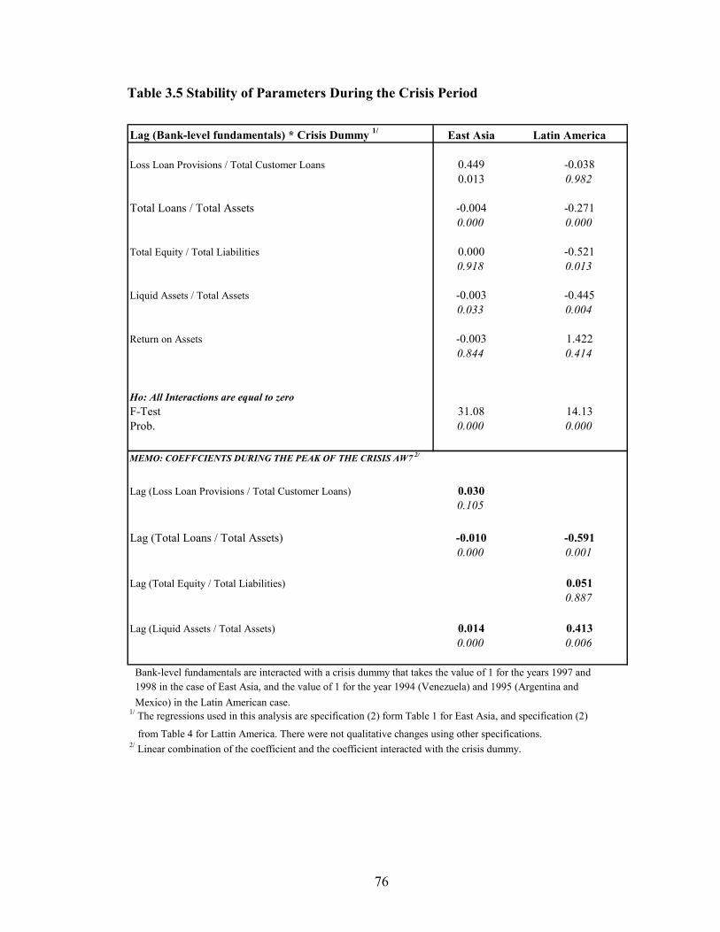
76

Table 3.5 Stability of Parameters During the Crisis Period Lag (Bank-level fundamentals) * Crisis Dummy 1/ East Asia Latin America

Loss Loan Provisions / Total Customer Loans 0.449 -0.0380.013 0.982

Total Loans / Total Assets -0.004 -0.2710.000 0.000

Total Equity / Total Liabilities 0.000 -0.5210.918 0.013

Liquid Assets / Total Assets -0.003 -0.4450.033 0.004

Return on Assets -0.003 1.4220.844 0.414

Ho: All Interactions are equal to zeroF-Test 31.08 14.13Prob. 0.000 0.000

MEMO: COEFFCIENTS DURING THE PEAK OF THE CRISIS AW7 2/

Lag (Loss Loan Provisions / Total Customer Loans) 0.0300.105

Lag (Total Loans / Total Assets) -0.010 -0.5910.000 0.001

Lag (Total Equity / Total Liabilities) 0.0510.887

Lag (Liquid Assets / Total Assets) 0.014 0.4130.000 0.006

Bank-level fundamentals are interacted with a crisis dummy that takes the value of 1 for the years 1997 and 1998 in the case of East Asia, and the value of 1 for the year 1994 (Venezuela) and 1995 (Argentina and Mexico) in the Latin American case.1/ The regressions used in this analysis are specification (2) form Table 1 for East Asia, and specification (2)

from Table 4 for Lattin America. There were not qualitative changes using other specifications.2/ Linear combination of the coefficient and the coefficient interacted with the crisis dummy.

77

Table 3.6 Percentage of Variance Explained by Bank-Level Fundamentals East Asia ALL ESTIMATION PERIOD PEAK OF THE CRISIS

Total Equity / Total Equity /Specification including: Total Assets Total Liabilities Total Liab. + OBS Total Assets Total Liabilities Total Liab. + OBS

Net Foreign Liab ilities 39.02 38.20 35.46 21.55 21.41 20.77

Liquidity outside the FI 34.72 34.16 30.45 21.55 21.49 20.83

AVERAGE 36.87 36.18 32.96 21.55 21.45 20.80

Latin America ALL ESTIMATION PERIOD PEAK OF THE CRISISTotal Equity / Total Equity /

Specification including: Total Assets Total Liabilities Total Assets Total Liabilities

Net Foreign Liab ilities 32.02 31.87 22.18 23.06

Liquidity outside the FI 41.15 41.04 21.89 22.77

AVERAGE 36.59 36.46 22.03 22.92

Figures indicate the percentage of the adjusted R-squared explained by specif ic fundamentals, once the f ixed effects and time dummies have been removed.

A first regression is run w ith macroeconomic and potential contagion variables, then I add specific fundamentals and compute the percentage increase in the

adjusted R-squared.

78

Table 3.7 GMM Estimation (EA: 1994-1999; LA: 1992-1996)

Dependent Variable: Growth Rate of Real Deposits1/

East Asia Latin America(1) (2) (3) (4) (5)

Lag (Growth Rate of Real Deposits) -0.548 *** -0.546 *** -0.543 *** -0.323 *** -0.310 ***0.000 0.000 0.000 0.000 0.000

Lag (Loss Loan Provisions / Total Loans) 0.000 0.000 0.000 -2.316 *** -2.030 ***

0.928 0.970 0.981 0.000 0.005

Lag (Total Loans / Total Assets) -0.008 *** -0.008 *** -0.008 *** -0.124 ** -0.044 *0.000 0.000 0.000 0.021 0.064

Lag (Total Equity / Total Assets) 0.010 *** 0.459 **0.000 0.015

Lag (Total Equity / Total Liabilities) 0.008 *** 0.244 **0.000 0.017

Lag (Total Equity / Total Liabilities + Off-Balance) 0.008 ***0.000

Lag (Liquid Assets / Total Liabilities) 0.012 *** 0.012 *** 0.012 *** 0.368 ** 0.459 ***0.000 0.000 0.000 0.012 0.000

Lag (Return on Assets) 0.002 0.003 0.005 0.104 0.1170.713 0.593 0.309 0.150 0.129

Lag (Total Assets) -0.013 *** -0.013 *** -0.013 *** 0.037 *** 0.319 ***0.000 0.000 0.000 0.000 0.000

Liquidity outside the Bank 2/ 0.003 0.003 0.004 1.793 *** 1.690 ***0.455 0.380 0.285 0.000 0.000

Real Exchange Rate volatility 3/ -0.001 ** -0.001 *** -0.001 *** -0.229 *** -0.207 ***0.014 0.008 0.009 0.005 0.009

GDP variation 4/ 0.011 *** 0.011 *** 0.011 *** 0.335 *** 0.338 ***0.000 0.000 0.000 0.000 0.000

No. Obs. 760 760 760 493 493F-Model 205.33*** 207.70*** 216.92*** 255.44*** 273.02***F- Bank-Fundamentals / excluding bank size 59.42*** 60.35*** 65.88*** 18.75*** 29.07***

1/ Significance levels are below the coefficients in italics. Robust standard errors-White correction for heteroskedasticity are calculated. ***, **, * indicate significance levels at 1, 5 and 10 percent. Regressions include only crisis countries in East Asia and Latin America.2/ Total amount of liquidity relative to total deposits outside the bank, i.e., the amount of cash in vaults in the rest of banks in the system (the summation over the n-1 banks) over the total amount of deposits in the rest of banks in the system (the summation over the n-1 banks).3/ The standard deviation of the monthly percentage variation of the real exchange rate index.

79

Appendices

Appendix I: Description of the Logit and Survival Time Model

A. Logit Model A qualitative response model is used in order to estimate the unconditional probability of

the occurrence of distress as a function of a vector of explanatory variables, X, and a

vector of unknown parameters, θ. The specific model is:

Pr(Yi=1) = F[H(Xi, θ)]

Where:

Y is the dependent variable which takes the value of one if the financial institution has

experienced distress and zero otherwise;

F is the probability function, which has a logistic functional form, giving rise to the logit

model:

H = θ0 + Σj=1 θj Xij

X is the vector of explanatory variables for the i-th individual financial institution; and θ

is the vector of parameters to be estimated. The basic equation of the logit model to be

estimated can be written as:

Pr(Y=1) = F[H(X, θ )] = x

x

ee

'

'

1 β

β

+

80

I use as explanatory variables CAMEL-type variables associated with asset quality (the

loan loss provisions to total loans ratio and the total loans to assets ratio), solvency (the

total equity to total assets or liabilities ratio), liquidity (the liquid assets to total liabilities

ratio), and profitability (return on assets). Also, I include the logarithm of total assets to

proxy for the size of the financial institution. These variables are measured as of

December 1996 for East Asia, September 1994 for Argentina and Mexico, December

1993 for Venezuela, and December 1994 for Chile, Colombia and Peru. In addition, I

include country dummies.

B. Survival Time Model Given the question, what is the likelihood that an event will end the “next period”? The

central concept is occupied not by the unconditional probability of an event taking place,

but of its conditional probability. Survival time analysis allows us to determine the

factors that explain the duration of a given state-in our case, the state of no distress. This

duration is subject to random variations, and they form a distribution, which is generally

characterized by three mathematically equivalent functions: the survival function, the

probability density function, and the hazard function.

The probability distribution of duration can be specified by the distribution function F(t)=

Pr(T<t). The corresponding density function is f(t) = dF(t)/dt. In this context, the survivor

function is given by:

S(t) = 1 – F(t) = Pr(T≥t)

81

Giving the upper tail area of the distribution. The hazard function is:

Λ(t) = f(t) / S(t)

Which is the instantaneous rate of leaving the state of no-distress per unit of period at t54.

The common distributions used in order to derive the hazard function are: exponential,

Weibull, log-logistic and log-normal.

When we introduce explanatory variables, the effect of regressors is to multiply the

hazard function itself by a scale factor (proportional hazard specification). The

interpretation of the coefficients of the explanatory variables depends on the

specification, and the sign of the coefficients indicates the direction of their effect on the

conditional probability.

In the proportional hazard specification, the hazard function, which depends on a vector

of explanatory variables X with unknown coefficients β and Λ0 λ, is factored as:

Λ (t, X, β, Λ0) = Φ (X, β) Λ0(t)

54 A precise definition in terms of probabilities is:

Λ(t) = lim Pr(t ≤ T < t +h | T ≥ t) / h, as h goes to 0. i.e., the conditional probability that a FI that

has occupied the state of no-distress for a time t leaves it in the short interval of length dt after t.

82

Where Λ0 is the “baseline” hazard corresponding to Φ(.) =155. In this specification the

effect of explanatory variables is to multiply the hazard Λ0 by a factor Φ which does not

depend on duration t.

A general specification of Φ is:

Φ (X, β) = exp(X’β)

So, the hazard function takes the following form:

Λ (t, X, β, Λ0) = exp(X’β) Λ0(t)

In the case of a Weibull distribution, which is used in our estimations, the “baseline”

hazard assumes that Λ0(t) = ptp-1, where p is the shape of the parameter to be estimated

from the data. A particular case of the Weibull function is the exponential hazard in

which p=1.

I use the same set of CAMEL-type variables, market-based indicators, and size of the

financial institutions as in the cross-sectional logit estimation. In addition, I include

banking system variables, liquidity outside the financial institution and net foreign

liabilities, and macroeconomic variables, the real exchange rate volatility, GDP growth,

55 “It is common, and sensible, practice to measure the regressors so that Φ(.) =1 at the mean

value of the regressors. Then Λ has an interpretation as the hazard function for the mean

individual in the sample” (Kiefer, 1988, p. 664).

83

and a measure of the stock market. Banking system and macroeconomic variables are

defined in the next section.

84

Appendix II: Description of Data Sample Table II.1 BankScope Sample as of end 1996: Overview of the Financial System

Category Indonesia Korea Malaysia Philippines Thailand Commercial Banks

86 (20) 27 (1) 41 (14) 31 (7) 15 (0)

Other Financial Institutions

3 (0) 28 (0) 33 (0) 5 (0) 26 (1)

Total 89 (20) 55 (1) 74 (14) 36 (7) 41 (1) Numbers in (.) indicate the number of foreign-owned financial institutions. Source: BankScope.

Table II.2 Coverage of the BankScope Sample as of end 1996: In terms of Assets (%)

Category Indonesia Korea Malaysia Philippines Thailand Commercial Banks

94.7 99.0 100 88.0 100

Other Financial Institutions

58.0 58.7 62.5 60.2 89.6

Source: BankScope and countries’ Central Bank statistics.

Table II.3 Coverage of the BankScope Sample as of end 1996: In terms of Number of Financial Institutions (%)

Category Indonesia Korea Malaysia Philippines Thailand Commercial Banks

86 (35%) 27 (34%) 37 (100%) 31 (63%) 15 (100 %)

Other Financial Institutions

3 (2%) 28 (49%) 31 (55%) 5 (5%) 26 (27%)

Source: BankScope and countries’ Central Bank statistics.

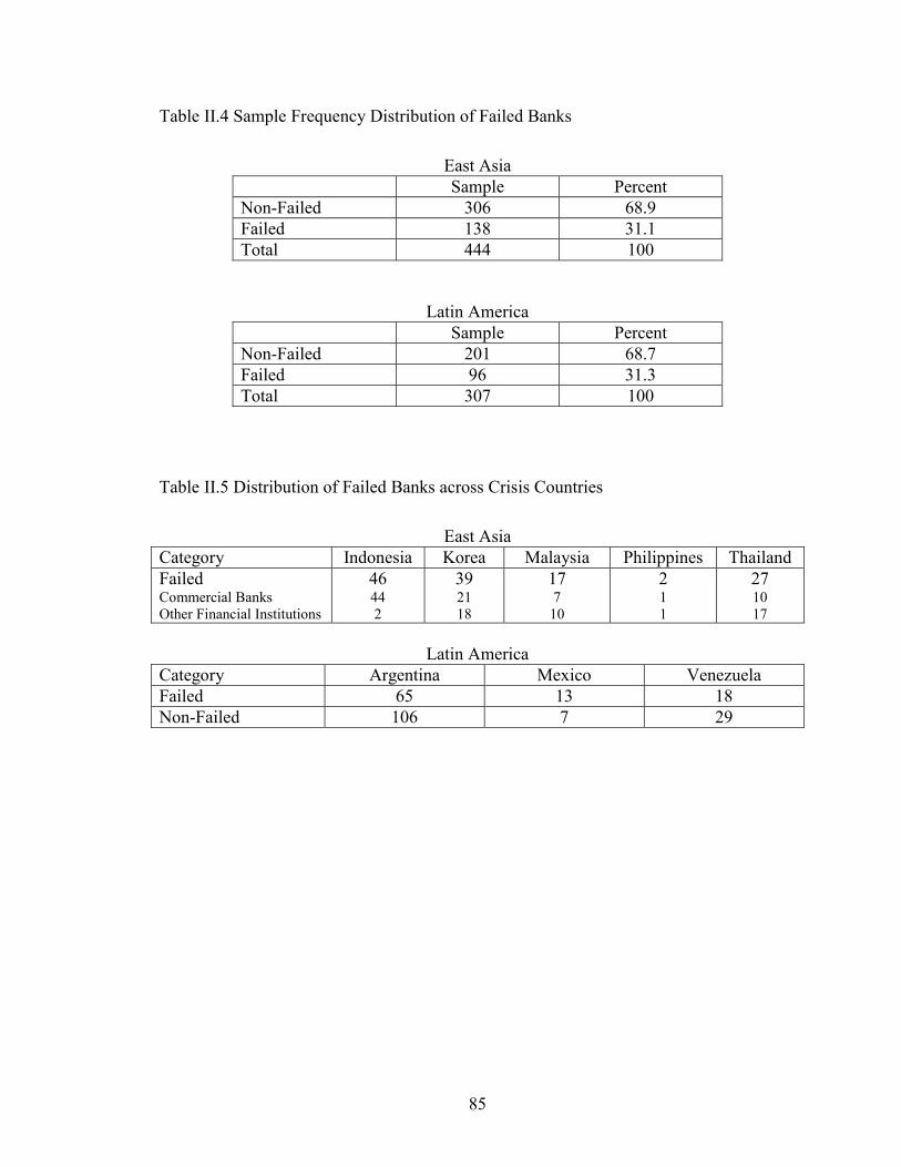
85

Table II.4 Sample Frequency Distribution of Failed Banks

East Asia

Sample Percent Non-Failed 306 68.9 Failed 138 31.1 Total 444 100

Latin America Sample Percent Non-Failed 201 68.7 Failed 96 31.3 Total 307 100

Table II.5 Distribution of Failed Banks across Crisis Countries

East Asia Category Indonesia Korea Malaysia Philippines Thailand Failed Commercial Banks Other Financial Institutions

46 44 2

39 21 18

17 7

10

2 1 1

27 10 17

Latin America

Category Argentina Mexico Venezuela Failed 65 13 18 Non-Failed 106 7 29

86

Appendix III: List of Failed Financial Institutions Failure Code:

1. The financial institution was recapitalized by either the Central Bank or an agency specifically created to tackle the crisis; and/or required a liquidity injection from the Monetary Authority.

2. The financial institution’s operations were temporally suspended (“frozen”)

by the Government;

3. The Government closed the financial institution.

4. The financial institution was absorbed or acquired by another financial institution;

87

Date of Failure Failure Code Bank Name CountryNov-97 3 Andromeda Bank INDONESIAMar-99 3 Bank Arya Panduarta INDONESIAMar-99 3 Bank Asia Pacific - ASPAC Bank INDONESIAMar-99 3 Bank Bahari INDONESIAMar-99 4 Bank Bali INDONESIAMar-99 3 Bank BIRA - Bank Indonesia Raya INDONESIAMar-99 1 Bank Bukopin INDONESIAJan-98 4 Bank Bumi Daya (Persero) PT INDONESIA

Aug-98 2 Bank Central Asia INDONESIAMar-99 3 Bank Central Dagang INDONESIAMar-99 3 Bank Dagang Dan Industri INDONESIAJan-98 4 Bank Dagang Negara (Persero) INDONESIA

Aug-98 2 Bank Danamon Indonesia Tbk INDONESIAMar-99 2 Bank Duta INDONESIAApr-98 2 Bank Ekspor Impor Indonesia - BankExim INDONESIAMar-99 3 Bank First Indonesian Finance and Investments Corporation - Ficorinvest Bank INDONESIAMar-99 1 Bank Internasional Indonesia Tbk INDONESIAMar-99 3 Bank Lautan Berlian INDONESIAMar-99 1 Bank Lippo Tbk. INDONESIAMar-99 3 Bank Mashill Utama INDONESIAAug-98 3 Bank Modern INDONESIAApr-98 2 Bank Nasional INDONESIADec-98 1 Bank Negara Indonesia (Persero) - Bank BNI INDONESIAApr-98 2 Bank Nusa Internasional INDONESIAMar-99 3 Bank Papan Sejahtera INDONESIADec-98 4 Bank Pembangunan Indonesia (Persero) - BAPINDO INDONESIAMar-99 1 Bank Prima Express INDONESIAMar-99 3 Bank Putra Surya Perkasa INDONESIADec-98 1 Bank Rakyat Indonesia INDONESIAMar-99 2 Bank Rama INDONESIAMar-99 3 Bank Sahid Gajah Perkasa INDONESIAApr-98 3 Bank Subentra INDONESIAApr-98 3 Bank Surya INDONESIAAug-98 2 Bank Tiara Asia INDONESIAAug-98 3 Bank Umum Nasional INDONESIAMar-99 3 Bank Umum Servitia INDONESIAMar-99 1 Bank Universal INDONESIAMar-99 3 Hastin Internasional Bank INDONESIAMar-99 2 JayaBank International INDONESIAMar-99 3 Kharisma Bank INDONESIAMar-99 1 PT Bank Niaga Tbk INDONESIANov-97 3 Sejahtera Bank Umum - Bank SBU INDONESIAMar-99 2 Tamara Bank INDONESIAApr-98 3 Bank Pelita INDONESIAAug-98 2 Privat Development Finance Company of Indonesia - Bank PDFCI INDONESIA

88

Date of Failure Failure Code Bank Name CountryJan-99 4 Boram Bank KOREA REP. OFApr-99 4 Chohung Bank KOREA REP. OFJun-98 3 Chung Chong Bank Ltd. (The) KOREA REP. OFApr-99 4 Chungbuk Bank Ltd KOREA REP. OFJan-99 4 Commercial Bank of Korea KOREA REP. OFJun-98 3 Daedong Bank KOREA REP. OFJun-98 3 Donghwa Bank KOREA REP. OFJun-98 3 Dongnam Bank KOREA REP. OF

May-99 1 H&CB KOREA REP. OFMay-99 1 Hana Bank KOREA REP. OF

Jan-99 4 Hanil Bank KOREA REP. OFJun-99 1 Industrial Bank of Korea KOREA REP. OFSep-99 4 Kangwon Bank KOREA REP. OF

May-99 1 Kookmin Bank (Old) KOREA REP. OFMay-99 1 Koram Bank KOREA REP. OF

Jan-98 2 Korea First Bank KOREA REP. OFDec-98 4 Korea Long Term Credit Bank KOREA REP. OFJan-98 3 Kyungki Bank Ltd. KOREA REP. OFJan-98 2 Seoul Bank KOREA REP. OF

May-99 1 Shinhan Bank KOREA REP. OFDec-97 3 Coryo Merchant Bank KOREA REP. OFDec-97 3 Daehan Investment Banking Corp. KOREA REP. OFJun-99 1 Export-Import Bank of Korea KOREA REP. OFDec-97 3 Gyongnam Merchant Banking Corporation KOREA REP. OFDec-97 3 H&S Merchant Banking Corporation KOREA REP. OFDec-97 3 Hansol Merchant Bank KOREA REP. OFDec-97 3 Hanwha Merchant Bank KOREA REP. OFFeb-99 4 Hyundai International Merchant Bank HIMB KOREA REP. OF

1999 4 Hyundai Securities Co. Ltd. KOREA REP. OFJun-99 1 Korea Development Bank KOREA REP. OFDec-98 4 Korea International Merchant Bank KOREA REP. OFJul-99 4 LG Merchant Banking Corporation - LGMB KOREA REP. OF

Dec-97 3 Nara Banking Corporation KOREA REP. OFJul-99 3 National Livestock Cooperatives Federation KOREA REP. OF

Dec-97 3 Saehan Merchant Banking Corp. KOREA REP. OFDec-97 3 Samyang Merchant Bank KOREA REP. OFDec-97 3 Shinhan Investment Bank KOREA REP. OFOct-98 1 AmBank Group MALAYSIAJun-99 4 Bank Bumiputra Malaysia Berhad MALAYSIA

Nov-98 1 BSN Commercial Bank (Malaysia) Berhad MALAYSIAJun-97 4 Chung Khiaw Bank (Malaysia) Bhd MALAYSIAOct-98 1 Oriental Bank Berhad MALAYSIA

Nov-98 1 RHB Bank Berhad MALAYSIANov-98 1 Sabah Bank Berhad MALAYSIANov-98 4 AMFB Holdings Berhad MALAYSIA

89

Date of Failure Failure Code Bank Name CountryNov-98 1 AMMB Holdings Berhad MALAYSIANov-98 1 Arab-Malaysian Merchant Bank Berhad MALAYSIADec-99 4 BSN Merchant Bank BHD MALAYSIAJun-99 4 Hock Hua Finance Berhad MALAYSIAJan-99 4 Multi-Purpose Finance Berhad MALAYSIAJan-98 4 RHB Finance Berhad MALAYSIA

Nov-98 1 Southern Investment Bank Berhad MALAYSIA1999 4 TA Enterprise Berhad MALAYSIA

Nov-98 1 United Merchant Group Bhd. MALAYSIANov-98 1 Utama Merchant Bank Berhad MALAYSIAJun-99 4 Philippine Commercial International Bank - PCIBank PHILIPPINESJul-98 3 Mindanao Development Bank PHILIPPINES

Aug-98 3 Bangkok Bank of Commerce Public Company Limited THAILANDJan-98 2 Bangkok Metropolitan Bank Public Company Limited THAILANDDec-98 1 Bank of Asia Public Company Limited THAILANDAug-98 2 Bankthai Public Company Limited THAILANDJan-98 4 DBS Thai Danu Bank Public Company Limited THAILANDFeb-98 2 First Bangkok City Bank THAILANDFeb-98 2 Siam City Bank Public Company Limited THAILANDDec-98 1 Siam Commercial Bank Public Company Limited THAILANDApr-99 4 Standard Chartered Nakornthon Bank THAILANDAug-98 2 UOB Radanasin Bank Public Company Limited THAILANDApr-99 1 Asia Credit Public Company Limited THAILANDJun-97 3 CMIC Finance and Security PCL THAILAND

Aug-98 2 Dhana Siam Finance & Securities THAILANDJun-97 3 Finance One Public Company Limited THAILANDJun-97 3 General Finance and Securities Ltd. THAILAND

Aug-98 2 IFCT Finance and Securities PCL THAILANDJun-97 3 ITF Finance and Securities PCL THAILAND

Aug-98 4 Krungthai Thanakit PCL THAILANDAug-97 3 Multi-Credit Corporation of Thailand PCL THAILANDMay-98 2 Nava Finance & Securities Public Company Limited THAILANDAug-97 3 SCF Finance and Securities PCL THAILANDAug-97 3 Siam City Credit Finance and Securities PCL THAILANDMay-99 1 Siam Industrial Credit Public Company Limited (The) THAILANDAug-97 3 SITCA Investment and Securities PCL THAILANDAug-97 3 SRI Dhana Finance and Securities PCL THAILANDAug-97 3 Union Asia Finance Public Co. Ltd. THAILANDAug-97 3 Wall Street Finance and Securities PCL THAILAND

90

Date of Failure Failure Code Bank Name CountryDec-95 4 Banesto Banco Shaw ARGENTINAJul-96 4 Banco Popular Argentina SA ARGENTINAJan-97 4 Banco Frances del Rio de la Plata SA ARGENTINADec-96 4 Banco Cooperativo de Caseros Limitado ARGENTINAJul-96 4 The Chase Manhatten Bank, NA ARGENTINA

Aug-96 4 Banco de San Juan SA ARGENTINASep-96 4 Banco Tornquist SA ARGENTINA

May-95 4 Banco Cooperativo de la Plata Ltdo. ARGENTINADec-97 3 Banco Credito Provincial ARGENTINADec-96 4 Banco de Credito Comercial SA ARGENTINAFeb-95 4 Banco de Entre Rios SEM ARGENTINAJul-96 4 Banco de la Provincia de Tucumán. ARGENTINAJul-95 4 Banco Monserrat SA ARGENTINA

Aug-98 4 Banco Rio de la Plata SA ARGENTINAAug-96 4 Banco de Prevision Social SA ARGENTINANov-95 4 Banco Municipal de Parana SEMICFAI ARGENTINAApr-96 4 Banco Commercial del Tandil SA ARGENTINA

May-95 4 Banco Cooperativo del Este Argentino Ltdo. ARGENTINAMar-95 4 Banco de Coronel Dorrego SA ARGENTINA

Jul-95 4 Banco de Junin SA ARGENTINANov-95 4 Banco de Olavarria SA ARGENTINAMar-95 4 Banco Rural (Sunchales) CL ARGENTINAMay-97 2 Nuevo Banco de Azul SA ARGENTINA

Jul-96 4 Banco Popular Financiero SA ARGENTINAApr-97 4 Banco Union Commercial e Industrial CL ARGENTINA

May-95 2 Banco del Noroeste CL ARGENTINAJul-95 3 Banco Federal Argentino ARGENTINA

Mar-96 4 Banco Interfinanzas SA ARGENTINAFeb-95 3 ACISO Banco CL ARGENTINA

May-97 4 Banco Platense SA ARGENTINAMay-95 4 Banco San Jose CL ARGENTINA

Jul-95 4 Banco Cooperative Nicolas Levalle Ltdo ARGENTINAApr-95 4 Banco del Ibera SA ARGENTINAApr-95 4 Banco Coinag CL ARGENTINA

May-95 4 Banco Nucleo CL ARGENTINAMay-95 4 Banco de las Comunidades CL ARGENTINAApr-95 4 Banco Noar CL ARGENTINAJul-95 4 Banco Horizonte CL ARGENTINA

Jun-95 4 Banco Aliancoop CL ARGENTINAFeb-95 4 Banco Nueva Era CL ARGENTINAJun-95 4 Banco VAF CL ARGENTINAApr-95 4 Banco Independcia CL ARGENTINAAug-95 3 Banco Integrado Departmental CL ARGENTINAJun-95 4 Banco C.E.S CL ARGENTINAFeb-95 3 Banco de la Ribera CL ARGENTINAJul-95 4 Banco Meridional CL ARGENTINA

Apr-95 4 Banco de los Arroyos CL ARGENTINA

91

Date of Failure Failure Code Bank Name CountryJun-95 4 Banco Carlos Pelligrini CL ARGENTINAJun-95 4 Banco Nordecoop CL ARGENTINAJun-95 4 Banco Local CL ARGENTINAMar-97 4 Banco Coopesur CL ARGENTINAMar-95 3 Banco Feigin SA ARGENTINAMay-95 4 Banco Asfin SA ARGENTINAMay-95 4 Banco Provencor SA ARGENTINAFeb-97 4 Banco Liniers Sudamericano SA ARGENTINAFeb-96 4 Banco Baires ARGENTINAMar-96 4 Banco UNB SA ARGENTINA

Jul-95 4 Banco Caudal SA ARGENTINAJul-95 4 Banco del Fuerte SA ARGENTINA

Feb-95 3 Banco Multicredito SA ARGENTINAApr-95 3 Banco Austral SA ARGENTINANov-94 3 Banco Extrader SA ARGENTINANov-96 4 Banco de la Cuenca del Plata ARGENTINANov-94 4 Banco del Chaco SEM ARGENTINADec-95 4 Banco de la Provincia de Formosa ARGENTINAJan-96 4 Banco de la Provincia de Missiones ARGENTINA

Mar-96 4 Banco de la Provincia de Rio Negro ARGENTINAMar-96 4 Banco Provincial de Salta. ARGENTINAAug-96 4 Banco de la Provincia de San Luis ARGENTINASep-96 4 Banco de la Provincia de Santiago del Estero ARGENTINANov-96 4 Banco de Mendoza SA ARGENTINA

1995 2-4 COMERMEX MEXICO1995 2-4 Mexicano MEXICO1995 2-4 M. Probursa MEXICO1995 2-4 Centro MEXICO1995 2-4 Confia MEXICO1995 2-4 Banpais MEXICO1995 2-4 Oriente MEXICO1995 2-4 Obrero MEXICO

Jun-94 3 Maracaibo VENEZUELAAug-94 2 Venezuela VENEZUELAFeb-95 1 Union VENEZUELAJan-94 3 Latino VENEZUELAJun-94 3 Metropolitano VENEZUELAFeb-95 3 Italo Venezolano VENEZUELAJun-94 3 La Guaira VENEZUELAJun-94 3 Construccion VENEZUELASep-94 2 Consolidado VENEZUELAJun-94 3 Bancor VENEZUELADec-94 3 Progreso VENEZUELAFeb-95 3 Principal VENEZUELANov-95 3 Andino Venezolano VENEZUELAJun-94 3 Barinas VENEZUELAJun-94 3 Amazonas VENEZUELAFeb-95 3 Profesional VENEZUELAJan-95 3 Empresarial VENEZUELA

92

Appendix IV: Robustness Check Excluding Mergers and Acquisitions of the Definition of Failure

Table IV.1 Mean Tests between Non-Failed FIs and FIs Mergered or Acquired

I. Asset Quality

East Asia Latin AmericaVARIABLE NON-FAILED M&A NON-FAILED M&A

Loan Loss Provisions / Total Equity 3.66 4.90** 6.85 7.81Loan Loss Provisions / Total Loans 0.61 0.54 1.76 1.08Loan Loss Reserves / Total Equity 15.17 21.32**Loan Loss Reserves / Total Loans 2.39 2.38Loans / Total Assets 62.53 68.22* 53.37 69.23******, **, * indicate significant differences between non-failed and M&A financial institutions at 1, 5 and 10 percent.

II. SolvencyEast Asia Latin America

VARIABLE NON-FAILED M&A NON-FAILED M&ATotal Equity / Total Assets 13.77 8.37*** 19.78 15.24**Total Equity / Total Liabilities 14.33 9.45*** 19.74 17.51Total Equity / (Total Liabilities + Off-Balance items) 12.33 8.24******, **, * indicate significant differences between non-failed and M&A financial institutions at 1, 5 and 10 percent.

III. LiquidityEast Asia Latin America

VARIABLE NON-FAILED M&A NON-FAILED M&ALiquid Assets / Total Assets 21.45 17.54* 26.08 16.62***Liquid Assets / Total Liabilities 23.48 19.15* 24.43 19.45******, **, * indicate significant differences between non-failed and M&A financial institutions at 1, 5 and 10 percent.

IV. ProfitabilityEast Asia Latin America

VARIABLE NON-FAILED M&A NON-FAILED M&AReturn on Assets 1.60 0.99*** 1.08 -0.18******, **, * indicate significant differences between non-failed and M&A financial institutions at 1, 5 and 10 percent.

V. Market Based IndicatorsEast Asia Latin America

VARIABLE NON-FAILED M&A NON-FAILED M&A

Growth Rate of Deposits 16.28 17.68 13.03 14.19Loans Interest Rate 14.81 12.62*** 18.62 21.98**Deposits Interest Rate 8.92 9.13 9.20 8.76Spread 6.92 7.11 11.34 13.85******, **, * indicate significant differences between non-failed and M&A financial institutions at 1, 5 and 10 percent. The sample of countries for East Asia includes Hong Kong, Indonesia, Korea, Malaysia, Philippines, Singapore, Taiwan, and Thailand. For Latin America, the sample includes Argentina, Chile, Colombia, Mexico, Peru, and Venezuela.

93

Table IV.2 Cross-Sectional Logit Estimation for East Asia

(Marginal Effects) 1/

(1) (2) (3)

Loan Loss Provisions / Total Loans -0.009 *** -0.008 *** -0.007 ***0.008 0.011 0.023

Total Loans / Total Assets 0.000 0.000 0.0000.959 0.964 0.987

Total Equity / Total Assets -0.025 ***0.000

Total Equity / Total Liabilities -0.019 ***0.000

Total Equity / (Total Liab. + OBS.) -0.015 ***0.002

Liquid Assets / Total Liabilities -0.005 * -0.005 * -0.0040.081 0.079 0.124

Return on Assets -0.090 *** -0.099 *** -0.104 ***0.003 0.002 0.001

Log (Total Assets) -0.053 -0.055 -0.0240.562 0.562 0.806

Indonesia 0.805 *** 0.806 *** 0.827 ***0.000 0.000 0.000

Korea 0.700 *** 0.700 *** 0.723 ***0.000 0.000 0.000

Malaysia 0.566 *** 0.569 *** 0.585 ***0.010 0.000 0.013

Philippines 0.525 0.527 0.4520.128 0.121 0.201

Thailand 0.863 *** 0.861 *** 0.856 ***0.000 0.000 0.000

No. Obs. 335 342 337Wald Chi2 89.72 90.86 92.66Prob > Chi2 0.00 0.00 0.00

The sample of financial institutions (FIs) is divided between failed and non-failed FIs. A financial institution is considered to have

failed If it falls in any of the following categories: (i) The financial institution was recapitalized by either the Central Bank or an

agency specifically created to tackle the crisis or by a strategic investor; and/or required a liquidity injection from the Monetary,

(ii) The financial institution’s operations were temporally suspended (“frozen”) by the Government, (iii) The Government closed

the financial institution.1/ The estimation was done including crisis (Indonesia, Korea, Malaysia, Philippines, and Thailand) and non-crisis countries

(Hong Kong, Singapore, and Taiwan) in East Asia. The dependent variable takes the value of 1 if the financial institution (FI)

falls in the definition of failure given in (1) during the period Jan. 97-Jun. 99, and zero otherwise.

Micro-level bank fundamentals, including the size of the FI, are measured as of December 1996. A constant term was

included in the initial estimation so the marginal effect of country dummies have to be interpreted relative to non-crisis countries.3/ Marginal effects are reported rather than the coefficients. The significance level is reported in italics below the marginal

effects. The Z-stat are based on robust (Huber and White) standard errors which account for correlated observations in grouped

data. ***, **, * indicate significance levels at 1, 5 and 10 percent.

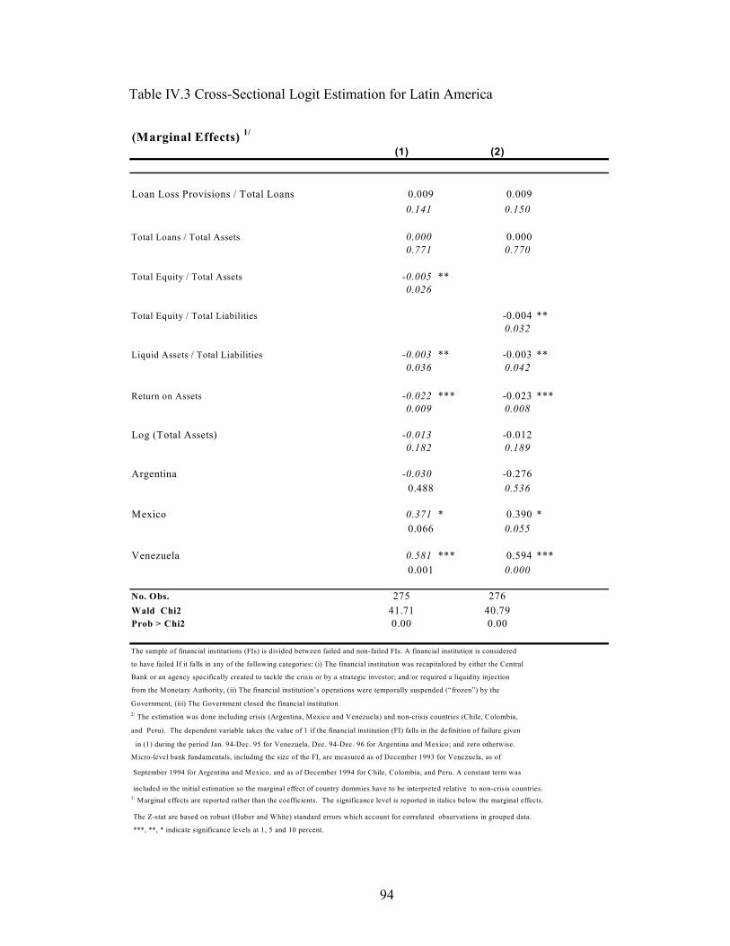
94

Table IV.3 Cross-Sectional Logit Estimation for Latin America

(Marginal Effects) 1/

(1) (2)

Loan Loss Provisions / Total Loans 0.009 0.0090.141 0.150

Total Loans / Total Assets 0.000 0.0000.771 0.770

Total Equity / Total Assets -0.005 **0.026

Total Equity / Total Liabilities -0.004 **0.032

Liquid Assets / Total Liabilities -0.003 ** -0.003 **0.036 0.042

Return on Assets -0.022 *** -0.023 ***0.009 0.008

Log (Total Assets) -0.013 -0.0120.182 0.189

Argentina -0.030 -0.2760.488 0.536

Mexico 0.371 * 0.390 *0.066 0.055

Venezuela 0.581 *** 0.594 ***0.001 0.000

No. Obs. 275 276Wald Chi2 41.71 40.79Prob > Chi2 0.00 0.00

The sample of financial institutions (FIs) is divided between failed and non-failed FIs. A financial institution is considered

to have failed If it falls in any of the following categories: (i) The financial institution was recapitalized by either the Central

Bank or an agency specifically created to tackle the crisis or by a strategic investor; and/or required a liquidity injection

from the Monetary Authority, (ii) The financial institution’s operations were temporally suspended (“frozen”) by the

Government, (iii) The Government closed the financial institution.2/ The estimation was done including crisis (Argentina, Mexico and Venezuela) and non-crisis countries (Chile, Colombia,

and Peru). The dependent variable takes the value of 1 if the financial institution (FI) falls in the definition of failure given

in (1) during the period Jan. 94-Dec. 95 for Venezuela, Dec. 94-Dec. 96 for Argentina and Mexico; and zero otherwise.

Micro-level bank fundamentals, including the size of the FI, are measured as of December 1993 for Venezuela, as of

September 1994 for Argentina and Mexico, and as of December 1994 for Chile, Colombia, and Peru. A constant term was

included in the initial estimation so the marginal effect of country dummies have to be interpreted relative to non-crisis countries.1/ Marginal effects are reported rather than the coefficients. The significance level is reported in italics below the marginal effects.

The Z-stat are based on robust (Huber and White) standard errors which account for correlated observations in grouped data.

***, **, * indicate significance levels at 1, 5 and 10 percent.

95

Appendix V: Description of the Generalized Methods of Moments (GMM) Estimation Generalized-Method-of Moments dynamic panel estimators control for unobserved

country-specific effects, the endogeneity of explanatory variables, time specific effects,

and the use of lagged dependent variables. Consider the following regression equation,

yi,t - yi,t-1 = (α-1) yi,t-1 + β' Xi,t + ηi + εi,t (7)

Where y represents the growth rate of real total deposits of bank i, X represents the set of

explanatory variables (bank level fundamentals lagged one period, banking system and

macroeconomic variables), η is an unobserved country-specific effect, ε is the error term,

and the subscripts i and t represent individual banks and time period, respectively. The

dependent variable in equation (1) is the period’s average growth rate. We can rewrite

equation (7) as a lagged-dependent variable equation as follows,

yi,t = α yi,t-1 + β' Xi,t + ηi + εi,t (8)

The usual method of dealing with the country-specific effect in the context of panel data

has been to first-difference the regression equation (Anderson and Hsiao 1981). In this

way the specific-effect is directly eliminated from the estimation process. First-

differencing equation (8), we obtain

yi,t - yi,t-1 = α (yi,t-1 - yi,t-2) + β' (Xi,t - Xi,t-1) + (εi,t - εi,t-1) (9)

96

The use of instruments is again required to deal with two issues: first, the likely

endogeneity of explanatory variables, X; and, second, the new error term, εi,t - εi,t-1 is

correlated with the differenced lagged dependent variable, yi,t-1 - yi,t-2. This second issue

arises by construction when we difference equation (8). To address this correlation and

the endogeneity problem, Arellano and Bond (1991) propose using the lagged values of

the explanatory variables in levels as instruments.

We would like to relax the assumption that all the explanatory variables are strictly

exogenous (that is, that they are uncorrelated with the error term at all leads and lags).

Relaxing this assumption allows for the possibility of simultaneity and reverse causality,

which are very likely present in growth regressions. We adopt the assumption of weak

exogeneity of the explanatory variables, in the sense that they are assumed to be

uncorrelated with future realizations of the error term. This weaker assumption means

that current explanatory variables may be affected by past and current growth rates but

not by future ones.

Under the assumptions that (a) the error term, ε, is not serially correlated, and (b) the

explanatory variables, X, are weakly exogenous, the following moment conditions apply

to the lagged dependent variable and the set of explanatory variables:

E[yi,t-s * (εi,t - εi,t-1)] = 0 for s ≥ 2; t= 3, ..., T (10)

E[Xi,t-s * (εi,t - εi,t-1)] = 0 for s ≥ 2; t= 3, ..., T (11)

97

Using these moment conditions, Arellano and Bond (1991) propose a two-step GMM

estimator. In the first step, the error terms are assumed to be both independent and

homoskedastic, across countries and over time. In the second step, the residuals obtained

in the first step are used to construct a consistent estimate of the variance-covariance

matrix, thus relaxing the assumptions of independence and homoskedasticity. We refer to

this estimator as the difference estimator.

There are, however conceptual and statistical shortcomings with this estimator.

Conceptually, we would like to study not only the time-series relationship between bank-

level fundamentals and the growth rate of real deposits but also their cross-sectional

relationship, which is eliminated in the case of the simple difference estimator.

Statistically, Alonso-Borrego and Arellano (1996) and Blundell and Bond (1997) show

that when the lagged dependent and the explanatory variables are persistent over time,

lagged levels of these variables are weak instruments for the regression equation in

differences. The instruments' weakness has repercussions on both the asymptotic and

small-sample performance of the difference estimator. As the variables' persistence

increases, the asymptotic variance of the coefficients obtained with the difference

estimator rises (that is, the asymptotic precision of this estimator deteriorates).

Furthermore, Monte Carlo experiments show that the weakness of the instruments

produced biased coefficients in small samples. This bias is exacerbated with the variables'

over time persistence, the importance of the specific-effect, and the smallness of the time

series dimension. To confront these conceptual and statistical concerns, we use

alternative estimators.

98

Blundell and Bond (1997) suggest the use of Arellano and Bover's (1995) system

estimator that-- based on asymptotic and small sample properties-- reduces the potential

biases and imprecision associated with the usual difference estimator. Arellano and Bover

(1995) present an estimator that combines, in a system, the regression in differences with

the regression in levels. The instruments for the regression in differences are the same as

above (i.e., the lagged levels of the corresponding variable), so that, the moment

conditions in equations (10) and (11) apply to this first part of the system. The

instruments for the regression in levels are the lagged differences of the corresponding

variables. These are appropriate instruments under the following additional assumption:

although there may be correlation between the levels of the right-hand side variables and

the country-specific effect in equation (8), there is no correlation between the differences

of these variables and the country-specific effect. This assumption results from the

following stationarity property,

E[yi,t+p * ηi ] = E[yi,t+p * ηi ] (12)

E[Xi,t+p * ηi ] = E[yi,t+q * ηi ] for all p and q

Therefore, the additional moment conditions for the second part of the system (the

regression in levels) are given by the following equations:

E[ (yi,t-s - yi,t-s-1) * (ηi + εi,t)] = 0 for s = 1 (13)

E[ (Xi,t-s - Xi,t-s-1) * (ηi + εi,t)] = 0 for s = 1 (14)

99

Thus, we use the moment conditions presented in equations (10), (11), (13), and (14) and

employ a GMM procedure to generate consistent and efficient estimates of the

parameters of interest (Arellano and Bond, 1991; Arellano and Bover, 1995).

The consistency of the GMM estimator depends on whether lagged values of the growth

rate of real deposits and other explanatory variables are valid instruments in the growth

regression. To address this issue, I consider two specification tests suggested by Arellano

and Bond (1991), Arellano and Bover (1995), and Blundell and Bond (1997). The first is

a Sargan test of over-identifying restrictions, which tests the overall validity of the

instruments by analyzing the sample analog of the moment conditions used in the

estimation process. The second test examines the hypothesis that the error term εi,t is not

serially correlated. In the both the difference regression and the system difference-level

regression we test whether the differenced error term is second-order serially correlated

(by construction, it is likely that this differenced error term be first-order serially

correlated even if the original error term is not).

100

References Arellano, M. and S. Bond (1991), “Some Tests of Specification for Panel data: Monte Carlo Evidence and an Application to Employment Equations,” Review of Economic Studies, 58(2), 277-297. Arellano, M. and O. Bover (1995), “Another Look to Instrumental-Variable Estimation of Error Components Models,” Journal of Econometrics, 68(1), 29-52. Baer, H. and E. Brewer (1994), “Uninsured Deposit as a Source of Market Discipline: Some New Evidence,” Economic Perspectives, Federal Reserve Bank of Chicago (September/October 1986), 23-31. Barth, J., D. Brumbaugh Jr., D. Sauerhaft, and G. H. K. Wang (1985), “Thrift Institution Failures: Causes and Policy Issues,” in Bank Structure and Competition, Conference Proceedings, Federal Reserve Bank of Chicago. Barth, J., G. Caprio, and R. Levine (2001), “Bank Regulation and Supervision: What Works Best?” World Bank Policy Research Paper, No. 2725 (Washington, D.C.: World Bank). Berger, A. (1991), “Market Discipline in Banking,” Proceedings of a Conference on Bank Structure and Competition, Federal Reserve Bank of Chicago. Bhattacharya, S. (1993), “Contemporary Banking Theory,” Journal of Financial Intermediation, 3(1), 2-50. Blundell, R. and S. Bond (1997), “Initial Conditions and Moment Restrictions in Dynamic Panel Data Model,” University College London Discussion Paper, No. 97-07 (University College London). Breuer, Peter (2000), “Measuring Off-Balance Sheet Leverage,” IMF Working Paper, WP/00/202 (Washington, D.C.: International Monetary Fund). Bongini, P., S. Claessens, and G. Ferri (2001), “The Political Economy of Distress in East Asian Financial Institutions,” Journal of Financial Services Research, Vol. 19 No.1 (February) 5-25. Calomiris, C. (1995), “Financial Fragility: Issues and Policy Implications,” Journal of Financial Services Research, 9(3-4), 241-257. Calomiris, C. and G. Gorton (1991), “The Origins of Banking Panics: Models, Facts and Regulation” in Hubbard, ed., Financial Markets and Financial Crisis (University of Chicago Press).

101

Calomiris, C. and Mason, J. (1997), “Contagion and Bank Failures During the Great Depression: The June 1932 Chicago Banking Panic,” American Economic Review, 87 (December) 863-883. Calomiris, C. and Mason, J. (2000), “Causes of U.S. Distress During the Depression,” NBER Working Paper, No. 7919 (Cambridge, MA: National Bureau of Economic Research). Caprio, Gerard Jr., and Daniela Klingebiel. (1996), “Bank Insolvencies: Cross-country Experience,” World Bank Policy Research Paper, No. 1620 (Washington, D.C.: World Bank). Caprio, Gerard Jr., and Daniela Klingebiel. (1999), “Bank Insolvencies: Cross-country Experience,” World Bank. Mimeo. (Washington, D.C.: World Bank). Chang, R. and Velasco, A. (1999), “Liquidity Crisis in Emerging Markets: Theory and Policy.” NBER, Macroeconomics Annual 1999. The MIT Press, Cambridge, MA. Chang, R. and Velasco, A. (2001), “A Model of Financial Crisis in Emerging Markets,” Quarterly Journal of Economics, 116 (2), 445-464. Chari,V. and R. Jagannathan (1988), “Banking Panics, Information and Rational Expectations,” Journal of Finance, 43(3), 749-763. Chinn, M. and Kletzer, K. (2000), “International Capital Inflows, Domestic Financial Intermediation and Financial Crises Under Imperfect Information,” NBER Working Paper, No. 7902 (Cambridge, MA: National Bureau of Economic Research). Cook, D. and L. Spellman (1994), “Repudiation Risk and Restitution Costs: Toward Understanding Premiums on Insured Deposits,” Journal of Money, Credit and Banking 26 (August), 439-459. Corsetti, G., P. Pesenti, and N. Roubini (1998), “What Caused the Asian Currency and Financial Crisis? Part I: A Macroeconomic Overview, in Nouriel Roubini’s website, www.stern.nyu.edu/~nroubini/asia/AsiaHomepage.html. D’Amato, L., E. Grusbisic, and A. Powell (1997), “Contagion, Bank Fundamentals or Macroeconomic Shock? An Empirical Analysis of the Argentine 1995 Banking Problems,” Banco Central de la Republica Argentina, mimeo. Dekle, R. and Kletzer, K. (2001), “Domestic Bank Regulation and Financial Crises: Theory and Empirical Evidence From East Asia,” NBER Working Paper, No. 8322 (Cambridge, MA: National Bureau of Economic Research). Demigurc-Kunt, A. and E. Detragiache (1997), “Determinants of Banking Crisis: Evidence from Developed and Developing Countries,” IMF Working Paper, WP/97/106 (Washington, D.C.: International Monetary Fund).

102

Demigurc-Kunt A. and E. Detragiache (1999), “ Monitoring Banking Sector Fragility: A Multivariate Logit Approach with an application to the 1996-97 banking crisis,” IMF Working Paper, WP/99/147 (Washington, D.C.: International Monetary Fund). Demigurc-Kunt A. and E. Detragiache (2000). “Does Deposit Insurance Increase Banking System Stability?” IMF Working Paper, WP/00/03 (Washington, D.C.: International Monetary Fund). Diamond, D. and P. Dybvig (1983), “Bank Runs, Deposit Insurance, and Liquidity,” The Journal of Political Economy, 91(3), 401-419. Diamond, D. and R. Rajan (2002), “Liquidity Shortages and Banking Crisis,” NBER Working Paper, No. 8937 (Cambridge, MA: National Bureau of Economic Research). Ellis, D. And M. Flannery (1992), “Does the Debt Market Assess Large Banks’ Risk?: Time Series Evidence from Money Center CDS,” Journal of Monetary Economics, 30(3), 481-502. Flannery, M (1998), “Using Market Information in Prudential Bank Supervision: A Review of the U.S. Empirical Evidence,” Journal of Money, Credit and Banking, 30(August), 273-305. Goldberg, L. And S. Hudgins (1986),”Response of Uninsured Depositors to Impending S&L Failure: Evidence of Depositor Discipline,” The Quarterly Review of Economic and Finance 36, 311-325. Gonzalez-Hermosillo, B. (1996), “Banking Sector Fragility and Systemic Sources of Fragility,” IMF Working Paper, WP/96/ 12 (Washington, D.C.: International Monetary Fund). Gonzalez-Hermosillo, B. (1997), “Determinants of Banking System Fragility: A Case Study of Mexico,” IMF Staff Papers, Vol. 44 No. 3 (Washington, D.C.: International Monetary Fund). Gonzalez-Hermosillo, B. (1999), “Determinants of Ex-Ante Banking System Distress: A Macro-Micro Empirical Exploration of Some Recent Episodes,” IMF Working Paper, WP/99/33 (Washington, D.C.: International Monetary Fund). Hannan, T. and G. Hanweck (1988), “Bank Insolvency Risk and the Market for Large Certificates of Deposit,” Journal of Money, Credit and Banking, 20(2), 203-211. Hausmann, R. and Gavin, M. (1996), “The Roots of Banking Crises: The Macroeconomic Context,” in: Banking Crises in Latin America, edited by R. Hausmann and L.Rojas-Suarez.

103

Honohan, P. (1997),”Banking System failures in Developing and Transition Countries: Diagnosis and Prediction,” BIS Working Paper, No. 39, (Basle: Bank of International Settlements). Jacklin, C. and S. Bhattacharya (1988), “Distinguishing Panics and Information Based Bank Runs: Welfare and Policy Implications,” Journal of Political Economy, 96(3), 568-591. Johnston, B., J. Chai, and L. Schumacher (2000), “Assessing Financial System Vulnerabilities,” IMF Working Paper, WP/00/76 (Washington, D.C.: International Monetary Fund). Kaminsky, G.L., Reinhart, C.M. (1999), “The Twin Crises: The Causes of Banking and Balance of Payments Problems,” American Economic Review, 89(3), 473-500.

Kiefer, N. (1988), “Economic Duration Data and Hazard Functions,” Journal of Economic Literature, 26 (June), 646-679.

Laeven, L. (1999), “Risk and Efficiency in East Asian Banks,” World Bank Policy Research Paper, No. 2225 (Washington, D.C.: World Bank).

Lindgren, C-J., T. Baliño, C. Enoch, A-M. Gulde, M. Quintyn, and L. Teo (1999), “Financial Sector Crisis and Restructuring, Lesson from Asia,” IMF Occasional Paper, No. 188 (Washington, D.C.: International Monetary Fund).

Maechler, A. and K. McDill (2003), “Dynamic Deposit Discipline in U.S. Banks,” IMF Working Paper, WP/03/226 (Washington, D.C.: International Monetary Fund). Martin, D. (1977), “Early Warning of Bank Failure,” Journal of Banking and Finance, 1 (November), 249-276.

McKinnon, R.I. and Pill, H. (1997), "Credible Liberalizations and Overborrowing," American Economic Review Vol. 87,189-203.

Minsky, Hyman (1977), ”A Theory of Systemic Fragility,” in: Financial Crises, Institutes and Markets in a Fragile Environment, edited by E. Altman and A. Sametz. Oviedo, P. (2003), “Macroeconomic Risk and Banking Crises in Emerging Markets Countries: Business Fluctuations with Financial Crashes”. Mimeo. Park, S. (1991), “Bank Contagion, Theory and Evidence,” Journal of Financial Services: 123-150. Park, S. and S. Peristiani (1998), “Market Discipline by Thrift Depositors,” Journal of Money, Credit and Banking, Vol. 30, Part 1, 347-64.

104

Radelet, S., and J. Sachs (1998), “The Onset of the East Asian Financial Crisis,” Harvard Institute for International Development. Rojas-Suarez, L. (2001), “Early Warning Indicators of Banking Crises: What Works for Emerging Markets?” Institute of International Economics. Rojas-Suarez, L. (1998),”Rating Banks in Emerging Markets: What Credit Rating Agencies Should Learn From Financial Indicators,” Institute for International Economics. Saunders, A. and B. Wilson (1994), “Contagious Bank Runs: Evidence From the 1929-1933 Period,” Mimeo. Sinkey, J. (1975), “A Multivariate Analysis of the Characteristics of Problem Banks,” Journal of Finance, 30 (March), 21-36. Schmukler, S. and Martinez-Peria, S. (2001), “Do Depositors Punish Banks for “Bad” Behavior? Market Discipline, Deposit Insurance, and Banking Crises,” Journal of Finance, 56(3), 1029-1051. Schumacher, L. (1996), “Bubble or Depositor’s Discipline? A Study of the Argentine Banking Panic (December 1994/May 1995),” Ph.D. Dissertation, University of Chicago. Sundararajan, V. and T. Baliño (1991), ”Issues in Recent Banking Crisis in Developing Countries,” in Banking Crises: Cases and Issues (Washington, D.C.: International Monetary Fund. Velasco, Andres (1987), “Financial Crises and Balance of Payments Crises: A Simple Model of the Southern Cone Experience,” Journal of Development Economics, 27(October), 263-283. Waldo, D. (1985), “Bank Runs, the Deposit-Currency Ratio and the Interest Rate,” Journal of Monetary Economics, 15(May), 260-277. Whalen, G. (1991), “A Proportional Hazard Model of Bank Failure: An Examination of its Usefulness as an Early Warning Tool,” in Economic Review, Federal reserve Bank of Cleveland, Vol. 27, Quarter 1, No. 1.