access from the university of nottingham repositoryeprints.nottingham.ac.uk/40165/1/cinner et al...
TRANSCRIPT

Cinner, Joshua E. and Huchery, Cindy and Macneill, M. Aaron and Graham, Nicholas A.J. and McClanahan, Tim R. and Maina, Joseph and Maire, Eva and Kittinger, John N. and Hicks, Christina C. and Mora, Camilo and Allison, Edward H. and D'Agata, Stephanie and Hoey, Andrew and Feary, David A. and Crowder, Larry and Williams, Ivor D. and Kulbicki, Michel and Vigliola, Laurent and Wantiez, Laurent and Edgar, Graham and Stuart-Smith, Rick D. and Sandin, Stuart A. and Green, Alison L. and Hardt, Marah J. and Beger, Maria and Friedlander, Alan and Campbell, Stuart J. and Holmes, Katherine E. and Wilson, Shaun K. and Brokovich, Eran and Brooks, Andrew J. and Cruz-Motta, Juan J. and Booth, David J. and Chabanet, Pascale and Gough, Charlie and Tupper, Mark and Ferse, Sebastian C.A. and Sumaila, U. Rashid and Mouillot, David (2016) Bright spots among the world’s coral reefs. Nature, 535 (7612). pp. 416-419. ISSN 1476-4687
Access from the University of Nottingham repository: http://eprints.nottingham.ac.uk/40165/1/Cinner%20et%20al%20%20Bright%20spots%20Nature%20final%20submission%20Editorial%20Changes%20Incorporated_without%20Endnote%20and%20ED.pdf
Copyright and reuse:
The Nottingham ePrints service makes this work by researchers of the University of Nottingham available open access under the following conditions.
This article is made available under the University of Nottingham End User licence and may be reused according to the conditions of the licence. For more details see: http://eprints.nottingham.ac.uk/end_user_agreement.pdf

A note on versions:
The version presented here may differ from the published version or from the version of record. If you wish to cite this item you are advised to consult the publisher’s version. Please see the repository url above for details on accessing the published version and note that access may require a subscription.
For more information, please contact [email protected]

1
Bright spots among the world’s coral reefs 1
2
Joshua E. Cinner1,*, Cindy Huchery1, M. Aaron MacNeil1,2,3, Nicholas A.J. Graham1,4, 3
Tim R. McClanahan5, Joseph Maina5,6, Eva Maire1,7, John N. Kittinger8,9, Christina C. 4
Hicks1,4,8, Camilo Mora10, Edward H. Allison11, Stephanie D’Agata5,7,12, Andrew 5
Hoey1, David A. Feary13, Larry Crowder8, Ivor D. Williams14, Michel Kulbicki15, 6
Laurent Vigliola12, Laurent Wantiez 16, Graham Edgar17, Rick D. Stuart-Smith17, 7
Stuart A. Sandin18, Alison L. Green19, Marah J. Hardt20, Maria Beger6, Alan 8
Friedlander21,22, Stuart J. Campbell5, Katherine E. Holmes5, Shaun K. Wilson23,24, 9
Eran Brokovich25, Andrew J. Brooks26, Juan J. Cruz-Motta27, David J. Booth28, 10
Pascale Chabanet29, Charlie Gough30, Mark Tupper31, Sebastian C.A. Ferse32, U. 11
Rashid Sumaila33, David Mouillot1,7 12
13
1Australian Research Council Centre of Excellence for Coral Reef Studies, James 14
Cook University, Townsville, QLD 4811 Australia 15
2Australian Institute of Marine Science, PMB 3 Townsville MC, Townsville, QLD 16
4810 Australia 17
3Department of Mathematics and Statistics, Dalhousie University, Halifax, NS B3H 18
3J5 Canada 19
4Lancaster Environment Centre, Lancaster University, Lancaster, LA1 4YQ, UK 20
5Wildlife Conservation Society, Global Marine Program, Bronx, NY 10460 USA 21
6Australian Research Council Centre of Excellence for Environmental Decisions, 22
Centre for Biodiversity and Conservation Science, University of Queensland, 23
Brisbane St Lucia QLD 4074 Australia 24

2
7MARBEC, UMR IRD-CNRS-UM-IFREMER 9190, Université Montpellier, 34095 25
Montpellier Cedex, France 26
8Center for Ocean Solutions, Stanford University, CA 94305 USA 27
9Conservation International Hawaii, Betty and Gordon Moore Center for Science and 28
Oceans, 7192 Kalaniana‘ole Hwy, Suite G230, Honolulu, Hawai‘i 96825 USA 29
10Department of Geography, University of Hawai‘i at Manoa, Honolulu, Hawai‘i 30
96822 USA 31
11School of Marine and Environmental Affairs, University of Washington, Seattle, 32
WA 98102 USA 33
12Institut de Recherche pour le Développement, UMR IRD-UR-CNRS ENTROPIE, 34
Laboratoire d’Excellence LABEX CORAIL, BP A5, 98848 Nouméa Cedex, New 35
Caledonia 36
13Ecology & Evolution Group, School of Life Sciences, University Park, University 37
of Nottingham, Nottingham NG7 2RD, UK 38
14Coral Reef Ecosystems Division, NOAA Pacific Islands Fisheries Science Center, 39
Honolulu, HI 96818 USA 40
15UMR Entropie, Labex Corail, –IRD, Université de Perpignan, 66000, Perpignan, 41
France 42
16EA4243 LIVE, University of New Caledonia, BPR4 98851 Noumea cedex, New 43
Caledonia 44
17Institute for Marine and Antarctic Studies, University of Tasmania, Hobart, 45
Tasmania, 7001 Australia 46
18Scripps Institution of Oceanography, University of California, San Diego, La Jolla, 47
CA 92093 USA 48
19The Nature Conservancy, Brisbane, Australia 49

3
20Future of Fish, 7315 Wisconsin Ave, Suite 1000W, Bethesda, MD 20814, USA 50
21Fisheries Ecology Research Lab, Department of Biology, University of Hawaii, 51
Honolulu, HI 96822, USA 52
22National Geographic Society, Pristine Seas Program, 1145 17th Street N.W. 53
Washington, D.C. 20036-4688, USA 54
23Department of Parks and Wildlife, Kensington, Perth WA 6151 Australia 55
24Oceans Institute, University of Western Australia, Crawley, WA 6009, Australia 56
25The Israeli Society of Ecology and Environmental Sciences, Kehilat New York 19 57
Tel Aviv, Israel 58
26Marine Science Institute, University of California, Santa Barbara, CA 93106-6150, 59
USA 60
27Departamento de Ciencias Marinas., Recinto Universitario de Mayaguez, 61
Universidad de Puerto Rico, 00680, Puerto Rico 62
28School of Life Sciences, University of Technology Sydney 2007 Australia 63
29UMR ENTROPIE, Laboratoire d’Excellence LABEX CORAIL, Institut de 64
Recherche pour le Développement, CS 41095, 97495 Sainte Clotilde, La Réunion 65
(FR) 66
30Blue Ventures Conservation, 39-41 North Road, London N7 9DP, United Kingdom 67
31Coastal Resources Association, St. Joseph St., Brgy. Nonoc, Surigao City, Surigao 68
del Norte 8400, Philippines 69
32Leibniz Centre for Tropical Marine Ecology (ZMT), Fahrenheitstrasse 6, D-28359 70
Bremen, Germany 71
33Fisheries Economics Research Unit, University of British Columbia, 2202 Main 72
Mall, Vancouver, B.C., V6T 1Z4, Canada 73
74


5
Ongoing declines among the world’s coral reefs1,2 require novel approaches to 77
sustain these ecosystems and the millions of people who depend on them3. A 78
presently untapped approach that draws on theory and practice in human health 79
and rural development4,5 is systematically identifying and learning from the 80
‘outliers’- places where ecosystems are substantially better ('bright spots') or 81
worse ('dark spots') than expected, given the environmental conditions and 82
socioeconomic drivers they are exposed to. Here, we compile data from more 83
than 2,500 reefs worldwide and develop a Bayesian hierarchical model to 84
generate expectations of how standing stocks of reef fish biomass are related to 85
18 socioeconomic drivers and environmental conditions. We then identified 15 86
bright spots and 35 dark spots among our global survey of coral reefs, defined as 87
sites that had biomass levels more than two standard deviations from 88
expectations. Importantly, bright spots were not simply comprised of remote 89
areas with low fishing pressure- they include localities where human populations 90
and use of ecosystem resources is high, potentially providing novel insights into 91
how communities have successfully confronted strong drivers of change. 92
Alternatively, dark spots were not necessarily the sites with the lowest absolute 93
biomass and even included some remote, uninhabited locations often considered 94
near-pristine6. We surveyed local experts about social, institutional, and 95
environmental conditions at these sites to reveal that bright spots were 96
characterised by strong sociocultural institutions such as customary taboos and 97
marine tenure, high levels of local engagement in management, high dependence 98
on marine resources, and beneficial environmental conditions such as deep-99
water refuges. Alternatively, dark spots were characterised by intensive capture 100
and storage technology and a recent history of environmental shocks. Our 101

6
results suggest that investments in strengthening fisheries governance, 102
particularly aspects such as participation and property rights, could facilitate 103
innovative conservation actions that help communities defy expectations of 104
global reef degradation. 105
106

7
Main text 107
Despite substantial international conservation efforts, many of the world's ecosystems 108
continue to decline1,7. Most conservation approaches aim to identify and protect 109
places of high ecological integrity under minimal threat8. Yet, with escalating social 110
and environmental drivers of change, conservation actions are also needed where 111
people and nature coexist, especially where human impacts are already severe9. Here, 112
we highlight an approach for implementing conservation in coupled human-natural 113
systems focused on identifying and learning from outliers - places that are performing 114
substantially better than expected, given the socioeconomic and environmental 115
conditions they are exposed to. By their very nature, outliers deviate from 116
expectations, and consequently can provide novel insights on confronting complex 117
problems where conventional solutions have failed. This type of positive deviance, or 118
‘bright spot’ analysis has been used in fields such as business, health, and human 119
development to uncover local actions and governance systems that work in the 120
context of widespread failure10,11, and holds much promise in informing conservation. 121
122
To demonstrate this approach, we compiled data from 2,514 coral reefs in 46 123
countries, states, and territories (hereafter ‘nation/states’) and developed a Bayesian 124
hierarchical model to generate expected conditions of how standing reef fish biomass 125
(a key indicator of resource availability and ecosystem functions12) was related to 18 126
key environmental variables and socioeconomic drivers (Fig. 1; Extended Data Tables 127
1-4; Extended Data Figures 1-3; Methods). Drawing on a broad body of theoretical 128
and empirical research in the social sciences13-15 and ecology2,6,16 on coupled human-129
natural systems, we quantified how reef fish biomass (Fig. 1a) was related to distal 130
social drivers such as markets, affluence, governance, and population (Fig. 1b,c), 131

8
while controlling for well-known environmental conditions such as depth, habitat, and 132
productivity (Fig. 1d) (Extended Data Table 1, Methods). In contrast to many global 133
studies of reef systems that are focused on demonstrating the severity of human 134
impacts6, our examination seeks to uncover potential policy levers by highlighting the 135
relative role of specific social drivers. A key and significant finding from our global 136
analysis is that our metric of potential interactions with urban centres, called market 137
gravity17 (Methods), more so than local or national population pressure, management, 138
environmental conditions, or national socioeconomic context, had the strongest 139
relationship with reef fish biomass (Fig.1). Specifically, we found that reef fish 140
biomass decreased as the size and accessibility of markets increased (Extended Data 141
Fig. 1b). Somewhat counter-intuitively, fish biomass was higher in places with high 142
local human population growth rates, likely reflecting human migration to areas of 143
better environmental quality18-a phenomenon that could result in increased 144
degradation at these sites over time. We found a strong positive, but less certain 145
relationship (i.e. a high standardized effect size, but only >75% of the posterior 146
distribution above zero) with the Human Development Index, meaning that reefs 147
tended to be in better condition in wealthier nation/states (Fig. 1c). Our analysis also 148
confirmed the role that marine reserves can play in sustaining biomass on coral reefs, 149
but only when compliance is high (Fig.1b), reinforcing the importance of fostering 150
compliance for reserves to be successful. 151
152
Next, we identified 15 ‘bright spots’ and 35 ‘dark spots’ among the world's coral reefs, 153
defined as sites with biomass levels more than two standard deviations higher or 154
lower than expectations from our global model, respectively (Fig. 2; Methods; 155
Extended Data Table 5). Rather than simply identifying places in the best or worst 156

9
condition, our bright spots approach reveals the places that most strongly defy 157
expectations. Using them to inform the conservation discourse will certainly 158
challenge established ideas of where and how conservation efforts should be focused. 159
For example, remote places far from human impacts are conventionally considered 160
near-pristine areas of high conservation value6, yet most of the bright spots we 161
identified occur in fished, populated areas (Extended Data Table 5), some with 162
biomass values below the global average. Alternatively, some remote places such as 163
parts of the NW Hawaiian Islands underperform (i.e. were identified as dark spots). 164
165
Detailed analysis of why bright spots can evade the fate of similar areas facing 166
equivalent stresses will require a new research agenda gathering detailed site-level 167
information on social and institutional conditions, technological innovations, external 168
influences, and ecological processes19 that are simply not available in a global-scale 169
analysis. As a hypothesis-generating exploration to begin uncovering why bright and 170
dark spots may diverge from expectations, we surveyed data providers who sampled 171
the sites and other experts with first-hand knowledge about the presence or absence of 172
10 key social and environmental conditions at the 15 bright spots, 35 dark spots, and 173
14 average sites with biomass values closest to model expectations (see Methods and 174
SI for details). Our initial exploration revealed that bright spots were more likely to 175
have high levels of local engagement in the management process, high dependence on 176
coastal resources, and the presence of sociocultural governance institutions such as 177
customary tenure or taboos (Fig. 3, Methods). For example, in one bright spot, Karkar 178
Island, Papua New Guinea, resource use is restricted through an adaptive rotational 179
harvest system based on ecological feedbacks, marine tenure that allows for the 180
exclusion of fishers from outside the local village, and initiation rights that limit 181

10
individuals’ entry into certain fisheries20. Bright spots were also generally proximate 182
to deep water, which may help provide a refuge from disturbance for corals and fish21 183
(Fig. 3, Extended Data Fig. 4). Conversely, dark spots were distinguished by having 184
fishing technologies allowing for more intensive exploitation, such as fish freezers 185
and potentially destructive netting, as well as a recent history of environmental shocks 186
(e.g. coral bleaching or cyclone; Fig. 3). The latter is particularly worrisome in the 187
context of climate change, which is likely to lead to increased coral bleaching and 188
more intense cyclones22. 189
190
Our global analyses highlight two novel opportunities to inform coral reef governance. 191
The first is to use bright spots as agents of change to expand the conservation 192
discourse from the current focus on protecting places under minimal threat8, toward 193
harnessing lessons from places that have successfully confronted high pressures. 194
Our bright spots approach can be used to inform the types of investments and 195
governance structures that may help to create more sustainable pathways for impacted 196
coral reefs. Specifically, our initial investigation highlights how investments that 197
strengthen fisheries governance, particularly issues such as participation and property 198
rights, could help communities to innovate in ways that allow them to defy 199
expectations. Conversely, the more typical efforts to provide capture and storage 200
infrastructure, particularly where there are environmental shocks and local-scale 201
governance is weak, may lead to social-ecological traps23 that reinforce resource 202
degradation beyond expectations. Effectively harnessing the potential to learn from 203
both bright and dark spots will require scientists to increase research efforts in these 204
places, NGOs to catalyze lessons from other areas, donors to start investing in novel 205
solutions, and policy makers to ensure that governance structures foster flexible 206

11
learning and experimentation. Indeed, both bright and dark spots may have much to 207
offer in terms of how to creatively confront drivers of change, identify paths to avoid 208
and those offering novel management solutions, and to prioritize conservation actions. 209
Critically, the bright spots we identified span the development spectrum from low to 210
high income (e.g., Solomon Islands and territories of the USA, respectively; Fig. 2), 211
showing that lessons about effective reef management can emerge from diverse places. 212
213
A second opportunity stems from a renewed focus on managing the socioeconomic 214
drivers that shape reef conditions. Many social drivers are amenable to governance 215
interventions, and our comprehensive analysis (Fig. 1) suggests that an increased 216
policy focus on social drivers such as markets and development could result in 217
improvements to reef fish biomass. For example, given the important influence of 218
markets in our analysis, reef managers, donor organisations, conservation groups, and 219
coastal communities could improve sustainability by developing interventions that 220
dampen the negative influence of markets on reef systems. A portfolio of market 221
interventions, including eco-labelling and sustainable harvesting certifications, 222
fisheries improvement projects, and value chain interventions have been developed 223
within large-scale industrial fisheries to condition access to markets based on 224
sustainable harvesting24,25. Although there is considerable scope for adapting these 225
interventions to artisanal coral reef fisheries in both local and regional markets, 226
effectively dampening the negative influence of markets may also require developing 227
novel interventions that address the range of ways in which markets can lead to 228
overexploitation. Existing research suggests that markets create incentives for 229
overexploitation not only by affecting price and price variability for reef products26, 230

12
but also by influencing people’s behavior27,28, including their willingness to cooperate 231
in the collective management of natural resources29. 232
233
The long-term viability of coral reefs will ultimately depend on international action to 234
reduce carbon emissions22. However, fisheries remain a pervasive source of reef 235
degradation, and effective local-level fisheries governance is crucial to sustaining 236
ecological processes that give reefs the best chance of coping with global 237
environmental change30. Seeking out and learning from bright spots is a novel 238
approach to conservation that may offer insights into confronting the complex 239
governance problems facing coupled human-natural systems such as coral reefs. 240
241

13
Figure Legends 242
Figure 1| Global patterns and drivers of reef fish biomass. (a) Reef fish biomass 243
[(log)kg/ha] among 918 study sites. Points vary in size and colour proportional to the 244
amount of fish biomass. b-d) Standardised effect size of local scale social drivers, 245
nation/state scale social drivers, and environmental covariates, respectively. 246
Parameter estimates are Bayesian posterior median values, 95% uncertainty intervals 247
(UI; thin lines), and 50% UI (thick lines). Black dots indicate that the 95%UI does not 248
overlap 0; Grey closed circles indicates that 75% of the posterior distribution lies to 249
one side of 0; and grey open circles indicate that the 50%UI overlaps 0. 250
251
Figure 2 | Bright and dark spots among the world’s coral reefs. (a) Each site’s 252
deviation from expected biomass (y-axis) along a gradient of nation/state mean 253
biomass (x-axis). The 50 sites with biomass values >2 standard deviations above or 254
below expected values were considered bright (yellow) and dark (black) spots, 255
respectively. Each grey vertical line represents a nation/state; those with bright or 256
dark spots are labelled and numbered. There can be multiple bright or dark spots in 257
each nation/state. (b) Map highlighting bright and dark spots with large circles, and 258
other sites in small circles. Numbers correspond to panel a. 259
260
Figure 3 | Differences in key social and environmental conditions between bright 261
spots, dark spots, and ‘average’ sites. *=p<0.05, **=p<0.01, ***=p<0.001. P 262
values are determined using Fisher’s Exact test. Intensive netting includes beach seine 263
nets, surround gill nets, and muro-ami. 264
265

14
Methods 266
267
Scales of data 268
Our data were organized at three spatial scales: reef (n=2514), site (n=918), and 269
nation/state (n=46). 270
i) reef (the smallest scale, which had an average of 2.4 surveys/transects - 271
hereafter 'reef'). 272
ii) site (a cluster of reefs). We clustered reefs together that were within 4km 273
of each other, and used the centroid of these clusters (hereafter ‘sites’) to 274
estimate site-level social and site-level environmental covariates 275
(Extended Data Table 1). To make these clusters, we first estimated the 276
linear distance between all reefs, then used a hierarchical analysis with the 277
complete-linkage clustering technique based on the maximum distance 278
between reefs. We set the cut-off at 4km to select mutually exclusive sites 279
where reefs cannot be more distant than 4km. The choice of 4km was 280
informed by a 3-year study of the spatial movement patterns of artisanal 281
coral reef fishers, corresponding to the highest density of fishing activities 282
on reefs based on GPS-derived effort density maps of artisanal coral reef 283
fishing activities31. This clustering analysis was carried out using the R 284
functions ‘hclust’ and ‘cutree’, resulting in an average of 2.7 reefs/site. 285
iii) Nation/state (nation, state, or territory). A larger scale in our analysis was 286
‘nation/state’, which are jurisdictions that generally correspond to 287
individual nations (but could also include states, territories, overseas 288
regions, or extremely remote areas within a state such as the northwest 289

15
Hawaiian Islands; Extended Data Table 2), within which sites and reefs 290
were nested for analysis. 291
292
Estimating Biomass 293
Reef fish biomass can reflect a broad selection of reef fish functioning and benthic 294
conditions12,32-34, and is a key metric of resource availability for reef fisheries. Reef 295
fish biomass estimates were based on instantaneous visual counts from 6,088 surveys 296
collected from 2,514 reefs. All surveys used standard belt-transects, distance sampling, 297
or point-counts, and were conducted between 2004 and 2013. Where data from 298
multiple years were available from a single reef, we included only data from the year 299
closest to 2010. Within each survey area, reef associated fishes were identified to 300
species level, abundance counted, and total length (TL) estimated, with the exception 301
of one data provider who measured biomass at the family level. To make estimates of 302
biomass from these transect-level data comparable among studies, we: 303
i) Retained families that were consistently studied and were above a 304
minimum size cut-off. Thus, we retained counts of >10cm diurnally-active, 305
non-cryptic reef fish that are resident on the reef (20 families, 774 species), 306
excluding sharks and semi-pelagic species. We also excluded three groups 307
of fishes that are strongly associated with coral habitat conditions and are 308
rarely targets for fisheries (Anthiinae, Chaetodontidae, and Cirrhitidae). 309
Families included are: Acanthuridae, Balistidae, Diodontidae, Ephippidae, 310
Haemulidae, Kyphosidae, Labridae, Lethrinidae, Lutjanidae, 311
Monacanthidae, Mullidae, Nemipteridae, Pinguipedidae, Pomacanthidae, 312
Serranidae, Siganidae, Sparidae, Synodontidae, Tetraodontidae, Zanclidae. 313
We calculated total biomass of fishes on each reef using standard 314

16
published species-level length-weight relationship parameters or those 315
available on FishBase35. When length-weight relationship parameters were 316
not available for a species, we used the parameters for a closely related 317
species or genus. 318
ii) Directly accounted for depth and habitat as covariates in the model (see 319
“environmental conditions” section below); 320
iii) Accounted for any potential bias among data providers (capturing 321
information on both inter-observer differences, and census methods) by 322
including each data provider as a random effect in our model. 323
Biomass means, medians, and standard deviations were calculated at the reef-scale. 324
All reported log values are the natural log. 325
326
Social Drivers 327
1. Local Population Growth: We created a 100km buffer around each site and used 328
this to calculate human population within the buffer in 2000 and 2010 based on the 329
Socioeconomic Data and Application Centre (SEDAC) gridded population of the 330
world database36. Population growth was the proportional difference between the 331
population in 2000 and 2010. We chose a 100km buffer as a reasonable range at 332
which many key human impacts from population (e.g., land-use and nutrients) might 333
affect reefs37. 334
335
2. Management: For each site, we determined if it was: i) unfished- whether it fell 336
within the borders of a no-take marine reserve. We asked data providers to further 337
classify whether the reserve had high or low levels of compliance; ii) restricted - 338
whether there were active restrictions on gears (e.g. bans on the use of nets, spearguns, 339

17
or traps) or fishing effort (which could have included areas inside marine parks that 340
were not necessarily no take); or iii) fished - regularly fished without effective 341
restrictions. To determine these classifications, we used the expert opinion of the data 342
providers, and triangulated this with a global database of marine reserve boundaries38. 343
344
3. Gravity: We adapted the economic geography concept of gravity17,39-41, also called 345
interactance42, to examine potential interactions between reefs and: i) major urban 346
centres/markets (defined as provincial capital cities, major population centres, 347
landmark cities, national capitals, and ports); and ii) the nearest human settlements. 348
This application of the gravity concept infers that potential interactions increase with 349
population size, but decay exponentially with the effective distance between two 350
points. Thus, we gathered data on both population estimates and a surrogate for 351
distance: travel time. 352
353
Population estimations 354
We gathered population estimates for: 1) the nearest major markets (which 355
includes national capitals, provincial capitals, major population centres, ports, 356
and landmark cities) using the World Cities base map from ESRITM; and 2) the 357
nearest human settlement within a 500km radius using LandScanTM 2011 358
database. The different datasets were required because the latter is available in 359
raster format while the former is available as point data. We chose a 500km 360
radius from the nearest settlement as the maximum distance any non-market 361
fishing activities for fresh reef fish are likely to occur. 362
363
Travel time calculation 364

18
Travel time was computed using a cost-distance algorithm that computes the 365
least ‘cost’ (in minutes) of travelling between two locations on a regular raster 366
grid. In our case, the two locations were either: 1) the centroid of the site (i.e. 367
reef cluster) and the nearest settlement, or 2) the centroid of the site and the 368
major market. The cost (i.e. time) of travelling between the two locations was 369
determined by using a raster grid of land cover and road networks with the 370
cells containing values that represent the time required to travel across them43: 371
- Tree Cover, broadleaved, deciduous & evergreen, closed; regularly 372
flooded Tree Cover, Shrub, or Herbaceous Cover (fresh, saline, & 373
brackish water) = speed of 1 km/h 374
- Tree Cover, broadleaved, deciduous, open (open= 15-40% tree cover) 375
= speed of 1.25 km/h 376
- Tree Cover, needle-leaved, deciduous & evergreen, mixed leaf type; 377
Shrub Cover, closed-open, deciduous & evergreen; Herbaceous Cover, 378
closed-open; Cultivated and managed areas; Mosaic: Cropland / Tree 379
Cover / Other natural vegetation, Cropland / Shrub or Grass Cover = 380
speed of 1.5 km/h 381
- Mosaic: Tree cover / Other natural vegetation; Tree Cover, burnt = 382
speed of 1.25 km/h 383
- Sparse Herbaceous or sparse Shrub Cover = speed of 2.5 km/h 384
- Water = speed of 20 km/h 385
- Roads = speed of 60 km/h 386
- Track = speed of 30 km/h 387
- Artificial surfaces and associated areas = speed of 30 km/h 388
- Missing values = speed of 1.4 km/h 389

19
We termed this raster grid a friction-surface (with the time required to travel 390
across different types of surfaces analogous to different levels of friction). To 391
develop the friction-surface, we used global datasets of road networks, land 392
cover, and shorelines: 393
- Road network data was extracted from the Vector Map Level 0 394
(VMap0) from the National Imagery and Mapping Agency's (NIMA) 395
Digital Chart of the World (DCW®). We converted vector data from 396
VMap0 to 1km resolution raster. 397
- Land cover data were extracted from the Global Land Cover 200044. 398
-To define the shorelines, we used the GSHHS (Global Self-consistent, 399
Hierarchical, High-resolution Shoreline) database version 2.2.2. 400
401
These three friction components (road networks, land cover, and water bodies) 402
were combined into a single friction surface with a Behrmann map projection. 403
We calculated our cost-distance models in R45 using the accCost function of 404
the 'gdistance' package. The function uses Dijkstra’s algorithm to calculate 405
least-cost distance between two cells on the grid and the associated distance 406
taking into account obstacles and the local friction of the landscape46. Travel 407
time estimates over a particular surface could be affected by the infrastructure 408
(e.g. road quality) and types of technology used (e.g. types of boats). These 409
types of data were not available at a global scale but could be important 410
modifications in more localised studies. 411
412
Gravity computation 413

20
i) To compute the gravity to the nearest market, we calculated the population 414
of the nearest major market and divided that by the squared travel time 415
between the market and the site. Although other exponents can be used47, we 416
used the squared distance (or in our case, travel time), which is relatively 417
common in geography and economics. This decay function could be 418
influenced by local considerations, such as infrastructure quality (e.g. roads), 419
the types of transport technology (i.e. vessels being used), and fuel prices, 420
which were not available in a comparable format for this global analysis, but 421
could be important considerations in more localised adaptations of this study. 422
ii) To determine the gravity of the nearest settlement, we located the nearest 423
populated pixel within 500kms, determined the population of that pixel, and 424
divided that by the squared travel time between that cell and the reef site. 425
As is standard practice in many agricultural economics studies48, an assumption in 426
our study is that the nearest major capital or landmark city represents a market. 427
Ideally we would have used a global database of all local and regional markets for 428
coral reef fish, but this type of database is not available at a global scale. As a 429
sensitivity analysis to help justify our assumption that capital and landmark cities 430
were a reasonable proxy for reef fish markets, we tested a series of candidate 431
models that predicted biomass based on: 1) cumulative gravity of all cities within 432
500km; 2) gravity of the nearest city; 3) travel time to the nearest city; 4) 433
population of the nearest city; 5) gravity to the nearest human population above 40 434
people/km2 (assumed to be a small peri-urban area and potential local market); 6) 435
the travel time between the reef and a small peri-urban area; 7) the population size 436
of the small peri-urban population; 8) gravity to the nearest human population 437
above 75 people/km2 (assumed to be a large peri-urban area and potential market); 438

21
9) the travel time between the reef and this large peri-urban population; 10) the 439
population size of this large peri-urban population; and 11) the total population 440
size within a 500km radius. Model selection revealed that the best two models 441
were gravity of the nearest city and gravity of all cities within 500km (with a 3 442
AIC value difference between them; Extended Data Table 3). Importantly, when 443
looking at the individual components of gravity models, the travel time 444
components all had a much lower AIC value than the population components, 445
which is broadly consistent with previous systematic review studies49. Similarly, 446
travel time to the nearest city had a lower AIC score than any aspect of either the 447
peri-urban or urban measures. This suggests our use of capital and landmark cities 448
is likely to better capture exploitation drivers from markets rather than simple 449
population pressures. This may be because market dynamics are difficult to 450
capture by population threshold estimates; for example some small provincial 451
capitals where fish markets are located have very low population densities, while 452
some larger population centres may not have a market. Downscaled regional or 453
local analyses could attempt to use more detailed knowledge about fish markets, 454
but we used the best proxy available at a global scale. 455
456
4. Human Development Index (HDI): HDI is a summary measure of human 457
development encompassing: a long and healthy life, being knowledgeable, and having 458
a decent standard of living. In cases where HDI values were not available specific to 459
the State (e.g. Florida and Hawaii), we used the national (e.g. USA) HDI value. 460
461

22
5. Population Size: For each Nation/state, we determined the size of the human 462
population. Data were derived mainly from census reports, the CIA fact book, and 463
Wikipedia. 464
465
6. Tourism: We examined tourist arrivals relative to the nation/state population size 466
(above). Tourism arrivals were gathered primarily from the World Tourism 467
Organization’s Compendium of Tourism Statistics. 468
469
7. National Reef Fish Landings: Catch data were obtained from the Sea Around Us 470
Project (SAUP) catch database (www.seaaroundus.org), except for Florida, which 471
was not reported separately in the database. We identified 200 reef fish species and 472
taxon groups in the SAUP catch database50. Note that reef-associated pelagics such as 473
scombrids and carangids normally form part of reef fish catches. However, we chose 474
not to include these species because they are also targeted and caught in large 475
amounts by large-scale, non-reef operations. 476
477
8. Voice and Accountability: This metric, from the World Bank survey on governance, 478
reflects the perceptions of the extent to which a country's citizens are able to 479
participate in selecting their government, as well as freedom of expression, freedom 480
of association, and a free media. In cases where governance values were not available 481
specific to the Nation/state (e.g. Florida and Hawaii), we used national (e.g. USA) 482
values. 483
484
Environmental Drivers 485

23
1. Depth: The depth of reef surveys were grouped into the following categories: <4m, 486
4-10m, >10m to account for broad differences in reef fish community structure 487
attributable to a number of inter-linked depth-related factors. Categories were 488
necessary to standardise methods used by data providers and were determined by pre-489
existing categories used by several data providers. 490
491
2. Habitat: We included the following habitat categories: i) Slope: The reef slope 492
habitat is typically on the ocean side of a reef, where the reef slopes down into deeper 493
water; ii) Crest: The reef crest habitat is the section that joins a reef slope to the reef 494
flat. The zone is typified by high wave energy (i.e. where the waves break). It is also 495
typified by a change in the angle of the reef from an inclined slope to a horizontal reef 496
flat; iii) Flat: The reef flat habitat is typically horizontal and extends back from the 497
reef crest for 10’s to 100’s of metres; iv) Lagoon / back reef: Lagoonal reef habitats 498
are where the continuous reef flat breaks up into more patchy reef environments 499
sheltered from wave energy. These habitats can be behind barrier / fringing reefs or 500
within atolls. Back reef habitats are similar broken habitats where the wave energy 501
does not typically reach the reefs and thus forms a less continuous 'lagoon style' reef 502
habitat. Due to minimal representation among our sample, we excluded other less 503
prevalent habitat types, such as channels and banks. To verify the sites’ habitat 504
information, we used the Millennium Coral Reef Mapping Project (MCRMP) 505
hierarchical data51, Google Earth, and site depth information. 506
507
3. Productivity: We examined ocean productivity for each of our sites in mg C / m2 / 508
day (http://www.science.oregonstate.edu/ocean.productivity/). Using the monthly data 509
for years 2005 to 2010 (in hdf format), we imported and converted those data into 510

24
ArcGIS. We then calculated yearly average and finally an average for all these years. 511
We used a 100km buffer around each of our sites and examined the average 512
productivity within that radius. Note that ocean productivity estimates are less 513
accurate for nearshore environments, but we used the best available data. 514
515
Analyses 516
We first looked for collinearity among our covariates using bivariate correlations and 517
variance inflation factor estimates (Extended Data Fig. 2, Extended Data Table 4). 518
This led to the exclusion of several covariates (not described above): i) Geographic 519
Basin (Tropical Atlantic, western Indo-Pacific, Central Indo-Pacific, or eastern Indo-520
Pacific); ii) Gross Domestic Product (purchasing power parity); iii) Rule of Law 521
(World Bank governance index); iv) Control of Corruption (World Bank governance 522
index); and v) Sedimentation. Additionally, we removed an index of climate stress, 523
developed by Maina et al.52, which incorporated 11 different environmental 524
conditions, such as the mean and variability of sea surface temperature due to 525
repeated lack of convergence for this parameter in the model, likely indicative of 526
unidentified multi-collinearity. All other covariates had correlation coefficients 0.7 or 527
less and Variance Inflation Factor scores less than 5 (indicating multicolinearity was 528
not a serious concern). Care must be taken in causal attribution of covariates that were 529
significant in our model, but demonstrated colinearity with candidate covariates that 530
were removed during the aforementioned process. Importantly, the covariate that 531
exhibited the largest effect size in our model, market gravity, was not strongly 532
collinear with other candidate covariates. 533
534

25
To quantify the multi-scale social, environmental, and economic factors affecting reef 535
fish biomass we adopted a Bayesian hierarchical modelling approach that explicitly 536
recognized the three scales of spatial organization: reef (j), site (k), and nation/state (s). 537
538
In adopting the Bayesian approach we developed two models for inference: a null 539
model, consisting only of the hierarchical units of observation (i.e. intercepts-only) 540
and a full model that included all of our covariates (drivers) of interest. Covariates 541
were entered into the model at the relevant scale, leading to a hierarchical model 542
whereby lower-level intercepts (averages) were placed in the context of higher-level 543
covariates in which they were nested. We used the null model as a baseline against 544
which we could ensure that our full model performed better than a model with no 545
covariate information. We did not remove 'non-significant' covariates from the model 546
because each covariate was carefully considered for inclusion and could therefore 547
reasonably be considered as having an effect, even if small or uncertain; removing 548
factors from the model is equivalent to fixing parameter estimates at exactly zero - a 549
highly-subjective modelling decision after covariates have already been selected as 550
potentially important53. 551
552
The full model assumed the observed, reef-scale observations of fish biomass (yijks) 553
were modelled using a noncentral-t distribution, allowing for fatter tails than typical 554
log-normal models of reef fish biomass32. We chose the noncentral-t after having 555
initially used a log-normal model because our model diagnostics suggested that 556
several model parameters had not converged. We ran a supplemental analysis to 557
support our use of the noncentral t-distribution with 3.5 degrees of freedom (See 558
Supplementary Information). Therefore our model was: 559

26
560
log(yijks) ~ NoncentralT(μijks,τreef,3.5) 561
μijks = β0jks + βreef Xreef 562
τreef ~ U(0,100)-2 563
564
with Xreef representing the matrix of observed reef-scale covariates and βreef array of 565
estimated reef-scale parameters. The τreef (and all subsequent τ’s) were assumed 566
common across observations in the final model and were minimally informative53. 567
Using a similar structure, the reef-scale intercepts (β0jks) were structured as a 568
function of site-scale covariates (Xsit): 569
570
β0jks ~ N(μjks,τsit) 571
μjks = γ0ks + γsit Xsit 572
τsit ~ U(0,100)-2 573
574
with γsit representing an array of site-scale parameters. Building upon the hierarchy, 575
the site-scale intercepts (γ0ks) were structured as a function of state-scale covariates 576
(Xsta): 577
578
γ0ks ~ N(µks,τsta) 579
µks = γ0s + γsta Xsta 580
τsta ~ U(0,100)-2 581
582

27
Finally, at the top scale of the analysis we allowed for a global (overall) estimate of 583
average log-biomass (μ0): 584
585
γ0s ~ N(µ0,τglo) 586
µ0 ~ N(0.0,1000) 587
τglo ~ U(0,100)-2 588
589
The relationships between fish biomass and reef, site, and state scale drivers was 590
carried out using the PyMC package54 for the Python programming language, using a 591
Metropolis-Hastings (MH) sampler run for 106 iterations, with a 900,000 iteration 592
burn in thinned by 10, leaving 10,000 samples in the posterior distribution of each 593
parameter; these long burn-in times are often required with a complex model using 594
the MH algorithm. Convergence was monitored by examining posterior chains and 595
distributions for stability and by running multiple chains from different starting points 596
and checking for convergence using Gelman-Rubin statistics55 for parameters across 597
multiple chains; all were at or close to 1, indicating good convergence of parameters 598
across multiple chains. 599
600
Overall model fit 601
602
We conducted posterior predictive checks for goodness of fit (GoF) using Bayesian p-603
values43 (BpV), whereby fit was assessed by the discrepancy between observed or 604
simulated data and their expected values. To do this we simulated new data (yinew) by 605
sampling from the joint posterior of our model (θ) and calculated the Freeman-Tukey 606

28
measure of discrepancy for the observed (yiobs) or simulated data, given their expected 607
values (µi): 608
609
D(y|θ) = ∑i(√yi - √µi)2 610
611
yielding two arrays of median discrepancies D(yobs|θ) and D(ynew|θ) that were then 612
used to calculate a BpV for our model by recording the proportion of times D(yobs|θ) 613
was greater than D(ynew|θ) (Extended Data Fig. 3a). A BpV above 0.975 or under 614
0.025 provides substantial evidence for lack of model fit. Evaluated by the Deviance 615
Information Criterion (DIC), the full model greatly outperformed the null model 616
(ΔDIC=472). 617
618
To examine homoscedasticity, we checked residuals against fitted values. We also 619
checked the residuals against all covariates included in the model, and several 620
covariates that were not included in the model (primarily due to collinearity), 621
including: 1) Atoll - A binary metric of whether the reef was on an atoll or not; 2) 622
Control of Corruption: Perceptions of the extent to which public power is exercised 623
for private gain, including both petty and grand forms of corruption, as well as 624
'capture' of the state by elites and private interests. Derived from the World Bank 625
survey on governance; 3) Geographic Basin- whether the site was in the Tropical 626
Atlantic, western Indo-Pacific, Central Indo-Pacific, or eastern Indo-Pacific; 4) 627
Connectivity – we examined 3 measures based on the area of coral reef within a 30km, 628
100km, and 600km radius of the site; 5) Sedimentation; 6) Coral Cover (which was 629
only available for a subset of the sites); 7) Climate stress52; and 8) Census method. 630

29
The model residuals showed no patterns with these eight additional covariates, 631
suggesting they would not explain additional information in our model. 632
633
Bright and dark spot estimates 634
Because the performance of site scale locations are of substantial interest in 635
uncovering novel solutions for reef conservation, we defined bright and dark spots at 636
the site scale. To this end, we defined bright (or dark) spots as locations where 637
expected site-scale intercepts (γ0ks) differed by more than two standard deviations 638
from their nation/state-scale expected value (μks), given all the covariates present in 639
the full hierarchical model: 640
SSspot = |(μks - γ0ks)| > 2[SD(μks - γ0ks)] 641
This, in effect, probabilistically identified the most deviant sites, given the model, 642
while shrinking sites toward their group-level means, thereby allowing us to 643
overcome potential bias due to low and varying sample sizes that can lead to extreme 644
values from chance alone. After an initial log-Normal model formulation, where we 645
were not confident in model convergence, we employed a noncentral-t distribution at 646
the observation scale, which facilitated model convergence and dampened any effects 647
of potentially extreme reef-scale observations on the bright and dark spot estimates. 648
Further, we did not consider a site a bright or dark spot if the group-level (i.e. 649
nation/state) mean included fewer than 5 sites. 650
651
652
Analysing conditions at bright spots 653

30
For our preliminary exploration into why bright and dark spots may diverge from 654
expectations, we surveyed data providers and other experts about key social, 655
institutional, and environmental conditions at the 15 bright spots, 35 dark spots, and 656
14 sites that performed most closely to model specifications. Specifically, we 657
developed an online survey (SI) using Survey Monkey (www.surveymonkey.com) 658
software, which we asked data providers who sampled those sites to complete with 659
input from local experts, where necessary. Data providers generally filled in the 660
survey in consultation with nationally-based field team members who had detailed 661
local knowledge of the socioeconomic and environmental conditions at each of the 662
sites. Research on bright spots in agricultural development19 highlights several types 663
of social and environmental conditions that may lead to bright spots, which we 664
adapted and developed proxies for as the basis of our survey into why our bright and 665
dark spots may diverge from expectations. These include: 666
i) Social and institutional conditions. We examined the presence of 667
customary management institutions such as taboos and marine tenure 668
institutions, whether there was significant engagement by local people in 669
management (specifically defined as there being substantial active 670
engagement by local people in reef management decisions. Token 671
involvement and consultation were not considered significant engagement), 672
and whether there were high levels of dependence on marine resources 673
(specifically, whether a majority of local residents depend on reef fish as a 674
primary source of food or income). All social and institutional conditions 675
were converted to presence/absence data. Dependence on resources and 676
engagement were limited to sites that had adjacent human populations. All 677

31
other conditions were recorded regardless of whether there is an adjacent 678
community; 679
ii) Technological use/innovation. We examined the presence of motorised 680
vessels, intensive capture equipment (such as beach seine nets, surround 681
gill nets, and muro-ami nets), and storage capacity (i.e. freezers); 682
iii) External influences (such as donor-driven projects). We examined the 683
presence of NGOs, fishery development projects, development initiatives 684
(such as alternative livelihoods), and fisheries improvement projects. All 685
external influences were recorded as present/absent then summarised into 686
a single index of whether external projects were occurring at the site; 687
iv) Environmental/ecological processes (e.g. recruitment & connectivity). We 688
examined whether sites were within 5km of mangroves and deep-water 689
refuges, and whether there had been any major environmental disturbances 690
such as coral bleaching, tsunami, and cyclones within the past 5 years. All 691
environmental conditions were recorded as present/absent. 692
693
As an exploratory analysis of associations between these conditions and whether sites 694
diverged more or less from expectations, we used two complementary approaches. 695
The link between the presence/absence of the aforementioned conditions and whether 696
a site was bright, average, or dark was assessed using a Fisher’s Exact Test. Then we 697
tested whether the mean deviation in fish biomass from expected was similar between 698
sites with presence or absence of the mechanisms in question (i.e. the presence or 699
absence of marine tenure/taboos) using an ANOVA assuming unequal variance. The 700
two tests yielded similar results, but provide slightly different ways to conceptualise 701
the issue, the former is correlative while the latter explains deviation from 702

32
expectations based on conditions, so we provide both (Fig. 3, Extended Data Fig. 703
4). It is important to note that some of these social and environmental conditions were 704
significantly associated (i.e. Fisher’s Exact probabilities <0.05), and further research 705
is required to uncover how these and other conditions may make sites bright or dark. 706
707

33
Main text references 708
1. JM Pandolfi et al. Global trajectories of the long-term decline of coral reef 709
ecosystems. Science 301, 955-958 (2003). 710
2. DR Bellwood et al. Confronting the coral reef crisis. Nature 429, 827-833 (2004). 711
3. TP Hughes et al. New paradigms for supporting the resilience of marine 712
ecosystems. Trends Ecol Evol 20, 380-386 (2005). 713
4. M Sternin et al. in The Hearth Nutrition Model: Applications in Haiti, Vietnam, 714
and Bangladesh. (eds O Wollinka, E Keeley, B Burkhalter, & N Bashir) 49-61 (VA: 715
BASICS, 1997). 716
5. JN Pretty et al. Resource-conserving agriculture increases yields in developing 717
countries. Environ Sci Tech 40, 1114-1119 (2006). 718
6. N Knowlton & JBC Jackson. Shifting baselines, local impacts, and global change 719
on coral reefs. Plos Biol 6, 215-220 (2008). 720
7. S Naeem et al. The functions of biological diversity in an age of extinction. Science 721
336, 1401-1406 (2012). 722
8. R Devillers et al. Reinventing residual reserves in the sea: are we favouring ease of 723
establishment over need for protection? Aquat Conserv (2014). 724
9. RL Pressey et al. Making parks make a difference: poor alignment of policy, 725
planning and management with protected-area impact, and ways forward. Philos T R 726
Soc B 370 (2015). 727
10. RT Pascale & J Sternin. Your company’s secret change agents. Harvard Business 728
Review 83, 72-81 (2005). 729
11. FJ Levinson et al. Utilization of positive deviance analysis in evaluating 730
community-based nutrition programs: An application to the Dular program in Bihar, 731
India. Food Nutr Bull 28, 259-265 (2007). 732

34
12. TR McClanahan et al. Critical thresholds and tangible targets for ecosystem-based 733
management of coral reef fisheries. P Natl Acad Sci USA 108, 17230-17233 (2011). 734
13. R York et al. Footprints on the earth: The environmental consequences of 735
modernity. Am Sociol Rev 68, 279-300 (2003). 736
14. EF Lambin et al. The causes of land-use and land-cover change: moving beyond 737
the myths. Global Environ Chang 11, 261-269 (2001). 738
15. JE Cinner et al. Comanagement of coral reef social-ecological systems. P Natl 739
Acad Sci USA 109, 5219-5222 (2012). 740
16. TP Hughes et al. The Wicked Problem of China's Disappearing Coral Reefs. 741
Conserv Biol 27, 261-269 (2013). 742
17. SC Dodd. The interactance hypothesis: a gravity model fitting physical masses 743
and human groups. Am Sociol Rev 15, 245-256 (1950). 744
18. G Wittemyer et al. Accelerated human population growth at protected area edges. 745
Science 321, 123-126 (2008). 746
19. A Noble et al. in Bright spots demonstrate community successes in African 747
agriculture (ed F. W. T. Penning de Vries) 7 (International Water Management 748
Institute, 2005). 749
20. J Cinner et al. Periodic closures as adaptive coral reef management in the Indo-750
Pacific. Ecol Soc 11 (2006). 751
21. SJ Lindfield et al. Mesophotic depths as refuge areas for fishery-targeted species 752
on coral reefs. Coral Reefs, 1-13 (2015). 753
22. JE Cinner et al. A framework for understanding climate change impacts on coral 754
reef social–ecological systems. Regional Environmental Change, 1-14 (2015). 755
23. JE Cinner. Social-ecological traps in reef fisheries. Global Environ Chang 21, 756
835-839 (2011). 757

35
24. D O’Rourke. The science of sustainable supply chains. Science 344, 1124-1127 758
(2014). 759
25. GS Sampson et al. Secure sustainable seafood from developing countries. Science 760
348, 504-506 (2015). 761
26. KM Schmitt & DB Kramer. Road development and market access on Nicaragua's 762
Atlantic coast: implications for household fishing and farming practices. Environ 763
Conserv 36, 289-300 (2009). 764
27. A Falk & N Szech. Morals and Markets. Science 340, 707-711 (2013). 765
28. MJ Sandel. What money can't buy: the moral limits of markets. (Macmillan, 766
2012). 767
29. E Ostrom. Governing the commons: The evolution of institutions for collective 768
action. (Cambridge University Press, 1990). 769
30. NAJ Graham et al. Predicting climate-driven regime shifts versus rebound 770
potential in coral reefs. Nature 518, 94-+ (2015). 771
772

36
Method references 773
31. T Daw et al. The spatial behaviour of artisanal fishers: Implications for fisheries 774
management and development (Fishers in Space). (WIOMSA, 2011). 775
32. MA MacNeil et al. Recovery potential of the world's coral reef fishes. Nature 520, 776
341-344 (2015). 777
33. C Mora et al. Global Human Footprint on the Linkage between Biodiversity and 778
Ecosystem Functioning in Reef Fishes. Plos Biol 9 (2011). 779
34. CB Edwards et al. Global assessment of the status of coral reef herbivorous 780
fishes: evidence for fishing effects. P Roy Soc B-Biol Sci 281, 20131835 (2014). 781
35. R Froese & D Pauly. FishBase. World Wide Web electronic publication., 782
<www.fishbase.org> (2014). 783
36. Center for International Earth Science Information Network (CIESIN) et al. 784
Gridded population of the world. Version 3 (GPWv3): centroids, 785
<http://sedac.ciesin.columbia.edu/gpw> (2005). 786
37. MA MacNeil & SR Connolly. in Ecology of Fishes on Coral Reefs (ed Camilo 787
Mora) Ch. 12, 116-126 (2015). 788
38. C Mora et al. Coral reefs and the global network of marine protected areas. 789
Science 312, 1750-1751 (2006). 790
39. EG Ravenstein. The laws of migration. J Statist Soc London 48, 167-235 (1885). 791
40. JE Anderson. A theoretical foundation for the gravity equation. Am Econ Rev, 792
106-116 (1979). 793
41. JE Anderson. The gravity model. (National Bureau of Economic Research, 2010). 794
42. F Lukermann & PW Porter. Gravity and potential models in economic geography. 795
Ann Assoc Am Geog 50, 493-504 (1960). 796

37
43. A Nelson. Travel time to major cities: A global map of accessibility. (Ispra, Italy, 797
2008). 798
44. E Bartholomé et al. GLC 2000: Global Land Cover Mapping for the Year 2000: 799
Project Status November 2002. (Institute for Environment and Sustainability, 2002). 800
45. R: A language and environment for statistical computing (R Foundation for 801
Statistical Computing, Vienna, Austria, 2012). 802
46. EW Dijkstra. A note on two problems in connexion with graphs. Numerische 803
Mathematik 1, 269-271 (1959). 804
47. WR Black. An analysis of gravity model distance exponents. Transportation 2, 805
299-312 (1973). 806
48. MS Emran & F Shilpi. The extent of the market and stages of agricultural 807
specialization. Vol. 4534 (World Bank Publications, 2008). 808
49. JE Cinner et al. Global effects of local human population density and distance to 809
markets on the condition of coral reef fisheries. Conserv Biol 27, 453-458 (2013). 810
50. LSL Teh et al. A Global Estimate of the Number of Coral Reef Fishers. Plos One 811
8 (2013). 812
51. S Andréfouët et al. in 10th International Coral Reef Symposium (eds Y. Suzuki 813
et al.) 1732-1745 (Japanese Coral Reef Society, 2006). 814
52. J Maina et al. Global Gradients of Coral Exposure to Environmental Stresses and 815
Implications for Local Management. Plos One 6 (2011). 816
53. A Gelman et al. Bayesian data analysis. Vol. 2 (Taylor & Francis, 2014). 817
54. A Patil et al. PyMC: Bayesian stochastic modelling in Python. J Stat Software 35, 818
1 (2010). 819
55. A Gelman & DB Rubin. Inference from iterative simulation using multiple 820
sequences. Stat Sci 7, 457-472 (1992). 821

38
822

39
End Notes 823
Supplementary Information is linked to the online version of the paper at 824
www.nature.com/nature. 825
826
Acknowledgments 827
The ARC Centre of Excellence for Coral Reef Studies, Stanford University, and 828
University of Montpellier funded working group meetings. This work was supported 829
by J.E.C.’s Pew Fellowship in Marine Conservation and ARC Australian Research 830
Fellowship. Thanks to M. Barnes for constructive comments. Dedicated to the 831
memory of R. McClanahan and G. Almany, who were ‘bright spots’ in so many 832
people’s lives. 833
834
Author Contributions 835
J.E.C. conceived of the study with support from M.A.M, N.A.J.G, T.R.M, J.K, C.H, 836
D.M, C.M, E.A, and C.C.H; C.H. managed the database; M.A.M., J.E.C., and D.M. 837
developed and implemented the analyses; J.E.C. led the manuscript with M.A.M, and 838
N.A.J.G. All other authors contributed data and made substantive contributions to the 839
text. 840
841
Author Information 842
Reprints and permissions information is available at www.nature.com/reprints. The 843
authors declare no competing financial interests. Correspondence and request for 844
materials should be addressed to J.E.C. ([email protected]). This is the 845
Social-Ecological Research Frontiers (SERF) working group contribution #11. 846
847

40
Extended Data Tables 848
849
Extended Data Table 1 | Summary of social and environmental covariates. 850
Further details can be found in the Supplemental Online Methods. The smallest scale 851
is the individual reef. Sites consist of clusters of reefs within 4km of each other. 852
Nation/states generally correspond to country, but can also include or territories or 853
states, particularly when geographically isolated (e.g. Hawaii). 854
855
Extended Data Table 2 | List of ‘Nation/states’ covered in study and their 856
respective average biomass (plus or minus standard error) In most cases, 857
nation/state refers to an individual country, but can also include states (e.g. Hawaii or 858
Florida), territories (e.g. British Indian Ocean Territory), or other jurisdictions. We 859
treated the NW Hawaiian Islands and Farquhar as separate ‘nation/states’ from 860
Hawaii and Seychelles, respectively, because they are extremely isolated and have 861
little or no human population. In practical terms, this meant different values for a few 862
nation/state scale indicators that ended up having relatively small effect sizes, anyway 863
(Fig. 1b): Population, tourism visitations, and in the case of NW Hawaiian Island, fish 864
landings. 865
866
Extended Data Table 3| Model selection of potential gravity indicators and 867
components. 868
869
Extended Data Table 4 | Variance Inflation Factor Scores (VIF) for continuous 870
data before and after removing variables due to colinearity. X = covariate 871
removed. 872
873
Extended Data Table 5| List of Bright and Dark Spot locations, population status, 874
and protection status. 875
876

41
Extended Data Figure Legends 877
878
Extended Data Figure 1 | Marginal relationships between reef fish biomass and 879
social drivers. a) local population growth, b) market gravity, c) nearest settlement 880
gravity, d) tourism, e) nation/state population size, f) Human development Index, g) 881
high compliance marine reserve (0 is fished baseline), h) restricted fishing (0 is fished 882
baseline), i) low compliance marine reserve (0 is fished baseline), j) voice and 883
accountability, k) reef fish landings, l) ocean productivity; m) depth (-1= 0-4m, 0= 4-884
10m, 1=>10m), n) reef flat (0 is reef slope baseline), o) reef crest flat (0 is reef slope 885
baseline), p) lagoon/back reef flat (0 is reef slope baseline). All X variables are 886
standardized. Red lines are the marginal trend line for each parameter as estimated by 887
the full model. Grey lines are 100 simulations of the marginal trend line sampled from 888
the posterior distributions of the intercept and parameter slope, analogous to 889
conventional confidence intervals. ** 95% of the posterior density is either a positive 890
or negative direction (Fig. 1b-d); * 75% of the posterior density is either a positive or 891
negative direction. 892
893
Extended Data Figure 2| Correlation plot of candidate continuous covariates 894
before accounting for colinearity (Extended Data Table 4). Colinearity between 895
continuous and categorical covariates (including biogeographic region, habitat, 896
protection status, and depth) were analysed using boxplots. 897
898
Extended Data Figure 3 | Model fit statistics. a) Bayesian p Values (BpV) for the 899
full model indicating goodness of fit, based on posterior discrepancy. Points are 900
Freeman-Tukey differences between observed and expected values, and simulated 901
and expected values. Plot shows no evidence for lack of fit between the model and the 902
data. b) Posterior distribution for the degrees of freedom parameter (ν) in our 903
supplemental analysis of candidate distributions. The highest posterior density of 3.46, 904
with 97.5% of the total posterior density below 4, provides strong evidence in favour 905
of a noncentral t-distribution relative to a normal distribution and supports the use of 906
3.5 for ν . 907
908
42
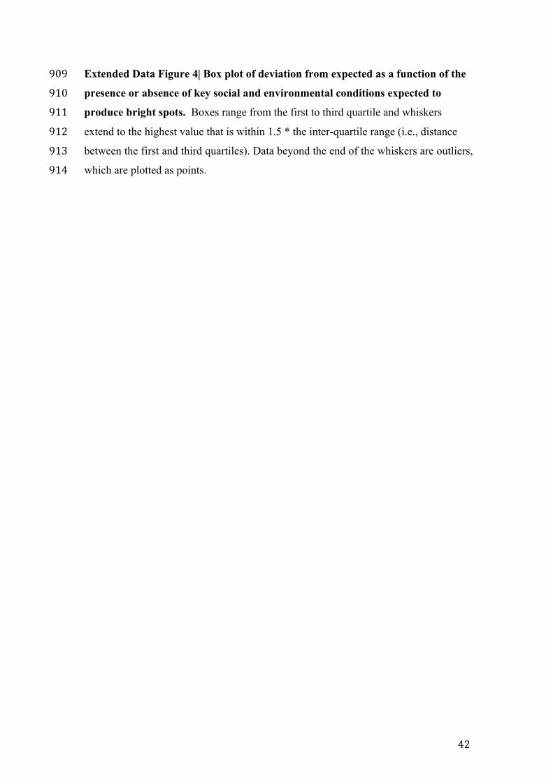
Extended Data Figure 4| Box plot of deviation from expected as a function of the 909
presence or absence of key social and environmental conditions expected to 910
produce bright spots. Boxes range from the first to third quartile and whiskers 911
extend to the highest value that is within 1.5 * the inter-quartile range (i.e., distance 912
between the first and third quartiles). Data beyond the end of the whiskers are outliers, 913
which are plotted as points. 914