access-om: the ocean and sea-ice core ofthe access coupled ... · australian meteorologial and...

Australian Meteorological and Oceanographic Journal 63 (2013) 213–232

213

ACCESS-OM: the ocean and sea-ice core of the ACCESS coupled model

Daohua Bi1, Simon J. Marsland1, Petteri Uotila1, Siobhan O’Farrell1, Russell Fiedler2, Arnold Sullivan1, Stephen M. Griffies3, Xiaobing Zhou4, and Anthony C. Hirst1

1 CAWCR/CSIRO Marine and Atmospheric Research, Aspendale, Australia2 CAWCR/CSIRO Marine and Atmospheric Research, Hobart, Australia

3 NOAA/Geophysical Fluid Dynamics Laboratory, Princeton, NJ, USA4 CAWCR/Bureau of Meteorology, Melbourne, Australia

(Manuscript received July 2012; revised January 2013)

The Australian Community Climate and Earth System Simulator Ocean Model (ACCESS-OM), a global coupled ocean and sea-ice model, has been developed at the Centre for Australian Weather and Climate Research1. It is aimed to serve the Australian climate sciences community, including the Bureau of Meteorology, CSIRO2 and Australian universities, for ocean climate research. ACCESS-OM comprises the NOAA/GFDL3 Modular Ocean Model version 4p1; the LANL4 Sea-ice Model version 4.1, a data atmospheric model; and the CERFACS5 OASIS3.25 coupler, which constrains data exchange between the sub-models. ACCESS-OM has been functioning as the ocean and sea-ice coupling core of the ACCESS cou-pled model, one of the Australian models participating in the Coupled Model In-ter-comparison Project phase 5. This paper describes the ACCESS-OM sub-mod-els, coupler, coupling strategy and framework. A selection of key metrics from an ACCESS-OM benchmark simulation, which has run for 500 years using the Coordinated Ocean-ice Reference Experiments normal year forcing, is presented and compared with observations to evaluate the model performance. It shows ACCESS-OM simulates the global ocean and sea-ice climate generally compara-bly to the results from other ocean sea-ice models of the same class (Griffies et al. 2009). For example, the global ocean volume-averaged temperature undergoes minor evolution. The maximum transport of North Atlantic overturning circula-tion is 18.5 Sv and the Antarctic Circumpolar Current transport through Drake Passage is 150 Sv, both in fair agreement with the observations; and the sea-ice coverage has reasonable distribution and annual cycle. Measured against other ocean sea-ice models and observations, ACCESS-OM is an appropriate tool for Australia’s future ocean climate modelling efforts.

Introduction

This paper documents the Australian Community Climate and Earth System Simulator Ocean Model (ACCESS-OM), once known as the Australian Community Ocean Model (AusCOM; Bi and Marsland 2010). ACCESS-OM has

previously been used for a multi-parameter tuning study of sea-ice (Uotila et al. 2012), and for demonstrating the rapid response of global sea-level rise to both Greenland and Antarctic ice sheet melting events (Lorbacher et al. 2012). ACCESS-OM is developed to serve the Australian climate community with ocean weather and climate research, including seasonal forecasting, climate variability studies, downscaling of climate in the marine environment around Australia, and ocean biogeochemistry modelling. Most importantly, ACCESS-OM is the ocean and sea-ice component of the ACCESS coupled model (ACCESS-CM; Bi et al. 2013), the new generation Australian coupled climate model participating in the Coupled Model Inter-comparison Project phase 5 (CMIP5).

1CAWCR, a partnership between CSIRO and the Bureau of Meteorology.2Commonwealth Industrial Scientific and Industrial Research Organisation.3National Oceanic and Atmospheric Administration/Geophysical Fluid Dynamics Laboratory, Princeton, NJ, USA.4Los Alamos National Laboratory, Los Alamos, NM, USA.5Centre Européen de Recherche et de Formation Avancée en Calcul Scientifique, Toulouse, France

Corresponding author address: Daohua Bi. Email: [email protected]

214 Australian Meteorological and Oceanographic Journal 63:1 March 2013

Building ACCESS-OM has been a key step towards the development of ACCESS-CM in both scientific and technical aspects. ACCESS-OM couples two state-of-the-art models, the NOAA/GFDL ocean model MOM4p1 (Griffies 2009) and the LANL sea-ice model CICE4.1 (Hunke and Lipscomb 2010). A variety of tests and multi-centennial scale simulations in the context of the Coordinated Ocean-ice Reference Experiments (COREs) (Griffies et al. 2009) have been conducted to evaluate the model performance. One of these runs is presented in this study and shows that ACCESS-OM produces a global ocean climate in reasonable agreement with observations and results from other models participating in the COREs. This benchmarking exercise supports the development of a world-class ocean sea-ice component for ACCESS-CM. The ACCESS-OM is built within the OASIS3.25 (Valcke 2006) coupling framework and includes a data model technically mimicking an active atmospheric component communicating with other model components via the coupler. This approach results in a model framework ready for implementing into a fully coupled general circulation model; that is, a significant proportion of the engineering required for the fully coupled ACCESS-CM has been completed in ACCESS-OM.

This paper provides additional detail relevant to that presented on the ocean and sea-ice components in the ACCESS-CM description paper (Bi et al. 2013). It is arranged in the following sections. The model components, coupler, and coupling strategy are described in the section ‘Model description’. The experimental design and the Coordinated Ocean-ice Reference Experiments Normal Year Forcing (CORE NYF) data used for the ACCESS-OM experiments are introduced in the section ‘Experimental design’. Results from a 500-year benchmark run are presented in the section ‘Results’, in comparison with observations and results from other models included in the Griffies et al. (2009) CORE NYF intercomparison paper. The ‘Discussion’ section gives a

discussion on the impact of short-wave penetration on the ocean climate by comparing the benchmark run against a parallel run which uses different short-wave attenuation depth data.

Model description

OceanThe ACCESS-OM ocean component is an implementation of the 2009 public release of the NOAA/GFDL MOM4p1 community code (Griffies 2009). ACCESS-OM is configured as a hydrostatic and Boussinesq (volume conserving) ocean with mass exchange of surface freshwater fluxes. The MOM4p1 code is written with rudimentary general vertical coordinate capabilities employing a quasi-Eulerian algorithm. Readers are referred to Griffies (2009) for a detailed description of the model fundamentals including equations, physics and dynamics; supported coordinates; time stepping schemes; and sub-gridscale parameterisations. A major difference between the ACCESS-OM implementation and the public release of MOM4p1 is the use of the OASIS3.25 coupler to link to the sea-ice model (as described by Bi and Marsland 2010). The ACCESS-OM implementation of OASIS has subsequently been adopted into the forthcoming 2012 public release of MOM4p1. Here, we describe the configuration of MOM4p1 for ACCESS-OM.

The horizontal discretisation of ACCESS-OM uses the Arakawa B-grid (Arakawa and Lamb 1977) with an orthogonal curvilinear grid as shown in Fig. 1. A singularity at the North Pole is avoided by using a tripolar grid following Murray (1996). The northern hemisphere poles in ACCESS-OM are located at 65°N, and at 80°E and 260°E. The southern hemisphere pole is located at 78°S and 0–360°E, enhancing the computational efficiency of the model by ignoring land points over Antarctica. South of 65°N, the resolution of the model is 1° along the zonal direction. In the meridional

Fig.1. ACCESS-OM ocean bathymetry (m) and horizontal grid meshes. Grid lines indicate each fourth row in the orthogonal cur-vilinear ‘zonal’ and ‘meridional’ directions. (a) Northern hemisphere projection showing the tripolar grid over the Arctic. (b) Southern hemisphere projection showing the Mercator meridional grid over the Southern Ocean.

Bi et al.: ACCESS-OM: The ocean and sea-ice core of the ACCESS coupled model 215

direction the grid spacing is nominally 1° resolution, with the following three refinements: a) tripolar Arctic north of 65°N; b) equatorial refinement to 1/3° between 10°S and 10°N; and c) a Mercator (cosine-dependent) implementation for the southern hemisphere, ranging from 0.25° at 78°S to 1° at 30°S. This configuration gives a 360 x 300 logically rectangular horizontal mesh. The sea-ice component is configured onto the same grid for a range of benefits, particularly the convenience of ocean sea-ice communication.

The initial bathymetric dataset was obtained from NOAA/GFDL and was derived from a dataset assembled at the Southampton Oceanography Centre as described in Griffies et al. (2005). In contrast to the GFDL-MOM4 implementation, the ACCESS-OM does not have closed regional seas (e.g. Mediterranean, Hudson Bay, Gulf of Arabia, and Persian Gulf). The bathymetric dataset was extensively modified in the region of the Indonesian Throughflow (Makassar, Halmahera, Lifamatola, Lombok, Ombai, Timor and Vitiaz Straits) to improve Pacific-Indian interactions that are important to Australian climate. To improve representation of the deep water formation in the North Atlantic, Denmark Strait and Faroe Bank Channel were deepened, and the main ridges between Greenland and Scotland shoaled. Modifications were also made to allow an oceanic connection representative of the Northwest Passage through the Canadian Archipelago. At the Antarctic margin at least one grid cell of shelf bathymetry was included. Ice shelf regions in the Amery, Weddell and Ross Sea regions were filled. Islands such as New Zealand and Japan were added.

The ACCESS-OM vertical discretisation uses the z* coordinate6. There are 50 model levels covering 0–6000 metres with a resolution ranging from 10 m in the upper layers (0–200 m) to about 333 m for the abyssal ocean. The shallowest water column depth is set to 40 m. While conventional z (height) coordinate models represent free surface variations by using a variable thickness upper layer, the z* coordinate re-scales the height coordinate and treats the time-dependent free surface as a coordinate surface, i.e. z* ≡ 0 at the free surface (z= η). The finite volume method (for discretising the model) within the z* coordinate framework allows an accurate representation of topography by means of shaped volumes (shaved cells; Adcroft et al. 1997) or variable bottom layer thickness (partial cells; Pacanowski and Gnanadesikan 1998) and has been demonstrated to overcome the inadequacies of height coordinates in representing topography (Adcroft and Campin 2004). Additionally, the z* coordinate also allows for more accurate treatment of sea-ice in the model, by removing the problem of disappearing levels when the sea-ice thickness exceeds the thickness of the upper levels.

Details of the physical schemes and sub-gridscale parameterisations used in ACCESS-OM are given in Table 1.

ACCESS-OM uses an isotropic Laplacian friction operator with a viscosity set by a constant velocity scale of 10 cm/s and the squared horizontal grid-scale. This viscosity is additionally scaled down in regions such as the tropics where the local Rossby radius of deformation is larger than the horizontal grid scale. We also employ a horizontal biharmonic friction operator whose viscosity is enhanced in western boundary regions. The combination of lateral Laplacian plus biharmonic friction operators aims to suppress grid noise inherent in under-dissipated flow simulations, while allowing for strong boundary and equatorial current structures consistent with the model’s grid resolution.

The CSIRO short-wave scheme for ACCESS-OM follows a single exponential decay rule e.g. Morel and Antoine (1994) to calculate ocean absorption of the penetrative solar radiation7, using climatological short-wave attenuation depth (SWAD) data. ACCESS-OM uses the diffuse attenuation coefficient (Kd, SWAD = 1/Kd) of the downwelling photosynthetically-available radiation (KdPAR) from the Sea-viewing Wide Field-of-view Sensor (SeaWiFS) Project dataset (Cracknell et al. 2001). ACCESS-CM (Bi et. al. 2013), however, inadvertently uses Kd490 (the default for the CSIRO SW scheme), which is the diffuse attenuation coefficient of the downwelling spectral irradiance at wavelength 490 nm, for the CMIP5 experiments (Dix et al. 2013, Marsland et al. 2013). The KdPAR data covers a broader, more representative spectrum of light and is considered to be more appropriate for use in the ocean model. We note that, in ACCESS-OM (and also ACCESS-CM) a maximum depth is set to 120 m for the short-wave penetration into ocean. This has essentially no effect on the model solution, as confirmed by ACCESS-OM test runs without such penetration limit.

The ACCESS-OM ocean vertical mixing parameterisation is a combination of three different components: a K profile parameterisation for the surface mixed layer (KPP; Large et al. 1994), a tidal mixing parameterisation for the abyssal ocean (Simmons et al. 2004) and coastal oceans (Lee et al. 2006), and background vertical diffusivity (k) everywhere else which depends only on latitude. Outside the tropics k is set equal to a nominal value k0 (= 1 × 10–5 m2 s–1). Following Jochum (2009), ACCESS-OM sets a tropical band (|φ| ≤ 20°) in which k is smoothly reduced from the nominal value to a minimum (keq) of 0.1 × 10–5 m2 s–1 at the equator8. This approach is based on theory and observations that there are latitudinal bands with distinctly different diffusivities (e.g. see Jochum 2009, and references therein), and improves the simulation of ENSO in the ACCESS-CM.

6z* is a quasi-horizontal rescaled height coordinate of Stacey et al. (1995) and Adcroft and Campin (2004). It defines the vertical coordinate as z* = H(z–η)/(H+η), where H is the ‘reference’ depth of the ocean column, η is the local free surface elevation, z is the height (–H ≤ z ≤ η). The range over which z* varies is time independent –H ≤ z* ≤ 0. Hence, all cells remain non-vanishing, so long as the surface elevation maintains η > -H.

7The incident solar radiation with wavelength between 300 nm and 750 nm. Solar radiation with wavelength above 750 nm is non-penetrative and essentially absorbed in the first layer of the model.8Within the tropical band, the background diffusivity is defined as k = a cosφ + b, where a = (k0 – keq) / (cos φ0 – 1 ), b = keq – a, and φ is latitude, φ0=± 20° is the boundary of the band.


ACCESS-OM does not use sea surface temperature (SST) restoring. However, it uses strong sea surface salinity (SSS) restoring (15 days over the upper layer of nominal 10 m thickness) and employs water fluxes rather than virtual salt fluxes at the upper boundary. It conserves water volume by using global ocean water flux correction. With water and salt conservation enforced in the model ocean, the only source of salt for the ocean is from the small amount of salt exchange between ocean and sea-ice due to ice formation and melting. It should be noted that, when computing the restoring flux for salinity, ACCESS-OM sets a maximum absolute value

(i.e., max_delta_salinity_restore = 0.5 psu) for the difference between model SSS and the restoring SSS. This approach is useful especially in the North Atlantic western boundary, where poor Gulf Stream separation can lead to large salinity biases. Doing so can avoid spurious transport of large amount of fresh water (due to too much SSS restoring) to the North Atlantic subpolar gyre and the resultant impact on the overturning circulation. On the other hand, however, this approach also sets loose the constraints on the SSS in those regions where SSS biases are large due to forcing errors and allows the model SSS to drift away from the restoring SSS.

Table 1. Physical configurations and parameterisations for MOM4p1 in ACCESS-OM.

Item Scheme/choice MOM4p1 Parameters

Time stepping for tracer and baroclinic velocity

Two-level forward step; tracer and velocity are staggered in time; Predictor-Corrector scheme. Baroclinic timestep = 3600 s

dtts = dtuv = 3600 s

Barotropic time stepping Split-explicit time stepping: fast 2D dynamics is sub-cycled within the slower 3D dynamics.

dtbt = 45 s

Coriolis force time stepping Semi-implicit: half the force is evaluated at the present time and half at the future time.

dtime = acor * dtuvacor = 0.5

Measure of ocean thermal state

Conservative temperature (McDougall 2003).

Bottom topography Partial bottom step (Pacanowski and Gnanadesikan 1998) is allowed.

Tracer advection Multi-dimensional flux limited scheme (Sweby 1984, Hunds-dorfer and Trompert 1994), referred to as the Sweby scheme, for all tracers, with fast-compute turned on.

Short-wave radiation penetra-tion

CSIRO scheme, with prescribed SeaWiFs attenuation depth data. Maximum penetration 120 m.

zmax_pen = 120.0 m(see text for details)

Subgrid scale parameterisations

Horizontal friction Smagorinsky iosotropic biharmonic friction after Griffies and Hallberg (2000);Laplacian MICOM isotropic (see text for details).

k_smag_iso = 2.0

vel_micom_iso = 0.10 ms–1

Convection Explicit convection following Rahmstorf (1993)

Vertical mixing KPP scheme of Large et al. (1994).Critical Richardson number 0.3;

Background vertical diffusion is reduced in tropics (see text for details).

ricr = 0.3

background_diffusivity = 1 × 10–5 m2 s–1 background_viscosity = 1 × 10–4 m2 s–1

Neutral physics Isoneutral diffusion (Redi 1982); A modified Gent and McWil-liams (1990) scheme in which skew diffusion relaxes neutral directions toward surfaces of constant generalized vertical coordinate rather than constant geopotential surfaces (Ferrari et al. 2010), with baroclinic closure of the thickness diffusivity.

number_bc_modes = 2bvp_bc_mode = 2bvp_speed = 0.0 m s–1

bvp_min_speed = 0.1 m s –1smax_psi = 0.01epsln_bv_freq = 1 × 10–12 kgm–4

turb_blayer_min = 50.0 m

agm_closure_min = 50.0 m2 s–1

agm_closure_max = 600.0 m2 s–1

Submesoscale Submesoscale mixed layer restratification scheme (Fox-Kem-per et al. 2011)

Tidal mixing Baroclinic abyssal tidal dissipation scheme (Simmons et al. 2004)

Barotropic coastal tidal dissipation scheme (Lee et al. 2006)

roughness_scale = 2 × 104 mshelf_depth_cutoff = 160.0 mmax_wave_diffusivity = 10-2 m2 s–1

max_drag_diffusivity = 10-2 m2 s–1

Overflow Sigma transport scheme of Beckmann and Doescher (1997) as well as the mixdownslope scheme from Griffies (2009).


Sea-iceThe sea-ice component of ACCESS-OM is the LANL Community Ice CodE version 4.1 (CICE4.1; Hunke and Lipscomb 2010). CICE computes internal ice stresses by an elastic-viscous-plastic dynamics scheme (Hunke and Dukowicz 1997); uses an incremental linear remapping for estimating the ice advection; and redistributes the ice between thickness categories through ridging and rafting schemes by assuming an exponential redistribution function. The ice model is divided into five thickness categories, and has four vertical ice layers and one snow layer in each category. The sea-ice salinity profile is prescribed and unchanged in time (see Eqn 56 of Hunke and Lipscomb 2010) and the snow is assumed to be fresh. The time step of the sea-ice model is one hour and the momentum equation is solved by using an iterative scheme within each time step. It is coupled with the ocean model at every time step while the atmospheric forcing is updated every six hours by the data atmospheric model via the OASIS coupler (see the following two sub-sections).

The sea-ice model includes many predefined internal parameters impacting the simulated sea-ice distribution (Uotila et al. 2012). Values of the most important thermodynamic and dynamic parameters used in the ACCESS-OM model experiments are listed in Table 2. The short-wave parameterisation scheme chosen was the default NCAR Community Climate System Model version 3 (CCSM3) scheme, where visible and infrared albedos are prescribed. The wavelength of 700 nm separates the visible and infrared

bands. Additionally, in the CCSM3 radiation scheme, ice and snow albedos on both spectral bands depend on the sea-ice or snow surface temperature and thickness. When ice becomes thinner than 0.1 m (see thickness criteria ahmax in Table 2), the ice albedo decreases smoothly, following the arctangent function, toward the open ocean value of 0.06. When the surface temperature rises from –dT_mlt to 0 °C, then the albedo decreases by dalb_mlt. The visible snow albedo decreases by 0.1 and the infrared snow albedo decreases by 0.15 when the snow surface temperature rises from –dT_mlt to 0 °C. The snow patchiness parameter, snowpatch, impacts on how the albedo is averaged over a grid cell weighted by the ratio of ice and snow covered portions as shown by Uotila et al. (2012). Essentially a higher snowpatch value decreases the average albedo. In addition to the variables related to the short-wave radiation scheme, the value of the surface roughness of sea-ice affects the ice-atmosphere momentum and energy exchange and is a predefined constant in the model (see Table 2).

The ice-ocean energy and momentum exchange includes predefined variables, such as the ice-ocean stress drag coefficient, stress turning angle and heat exchange coefficient. Additionally, the minimum value of the ice-ocean friction velocity is predefined. The sensitivity of the sea-ice distribution to the parameters related to the ocean-ice heat exchange has been shown to be comparable or higher than its sensitivity to the parameters used to adjust the short-wave radiation scheme (Hunke 2010, Uotila et al. 2012). In terms of internal ice properties, the ice conductivity needs to

Table 2. Values of selected important dynamic and thermodynamic sea ice model parameters used in the ACCESS-OM model experiments.

short name Value Full name

shortwave Default CCSM3 short-wave radiation scheme

albicev 0.86 Visible ice albedo

albicei 0.44 Infrared ice albedo

albsnowv 0.98 Visible snow albedo

albsnowi 0.70 Infrared snow albedo

snowpatch 0.01 Snow patchiness parameter

dT_mlt 1.0 ˚C Change in temperature in ice to give dalb_mlt albedo change

dalb_mlt –0.02 Albedo change per dT_mlt change

ahmax 0.1 m Albedo is constant above this thickness

nilyr 4 Number of vertical layers in ice

cosw, sinw 0˚ Ocean-ice turning angle

mu_rdg 2 m1/2 e-folding scale of ridged ice

maxraft 1.0 m Maximum thickness of ice that rafts

dragio 0.00536 Ice-ocean drag

ustar_min 0.0005 m s–1 Minimum ice-ocean friction velocity

conduct Bubbly (Pringle et al. 2007) Ice conductivity (temperature-salinity-dependent)

iceruf 0.0005 m Surface roughness of ice

chio 0.004 Ice-ocean heat exchange coefficient

ice_ref_salinity 4 psu Ice reference salinity (used to compute ice-ocean salt fluxes)


be selected as well as the number of vertical layers in ice. The sea-ice deformation is affected by the values of the e-folding scale of ridged ice and the maximum thickness of rafted ice. This ridging parameter affects the sea-ice distribution to the same extent as the albedo values (Uotila et al. 2012). Values of these variables as used in the ACCESS-OM experiments presented in this paper are listed in Table 2.

AtmosphereACCESS-OM uses a data atmospheric model (named as MATM). It is designed at CAWCR to handle various atmospheric forcing data for the coupled ocean and sea-ice model. It is equipped with a set of modules used for reading different datasets (e.g. NCEP2, ERA40, CORE and UM AMIP9 outputs etc.) which may be of different spatial and temporal resolutions and often use different variable names for the same fields. In conjunction with an external ‘fields_table’ and a data file selecting script (both are pre-processed for a specific dataset), this data model reads in the required atmospheric fields, with proper scaling and offsetting treatment wherever needed, and passes them into the coupler. During the simulation the MATM also receives coupling data from the underlying sea-ice model, technically mimicking an active atmospheric model.

CouplerACCESS-OM uses the CERFACS OASIS3.25 (Valcke 2006) numerical coupler. OASIS3.25 is developed under the concepts of portability and flexibility. It runs as a separate mono-process executable, receiving, interpolating when needed, and sending coupling fields between the sub-models which also run as separate executables at the same time. OASIS3.25 links the individual sub-models via a few specific PRISM10 Model Interface Library calls implemented in the sub-models, controlling model synchronisation and data passing (i.e. coupling) via Message Passing Interface (MPI) functions. All interpolations conducted by OASIS3.25 for the ACCESS-OM coupling are performed by the Spherical Coordinate Remapping and Interpolation Package (SCRIPP; Jones 1997). Since ACCESS-OM configures the ocean and sea-ice on the same horizontal Arakawa B-grid (Arakawa and Lamb 1977), fields are exchanged directly with no need of transformation (vector rotation, grid remapping interpolation), which enhances the model’s computational efficiency.

Coupling strategyWithin the ACCESS-OM coupling framework, the sea-ice model is placed between the atmospheric model and ocean model, working as a coupling media and being the only sub-model that needs to communicate with the other two sub-

models simultaneously. The strategy, shown in Fig. 2, is that coupling occurs only between atmosphere and sea-ice, and between sea-ice and ocean, with no direct communication between the atmosphere and ocean models. There are a total of 31 coupling fields in the ACCESS-OM system (ten from atmosphere to ice; 13 from ice to ocean; seven from ocean to ice; and one from ice to atmosphere; see Bi and Marsland (2010) for details. The ocean sea-ice coupling is identical to that for ACCESS-CM. All coupling fields from the source model (atmosphere/ocean) must be gathered, processed jointly with the associated coupling fields from sea-ice itself (the ‘coupling media’) as required, and then delivered to the target model (ocean/atmosphere). This design allows for easy control over the coupling frequencies, with ACCESS-OM using different frequencies for coupling atmosphere to sea-ice (six hours, as determined by the highest temporal resolution of the atmospheric forcing data in the experiments discussed below) and sea-ice to ocean (i.e. at the model time step of one hour).

Experimental design

Atmospheric forcingThe ACCESS-OM has undergone numerous tests with a variety of physical configurations under the CORE Normal Year Forcing (NYF) in the context of CORE-NYF protocols (Griffies et al. 2009). The CORE atmospheric forcing dataset has been developed at NCAR and documented by Large and Yeager (2004, 2009). The CORE-NYF is a composite of NCEP/NCAR reanalysis data, bias-corrected reanalysis data, and observational data. It provides a climatological mean year forcing that incorporates realistic and self-consistent six-hourly variability for air temperature, zonal and meridional wind speeds, specific humidity, and sea level pressure. The radiative heat fluxes (downward long-wave and short-wave fluxes) have daily temporal resolution. The water fluxes include precipitative fluxes (rainfall and snowfall, with daily variability) and river runoff (annual mean climatology).

In this study, the ACCESS-OM 500-year benchmarking run, named as CNYF2-BM, uses the most recent COREv2-NYF data (see e.g. http://data1.gfdl.noaa.gov/nomads/forms/mom4/COREv2.html).

9Atmospheric Model Intercomparison Project, a standard experimental protocol for global atmospheric general circulation models (AGCMs). It provides a community-based infrastructure in support of climate model diagnosis, evaluation, intercomparison, documentation and data access. 10Project for Integrated Earth System Modelling, an infrastructure project for climate research in Europe, funded by the European Commission.

Fig 2. Coupling strategy for the ACCESS-OM (and ACCESS-CM) system.


SetupAs in ACCESS-CM (Bi et al. 2013), ACCESS-OM uses the World Ocean Atlas 2005 (WOA2005) annual mean climatology of temperature (Locarnini et al. 2006) and salinity (Antonov et al. 2006) as the ocean initial condition. The sea-ice is initialised using the WOA2005 January SST and SSS, with grid points that have SST below freezing point and the majority of the area covered with ice of three-metre thickness category.

To assess the impact of different short-wave attenuation data on the model ocean climate, another run (named as CNYF2-SM) is conducted. CNYF2-SM uses Kd490 (as in the ACCESS-CM CMIP5 experiments) and would otherwise be identical to CNYF2-BM. Comparison between CNYF2-SM and CNYF2-BM will be given in the ‘Discussion’ section.

ResultsThis section presents a selection of ocean and sea-ice fields from the CNYF2-BM run. They are compared with observations and results from other models (Griffies et al. 2009, hereafter referred to as Griffies09) for evaluating the skill of ACCESS-OM in simulating the world ocean and sea-ice climate. As in Griffies09, the average of the last ten years of the 500-year integrations is used to represent the model ocean climate. Unless specified, the observational data used for the model to compare against is the World Ocean Atlas 2009 (WOA2009) potential temperature (Locarnini et al. 2010) and salinity (Antonov et al. 2010). Where applicable the model evolution, climate and biases (model minus observation) are shown with the same contour interval and colour scales as used by Griffies09. This choice allows the reader to directly compare the ACCESS-OM results under CORE NYF to those from a group of seven ocean and sea-ice models (hereafter referred to as CORE models), particularly the GFDL-MOM4 (version 4p0) simulation based on similar ocean code and physical configurations, as well as the NCAR-POP simulation that uses the same sea-ice code. Note the primary difference between the GFDL-MOM4 system and ACCESS-OM is that they use different sea-ice codes. Another major difference is that ACCESS-OM uses a horizontal resolution of 360 × 300, in contrast to the 360 × 200 resolution for GFDL-MOM4.

Globally averaged ocean temperature and salinityFigure 3(a) shows the time series of volume-weighted annual mean global ocean potential temperature, revealing the evolution of the ocean heat content. The global ocean warms up slightly in the first two centuries, achieving a maximum warming of 0.13 °C at around year 180, and gradually cools down thereafter. By the end of the integration, the model ocean as a whole comes back to a state very close to the initial thermal condition. This temperature evolution is very mild compared to that of most other CORE models shown in Fig. 3 of Griffies09. As shown below, the overall mild global ocean thermal evolution is the joint effect of complicated changes at different depths in the ocean interior.

Figure 3(b) displays the time series of global average annual mean ocean salinity. A very weak freshening trend is observed through the 500-year integration, with the final salinity decrease less than 0.002 psu. Note that ACCESS-OM uses a strong surface salinity restoring (15 days over the upper layer of nominal 10 m thickness) and employs water fluxes at the upper boundary. With water and salt conservation enforced in the model ocean, the only source of salt for the ocean is from the small amount of salt exchange between ocean and sea-ice due to ice formation and melting. Therefore the potential drift of ocean salt content is suppressed, and the model achieves a quasi-stationary evolution of the global mean salinity.

Nevertheless, the minor changes in the evolution of temperature and quasi-stability of salinity places ACCESS-OM among the better CORE models that show reasonable thermal and salt closure in the global ocean (see Griffies09).

Horizontally averaged global ocean temperature and salinityFigure 4(a) presents evolutions of the horizontally averaged annual mean potential temperature errors, revealing the depth-dependent thermal adjustment. While the upper layer (0-80 m) water sees slight but persistent cooling errors (< 0.1 ˚C), the subsurface to mid-depth ocean (100–1600 m) undergoes significant warming which develops rapidly in the first two centuries and generally stabilises thereafter. This warming is centered within the 600–800 m

Fig. 3. Simulated evolution of the annual mean, volume-weighted global ocean (a) potential temperature (°C) and (b) salinity (psu).


depth range and the maximum error is about 1.1 ˚C. Such a thermal adjustment (cooling near the surface and warming underneath) is similar to that seen in the GFDL MOM model CORE NYF run shown in Fig. 5 of Griffies09. This is due to ACCESS-OM and GFDL MOM using similar ocean code and parameterisation choices. However, in the deep ocean below 2000 m, ACCESS-OM shows gradual and steady cooling in the course of the CNYF2-BM run, in contrast to the GFDL MOM run which sees very slight warming in the deep ocean. Similar cooling drifts in abyssal ocean are also seen in some other CORE models such as the NCAR POP, Kiel Orca and MPI models shown by Griffies09.

Figure 4(b) shows the time series of horizontally averaged annual mean salinity errors in the CNYF2-BM simulation. Like temperature, salinity is evolving at all depths towards a solution that has evident positive biases at the mid-depth and negative biases in the abyssal ocean, with the maximum salinity increase of about 0.16 psu at around 600 m and the maximum freshening error of 0.08 psu near the ocean bottom. Again, such a depth-dependent evolution of salinity is not uncommon in the CORE models. Unsurprisingly, the GFDL MOM model shows trends and magnitude of salinity drifts in the ocean interior very similar to the ACCESS-OM result (see Fig. 6 in Griffies09) .

Zonal mean temperature and salinityFigure 5 shows the observed zonal average potential temperature and salinity, and the ACCESS-OM bias represented by the CNYF2-BM climate minus observation (Locarnini et al. 2010, Antonov et al. 2010). It is seen from Figs. 5(c) and 5(d) that ACCESS-OM is generally too warm and saline in the subsurface and intermediate waters north of 50˚S. The most evident errors are found in the Southern Ocean where the Antarctic Intermediate Water (AAIW) is poorly represented, with maximum warm and saline biases (located around 40˚S, 600 m) being over 2.0 ˚C and 0.4 psu, respectively. Due to the large and extensive saline error

(which is possibly the joint effect of too little subduction and incorrect isopycnal mixing rate), the northward penetrating fresh tongue of AAIW is largely weakened. Note the AAIW salt biases in the Atlantic sector (not shown) are larger than that of the global zonal mean shown in Fig. 5(d). While a majority of the water property biases are confined between 45˚S and 45˚N and within the 400–1000 m layer, noticeable deep, warm and saline errors are found in the 60˚–80˚N band (North Atlantic sector), due to local spurious deep convective mixing and overturning (see the ‘Mixed layer depth’ subsection). The high latitude Southern Ocean (south of 60˚S) sees deep cooling and freshening biases, indicating the model deficiency in simulating the Antarctic Bottom Water (AABW) properties. Furthermore, via the transport of deep ocean meridional overturning circulation (MOC) (see Fig. 9), the biased AABW spreads northward, bringing the cold and fresh biases into the global deep and abyssal ocean (below 2000 m). Despite the above notable biases, the ACCESS-OM simulation shows drifts in the zonal mean temperature and salinity within ±2.0 ˚C and ±0.4 psu, respectively, over most regions, generally comparable to the best results from the CORE models shown in Griffies09.

Surface water propertiesFigure 6(a) shows the ACCESS-OM SST bias map derived from the CNYF2-BM climate minus the observation (Locarnini et al. 2010). The large-scale thermal error pattern is very similar to that from some of the other CORE models, especially the GFDL MOM, as shown in Fig. 7 of Griffies09. Some of the common errors found in other CORE models also appear in the ACCESS-OM simulation, including the large warm biases along major frontal zones such as the North Pacific and North Atlantic western boundary currents (i.e. Kuroshio Current and Gulf Stream). The non-eddy permitting resolution of these models means that they are unable to represent the frontal current structure and position properly. As is well known, ocean frontal zones

Fig. 4. Evolution of horizontally averaged annual mean global ocean anomalies of potential temperature (left, °C) and salinity (right, psu). The 0–1600 m layer has been stretched and 0.5 °C contours for ΔT and 0.05 psu contours for ΔS are drawn to better gauge the drift. The anomalies are defined as model – observation (WOA 2009) (Locarnini et al. 2010, Antonov et al. 2010).


have strong SST gradients, and any shift of the location and biases of intensity of the simulated frontal flows results in large SST biases. The strong cooling error located southeast of the Labrador Sea occurs for similar reasons.

In other regions of the world ocean, ACCESS-OM shows moderate or trivial thermal biases compared to other CORE models. For example, the tropical Pacific cold bias evident in five out of the seven CORE models including GFDL MOM is considerably smaller in CNYF2-BM, probably owing to the reduction of background vertical diffusivity in the equatorial

oceans suppressing the vertical mixing (see the ‘Model description’ section). This vertical mixing modification improves the model performance and results in better ENSO simulation in the ACCESS-CM CMIP5 experiments. In addition, while all other CORE models show warm biases near the west coasts of the American and African continents, the ACCESS-OM run CNYF2-BM shows relatively mild errors in these coastal regions. One of the reasons for this warm bias may be deficient wind stress forcing associated with coarse resolutions of both the model and the forcing

Fig. 5. Global ocean zonal mean temperature (left, °C) and salinity (right, psu). (a) observation; (b) model errors, defined as CNYF2-BM last 10-year average – Observation (WOA2009).

Fig. 6. The CNYF2-BM run sea surface temperature and salinity biases (model – WOA2009 observation). Units: °C for temperature (a) and psu for salinity (b).


data that fail to represent correct paths and intensities of the equator-ward winds along the model coasts. For instance, weak (equatorward) winds result in weak (westward) Ekman drift at the surface and therefore less upwelling off the coasts. Consequently, less cold water is brought up to the surface from underneath, causing warm SST biases over the coastal regions.

Figure 6(b) presents the ACCESS-OM SSS bias relative to observation (Antonov et al. 2010). In general, SSS biases are

small over the majority of the world ocean. This is achieved since CNYF2-BM uses strong SSS relaxation (10 m/15 days) which holds the model SSS close to the restoring SSS over regions where the SSS tendencies are relatively small. Thus over the majority of the world ocean the SSS biases are within ±0.5 psu (the preset maximum absolute difference between the model SSS and restoring SSS).

Large SSS biases appear in the Arctic Ocean due to a number of reasons, including poor river runoff data, possible

Fig. 7. Tropical Pacific thermocline ((a) and (b); °C) and upper ocean zonal velocity component ((c) and (d); m s–1). Left panels are from observations (Johnson et al. 2002) and right panels are from CNYF2-BM.

Fig. 8. Annual maximum mixed layer depth of: (a) observed estimate, and (b) CNYF2-BM. Units: m. The model result is the last 10-year mean of the maximum MLD in each annual cycle, and the observed estimated is diagnosed from long-term month-ly temperature salinity climatology, as detailed in Griffies09.


deficiency in observations, and the preset limit for the SSS restoring allowing for literally free drift of SSS. Hudson Bay also sees large positive SSS error, primarily owing to the significant difference there between the WOA2009 SSS data (used for bias calculation) and WOA2005 SSS data (the restoring data). In the North Atlantic Ocean, there is a noticeable saline bias within the Gulf Stream and a fresh bias southeast of the Labrador Sea, in a similar location to the SST biases shown in Fig. 6(a). These biases are the result of the model deficiency in resolving the Gulf Stream path, and the 0.5 psu limit set for the SSS restoring mentioned above.

Tropical Pacific features Equatorial processes are important for understanding the influence of the ocean on the atmosphere, and the tropical Pacific is one of the key regions that impact on the global climate system. Specifically, the equatorial Pacific Ocean currents play a critical role in modulating the atmosphere-ocean interactions, especially through the El Niño–Southern Oscillation and associated processes, and global climatic teleconnections. For all coupled atmosphere-ocean models, realistic simulation of the tropical Pacific behaviour and therefore ENSO activities is one of the most important and challenging goals. To achieve this goal, it is essential for the ocean models be able to represent realistic tropical Pacific thermodynamic and dynamic features under prescribed, realistic atmospheric forcing.

Figures 7(a) and 7(c) show the vertical distributions of annual mean temperature in the upper equatorial Pacific Ocean from observations (Johnson et al. 2002) and the ACCESS-OM simulation, respectively. The observations are characterised by a permanent, thin layer of warm water over deeper, colder water. The mixed layer is deep in the western warm pool region and very shallow in the east. ACCESS-OM shows a fairly close match to the observation in terms of the thermocline structure, penetration depth of the western warm pool and the eastern shoaling of the thermocline. However, as commonly seen in the other CORE models, some biases are noticeable in the CNYF2-BM result. For example, the centre of the western warm pool is shifted east. It is also somewhat warmer and penetrates deeper in the central Pacific, resulting in steeper shoaling of the thermocline between 170°W–120°W than shown in the observations (Fig. 7(a)).

Figure 7(b) and 7(d) present the observations of the vertical structure of the upper layer zonal velocity in the equatorial Pacific Ocean (Johnson et al. 2002) and the same result for the CNYF2-BM simulation. The model result agrees fairly well with the observations, particularly in terms of the location of the maximum flow (140°W–120°W, around the 100 m depth) and intensity (over 1 m s–1) of the undercurrent centre. Observations show that the wind-driven westward surface currents are confined by the strong vertical stratification in the mixed layer and upper thermocline, which is mirrored in the ACCESS-OM simulations. However, there are some evident biases in the model result. The simulated

undercurrent shows a vertical structure that is too weak in the west and too strong in the east because of the gradient in the thermal stratification. The near surface westward flow is too weak in the west and too strong in the east, possibly due to errors in the westward wind stress forcing. Despite not being strong enough towards the eastern boundary of the ocean, the ACCESS-OM simulated equatorial undercurrent does not show the same error in the extension to the eastern Pacific seen in some of the other CORE models (see Fig. 14 of Griffies09). In fact, ACCESS-OM has quite a strong current (~0.4 m s–1) at 90°W in the CNYF2-BM simulation.

Mixed layer depth The ocean mixed layer is the oceanic surface zone that responds directly and rapidly to atmospheric forcing, and through it atmosphere and ocean influence each other. Processes determining the mixed layer depth (MLD) include wind-driven mixing, subduction, atmosphere-ocean heat and fresh water exchanges, and gravitation-induced convective overturning. Maximum MLD attained during an annual cycle is an important index reflecting the depth of rapid overturn of surface water (occurring in later winter) which is closely related to the ocean water mass formations.

The observed estimate of the maximum MLD (Griffies09) and the annual maximum MLD averaged over the last ten years of CNYF2-BM is presented in Fig. 8. ACCESS-OM simulates reasonably the winter deep mixed layer in the subpolar North Atlantic Ocean (which is associated with the North Atlantic deep water (NADW) formation) in terms of depth, extent and location. It also represents the band of deeper mixed layers extending along the northern flank of the Antarctic Circumpolar Current (ACC) in the Indian and Pacific Oceans. This band of deeper mixed layers is associated with the Sub-Antarctic Mode Water (SAMW). It generally has a penetration depth down to 300–700 m in the observation (Fig. 8(a)) but 200–500 m in the CNYF2-BM simulation (Fig. 8(b)). In the high latitude Southern Ocean, ACCESS-OM simulates spuriously extensive and deep mixed layers in the Weddell Sea. In fact, the CNYF2-BM run yields persistent deep winter convection down to the bottom in the Weddell Sea, in contrast to observations which show convection generally shallower then 1000 m with only occasionally deep convection down to 4000 m. This model feature has implications for the rate of the Antarctic Bottom Water (AABW) formation which in the model is determined by the convective overturning off Antarctica. In addition, the spuriously deep convection increases the oceanic heat flux, which melts the sea-ice and contributes to the negative biases of sea-ice thickness shown in the Weddell Sea (Fig. 13(d)). It also potentially causes the sea-ice drift to be more wind dependent (Fig. 15(d)) due to the reduced sea-ice concentration and thickness, since thinner ice deviates less from the wind direction than thicker ice.


Meridional overturning circulations The Atlantic and global ocean MOC stream functions of the CNYF2-BM last 10-year mean are shown in Figs. 9(a) and 9(b), respectively. The main features of the global ocean MOC (GMOC) are the vigorous tropical wind-driven cells which are strong and shallow, the Deacon Cell driven by the southern hemisphere sub-polar westerlies, the Antarctic Bottom Water (AABW) cell south of 60°S, the Southern Ocean abyssal cell (here referred to as SOAC), and the North Atlantic deep water (NADW) cell.

Figures 9(c) and 9(d) show the time series of MOC indices from the CNYF2-BM simulation. The AABW and SOAC transport indices undergo a rapid decline in the first few decades and then gradually recover towards quasi-stability. The NADW and AMOC26N transports also show a rapid initial decline and slow recovery, and then start developing into regular quasi-decadal oscillations from around year 350 onwards. These oscillations are a sign of mixed-boundary condition variability associated with the features of the normal year forcing, which has been discussed in detail by Griffies09 (see Fig. 26 therein). By the end of the 500-year

integration, ACCESS-OM is in quasi-equilibrium with the NADW intensity being about 18.5 Sv. This result is somewhat stronger than the value of ~15 Sv from observations (e.g. Ganachaud 2003, Lumpkin et al. 2008, Ganachaud and Wunsch 2000), and significantly larger than the results from all other CORE models (<13.5 Sv) except GFDL MOM which represents the highest AMOC transport of about 20 Sv (see Fig. 25 of Griffies09). The AMOC26N ends up being about 15.5 Sv, which is within the range of 10–25 Sv from the RAPID-WATCH observation of AMOC transport at 26°N over the period of 2004–2008 (Hermanson et al. 2010).

In the Southern Ocean, the AABW cell evolves with no evident variability or oscillation and has a maximum transport of about 5.5 Sv by the end of the run. This rate is comparable to other CORE results that range from 5 to 10 Sv, but small compared to observations (e.g. Naveira Garabato et al. (2002) report a diagnosed AABW formation of 9.77 ± 3.7 Sv in the Weddell Sea). Despite the relatively weak AABW cell, the SOAC circulation is very active in ACCESS-OM. The maximum transport evolves with noticeable quasi-decadal variability in the second half of the simulations and

Fig. 9. Simulated MOC patterns and evolutions of some major transport indices: (a) Atlantic MOC, (b) global MOC, (c) NADW and AMOC26N indices, and (d) AABW and Southern Ocean abyssal cell (referred to as SOAC) indices. NADW index in defined as the maximum transport of AMOC (at 40°N); AMOC26N index is the maximum AMOC transport at 26°N; AABW index is the maximum transport of global MOC adjacent to Antarctica (south to 60°S); and SOAC index is the maximum transport of the global MOC Southern Ocean abyssal cell (60°S–20°S, below 3000 m). Units: Sv (106 m3 s–1).


settles at around 14 Sv, comparable to the results from other CORE models which range from 6 to 20 Sv. This abyssal cell transports the newly formed cold and fresh AABW northward to high north latitudes in all ocean basins. In the North Atlantic Ocean, this intruding cold, dense water penetrates underneath (and pushes up) the warm, less dense NADW. This is the reason that the modelled AMOC cell penetrates down only to about 3000 m depth, as shown in Fig. 9(a). Consequently, the whole abyssal ocean is gradually filled with cold and fresh water (see Figs 4 and 6), and the global ocean as a whole is slowly cooling, as shown in Fig. 3(a).

Barotropic flow and ACC transportThe barotropic streamfunction depicts the vertically integrated horizontal water volume transport by the major currents and gyres of the global ocean. The map of the simulated barotropic flows of the CNYF2-BM run is shown in Fig. 10(a). All the major horizontal circulations are well captured, including the Antarctic Circumpolar Current (ACC), the anti-cyclonic subtropical gyres in the Indian, Pacific and Atlantic Oceans, and the cyclonic tropical gyres.

While the cyclonic subpolar gyre in the North Atlantic is strong, its counterpart in the North Pacific is very weak. The western boundary currents, i.e. the poleward branches of the subtropical gyres, are all strong. These features are primarily determined by the wind forcing and have climatic consequence. For example, the strong Kuroshio Current has a maximum transport rate of over 40 Sv, bringing warm and salty surface water too far north and causing the spuriously large warm and saline biases northeast of Japan (see Fig. 6(a)). This occurs possibly because the North Pacific subpolar gyre is too weak to counter the intrusion of the stronger Kuroshio Current. However, the situation for the North Atlantic Ocean is the opposite. The simulated Gulf Stream has a maximum transport rate of over 30 Sv, which is in reasonable agreement with the observed estimate (~35 Sv at 26°N) from RAPID-WATCH (Hermanson et al. 2010). This strong flow, carrying warm and saline water from the

tropics, is forced to turn east before reaching high latitudes by the strong subpolar gyre south of Greenland, resulting in the large cool and fresh biases there, as shown in Figs 6(a) and 6(b).

Figure 10(b) presents the time series of annual mean ACC transport through Drake Passage (referred to as ACC transport) simulated in CNYF2-BM. The ACC transport decreases in the first 100 years and gradually recovers and stabilises at a level of about 150 Sv. This value is slightly above the observed estimates of 134 ± 13 Sv (Whitworth and Peterson 1985), but comparable to the results from the other CORE models, which range from 80 to 180 Sv, as shown by Griffies09 (see Fig. 10 therein).

Sea-ice performance

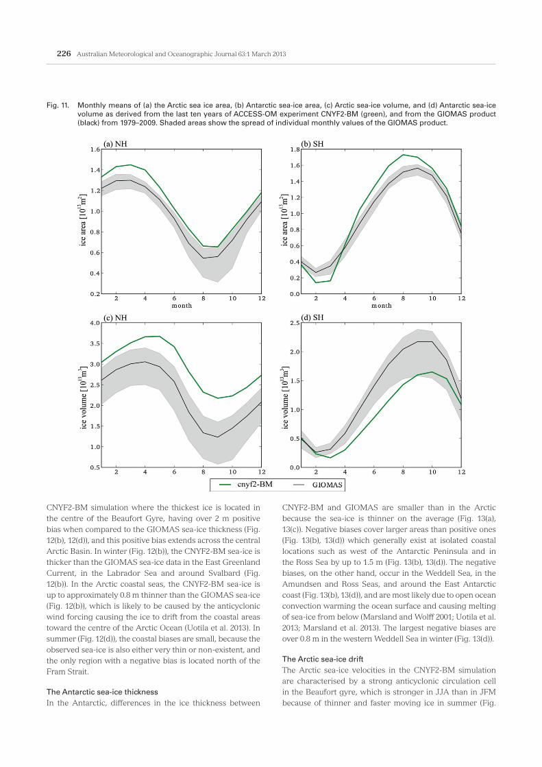
The sea-ice area and volume The CNYF2-BM simulation has a positive sea-ice area bias, except in the Antarctic from January to April (Fig. 11(a), 11(b)). In terms of the sea-ice volume, ACCESS-OM shows higher values in the Arctic than the GIOMAS product (Lindsay and Zhang 2006, Schweiger et al. 2011; Fig. 11(c)), while in the Antarctic its sea-ice volume is lower than GIOMAS in every month except in January (Fig. 11(d)). As discussed by Uotila et al. (2012), the normal year atmospheric forcing results in small amounts of ice leaving the Arctic Ocean through Fram Strait and the ice is accumulated in the Beaufort Gyre instead.

In the Antarctic, the seasonal amplitude of sea-ice area in the ACCESS-OM simulation is larger than that of GIOMAS, and although sea-ice extends over large areas, it remains rather thin (Fig. 11(b), 11(d)).

The Arctic sea-ice thicknessAccording to the observations (e.g. Kwok and Rothrock 2009) and the GIOMAS product, the thickest Arctic ice of over 4 m is found in the Nansen Basin north of Greenland (Fig. 12(a), 12(c)). This is not the case in the ACCESS-OM

Fig. 10. (a) CNYF2-BM last 10-year mean global ocean barotropic streamfunction, and (b) evolution of the ACC transport through Drake Passage. Units: Sv.


CNYF2-BM simulation where the thickest ice is located in the centre of the Beaufort Gyre, having over 2 m positive bias when compared to the GIOMAS sea-ice thickness (Fig. 12(b), 12(d)), and this positive bias extends across the central Arctic Basin. In winter (Fig. 12(b)), the CNYF2-BM sea-ice is thicker than the GIOMAS sea-ice data in the East Greenland Current, in the Labrador Sea and around Svalbard (Fig. 12(b)). In the Arctic coastal seas, the CNYF2-BM sea-ice is up to approximately 0.8 m thinner than the GIOMAS sea-ice (Fig. 12(b)), which is likely to be caused by the anticyclonic wind forcing causing the ice to drift from the coastal areas toward the centre of the Arctic Ocean (Uotila et al. 2013). In summer (Fig. 12(d)), the coastal biases are small, because the observed sea-ice is also either very thin or non-existent, and the only region with a negative bias is located north of the Fram Strait.

The Antarctic sea-ice thicknessIn the Antarctic, differences in the ice thickness between

CNYF2-BM and GIOMAS are smaller than in the Arctic because the sea-ice is thinner on the average (Fig. 13(a), 13(c)). Negative biases cover larger areas than positive ones (Fig. 13(b), 13(d)) which generally exist at isolated coastal locations such as west of the Antarctic Peninsula and in the Ross Sea by up to 1.5 m (Fig. 13(b), 13(d)). The negative biases, on the other hand, occur in the Weddell Sea, in the Amundsen and Ross Seas, and around the East Antarctic coast (Fig. 13(b), 13(d)), and are most likely due to open ocean convection warming the ocean surface and causing melting of sea-ice from below (Marsland and Wolff 2001; Uotila et al. 2013; Marsland et al. 2013). The largest negative biases are over 0.8 m in the western Weddell Sea in winter (Fig. 13(d)).

The Arctic sea-ice driftThe Arctic sea-ice velocities in the CNYF2-BM simulation are characterised by a strong anticyclonic circulation cell in the Beaufort gyre, which is stronger in JJA than in JFM because of thinner and faster moving ice in summer (Fig.

Fig. 11. Monthly means of (a) the Arctic sea ice area, (b) Antarctic sea-ice area, (c) Arctic sea-ice volume, and (d) Antarctic sea-ice volume as derived from the last ten years of ACCESS-OM experiment CNYF2-BM (green), and from the GIOMAS product (black) from 1979–2009. Shaded areas show the spread of individual monthly values of the GIOMAS product.


Fig. 12. The Arctic (a) GIOMAS mean ice thickness from 1979–2009 and (b) the difference between CNYF2-BM and GIOMAS in JFM, and (c) GIOMAS ice thickness and (d) the difference between CNYF2-BM and GIOMAS in JJA. The CNYF2-BM sea-ice thick-ness is derived from the last 30 years of the simulation.

Fig. 13. As Fig. 12 but for the Antarctic.


14(b), 14(d)). The GIOMAS sea-ice velocities also show an anticyclonic circulation cell in the western Arctic, but it is much weaker and smaller than in the ACCESS-OM simulation. As discussed earlier, the strong anticyclonic circulation in CNYF2-BM is directly related to the normal year atmospheric forcing and results in positive sea-ice thickness and concentration biases in the central Arctic. Another prominent feature in the JJA CNYF2-BM mean sea-ice velocity field is the strong sea-ice drift out of the east Arctic Ocean to the East Greenland Current via Fram Strait and from the Labrador Sea to the North Atlantic. The sea-ice drift through the Bering Strait is very different in CNYF2-BM compared to GIOMAS. In JFM (JJA), the CNYF2-BM sea-ice motion is southward (northward), while in GIOMAS it is to the north (south). This difference may reflect how differently the models resolve the narrow Bering Strait and could also indicate how the water and heat fluxes are resolved in ACCESS-OM (see also Uotila et al. 2013).

The Antarctic sea-ice driftIn the Antarctic, the CNYF2-BM sea-ice drift appears more meandering than the GIOMAS sea-ice drift (Fig. 15). The sea-ice in GIOMAS tends to move northeastward towards the ACC and then melt, while in CNYF2-BM the sea-ice drifts eastward under the westerly winds of the Antarctic Circumpolar Trough. Both models have a similar representation of the East Wind Drift along the Antarctic coast. The ACCESS-OM simulation shows several distinctive cyclonic circulation cells in the Weddell Sea, in the Amundsen Sea, along East Antarctica between 90°E and 150°E, and between 0°E and 30°E which are almost missing or weak in the GIOMAS sea-ice velocity fields. As in the Arctic, it is possible that these circulation cells are results of the normal year atmospheric forcing, because they are either missing or much less distinctive in the ACCESS-CM CMIP5 simulations (Uotila et al. 2013).

Discussion: impact of short-wave attenuation depth datasets on the ocean climate simulation

As stated earlier, ACCESS-CM inadvertently uses the Kd490

data for calculating short-wave absorption in the ocean. This choice will alter the thermocline temperatures and there will be compensating changes to the salinity and dynamics in the ocean which will feed through back to the coupled system with potential to alter climate modes (e.g. ENSO). Because of the low computational efficiency of the fully coupled model, it is impractical to run ACCESS-CM itself for multi-hundred years to address how the model will respond in a long climate simulation. Therefore, we use an ACCESS-OM simulation for an analogous test run even though the feedbacks to the atmosphere seen in the coupled system cannot be included. The ACCESS-OM 500-year run, using Kd490, CNYF2-SW, is presented here and compared against CNYF2-BM to assess the impact of different SW attenuation

depth data on the world ocean climate simulation. Figure 16(a) shows the pattern of SeaWiFS SW attenuation

depth SWADPAR (i.e. 1/KdPAR) used in CNYF2-BM and Fig. 16(b) shows the annual mean difference between SWAD490 (i.e. 1/ Kd490) and SWADPAR. SWAD490 is significantly deeper than SWADPAR almost everywhere, with a global mean deviation of 7.4 m which is nearly 50 per cent of the global mean value of SWADPAR. Using the SWAD490 data in the model would lead

Fig. 14. The Arctic (a) GIOMAS mean ice velocity from 1979–2009 and (b) the CNYF2-BM mean ice velocity in JFM, and (c) GIOMAS ice velocity and (d) the CNYF2-BM mean velocity in JJA. The CNYF2-BM sea-ice velocity is derived from the last 30 years of the simulation.

Fig. 15. As Fig. 14 but for the Antarctic.


to deeper penetration of solar energy into subsurface water. The two runs simulate very similar global scale ocean

climate (not shown). The volume-weighted annual mean water properties, the global ocean circulations and the major transport indices in CNYF2-SW evolve during the course of the 500-year integration, very close to their counterparts in CNYF2-BM (as shown in Figs 3 and 9). However, significant differences of the simulated climates are found in the tropical and subsurface oceans.

Figure 17 shows the difference between the two runs (CNYF2-SW – CNYF2-BM) that reveals the impact of the Kd490 data on the model ocean climate. The ΔSST map (Fig. 17(a)) shows that a majority of the global ocean surface cools down slightly due to deeper penetration of solar flux into the ocean interior (thus less absorption in the surface layer), with the global average cooling less than 0.01 °C. Notable warming is seen in the eastern tropical Pacific and the west coast of the American and African continents. This warming originates from the sub-surface water which is warmed by the deeper short-wave penetration and upwelled to the surface. Figure 17(b) shows the temperature difference for the 80–120 m layer where the largest thermal impact of Kd490 is located (see Fig. 17(c) and (e)). Major warming (1.5–3.5 °C) is distributed in the tropical Indian Ocean, eastern tropical Pacific, tropical Atlantic and regions near the west coast of the American and African continents. These regions have large SWAD difference relative to the SWADPAR data as shown in Fig. 16.

Figure 17(d) shows the impact of Kd490 on the tropical Pacific thermal stratification. The western Pacific warm pool is slightly deepened and the thermocline is also slightly weakened above the maximum warming depth. Accordingly, the tropical Pacific mixed layer is deeper (up to a few tens of meters), as shown in Fig. 17(f). This change may be significant given that the tropical ocean MLD is generally very shallow (<50 m), as shown in Fig. 8(b) for CNYF2-BM. In the high latitude regions with deep MLD, the noticeable MLD change (e.g. shoaling of 200 m in the Weddell Sea) has no significant impact on the high latitude water temperature (see Fig. 17(c)) and salinity (not shown).

In summary, using Kd490 in ACCESS-OM results in some notable thermal changes in the ocean interior relative to the solution of the benchmark run using KdPAR. These changes are

generally constrained within the subsurface water, between 40°S and 40°N where the ocean surface receives the most solar radiation. No evident impacts are found on the deep ocean climate, the global ocean circulations and associated water volume transports. This result may apply also in the ACCESS-CM case. However, the fully coupled model allows for free evolution of the ocean water properties, and the atmospheric feedbacks influence sensitivity of the coupled ocean to the short-wave penetration change. In addition, ACCESS-CM uses a nominal background vertical diffusivity of k = 0.5 × 10–5 m2 s–1 beyond the tropical band, which is half of that used for ACCESS-OM. This may also impact ocean sensitivity to the SW penetration change.

Concluding summary

ACCESS-OM, a coupled ocean and sea-ice model developed at the Centre for Australian Weather and Climate Research, is described in this study. ACCESS-OM couples the NOAA/GFDL MOM4p1 ocean model to the LANL CICE4.1 sea-ice model within the OASIS3.25 framework. It forms the ocean and sea-ice core of ACCESS-CM, a new generation Australian coupled climate model participating in the Coupled Model Inter-comparison Project phase 5 (CMIP5).

A 500-year ACCESS-OM benchmarking experiment using the Coordinated Ocean-ice Reference Experiments (CORE) normal year forcing is presented. A selection of metrics from this run is compared against observations and results from other ocean and sea-ice models in the world to evaluate the ACCESS-OM performance. ACCESS-OM simulates ocean sea-ice climate at the level of realism comparable to results from a majority of the CORE models presented by Griffies et al. (2009) in a wide range of indices. Despite some regional biases, the simulated ocean surface water properties, sea-ice coverage, annual mean climate and seasonality are in fairly good agreement with the observations. The ocean interior undergoes evolution in the course of the 500-year integration due to thermodynamic and dynamic adjustments, and the resultant drifts are mild compared to the other CORE models. For example, the maximum change in the global ocean volume-weighted temperature is very small, showing that the ACCESS-OM ocean is in reasonable thermal

Fig. 16. (a) SeaWiFS annual mean SW attenuation depth SWADPAR (i.e. 1/KdPAR) used in CNYF2-BM, and (b) Annual mean difference between SWAD490 (i.e. 1/Kd490) and SWADPAR. Units: meters.


balance. The tropical ocean features are also consistent with observations, including the equatorial Pacific Ocean thermocline structure and the undercurrent strength. The world ocean circulations and associated volume transports are well depicted in ACCESS-OM. The maximum amplitude of the NADW circulation and AMOC transport across 26°N are both reasonably close to the observed estimates. The Gulf Stream transport is in good agreement with observations, and the Antarctic Circumpolar Current transport through Drake Passage is slightly above the observed range but among the better results from the CORE models.

ACCESS-OM, like other CORE models, shows various deficiencies in the benchmarking run. One of the most considerable errors is the water property drifts in the ocean interior, particularly in the intermediate to mid-depths. For example, the 600–800 m layer of the world ocean is over 1.15 °C warmer than the observations (Figs. 4(a), 5(c)), with the majority of regions between 45°S and 60°N having warm biases of 2–4 °C (not shown). The extensive saline errors

(with maximum of over 0.4 psu) in the Antarctic Intermediate Water weaken the northward penetration of the fresh tongue in the 400–1500 m layer. In the high latitude Southern Ocean, ACCESS-OM shows large cold and fresh biases because of spuriously persistent deep convection in the Weddell Sea, and consequently the abyssal ocean is gradually ventilated with this biased AABW and becomes colder and fresher.

Despite the above deficiencies, ACCESS-OM compares well with the leading ocean sea-ice models in the world and is deemed to be an appropriate tool for Australia’s future climate research. It is, and will remain, the ocean sea-ice core of ACCESS-CM that participates in CMIP5 and future international efforts on climate change studies beyond CMIP5. ACCESS-OM is currently participating in the CORE inter-annual forcing international studies (e.g. Danabasoglu et al. 2013).

Fig. 17. Difference between the simulated climates and evolutions of CNYF-SW and CNYF2-BM (CNYF2-SW – CNYF2-BM): (a) SST, (b) subsurface (80–120 m) temperature, (c) global ocean zonal mean temperature, (d) tropical Pacific thermocline, (e) horizontal mean temperature evolution, and (f) mixed layer depth (m). Note (a)–(d) and (f) are all for the last 10-year mean and have units of ˚C.


Acknowledgments

This work has been undertaken as part of the Australian Climate Change Science Program, funded jointly by the Department of Climate Change and Energy Efficiency, the Bureau of Meteorology and CSIRO. This work was supported by the NCI National Facility at the ANU.

ReferencesAdcroft, A. and Campin, J.M. 2004. Rescaled height coordinates for accu-

rate representation of free-surface flows in ocean circulation models. Ocean Modell., 7, 269–84.

Adcroft, A., Hill, C. and Marshall, J. 1997. Representation of topography by shaved cells in a height coordinate ocean model. Mon. Weather Rev., 125, 2293–315.

Antonov, J., Locarnini, R., Boyer, T., Mishonov, A. and Garcia, H. 2006. World Ocean Atlas 2005, vol. 2: Salinity. U.S. Government Printing Of-fice 62, NOAA Atlas NESDIS, Washington, DC, 182 pp.

Antonov, J.I., Seidov, D., Boyer, T.P., Locarnini, R.A., Mishonov, A.V., Garcia, H.E., Baranova, O.K., Zweng, M.M. and Johnson, D.R. 2010. World Ocean Atlas 2009, Volume 2: Salinity. S. Levitus, Ed. NOAA At-las NESDIS 69, U.S. Government Printing Office, Washington, D.C., 184 pp.

Arakawa, A. and Lamb, V.R. 1977. Computational design and the basic dynamical processes of the UCLA general circulation Model. Methods in Computational Physics, 17, 173–265.

Beckmann, A. and Döscher, R. 1997. A method for improved representa-tion of dense water spreading over topography in geopotential-coor-dinate models. J. Phys. Oceanogr., 27, 581–591.

Bi, D. and Marsland, S.M. 2010. Australian Climate Ocean Model (Aus-COM) Users Guide. CAWCR Technical Report No. 027, The Centre for Australian Weather and Climate Research, a partnership between CSIRO and the Bureau of Meteorology. 72 pp. ISBN: 978-1-921605-92-5 (PDF).

Bi, D., Dix, M., Marsland, S.J., O’Farrell, S., Rashid, H., Uotila, P., Hirst, A.C., Kowalczyk, E., Golebiewski, M., Sullivan, A., Yan, H., Hannah, N., Franklin, C., Sun, Z., Vohralik, P., Watterson, I., Zhou, X., Fiedler, R., Collier, M., Ma, Y., Noonan, J., Stevens, L., Uhe, P., Zhu, H., Griffies, S.M., Hill, R., Harris, C. and Puri, K. 2013. The ACCESS Coupled Mod-el: Description, Control Climate and Evaluation. Aust. Met. Oceanogr. J., 63, 41–64.

Collins, W.D., Bitz, C.M., Blackmon, M.L., Bonan, G.B., Bretherton, C.S., Carton, J.A., Chang, P., Doney, S.C., Hack, J.J., Henderson, T.B., Kiehl, J.T. , Large, W.G., McKenna, D.S., Santer, B.D. and Smith, R.D. 2006. The Community Climate System Model Version 3 (CCSM3). J. Clim., 19, 2122–43.

Cracknell, A.P., Newcombe, S.K., Black A.F. and Kirby, N.E. 2001. The ABDMAP (Algal Bloom Detection, Monitoring and Prediction) Con-certed Action. International Journal of Remote Sensing, 22, 205–47.

Danabasoglu, G., Yeager, S.G., Bailey, D., Behrens, E., Bentsen, M., Bi, D., Biastoch, A., Boning, C., Bozec, A., Cassou, C., Chassignet, E., Danilov, S., Diansky, N., Drange, H., Farneti, R., Fernandez, E., Gi-useppe Fogli, P., Forget, G., Gusev, A., Heimbach, P., Howard, A., Griffies, S.M., Kelley, M. , Large, W.G., Leboissetier, A., Lu, J., Maison-nave, E., Marsland, S.J. , Masina, S., Navarra, A., Nurser, A.J.G., Melia, D.S., Samuels, B.L., Scheinert, M., Sidorenko, D., Terray, L., Treguier, A-M, Tsujino, H., Uotila, P., Valcke, S., Voldoire, A. and Wang, Q. 2013: North Atlantic Simulations in Coordinated Ocean-ice Reference Ex-periments phase II (CORE-II). Part I: Mean States. Submitted to Ocean Modell.

Dix, M., Vohralik, P., Bi, D., Rashid, H., Marsland, S.J., O’Farrell, S., Uotila, P., Hirst, A.C., Kowalczyk, E., Sullivan, A., Yan, H., Franklin, C., Sun, Z., Watterson, I., Collier, M., Noonan,J., Rotstayn, L., Stevens, L., Uhe P. and Puri, K. 2013. The ACCESS Coupled Model: Documentation of core CMIP5 simulations and initial results. Aust. Met. Oceanogr. J., 63, 83–99.

Ferrari, R., Griffies, S.M., Nurser, G. and Vallis, G.K. 2010. A Boundary Val-ue Problem for the Parameterized Mesoscale Eddy Transport. Ocean

Modell., 32, 143–56.Fox-Kemper, B., Danabasoglu, G., Ferrari, R., Griffies, S.M., Hallberg,

R.W., Holland, M.M., Maltrud, M.E., Peacock, S. and Samuels, B.L. 2011. Parameterization of mixed layer eddies. III: Implementation and impact in global ocean climate simulations. Ocean Modell., 39, 61–78.

Ganachaud, A. and Wunsch, C. 2000. Improved estimates of global ocean circulation, heat transport and mixing from hydrographic data. Nature, 408, 453–6.

Ganachaud, A. 2003. Large-scale mass transports, water mass forma-tion, and diffusivities estimated from World Ocean Circulation Experiment (WOCE) hydrographic data. J. Geophys. Res., 108, doi:10.1029/2002JC001565.

Gent, P.R. and McWilliams, J.C. 1990. Isopycnal mixing in ocean circula-tion models. J. Phys. Oceanogr., 20, 150–5.

Griffies, S.M. 2009: Elements of MOM4p1: GFDL Ocean Group Tech. Rep. 6. NOAA/Geophysical Fluid Dynamics Laboratory, 444 pp.

Griffies, S.M. and Hallberg, R.W. 2000. Biharmonic friction with a Smago-rinsky viscosity for use in large-scale eddy-permitting ocean models. Mon. Weather Rev., 128, 2935–2946.

Griffies, S.M., Gnanadesikan, A., Dixon, K.W., Dunne, J.P., Gerdes, R., Harrison, M.J., Rosati, A., Russell, J., Samuels, B.L., Spelman, M.J., Winton, M. and Zhang, R. 2005. Formulation of an ocean model for global climate simulations. Ocean Science, 1, 45–79.

Griffies, S.M., Biastoch, A., Boening, C.W., Bryan, F., Chassignet, E., Eng-land, M., Gerdes, R., Haak, H., Hallberg, R.W. , Hazeleger, W., Jung-claus, J., Large, W.G., Madec, G., Samuels, B.L. , Scheinert, M., Gupta, A.S., Severijns, C.A., Simmons, H.L., Treguier, A.M., Winton, M., Yea-ger, S. and Yin, J. 2009. Coordinated ocean-ice reference experiments (COREs). Ocean Modell., 26, 1–46, DOI:10.1016/j.ocemod.2008.08.007.

Hermanson, L., Haines, K. and Sutton, R. 2010. The RAPID ocean obser-vation array at 26.5°N in the HadCM3 model. In: NCAS Conference 2010, 5–7 July 2010, Palace Hotel, Manchester, UK.

Hundsdorfer, W., and Trompert, R.A. 1994. Method of lines and direct discretisation: a comparison for linear advection. Appl. Numer. Math. 13, 469–490.

Hunke, E.C. and Dukowicz, J.K. 1997. An Elastic–Viscous–Plastic Model for Sea ice Dynamics. J. Phys. Oceanogr., 27, 1849–1867, doi:10.1175/1520-0485(1997)027 <1849:AEVPMF>2.0.CO;2.

Hunke, E.C. 2010. Thickness sensitivities in the CICE sea ice model. Ocean Modell., 34, 137–49.

Hunke, E.C. and Lipscomb, W.H. 2010. CICE: the Los Alamos Sea ice Model Documentation and Software User’s Manual. LA-CC-06-012 Tech. Rep., 1–76.

Johnson, M., Gaffigan, S., Hunke, E. and Gerdes, R. 2007. A com-parison of Arctic Ocean sea ice concentration among the coordi-nated AOMIP model experiments. J. Geophys. Res. 112 (C04S11). doi:10.1029/2006JC003690.

Jochum, M. 2009. Impact of latitudinal variations in vertical dif-fusivity on climate simulations. J. Geophys. Res., 114, C01010, doi:10.1029/2008JC005030.

Jones, P.W. 1997. A User’s Guide for SCRIP: A spherical coordinate re-mapping and interpolation package. LA-CC Number 98–45, 27pp.

Kwok, R. and Rothrock, D.A. 2009. Decline in Arctic sea ice thickness from submarine and ICESat records: 1958–2008. Geophys. Res. Lett., 36, doi:10.1029/2009GL039035.

Large, W.G., McWilliams, J.C. and Doney, S.C. 1994. Oceanic vertical mix-ing: A review and a model with a nonlocal boundary layer parameter-ization. Rev. Geophys., 32, 363–403, doi:10.1029/94RG01872.

Large, W. and Yeager, S. 2004. Diurnal to decadal global forcing for ocean and sea ice models: the data sets and flux climatologies. CGD Division of the National Center for Atmospheric Research, NCAR Technical Note: NCAR/TN-460+STR.

Large, W.G. and Yeager, S. 2009. The global climatology of an interannu-ally varying air-sea flux data set. Clim. Dyn., 33, doi:10.1007/s00382-008-0441-3.

Lee, H.-C., Rosati, A. and Spelman, M. 2006. Barotropic tidal mixing ef-fects in a coupled climate model: Oceanic conditions in the northern Atlantic. Ocean Modell., 3–4, 464–477.

Lindsay, R.W. and Zhang, J. 2006. Assimilation of ice concentration in an ice-ocean model, J. Atmos. Oceanic Technol., 23, 742–9.

Locarnini, R., Mishonov, A. ,Antonov, J., Boyer, T. and Garcia, H. 2006.


World Ocean Atlas 2005, volume 1: Temperature. U.S. Government Printing Office 61, NOAA Atlas NESDIS, Washington, DC, 182 pp.

Locarnini, R.A., Mishonov, A.V., Antonov, J.I., Boyer, T.P. , Garcia, H.E., Baranova, O.K., Zweng, M.M. and Johnson, D.R. 2010. World Ocean Atlas 2009, Volume 1: Temperature. S. Levitus, Ed. NOAA Atlas NES-DIS 68, U.S. Government Printing Office, Washington, D.C., 184 pp.

Lorbacher, K., Marsland, S.J., Church, J.A., Griffies, S.M. and Stammer, D. 2012. Rapid barotropic sea level rise from ice sheet melting. J. Geo-phys. Res., 117, C06003, doi:10.1029/2011JC007733.

Lumpkin, R., Speer, K. and Koltermann, K. 2008. Transport across 48_N in the Atlantic Ocean. J. Phys. Oceanogr., 38, 733–52.

McDougall, T.J. 2003. Potential enthalpy: a conservative oceanic variable for evaluating heat content and heat fluxes. J. Phys. Oceanogr., 33, 945–963.

Marsland, S.J. and Wolff, J.O. 2001. On the sensitivity of Southern Ocean sea ice to the surface fresh water flux: A model study. J. Geophys. Res., 106, 2723–41.

Marsland, S.J., Bi, D., Uotila, P., Fiedler, R., Griffies, S.M., Lorbacher, K., O’Farrell, S., Sullivan, A., Uhe, P., Zhou, X. and Hirst, A.C. 2013. Evalu-ation of ACCESS Climate Model ocean diagnostics in CMIP5 simula-tions. Aust. Met. Oceanogr. J., 63, 101–19.

Morel, A. and Antoine, D. 1994. Heating rate within the upper ocean in relation to its bio-optical state. J. Phys. Oceanogr., 24, 1652–65.

Murray, R.J. 1996. Explicit generation of orthogonal grids for ocean mod-els. J. Comput. Phys., 126, 251–73.

Naveira Garabato, A.C., McDonagh, E.L., Stevens, D.P., Heywood, K.J. and Sanders, R.J. 2002. On the export of Antarctic BottomWater from the Weddell Sea. Deep-Sea Research II, 49, 4715–42.

Pacanowski, R.C. and Gnanadesikan, A. 1998. Transient response in a z-level ocean model with bottom topography resolved using the meth-od of partial cells. Mon. Weather Rev., 104, 3248–70.

Pringle, D.J., Eicken, H., Trodahl, H.J. and L. Backstrom, G.E. 2007. Ther-mal conductivity of landfast Antarctic and Arctic sea ice. J. Geophys. Res., 112, C04017, doi:10.1029/2006JC003641.

Rahmstorf, S. 1993. A fast and complete convection scheme for ocean models, Ocean Modelling, 101, 9.11.

Redi, M.H. 1982. Oceanic isopycnal mixing by coordinate rotation. J. Phys. Oceanogr., 12, 1154–8.

Schweiger, A., Lindsay, R.W., Zhang, J., Steele, M., Stern, H. and Kwok, R. 2011. Uncertainty in modeled Arctic sea ice volume. J. Geophys. Res., 116, 1–21, doi:10.1029/2011JC007084.

Simmons, H.L., Jayne, S.R., Laurent, L.C.S. and Weaver, A.J. 2004. Tidally driven mixing in a umerical model of the ocean general circulation, Ocean Modell., 6, 245–263.

Stacey, M.W., Pond, S. and Nowak, Z.P. 1995. A numerical model of the circulation in Knight Inlet, British Columbia, Canada. J. Phys. Ocean-ogr., 25, 1037–62.

Steele, M., Morfley, R. and Ermold, W. 2001. PHC: A global ocean hydrog-raphy with a high-quality Arctic Ocean. J. Clim., 14, 2079–87.

Sweby, P. 2004. High-resolution schemes using flux limiters for hyperbolic conservation-laws. SIAM Journal of Numerical Analysis, 21, 995–1011.

Uotila, P., O’Farrell, S., Marsland, S.J. and Bi, D. 2012. A sea ice sensitivity study with a global ocean-ice model. Ocean Modell., 51, 1–18, http://dx.doi.org/10.1016/j.ocemod.2012.04.002.

Uotila, P., O’Farrell, S., Marsland, S.J. and Bi, D. 2013. The sea ice perfor-mance of the Australian climate models participating in the CMIP5. Aust. Met. Oceanog. J., 63, 121–43.

Valcke, S. 2006. OASIS3 User Guide (prism 2-5). PRISM Support Initiative, Report No. 3, CERFACS, Toulouse, France, 68 pp.

Whitworth, T. and Peterson, R. 1985. Volume transport of the antarctic circumpolar current from bottom pressure measurements. J. Phys. Oceanogr. 15, 810–6.

access-om: the ocean and sea-ice core ofthe access coupled ... · australian meteorologial and...

Documents