energies

Article

Accurate Assessment of Decoupled OLTCTransformers to Optimize the Operation ofLow-Voltage Networks

Álvaro Rodríguez del Nozal 1,* , Esther Romero-Ramos 2 and Ángel Luis Trigo-García 2

1 Departamento de Ingeniería, Universidad Loyola Andalucía, 41014 Seville, Spain2 Department of Electrical Engineering, Universidad de Sevilla, 41092 Sevilla, Spain; eromero@us.es (E.R.-R.);

trigoal@us.es (Á.L.T.-G.)* Correspondence: arodriguez@uloyola.es

Received: 7 May 2019; Accepted: 3 June 2019; Published: 6 June 2019

Abstract: Voltage control in active distribution networks must adapt to the unbalanced nature of mostof these systems, and this requirement becomes even more apparent at low voltage levels. The useof transformers with on-load tap changers is gaining popularity, and those that allow differenttap positions for each of the three phases of the transformer are the most promising. This worktackles the exact approach to the voltage optimization problem of active low-voltage networks whentransformers with on-load tap changers are available. A very rigorous approach to the electricalmodel of all the involved components is used, and common approaches proposed in the literature areavoided. The main aim of the paper is twofold: to demonstrate the importance of being very rigorousin the electrical modeling of all the components to operate in a secure and effective way and to showthe greater effectiveness of the decoupled on-load tap changer over the usual on-load tap changerin the voltage regulation problem. A low-voltage benchmark network under different load anddistributed generation scenarios is tested with the proposed exact optimal solution to demonstrateits feasibility.

Keywords: active distribution networks; voltage control; on-load tap changer transformers;low-voltage grids

1. Introduction

Low-voltage (LV) networks are generating increasing interest for a variety of reasons, such as themassive deployment of smart meters [1], the growing presence of distributed renewable generation(DG) [2], and important new components such as electric vehicles (EVs) and storage devices (SDs) [3].The eruption of all these new actors has completely changed the approach to planning and operatingvoltage levels in light of two main facts. Firstly, new low-carbon technologies cause new planningand operational problems that were never taken into account when passive consumers were the onlyclients connected to this voltage level [4–6]. Secondly, a much greater extent of new and detailedinformation is available from smart meters [7], generating a very valuable starting point for tacklingthese new planning and operational challenges.

Power quality is one of the main concerns in an LV grid. Classical consumers and theaforementioned new participants demand quality from the distribution utility, with the level ofvoltage being one of the most important aspects. Many distribution companies have reported voltagecomplaints because of steady-state undervoltages and/or overvoltages [8–12].

On the one hand, permanent undervoltages/overvoltages are one of the issues that consumersare more concerned about. Both phenomena can lead to issues such as shutdowns, malfunctions,

Energies 2019, 12, 2173; doi:10.3390/en12112173 www.mdpi.com/journal/energies

brought to you by COREView metadata, citation and similar papers at core.ac.uk

provided by idUS. Depósito de Investigación Universidad de Sevilla

Energies 2019, 12, 2173 2 of 22

overheating, premature failures, and poor efficiency of consumer devices [13]. On the other hand,the level of supplied voltage is also of great relevance to the distribution company, and not only becauseof consumer complaints. It is well known that voltage control allows utilities to improve the operationefficiency of their networks by minimizing power losses [14], taking advantage of conservation voltagereduction [15], delaying new investments [16], and so on.

Some of the most common causes of undervoltage and overvoltage are the unsuitable tapsetting of secondary distribution transformers, improper voltage regulation setting of substations,transformer/cable overloads (for undervoltages), and three-phase imbalances. As a general rule,the voltage of monitored networks tends to be closer to the upper voltage limits than the lowerones [11,12], which implies that the irruption of massive embedded generation can even worsen thefrequency and duration of overvoltage phenomena [17].

The above details highlight that voltage control in low-voltage grids is of great relevance. Volt/varcontrol of distribution networks has usually been confined to the medium-voltage (MV) level byusing the on-load tap changer (OLTC) of high-voltage (HV)/MV transformers located at substations,capacitor banks, and/or step voltage regulators that are allocated along distribution feeders. Advancedvolt/var control solutions specifically adapted to active distribution systems propose the use of newcontrol sources: utility and customer-owned distributed power electronics (mainly those linked to DG),energy storage systems, power curtailment of DG generation and/or load, etc. All these novel controltools are well developed in the literature but not so much in practice [18,19]. For LV levels, in practice,most utilities with a European-style network design use only the secondary distribution transformersequipped with off-load tap changers to control voltages. Once again, the use of both the traditionaland novel MV volt/var control solutions mentioned above has been intensively proposed in the mostcurrent literature, but it is not applied in practice [20–31]. The use of OLTC transformers in secondarydistribution substations is currently the closest to realizing an LV reality [19,32–35]. This paper focuseson this last point: the use of OLTC MV/LV transformers (OLTCST) to control voltage in LV networks.

Depending on the technology, two different methods of operating an OLTCST are possible: (1) asynchronized tap change among the three phases or (2) decoupled control [32]. Most previous workshave dealt with uniform and common tap positions for all three phases of the MV/LV-controlledtransformer (3P-OLTCST) [19–21,28,30,31,33–35], but increasingly, more tap position settings amongtransformer phases are being proposed (1P-OLTCST) [24,25,29,32,36]. Decoupled control is obviouslya great deal more attractive for LV networks because of their unbalanced nature.

Regardless of whether uniform or non-uniform phase tap movements are employed, thereare two main methodologies for fulfilling voltage control: rule-based approaches or analyticalsolutions. Among the first group, different levels of “intelligence” have been proposed to reacha global solution that is as close as possible to the optimal one [21,24,28,32]. Analytical approachesare integrated solutions that solve an optimization problem to determine the best control actions thatboth minimize an objective function and fulfill all the electrical constraints [29,30,36]. While rule-basedsolutions reach a suboptimal solution but are easier to implement and need less network information,analytical approaches are more rigorous from a mathematical point of view and ensure not onlyan optimal solution but also that all the variables are within their limits. Until recently, the maindrawbacks of applying analytical solutions laid in their computational cost (both programming andtime consumed) and the necessity of having detailed models of the controlled network and scenariosof demand/generation for each time. Nowadays, the current trend toward active LV networks impliesnot only that these barriers are starting to disappear but also that the current knowledge of networksand power demand/dispersed generation can generate great value for distribution utilities [37].

On this basis, this paper tackles the optimal voltage control problem of European LV networks byusing decoupled OLTC transformers (1P-OLTCST) and implementing an analytical solution. Previousworks proposing analytical approaches to this problem have been mostly confined to American MVnetworks [30,36].

Energies 2019, 12, 2173 3 of 22

The authors in [30] use as voltage controllers 3P-OLTCST and PV inverters to minimize powerlosses, voltage violations, and lines loading; a three-phase simplified line model is assumed forfour-wire three-phase lines as well as approximated voltage drop equations; no electrical model istaken into account for 3P-OLTCTS. The optimization problem proposed in [36] works with 1P-OLTCTSand static voltage converters, and although three-phase transformer models are incorporated intothe mathematical problem, once again a three-phase simplified line model is considered. In addition,ground resistances different from zero are not taken into consideration. An optimal solution specificallydesigned for European MV and LV grids (both integrated) is published in [29]. In that approach,the optimal location and size of dSTATCOM, SD, and 3P-OLTCST, as well as the reactive contributionby DG’s inverters are determined in order to manage voltage and minimize investment, operation, andmaintenance costs. However, no details are provided in [29] to clearly deduce if detailed models fortransformers, lines, and ground resistances are considered. In contrast, this new proposed work takesnote of previous shortcomings and considers them warnings of the importance of neutral groundingconsiderations [38] and the need to use a rigorous model for all system components [39]. Therefore,the main novelties of this paper are the following:

• The optimization problem associated with the optimal voltage control of unbalanced LV networks byusing transformers with OLTCs as control devices is rigorously defined and solved. No approximationsare assumed and detailed models for all the components are considered:

– three-phase model of three-phase transformers, incorporating also their ground connection design;– three-phase four-wire lines are neither reduced to a three-phase model nor decoupled,– any earthing system type is taken into account.

• The former optimization problem is implemented and solved, comparing the real possibilities of1P-OLTCST versus 3P-OLTCST.

From the knowledge of the authors, no previous work has posed this voltage optimizationproblem for unbalanced LV networks with such a level of detail, so the results are quite conclusive.

The layout of the paper is as follows: Section 2 describes the framework in which voltage control isperformed, and Section 3 tackles the mathematical problem definition by considering the appropriatemodel for each of the components entering the studied system. Section 4 shows the obtained results fora European low-voltage benchmark system to demonstrate both the benefits resulting from decoupledtap control compared with the traditional uniform three-phase tap control and the importance of themodel to carry out effective control. Finally, Section 5 presents the most relevant conclusions andsuggests the next steps for future work.

2. Low-Voltage European Networks

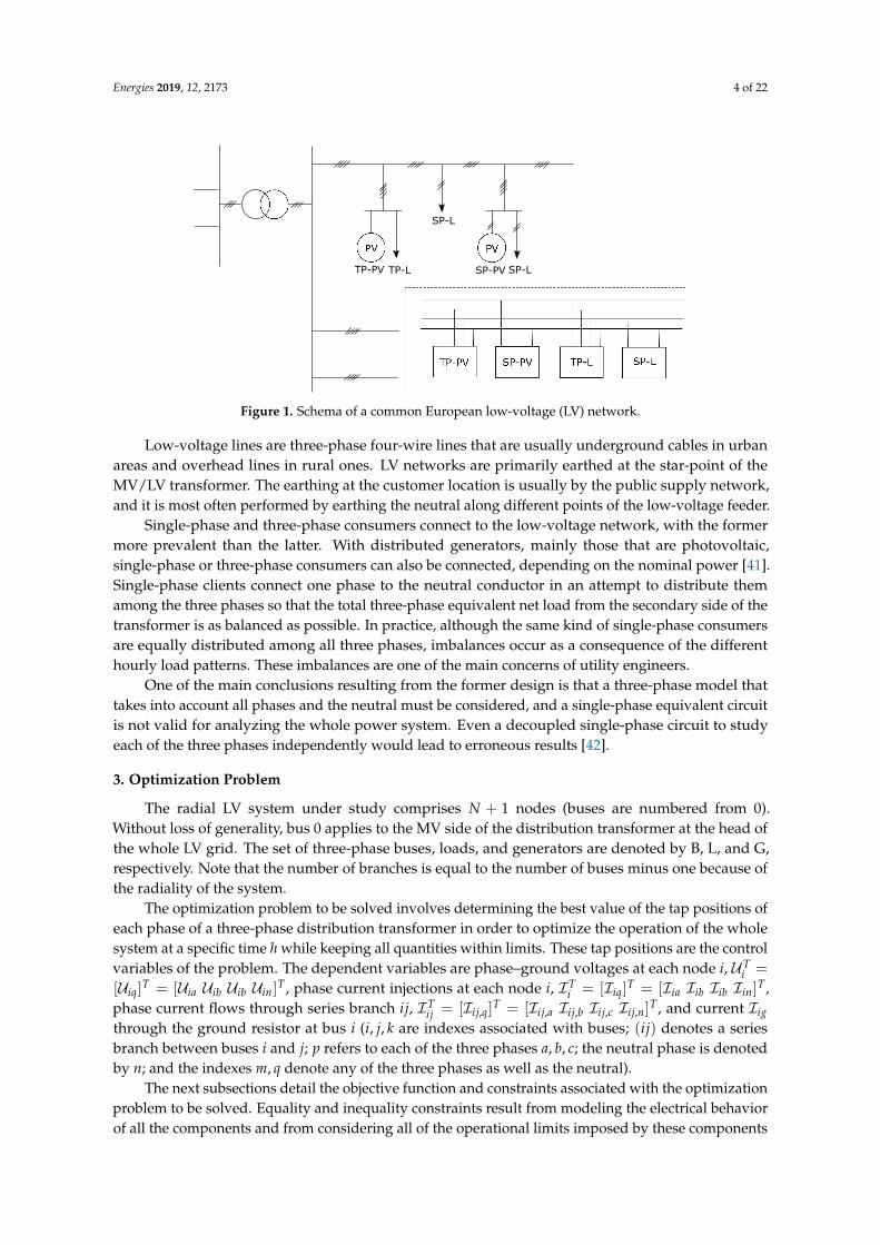
Distribution networks with the so-called European design are not limited to Europe; in fact, theyare widely used all over the world. Many other countries adopted this arrangement, and the Europeandesign is well established, even in urban North American distribution networks [40]. The generalstructure of European distribution systems consists of a three-phase medium-voltage system in whichthree phase distribution transformers are connected to feed a large number of consumers/distributedgenerators connected to the three-phase low-voltage grid. An LV network can have a radial, ring,or meshed structure, but most are operated radially. Figure 1 depicts the schema of a typical radialEuropean low-voltage grid.

Distribution or secondary transformers are large three-phase transformers (normally between100 and 1000 kVA), with 20 kV/400 V being the most typical normalized voltages. One of the mostcommon configurations is delta-wye because this arrangement prevents imbalance on the low-voltageside (due to unbalanced consumption) by transferring loads to the MV level. Nowadays, most of thesesecondary transformers have off-load tap changers, and OLTC transformers are considered in the restof the paper, as justified in Section 1.

Energies 2019, 12, 2173 4 of 22

TP-PV TP-L SP-PV SP-L

SP-L

Figure 1. Schema of a common European low-voltage (LV) network.

Low-voltage lines are three-phase four-wire lines that are usually underground cables in urbanareas and overhead lines in rural ones. LV networks are primarily earthed at the star-point of theMV/LV transformer. The earthing at the customer location is usually by the public supply network,and it is most often performed by earthing the neutral along different points of the low-voltage feeder.

Single-phase and three-phase consumers connect to the low-voltage network, with the formermore prevalent than the latter. With distributed generators, mainly those that are photovoltaic,single-phase or three-phase consumers can also be connected, depending on the nominal power [41].Single-phase clients connect one phase to the neutral conductor in an attempt to distribute themamong the three phases so that the total three-phase equivalent net load from the secondary side of thetransformer is as balanced as possible. In practice, although the same kind of single-phase consumersare equally distributed among all three phases, imbalances occur as a consequence of the differenthourly load patterns. These imbalances are one of the main concerns of utility engineers.

One of the main conclusions resulting from the former design is that a three-phase model thattakes into account all phases and the neutral must be considered, and a single-phase equivalent circuitis not valid for analyzing the whole power system. Even a decoupled single-phase circuit to studyeach of the three phases independently would lead to erroneous results [42].

3. Optimization Problem

The radial LV system under study comprises N + 1 nodes (buses are numbered from 0).Without loss of generality, bus 0 applies to the MV side of the distribution transformer at the head ofthe whole LV grid. The set of three-phase buses, loads, and generators are denoted by B, L, and G,respectively. Note that the number of branches is equal to the number of buses minus one because ofthe radiality of the system.

The optimization problem to be solved involves determining the best value of the tap positions ofeach phase of a three-phase distribution transformer in order to optimize the operation of the wholesystem at a specific time h while keeping all quantities within limits. These tap positions are the controlvariables of the problem. The dependent variables are phase–ground voltages at each node i, UT

i =

[Uiq]T = [Uia Uib Uib Uin]

T , phase current injections at each node i, ITi = [Iiq]

T = [Iia Iib Iib Iin]T ,

phase current flows through series branch ij, ITij = [Iij,q]

T = [Iij,a Iij,b Iij,c Iij,n]T , and current Iig

through the ground resistor at bus i (i, j, k are indexes associated with buses; (ij) denotes a seriesbranch between buses i and j; p refers to each of the three phases a, b, c; the neutral phase is denotedby n; and the indexes m, q denote any of the three phases as well as the neutral).

The next subsections detail the objective function and constraints associated with the optimizationproblem to be solved. Equality and inequality constraints result from modeling the electrical behaviorof all the components and from considering all of the operational limits imposed by these components

Energies 2019, 12, 2173 5 of 22

and the fulfillment of required standards. The phase domain and phase coordinates are consideredto set out the problem, with computations being performed in physical units. In what follows,each complex equation that appears should be transformed into two equivalent real equations; this stepis omitted throughout the paper.

3.1. Objective Function

The minimization of power losses is proposed as the main target objective. The power losses of thesystem can be formulated from a power balance point of view, so the following objective Function (1)results:

min <(Sloss) = min <(UT0 I∗0 ) +

N+1

∑i=1

∑p

[SG

ip + SLip

], (1)

where SGip refers to the generated specified power at phase p of node i, and SL

ip denotes the demandedcomplex power of a load at phase p of node i. Note the net injected power by shunt elements connectedto bus i is Sip = SG

ip + SLip, so the generated power SG

ip takes values greater than zero while the

demanded load SLip takes negative values. It is important to underline that the objective Function (1)

considers all losses, namely power losses in the transformer, lines, and ground resistors.The minimization of imbalances, voltage drops, or neutral currents are other common objective

functions to consider. Power losses have commonly been chosen since they represent a well-definedsingle key index whose lowest value is usually linked to the best voltage profile. Other possible choicesare those defined at a node or branch level, and such options necessitate the definition of a single indexfor any of them (for example, if the minimization of voltage drops was chosen, a possible voltageindex to quantify this objective could be the addition of the deviation of each node voltage from itsnominal value). In sum, an objective function that differs from the minimization of power losses couldbe set out.

3.2. Medium-Voltage Grid Equivalent

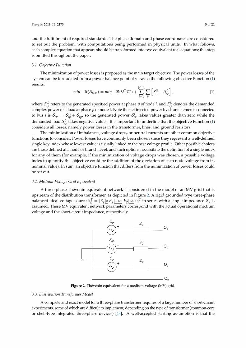
A three-phase Thévenin equivalent network is considered in the model of an MV grid that isupstream of the distribution transformer, as depicted in Figure 2. A rigid grounded wye three-phasebalanced ideal voltage source ET

g = [Eg |0 Eg |−120 Eg |120 0]T in series with a single impedance Zg isassumed. These MV equivalent network parameters correspond with the actual operational mediumvoltage and the short-circuit impedance, respectively.

g+

ga

Oa

g+

gb

Ob

g+

gc

Oc

On

Figure 2. Thévenin equivalent for a medium-voltage (MV) grid.

3.3. Distribution Transformer Model

A complete and exact model for a three-phase transformer requires of a large number of short-circuitexperiments, some of which are difficult to implement, depending on the type of transformer (common-coreor shell-type integrated three-phase devices) [43]. A well-accepted starting assumption is that the

Energies 2019, 12, 2173 6 of 22

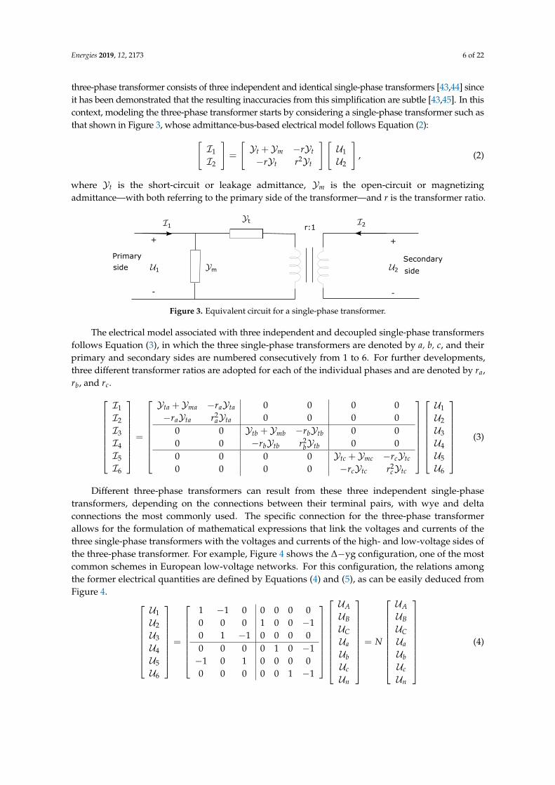
three-phase transformer consists of three independent and identical single-phase transformers [43,44] sinceit has been demonstrated that the resulting inaccuracies from this simplification are subtle [43,45]. In thiscontext, modeling the three-phase transformer starts by considering a single-phase transformer such asthat shown in Figure 3, whose admittance-bus-based electrical model follows Equation (2):[

I1

I2

]=

[Yt + Ym −rYt

−rYt r2Yt

] [U1

U2

], (2)

where Yt is the short-circuit or leakage admittance, Ym is the open-circuit or magnetizingadmittance—with both referring to the primary side of the transformer—and r is the transformer ratio.

r:1t

m

1

1

2

2

+

-

+

-

Secondary Primary

sideside

Figure 3. Equivalent circuit for a single-phase transformer.

The electrical model associated with three independent and decoupled single-phase transformersfollows Equation (3), in which the three single-phase transformers are denoted by a, b, c, and theirprimary and secondary sides are numbered consecutively from 1 to 6. For further developments,three different transformer ratios are adopted for each of the individual phases and are denoted by ra,rb, and rc.

I1

I2

I3

I4

I5

I6

=

Yta + Yma −raYta 0 0 0 0−raYta r2

aYta 0 0 0 00 0 Ytb + Ymb −rbYtb 0 00 0 −rbYtb r2

bYtb 0 00 0 0 0 Ytc + Ymc −rcYtc

0 0 0 0 −rcYtc r2cYtc

U1

U2

U3

U4

U5

U6

(3)

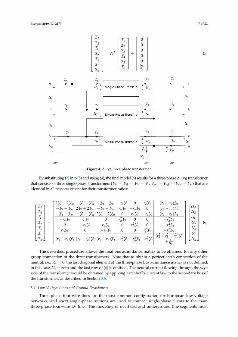
Different three-phase transformers can result from these three independent single-phasetransformers, depending on the connections between their terminal pairs, with wye and deltaconnections the most commonly used. The specific connection for the three-phase transformerallows for the formulation of mathematical expressions that link the voltages and currents of thethree single-phase transformers with the voltages and currents of the high- and low-voltage sides ofthe three-phase transformer. For example, Figure 4 shows the ∆−yg configuration, one of the mostcommon schemes in European low-voltage networks. For this configuration, the relations amongthe former electrical quantities are defined by Equations (4) and (5), as can be easily deduced fromFigure 4.

U1

U2

U3

U4

U5

U6

=

1 −1 0 0 0 0 00 0 0 1 0 0 −10 1 −1 0 0 0 00 0 0 0 1 0 −1−1 0 1 0 0 0 00 0 0 0 0 1 −1

UAUBUCUa

UbUc

Un

= N

UAUBUCUa

UbUc

Un

(4)

Energies 2019, 12, 2173 7 of 22

IAIBICIa

IbIc

In

= NT

I1

I2

I3

I4

I5

I6

+

00000UnRg

(5)

12

1+

-

+

-2

34

3+

-

+

-4

56

5+

-

+

-6

a

b

c

n

A

B

C

+

-n

A

B

C

A

+

-

B

+

C

+

a

+

-

b

+

c

+

a

b

c

n

g

g

Figure 4. ∆−yg three-phase transformer.

By substituting (3) into (5) and using (4), the final model (6) results for a three-phase ∆−yg transformerthat consists of three single-phase transformers (Yta = Ytb = Ytc = Yt, Yma = Ymb = Ymc = Ym) that areidentical in all respects except for their transformer ratios:

IAIBICIa

IbIc

In

=

2Yt + 2Ym −Yt −Ym −Yt −Ym −raYt 0 rcYt (ra − rc)Yt

−Yt −Ym 2Yt + 2Ym −Yt −Ym raYt −rbYt 0 (rb − ra)Yt

−Yt −Ym −Yt −Ym 2Yt + 2Ym 0 rbYt −rcYt (rc − rb)Yt

−raYt raYt 0 r2aYt 0 0 −r2

aYt

0 −rbYt rbYt 0 r2bYt 0 −r2

bYt

rcYt 0 −rcYt 0 0 r2cYt −r2

cYt

(ra − rc)Yt (rb − ra)Yt (rc − rb)Yt −r2aYt −r2

bYt −r2cYt

(r2a + r2

b + r2c )Yt

+ 1Rg

UAUBUCUa

UbUc

Un

(6)

The described procedure allows the final bus admittance matrix to be obtained for any othergroup connection of the three transformers. Note that to obtain a perfect earth connection of theneutral, i.e., Rg = 0, the last diagonal element of the three-phase bus admittance matrix is not defined;in this case, Un is zero and the last row of (6) is omitted. The neutral current flowing through the wyeside of the transformer would be obtained by applying Kirchhoff’s current law to the secondary bus ofthe transformer, as described in Section 3.6.

3.4. Low-Voltage Lines and Ground Resistances

Three-phase four-wire lines are the most common configuration for European low-voltagenetworks, and short single-phase sections are used to connect single-phase clients to the mainthree-phase four-wire LV line. The modeling of overhead and underground line segments must

Energies 2019, 12, 2173 8 of 22

be as precise as possible since this model plays an important role in the final solution, as illustratedlater. This high accuracy demands for a complete and reliable database in relation to low-voltage lines:the type and size of every conductor, the physical geometry of both overhead and underground lines,the resistance of the earth, etc. This information allows Carsons’s equations [46] to be applied in orderto obtain the resistance and the self- and mutual inductive reactance of the conductors that make upthe line. These series impedances are shown in Figure 5. A 4 × 4 series impedance matrix Zij resultsfrom this model (7). The series impedance matrix is completely full for a three-phase four-wire line,with only non-null elements in one phase and neutral positions for two-phase or single-phase lines.

Ui = ZijIij + Uj =

UiaUibUicUin

=

Z aa

ij Z abij Z ac

ij Z anij

Z abij Zbb

ij Zbcij Zbn

ijZ ac

ij Zbcij Z cc

ij Z cnij

Z anij Zbn

ij Z cnij Znn

ij

Iij,aIij,bIij,cIij,n

+

UjaUjbUjcUjn

(7)

ja

jb

jc

jn

ia

ib

ic

Zaaij

Zcc

Znn

Zan

Zbc

Zcn

Zab

Zac

Zan

U ib

U ia

U ic

U in

U ja

U jb

U jc

U jn

Iij,a

Iij,b

Iij,c

Iij,n

RigRjg

Zbbij

ij ij ij

ij

ij

ij

ij

ij

in

Figure 5. Three-phase four-wire electric line model.

It is common practice to neglect capacitances in the case of low-voltage lines because the lengthsof the lines are short. So, throughout this paper, this shunt effect is not considered.

It is not always possible to apply Carson’s equations because the requisite information is not usuallyavailable in utility-based data (distance between conductors, height of conductors, earth resistivity, etc.).Instead, positive sequence impedance Z1 and, more rarely, zero sequence impedance Z0 are the onlypracticable line data. In this last case, the best-approximated series impedance ZAprox

ij is

ZAproxij =

Z1 0 0 00 Z1 0 00 0 Z1 0

0 0 0Z0 −Z1

3

. (8)

This simplified model is obtained by assuming an identical type of conductor for all phasesand the neutral and equal sections, symmetrical spacing between phases (including the neutral),and perfect earthing at both extremes of each line segment [46].

Neutral conductors are commonly grounded at multiple points along the network (neutralgrounding) for safety reasons. The values of these resistors depend on the type of earth conductorand electrode, as well as the resistivity of the terrain. These characteristics determine the value of the

Energies 2019, 12, 2173 9 of 22

resistor Rig to consider at each bus i, and the value can ideally move between zero and infinity. If thisresistor is a finite value, Ohm’s law is applied (9):

Uin = RigIig ∀ bus i earthed with a finite resistor, (9)

where Iig denotes the current flowing through the ground resistor. Note that Uin has a null result forrigid earthing.

If the neutral of bus i is not connected to the ground, that is, Rig = ∞, the ground current is forcedto be zero (10):

Iig = 0 ∀ bus i unearthed (10)

3.5. Loads and Renewable Generators

Hereinafter, the appropriate model for consumers and renewable generators connected to thelow-voltage system is discussed. The optimal power flow analysis discussed throughout this paperdeals with the steady state, so static models are considered.

Static load models can be classified into the following groups: exponential, polynomial, linear,comprehensive, static induction motor, and power electronic-interfaced models [47]. Among all thesestatic load models, the constant real and reactive power load model is the most widely used forutilities [47], as a particular case of the polynomial or ZIP model (constant impedance Z, constantcurrent I, and constant power P model). Any other model could be considered if the appropriateparameters for each load are known. For renewable generation, with a focus on PV technologies,a steady-state power injection model is also adopted. PV generators operate by injecting the maximumavailable power, which varies depending on the irradiance. Similarly, the reactive power injection canbe set depending on the standing grid code. Unity power factor operation is a common practice for PVgenerators connected to LV networks.

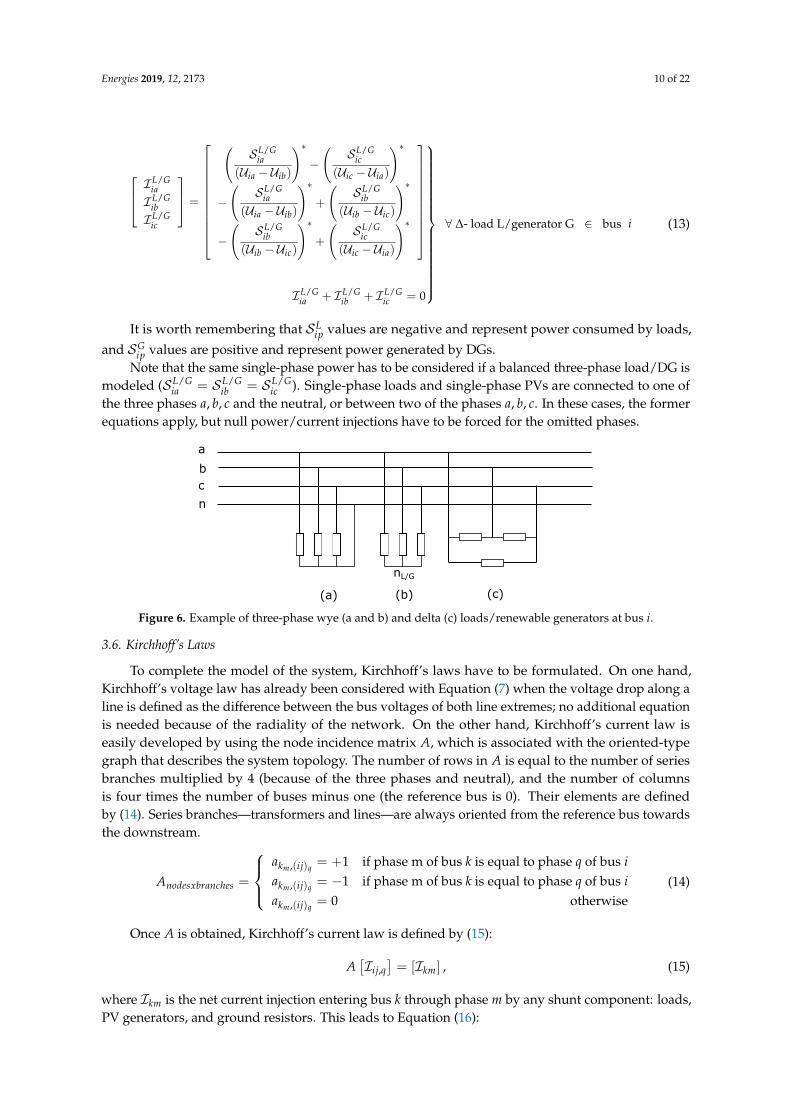
Three-phase loads and generators can be connected in wye or delta configurations, as shown inFigure 6. The neutral can be accessible or inaccessible in wye connections, and they are referred to as athree-phase four-wire connection or three-phase three-wire connection, respectively (see Figure 6a,b).The electrical model is given by (11) for a three-phase four-wire load/generator connected to bus i,while (12) is applicable to a three-phase four-wire load/generator.

SL/GiaSL/G

ibSL/G

ic

=

(Uia −Uin)(IL/Gia )∗

(Uib −Uin)(IL/Gib )∗

(Uic −Uin)(IL/Gic )∗

IL/Gia + IL/G

ib + IL/Gic + IL/G

in = 0

∀ Three-phase four-wire - load L/ generator G ∈ bus i (11)

SL/GiaSL/G

ibSL/G

ic

=

(Uia −UinL/G)(IL/G

ia )∗

(Uib −UinL/G)(IL/G

ib )∗

(Uic −UinL/G)(IL/G

ic )∗

IL/Gia + IL/G

ib + IL/Gic = 0

∀ Three-phase three-wire wye- load L/ generator G ∈

bus i ,(12)

where L/G refers to the chosen load (L) or generator (G), depending on the considered component.Equation (13) defines delta-connected three-phase loads or generators.

Energies 2019, 12, 2173 10 of 22

IL/GiaIL/G

ibIL/G

ic

=

(SL/G

ia(Uia −Uib)

)∗−(

SL/Gic

(Uic −Uia)

)∗

−(

SL/Gia

(Uia −Uib)

)∗+

(SL/G

ib(Uib −Uic)

)∗

−(

SL/Gib

(Uib −Uic)

)∗+

(SL/G

ic(Uic −Uia)

)∗

IL/Gia + IL/G

ib + IL/Gic = 0

∀ ∆- load L/generator G ∈ bus i (13)

It is worth remembering that SLip values are negative and represent power consumed by loads,

and SGip values are positive and represent power generated by DGs.

Note that the same single-phase power has to be considered if a balanced three-phase load/DG ismodeled (SL/G

ia = SL/Gib = SL/G

ic ). Single-phase loads and single-phase PVs are connected to one ofthe three phases a, b, c and the neutral, or between two of the phases a, b, c. In these cases, the formerequations apply, but null power/current injections have to be forced for the omitted phases.

a

b

c

n

(a) (b)

nL/G

(c)

Figure 6. Example of three-phase wye (a and b) and delta (c) loads/renewable generators at bus i.

3.6. Kirchhoff’s Laws

To complete the model of the system, Kirchhoff’s laws have to be formulated. On one hand,Kirchhoff’s voltage law has already been considered with Equation (7) when the voltage drop along aline is defined as the difference between the bus voltages of both line extremes; no additional equationis needed because of the radiality of the network. On the other hand, Kirchhoff’s current law iseasily developed by using the node incidence matrix A, which is associated with the oriented-typegraph that describes the system topology. The number of rows in A is equal to the number of seriesbranches multiplied by 4 (because of the three phases and neutral), and the number of columnsis four times the number of buses minus one (the reference bus is 0). Their elements are definedby (14). Series branches—transformers and lines—are always oriented from the reference bus towardsthe downstream.

Anodesxbranches =

akm ,(ij)q = +1 if phase m of bus k is equal to phase q of bus iakm ,(ij)q = −1 if phase m of bus k is equal to phase q of bus iakm ,(ij)q = 0 otherwise

(14)

Once A is obtained, Kirchhoff’s current law is defined by (15):

A[Iij,q

]= [Ikm] , (15)

where Ikm is the net current injection entering bus k through phase m by any shunt component: loads,PV generators, and ground resistors. This leads to Equation (16):

Energies 2019, 12, 2173 11 of 22

[Ikp

]= ∑L,G∈k

([IG

kp

]+[IL

kp

])Ikn = IG

kn + ILkn − Ikg

∀ bus k (16)

3.7. Operational Constraints

Secure operation of the system requires that voltage quantities remain within limits. This meansthat two inequality constraints are applied for each phase-neutral voltage at each bus. Therefore, upperand lower limits, Vmax and Vmin, respectively, are imposed:(

Vmin)2≤(Vip −Vin

)2 ≤ (Vmax)2 ∀ i, p = a, b, c (17)

Note that the constraint (17) is formulated in a quadratic form to avoid square roots, which causestrong nonlinearity in the resulting optimization problem.

4. Simulation Results

This section presents the results obtained for a benchmark European low-voltage network [48]when the optimal voltage control is achieved using 1P-OLTCST or 3P-OLTCST. The main objectivesare to show the benefits of using decoupled tap control compared with traditional uniform three-phasetap control and illustrate the importance of the model in carrying out effective control.

The main aim of each optimization problem, 1P-OLTCST or 3P-OLTCST, is to provide a feasiblesolution regarding the fixed voltage bounds while minimizing the power losses of the system andfulfilling the power flow equations. If there is no solution that meets the voltage limit constraints,the solver provides the optimal solution without taking into account the lower voltage limit to avoidthe non-convergence of the optimization problem.

This section is organized as follows: Section 4.1 presents the tested network and someconsiderations to take into account in the analysis; next, Sections 4.2 and 4.3 not only compare the twomeans of control (1P-OLTCST or 3P-OLTCST) for a specific load scenario but also demonstrate theimportance of accuracy for the line model and earthing configuration. Finally, Section 4.4 incorporatesdistributed generation and compares both control strategies for a daily power scenario of both loadsand generators.

4.1. Example Scenario Settings

In the subsequent simulations, let us consider the LV distribution network shown in Figure 7.In this grid, a three-phase medium-voltage system is connected to a three-phase low-voltage gridthrough the use of MV/LV transformers. The LV network has a radial structure in which threetypes of feeders are contemplated according to the connected consumers: residential, industrial,and commercial. Daily load profiles and detailed models of the different underground and overheadlow-voltage lines considered in this work are provided in [48].

The following considerations apply in all the tested cases:

• In our study, a unique transformer MV/LV that feeds the three aforementioned subsystems isconsidered. The configuration of the transformer is ∆−yg, and its nominal values are listed inTable 1. Short-circuit impedance Zt refers to the MV primary side of the transformer.

• Slack bus, on the high-voltage side of the transformer, is assumed to be the nominal 20 kV, so anideal three-phase wye voltage source is considered.

• A single tap is considered for each phase of the three-phase distribution transformer whendecoupled tap control is applied (1P-OLTCST), while these three single taps move equally whenthe traditional three-phase control is considered (3P-OLTCST). Each tap has nine positions betweenthe limits 0.92 and 1.08, in steps of 0.02.

Energies 2019, 12, 2173 12 of 22

• The nominal phase-neutral voltage is V = 400/√

3 V, and the Spanish normative is adopted withregard to voltage limits, that is, ±7% of Vn, which corresponds to a maximum phase-neutralvoltage of 247.1 V and a minimum of 214.8 V.

• Loads and renewable generators are modeled as constant power, with a wye three-phase four-wireconfiguration in the case of three-phase control; single-phase loads are connected between one ofthe three phases a, b, c and the neutral.

• All study cases were modeled using Python, and the stated optimization problem was solved with SciPy.

0

1

R

R

R

R

R R R

R

R

R

R

R

R

RR

R

R

I

C

CC

C

C

C

C

C

C C C

CC

C

C

C

C

C C

Residential subnetwork Commercial subnetwork

Industrial subnetwork

Figure 7. Modified European low-voltage benchmark network [48].

Table 1. Transformer parameters for the considered scenario.

Bus from Bus to Connection V1 [kV] V2 [kV] Zt [Ω] Srated [kVA]

0 1 ∆−yg 20 0.4 21.164 + j69.616 630

4.2. Line Modeling Accuracy

Let us consider (1) the load configuration detailed in Table 2 for a given time and (2) the neutralground configuration shown in Table 3. Table 2 specifies the apparent load power demanded ateach bus (negative values imply that power is not injected but consumed), power factor, and thepercentage of the apparent power corresponding to each of the three phases and for every load bus.This unbalanced load scenario supposes that the total power demanded upstream is 319.85 kW and118.78 kvar (without considering power losses) and that the proportions of the active power at each ofthe three phases a, b, and c are 32.07%, 22.73%, and 44.2%, respectively. This scenario is not excessivelyimbalanced, although phase c is more loaded, to the detriment of phase b.

Below, the optimization problem detailed in Section 3 is solved for the specified load scenarioand earthing configuration. The two control strategies (1P-OLTCST and 3P-OLTCST) are not onlyconsidered but also solved if the exact line model provided in [48] is assumed (7) or if there are

Energies 2019, 12, 2173 13 of 22

insufficient line data and a simplified model (s.m.) is the only possibility (8). Table 4 gives thesimulation results for all four cases, as well as the base case corresponding to the nominal positionof the taps, and once again, an exact line model or the approximated line model is used. The mainfigures are the phase transformer ratio, total active power losses (and savings in losses in percentagerelative to the base case), and maximum and minimum phase-neutral voltages in the system (redfigures are used to emphasize quantities out of limits). For those voltage controls assuming a simplifiedmodel, two quantities are reported for each magnitude: that obtained by the approximated model andthe equivalent real value linked to the exact model (this last one between brackets), both computedwith the optimal tap positions obtained by the corresponding optimization problem. For each typeof transformer, the optimal solutions obtained are not the same when considering an accurate or asimplified model of the power lines. This fact makes the solver provide two different results for thetransformer taps.

Table 2. Load configuration.

Bus R2 R11 R15 R16 R17 R18 I2 C2

S [kVA] −12 −55 −25 −100 −44 −10 −15 −10

cos ϕ 0.95 0.95 0.95 0.95 0.95 0.95 0.85 0.95

Ph. a (%) 20 30 40 40 35 40 0 0Ph. b (%) 20 20 30 10 25 20 70 70Ph. c (%) 60 50 30 50 40 40 30 30

Bus C8 C12 C13 C14 C17 C18 C19 C20

S [kVA] −8 −5 −20 −3 −12 −7 −10 −6

cos ϕ 0.90 0.90 0.90 0.90 0.90 0.90 0.90 0.90

Ph. a (%) 20 20 30 20 50 25 20 30Ph. b (%) 10 20 40 45 20 0 30 10Ph. c (%) 70 60 30 35 30 75 50 60

Table 3. Neutral ground configuration.

Bus 1 R4 R6 R8 R10 R11 R15 R16 R17 R18 I2 C3

Rg(Ω) 3 40 40 40 40 40 40 40 40 40 40 40

Bus C5 C7 C9 C11 C12 C13 C14 C16 C17 C18 C19 C20

Rg(Ω) 40 40 40 40 40 40 40 40 40 40 40 40

It is worth pointing out that the 3P-OLTCST is not able to provide a feasible solution because thevoltages of some buses under the lower limit are fixed in the problem formulation. However, the samecase is efficiently solved by using a 1P-OLTCST that, relying on an independent tap position for eachphase, maintains the voltage of all the buses within limits, in addition to notably improving the powerlosses, reducing them by almost 15%, which is 6 points more than when using the 3P-OLTCST. Weemphasize the need for rigorousness in the model to be solved since it is evident from Table 4 thatsimplified line models fail to accurately comply with voltage constraints (note that maximum voltagesare greater than the upper limit of 247.1). Moreover, simplified models prevent obtaining an optimalsolution for tap positions, regardless of whether a three-phase OLTC or a single-phase OLTC for eachphase is considered.

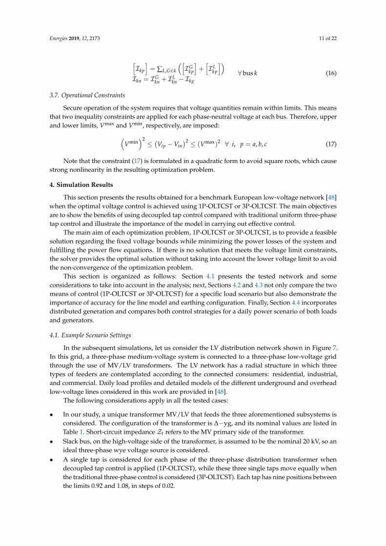
Figure 8 shows the phase-neutral voltages and neutral voltage at all buses for the 1P-OLTCSTfor both an accurate model and a simplified model of power lines. Figure 9 is the counterpart ofFigure 8 for the 3P-OLTCST. It is easily deduced by their comparison that the 1P-OLTCST phase-neutralvoltages become more balanced than those reached by the 3P-OLTCST, and the maximum voltagedrop is quite a bit lower in the first case, with values of 23.3 V and 32.6 V at the residential feeder for

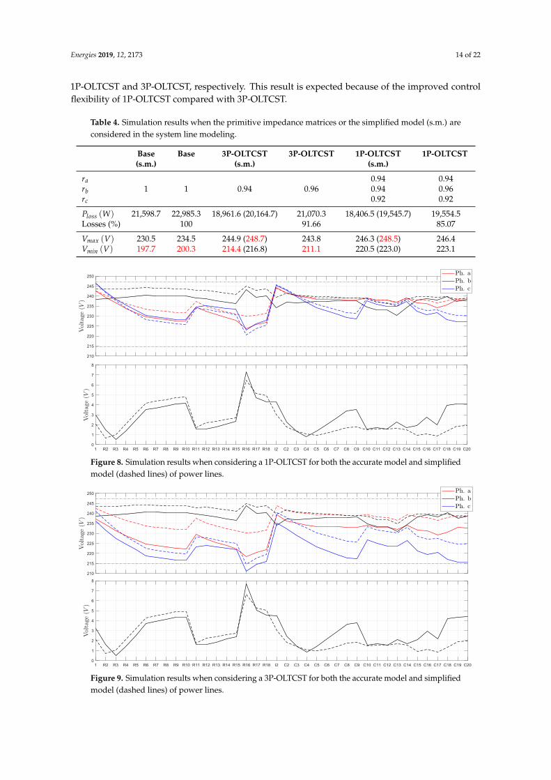
Energies 2019, 12, 2173 14 of 22

1P-OLTCST and 3P-OLTCST, respectively. This result is expected because of the improved controlflexibility of 1P-OLTCST compared with 3P-OLTCST.

Table 4. Simulation results when the primitive impedance matrices or the simplified model (s.m.) areconsidered in the system line modeling.

Base Base 3P-OLTCST 3P-OLTCST 1P-OLTCST 1P-OLTCST(s.m.) (s.m.) (s.m.)

ra1 1 0.94 0.96

0.94 0.94rb 0.94 0.96rc 0.92 0.92

Ploss (W) 21,598.7 22,985.3 18,961.6 (20,164.7) 21,070.3 18,406.5 (19,545.7) 19,554.5Losses (%) 100 91.66 85.07

Vmax (V) 230.5 234.5 244.9 (248.7) 243.8 246.3 (248.5) 246.4Vmin (V) 197.7 200.3 214.4 (216.8) 211.1 220.5 (223.0) 223.1

210

215

220

225

230

235

240

245

250

1 R2 R3 R4 R5 R6 R7 R8 R9 R10 R11 R12 R13 R14 R15 R16 R17 R18 I2 C2 C3 C4 C5 C6 C7 C8 C9 C10 C11 C12 C13 C14 C15 C16 C17 C18 C19 C20

0

1

2

3

4

5

6

7

8

Figure 8. Simulation results when considering a 1P-OLTCST for both the accurate model and simplifiedmodel (dashed lines) of power lines.

210

215

220

225

230

235

240

245

250

1 R2 R3 R4 R5 R6 R7 R8 R9 R10 R11 R12 R13 R14 R15 R16 R17 R18 I2 C2 C3 C4 C5 C6 C7 C8 C9 C10 C11 C12 C13 C14 C15 C16 C17 C18 C19 C20

0

1

2

3

4

5

6

7

8

Figure 9. Simulation results when considering a 3P-OLTCST for both the accurate model and simplifiedmodel (dashed lines) of power lines.

Energies 2019, 12, 2173 15 of 22

4.3. Ground Configuration

In this second case study, the effects of the neutral ground configuration on the optimal tappositions, system losses, and network voltage values are shown. Let us consider the same loadconfiguration as in the previous section (Table 2) but with different ground resistances.

Table 5. Neutral ground resistances at each bus.

Bus 1 R4 R6 R8 R10 R11 R15 R16 R17 R18 I2 C3

Rg(Ω) 3 R1 R2 R1 R2 R1 R2 R1 R2 R1 R1 R2

Bus C5 C7 C9 C11 C12 C13 C14 C16 C17 C18 C19 C20

Rg(Ω) R1 R2 R1 R2 R1 R2 R1 R2 R1 R2 R1 R2

From Table 5, the sequel ground configurations are analyzed:

• Case 1: Neutral resistor of finite value: R1 = R2 = 40 Ω.• Case 2: Neutral rigid earthing: R1 = R2 = 0 Ω.• Case 3: Neutral resistor of finite value: R1 = R2 = 3 Ω.• Case 4: Mixed earthing: R1 = 40 Ω, R2 = 0 Ω.

Table 6 shows the simulation results for the four cases and for both types of control transformers,as well as the solutions for each case when the tap positions remain at their nominal values, forcomparison purposes. We highlight that the optimal transformer taps are the same for all cases,except for the one in which a rigid earthing of the neutral is considered (Case 2), and for both typesof control transformers. It can be seen that the results for a neutral grounding with a resistor of 3 Ω(Case 3) and a resistor of 40 Ω (Case 1) are very similar. However, only the 1P-OLTCST is able tomaintain the voltage within the prescribed limits since the 3P-OLTCST is not able to satisfy voltagelimits for any non-null value of grounding resistors. It is also noticeable that the 1P-OLTCST improvesthe power losses by around a 6% compared with the 3P-OLTCST in almost all cases. This improvementis reduced to 2.5% in the case of rigid grounding.

Table 6. Simulation results for different neutral ground configurations.

1P-OLTCST

Case 1 Case 2 Case 3 Case 4

1P 3P 1P 3P 1P 3P 1P 3POLTCST OLTCST OLTCST OLTCST OLTCST OLTCST OLTCST OLTCST

ra 0.94 0.94 0.94 0.94rb 0.96 0.96 0.94 0.94 0.96 0.96 0.96 0.96rc 0.92 0.92 0.92 0.92

Ploss (W) 19,554.548 21,070.299 18,607.972 19,172.366 19,494.120 21,003.3412 19,201.089 20,673.079Losses (%) 85.07 91.66 85.23 87.81 85.09 91.67 85.17 91.70

Vmax (V) 246.386 243.764 246.335 245.358 246.387 243.552 246.376 243.013Vmin (V) 223.084 211.088 222.224 216.103 223.182 211.199 222.896 210.921

3P-OLTCST

Case 1 Case 2 Case 3 Case 4

ra1 1 1 1rb

rc

Ploss (W) 22,985.288 21,831.880 22,910.126 22,544.249Losses (%) 100 100 100 100

Vmax (V) 234.531 230.955 234.310 233.746Vmin (V) 200.288 199.543 200.406 200.106

Energies 2019, 12, 2173 16 of 22

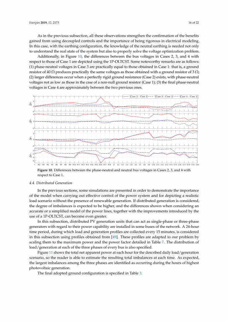
As in the previous subsection, all these observations strengthen the confirmation of the benefitsgained from using decoupled controls and the importance of being rigorous in electrical modeling.In this case, with the earthing configuration, the knowledge of the neutral earthing is needed not onlyto understand the real state of the system but also to properly solve the voltage optimization problem.

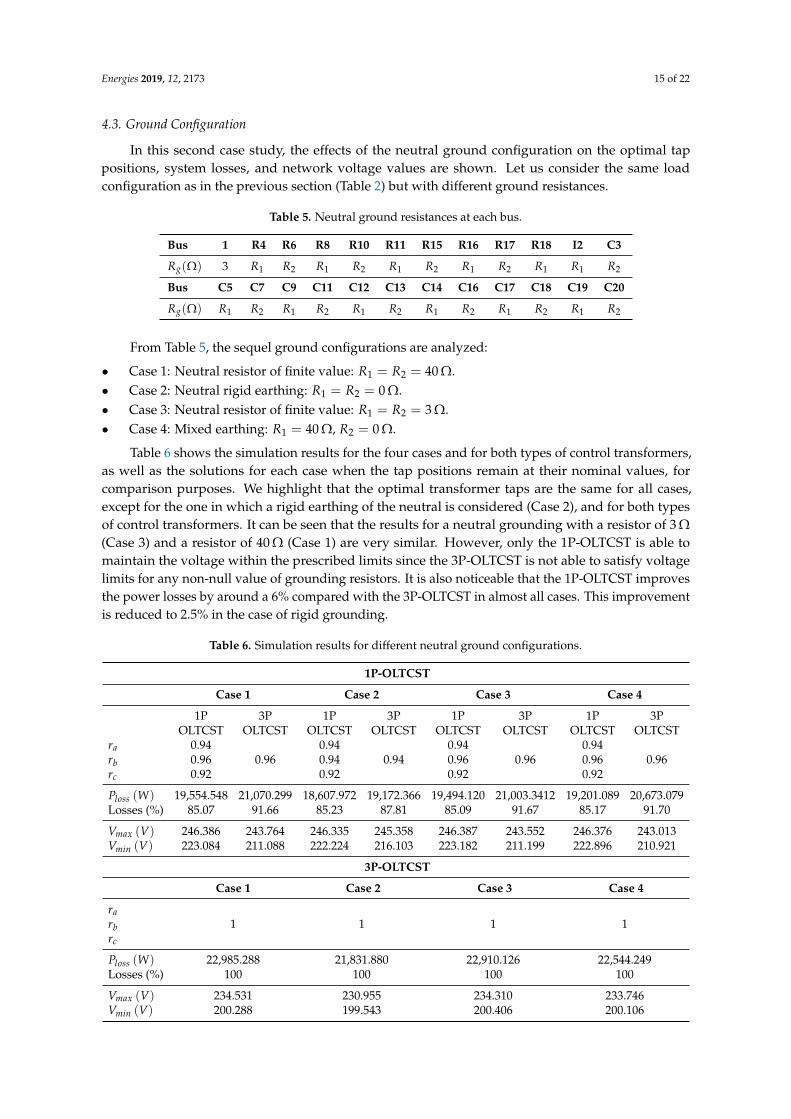
Additionally, in Figure 10, the differences between the bus voltages in Cases 2, 3, and 4 withrespect to those of Case 1 are depicted using the 1P-OLTCST. Some noteworthy remarks are as follows:(1) phase-neutral voltages in Case 3 are practically equal to those obtained in Case 1: that is, a groundresistor of 40 Ω produces practically the same voltages as those obtained with a ground resistor of 3 Ω;(2) larger differences occur when a perfectly rigid ground resistance (Case 2) exists, with phase-neutralvoltages not as low as those in the case of a non-null ground resistor (Case 1); (3) the final phase-neutralvoltages in Case 4 are approximately between the two previous ones.

-2

0

2

4

-5

0

5

-2

0

2

1 R2 R3 R4 R5 R6 R7 R8 R9 R10 R11 R12 R13 R14 R15 R16 R17 R18 I2 C2 C3 C4 C5 C6 C7 C8 C9 C10 C11 C12 C13 C14 C15 C16 C17 C18 C19 C20

-6

-4

-2

0

( ( ( ( ( (

Figure 10. Differences between the phase-neutral and neutral bus voltages in Cases 2, 3, and 4 withrespect to Case 1.

4.4. Distributed Generation

In the previous sections, some simulations are presented in order to demonstrate the importanceof the model when carrying out effective control of the power system and for depicting a realisticload scenario without the presence of renewable generation. If distributed generation is considered,the degree of imbalances is expected to be higher, and the differences shown when considering anaccurate or a simplified model of the power lines, together with the improvements introduced by theuse of a 1P-OLTCST, can become even greater.

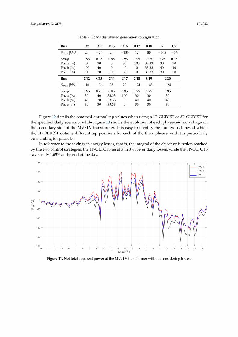
In this subsection, distributed PV generation units that can act as single-phase or three-phasegenerators with regard to their power capability are installed in some buses of the network. A 24-hourtime period, during which load and generation profiles are collected every 15 minutes, is consideredin this subsection using profiles obtained from [49]. These profiles are adapted to our problem byscaling them to the maximum power and the power factor detailed in Table 7. The distribution ofload/generation at each of the three phases of every bus is also specified.

Figure 11 shows the total net apparent power at each hour for the described daily load/generationscenario, so the reader is able to estimate the resulting total imbalances at each time. As expected,the largest imbalances among the three phases are identified as occurring during the hours of highestphotovoltaic generation.

The final adopted ground configuration is specified in Table 3.

Energies 2019, 12, 2173 17 of 22

Table 7. Load/distributed generation configuration.

Bus R2 R11 R15 R16 R17 R18 I2 C2

Smax [kVA] 20 −75 25 −135 17 80 −105 −36

cos ϕ 0.95 0.95 0.95 0.95 0.95 0.95 0.95 0.95Ph. a (%) 0 30 0 30 100 33.33 30 30Ph. b (%) 100 40 0 40 0 33.33 40 40Ph. c (%) 0 30 100 30 0 33.33 30 30

Bus C12 C13 C14 C17 C18 C19 C20

Smax [kVA] −101 −36 35 20 −24 −48 −24

cos ϕ 0.95 0.95 0.95 0.95 0.95 0.95 0.95Ph. a (%) 30 40 33.33 100 30 30 30Ph. b (%) 40 30 33.33 0 40 40 40Ph. c (%) 30 30 33.33 0 30 30 30

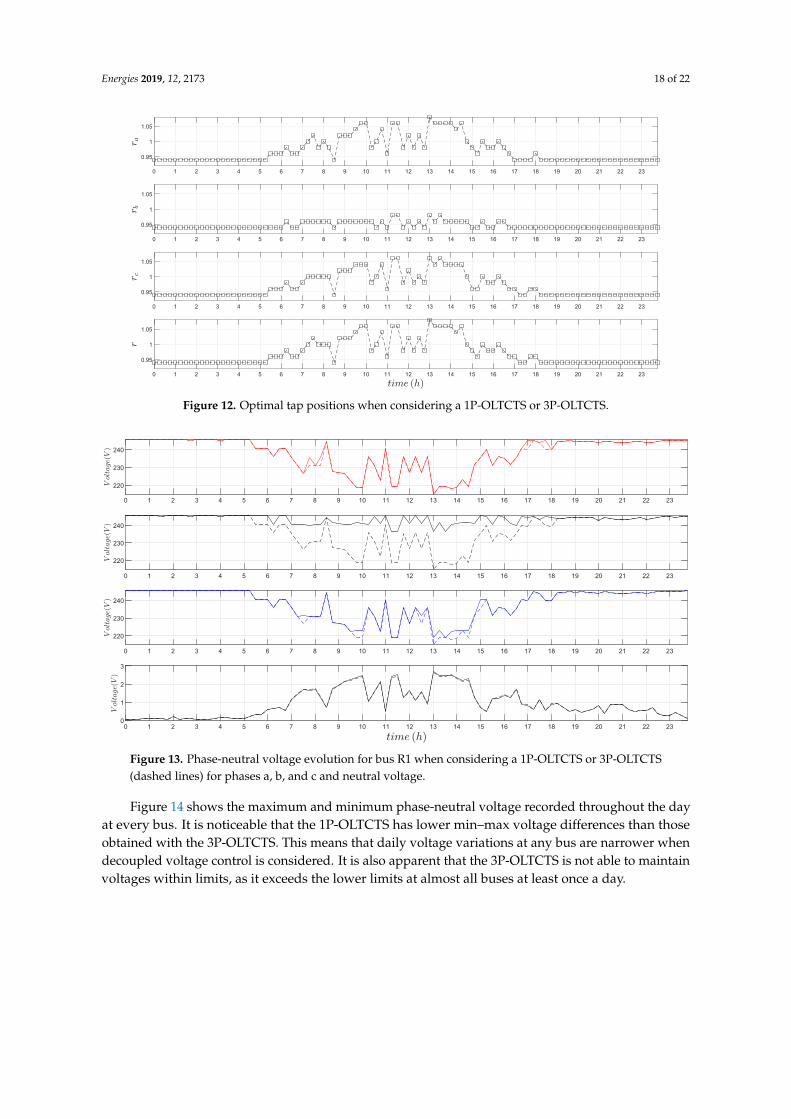
Figure 12 details the obtained optimal tap values when using a 1P-OLTCST or 3P-OLTCST forthe specified daily scenario, while Figure 13 shows the evolution of each phase-neutral voltage onthe secondary side of the MV/LV transformer. It is easy to identify the numerous times at whichthe 1P-OLTCST obtains different tap positions for each of the three phases, and it is particularlyoutstanding for phase b.

In reference to the savings in energy losses, that is, the integral of the objective function reachedby the two control strategies, the 1P-OLTCTS results in 3% lower daily losses, while the 3P-OLTCTSsaves only 1.05% at the end of the day.

0 1 2 3 4 5 6 7 8 9 10 11 12 13 14 15 16 17 18 19 20 21 22 23

-100

-80

-60

-40

-20

0

20

40

60

80

Figure 11. Net total apparent power at the MV/LV transformer without considering losses.

Energies 2019, 12, 2173 18 of 22

0 1 2 3 4 5 6 7 8 9 10 11 12 13 14 15 16 17 18 19 20 21 22 23

0.95

1

1.05

0 1 2 3 4 5 6 7 8 9 10 11 12 13 14 15 16 17 18 19 20 21 22 23

0.95

1

1.05

0 1 2 3 4 5 6 7 8 9 10 11 12 13 14 15 16 17 18 19 20 21 22 23

0.95

1

1.05

0 1 2 3 4 5 6 7 8 9 10 11 12 13 14 15 16 17 18 19 20 21 22 23

0.95

1

1.05

Figure 12. Optimal tap positions when considering a 1P-OLTCTS or 3P-OLTCTS.

0 1 2 3 4 5 6 7 8 9 10 11 12 13 14 15 16 17 18 19 20 21 22 23

220

230

240

0 1 2 3 4 5 6 7 8 9 10 11 12 13 14 15 16 17 18 19 20 21 22 23

220

230

240

0 1 2 3 4 5 6 7 8 9 10 11 12 13 14 15 16 17 18 19 20 21 22 23

220

230

240

0 1 2 3 4 5 6 7 8 9 10 11 12 13 14 15 16 17 18 19 20 21 22 230

1

2

3

Figure 13. Phase-neutral voltage evolution for bus R1 when considering a 1P-OLTCTS or 3P-OLTCTS(dashed lines) for phases a, b, and c and neutral voltage.

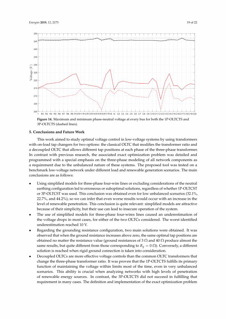
Figure 14 shows the maximum and minimum phase-neutral voltage recorded throughout the dayat every bus. It is noticeable that the 1P-OLTCTS has lower min–max voltage differences than thoseobtained with the 3P-OLTCTS. This means that daily voltage variations at any bus are narrower whendecoupled voltage control is considered. It is also apparent that the 3P-OLTCTS is not able to maintainvoltages within limits, as it exceeds the lower limits at almost all buses at least once a day.

Energies 2019, 12, 2173 19 of 22

1 R2 R3 R4 R5 R6 R7 R8 R9 R10R11R12R13R14R15R16R17R18 I2 C2 C3 C4 C5 C6 C7 C8 C9 C10C11C12C13C14C15C16C17C18C19C20

200

205

210

215

220

225

230

235

240

245

250

Figure 14. Maximum and minimum phase-neutral voltage at every bus for both the 1P-OLTCTS and3P-OLTCTS (dashed lines).

5. Conclusions and Future Work

This work aimed to study optimal voltage control in low-voltage systems by using transformerswith on-load tap changers for two options: the classical OLTC that modifies the transformer ratio anda decoupled OLTC that allows different tap positions at each phase of the three-phase transformer.In contrast with previous research, the associated exact optimization problem was detailed andprogrammed with a special emphasis on the three-phase modeling of all network components asa requirement due to the unbalanced nature of these systems. The proposed tool was tested on abenchmark low-voltage network under different load and renewable generation scenarios. The mainconclusions are as follows:

• Using simplified models for three-phase four-wire lines or excluding considerations of the neutralearthing configuration led to erroneous or suboptimal solutions, regardless of whether 1P-OLTCSTor 3P-OLTCST was used. This conclusion was obtained even for low unbalanced scenarios (32.1%,22.7%, and 44.2%), so we can infer that even worse results would occur with an increase in thelevel of renewable penetration. This conclusion is quite relevant: simplified models are attractivebecause of their simplicity, but their use can lead to insecure operation of the system.

• The use of simplified models for three-phase four-wires lines caused an underestimation ofthe voltage drops in most cases, for either of the two OLTCs considered. The worst identifiedunderestimation reached 10 V.

• Regarding the grounding resistance configuration, two main solutions were obtained. It wasobserved that when the ground resistance increases above zero, the same optimal tap positions areobtained no matter the resistance value (ground resistances of 3 Ω and 40 Ω produce almost thesame results, but quite different from those corresponding to Rg = 0 Ω). Conversely, a differentsolution is reached when rigid ground connection is taken into consideration.

• Decoupled OLTCs are more effective voltage controls than the common OLTC transformers thatchange the three-phase transformer ratio. It was proven that the 1P-OLTCTS fulfills its primaryfunction of maintaining the voltage within limits most of the time, even in very unbalancedscenarios. This ability is crucial when analyzing networks with high levels of penetrationof renewable energy sources. In contrast, the 3P-OLTCTS did not succeed in fulfilling thatrequirement in many cases. The definition and implementation of the exact optimization problem

Energies 2019, 12, 2173 20 of 22

carried out throughout this work was essential to come to this conclusion and would have notbeen possible if approximated models had been assumed.

• Besides more effectively maintaining voltage within limits and having lower power losses,the 1P-OLTCTS had lower voltage drops and daily voltage variation than the 3P-OLTCTS. For thetested cases, the best saving in power losses was 85.1% for the 1P-OLTCTS, versus 91.7% for the3P-OLTCTS; the highest voltage drop was 4.5% for the 1P-OLTCTS, versus 9% for the 3P-OLTCTS;and the maximum daily voltage variation was reduced by up to more than 10 V with 1P-OLTCTSversus 3P-OLTCTS.

Future work will examine the coupling of all time frameworks under study in order to reduce thenumber of movements of tap positions and to maximize the lifetime of the device; it is clear that suchtap movements do not lead to profitable savings of power losses and although voltages are withinlimits, tap movements should be avoided. In addition, the current work focused on the decoupledOLTC as the only means of voltage control in order to understand its real possibilities and because it isa solution that is close to the current reality of utilities. However, additional voltage controls, such asstatcoms, inverters linked to renewable generators, or storage systems, would be interesting to studyin future analyses.

Author Contributions: Conceptualization, Á.R.d.N., E.R.-R., and Á.L.T.-G.; Formal analysis, Á.R.d.N., E.R.-R.,and Á.L.T.-G.; Validation, Á.R.d.N., E.R.-R., and Á.L.T.-G.; Writing—original draft, Á.R.d.N., E.R.-R., and Á.L.T.-G.

Funding: The authors would like to acknowledge the financial support of the Spanish Ministry of Economyand Competitiveness under grants ENE2014-54115-R and ENE2017-84813-R and the CDTI Grant PASTORA-ITC-20181102 (Innterconecta program, partially FEDER Technology Fund).

Conflicts of Interest: The authors declare no conflict of interest.

References

1. Country Fiches for Electricity Smart Metering Accompanying the Document Report from the CommissionBenchmarking Smart Metering Deployment in the EU-27 with a Focus on Electricity; Commission Staff WorkingDocument; Publications Office of the European Union: Brussels, Belgium, 2014.

2. International Energy Agency (IEA). IRENA Cost and Competitiveness Indicators: Rooftop solar PV; IEAPublications: Paris, France, December 2017.

3. International Energy Agency (IEA). Global EV Outlook 2017. Two Milllion and Counting; IEA Publications:Paris, France, 2017.

4. Gozel, T.; Ochoa, L.F. Deliverable 3.3 (Updated) Performance evaluation of the monitored LV networks.In Electricity North West Limited (ENWL)—Low Voltage Network Solutions; The University of Manchester:Manchester, UK, July 2014.

5. Mohammadi, P.; Mehraeen, S. Challenges of PV Integration in Low-Voltage Secondary Networks. IEEE Trans.Power Deliv. 2017, 32, 525–535.

6. Noske, S.; Falkowski, D.; Swat, K.; Boboli, T. UPGRID project: The management and control of LV network.CIRED-Open Access Proc. J. 2017, 2017, 1520–1522. [CrossRef]

7. Poursharif, G.; Brint, A.; Black, M.; Marshall, M. Analysing the ability of smart meter data to provide accurateinformation to the UK DNOs. CIRED-Open Access Proc. J. 2017, 2017, 2078–2081.

8. Wong, P.K.C.; Barr, R.; Kalam, A. Analysis of voltage quality data from smart meters. In Proceedingsof the 22nd Australasian Universities Power Engineering Conference (AUPEC), Bali, Indonesia, 26–29September 2012.

9. Wong, P.K.C.; Barr, R.; Kalam, A. A big data challenge—Turning smart meter voltage quality data intoaionable information. In Proceedings of the 22nd International Conference on Electricity Distribution(CIRED), Stockholm, Sweden, 10–13 June 2013.

10. Prado, J.G.; González, A.; Riaño, S. Adopting smart meter events as key data for low-voltage networkoperation. CIRED-Open Access Proc. J. 2017, 2017, 924–928. [CrossRef]

Energies 2019, 12, 2173 21 of 22

11. Navarro, A.; Ochoa, L.F.; Mancarella, P.; Randles, D. Impacts of photovoltaics on low voltage networks:A case study for the North West of England. In Proceedings of the 22nd International Conference onElectricity Distribution (CIRED), Stockholm, Sweden, 10–13 June 2013.

12. Report C1: Use of smart meter information for network planning and operation. In UK Power NetworksHoldings Limited—Low Carbon London Project; UK Power Networks Holdings Limited: London, UK,September 2014.

13. Seymour, J. The Seven Types of Power Problems. White Paper 18, Revision 1, Schneider Electric—Data Center,Science Center. 2011. Available online: http://www.apc.com/salestools/VAVR-5WKLPK/VAVR-5WKLPK_R1_EN.pdf (accessed on 1 May 2019).

14. O’Connell, A.; Soroudi, A.; Keane, A. Distribution Network Operation Under Uncertainty Using InformationGap Decision Theory. IEEE Trans. Smart Grid 2018, 9, 1848–1858.

15. Lan, B.-R.; Chang, C.-A.; Huang, P.-Y.; Kuo, C.-H.; Ye, Z.-J.; Shen, B.-C.; Chen, B.-K. Conservation voltageregulation (CVR) applied to energy savings by voltage-adjusting equipment through AMI. IOP Conf. Ser.Earth Environ. Sci. 2017, 93, 012070. [CrossRef]

16. Nijhuis, M.; Gibescu, M.; Cobben, J.F.G. Valuation of measurement data for low voltage network expansionplanning. Electr. Power Syst. Res. 2017, 151, 59–67. [CrossRef]

17. Aziz, T.; Ketjoy, N. PV Penetration Limits in Low Voltage Networks and Voltage Variations. IEEE Access2017, 5, 16784–16792.

18. Tahir, M.; Nassar, M.E.; El-Shatshat, R.; Salama, M.M.A. A review of Volt/Var control techniques in passiveand active power distribution networks. In Proceedings of the 4th IEEE International Conference on SmartEnergy Grid Engineering (SEGE), Oshawa, ON, Canada, 21–24 August 2016; pp. 57–63.

19. Bayer, B.; Matschoss, P.; Thomas, H.; Marian, A. The German experience with integrating photovoltaicsystems into the low-voltage grids. Renew. Energy 2018, 119, 129–141. [CrossRef]

20. Yan, R.; Marais, B.; Saha, T.K. Impacts of residential photovoltaic power fluctuation on on-load tap changeroperation and a solution using DSTATCOM. Electr. Power Syst. Res. 2014, 111, 185–193. [CrossRef]

21. Long, C.; Ochoa, L.F. Voltage Control of PV-Rich LV Networks: OLTC-Fitted Transformer and CapacitorBanks. IEEE Trans. Power Syst. 2016, 31, 4016–4025. [CrossRef]

22. Coppo, M.; Turri, R.; Marinelli, M.; Han, X. Voltage management in unbalanced low voltage networks usinga decoupled phase-tap-changer transformer. In Proceedings of the 49th International Universities PowerEngineering Conference (UPEC), Cluj-Napoca, Romania, 2–5 September 2014; pp. 1–6.

23. Zecchino, A.; Marinelli, M.; Hu, J.; Coppo, M.; Turri, R. Voltage control for unbalanced low voltage gridsusing a decoupled-phase on-load tap-changer transformer and photovoltaic inverters. In Proceedings of the50th International Universities Power Engineering Conference (UPEC), Stoke on Trent, UK, 1–4 September2015; pp. 1–6.

24. Hu, J.; Marinelli, M.; Coppo, M.; Zecchino, A.; Bindner, H.W. Coordinated voltage control of a decoupledthree-phase on-load tap changer transformer and photovoltaic inverters for managing unbalanced networks.Electr. Power Syst. Res. 2016, 131, 264–274. [CrossRef]

25. Zecchino, A.; Hu, J.; Coppo, M.; Marinelli, M. Experimental testing and model validation of adecoupled-phase on-load tap-changer transformer in an active network. IET Gen. Transm. Distrib. 2016, 10,3834–3843. [CrossRef]

26. Quirós-Tortós, J.; Ochoa, L.F.; Alnaser, S.W.; Butler, T. Control of EV Charging Points for Thermal and VoltageManagement of LV Networks. IEEE Trans. Power Syst. 2016, 31, 3028–3039. [CrossRef]

27. Efkarpidis, N.; Rybel, T.D.; Driesen, J. Optimal Placement and Sizing of Active In-Line Voltage Regulators inFlemish LV Distribution Grids. IEEE Trans. Ind. Appl. 2016, 52, 4577–4584. [CrossRef]

28. Procopiou, A.T.; Ochoa, L.F. Voltage Control in PV-Rich LV Networks Without Remote Monitoring.IEEE Trans. Power Syst. 2017, 32, 1224–1236. [CrossRef]

29. Pezeshki, H.; Arefi, A.; Ledwich, G.; Wolfs, P. Probabilistic Voltage Management Using OLTC anddSTATCOM in Distribution Networks. IEEE Trans. Power Deliv. 2017, 33, 570–580. [CrossRef]

30. Fallahzadeh-Abarghouei, H.; Nayeripour, M.; Hasanvand, S.; Waffenschmidt, E. Online hierarchical anddistributed method for voltage control in distribution smart grids. IET Gen. Transm. Distrib. 2017, 11,1223–1232 [CrossRef]

31. Aziz, T.; Ketjoy, N. Enhancing PV Penetration in LV Networks Using Reactive Power Control and On LoadTap Changer with Existing Transformers. IIEEE Access 2018, 6, 2683–2691. [CrossRef]

Energies 2019, 12, 2173 22 of 22

32. Bettanin, A.; Coppo, M.; Savio, A.; Turri, R. Voltage management strategies for low voltage networks suppliedthrough phase-decoupled on-load-tap-changer transformers. In Proceedings of the AEIT InternationalAnnual Conference, Cagliari, Italy, 20–22 September 2017; pp. 1–6.

33. Jiricka, J.; Kaspirek, M.; Kolar, L.; Zahradka, M. Smart Substation MV/LV. In Proceedings of the 24thInternational Conference on Electricity Distribution (CIRED), Glasgow, UK, 12–15 June 2017; pp. 1–5.

34. Baudot, C.; Roupioz, G.; Carre, O.; Wild, J.; Potet, C. Experimentation of voltage regulation infrastructureon LV network using an OLTC with a PLC communication system. CIRED-Open Access Proc. J. 2017, 2017,1120–1122. [CrossRef]

35. Mokkapaty, S.; Weiss, J.; Schalow, F.; Declercq, J. New generation voltage regulation distribution transformerwith an on load tap changer for power quality improvement in the electrical distribution systems.CIRED-Open Access Proc. J. 2017, 2017, 784–787. [CrossRef]

36. Daratha, N.; Das, B.; Sharma, J. Coordination Between OLTC and SVC for Voltage Regulation in UnbalancedDistribution System Distributed Generation. IEEE Trans. Power Syst. 2014, 29, 289–299. [CrossRef]

37. Frame, D.; Bell, K.; McArthur, S. A Review and Synthesis of the Outcomes from Low Carbon NetworksFund Projects. UKERK Publications. August 2016. Available online: http://www.ukerc.ac.uk/publications/a-review-and-synthesis-of-the-outcomes-from-low-carbon-networks-fund-projects.html (accessed on1 May 2019).

38. Chen, T.-H.; Yang, W.-C. Analysis of multi-grounded four-wire distribution systems considering the neutralgrounding. IEEE Trans. Power Deliv. 2001, 16, 710–717. [CrossRef]

39. Urquhart, A.J. Accuracy of Low Voltage Electricity Distribution Network Modelling. Ph.D. Thesis,Loughborough Universtiy, Loughborough, UK, 2016.

40. Willis, H. L. Power Distribution Planning Reference Book, 2nd ed.; CRC Press: Boca Raton, FL, USA, March2004; ISBN 978-0824748753.

41. Özkan, Z.; Hava, A.M. Three-phase inverter topologies for grid-connected photovoltaic systems.In Proceedings of the International Power Electronics Conference (IPEC), Hiroshima, Japan, 18–21 May 2014;pp. 498–505.

42. Moreno-Díaz, L.; Romero-Ramos, E.; Gómez-Expósito, A.; Cordero-Herrera, E.; Rivero, J.R.; Cifuentes, J.S.Accuracy of Electrical Feeder Models for Distribution Systems Analysis. In Proceedings of the InternationalConference on Smart Energy Systems and Technologies (SEST), Sevilla, Spain, 10–12 September 2018; pp. 1–6.

43. Chen, M.S.; Dillon, W.E. Power system modeling. Proc. IEEE 1974, 62, 901–915. [CrossRef]44. Rodas, R.D.E.; Padilha-Feltrin, A.; Ochoa, L.F. Distribution transformers modeling with angular

displacement: Actual values and per unit analysis. SBA Controle & Automação Sociedade Brasileira de Automatica2007, 18, 499–500.

45. Carneiro, S.; Martins, H.J.A. Measurements and model validation on three-phase core-type distributiontransformers. In Proceedings of the IEEE Power Engineering Society General Meeting, Toronto, ON, Canada,13–17 March 2004; pp. 120–124.

46. Kersting, W.H. Distribution System Modeling and Analysis, 3rd ed.; CRC Press: Boca Raton, FL, USA,February 2016.

47. Modelling and Aggregation of Loads in Flexible Power Networks; Working Group C4.605; CIGRÉ, ConseilInternational des Grands Réseaux éLectriques: Paris, France, February 2014.

48. Benchmark Systems for Network Integration of Renewable and Distributed Energy Resources; Comité d’études C6;CIGRÉ, Conseil international des grands réseaux électriques: Paris, France, 2014.

49. Gozel, T.; Navarro, A.; Ochoa, L.F. Deliverable 3.5 Creation of Aggregated Profiles with and without NewLoads and DER Based on Monitored Data. April 2014. Available online: https://www.enwl.co.uk/zero-Carbon/smaller (accessed on 1 May 2019).

c© 2019 by the authors. Licensee MDPI, Basel, Switzerland. This article is an open accessarticle distributed under the terms and conditions of the Creative Commons Attribution(CC BY) license (http://creativecommons.org/licenses/by/4.0/).