acedp hydrology indicator report

RIVER HEALTH ASSESSMENT IN CHINA:

COMPARISON AND DEVELOPMENT OF

INDICATORS OF HYDROLOGICAL HEALTH

Prepared by the Chinese Research Academy of Environmental Sciences, the Pearl

River Water Resources Commission and the International WaterCentre

Australia-China Environment Development Partnership

River Health and Environmental Flow in China

Project Code: P0018

September 2011

i

Document History and Status

Version Date Issued Prepared by Reviewed by

A 15 January 2011 Chris Gippel and others Angela Arthington

B 01 April 2011 Chris Gippel Robert Speed

C 26 April 2011 Chris Gippel Nick Bond

D 17 June 2011 Chris Gippel Steering Committee

Final 29 Sep 2011 Chris Gippel Steering Committee

Distribution

Version Date Issued Method Issued to

A 15 January 2011 Email .pdf and .docx Robert Speed

B 01 April 2011 Email .pdf and .docx Robert Speed

C 26 April 2011 Email .pdf and .docx Robert Speed

D 17 June 2011 Email .pdf and .docx Robert Speed

Final 29 Sep 2011 Email .pdf and .docx Robert Speed

Document Management

Printed Not printed

Last saved 29 September 2011

File name C:\...\09010_ACEDP_China\Reports\Hydrology Indicators\ACEDP Hydrology Indicator

Report_Final_29102011.docx

Authors Christopher Gippel, Zhang Yuan, Qu Xiaodong, Kong Weijing, Nick Bond, Liu Wei

Organisation International WaterCentre Pty Ltd

Document name Comparison and development of indicators of hydrological health

Document version Final

Suggested citation:

Gippel, C.J., Zhang, Y., Qu, X., Kong, W., Bond, N.R., Jiang, X. and Liu, W. 2011. River health assessment in

China: comparison and development of indicators of hydrological health. ACEDP Australia-China Environment

Development Partnership, River Health and Environmental Flow in China. The Chinese Research Academy of

Environmental Sciences, the Pearl River Water Resources Commission and the International WaterCentre,

Brisbane, September.

For further information on any of the information contained within this document contact:

International WaterCentre Pty Ltd

PO Box 10907, Adelaide St

Brisbane, Qld, 4000

Tel: +61 7 31237766

Email: [email protected]

www.watercentre.org

This publication may be of assistance to you, but the International Water Centre and its employees and

contractors do not guarantee that the publication is without flaw of any kind, or is wholly appropriate for your

particular purposes and therefore disclaims all liability for any error, loss or other consequence which may arise

from you relying on information in this publication.

mailto:[email protected]

http://www.watercentre.org/

ii

About this document

This document is one of a series of technical papers prepared to support work on the ACEDP River

Health and Environmental Flow in China Project.

The project objectives were to document and trial, in China, international approaches to river health and

environmental flows assessment. The trial involved three pilot river basins – the Yellow, Pearl and Liao

River Basins. Further details on the pilot projects can be found in the River Health and Environmental

Flow in China Inception Report, 16 December 2010.

The methodology described and applied in this paper is a component of the Liao, Pearl and Lower

Yellow river pilot studies. The results of the hydrological indicator work were used in the report cards for

the Liao and Pearl river pilots. The methods developed here are expected to have widespread

application in China and other countries.

iii

Contents

About this document ............................................................................................................................................ ii

Contents ............................................................................................................................................................... iii

Abstract ................................................................................................................................................................ vi

Introduction ........................................................................................................................................................... 1

Brief Introduction to the Gui, Taizi and Lower Yellow Rivers ........................................................................... 2

Gui River (Pearl River Basin) .............................................................................................................................. 2

Taizi River (Liao River Basin) ............................................................................................................................. 3

Lower Yellow River (Yellow River Basin) ............................................................................................................ 4

Hydrological Data .................................................................................................................................................. 5

Available flow series ........................................................................................................................................... 5

Flow regulation periods ....................................................................................................................................... 6

Definition of water year and seasons .................................................................................................................. 7

Index of Flow Stress (FSR) ................................................................................................................................... 9

Flow Stress Ranking (FSR) Indicators ................................................................................................................ 9

Application of the FSR to Chinese case studies ............................................................................................... 13

Calculation procedure .................................................................................................................................. 13

FSR application to the Taizi River ..................................................................................................................... 14

FSR application to the Gui River....................................................................................................................... 18

FSR application to the Yellow River .................................................................................................................. 20

Discussion of FSR indicators ............................................................................................................................ 20

Chinese Hydrology and Water Resources Index (HD) ..................................................................................... 23

Introduction ....................................................................................................................................................... 23

Methodology ..................................................................................................................................................... 24

Flow variation degree (FD) ........................................................................................................................... 24

Satisfaction level of ecological flow (EF) ...................................................................................................... 25

Constraints on application of HD .................................................................................................................. 26

Definition of water year and seasons ........................................................................................................... 26

Results (FD)...................................................................................................................................................... 27

Gui River system .......................................................................................................................................... 27

Lower Yellow River ....................................................................................................................................... 27

Overall result for FD ..................................................................................................................................... 29

Results (EF) ...................................................................................................................................................... 30

Taizi River .................................................................................................................................................... 30


Gui River system .......................................................................................................................................... 33

Results (HD) ..................................................................................................................................................... 34


Gui River system .......................................................................................................................................... 35

iv

Discussion of HD index ..................................................................................................................................... 35

Index of Flow Deviation (IFD) ............................................................................................................................. 38

Introduction ....................................................................................................................................................... 38

Principles ...................................................................................................................................................... 38

Flow Health software .................................................................................................................................... 38

Scoring according to the natural range of variability ..................................................................................... 38

Definition of water year and seasons ........................................................................................................... 40

Indicators .......................................................................................................................................................... 40

High flow volume (HFV) and low flow volume (LFV) .................................................................................... 41

Highest monthly flow (HMF) and lowest monthly flow (LMF) ........................................................................ 42

Persistently higher flow (PHF) ...................................................................................................................... 43

Persistently lower flow (PLF) ........................................................................................................................ 43

Persistently very low (PVL) ........................................................................................................................... 44

Seasonality flow shift (SFS) .......................................................................................................................... 45

Index of Flow Deviation (IFD) ....................................................................................................................... 45

Example IFD Calculation (Liaoyang, year 2000)............................................................................................... 46

Step 1: Determine reference period ............................................................................................................. 46

Step 2: Determine the water year ................................................................................................................. 46

Step 3: Establish the reference distributions and thresholds ........................................................................ 46

Step 4: Calculate indicator scores ................................................................................................................ 49

Results .............................................................................................................................................................. 53

Taizi River .................................................................................................................................................... 53

Gui River ...................................................................................................................................................... 53


Correlation of IFD and HD indicators ................................................................................................................ 70

Intercorrelation of IFD indicators .................................................................................................................. 70

Intercorrelation of HD indicators ................................................................................................................... 70

Correlation between IFD and HD indicators ................................................................................................. 74

Modelled reference versus historical reference ............................................................................................ 77

The connection between IFD and environmental flows .................................................................................... 79

Discussion of IFD index .................................................................................................................................... 80

Index of Flow Health (IFH) Based on Locally Assessed Environmental Flow Requirements – Taizi River 84

Introduction ....................................................................................................................................................... 84

Background hydrological information ................................................................................................................ 84

River regulation ............................................................................................................................................ 84

Data availability ............................................................................................................................................ 85

Flow seasonality and water year .................................................................................................................. 86

Flow regulation periods ................................................................................................................................ 88

Impact of dam regulation on overall flow pattern .......................................................................................... 88

Methodology ..................................................................................................................................................... 88

v

Previous environmental flow assessments in the Taizi River ........................................................................... 92

Characterisation of flow components ................................................................................................................ 95

Baseflows ..................................................................................................................................................... 95

Cease to flow events .................................................................................................................................... 98

Flow events (pulses and floods) ................................................................................................................... 98

Rates of rise and fall ................................................................................................................................... 109

Eco-hydraulic information ............................................................................................................................... 110

Data from cross-section locations .............................................................................................................. 110

Hydraulic data ............................................................................................................................................ 118

Comprehensive environmental flow objectives ............................................................................................... 124

Introduction ................................................................................................................................................. 124

Development of geomorphological flow objectives ..................................................................................... 125

Development of vegetation flow objectives................................................................................................. 139

Development of fish flow objectives ........................................................................................................... 140

Development of macroinvertebrate flow objectives .................................................................................... 141

Comprehensive flow objectives .................................................................................................................. 143

Flow magnitudes associated with the flow objectives ..................................................................................... 150

Evaluation of the hydraulic and hydrological criteria ....................................................................................... 150

Results ............................................................................................................................................................ 154

Correlation of IFH indicators ........................................................................................................................... 159

Intercorrelation of IFH indicators ................................................................................................................ 159

Correlation between IFH and IFD and HD indicators ................................................................................. 159

Relationship between IFH and IFD and HD indicators ............................................................................... 163

Discussion of IFH index .................................................................................................................................. 163

Discussion and Conclusion ............................................................................................................................. 165

References ......................................................................................................................................................... 168

Appendix A. Biological Information for Fish of the Taizi River ..................................................................... 180

vi

Abstract

As a component of the Australia China Environment Development Program (ACEDP) River Health and

Environmental Flow in China Project, this report developed and trialled methods suitable for characterising the

hydrology of the Taizi (Liao River Basin), Gui (Pearl River Basin) and Lower Yellow (Yellow River Basin) rivers in

a way that has direct meaning for ecological health. Four contrasting approaches to hydrological characterisation

were taken:

1. Application of an existing rapid method of characterising hydrological alteration, with the method

adopted here being the Flow Stress Ranking (FSR) procedure

2. Application of the Chinese Hydrology and Water Resources Index (HD), which has been proposed for a

nation-wide river health assessment program

3. Development of a suit of flow deviation indicators based on historical monthly flows, which here was

termed the Index of Flow Deviation (IFD)

4. Development of a method that used environmental flows compliance testing as a river health index,

which here was termed the Index of Flow Health (IFH)

The IFH approach offers a fundamentally different way of assessing hydrology compared to that followed by the

FSR, HD and IFD approaches. The FSR, HD and IFD approaches attempt to answer for a test year, or test

period:

“Do general hydrological parameters, thought to be either universally important or universally

undesirable for maintaining good river health, have characteristics that are different to those of the

reference (natural or unimpaired) flow regime?”

The IFH approach attempts to answer the question for a test year, or test period:

“To what degree do specific hydrological parameters, identified as either locally important or locally

undesirable for maintaining river health to an agreed standard, occur in the current flow regime?”

In this report, the FSR, HD and IFD methods were applied in the three test rivers, while the IFH was applied only

in the Taizi River. It is planned to apply the IFH in the Lower Yellow and Li (Gui River catchment) rivers in 2011.

The FSR indicators are relatively easy to calculate from monthly flows, and they show sensitivity to hydrological

alteration. However, the results can be difficult to interpret in terms of river health impacts, and do not necessarily

assist in deciding the most appropriate course of management action. Another problem is that the method ideally

requires simulated reference and current flow series, which are not generally available in China. If applied to a

gauged flow series, the indicators only indicate the broad impact of regulation on flows over a period of time.

Without the availability of output from frequently updated hydrological models, the method cannot realistically

contribute to an annual river health report card.

The HD index proposed for China’s nation-wide river health assessment program suffers some limitations in

terms of where it can be applied. The HD index has two sub-indicators, FD (Flow variation Degree) and EF

(Ecological Flow). In general, application of the HD method would be limited to rivers with modelled reference

flows, because these flows are required for calculation of the FD indicator. Where simulated reference flows are

available, the models are unlikely to be current in most places. The EF indicator is ideally calculated from a daily

flow series, which is not always readily available in China, further limiting the applicability of the HD index. The

FD indicator, which is based on the AAPFD index, was a good indicator of the volume of water diverted from the

river, but the conceptual link to ecosystem health was weak. The EF indicator is grounded in the simple Tennant

concept of relating hydrological factoring to ecosystem health. Inclusion of EF in China’s nation-wide river health

assessment program requires review. The root causes of the failure of the EF indicator are: (i) the weakness of

the assumptions involved in transfer of the Tennant method to rivers beyond those where the method was

originally devised, (ii) the limited concept of what constitutes a suitable flow regime for ecosystem protection

vii

embodied in the Tennant method, and (iii) no conceptual link between the indicator score for a year (derived from

the flow that occurred on one particular day of the year) and ecological health for that year.

To overcome the demonstrated limitations of the FSR and HD approaches in China, the IFD was developed to

measure flow alteration based on comparison with pre-regulation monthly flow data. The IFD was designed to

work with monthly historical flow data. It comprises eight indicators, with each one having conceptual relevance

to ecosystem health. The IFD, with its focus on highlighting deviations of flow parameters beyond a reasonable

range of natural variability, proved to be adequate as a river health index. The IFD highlights impacts of flow

regulation, and also highlights years of naturally lower than usual flows, both of which are important determinants

of ambient ecological health, as measured using bioassessment methods. At the very least, the IFD provides a

simple way of establishing the relative hydrological health of rivers at the national and regional scales for gauging

stations that have pre-regulation flow data available. When the IFD concept was developed as a software

application, it was renamed Flow Health.

Although the IFD was not intended, and is not recommended, for use as an environmental flow design tool, it

could be used in this way. If all eight IFD indicators are satisfied, the recommended monthly flows would

constitute a reasonably high percentage of the reference flows (65 – 71% of MAF for the Taizi River). However,

such flow recommendations should always be regarded as preliminary, and used only for planning purposes

rather than for developing water release schedules.

Given that the IFD is a hydrology-only approach, and the monthly time-step is relatively coarse from the

perspective of ecological processes, the connection between the index scores and ecological health is only at the

conceptual level. Thus, an Index of Flow Health (IFH) based on locally assessed environmental flow

requirements was developed. The IFH is measured as the degree of compliance of environmental flow

components with the standards expected for an agreed level of ecological stream health.

The stream health standards for the IFH were determined for the Taizi River within an environmental flows

assessment framework using a mix of expert opinion and flow-habitat and flow-geomorphology relationships from

the literature. There are no suitable ecological data available from the Taizi River to validate these standards for

local conditions because: (i) the river has been regulated for a long time, so recent ecological survey data reflect

regulated conditions, and (ii) there are a number of factors other than flow that compromise stream health, such

as poor water quality, barriers, and gravel extraction, so the influence of flow alteration on ecology is confounded.

The environmental flow assessment undertaken for the Taizi River main stem used the asset-based framework

set out in the ACEDP River Health and Environmental Flow in China Project. Flow objectives were set for

vegetation, fish, macroinvertebrates and physical form. Flow event objectives were specified in multi-dimensional

terms of magnitude, duration, annual frequency and inter-annual frequency, so a sophisticated form of spells

analysis was undertaken to determine the compliance of the flow components. Compliance means the frequency

that components appeared in the flow regime, relative to the frequency required to achieve the agreed level of

river health. The evaluation of the compliance of the suite of core environmental flow components produced a

comprehensive picture of the pattern of flow health in the Taizi River main stem over the past 50 years.

Compliance with expected was high for all flow components for the pre-dam periods at each station, although

there were a few exceptions. Regulation by dams caused a dramatic decline in the IFH scores. Liaoyang, just

downstream of two large dams with another much larger dam further upstream, was arguably the most seriously

hydrologically impacted reach.

The IFH requires more effort than simple computation of indicators from a hydrological data series. Work is

required to understand the hydraulic and hydrological characteristics of the river under investigation, and also to

define river health in terms of the particular hydraulic and hydrological needs of the local ecological assets. This

is standard procedure for a holistic environmental flow assessment. In this report it was demonstrated how useful

information can be derived on these subjects using existing data and expertise. In rivers where a comprehensive

environmental flow assessment has already been undertaken, the IFH can simply be calculated from hydrological

records.

The IFH index approach to assessment of stream hydrology for river health assessment has a number of

significant advantages over other simpler approaches, including:

viii

Each of the indicators has an explicit link to ecosystem health, in particular those aspects related to the

key ecological assets.

The reference standards are not related to pristine hydrology, which in many places would be regarded

as unachievable, and perhaps not relevant. Rather, the hydrological standards are set according to the

desired state of ecological health, as determined using a scientific process.

The index is expressed in terms that relate directly to those aspects of the flow regime that are

manageable through implementation of an environmental flow regime. Thus, scores will reflect positive

management intervention.

The main difficulty of deriving the IFH scores is not calculation of the scores per se, which requires only simple

algebra, but derivation of the environmental flow recommendations. Undertaking a holistic assessment of

environmental flow needs is not a trivial exercise, so the application of IFH will be limited mostly to large river

mainstems, and rivers that are highly valued for their ecological and/or economic values. The IFD index scores

were correlated with the IFH index scores, suggesting that the IFD could be a reasonable indicator for use in

rivers where an environmental flow assessment has not been undertaken.

The IFH is effective because it communicates to river managers those aspects of the flow regime needing

attention in order to improve river health. The environmental flow assessment documentation, compiled as part of

the IFH process, contains the necessary background and technical information on which river managers can

base their decisions to change flows for the benefit of river health.

1

Introduction

This report is a component of the Australia China Environment Development Program (ACEDP) River Health and

Environmental Flow in China Project, undertaken by the International Water Centre. The ACEDP is a five-year,

Australian Government, AusAID initiative with the objective of supporting and improving policy development in

China in the area of environmental protection and natural resources management. This project will support those

goals by strengthening China’s approaches to assessing and monitoring river health, and assessing the river

flows required for achieving ecological health.

The objective of this report is to develop and trial methods suitable for characterising the hydrology of rivers in

China (and elsewhere) in a way that has direct meaning for ecological health, and in a way that offers advice to

river managers on how to manage flows to achieve improved river health, as necessary. The methods were

applied to stations in the Gui River (Pearl River Basin), Taizi River (Liao River Basin) and lower Yellow River

(Yellow River Basin) catchments.

Four contrasting approaches to hydrological characterisation were taken:

1. Application of an existing rapid method of characterising hydrological alteration, with the method

adopted here being the Flow Stress Ranking (FSR) procedure

2. Application of the Chinese Hydrology and Water Resources Index (HD), which has been proposed for a

nation-wide river health assessment program

3. Development of a suit of flow deviation indicators based on historical monthly flows, which here was

termed the Index of Flow Deviation (IFD)

4. Development of a method that used environmental flows compliance testing as a river health index,

which here was termed the Index of Flow Health (IFH)

The Flow Stress Ranking (FSR) procedure (SKM, 2005) was trialled as the existing rapid method of measuring

hydrological alteration. The FSR is widely used in Australia. For example, it is the basis of the hydrological

scoring in the Victorian Index of Stream Condition (ISC) (http://www.ourwater.vic.gov.au/monitoring/river-

health/isc) (Ladson et al., 1999), the Tasmanian River Condition Index

(http://www.dpiw.tas.gov.au/inter.nsf/WebPages/LBUN-4YG9G9?open) (NRM South, 2009), and the Murray-

Darling Basin Authority Sustainable Rivers Audit (SRA) (http://www.mdba.gov.au/programs/sustainableriversaudit)

(Davies et al., 2008). The algorithms used to calculate the FSR scores are reproduced here as given in SKM

(2005), although some obvious typographical errors were corrected.

The National Technical Working Group for the Health Assessment of Rivers and Lakes, Department of Water

Resources Management, Ministry of Water Resources People’s Republic of China, developed indicators,

standards and methods for a nation-wide river health assessment program, currently being tested in a number of

pilot rivers and lakes (NTWGHARL, 2010). The approach included a hydrology index, called Hydrology and

Water Resources (HD), which comprises two indicators.

To overcome the demonstrated limitations of the FSR and HD approaches in China, the Index of Flow Deviation

(IFD) was developed to measure flow alteration based on comparison with pre-regulation monthly flow data. The

IFD was designed to work with monthly historical flow data. It comprises eight indicators, with each one having

conceptual relevance to ecosystem health.



conceptual level. Thus, an index of flow health (IFH) based on locally assessed environmental flow requirements

was developed.

The IFH was developed in association with a rapid environmental flows assessment undertaken for the Taizi

River main stem, following the framework set out in Gippel et al. (2009a) and Gippel (2010). It is stressed at the

outset of this report that the main purpose in deriving the environmental flow regime for the Taizi River was to

http://www.ourwater.vic.gov.au/monitoring/river-health/isc

http://www.ourwater.vic.gov.au/monitoring/river-health/isc

http://www.dpiw.tas.gov.au/inter.nsf/WebPages/LBUN-4YG9G9?open

http://www.mdba.gov.au/programs/sustainableriversaudit

2

establish and test a method for assessing the hydrological dimension of river health. Thus, the environmental

flow regime presented here is of a preliminary nature, and was regarded as secondary in importance to the

development of the IFH through environmental flow compliance testing. It is expected that the environmental flow

needs of the Taizi River will need to be reviewed in the future, as a number of key knowledge gaps remain.

Brief Introduction to the Gui, Taizi and Lower Yellow

Rivers

Gui River (Pearl River Basin) The Gui River is a northern tributary of the Pearl River (Figure 1). Although small in comparison to other

tributaries of the Pearl, the river drains a unique karst landscape and is an important tourist destination. The

catchment area of the Gui River is 18,790 km2. The climate of the area is subtropical monsoon. The region of

Qingshitan and Darong River in the headwaters has an average annual rainfall of 2000 – 2400 mm; the region

from lower Guilin to Bajiangkou has less rainfall, with an average of 1500 – 1600 mm; and the region from the

lower Bajiangkou to Zhaoping has an average annual rainfall of about 2000 mm. Rainfall is mainly in the period

from March to August, which accounts for more than 75% of the yearly rainfall. The average annual flow of the

Gui River at its mouth is 597 m3/s, or 18.8 x 10

9 m

3. The runoff during the period from March to August accounts

for about 82% of the yearly total (BPRWRP, 2010).

Figure 1. Gui River catchment, located in the Pearl River Basin, in the southern part of the People's Republic of China.

The Gui River catchment includes the three major cities of Guilin, Hezhou and Wuzhou. In 2008, the water

abstracted from the river for these cities totalled 4.026 x 109 m

3 (BPRWRP, 2010)

Gui River catchment

3

The main water storage projects in the Gui River basin are Qingshitan reservoir (closed in 1964), Fuzi Mouth

reservoir, Xiaorong River reservoir and Chuan River reservoir. These storages are managed mainly for

consumptive water supply, maintaining flow in the Li River for tourist boat navigation, and flood prevention for

Guilin. The dams are also used to generate electricity. Provision of environmental flows has not been a

consideration in the design and operation of these projects (BPRWRP, 2010).

Although the Gui River is relatively rich in water resources, in years of low rainfall the flow in the Li River has

declined to the extent that boat navigation was occasionally not possible. With three new reservoirs recently

completed in the upper catchment, the opportunity now exists to manage the dry season flows for ecological

health and to maintain the tourism industry, which relies on boat navigation along the scenic Li River (BPRWRP,

2010).

Taizi River (Liao River Basin) The Liao River basin has a catchment area of over 232,000 km

2 (Figure 2). Its mean discharge is relatively small

at approximately 500 m3/s, or 15.8 x 10

9 m

3. The Taizi River, a tributary of the Liao River, has an area of

13,900 km2, and stream length of 413 km. The Taizi River is an important supplier of drinking water, as well as

industrial and irrigation water, for Benxi, Liaoyang and Anshan areas (CRAES, 2010).

The Taizi River Basin is located in China’s mid- and high-latitudes in a temperate continental monsoon climate

zone. The main features of the local climate are a hot rainy season, a sunny, long cold period in winter, and a

short spring and autumn. In general, it is wet in the eastern part of the catchment and dry in the western, windy

plain, with annual precipitation ranging from 655 – 954 mm (CRAES, 2010).

The Taizi River originates from two branches in the north from Xin Bin County and in the south from Benxi

County. The two branches used to meet at Xiaweizi village to form the mainstem of Taizi River, however, these

two branches now run into the Guanyinge Reservoir (CRAES, 2010).

Figure 2. Taizi River catchment, located in the Liao River Basin, Liaoning Province, in the north-eastern part of the People's Republic of China.

There are nine reservoirs in the Taizi River catchment: Guanyinge Reservoir, Shenwo Reservoir, Tanghe

Reservoir, Sandaohe Reservoir, Guanmenshan Reservoir, Shangying Reservoir, Yingfang Reservoir, Shanzui

4

Reservoir and Guanmenlazi Reservoir, of which Guanyinge, Shenwo and Tanghe Reservoirs are used for

hydroelectric power generation (CRAES, 2010).

Guanyinge Reservoir is located on the Taizi River main stream in the east of Benxi county seat. Construction

started in 1986, and the dam was closed in 1995. Shenwo Reservoir is located on the Taizi River main stem

between Benxi and Liaoyang. The dam was closed in November 1972. The Tanghe Reservoir is located on the

Tang River, a tributary of the Taizi River that joins between Shenwo dam and Liaoyang. The dam was closed in

November 1969 (CRAES, 2010).

Lower Yellow River (Yellow River Basin) The Yellow River is 5,464 km long with a basin area of 752,443 km

2 (Figure 3). The watershed area is as large

as 794,712 km2 if the Erdos inner flow area is included (YRCC, no date; Fu et al., 2004). The Yellow River basin

is traditionally divided into the upper (above Hekou), middle (between Hekou and Huayuankou, or Taohuayu) and

lower (below Huayuankou, or Taohuayu) reaches (Figure 3). The length of the river in the upper reach is

3,471 km, in the middle reach is 1,206 km and in the lower reach is 786 km. Annual mean precipitation in the

upper basin is 368 mm, in the middle basin is 530 mm and in the lower basin is 670 mm (Miao et al., 2010). The

basin is mostly arid and semi-arid land, and in the middle basin, the river cuts through a loess mantle 100-200 m

thick and 275,600 km2 in area (Dungsheng, 1985, as cited by Xu and Yan, 2005). Around 76% of the loess area

suffers severe soil erosion (Wu et al, 2004). Although the sediment load of the Yellow River is high by world

standards, because it drains a largely temperate semi-arid catchment, its water yield is not particularly high by

world standards, and ranks seventh in China (Xie and Chen, 1990).

Figure 3. The Yellow River Basin, in the north-central part of the People's Republic of China.

The lower Yellow River begins were the river emerges from the foothills of the highly erodible Loess Plateau onto

a vast alluvial fan, known as the North China Plain (Figure 3). The river flows across the Plain and enters the

Bohai near Dongying. In most of the literature, the beginning of the lower river is marked at Huayuankou, which is

the location of an important hydrological gauging station. However, morphologically, the lower river begins a short

distance upstream of Huayuankou near Mengjin. Since 1999 the flow of the lower river has been largely

controlled by Xiaolangdi dam, located about 128 km upstream of Huayuankou, so this dam represents the

hydrological beginning of the lower Yellow River.

5

The lower Yellow River has a relatively small local catchment area, with just a few tributaries. Flood dikes

constructed along its entire course (except where it abuts valley walls) have severed the natural hydrological

connection between the river and the North China Plain. The flood dikes have been in place for many centuries.

The lower reach of the Yellow River runs through two provinces, Henan (upstream) and Shandong (coastal area).

The river provides water for a large area of irrigated agriculture, and also for domestic and industrial supply,

including the Shengli Oilfield, the second largest oilfield in China, located on the delta.

Although reservoir construction began in the Yellow River basin several thousand years ago, most of the large

dams were built in the second half of the 21st century. In that period more than 3,000 reservoirs were constructed

in the basin. Following completion of Xiaolangdi dam in 1999 the total storage capacity in the catchment reached

around 70 × 109 m

3. The four largest and most hydrologically influential reservoirs on the mainstem of the Yellow

River are the Sanmenxia, Liujiaxia, Longyangxia and Xiaolangdi reservoirs. Sanmenxia and Xiaolangdi are

located on the downstream end of the middle Yellow River basin between Tongguan and Zhengzhou, and

Longyangxia and Liujiaxia are located in the upper basin, upstream of Lanzhou. The drainage area above

Xiaolangdi dam amounts to 694,000 km2, which is 95.1% of the total drainage area of the Yellow River. The

154 m high dam was built as a multipurpose project for flood control, ice-jam prevention, sediment control, power

generation, flow regulation for irrigation, and domestic and industrial water supply. The total storage capacity of

Xiaolangdi dam is usually given as 126.5 × 108 m

3. Longyangxia and Liujiaxia dams are the two large upper-

basin multi-purpose dams situated on the main stem of the Yellow River. Longyangxia dam, located upstream of

Liujiaxia dam, is by far the largest dam in the basin in terms of active storage volume. It was built between 1978

and October 1986. The drainage area above the dam amounts to 131,420 km2, which is 18.0% of the total

drainage area of the Yellow River. The dam’s total capacity is 268 × 108 m

3. For the purpose of characterising the

hydrological impact of these dams, ideally the post-Sanmenxia/Liujiaxia period would be split into two separate

periods, but the disadvantage of this is that the shortness of the records would lead to the calculation of less

reliable flow statistics. The Sanmenxia/Liujiaxia period is characterised by inconsistent regulation effects.

Hydrological Data

Available flow series Characterisation of flow alteration is usually with respect to regulation by dams and flow diversion, although

hydrology can also change in response to climate and land use change. In Australia, it is standard practice to

compare modelled impaired (regulated) data with modelled unimpaired (unregulated) data, which reflects the

wide availability of modelled data. Where modelled data are unavailable, it is acceptable to compare gauged pre-

regulation data with gauged post-regulation data.

Kennard et al. (2010) assessed the effect of record length on hydrologic metrics using data from Australia. They

concluded that estimation of hydrologic metrics based on at least 15 years of discharge record is suitable for use

in hydrologic analyses that aim to detect important spatial variation in hydrologic characteristics. The uncertainty

reduced further up to a record length of 30 years, but beyond that the improvements were small.

Modelled data represent: (i) the current level of water resources development (“current series”), and (ii)

conditions unimpacted by water resources development (“reference series”) (Figure 4). These time series are

modelled on the basis of gauged data, modelled runoff, and knowledge of water diversions and dam operation. In

comparison to these two modelled time series, in a regulated river, the gauged historical data generally show a

pattern of decreasing flow through time (Figure 4).

In China, modelled flow data are not widely available, and where such data series are available they are usually

limited to modelled reference at a monthly time-step. Also, modelled data are usually limited to the period from

1956, and are not necessarily frequently updated to include the most recent years. While flow is gauged at many

locations in China, the availability of the data varies, with daily data usually difficult to source. Despite these

difficulties, the set of hydrological data obtained for the three test catchments (Table 1) was adequate to test and

develop hydrological indicator methods.

6

Figure 4. Hypothetical time series of a flow parameter (e.g. annual, monthly or daily flow), showing the difference between modelled reference, modelled current and gauged historical series. In this

hypothetical case there is a sudden increase in the degree of flow regulation due to dam construction, followed by a gradual increase in the degree of regulation through time.

Table 1. Data availability for the gauging stations considered in this study.

Station River River system

Modelled reference monthly

Modelled current monthly

Gauged daily

Gauged monthly

Benxi Taizi Taizi No No 1951-2007 1951-2007

Liaoyang Taizi Taizi No No 1954-2007 1954-2007

Xiaolinzi Taizi Taizi No No 1953-2007 1953-2007

Tangmazhai Taizi Taizi No No 1961-2007 1961-2007

Guilin Li Gui 1956-2000 No No 1956-2010

Majiang/Jingnan* Gui Gui 1956-2000 No No 1956-2010

Gongcheng Gongcheng Gui 1956-2000 No No 1956-2010

Huayuankou Lower Yellow Yellow 1956-2008 No 1949-2008 1949-2008

Sunkou Lower Yellow Yellow No No 1952-2008 1952-2008

Luokou Lower Yellow Yellow No No 1948-2008 1948-2008

Lijin Lower Yellow Yellow 1956-2008 No 1950-2008 1950-2008

* The Majiang gauge has been replaced by the Jingnan gauge, which is located 19 km further downstream.

Flow regulation periods The flow series from each gauge were partitioned into phases of flow regulation, as marked by the construction of

large dams upstream (Table 2).

Flo

w p

ara

me

ter

Time (with increasing level of water resources development)

Gauged historical Modelled current Modelled reference

Dam

"Reference"

"Historical pre-dam" "Historical post-dam"

"Current"

7

Table 2. Flow regulation periods for the gauging stations considered in this study.

Catchment Station and dams Regulation period

Taizi Benxi

Pre- Guanyinge Pre-1995

Post-Guanyinge Post-1995

Liaoyang, Xiaolinzi and Tangmazhai

Pre-Tanghe/Shenwo Pre-1969

Post-Tanghe/Shenwo 1973-1994

Post-Guanyinge Post-1995

Gui Guilin and Majiang/Jingnan

Pre- Qingshitan Pre-1964

Post-Qingshitan Post-1964

Gongcheng No major dams -

Lower Yellow Huayuankou, Sunkou, Luokou and Lijin

Pre-Sanmenxia Pre-1960

Post-Sanmenxia (includes Liujiaxia, post-1968) 1961-1985

Post-Longyangxia 1986-1998

Post-Xiaolangdi Post-1999

Definition of water year and seasons Before computing annual statistics it is necessary to decide the water year. The water year does not necessarily

coincide with the calendar year (beginning in January), although many hydrological statistics, such as rainfall

totals, are reported for the calendar year. Hydrological statistics relevant to industry, such as water allocations

available for irrigation, might be conveniently reported for the financial year (beginning in July). However, in most

hydrological applications, it is preferable to use the interval known as the “water year” or “hydrological year”. The

main reason for using the water year is to avoid splitting the high flow season between consecutive years, in

which case the month with the lowest mean discharge may be the ideal start of the water year (Gordon et al.,

2004, p. 69). From the perspective of suitability of flows for ecosystem health, the high flow and low flow seasons

are considered to be of equal value, so it is desirable to fully contain the low flow and the following high flow

season within a single 12 month period. Thus, for a river health hydrological index the water year ideally begins

on the first month of the low flow season.

The high flow and low flow hydrological seasons may not coincide with the seasons used by authorities for

managing water allocations, the local agricultural seasons, or the local climate (temperature and rainfall) seasons.

The pattern of rainfall throughout the year varies widely over China, and the beginning of the low and high flow

seasons is expected to vary regionally, and perhaps within river basins. The life cycles of the aquatic biota will be

adjusted to the local hydrological seasonality, so it is important to define the water year for each gauge, using a

systematic method.

Here, the water year was defined on the basis of reference hydrological conditions. The year was split into two

six-month seasons. The beginning month of the low flow season (and thus start of the water year) was

determined for each station as the first month of the sequence of six months with the lowest sum of median

monthly flows. This concept is illustrated by reference to six stations, two from the Taizi River (Liao River system),

two from the lower Yellow River, and two from the Gui River system (Figure 5). In these cases, the low flow

season begins later in the Taizi River compared to the Gui River system, and begins one month later at Liaoyang

(the downstream station) than at Benxi; the low flow season begins in November at the two Yellow River stations;

and the low flow season begins in September at both Gui River system stations (Figure 5). The seasons defined

by this method are given for each station considered here in Table 3.

The method of calculating the start of the water year was revised by Gippel et al (2012a). However, for the cases

described here, the revised method gave the same result as the original method.

8

Figure 5. Distribution of reference median daily flows by month, and illustration of determination of flow seasons for two Taizi River gauges, two lower Yellow River gauges and two Gui River system gauges.

0

200

400

600

800

1,000

1,200

Dis

ch

arg

e (

m3

10

6)

Benxi (Taizi River)

Median

6-month forward sum of medians

start of low f low season

start of high f low season

0

200

400

600

800

1,000

1,200

1,400

1,600

1,800

Dis

ch

arg

e (

m3

10

6)

Liaoyang (Taizi River)

Median




0

5,000

10,000

15,000

20,000

25,000

30,000

35,000

40,000

Dis

ch

arg

e (

m3

10

6)

Huayuankou (Yellow River)

Median




0

5,000

10,000

15,000

20,000

25,000

30,000

35,000

40,000D

isch

arg

e (

m3

10

6)

Lijin (Yellow River)

Median

Sum of medians over next 6-months



0

500

1,000

1,500

2,000

2,500

3,000

Dis

ch

arg

e (

m3

10

6)

Guilin (Li River)

Median




0

2,000

4,000

6,000

8,000

10,000

12,000

Dis

ch

arg

e (

m3

10

6)

Majiang/Jingnan (Gui River)

Median




9

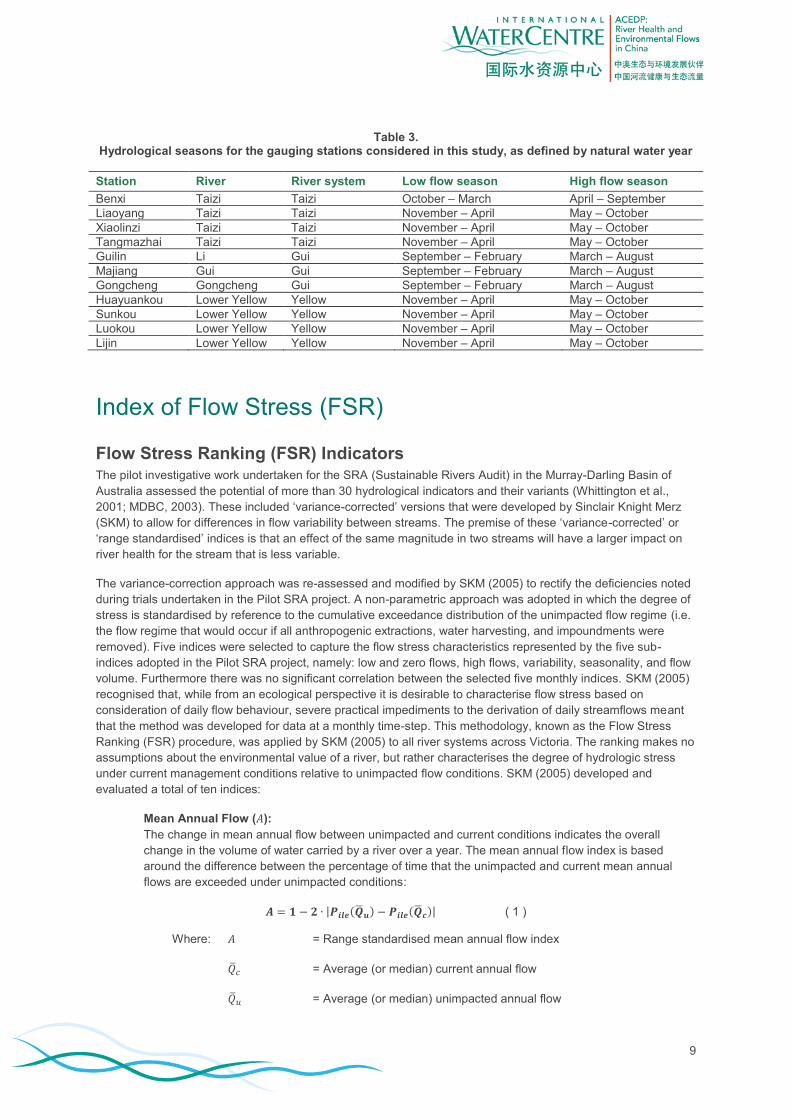
Table 3. Hydrological seasons for the gauging stations considered in this study, as defined by natural water year

Station River River system Low flow season High flow season

Benxi Taizi Taizi October – March April – September

Liaoyang Taizi Taizi November – April May – October

Xiaolinzi Taizi Taizi November – April May – October

Tangmazhai Taizi Taizi November – April May – October

Guilin Li Gui September – February March – August

Majiang Gui Gui September – February March – August

Gongcheng Gongcheng Gui September – February March – August

Huayuankou Lower Yellow Yellow November – April May – October

Sunkou Lower Yellow Yellow November – April May – October

Luokou Lower Yellow Yellow November – April May – October

Lijin Lower Yellow Yellow November – April May – October

Index of Flow Stress (FSR)

Flow Stress Ranking (FSR) Indicators The pilot investigative work undertaken for the SRA (Sustainable Rivers Audit) in the Murray-Darling Basin of

Australia assessed the potential of more than 30 hydrological indicators and their variants (Whittington et al.,

2001; MDBC, 2003). These included ‘variance-corrected’ versions that were developed by Sinclair Knight Merz

(SKM) to allow for differences in flow variability between streams. The premise of these ‘variance-corrected’ or

‘range standardised’ indices is that an effect of the same magnitude in two streams will have a larger impact on

river health for the stream that is less variable.

The variance-correction approach was re-assessed and modified by SKM (2005) to rectify the deficiencies noted

during trials undertaken in the Pilot SRA project. A non-parametric approach was adopted in which the degree of

stress is standardised by reference to the cumulative exceedance distribution of the unimpacted flow regime (i.e.

the flow regime that would occur if all anthropogenic extractions, water harvesting, and impoundments were

removed). Five indices were selected to capture the flow stress characteristics represented by the five sub-

indices adopted in the Pilot SRA project, namely: low and zero flows, high flows, variability, seasonality, and flow

volume. Furthermore there was no significant correlation between the selected five monthly indices. SKM (2005)

recognised that, while from an ecological perspective it is desirable to characterise flow stress based on

consideration of daily flow behaviour, severe practical impediments to the derivation of daily streamflows meant

that the method was developed for data at a monthly time-step. This methodology, known as the Flow Stress

Ranking (FSR) procedure, was applied by SKM (2005) to all river systems across Victoria. The ranking makes no

assumptions about the environmental value of a river, but rather characterises the degree of hydrologic stress

under current management conditions relative to unimpacted flow conditions. SKM (2005) developed and

evaluated a total of ten indices:

Mean Annual Flow ( ):

The change in mean annual flow between unimpacted and current conditions indicates the overall

change in the volume of water carried by a river over a year. The mean annual flow index is based

around the difference between the percentage of time that the unimpacted and current mean annual

flows are exceeded under unimpacted conditions:

( 1 )

Where: = Range standardised mean annual flow index

= Average (or median) current annual flow

= Average (or median) unimpacted annual flow

10

= Proportion of time that the average (or median) current annual flow is

exceeded under unimpacted conditions

= Proportion of time that the average (or median) unimpacted annual

flow is exceeded under unimpacted conditions

In order to make the index more ecologically significant, the Eqn 1 was applied by SKM (2005) to five

flow values, ranging from 80% to 120% of the mean. The mean annual flow index was calculated as the

average of the range-standardised indices for the five flow intervals.

Seasonal Amplitude ( ):

The seasonal amplitude index compares the difference in magnitude between the high and low flows

within each year under current and unimpacted conditions. The index reflects changes to seasonal

variability in in-stream hydraulics and depth of flooding. The index is calculated using the difference

between the percentage of years that the unimpacted and current seasonal amplitudes are exceeded

under unimpacted conditions.

( 2 )

Where: = Range standardised seasonal amplitude index

= Average current seasonal amplitude

= Average unimpacted seasonal amplitude

= Proportion of time that the average current seasonal amplitude is


= Proportion of time that the average unimpacted seasonal amplitude is


Seasonal Period ( ):

The timing of periods of flooding and low flows has an important influence on how floodplain and riverine

ecosystems respond (SKM, 2005), and this index provides a measure of the shift in the timing of the

maximum flow month and the minimum flow month under both unimpacted and current conditions. The

index is based on frequency distributions that reflect the percentage of years that peak and minimum

annual flows fall within each given month under current and unimpacted conditions:

( 3 )

Where: = Comparison of frequency distribution seasonal period index

= The percentage of years the th

month has the peak annual flow under

current conditions


month has the peak annual flow under

unimpacted conditions


month has the minimum annual flow

under current conditions


month has the minimum annual flow

under unimpacted conditions

Low Flow Magnitude ( ):

Altering the magnitude of low flows changes the availability of instream habitat, which can lead to a long

term reduction in the viability of populations of flora and fauna (SKM, 2005). The index measures the

change in low flow magnitude under current and unimpacted conditions. Review of previous studies by

11

SKM (2005) showed that low flow requirements often correspond to the daily 90% exceedance flow,

though as a monthly time step is used the index is calculated using two flow thresholds: one based on

the flow exceeded 91.7% of the time (i.e. 11 months out of 12) and the other based on the flow

exceeded 83.3% of the time (10 months out of 12):

( 4 )

Where: = Range standardised low flow index based on the 91.7% exceedance

flow

= Current 91.7% exceedance flow

= Unimpacted 91.7% exceedance flow

= Proportion of time that the current 91.7% exceedance flow is

exceeded by the unimpacted 91.7% exceedance flow

= Proportion of time that the unimpacted 91.7% exceedance flow is


The low flow index is calculated as the average of the variance corrected low flow index based on the

91.7% exceedance flow and the variance corrected low flow index based on the 83.3% exceedance flow:

( 5 )

Where: = Range standardised low flow index

= Range standardised low flow index based on the 91.7% exceedance

flow


flow

High Flow Magnitude ( ):

High flows act as a natural disturbance in river systems, removing vegetation and organic matter and

resetting successional processes (SKM, 2005). This index measures the change in high flows under

current and unimpacted conditions. The approach adopted by SKM (2005) was to calculate the high flow

index is similar to that used to calculate the low flow index. The monthly high flow index is calculated

based on the 8.3% and 16.7% exceedance flows. Two intervals were used to cover a range of high

flows rather than basing the index on a single value.

( 6 )

Where: = Range standardised low flow index based on the 8.3% exceedance

flow

= Current 8.3% exceedance flow

= Unimpacted 8.3% exceedance flow

= Proportion of time that the current 8.37% exceedance flow is


= Proportion of time that the unimpacted 8.3% exceedance flow is


The low flow index is calculated as the average of the variance corrected low flow index based on the

8.3% exceedance flow and the variance corrected low flow index based on the 16.7% exceedance flow:

12

( 7 )

Where: = Range standardised low flow index


flow


flow

Low Flow Spells ( ):

The low flow index mentioned above is based solely on flow magnitude and does not consider the

variations in duration that a stream may spend below a given threshold. Information on the frequency

and duration of low flows provides a direct indication of the availability of aquatic habitat during low flow

periods, which can impact on the ability of river systems to sustain plant and animal populations (SKM,

2005). The index is calculated from a partial series frequency analysis of the duration of spells above

two thresholds corresponding to flows exceeded 83.3% and 91.7% of the time (these percentiles

correspond to the rank of the lowest two months in a calendar year).

High Flow Spells ( ):

In a similar fashion to low flow spells, the high flow spells index is based on analysing differences in the

frequency and duration of high flow spells above selected thresholds. The duration of the spell events

for flows exceeded 8.3% and 16.7% of the time (which correspond to the first and second highest

monthly flows in each year) are determined for both current and unimpacted conditions, and a partial

series analysis is used to characterise differences in the duration and frequency of the events.

Proportion of Zero Flows ( ):

Periods of zero flow are a natural feature of ephemeral rivers and creeks, however increases in the

natural duration of cease to flow periods are regarded as harmful to aquatic ecosystems (SKM, 2005).

The proportion of zero flow index simply reflects the differences in the proportion of zero flow occurring

under unimpacted and current conditions. In the FSR, zero flow is defined as the flow exceeded 99.5%

of the time (i.e. not cease to flow), in an attempt to lessen the problem of streamflow gauges being

unreliable at very low flow levels.

( 8 )

Where: = Proportion of zero flow (flow exceeded 99.5% of the time) index

= Proportion of zero flow (flow exceeded 99.5% of the time) over the

whole record under unimpacted conditions

= Proportion of zero flow (flow exceeded 99.5% of the time) over the

whole record under current conditions

Flow Duration Curve ( ):

The flow duration curve provides an efficient summary of the overall nature of the flow regime. It does

not characterise any particular component of the flow regime, nor does it include any description of flow

sequencing, and it is therefore difficult to identify any specific ecological effects (SKM, 2005). The flow

duration index compares changes in the shape of the non-zero part of the flow duration curve under

unimpacted and current conditions. This indicator tends to characterise mid-magnitude flows, as the

extremes of the flow duration curve are not considered as part of the index calculation:

( 9 )

Where: = Flow duration index

= Flow under unimpacted conditions (at 10 equal log intervals)

13

= Proportion of time that the flow is exceeded under unimpacted

conditions

= Flow under current conditions that has an exceedance percentile

equal to

= Proportion of time that the flow is exceeded under unimpacted

conditions

Flow Variability ( ):

This index is similar to the seasonal amplitude index in that it reflects variability over a year. The key

difference is that the variation index measures variability across all months rather than simply the

difference between minimum and maximum monthly flows (SKM, 2005). The index simply compares the

coefficient of variation of monthly flows between current and unimpacted conditions:

( 10 )

1

Where: = Index of monthly variability

= Current monthly coefficient of variation

= Unimpacted monthly coefficient of variation

The derivation of the and requires curve fitting, which involves a subjective element. For this reason

these indicators were not considered in this application to the Taizi and Gui rivers. Based on extensive analysis

of streamflow data from Victoria, SKM (2005) narrowed down their list of indicators to five that were not

correlated with each other (they also excluded and ). Such testing of the indicators has not been

undertaken for Chinese rivers, so for this study, indicators cannot be excluded on those grounds. The SRA

(Davies et al., 2010) included two additional indicators:

Mean Annual Discharge ( )

This index is simply the ratio of the mean annual discharge in the current discharge series divided by the

mean annual discharge in the unimpacted series.

Median Annual Discharge ( )

This index is simply the ratio of the median (50th

percentile) annual discharge in the current discharge

series divided by the median annual discharge in the unimpacted series.

After excluding and , and including and , ten indicators remained. The FSR procedure also

calculates a combined indicator score, which is simply the average of , , , and

(SKM, 2005). Here, the combined indicator score was denoted as .

Application of the FSR to Chinese case studies

Calculation procedure

Prior to calculating the FSR scores, it is necessary to decide on the water year. The SKM FSR program

automatically selects the water year, but on the basis of an assumption that did not suit the seasonality of

Chinese rivers. The water year was determined using the method based on the lowest six-month sum of median

monthly flows (Figure 5, Table 3).

In Australia, the FSR is applied to modelled monthly stream flow data, comparing the current and reference

series. In China, modelled current series are not available, and modelled reference series are not commonly

1 The original formula for CV in SKM (2005) was

, which would give a value >1 if CV declined with regulation

(which is the most common impact of regulation on flow variability). Inverting this equation would not solve the problem of values potentially exceeding 1, so it was modified here to always give a value between zero and 1.

14

available (Table 1). Modelled monthly reference data (Figure 4) were not available for the Taizi River (Table 1). In

this case, the FSR was computed on the basis of comparing the statistics calculated for the pre-dam period, with

one (for Benxi) or two (the other stations) post-dam periods. The gauged historical flow time series (Figure 4)

were divided into pre-dam and post-dam periods (Table 2):

Pre-Tanghe/Shenwo: Pre-1969

Post-Tanghe/Shenwo: 1973 - 1994

Post-Guanyinge: 1996 - 2007

Comparing data from different periods of time is a departure from the original FSR method as described by SKM

(2005), and the effect of using different length time series on the FSR procedure is not known. However, it is

certain that non-stationarity in the data due to climate change or land use change would affect the result (i.e.

confound the dam effect). Without modelled natural flow data it is not possible to separate the impacts of climate

change and water resources development on hydrological indices. The Mann-Kendall test was applied to the

Taizi River historical annual flow data and there was no evidence of significant trend. This does not discount the

possibility that there is a climate change signal in the hydrology data, merely establishing that such a signal is not

apparent at the scale of annual flows.

Modelled reference flow time series (Figure 4) data were available for the Gui and Yellow rivers (Table 1).

Modelled current flow time series (Figure 4) were not available, so the gauged historical flow series (Figure 4)

were compared with the reference flow series. This is problematic because at the beginning of the time series the

regulation effect is negligible; the effect increases with time, and is at its maximum at the end of the time series

(Figure 4). The FSR calculation integrates this increasing effect over time, such that the indicator scores

underestimate the degree of flow stress under the current level of water resources development. The issues with

climate change and land-use change mentioned above in connection with the Tiazi River data are also relevant

to the Gui and Yellow river data.

A program was prepared in Microsoft ExcelTM

to undertake the FSR calculations. The results were verified by

calculating the FSR indicators using the FSR computer program supplied for that purpose by SKM (Rory Nathan,

SKM, pers. comm., 2010). The main reason for performing the calculation in MS ExcelTM

was that the SKM FSR

program only calculated the final five indicators selected for use in Victoria.

In applying the FSR to the Chinese case studies, there were instances of negative FSR scores or scores

exceeding 1 (the scores should lie between 0 and 1). This occurred in cases of extreme flow deviation, or where

the flow index was higher in the current series, compared to the unimpaired series. In the case of a negative

score, a score of zero was assigned, and in the case of a score greater than 1, a score of 1 was assigned.

FSR application to the Taizi River Application of the FSR to the Taizi River data produced mixed results (Figure 6, Figure 7, Figure 8 and Figure 9).

For annual flow indicators, always gave a lower score than , and always gave a lower score than .

There is clearly redundancy in these indicators. Of the three, was the most sensitive to hydrological change,

but perhaps too sensitive, as a score of 0.06 was scored at Liaoyang, and in China there are rivers with much

greater reduction in annual flow than the Taizi.

Seasonal amplitude ( ) was not a useful indicator, as it consistently scored low, and the Taizi River still

maintains a reasonable seasonal difference in flows (Figure 63). Also, the measure of seasonal amplitude is to

some extent expressed in the low flow and high flow indicators.

Seasonal periodicity ( ) measures shift in seasonality. The Taizi River has altered seasonality of flows (Figure

63), which is captured by this indicator.

The low flow ( ) and high flow ( ) indicators were very sensitive, particularly , which

scored very low in most cases, except for Tangmazhai station. The higher value for Tangmazhai station was

logical, as regulation had less effect on low flows at that station. The values scored for the Taizi River

appear to cover a great range, perhaps greater than would be expected for this indicator to be applicable over all

the rivers of China. scores were more consistent between the stations. A problem for interpretation is

15

that the low flow and high flow indicators show a value less than 1 if these indicators are different in the current

hydrology compared to the unimpaired hydrology. In most cases, a decrease would be of more concern than an

increase, but there is no indication in the index values whether the flows increased or decreased with regulation.

was sensitive to changes in very low flow, showing a lower value for Liaoyang station where frequency

of cease to flow events increased after regulation.

was not a sensitive indicator, largely because it responds to changes in the mid-range flows, which tend not

to be affected by regulation to the same relative degree as flood flows and low flows.

showed fairly consistent results across the Taizi River stations. This indicator may lack sensitivity as a river

health indicator. Also, the index value does not indicate if flows have become more or less variable with

regulation.

The averaged score, , was not particularly useful for interpreting flow issues, as it combined indicators that

scored low with those that scored high. So, all stations received a mid-range flow stress score. The score

indicated higher flow stress at gauges close to the dams, with natural inflows ameliorating the impact further

downstream. However, perhaps unrealistically, the score indicated that the impact of three upstream dams

(Tangehe, Shenwo and Guanyinge) on hydrology at Liaoyang was similar to the impact of one dam (Guanyinge)

at Benxi.

Figure 6. Results of FSR calculation for Benxi station, comparing pre-Guanyinge with post-Guanyinge data. Indicator codes explained in the text.

0.59

0.10

0.35

0.18

0.47

0.99

0.85

0.683 0.67

0.75

0.53

0.0

0.1

0.2

0.3

0.4

0.5

0.6

0.7

0.8

0.9

1.0

Hyd

rolo

gic

al c

han

ge In

dex v

alu

e

Benxi (pre-Guanyinge V. post-Guanyinge)

16

Figure 7. Results of FSR calculation for Liaoyang station, comparing pre-Tanghe/Shenwo with post-Tanghe/Shenwo data (top) and pre-Tanghe/Shenwo with post-Guanyinge data. Indicator codes explained

in the text.

0.23

0.13

0.60

0.00

0.77

0.60

0.87

0.980

0.73

0.550.59

0.0

0.1

0.2

0.3

0.4

0.5

0.6

0.7

0.8

0.9

1.0

Hyd

rolo

gic

al ch

an

ge In

dex v

alu

e

Liaoyang (pre-Tanghe/Shenwo V. post-Tanghe/Shenwo)

0.06 0.09

0.32

0.00

0.68

0.770.84

0.912

0.54

0.44

0.54

0.0

0.1

0.2

0.3

0.4

0.5

0.6

0.7

0.8

0.9

1.0

Hyd

rolo

gic

al c

han

ge In

dex v

alu

e

Liaoyang (pre-Tanghe/Shenwo V. post-Guanyinge)

17

Figure 8. Results of FSR calculation for Xiaolinzi station, comparing pre-Tanghe/Shenwo with post-Tanghe/Shenwo data (top) and pre-Tanghe/Shenwo with post-Guanyinge data. Indicator codes explained

in the text.

0.34

0.13

0.67

0.03

0.740.79

0.920.991

0.78

0.62 0.64

0.0

0.1

0.2

0.3

0.4

0.5

0.6

0.7

0.8

0.9

1.0

Hyd

rolo

gic

al ch

an

ge In

dex v

alu

e

Xiaolinzi (pre-Tanghe/Shenwo V. post-Tanghe/Shenwo)

0.10 0.03

0.46

0.34

0.66

0.860.90

0.937

0.58

0.48

0.65

0.0

0.1

0.2

0.3

0.4

0.5

0.6

0.7

0.8

0.9

1.0

Hyd

rolo

gic

al ch

an

ge In

dex v

alu

e

Xiaolinzi (pre-Tanghe/Shenwo V. post-Guanyinge)

18

Figure 9. Results of FSR calculation for Tangmazhai station, comparing pre-Tanghe/Shenwo with post-Tanghe/Shenwo data (top) and pre-Tanghe/Shenwo with post-Guanyinge data. Indicator codes explained

in the text.

FSR application to the Gui River The Qingshitan dam, operational from 1964, has a fairly small catchment area and would not be expected to

have a major impact on the hydrology of the Li and Gui Rivers. The rivers of the catchment have also been

subjected to water abstraction. For this river system, the FSR indicators were calculated over the entire period of

historical record (1956 – 2010) using the modelled natural flows over the period 1956 – 2000 as the reference.

Application of the FSR to the Gui River data suggested a low degree of flow alteration in this system (Figure 10).

Because the FSR scores were all close to 1, they revealed very little about the way regulation has affected the

river. There were no differences between the FSR scores of the three stations that could be interpreted in terms

of different regulation impacts.

0.38

0.12

0.60

0.96

0.72

0.97 0.95 0.935

0.84

0.67

0.84

0.0

0.1

0.2

0.3

0.4

0.5

0.6

0.7

0.8

0.9

1.0

Hyd

rolo

gic

al ch

an

ge In

dex v

alu

e

Tangmazhai (pre-Tanghe/Shenwo V. post-Tanghe/Shenwo)

0.15 0.00

0.42

0.56

0.65

0.990.96

0.887

0.64

0.54

0.70

0.0

0.1

0.2

0.3

0.4

0.5

0.6

0.7

0.8

0.9

1.0

Hyd

rolo

gic

al c

han

ge In

dex v

alu

e

Tangmazhai (pre-Tanghe/Shenwo V. post-Guanyinge)

19

Figure 10. Results of FSR calculation for three Gui River system stations, comparing modelled reference data (1956 – 2000) with historical gauged data (1956 – 2010). Indicator codes explained in the text.

0.770.82

0.93 0.92 0.90

0.99 0.97 1.00

0.86

0.990.95

0.0

0.1

0.2

0.3

0.4

0.5

0.6

0.7

0.8

0.9

1.0

Hyd

rolo

gic

al c

han

ge In

dex v

alu

e

Guilin

0.820.86

0.920.86 0.84

1.000.97 0.98

0.94 0.95 0.92

0.0

0.1

0.2

0.3

0.4

0.5

0.6

0.7

0.8

0.9

1.0

Hyd

rolo

gic

al c

han

ge In

dex v

alu

e

Majiang/Jingnan

0.90

0.980.94

0.85

0.951.00 0.97 0.98 0.96 0.97 0.94

0.0

0.1

0.2

0.3

0.4

0.5

0.6

0.7

0.8

0.9

1.0

Hyd

rolo

gic

al c

han

ge In

dex v

alu

e

Gongcheng

20

FSR application to the Yellow River The hydrology of the lower Yellow River has been impacted by construction of many dams and by water

abstraction. The first major dam to directly impact the lower river was Sanmenxia, operational since 1961. The

next major dam was Longyangxia, operational since 1987, and then Xiaolangdi, operational since 2000. The FSR

indicators were calculated for these three main periods of regulation, using paired reference and historical data

from Huayuankou and Lijin gauging stations. The lower Yellow River was impacted by regulation prior to

operation of Sanmenxia dam, but the period of record before 1961 was too short to generate reliable statistics.

Application of the FSR to the Yellow River data suggested a high degree of flow alteration in this system (Figure

11 and Figure 12). Lijin was impacted to a greater degree than Huayuankou, because a significant volume of

water is diverted from the river between Huayuankou and Lijin for irrigation. The FSR indicator scores tended to

decrease as each dam became operational. The operation of Xiaolangdi dam did not lead to any significant

improvements in FSR indicator scores, despite introduction of the water and sediment discharge regulation

(WSDR) system in this period.

Discussion of FSR indicators The FSR scores showed some promise as meaningful indicators of hydrological change. The indicators

characterised the aspects of the flow regime normally considered to be important for ecological river health (Poff

et al., 1997). It is not possible to eliminate any of these indicators on the basis of this limited application. However,

it appears that some indicators may be more useful than others, and some will be correlated. Perhaps the least

useful indicators were , , , and , and interestingly, all but were not included in application of the

FSR procedure in Victoria (SKM, 2005). Because is calculated on the entire time series, it is likely to be

sensitive only to very major flow changes that cause the flow to become relatively constant. In most regulated

rivers the flow is not constant, as water demands (and thus supply) are variable, seasonally and from year to year.

The only station to show low scores for was Lijin on the Lower yellow River.

A limitation of the FSR is that changes in the flow indicators associated with regulation are treated equally,

whether they increase or decrease. The ecological implications of a decrease are likely to be different (i.e. usually

more serious) than those of an increase. One way to manage this would be to modify the FSR formulas to weight

decreases higher than increases.

Application of the FSR to the Gui River suggested a low level of flow regulation in this catchment. During this

period the Qingshitan dam began operation, in 1964, but this dam is located on a relatively small tributary, and in

the context of the characteristically high runoff of the Gui River system, it would not be expected to have a major

impact on flows at Guilin, and especially at Majiang/Jingnan. The other flow regulation effect was a gradual

increase in water diversions from the river over time, which applied in particular to Majiang/Jingnan and

Gongcheng gauges. This is known from water use figures, but is not revealed by the FSR approach. The method

of comparison of historical flows with modelled reference flows is not ideal, because it averages the degree of

regulation over time, such that the FSR result does not properly reflect the current degree of regulation.

While the FSR indicators satisfactorily measured degrees of flow stress between monthly flow time series with

different levels of water resources development, the FSR approach is not useful as an annual reporting tool,

unless using fully modelled reference and current flow data and where the current model conditions are updated

and re-run annually. This is a very large undertaking, and is one reason why the SRA intends to only report the

flow stress indicators every three years (Davies et al., 2008).

21

Figure 11. Results of FSR calculation for Huayuankou station (lower Yellow River), comparing modelled reference data with historical gauged data for three periods: post-Sanmenxia (1961-1985), post-Longyangxia (1987-1998) and post-Xiaolangdi (2000-2008). Indicator codes explained in the text.

0.30

0.65

0.56

0.430.38

0.900.85 0.88

0.74 0.75

0.63

0.0

0.1

0.2

0.3

0.4

0.5

0.6

0.7

0.8

0.9

1.0

Hyd

rolo

gic

al c

han

ge In

dex v

alu

e

Huayuankou (post-Sanmenxia)

0.36

0.07

0.640.58

0.18

0.960.91

0.99

0.60 0.610.67

0.0

0.1

0.2

0.3

0.4

0.5

0.6

0.7

0.8

0.9

1.0

Hyd

rolo

gic

al c

han

ge In

dex v

alu

e

Huayuankou (post-Longyangxia)

0.24

0.00

0.44

0.02 0.10

0.90 0.870.92

0.56 0.57

0.47

0.0

0.1

0.2

0.3

0.4

0.5

0.6

0.7

0.8

0.9

1.0

Hyd

rolo

gic

al c

han

ge In

dex v

alu

e

Huayuankou (post-Xiaolangdi)

22

Figure 12. Results of FSR calculation for Lijin station (lower Yellow River), comparing modelled reference data with historical gauged data for three periods: post-Sanmenxia (1961-1985), post-Longyangxia (1987-

1998) and post-Xiaolangdi (2000-2008). Indicator codes explained in the text.

0.25

0.630.59

0.00

0.37

0.710.79

0.74

0.640.58

0.48

0.0

0.1

0.2

0.3

0.4

0.5

0.6

0.7

0.8

0.9

1.0

Hyd

rolo

gic

al c

han

ge In

dex v

alu

e

Lijin (post-Sanmenxia)

0.28

0.10

0.41

0.000.20

0.34

0.88

0.57

0.34 0.340.30

0.0

0.1

0.2

0.3

0.4

0.5

0.6

0.7

0.8

0.9

1.0

Hyd

rolo

gic

al c

han

ge In

dex v

alu

e

Lijin (post-Longyangxia)

0.18

0.41 0.43

0.01 0.16 0.12

0.82

0.65

0.36

0.46

0.27

0.0

0.1

0.2

0.3

0.4

0.5

0.6

0.7

0.8

0.9

1.0

Hyd

rolo

gic

al c

han

ge In

dex v

alu

e

Lijin (post-Xiaolangdi)

23

Chinese Hydrology and Water Resources Index (HD)

Introduction In China, a simple method of measuring flow alteration that is based on comparing the flows in any month with

the typical flows for that month prior to regulation of the river would have natural appeal. This is because:

Hydrological data are often available only as historical monthly flow series.

The Tennant method (or variants of the seasonal hydrological factoring method that uses monthly flow

data) is popular as a method of assessing environmental flow needs (Wang et al., 2009). This method

could be applied in reverse to provide an indicator of hydrological health, whereby the current flow

regime is compared against the Tennant method ecological health standards.

The National Technical Working Group for the Health Assessment of Rivers and Lakes, Department of Water

Resources Management, Ministry of Water Resources People’s Republic of China, developed indicators,

standards and methods for a nation-wide river health assessment program, currently being tested in a number of

pilot rivers and lakes (NTWGHARL, 2010). The approach included a hydrology indicator, called Hydrology and

Water Resources (Hydrology, HD) (Table 4).

Table 4. Hydrology and water resources index and indicators proposed pilot testing by the China nation-wide

river health assessment program. Source: NTWGHARL (2010).

Criteria layer River indicator layer Code Indicators Index

Hydrology and water resources Flow variation degree FD FDr

HDr Satisfaction level of ecological flow EF EF1r, EF2r

The “satisfaction level of ecological flow” (EF) indicators are based on the Tennant method. Some concerns have

been expressed in the literature about the Tennant method:

The method may have limited transferability beyond the Montana, Nebraska and Wyoming streams

used by Tennant (1976) to develop the method (for example, see Gordon et al., 2004; Mann, 2006). For

example, Tennant (1976) showed that 30% of the mean annual flow (MAF) or higher provided depths of

0.45 – 0.60 m and velocities of 0.45 – 0.60 m/s, which were considered suitable for the organisms in the

surveyed streams. However, it is clear from this information that the streams surveyed by Tennant (1976)

were small, and these relationships may not apply in bigger rivers, or in streams of significantly different

hydrological, geomorphological or ecological character.

The method essentially recommends only two baseflow levels, one for the low flow and one for the high

flow season, plus a single high flow pulse (which is usually ignored in Chinese applications of the

Tennant method). Thus, the method does not address the dynamic and variable nature of a natural

hydrological regime (King et al., 1999).

The “flow variation degree” (FD) indicator requires availability of modelled natural flow data for the corresponding

time period over which modelled current or historical gauged flow data are available. In China, such modelled

natural flow data are available only for certain key hydrology stations, and even then, only for a particular time

period, usually 1956 – 2000. Modelling natural flow is not a trivial task, so models are usually updated only

periodically, not annually. Thus, while it is technically possible to calculate a FD score for any particular year, it

would not normally be possible to calculate the score for a recent year to include in a current river health report

hard.

The above limitations suggest that there may be situations in China where the proposed hydrology index for

assessment of river health will not be appropriate. This report reviews the general applicability of the HD index

using the Taizi and Gui rivers as examples.

24

Methodology

Flow variation degree (FD) The method for calculation of the HD was set out in (NTWGHARL, 2010). The degree of flow rate variation (FD)

is based on the Amended Annual Proportion of Flow Deviation indicator (AAPFD), first proposed by Gehrke et al.

(1995) as the APFD and later amended for use as the initial hydrology indicator in the Index of Stream Condition

(ISC) in Victoria, Australia (Ladson and White, 1999; Ladson et al., 1999). The ISC later adopted the FSR as the

hydrological index. Calculation of the AAPFD (or FD) requires availability of two modelled monthly time series:

the flow assuming current levels of water resources development (current), and the flow assuming no water

resources development (reference) (Figure 4).

Gehrke et al. (1995) found that the APFD was correlated with fish species diversity, but no such correlation has

been reported for the AAPFD. The AAPFD is the sum of the ratio of change in flow in each month (current –

reference) to average long term reference flow for each month:

( 11 )

where,

= number of years in modelled period

= modelled current flow for month in year

= modelled reference flow for month in year

= mean reference flow for month across years

The original APFD used reference monthly flow ( ) as the denominator, but this was problematic for

ephemeral streams where flow can cease in some months. The AAPFD score is calculated for each month and

each year of modelled data, and the mean AAPFD over the modelled period is the characteristic score for the

station. Higher values of AAPDF indicate a greater degree of hydrological alteration. For a range of regulated

New South Wales and Victorian streams examined by Ladson and White (1999, p. 22), the highest AAPFD score

was 5, while the lowest rating was 0.24. For use in the ISC, the raw AAPFD index value was converted to a rating

in the range 0 – 10, with lower values indicating greater flow alteration (Figure 13). Intermediate AAPFD values

were interpolated between the two corresponding ratings.

In the Chinese application of the AAPFD, the FD score is calculated (assessed) for each year rather than over a

period of time. There is one other important difference in FD compared to AAPFD. In the formula for the FD, the

denominator is the mean monthly reference discharge over the year being assessed, while in the formula for the

AAPFD the denominator is the mean monthly reference discharge over the entire modelled period, and is specific

to each month (in the APFD it is the reference flow for the month of the year being assessed). The rationale

behind this alteration of the AAPFD formula for the Chinese application is unknown. The formula for FD for any

assessed year is:

( 12 )

where,

= gauged historical flow for month of the assessed year

= modelled reference flow for month of the assessed year

25

Like the AAPFD, the raw FD score is converted to a rating (FDr), which in this case is in the range 0 – 100, with

lower values indicating greater flow alteration. The FD conversion gives a lower rating than that of the AAPFD for

the same raw score (Figure 13).

Figure 13. Relationships for converting the FD and the AAPFD scores to a rating. The AAPFD ratings are actually over the scale 0 – 10, but here the scale of 0 – 100 was used.

Satisfaction level of ecological flow (EF) According to NTWGHARL (2010), EF should be calculated using daily flow data, but the calculation could also be

made using monthly flow data. There are two values of EF, one for the low flow season, given as April to

September, and one for the high flow season, given as October to March, which happen to be the same seasonal

definitions used by Tennant (1976). The value of EF is the lowest value of the ratio of the daily flow divided by the

mean annual flow (MAF), expressed as a daily flow, calculated over a long period. In the Tennant method, the

MAF is calculated over a period of time when flow was unregulated. The Chinese method requires that MAF be

calculated over a period of at least 30 years, but does not specify whether this period should represent

unregulated conditions. The requirement of 30 years of data means that in many places flow records would have

to be available as far back as the early-1950s if the period was to represent unregulated conditions (as dam

construction began in earnest in the 1980s).

The formulas for EF are:

( 13 )

where,

= is the gauged historical daily flow in the assessed year

= mean annual flow (MAF), expressed as a daily flow, calculated over a long period

The EF scores are converted to a rating based on the regimens recommended by Tennant (1976) for streams he

surveyed in Wyoming, Nebraska and Montana (Table 5). The EFr score is the smallest score of EF1r and EF2r.

0

10

20

30

40

50

60

70

80

90

100

0 1 2 3 4 5 6

Flo

w d

evia

tio

n r

ati

ng

Flow deviation score

AAPFD

FD

26

Table 5. Standards for assessing the EF scores. Source: NTWGHARL (2010). The qualitative descriptions were

taken from Tennant (1976).

Grade Qualitative description such as habitat

Recommended regimens (percentage of annual mean flow)

Rating (EF1r and

EF2r) EF1: ordinary

water period (Oct – Mar) EF2: spawning and nursing

period of fish (Apr – Sep)

1 Flushing or maximum 200% 200% 100

2 Optimum range 60 – 100% 60 – 100% 100

3 Outstanding 40% 60% 100

4 Excellent 30% 50% 100

5 Good 20% 40% 80

6 Fair or degrading 10% 30% 40

7 Poor or minimum 10% 10% 20

8 Severe degradation < 10% < 10% 0

The final rating value of HDr is the weighted sum of FDr and EFr:

( 14 )

where,

= a weighting, suggested to be 0.3

= a weighting, suggested to be 0.7

Constraints on application of HD

Application of the HD method is restricted to situations where:

A modelled reference monthly flow series is available (for FD calculation)

A long-term historical daily flow series is available (for EF calculation)

This limits the method to gauges where reference flows have been modelled, and presumes that daily flow

records are readily available. In reality, long-term daily flow records can be difficult to obtain, and any modelled

reference flow data is unlikely to be current. To test the method, FD was calculated for selected gauges on the

Gui and lower Yellow rivers, where modelled reference flows were available, and EF was calculated for selected

gauges on the Taizi and lower Yellow rivers, where long-term daily flow records were available. As monthly flows

are more likely to be available in China, the EF calculation was also made using monthly data.

It would be possible to calculate FD using only historical flow data, by calculating from a pre-regulation period

of historical record, and then substituting for in Eqn 12. However, this would result in high values of FD

raw score, as, in any month, the deviation of actual flow from the mean pre-regulation flow would generally be

much greater than the deviation from the reference flow for that month. For this reason, FD was only calculated

using the modelled reference flow data from the Gui River system and Lower Yellow River stations.

Definition of water year and seasons NTWGHARL (2010) does not mention whether the FD and EF indicator values should be calculated over the

calendar year or the water year. While the calendar year would usually be assumed as the default, here the

indicators were calculated on the basis of water year (Figure 5 and Table 3) to allow correlation with other

hydrological indicators that were calculated using water year.

The EF method assumes that the seasonality of rivers is constant all over China, and that the seasonality is the

same as that of the Wyoming, Nebraska and Montana rivers studied by Tennant. The biota of a river adapts to

the local hydrological seasonality, so the “spawning and nursing period of fish” (Table 5) would likely show

geographical variation over China. For this application of EF, the EF seasonality was varied according to local

conditions, with EF1 corresponding to the locally defined low flow period and EF2 corresponding to the locally

27

defined high flow period. Because water year was used in the calculation of EF, the low flow period began at the

end of the year before the test year.

Results (FD)

Gui River system

FD scores were calculated for three gauges on the Gui River system for which modelled monthly reference flows

were available. AAPFD scores were calculated for comparison with FD scores to determine the impact of the

alteration of the AAPFD formula by NTWGHARL (2010) to calculate FD. The modelled reference flows were

compared with the historically gauged flows.

The Li River flows from its headwaters through Guilin, Yangshuo and Pingle. In Pingle, the Li River is joined by

the Gongcheng River tributary and it then continues south as the Gui River. The FD score for Guilin station

shows a rise in flow alteration after the Qingshitan dam began operation in 1964. The degree of flow alteration

was slightly elevated through the 1970s, and then lessened (Figure 14). Majiang and Gongcheng stations show a

similar trend of slowly increasing degree of flow alteration (Figure 15 and Figure 16).

Lower Yellow River FD scores were calculated for two gauges on the Lower Yellow River for which modelled monthly reference flows

were available (Figure 17 and Figure 18). AAPFD scores were calculated for comparison with FD scores to

determine the impact of the alteration of the AAPFD formula by NTWGHARL (2010) to calculate FD. The

modelled reference flows were compared with the historically gauged flows.

The FD scores calculated for the Lower Yellow River stations were considerably higher than those for the Gui

River stations. There was a peak in flow diversion in the late-1950s to early-1960s in association with the Great

Leap Forward. FD scores increased noticeably in the mid-1980s in association with operation of Longyangxia

dam (Table 2).

Figure 14. FD and AAPFD raw scores and rating scores for Guilin station on the Li River. The degree of deviation here is small, as the FD score ranges up to 5.

0.0

0.1

0.2

0.3

0.4

0.5

0.6

1957

1958

1959

1960

1961

1962

1963

1964

1965

1966

1967

1968

1969

1970

1971

1972

1973

1974

1975

1976

1977

1978

1979

1980

1981

1982

1983

1984

1985

1986

1987

1988

1989

1990

1991

1992

1993

1994

1995

1996

1997

1998

1999

2000

FD

sco

re

Guilin

FD

AAPFD

0

10

20

30

40

50

60

70

80

90

100

1957

1958

1959

1960

1961

1962

1963

1964

1965

1966

1967

1968

1969

1970

1971

1972

1973

1974

1975

1976

1977

1978

1979

1980

1981

1982

1983

1984

1985

1986

1987

1988

1989

1990

1991

1992

1993

1994

1995

1996

1997

1998

1999

2000

FD

r ra

tin

g

Guilin

FDr

AAPFDr

28

Figure 15. FD and AAPFD raw scores and rating scores for Majiang station on the Gui River. The degree of deviation here is small, as the FD score ranges up to 5.

Figure 16. FD and AAPFD raw scores and rating scores for Gongcheng station on the Gongcheng River. The degree of deviation here is small, as the FD score ranges up to 5.

0.0

0.1

0.2

0.3

0.4

0.5

0.6

1957

1958

1959

1960

1961

1962

1963

1964

1965

1966

1967

1968

1969

1970

1971

1972

1973

1974

1975

1976

1977

1978

1979

1980

1981

1982

1983

1984

1985

1986

1987

1988

1989

1990

1991

1992

1993

1994

1995

1996

1997

1998

1999

2000

FD

sco

re

Majiang

FD

AAPFD

0

10

20

30

40

50

60

70

80

90

100

1957

1958

1959

1960

1961

1962

1963

1964

1965

1966

1967

1968

1969

1970

1971

1972

1973

1974

1975

1976

1977

1978

1979

1980

1981

1982

1983

1984

1985

1986

1987

1988

1989

1990

1991

1992

1993

1994

1995

1996

1997

1998

1999

2000

FD

r ra

tin

g

Majiang

FDr

AAPFDr

0.0

0.1

0.1

0.2

0.2

0.3

0.3

0.4

0.4

0.5

1957

1958

1959

1960

1961

1962

1963

1964

1965

1966

1967

1968

1969

1970

1971

1972

1973

1974

1975

1976

1977

1978

1979

1980

1981

1982

1983

1984

1985

1986

1987

1988

1989

1990

1991

1992

1993

1994

1995

1996

1997

1998

1999

2000

FD

sco

re

Gongcheng

FD

AAPFD

0

10

20

30

40

50

60

70

80

90

100

1957

1958

1959

1960

1961

1962

1963

1964

1965

1966

1967

1968

1969

1970

1971

1972

1973

1974

1975

1976

1977

1978

1979

1980

1981

1982

1983

1984

1985

1986

1987

1988

1989

1990

1991

1992

1993

1994

1995

1996

1997

1998

1999

2000

FD

r ra

tin

g

Gongcheng

FDr

AAPFDr

29

Figure 17. FD and AAPFD raw scores and rating scores for Huayuankou station on the Yellow River.

Figure 18. FD and AAPFD raw scores and rating scores for Lijin station on the Yellow River.

Overall result for FD

On the basis of calculation of the FD indicator for Gui and Lower Yellow River gauges it is apparent that:

0.0

0.5

1.0

1.5

2.0

2.5

3.0

3.5

4.0

1953

1954

1955

1956

1957

1958

1959

1960

1961

1962

1963

1964

1965

1966

1967

1968

1969

1970

1971

1972

1973

1974

1975

1976

1977

1978

1979

1980

1981

1982

1983

1984

1985

1986

1987

1988

1989

1990

1991

1992

1993

1994

1995

1996

1997

1998

1999

2000

2001

2002

2003

2004

2005

2006

2007

2008

FD

sco

re

Huayuankou

FD

AAPFD

0

10

20

30

40

50

60

70

80

90

100

1953

1954

1955

1956

1957

1958

1959

1960

1961

1962

1963

1964

1965

1966

1967

1968

1969

1970

1971

1972

1973

1974

1975

1976

1977

1978

1979

1980

1981

1982

1983

1984

1985

1986

1987

1988

1989

1990

1991

1992

1993

1994

1995

1996

1997

1998

1999

2000

2001

2002

2003

2004

2005

2006

2007

2008

FD

r ra

tin

g

Huayuankou

FDr

AAPFDr

0.0

0.5

1.0

1.5

2.0

2.5

3.0

3.5

4.0

1953

1954

1955

1956

1957

1958

1959

1960

1961

1962

1963

1964

1965

1966

1967

1968

1969

1970

1971

1972

1973

1974

1975

1976

1977

1978

1979

1980

1981

1982

1983

1984

1985

1986

1987

1988

1989

1990

1991

1992

1993

1994

1995

1996

1997

1998

1999

2000

2001

2002

2003

2004

2005

2006

2007

2008

FD

sco

re

Lijin

FD

AAPFD

0

10

20

30

40

50

60

70

80

90

100

1953

1954

1955

1956

1957

1958

1959

1960

1961

1962

1963

1964

1965

1966

1967

1968

1969

1970

1971

1972

1973

1974

1975

1976

1977

1978

1979

1980

1981

1982

1983

1984

1985

1986

1987

1988

1989

1990

1991

1992

1993

1994

1995

1996

1997

1998

1999

2000

2001

2002

2003

2004

2005

2006

2007

2008

FD

r ra

tin

g

Lijin

FDr

AAPFDr

30

The FD raw score is similar to the AAPFD raw score, although the AAPFD raw score is generally lower

and has lower inter-annual variability

The FD rating score is lower than that of the AAPFD, which is largely explained by the more sensitive

relationship used to convert raw scores to rating scores (Figure 13)

The FD score is very sensitive to alteration of overall flow volumes due to flow regulation and water

extraction

Results (EF)

Taizi River

The EF indicator was calculated for four stations on the main stem of the Taizi River (Figure 19 and Figure 20). A

number of observations were made:

The EFr score was governed by EF1r (the score for the low flow period) more often that EF2r

In most years the EFr score calculated from monthly data was higher than that calculated from daily

data

For daily data, the calendar year produced results that were only slightly different to those calculated on

the basis of the water year, but for monthly data (not shown here) the differences were substantial

In most years the EFr score for Taizi River stations was less than “poor or minimum” standard, even in

the pre-dam period

At none of the four Taizi River stations did the EFr scores indicate a reduction in the suitability of flows

for the ecosystem following dam operation. At Benxi gauge the EFr scores actually suggested

significantly improved suitability of flows following construction of Guanyinge dam in 1995.

The reason for the result being more often controlled by EF1r is that the standards for the low flow period are

relatively stricter than those for the high flow period. It is not uncommon for low flow months to contain at least

one day where the flow was less than 20 percent, or even 10 percent of the long-term mean annual flow, even in

the pre-regulation period. These occurrences of relatively low flows, even if brief, control the ultimate result. EFr

scores are higher for monthly flows compared to daily flows, because brief falls in discharge at the daily time-step

are averaged out over the monthly time step. The water year is the more appropriate time standard, but this had

little influence on the overall EFr score.

The Taizi River EFr scores were universally low, even for the unregulated phases of the discharge records. The

apparent “improvement” in the flows at Benxi following the construction of Guanyinge dam can be explained by

use of the river channel to deliver irrigation, industrial and domestic water from the dam to downstream areas,

which increased flows in the low flow period. The flow releases reduced the frequency of low flows with poor

ecosystem suitability (those < 20 percent of mean annual flow), thereby lifting the EFr score. In reality, this form

of flow regulation (increased low flow period flows) could be associated with a negative impact on the ecosystem,

yet the EFr index does not capture this aspect of regulated flow regimes.

Lower Yellow River With respect to EF1r tending to control the result, monthly data producing a higher score than daily data, and

water year producing a similar result to that of calendar year, the Lower Yellow River result was similar to that of

the Gui River system, so those data are not reported here. The Lower Yellow River EFr scores were variable but

generally high prior to Sanmenxia dam. After that, scores were variable from year to year, but low most of the

time, especially at Luokou and Lijin (Figure 21). The operation of Xiaolangdi dam to deliver environmental flows

after 1999 was detectable by EFr, but the rise in the score was relatively small (Figure 21).

31

Figure 19. EFr scores for Benxi and Liaoyang stations on the Taizi River.

0

20

40

60

80

100

1953

1955

1957

1959

1961

1963

1965

1967

1969

1971

1973

1975

1977

1979

1981

1983

1985

1987

1989

1991

1993

1995

1997

1999

2001

2003

2005

2007

EF

r sco

re f

or

wate

r year Benxi

EF1r daily

EF1r monthly

EF2r daily

EF2r monthly

0

20

40

60

80

100

1953

1955

1957

1959

1961

1963

1965

1967

1969

1971

1973

1975

1977

1979

1981

1983

1985

1987

1989

1991

1993

1995

1997

1999

2001

2003

2005

2007

Min

imu

m E

Fr

sco

re

EFr daily (water year)

EFr daily (calendar year)

0

20

40

60

80

100

1953

1955

1957

1959

1961

1963

1965

1967

1969

1971

1973

1975

1977

1979

1981

1983

1985

1987

1989

1991

1993

1995

1997

1999

2001

2003

2005

2007

Min

imu

m E

Fr

sco

re EFr daily (water year)

EFr monthly (water year)

Fair or degrading

Poor or minimum

Dam

0

20

40

60

80

100

1953

1955

1957

1959

1961

1963

1965

1967

1969

1971

1973

1975

1977

1979

1981

1983

1985

1987

1989

1991

1993

1995

1997

1999

2001

2003

2005

2007

EF

r sco

re f

or

wate

r year Liaoyang

EF1r daily

EF1r monthly

EF2r daily

EF2r monthly

0

20

40

60

80

100

1953

1955

1957

1959

1961

1963

1965

1967

1969

1971

1973

1975

1977

1979

1981

1983

1985

1987

1989

1991

1993

1995

1997

1999

2001

2003

2005

2007

Min

imu

m E

Fr

sco

re



0

20

40

60

80

100

1953

1955

1957

1959

1961

1963

1965

1967

1969

1971

1973

1975

1977

1979

1981

1983

1985

1987

1989

1991

1993

1995

1997

1999

2001

2003

2005

2007

Min

imu

m E

Fr

sco



Fair or degrading

Poor or minimum

DamDam Dam

32

Figure 20. EFr scores for Xiaolinzi and Tangmazhai stations on the Taizi River.

0

20

40

60

80

100

1953

1955

1957

1959

1961

1963

1965

1967

1969

1971

1973

1975

1977

1979

1981

1983

1985

1987

1989

1991

1993

1995

1997

1999

2001

2003

2005

2007

EF

r sco

re f

or

wate

r year Xiaolinzi

EF1r daily

EF1r monthly

EF2r daily

EF2r monthly

0

20

40

60

80

100

1953

1955

1957

1959

1961

1963

1965

1967

1969

1971

1973

1975

1977

1979

1981

1983

1985

1987

1989

1991

1993

1995

1997

1999

2001

2003

2005

2007

Min

imu

m E

Fr

sco

re



0

20

40

60

80

100

1953

1955

1957

1959

1961

1963

1965

1967

1969

1971

1973

1975

1977

1979

1981

1983

1985

1987

1989

1991

1993

1995

1997

1999

2001

2003

2005

2007

Min

imu

m E

Fr

sco



Fair or degrading

Poor or minimum

DamDam Dam

0

20

40

60

80

100

1953

1955

1957

1959

1961

1963

1965

1967

1969

1971

1973

1975

1977

1979

1981

1983

1985

1987

1989

1991

1993

1995

1997

1999

2001

2003

2005

2007

EF

r sco

re f

or

wate

r year Tangmazhai

EF1r daily

EF1r monthly

EF2r daily

EF2r monthly

0

20

40

60

80

100

1953

1955

1957

1959

1961

1963

1965

1967

1969

1971

1973

1975

1977

1979

1981

1983

1985

1987

1989

1991

1993

1995

1997

1999

2001

2003

2005

2007

Min

imu

m E

Fr

sco

re



0

20

40

60

80

100

1953

1955

1957

1959

1961

1963

1965

1967

1969

1971

1973

1975

1977

1979

1981

1983

1985

1987

1989

1991

1993

1995

1997

1999

2001

2003

2005

2007

Min

imu

m E

Fr

sco



Fair or degrading

Poor or minimum

DamDam Dam

33

Figure 21. EFr scores for four stations on the Lower Yellow River. Note: start year of time series varies between stations.

Gui River system The EF indicator was calculated for three stations in the Gui River system using monthly data (Figure 22). In this

case, modelled monthly reference data were available, but the time series was limited to 1956 to 2000 (1957 –

2000 when considering water year). Compared to the monthly-derived EFr scores for the Taizi and Lower Yellow

river stations, the EF1r scores in the Gui River tended to be higher, while the EF2r scores were of a similar

magnitude. The Gui River EF1r scores were much more variable from year to year compared with those from the

Taizi and Lower Yellow rivers. As for the Taizi and Lower Yellow river systems, the EFr score was more often

0

20

40

60

80

100

1949

1951

1953

1955

1957

1959

1961

1963

1965

1967

1969

1971

1973

1975

1977

1979

1981

1983

1985

1987

1989

1991

1993

1995

1997

1999

2001

2003

2005

2007

Min

imu

m E

Fr

sco

reHuayuankou


Fair or degrading

Poor or minimum

Dam Dam Dam

0

20

40

60

80

100

1952

1954

1956

1958

1960

1962

1964

1966

1968

1970

1972

1974

1976

1978

1980

1982

1984

1986

1988

1990

1992

1994

1996

1998

2000

2002

2004

2006

2008

Min

imu

m E

Fr

sco

re

Sunkou


Fair or degrading

Poor or minimum

Dam Dam Dam

0

20

40

60

80

100

1949

1951

1953

1955

1957

1959

1961

1963

1965

1967

1969

1971

1973

1975

1977

1979

1981

1983

1985

1987

1989

1991

1993

1995

1997

1999

2001

2003

2005

2007

Min

imu

m E

Fr

sco

re

Luokou


Fair or degrading

Poor or minimum

Dam Dam Dam

0

20

40

60

80

100

1950

1952

1954

1956

1958

1960

1962

1964

1966

1968

1970

1972

1974

1976

1978

1980

1982

1984

1986

1988

1990

1992

1994

1996

1998

2000

2002

2004

2006

2008

Min

imu

m E

Fr

sco

re

Lijin


Fair or degrading

Poor or minimum

Dam Dam Dam

34

controlled by the low flow period EF1r score than the EF2r score. The EFr scores for the Gui River system did not

indicate any impact of regulation on suitability of flows for the ecosystem (Figure 22).

Figure 22. EFr scores for three stations on the Gui River system, calculated from monthly modelled reference and historical gauged data, and using the water year.

Results (HD)

Lower Yellow River

The modelled reference flow data and daily flow data available for Huayuankou and Lijin stations on the Lower

Yellow River allowed calculation of both the EFr and FDr indicators, to give an overall HDr index score (Figure

23). The HDr score was weighted heavily towards the EFr score. The two gauges had very different values of

HDr over time after Sanmenxia dam began operation in 1960 (Figure 23). This is explained by the withdrawal of

irrigation water between Huayuankou and Lijin, which resulted in lower EFr scores and lower FD scores at Lijin.

0

20

40

60

80

100

1957

1959

1961

1963

1965

1967

1969

1971

1973

1975

1977

1979

1981

1983

1985

1987

1989

1991

1993

1995

1997

1999

EF

r sco

re

Guilin

EF1r

EF2r

0

20

40

60

80

100

1957

1959

1961

1963

1965

1967

1969

1971

1973

1975

1977

1979

1981

1983

1985

1987

1989

1991

1993

1995

1997

1999

EF

r sco

re

Majiang

EF1r

EF2r

0

20

40

60

80

100

1957

1959

1961

1963

1965

1967

1969

1971

1973

1975

1977

1979

1981

1983

1985

1987

1989

1991

1993

1995

1997

1999

EF

r sco

re

Gongcheng

EF1r

EF2r

35

Figure 23. HDr scores for two stations on the Lower Yellow River system calculated from monthly modelled reference and historical gauged data, and using the water year. EFr component calculated from

daily data.

Gui River system The modelled reference flow data available for the Gui River system stations allowed calculation of both the EFr

and FDr indicators, to give an overall HDr index score (Figure 24). The HDr score was weighted heavily towards

the EFr score. The three gauges, although located in different parts of the catchment, had similar values of HDr

over time (Figure 24). It is important to recognize that had EFr scores been calculated from daily flow data, rather

than monthly data, the HDr scores would probably have been lower.

Figure 24. HDr scores for three stations on the Gui River system calculated from monthly modelled reference and historical gauged data, and using the water year. EFr component calculated from monthly

data.

Discussion of HD index In general, application of the HD method would be limited to rivers with modelled reference flows, because these

flows are required for calculation of the FD indicator. For these rivers, the time series of HD will be limited by the

length of the period over which reference flows have been simulated, and the time series may not be current (e.g.

the most recent modelled data for the Gui River system are for 2000). Alteration of the AAPFD formula (to give

the FD score) did not have a large effect on the result, but it would be preferable to revert to the original AAPFD

formula so that results can be compared with those from other rivers in the world. Similarly, unless there is a

good reason for altering the relationship to convert the raw FD score to the FD rating score, the original

relationship recommended for the AAPFD should be used. The EF indicator is ideally calculated from a daily flow

series, which is not always readily available in China, further limiting the applicability of the HD index.

0

20

40

60

80

100

1952

1954

1956

1958

1960

1962

1964

1966

1968

1970

1972

1974

1976

1978

1980

1982

1984

1986

1988

1990

1992

1994

1996

1998

2000

2002

2004

2006

2008

HD

r sco

re

Huayuankou

Lijin

0

20

40

60

80

100

1957

1959

1961

1963

1965

1967

1969

1971

1973

1975

1977

1979

1981

1983

1985

1987

1989

1991

1993

1995

1997

1999

HD

r sco

re

Guilin

Majiang

Gongcheng

36

In an unregulated river, the frequency of flows falling into the ecologically unsuitable categories (as defined by

Tennant standards) depends on the nature of the low flow hydrology. Streams with strong baseflows in the low

flow period, typical of humid regions, streams fed by snowmelt, or regions of karst geology (such as the Gui River

system), will have fewer occurrences of flows in the ecologically unsuitable range compared to streams with

relatively low baseflows. Also, streams with flood flows of high magnitude relative to baseflow magnitude will tend

to have more occurrences of flows in the ecologically unsuitable range (as defined by Tennant standards),

because the high flows will elevate the mean annual flow. These effects can be illustrated using a hypothetical

example whereby an original 42-year long daily flow series (from a Taizi River gauge) was manipulated to reduce

the flow range, but preserve the mean annual flow. The manipulated flow series had relatively stronger low flow

period baseflows and lower magnitude high flows (Figure 25). This reduced flow range case had few occurrences

of daily flow being less than 20% of the MAF, while the original case often had daily flow less than 10% of MAF

(Figure 25). The effect on the distribution of EFr scores was dramatic, with EF1r scores shifting from the fair and

poor category to always outstanding, and EF2r scores most shifting into the fair or better categories (Figure 26).

This simulation was not intended to indicate the impact of introducing environmental flows, as the original flow

series was not impaired by regulation. Rather, the intention was to demonstrate that the EFr score is likely to vary

with regional climate and geology, and also as a function of catchment area (because the relative difference

between low flows and high flows can vary with catchment area). This result suggests that a single set of

ecosystem suitability standards (based on Tennant method standards) will be inadequate for the whole of China.

Any proposed EF standards will need to be calibrated for the local ecological conditions.

The only way to isolate the impacts of flow regulation from natural variation is to compare modelled reference

flows with modelled current flows. If an annual index score is desired, then the models must be updated every

year. The FD (or AAPFD) indicator is intended to measure this form of flow deviation. It was applied to the Lower

Yellow and Gui River stations, although using historical rather than modelled current flow data. FD proved to be a

highly sensitive indicator of flow regulation, but it did not necessarily indicate if the form and degree of regulation

presented a threat to the ecosystem, because it did not relate directly to flow components, or aspects of the flow

regime, that are conceptually important to the biota. Also, the FD indicator has limited application in China due to

the few locations where reference flows have been modelled.

The EF indicator showed low sensitivity to flow regulation unless the regulation was severe (such as at Luokou

and Lijin), but high sensitivity to normal flow variations and to regional hydrologic and geologic character. A

weakness of the EF indicator is that the result for the year is determined by the flow on only one day of the year

(i.e. either the lowest daily flow from April to September, or the lowest daily flow from October to March), while

the ecological health over a year is unlikely to reflect the flow on one particular day. These are not desirable

characteristics of a universal indicator intended to identify rivers with impaired hydrological health, and to

demonstrate the positive impacts of implementation of environmental flows. Inclusion of EF in China’s nation-

wide river health assessment program requires review. The root causes of the failure of the EF indicator are: (i)

the weakness of the assumptions involved in transfer of the Tennant method to rivers beyond those where the

method was originally devised, (ii) the limited concept of what constitutes a suitable flow regime for ecosystem

protection embodied in the Tennant method, and (iii) no conceptual link between the indicator score for a year

(derived from the flow that occurred on one particular day of the year) and ecological health for that year.

The significance of the magnitude of the HD rating score is unknown, as it has not been related to the state of

ecological river health.

37

Figure 25. Example three year time period of two daily flow hydrographs with identical long-term (42 years) mean annual flow (MAF) (47 m

3/s) (top). The second flow series is the original one modified to

have a reduced flow range. Also shown is the daily flow as a percentage of the MAF (bottom).

Figure 26. Comparison of EFr scores derived from two hypothetical daily flow hydrographs with identical mean annual flow (MAF), but one with reduced flow range.

1

10

100

1000

10000

Mean

dail

y f

low

(m

3/s

)

Original f low range

Reduced f low range

1%

10%

100%

1000%

10000%

Mean

dail

y f

low

as p

erc

en

tag

e o

f M

AF


Reduced f low range

0%

10%

20%

30%

40%

50%

Perc

en

t o

f ti

me

EF1r scores

EF1r (low flow period)


Reduced f low range

Poor Good

0%

10%

20%

30%

40%

50%

Perc

en

t o

f ti

me

EF2r scores

EF2r (high flow period)


Reduced f low range

Poor Good

38

Index of Flow Deviation (IFD)

Introduction

Principles

To overcome the limitations of the FSR and the HD approaches, a suite of indicators of hydrological alteration

was developed. Together, these indicators form the Index of Flow Deviation (IFD). The underlying principles that

guided development of the IFD were:

Indicators should relate as closely as possible to the basic flow components of a natural flow regime:

o cease-to-flow

o low flow period and high flow period baseflows

o high flows

o timing (seasonality)

Indicators should be intuitive, in the sense that each indicator should be associated with a readily

perceptible aspect of the flow regime that is generally regarded as of key importance to ecosystem

health

The reference is derived from the test river itself, preferably from pre-regulation data. An arbitrary

regionally- or nationally-universal standard is not being sought

The indicators should measure the deviation in hydrological characteristics relative to the natural

(expected) variation in those characteristics in the test river itself, which will allow the indicator scores to

be compared between rivers of different sizes and located across different regions

It must be possible to calculate an annual score

The indicators must be applicable to the common situation in China where the available data are limited

to monthly historical time series, but modelled reference hydrology can be utilised if available

Indicators should be easy to calculate in a spreadsheet using simple algebra

Non-parametric statistics are preferred over parametric statistics, to suit the typical non-normal

distribution of hydrological data

Once the scoring system has been set (which may be specific to each river health program), calculation

of the scores must not involve any subjective decision making on the part of the technician

Indicator scores should be scaled over the range 0 – 1, so that the hydrology indicator scores can be

readily compared with scores from other types of river health indicators

The suite of indicators should be parsimonious (as few as possible to characterise the flow regime)

It must be possible to sum all or some of the individual indicators scores to achieve an overall

hydrological index score

Special indicators can be added where managers have specific monthly flow targets, provided the

indicators are derived following the above principles

Flow Health software The IFD concept was further developed following the completion of this report. Software was developed for

performing the IFD calculations, and the IFD was renamed Flow Health (Gippel et al., 2012a). Some aspects of

Flow Health differ from IFD, as described and applied in this report. Flow Health is the current and preferred

version.

Scoring according to the natural range of variability River flows naturally vary about a mean condition, so any definition of the conditions suitable for ecosystem

health must include a range of normal variability. The Range of Variability Approach (RVA) (Richter et al., 1997)

identifies annual river management targets based on a natural range of variation (e.g. ±1 standard deviation from

the mean, or 25th

to 75th percentile range) in hydrological parameters. The method prescribes that flow regime

characteristics should lie within the targets for the same percentage of time as they did prior to regulation. As a

basic standard for any hydrological parameter, the IFD adopted the inter-quartile range (25th to 75

th percentile)

within the natural flow series as the range within which hydrological health score would be 1 (over the range 0 –

1). Deviations in a parameter beyond that range potentially score less than 1 (depending on how deviations are

39

scored), which accepts that in a reference flow series, on average, up to 50 percent of the time the score will be

less than 1.

In the IFD method, the 25th

percentile reference flow for each month is a critical threshold. The ecological

significance of this statistic has not been tested, but it has been utilised by others in the context of environmental

flows. In the Texas Consensus Three-Zone Concept for setting environmental flows (Mathews and Bao, 1991;

Texas Parks and Wildlife Department, 2003; Gordon et al., 2004), the middle flow zone, where the objective is to

provide for minimum ecological maintenance, the natural monthly 25th percentile flow is maintained. In a study of

the Jiaojiang in Zhejiang Province, China, Gippel et al. (2009a) noted, for daily flows, a close correspondence

between the 25th percentile flow and the 50

th percentile baseflow (separated from total flow using a recursive

digital filter and assuming flow as strongly baseflow when the baseflow index exceeded 0.9). The same

observation was made in an environmental flows study of the Taizi River (this report). Thus, the 25th percentile

flow may approximate the median baseflow conditions, which would make it a reasonable basis for baseflow flow

recommendations under average hydrological conditions.

The weighting of IFD scores when the parameter value deviates outside the inter-quartile range is subjective, and

is specific to a river health program. Here, the weightings were set according to expert judgement. It was

reasoned that the weighting should be different for the high flow and the low flow period. Regulation by dams

normally involves storing river flows in the natural high flow season and either releasing the stored flows to the

river downstream, or transferring the water out of the river system, in the natural low season. This results in the

typical hydrological impacts of reduced flows in the high flow season, and either sustained increased or sustained

decreased flows in the low flow season. The consequences for the ecosystem of reduced flows in the low flow

and high flow seasons are well studied and known to be significant, so the indicator scores for reduced

parameter values were set to vary linearly over the range 0 – 1 for parameter values in the range 0 – 25th

percentile in the reference distribution (Figure 27). Observations of higher than expected flows in the high flow

season would not normally be associated with regulation, but with naturally occurring high precipitation events

(which would occur despite regulation), so such deviations did not attract a reduction in the score from 1. On the

other hand, in a regulated river, observations of sustained higher than expected flows in the low flow season

would likely be associated with flow releases from a dam to supply irrigation, domestic and industrial water

downstream. Such higher than natural flows may well have a negative impact on ecosystem health, but this

impact was judged to be of lower severity compared to the impact of a reduction in flows of the same order

(Figure 27). Thus, the scoring system was weighted according to the assumptions that: (i) flow reductions were

more detrimental to river health than flow increases, and (ii) occasional increased flows in the high flow season

were not detrimental to river health (Figure 28).

Figure 27. Arbitrary indicator scores assigned according to the parameter value in the test year compared to the parameter reference distribution. Different score weightings were assigned to parameter

reductions and increases, and between low and high flow seasons. For any river health assessment program, these relationships should be set according to local considerations.

0.0

0.2

0.4

0.6

0.8

1.0

0% 25% 50% 75% 100%

Ind

icato

r sco

re

Percentile in parameter reference distribution

Low f low season High f low season

40

Figure 28. Indicator scores assigned to parameter values relative to a hypothetical parameter reference distribution.

The general equations suggested here for calculating the scores are (see Figure 27):

Percentile in parameter reference distribution in the range: 25th

percentile to 75th

percentile

( 15 )

Percentile in parameter reference distribution in the range: > 75th

percentile

( 16 )

( 17 )

Percentile in parameter reference distribution in the range: < 25th

percentile

( 18 )

Definition of water year and seasons All of the indicators were calculated on the basis of the locally defined water year, and high flow and low flow

seasons, as previously described (Figure 5 and Table 3).

Indicators The literature does not contain indicators of hydrological deviation that satisfy all of the requirements set out here.

Thus, a suite of indicators was devised to meet these needs. Eight IFD indicators characterise the main forms of

ecologically relevant hydrological deviation from reference, whether these be due to natural variation or

regulation (Figure 29). Five of the eight IFD indicators (i.e. HFV, LFV, HMF, LMF and SFS) are sensitive to the

natural inter-annual variance of the indicator in the reference series. Thus, if these indicators are highly variable

in the reference series then high deviations in a test year would not attract a high deviation score. On the other

hand, in a river that naturally has low inter-annual variance, increased inter-annual variability of the indictors in

the regulated regime will attract a high deviation score. Flow persistence (measured by indicators PLF, PHF and

PVL) did not occur most of the time in the reference series, and when it occurred, it lasted for only a few months.

Thus, the distributions of persistence (characterised by few values over a limited range) were not suitable as a

0.0

0.2

0.4

0.6

0.8

1.0

1 10 100 1,000 10,000

Ind

icato

r sco

re

Fre

qu

en

cy

Hydrological parameter value

Parameter reference distribution

High f low season score

Low f low season score

25thpercentile

75thpercentile

41

reference from which to calculate a deviation score. So, the persistence indicators were scored against a

standard that covered the possible range of the indicator values.

Figure 29. Illustration of the eight aspects of flow regime deviation characterised by the IFD indicators using a comparison of monthly flows for water year 2000 at Liaoyang with reference period median

monthly flows and 25th

percentile monthly flows.

The IFD indicators were developed on the basis of flow data from the Gui, Taizi and Lower Yellow rivers, which

are contrasting in their regional geography and degree of flow regulation. However, the indicators, in their form

presented here, are intended for wide-scale testing, and may require refinement in the future. The indicators were

devised such that each one characterises the degree of deviation in a specific aspect of the flow regime. It is

possible that wide-scale testing of the indicators could suggest redundancy due to correlation between indicators.

However, the argument for retaining the entire suite of indicators is that in any specific case, each indicator will

potentially be of interest and be independent of any other indicator.

High flow volume (HFV) and low flow volume (LFV)

The high flow volume (HFV) score for a test year is based on the percentile in the reference period of the sum of

the flows over the 6-month high flow period. Any value of the seasonal total in a test year that exceeds the

maximum value of the total in the reference period is assigned a percentile of 1, and any value of the seasonal

total in a test year that is less than the minimum value of the total in the reference period is assigned a percentile

of 0. The first step in the calculation of the HFV score is to establish the distribution of high flow period totals in

the reference period. For the test year, the high flow period total flow is determined, and then assigned the value

of the percentile of this value of total flow in the reference period distribution. Finally, a score is assigned to this

value of the percentile according to the relationships in Figure 27 (Eqns 15 – 18). The low flow volume (LFV)

score is calculated in exactly the same way as the HFV score, except that is based on the total flow over the 6-

month low flow period. It is possible to calculate a similar indicator score for the annual flow, but this indicator

was not included in the IFD suite because its value was strongly determined by the high season flow total and

was also reflected in the sum of HFV and LFV scores (Figure 30).

The ecosystem significance of the HFV and LFV indicators is that the total seasonal volume will reflect the

prevailing natural hydrological conditions (in particular, highlighting dry years) and also indicate any major

reductions in total flow volume (and hence gross habitat area availability) due to flow regulation. Significant

regulation impacts would tend to be characterised by a sustained reduction in HFV, perhaps also with a

sustained reduction in LFV.

0

100

200

300

400

500

600

700

800

Nov Dec Jan Feb Mar Apr May Jun Jul Aug Sep Oct

Mo

nth

ly f

low

(m

3

10

6)

50th percentile in reference period

25th percentile in reference period

Year 1999/2000

Persistently low (PLF)and persistentlyvery low (PVL)

Persistentlyhigh (PHF)

High f low season volumegreatly reduced (HFV)

Low f low season volumegreatly reduced (LFV)

Seasonality altered (SFS)

Lowest monthly f lowgreatly reduced

from reference (LMF)

Highest monthly f lowmoderately reducedfrom reference (HMF)

42

Figure 30. Time series of HF and LF scores, compared with annual score (not included in IFD) for three contrasting rivers. Note that the three time series cover different periods.

Highest monthly flow (HMF) and lowest monthly flow (LMF) The highest monthly flow (HMF) score for a test year is based on the percentile in the reference period of the

maximum monthly flow. Any value of the maximum flow in a test year that exceeds the maximum value in the

reference period is assigned a percentile of 1, and any value of the maximum in a test year that is less than the

minimum in the reference period is assigned a percentile of 0. The first step in the calculation of the HMF score is

to establish the distribution of maximum monthly flows in the reference period. For the test year, the maximum

monthly flow is determined, and then assigned the value of the percentile of this value of maximum monthly flow

in the reference period distribution. Finally, a score is assigned to this value of the percentile according to the

relationships in Figure 27 (Eqns 15 – 18). Although HMF is calculated for the entire year, Eqn 16 is used to

calculate the score when the percentile in the reference distribution is greater than the 75th

percentile. The lowest

monthly flow (LMF) score is calculated in exactly the same way as the HMF score, except that is based on the

minimum monthly flow of the year. For LMF, Eqn 17 is used to calculate the score when the percentile in the

reference distribution is greater than the 75th

percentile. The rationale for reducing the score if LMF is higher than

expected is that a brief period of low flow in the year might be important as a disturbance for some biota.

0.0

0.1

0.2

0.3

0.4

0.5

0.6

0.7

0.8

0.9

1.0

0.0

0.2

0.4

0.6

0.8

1.0

1.2

1.4

1.6

1.8

2.0

1954

1955

1956

1957

1958

1959

1960

1961

1962

1963

1964

1965

1966

1967

1968

1969

1970

1971

1972

1973

1974

1975

1976

1977

1978

1979

1980

1981

1982

1983

1984

1985

1986

1987

1988

1989

1990

1991

1992

1993

1994

1995

1996

1997

1998

1999

2000

2001

2002

2003

2004

2005

2006

2007

An

nu

al

flo

w v

olu

me s

co

re

Seaso

nal

flo

w v

olu

me s

co

re

Benxi (Taizi River)

Low f low volume High f low volume Annual

0.0

0.1

0.2

0.3

0.4

0.5

0.6

0.7

0.8

0.9

1.0

0.0

0.2

0.4

0.6

0.8

1.0

1.2

1.4

1.6

1.8

2.0

1957

1958

1959

1960

1961

1962

1963

1964

1965

1966

1967

1968

1969

1970

1971

1972

1973

1974

1975

1976

1977

1978

1979

1980

1981

1982

1983

1984

1985

1986

1987

1988

1989

1990

1991

1992

1993

1994

1995

1996

1997

1998

1999

2000

2001

2002

2003

2004

2005

2006

2007

2008

2009

2010

An

nu

al

flo

w v

olu

me s

co

re

Seaso

nal

flo

w v

olu

me s

co

re

Guilin (Gui River system)


0.0

0.1

0.2

0.3

0.4

0.5

0.6

0.7

0.8

0.9

1.0

0.0

0.2

0.4

0.6

0.8

1.0

1.2

1.4

1.6

1.8

2.0

1950

1951

1952

1953

1954

1955

1956

1957

1958

1959

1960

1961

1962

1963

1964

1965

1966

1967

1968

1969

1970

1971

1972

1973

1974

1975

1976

1977

1978

1979

1980

1981

1982

1983

1984

1985

1986

1987

1988

1989

1990

1991

1992

1993

1994

1995

1996

1997

1998

1999

2000

2001

2002

2003

2004

2005

2006

2007

2008

An

nu

al

flo

w v

olu

me s

co

re

Seaso

nal

flo

w v

olu

me s

co

re

Lijin (Yellow River)


43

The ecosystem significance of the HMF indicator is related to the magnitude of flood flows which are critical for

inundating wetlands, cuing fish spawning behaviour, facilitating fish migration and mobilising sediment for

creation of physical habitat. The ecosystem significance of the LMF indicator is related to the magnitude of the

lowest flow of the year, when minimum flows are required for survival. HMF and LMF are not determined for the

high flow and low flow seasons respectively, but for the entire year. This is because the occurrence of a month of

very low flow can be problematic for the biota at any time of the year, and a significant flood or flow pulse event

(associated with the month of highest flow) can be beneficial to the biota at any time of year. Also, in regulated

rivers, the month of lowest flow could occur in the natural high flow season. It is recognised that the benefit of a

flow pulse may be greater in certain months, and in some months a pulse might have a negative impact on the

biota. If the highest flow month is aseasonal in the test year, this will be detected by the HFV, LFV, and SFS

indicators.

Persistently higher flow (PHF)

The persistently higher flow (PHF) indicator is intended to reflect the existence of a period of time when the flow

in the test year is persistently (i.e. for two or more consecutive months) notably higher than the expected range in

the low flow period. Persistently higher flows could naturally occur in an unusually wet low flow season, or be due

to regulated delivery of water for irrigation in the low flow season. The indicator was designed to detect the latter,

which would be more likely to persistently exceed the upper range of reference flows than a natural event (here,

the upper range was defined as exceeding the 75th percentile). The first step in calculating the indicators is to

determine, for the flow of each month in the test year, its percentile in each corresponding month in the reference

period. Any value of the monthly flow in a test year that exceeds the maximum monthly value in the reference

period is assigned a percentile of 1, and any value of the monthly flow in a test year that is less than the minimum

monthly value in the reference period is assigned a percentile of 0. Each percentile is then scored either +1 or 0,

with 0 assigned if the monthly percentile value is less than or equal to the 75th

percentile flow in the reference

period and +1 is assigned for values exceeding the 75th

percentile flow in the reference period. The time series of

these scores is then considered, with consecutive positive scores (+1) summed, until a score of zero is

encountered. The positive scores are then summed across the low flow period. Essentially, the process counts

the number of consecutive months in the low flow period having a flow that lies outside the upper range of the

flow for each month in the reference period. For each year, the maximum number of consecutive months with a

positive score is determined. The equations suggested here for calculating the scores are (assuming a low flow

period of 6 months duration):

For PHF, annual maximum cumulative total = 6

( 19 )

For PHF annual cumulative total ≤ 1

( 20 )

For PHF, 6 > annual maximum cumulative total > 1

( 21 )

The ecosystem significance of the PHF indicator is intended to relate to the situation of flows being artificially

regulated at significantly higher than reference magnitude for long periods through the low flow period. This can

reduce light penetration to the bed, and hence reduce primary production of benthic algae. Persistently elevated

low flows might also mean that invertebrates are not seasonally stressed, which could be a natural disturbance

process that plays a role in maintaining diversity. Higher than normal flows in the low flow period can also stress

riparian vegetation by waterlogging root zones, or preventing recruitment in exposed soils. While this is not

necessarily the case in the Yellow, Gui or Liao Rivers, in some places it may hinder recruitment of fish species

dependent on slackwaters and warm temperatures associated with low flows.

Persistently lower flow (PLF) The persistently lower flow (PLF) indicator is intended to reflect the existence of a period of time when the flow in

the test year is persistently (i.e. for two or more consecutive months) notably lower than the expected range.

Unlike the PHF indicator which is limited to the low flow period, PLF applies for the entire year. The first step in

44

calculating the indicators is to determine, for the flow of each month in the test year, its percentile in each

corresponding month in the reference period. Any value of the monthly flow in a test year that exceeds the

maximum monthly value in the reference period is assigned a percentile of 1, and any value of the monthly flow

in a test year that is less than the minimum monthly value in the reference period is assigned a percentile of 0.

Each percentile is then scored either 0 or -1, with 0 assigned if the monthly percentile value is equal to or

exceeds the 25th percentile in the reference period, and -1 assigned for values lower than the 25

th percentile. The

time series of these scores is then considered, with consequitive negative scores (-1) summed, until a score of

zero is encountered. Summing of the months with consecutive negative scores continues without interruption into

the next year and beyond, as necessary. Essentially, the process counts the number of consecutive months

having a flow that lies below the 25th

percentile flow for each month in the reference period. For each year, the

maximum number of consecutive months with a negative score is determined. Because the run of consecutive

months can continue into following years, the cumulative annual totals can potentially exceed 12 months, but an

uninterrupted 12 month run of low flows was considered long enough to score zero for this indicator. The

equations suggested here for calculating the scores are:

For PLF, annual minimum cumulative total ≤ -12

( 22 )

For PLF annual cumulative total ≥ -1

( 23 )

For PLF, -12 < annual maximum cumulative total < -1

( 24 )

The ecosystem significance of the PLF indicator is intended to relate to the situation of flows, either in the low or

high flow season, being depressed for long periods. This indicator would usually indicate persistently depressed

low flow season flows, which would have implications for gross habitat area availability for fish and

macroinvertebrates. This flow condition would potentially allow colonisation of the stream bed by invasive

vegetation, or accummulation of fine sediments that settle out during periods of low flow. In a river with a high

level of flow diversion, a high proportion of the year could have markedly depressed flows, which could impact

the entire life cycles of many aquatic organisms.

Persistently very low (PVL) Very low flows are defined here as being less than or equal to the 1

st percentile flow in the reference series (for

all months and years combined). In rivers with a significant cease to flow component, this flow index will

correspond to zero flow. In some rivers it may be desirable to use another percentile to define very low flows, and

this will not change the nature of the PVL indicator.

The first step in calculating the indicator is to determine, for the flow of each month in the test year, whether the

flow is less than or equal to the very low flow index. Any value of the monthly flow in a test year that is less than

the very low flow index is assigned a value of 1, otherwise a value of 0 is assigned. The time series of these

scores is then considered, with consecutive positive scores summed, until a score of zero is encountered.

Summing of the months with consecutive positive scores continues without interruption into the next year and

beyond, as necessary. Essentially, the process counts the number of consecutive months having a flow that lies

outside the 1 percentile flow in the reference period. For each year, the maximum number of consecutive months

with a positive score, and the maximum number of months with a negative score, is determined. Because the run

of consecutive months can continue into following years, the annual cumulative totals can potentially exceed 12

months, but this would be in an extreme situation. Normally, the very low flow index would be exceeded during

the high flow season, so here it was assumed that the lowest indicator score of 0 would be assigned to annual

cumulative totals of 6 or higher. The equations suggested here for calculating the scores are:

For PVL, annual maximum cumulative total ≥ 6

( 25 )

45

For PVL annual maximum cumulative total = 0

( 26 )

For PVL, 6 > annual maximum cumulative total > 0

( 27 )

The ecosystem significance of the PVL indicator relates to the situation of flows being artificially regulated at very

low levels for long periods through the low flow period. The consequences of this drying or near-drying of the

channel can be critical for all organisms in the stream. Very low flows are often associated with the loss of riffle

habitats, crowding in pools and degraded water quality, such as temperature extremes and increased risk of

hypoxia and high salinity.

Seasonality flow shift (SFS) The seasonality flow shift (FSS) indicator is intended to detect shifting of the months of high and low flow to other

times of the year. In some highly regulated rivers, dam operation has completely reversed the seasonality of

flows. The first step in calculating the indicator is to determine the rank of the median flow of each month in the

reference series. Ranking of monthly flows is then undertaken for each year in the reference period. Then, for

each reference year, for each month of the year, the absolute difference in the rank compared to the rank of the

median monthly flow in the reference series is determined. This difference in rank is a number in the range 0 – 11.

The mean deviation of the ranks (a number in the range 0 – 6) is then calculated for each reference year. This

distribution of annual mean deviation in ranks is the reference distribution against which the test years are

compared. In rivers that naturally have a highly variable seasonality of flows, the range of mean deviations in

ranks in the reference period will be wide, while for rivers that have consistent seasonality, the range will be

narrow.

For each test year, the mean of the deviations in rank of each month is calculated. A value of 6 represents

complete flow reversal, and 0 represents no change, relative to the reference seasonality. The equations

suggested here for calculating the score for a test year are the same as the general equations (Eqns 15, 16 and

18), but modified for the reverse order of the SFS distribution (i.e. a low raw value of SFS being desirable, rather

than a high value being undesirable for the other indicators):

Percentile in reference distribution in the range: < 75th

percentile

( 28 )

Percentile in reference distribution in the range: > 75th percentile

( 29 )

The ecosystem significance of the SFS indicator relates to the situation of the seasonal pattern of flows being

reversed, or partly reversed, due to storage of flows in the natural high flow season, and release of flows for

downstream supply in the natural low flow season. The consequences of this can be disruption of the natural

timing of flow pulses and baseflows that stimulate the behaviour of aquatic organisms whose life cycle has

adapted to a particular seasonal pattern of flow.

Index of Flow Deviation (IFD)

The Index of Flow Deviation (IFD) combines the eight sub-indicators. The Persistently High Flow (PHF) indicator,

unlike the others, would technically score positively (i.e. score = 1) when the flow in the river was zero for the

entire year. The PHF indicator rewards the absence of an undesirable condition, but in fact PHF loses its

meaning when the low flow period flows are depressed. If a total score was derived by simply averaging the eight

indicators, then a river with no flow would score positively (0.125), when logically it should score zero. This

problem was resolved by using PHF as a moderator of the Low Flow Volume (LFV) indicator, by multiplying the

PHF score and the LFV score. The IFD score (known as the Flow Health score) was then calculated as the

46

average of this modified LFV score and the other 6 individual indicator scores. This gives a score within the range

0 – 1, with 1 representing a low degree of deviation from the reference hydrology.

Example IFD Calculation (Liaoyang, year 2000) To illustrate application of the IFD method, an example is provided for Liaoyang gauging station on the Taizi

River, for the year 2000. In year 2000 the flows at Liaoyang were much different to the reference flow regime

(Figure 29).

Step 1: Determine reference period The reference period is the period of time when the hydrology was in the reference state. The reference state

might mean no dams, no pumping, or a tolerable level of regulation that did not degrade the ecosystem health

below the expected level. At Liaoyang, the selected reference period was prior to dams, which was before 1969.

Data were available from 1954, so the reference period was 1954 to 1968 inclusive (15 year long period).

Step 2: Determine the water year

The median flow (50th

percentile) is calculated for each month for the reference period (Table 6). For each month,

the sum of that month’s median flow, and the next 5 months, is calculated. The month with the smallest sum is

the start of the water year (Table 6).

Step 3: Establish the reference distributions and thresholds

There are 18 reference period flow data distributions to consider when calculating IFD scores.

Flows for each month (Figure 31) – used for PHF and PLF

Low flow period total flows (Figure 32) – used for LFV

High flow period total flows (Figure 32) – used for HFV

Maximum monthly flow (Figure 33) – used for HMF

Minimum monthly flow (Figure 33) – used for LMF

All monthly flows (Figure 34) – used for PVL

Mean deviation in ranks of monthly flows from ranks of median monthly flows (Figure 35) – used for SFS

Table 6. Calculation of the start of the water year for Laioyang, Taizi River.

Month Median flow for reference period

(m3 10

6)

6-month sum (m

3 10

6)

Smallest sum (m

3 10

6)

Start of water year

January 22.3 431.6

February 18.6 796.1

March 78.7 1,515.5

April 89.1 1,676.0

May 109.3 1,698.1

June 113.5 1,664.9

July 386.8 1,597.1

August 738.0 1,232.6

September 239.2 513.2

October 111.2 352.7

November 76.1 330.6 330.6 November

December 45.8 363.8

47

Figure 31. Reference period distributions of flows for each month. Low flow period months on the left and high flow period months on the right.

Figure 32. Reference period distributions of low flow period and high flow period total flows.

Figure 33. Reference period distributions of lowest annual monthly flow and highest annual monthly flow.

0%

10%

20%

30%

40%

50%

60%

70%

80%

90%

100%

1 10 100 1,000

Perc

en

tile

Monthly discharge (m3 x 106)

Nov Dec Jan Feb Mar Apr

0%

10%

20%

30%

40%

50%

60%

70%

80%

90%

100%

1 10 100 1,000 10,000

Perc

en

tile


May Jun Jul Aug Sep Oct

0%

10%

20%

30%

40%

50%

60%

70%

80%

90%

100%

100 1,000 10,000

Perc

en

tile

Total discharge over period (m3 x 106)

Low f low period High f low period

0%

10%

20%

30%

40%

50%

60%

70%

80%

90%

100%

1 10 100 1,000 10,000

Perc

en

tile


Lowest annual f low month Highest annual monthly f low

48

Figure 34. Reference period distribution of monthly flows for the entire year.

Figure 35. Reference period ranks of median flows of each month (left), and reference period distribution of annual mean deviation of monthly ranks from the reference ranks (right).

In calculating the IFD indicator scores, it is not necessary to calculate percentiles and plot the reference

distributions – this was done here for the example year for illustrative purposes only. To calculate IFD scores, the

procedure is to calculate the rank of a parameter value for a particular year in the reference distributions as a

percentage of the set of values making up the distributions. This operation can be imagined as the reverse of the

percentile calculation, and in Microsoft Excel™ is calculated using the PERCENTRANK function. That is, the

PERCENTILE function calculates the value Y as the given Xth

percentile of the set of numbers (distribution)

Z1…Zn, while the PERCENTRANK function calculates the percentile X for the given value Y in the distribution

Z1…Zn.

The thresholds used to score the IFD indicators are based on percentiles calculated for the reference period

distributions. The critical thresholds are the 25th and 75

th percentiles for each month and for the low and high flow

periods. The 1st percentile flow for the entire year is the threshold for the PVL indicator (Table 7). The 75

th

percentile flows are not required for the high flow period (Figure 27).

0%

10%

20%

30%

40%

50%

60%

70%

80%

90%

100%

1 10 100 1,000 10,000

Perc

en

tile


Entire year

8

10

11

12

9

7

6

4

2

1

3

5

1

2

3

4

5

6

7

8

9

10

11

12

Nov Dec Jan Feb Mar Apr May Jun Jul Aug Sep OctRan

k (

1 =

hig

hest

flo

w,

12 =

lo

west

flo

w)

Rank of reference median monthly f low

0%

10%

20%

30%

40%

50%

60%

70%

80%

90%

100%

0 1 2 3 4 5 6

Perc

en

tile

Annual mean deviation of monthly ranks from ranks of reference median monthly flows (range is 0 to 6)

49

Table 7. Reference distribution thresholds for Laioyang, Taizi River.

Period 25th %-ile (m3 106)

75th %-ile (m3 106)

25th %-ile of max. monthly

flow (m3 106)

25th %-ile of min.

monthly flow

(m3 106)

75th %-ile of min.

monthly flow

(m3 106)

1st %-ile (m3 106)

75th %-ile of annual

mean deviation in ranks

of monthly

flows

Lo

w f

low

pe

rio

d

November 63.6 92.3

December 33.1 50.5

January 19.0 27.7

February 14.3 24.7

March 49.8 94.8

April 61.6 126.7

Hig

h f

low

pe

rio

d

May 64.6 -

June 23.8 -

July 316.4 -

August 292.4 -

September 114.9 -

October 83.1 -

Low flow period 259.0 480.5 12.4 19.9

High flow period 1,330.3 - 532.0

All year 6.9 1.92

Step 4: Calculate indicator scores

HFV and LFV In Year 2000, the total flow for the months November to April (low flow period) was 172.8 m

3 10

6 and for the

period May to October (high flow period) was 782.6 m3 10

6. These volumes equated to the 2.3 percentile and

5.3 percentiles respectively in the reference distributions (Figure 32). These percentiles scored 0.09 and 0.21

respectively (Table 8).

Table 8. Calculation of HFV and LFV for year 2000 at Liaoyang.

IFD indicator Flow volume (m

3 10

6)

Percentile in reference period

(Figure 32)

Score

Low flow volume (LFV) 172.8 2.3 0.09 (Eqn 18)

High flow volume (HFV) 782.6 5.3 0.21 (Eqn 18)

HMF and LMF In Year 2000, the lowest monthly flow was 2.5 m

3 10

6 and the highest monthly flow was 447.1 m

3 10

6.

These volumes equated to the 0.00 percentile (lower than the minimum in the reference distribution) and 19.0

percentiles respectively in the reference distributions (Figure 32). These percentiles scored 0.00 and 0.76

respectively (Table 9).

50

Table 9. Calculation of HMF and LMF for year 2000 at Liaoyang.

IFD indicator Flow volume (m

3 10

6)

Percentile in reference period

(Figure 33)

Score

Highest monthly flow (HMF) 447.1 19.0 0.76 (Eqn 18)

Lowest monthly flow (LMF) 2.5 0.0 0.00 (Eqn 18)

PHF and PLF In year 2000, only 2 months (December and February) were within the range of 25

th to 75

th percentile in the

reference series. July to October was a period of persistently low flow, and November was the fifth of a sequence

of low flow months that began in July the previous year. There were no particularly long periods of persistently

high flow (Table 10).

Table 10. Calculation of PHF and PLF for year 2000 at Liaoyang.

Monthly flow (m

3 10

6)

Percentile (P) in reference distribution

(Figure 31)

Cumulative count

(P > 75% = 1;

P < 25% = -1;

25% ≤ P ≤75% = 0)

Nov 15.9 0.0 -5*

Dec 34.4 30.2 0

Jan 30.8 92.1 1

Feb 20.9 56.1 0

Mar 26.6 3.6 -1

Apr 44.1 5.0 -2

May 447.1 100.0 1

Jun 319.1 85.0 2

Jul 6.2 2.1 -1

Aug 4.0 0.0 -2

Sep 2.5 0.0 -3

Oct 3.6 0.0 -4

Annual (max.) 2

Annual (min.) -5

Persistently high flow (PHF) 0.83 (Eqn 21)

Persistently low flow (PLF) 0.58 (Eqn 22)

* This value influenced by a sequence of low flow months that began in July the previous water year.

PVL In year 2000, the period July to October was persistently lower than the 1

st percentile monthly flow in the

reference series (Table 11). This resulted in a low score for this indicator.

51

Table 11. Calculation of PVL for year 2000 at Liaoyang. The threshold 6.9 m

3 10

6 coresponds to 1

st percentile for

all months in the reference series (Figure 34).

Monthly flow (m

3 10

6)

Cumulative count

(flow ≥ 6.9 = 0;

flow < 6.9 = 1)

Nov 15.9 0

Dec 34.4 0

Jan 30.8 0

Feb 20.9 0

Mar 26.6 0

Apr 44.1 0

May 447.1 0

Jun 319.1 0

Jul 6.2 1

Aug 4.0 2

Sep 2.5 3

Oct 3.6 4

Annual (max.) 4

Persistently low flow (PLF) 0.33 (Eqn 25)

SFS In year 2000, only November had the same rank as in the reference distribution (Table 12, Figure 36). The mean

deviation in ranks for the year was 5.2 (Table 12), which was higher than any value in the reference period

(Figure 35). This resulted in a zero score for this indicator, indicating a high degree of seasonal flow reversal

relative to that which occurred in the reference period.

Table 12. Calculation of SFS for year 2000 at Liaoyang. Rank in reference given in Figure 35.

Rank in reference Rank in year 2000 Difference in rank

Nov 8 8 0

Dec 10 4 6

Jan 11 5 6

Feb 12 7 5

Mar 9 6 3

Apr 7 3 4

May 6 1 5

Jun 4 2 2

Jul 2 9 7

Aug 1 10 9

Sep 3 12 9

Oct 5 11 6

Mean difference in rank 5.2

Percentile in reference period 100 (Figure 35)

Seasonality flow shift (SFS) 0.00 (Eqn 27)

52

Figure 36. Comparison of ranks of monthly flows in the year 2000 with the reference period.

IFD In its original form, the IFD score was the sum of the eight indicators. The method of calculating the combined

IFD score was revised by Gippel et al. (2012a) so that a river with no flow (when a flowing river was expected)

would score zero. This is called the Flow Health score. The Flow Health software incorporates this revised

method.

For presentation, it is useful to retain the individual indicator scores, to demonstrate which aspects of the flow

regime have deviated most from the reference condition (Table 13, Figure 37).

Table 13. IFD indicator scores for year 2000 at Liaoyang. Maximum score is 1 for each indicator.

IFD indicator Score for year 2000 Scores for Flow Health

HFV (High flow volume) 0.21 0.21

HMF (Highest monthly flow) 0.76 0.76

LFV (Low flow volume) 0.09 0.09 0.83 = 0.075

LMF (Lowest monthly flow) 0.00 0.00

PHF (Persistently higher flow) 0.83 -

PLF (Persistently lower flow) 0.58 0.58

PVL (Persistently very low) 0.33 0.33

SFS (Seasonality flow shift) 0.00 0.00

IFD (Average or Total) 0.35 or 2.81 / 8

Flow Health index score 0.28

Figure 37. Plot of IFD indicator scores for year 2000 at Liaoyang. Maximum score is 1 for each indicator, for a maximum possible total of 8.

8

10

11

12

9

7

6

4

2

1

3

5

8

4

5

7

6

3

1

2

9

10

12

11

1

2

3

4

5

6

7

8

9

10

11

12

Nov Dec Jan Feb Mar Apr May Jun Jul Aug Sep OctRan

k (

1 =

hig

hest

flo

w,

12 =

lo

west

flo

w)

Reference Year 2000

0 1 2 3 4 5 6 7 8

2000

IFD indicator score

Liaoyang High f low volume

Highest monthly f low

Low f low volume

Lowest monthly f low

Persistently higher f low

Persistently lower f low

Persistently very low

Seasonality f low shif t

53

Results

Taizi River The IFD indicators were derived for each year in the available historical monthly flow time series (1954 – 2007)

for the four Taizi River gauging stations Benxi, Liaoyang, Xiaolinzi and Tangmazhai. The reference statistics for

the indicators were derived from historical data prior to regulation by dams.

The time series of annual individual IFD indicator scores illustrated the detailed deviation of the flow parameters.

Examples of these time series for Benxi (Figure 38) and Liaoyang (Figure 39) stations illustrate that the IFD

indicators are sensitive to the differences in the degree and type of regulation of the river at these locations. The

annual IFD index score calculated over the time series for the four Taizi River stations indicated a degree of inter-

annual variability, which reflected natural variability in hydrological conditions (Figure 40). The scores also

showed a general decline when Guanyinge Dam began operation from 1996, and at Liaoyang and Xiaolinzi the

index scores fell during the 1970s, coincident with the operation of Tanghe and Shenwo dams (Figure 40). From

1980 to 2007 the IFD index scores varied cyclically at Liaoyang and Xiaolinzi, possibly in connection with natural

climatic variation. At Tangmazhai, the IFD score demonstrated a general declining trend (Figure 40).

The advantage of the overall IFD index score is its simplicity for presentation, but this is also a weakness,

because the detail of how individual characteristics of the flow regime have changed is lost. The full suite of IFD

indicators can be presented in a relatively simple way by placing the scores within 5 flow deviation classes

(Figure 41).

For regular river health card reporting, the full historical time series is of less interest than detail concerning the

most recent period, with the previous three years probably being the most relevant to the ecological conditions of

the current year (Figure 42).

Gui River The IFD indicators were derived for each year in the available historical monthly flow time series (1957 – 2010)

for the three Gui River system gauging stations Guilin (Li River), Gongcheng (Gongcheng River) and Majiang

(Gui River). The Majiang gauge is no longer used, with flow now measured 19 km downstream at Jingnan gauge,

which is located 65.5 km upstream from the junction with the Pearl River. There is only one small tributary

between Majiang and Jingnan, so the data from the two gauges are comparable. The reference statistics for the

indicators were derived from modelled reference data, available for the period 1957 to 2000.


Examples of these time series for Guilin (Figure 43) and Gongcheng (Figure 44) stations suggest that the IFD

indicators were not sensitive to the forms and degrees of regulation of the rivers at these locations. The annual

IFD index score calculated over the time series for the three Gui River system stations indicated a degree of

inter-annual variability, which reflected natural variability in hydrological conditions (Figure 45). The scores at

Guilin and Majiang/Jingnan showed no general decline when Qingshitan dam, in the headwaters of the Li River,

began operation from 1964, and at Gongcheng the index scores followed a similar pattern through time as the

Gui and Li river stations (Figure 45). There is no trend apparent in the IFD scores for the three gauges on the Gui

River system.

The time series of the full suite of IFD indicators (Figure 46) demonstrated which indicators were most affected by

either natural climatic variations or regulation. For example, in this river system the persistently very low score

was nearly always higher than 0.8, whereas regulation greatly affected this indicator in the Taizi River.

The most recent three years of flow records in the Gui River systems were 2008 – 2010 (Figure 47), which

showed a low level of flow deviation.

Lower Yellow River The IFD indicators were derived for each year in the available historical monthly flow time series for the four

Lower Yellow River gauging stations Huayuankou (1950-2008), Sunkou (1953-2008), Luokou (1950-2008) and

Lijin (1951-2008). The reference statistics for the indicators were derived from modelled reference data for

54

Huayuankou and Lijin, and from historical data prior to regulation by dams for Sunkou and Luokou (as modelled

data were not available for these two gauges).


Examples of these time series for Huayuankou (Figure 48) and Lijin (Figure 49) stations illustrate that the IFD

indicators are sensitive to the differences in the degree and type of regulation of the river at these locations. The

annual IFD index score calculated over the time series for the four Lower Yellow River stations indicated a

degree of inter-annual variability, which reflected natural variability in hydrological conditions (Figure 50). The

scores showed a general decline over time since Sanmenxia began operation in late 1960 (Figure 50). From the

beginning of the record up to 1995 the IFD index scores varied cyclically, possibly in connection with natural

climatic variation. All four stations showed a small but persistent rise in IFD score after the operation of

Xiaolangdi began in late 1999, particularly since water sediment discharge regulation (WSDR) began in 2002

(Figure 50).

The advantage of the overall IFD index score is its simplicity for presentation, but this is also a weakness,

because the detail of how individual characteristics of the flow regime have changed is lost. The full suite of IFD

indicators can be presented in a relatively simple way by placing the scores within 5 flow deviation classes

(Figure 51).

For regular river health card reporting, the full historical time series is of less interest than detail concerning the

most recent period, with the previous three years probably being the most relevant to the ecological conditions of

the current year (Figure 52).

55

Figure 38. Time series of IFD indicator scores for Benxi station on the Liao River.

0.0

0.1

0.2

0.3

0.4

0.5

0.6

0.7

0.8

0.9

1.0

1954

1955

1956

1957

1958

1959

1960

1961

1962

1963

1964

1965

1966

1967

1968

1969

1970

1971

1972

1973

1974

1975

1976

1977

1978

1979

1980

1981

1982

1983

1984

1985

1986

1987

1988

1989

1990

1991

1992

1993

1994

1995

1996

1997

1998

1999

2000

2001

2002

2003

2004

2005

2006

2007

Lo

west

mo

nth

ly f

low

sco

re

Lowest monthly flow

0.0

0.1

0.2

0.3

0.4

0.5

0.6

0.7

0.8

0.9

1.0

1954

1955

1956

1957

1958

1959

1960

1961

1962

1963

1964

1965

1966

1967

1968

1969

1970

1971

1972

1973

1974

1975

1976

1977

1978

1979

1980

1981

1982

1983

1984

1985

1986

1987

1988

1989

1990

1991

1992

1993

1994

1995

1996

1997

1998

1999

2000

2001

2002

2003

2004

2005

2006

2007

Lo

w flo

w v

olu

me s

co

reLow flow volume

0.0

0.1

0.2

0.3

0.4

0.5

0.6

0.7

0.8

0.9

1.0

1954

1955

1956

1957

1958

1959

1960

1961

1962

1963

1964

1965

1966

1967

1968

1969

1970

1971

1972

1973

1974

1975

1976

1977

1978

1979

1980

1981

1982

1983

1984

1985

1986

1987

1988

1989

1990

1991

1992

1993

1994

1995

1996

1997

1998

1999

2000

2001

2002

2003

2004

2005

2006

2007

Hig

h fl

ow

vo

lum

e s

co

re

High flow volume

0.0

0.1

0.2

0.3

0.4

0.5

0.6

0.7

0.8

0.9

1.0

1954

1955

1956

1957

1958

1959

1960

1961

1962

1963

1964

1965

1966

1967

1968

1969

1970

1971

1972

1973

1974

1975

1976

1977

1978

1979

1980

1981

1982

1983

1984

1985

1986

1987

1988

1989

1990

1991

1992

1993

1994

1995

1996

1997

1998

1999

2000

2001

2002

2003

2004

2005

2006

2007

Hig

hest

mo

nth

ly f

low

sco

re

Highest monthly flow

0.0

0.1

0.2

0.3

0.4

0.5

0.6

0.7

0.8

0.9

1.0

1954

1955

1956

1957

1958

1959

1960

1961

1962

1963

1964

1965

1966

1967

1968

1969

1970

1971

1972

1973

1974

1975

1976

1977

1978

1979

1980

1981

1982

1983

1984

1985

1986

1987

1988

1989

1990

1991

1992

1993

1994

1995

1996

1997

1998

1999

2000

2001

2002

2003

2004

2005

2006

2007

Seaso

nali

ty

flo

w s

hif

t sco

re

Seasonality flow shift

0.0

0.1

0.2

0.3

0.4

0.5

0.6

0.7

0.8

0.9

1.0

1954

1955

1956

1957

1958

1959

1960

1961

1962

1963

1964

1965

1966

1967

1968

1969

1970

1971

1972

1973

1974

1975

1976

1977

1978

1979

1980

1981

1982

1983

1984

1985

1986

1987

1988

1989

1990

1991

1992

1993

1994

1995

1996

1997

1998

1999

2000

2001

2002

2003

2004

2005

2006

2007

Pers

iste

ntl

y h

igh

er

flo

w s

co

re

Persistently higher flow

0.0

0.1

0.2

0.3

0.4

0.5

0.6

0.7

0.8

0.9

1.0

1954

1955

1956

1957

1958

1959

1960

1961

1962

1963

1964

1965

1966

1967

1968

1969

1970

1971

1972

1973

1974

1975

1976

1977

1978

1979

1980

1981

1982

1983

1984

1985

1986

1987

1988

1989

1990

1991

1992

1993

1994

1995

1996

1997

1998

1999

2000

2001

2002

2003

2004

2005

2006

2007

Pers

iste

ntl

y l

ow

er

flo

w s

co

re

Persistently lower flow

0.0

0.1

0.2

0.3

0.4

0.5

0.6

0.7

0.8

0.9

1.0

1954

1955

1956

1957

1958

1959

1960

1961

1962

1963

1964

1965

1966

1967

1968

1969

1970

1971

1972

1973

1974

1975

1976

1977

1978

1979

1980

1981

1982

1983

1984

1985

1986

1987

1988

1989

1990

1991

1992

1993

1994

1995

1996

1997

1998

1999

2000

2001

2002

2003

2004

2005

2006

2007

Pers

iste

ntl

y v

ery

lo

w s

co

re


56

Figure 39. Time series of IFD indicator scores for Liaoyang station on the Liao River.

0.0

0.1

0.2

0.3

0.4

0.5

0.6

0.7

0.8

0.9

1.0

1954

1955

1956

1957

1958

1959

1960

1961

1962

1963

1964

1965

1966

1967

1968

1969

1970

1971

1972

1973

1974

1975

1976

1977

1978

1979

1980

1981

1982

1983

1984

1985

1986

1987

1988

1989

1990

1991

1992

1993

1994

1995

1996

1997

1998

1999

2000

2001

2002

2003

2004

2005

2006

2007

Lo

west

mo

nth

ly f

low

sco

re

Lowest monthly flow

0.0

0.1

0.2

0.3

0.4

0.5

0.6

0.7

0.8

0.9

1.0

1954

1955

1956

1957

1958

1959

1960

1961

1962

1963

1964

1965

1966

1967

1968

1969

1970

1971

1972

1973

1974

1975

1976

1977

1978

1979

1980

1981

1982

1983

1984

1985

1986

1987

1988

1989

1990

1991

1992

1993

1994

1995

1996

1997

1998

1999

2000

2001

2002

2003

2004

2005

2006

2007

Lo

w fl

ow

vo

lum

e s

co

reLow flow volume

0.0

0.1

0.2

0.3

0.4

0.5

0.6

0.7

0.8

0.9

1.0

1954

1955

1956

1957

1958

1959

1960

1961

1962

1963

1964

1965

1966

1967

1968

1969

1970

1971

1972

1973

1974

1975

1976

1977

1978

1979

1980

1981

1982

1983

1984

1985

1986

1987

1988

1989

1990

1991

1992

1993

1994

1995

1996

1997

1998

1999

2000

2001

2002

2003

2004

2005

2006

2007

Hig

h fl

ow

vo

lum

e s

co

re

High flow volume

0.0

0.1

0.2

0.3

0.4

0.5

0.6

0.7

0.8

0.9

1.0

1954

1955

1956

1957

1958

1959

1960

1961

1962

1963

1964

1965

1966

1967

1968

1969

1970

1971

1972

1973

1974

1975

1976

1977

1978

1979

1980

1981

1982

1983

1984

1985

1986

1987

1988

1989

1990

1991

1992

1993

1994

1995

1996

1997

1998

1999

2000

2001

2002

2003

2004

2005

2006

2007

Hig

hest

mo

nth

ly f

low

sco

re


0.0

0.1

0.2

0.3

0.4

0.5

0.6

0.7

0.8

0.9

1.0

1954

1955

1956

1957

1958

1959

1960

1961

1962

1963

1964

1965

1966

1967

1968

1969

1970

1971

1972

1973

1974

1975

1976

1977

1978

1979

1980

1981

1982

1983

1984

1985

1986

1987

1988

1989

1990

1991

1992

1993

1994

1995

1996

1997

1998

1999

2000

2001

2002

2003

2004

2005

2006

2007

Seaso

nali

ty f

low

sh

ift

sco

re


0.0

0.1

0.2

0.3

0.4

0.5

0.6

0.7

0.8

0.9

1.0

1954

1955

1956

1957

1958

1959

1960

1961

1962

1963

1964

1965

1966

1967

1968

1969

1970

1971

1972

1973

1974

1975

1976

1977

1978

1979

1980

1981

1982

1983

1984

1985

1986

1987

1988

1989

1990

1991

1992

1993

1994

1995

1996

1997

1998

1999

2000

2001

2002

2003

2004

2005

2006

2007

Pers

iste

ntl

y h

igh

er

flo

w s

co

re


0.0

0.1

0.2

0.3

0.4

0.5

0.6

0.7

0.8

0.9

1.0

1954

1955

1956

1957

1958

1959

1960

1961

1962

1963

1964

1965

1966

1967

1968

1969

1970

1971

1972

1973

1974

1975

1976

1977

1978

1979

1980

1981

1982

1983

1984

1985

1986

1987

1988

1989

1990

1991

1992

1993

1994

1995

1996

1997

1998

1999

2000

2001

2002

2003

2004

2005

2006

2007

Pers

iste

ntl

y l

ow

er

flo

w s

co

re


0.0

0.1

0.2

0.3

0.4

0.5

0.6

0.7

0.8

0.9

1.0

1954

1955

1956

1957

1958

1959

1960

1961

1962

1963

1964

1965

1966

1967

1968

1969

1970

1971

1972

1973

1974

1975

1976

1977

1978

1979

1980

1981

1982

1983

1984

1985

1986

1987

1988

1989

1990

1991

1992

1993

1994

1995

1996

1997

1998

1999

2000

2001

2002

2003

2004

2005

2006

2007

Pers

iste

ntl

y v

ery

lo

w s

co

re


57

Figure 40. Time series of IFD index scores for four Taizi River stations.

0.0

0.2

0.4

0.6

0.8

1.0

IFD

in

dex s

co

re

Benxi Dam

0.0

0.2

0.4

0.6

0.8

1.0

IFD

in

dex s

co

re

Liaoyang DamDam Dam

0.0

0.2

0.4

0.6

0.8

1.0

IFD

in

dex s

co

re

Xiaolinzi DamDam Dam

0.0

0.2

0.4

0.6

0.8

1.0

IFD

in

dex s

co

re

Tangmazhai DamDam Dam

58

Figure 41. Time series of IFD indicator scores in 5 classes of deviation for four Taizi River stations. Coloured text for years indicates regulation phases (Table 2).





Lowest monthly flow

Low flow volume


High flow volume

IFD index score

Flow Index

Benxi

19

54

19

55

19

56

19

57

19

58

19

59

19

60

19

61

19

62

19

63

19

64

19

65

19

66

19

67

19

68

19

69

19

70

19

71

19

72

19

73

19

74

19

75

19

76

19

77

19

78

19

79

19

80

19

81

19

82

19

83

19

84

19

85

19

86

19

87

19

88

19

89

19

90

19

91

19

92

19

93

19

94

19

95

19

96

19

97

19

98

19

99

20

00

20

01

20

02

20

03

20

04

20

05

20

06

20

07

Deviation Very small (0.8-1.0) Very large (0.0-0.2)Moderate (0.4-0.6)Small (0.6-0.8) Large (0.2-0.4)





Lowest monthly flow

Low flow volume


High flow volume

IFD index score

Flow Index

Liaoyang

19

54

19

55

19

56

19

57

19

58

19

59

19

60

19

61

19

62

19

63

19

64

19

65

19

66

19

67

19

68

19

69

19

70

19

71

19

72

19

73

19

74

19

75

19

76

19

77

19

78

19

79

19

80

19

81

19

82

19

83

19

84

19

85

19

86

19

87

19

88

19

89

19

90

19

91

19

92

19

93

19

94

19

95

19

96

19

97

19

98

19

99

20

00

20

01

20

02

20

03

20

04

20

05

20

06

20

07






Lowest monthly flow

Low flow volume


High flow volume

IFD index score

Flow Index

Xiaolinzi

19

54

19

55

19

56

19

57

19

58

19

59

19

60

19

61

19

62

19

63

19

64

19

65

19

66

19

67

19

68

19

69

19

70

19

71

19

72

19

73

19

74

19

75

19

76

19

77

19

78

19

79

19

80

19

81

19

82

19

83

19

84

19

85

19

86

19

87

19

88

19

89

19

90

19

91

19

92

19

93

19

94

19

95

19

96

19

97

19

98

19

99

20

00

20

01

20

02

20

03

20

04

20

05

20

06

20

07






Lowest monthly flow

Low flow volume


High flow volume

IFD index score

Flow Index

Tangmazhai

19

62

19

63

19

64

19

65

19

66

19

67

19

68

19

69

19

70

19

71

19

72

19

73

19

74

19

75

19

76

19

77

19

78

19

79

19

80

19

81

19

82

19

83

19

84

19

85

19

86

19

87

19

88

19

89

19

90

19

91

19

92

19

93

19

94

19

95

19

96

19

97

19

98

19

99

20

00

20

01

20

02

20

03

20

04

20

05

20

06

20

07


59

Figure 42. Detailed IFD indicator scores for Taizi River stations for the last three years of available record.

0 2 4 6 8

2005

2006

2007

IFD indicator score

Benxi High f low volume


Low f low volume






0 2 4 6 8

2005

2006

2007

IFD indicator score

Liaoyang High f low volume


Low f low volume






0 2 4 6 8

2005

2006

2007

IFD indicator score

Xiaolinzi High f low volume


Low f low volume






0 2 4 6 8

2005

2006

2007

IFD indicator score

Tangmazhai High f low volume


Low f low volume






60

Figure 43. Time series of IFD indicator scores for Guilin station on the Li River.

0.0

0.1

0.2

0.3

0.4

0.5

0.6

0.7

0.8

0.9

1.0

1957

1958

1959

1960

1961

1962

1963

1964

1965

1966

1967

1968

1969

1970

1971

1972

1973

1974

1975

1976

1977

1978

1979

1980

1981

1982

1983

1984

1985

1986

1987

1988

1989

1990

1991

1992

1993

1994

1995

1996

1997

1998

1999

2000

2001

2002

2003

2004

2005

2006

2007

2008

2009

2010

Lo

west

mo

nth

ly f

low

sco

re

Lowest monthly flow

0.0

0.1

0.2

0.3

0.4

0.5

0.6

0.7

0.8

0.9

1.0

1957

1958

1959

1960

1961

1962

1963

1964

1965

1966

1967

1968

1969

1970

1971

1972

1973

1974

1975

1976

1977

1978

1979

1980

1981

1982

1983

1984

1985

1986

1987

1988

1989

1990

1991

1992

1993

1994

1995

1996

1997

1998

1999

2000

2001

2002

2003

2004

2005

2006

2007

2008

2009

2010

Lo

w fl

ow

vo

lum

e s

co

reLow flow volume

0.0

0.1

0.2

0.3

0.4

0.5

0.6

0.7

0.8

0.9

1.0

1957

1958

1959

1960

1961

1962

1963

1964

1965

1966

1967

1968

1969

1970

1971

1972

1973

1974

1975

1976

1977

1978

1979

1980

1981

1982

1983

1984

1985

1986

1987

1988

1989

1990

1991

1992

1993

1994

1995

1996

1997

1998

1999

2000

2001

2002

2003

2004

2005

2006

2007

2008

2009

2010

Hig

h fl

ow

vo

lum

e s

co

re

High flow volume

0.0

0.1

0.2

0.3

0.4

0.5

0.6

0.7

0.8

0.9

1.0

1957

1958

1959

1960

1961

1962

1963

1964

1965

1966

1967

1968

1969

1970

1971

1972

1973

1974

1975

1976

1977

1978

1979

1980

1981

1982

1983

1984

1985

1986

1987

1988

1989

1990

1991

1992

1993

1994

1995

1996

1997

1998

1999

2000

2001

2002

2003

2004

2005

2006

2007

2008

2009

2010

Hig

hest

mo

nth

ly f

low

sco

re


0.00

0.10

0.20

0.30

0.40

0.50

0.60

0.70

0.80

0.90

1.00

1957

1958

1959

1960

1961

1962

1963

1964

1965

1966

1967

1968

1969

1970

1971

1972

1973

1974

1975

1976

1977

1978

1979

1980

1981

1982

1983

1984

1985

1986

1987

1988

1989

1990

1991

1992

1993

1994

1995

1996

1997

1998

1999

2000

2001

2002

2003

2004

2005

2006

2007

2008

2009

2010

Seaso

nali

ty f

low

sh

ift

sco

re


0.0

0.1

0.2

0.3

0.4

0.5

0.6

0.7

0.8

0.9

1.0

1957

1958

1959

1960

1961

1962

1963

1964

1965

1966

1967

1968

1969

1970

1971

1972

1973

1974

1975

1976

1977

1978

1979

1980

1981

1982

1983

1984

1985

1986

1987

1988

1989

1990

1991

1992

1993

1994

1995

1996

1997

1998

1999

2000

2001

2002

2003

2004

2005

2006

2007

2008

2009

2010

Pers

iste

ntl

y h

igh

er

flo

w s

co

re


0.0

0.1

0.2

0.3

0.4

0.5

0.6

0.7

0.8

0.9

1.0

1957

1958

1959

1960

1961

1962

1963

1964

1965

1966

1967

1968

1969

1970

1971

1972

1973

1974

1975

1976

1977

1978

1979

1980

1981

1982

1983

1984

1985

1986

1987

1988

1989

1990

1991

1992

1993

1994

1995

1996

1997

1998

1999

2000

2001

2002

2003

2004

2005

2006

2007

2008

2009

2010

Pers

iste

ntl

y l

ow

er

flo

w s

co

re


0.8

0.8

0.9

0.9

1.0

1.0

1957

1958

1959

1960

1961

1962

1963

1964

1965

1966

1967

1968

1969

1970

1971

1972

1973

1974

1975

1976

1977

1978

1979

1980

1981

1982

1983

1984

1985

1986

1987

1988

1989

1990

1991

1992

1993

1994

1995

1996

1997

1998

1999

2000

2001

2002

2003

2004

2005

2006

2007

2008

2009

2010

Pers

iste

ntl

y v

ery

lo

w s

co

re


61

Figure 44. Time series of IFD indicator scores for Gongcheng station on the Gongcheng River.

0.0

0.1

0.2

0.3

0.4

0.5

0.6

0.7

0.8

0.9

1.0

1957

1958

1959

1960

1961

1962

1963

1964

1965

1966

1967

1968

1969

1970

1971

1972

1973

1974

1975

1976

1977

1978

1979

1980

1981

1982

1983

1984

1985

1986

1987

1988

1989

1990

1991

1992

1993

1994

1995

1996

1997

1998

1999

2000

2001

2002

2003

2004

2005

2006

2007

2008

2009

2010

Lo

west

mo

nth

ly f

low

sco

re

Lowest monthly flow

0.0

0.1

0.2

0.3

0.4

0.5

0.6

0.7

0.8

0.9

1.0

1957

1958

1959

1960

1961

1962

1963

1964

1965

1966

1967

1968

1969

1970

1971

1972

1973

1974

1975

1976

1977

1978

1979

1980

1981

1982

1983

1984

1985

1986

1987

1988

1989

1990

1991

1992

1993

1994

1995

1996

1997

1998

1999

2000

2001

2002

2003

2004

2005

2006

2007

2008

2009

2010

Lo

w s

easo

n f

low

vo

lum

e s

co

reLow flow volume

0.0

0.1

0.2

0.3

0.4

0.5

0.6

0.7

0.8

0.9

1.0

1957

1958

1959

1960

1961

1962

1963

1964

1965

1966

1967

1968

1969

1970

1971

1972

1973

1974

1975

1976

1977

1978

1979

1980

1981

1982

1983

1984

1985

1986

1987

1988

1989

1990

1991

1992

1993

1994

1995

1996

1997

1998

1999

2000

2001

2002

2003

2004

2005

2006

2007

2008

2009

2010H

igh

seaso

n f

low

vo

lum

e s

co

re

High flow volume

0.0

0.1

0.2

0.3

0.4

0.5

0.6

0.7

0.8

0.9

1.0

1957

1958

1959

1960

1961

1962

1963

1964

1965

1966

1967

1968

1969

1970

1971

1972

1973

1974

1975

1976

1977

1978

1979

1980

1981

1982

1983

1984

1985

1986

1987

1988

1989

1990

1991

1992

1993

1994

1995

1996

1997

1998

1999

2000

2001

2002

2003

2004

2005

2006

2007

2008

2009

2010

Hig

hest

mo

nth

ly f

low

sco

re


0.00

0.10

0.20

0.30

0.40

0.50

0.60

0.70

0.80

0.90

1.00

1957

1958

1959

1960

1961

1962

1963

1964

1965

1966

1967

1968

1969

1970

1971

1972

1973

1974

1975

1976

1977

1978

1979

1980

1981

1982

1983

1984

1985

1986

1987

1988

1989

1990

1991

1992

1993

1994

1995

1996

1997

1998

1999

2000

2001

2002

2003

2004

2005

2006

2007

2008

2009

2010

Seaso

nali

ty s

hif

t sco

re


0.0

0.1

0.2

0.3

0.4

0.5

0.6

0.7

0.8

0.9

1.0

1957

1958

1959

1960

1961

1962

1963

1964

1965

1966

1967

1968

1969

1970

1971

1972

1973

1974

1975

1976

1977

1978

1979

1980

1981

1982

1983

1984

1985

1986

1987

1988

1989

1990

1991

1992

1993

1994

1995

1996

1997

1998

1999

2000

2001

2002

2003

2004

2005

2006

2007

2008

2009

2010

Pers

iste

ntl

y h

igh

er

sco

re


0.0

0.1

0.2

0.3

0.4

0.5

0.6

0.7

0.8

0.9

1.0

1957

1958

1959

1960

1961

1962

1963

1964

1965

1966

1967

1968

1969

1970

1971

1972

1973

1974

1975

1976

1977

1978

1979

1980

1981

1982

1983

1984

1985

1986

1987

1988

1989

1990

1991

1992

1993

1994

1995

1996

1997

1998

1999

2000

2001

2002

2003

2004

2005

2006

2007

2008

2009

2010

Pers

iste

ntl

y l

ow

er

sco

re


0.0

0.1

0.2

0.3

0.4

0.5

0.6

0.7

0.8

0.9

1.0

1957

1958

1959

1960

1961

1962

1963

1964

1965

1966

1967

1968

1969

1970

1971

1972

1973

1974

1975

1976

1977

1978

1979

1980

1981

1982

1983

1984

1985

1986

1987

1988

1989

1990

1991

1992

1993

1994

1995

1996

1997

1998

1999

2000

2001

2002

2003

2004

2005

2006

2007

2008

2009

2010

Pers

iste

ntl

y v

ery

lo

w s

co

re


62

Figure 45. Time series of IFD index scores for three Gui River system stations.

0.0

0.2

0.4

0.6

0.8

1.0

IFD

in

dex s

co

re

GuilinDam

0.0

0.2

0.4

0.6

0.8

1.0

IFD

in

dex s

co

re

Majiang/JingnanDam

0.0

0.2

0.4

0.6

0.8

1.0

IFD

in

dex s

co

re

Gongcheng

63

Figure 46. Time series of IFD indicator scores in 5 classes of deviation for three Gui River system stations. Coloured text for years indicates regulation phases (Table 2).





Lowest monthly flow

Low flow volume


High flow volume

IFD index score

Flow Index

Guilin

19

57

19

58

19

59

19

60

19

61

19

62

19

63

19

64

19

65

19

66

19

67

19

68

19

69

19

70

19

71

19

72

19

73

19

74

19

75

19

76

19

77

19

78

19

79

19

80

19

81

19

82

19

83

19

84

19

85

19

86

19

87

19

88

19

89

19

90

19

91

19

92

19

93

19

94

19

95

19

96

19

97

19

98

19

99

20

00

20

01

20

02

20

03

20

04

20

05

20

06

20

07

20

08

20

09

20

10

Very large (0.0-0.2)Deviation Very small (0.8-1.0) Small (0.6-0.8) Moderate (0.4-0.6) Large (0.2-0.4)





Lowest monthly flow

Low flow volume


High flow volume

IFD index score

Flow Index

Majiang/J ingnan

19

57

19

58

19

59

19

60

19

61

19

62

19

63

19

64

19

65

19

66

19

67

19

68

19

69

19

70

19

71

19

72

19

73

19

74

19

75

19

76

19

77

19

78

19

79

19

80

19

81

19

82

19

83

19

84

19

85

19

86

19

87

19

88

19

89

19

90

19

91

19

92

19

93

19

94

19

95

19

96

19

97

19

98

19

99

20

00

20

01

20

02

20

03

20

04

20

05

20

06

20

07

20

08

20

09

20

10






Lowest monthly flow

Low flow volume


High flow volume

IFD index score

Flow Index

Gongcheng

19

57

19

58

19

59

19

60

19

61

19

62

19

63

19

64

19

65

19

66

19

67

19

68

19

69

19

70

19

71

19

72

19

73

19

74

19

75

19

76

19

77

19

78

19

79

19

80

19

81

19

82

19

83

19

84

19

85

19

86

19

87

19

88

19

89

19

90

19

91

19

92

19

93

19

94

19

95

19

96

19

97

19

98

19

99

20

00

20

01

20

02

20

03

20

04

20

05

20

06

20

07

20

08

20

09

20

10


64

Figure 47. Detailed IFD indicator scores for Gui River system stations for the last three years of available record.

0 2 4 6 8

2008

2009

2010

IFD indicator score

Guilin High f low volume


Low f low volume






0 2 4 6 8

2008

2009

2010

IFD indicator score

Majiang/Jingnan High f low volume


Low f low volume






0 2 4 6 8

2008

2009

2010

IFD indicator score

Gongcheng High f low volume


Low f low volume






65

Figure 48. Time series of IFD indicator scores for Huayuankou station on the Lower Yellow River.

0.0

0.1

0.2

0.3

0.4

0.5

0.6

0.7

0.8

0.9

1.0

1950

1951

1952

1953

1954

1955

1956

1957

1958

1959

1960

1961

1962

1963

1964

1965

1966

1967

1968

1969

1970

1971

1972

1973

1974

1975

1976

1977

1978

1979

1980

1981

1982

1983

1984

1985

1986

1987

1988

1989

1990

1991

1992

1993

1994

1995

1996

1997

1998

1999

2000

2001

2002

2003

2004

2005

2006

2007

2008

Lo

west

mo

nth

ly f

low

sco

re

Lowest monthly flow

0.0

0.1

0.2

0.3

0.4

0.5

0.6

0.7

0.8

0.9

1.0

1950

1951

1952

1953

1954

1955

1956

1957

1958

1959

1960

1961

1962

1963

1964

1965

1966

1967

1968

1969

1970

1971

1972

1973

1974

1975

1976

1977

1978

1979

1980

1981

1982

1983

1984

1985

1986

1987

1988

1989

1990

1991

1992

1993

1994

1995

1996

1997

1998

1999

2000

2001

2002

2003

2004

2005

2006

2007

2008

Lo

w fl

ow

vo

lum

e s

co

reLow flow volume

0.0

0.1

0.2

0.3

0.4

0.5

0.6

0.7

0.8

0.9

1.0

1950

1951

1952

1953

1954

1955

1956

1957

1958

1959

1960

1961

1962

1963

1964

1965

1966

1967

1968

1969

1970

1971

1972

1973

1974

1975

1976

1977

1978

1979

1980

1981

1982

1983

1984

1985

1986

1987

1988

1989

1990

1991

1992

1993

1994

1995

1996

1997

1998

1999

2000

2001

2002

2003

2004

2005

2006

2007

2008

Hig

h fl

ow

vo

lum

e s

co

re

High flow volume

0.0

0.1

0.2

0.3

0.4

0.5

0.6

0.7

0.8

0.9

1.0

1950

1951

1952

1953

1954

1955

1956

1957

1958

1959

1960

1961

1962

1963

1964

1965

1966

1967

1968

1969

1970

1971

1972

1973

1974

1975

1976

1977

1978

1979

1980

1981

1982

1983

1984

1985

1986

1987

1988

1989

1990

1991

1992

1993

1994

1995

1996

1997

1998

1999

2000

2001

2002

2003

2004

2005

2006

2007

2008

Hig

hest

mo

nth

ly f

low

sco

re


0.00

0.10

0.20

0.30

0.40

0.50

0.60

0.70

0.80

0.90

1.00

1950

1951

1952

1953

1954

1955

1956

1957

1958

1959

1960

1961

1962

1963

1964

1965

1966

1967

1968

1969

1970

1971

1972

1973

1974

1975

1976

1977

1978

1979

1980

1981

1982

1983

1984

1985

1986

1987

1988

1989

1990

1991

1992

1993

1994

1995

1996

1997

1998

1999

2000

2001

2002

2003

2004

2005

2006

2007

2008

Seaso

nali

ty f

low

sh

ift

sco

re


0.0

0.1

0.2

0.3

0.4

0.5

0.6

0.7

0.8

0.9

1.0

1950

1951

1952

1953

1954

1955

1956

1957

1958

1959

1960

1961

1962

1963

1964

1965

1966

1967

1968

1969

1970

1971

1972

1973

1974

1975

1976

1977

1978

1979

1980

1981

1982

1983

1984

1985

1986

1987

1988

1989

1990

1991

1992

1993

1994

1995

1996

1997

1998

1999

2000

2001

2002

2003

2004

2005

2006

2007

2008

Pers

iste

ntl

y h

igh

er

flo

w s

co

re


0.0

0.1

0.2

0.3

0.4

0.5

0.6

0.7

0.8

0.9

1.0

1950

1951

1952

1953

1954

1955

1956

1957

1958

1959

1960

1961

1962

1963

1964

1965

1966

1967

1968

1969

1970

1971

1972

1973

1974

1975

1976

1977

1978

1979

1980

1981

1982

1983

1984

1985

1986

1987

1988

1989

1990

1991

1992

1993

1994

1995

1996

1997

1998

1999

2000

2001

2002

2003

2004

2005

2006

2007

2008

Pers

iste

ntl

y l

ow

er

flo

w s

co

re


0.0

0.1

0.2

0.3

0.4

0.5

0.6

0.7

0.8

0.9

1.0

1950

1951

1952

1953

1954

1955

1956

1957

1958

1959

1960

1961

1962

1963

1964

1965

1966

1967

1968

1969

1970

1971

1972

1973

1974

1975

1976

1977

1978

1979

1980

1981

1982

1983

1984

1985

1986

1987

1988

1989

1990

1991

1992

1993

1994

1995

1996

1997

1998

1999

2000

2001

2002

2003

2004

2005

2006

2007

2008

Pers

iste

ntl

y v

ery

lo

w s

co

re


66

Figure 49. Time series of IFD indicator scores for Lijin station on the Lower Yellow River.

0.0

0.1

0.2

0.3

0.4

0.5

0.6

0.7

0.8

0.9

1.0

1950

1951

1952

1953

1954

1955

1956

1957

1958

1959

1960

1961

1962

1963

1964

1965

1966

1967

1968

1969

1970

1971

1972

1973

1974

1975

1976

1977

1978

1979

1980

1981

1982

1983

1984

1985

1986

1987

1988

1989

1990

1991

1992

1993

1994

1995

1996

1997

1998

1999

2000

2001

2002

2003

2004

2005

2006

2007

2008

Lo

west

mo

nth

ly f

low

sco

re

Lowest monthly flow

0.0

0.1

0.2

0.3

0.4

0.5

0.6

0.7

0.8

0.9

1.0

1950

1951

1952

1953

1954

1955

1956

1957

1958

1959

1960

1961

1962

1963

1964

1965

1966

1967

1968

1969

1970

1971

1972

1973

1974

1975

1976

1977

1978

1979

1980

1981

1982

1983

1984

1985

1986

1987

1988

1989

1990

1991

1992

1993

1994

1995

1996

1997

1998

1999

2000

2001

2002

2003

2004

2005

2006

2007

2008

Lo

w fl

ow

vo

lum

e s

co

reLow flow volume

0.0

0.1

0.2

0.3

0.4

0.5

0.6

0.7

0.8

0.9

1.0

1950

1951

1952

1953

1954

1955

1956

1957

1958

1959

1960

1961

1962

1963

1964

1965

1966

1967

1968

1969

1970

1971

1972

1973

1974

1975

1976

1977

1978

1979

1980

1981

1982

1983

1984

1985

1986

1987

1988

1989

1990

1991

1992

1993

1994

1995

1996

1997

1998

1999

2000

2001

2002

2003

2004

2005

2006

2007

2008

Hig

h fl

ow

vo

lum

e s

co

re

High flow volume

0.0

0.1

0.2

0.3

0.4

0.5

0.6

0.7

0.8

0.9

1.0

1950

1951

1952

1953

1954

1955

1956

1957

1958

1959

1960

1961

1962

1963

1964

1965

1966

1967

1968

1969

1970

1971

1972

1973

1974

1975

1976

1977

1978

1979

1980

1981

1982

1983

1984

1985

1986

1987

1988

1989

1990

1991

1992

1993

1994

1995

1996

1997

1998

1999

2000

2001

2002

2003

2004

2005

2006

2007

2008

Hig

hest

mo

nth

ly f

low

sco

re


0.00

0.10

0.20

0.30

0.40

0.50

0.60

0.70

0.80

0.90

1.00

1950

1951

1952

1953

1954

1955

1956

1957

1958

1959

1960

1961

1962

1963

1964

1965

1966

1967

1968

1969

1970

1971

1972

1973

1974

1975

1976

1977

1978

1979

1980

1981

1982

1983

1984

1985

1986

1987

1988

1989

1990

1991

1992

1993

1994

1995

1996

1997

1998

1999

2000

2001

2002

2003

2004

2005

2006

2007

2008

Seaso

nali

ty f

low

sh

ift

sco

re


0.0

0.1

0.2

0.3

0.4

0.5

0.6

0.7

0.8

0.9

1.0

1950

1951

1952

1953

1954

1955

1956

1957

1958

1959

1960

1961

1962

1963

1964

1965

1966

1967

1968

1969

1970

1971

1972

1973

1974

1975

1976

1977

1978

1979

1980

1981

1982

1983

1984

1985

1986

1987

1988

1989

1990

1991

1992

1993

1994

1995

1996

1997

1998

1999

2000

2001

2002

2003

2004

2005

2006

2007

2008

Pers

iste

ntl

y h

igh

er

flo

w s

co

re


0.0

0.1

0.2

0.3

0.4

0.5

0.6

0.7

0.8

0.9

1.0

1950

1951

1952

1953

1954

1955

1956

1957

1958

1959

1960

1961

1962

1963

1964

1965

1966

1967

1968

1969

1970

1971

1972

1973

1974

1975

1976

1977

1978

1979

1980

1981

1982

1983

1984

1985

1986

1987

1988

1989

1990

1991

1992

1993

1994

1995

1996

1997

1998

1999

2000

2001

2002

2003

2004

2005

2006

2007

2008

Pers

iste

ntl

y l

ow

er

flo

w s

co

re


0.0

0.1

0.2

0.3

0.4

0.5

0.6

0.7

0.8

0.9

1.0

1950

1951

1952

1953

1954

1955

1956

1957

1958

1959

1960

1961

1962

1963

1964

1965

1966

1967

1968

1969

1970

1971

1972

1973

1974

1975

1976

1977

1978

1979

1980

1981

1982

1983

1984

1985

1986

1987

1988

1989

1990

1991

1992

1993

1994

1995

1996

1997

1998

1999

2000

2001

2002

2003

2004

2005

2006

2007

2008

Pers

iste

ntl

y v

ery

lo

w s

co

re


67

Figure 50. Time series of IFD index scores for four Lower Yellow River system stations.

0.0

0.2

0.4

0.6

0.8

1.0

IFD

in

dex s

co

re

Huayuankou DamDamDam Dam

0.0

0.2

0.4

0.6

0.8

1.0

IFD

in

dex s

co

re

Sunkou DamDam DamDam

0.0

0.2

0.4

0.6

0.8

1.0

IFD

in

dex s

co

re

Luokou DamDam DamDam

0.0

0.2

0.4

0.6

0.8

1.0

IFD

in

dex s

co

re

Lijin DamDam DamDam

68

Figure 51. Time series of IFD indicator scores in 5 classes of deviation for four Lower Yellow River system stations. Coloured text for years indicates regulation phases (Table 2).





Lowest monthly flow

Low flow volume


High flow volume

IFD index score

Flow Index

Huayuankou

19

50

19

51

19

52

19

53

19

54

19

55

19

56

19

57

19

58

19

59

19

60

19

61

19

62

19

63

19

64

19

65

19

66

19

67

19

68

19

69

19

70

19

71

19

72

19

73

19

74

19

75

19

76

19

77

19

78

19

79

19

80

19

81

19

82

19

83

19

84

19

85

19

86

19

87

19

88

19

89

19

90

19

91

19

92

19

93

19

94

19

95

19

96

19

97

19

98

19

99

20

00

20

01

20

02

20

03

20

04

20

05

20

06

20

07

20

08






Lowest monthly flow

Low flow volume


High flow volume

IFD index score

Flow Index

Sunkou

19

50

19

51

19

52

19

53

19

54

19

55

19

56

19

57

19

58

19

59

19

60

19

61

19

62

19

63

19

64

19

65

19

66

19

67

19

68

19

69

19

70

19

71

19

72

19

73

19

74

19

75

19

76

19

77

19

78

19

79

19

80

19

81

19

82

19

83

19

84

19

85

19

86

19

87

19

88

19

89

19

90

19

91

19

92

19

93

19

94

19

95

19

96

19

97

19

98

19

99

20

00

20

01

20

02

20

03

20

04

20

05

20

06

20

07

20

08






Lowest monthly flow

Low flow volume


High flow volume

IFD index score

Flow Index

Luokou

19

50

19

51

19

52

19

53

19

54

19

55

19

56

19

57

19

58

19

59

19

60

19

61

19

62

19

63

19

64

19

65

19

66

19

67

19

68

19

69

19

70

19

71

19

72

19

73

19

74

19

75

19

76

19

77

19

78

19

79

19

80

19

81

19

82

19

83

19

84

19

85

19

86

19

87

19

88

19

89

19

90

19

91

19

92

19

93

19

94

19

95

19

96

19

97

19

98

19

99

20

00

20

01

20

02

20

03

20

04

20

05

20

06

20

07

20

08

Deviation Very small (0.8-1.0) Small (0.6-0.8) Moderate (0.4-0.6) Large (0.2-0.4) Very large (0.0-0.2)





Lowest monthly flow

Low flow volume


High flow volume

IFD index score

Flow Index

Lijin

19

50

19

51

19

52

19

53

19

54

19

55

19

56

19

57

19

58

19

59

19

60

19

61

19

62

19

63

19

64

19

65

19

66

19

67

19

68

19

69

19

70

19

71

19

72

19

73

19

74

19

75

19

76

19

77

19

78

19

79

19

80

19

81

19

82

19

83

19

84

19

85

19

86

19

87

19

88

19

89

19

90

19

91

19

92

19

93

19

94

19

95

19

96

19

97

19

98

19

99

20

00

20

01

20

02

20

03

20

04

20

05

20

06

20

07

20

08


69

Figure 52. Detailed IFD indicator scores for Lower Yellow River stations for the last three years of available record.

0 2 4 6 8

2006

2007

2008

IFD indicator score

Huayuankou High f low volume


Low f low volume






0 2 4 6 8

2006

2007

2008

IFD indicator score

Sunkou High f low volume


Low f low volume






0 2 4 6 8

2006

2007

2008

IFD indicator score

Luokou High f low volume


Low f low volume






0 2 4 6 8

2006

2007

2008

IFD indicator score

Lijin High f low volume


Low f low volume






70

Correlation of IFD and HD indicators

Intercorrelation of IFD indicators It is normal for hydrological parameters to be correlated. For example, monthly statistics are usually correlated

with daily flow statistics, and high flows of the year are usually positively correlated with low flows of the year.

This arises from the overwhelming influence of the prevailing climatic conditions in the catchment on most

hydrological statistics. In other words, wet rainfall years give rise to high river flows, and dry rainfall years give

rise to low river flows, to the extent that in an annual time series, annual flow is correlated with many other

characteristics of the flow regime. For the purpose of detecting the existence of a trend in hydrological

characteristics, annual flow may be the only variable that need be considered. While one purpose of calculating

indicators of flow deviation may be to investigate trends in a data series, the main purpose is to provide simply

expressed information for each year about specific aspects of the hydrological regime that are intuitively related

to ecosystem health. While some indicators may be significantly correlated over a long time series, at the scale of

the individual year, the differences between the indicator scores could be highly meaningful. Thus, the existence

of significant intercorrelation between indicators that comprise a flow deviation index does not necessarily mean

that indicators are redundant. However, individual indices could possibly be considered redundant if there was

very little scatter between the values, such that one indicator was a very close predictor of one or more other

indicators. Such a case would involve correlation coefficients of the order of at least 0.9.

Some IFD indicator scores were intercorrelated (Table 14, Table 15 and Table 16). The strongest and most

consistent correlation was between PVL (persistently very low) and LMF (lowest monthly flow). For the stations

investigated here the correlation coefficient ranged from 0.659 to 0.883. This suggests that in years when the

minimum monthly flow is below the reference inter-quartile range, very low flows tend to persist, but the

correlation coefficient is perhaps not high enough to automatically exclude one of these indicators from the IFD

suite. For the Lower Yellow River stations, most pairs of indicators were significantly correlated (Table 16). This is

misleading because for these stations the indicators had many zero scores in common (due to such a high

degree of regulation). These common zero scores exerted undue influence on the correlation coefficient.

As expected, both low flow indicators, and high flow indicators, tended to be intercorrelated but not with each

other (Table 14, Table 15 and Table 16). LFV and LMF were highly correlated, as were HFV and HMF. This is to

be expected, as the total seasonal flow volume will be conditioned by the lowest and highest monthly flows of the

year (which usually occurs within the low flow and high flow seasons, respectively). Some indicators had

relatively weak negative intercorrelations. For example, PHF was often negatively correlated with PLF, which

means that years with a period of persistently low flows often also had a period of persistently high flows. This

correlation was characteristic of all stations except Gulin in the Gui River system (Table 14, Table 15 and Table

16). The Taizi River is strongly regulated by dams that capture high flows, leading to persistently low flows in the

high flow season, and then release water during the low flow season, leading to persistently high flows in the low

flow season. Similarly, three of the Taizi River stations had significant negative correlation between LFV and PHF.

This is explained by low flow season monthly flows often being persistently higher than reference, but the total

seasonal flow volume, although elevated, generally lying within the reference range. The SFS indicator was

positively correlated with PHF in the Gui River system, and at Benxi on the Taizi River, and also with HMF and

HFV on the Taizi River and Lower Yellow River (Table 14, Table 15 and Table 16). This suggests that alteration

to seasonality could be driven by flows being lower than reference in the high flow season or higher than

reference in the low flow season.

Intercorrelation of HD indicators

FDr was not correlated with EFr for the Gui River system stations investigated here (Table 15), but it was

correlated with EFr for the two Lower Yellow River stations (Table 16). In the case of the Gui, the degree of

regulation was not high enough to significantly impact the occurrence of very low flows, while in the case of the

Lower Yellow River, one of the main impacts of regulation was to cause very low flows, especially at Lijin.

71

Table 14.

Tables of Pearson’s correlation coefficient significant at p ≤ 0.05 for IFD and HD indicators for Gui River

system stations. Shading indicates spurious correlation between indicators derived from other indicators.

Guilin

SFS PVL PLF PHF LMF LFV HMF HFV IFD EF2r EF1r EFr FDr HDr

SFS

PVL

PLF 0.345

PHF 0.462

LMF 0.883 0.370

LFV 0.450 0.539 0.445

HMF -0.308

HFV -0.431 0.647

IFD

EF2r

EF1r -0.301 0.656 0.647 -0.467 0.731 0.463 0.450

EFr 0.584 0.617 -0.383 0.628 0.447 0.378

FDr 0.387

HDr 0.579 0.611 -0.377 0.634 0.485 0.365

Majiang/Jingnan


SFS

PVL

PLF 0.394

PHF 0.572 -0.391

LMF 0.678 0.546

LFV 0.484 0.390 0.611

HMF

HFV -0.309 0.669

IFD

EF2r 0.388

EF1r -0.361 0.587 0.618 -0.507 0.763 0.515 0.475

EFr 0.480 0.612 -0.488 0.581 0.390 0.481

FDr 0.311

HDr 0.457 0.592 -0.451 0.554 0.377 0.483

Gongcheng


SFS

PVL

PLF 0.467

PHF 0.482

LMF 0.783 0.486

LFV 0.668 0.607 0.722

HMF -0.308

HFV -0.343 -0.310 0.853

IFD

EF2r 0.418 0.302

EF1r 0.593 0.648 -0.461 0.697 0.598 0.544

EFr 0.522 0.573 -0.362 0.655 0.509 0.535

FDr

HDr 0.509 0.556 -0.323 0.647 0.479 0.519

72

Table 15.

Tables of Pearson’s correlation coefficient significant at p ≤ 0.05 for IFD and HD indicators for Taizi River

system stations. Shading indicates spurious correlation between indicators derived from other indicators.

Benxi

SFS PVL PLF PHF LMF LFV HMF HFV IFD EF2r EF1r EFr

SFS

PVL

PLF 0.450

PHF 0.376 -0.313 -0.425

LMF 0.829 0.497

LFV 0.500 0.579 0.305

HMF 0.320

HFV 0.467 0.319 0.746

IFD

EF2r 0.587 -0.377 0.307 0.407

EF1r -0.625 -0.606 -0.427 -0.420

EFr -0.389 -0.674

Liaoyang


SFS

PVL

PLF 0.650

PHF -0.420

LMF 0.799 0.610

LFV 0.505 0.715 -0.442 0.529

HMF 0.598

HFV 0.648 0.323 0.278 0.807

IFD

EF2r 0.324 0.474 -0.361 0.323 0.301 0.321 0.465

EF1r -0.286 0.467 0.518 0.512 0.446 0.332 0.364

EFr 0.319 0.533 -0.314 0.383 0.342 0.280 0.318 0.508

Xiaolinzi


SFS

PVL

PLF 0.716

PHF -0.429

LMF 0.797 0.579

LFV 0.525 0.663 -0.479 0.462

HMF 0.523

HFV 0.546 0.787

IFD

EF2r 0.401 0.528 -0.473 0.379 0.492 0.369 0.597

EF1r -0.292 0.458 0.551 -0.406 0.462 0.483 0.340 0.380

EFr 0.469 0.541 -0.526 0.516 0.427 0.309 0.567

Tangmazhai


SFS

PVL

PLF 0.360

PHF -0.301

LMF 0.357 0.865 0.287

LFV 0.504 -0.389

HMF 0.539 0.498

HFV 0.540 0.389 0.355 0.400 0.646

IFD

EF2r 0.580 -0.348 0.418 0.429 0.418 0.485

EF1r -0.280 0.293 0.332 -0.589 0.387

EFr 0.409 0.537 -0.502 0.313 0.315

73

Table 16.

Tables of Pearson’s correlation coefficient significant at p ≤ 0.05 for IFD and HD indicators for Lower

Yellow River stations. Shading indicates spurious correlation between indicators derived from other indicators. Modelled reference flows (for FD calculation) not available for Sunkou and Luokou.

Huayuankou


SFS

PVL

PLF 0.414 0.612

PHF -0.321 -0.493

LMF 0.802 0.591

LFV 0.624 0.727 -0.366 0.599

HMF 0.587 0.369 0.601 -0.390 0.337 0.287

HFV 0.572 0.283 0.589 -0.356 0.354 0.788

IFD

EF2r 0.639 0.535 -0.281 0.370 0.366 0.487 0.565

EF1r 0.540 0.304 0.510 0.428 0.372

EFr 0.505 0.384 0.415 0.469 0.324 0.294 0.513

FDr 0.617 0.455 0.743 -0.543 0.361 0.511 0.757 0.844 0.843 0.524 0.287

HDr 0.501 0.451 0.491 0.518 0.343 0.299 0.370 0.574

Sunkou


SFS

PVL

PLF 0.699

PHF -0.394 -0.546

LMF 0.689 0.597 -0.427

LFV 0.601 0.781 -0.398 0.624

HMF 0.397 0.475 -0.274

HFV 0.336 0.538 -0.377 0.876

IFD

EF2r 0.355 0.416 0.559 -0.499 0.472 0.413 0.330 0.386 0.574

EF1r 0.485 0.381 0.438 0.392 0.398

EFr 0.493 0.521 -0.434 0.625 0.436 0.528

Luokou


SFS

PVL 0.276

PLF 0.364 0.777

PHF -0.432 -0.486

LMF 0.386 0.659 0.743 -0.437

LFV 0.302 0.657 0.759 -0.459 0.715

HMF 0.479 0.383 0.537 -0.306 0.444 0.462

HFV 0.485 0.427 0.576 -0.380 0.477 0.531 0.917

IFD

EF2r 0.584 0.420 0.576 -0.564 0.548 0.488 0.457 0.541 0.642

EF1r 0.480 0.501 -0.509 0.512 0.523 0.360 0.443 0.517 0.340

EFr 0.434 0.451 0.481 -0.548 0.622 0.435 0.299 0.404 0.542

Lijin


SFS

PVL 0.473

PLF 0.500 0.771

PHF -0.402 -0.587

LMF 0.702 0.696 0.684 -0.365

LFV 0.519 0.711 0.839 -0.547 0.697

HMF 0.572 0.518 0.712 -0.465 0.510 0.572

HFV 0.703 0.512 0.717 -0.379 0.539 0.635 0.803

IFD

EF2r 0.743 0.452 0.659 -0.390 0.625 0.622 0.508 0.623 0.722

EF1r 0.295 0.563 0.634 -0.510 0.505 0.611 0.548 0.477 0.610 0.416

EFr 0.571 0.457 0.597 -0.342 0.647 0.544 0.433 0.453 0.631

FDr 0.670 0.724 0.863 -0.561 0.730 0.779 0.775 0.816 0.930 0.741 0.618 0.686

HDr 0.602 0.545 0.682 -0.461 0.708 0.617 0.525 0.566 0.733

74

Correlation between IFD and HD indicators In the Gui River system EF2r (high flow season index) was not strongly correlated with any of the IFD indicators

(Table 14). EFr and HDr were correlated with most IFD indicators, with the correlation mainly attributed to EF1r

(low flow season index). In the Taizi River system, EF2r was positively correlated with the high flow indices HMF

and HFV, which was not unexpected (Table 15). However, EF2r was also positively correlated with some low

flow indicators PLF and PVL, which can only be explained by the phenomenon of low flows tending to be high in

years of high flow.

For both the Gui and Taizi river stations, EF1r was consistently negatively correlated with SFS (seasonal flow

shift) and PHF (persistently high flows) (Table 14 and Table 15). This association can be explained by the

awarding of higher scores to higher flows in the EF1r index, regardless if they are aseasonal (i.e. in the low flow

season). However, unseasonal elevated flows in the low flow season (combined with lower high fow season flows)

has the effect of raising the rank of the low flow season months, thereby giving a low SFS score, and because

these are regulated flows, they are often persistently elevated, giving a low PHF score. In the Gui River system,

EF1r was correlated with all indicators IFD except the high flow indicators HMF and HFV. This is understandable,

because EF1r is derived from low flow season data, while HMF and HFV are derived from high flow season data.

For both the Gui and Taizi river stations, FDr was not consistently strongly correlated with any IFD indicator

(Table 14).

For Lower Yellow River stations there was a high level of correlation between IFD indicators and HD indicators

(Table 16). This is explained by the wide range of scores obtained for these stations (due to the degree of

regulation increasing from low to very high over the period considered), and a significant number of years when

many of the indicator scores were zero (especially for Lijin).

A comparison of the time series of IFD and HDr index scores for the Gui River system stations (Figure 53)

indicated that HDr scores were generally lower than IFD scores, with the two not closely correlated. HDr scores

would probably have been lower had daily data been available to calculate the EFr scores. A comparison of the

time series of IFD and EFr index scores for the Taizi River stations (Figure 54) indicated that EFr scores were

always low, regardless of the degree of regulation, while IFD scores responded in the expected way as regulation

increased over time. A comparison of the time series of IFD and HDr index scores for the Yellow River stations

(Figure 55) indicated that HDr scores were generally low, and IFD and HDr were correlated. The main difference

between the two indicators was that HDr scored over a narrower range; in other words, the IFD was more

responsive to regulation impacts.

75

Figure 53. Comparison of time series of IFD and HDr index scores for Gui River system stations. HDr scores use EFr scores calculated from monthly data.

0

10

20

30

40

50

60

70

80

90

100

0.0

0.1

0.2

0.3

0.4

0.5

0.6

0.7

0.8

0.9

1.0

HD

r In

dex s

co

re

IFD

In

dex s

co

re

Guilin

IFD

HDr

0

10

20

30

40

50

60

70

80

90

100

0.0

0.1

0.2

0.3

0.4

0.5

0.6

0.7

0.8

0.9

1.0

HD

r In

dex s

co

re

IFD

In

dex s

co

re

Majiang

IFD

HDr

0

10

20

30

40

50

60

70

80

90

100

0.0

0.1

0.2

0.3

0.4

0.5

0.6

0.7

0.8

0.9

1.0

HD

r In

dex s

co

re

IFD

In

dex s

co

re

Gongcheng

IFD

HDr

76

Figure 54. Comparison of time series of IFD and EFr index scores for Taizi River stations. EFr scores calculated from daily data.

0

10

20

30

40

50

60

70

80

90

100

0.0

0.1

0.2

0.3

0.4

0.5

0.6

0.7

0.8

0.9

1.0

EF

r In

dex s

co

re

IFH

an

d I

FD

In

dex s

co

re

Benxi

IFD

EFr

0

10

20

30

40

50

60

70

80

90

100

0.0

0.1

0.2

0.3

0.4

0.5

0.6

0.7

0.8

0.9

1.0

EF

r In

dex s

co

re

IFH

an

d I

FD

In

dex s

co

re

Liaoyang

IFD

EFr

0

10

20

30

40

50

60

70

80

90

100

0.0

0.1

0.2

0.3

0.4

0.5

0.6

0.7

0.8

0.9

1.0

EF

r In

dex s

co

re

IFH

an

d I

FD

In

dex s

co

re

Xiaolinzi

IFD

EFr

0

10

20

30

40

50

60

70

80

90

100

0.0

0.1

0.2

0.3

0.4

0.5

0.6

0.7

0.8

0.9

1.0

EF

r In

dex s

co

re

IFH

an

d I

FD

In

dex s

co

re

Tangmazhai

IFD

EFr

77

Figure 55. Comparison of time series of IFD and HDr index scores for two Lower Yellow River stations. HDr scores use EFr scores calculated from daily data.

Modelled reference versus historical reference The IFD indicators can be calculated with respect to either a modelled reference distribution (naturalised flows) or

a reference distribution based on a period of historical gauged flows (pre-regulation period) (Figure 4). The

modelled reference distribution is preferable, because it will cover a longer period of time, and therefore

characterise a greater range of hydrological variability. Regardless of whether the data series are gauged or

modelled, a minimum series length of 15 years is desirable from a statistical perspective (Kennard, 2010). The

suitability of a period of pre-regulation historical record will depend on how representative it was of the pre-

regulation hydrological conditions.

The effect of the reference distribution on the IFD scores was tested using data from Huayuankou and Lijin

stations on the Lower Yellow River. These stations had reference data available for the period 1956 to 2008 and

gauged data available prior to operation of Sanmenxia Dam (Table 1). While the reference period was long (52

water years), the gauged reference periods were shorter than the preferred minimum (10 years for Huayuankou

and 9 years for Lijin).

The time series of IFD index scores based on modelled reference and gauged historical reference were very

similar for both stations (Figure 56). For the individual indicators scores, the differences were usually less than

0.2 (Figure 57).

In the example of the two stations on the Lower Yellow River, the short pre-regulation gauged reference period

was similar in its hydrological characteristics to the modelled reference over the entire 52 years of record, but this

will not always be the case.

0

10

20

30

40

50

60

70

80

90

100

0.0

0.1

0.2

0.3

0.4

0.5

0.6

0.7

0.8

0.9

1.0

HD

r In

dex s

co

re

IFD

In

dex s

co

re

Huayuankou

IFD

HDr

0

10

20

30

40

50

60

70

80

90

100

0.0

0.1

0.2

0.3

0.4

0.5

0.6

0.7

0.8

0.9

1.0

HD

r In

dex s

co

re

IFD

In

dex s

co

re

Lijin

IFD

HDr

78

Figure 56. Comparison of time series of IFD index scores for two Lower Yellow River stations, one based on a historical pre-regulation reference distribution, and one based on a modelled reference distribution.

Figure 57. Difference in the eight IFD indicator scores for two Lower Yellow River stations, one based on a historical pre-regulation reference distribution, and one based on a modelled reference distribution.

Bars show the mean difference and whiskers show the standard deviation of the difference.

0.0

0.1

0.2

0.3

0.4

0.5

0.6

0.7

0.8

0.9

1.0

1951

1952

1953

1954

1955

1956

1957

1958

1959

1960

1961

1962

1963

1964

1965

1966

1967

1968

1969

1970

1971

1972

1973

1974

1975

1976

1977

1978

1979

1980

1981

1982

1983

1984

1985

1986

1987

1988

1989

1990

1991

1992

1993

1994

1995

1996

1997

1998

1999

2000

2001

2002

2003

2004

2005

2006

2007

2008

IFD

In

dex S

co

re

Huayuankou

Modelled reference

Historical reference

0.0

0.1

0.2

0.3

0.4

0.5

0.6

0.7

0.8

0.9

1.0

1951

1952

1953

1954

1955

1956

1957

1958

1959

1960

1961

1962

1963

1964

1965

1966

1967

1968

1969

1970

1971

1972

1973

1974

1975

1976

1977

1978

1979

1980

1981

1982

1983

1984

1985

1986

1987

1988

1989

1990

1991

1992

1993

1994

1995

1996

1997

1998

1999

2000

2001

2002

2003

2004

2005

2006

2007

2008

IFD

In

dex S

co

re

Lijin

Modelled reference

Historical reference

-1.00

-0.80

-0.60

-0.40

-0.20

0.00

0.20

0.40

0.60

0.80

1.00






Low f low volume


High f low volume

IFD index score

IFD

sco

re d

iffe

ren

ce

(Mo

dell

ed

refe

ren

ce

-H

isto

rical

refe

ren

ce)

Huayuankou

-1.00

-0.80

-0.60

-0.40

-0.20

0.00

0.20

0.40

0.60

0.80

1.00






Low f low volume


High f low volume

IFD index score

IFD

sco

re d

iffe

ren

ce

(Mo

dell

ed

refe

ren

ce

-H

isto

rical

refe

ren

ce)

Lijin

79

The connection between IFD and environmental flows It follows that if IFD is a reasonable measure of the suitability of flows for ecosystem health, then a flow regime

that scored 1 in each of the eight indicators would be suitable as an environmental flow regime. The IFD was not

developed with the intention of it being used in reverse to design an environmental flow regime because:

Some environmental flow needs must be assessed and specified at the scale of daily flows

Environmental flow needs cannot be reliably assessed using only hydrological data (local hydraulic and

ecological data are required for a proper assessment)

Flow variability is an important dimension of environmental flow specifications, while the IFD is merely a

statistical description of an actual flow series which is assumed to contain variability

While the IFD was not intended as an environmental flow design tool, given the global interest in hydrological

methods that make inexpensive and expedient environmental flow recommendations, it is possible that the IFD

will be applied in this way. Thus, it is of interest to know what minimum flow regime would produce a high score

under the IFD.

Producing a total score of 8 for the IFD (i.e. full score of 1 for each of the eight indicators) is not simply a matter

of achieving for each month the 25th

percentile flow for each month in the reference series. This will give a score

of 1 for LMF, PHF, PLF, PVL and SFS, which are all based on flows being at least equal to that of the 25th

percentile reference monthly flow in each month. High flow volume (HFV), Low flow volume (LFV) and Highest

monthly flow (HMF) are based on different distributions, so score less than 1 if only the 25th percentile reference

flow for each month is provided in each month. The percentile of reference monthly flow required to score 1 for

these three indicators for four Taizi River gauging stations varied slightly by site (Table 17).

The minimum daily flows required to satisfy the minimum requirements of the IFD indicators were calculated for

four Taizi River gauging stations (Figure 58). In these examples, the additional flow required to meet the LFV and

HFV indicators was distributed among the relevant months, but in practice this water could be distributed in any

way throughout the two seasons without affecting the HFV and LFV scores. The water required to achieve the

HMF indicator score of 1 was added to August in each case, as this was the highest flow month for most flow

percentiles. In reality, this water would be delivered in a more focused way at the daily time-scale, to produce a

higher magnitude flow event with duration shorter than one month.

A score of 1 for all eight indicators required that the annual flow be between 65% and 71% of the mean annual

flow in the reference period (MAF). If the HFV, LFV and HMF indicators were excluded, the total annual flow

required was 46% to 49% of MAF (Table 18). These percentages are specific to the Taizi River gauging station

data, and would be different for other sites. It would be possible to calculate alternative monthly flow regimes with

IFD indicator scores lower than 1, and these would have a lower certainty of maintaining ecosystem health. It

must be remembered that refrerence flow regimes naturally have months with IFD scores less than 1, which

highlights the need to build variability into environmental flow recommendations. As an environmental flow design

tool, the IDF lacks this capacity. The Tennant method requires provision of between 10% and 80% of MAF to

achieve stream health of varying standards (Table 18). Although a flow regime that scored highly on IFD would

require about the same %MAF as a Tennant regime in the Outstanding and Optimum condition, there is no direct

link between these two approaches, and the similarity in %MAF for high stream health is coincidental. Also, a

Tennant method regime has constant flow throughout each of the high and low flow seasons, while an IFD-

inspired regime has seasonal flow variability that follows the natural pattern of the river in question.

It is stressed that, if the IFD is ever used to produce an environmental flow recommendation, it would

have to be considered preliminary, and the monthly flow in the high flow month would need to be

distributed to produce a flow peak that was higher than the monthly average flow.

80

Table 17. Percentile of reference monthly flow required to meet the minimum standard for HFV, LFV and HMF

indicators for four Taizi River gauging stations.

Percentile of reference monthly flow required to meet the minimum standard for IFD indicators

Indicator Benxi Liaoyang Xiaolinzi Tangmazhai

High flow volume (HFV) (high flow months)

37.5 37.8 37.2 35.9

Low flow volume (LFV) (low flow months)

34.2 34.4 37.4 37.3

Highest monthly flow (HMF) (August)

46.2 37.4 37.8 50.0

Table 18. Minimum daily flows required for each month to satisfy IFD indicators for four Taizi River gauging

stations. Percent of mean annual reference flow required to meet the Tennant method standards are provided for comparison. Including the Tennant method annual sediment flushing flow event would add

1.1 – 1.6% to each value.

Annual flow as a percent of mean annual flow in the reference period

Benxi Liaoyang Xaiolinzi Tangmazhai

Meet LMF, PHF, PLF, PVL and SFS

46% 46% 47% 49%

Meet LMF, PHF, PLF, PVL, SFS and HMF

56% 55% 57% 62%

Meet LMF, PHF, PLF, PVL, SFS, HMF, HFV and LFV

66% 65% 65% 71%

Tennant Optimum range 60 – 80%

Tennant Outstanding 50%

Tennant Excellent 40%

Tennant Good 30%

Tennant Fair or degrading 20%

Tennant Poor or minimum 10%

Tennant Severe degradation 0 – 10%

Discussion of IFD index The IFD suite of indicators was developed to meet the demand for an annual hydrological index that was related

(at least at the conceptual level) to ecosystem health, which could be applied to rivers across a wide

geographical range, and which could be calculated using monthly gauged flow data. The IFD, with its focus on

highlighting deviations of flow parameters beyond a reasonable range of natural variability, proved to be

adequate as a river health index. The IFD highlights impacts of flow regulation, and also highlights years of

naturally lower than usual flows, both of which are important determinants of ambient ecological health, as

measured using bioassessment methods. For the rivers examined here, the results did not suggest that any of

the eight indicators should be excluded from the IFD suite.

The IFD approach cannot directly indicate changes in brief, low frequency events, such as brief spells of cease to

flow or flow pulse and flood event peaks. However, it is possible that certain characteristics of these lower

frequency events are significantly correlated with monthly flow volumes. Further investigation is required to

determine if this is the case, and if so, to what extent the correlations are consistent across different rivers.

81

Figure 58. Minimum mean monthly flow, expressed as a daily flow (m3/s), required to satisfy IFD

indicators. Note: seasonality is slightly different for Benxi gauge.

14 116 3 3 6

1825

19

63 66

25

0

20

40

60

80

100

120

140

Oct Nov Dec Jan Feb Mar Apr May Jun Jul Aug Sep

Mean

mo

nth

ly f

low

(m

3/s

)

Benxi

LMF, PHF, PLF, PVL & SFS + HMF + HFV & LFV

Low flow period High flow period

2512 7 6

19 24 249

118109

4431

0

50

100

150

200

250

300


Mean

mo

nth

ly f

low

(m

3/s

)

Liaoyang



3015 8 7

22 23 2512

117127

5435

0

50

100

150

200

250

300


Mean

mo

nth

ly f

low

(m

3/s

)

Xiaolinzi



3014 8 7

22 24 3020

163

125

5133

0

50

100

150

200

250

300


Mean

mo

nth

ly f

low

(m

3/s

)

Tangmazhai



82

Over the period of time examined here (1956 – 2010), the Gui River was not particularly flow stressed, as

evidenced by the high FSR scores and the reality that this river system is widely regarded as one of the

healthiest in China. Thus, it is reasonable that the IFD suite of indicators did not indicate a trend of increasing

flow deviation. However, high values of flow deviation were observed in some indicators in some years, and this

can be attributed to natural hydrological variation, and perhaps in some cases the score was influenced by

regulation and flow abstraction. If contextual hydrological information is required to help interpret biological river

health data, then sensitivity of the hydrological indicators to (relatively large) natural variations in stream flow is a

positive quality.

In December 2007 (2008 water year), November 2009 (2010 water year), and March 2010 (2010 water year) the

national and local media in China reported that the Li River was in the grip of drought that caused interruption of

boat tours (Yuan, 2008; Xu, 2009; eChinacities, 2010). The 2007 situation was described as a “rare long drought”

(Yuan, 2008), the 2009 situation as “ongoing drought” (Xu, 2009), and the 2010 situation as “prolonged drought”

(eChinacities, 2010). Although reportedly extreme events occurred in these years, the IFD scores for Gulin over

these years were not low (Figure 45 and Figure 46). Examination of the hydrology of these “drought” periods

shows that they corresponded with monthly flows being less than 25th

percentile in the reference series (except

for December 2009) and less than 60 m3 10

6 (Figure 59). The 2008 water year had 4 consecutive months less

than the 25th

percentile in the reference series (Figure 59), giving a score of 0.67 for persistently lower flow index

(PLF). Also, the 2008 low flow volume (LFV) corresponded to 14th

percentile in the reference series, giving a

score of 0.57. The 2010 IFD scores were 0.83 for PLF and 0.51 for LFV. Even though flow may have been

depressed in these periods, these are not particularly low scores, especially compared to those of the Liao River

(Figure 39 and Figure 41). In drier climate areas such periods would not be long enough to constitute “droughts”,

but in the Gui system they were periods with noticeably lower than average regional rainfall. Had river flow not

been augmented by dam releases, the flow might have been even lower, and the IFD scores consequently lower.

There appears to be a threshold monthly flow of ~60 m3 10

6 (equivalent to a mean monthly flow of ~23 m

3/s)

that is associated with media reports of serious navigation difficulty (Figure 59). For Guilin gauge, a special IFD

index was devised to highlight this issue. This indicator was called months below threshold (MBT) and was based

on the total number of months in the year less than 60 m3 10

6. The highest annual total in the reference series

was 4 months, and this occurred in three years in the reference series (1965, 1975 and 1999). The water years

that contained the recently reported “droughts”, 2008 and 2010, had 3 and 4 months respectively below threshold

(Figure 60). So, even though they were not particularly long, these periods can be regarded as relatively dry

sequences. The MBT indicator does not have to be scored relative to the reference distribution. Its primary

purpose is to highlight periods of difficulty in navigation, rather than ecosystem health, so it can be scored

according to the value placed on this hydrological phenomenon. For example, if a single month with potential for

interrupted navigation is considered intolerable, then a binary score can be used, where 1 = no months below

threshold, and 0 = 1 or more months below threshold. This system would result in 65 percent of years from 1957

to 2010 scoring zero. The reference series scored zero in 59 percent of years. This suggests that either

interruption to navigation is commonplace, or interruption is actually associated with daily flows that are

significantly lower than the assumed threshold of 23 m3/s. Daily flow data would be required to investigate this

possibility.




such flow recommendations should always be regarded as preliminary, and used only for planning purposes. In

practice, the flows for each month indicated as suitable for maintaining stream health would act as cease to divert

thresholds. However, stream flows naturally vary, and more work is required to make the IFD-inspired flow

recommendations sensitive to ambient, or antecedent, flow conditions. The Flow Health software performes the

minimum environmental flow calculation described above (Gippel et al., 2012). Experience has demonstrated that

rivers with naturally low inter-annual flow variability require a greater percentage of mean annual reference flow

to achieve an IFD score of 1, compared to rivers with a highly variable flow regime.

The IFD index provides a reasonable description of hydrological alteration, and can be applied in any river where

pre-regulation flow data are available. The calculated index scores cover a range of deviation from reference that

would be expected to produce a response in ecosystem health. Research is required to investigate the nature

83

and strength of the connections between the IFD and stream ecological health. At the very least, the IFD

provides a simple way of establishing the relative hydrological health of rivers at the national and regional scales.

Figure 59. Monthy flow at Guilin over the period September 2007 to April 2009, when “droughts” were reported (orange bars). Also shown is each month’s corresponding percentile in the reference series. Months lower than 25

th percentile in the reference series (white marker fill) score less than 1 in the IFD

scoring system.

Figure 60. Time series of special MBT indicator at Guilin gauge on the Li River.



conceptual level.

Suen and Herricks (2009) were concerned that hydrologic indicators (such as FSR and IFD) that were intended

to protect aquatic ecosystems are often based more on standard hydrologic statistics and measures of hydrologic

alteration than the specific habitat needs and ecological requirements of local or desired aquatic communities.

They argued that hydrologic indicators are not ecohydrological indicators unless direct connections between flow

events and aquatic community habitat and ecological needs are the basis of the indicator development and

selection, which is a point also made by Poff et al. (2010). Suen and Herricks (2009) went on to develop some

ecohydrological indicators with direct connection to local (Dahan River, Taiwan) fish community flow

requirements and the physical habitat conditions and associated ecology and life history needs of fish species.

The remainder of this report is concerned with a similar objective: development of an index of flow health based

on locally assessed environmental flow requirements for the Taizi River.

0%

25%

50%

75%

100%

0

200

400

600

800

1,000

1,200

1,400

Sep

-07

Oct-

07

No

v-0

7

Dec-0

7

Jan-0

8

Feb

-08

Mar-

08

Ap

r-08

May-0

8

Jun-0

8

Jul-08

Aug

-08

Sep

-08

Oct-

08

No

v-0

8

Dec-0

8

Jan-0

9

Feb

-09

Mar-

09

Ap

r-09

May-0

9

Jun-0

9

Jul-09

Aug

-09

Sep

-09

Oct-

09

No

v-0

9

Dec-0

9

Jan-1

0

Feb

-10

Mar-

10

Ap

r-10

Perc

en

tile

in

th

e r

efe

ren

ce s

eri

es

To

tal

mo

nth

ly d

isch

arg

e (

m3

10

6)

Monthly f low Percentile in the reference series

60

0.0

0.1

0.2

0.3

0.4

0.5

0.6

0.7

0.8

0.9

1.0

1957

1958

1959

1960

1961

1962

1963

1964

1965

1966

1967

1968

1969

1970

1971

1972

1973

1974

1975

1976

1977

1978

1979

1980

1981

1982

1983

1984

1985

1986

1987

1988

1989

1990

1991

1992

1993

1994

1995

1996

1997

1998

1999

2000

2001

2002

2003

2004

2005

2006

2007

2008

2009

2010

Mo

nth

s b

elo

w t

hre

sh

old

sco

re

Months below threshold

84

Index of Flow Health (IFH) Based on Locally Assessed

Environmental Flow Requirements – Taizi River

Introduction Hydrological indicators are all ostensibly ‘ecologically meaningful’, but the global applicability of general indicators,

such as Indicators of Hydrologic Alteration (IHA) (Richter et al., 1996), has not been demonstrated. It is a simple

enough exercise to calculate the degree of flow alteration with respect to selected hydrological indicators, but this

is very different from the process of determining the degree to which various critical aspects of the flow regime

can be altered, yet retain or reinstate the desired level of river health. One of the problems is that flow alone says

nothing about hydraulic factors that are very important to the biota, namely water depth, velocity, wetted

perimeter, and shear stress. Flow data alone can easily characterise the cease to flow condition of a channel, but

definition of all other aspects of hydraulic habitat availability needs more information.

For example, floodplains (and their associated riparian and wetland environments) are inundated only when the

river breaks its banks (or a sill to a low-lying floodplain feature such as a wetland or anabranch), so

characterisation of the floodplain connection and disconnection is a function of the relationship between the

elevation of the floodplain and the elevation of the river flow (i.e. the hydraulics), not just river flow. This aspect of

hydrology creates a difficulty for development of a readily applicable index of river health because the hydraulic

information required to link discharge with elevation is not routinely available. None of the established and/or

emergent stream health hydrological indices (such as the FSR and IFD, calculated here) attempt to address this

issue, as they are all hydrological methods, based solely on analysis of discharge records.

An environmental flow assessment was undertaken for the Taizi River main stem to determine the flow

components that would meet river health objectives, as defined in eco-hydraulic terms (depth, width, velocity and

shear stress). The method was holistic, so it also incorporated ecological life-cycle information for important

species and assemblages, and geomorphological objectives.

Background hydrological information

River regulation

There are nine reservoirs in the Taizi River catchment: Guanyinge Reservoir, Shenwo Reservoir, Tanghe

Reservoir, Sandaohe Reservoir, Guanmenshan Reservoir, Shangying Reservoir, Yingfang Reservoir, Shanzui

Reservoir and Guanmenlazi Reservoir, of which Guanyinge, Shenwo and Tanghe Reservoirs are used for

hydroelectric power generation (Figure 61). Also, these three are the only reservoirs with total capacities

exceeding 1 × 108 m

3.

Guanyinge Reservoir is located on the Taizi River main stream in the east of Benxi county seat (Figure 61).

Construction started in 1986, and the dam was closed in 1995. The dam filled quickly because in 1995, just

following dam closure, a relatively large flood occurred in the catchment. The reservoir area ranges from 61 to

81.4 km2 depending on water level, the maximum reservoir capacity is 21.68 × 10

8 m

3, and the upstream

catchment area is 2,795 km2. The most important objective of this dam is flood control, and other purposes are

urban and industrial water supply, irrigation water supply, electric power generation, and establishment of fish

aquaculture. The dam has the capacity to provide industrial water and satisfy domestic demand of 790 × 106 m

3

per year for Anshan, Benxi and Liaoyang, and supply 380 × 106 m

3 per year for agriculture. The gross installed

hydro-power capacity is 20,750 MW, and the design annual power output is 80,000 MW h.

Shenwo Reservoir is located on the Taizi River main stem between Benxi and Liaoyang (Figure 61). The dam

was closed in November 1972. The dam wall is 50.3 m high, and at the highest water level of 102 m the total

storage capacity is 7.91 × 108 m

3. The normal water level is 96.6 m. Six bottom releases and 14 radial gates are

used for peak regulation and flood discharge. The upstream catchment area is 6,175 km2. Shenwo is a

multipurpose dam that integrates the functions of hydropower generation, flood control, irrigation water supply,

and industrial water supply. The average annual power output is 80,000 MW h.

85

Figure 61. Location, year of closure, and total capacity of the three major dams in the Taizi River catchment. The four key hydrological gauging stations are also shown.

The Tanghe Reservoir is located on the Tang River, a tributary of the Taizi River that joins between Shenwo dam

and Liaoyang (Figure 61). The dam was closed in 1969. The dam wall is 48.5 m high and the total storage

capacity is 7.07 × 108 m

3 (Yin et al., 2010). Its main functions are flood control and to supply domestic and

industrial water. It provides water for four major water users: the Liaoning Chemical Industry Group, Anshan

Domestic Water Supply Company, Liaoyang Domestic Water Supply Company and Gongchangling Mine Industry

Company. Their planned water supplies are 5.48 × 107, 7.3 × 10

7, 3.65 × 10

7, and 1.83 × 10

7 m

3/year,

respectively. In each month the demands are the same (Yin et al., 2010). The installed power generation capacity

is 3,460 kW, and the average annual power output is 5,000 MW h.

Data availability Characterisation of flow components for environmental flows assessment is best done using daily flow data.

Monthly flow data are not suitable, because the high frequency peaks and troughs of flow, some of which may be

critical to the biota, are not apparent in monthly data. It could be argued that peak daily flow data are also

required, because some flow events, such as briefly inundating a bench to flush carbon to the river, or

momentarily mobilising bed sediments, may not require flow to be at that level for an entire day, or more than one

day. In China, peak daily flow data are not normally available, but mean daily flow should be available wherever

there are streamflow gauges.

Characterisation of natural flow components is best done using data from a period of time when the flow was

unregulated. It may be acceptable to characterise the flow components from a period of time when the flow was

regulated to some degree, but the river ecosystem was known to still be in a healthy state. Ideally, a simulated

unimpaired flow series would be used (a modelled flow series, with the effect of water resources development

removed, sometimes termed a “naturalised” flow series). The advantage of a naturalised flow series over a pre-

regulation historical series is that the modelled data are generated for a long time period (thereby allowing for

more reliable statistics to be calculated), and the modelled natural series can be compared directly with the

historical regulated series over the same time period (thereby eliminating any confounding influence of climate

change or land-use change). Naturalised flows have been modelled at a monthly time-step in some places in

China; such monthly data can be used to classify streams into natural hydrological types (e.g. Zhang et al., 2011),

or to describe seasonal flow patterns and baseflow magnitudes, but they are unsuitable for characterising events

of a short duration (i.e. flood peaks, flow pulses, and brief period of low flow) that are often of primary interest as

environmental flow components. For this project on the Taizi River, historical gauged mean daily flow data were

used.

Finished 1995

Finished 1995

21.68 × 108m3

Finished 1969

7.07 × 108m3

Finished 1972

7.91 × 108m3

Yingkou

Guanyinge

Reservoir

观音阁水库

Tanghe Reservoir

汤河水库

Shenwo Reservoir

参窝水库

Bohai

Tangmazhai

Benxi

Xiaolinzi

Liaoyang

12

3

4

Stream flow gauge

Environmental flows reach2

86

The Taizi River from Guanyinge to the Hun River junction was divided into four reaches for the purpose of the

environmental flow assessment (Figure 61, Table 19). The hydrology of each reach was characterised on the

basis of data from a gauge located within the reach (Figure 61, Table 19). The gauges had data available for

different length periods (Table 19). For Liaoyang station, data from 1/01/1953 to 31/03/1954 were infilled by

regression with flows at Benxi and Xiaolinzi. Data from Benxi, Liaoyang and Xiaolinzi gauges were analysed over

the period 1/01/1953 to 31/12/2007, and for Tangmazhai gauge the data were analysed over the period

1/01/1961 to 31/12/2007.

Table 19. Taizi River historical mean daily flow data available to this project.

Reach Gauge Period of continuous data record

Start End

1. Guanyinge Dam to Shenwo Reservoir Benxi 1/5/1951 31/12/2007

2. Shenwo Dam to Beisha River junction Liaoyang 1/4/1954 31/12/2007

3. Beisha River junction to Sha River junction Xiaolinzi 1/1/1953 31/12/2007

4. Sha River junction to Hun River junction Tangmazhai 1/1/1961 31/12/2007

Flow seasonality and water year The Liao River Basin is located in the temperate zone, where a distinctly seasonal monsoon climate prevails.

Spring and summer are mild while the winter between November and March is extremely cold. Precipitation

increases from northwest to southeast. The average annual precipitation is between 350 and 1,200 mm. Between

70 and 80 percent of annual precipitation occurs in the period June to September and 50 percent occurs in the

period July to August (IRTCES, 2004). Floods are mainly induced by monsoon storms in July and August. This

two-month period typically accounts for 90 percent of the annual storms within the Liao River basin (LUCRPO et

al., 2001). With respect to the Liao River Basin in general, LUCRPO et al. (2001, p. 2-6) stated: “The high flow

period is from June to September. From March to May and October is medium flow period. The low flow period is

from November to February of next year. The flow in February is the lowest.”

The seasonal pattern of runoff is similar at the four Taizi River gauging stations, although Xiaolinzi and

Tangmazhai, the most downstream stations, show a minor but distinct second high flow season in April-May

(Figure 62). There is a pattern to relative flow variability, with flows being relatively more variable in the period

June to August (Figure 62).

The water year is a period of twelve months that does not necessarily coincide with the calendar or lunar years,

or with the traditional agricultural or conventional climate seasons. The water year is used in hydrological analysis,

usually to ensure that the high flow period is fully contained within a 12-month period. For this application, the

month with the lowest mean discharge may be the ideal start of the water year (Gordon et al., 2004, p. 69). From

the perspective of environmental flows assessment, the high flow and low flow seasons are considered to be of

equal value, so it is desirable to fully contain the low flow and the following high flow season within a single 12-

month period. Thus, for environmental flow studies the water year ideally begins on the first month of the low flow

season. Examination of the pre-dam series revealed that for all stations, the 3-month period with the lowest flow

was consistently December to February. Thus, December to February was designated as the winter season, with

December being the start of the water year. The seasons were also given hydrological descriptors (Table 20).

When simplified into two equal length periods, the high flow season is June to November and the low flow season

is December to May. In practice, in the Taizi River, June is not normally a high flow month, and in fact, the flow

often dips in June prior to the beginning of rain storm generated runoff in July. Although the hydrological

characterisation was based on 3-month long seasons (so that event frequency could easily be compared

between seasons of equal length), for specification of environmental flows the high flow season was defined as

the 5-month period July to November, and the low flow season the 7-month period from December to June.

87

Table 20. Seasonal divisions adopted for the Taizi River.

Months Runoff season Hydrological descriptor

December to February Winter Cold low flow

March to May Spring Snowmelt

June to August Summer Warm rising flow

September to November Autumn Flow recession

Figure 62. Statistics calculated for each day of the year for four Taizi River gauges for the period prior to regulation. Flow exceeded 5% of the time is a high flow index, median and interquartile range covers low

to mid-sized flows, and relative interquartile range is a measure of flow variability.

0

500

1,000

1,500

2,000

Jan Feb Mar Apr May Jun Jul Aug Sep Oct Nov Dec

Daily d

isch

arg

e (

m3/s

)

Flow exceeded 5 percent of the timeBenxi

0

50

100

150

200

250

300

350


Daily d

isch

arg

e (

m3/s

)

Median and Interquartile range [exceeded 75 - 25 percent of time]

0.0

0.5

1.0

1.5

2.0

2.5

3.0

3.5


Rela

tive IQ

ran

ge

Relative interquartile range [IQ range/median]

0500

1,0001,5002,0002,5003,0003,5004,0004,500


Daily d

isch

arg

e (

m3/s

)

Flow exceeded 5 percent of the timeLiaoyang

0

100

200

300

400

500

600

700

800


Daily d

isch

arg

e (

m3/s

)


0.0

0.5

1.0

1.5

2.0

2.5

3.0

3.5


Rela

tive IQ

ran

ge


0200400600800

1,0001,2001,4001,6001,800


Daily d

isch

arg

e (

m3/s

)

Flow exceeded 5 percent of the timeXiaolinzi

0

200

400

600

800

1,000


Daily d

isch

arg

e (

m3/s

)


0.0

0.5

1.0

1.5

2.0

2.5

3.0

3.5


Rela

tive IQ

ran

ge


0

500

1,000

1,500

2,000

2,500


Daily d

isch

arg

e (

m3/s

)

Flow exceeded 5 percent of the timeTangmazhai

0

200

400

600

800

1,000


Daily d

isch

arg

e (

m3/s

)


0.0

1.0

2.0

3.0

4.0

5.0

6.0

7.0

8.0


Rela

tive IQ

ran

ge


88

Flow regulation periods Based on the dates of dam closure (Figure 61), the flow records for each gauge were separated into regulation

phases (Table 21). For Reach 1, Guanyinge Dam to Shenwo Reservoir, only two regulation phases apply, pre-

Guanyinge (i.e. pre-1995) and post-Guanyinge (i.e. post-1995), while the other three reaches had three phases

of regulation. Note that the Benxi reach was affected by regulation of a tributary from 1972 when Sandaohe dam

began operation. This reservoir is relatively small in capacity, having only 1% of the capacity of Guanyinge

Reservoir, so a separate regulation phase was not defined post-1972.

Table 21. Taizi River regulation phases.

Regulation phase Period

1. Pre-Tanghe/Shenwo Pre-1969

2. Post-Tanghe/Shenwo 1973 - 1994

3. Post-Guanyinge 1996 - 2007

Impact of dam regulation on overall flow pattern A comparison of median daily discharge for each day of the year suggests that regulation of the river in the post-

Guangyinge dam phase (which is also post-Tanghe/Shenwo at Liaoyang, Xiaolinzi and Tangmazhai gauges) was

associated with a high degree of flow alteration (Figure 63). Flow regulation shifted flow seasonality, reduced

overall discharge, increased flows in May, increased low flows at Benxi, and reduced high flows at all gauges. It

would be expected that indicators of flow alteration should be capable of highlighting these basic changes.

Methodology The ACEDP River Health and Environmental Flow in China Project established frameworks for assessing river

health and environmental flows. The environmental flows framework (Gippel, 2010) sets out a generic approach

to assessing the flow needs of specific rivers in cases where the water resource is relatively scarce and thus

highly valuable, and where the river management issues are complex and controversial. Other simpler

approaches may be acceptable in situations where water is relatively plentiful, demand relatively low, and

environmental assets are not highly valued. The framework takes an asset-based approach. Ecological asset-

based policies focus on protecting key identifiable assets such as biodiversity, threatened species, native species,

species of high conservation value, certain habitats, ecosystem services, or the relative health of ecosystems.

The method of environmental flows assessment used here is based on the framework proposed by Gippel (2010)

that will accommodate any form of environmental flow assessment, any analytical tools, any size river, any

existing constraints (regulated or unregulated, pre-existing allocation), any existing or proposed river uses, and

any balance of scientific or social input to the process (Figure 64). A detailed site-specific assessment would

utilise all components of the framework, while a simpler assessment would undertake only a selection of the

components. Omitting components of the framework will not prevent obtaining a result, but it will weaken

confidence in achieving the expected outcomes, and increase the risk of unexpected and unacceptable outcomes.

In this application to the Taizi River, the process was simplified by excluding the social input steps, omitting

scenario testing, and omitting the hydrological modelling of the impacts of implementing the environmental flow

regime on non-environmental uses of water. These steps were not required because the environmental flow

regime was not derived with the intention that it would be proposed for implementation. Rather, the sole intended

use of the derived environmental flow regime was as the reference condition for calculating the hydrology sub-

component score for the overall river health assessment of the Taizi River.

89

Figure 63. Median discharge calculated for each day of the year for four Taizi River gauges for the period prior to dam regulation and after Guanyinge Dam (post-1995), which impacted the river at all four gauges.

0

20

40

60

80

100

120

140

160

180

200


Me

dia

n d

isch

arge

of e

ach

day

of t

he

year

(m3/s

)Pre-Guanyinge

Post-Guanyinge

Benxi

0

50

100

150

200

250

300

350

400

450


Me

dia

n d

isch

arge

of e

ach

day

of t

he

year

(m3/s

)

Pre-Tanghe/Shenwo

Post-Guanyinge

Liaoyang

0

100

200

300

400

500

600


Me

dia

n d

aily

dis

char

ge fo

r e

ach

day

o

f th

e y

ear

(m3/s

) Pre-Tanghe/Shenwo

Post-Guanyinge

Xiaolinzi

0

50

100

150

200

250

300

350


Me

dia

n d

isch

arge

of

eac

h d

ay o

f th

e

year

(m

3/s

)

Pre-Tanghe/Shenwo

Post-Guanyinge

Tangmazhai

90

The first eight steps of the scientific input of the suggested generic environmental flows framework (Figure 64)

were originally derived by Gippel et al. (2009a) from existing proven environmental flow methodologies to suit a

set of circumstances encountered in a study in Zhejiang province, China. The approach was loosely based

around the FLOWS methodology as used in Victoria, Australia (SKM et al., 2002), which is a derivative of the

Building Block Methodology (BBM) that was first developed in South Africa (Tharme and King, 1998) and

Australia (Arthington and Long, 1997; Arthington and Lloyd, 1998). The flow components of the BBM are also the

foundation for the technical input to the DRIFT process, which was developed for a project in Lesotho (King et al.,

2003; Arthington et al., 2003). All of these methods belong to the holistic group of approaches, which are

grounded on the ‘natural flow paradigm’, which states that discharge variability, as found in natural rivers, is

central to sustaining and conserving biodiversity and ecological integrity (Poff et al., 1997; Richter et al., 1997;

Bunn and Arthington, 2002). This variability in discharge provides for biotic diversity, influences life history

patterns, gives rise to lateral and longitudinal connectivity (e.g. access to floodplains, and open upstream-

downstream passage), and is less favourable to invasive exotic species (Bunn and Arthington, 2002).

Figure 64. Generic environmental flows assessment framework. Source: Gippel (2010).

1. Select representative reaches and sites

2. Identify ecological assets

3. Develop [flow – ecology / geomorphology / water quality] conceptual models. Model flow scenarios

4. Set management objectives for each ecological asset and process

5. Hydraulic modeling and hydrological analysis –application of analytical tools

6. Develop preferred environmental flows rules for given fixed hydrological constraints

7. Propose alternative environmental flows rules

8. Model (i) security of supply, and (ii) environmental flow components against targets, for all scenarios

Scientific input Social input

2. Provide supplementary information

3. Agree on the desired state of river health and acceptable risks

5. Offer alternative acceptable states of river health and acceptable risks

6. Agree on the desired level of security of supply for non-environmental water uses

7. Offer alternative acceptable levels of security of supply for non-environmental water uses

A range of alternative scenarios

8. Agree on environmental flow rules

9. Implement environmental flow rules

9. Monitor (i) compliance with environmental flow rules, and (ii) river health response to flow rules

10. Review environmental flow rules with respect to river health targets and security of supply targets

1. Establish process, Panels, Committees, budget, timelines, responsibilities, expected outputs

Outcomes and risks

understood

Generic environmental flows assessment framework

4. Fixed hydrological constraints (e.g. pre-set allocation, dam release capacity, established uses)

Expected result

Unexpected result

91

The suggested generic framework (Figure 64) relies on five basic assumptions:

1. In most rivers less than all the natural flow will maintain ecosystem health to an acceptable level, or that

there exists water in rivers that can reasonably be utilised for non-environmental purposes.

2. Flow variability and the natural disturbance regime of a river are important for maintenance of river

health.

3. The flow regime can be characterised in terms of a set of ecologically important flow components.

4. It is possible to describe in isolation the likely consequences for river health of not providing each of the

important flow components, or not providing the flow components in their complete form.

5. Within the expectations of river health status to be achieved by the environmental flow regime, river

health is not limited by non-flow related factors, such as physical habitat (shelter and substrate), food

supply, water temperature, water quality, direct exploitation of biota (such as fishing), barriers to

movement, and direct disturbance to biota (e.g. gravel extraction).

Although the discharge in a river varies continuously from no flow to major floods, most conceptual models

exploring the influences of flow variation on river ecosystems identify key flow components (characteristics of the

flow regime) that serve important physical and biological functions (e.g. maintaining the channel morphology,

sufficient minimum habitat during periods of low flow, or flow to stimulate fish spawning). Flow components,

which fall into three main categories (Table 22), constitute the building blocks of environmental flow

recommendations. When fully specified, a suite of flow components forms a flow regime that can be implemented

by river managers to maintain river health in a certain state.

The flow components have hydrological characteristics that require specification in order that they can be

implemented into a practical flow regime (Table 22). The specifications are made with an (explicit or implicit)

understanding that they would have a high probability of achieving their intended ecological objectives, and a low

risk of bringing about unexpected or undesirable ecological outcomes. Thus, certainty of achieving a high level of

river health would likely require a suite of flow components specified with a high cost in water, while the suite of

components required to achieve a modest level of river health would likely cost less water. Thus, flow

components can be specified in different ways to create environmental flow options with different expected river

health outcomes and different implications for sharing available water resources among the various users.

Table 22. Flow components that comprise the flow regime.

Flow component categories Sub-components Characteristics of flow components

Baseflows High and low flow seasons, or

monthly baseflows

Season/month of year

Magnitude – A minimum threshold, below which

diversion should cease

Cease to flow events

Perennial rivers: – no cease to flow events

Intermittent and ephemeral rivers: – cease to flow events

should occur

Annual frequency

Inter-annual frequency

Timing

Duration

Flow events Flow pulses – High flow season – Low flow season

Bankfull flow

Overbank flow

Magnitude

Annual frequency


Timing

Duration

Maximum rate of rise

Maximum rate of fall

92

While full application of the environmental flows framework (Figure 64) would result in a range of flow options

with different predicted river health outcomes, here only one environmental flow regime was derived. As this flow

regime was intended to be used to define reference hydrological conditions, the river health objective associated

with the derived regime was an ecosystem where the key ecological assets were sustainable (resilient) in the

long-term (i.e. river health in “good” condition).

When recommendations are made for flow events of a certain frequency, duration and magnitude, the intention is

to allow the frequency to vary, to match prevailing hydrological conditions. For example, in dry years, when a flow

event of a certain magnitude would not have occurred naturally (i.e. under conditions of no flow regulation) then

there is no need to artificially provide such an event as part of an environmental flow regime. Implementation of

this type of flow rule requires real time modelling of natural flows (using gauged dam inflows, and records of

diversions, for example), and establishment of trigger values or guidelines for decision making regarding when to

release flows. Baseflow recommendations are intended to be the threshold flow below which diversion of water

from the river should cease. Baseflows can be controlled at levels higher than the recommended threshold, but

cannot be allowed to fall below the recommended threshold unless they would naturally have done so (i.e. on the

basis of real time modelling of natural flows). The intention of the baseflow recommendation is not to require

managers to boost river flows using dam releases at times when the baseflows would naturally have been lower

than the threshold. This is known as an “or natural” rule.

There are three basic types of knowledge that are typically used to specify the flow components that will achieve

a given level of river health at low risk:

Characterisation of the river’s hydrology (in particular the natural or unimpaired hydrology when river

health was assumed or known to be at a high level, and if the river is regulated, the historical hydrology)

Relationships between flow magnitude and availability of hydraulic habitat (expressed in terms of water

depth, velocity and bed shear stress), and

Ecological and geomorphological knowledge of the hydraulic requirements and hydrological regime

requirements to achieve objectives that will maintain key ecological assets at a given level of health

In environmental flows studies it is also important to review earlier environmental flow assessments, as the

authors of these studies have previously considered the same issues, and they are likely to have documented

relevant information.

Previous environmental flow assessments in the Taizi River Zhang et al. (2007) calculated the baseflow environmental flow requirements for the Taizi River at Benxi,

Liaoyang and Tangmazhai gauges. The requirements were calculated to meet the requirements of fish using a

suite of hydraulic rating indicators (Table 23) that had relevance to the four main life-cycle stages (Table 24), and

for which arbitrary criteria were applied (Table 25). The criteria are ‘rules of thumb’ and were not based on locally

known flow-ecology relationships. This approach has been applied elsewhere in the world; for example, Bartschi

(1976) suggested that a 20% reduction in wetted perimeter at mean flow might be the maximum allowable to

maintain aquatic health.

Based on hydraulic relationships derived from a single cross-section surveyed at each gauge, plus the gauge

rating data (discharge versus stage height), the discharge corresponding to each hydraulic indicator was

calculated (Table 26). For each of four seasons (corresponding to fish life-cycle stages), the minimum discharge

to meet habitat requirements was selected as the highest value calculated for the appropriate indicators (Table

27). For Liaoyang and Tangmazhai, the minimum velocity was the determinant for non-winter periods, and

minimum cross-sectional area ratio was the determinant for the winter period (Table 27). For Benxi, the minimum

depth was the determinant for all periods (Table 27). The results of this study were conditioned by a number of

assumptions, although the main subjective judgment concerned selection of the thresholds for the hydraulic

indicators (Table 25).

A study by Su et al. (2006) estimated the minimum ecological flow needs at key sites on the main streams in the

Liao River basin based on covering the bed of the river with water. As with the approach of Zhang et al. (2007),

the recommendation was based on hydraulic relationships derived from cross-sections surveyed at gauging

stations. They estimated that the minimum flow requirement at Tangmazhai on the Taizi River was 11.8 m3/s,

93

which corresponded to a width of 99.3 m, a depth 2.33 m and a velocity of 0.15 m3/s. This estimate of minimum

discharge lies midway between the estimates made by Zhang et al. (2007) for the high flow season and low flow

season (Table 27).

Table 23. Habitat indicators for fish in the Hun and Taizi River. Source: Zhang et al. (2007, Table 1).

Indicator Description Ecological significance

Flow Discharge/cross-sectional area Fish have velocity tolerances and preferences

Water surface width ratio

Actual water width/Water width at the annual average flow

Reflects the food supply and river ecosystem health

Water depth Water depth at thalweg Reflects the biological status of the channel in the cross-section

Wetter perimeter ratio

Actual wetted perimeter/Wetted perimeter at the annual average flow

Reflects the availability of habitat for benthic organisms

Cross-sectional area ratio

Actual cross-sectional area/Cross-sectional at the annual average flow

Reflects the spatial extent of habitat availability

Table 24. Four key life-cycle stages of fish in the Hun River and Taizi River, and their key hydraulic indicators Source: Based on Zhang et al. (2007, Table 2).

Period Life stage Requirements Key indicators

Apr - Jun Migration, spawning

Unobstructed passage and habitat for spawning

Velocity, water surface width ratio, water depth, wetted perimeter ratio

Jul - Aug Rearing Edge habitat Velocity, depth, wetted perimeter ratio

Sep - Nov Migration Unobstructed passage Velocity, water depth

Dec - Mar Winter survival Guaranteed winter habitat area Depth, cross-sectional area ratio

Table 25. Minimum hydraulic criteria of fish habitat indicators in the Hun River and Taizi River. Source: Based on Zhang et al. (2007, Table 3).

Indicators Period Criterion

Flow Spawning, migration, rearing ≥ 0.2 m/s Water surface width ratio Spawning ≥ 0.6

Water depth Spawning, rearing, migration ≥ 0.4 m Winter survival ≥ 0.3 m

Wetted perimeter ratio Spawning, rearing ≥ 0.7 Cross-sectional area ratio Winter survival ≥ 0.3

Table 26. Discharges (m3/s) corresponding to the hydraulic criteria of six fish habitat indicators for three

gauges on the Taizi River. Source: Based on Zhang et al. (2007, Table 5).

Gauge Velocity Water depth (non-winter)

Water depth (winter)

Water width ratio

Wetted perimeter ratio

Cross-sectional area ratio

Benxi 8.45 9.83 3.84 0.25 2.91 2.58

Liaoyang 19.83 0.55 0.30 7.50 8.43 4.73

Tangmazhai 16.77 2.84 1.39 0.37 1.99 6.47

94

Table 27. Minimum discharges (m3/s) suitable to maintain habitat requirements for four key life-cycle

stages for fish, for three gauges on the Taizi River. Source: Based on Zhang et al. (2007, Table 5).

Gauge Apr – Jun Jul – Aug Sep – Nov Dec – Mar

Benxi 9.83 9.83 9.83 3.84

Liaoyang 19.83 19.83 19.83 4.73

Tangmazhai 16.77 16.77 16.77 6.47

Li and Xu (2006) used a hydrological factoring method, loosely based around the principles of the Tennant, or

Montana, method (Tennant, 1976), to calculate baseflow environmental flow requirements at Benxi gauge. The

low flow season was defined as October to March, and the high flow season as April to September (i.e. the same

seasonality as defined by Tennant for streams in Montana, but not ideal for the Taizi River). Li and Xu (2006)

calculated the mean flow for those seasons for the period 1951 – 1980, and factored these by 20% for the low

flow season and 30% for the high flow season. Note that this combination of factors does not correspond to any

of the flow categories defined by Tennant (1976); the category of “Good” required 20% of mean annual flow in

the low flow season and 40% in the high flow season, while the category of “Fair or degrading” required 10% of

mean annual flow in the low flow season and 30% in the high flow season. The calculation estimated that the

minimum baseflows for Benxi should be 4.24 m3/s in the low flow season and 8.58 m

3/s in the high flow season

(Li and Xu, 2006), which are similar to the values derived by Zhang et al. (2007) using the hydraulic rating

methods (Table 27).

Feng et al. (2010a) estimated the minimum baseflow water requirements for the Taizi River at Tangmazhai using

the “monthly guaranteed frequency method” and a hydraulic habitat method, and then compared the results with

those of a hydrological factoring method (which they called the Tennant method). The “monthly guaranteed

frequency method” (Wang et al., 2003) is widely used in China, but no published English language paper

documents in detail how this method is applied. We assumed that “guaranteed frequency” means “percent of

time that flow is equalled or exceeded”. So, for example, a 50% guaranteed frequency flow is the median flow,

and a 75% guaranteed frequency flow is the flow equalled or exceeded 75% of the time. Feng et al. (2010a) used

the 50% guarantee rate for the wet season, and 75% guarantee rate for the dry season, calculated on the basis

of “natural flows” (the period of record used for this was not indicated). These flows were then factored by 20%,

40% and 60% to give recommended baseflows for each month that supposedly met “minimum”, “adequate” and

“ideal” ecological requirements, respectively (the theory of this was not presented). These calculations were done

on monthly flows. Converting the monthly values to mean daily flow gave flows (Figure 65) that could be

compared with those recommended by other studies. The “adequate” flows of Feng et al. (2010a) are similar to

those of Zhang et al. (2007) for December to May, but for the high flow period Feng et al. (2010a) recommends

much higher baseflows. Part of the reason for this is that the hydrological factoring methods (such as monthly

guaranteed frequency method) do not factor baseflow, but total flow, so the baseflow recommendations for high

flow months can actually be higher than natural baseflows. Feng et al. (2010a) also calculated the flow range that

corresponded to the range of velocity they noted was preferred by carp for spawning (0.3 – 0.7 m/s). This

discharge range was 10.9 – 26.8 m3/s, which in the spawning months of April and May is similar to the range

represented by the minimum to ideal baseflows recommended using the guaranteed frequency method. Feng et

al (2010a) interpreted the preferred range of velocity for spawning of carp as representing minimum habitat at

0.3 m/s, adequate at 0.5 m/s and ideal at 0.7 m/s, although no evidence was presented that carp spawning

success was a direct function of velocity across this preferred range.

Feng et al. (2010b) carried out the same monthly guaranteed frequency, carp spawning velocity preference, and

hydrological factoring (Tennant-style) calculations as Feng et al. (2010a), but also included Xiaoshi, Benxi and

Liaoyang stations. In this case, the results were presented as seasonal total water requirements to meet the

environmental needs.

The previous environmental flow work on the Taizi River has used either hydraulic rating methods, or

hydrological factoring methods. The hydrological factoring methods are not founded on an understanding of

locally relevant flow-ecology relationships, and so would be difficult to defend. The hydraulic rating approaches

are based on ecological principles, although for Feng et al. (2010a) and Feng et al. (2010b) it was simply an

estimate of the presumed preferred velocity range for carp spawning. Zhang et al. (2007) based their method on

an understanding of the life-cycles of the resident fish, but they relied on arbitrary hydraulic criteria.

95

Figure 65. Estimated minimum baseflows for ecological health for the Taizi River at Tangmazhai, estimated by Feng et al (2010a) using the monthly guaranteed frequency method.

A major weakness of the environmental flow assessments made to date is that they are concerned only with the

baseflow component of the flow regime, when it is known that flow regimes also comprise flow events (Table 22),

some of which are critical for maintaining river health. The following section of this report characterises the

natural components of the flow regime of the Taizi River, and investigates how these have been affected by

regulation.

Characterisation of flow components

Baseflows

The best way to characterise flow components (Table 22) is to first separate them from the flow record, and then

undertake statistical description (Gippel, 2001a). Baseflow is defined as water that enters a river from persistent,

slowly varying sources, maintaining streamflow between rainfall events, which contrasts with water that enters a

stream or river rapidly, called stormflow, quickflow or event flow. Nathan and McMahon (1990) suggested that a

Lyne and Hollick (1979) recursive digital filter was a fast and objective method of continuous baseflow separation:

( 30 )

where:

= the filtered quick response at the kth

sampling instant

= the original streamflow

= filter parameter set to 0.5

= a filter parameter set to 0.925.

0

50

100

150


Mean

dail

y d

isch

arg

e

(m3/s

)

Adequate

0

50

100

150

200


Mean

dail

y d

isch

arg

e

(m3/ s

)

Ideal

0

50

100


Mean

dail

y d

isch

arg

e

(m3/s

)

Minimum

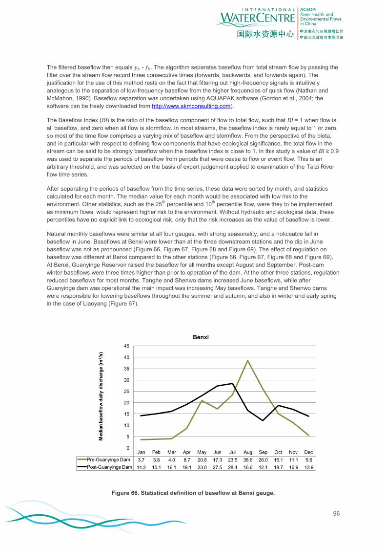
96

The filtered baseflow then equals - . The algorithm separates baseflow from total stream flow by passing the

filter over the stream flow record three consecutive times (forwards, backwards, and forwards again). The

justification for the use of this method rests on the fact that filtering out high-frequency signals is intuitively

analogous to the separation of low-frequency baseflow from the higher frequencies of quick flow (Nathan and

McMahon, 1990). Baseflow separation was undertaken using AQUAPAK software (Gordon et al., 2004; the

software can be freely downloaded from http://www.skmconsulting.com).

The Baseflow Index (BI) is the ratio of the baseflow component of flow to total flow, such that BI = 1 when flow is

all baseflow, and zero when all flow is stormflow. In most streams, the baseflow index is rarely equal to 1 or zero,

so most of the time flow comprises a varying mix of baseflow and stormflow. From the perspective of the biota,

and in particular with respect to defining flow components that have ecological significance, the total flow in the

stream can be said to be strongly baseflow when the baseflow index is close to 1. In this study a value of BI ≥ 0.9

was used to separate the periods of baseflow from periods that were cease to flow or event flow. This is an

arbitrary threshold, and was selected on the basis of expert judgement applied to examination of the Taizi River

flow time series.

After separating the periods of baseflow from the time series, these data were sorted by month, and statistics

calculated for each month. The median value for each month would be associated with low risk to the

environment. Other statistics, such as the 25th percentile and 10

th percentile flow, were they to be implemented

as minimum flows, would represent higher risk to the environment. Without hydraulic and ecological data, these

percentiles have no explicit link to ecological risk, only that the risk increases as the value of baseflow is lower.

Natural monthly baseflows were similar at all four gauges, with strong seasonality, and a noticeable fall in

baseflow in June. Baseflows at Benxi were lower than at the three downstream stations and the dip in June

baseflow was not as pronounced (Figure 66, Figure 67, Figure 68 and Figure 69). The effect of regulation on

baseflow was different at Benxi compared to the other stations (Figure 66, Figure 67, Figure 68 and Figure 69).

At Benxi, Guanyinge Reservoir raised the baseflow for all months except August and September. Post-dam

winter baseflows were three times higher than prior to operation of the dam. At the other three stations, regulation

reduced baseflows for most months. Tanghe and Shenwo dams increased June baseflows, while after

Guanyinge dam was operational the main impact was increasing May baseflows. Tanghe and Shenwo dams

were responsible for lowering baseflows throughout the summer and autumn, and also in winter and early spring

in the case of Liaoyang (Figure 67).

Figure 66. Statistical definition of baseflow at Benxi gauge.


Pre-Guanyinge Dam 3.7 3.8 4.0 8.7 20.8 17.3 23.5 38.6 26.0 15.1 11.1 5.6

Post-Guanyinge Dam 14.2 15.1 16.1 19.1 23.0 27.5 28.4 16.6 12.1 18.7 16.9 13.9

0

5

10

15

20

25

30

35

40

45

Med

ian

basefl

ow

daily d

isch

arg

e (

m3/s

)

Benxi

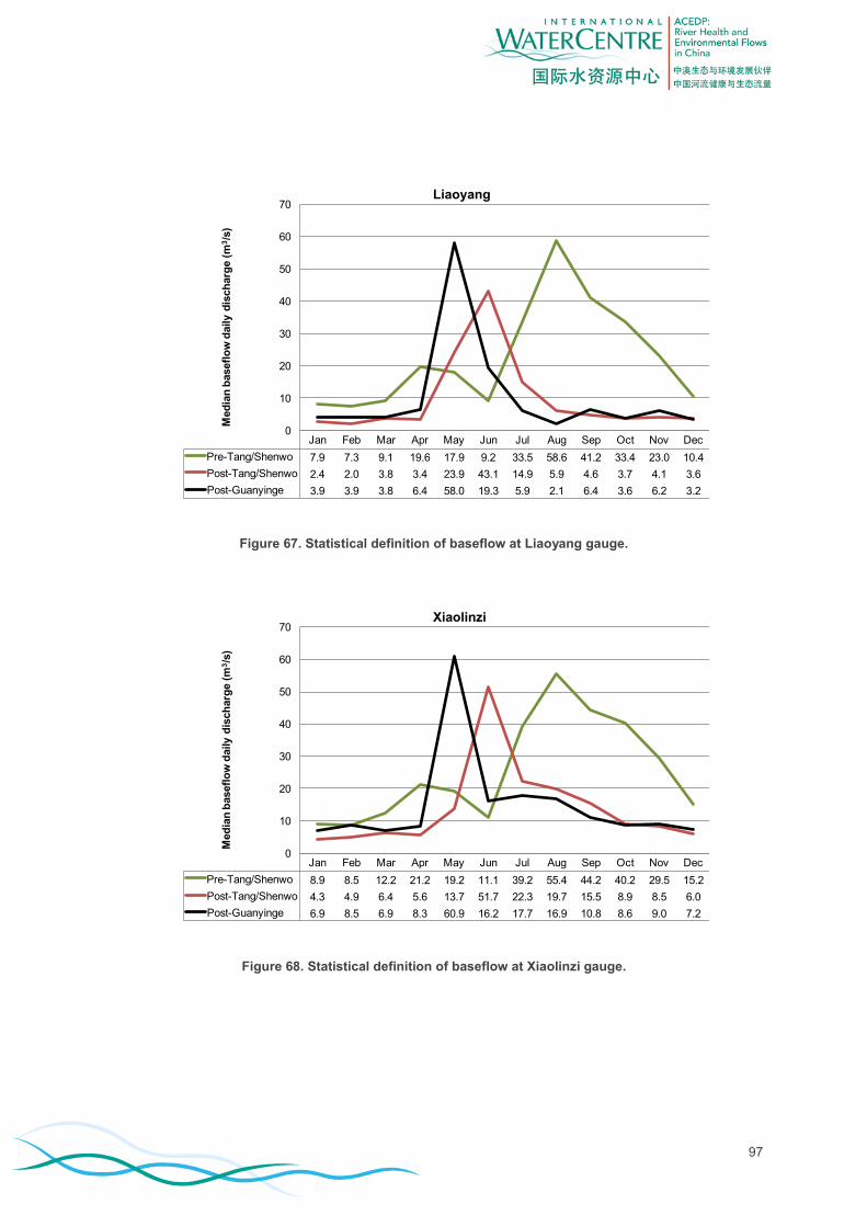
http://www.skmconsulting.com/Markets/Australia/Water--Environment/Natural-Resource-Management/AQUAPAK-Download.aspx

97

Figure 67. Statistical definition of baseflow at Liaoyang gauge.

Figure 68. Statistical definition of baseflow at Xiaolinzi gauge.


Pre-Tang/Shenwo 7.9 7.3 9.1 19.6 17.9 9.2 33.5 58.6 41.2 33.4 23.0 10.4

Post-Tang/Shenwo 2.4 2.0 3.8 3.4 23.9 43.1 14.9 5.9 4.6 3.7 4.1 3.6

Post-Guanyinge 3.9 3.9 3.8 6.4 58.0 19.3 5.9 2.1 6.4 3.6 6.2 3.2

0

10

20

30

40

50

60

70

Med

ian

basefl

ow

daily d

isch

arg

e (

m3/s

)

Liaoyang


Pre-Tang/Shenwo 8.9 8.5 12.2 21.2 19.2 11.1 39.2 55.4 44.2 40.2 29.5 15.2

Post-Tang/Shenwo 4.3 4.9 6.4 5.6 13.7 51.7 22.3 19.7 15.5 8.9 8.5 6.0

Post-Guanyinge 6.9 8.5 6.9 8.3 60.9 16.2 17.7 16.9 10.8 8.6 9.0 7.2

0

10

20

30

40

50

60

70

Med

ian

basefl

ow

daily d

isch

arg

e (

m3/s

)

Xiaolinzi

98

Figure 69. Statistical definition of baseflow at Tangmazhai gauge.

Cease to flow events Here the term “cease to flow” is used to describe the hydrological condition when the river stops flowing at a river

gauge, but water may remain in pools.

Cease to flow only occurred in the hydrological records of Liaoyang station, in Reach 2 (Figure 70). Here, cease

to flow was rare prior to regulation by dams. After operation of Tanghe and Shenwo Reservoirs began, cease to

flow occurred more often, and for March, June, July, August and September at least one quarter of years had at

least one cease to flow event (Figure 70). The total duration of cease to flow was highest in March, at just over 10

percent of the time. After operation of Guanyinge Reservoir began, cease to flow did not occur from December to

March (and also May), but the duration and frequency of cease to flow increased in the other months (Figure 70).

From the ecological health perspective, perhaps the critical aspect of cease to flow duration is the total duration

of cease to flow and the duration of the longest cease to flow spell each year. In the Taizi River at Liaoyang, in

years when the river ceased to flow, the majority of the dry days were accounted for in one continuous spell

(Figure 71).

Flow events (pulses and floods) Flows above baseflow can be described using traditional flood frequency analysis, which predicts the return

interval of events of a given magnitude (Gordon et al., 2004, pp. 204-211). In environmental flows assessment, it

is usually important to know about the duration and timing of these events, as well as their frequency. The most

appropriate analysis for this purpose is spells analysis, which involves selecting a threshold discharge and

analysing the frequency, timing and duration characteristics of all the flows above (or below) the threshold

(Gordon et al., 2004, pp. 218-219). Spells analysis can be performed by AQUAPAK software (Gordon et al., 2004;

the software can be freely downloaded from http://www.skmconsulting.com).


Pre-Tang/Shenwo 9.3 8.6 10.8 19.4 20.0 18.6 17.1 65.3 45.3 33.2 31.0 16.1

Post-Tang/Shenwo 10.3 10.0 13.1 11.3 16.1 59.3 35.1 32.7 25.6 18.0 17.1 11.6

Post-Guanyinge 12.6 13.3 12.8 13.6 42.8 18.8 25.8 26.6 23.5 17.7 16.4 13.6

0

10

20

30

40

50

60

70

Med

ian

basefl

ow

daily d

isch

arg

e (

m3/s

)

Tangmazhai

http://www.skmconsulting.com/Markets/Australia/Water--Environment/Natural-Resource-Management/AQUAPAK-Download.aspx

99

Figure 70. Frequency of cease to flow conditions at Liaoyang for the three regulation periods when cease to flow occurred.

Figure 71. Time series of annual peak duration cease to flow spell, and total days of cease to flow for each year for Liaoyang station. Note that the y-axis is scaled over 365 days, so that the relative lengths of

the bars indicate the proportion of the year that the river ceased to flow.

In undertaking spells analysis it is necessary to consider event independence. For example, two spells might

occur close together in time, separated by only a minor dip below the discharge threshold. From an ecological,

chemical and geomorphological perspective this may not result in any significant disruption to the processes

associated with flows above that threshold. In this case, the two spells would not be considered independent, but

rather as a single continuous spell. Growns and Marsh (2000) used independence criteria for streams in eastern

Australia that ranged from 4 days for a small catchment (25 km2), to 10 days for a mid-sized catchment (894 km

2),

to 20 days for a large basin (60,600 km2). NRM South (2009) recommended 30 days as the independence

criterion for bankfull events in rivers in Tasmania, Australia. It is thus not possible to recommend a simple and

clear-cut criterion for independence. Beard (1974) recommended that, for large catchments (> 1,000 km2),

independence was defined by 5 days plus the natural logarithm of the square miles of catchment area, with the

additional requirement that in the interval between independent events, the flow should fall to less than 75

percent of the lower of the flood peaks. For small catchments, Potter and Pilgrim (1971) used a criterion of three

calendar days between separate flood events. These recommendations, and others noted by Kuczera and

Franks (2006), were based on hydrological factors, rather than an understanding of the ecological implications of

the length of the independence criterion. Kuczera and Franks (2006, p. 26) concluded that:

“The circumstances and objectives of each study, and the characteristics of the catchment and flood

data, should be considered in each case before a criterion is adopted. It is inevitable that the adopted

0%

10%

20%

30%

40%

50%

60%

70%

80%

90%

100%


Perc

en

t o

f ti

me c

ease t

o f

low

1/01/1953 - 30/11/1968 [Pre-Tang/Shenwo]

1/11/1972 - 30/11/1994 [Post-Tang/Shenwo]

1/12/1995 - 30/11/2007 [Post-Guanyinge]

0%

10%

20%

30%

40%

50%

60%

70%

80%

90%

100%


Perc

en

t o

f years

cease t

o f

low

1/01/1953 - 30/11/1968 [Pre-Tang/Shenwo]

1/11/1972 - 30/11/1994 [Post-Tang/Shenwo]

1/12/1995 - 30/11/2007 [Post-Guanyinge]

0

50

100

150

200

250

300

350

Days o

f cease t

o f

low

LiaoyangCumulative annual days of cease to f low

Annual peak cease to f low spell duration

100

criterion will be arbitrary to some extent… In each particular application the designer or analyst should

choose a criterion suitable to the analysis and relevant to all of the circumstances and objectives.”

For the purpose of general characterisation of the flow regime of the Taizi River, event independence was

defined in a simple way – requiring a minimum of 7 days between instances when discharge exceeded the

threshold. For the purpose of characterising environmental flow components associated with specific ecological

functions, event independence was reconsidered (see later in this report).

Spells analysis was undertaken across a range of flows. A discharge range was set for each gauging station

using a systematic method, with the lower limit corresponding to the lowest value of the flow equalled or

exceeded 75 percent of the time (25th

percentile flow) calculated for each month for the pre-dam phase, and the

upper limit corresponding to the highest value of the flow equalled or exceeded 2 percent of the time (98th

percentile flow) calculated for each month for each station for the pre-dam phase. While these are arbitrary

statistics, they adequately define the range of flow events likely to be of interest for environmental flows

assessment. The discharge range was then split into 24 classes (an arbitrary number of classes) with class width

equal in the log-transformed range (producing closer spacing, and thus more detail, in the lower flows of the

untransformed data range). Spells were not necessarily reported across all of these 24 flow classes for each

season.

The spells were characterised for each 3-month season (Table 20) and each regulation phase (Table 21). For

each station, for each season, spells were only considered if they exceeded a seasonal baseflow threshold. The

threshold was set as the lowest seasonal value of the median value of baseflow for the pre-dam phase, as

determined by baseflow separation and BI ≥ 0.9 (as previously described). This threshold was included so that

only spells exceeding natural baseflow for each season were considered, as by definition, flow events (pulses

and floods) have to exceed baseflow discharge. Finally, if there was only one spell in a period of record, it was

not included in the characterisation of spells. The spell duration was described by the median, and the spell

frequency was described as the mean number of spells per year.

Benxi At Benxi, after Guanyinge Reservoir began operation, in summer the event frequency declined for a given

discharge magnitude (Figure 72). In winter, for events exceeding 10 m3/s the frequency increased. Frequency

was not much affected in the snowmelt season. In the recession season, events were not common before

Guanyinge began operation, and afterwards, events were only of a low magnitude (Figure 72). Duration of

summer events was markedly reduced by regulation, while in the spring snowmelt season the duration increased

after regulation (Figure 73).

Liaoyang At Liaoyang, regulation had the effect of progressively shifting the event frequency and duration further from the

pre-dam condition (Figure 74 and Figure 75). The major impacts were in the summer high flow season where the

frequency of the higher events markedly reduced, and the duration of the smaller events markedly reduced.

Higher events, > 20 m3/s, were more common in winter, but events > 100 m

3/s were eliminated in autumn (Figure

74). In the spring season, event frequency was not much affected, but the duration increased (Figure 74 and

Figure 75).

Xiaolinzi At Xiaolinzi, the pattern of regulation impacts on seasonal event hydrology (Figure 76 and Figure 77) was similar

to that at Liaoyang. One of the major changes at Xiaolinzi was a reduction in the frequency of summer events

< 150 m3/s, but an increase in frequency of summer events > 150 m

3/s (Figure 76). This increase in frequency

was associated with a marked decrease in duration of events (Figure 77).

Tangmazhai The pattern of regulation impacts on hydrology was different at Tangmazhai compared to the three upstream

stations (Figure 78 and Figure 79). Prior to regulation, winter flows at Tangmazhai were not characterised by

events – it was a period of baseflow only. After regulation, the winter season was characterised by regular small

events of low duration (Figure 78 and Figure 79). In spring, for events < 300 m3/s, the frequency and duration

markedly increased after regulation (Figure 78 and Figure 79). In summer, events < 250 m3/s increased in

101

frequency after regulation, but their duration decreased (Figure 78 and Figure 79). The flow recession season

was marked by an increase in the frequency of events (Figure 79).

Figure 72. Seasonal frequency of event spells for four phases of regulation at Benxi.

0.0

0.1

0.2

0.3

0.4

0.5

0.6

0.7

0.8

0.9

1.0

1 10 100

Mean

even

t fr

eq

uen

cy (

no

./year)

Spell event threshold (m3/s)

Winter [cold and low] [Dec - Feb]

1/01/1953 - 30/11/1994 [Pre-Guanyinge Dam]

1/12/1995 - 30/11/2007 [Post-Guanyinge Dam]

0.0

0.2

0.4

0.6

0.8

1.0

1.2

1.4

1.6

10 100 1,000

Mean

even

t fr

eq

uen

cy (

no

./year)


Spring [snowmelt] [Mar - May]



0.0

0.5

1.0

1.5

2.0

2.5

10 100 1,000

Mean

even

t fr

eq

uen

cy (

no

./year)


Summer [warm and rising] [Jun - Aug]



0.0

0.2

0.4

0.6

0.8

1.0

1.2

1.4

1.6

10 100 1,000

Mean

even

t fr

eq

uen

cy (

no

./year)


Autumn [flow recession] [Sep - Nov]



102

Figure 73. Seasonal duration of event spells for four phases of regulation at Benxi.

0

5

10

15

20

25

30

35

1 10 100

Med

ian

even

t d

ura

tio

n (

days)





0

100

200

300

400

500

600

10 100 1,000M

ed

ian

even

t d

ura

tio

n (

days)





0

10

20

30

40

50

60

70

80

90

10 100 1,000

Med

ian

even

t d

ura

tio

n (

days)





0

50

100

150

200

250

300

10 100 1,000

Med

ian

even

t d

ura

tio

n (

days)





103

Figure 74. Seasonal frequency of event spells for four phases of regulation at Liaoyang.

0.0

0.2

0.4

0.6

0.8

1.0

1.2

1 10 100

Mean

even

t fr

eq

uen

cy (

no

./year)



1/01/1953 - 30/11/1968 [Pre-Tang/Shenwo]

1/11/1972 - 30/11/1994 [Post-Tang/Shenwo]

1/12/1995 - 30/11/2007 [Post-Guanyinge]

0.0

0.5

1.0

1.5

2.0

2.5

10 100 1,000

Mean

even

t fr

eq

uen

cy (

no

./year)



1/01/1953 - 30/11/1968 [Pre-Tang/Shenwo]

1/11/1972 - 30/11/1994 [Post-Tang/Shenwo]

1/12/1995 - 30/11/2007 [Post-Guanyinge]

0.0

0.5

1.0

1.5

2.0

2.5

10 100 1,000

Mean

even

t fr

eq

uen

cy (

no

./year)



1/01/1953 - 30/11/1968 [Pre-Tang/Shenwo]

1/11/1972 - 30/11/1994 [Post-Tang/Shenwo]

1/12/1995 - 30/11/2007 [Post-Guanyinge]

0.0

0.2

0.4

0.6

0.8

1.0

1.2

1.4

1.6

10 100 1,000

Mean

even

t fr

eq

uen

cy (

no

./year)



1/01/1953 - 30/11/1968 [Pre-Tang/Shenwo]

1/11/1972 - 30/11/1994 [Post-Tang/Shenwo]

1/12/1995 - 30/11/2007 [Post-Guanyinge]

104

Figure 75. Seasonal duration of event spells for four phases of regulation at Liaoyang.

0

50

100

150

200

250

300

350

1 10 100

Med

ian

even

t d

ura

tio

n (

days)



1/01/1953 - 30/11/1968 [Pre-Tang/Shenwo]

1/11/1972 - 30/11/1994 [Post-Tang/Shenwo]

1/12/1995 - 30/11/2007 [Post-Guanyinge]

0

10

20

30

40

50

60

70

10 100 1,000M

ed

ian

even

t d

ura

tio

n (

days)



1/01/1953 - 30/11/1968 [Pre-Tang/Shenwo]

1/11/1972 - 30/11/1994 [Post-Tang/Shenwo]

1/12/1995 - 30/11/2007 [Post-Guanyinge]

0

20

40

60

80

100

120

140

10 100 1,000

Med

ian

even

t d

ura

tio

n (

days)



1/01/1953 - 30/11/1968 [Pre-Tang/Shenwo]

1/11/1972 - 30/11/1994 [Post-Tang/Shenwo]

1/12/1995 - 30/11/2007 [Post-Guanyinge]

0

2

4

6

8

10

12

14

10 100 1,000

Med

ian

even

t d

ura

tio

n (

days)



1/01/1953 - 30/11/1968 [Pre-Tang/Shenwo]

1/11/1972 - 30/11/1994 [Post-Tang/Shenwo]

1/12/1995 - 30/11/2007 [Post-Guanyinge]

105

Figure 76. Seasonal frequency of event spells for four phases of regulation at Xiaolinzi.

0.0

0.2

0.4

0.6

0.8

1.0

1.2

1 10 100

Mean

even

t fr

eq

uen

cy (

no

./year)



1/01/1953 - 30/11/1968 [Pre-Tang/Shenwo]

1/11/1972 - 30/11/1994 [Post-Tang/Shenwo]

1/12/1995 - 30/11/2007 [Post-Guanyinge]

0.0

0.5

1.0

1.5

2.0

2.5

10 100 1,000

Mean

even

t fr

eq

uen

cy (

no

./year)



1/01/1953 - 30/11/1968 [Pre-Tang/Shenwo]

1/11/1972 - 30/11/1994 [Post-Tang/Shenwo]

1/12/1995 - 30/11/2007 [Post-Guanyinge]

0.0

0.5

1.0

1.5

2.0

2.5

3.0

10 100 1,000

Mean

even

t fr

eq

uen

cy (

no

./year)



1/01/1953 - 30/11/1968 [Pre-Tang/Shenwo]

1/11/1972 - 30/11/1994 [Post-Tang/Shenwo]

1/12/1995 - 30/11/2007 [Post-Guanyinge]

0.0

0.2

0.4

0.6

0.8

1.0

1.2

1.4

10 100 1,000

Mean

even

t fr

eq

uen

cy (

no

./year)



1/01/1953 - 30/11/1968 [Pre-Tang/Shenwo]

1/11/1972 - 30/11/1994 [Post-Tang/Shenwo]

1/12/1995 - 30/11/2007 [Post-Guanyinge]

106

Figure 77. Seasonal duration of event spells for four phases of regulation at Xiaolinzi.

0

50

100

150

200

250

300

350

1 10 100

Med

ian

even

t d

ura

tio

n (

days)



1/01/1953 - 30/11/1968 [Pre-Tang/Shenwo]

1/11/1972 - 30/11/1994 [Post-Tang/Shenwo]

1/12/1995 - 30/11/2007 [Post-Guanyinge]

0

10

20

30

40

50

60

70

10 100 1,000M

ed

ian

even

t d

ura

tio

n (

days)



1/01/1953 - 30/11/1968 [Pre-Tang/Shenwo]

1/11/1972 - 30/11/1994 [Post-Tang/Shenwo]

1/12/1995 - 30/11/2007 [Post-Guanyinge]

0

20

40

60

80

100

120

140

160

10 100 1,000

Med

ian

even

t d

ura

tio

n (

days)



1/01/1953 - 30/11/1968 [Pre-Tang/Shenwo]

1/11/1972 - 30/11/1994 [Post-Tang/Shenwo]

1/12/1995 - 30/11/2007 [Post-Guanyinge]

0

2

4

6

8

10

12

14

16

10 100 1,000

Med

ian

even

t d

ura

tio

n (

days)



1/01/1953 - 30/11/1968 [Pre-Tang/Shenwo]

1/11/1972 - 30/11/1994 [Post-Tang/Shenwo]

1/12/1995 - 30/11/2007 [Post-Guanyinge]

107

Figure 78. Seasonal frequency of event spells for four phases of regulation at Tangmazhai.

0.0

0.1

0.2

0.3

0.4

0.5

0.6

0.7

0.8

0.9

1.0

1 10 100

Mean

even

t fr

eq

uen

cy (

no

./year)



1/01/1953 - 30/11/1968 [Pre-Tang/Shenwo]

1/11/1972 - 30/11/1994 [Post-Tang/Shenwo]

1/12/1995 - 30/11/2007 [Post-Guanyinge]

0.0

0.5

1.0

1.5

2.0

2.5

10 100 1,000

Mean

even

t fr

eq

uen

cy (

no

./year)



1/01/1953 - 30/11/1968 [Pre-Tang/Shenwo]

1/11/1972 - 30/11/1994 [Post-Tang/Shenwo]

1/12/1995 - 30/11/2007 [Post-Guanyinge]

0.0

0.5

1.0

1.5

2.0

2.5

3.0

10 100 1,000

Mean

even

t fr

eq

uen

cy (

no

./year)



1/01/1953 - 30/11/1968 [Pre-Tang/Shenwo]

1/11/1972 - 30/11/1994 [Post-Tang/Shenwo]

1/12/1995 - 30/11/2007 [Post-Guanyinge]

0.0

0.2

0.4

0.6

0.8

1.0

1.2

1.4

10 100 1,000

Mean

even

t fr

eq

uen

cy (

no

./year)



1/01/1953 - 30/11/1968 [Pre-Tang/Shenwo]

1/11/1972 - 30/11/1994 [Post-Tang/Shenwo]

1/12/1995 - 30/11/2007 [Post-Guanyinge]

108

Figure 79. Seasonal duration of event spells for four phases of regulation at Tangmazhai.

0

50

100

150

200

250

300

350

400

1 10 100

Med

ian

even

t d

ura

tio

n (

days)



1/01/1953 - 30/11/1968 [Pre-Tang/Shenwo]

1/11/1972 - 30/11/1994 [Post-Tang/Shenwo]

1/12/1995 - 30/11/2007 [Post-Guanyinge]

0

50

100

150

200

250

300

350

10 100 1,000M

ed

ian

even

t d

ura

tio

n (

days)



1/01/1953 - 30/11/1968 [Pre-Tang/Shenwo]

1/11/1972 - 30/11/1994 [Post-Tang/Shenwo]

1/12/1995 - 30/11/2007 [Post-Guanyinge]

0

20

40

60

80

100

120

140

160

180

10 100 1,000

Med

ian

even

t d

ura

tio

n (

days)



1/01/1953 - 30/11/1968 [Pre-Tang/Shenwo]

1/11/1972 - 30/11/1994 [Post-Tang/Shenwo]

1/12/1995 - 30/11/2007 [Post-Guanyinge]

0

2

4

6

8

10

12

14

16

10 100 1,000

Med

ian

even

t d

ura

tio

n (

days)



1/01/1953 - 30/11/1968 [Pre-Tang/Shenwo]

1/11/1972 - 30/11/1994 [Post-Tang/Shenwo]

1/12/1995 - 30/11/2007 [Post-Guanyinge]

109

Rates of rise and fall The rates of rise and fall in flow are of interest in environmental flow assessment because some ecological

processes are sensitive to these characteristics of the flow regime. For example, a rising river may act as a cue

for spawning or migration behaviour (e.g. Baran, 2006), and an unnatural rate of rise might not elicit the same

response as when the rate of rise lies within the natural range. Some animals seek refuge when flows increase,

and an unnaturally rapid rate of rise might not allow sufficient time for them to avoid being washed into fast flow.

Rate of fall is also important, as an unnaturally fast rate of fall can cause stranding of animals on the margins of

streams (e.g. Cushman, 1985; Bradman, 1987; Saltviet et al., 2001), or abandonment of nests by colonial water

birds in river-connected wetlands (e.g. Leslie, 2001; Leslie and Ward, 2002).

In regulated rivers, rate of rise and fall is at least partly controllable. From the perspective of minimising water

cost, the most efficient way to achieve environmental flow targets is through imposition of rapid rates of rise and

fall. This assumes that the rise and fall period does not have a high ecological priority in terms of meeting

environmental flow objectives, and because the longer is the rise and fall period, the higher is the cost in water of

providing that flow component. Thus, from the perspective of the sensitivity of ecological processes and efficient

use of water, it is the upper limits of rates of rise and fall that are of primary interest. In some cases the

ecologically tolerable rates of rise and fall might be known, but in the absence of this knowledge the best guide is

the observed rates of rise and fall in the unimpaired flow record. As the main interest is in setting upper limits of

rates of rise and fall, the most appropriate statistic is a value higher than the median, but less than the maximum

(which would be regarded as an extreme case, and high risk to the biota). In this study the 75th

percentile was

selected as an arbitrary index of upper rates of rise and fall.

For each station, rates of rise and fall were characterised across the same range of discharge utilised for the

spells analysis. The range was divided in to the same 24 classes used for the spells analysis. Within each class,

the 75th

percentile of rise and fall was calculated.

In the Taizi River, the rates of rise and fall are closely related to discharge. The higher the discharge the higher

are the rates of rise and fall, with the rates related to discharge by a power function (Figure 80). In general, the

rates of rise are faster than rates of recession. The controlled rates of rise and fall associated with dam releases

have mostly been similar to the natural rates (as characterised in the pre-dam phase) (Figure 80).

Figure 80. Distribution of rates of rise and fall for the high-flow season rising phase (summer) and recession phase (autumn) for the pre-Guanyinge and post-Guanyinge phases of regulation at Benxi. Note

that discharge values represent data grouped within classes.

y = 0.0756x1.3079

R² = 0.9877

0

100

200

300

400

500

600

0 200 400 600 800 1,000 1,200

P75 r

ate

of

rise (

m3/s

per

day)

Mean daily discharge (m3/s)

Summer [warm and rising] [Jun - Aug] Rise



y = 0.0454x1.2787

R² = 0.9856

0

100

200

300

400

500

600

0 200 400 600 800 1,000 1,200

P75 r

ate

of

fall (

m3/s

per

day)

Mean daily discharge (m3/s)

Summer [warm and rising] [Jun - Aug] Fall



110

The natural rates of 75th percentile rise and fall (based on pre-dam historical data) were described as power

functions of discharge, with each relationship significant at α ≤ 0.05 (Table 28). These equations could be used to

set the maximum rates of rise and fall for controlled dam releases. Note that as the discharge is increased and

decreased over an event cycle, the appropriate rate of rise and fall changes each day. Also, these equations can

be used as objective functions to test compliance of a flow regime with respect to rates of rise and fall.

Table 28. Relationships describing the 75

th percentile rates of rise and fall as a function of discharge in the pre-

dam phase for four gauging stations on the Taizi River.

Station Season Rate of rise (R) as function of discharge (Q) (m3/s per day)

Rate of fall (F) as function of discharge (Q) (m3/s per day)

Benxi Winter (Dec-Feb) R = 0.0563 Q1.3558

F = 0.0499 Q1.2531

Spring (Mar-May) R = 0.0657 Q1.3118

F = 0.0567 Q1.2205

Summer (June-Aug) R = 0.0756 Q1.3079

F = 0.0454 Q1.2787

Autumn (Sep-Nov) R = 0.0498 Q1.3330

F = 0.0470 Q1.2231

Liaoyang Winter (Dec-Feb) R = 0.0582 Q1.3035

F = 0.0468 Q1.2485


F = 0.0657 Q1.2016


F = 0.1898 Q1.0226


F = 0.0176 Q1.3759

Xiaolinzi Winter (Dec-Feb) R = 0.0286 Q1.4167

F = 0.0322 Q1.2859


F = 0.0390 Q1.2753


F = 0.1119 Q1.0939


F = 0.0146 Q1.3770

Tangmazhai Winter (Dec-Feb) R = 0.0202 Q1.4610

F = 0.0275 Q1.2902


F = 0.0426 Q1.2501


F = 0.0671 Q1.1497


F = 0.0251 Q1.2617

Eco-hydraulic information

Data from cross-section locations

For this rapid environmental flows assessment, no specific morphological surveys were undertaken for the

purpose of hydraulic modelling. Any environmental flows study on an important river with valuable ecological and

social assets, and a high degree of competition for scarce water resources, warrants inclusion of a detailed

investigation of hydraulic habitat availability. The Taizi River may well be a candidate for such an investigation,

but the focus of the present study was on developing a methodology for assessing the hydrological component of

river health, not on undertaking a comprehensive environmental flows assessment.

Basic hydraulic data are available at every hydrological gauging station. River discharge is measured indirectly

through frequent monitoring of river stage height (which is easy to measure) and every so often undertaking

detailed gaugings of discharge (which is much more time consuming and difficult), and then relating the gauged

discharges to the river stage heights through a rating curve. In combination with a surveyed cross-section, which

can usually be obtained from nearby gauging stations, it is possible to interpret the eco-hydraulic needs of certain

ecological assets. Rating data and cross-section data were obtained for the four gauging stations on the Taizi

River main stem (Figure 81). The 2001 cross-sections used here were previously published by Zhang et al.

(2007).

A long profile of the main stem of the river was drawn from the SRTM DEM (Figure 82), and this allowed an

estimate of channel slope in the vicinity of the gauges (Table 29).

111

Figure 81. Taizi River basin, showing locations of environmental flow assessment sites. Upper image is derived from SRTM and shows topography, and lower image is Landsat TM showing land use.

Particle size of the bed material was sampled as part of the river health assessment field surveys at sites in the

vicinity of the stream flow gauges (Figure 83). At each site, sediment was sampled and sieved at three locations.

Here, the data from the three locations were combined to produce one size distribution per site. The sample data

from site T39 (Liaoyang) were not used, as a total of only 45 g of sediment was collected. The data from site T40

appeared to contain either an erroneous data point, or one large stone >256 mm and weighing 5 kg was sampled.

It is possible that such large stones exist in the river, but this individual was regarded as an outlier (and

eliminated), as it was the only stone of this size sampled between Benxi and Liaoyang. There was a distinctive

fining of bed material from downstream of Shenwo dam (T33) to upstream of Beisha River junction (T40) (Figure

84, Figure 61). Data from sample site T20 was selected to represent Benxi cross-section and sample site T40

was selected to represent Liaoyang cross-section (Table 30). Upstream of Beisha River junction (towards

Liaoyang) the river bed was composed of gravels and cobbles, and downstream of the junction (towards Xiaolinzi)

the bed was composed entirely of material smaller than 4 mm (Figure 84). It appears that the Beisha River

supplied sand-sized material to the river, but also, the slope of the Taizi River reduces noticeably in this vicinity

112

(Figure 82), so here the river loses competency to transport gravels and cobbles. The sediment fraction less than

4 mm diameter was not sized, so sediment size statistics were estimated for Xiaolinzi and Tangmazhai sites

(Table 30). Frings (2008) reported that downstream fining was normal in sand-bed rivers. The Rhine, Mississippi

and Ganges rivers have downstream fining rates in the median particle diameter ( ) of 0.8% per km, 0.08% per

km and 0.02% per km, respectively. So, if the median particle diameter at Xiaolinzi is assumed to be 1 mm, then

at Tangmazhai (30 km downstream) these data suggest that might have fined to between 0.99 and 0.75 mm.

Based on visual field observations, the higher value of fining (25% reduction) was used here. The particle size

statistics adopted for Xiaolinzi and Tangmazhai, and to a lesser extent Benxi and Liaoyang, are preliminary

estimates that need to be updated using measured data from field collected samples.

Figure 82. Taizi River long profile, derived from SRTM.

Figure 83. Taizi River field sampling locations.

Tangmazhaigauge

Xiaolinzigauge

Liaoyanggauge

ShenwoDam

Benxigauge

GuanyingeDam

Guanmenlazi Reservoir

-100

0

100

200

300

400

500

600

700

0 50 100 150 200 250 300 350 400

Ele

vati

on

(m

ab

ove s

ea level)

Distance upstream from Hun River junction (km)

113

Table 29. Estimate of channel slope for the Taizi River gauges based on long profile derived from SRTM.

Gauge Slope estimate

Benxi 0.0013700

Liaoyang 0.0005740

Xiaolinzi 0.0001242

Tangmazhai 0.0000884

Figure 84. Particle size distribution of bed material at sampled sites in the vicinity of Benxi and Liaoyang. At sites downstream of Beisha River junction the bed was composed entirely of sand.

Table 30. Particle size statistics for bed material from sampled sites selected to represent the cross-sections. The values for Xiaolinzi and Tangmazhai are estimated, as particles less than 4 mm were not

sized, but local knowledge suggested that the bed material was mostly coarse sand, and fining downstream.

Parameter Benxi (T20) Liaoyang (T40) Xiaolinzi Tangmazhai

(mm) 35 8 1.0 0.75

(mm) 119 76 2.0 1.5

(mm) 256 128 4.0 3.0

The cross-section data have variable coverage of the width of the river corridor (Figure 85, Figure 86, Figure 87

and Figure 88). It is apparent that Benxi (Figure 85) and Liaoyang (Figure 86) locations are in weir ponds.

Xiaolinzi (Figure 87) and Tangmazhai (Figure 88) are free flowing sections. Benxi and Liaoyang are in urban

areas, while Xiaolinzi and Tangmazhai are in rural areas. The Xiaolinzi and Tangmazhai cross-sections and

aerial photographs indicate farmland within high dikes about 0.9 – 1.0 km apart, and smaller dikes built up around

the channel bank. Benxi and Liaoyang appear to have very little connected floodplain, with dikes close to the

edge of the channel, and beyond that lies densely settled urban land.

0%

10%

20%

30%

40%

50%

60%

70%

80%

90%

100%

1 10 100 1000

Perc

en

tag

e o

f sam

ple

fin

er

than

siz

e

Particle size (mm)

T19 Benxi T20 Benxi T33 Liaoyang T40 Liaoyang

114

Figure 85. Aerial photograph and cross-section from vicinity of Benxi gauge.

115

Figure 86. Aerial photograph and cross-section from vicinity of Liaoyang gauge.

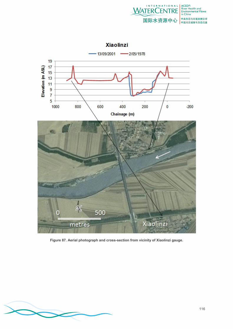
116

Figure 87. Aerial photograph and cross-section from vicinity of Xiaolinzi gauge.

117

Figure 88. Aerial photograph and cross-section from vicinity of Tangmazhai gauge.

118

Hydraulic data From the rating curve, and knowledge of the river slope, it was possible to develop hydraulic relationships for the

gauges. The highest flow considered in the analysis was a mean daily discharge of 4,000 m3/s. Over the

historical record (1951 – 2007) this flow was equalled or exceeded very infrequently in the Taizi River (1 time at

Benxi in Aug 1960, 2 times at Liaoyang in Aug 1960 and Aug 1964, and not at Xiaolinzi or Tangmazhai). Data

concerning peak instantaneous discharge was not made available to this project, but it is known that peak

discharges far exceed mean daily discharges. For example, the Taizi River suffered floods exceeding

10,000 m3/s on seven occasions since 1870 (JICA, 2000). Of these, the largest was on 5 August 1960, when the

flow reached 18,100 m3/s at Liaoyang (the maximum mean daily flow of this flood was only 5,820 m

3/s at

Liaoyang). JICA (2000) reported that this event was described as having a recurrence interval of 150 years.

Notable flood peaks also occurred 1975 and 1985 (JICA, 2000).

Cross-sections were available for 1978 and 2001 for the four gauge sites. While the cross-sections showed a

degree of morphological change between these years (Figure 85, Figure 86, Figure 87 and Figure 88), they were

similar enough that there was minimal difference in the hydraulics. The 2001 data were used here, except for the

case of Xiaolinzi, where the 2001 channel survey data were extended to the floodplain using the 1978 survey

data. Selected discharge and corresponding water elevation data extracted from the records of 2001, together

with some data for higher events taken from the flood of 1995, were used to develop rating relationships between

discharge and stage height for each gauge.

For each site, the relationship between discharge and stage height was taken directly from the rating data.

Velocity at any stage height was calculated as mean velocity, or discharge divided by cross-sectional area.

Wetted perimeter was calculated at any stage height as the distance along the channel bed. Shear stress at the

bed ( ) is represented by:

( 31 )

where:

γ = Unit weight of water (9,800)

R = Hydraulic radius

S = Energy slope

Hydraulic radius is cross-sectional area divided by the wetted perimeter. Energy slope was assumed to be equal

to the bed slope measured from the DEM (Table 29). Slope was assumed constant with discharge for the freely

flowing Xiolinzi and Tangmazhai sites. For the Benxi and Liaoyang sites, which were in weir pools, slope was

varied from zero at no discharge up to the DEM derived slope at 4,000 m3/s. These are generalisations made in

the absence of field data or hydraulic model results.

Benxi The channel between the tailwaters of Shenwo Reservoir and Guanyinge dam (Figure 61) is regulated by low

weirs. In this section there are 17 low weirs ranging in height from 2 to 5 m and storage capacities ranging from

0.78 to 4.5 × 106 m

3 (Figure 89, CRAES, 2010). Aerial photographs (http://maps.google.com.au) indicate that at

low flow the weir pools range from about 200 m to about 2,000 m long. At low flows, about half of the reach is

free-flowing and the other half is in weir pools. Assuming full mixing, the water in the pools would be fully

exchanged over a 24 hour period at flow rates between 9 and 52 m3/s, depending on weir pool capacity.

http://maps.google.com.au/

119

Figure 89. Weirs, dams and reservoirs in the Taizi Basin. Source: CRAES (2010).

The cross-section available for Benxi was apparently surveyed in a weir pool, because the gauge rating data

(discharge versus water elevation) indicated that discharge approached zero at an elevation of about 0.9 m

higher than the thalweg. At this site, the hydraulics were modelled under two sets of conditions. The first

assumed weir pool conditions, and the second assumed free flowing conditions. Under the weir pool assumption,

the rating data from the gauge determined the discharge and velocity. The shear stress was calculated as a

function of the hydraulic radius and the energy slope. Energy slope was assumed to follow water surface slope,

which was assumed to increase incrementally with stage height from zero at zero stage to 0.00137 (general

channel slope from the DEM) at the stage corresponding to 4,000 m3/s.

Under the assumption of no weir, discharge was estimated using the Manning equation. Assuming that at

4,000 m3/s the weir would be fully drowned and hydraulically irrelevant, a Manning’s n value of 0.0255 gave

identical stage and discharge for the with- and without-weir conditions. At low flows the appropriate Manning’s n

for this gravel/cobble bed stream was estimated to be 0.05. Manning’s n was assumed to increase incrementally

with stage height from 0.05 at zero stage to 0.0255 at the stage corresponding to 4,000 m3/s. Energy slope was

assumed constant with stage height at 0.00137 (general channel slope from the DEM).

At Benxi, under pre-dam hydrology, there was a large difference in the wetted perimeter under baseflow

conditions in the high flow period compared to the low flow period (Figure 90). The frequently occurring flow

events would be well contained within the artificial levees.

120

Figure 90. Hydraulic relationships for Benxi cross-section, showing levels corresponding to a selection of baseflows and flow events for the warm rising flow period (June - August). The cross-section is in a

weir pool; the dashed lines are modelled relationships assuming no weir present.

Liaoyang The channel between Shenwo dam and Beisha River junction (Figure 61) is regulated by some low weirs. In this

section there are 9 low weirs (Figure 89, CRAES, 2010). Aerial photographs (http://maps.google.com.au) indicate

that at low flow the weir pools range from about 200 m to about 3,000 m long. At low flows, more than half of the

reach is free-flowing and the rest is in weir pools.

The cross-section available for Liaoyang was apparently surveyed in a weir pool, because the gauge rating data

(discharge versus water elevation) indicated that discharge approached zero at an elevation of about 2.2 m

higher than the thalweg. At this site, the hydraulics were modelled under two sets of conditions. The first

assumed weir pool conditions, and the second assumed free flowing conditions. Under the weir pool assumption,

the rating data from the gauge determined the discharge and velocity. The shear stress was calculated as a

function of the hydraulic radius and the energy slope. Energy slope was assumed to follow water surface slope,

which was assumed to increase incrementally with stage height from zero at zero stage to 0.000574 (general

channel slope from the DEM) at the stage corresponding to 4,000 m3/s.

0

2

4

6

8

10

0 50 100 150 200 250 300

Sta

ge (

m)

Chainage (m)

Benxi High flow 1:2 year (pre-dam) High flow 1:1 year (pre-dam) High flow 2:1 yr (pre-dam)

Aug baseflow (pre-dam) no weir Feb baseflow (pre-dam) no-weir

0.0

0.5

1.0

1.5

2.0

2.5

3.0

3.5

4.0

4.5

0 1 2 3 4 5 6 7

Mean

velo

cit

y (

m/s

)

Stage (m)

Velocity

Assuming no weir

0

10

20

30

40

50

60

70

0 1 2 3 4 5 6 7

Bed

sh

ear

str

ess (

N/m

2)

Stage (m)

Shear stress

Assuming no weir

0

50

100

150

200

250

300

0 1 2 3 4 5 6 7

Wett

ed

peri

mete

r (m

)

Stage (m)

Wetted perimeter

0

500

1,000

1,500

2,000

2,500

3,000

3,500

4,000

4,500

0 1 2 3 4 5 6 7

Dis

ch

arg

e (

m3/s

)

Stage (m)

Discharge

Assuming no weir

http://maps.google.com.au/

121

Under the assumption of no weir, discharge was estimated using the Manning equation. Assuming that at

4,000 m3/s the weir would be fully drowned and hydraulically irrelevant, a Manning’s n value of 0.028 gave

identical stage and discharge for the with- and without-weir conditions. At low flows the appropriate Manning’s n

for this gravel/cobble bed stream was estimated to be 0.05. Mannings n was assumed to increase incrementally

with stage height from 0.05 at zero stage to 0.028 at the stage corresponding to 4,000 m3/s. Energy slope was

assumed constant with stage height at 0.000574 (general channel slope from the DEM).

At Liaoyang, under pre-dam hydrology, the low bench on the right side of the channel (Figure 91) was inundated

under high flow period baseflows in some areas (Figure 91). The frequently occurring flow events would be

contained within the artificial levees, but there would be a chance of floodplain inundation because the

instantaneous flood peak is significantly higher than the mean daily discharge.

Figure 91. Hydraulic relationships for Liaoyang cross-section, showing levels corresponding to a selection of baseflows and flow events for the warm rising flow period (June - August). The cross-section

is in a weir pool; the dashed lines are modelled relationships assuming no weir present.

0

2

4

6

8

10

0 100 200 300 400 500 600 700 800

Sta

ge (

m)

Chainage (m)

Liaoyang High flow 1:2 year (pre-dam) High flow 1:1 year (pre-dam) High flow 2:1 yr (pre-dam)

Aug baseflow (pre-dam) no weir Feb baseflow (pre-dam) no-weir

0.0

0.5

1.0

1.5

2.0

2.5

3.0

0 1 2 3 4 5 6 7 8

Mean

velo

cit

y (

m/s

)

Stage (m)

Velocity

Assuming no weir

0

5

10

15

20

25

30

0 1 2 3 4 5 6 7 8

Bed

sh

ear

str

ess (

N/m

2)

Stage (m)

Shear stress

Assuming no weir

0

50

100

150

200

250

300

350

0 1 2 3 4 5 6 7 8

Wett

ed

peri

mete

r (m

)

Stage (m)

Wetted perimeter

0

500

1,000

1,500

2,000

2,500

3,000

3,500

4,000

4,500

0 1 2 3 4 5 6 7 8

Dis

ch

arg

e (

m3/s

)

Stage (m)

Discharge

Assuming no weir

122

Xiaolinzi The Xiaolinzi reach (Beisha River junction to Sha River junction) (Figure 61) is not regulated by weirs. The

channel is lined by artificial levees, but unlike the two upstream cross-sections which were within urban areas,

here the floodplain is farmland. In winter the channel meanders within large side attached sand bars, while in the

high flow period these are often inundated. At Xiaolinzi cross-section, under pre-dam hydrology, the peak high

flow period baseflows would have inundated the large bar on the right side of the channel, but most of the time it

would have been exposed (Figure 92). The frequently occurring flow events would be contained within the

artificial levees, but the 1 in 2 year ARI event would probably inundate the floodplain due to the instantaneous

flood peak being significantly higher than the mean daily discharge.

Figure 92. Hydraulic relationships for Xiaolinzi cross-section, showing levels corresponding to a selection of baseflows and flow events for the warm rising flow period (June - August). The cross-section


Tangmazhai The Tangmazhai reach (Sha River junction to Hun River junction) is not regulated by weirs. The channel is lined

by artificial levees, but like the Xiaolinzi cross-section, the floodplain is farmland. At Tangmazhai cross-section,

0.0

0.2

0.4

0.6

0.8

1.0

1.2

1.4

1.6

1.8

2.0

0 1 2 3 4 5 6 7 8 9 10

Mean

velo

cit

y (

m/s

)

Stage (m)

Velocity

0

1

2

3

4

5

6

7

8

0 1 2 3 4 5 6 7 8 9 10

Bed

sh

ear

str

ess (

N/m

2)

Stage (m)

Shear stress

0

100

200

300

400

500

600

700

800

900

0 1 2 3 4 5 6 7 8 9 10

Wett

ed

peri

mete

r (m

)

Stage (m)

Wetted perimeter

0

500

1,000

1,500

2,000

2,500

3,000

3,500

4,000

0 1 2 3 4 5 6 7 8 9 10

Dis

ch

arg

e (

m3/s

)

Stage (m)

Discharge

0

2

4

6

8

10

0 100 200 300 400 500 600 700 800 900

Sta

ge (

m)

Chainage (m)

Xiaolinzi High flow 1:2 year (pre-dam) High flow 1:1 year (pre-dam) High flow 2:1 yr (pre-dam)

Aug baseflow (pre-dam) Feb baseflow (pre-dam)

123

under pre-dam hydrology, the peak high flow period baseflows would have inundated the bars in the channel, but

under low flow baseflow conditions, some bedforms would have been exposed (Figure 93). The frequently

occurring flow events would be contained within the artificial levees, but the 1 in 2 year ARI event would probably

have inundated the floodplain due to the instantaneous flood peak being significantly higher than the mean daily

discharge.

Figure 93. Hydraulic relationships for Tangmazhai cross-section, showing levels corresponding to a selection of baseflows and flow events for the warm rising flow period (June - August). The cross-section


It should be pointed out that although the hydraulic relationships (Figure 93) were derived from stage height and

discharge data from the gauging station, there is uncertainty in the results, as evidenced by a plot of discharge

versus mean velocity at Tangmazhai gauge by Feng et al. (2010a) (Figure 94). Their relationship shows much

higher velocities than indicated by the gauge rating data. This difference could arise if the cross-section made

available to this study was not surveyed directly at the gauge, or was not surveyed with sufficient detail (which

would make the estimates of cross-sectional area, and hence mean velocity, incorrect).

0.0

0.2

0.4

0.6

0.8

1.0

1.2

1.4

0 1 2 3 4 5 6 7 8

Mean

velo

cit

y (

m/s

)

Stage (m)

Velocity

0.0

0.5

1.0

1.5

2.0

2.5

3.0

3.5

4.0

4.5

5.0

0 1 2 3 4 5 6 7 8

Bed

sh

ear

str

ess (

N/m

2)

Stage (m)

Shear stress

0

50

100

150

200

250

300

350

0 1 2 3 4 5 6 7 8

Wett

ed

peri

mete

r (m

)

Stage (m)

Wetted perimeter

0

200

400

600

800

1,000

1,200

1,400

1,600

0 1 2 3 4 5 6 7 8

Dis

ch

arg

e (

m3/s

)

Stage (m)

Discharge

0

2

4

6

8

10

300 400 500 600 700 800 900 1000 1100

Sta

ge (

m)

Chainage (m)

Tangmazhai High flow 1:2 year (pre-dam) High flow 1:1 year (pre-dam)

Aug baseflow (pre-dam) Feb baseflow (pre-dam)

124

Figure 94. Relationship between mean velocity and discharge at Tangmazhai gauge published by Feng et al. (2010a).

Comprehensive environmental flow objectives

Introduction

Environmental flow objectives were set for maintaining physical form (geomorphological) (Table 39), vegetation

(Table 40), fish (Table 41), and macroinvertebrate (Table 42) ecosystem categories. These should be considered

preliminary and tentative in nature, as for many of the species the data concerning hydraulic habitat requirements

are sparse. For all of these flow event-dependent objectives, it is assumed that rate of rise and fall should fall

within the natural range.

Surveys specific to the information needs of an environmental flow assessment have not been undertaken in the

Taizi River. Yu (1996) divided northern China into five aquatic vegetation-based regions on the basis of indicator

plants. The classification considered the co-evolutionary relationships between plants and animals (fish and

molluscs), climate and geomorphic factors. The Liao River basin was distinctive in terms of certain diagnostic

plants, and associated fish and molluscs (Table 31). Yu (1996) subdivided the Liao River aquatic vegetation-

based region into three sub-regions.

In the sub-region containing the Taizi River, Yu (1996) described the typical fauna as Gobio rivuloides (prefers

sandy bottom in shallow slow current), Saurogobio dumerili, Odontobutis obscura and Parafossarulus striatulus

(freshwater snail). In this sub-region, aquatic plants totalled 93 species. Typical plants were Ceratophyllum spp.

endemic to the northeast, Carex spp., Eichhornia crassipes (water hyacinth), Vallisneria spp., Euryale ferox

(water lily), Sparganium stoloniferum (simplestem bur-reed), Ranunculus trichophyllum (threadleaf crowfoot) and

Trapa maximowiczii (Xi Guo Ye Ling).

Some of the species that occur in the Taizi River may be more flow-sensitive than others, and these would make

better indicator species for environmental flow assessments. An example of a species that is not particularly flow

sensitive is the snail Semisulcospira libertine; its drift and upstream movement requires only normal baseflow,

and it is not enhanced by flow pulses (Kumiko and Misako, 2004). However, this snail is known to prefer pool

over fast flowing habitat (Furujo and Tomiyama, 2000), so any environmental flow objective would have to focus

on availability of pool habitat as a function of flow. Research into the flow sensitivity of the various flora and fauna

in the river system will improve the reliability of environmental flow assessments.

Mean velocity (m/s)

Dis

char

ge

(m3/s

)

125

Table 31. Diagnostic aquatic plants and associated fish and molluscs of the Liao River region of north east China (Yu, 1996), with brief descriptions sourced from various online databases.

Plants Fish Molluscs

Ceratophyllum manshuricum (submersed, rootless, found in backwaters and ponds )

Hemibarbus longirostris (benthopelagic, freshwater)

Bellamya purificata (freshwater mud snail)

Caldesia parnassifolia (floating plant on edge of water bodies)

Abbottina liaoningensis (demersal, freshwater)

Assiminea lalericera (brackish water and saltmarsh snail)

Blyxa japonica

(submerged roots, found in stagnant, shallow pools and marshes)

Phoxinus oxycephalus

(demersal, freshwater)

Semisulcospira libertina

(freshwater snail)

Hydrocharis dubia (perennial with emergent and floating leaves; stolons rooted in shallow water)

Microphysogobio yaluensis (benthopelagic, freshwater)

Lamprotula gottschei (freshwater mussel)

Limnophila sessiliflora (mostly submersed, partly emersed, rooted in substrate in water up to 4 m deep)

Rostrogobio liaohensis (benthopelagic, freshwater)

Corbicula nitens (freshwater and brackish water clam)

Development of geomorphological flow objectives There is a general belief among river ecologists that high physical heterogeneity delivers greater diversity of

habitats, which is beneficial to the biota (e.g. Kemp et al., 1999; Jowett and Duncan, 1990; Dollar, 2000;

Chessman et al., 2006). Bartley and Rutherfurd (2005) summarised that:

“…physical diversity and heterogeneity in streams is known to correlate well with biological diversity (e.g.

Chisholm et al., 1976; Downes et al., 1998; Gorman and Karr, 1978; Ward et al., 2001) and reduced

surface roughness and heterogeneity can in turn reduce species diversity, population abundance and

recruitment (McCoy and Bell, 1991; Kolasa and Rollo, 1991). Thus, physical diversity is acknowledged

as one indicator of stream health (Norris and Thoms, 1999) and diversity of habitat.”

River health is also dependent on the dynamic nature of the physical environment (Richards et al., 2002).

Disturbance is widely recognized as a key process regulating riverine ecosystem structure and function (Resh et

al., 1988; Townsend, 1989; Poff et al., 1997; Lake, 2000). Disturbance can be caused by hydrological events, but

also by associated geomorphological events, such as bed and bank instability. For example, Florsheim et al.

(2008) found that bank erosion is an important component of the natural disturbance regime of river systems and

is integral to long-term geomorphic evolution of fluvial systems and to ecological sustainability.

A diverse physical habitat accommodates a wide range of preferences and tolerances of hydraulic conditions of

biota. Also, physical irregularity potentially provides cover, and offers refugia at times of high flows when

intolerably high velocities and shear stresses may occur in the main body of the flow. Consideration of fluvial

geomorphology is important in environmental flow assessments because the health of the biota is reliant on the

presence of a certain distribution of physical habitat in space and time. The flow-geomorphology-ecology

relationship is underpinned by three fundamental concepts:

1. A spatially diverse physical environment will give rise to a spatially diverse range of hydraulic habitats at

any time,

2. A hydrologically dynamic flow regime generates variability in the pattern of hydraulic habitat available

over time by activating the full range of physical diversity present in the entire channel and floodplain,

and

3. Channel dynamism gives rise to diversity of the physical environment.

Of these, it can be assumed that the first two are implicitly covered by flow-ecology objectives, which express the

need for a certain variability and area of physical habitat to be available at certain times to provide for the needs

of the ecological assets. Geomorphological flow objectives then centre on maintaining channel dynamism.

126

Ecologically-positive channel dynamism is associated with the processes of: creation of a range of channel forms

(e.g. benches, bars, undercuts, pools and riffles) through sediment supply, transport and deposition processes

(e.g. Yarnell et al., 2006; McBain and Trush, 1997); bank erosion (e.g. Florsheim, 2008); bed material

mobilisation (e.g. Reiser et al., 1985; Gippel, 2001, Dollar, 2000; Schmidt and Potyondy, 2004); flushing of fine

sediment from the bed surface and hyporheic zone (e.g. Rowntree and Wadeson, 1999; Hancock and Boulton,

2005); vegetation succession in association with geomorphic disturbance (e.g. Hupp and Osterkamp, 1996;

Richards et al., 2002); and large woody debris dynamics (e.g. Gippel, 1995; Montgomery et al., 2003; Lester and

Boulton, 2008).

The common geomorphological objectives for environmental flows listed by Wilcock et al. (1996) are generally

agreed by others (e.g. Hill et al., 1991; Brookes, 1995; McBain and Trush, 1997; Brizga, 1998; Gippel, 2001b). A

comprehensive list of objectives includes:

1. Removing fine sediment from pools used for rearing habitat (in streams where pools are a distinctive

characteristic).

2. Removing fine sediment from gravel and cobble substrates used for spawning, juvenile cover and

invertebrate food production (in streams with coarse-bed material).

3. Entrain coarse sediment on the bed surface, permitting the removal of subsurface fine material and

producing a loose structure (in streams with coarse-bed material).

4. Entrainment of sediment through the active channel to prevent the establishment of mature vegetation

and thus preventing a corresponding loss of aquatic habitat and channel capacity. Depending on the

relative resistance of the bed material and the strength of the plants, the same effect might be achieved

through direct flow damage to, or removal of, vegetation.

5. Erosion of the riverbank to maintain topographic diversity and provide a supply of coarse sediment and

large wood (in streams where coarse sediment and large wood are characteristic).

6. Scouring sand from pools and maintenance of pool-and-riffle morphology (in streams where pool-riffle

morphology is a distinctive characteristic).

7. Maintaining active channel width and topographic diversity.

8. Maintaining valley-scale features: channel pattern (straight, meandering, braided, anastomosing) and

overall dimensions, and floodplain features such as wetlands.

Methods for estimating the flows required to achieve the above objectives can be found in the literature (e.g.

Dollar, 2000; Gippel, 2001b; Schmidt and Potyondy, 2004). The methods fall into the categories of rules of thumb,

mimicking natural flows, and empirical and semi-empirical sediment transport equations. Rules of thumb should

be reserved for cases lacking hydraulic and sediment data; as a starting point, the frequency, duration and rate of

rise and fall of events to meet geomorphological objectives can be based on the characteristics of such events as

they occurred in the unimpaired flow regime; and provided sufficient hydraulic and sediment data are available,

the flow magnitudes required to meet some geomorphological objectives can be derived using established

equations.

Hill et al. (1991) suggested that the flow which maintains the important ecological and small-scale morphological

characteristics of a channel corresponds to the level where plants show sensitivity to inundation or where rock

surfaces are abraded by bedload. This was called the channel maintenance discharge. While bankfull flow is

defined in terms of channel geometry (i.e. the flow that fills the channel to the bank top), the dominant, or

effective, discharge is the flow that carries the majority of the sediment load over a long period of time (Gordon,

1995). The effective discharge could be said to be the cause, and the bankfull channel geometry is the effect.

Thus, it is not surprising that the peak effective discharge often coincides with the bankfull discharge (see Gippel,

2001b). In gravel bed rivers, mobilisation of the armour layer, which releases the finer fractions for general bed

material transport, generally begins at discharges between 60 to 100 percent of bankfull discharge (see Schmidt

and Potyondy, 2004). Given the marked process discontinuity associated with overbank flow (Richards, 1982), it

is reasonable to conclude that, given natural boundary conditions, maintenance of river channel morphology is

performed by the range of flows between channel maintenance flow and banktop (bankfull) flow, with floodplain

features being controlled by large floods of 10 – 25 year average recurrence interval (Hill et al., 1991; Trush et al.,

2000).

The eight geomorphological flow objectives listed above were grouped according to the environmental flow

components to produce a simplified list of objectives.

127

Although the Overbank flow component was included for the Taizi River mainstem in the Xiaolinzi and

Tangmazhai reaches to meet certain ecological objectives related to lateral connectivity, it may be that in practice

such a flow would not be recommended as part of a managed flow regime. Parts of the floodplain are densely

settled, particularly around Benxi and Liaoyang, and the entire river is bordered by dikes to mitigate flooding.

Specification of the overbank magnitude first requires identification of the bank top level, which is also known as

bankfull (Wolman and Leopold, 1957). Identification of the bankfull channel can be done in the field using visual

clues, or by analysis of topographic data and/or hydraulic data. Field identification of bankfull level can be difficult,

as some channels do not have a distinctive bank top. Highly modified streams may be difficult to characterize, as

channel forming processes are blunted by hard-lining. Riley (1972) defined bankfull at the point where the rate of

change in the width/depth ratio with elevation in the channel ratio peaked. Woodyer (1968) recognized an

association between plants and morphology for some rivers in Australia, and developed the ‘plant bench index

method’ for definition of bankfull. This index is characterized by specific species either present or not present

within the transect. Hey et al. (1997, p. 384) developed equations that related bankfull morphology to the

percentage cover of trees and shrubs. Lichen can also be a suitable marker in upland situations (Gordon et al.,

2004, p. 180). Methods relying on identification of vegetation may have limitations in disturbed streams, or dry

climate regions. Thus, the bankfull level is associated with the level that has some or all of the following

characteristics:

Maximum break in slope

Minimum width-depth ratio

Below the level of terrestrial groundcover plant associations

Limits of lichen growth (boulder and bedrock streams)

The lower level bank on a stream with two different bank heights

The level of the inset bench in an incised stream

The upper bench in a stream with multiple bench levels

For the Taizi River, the bankfull level was defined morphologically as the natural bank top from cross-sections

with the aid of aerial photographs. At Benxi and Liaoyang sites the channel was hardlined, so the natural

morphological bank top is uncertain. Both sections had a grassed bench on one side of the channel, and the

level of this was taken to be the bank top (i.e. the artificial dikes were ignored) (Table 32). At Xiaolinzi and

Tangmazhai there was a clearly defined floodplain surface outside the dikes, and this was used to mark the

natural bank top level (Table 32). Natural Overbank was considered to correspond to the flow above this level.

Current Overbank was defined as corresponding to the top of the lowest dike (Table 32). In reality, the peak daily

discharge associated with a mean daily flow corresponding to these levels would almost certainly overtop the

banks or dikes. Given the regulated nature of the Liaohe channel (hardlining, dikes and weirs) and the intensive

land use on the floodplain, a high magnitude overbank valley forming flow of the order of 10 – 25 year average

recurrence interval (to achieve Geomorphological objective #8) was not included.

Table 32. Bankfull discharge defined by natural morphological bank top level (natural floodplain surface) and bed material mobilisation flow based on the rule of thumb of Schmidt and Potyondy (2004): 80% of bankfull for cobble/gravel beds (Benxi and Liaoyang) and 60% of bankfull for sand beds (Xiaolinzi and

Tangmazhai).

Station Natural bankfull (bank top)

)

Bed material mobilisation

Current overbank

Stage height from bed (m)

Discharge (m

3/s)

Discharge (m

3/s)

Stage height from bed (m)

Discharge (m

3/s)

With weir

No weir

With weir

No weir

With weir

No weir

Benxi 4.70 1,645 1,820 1,316 1,456 >6.20 >4,000 >4,000

Liaoyang 6.26 2,320 2,495 1,856 1,996 >7.30 >4,000 >4,000

Xiaolinzi 5.35 950 - 570 - 7.11 2,355 -

Tangmazhai 5.30 540 - 324 - 6.24 845 -

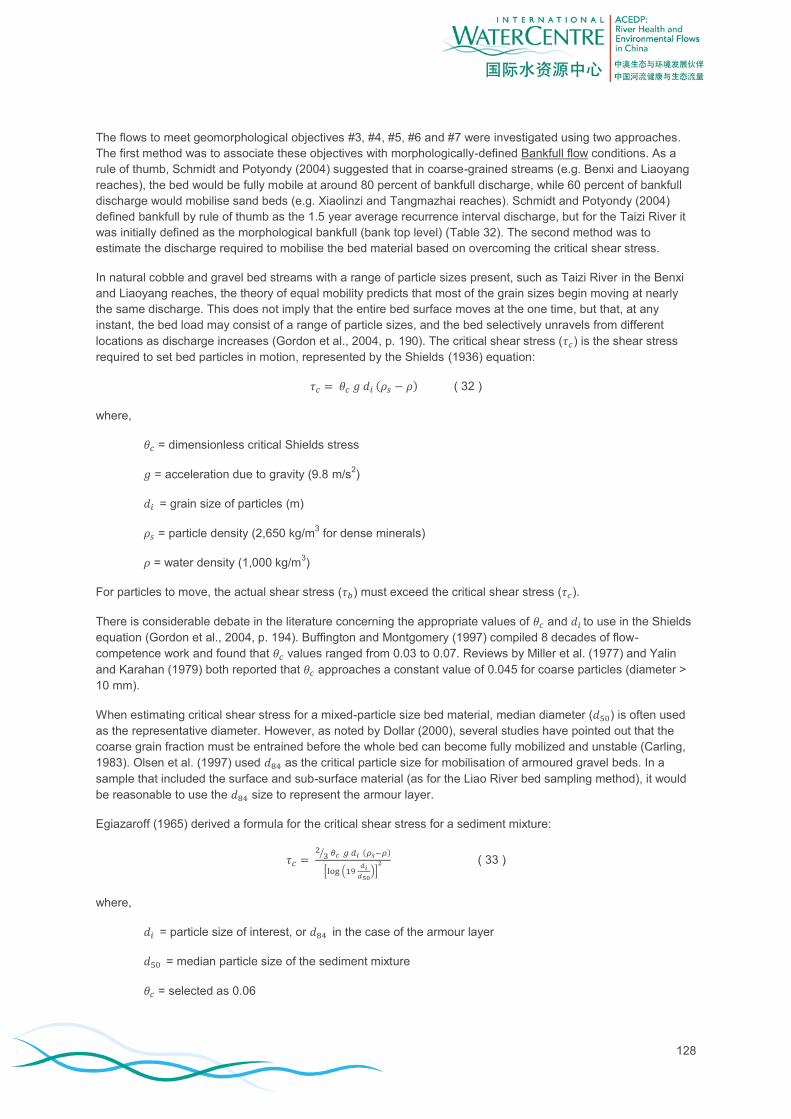
128

The flows to meet geomorphological objectives #3, #4, #5, #6 and #7 were investigated using two approaches.

The first method was to associate these objectives with morphologically-defined Bankfull flow conditions. As a

rule of thumb, Schmidt and Potyondy (2004) suggested that in coarse-grained streams (e.g. Benxi and Liaoyang

reaches), the bed would be fully mobile at around 80 percent of bankfull discharge, while 60 percent of bankfull

discharge would mobilise sand beds (e.g. Xiaolinzi and Tangmazhai reaches). Schmidt and Potyondy (2004)

defined bankfull by rule of thumb as the 1.5 year average recurrence interval discharge, but for the Taizi River it

was initially defined as the morphological bankfull (bank top level) (Table 32). The second method was to

estimate the discharge required to mobilise the bed material based on overcoming the critical shear stress.

In natural cobble and gravel bed streams with a range of particle sizes present, such as Taizi River in the Benxi

and Liaoyang reaches, the theory of equal mobility predicts that most of the grain sizes begin moving at nearly

the same discharge. This does not imply that the entire bed surface moves at the one time, but that, at any

instant, the bed load may consist of a range of particle sizes, and the bed selectively unravels from different

locations as discharge increases (Gordon et al., 2004, p. 190). The critical shear stress ( ) is the shear stress

required to set bed particles in motion, represented by the Shields (1936) equation:

( 32 )

where,

= dimensionless critical Shields stress

= acceleration due to gravity (9.8 m/s2)

= grain size of particles (m)

= particle density (2,650 kg/m3 for dense minerals)

= water density (1,000 kg/m3)

For particles to move, the actual shear stress ( ) must exceed the critical shear stress ( ).

There is considerable debate in the literature concerning the appropriate values of and to use in the Shields

equation (Gordon et al., 2004, p. 194). Buffington and Montgomery (1997) compiled 8 decades of flow-

competence work and found that values ranged from 0.03 to 0.07. Reviews by Miller et al. (1977) and Yalin

and Karahan (1979) both reported that approaches a constant value of 0.045 for coarse particles (diameter >

10 mm).

When estimating critical shear stress for a mixed-particle size bed material, median diameter ( ) is often used

as the representative diameter. However, as noted by Dollar (2000), several studies have pointed out that the

coarse grain fraction must be entrained before the whole bed can become fully mobilized and unstable (Carling,

1983). Olsen et al. (1997) used as the critical particle size for mobilisation of armoured gravel beds. In a

sample that included the surface and sub-surface material (as for the Liao River bed sampling method), it would

be reasonable to use the size to represent the armour layer.

Egiazaroff (1965) derived a formula for the critical shear stress for a sediment mixture:

( 33 )

where,

= particle size of interest, or in the case of the armour layer

= median particle size of the sediment mixture

= selected as 0.06

129

Komar (1987) modified the original Shields entrainment expression to account for a natural mixed-particle size

bed, to derive the flow-competence equation:

( 34 )

where,

= the maximum diameter of the sediment mixture

= selected as 0.045

The exponent values 0.6 and 0.4 come from data obtained in streams where and particle

diameter ranges were 10 to 100 mm. When Lorang and Hauer (2003) applied the equation of Komar (1987) to 33

high gradient (≥ 0.002 m/m) gravel/cobble-bed ( = 35 - 1,000 mm) rivers in New Zealand [using data from

Hicks and Mason (1991)], they found that the value of 0.045 for the dimensionless critical Shields stress ( )

predicted that the beds of most streams would be stable at bankfull, and a more appropriate value of was 0.02.

This corresponds with the minimum value of suggested by Andrews (1983) for gravel-bed rivers.

Andrews (1983) estimated that the dimensionless critical Shields stress could be estimated by:

( 35 )

In this case, would be the statistic selected to represent the armour layer and is the median diameter of

the sub-surface layer.

Julien (1995) presented equations for critical shear stress that were a function of the angle of repose of the

particles ( ):

(for silts and sands) ( 36 )

(for gravels and cobbles) ( 37 )

where,

( 38 )

and where,

= specific gravity of the sediment

= kinematic viscosity of water (1 × 10-6

m2/s)

The above review suggests that there are at least five versions of the critical shear stress approach:

1. The original Shields (1936) equation [Eqn 30], selecting an appropriate value of

2. The modified Shields (1936) equation of Egiazaroff (1965) [Eqn 31]

3. The modified Shields (1936) equation of Komar (1987) [Eqn 32]

4. The original Shields (1936) equation [Eqn 30], calculating an appropriate value for using the equation

of Andrews (1983) [Eqn 32]

5. The equations of Julien (1995) [Eqn 34, Eqn 35 and Eqn 36]

As indicated above, the value of the dimensionless critical Shields stress ( ) covers a wide range, but based on

the experience of Lorang and Hauer (2003) and Andrews (1983), a value on the low end of the range (0.02) was

selected for application of the original Shields (1936) equation (method 1 above) in the Taizi River. The original

values of used by Egiazaroff (1965) and Komar (1987) were retained for methods 2 and 3 above. The

sediment was assumed to have a specific gravity of 2.65.

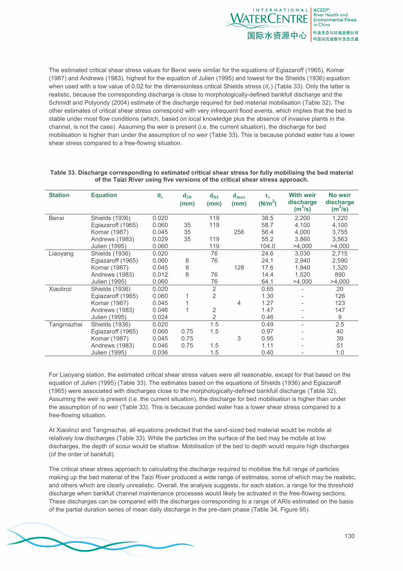
130

The estimated critical shear stress values for Benxi were similar for the equations of Egiazaroff (1965), Komar

(1987) and Andrews (1983), highest for the equation of Julien (1995) and lowest for the Shields (1936) equation

when used with a low value of 0.02 for the dimensionless critical Shields stress ( ) (Table 33). Only the latter is

realistic, because the corresponding discharge is close to morphologically-defined bankfull discharge and the

Schmidt and Potyondy (2004) estimate of the discharge required for bed material mobilisation (Table 32). The

other estimates of critical shear stress correspond with very infrequent flood events, which implies that the bed is

stable under most flow conditions (which, based on local knowledge plus the absence of invasive plants in the

channel, is not the case). Assuming the weir is present (i.e. the current situation), the discharge for bed

mobilisation is higher than under the assumption of no weir (Table 33). This is because ponded water has a lower

shear stress compared to a free-flowing situation.

Table 33. Discharge corresponding to estimated critical shear stress for fully mobilising the bed material of the Taizi River using five versions of the critical shear stress approach.

Station Equation

(mm)

(mm)

(mm)

(N/m2)

With weir discharge

(m3/s)

No weir discharge

(m3/s)

Benxi Shields (1936) 0.020 119 38.5 2,200 1,220 Egiazaroff (1965) 0.060 35 119 58.7 4,100 4,100 Komar (1987) 0.045 35 256 56.4 4,000 3,755 Andrews (1983) 0.029 35 119 55.2 3,860 3,563 Julien (1995) 0.060 119 104.0 >4,000 >4,000

Liaoyang Shields (1936) 0.020 76 24.6 3,030 2,715 Egiazaroff (1965) 0.060 8 76 24.1 2,940 2,590 Komar (1987) 0.045 8 128 17.6 1,940 1,320 Andrews (1983) 0.012 8 76 14.4 1,520 890 Julien (1995) 0.060 76 64.1 >4,000 >4,000

Xiaolinzi Shields (1936) 0.020 2 0.65 - 20 Egiazaroff (1965) 0.060 1 2 1.30 - 126 Komar (1987) 0.045 1 4 1.27 - 123 Andrews (1983) 0.046 1 2 1.47 - 147 Julien (1995) 0.024 2 0.46 - 9

Tangmazhai Shields (1936) 0.020 1.5 0.49 - 2.5 Egiazaroff (1965) 0.060 0.75 1.5 0.97 - 40 Komar (1987) 0.045 0.75 3 0.95 - 39 Andrews (1983) 0.046 0.75 1.5 1.11 - 51 Julien (1995) 0.036 1.5 0.40 - 1.0

For Liaoyang station, the estimated critical shear stress values were all reasonable, except for that based on the

equation of Julien (1995) (Table 33). The estimates based on the equations of Shields (1936) and Egiazaroff

(1965) were associated with discharges close to the morphologically-defined bankfull discharge (Table 32).

Assuming the weir is present (i.e. the current situation), the discharge for bed mobilisation is higher than under

the assumption of no weir (Table 33). This is because ponded water has a lower shear stress compared to a

free-flowing situation.

At Xiaolinzi and Tangmazhai, all equations predicted that the sand-sized bed material would be mobile at

relatively low discharges (Table 33). While the particles on the surface of the bed may be mobile at low

discharges, the depth of scour would be shallow. Mobilisation of the bed to depth would require high discharges

(of the order of bankfull).

The critical shear stress approach to calculating the discharge required to mobilise the full range of particles

making up the bed material of the Taizi River produced a wide range of estimates, some of which may be realistic,

and others which are clearly unrealistic. Overall, the analysis suggests, for each station, a range for the threshold

discharge when bankfull channel maintenance processes would likely be activated in the free-flowing sections.

These discharges can be compared with the discharges corresponding to a range of ARIs estimated on the basis

of the partial duration series of mean daily discharge in the pre-dam phase (Table 34, Figure 95).

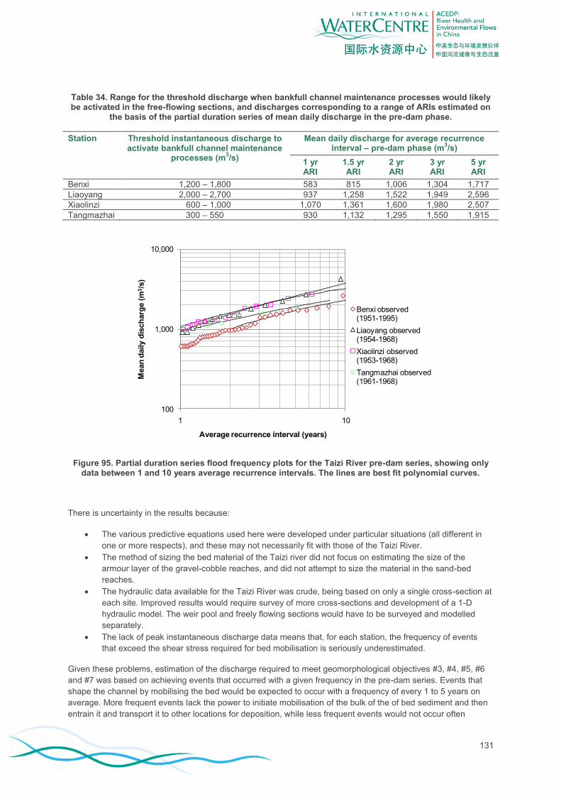
131

Table 34. Range for the threshold discharge when bankfull channel maintenance processes would likely be activated in the free-flowing sections, and discharges corresponding to a range of ARIs estimated on

the basis of the partial duration series of mean daily discharge in the pre-dam phase.

Station Threshold instantaneous discharge to activate bankfull channel maintenance

processes (m3/s)

Mean daily discharge for average recurrence interval – pre-dam phase (m

3/s)

1 yr ARI

1.5 yr ARI

2 yr ARI

3 yr ARI

5 yr ARI

Benxi 1,200 – 1,800 583 815 1,006 1,304 1,717

Liaoyang 2,000 – 2,700 937 1,258 1,522 1,949 2,596

Xiaolinzi 600 – 1,000 1,070 1,361 1,600 1,980 2,507

Tangmazhai 300 – 550 930 1,132 1,295 1,550 1,915

Figure 95. Partial duration series flood frequency plots for the Taizi River pre-dam series, showing only data between 1 and 10 years average recurrence intervals. The lines are best fit polynomial curves.

There is uncertainty in the results because:

The various predictive equations used here were developed under particular situations (all different in

one or more respects), and these may not necessarily fit with those of the Taizi River.

The method of sizing the bed material of the Taizi river did not focus on estimating the size of the

armour layer of the gravel-cobble reaches, and did not attempt to size the material in the sand-bed

reaches.

The hydraulic data available for the Taizi River was crude, being based on only a single cross-section at

each site. Improved results would require survey of more cross-sections and development of a 1-D

hydraulic model. The weir pool and freely flowing sections would have to be surveyed and modelled

separately.

The lack of peak instantaneous discharge data means that, for each station, the frequency of events

that exceed the shear stress required for bed mobilisation is seriously underestimated.

Given these problems, estimation of the discharge required to meet geomorphological objectives #3, #4, #5, #6

and #7 was based on achieving events that occurred with a given frequency in the pre-dam series. Events that

shape the channel by mobilising the bed would be expected to occur with a frequency of every 1 to 5 years on

average. More frequent events lack the power to initiate mobilisation of the bulk of the of bed sediment and then

entrain it and transport it to other locations for deposition, while less frequent events would not occur often

100

1,000

10,000

1 10

Mean

daily d

isch

arg

e (

m3/s

)

Average recurrence interval (years)

Benxi observed (1951-1995)

Liaoyang observed (1954-1968)

Xiaolinzi observed (1953-1968)

Tangmazhai observed (1961-1968)

132

enough to be the major control over channel form. These larger events may periodically reset the channel form,

but more frequent events do the bulk of the work over time. If regular (say, every 1 to 5 years) events with the

capacity to mobilise bed material are removed from the flow regime by dam regulation, the channel will likely be

colonised by vegetation (Petts, 1979; Petts and Gurnell, 2005). For the Taizi River, a key problem remains – the

lack of peak instantaneous discharge data to characterise the flood frequency.

There is only one event on the Taizi River for which the instantaneous peak discharge is published. On 5 August

1960, at Liaoyang, the instantaneous peak was 18,100 m3/s (JICA, 2000), and flow records indicate a

corresponding mean daily discharge of 5,820 m3/s, giving a ratio of 3.1. In a study of the Jiaojiang River system

in Zhejiang province, Gippel et al. (2009a) found that the peak discharge was between 1.5 and 3 times higher

than the mean daily discharge, with the factor decreasing in the downstream direction. For Benxi and Liaoyang

stations, the 1.5 year ARI event (expressed as mean daily discharge), when factored by 1.5 to 3, fitted within the

range of bankfull channel maintenance discharge estimated on the basis of morphological bankfull and shear

stress to mobilise bed material (Table 34). At Xiaolinzi and Tangmazhai the natural morphological bankfull (Table

32) is much smaller than the peak discharge likely to be associated with the 1.5 year ARI event (Table 34). This

could be because the channel has aggraded with sand since regulation (due to reduced frequency of floods with

the capacity to scour and transport sediment), or it could be that these lowland reaches naturally had a relatively

small channel and flooded more frequently than upstream reaches. This is not an unusual phenomenon (e.g.

Nanson and Young, 1981; Pickup and Marks, 2001). Nanson and Young (1981) commented that:

“This decrease in channel size apparently results from a sudden decline in channel slope and

associated stream power, the cohesive nature of downstream alluvium, its retention on the channel

banks by a dense cover of pasture grasses, and the availability of an extensive floodplain to carry

displaced floodwater. Under these conditions floodwaters very frequently spill out over the floodplain

and the downstream channel-flow becomes a relatively unimportant component of the total peak

discharge. This emphasizes the importance of these floodplains as a part of the total channel system.”

Thus, there is a suggestion in the data that prior to regulation by dams and construction of flood dikes, the Taizi

River in the Xiaolinzi and Tangmazhai reaches was characterised by frequent inundation, and this was likely to

have carried ecological significance.

Given the uncertainties, the rule of thumb of Schmidt and Potyondy (2004) was applied as a reasonable first

estimate of the discharge required to meet geomorphological objectives #3, #4, #5, #6 and #7 (those associated

with bankfull processes). The estimate was based on factoring the 1.5 year ARI event ( ) by 0.8 at Benxi and

Liaoyang, and 0.6 at Xiaolinzi and Tangmazhai. This gave discharges of 652 m3/s at Benxi, 1,006 m

3/s at

Liaoyang, 817 m3/s at Xiaolinzi and 679 m

3/s at Tangmazhai. The Tangmazhai value was reduced to 540 m

3/s –

the natural morphological bankfull discharge ( ) (Table 32) – because bankfull-related geomorphic

processes do not increase much in intensity as the river exceeds bankfull level. It is stressed that these are

specified as mean daily discharges; these magnitudes may not mobilise all fractions of the bed sediments at

Benxi and Liaoyang, but in reality, these mean daily discharges would be associated with much higher

instantaneous peak discharges that would mobilised the bed sediments.

Geomorphological objective #6 is concerned with maintaining pool and riffle morphology. Pool-riffle morphology

reflects a significant aspect of channel adjustment, so pools and riffles often manifest as stable channel forms

(e.g. Carling, 1991; Powell, 2009, p. 357; White et al., 2010). Thus, assuming a stable channel alignment, the

positions of pools and riffles tend to remain approximately in the same place. In gravel and cobble bed rivers (i.e.

the Benxi and Liaoyang reaches), mobilisation of most size fractions of the bed material would likely be an

important part of the process to maintain the pool-riffle morphology, but the minimum required duration of bed

material mobilisation for each channel forming event is not known. However, it would likely be in the order of

hours or days rather than weeks or months. In the low flow intervals between channel forming events the pool

and riffle morphology persists because the flows are incompetent to transport sufficient bed material to scour the

riffle crests and fill the pools. Sand-bed rivers (i.e. the Xiaolinzi and Tangmazhai reaches) differ significantly,

because in the low flow intervals between channel forming events the flow may be competent to re-distribute at

least the finer fraction of the bed material from the higher velocity zones to the low velocity (pool) zones. This

would have the effect of reducing pool depths over the time between pool scouring events.

133

The Taizi River appears to have alternate bar morphology for at least part of its length from Beisha River junction

to the Hun River junction (Figure 61, Figure 96). Alternate bars are not apparent on aerial photographs upstream

of Beisha River junction, where the bed material is cobble-gravel size (also, the channel upstream of Beisha

River junction is highly modified by hard lining, weirs, and gravel extraction). The alternate bars begin

immediately downstream of the junction of the Beisha River, a northern tributary which supplies sand to the river,

and which would also make a significant contribution to the discharge.

Figure 96. Taizi River downstream of Beisha River junction and just upstream of Xiaolinzi, showing alternating bar morphology. Image from Google maps.

Alternate bars are attached to alternate banks of the channel and slope downwards towards the other bank, so

that the deepest point (pool centre) is normally found across the channel from the centre of the bar. Alternate bar

morphology should not be confused with pool-riffle morphology. At low flow, if the pools alternate from bank to

bank, then the morphology is alternate bars rather than pool-riffle (Keller, 1972). While a high width-depth ratio

appears to favour formation of alternate bars, it can cross an order of magnitude (12 to >100), and other

geomorphic factors such as degree of meandering, channel slope and grain size and distribution are important.

As a general rule, alternate bars are favoured in wide, straight and relatively steep channels, with sand or gravel

bedload. Of course, the bars will not form without suitable hydrodynamic (flow) conditions. The empirical work

has tended to focus on morphology rather than formative processes, but it is interesting to note that alternate

bars have been observed in parts of the world where the rivers are fed by snowmelt, or where the flow regime

has regular spring runoff (Gippel, 2002). Welford (1994) conducted a field test of Tubino’s (1991) nonlinear model

on a U.S. river and found that alternate bar formation frequently occurred during hydrologic conditions that did not

conform to all of the assumptions of the theory. Despite these problems, Welford (1994) confirmed the notions

that bar formation occurs on the falling limb of a hydrograph, is dependent on a critical width-depth ratio, and

there is a lag between flow variability and bar form response. General models of upper and lower limits of

alternate bar formation were presented by Jaeggi (1984), Chang (1984) and Chang (1988). These models are

based on critical Shields stress, boundary shear stress, sediment properties, channel dimensions and energy

slope. Ikeda (1983; 1984) presented a model that predicted alternate bar wavelength on the basis of flow velocity,

sediment properties, channel dimensions and energy slope.

Gippel (2002) found that the development and persistence of alternate bars in the lower Snowy River, Australia,

seemed to require an extended period of ideal conditions (moderate magnitude, long duration spring snowmelt

event), while the bars did not appear for a number of years following a large flood event. The studies of alternate

bar formation suggest that channel forming flows of long-duration (weeks to months, including recession) are

required. Also, the coefficient of variation of annual flows is low (< 0.5) in places with persistent alternate bars

(Welford, 1984). A high coefficient of variation of annual flows implies highly variable flood magnitudes from year

to year, which means in some years the floods are too small to create the bar morphology and in other years the

134

floods are large enough that they break down the bar morphology. At the four Taizi gauging stations the CV of

annual flow was less than 0.5 in the pre-Shenwo and post-Guanyinge phases, but greater than 0.5 in the post-

Shenwo/pre-Guanyinge phase.

In the Tangmazhai and Xiaolinzi reaches of the Taizi River the duration of the pre-regulation high flow season

spells exceeding the threshold for sand mobilisation was of the order of weeks and months (Figure 74, Figure 75,

Figure 76, Figure 77 and Table 33). In the post-dam phases the duration reduced markedly to the order of days

(Figure 74, Figure 75, Figure 76 and Figure 77). The impact of this hydrological change on alternate bar

morphology has not been examined in the Taizi River. In fact, nothing has been documented on the location,

history, formation, or ecological significance of alternate bar morphology on the Taizi River.

At this stage there is insufficient information available to allow formulation of a specific recommendation on the

flows required to maintain alternate bar morphology in the lower Taizi River. However, as a general principle, the

flows identified for bankfull channel maintenance would likely be adequate to form the alternate bar morphology,

provided the recession rate lies within the natural bounds (i.e. is not too rapid).

Geomorphological objective #4 concerns prevention of the establishment of mature vegetation that could lead to

channel contraction, by binding the bed sediments and offering low velocity zones for increased deposition of

sediment. There are three main groups of vegetation that are usually considered in this context: trees and shrubs,

grasses, and macrophytes. Trees, shrubs and grasses generally colonise the riparian areas and edges, and

would tend to migrate towards the centre of the channel under a reduced flow regime. Macrophytes are rooted

aquatic plants that can be emergent, submergent, or floating. Macrophytes provide cover for fish and substrate

for aquatic invertebrates and act as food for some fish (Carpenter and Lodge, 1986; Caffrey et al., 1999).

However, if not regularly kept in check they can colonise the stream channel, reducing the availability of other

habitat types, such as deep and fast water, and clean gravel and cobble substrate, and also lowering dissolved

oxygen levels at night (see Caffrey et al., 1999). Guscio et al (1965) reported reductions in the design channel

capacity of up to 97 percent in a channel choked with macrophytes.

In the Liaohe, the riparian vegetation is dominated by a range of herb communities, including large emergent

macrophytes such as Typha spp. and Phragmites spp. and the large submergent macrophyte

Potamogetonaceae (CRAES, 2010). Floating macrophytes were reported by CRAES (2010) to be uncommon. In

the riparian zone of the Liaohe main stem, dense communities of trees and shrubs occur in patches where the

river abuts steep valley walls (in the Benxi reach). Elsewhere, the riparian zone is virtually devoid of trees,

presumably because of removal by humans for various reasons such as firewood collection, clearing access to

the river, cultivation to the river banks, and disturbance by sand and gravel extraction. These activities may

regularly keep macrophyte growth in check in some places, but it is worthwhile to consider control of

macrophytes by flow.

Macrophyte growth is a function of numerous factors, but water flow is known to be a prime factor (Franklin et al.,

2008). The effects of flow on macrophytes are usually considered in terms of the hydrological regime (frequency

of disturbance and duration of stable flow conditions) and velocity (which is associated with mechanical damage

and uprooting). Long periods of stable baseflow may encourage invasion by macrophytes; for example, in

Australia, Typha spp. are associated with stable water levels typical of regulated rivers (Mackay and Marsh,

2005). Riis and Biggs (2003) found that significant macrophyte development in New Zealand rivers was restricted

to streams which experienced an average of less than 13 flood events per year (i.e. events exceeding 7 times the

median discharge magnitude). In sandy substrates, the important flood events may be of a lower magnitude than

this (Riis et al., 2008). Periods of low flow can also keep macrophytes in check (Franklin et al., 2008). Both the

abundance and diversity of macrophytes are stimulated at low to medium velocities, with growth being restricted

at higher velocities (Madsen et al., 2001). Roberts and Ludwig (1991) found a relationship between the zonation

of emergent species and the strength of current and wave action and a gradual change in the plant community

along the velocity gradient. Riis and Biggs (2003) found that macrophyte abundance peaked in the velocity range

0.3 – 0.5 m/s. Chambers et al. (1991) suggested 1 m/s as an upper limit of velocity, above which macrophytes

are few or absent. The flexible stems and leaves of Potamogeton crispus reduce the frontal area exposed to flow

so it has a high tolerance to hydraulic stress and is found in slow to fast-flowing water (Mackay and Marsh, 2005).

Based on similarity of growth forms, information in the literature, and field observations, Mackay and Marsh (2005)

rated Scirpus acutus (tule – a giant species of sedge in the plant family Cyperaceae) and Schoenoplectus validus

(river club rush – a native plant of Australia) as having moderate resistance to hydraulic disturbance. The linear

135

leaves of Typha spp. would be expected to reduce drag, but longer leaves would experience higher drag than

shorter leaves, so Mackay and Marsh (2005) rated Typha spp, slightly lower in resistance to hydraulic

disturbance than Schoenoplectus validus. In an area of the Tone River, Japan, with maximum velocities of 0.8 –

0.9 m/s, Asaeda et al. (2005) observed that the depths at which Typha angustifolia (0.4 – 0.7 m) and Zizania

latifolia (0.4 – 0.6 m) grew overlapped, while the velocity in both zones was generally < 0.8 m/s. Phragmites

australis zones were relatively shallower (mostly < 0.3 m) and had low velocity (< 0.4 m/s).

Chemical and mechanical control methods are often deployed to prevent infestation of channels by macrophytes

(Franklin et al., 2008), however natural hydrodynamic controls can obviate the need for such interventions (Duan

et al., 2002). Groeneveld and French (1995) found that colonisation of channels by Scirpus acutus (tule) could be

prevented if flow events of sufficient water velocity and depth were delivered. They showed that sufficient

bending stress induced by hydrodynamic drag on the macrophyte stem caused stem rupture – failure involving

permanent deformation and loss of plant function. They quantified the depth-velocity envelope required to induce

rupture, providing a means to estimate the flow required to provide hydrodynamic protection against

encroachment by macrophytes.

In the Taizi River, the discharge required to rupture macrophyte stems was computed by application of

Groeneveld and French’s (1995) relationship. The diameter of the macrophyte stems was set, as recommended

by Groenveld and French (1995), to 11.9 mm. A threshold was then evaluated to give a 95 percent chance of

stem rupture (this allowed some macrophytes to remain in the channel for seasonal re-colonisation). The

threshold was reported as the discharge required for the product of flow depth (D) and velocity (V) to exceed 0.52.

Depth and velocity were assumed to be cross-section means. While the relationship of Groeneveld and French

(1995) is specific to Scirpus acutus, it would be expected to apply to robust macrophytes with moderate

resistance to hydraulic stress such as Typha spp. Potamogeton spp. would be expected to have a higher

tolerance to hydraulic stress, while Phragmites spp. would be expected to have a lower tolerance to hydraulic

stress. Given that Chambers (1991) reported few if any macrophytes were found in waters with velocities

exceeding 1 m/s, this was included as an additional criterion. A further criterion was included to ensure that the

majority of the channel bed was impacted by this flow component; the wetted perimeter ( ) should be at least

equal to 80% of the wetted perimeter corresponding to the median baseflow in August (the month of highest

baseflow) ( ). Thus, the minimum discharge for checking macrophyte invasion in the Taizi River was

the lowest of that determined by V = 1 m/s and V . D = 0.52, with the condition that . For the

four stations, the limiting criterion in each case was V . D = 0.52. This gave threshold discharges of 77 m3/s at

Benxi, 140 m3/s at Liaoyang, 101 m

3/s at Xiaolinzi and 63 m

3/s at Tangmazhai.

Geomorphological objectives #1 and #2 are concerned with removal of fine sediment from the surface of the

stream bed. These objectives apply to pools and riffles, or wherever it is important for ecological reasons to

maintain a bed surface clean of fines. Sediment-entrainment theories can be used to predict the mobilisation of

unconsolidated surface deposits on the bed (silt- and sand-sized). These sediments might accumulate during

long periods of low flow. It is normally assumed that fine particles will be flushed out when the threshold of motion

for some percentage of the particles is reached. One method of predicting when particles will become entrained

in the flow is based on the Hjulström curves, which relate particle size to mean velocity required for erosion,

deposition and transportation (Gordon et al 2004 p.192). The critical velocity (in m/s) for initiation of sediment

movement (for particles >1 mm diameter) is , where is the median particle diameter in

millimetres. The Hjulström curve also predicts the limits for erosion of fine sands down to clay size sediment, and

these values can be read from the curve (Gordon et al 2004, p. 192). The velocity near the bed ( ) is predicted

by , where is the mean channel velocity (Gordon et al 2004, p. 193). The bed surface material will

become unstable when .

Estimates of the discharge required to initiate movement of fine surface accumulations in the Taizi River were

made based on the assumption that the material covered the size range coarse silt up to fine sand at Benxi and

Liaoyang (where the native bed material is cobble- and gravel-size), and coarse silt at Xiaolinzi and Tangmazhai

(where the native bed material is sand-size). This assumes that clay- and fine silt-sized material either remains in

suspension or forms flocs of organic/mineral/biological material that are not finer than coarse silt. These materials

are entrained at mean channel velocities greater than 0.4 m/s. This is a conservative estimate, as much of the

surface material is flocs of organic/mineral/biological material that is lower in density than mineral material, so it

would be more easily entrained than mineral material. The criteria gave discharges of 28 m3/s (with weir) and

136

15 m3/s (no weir) at Benxi, 125 m

3/s (with weir) and 15 m

3/s (no weir) at Liaoyang, 23 m

3/s at Xiaolinzi and

73 m3/s at Tangmazhai.

The final geomorphological-flow relationship is concerned with provision of adequate water in the vertical (depth)

and the horizontal (wetted perimeter) dimensions of the cross-section at times of baseflow. The gauging station

cross-sections available for the Taizi River were not selected for the purpose of analysis of critical hydraulic

habitat availability; it is not known how typical they are of the reaches that they represent, or if they represent

pools or shallow areas. Thus, applying hydraulic habitat criteria to these cross-sections is an uncertain

procedure. An alternative is to establish a tentative rule of thumb based on expert opinion that sets a limit on

maximum reduction in wetted perimeter and depth compared to the conditions that prevailed prior to regulation

by dams.

There is usually a distinct difference in the size of the sediment making up the bed and banks, a steepening of

the slope on the banks, and presence of vegetation on the banks. The bed is the habitat for benthic animals, and

because of its relatively low cross-river gradient (compared to the banks) the area of bed under water is relatively

sensitive to changes in stage height. The toe of the banks (edge of bed) identified by the minimum value of the

slope of the relationship between wetted perimeter and stage height was found to correspond closely with the

stage height of the median August (highest flow month) baseflow. So, the latter index ( ) was used to

define the maximum extent of the channel bed.

Bartschi (1976) suggested that a 20% reduction in wetted perimeter at mean flow might be the maximum

allowable to maintain aquatic health. Applying this maximum 20% allowable reduction in wetted perimeter rule to

the median baseflow for each month (Figure 97) suggested a minimum baseflow (Table 35) that could be

recommended in the absence of an alternative, more compelling, hydraulic criterion. The basis of this rule is that

while a 20% reduction in the area of wet channel bed will reduce habitat availability, the impact on river health is

considered tolerable2. This rule applies only to cross-sections at riffles, or pool crossings, because at times of low

flow these are the hydraulic controls of the water width at pools.

Water depth is important in pools, riffles and pool crossings. Large-bodied fish normally need pool depths of the

order of 1 m or more (for swimming space, cover, and avoidance of thermal stress in shallow water summer).

Fish also need adequate water depths (of the order of 0.2 m or greater) at the thalweg through shallow areas to

enable movement and migration. Benthic invertebrates require a water depth in the order of 0.1 m or greater.

These hydraulic criteria can be evaluated if a range of pool and riffle cross-sections are available. With multiple

cross-sections, the discharge that satisfies the objective is computed from the cross-section where the hydraulic

criterion is most limited (as the criterion will then be satisfied at all cross-sections). Multiple cross-sections were

not available for the Taizi River, so a rule of thumb was used to set the maximum allowable reduction in suitable

depth habitat relative to what was available under the pre-dam hydrological regime. Suitable depth habitat was

defined as the width of channel where depth was at least as deep as two thresholds: 0.1 m and 0.2 m. Following

the same arbitrary rule that was applied to wetted perimeter reduction, a 20% reduction in width of suitable depth

habitat (at riffles or pool crossings) at median baseflow was the maximum allowable to maintain aquatic health

(Figure 98). Applying this rule (for two depth criteria) to the median baseflow for each month suggested a

minimum baseflow (Table 36 and Table 37) that could be recommended in the absence of an alternative, more

compelling, hydraulic criterion.

It is interesting to note that reducing the wetted perimeter by 20% gave rise to an average (for the months of the

year) reduction in baseflow discharge of 45% at Benxi, 58% at Liaoyang, 50% at Xiaolinzi and 90% at

Tangmazhai. Reducing the width of channel with depth ≥ 0.1 m by 20% gave rise to an average (for the months

of the year) reduction in baseflow discharge of 38% at Benxi, 56% at Liaoyang, 44% at Xiaolinzi and 95% at

Tangmazhai. Reducing the width of channel with depth ≥ 0.2 m by 20% gave rise to an average (for the months

of the year) reduction in baseflow discharge of 33% at Benxi, 53% at Liaoyang, 44% at Xiaolinzi and 96% at

Tangmazhai. The large allowable reduction in discharge at Tangmazhai comes about from the very flat nature of

the morphology of the bed of the lower part of the channel combined with very low downstream gradient. This

highlights the sensitivity of hydraulic habitat analysis to the channel morphology. The use of only one cross-

2 Note that there are no local data from the Taizi River to support this assumption; it is based on expert opinion

only, and is intended as a starting point that should be investigated further.

137

section gives an uncertain result. Also, because the analysis focuses on the lowest part of the channel, which

may not be very wide, it is important to survey the bed of the channel to a high level of detail.

Figure 97. Illustration of method of calculating discharge corresponding to 20% reduction in wetted perimeter at pre-dam median baseflow discharge. Not drawn to scale.

Figure 98. Illustration of method of calculating discharge corresponding to 20% reduction in width of channel with depth ≥ 0.1 m at pre-dam median baseflow discharge. The same method was used to

calculate the discharge corresponding to 20% reduction in width of channel with depth ≥ 0.2 m. Not drawn to scale.

Wetted perimeter at pre-dam median baseflow

80% of wetted perimeter at pre-dam median baseflow

𝑾 %

Width with D ≥ 0.1 m at pre-dam median baseflow

80% of width with D ≥ 0.1 m at pre-dam median baseflow

0.1 m

0.1 m

𝑫 . , %

138

Table 35. Median baseflow discharge (m3/s) for each month and computed discharge (m

3/s) that provides

80% of the wetted perimeter that is available at the median natural baseflow.

Benxi Liaoyang Xiaolinzi Tangmazhai

Jan 3.7 2.2 7.9 2.9 8.9 4.2 9.3 1.0

Feb 3.8 2.3 7.3 2.6 8.5 3.8 8.6 1.0

Mar 4.0 2.4 9.1 3.5 12.2 6.2 10.8 1.0

Apr 8.7 7.7 19.6 8.3 21.2 12.6 19.4 1.0

May 20.8 11.7 17.9 7.6 19.2 11.8 20.0 1.0

Jun 17.3 8.7 9.2 3.5 11.1 5.8 18.6 1.0

Jul 23.5 12.6 33.5 14.0 39.2 14.2 17.1 1.0

Aug 38.6 18.1 58.6 53.3 55.4 48.0 65.3 16.9

Sep 26.0 14.1 41.2 17.4 44.2 17.3 45.3 14.4

Oct 15.1 8.1 33.4 14.0 40.2 14.3 33.2 12.6

Nov 11.1 7.9 23.0 9.7 29.5 13.4 31.0 12.3

Dec 5.6 3.3 10.4 4.1 15.2 8.5 16.1 1.0


3/s) that provides

80% of the width with water depth ≥ 0.1 m that is available at the median natural baseflow.


Jan 3.7 2.2 7.9 3.1 8.9 5.2 9.3 0.5

Feb 3.8 2.4 7.3 2.8 8.5 4.8 8.6 0.5

Mar 4.0 2.5 9.1 3.7 12.2 6.9 10.8 0.5

Apr 8.7 6.5 19.6 9.0 21.2 12.2 19.4 0.5

May 20.8 12.2 17.9 8.2 19.2 10.3 20.0 0.5

Jun 17.3 11.2 9.2 3.8 11.1 6.4 18.6 0.5

Jul 23.5 13.0 33.5 15.0 39.2 17.5 17.1 0.5

Aug 38.6 21.7 58.6 53.0 55.4 51.6 65.3 20.6

Sep 26.0 15.5 41.2 18.2 44.2 18.0 45.3 18.0

Oct 15.1 11.0 33.4 14.9 40.2 17.6 33.2 16.4

Nov 11.1 9.6 23.0 10.5 29.5 16.5 31.0 7.9

Dec 5.6 3.6 10.4 4.4 15.2 8.0 16.1 0.5


3/s) that provides

80% of the width with water depth ≥ 0.2 m that is available at the median natural baseflow.


Jan 3.7 2.4 7.9 3.4 8.9 5.6 9.3 0.6

Feb 3.8 2.5 7.3 3.2 8.5 5.3 8.6 0.6

Mar 4.0 2.6 9.1 4.0 12.2 7.5 10.8 0.6

Apr 8.7 6.5 19.6 9.5 21.2 10.9 19.4 0.6

May 20.8 16.5 17.9 8.6 19.2 9.8 20.0 0.6

Jun 17.3 15.8 9.2 4.1 11.1 7.0 18.6 0.6

Jul 23.5 16.8 33.5 16.0 39.2 21.4 17.1 0.6

Aug 38.6 23.8 58.6 56.2 55.4 24.2 65.3 24.4

Sep 26.0 17.2 41.2 19.4 44.2 22.3 45.3 22.8

Oct 15.1 10.5 33.4 15.9 40.2 21.6 33.2 1.1

Nov 11.1 7.6 23.0 11.3 29.5 16.9 31.0 0.6

Dec 5.6 3.6 10.4 4.7 15.2 8.6 16.1 0.6

139

Development of vegetation flow objectives The riparian vegetation of the Tazi River catchment was sampled in 120 quadrats in Sep-Oct 2009 (CRAES,

2010). Of a total of 156 species recorded, Bidens biternata was by far the most common. This is a widespread

plant, native to Liaoning. Of the aquatic plants, Polygonum hydropiper (marsh pepper smartweed) was the most

common.

In the Sep-Oct 2009 sampling, the main community types of riparian herb included Bidens biternata community,

Artemisia community, Scirpus community, Echinochloa crusgalli community, Rumex acetosa community,

Potentilla chinensis community, Rorippa community and Zoysia community. In wet areas, Polygonum community

and Cyperus community are widely distributed, while Phragmites community, Typha community and Oenanthe

javanica (Chinese celery) community were rare (CRAES, 2010).

The Sep-Oct 2009 survey sampled aquatic macrophytes from three tributaries of the Taizi River, namely, north

arm of Taizi River, Xi River and Haicheng River. Eight large submergent plants were found, belonging to

Potamogetonaceae family (Potamogeton crispus, Potamogeton pusillus, Potamogeton malatanus, Potamogeton

pectinatus), Trapa bispinosa, Ceratophyllum demersum, Hydrilla verticillata and Myriophyllum spicatum. Floating

leaved plants were not found in the quadrats but were occasionally seen on the edge of the river (CRAES, 2010).

The Sep-Oct 2009 field survey found that in most streams of the Taizi River catchment, the riparian vegetation

was degraded, reduced in size, or absent, with much of the riparian land being reclaimed for farming (CRAES,

2010). Thus, it is important to protect remaining vegetation communities, and to encourage rehabilitation in

degraded areas. This requires effort on two fronts, the first being local management to prevent degradation and

encourage rehabilitation (through regulations, physical barriers and re-planting), and the second to provide a

pattern of flows that is matched to the life cycle of the riparian plant communities.

Flow-vegetation relationships have not been seriously investigated in the Taizi River catchment. While it is likely

that particular flow levels are required at certain times of the year to support particular plant communities, there is

no information available on which to base such specific objectives. For this reason, generic flow objectives were

developed to support the plant communities.

Watering the plant communities at the toe of the bank was regarded as high priority, because a vegetated toe

offers physical protection to the bank from scour at times of high flow, and because there is a reasonable chance

that the lower bank has some intact vegetation (i.e. the lower bank is not utilised for farming). Flowing water in

the channel maintains the water table level so that soil moisture is available on the lower bank. The main growth

period is May to June and the main flowering and fruiting period is July to September. Thus, a low flow pulse is

required in the March to May period to increase soil moisture of the lower bank. The pulse should at least fully

inundate the channel bed, so the minimum flow magnitude was set equal to the maximum wetted perimeter,

which was equivalent to the wetted perimeter of the median baseflow in August in the pre-dam phase

( ). Bartschi’s (1976) maximum 20% allowable reduction in wetted perimeter rule was applied to the

median baseflow for each month in the pre-dam phase to set the low flow and high flow components (baseflows).

This rule maintains 80 percent of the wetted perimeter of the median baseflow in each month in the pre-dam

phase ( ). The main objective of these flow components is to maintain the groundwater gradient at

times when the stream is losing to groundwater, thereby ensuring a source of water to the riparian zone.

Another priority was seed dispersal, which is achieved by a high flow pulse in the September to November period

following the flowering and fruiting season. Seed is sourced from the bank vegetation and, for some plants, may

require inundation to dislodge seeds (Moggridge and Gurnell, 2010). Given limited knowledge of the distribution

of the vegetation assets and the modes of seed dispersal, here an arbitrary criterion of achieving the full bed

width ( ) was applied. The effectiveness of this flow relies on the seeds being blown, or dropping,

onto the bed. This flow magnitude is suggested as a starting point for evaluation. It is possible that flows higher

than those suggested will play an important role in plant propagule dispersion, as found by Moggridge and

Gurnell (2010).

The other priority for vegetation was the remnant wetland communities that occur in the Xiaolinzi and

Tangmazhai reaches, although these are not abundant and have not been mapped. Also, the lower floodplain

has been alienated from the river by dikes constructed close to the edge of the river channel. Inundation of the

140

floodplain requires exceeding the level of the bank top, which was set here to be equal to the morphological bank

top ( ) plus 0.1 m depth. The timing of the event was set to the normal flood season of July to November.

Development of fish flow objectives The fish communities of the Taizi River catchment were recently sampled on two occasions in May and October

2009, finding a total of 42 species belonging to 12 families (CRAES, 2010). Cyprinidae species accounted for 53%

of total species, Gobiidae was ranked next with 13% and Cobitidae was ranked third with 11%. Cyprinidae

species were dominant in abundance, accounting for 69% of the total fish catch.

Phoxinus lagowskii Dybowski (Lagowski’s minnow) was the dominant fish species in Taizi River catchment

(CRAES, 2010). It was present in 43 percent of all sampling points. Also widely distributed were Abbottina

rivularis, Pseudorasbora parva and Cobitidae misgurnus anguillicaudatus, Nemacheilus nudus and Cobitis

granoci.

Potentially threatened species in the Taizi River catchment are Hypomesus olidus (pond smelt), Perccottus

glehni Dybowski and Cottus poecilopus. These fish species have been recorded many times historically, but are

now seen only occasionally. The abundances of Odontobutis obscura, Huigobio chinssuensis, Lefua costata,

Squalidus chankaensis Dybowski, Squalidus sihuensis and Oryzias latipes (medaka) have decreased greatly in

historical times (CRAES, 2010). Some species recorded in the historical data, such as Coilia ectenes and Hucho

taimen were not recorded in the 2009 survey (CRAES, 2010).

Rare, protected fishes of high conservation value sampled in the Taizi River catchment were Lampetra morii Berg,

Hypseleotris swinhonis, and Huigobio chinssuensis, Odontobutis obscura, Perccottus glehni Dybowski, Squalidus

chankaensis Dybowski and Squalidus sihuensis (CRAES, 2010). CRAES (2010) provided some limited

information on the preferred and tolerable habitat and life cycles of these seven species. This information was

supplemented with data from www.fishbase.org/, www.loaches.com/, www.geochembio.com/,

www.iucnredlist.org/, www.fao.org/fishery, http://el.erdc.usace.army.mil, http://fl.biology.usgs.gov and other

published sources, and then combined with data for the five other species that were listed (see above) by

CRAES (2010) as potentially threatened, or previously recorded. As Cyprinidae was the dominant family in the

2009 survey (CRAES, 2010), which was also the observation of Li and Xu (1995) for the Liaohe, relevant

information on some common representatives of that family (Cyprinus carpio, Ctenopharyngodon idellus and

Hypophthalmichthys nobilis) was also included (Appendix A). The potential spawning periods for the selected

species crossed the range February to October, but most species spawned within the period April to July (Figure

99).

Figure 99. Potential spawning periods for key fish species in the Taizi River. Data from various sources (see Appendix A).

1 2 3 4 5 6 7 8 9 10 11 12

Lampetra morii

Odontobutis obscura

Huigobio chinssuensis

Perccottus glehni

Hypseleotris swinhonis

Squalidus chankaensis

Squalidus sihuensis

Hypomesus olidus

Cottus poecilopus

Lefua costata

Oryzias latipes

Coilia ectenes

Hucho taimen

Cyprinus carpio carpio

Ctenopharyngodon idellus

Hypophthalmichthys nobilis

Potential spawning months

No spawning migration

Potamodromous

Anadromous

http://www.fishbase.org/

http://www.loaches.com/

http://www.geochembio.com/

http://www.iucnredlist.org/

http://www.fao.org/fishery

http://el.erdc.usace.army.mil/

http://fl.biology.usgs.gov/

141

On the basis of the known needs of the fish species present in the river system, particularly the fish of high

conservation value (Appendix A), a number of fish-flow objectives were formulated. For some of these species

there were no known flow-ecology relationships that could be used to derive specific flow objectives. Due to the

sparsity of information about the tolerable and preferred depth and velocities, some of the hydraulic criteria were

generic in nature. The chosen velocity and depth limits are intended only as a starting point for evaluation of the

flow requirements of fish.

For the Taizi River, it was assumed that cease to flow was not desirable for fish health, except for short periods at

Liaoyang (where cease to flow occurred naturally). Critical discharge for low flow and high flow components (i.e.

baseflows) was defined on the basis of depth and width criteria. The critical hydraulic criterion for fish that reside

in pools was assumed to be 0.1 m minimum depth over riffles and pool crossings, based on the assumption that

pools are maintained by flow at shallow points (the hydraulic control points). Bartschi’s (1976) maximum 20%

allowable reduction in habitat rule was applied to each month to the width of channel with depth ≥ 0.1 m at pre-

dam median baseflow discharge (Figure 98 and Table 36). The critical hydraulic criterion for fish that reside in

riffles and pool crossings was assumed to be 0.2 m minimum depth. This was decided on the basis of expert

opinion, and is not meant to be a widely applicable generic criterion. Bartschi’s (1976) maximum 20% allowable

reduction in habitat rule was applied to each month to the width of channel with depth ≥ 0.2 m at pre-dam median

baseflow discharge (Figure 98 and Table 37). These depth criteria ensured the availability of a reasonable area

of minimum desirable water depth for pool and riffle habitats separately. The adopted minimum flow was then the

largest of the two calculated flows.

A low flow pulse was included to allow potamodromous fish periods of free local movement during the lowest flow

months (December to April). A minimum depth was chosen at riffles and pool crossings that would cause a

significant rise in water level from the normal baseflow level. These depths were considered appropriate for the

particular cross-sections available for the Taizi River mainstem, and should not be considered generic criteria for

application elsewhere.

Low flow pulses were also required to stimulate spawning. Not all fish species are stimulated to spawn by a rise

in discharge, some requiring water temperature to rise to a certain range. The upstream spawning migration of

the anadromous species such as Coilia ectenes, and perhaps Hypomesus olidus, is associated with a rise in

discharge prior to the spawning season proper. The timing of a suitable rise in discharge for C. ectenes would be

March to May, and for H. olidus February to April. The upstream migration of C. ectenes is reported to require a

maximum velocity of 1 m/s (Jiang et al., 2010). The spawning of C. ectenes requires a high velocity High flow

pulse in the period June to August.

Of the potamodromous species, spawning of Cyprinus carpio carpio appears to be associated with a rise in

discharge in the April to May period through the association with lowered ionic concentration of the water, while

Ctenopharyngodon idellus and Hypophthalmichthys nobilis require a sustained rise in discharge to stimulate and

then maintain spawning in the period April to July. A rise in discharge closer to the high flow season would have a

greater change of sustaining the spawning, so a High flow pulse with sufficiently high velocity in the June to July

period was considered appropriate.

The spawning of some fish species (Perccottus glehni, Hypseleotris swinhonis, Hypomesus olidus, Cottus

poecilopus, Lefua costata, Oryzias latipes and Cyprinus carpio carpio) takes place off the main channel, in

backwaters, littoral zones and connected lakes. For these species, the main requirement is that such areas are

present, and then inundated during the spawning period. In the Taizi River, much of the channel is hard-lined,

channelized and diked, so a limitation on the spawning of these species could be the availability and accessibility

of such physical habitat, rather than suitability of the flow regime per se. Provision of winter baseflow (High flow

component), plus a sustained High flow pulse of 2 weeks over the period April to July, was considered desirable

for spawning for this group of species.

Development of macroinvertebrate flow objectives Macroinvertebrates were sampled in the Taizi River in May 2009 at 210 quadrats; a total of 131 species were

recorded (CRAES, 2010). The previous research on macroinvertebrates in the Taizi has focused on the

relationship between macroinvertebrate distribution and water pollution levels (CRAES, 2010), so information on

Taizi-specific macroinvertebrate-flow relationships is unavailable. For this reason, generic flow objectives were

developed to support the macroinvertebrate communities.

142

Old and Acreman (2006) reviewed the literature concerning the flow requirements of macroinvertebrates, and

only the findings (i.e. not the information sources) are referred to here. The basic findings were that:

River flow, temperature and the composition and stability of the substratum are the three dominant

variables controlling macroinvertebrate distribution and survival.

Many invertebrate species require specific substrate types and assemblages may change in response to

the deposition of fine sediment on the channel bed.

Periodic flushing (from flow pulses) is desirable to prevent settling of fines clogging interstitial spaces in

the substratum.

A artificially constant flow regime, in excess of natural low flows, results in enhanced numbers or

biomass of macroinvertebrates, even when short-term fluctuations are imposed.

Where flows are reduced and constant, there is a tendency for an increase in deposit feeding

invertebrates and a reduction in grazers; also, Diptera, Olichoptera and Ephemeroptera may be

enhanced or reduced and Plecoptera are usually severely reduced.

A narrower range of environmental conditions and increased flow stability can lead to a dynamically

fragile macroinvertebrate community, which is susceptible to flow event disturbances because it has

developed in their absence.

Constant flows below the natural flow may result in severe reductions in wetted area and hence

reduction in overall productivity of the stream.

The results of the stream bed drying up even for short periods can be catastrophic, although some

species can survive in pools and under rocks for short periods.

A detrimental flow regime is one with substantial intermittent flow variations, such as ramping for

hydropower generation, periodically exposing large areas of channel and leaving species stranded

Macroinvertebrates are resilient to high flows and recover over time periods shorter than the generation

times of most species. Macroinvertebrates also show resilience to droughts.

The study by Armitage and Ladle (1991) of velocity and depth preferences for 5 invertebrate species

(stoneflies Leuctra fusca and Isoperla grammatical; caddis-fly Polycentropus flavomaculatus and

Rhyacophila dorsalis; and pea mussel Sphaerium corneum) found that occurrence was generally higher

for all species in the lowest depth class (0 – 25 cm) but preferences for velocity and substrate particle

size was species specific.

Many of the FLOWS environmental flow assessments conducted in Victoria, Australia use a depth greater than

0.1 m as a desirable attribute for macroinvertebrates. Some studies are referred to by Cottingham et al. (2005),

and two examples of other studies that used this criterion are Doeg (2004) and Wealands et al. (2007). The use

of this criterion in FLOWS studies possibly originates from its use in the first full application of the FLOWS

method by Loddon River Environmental Flows Scientific Panel (2002). In that study the criterion was applied to

the shallowest point on the thalweg in a reach, such that if satisfied, the entire thalweg would have a depth

greater than 0.1 m. The later study of Wealands et al. (2007) applied this criterion differently, as the median

depth at riffle and run cross-sections. The Victorian Environmental Flows Monitoring and Assessment Program

(VEFMAP) adopted as two of the key sub-hypotheses for the habitat processes and macroinvertebrates

conceptual model: [for the low flow period] “Do implemented environmental flows maintain adequate area and

depth of at least 0.1 m in shallow, slow water and riffle/run habitats?” [and, for the high flow period] “Do

implemented environmental flows increase area of riffle and/or run habitat?” (Chee et al., 2006). Thus, Chee et al.

(2006) acknowledged the value of the 0.1 m minimum depth criterion for maintaining habitat for

macroinvertebrates, but they also recognised the need for an “adequate area” of such habitat in the low flow

period, and that this area should be greater in the high flow period.

Although none of the FLOWS-related studies mentioned above documented their justification for the minimum

0.1 m depth criterion, it is based on the idea that, as a minimum, macroinvertebrates require a cover of some

water on their habitat (the bed), and that in cobble and gravel-bed streams a flow depth of 0.1 m will cover most

of the protruding stones [But, note that for some insects, protruding stones are required for egg deposition

(Lancaster et al., 2003; Lancaster and Downes, 2010)]. Application of this criterion (assuming it is reasonable)

will ensure the availability of some suitable habitat for macroinvertebrates. However, when it is applied as the

minimum depth on the thalweg, or as the median depth at shallow cross-sections, then there will be a large

percentage of the bed with a water depth less than 0.1 m, which is presumably less than ideal, and perhaps

unsuitable, for some or many species of macroinvertebrate. The FLOWS studies have concentrated on providing

143

macroinvertebrate habitat at riffles, so it is relevant to note that Cottingham et al. (2003) defined riffles as areas

with coarse substrate, fast flow, turbulent flow at the surface, and a depth of < 0.3 m. This depth criterion was

based on the need for enough light to reach the bed to allow primary production (i.e. the penetration depth of

photosynthetically active radiation) and the Froude number exceeding 0.18. In this case an upper depth was

defined because the regulated summer flows (irrigation water supply) of the river under investigation, the

Goulburn River, had drowned out most of the riffle habitat, and this criterion was intended to restore it by

reducing summer flows.

For the Taizi River, it was assumed that cease to flow was not desirable for macroinvertebrate health, except for

short periods at Liaoyang (where cease to flow occurred naturally). Critical discharge for low flow and high flow

components (i.e. baseflows) was defined on the basis of depth and wetted perimeter criteria. The critical

minimum depth for macroinvertebrates was assumed to be 0.1 m. Bartschi’s (1976) maximum 20% allowable

reduction in habitat rule was applied to each month to the width of channel with depth ≥ 0.1 m at pre-dam median

baseflow discharge (Figure 98 and Table 36). The same allowable habitat reduction rule was applied to wetted

perimeter (Figure 97 and Table 35). The depth criterion ensured the availability of a reasonable area of minimum

desirable water depth, and the wetted perimeter rule ensured the availability of a reasonable area of bed covered

by water (regardless of depth). The adopted minimum flow was then the largest of the two calculated flows. A

maximum criterion was also applied to baseflows in the spring and summer months of March to August (the

period with highest potential for primary production). Due to lack of information about euphotic depth and the

hydraulics of riffles in the Taizi River, the maximum baseflow was based on the pre-dam monthly distribution of

baseflow. The arbitrarily selected statistic was the 98th percentile baseflow discharge (baseflow equalled or

exceeded 2 percent of the time) ( ) (Table 38). The intention of this rule was to limit long periods of unnaturally

high flows in the warmer months that would drown out riffles and pool crossings. This objective was not intended

to prevent spring-summer flow pulses, which might be beneficial for macroinvertebrates.

Table 38. 98th

percentile baseflow discharge (m3/s) for each month of spring and summer in the pre-dam phase.

98th

percentile baseflow discharge in the pre-dam phase ( ) (m3/s)


March 11.3 22.2 29.1 25.7

April 40.5 42.6 40.3 24.4

May 60.8 50.3 44.7 46.8

June 60.6 96.9 58.0 38.0

July 81.9 131.5 98.4 119.1

August 189.2 321.1 197.0 200.4

A low flow pulse was deemed important for flushing the hyporheia, in order to maintain water quality. The

hydraulic requirements for flushing the hyporheia are not known, but as a minimum the bed would have to be

covered by water. Here it was assumed that fully inundating the bed at riffles or pool crossings would create a

hydraulic gradient that would force an exchange of water through the hyporheia (equivalent to ). This

magnitude is suggested as a starting point for evaluation. Research such as that undertaken by Hancock and

Boulton (2005) is required in order to properly define the appropriate magnitude of flows for flushing the

hyporheia.

The floodplain also provides habitat for macroinvertebrates. Thus, an overbank flow was recommended for the

high flow season, but only for Xiaolinzi and Tangmazhai reaches, where floodplain wetlands are present.

The requirements for flushing fine sediment from the bed, and occasionally mobilising bed sediments, were

recognised in the geomorphological flow objectives.

Comprehensive flow objectives A comprehensive list of objectives was compiled for each of the geomorphological (Table 39), vegetation (Table

40), fish (Table 41) and macroinvertebrate (Table 42) ecosystem categories.

144

Table 39. Geomorphological flow objectives.

ID Objective Flow component

Hydraulic criteria (V = mean velocity; D = mean depth; WP = wetted perimeter; Q = discharge; = minimum of…)

Mean annual frequency/ duration


Timing Reach

1a Flush fine sediment from surface of beda Low flow

pulse m s 2 per year /

1 day each 3 in 5 years Feb-

Jun All

1b Control macrophyte expansion that could lead to channel contraction

b

Low flow pulse

m s ,

and

1 per year / 1 day

4 in 5 years Dec-Jun

All

1c Control macrophyte expansion that could lead to channel contraction

b

High flow pulse

m s ,

and

1 per year / 1 day

4 in 5 years Jul-Nov

All

1d Maintain diversity and dynamism of channel form (width, depth, bars, bank shape, etc); mobilise bed sediments; erode banks; scour sand from pools

c

Bankfull 80% of (Benxi and Liaoyang);

60% of (Xiaolinzi); (natural) (Tangmazhai);

recession rate within natural range

≤1 per year / 1 day


All

a. During the spring, it is important to remove the fine surface sediment after the ice has melted to maintain a clean surface and sub-surface for utilisation by benthic

invertebrates and benthic fish.

b. The required frequency of macrophyte control pulses is not known. Two per year on average is suggested as a starting point for evaluation.

c. Recommended for natural high flow season so that high flows do not interfere with the spawning and migration processes of other seasons.

145

Table 40. Vegetation flow objectives.

ID Objective Flow component

Hydraulic criteria (WP = wetted perimeter; Q = discharge)



Timing Reach

2a Increase bank toe soil moisture

a

Low flow pulse

1 per year / 3 days

4 in 5 years Mar-May

All

2b Maintain groundwater gradient

Low flow Continuous > 75% of time Mar-Jun

All

2c Maintain groundwater gradient

High flow Continuous > 75% of time Jul-Nov All

2d Disperse seedb High flow

pulse 1 per year /

1 day 4 in 5 years Sep-

Nov All

2e Maintain floodplain wetland communities

Overbank m depth ≤1 per year / 1 day

2 in 5 years Jul-Nov Xiaolinzi and Tangmazhai

a. Three days is suggested as the duration to allow time for water seep through the bed and bank material. Actual required duration depends on hydraulic conductivity of

the bed and bank material. Three days duration is suggested as a starting point for evaluation.

b. One day duration should be sufficient to disperse seed; rate of fall within natural range is important to allow seed to settle at different levels.

c. Recommended for natural high flow season so that high flows do not interfere with the spawning and migration processes of other seasons. The bankfull flow

magnitude is set by the bank top, and should take dikes into account. Exceeding the bank top level by 0.1 m is intended to cause spill of water to the floodplain.

146

Table 41. Fish flow objectives.

ID Objective Relevant guild and example species

Flow component

Hydraulic criteria (V = mean velocity; D = mean depth; WP = wetted perimeter; Q = discharge)



Timing Reach

3a Prevent habitat loss through bed drying, prevent deterioration of water quality

Pool guild and riffle guild

Cease-to-flow

m3s ≤ 1 spell per year / ≤ 16 days/yr (Liaoyang); no cease to flow in other reaches

5 in 5 years

All year

All

3b Maintain sufficient water depth in pools for large bodied fish

a

Pool guild; C. idellus and C. carpio carpio

Low flow 0 1m Continuous > 75% of time

Dec-Jun

All

3c Maintain sufficient width of adequate depth at riffles and pool crossings

Riffle guild Low flow 0 2m Continuous > 75% of time

Dec-Jun

All

3d Allow a period of free local movement of resident fish during the lowest flow months

b

Potamodromous guild Low flow pulse

m Benxi m Liaoyang m Xiaolinzi m Tangmazhai over high points in thalweg

1 per year / 14 days

4 in 5 years

Dec-Apr

All

3e Stimulate upstream spawning migration of C. ectenes; maintain longitudinal connectivity

b

C. ectenes Low flow pulse

m Liaoyang m Xiaolinzi m Tangmazhai over high points in thalweg; m s

1 per year / 14 days

4 in 5 years

Mar-May

Liaoyang, Xiaolinzi, and Tangmazhai

147


Flow component




Timing Reach

3f Stimulate upstream spawning migration of H. olidus; maintain longitudinal connectivity

b

H. olidus Low flow pulse

m Xiaolinzi m Tangmazhai over high points in thalweg; m s

1 per year / 7 days

4 in 5 years

Feb-Apr

Xiaolinzi, Tangmazhai

3g Maintain sufficient water depth in pools for large bodied fish

Pool guild High flow 0 1m Continuous > 75% of time

Jul-Nov

All

3h Maintain sufficient width of adequate depth at riffles and pool crossings

Riffle guild High flow 0 2m 80% Continuous > 75% of time

Jul-Nov

All

3i Stimulate and maintain spawning, then facilitate downstream transport of semi-buoyant eggs within the water column

c

C. idellus, H. nobilis High flow pulse

0 7 1 9 m s 1 per year / 5 days

4 in 5 years

Jun-Jul

All

3j Spawning opportunity for spp. requiring access to low velocity zones off the main channel; also stimulate spawning of H. taimen

b

P. glehni, H. swinhonis, H. olidus, C. poecilopus, L. costata, O. latipes, C. carpio carpio; H. taimen

High flow pulse

m Benxi m Liaoyang m Xiaolinzi m Tangmazhai over high points in thalweg

1 per year / 5 days

4 in 5 years

Apr-Jul

All

3k Spawning of C. ectenes

d

C. ectenes High flow pulse

0 7 1 4 m s; m

1 per year / 5 days

4 in 5 years

Jun-Aug

Liaoyang, Xiaolinzi and Tangmazhai

148


Flow component




Timing Reach

3l Provide access to floodplain habitat between inner and outer dikes, and flush food and organic matter from floodplain

e

All species, especially those that require access to floodplains for spawning or rearing

Overbank m depth ≤1 per year / 1 day

2 in 5 years

Jul-Nov

Xiaolinzi and Tangmazhai

a. The criterion assumes pool levels are maintained by having flow at riffles and pool crossings (i.e. the hydraulic control points).

b. These depth criteria are specific to the cross-sections available at these locations and should not be considered generic criteria for application elsewhere. The depths

are adequate to cause a significant rise in water level from the normal baseflow level. The durations are suggested as a starting point for evaluation. Note that

C. ectenes cannot migrate upstream of Shenwo dam.

c. The velocity range criterion is from the literature. This range of velocity is less typical of Xiaolinzi and Tangmazhai (the downstream destination of the eggs) than at

Benxi and Liaoyang. The duration of 5 days is suggested as a starting point for evaluation.

d. The velocity range criterion is from the literature. C. ectenes also requires suitable spawning grounds, the availability of which is uncertain the Taizi River. Note that

C. ectenes cannot migrate upstream of Shenwo dam.

e. Recommended for natural high flow season so that high flows do not interfere with the spawning and migration processes of other seasons. The bankfull flow


149

Table 42. Macroinvertebrate flow objectives.


Flow component

Hydraulic criteria (D = mean depth; WP = wetted perimeter; Q = discharge)



Timing Reach

4a Prevent habitat loss through drying of riffles and pool crossings

Riffle guild Cease-to-flow

m3s ≤ 1 spell per year / ≤ 16 days/yr (Liaoyang); no cease to flow elsewhere

5 in 5 year All year

All

4b Maintain appropriate depth over riffles and pool crossings

Riffle and pool guild, Gammarus spp., Gastropoda sp.

Low flow 0 1m ;

Continuous > 75% of time

Dec-Jun

All

4c Maintenance of reasonable area of wet bed

Riffle and pool guild Low flow Continuous > 75% of time

Dec-Jun

All

4d Flushing to maintain water quality of hyporheia

a

Hyporheic guild, Baetis spp., Cheumatopsyche spp.

Low flow pulse

2 per year / 1 day

4 in 5 years Dec-Jun

Benxi and Liaoyang

4e Maintain appropriate depth over riffles and pool crossings

Riffle and pool guild, Gammarus spp., Gastropoda sp.

High flow 0 1m ;

Continuous > 75% of time

Jul-Nov

All

4f Maintenance of reasonable area of wet bed

Riffle and pool guild, Odonata spp. (dragonfly), and Diptera spp. (true fly)

High flow Continuous > 75% of time

Jul-Nov

All

4g Provide access to floodplain habitat between inner and outer dikes

b

Floodplain/wetland guild Overbank m depth ≤1 per year / 1 day


Xiaolinzi and Tangmazhai

a. The hydraulic requirement for flushing the hyporehia was not known. As a starting point for evaluation, it was assumed that fully inundating the bed at riffles or pool

crossings would create a hydraulic gradient that would force an exchange of water through the hyporheia.

b. Recommended for natural high flow season so that high flows do not interfere with the spawning and migration processes of other seasons. The bankfull flow


150

Flow magnitudes associated with the flow objectives The hydraulic criteria were evaluated at each site for each of the objectives in each ecosystem category. This

evaluation produced an estimate of the flow magnitude required to meet each objective (Table 43, Table 44,

Table 45 and Table 46).

Evaluation of the hydraulic and hydrological criteria Each objective was evaluated for each site using the available flow time series. As the flow event objectives were

specified in multi-dimensional terms of magnitude, duration, annual frequency and inter-annual frequency, a

sophisticated form of spells analysis was undertaken to determine the compliance of each of the flow

components. This method of compliance analysis was first documented by Gippel et al. (2009b). Compliance

means the frequency that components appeared in the flow regime, relative to the frequency required to achieve

the agreed level of river health (i.e. the standard determined by the environmental flows assessment). The final

score for each year was based on water year (beginning in December), not calendar year.

Table 43. Benxi flow components, and their magnitudes, annual frequencies and event durations. Magnitudes in m

3/s. Flow magnitudes, frequencies and durations are minimums, unless specified. G =

geomorphological, V = vegetation, F = fish, M = macroinvertebrates. CTF = cease to flow, LF = low flow, LFP = low flow pulse, HF = high flow, HFP = high flow pulse, BF = bankfull, OB = overbank.

Categ-

ory

Flow

component

Objective

ID Jan Feb Mar Apr May Jun Jul Aug Sep Oct Nov Dec

G LFP 1a

G LFP 1b

G HFP 1c

G BF 1d

V LFP 2a

V LF 2b 2.4 7.7 11.7 8.7

V HF 2c 12.6 18.1 14.1 8.1 7.9

V HFP 2d

V OB 2e

F CTF 3a

F LF 3b 2.2 2.4 2.5 6.5 12.2 11.2 3.6

F LF 3c 2.4 2.5 2.6 6.5 16.5 15.8 3.6

F LFP 3d

F LFP 3e

F LFP 3f

F HF 3g 13.0 21.7 15.5 11.0 9.6

F HF 3h 16.8 23.8 17.2 10.5 7.6

F HFP 3i

F HFP 3j

F HFP 3k

F OB 3l

M CTF 4a

M LF 4b 2.2 2.4 2.5-11.4 6.5-40.5 12.2-60.8 11.2-60.6 3.6

M LF 4c 2.2 2.3 2.4 7.7 11.7 8.7 3.3

M LFP 4d

M HF 4e 13.0-81.9 21.7-189.2 15.5 11.0 9.6

M HF 4f 12.6 18.1 14.1 8.1 7.9

M OB 4g

87.0; 1/yr; 5 d

15 riffle; 28 pool; 2/yr; 1 d

77 ; 1/yr; 1 d

77 ; 1/yr; 1 d

38.6 ; 1/yr; 3 d

38.6 ; 1/yr; 1 d

652 ; 1/yr; 1 d

not applicable

not applicable

not applicable

not applicable

≤ 0.01; never

≤ 0.01; never

38.6 ; 2/yr; 1 d

not applicable

11.4; 1/yr; 14 d

not applicable

80.3 - 912; 1/yr; 5 d

151

Table 44. Liaoyang flow components, and their magnitudes, annual frequencies and event durations. Magnitudes in m



Event independence is an important consideration in determining event frequency and duration. If, following a

flood peak, the biota are still in a highly disturbed state, or the intended ecological process has been completed,

when a subsequent flood peak occurs, then the peaks could not be considered ecologically independent. In

general, a larger impact on the biota and the physical environment would be expected the higher the magnitude

of the event, so a longer recovery time would be expected for large events compared to small events. Thus, it is

reasonable to assume that the length of the interval for event independence should increase with the discharge

magnitude. Here, independence was based on two criteria. First, following a rule similar to that of Beard (1974),

the flow must fall to less than 75 percent of the flow threshold before the next independent event begins. Second,

events should be separated by a minimum number of days, set as a function of the magnitude of the discharge

threshold.

Following the recommendation of NRM South (2009), the maximum interval was arbitrarily set to 30 days, and

this applied to bankfull magnitude, which for this exercise was defined by the pre-dam 1.5 year ARI event ( )

(partial duration series). The minimum interval for event independence was arbitrarily set to 4 days. The length of

the interval for independence ( ), in whole days, for any discharge threshold ( ) was then determined by a

relationship, the non-linear nature of which was based on expert opinion:

( 39 )

( 40 )

Categ-

ory

Flow

component

Objective


G LFP 1a

G LFP 1b

G HFP 1c

G BF 1d

V LFP 2a

V LF 2b 3.5 8.3 7.6 3.5

V HF 2c 14.0 53.3 17.4 14.0 9.7

V HFP 2d

V OB 2e

F CTF 3a

F LF 3b 3.1 2.8 3.7 9.0 8.2 3.8 4.4

F LF 3c 3.4 3.2 4.0 9.5 8.6 4.1 4.7

F LFP 3d

F LFP 3e

F LFP 3f

F HF 3g 15.0 53.0 18.2 14.9 10.5

F HF 3h 16.0 56.2 19.4 15.9 11.3

F HFP 3i

F HFP 3j

F HFP 3k

F OB 3l

M CTF 4a

M LF 4b 3.1 2.8 3.7-22.2 9.0-42.6 8.2-50.3 3.8-96.9 4.4

M LF 4c 2.9 2.6 3.5 8.3 7.6 3.5 4.1

M LFP 4d

M HF 4e 15.0-131.5 53.0-321.1 18.2 14.9 10.5

M HF 4f 14.0 53.3 17.4 14.0 9.7

M OB 4g

not applicable

not applicable

84.5; 1/yr; 5 d

245 - 1180; 1/yr; 5 d

not applicable

not applicable

15 riffle; 125 pool; 2/yr; 1 d

140 ; 1/yr; 1 d

1006 ; 1/yr; 1 d

≤ 0.01; ≤ 1/yr; ≤ 16 d total duration per year

58.6 ; 2/yr; 1 d

140 ; 1/yr; 1 d

58.6 ; 1/yr; 3 d

58.6 ; 1/yr; 1 d

≤ 0.01; ≤ 1/yr; ≤ 16 d total duration per year

14.3; 1/yr; 14 d

14.3; 1/yr; 14 d

245 - 2225; 1/yr; 5 d

152

Table 45. Xiaolinzi flow components, and their magnitudes, annual frequencies and event durations. Magnitudes in m



Events were specified with a given minimum magnitude and duration, and the spells analysis isolated the

conforming events. This analysis produced a list of the number of complying events in each year, which was then

subjected to a test for the specified minimum annual frequency. Finally, a test for the specified inter-annual

frequency was applied. For this study, the inter-annual frequency test period was set to 5 years.3 Thus, for a

particular year, the number of complying years over a five year period (that year and the previous four years)

were counted and divided by 5 to give an average inter-annual frequency (i.e. a number that was 0.0, 0.2, 0.4,

0.6, 0.8 or 1.0). This is equivalent to the Observed (O). The Expected (E) is the specified inter-annual frequency,

i.e. 1, 2, 3, 4 or 5 events in 5 years (a number that was 0.2, 0.4, 0.6, 0.8 or 1.0). The hydrological score for each

year is then calculated as O/E. All values of O/E exceeding 1 were reduced to 1. Thus, the O/E score for any

particular year is not a measure of whether the event component occurred in that year, but a measure of how

often it occurred over that year and the previous 4 years, relative to the expectations for good river health. This

evaluation was applied separately to each event flow component that had a unique hydraulic/hydrologic

specification.

3 The period of 5 years was chosen using expert opinion, and is applicable only to this study. The compliance

method proposed here places no restriction on the length of the period over which inter-annual frequency of events is calculated, and the periods applied to events associated with each objective can be of different lengths.

Categ-

ory

Flow

component

Objective


G LFP 1a

G LFP 1b

G HFP 1c

G BF 1d

V LFP 2a

V LF 2b 6.2 12.6 11.8 5.8

V HF 2c 14.2 48.0 17.3 14.3 13.4

V HFP 2d

V OB 2e

F CTF 3a

F LF 3b 5.2 4.8 6.9-29.1 12.2-40.3 10.3-44.7 6.4-58.0 8.0

F LF 3c 5.6 5.3 7.5 10.9 9.8 7.0 8.6

F LFP 3d

F LFP 3e

F LFP 3f

F HF 3g 17.5 51.6 18.0 17.6 16.5

F HF 3h 21.4 24.2 22.3 21.6 16.9

F HFP 3i

F HFP 3j

F HFP 3k

F OB 3l

M CTF 4a

M LF 4b 5.2 4.8 6.9-29.1 12.2-40.3 10.3-44.7 6.4-58.0 8.0

M LF 4c 4.2 3.8 6.2 12.6 11.8 5.8 8.5

M LFP 4d

M HF 4e 17.5-98.4 51.6-197.0 18.0 17.6 16.5

M HF 4f 14.2 48.0 17.3 14.3 13.4

M OB 4g

985 (Nat); 2,761 (Curr); ≤1 yr; 1 d

251 - 1977; 1/yr; 5 d

251 - 4,000; 1/yr; 5 d

142.9; 1/yr; 5 d

25.7; 1/yr; 7 d

55.4 ; 1/yr; 3 d

55.4 ; 1/yr; 1 d

≤ 0.01; never

25.7; 1/yr; 14 d

25.7; 1/yr; 14 d

817 ; 1/yr; 1 d

23; 2/yr; 1 d

101 ; 1/yr; 1 d

101 ; 1/yr; 1 d

985 (Nat); 2,761 (Curr); ≤1 yr; 1 d

985 (Nat); 2,761 (Curr); ≤1 yr; 1 d

≤ 0.01; never

55.4 ; 2/yr; 1 d

153

Table 46. Tangmazhai flow components, and their magnitudes, annual frequencies and event durations. Magnitudes in m



The baseflow (Low flow and High flow components) criteria were evaluated differently to the method used for flow

events. For the Taizi River stations, the three different criteria used to define the Low flow and High flow

thresholds tended to produce very similar flow magnitudes, so the highest of the three estimates for each month

was adopted to satisfy all baseflow-related objectives. The flow series were then evaluated against these criteria,

for each month individually. This produced an annual time series for each month indicating the percentage of the

time that the flow exceeded the threshold. This is equivalent to the Observed (O). The Expected (E) was set to

75 percent of the time. This was based on the rationale that the index used to derive the median baseflow for

each month produced a similar value as the total flow exceeded 75 percent of the time (see Gippel et al., 2009a).

As the baseflow threshold for each month was set to allow a reduction of 20 percent of hydraulic habitat

compared to that provided by the median baseflow, then in the unimpacted scenario, baseflow would have to be

within Expected at least 75 percent of the time on average. The hydrological score for each month of each year

was then calculated as O/E. All values of O/E exceeding 1 were reduced to 1. A mean score for each of the low

flow season and the high flow season was then computed as the average O/E score for months December to

June and months July to November respectively. Unlike flow event components, the score for which was a

reflection of the hydrology over the previous five year period, baseflow components were evaluated for each year

individually. The rationale for this is that the ecological objectives dependent on baseflows describe responsive

processes. So, for example, it was assumed that macroinvertebrate health at any particular time is more a

reflection of the pattern of baseflows over the previous 12 months than the pattern of baseflows over the previous

5 years.4

4 This assumption is applicable only to this study. The compliance method proposed here places no restriction on

the length of the period over which inter-annual frequency of baseflow is calculated.

Categ-

ory

Flow

component

Objective


G LFP 1a

G LFP 1b

G HFP 1c

G BF 1d

V LFP 2a

V LF 2b 1.0 1.0 1.0 1.0

V HF 2c 1.0 16.9 14.4 12.6 12.3

V HFP 2d

V OB 2e

F CTF 3a

F LF 3b 0.5 0.5 0.5 0.5 0.5 0.5 0.5

F LF 3c 0.6 0.6 0.6 0.6 0.6 0.6 0.6

F LFP 3d

F LFP 3e

F LFP 3f

F HF 3g 0.5 20.6 18.0 16.4 7.9

F HF 3h 0.6 24.4 22.8 1.1 0.6

F HFP 3i

F HFP 3j

F HFP 3k

F OB 3l

M CTF 4a

M LF 4b 0.5 0.5 0.5-25.7 0.5-24.4 0.5-46.8 0.5-38.0 0.5

M LF 4c 1.0 1.0 1.0 1.0 1.0 1.0 1.0

M LFP 4d

M HF 4e 0.5-119.1 20.6-200.4 18.0 16.4 7.9

M HF 4f 1.0 16.9 14.4 12.6 12.3

M OB 4g

268 - 4000; 1/yr; 5 d

570 (Nat) / 883 (Curr); ≤1 yr; 1 d

65.3 ; 1/yr; 1 d

≤ 0.01; never

16.5; 1/yr; 14 d

16.5; 1/yr; 14 d

≤ 0.01; never

65.3 ; 2/yr; 1 d

16.5; 1/yr; 7 d

268 - 4000; 1/yr; 5 d

570 (Nat) / 883 (Curr); ≤1 yr; 1 d

88.7; 1/yr; 5 d

540 ; 1/yr; 1 d

570 (Nat) / 883 (Curr); ≤1 yr; 1 d

73; 2/yr; 1 d

63 ; 1/yr; 1 d

63 ; 1/yr; 1 d

65.3 ; 1/yr; 3 d

154

Rate of rise and rate of fall are characteristics of flow event components. It would be possible to apply these as

additional criteria when evaluating each flow component (along with duration, annual frequency and inter-annual

frequency). Putting aside the computational difficulty that would entail, it is of interest to know about the degree of

compliance to rise and fall thresholds separately to the relative compliance of events to frequency and duration

thresholds. Thus, rise and fall were evaluated independently of specific flow event components.

Rise and fall were evaluated for each month individually. First, a lower flow threshold was established for the

analysis – only considering flows exceeding the median baseflow for each month. Then, for rise and fall

separately, the total number of days in each month with rise (or fall) was counted, and the total number of days

exceeding the specified rise (or fall) thresholds (Table 28) was counted. These monthly totals were then summed

for the low flow season (Dec-Jun) and the high flow season (Jul-Nov). For each year, for these two seasons, for

both rise and fall, a ratio of number of days exceeding threshold to total number of days with rise (or fall) was

calculated. The ratio fell between zero and 1, with 1 signifying that all rises (or falls) exceeded the threshold, and

zero meaning that they were all under threshold. The score was then calculated as 1 minus the ratio, to give a

score from zero to 1 (100 percent of values less than threshold). This is equivalent to the Observed (O). The

Expected (E) was set as 75 percent of values less than threshold (because the threshold was based on the 75th

percentile of observed rates of rise and fall in the pre-dam flow series). The score was then calculated as O/E,

with all values of O/E exceeding 1 reduced to 1.

Results The evaluation produced a score ranging from 0 (distant from reference) to 1 (reference) for each flow

component for each year. The final reporting reduced these values down to a suite of core flow components

(Table 22):

– OB – Overbank

– BF – Bankfull

– HFP – High flow pulse

– HF – High flow

– LFP – Low flow pulse

– LF – Low flow

– CTF – Cease to flow

– HFF – High flow rate of fall

– HFR – High flow rate of rise

– LFF – Low flow rate of fall

– LFR – Low flow rate of rise

The components LFP and HFP had multiple sub-components that were evaluated individually. For each of the

LFP and HFP components, a combined score was calculated as the mean of the sub-component scores. There

was very little variation among the sub-component scores for any particular year, as the prevailing hydrological

conditions tended to impact similarly on all LFP, or all HFP sub-components.

Strictly speaking, rates of rise and fall are not discrete components, but are two of the characteristics of event

flow components. However, it was considered preferable to report on these characteristics separately, as they

are strongly linked to management of flow releases from dams.

An overall component score was calculated for each year as the lowest score of any component for that year. An

alternative approach to deriving an overall score is to average, or weight, the component scores. In combining

component scores it should be remembered that, from the perspective of river health, absence of high flow

components is not offset by the presence of low flow components, and vice-versa. This is consistent with the

philosophy of the natural flow paradigm. In this example of the Taizi River, the lowest score of the sub-indicators

was used as the overall score, but in the lower Yellow River a weighted averaging approach was used (Gippel et

al., 2012b).

155

Each score was reduced to one of five categories. The categories were: Very good is >0.8 – 1.0, Good is >0.6 –

0.8, Fair is >0.4 – 0.6, Poor is >0.2 – 0.4 and Critical is 0 – 0.2.5 For effective visual presentation, these

categories were represented by a colour scheme: Very good - blue, Good - green, Fair - yellow, Poor - orange,

and Critical – red.

High flow and Low flow component scores were calculated for each month (Figure 100), and these were then

averaged for the high flow season and low flow season to get an overall score for each year for each of these two

components. The baseflow component showed a degree of variability in the score during the pre-dam phases at

each site (Figure 100). Low scores arose in months with particularly high or low flows that fell outside the range

set for desirable river health. Flows in rivers are naturally variable, so this was an expected result. In an ideal

situation the “or natural” rule would be invoked for baseflow thresholds, and the pre-dam period would have

perfect compliance for every month. In the Taizi River application, the “or natural” rule was not used because it

was not possible to apply it to the post-dam phases (as natural flows were not modelled). Had it been possible,

application of the “or natural” rule would have improved the levels of compliance with baseflow objectives.

Most of the time in the pre-regulation phases the baseflows were in the good or moderate range (Figure 100).

Regulation at Benxi from Guanyinge dam did not have a major impact on baseflows from the perspective of river

health. The major change was March flows scoring poorly in most years after the dam began operation (Figure

100), which was due to dam releases being significantly higher than desirable in that month. August and

September also showed a decline in flow health (Figure 100), but due to a reduction in baseflows released from

the dam. At Lioayang and Xiaolinzi, baseflows were seriously impacted by regulation (Figure 100), which began

in 1969. June and July were the least affected months; August to April had reduced baseflows, and May had

much increased baseflows. The impact of regulation on baseflows was much less marked at Tangmazhai (Figure

100), mainly because the baseflow requirements for good river health were not as high (this was a function of the

morphology of the site). However, at Tangmazhai, regulation increased May flows beyond what was considered

appropriate for river good health (Figure 100).

As the IFH method encourages specification of flow component requirements at the level of species or guilds it

was possible to examine the time series of the favourability of flow conditions for species or guilds of particular

interest. For example, the anadromous species Coilia ectenes was once a valuable fishery resource of many

coastal rivers of China, including the Liao River system. This species was recorded in historical surveys of the

Taizi River, but it was not found in the 2009 survey (CRAES, 2010). C. ectenes is found in the lower and middle

reaches of river systems, so would not be expected in the Benxi reach. Like most fish species, the health of C.

ectenes populations is dependent on healthy physical form, vegetation, and macroinvertebrates, but C. ectenes

also has particular flow requirements associated with successful spawning. Focusing on the requirements of the

spawning cycle:

The upstream spawning migration is covered by objective is 3e (Table 41);

Spawning is covered by objective 3k (Table 41);

Transport of the eggs downstream is covered partly by objective 3k and partly by baseflow objectives 3g

and 3h (Table 41);

The entire spawning process involves upstream migration, spawning and downstream migration, which

potentially covers the period April to August, so baseflows over this period are also relevant, which are

covered by objectives 3b, 3c, 3g and 3h.

In the Taizi River regulation by Tanghe and Shenwo dams from 1969, and then by Guanyinge from 1996, led to a

decline in the quality of hydrological conditions suitable for successful completion of the spawning cycle of C.

ectenes (Figure 101). While the upstream migration can still proceed, May is now unsuitable for this function due

to elevated baseflows. The decline in the availability of spawning flow pulses is probably the most serious

hydrological impact of regulation for C. ectenes (Figure 101). Also, although it was not specifically considered

here with respect to C. ectenes, the increase in frequency and duration of Cease to flow events following

regulation (Figure 70) may also have had a negative impact on this species in the Liaoyang reach.

5 Note that these IFH bands, and their descriptors, are nothing more than a simple device for communicating the

pattern of flows relative to that expected for good health; the scores are based on detailed hydrological analysis, which should be consulted by those with a technical purpose.

156

Figure 100. Results of annual evaluation of compliance of the High flow and Low flow (baseflow) objectives for each month. Periods of regulation are indicated by: grey text = pre-dam, orange text =

post-Tanghe, blue text = post-Shenwo and red text = Post- Guangyinge.

December (Low flow)

November (High flow)

October (High flow)

September (High flow)

August (High flow)

July (High flow)

June (Low flow)

May (Low flow)

April (Low flow)

March (Low flow)

February (Low flow)

January (Low flow)

Benxi

19

53

19

54

19

55

19

56

19

57

19

58

19

59

19

60

19

61

19

62

19

63

19

64

19

65

19

66

19

67

19

68

19

69

19

70

19

71

19

72

19

73

19

74

19

75

19

76

19

77

19

78

19

79

19

80

19

81

19

82

19

83

19

84

19

85

19

86

19

87

19

88

19

89

19

90

19

91

19

92

19

93

19

94

19

95

19

96

19

97

19

98

19

99

20

00

20

01

20

02

20

03

20

04

20

05

20

06

20

07

Good (0.6-0.8) Fair (0.4-0.6) Poor (0.2-0.4) Critical (0.0-0.2)Very Good (0.8-1.0)

December (Low flow)


October (High flow)


August (High flow)

July (High flow)

June (Low flow)

May (Low flow)

April (Low flow)

March (Low flow)

February (Low flow)

January (Low flow)

Liaoyang

19

53

19

54

19

55

19

56

19

57

19

58

19

59

19

60

19

61

19

62

19

63

19

64

19

65

19

66

19

67

19

68

19

69

19

70

19

71

19

72

19

73

19

74

19

75

19

76

19

77

19

78

19

79

19

80

19

81

19

82

19

83

19

84

19

85

19

86

19

87

19

88

19

89

19

90

19

91

19

92

19

93

19

94

19

95

19

96

19

97

19

98

19

99

20

00

20

01

20

02

20

03

20

04

20

05

20

06

20

07


December (Low flow)


October (High flow)


August (High flow)

July (High flow)

June (Low flow)

May (Low flow)

April (Low flow)

March (Low flow)

February (Low flow)

January (Low flow)

Xiaolinzi

19

53

19

54

19

55

19

56

19

57

19

58

19

59

19

60

19

61

19

62

19

63

19

64

19

65

19

66

19

67

19

68

19

69

19

70

19

71

19

72

19

73

19

74

19

75

19

76

19

77

19

78

19

79

19

80

19

81

19

82

19

83

19

84

19

85

19

86

19

87

19

88

19

89

19

90

19

91

19

92

19

93

19

94

19

95

19

96

19

97

19

98

19

99

20

00

20

01

20

02

20

03

20

04

20

05

20

06

20

07


December (Low flow)


October (High flow)


August (High flow)

July (High flow)

June (Low flow)

May (Low flow)

April (Low flow)

March (Low flow)

February (Low flow)

January (Low flow)

Tangmazhai

19

53

19

54

19

55

19

56

19

57

19

58

19

59

19

60

19

61

19

62

19

63

19

64

19

65

19

66

19

67

19

68

19

69

19

70

19

71

19

72

19

73

19

74

19

75

19

76

19

77

19

78

19

79

19

80

19

81

19

82

19

83

19

84

19

85

19

86

19

87

19

88

19

89

19

90

19

91

19

92

19

93

19

94

19

95

19

96

19

97

19

98

19

99

20

00

20

01

20

02

20

03

20

04

20

05

20

06

20

07


157

Figure 101. Results of annual evaluation of compliance of the components relevant to the spawning cycle of Coilia ectenes. “Upstream migration” means the flow component that allows upstream migration;

“Spawning fresh” means the flow component that facilitates spawning. The April to August components refer to baseflows (High flows and Low flows). Periods of regulation are indicated by: grey text = pre-dam,

orange text = post-Tanghe, blue text = post-Shenwo and red text = Post- Guangyinge.

The suite of core flow components was assembled to produce a time series of IFH scores for each site (Figure

102). In these series, the High flow and Low flow pulse event scores and the baseflow scores were composites,

so some of the detail of these components was lost. Nevertheless, the evaluation of the compliance of the suite

of core environmental flow components produced a comprehensive picture of the pattern of flow health in the

Taizi River main stem over the past 50 years (Figure 102). Compliance with expected was high for all flow

components for the pre-dam periods at each station, although there were a few exceptions. Firstly, Xiaolinzi was

notable for its low compliance with the Overbank component (Figure 102). This was not related to hydrology, but

to the construction of high dikes close to the channel banks. We do not know when the dikes were constructed,

but here we assumed they were present from 1953 to the present day. Secondly, while operation of Guanyinge

dam from 1995 had an immediate impact on reducing High flows and increasing Low flows at Benxi station, there

were individual years, and periods, particularly from the mid-1970s to the mid-1980s, with relatively poor flow

health (affecting High flows, Low flows and rates of rise and fall) (Figure 102). This might be partially related to an

extended period of naturally dry conditions, but could also be related to the operation of Sandaohe dam from

1972.

August (High flow)

July (High flow)

June (Low flow)

May (Low flow)

April (Low flow)

Upstream migration

Spawning fresh

Flow Component

Liaoyang

19

53

19

54

19

55

19

56

19

57

19

58

19

59

19

60

19

61

19

62

19

63

19

64

19

65

19

66

19

67

19

68

19

69

19

70

19

71

19

72

19

73

19

74

19

75

19

76

19

77

19

78

19

79

19

80

19

81

19

82

19

83

19

84

19

85

19

86

19

87

19

88

19

89

19

90

19

91

19

92

19

93

19

94

19

95

19

96

19

97

19

98

19

99

20

00

20

01

20

02

20

03

20

04

20

05

20

06

20

07

Critical (0.0-0.2)Good (0.6-0.8) Fair (0.4-0.6) Poor (0.2-0.4)Very Good (0.8-1.0)

August (High flow)

July (High flow)

June (Low flow)

May (Low flow)

April (Low flow)

Upstream migration

Spawning fresh

Flow Component

Xiaol inzi

19

53

19

54

19

55

19

56

19

57

19

58

19

59

19

60

19

61

19

62

19

63

19

64

19

65

19

66

19

67

19

68

19

69

19

70

19

71

19

72

19

73

19

74

19

75

19

76

19

77

19

78

19

79

19

80

19

81

19

82

19

83

19

84

19

85

19

86

19

87

19

88

19

89

19

90

19

91

19

92

19

93

19

94

19

95

19

96

19

97

19

98

19

99

20

00

20

01

20

02

20

03

20

04

20

05

20

06

20

07


August (High flow)

July (High flow)

June (Low flow)

May (Low flow)

April (Low flow)

Upstream migration

Spawning fresh

Flow Component

Tangmazhai

19

53

19

54

19

55

19

56

19

57

19

58

19

59

19

60

19

61

19

62

19

63

19

64

19

65

19

66

19

67

19

68

19

69

19

70

19

71

19

72

19

73

19

74

19

75

19

76

19

77

19

78

19

79

19

80

19

81

19

82

19

83

19

84

19

85

19

86

19

87

19

88

19

89

19

90

19

91

19

92

19

93

19

94

19

95

19

96

19

97

19

98

19

99

20

00

20

01

20

02

20

03

20

04

20

05

20

06

20

07


158

Figure 102. Results of annual evaluation of compliance of the core environmental flow components. Periods of regulation are indicated by: grey text = pre-dam, orange text = post-Tanghe, blue text = post-

Shenwo and red text = Post- Guangyinge.

Liaoyang is arguably the most seriously hydrologically impacted reach (Figure 102). Slight impacts on high flow

componets began from 1969, after construction of Tanghe dam. The impacts were compounded from 1973, after

construction of Shenwo dam. Impacts on high flows, low flows and cease to flow were apparent immediately, and

Low flow rate of rise

Low flow rate of fall

Cease to flow

Low flows

Low flow pulse

High flow rate of rise

High flow rate of fall

High flows

High flow pulse

Bankfull

Overall (minimum)

Flow Component

Benxi

19

53

19

54

19

55

19

56

19

57

19

58

19

59

19

60

19

61

19

62

19

63

19

64

19

65

19

66

19

67

19

68

19

69

19

70

19

71

19

72

19

73

19

74

19

75

19

76

19

77

19

78

19

79

19

80

19

81

19

82

19

83

19

84

19

85

19

86

19

87

19

88

19

89

19

90

19

91

19

92

19

93

19

94

19

95

19

96

19

97

19

98

19

99

20

00

20

01

20

02

20

03

20

04

20

05

20

06

20

07

Critical (0.0-0.2)Good (0.6-0.8) Fair (0.4-0.6) Poor (0.2-0.4)Very Good (0.8-1.0)



Cease to flow

Low flows

Low flow pulse



High flows

High flow pulse

Bankfull

Overall (minimum)

Flow Component

Liaoyang

19

53

19

54

19

55

19

56

19

57

19

58

19

59

19

60

19

61

19

62

19

63

19

64

19

65

19

66

19

67

19

68

19

69

19

70

19

71

19

72

19

73

19

74

19

75

19

76

19

77

19

78

19

79

19

80

19

81

19

82

19

83

19

84

19

85

19

86

19

87

19

88

19

89

19

90

19

91

19

92

19

93

19

94

19

95

19

96

19

97

19

98

19

99

20

00

20

01

20

02

20

03

20

04

20

05

20

06

20

07




Cease to flow

Low flows

Low flow pulse



High flows

High flow pulse

Bankfull

Overbank

Overall (minimum)

Flow Component

Xiaolinzi

19

53

19

54

19

55

19

56

19

57

19

58

19

59

19

60

19

61

19

62

19

63

19

64

19

65

19

66

19

67

19

68

19

69

19

70

19

71

19

72

19

73

19

74

19

75

19

76

19

77

19

78

19

79

19

80

19

81

19

82

19

83

19

84

19

85

19

86

19

87

19

88

19

89

19

90

19

91

19

92

19

93

19

94

19

95

19

96

19

97

19

98

19

99

20

00

20

01

20

02

20

03

20

04

20

05

20

06

20

07




Cease to flow

Low flows

Low flow pulse



High flows

High flow pulse

Bankfull

Overbank

Overall (minimum)

Flow Component

Tangmazhai

19

53

19

54

19

55

19

56

19

57

19

58

19

59

19

60

19

61

19

62

19

63

19

64

19

65

19

66

19

67

19

68

19

69

19

70

19

71

19

72

19

73

19

74

19

75

19

76

19

77

19

78

19

79

19

80

19

81

19

82

19

83

19

84

19

85

19

86

19

87

19

88

19

89

19

90

19

91

19

92

19

93

19

94

19

95

19

96

19

97

19

98

19

99

20

00

20

01

20

02

20

03

20

04

20

05

20

06

20

07


159

within five years the flow event scores were poor (the lag results from consideration of 5-year inter-annual

frequency) (Figure 102). When the river began to be impacted by operation of Guanyinge dam from 1996, the

scores deteriorated further (Figure 102). The only components not negatively impacted were Low flow pulses and

the rates of rise and fall associated with these low flow period events. High flows, Low flows, Cease to flow and

Bankfull flows are of particular concern (Figure 102). Xiaolinzi reach has suffered similar impacts as Liaoyang

reach, but with slightly less severity. A significant difference is that the river does not cease to flow at Xiaolinzi,

and Low flows are less seriously impacted (Figure 102).

Xiaolinzi and Tangmazhai both show serious impacts of regulation on High flow rate of fall (Figure 102). This

could have implications for maintenance of the alternating bar morphology, and also for the biota (due to risk of

stranding). Low flow season flow health is not impaired at Tangmazhai, which is largely the result of modest

hydraulic requirements for Low flow and Low flow pulse components. These hydraulic requirements are a product

of the particular shape of the only available cross-section and the low river gradient. There is a high level of

uncertainty about these aspects of the evaluation.

Correlation of IFH indicators

Intercorrelation of IFH indicators

The degree of intercorrelation between IFH indicators varied between the four Taizi River stations (Table 47,

Table 48, Table 49 and Table 50). At Benxi, few of the indicators were intercorrelated, but more were

intercorrelated at the other stations. CTF only occurred at Liaoyang, where it was positively correlated with 5 of

the other 9 indicators. The overall pattern of intercorrelation between IFH indicators was not particularly

consistent or strong. A few negative correlations occurred but these were weak and inconsistent between

indicators.

Correlation between IFH and IFD and HD indicators

There was significant correlation between some of the IFH indicators and indicators from the HD and IFD suites

of indicators, although the degree of correlation was not particularly strong (Table 47, Table 48, Table 49 and

Table 50).

Negative correlations occurred between some IFH indicators and EF1r and EFr at Benxi, but this was not a

characteristic of the other stations, where a weak positive correlation with EF2r was more common.

The IFH mean and minimum indicators were positively correlated with the overall IFD index at each station. Over

the four stations, these overall IFH indicators were also positively correlated with all individual IFD indicators

except PHF. There was a negative correlation between some IFH indicators and PHF at Xiaolinzi, Liaoyang and

Tangmazhai. The PHF indicator also showed negative correlation with LFF and LFR at Benxi. These correlations

were not particularly strong, and they were generally associated with distributions with scatter, but where

clustering of most data points at one end of the range gave a significant correlation coefficient. These correlations

were not sufficiently consistent or meaningful to warrant exclusion of the PHF indicator.

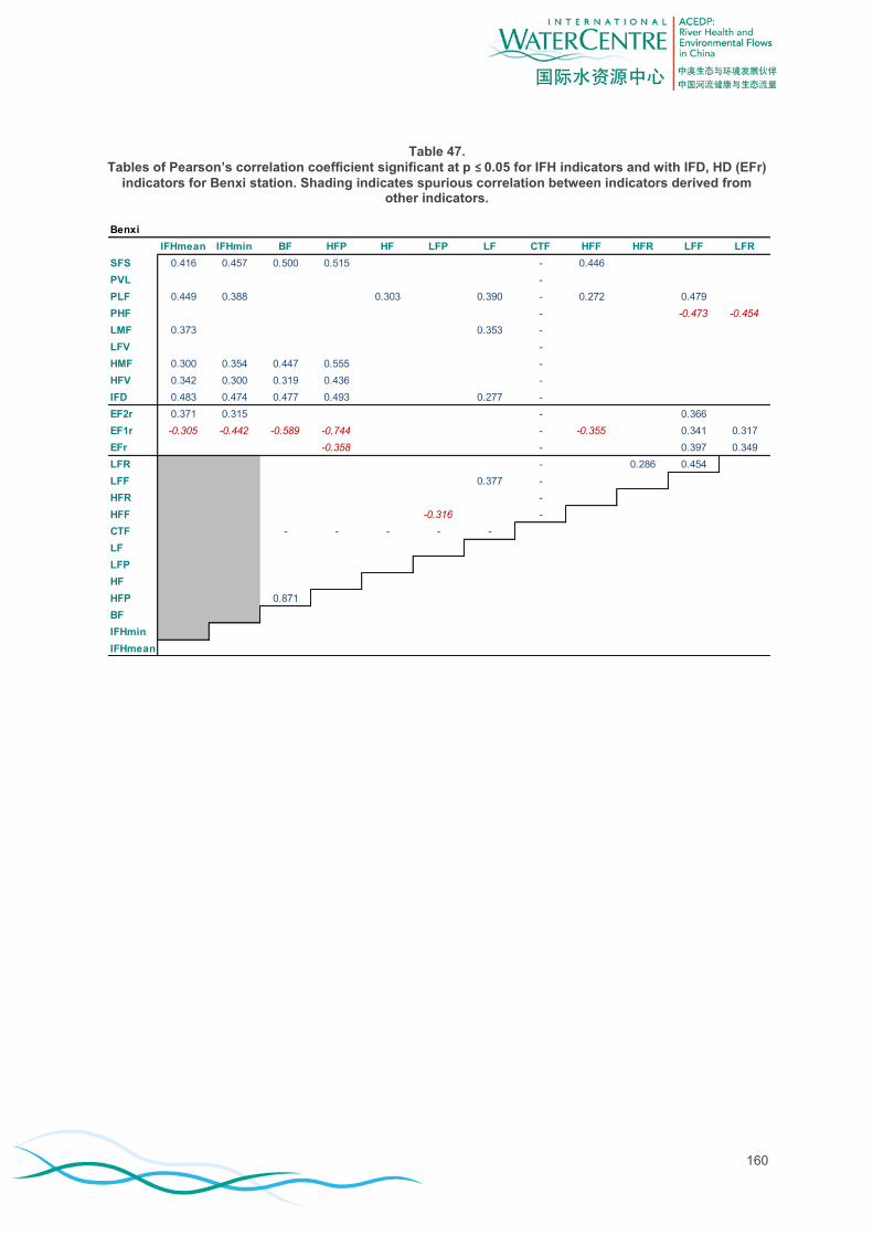
160

Table 47.

Tables of Pearson’s correlation coefficient significant at p ≤ 0.05 for IFH indicators and with IFD, HD (EFr)

indicators for Benxi station. Shading indicates spurious correlation between indicators derived from other indicators.

Benxi

IFHmean IFHmin BF HFP HF LFP LF CTF HFF HFR LFF LFR

SFS 0.416 0.457 0.500 0.515 - 0.446

PVL -

PLF 0.449 0.388 0.303 0.390 - 0.272 0.479

PHF - -0.473 -0.454

LMF 0.373 0.353 -

LFV -

HMF 0.300 0.354 0.447 0.555 -

HFV 0.342 0.300 0.319 0.436 -

IFD 0.483 0.474 0.477 0.493 0.277 -

EF2r 0.371 0.315 - 0.366

EF1r -0.305 -0.442 -0.589 -0.744 - -0.355 0.341 0.317

EFr -0.358 - 0.397 0.349

LFR - 0.286 0.454

LFF 0.377 -

HFR -

HFF -0.316 -

CTF - - - - -

LF

LFP

HF

HFP 0.871

BF

IFHmin

IFHmean

161

Table 48.


indicators for Liaoyang station. Shading indicates spurious correlation between indicators derived from other indicators.

Liaoyang

IFHmean IFHmin BF HFP HF LFP LF CTF HFF HFR LFF LFR

SFS 0.280 0.592 -0.361

PVL 0.575 0.559 0.542 0.333 0.425 0.710 0.436

PLF 0.605 0.510 0.537 0.389 0.450 0.546 0.483

PHF

LMF 0.552 0.578 0.450 0.327 0.473 0.716 0.435

LFV 0.356 0.315 0.332 0.302 0.384

HMF 0.341 0.362 0.300 0.327 0.428 0.292

HFV 0.510 0.430 0.428 0.392 0.620 0.502 0.273

IFD 0.666 0.663 0.588 0.486 0.722 0.576 0.566

EF2r 0.381 0.451 0.336 0.397 0.368

EF1r 0.494

EFr 0.414 0.488 0.333 0.414 0.388 0.370

LFR -0.418

LFF

HFR 0.563

HFF 0.313 0.347

CTF 0.731 0.609 0.672 0.574

LF 0.660 0.444 0.518

LFP -0.430

HF 0.653 0.519

HFP 0.655

BF

IFHmin

IFHmean

162

Table 49.


indicators for Xiaolinzi station. Shading indicates spurious correlation between indicators derived from other indicators.

Xiaolinzi

IFHmean IFHmin OB BF HFP HF LFP LF CTF HFF HFR LFF LFR

SFS 0.471 -

PVL 0.520 0.273 0.515 0.294 0.351 0.735 - 0.328

PLF 0.643 0.508 0.401 0.525 0.404 0.392 0.622 - 0.364

PHF -0.388 -0.571 -0.585 -

LMF 0.479 0.327 0.399 0.351 0.697 - 0.411

LFV 0.525 0.438 0.386 0.487 0.286 0.306 0.449 - 0.440

HMF 0.326 0.324 -

HFV 0.355 0.369 0.308 0.321 0.483 -

IFD 0.674 0.528 0.358 0.570 0.373 0.659 0.576 - 0.365

EF2r 0.543 0.451 0.343 0.376 0.392 0.378 - 0.311 0.371

EF1r 0.472 0.423 0.313 0.344 0.271 0.478 - 0.314

EFr 0.544 0.546 0.355 0.321 0.373 0.497 - 0.330 0.382

LFR - 0.493

LFF 0.318 -

HFR - 0.392

HFF 0.277 -

CTF - - - - - -

LF 0.631 0.285 0.490

LFP 0.352

HF 0.373 0.661

HFP 0.333 0.480

BF 0.496

OB

IFHmin

IFHmean

163

Table 50.


indicators for Tangmazhai station. Shading indicates spurious correlation between indicators derived from other indicators.

Relationship between IFH and IFD and HD indicators

Comparison of the overall index scores for IFH, IFD and HD (only EFr was available) for the Taizi River illustrates

a close relationship between IFH (mean) and IFD (Figure 103). The main difference in these two indicators is that

IFH (mean) has lower inter-annual variation. The lower inter-annual variability in IFH is explained by

consideration of the 5-year inter-annual frequency of event flow components in IFH, while IFD considers each

year independently. IFH (minimum) scores are considerably lower than IFH (mean), and the lowest score of any

indicator within the IFH suite might be too harsh for use as an overall score.

Compared to the IFH and IFD scores, the EFr score (based on daily flow data) was universally low in magnitude

(Figure 103). As previously discussed, this indicator is likely to score low for rivers in northern China regardless of

the degree of regulation. The EFr incorrectly indicated improved suitability of flows for the ecosystem at Benxi

after Guanyinge dam began operation in 1995 (Figure 103).

Discussion of IFH index The IFH index approach to assessment of stream hydrology for river health assessment has a number of

significant advantages over other simpler approaches, including:

Each of the indicators has an explicit link to ecosystem health, in particular those aspects related to the

key ecological assets.

The reference standards are not related to pristine hydrology, which in many places would be regarded

as unachievable, and perhaps not relevant. Rather, the hydrological standards are set according to the

desired state of ecological health, as determined using a scientific process.

The index is expressed in terms that relate directly to those aspects of the flow regime that are

manageable through implementation of an environmental flow regime. Thus, scores will reflect positive

management intervention.

Tangmazhai

IFHmean IFHmin OB BF HFP HF LFP LF CTF HFF HFR LFF LFR

SFS 0.394 0.300 - 0.557 0.294

PVL 0.328 0.352 - 0.320

PLF 0.421 0.461 0.451 0.561 -0.457 - 0.374

PHF -0.302 0.543 -

LMF -

LFV 0.396 -0.324 - 0.406

HMF 0.543 0.444 0.369 0.344 0.428 - 0.507

HFV 0.502 0.371 0.455 0.473 - 0.619 0.341

IFD 0.556 0.467 0.312 0.328 0.494 - 0.601 0.335

EF2r 0.374 0.471 0.448 0.297 0.459 -0.637 - 0.421

EF1r 0.321 -0.304 - 0.306

EFr 0.506 0.481 0.348 0.407 -0.417 - 0.360 0.350 0.352

LFR -0.319 - 0.464

LFF -0.352 -

HFR 0.293 - 0.607

HFF 0.402 0.540 -

CTF - - - - - -

LF

LFP

HF

HFP 0.427 0.590

BF

OB

IFHmin

IFHmean

164

Figure 103. Time series of overall IFH, IFD and EFr indicators for Taizi river stations. EFr scores calculated using daily flow data.

The main difficulty of deriving the IFH scores is not calculation of the scores per se, which requires only simple

algebra, but derivation of the environmental flow recommendations. Undertaking a holistic assessment of

0

10

20

30

40

50

60

70

80

90

100

0.0

0.1

0.2

0.3

0.4

0.5

0.6

0.7

0.8

0.9

1.0

EF

r In

dex s

co

re

IFH

an

d I

FD

In

dex s

co

re

Benxi

IFH mean

IFH min

IFD

EFr

0

10

20

30

40

50

60

70

80

90

100

0.0

0.1

0.2

0.3

0.4

0.5

0.6

0.7

0.8

0.9

1.0

EF

r In

dex s

co

re

IFH

an

d I

FD

In

dex s

co

re

Liaoyang

IFH mean

IFH min

IFD

EFr

0

10

20

30

40

50

60

70

80

90

100

0.0

0.1

0.2

0.3

0.4

0.5

0.6

0.7

0.8

0.9

1.0

EF

r In

dex s

co

re

IFH

an

d I

FD

In

dex s

co

re

Xiaolinzi

IFH mean

IFH min

IFD

EFr

0

10

20

30

40

50

60

70

80

90

100

0.0

0.1

0.2

0.3

0.4

0.5

0.6

0.7

0.8

0.9

1.0

EF

r In

dex s

co

re

IFH

an

d I

FD

In

dex s

co

re

Tangmazhai

IFH mean

IFH min

IFD

EFr

165

environmental flow needs is not a trivial exercise, so the application of IFH will be limited mostly to large river

mainstems, and rivers that are highly valued for their ecological and/or economic values.

Application of the IFH to the Taizi River demonstrated its power in rapidly and effectively highlighting those

components of the flow regime that were compromised by regulation. The IFD index scores were fairly closely

related to the IFH index scores, suggesting that the IFD could be a reasonable indicator for use in rivers where

an environmental flow assessment has not been undertaken.

Discussion and Conclusion

The IFH approach offers a fundamentally different way of assessing hydrology compared to that followed by the

FSR, HD and IFD approaches. The FSR, HD and IFD approaches attempt to answer for a test year, or test

period:

“Do general hydrological parameters, thought to be either universally important or universally

undesirable for maintaining good river health, have characteristics that are different to those of the

reference (natural or unimpaired) flow regime?”

The IFH approach attempts to answer the question for a test year, or test period:

“To what degree do specific hydrological parameters, identified as either locally important or locally

undesirable for maintaining river health to an agreed standard, occur in the current flow regime?”

The Flow Stress Ranking (FSR) indicators of hydrological alteration were calculated for the Taizi River mainstem,

a river that is heavily regulated by dams, and also for the Gui River mainstem and a tributary, the Goncheng

River, which are rivers that were not highly regulated over the test period. The FSR indicators are relatively easy

to calculate from monthly flows, and they show sensitivity to hydrological alteration. However, the results can be

difficult to interpret in terms of river health impacts, and do not necessarily assist in deciding the most appropriate

course of management action. The FSR indicators show impairment, whether the impact of regulation is to

increase the flow or reduce the flow, when reduced flow is usually the more serious concern from an ecological

perspective. Another problem is that the method ideally requires simulated reference and current flow series,

which are not generally available in China. If applied to a gauged flow series, the indicators only indicate the

broad impact of regulation on flows over a period of time. Without the availability of output from frequently

updated hydrological models, the method cannot realistically contribute to an annual river health report card. The

same limitation applies to most other indicators of hydrological alteration.

The HD index proposed for China’s nation-wide river health assessment program suffers some limitations in

terms of where it can be applied. In general, application of the HD method would be limited to rivers with

modelled reference flows, because these flows are required for calculation of the FD indicator. Where simulated

reference flows are available, the models are unlikely to be current in most places. The EF indicator is ideally

calculated from a daily flow series, which is not always readily available in China, further limiting the applicability

of the HD index. The FD indicator, which is based on the AAPFD index, was a good indicator of the volume of

water diverted from the river, but the conceptual link to ecosystem health was weak. The EF indicator is

grounded in the simple Tennant concept of relating hydrological factoring to ecosystem health. However, there

are doubts about the transferability of these factors to China. The EF indicator is also highly sensitive to natural

flow variability, such that: (i) the index score will typically show high inter-annual variability, and (ii) low to

moderate scores would be common, even in unregulated rivers, and especially in the drier rivers in the north of

China.

Given that in many places in China flow data is readily available only at the monthly time-step, and that there is a

need for a simple index of hydrological change that produces a score for each year, the Index of Flow Deviation

(IFD) was developed. The IFD measures flow alteration for each year based on comparison with pre-regulation

monthly flow data (or modelled reference flow data if available). The eight IFD indicators were selected to each

represent a particular aspect of the flow regime, the impairment of which was conceptually linked to ecosystem

health. The time series of IFD indicator scores represented a reasonable indicator of the pattern of change in flow

regime associated with regulation impacts, and also with periods that were naturally particularly wet or dry. The

166

selected indicators showed a degree of intercorrelation, but insufficient to warrant exclusion of any of the

indicators. The IFD index was also correlated with the HD index. The IFD index provides a reasonable

description of hydrological alteration, and can be applied in any river where pre-regulation flow data are available.

The calculated index scores cover a range of deviation from reference that would be expected to produce a

response in ecosystem health.




such flow recommendations should always be regarded as preliminary, and used only for planning purposes.

An Index of Flow Health (IFH) was developed and applied to the Taizi River main stem, using mean daily flow

series from 1953 to 2007. The method relies on undertaking an assessment of the environmental flow needs of

the river, and expressing the ecological needs in terms of well-specified flow components. These components

become the indicators of flow health. The IFH is measured as the degree of compliance of the flow components

with the standards expected for an agreed level of ecological stream health. A score can be calculated for each

year. The results can be presented as a time series of scores for each flow component, which identifies the most

impacted parts of the flow regime, and allows managers to evaluate the effectiveness of operational changes.

The stream health standards were determined within an environmental flows assessment framework using a mix

of expert opinion and flow-habitat and flow-geomorphology relationships from the literature. There are no suitable

ecological data available from the Taizi River to validate these standards for local conditions because: (i) the river

has been regulated for a long time, so recent ecological survey data reflect regulated conditions, and (ii) there are

a number of factors other than flow that compromise stream health, such as poor water quality, barriers, and

gravel extraction, so the influence of flow alteration on ecology is confounded.

The time series of IFH can be interpreted with respect to certain ecological data. Anadromous fish are vulnerable

to anthropogenic disturbance, such as habitat degradation from river engineering projects, water pollution and/or

overfishing (Li et al., 2007). One example of a species seriously impacted in this way in China is Coilia ectenes. It

was once a commercially important fishery resource in the middle and lower reaches of the Yangtze River and its

affiliated lakes. The anadromous stock is known to have declined dramatically since the late 1970s and 1980s,

especially after 1989 (Ma et al., 2010). For example, in the Yangtze estuary, the fish catch in 1973, a recorded

peak year, was 3.9 × 105 kg, but in 2003 the catch was only 2.5 × 10

4 kg (Li et al., 2007). Li et al. (2007) noted

that construction of the Three-Gorges Dam at the upper of the middle reach of the Yangtze River had the effect

of increasing the baseflow discharge from April until the flood season, which might increase energy expenditure

for migration and consequently further limit the migratory distance of C. ectenes. Similarly, in the Taizi River,

regulation by Tanghe and Shenwo dams from 1969, and then by Guanyinge from 1996, has reduced the

availability of flows suitable for successful completion of the spawning cycle of C. ectenes. Although this change

may have negatively impacted C. ectenes (which were not recorded in the 2009 survey), there are other factors

that may have been more important contributors to its decline, namely the construction of dikes that alienated

floodplain wetlands (potential spawning areas) from the channel, and poor water quality. In 2006, the National

Development and Reform Commission (2006) wrote that “At this time, the Liao is the most polluted river in China,

followed by the Hai He.” The 2008 State of the Environment Report indicated that the Taizi River below

Tangmazhai was worse than Grade V, and from Shenwo dam to Tangmazhai it was Grade V (Ministry of

Environmental Protection, 2009, p. 7).

The IFH requires more effort than simple computation of indicators from a hydrological data series (as for the HD

or IFD). Bio-assessment-based river health is normally measured at the local site-scale using field-based

sampling. At this scale, each river has peculiar hydraulic characteristics that are important to river biota,

processes and ecological health. Also, the relationships between a river’s geomorphological characteristics and

hydrological characteristics (which manifest as hydraulic characteristics) vary along its length. Thus, an effort is

required to understand the hydraulic and hydrological characteristics of the river under investigation, and also to

define river health in terms of the particular hydraulic and hydrological needs of the local ecological assets. This

is standard procedure for a holistic environmental flow assessment. A limitation is that under ideal conditions an

environmental flow assessment would involve a period of ecological monitoring, investigation of local flow-

ecology relationships, topographic-bathymetric field survey and hydraulic modelling – a process that requires

considerable time, funding and expertise.

167

In this report it was demonstrated how useful information can be derived on the hydraulics, hydrology,

geomorphology and ecology of a river system using existing data, general principles from the literature and

expert opinion. The environmental flow assessment component of the IFH calculation is not necessarily

undertaken with the expectation that river managers might apply the flow regime (although from the scientific

perspective, there is nothing preventing this). The main reason for undertaking the assessment is to set a

reference hydrological state specific to the ecological health requirements of the river under investigation. Once

this has been achieved, computation of the IFH index values to measure departure from the reference state is

straightforward. In rivers where a comprehensive environmental flow assessment has already been undertaken,

the IFH can simply be calculated from hydrological records.

As the IFH requires a greater effort than the simple IFD, a practical approach to national-scale assessment of

hydrological health could be to reserve the IFH for the main stems of major rivers, where resources are more

likely to be available to undertake environmental flow assessments, while the IFD could be applied elsewhere.

The two indicators were significantly correlated, which suggests that the IFD could be an ecologically relevant

indicator of hydrological alteration.

The annual hydrology index scores were related to annual discharge (Figure 104). This was expected, because

most hydrological statistics are related to annual discharge, and at the simplest level, annual discharge is an

indicator of hydrological stream health. As expected, both IFH and IFD scores were high in years with annual

discharge higher than the pre-dam median annual discharge (Figure 104). Index scores declined as the annual

discharge became lower, and generally low index scores should be expected for annual discharges lower than

50 percent of the pre-dam median annual discharge (Figure 104). This suggests the possibility of managing flows

to have a moderate or better hydrology index score in years with annual discharge higher than ~50 percent of the

pre-dam median, but to a large extent this depends on how the flows are distributed throughout the year.

Figure 104. Relationships between IFH and IFD indicators and annual discharge for Taizi river stations.

0.0

0.2

0.4

0.6

0.8

1.0

0% 50% 100% 150% 200% 250%

IFH

an

d I

FD

In

dex s

co

re

Percent of pre-dam median annual discharge

Benxi

IFH mean

IFD

0.0

0.2

0.4

0.6

0.8

1.0

0% 50% 100% 150% 200% 250%

IFH

an

d I

FD

In

dex s

co

re


Liaoyang

IFH mean

IFD

0.0

0.2

0.4

0.6

0.8

1.0

0% 50% 100% 150% 200% 250%

IFH

an

d I

FD

In

dex s

co

re


Xiaolinzi

IFH mean

IFD

0.0

0.2

0.4

0.6

0.8

1.0

0% 50% 100% 150% 200% 250%

IFH

an

d I

FD

In

dex s

co

re


Tangmazhai

IFH mean

IFD

168

The IFH is effective because it communicates to river managers those aspects of the flow regime needing

attention in order to improve river health. The environmental flow assessment documentation, compiled as part of

the IFH process, contains the necessary background and technical information on which river managers can

base their decisions to change flows for the benefit of river health. Of course, a process such as this relies on a

number of assumptions, and there will always be knowledge gaps that create uncertainty in the results. Ongoing

targeted research is the only way to address this issue. It may be that there are some general flow-ecology, flow-

geomorphology and flow-hydraulics relationships that can be widely applied, perhaps at the regional scale in

rivers of similar hydrologic and geomorphic character. Such relationships cannot be known until adequate

research effort has been expended on investigating them.

References

Andrews, E.D. 1983. Entrainment of gravel from naturally sorted riverbed material. Bulletin of the Geological

Society of America 94: 1225–1231.

Armitage, P.D. and Ladle, M. 1991. Habitat preferences of target species for application in PHABSIM testing. In

Bullock, A., Gustard, A. and Granger, E.S., Instream Flow Requirements of Aquatic Ecology in Two British Rivers,

Institute of Hydrology, Report No. 115, pp. 87-122. URL: http://nora.nerc.ac.uk/7351/1/IH_115.pdf (accessed 20

December 2010).

Arthington, A.H. and Long, G.C., Eds. 1997. Logan River trial of the Building Block Methodology for assessing

environmental flow requirements: background papers. Centre for Catchment and In-Stream Research and Dept

Natural Resources, Brisbane, Queensland.

Arthington, A.H. and Lloyd, R. Eds. 1998. Logan River trial of the Building Block Methodology for assessing

environmental flow requirements: workshop report. Centre for Catchment and In-Stream Research and Dept

Natural Resources, Brisbane, Queensland.

Arthington, A.H., Rall, J.L., Kennard, M.J. and Pusey, B.J. 2003. Environmental flow requirements of fish in

Lesotho rivers using the DRIFT methodology. River Research and Applications 19: 641-666.

Asaeda, T., Fujino, T. and Manatunge, J. 2005. Morphological adaptations of emergent plants to water flow: a

case study with Typha angustifolia, Zizania latifolia and Phragmites australis. Freshwater Biology 50(12): 1991-

2001.

Awaji, M. and Hanyu, I. 1987. Annual reproductive cycle of the wild type Medeka. Nippon Suisan Gakkaishi 53(6):

959-965. URL: http://rms1.agsearch.agropedia.affrc.go.jp/contents/JASI/pdf/society/35-1669.pdf (accessed 4

January 2011).

Baran, E. 2006. Fish migration triggers in the Lower Mekong Basin and other tropical freshwater systems. MRC

Technical Paper No. 14, Mekong River Commission, Vientiane, 56 pp. URL:

http://www.mrcmekong.org/download/free_download/Technical_paper14.pdf (accessed 17 November 2010)

Bartley, R. and Rutherfurd, I. 2005. Measuring the reach-scale geomorphic diversity of streams: application to a

stream disturbed by a sediment slug. River Research and Applications 21: 39–59.

Bartschi, D.K. 1976. A habitat-discharge method of determining instream flows for aquatic habitat. In Orsborn, J.F.

and Allman, C.H. (Eds), Proceedings of the Symposium and Speciality Conference on Instream Flow Needs II.

American Fisheries Society, Bethesda, Maryland. pp. 285–294.

Beard, L.R. 1974. Flood flow frequency techniques. Tech. Report CRWR119, Center for Research in Water

Resources, University of Texas at Austin, Austin, TX.

Bradford, M. J. 1997. An experimental study of stranding of juvenile salmonids on gravel bars and in side

channels during rapid flow decreases. Regulated Rivers: Research & Management, vol 13, 295-401.

http://nora.nerc.ac.uk/7351/1/IH_115.pdf

http://rms1.agsearch.agropedia.affrc.go.jp/contents/JASI/pdf/society/35-1669.pdf

http://www.mrcmekong.org/download/free_download/Technical_paper14.pdf

169

BPRWRP (Bureau of Pearl River Water Resources Protection) 2010. Background Report of Pear River

Demonstration Zone (Gui River Basin). Australia China Environment Development Partnership. River Health and

Environmental Flow, Guangzhou, April.

Brizga, S. 1998. Methods addressing flow requirements for geomorphological purposes. In Arthington, A.H. and

Zalucki, J.M. (eds) Comparative Evaluation of Environmental Flow Assessment Techniques: Review of Methods.

Occasional Paper No. 27/98. Land and Water Resources Research & Development Corporation, Canberra,

Australian Capital Territory, pp. 8–46. URL: http://lwa.gov.au/files/products/river-

landscapes/pr980309/pr980309.pdf (accessed 17 October 2010).

Brookes, A. 1995. The importance of high flows for riverine environments. In: Harper, D.M. and Ferguson, A.J.D.

(eds), The Ecological Basis for River Management. John Wiley & Sons, Chichester, pp. 33-49.

Buffington, J.M., and Montgomery, D.R. 1997. A systematic analysis of eight decades of incipient motion studies,

with special reference to gravel-bedded rivers. Water Resources Research 33: 1993–2029.

Bunn, S.E. and Arthington, A.H. 2002. Basic principles and ecological consequences of altered flow regimes for

aquatic biodiversity. Environmental Management 30: 492-507.

Caffrey, J., Barrett, P.R.F., Ferreira, M.T., Moreira, M.S., Murphy, K.J. and Wade, P.M. 1999. Biology, Ecology

and Management of Aquatic Plants. Proceedings of the 10th International Symposium on Aquatic Weeds,

European Weed Research Society. Kluwer Academic Publishers, Boston. Reprinted from Hydrobiologia 415, 339

pp.

Carling, P.A. 1983. Thresholds of coarse sediment transport in broad and narrow rivers. Earth Surface Processes

and Landforms 8: 1–18.

Carling, P.A. 1991. An appraisal of the velocity-reversal hypothesis for stable pool-riffle sequences in the River

Severn, England. Earth Processes and Landforms 16(1): 19-31.

Carpenter, S.R. and Lodge, D.M. 1986. Effects of submersed macrophytes on ecosystem processes. Aquatic

Botany 26: 341-370.

Chambers, P.A., Prepas, E.E., Hamilton, H.R. and Bothwell, M.L. Current velocity and its effect on aquatic

macrophytes in flowing waters. Ecological Applications 1: 249-257.

Chang, H.H. 1984. Formation of alternate bars. Journal of Hydraulic Engineering 111: 1412-1420.

Chang, H.H. 1988. Fluvial Processes in River Engineering, Krieger Publishing Company, Malabar, Florida, pp.

290-297.

Chee, Y.E., Webb, J.A., Stewardson, M. and Cottingham, P. 2009. Victorian environmental flows monitoring and

assessment program: Monitoring and evaluation of environmental flow releases in the Broken River. Report

prepared for the Goulburn Broken Catchment Management Authority and the Department of Sustainability and

Environment by eWater Cooperative Research Centre, Canberra. URL:

http://www.ewater.com.au/reports/ewater-crc-report_VEFMAP_Broken-River.pdf (accessed 4 January 2011).

Chessman, B.C., Fryirs, K.A., and Brierley, G.J. 2006. Linking geomorphic character, behaviour and condition to

fluvial biodiversity: implications for river management. Aquatic Conserv: Mar. Freshw. Ecosyst. 16: 267–288.

Chisholm, P.S., Ayers, H.D., Dickinson, W.T. and MacNab, I.D. 1976. Effects of altering streambed size on a

specific measure of biological diversity. Canadian Journal of Civil Engineering 3: 563–570.

Cottingham, P., Crook, D., Hillman, T., Roberts, J., Rutherfurd, I. and Stewardson, M. 2003. Environmental flow

recommendations for the Goulburn River below Lake Eildon. Unpublished report to the Department of

Sustainability and Environment, Victoria and the Murray Darling Basin Commission by CRC for Freshwater

Ecology and CRC for Catchment Hydrology. URL:

http://lwa.gov.au/files/products/river-landscapes/pr980309/pr980309.pdf

http://lwa.gov.au/files/products/river-landscapes/pr980309/pr980309.pdf

http://www.ewater.com.au/reports/ewater-crc-report_VEFMAP_Broken-River.pdf

170

http://www.ourwater.vic.gov.au/__data/assets/pdf_file/0006/28284/Goulburn-River.pdf (accessed 4 January

2011).

Cottingham, P., Stewardson, M. and Webb, A. 2005. Victorian Environmental Flows Monitoring and Assessment

Program: Stage 1 Statewide framework. CRC Freshwater Ecology and CRC Catchment Hydrology report to the

Department of Sustainability and Environment, Melbourne. URL:

http://freshwater.canberra.edu.au/Publications.nsf/3eb684c73f8449acca256f1200284afb/05bf3da07cb63473ca25

70bd00022c41/$FILE/VEFMAP%20Stage%201%20final%20report%20171105.pdf (accessed 4 January 2011).

CRAES 2010. Taizi Basin background report. Report to ACEDP project, International Water Centre, Brisbane.

Chinese Research Academy of Environmental Sciences, Ministry of Environmental Protection, Beijing.

Cushman, R.M. 1985. Review of ecological effects of rapidly varying flows downstream from hydroelectric

facilities. North American Journal of Fisheries Management 5: 330-339.

Davies, P., Harris, J., Hillman, T. and Walker, K. 2008. Sustainable Rivers Audit, SRA Report 1. A report on the

ecological health of rivers in the Murray-Darling Basin, 2004–2007. Prepared by the Independent Sustainable

Rivers Audit Group for the Murray–Darling Basin Ministerial Council, June. URL:

http://www2.mdbc.gov.au/SRA/river_health_check_-_sra_report_one.html (accessed 17 October 2010).

Davies, P.E., Harris, J.H., Hillman, T.J. and Walker, K.F. 2010. The Sustainable Rivers Audit: assessing river

ecosystem health in the Murray–Darling Basin, Australia. Marine and Freshwater Research 61(7): 764–777.

doi:10.1071/MF09043.

Doeg, T. 2004. Effect of Varying Environmental Objectives for Blackfish on Environmental Flow

Recommendations for Steels, Pauls and Dixons Creeks. Unpublished Report to the Steels, Pauls and Dixons

Creek Streamflow Management Plan Committee. URL:

http://www.melbournewater.com.au/content/library/rivers_and_creeks/stream_flow_management/stream_flow_re

ports/steels_creek_environmental_flow_study.pdf (accessed 4 January 2011).

Dollar, E.S.J. 2000. Fluvial geomorphology. Progress in Physical Geography 24(3): 385-406.

Downes, B.J., Lake, P.S., Schreiber, E.S.G. and Glaister, A. 1998. Habitat structure and regulation of local

species diversity in a stony upland stream. Ecological Monographs 68: 237–257.

Duan, Q.Y., Sorooshian, S. and Gupta, V. 1992. Effective and Efficient Global Optimization for Conceptual

Rainfall-Runoff Models. Water Resources Research 28(4): 1015-1031.

Dungsheng, L. 1985. Loess and Environment. Science Press, Beijing (in Chinese).

eChinacities 2010. Guilin, Lijiang River tour to shorten boat route due to ongoing drought. Mar 24, 2010

eChinacities.com. URL: http://www.echinacities.com/guilin/city-in-pulse/guilin-lijiang-river-tour-to-shorten-boat-

route-due-to.html (accessed 31 May 2011).

Egiazaroff, I.V. 1965. Calculation of non-uniform sediment concentrations. Journal of Hydraulic Engineering,

Proceedings of the American Society of Civil Engineers 91(HY4): 225-248.

Feng, X.Q., Zhang, G.X. and Yin, X.R. 2010a. Calculation of ecological water requirements in the lower reaches

of the Taizi River based on ecological protection objectives. J. Acta Scientiae Circumstantiae 30(7): 1466-1471.

Feng, X.Q., Zhang, G.X. and Yin, X.R. 2010b. Calculation of instream ecological water requirement of Taizi River

based on the allocation of ecological water right. Chinese Journal of Ecology 29(7): 1398-1402.

Florsheim, J.L., Mount, J.F. and Chin, A. 2008. Bank erosion as a desirable attribute of rivers. BioScience 58(6):

519-529.

Franklin, P., Dunbar, M. and Whitehead, P. 2008. Flow controls on lowland river macrophytes: A review. Science

of the Total Environment 400: 369-378.

http://www.ourwater.vic.gov.au/__data/assets/pdf_file/0006/28284/Goulburn-River.pdf

http://freshwater.canberra.edu.au/Publications.nsf/3eb684c73f8449acca256f1200284afb/05bf3da07cb63473ca2570bd00022c41/$FILE/VEFMAP%20Stage%201%20final%20report%20171105.pdf

http://freshwater.canberra.edu.au/Publications.nsf/3eb684c73f8449acca256f1200284afb/05bf3da07cb63473ca2570bd00022c41/$FILE/VEFMAP%20Stage%201%20final%20report%20171105.pdf

http://www2.mdbc.gov.au/SRA/river_health_check_-_sra_report_one.html

http://www.melbournewater.com.au/content/library/rivers_and_creeks/stream_flow_management/stream_flow_reports/steels_creek_environmental_flow_study.pdf

http://www.melbournewater.com.au/content/library/rivers_and_creeks/stream_flow_management/stream_flow_reports/steels_creek_environmental_flow_study.pdf

http://www.echinacities.com/guilin/city-in-pulse/guilin-lijiang-river-tour-to-shorten-boat-route-due-to.html

http://www.echinacities.com/guilin/city-in-pulse/guilin-lijiang-river-tour-to-shorten-boat-route-due-to.html

171

Frings, R.M. 2008. Downstream fining in large sand-bed rivers. Earth-Science Reviews 87: 39-60.

Fu, G. Chen, S., Liu, C. and Shepard, D. 2004. Hydro-climatic trends of the Yellow River basin for the last 50

years. Climatic Change 65: 149-178.

Fujuro, Y. and Tomiyama, K. 2000. Distribution and microhabitat of coexisting two freshwater snail species,

Semisulcospira libertina (Gould)(Prosobranchia; Pleuroceridae) and Clithon retropictus (Martens)(Prosobranchia :

Neritidae). The Japanese journal of malacologym Venus 59(3): 245-260.

Gehrke, P.C., Brown, P., Schiller, C.B., Moffatt, D.B. and Bruce, A.M. 1995. River regulation and fish

communities in the Murray-Darling System, Australia. Regulated Rivers: Research and Management 11: 363-375.

Gilroy, D.J., Jensen, P., Allen, B.C., Chandra, S., Ganzorig, B., Hogan, Z., Maxted, J.T. and Vander Zanden, M.J.

2010. Home range and seasonal movement of taimen, Hucho taimen, in Mongolia. Ecology of Freshwater Fish

19(4): 545-554.

Gippel, C.J. 1995. Environmental hydraulics of large woody debris in streams and rivers. Journal of

Environmental Engineering 121: 388-395.

Gippel, C.J. 2001a. Hydrological analyses for environmental flow assessment. In Proceedings MODSIM 2001,

International Congress on Modelling and Simulation, Modelling & Simulation Society of Australia & New Zealand,

Ghassemi, F. and Whetton, P. (Eds), The Australian National University, Canberra, pp. 873-880. URL:

http://www.mssanz.org.au/MODSIM01/Vol%202/Gippel.pdf (accessed 17 October 2010).

Gippel, C.J. 2001b. Geomorphic issues associated with environmental flow assessment in alluvial non-tidal rivers.

Australian Journal of Water Resources 5(1):3-19.

Gippel, C.J. 2002. The Victorian Snowy River: Review of Historical Environmental Change and Proposed

Rehabilitation Options. Report by Fluvial Systems Pty Ltd, Melbourne in association with EarthTech Pty Ltd, to

East Gippsland Catchment Management Authority, Bairnsdale, Vic.

Gippel, C.J. and Speed, R. 2010. Environmental Flow Assessment Framework and Methods, Including

Environmental Asset Identification and Water Re-allocation. ACEDP Australia-China Environment Development

Partnership, River Health and Environmental Flow in China. International Water Centre Pty Ltd, Brisbane,

February.

Gippel, C.J., Marsh, N. and Grice, T. 2012a. Flow Health - Software to assess the deviation of river flows from

reference and to design a monthly environmental flow regime. Technical Manual and User Guide, Version 1.0.

ACEDP Australia-China Environment Development Partnership, River Health and Environmental Flow in China.

International WaterCentre, Brisbane, Fluvial Systems Pty Ltd, Stockton, and Yorb Pty Ltd, Brisbane, January.

Gippel, C.J., Jiang, X., Fu, X., Liu, X., Chen, L., Wang, H.Z., Jin, S., Li, L., Wang, L., Sun, Y. Pang, H., Song, R.,

Sun, F., Shang, H. and Speed, R. 2012b. Assessment of river health in the lower Yellow River. ACEDP Australia-

China Environment Development Partnership, River Health and Environmental Flow in China. Yellow River

Conservancy Commission, Ministry of Water Resources and the International WaterCentre, Brisbane, April.

Gippel, C.J., Bond, N.R., James, C. and Wang, X. 2009a. An asset-based, holistic, environmental flows

assessment approach. Water Resources Development 25(2): 305-333.

Gippel, C.J., Cosier, M., Markar, S. and Liu, C. 2009b. Balancing environmental flow needs and water supply

reliability. Water Resources Development 25(2): 335-357.

Gordon, N.D. 1995. Summary of technical testimony in the Colorado Water Division 1 Trial. Engineers Inc. US

Forest Service, Fort Collins, CO, September.

Gordon, N.D., McMahon, T.A., Finlayson, B.L., Gippel, C.J. and Nathan, R.J. 2004. Stream Hydrology: An

Introduction for Ecologists. Second Edition, John Wiley & Sons, Chichester.

Gorman, O.T. and Karr, J.R. 1978. Habitat structure and stream fish communities. Ecology 59: 507–515.

http://www.mssanz.org.au/MODSIM01/Vol%202/Gippel.pdf

172

Grayson, R.B., Argent, R.M., Nathan, R.J., McMahon, T.A. and Mein, R. 1996. Hydrological Recipes: Estimation

Techniques in Australian Hydrology. Cooperative Research Centre for Catchment Hydrology, Australia, 125 pp.

Groeneveld, D.P. and French, R.H. 1995. Hydrodynamic control of an emergent aquatic plant (Scirpus acutus) in

open channels. Water Resources Bulletin 31: 505-514.

Growns, J. and Marsh, N. 2000. Characterisation of flow in regulated and unregulated streams in eastern

Australia. Cooperative Research Centre for Freshwater Ecology Technical Report 3/2000. Cooperative Research

Centre for Freshwater Ecology and Centre for Environmental Applied Hydrology. University of Canberra,

Canberra. September. URL:

http://freshwater.canberra.edu.au/Publications.nsf/0/7210558ce2ac5b31ca256f0b0022e017/$FILE/Flows.pdf

(accessed 17 November 2010).

Guscio, F.J., Bartley, T.R. and Beck, A.N. 1965. Water resources problems generated by obnoxious plants.

Proceedings of the American Society of Civil Engineers, Journal of the Waterways and Harbours Division 10: 47-

60.

Hancock, P.J. and Boulton, A.J. 2005. The effects of an environmental flow release on water quality in the

hyporheic zone of the Hunter River, Australia. Hydrobiologia 552: 75-85.

Hey, R.D., Thorne C.R. and Newson, M.D. 1997. Applied Fluvial Geomorphology for River Engineers and

Management. Wiley, Chichester.

Hicks, D.M. and Mason, P.D. 1991. Roughness Characteristics of New Zealand Rivers. Water Resources Survey,

Department of Scientific and Industrial Research, Marine and Freshwater, Wellington, New Zealand.

Hill, M.T., Platts, W.S. and Beschta, R.L. 1991. Ecological and geomorphological concepts for instream and out-

of-channel flow requirements. Rivers 2(3): 198–210.

Hupp, C.R. and Osterkamp, W.R. 1996. Riparian vegetation and fluvial geomorphic processes. Geomorphology,

14: 277-295.

Ikeda, S. 1983. Flow and bed topography in channels with alternate bars. In Elliot, C.M. (Ed.) River Meandering,

Proceedings of the Conference Rivers ’83. Waterway, Port, Coastal and Ocean Division of the American Society

of Civil Engineers, New Orleans, Louisiana, pp. 733-746.

Ikeda, S. 1984. Prediction of alternate bar wavelength and height. Journal of Hydraulic Engineering 100: 371-386.

IRTCES 2004. Sediment issues of the Haihe and Lioahe Rivers in China. Contract No. 861.368.4. International

Research and Training Center on Erosion and Sedimentation. Beijing, December. URL:

www.irtces.org/isi/isi_document/861-368-4-english.pdf (accessed 17 October 2010).

Jaeggi, M. 1984. Formation and effects of alternate bars. Journal of Hydraulic Engineering, ASCE 110: 142-156.

Jiang, X., Arthington, A. and Liu, C. 2010. Environmental flow requirements of fish in the lower reach of the

Yellow River. Water International 35 (4): 381–396.

JICA 2000. Guanyinge Multipurpose Dam Project. Japan International Cooperation Agency, Tokyo. URL:

http://www.jica.go.jp/english/operations/evaluation/oda_loan/post/2000/pdf/02-01.pdf (accessed 17 October

2010).

Jowett, I.G. and Duncan, M.J. 1990. Flow variability in New Zealand rivers and its relationship to in-stream

habitat and biota, N.Z. J. Marine and Freshwater Res. 24: 305-317.

Julien, P.Y. 1995. Erosion and Sedimentation. Cambridge University Press, Cambridge.

Keller, E.A. 1972. Development of alluvial stream channels, a five stage model. Geological Society of America

Bulletin 83: 1531-1540.

http://freshwater.canberra.edu.au/Publications.nsf/0/7210558ce2ac5b31ca256f0b0022e017/$FILE/Flows.pdf

http://www.irtces.org/isi/isi_document/861-368-4-english.pdf

http://www.jica.go.jp/english/operations/evaluation/oda_loan/post/2000/pdf/02-01.pdf

173

Kemp, J., Harper, D.M. and Crosa, G.A. 1999. Use of ‘functional habitats’ to link ecology with morphology and

hydrology in river rehabilitation. Aquatic Conservation: Marine and Freshwater Ecosystems 9: 159-178.

Kennard, M.J., Mackay, S.J., Pusey, B.J., Olden, J.D. and Marsh, N. 2010. Quantifying uncertainty in estimation

of hydrologic metrics for ecohydrological studies. River Research and Applications 26(2): 137-156.

King, J., Brown, C. and Sabet, H. 2003. A scenario-based holistic approach to environmental flow assessments

for river. River Research and Applications 19: 619-639.

King, J.M., Tharme, R.E. and Brown, C.A. 1999. Definition and Implementation of Instream Flows. Thematic

Report for the World Commission on Dams. Southern Waters Ecological Research and Consulting, Cape Town.

Kitamura, W. and Kobayashi, M. 2003. The effect of water flow on spawning in the medaka, Oryzias latipes. Fish

Physiology and Biochemistry 28(1-4): 429-430.

Koger, C.S., Teh, S.J. and Hinton, D.E. 1999. Variations of light and temperature regimes and resulting effects on

reproductive parameters in Medaka (Oryzias latipes). Biology of Reproduction 61(5): 1287-1293.

Kolasa, J. and Rollo, D. 1991. Introduction: the heterogeneity of heterogeneity: a glossary. In Kolasa, J., Pickett,

S.T.A. (eds), Ecological Heterogeneity. Springer-Verlag, New York, pp. 1–24.

Komar, P.D. 1987. Selective gravel entrainment and the empirical evaluation of flow competence. Sedimentology

34:1165–1176.

Kotusz, J., Krappe, M., Kusznierz, J., Propiolek, M., Riel, P., Waterstraat, A. and Witkowski, A. 2004. Distribution,

density and habitat of Cottus poecilopus (Heckel, 1836) in Lake Hancza (North East Poland) as compared with

the situation in the Luzin lakes (North East Germany). Verhandlungen der Gesellschaft für Ichthyologie Band 4:

91-105. URL: http://www.gnl-kratzeburg.de/staff/waterstraat/pub/Kotusz_et_al_75dpi.pdf (accessed 4 January

2011).

Kuczera, G. and Franks, S. 2006. Book IV – Estimation of peak discharges. Draft for review. Australian Rainfall &

Runoff – a Guide to Flow Estimation (4th Edition). National Committee on Water Engineering, Institution of

Engineers, Australia, Barton, ACT. URL: http://www.ncwe.org.au/arr/detail_toc.html (accessed 17 December

2010).

Kumiko, S. and Misako, U. 2004. Drift and Upstream Movement of Semisulcospira libertina (Caenogastropoda:

Pleuroceridae) in a Natural Stream. The Japanese journal of malacology, Venus 63(1/2): 49-59.

Ladson, A.R. and White, L.J. (1999) An Index of Stream Condition: Reference Manual. Prepared for Waterways

Unit, Department of Natural Resources and Environment, 2nd Ed. Melbourne, Vic.

Ladson, A.R., White, L.J., Doolan, J.A., Finlayson, B.L., Hart, B.T., Lake, P.S. and Tilleard, J.W. 1999.

Development and testing of an Index of Stream Condition for waterway management in Australia. Freshwater

Biology 41: 453-468.

Lake, P.S. 2000. Disturbance, patchiness, and diversity in streams. Journal of the North American Benthological

Society 19: 573–592.

Lancaster, J., Downes, B.J. and Reich, P. 2003. Linking landscape patterns of resource distribution with models

of aggregation in ovipositing stream insects. Journal of Animal Ecology 72: 969–978.

Lancaster, J. and Downes, B.J. 2010. Linking the hydraulic world of individual organisms to ecological processes:

putting ecology into ecohydraulics. River Research and Applications 26: 385-403.

Leslie, D.J. 2001. Effect of river management on colonially-nesting waterbirds in the Barmah-Millewa Forest,

South-Eastern Australia. Regulated Rivers: Research & Management 17: 21-36.

Leslie, D.J. and Ward, K.A. 2002. Murray River environmental flows 2000-2001. Ecological Management &

Restoration 3(3): 221-223.

http://www.gnl-kratzeburg.de/staff/waterstraat/pub/Kotusz_et_al_75dpi.pdf

174

Lester, R.E. and Boulton, A.J. 2008. Rehabilitating agricultural streams in Australia with wood: a review.

Environmental Management 42: 310-326.

Li, S and Xu, S. 1995. Culture and Capture of Fish in Chinese Reservoirs. Southbound, International

Development Research Centre, 140 p.

Li, W. and Xu, S. 2006. Study of water required for ecological environment in Taizi River. Journal of Dalian

University of Technology 46(1): 116-120. (In Chinese with English summary).

Li, Y., Xie, S., Li, Z., Gong, W. and He, W. 2007. Gonad development of an anadromous fish Coilia ectenes

(Engraulidae) in lower reach of Yangtze River, China. Fisheries Science 73: 1224-1230.

Loddon River Environmental Flows Scientific Panel, 2002. Environmental Flow Determination of the Loddon

River Catchment: Final Report. Unpublished Report to the North Central Catchment Management Authority and

Department of Natural Resources and Environment, Melbourne, Victoria. URL:

http://www.ourwater.vic.gov.au/__data/assets/pdf_file/0011/28298/Loddon-River.pdf (accessed 4 January 2011).

Lorang, M.S. and Hauer, F.R. 2003. Flow competence and streambed stability: an evaluation of technique and

application. Journal of the North American Benthological Society 22(4):475–491.

LUCRPO, LPSRIEP and Montgomery Watson 2001. Environmental Impact Assessment report for the Liao River

Basin Project. Liaoning Urban Construction and Renewal Project Office, Liaoning Provincial Scientific Researrch

Institute for Environmental Projection and Montgomery Watson. E430, Vol 1. URL:

http://info.worldbank.org/etools/docs/library/39794/Sample-EAreportLiaoRiverBasinProjectEN.pdf (accessed 17

November 2010).

Lyne, V. and Hollick, M. 1979. Stochastic time-variable rainfall-runoff modeling. In Hydrology and Water

Resources Symposium, Perth. Institution of Engineers Australia National Conference Publication 79/10,

Institution of Engineers Australia, Canberra, ACT, pp. 89–93.

Ma, C., Cheng, Q., Zhang, Q., Zhuang, P. and Zhao, Y. 2010. Genetic variation of Coilia ectenes (Clupeiformes:

Engraulidae) revealed by the complete cytochrome b sequences of mitochondrial DNA. Journal of Experimental

Marine Biology and Ecology 385: 14–19.

Ma, C., Liu, M., Ma, L., Zhang, F. and Chen Y. 2004. Genetic diversity in Coilia ectenes by RAPD analysis.

Marine Fisheries Research 25: 19–24 (in Chinese with English abstract).

Mackay, S. and Marsh, N. 2005. The response of aquatic macrophytes to riparian shading in a stream

rehabilitation site. Cooperative Research Centre for Catchment Hydrology, Technical Report 05/5, April. URL:

http://www.catchment.crc.org.au/pdfs/technical200505.pdf (accessed 17 October 2010).

Madsen, J.D., Chambers, P.A., James, W.F., Koch, E.W. and Westlake, D.F. 2001. The interaction between

water movement, sediment dynamics and submersed macrophytes. Hydrobiologia 444: 71-84.

Mann, J.L. 2006. Instream flow methodologies: an evaluation of the Tennant Method for higher gradient streams

in the National Forest System lands in the western U.S. Master of Science Thesis. Colorado State University,

Fort Collins CO.

Mathews, R.C. Jr and Bao, Y. 1991. The Texas Method of preliminary instream flow assessment. Rivers

2(4):295-310.

McBain, S. and Trush, B. 1997. Thresholds for managing regulated river ecosystems. In Sommarstrom, S. (ed.),

Proc sixth biennial watershed management conference, 23-25 October 1996, Lake Tahoe, CA/NV. Centers for

Water and Wildland resources, Water Resources Center Report No. 92, University of California, Davis, April, pp.

11-13.

http://www.ourwater.vic.gov.au/__data/assets/pdf_file/0011/28298/Loddon-River.pdf

http://info.worldbank.org/etools/docs/library/39794/Sample-EAreportLiaoRiverBasinProjectEN.pdf

http://www.catchment.crc.org.au/pdfs/technical200505.pdf

175

McCoy, E.D. and Bell, S.S. 1991. Habitat structure: the evolution and diversification of a complex topic. In Habitat

Structure—the Physical Arrangement of Objects in Space. In Bell, S.S., McCoy, E.D. and Mushinsky H.R. (eds).

Chapman and Hall, London, pp. 3–21.

Miao, C., Ni, J. and Borthwick, A. 2010. Recent changes of water discharge and sediment load in the Yellow

River basin, China. Progress in Physical Geography 34(4): 541–561.

MDBC 2003. Hydrology Theme, Summary of Pilot Audit Technical Report – Sustainable Rivers Audit. MDBC

Publication 08/04. Murray-Darling Basin Commission, Canberra, ACT.

Ministry of Environmental Protection 2009. Report on the State of the Environment in China, 2008. Ministry of

Environmental Protection of the People’s Republic of China. URL:

http://english.mep.gov.cn/standards_reports/soe/soe2008/201002/t20100224_186081.htm (accessed 4 January

2011).

Moggridge, H.L. and Gurnell, A.M. 2010. Hydrological controls on the transport and deposition of plant

propagules within riparian areas. River Research and Applications 26: 512-527.

Montgomery, D.R., Collins, B.D., Buffington, J.M. and Abbe, T.B. 2003. Geomorphic effects of wood in rivers. In:

Gregory, S.V., Boyer, K.L., Gurnell, A.M. (eds), The ecology and management of wood in world rivers. American

Fisheries Society Symposium 37: 21-47. URL: http://riverhistory.ess.washington.edu/pubs/WoodinRivers.pdf

(accessed 17 October 2010).

MTP (Mongolian Taimen Project) 2008. Taimen (Hucho taimen). URL:

http://limnology.wisc.edu/mongolia/Taimen.htm (accessed 4 January 2011).

Nathan, R.J. and McMahon, T.A. 1990. Evaluation of automated techniques for baseflow and recession analysis.

Water Resources Research 26: 1465-1473.

National Development and Reform Commission 2006. Rivers and Lakes Identified for Environmental Protection.

Cleaner Production in China. NDRC. URL: http://www.chinacp.org.cn/eng/cppolicystrategy/cp_rivers_lakes.html

(accessed 4 January 2011).

Norris, R.H. and Thoms, M.C. 1999. What is river health? Freshwater Biology 41: 97–209.

NRM South 2009. Hydrology User’s Guide. Tasmanian River Condition Index, Book 2. NRM South, South Hobart.

URL: http://www.nrmsouth.org.au/uploaded/287/15130399_02trcihydrologyfieldmanua.pdf (accessed 17 October

2010).

NTWGHARL 2010. Indicators, standards and methods for river health assessment. Technical document for the

health assessment of national-wide rivers and lakes, for pilot work, Version 1.0. National Technical Working

Group for the Health Assessment of Rivers and Lakes, Department of Water Resources Management, Ministry of

Water Resources People’s Republic of China, Beijing.

Old, G. and Acreman, M. 2006. Guidance on compensation flows and freshets Task 3 Literature review.

SNIFFER Project WFD82. Centre for Ecology & Hydrology, Wallingford, OX. Scotland and Northern Ireland

Forum for Environmental Research, Edinburgh. URL:

http://www.wfduk.org/LibraryPublicDocs/WFD82_Task_2_report_guidance_freshwater (accessed 17 December

2010).

Olsen, D.S., Whitaker, A.C. and Potts, D.F. 1997. Assessing stream channel stability thresholds using flow

competence estimates at bankfull stage. Journal of the American Water Resources Association 33: 1197–207.

Petts, G.E. 1979. Complex response of river channel morphology subsequent to reservoir construction. Progress

in Physical Geography 3: 329– 362.

Petts, G.E. and Gurnell, A.M. 2005. Dams and geomorphology: Research progress and future directions.

Geomorphology 71: 27-47.

http://english.mep.gov.cn/standards_reports/soe/soe2008/201002/t20100224_186081.htm

http://riverhistory.ess.washington.edu/pubs/WoodinRivers.pdf

http://limnology.wisc.edu/mongolia/Taimen.htm

http://www.chinacp.org.cn/eng/cppolicystrategy/cp_rivers_lakes.html

http://www.nrmsouth.org.au/uploaded/287/15130399_02trcihydrologyfieldmanua.pdf

http://www.wfduk.org/LibraryPublicDocs/WFD82_Task_2_report_guidance_freshwater

176

Pickup, G. and Marks, A. 2001. Identification of floodplains and estimation of floodplain flow velocities for

sediment transport modelling. CSIRO Land & Water, Technical Report 10/01, July 2001, pp. 26. URL:

http://www.clw.csiro.au/publications/technical2001/tr14-01.pdf (accessed 17 November 2010).

Poff, N.L. 1997. Landscape filters and species traits: towards mechanistic understanding and prediction in stream

ecology. Journal of the North American Benthological Society 16: 391–409.

Poff, N.L., Allan, J.D., Bain, M.B., Karr, J.R., Prestegaard, K.L., Richter, B.D., Sparks, R.E. and Stromberg, J.C.

1997. The natural flow regime, a paradigm for river conservation and restoration. BioScience 47: 769-784.

Poff, N.L., Richter, B., Arthington, A.H., Bunn, S.E., Naiman, R.J. Kendy, E., Acreman, M., Apse, C., Bledsoe,

B.P., Freeman, M., Henriksen, J., Jacobson, R.B., Kennen, J., Merritt, D., O’Keefe, J., Olden, J.D., Rogers, K.,

Tharme, R. and Warner, A.T. 2009. The ecological limits of hydrologic alteration (ELOHA): a new framework for

developing regional environmental flow standards. Freshwater Biology 55(1): 147-170.

Potter, D.J. and Pilgrim, D.H. 1971. Flood estimation using a regional flood frequency approach. Final Report, Vol

2: Report on Analysis Components. Australian Water Resources Council, Research Project 68/1, Hydrology of

Small Rural Catchments. Snowy Mountains Engineering Corporation, Cooma.

Powell, M.D. 2009. Dryland rivers: processes and forms. In Parsons, A.J. and Abrahams, A.D. (eds),

Geomorphology of Desert Environments, 2nd

ed., Springer, pp. 333-373.

Reiser, D.W., Ramey, M.P. and Lambert, T.R. 1985. Review of flushing flow requirements in regulated streams.

Pacific Gas and Electric Co. Department of Engineering Research. San Remon, CA.

Resh, V.H., Brown, A.V., Covich, A.P., Gurtz, M.E., Li, H.W., Minshall, G.W., Reice, S.R., Sheldon, A.L., Wallace,

J.B. and Wissmar, R. 1988. The role of disturbance in stream ecology. Journal of the North American

Benthological Society 7: 433–455.

Richards, K.S. 1982 Rivers, form and process in alluvial channels, Methuen, New York.

Richards, K.S., Brasington, J. and Hughes, F. 2002. Geomorphic dynamics of floodplains: ecological implications

and a potential modelling strategy. Freshwater Biology 47: 559-579.

Richter, B.D, Baumgartner, J.V., Powell, J. and Braun, D.P. 1996. A method for assessing hydrologic alteration

within ecosystems. Conservation Biology 10: 1163–1174.

Richter, B.D., Baumgartner, J.V., Wigington, R. and Braun, D.P. 1997. How much water does a river need?

Freshwater Biology 37: 231-249.

Riis, T. and Biggs, B.J.F. Hydrologic and hydraulic control of macrophyte establishment and performance in

streams. Limnology and Oceanography 48: 1488-1497.

Riis, T., Suren, A.M., Clausen, B. and Sand-Jensen, K. 2008. Vegetation and flow regime in lowland streams.

Freshwater Biology 53: 1531-1543.

Riley, S.J. 1972. A comparison of morphometric measures of bankfull. Journal of Hydrology 17: 23-31.

Rowntree, K.M. and Wadeson, R.A. 1997. A hierarchical model for the assessment of instream flow requirements.

Geoöko plus 4: 85–100.

Saltveit, S.J., Halleraker, J.H., Arnekleiv, J.V and Harby, A. 2001. Field experiments on stranding in juvenile

Atlantic salmon (salmo salar) and brown trout (salmo trutta) during rapid flow decreases caused by hydropeaking.

Journal of Regulated Rivers 17: 609-622.

Schmidt, L.J. and Potyondy, J.P. 2004. Quantifying channel maintenance instream flows: an approach for gravel-

bed streams in the Western United States. Gen. Tech. Rep. RMRS-GTR-128. U.S. Department of Agriculture,

Forest Service, Rocky Mountain Research Station, Fort Collins, CO, 33 p. URL:

www.stream.fs.fed.us/news/streamnt/pdf/jul04.pdf (accessed 17 October 2010).

http://www.clw.csiro.au/publications/technical2001/tr14-01.pdf

http://www.stream.fs.fed.us/news/streamnt/pdf/jul04.pdf

177

Shields, A. 1936. Anwendung der Aehnlichkeitsmechanik und der Turbulenzforschung auf die

Geschiebebewegung. Mitteilungen der Preuiβischen ersuchsanstalt fur Wasserbau und Schiffbau, 26, 26 p.

Shireman, J.V. and Smith, C.R. 1983. Synopsis of biological data on the grass carp. FAO Fisheries Synopsis 135,

Rome, 86 pp.

SKM, CRC for Freshwater Ecology, Freshwater Ecology (NRE) and Lloyd Environmental Consultants 2002. The

FLOWS Method – a method for determining environmental water requirements in Victoria. Report prepared by

Sinclair Knight Merz, the Cooperative Research Centre for Freshwater Ecology, Freshwater Ecology (NRE) and

Lloyd Environmental Consultants. Department of Natural Resources and Environment, Melbourne. URL:

http://www.envict.org.au/file/Flows_Methodology.pdf (accessed 17 October 2010).

SKM (Sinclair Knight Merz) 2005. Development of a Flow Stressed Ranking Procedure. Final Report to

Department of Sustainability and Environment, Victoria. Sinclair Knight Merz, Armadale, Victoria.

Su, F., Chen, M., Dong, Z. and Xu, Z. 2006. Minimum ecological discharge of Liaohe River. Journal of Hohai

University (Natural Sciences) 34(2): 136-139. (In Chinese with English abstract).

Suen, J.P. and Herricks, E.E. 2009. Developing fish community based ecohydrological indicators for water

resources management in Taiwan. Hydrobiologia 625: 223-234.

Tennant, D.L. 1976. Instream flow regimens for fish, wildlife, recreation and related environmental resources.

Fisheries 1(4): pp. 6-10.

Texas Parks and Wildlife Department 2003. Environmental Flow Targets: Planning Criteria of the Consensus

State Water Plan. Austin.

Tharme, R.E. 2003. A global perspective on environmental flow assessment: emerging trends in the development

and application of environmental flow methodologies for rivers. River Research and Applications 19(5-6): 397-

441.

Tharme, R.E. and King, J.M. 1998. Development of the Building Block Methodology for instream flow

assessments and supporting research on the effects of different magnitude flows on riverine ecosystems. WRC

Report no. 576/1/98. Freshwater Research Unit, University of Capetown, Capetown.

Townsend, C.R. 1989. The patch dynamics concept of stream community structure. Journal of the North

American Benthological Society 8: 36–50.

Trush, W.J., McBain, S.M. and Leopold, L.B. 2000. Attributes of an alluvial river and their relation to water policy

and management. Proceedings of the National Academy of Science. 97(22): 11858–11863.

Tubino, M. 1991. Growth of alternate bars in unsteady flow. Water Resources Research 27: 37-52.

Uematsu, K. 1990. An analysis of sufficient stimuli for the oviposition in the Medeka Oryzias latipes. J. Fac. Biol.

Sci. Hiroshima Univ. 29: 109-116. URL:

http://rms2.agsearch.agropedia.affrc.go.jp/contents/JASI/pdf/academy/46-1598.pdf (accessed 4 January 2011).

Wang, X., Liu, C. and Zhang, Y. 2003. Study on the basic environmental water requirement of the rivers in

Huang-Huai-Hai plain. J. Geographical Research 22(2): 169-176 (in Chinese).

Wang, X., Zhang, Y. and Liu, C. 2007. Water quantity-quality combined evaluation method for rivers’ water

requirements of the instream environment in dualistic water cycle: A case study of Liaohe River Basin. Journal of

Geographical Sciences 17(3): 304-316. DOI: 10.1007/s11442-007-0304-6.

Wang, X., Zhang, Y and James, C. 2009. Approaches to providing and managing environmental flows in China.

Water Resources Development 25(2): 283-300.

Ward, J.V., Tockner, K., Uehlinger, U. and Malard, F. 2001. Understanding natural patterns and processes in

river corridors as the basis for effective restoration. Regulated Rivers: Research and Management 17: 311-323.

http://www.envict.org.au/file/Flows_Methodology.pdf

http://rms2.agsearch.agropedia.affrc.go.jp/contents/JASI/pdf/academy/46-1598.pdf

178

Wealands, A., Boon, P., Doeg, T., Hardie, R., and Arnott, C. 2007. Determination of environmental flow

requirements for the Yea River: Recommendations Report. Report P107015_R03_v2 produced by Alluvium

Consulting Pty Ltd for the Goulburn Broken Catchment Management Authority, Shepparton, Victoria. URL:

http://www.ourwater.vic.gov.au/__data/assets/pdf_file/0019/28351/Yea-River.pdf (accessed 4 January 2011).

Welford, M.R. 1994. A field test of Tubino’s (1991) model of alternate bar formation. Earth Surface Processes

and Landforms 19: 287-297.

White, J.Q., Pasternack, G.B. and Moir, H.J. 2010. Valley width variation influences riffle–pool location and

persistence on a rapidly incising gravel-bed river. Geomorphology 121(3-4): 206-221.

Wilcock, P.R., Kondolf, G.M., Matthews, W.V.G. and Barta, A.F. 1996. Specification of sediment maintenance

flows for a large gravel-bed river. Water Resources Research 32: 2911-2921.

Wittington, J., Coysh, J., Davies, P., Dyer, F., Gawne, B., Lawrence, I., Liston, P., Norris, R., Robinson, W. and

Thoms, M. 2001. Development of a Framework for the Sustainable Rivers Audit. Technical Report no. 8/2001.

Cooperative Research Centre for Freshwater Ecology. Murray Darling Basin Commission, Canberra, August.

Wolman, M.G. and Leopold, L.B. 1957. River flood plains: some observations on their formation. Professional

Paper 282-C. U.S. Geological Survey, Washington, D.C. pp. 86–109.

Woodyer, K.D. 1968. Bankfull frequency in rivers. Journal of Hydrology 6: 114-142.

Wu, B., Wang, G., and Li, C. 2004. Yellow River basin management and current issues. Journal of Geographical

Sciences 14, supplement: 29-37.

Xie, J.Z. and Chen, Z.K. 1990. Water resources in China. Acta Geographica Sinica 45(2): 210- 219 (in Chinese).

Xu, S. 2009. Drought threatens scenic Lijiang River in Guangxi. Global Times, November 10 2009. URL:

http://china.globaltimes.cn/society/2009-11/483849.html (accessed 31 May 2011).

Xu, J. and Yan, Y. 2005. Scale effects on specific sediment yield in the Yellow River basin and geomorphological

explanations. Journal of Hydrology 307: 219-232.

Yalin, M.S. and Karahan, E. 1979. Inception of sediment transport. Journal of Hydraulics 105: 1433–1443.

Yang, J., Arai. T., Liu, H., Miyazaki, N. and Tsukamoto, K. 2006. Reconstructing habitat use of Coilia mystus and

Coilia ectenes of the Yangtze River estuary, and of Coilia ectenes of Taihu Lake, based on otolith strontium and

calcium. Journal of Fish Biology 69: 1120–1135.

Yarnell, S.M., Mount, J.F. and Larson, E.W. 2006. The influence of relative sediment supply on riverine habitat

heterogeneity. Geomorphology 80: 310-324.

Yih, P.L., and Liang, T.S. 1964, Natural conditions of the spawning grounds of the “domestic fishes” in Yangtze

River and essential external factor for spawning: Acta Hydrobiologica Sinica 5(1): 1-15. (In Chinese with English

summary).

Yin, X., Yang, Z., Yang, W., Zhao, Y. and Chen, H. 2010. Optimized reservoir operation to balance human and

riverine ecosystem needs: model development, and a case study for the Tanghe reservoir, Tang River basin,

China. Hydrological Processes 24: 461-471. DOI: 10.1002/hyp.7498.

YRCC No date. About Yellow River. Yellow River Conservancy Commission, Zhengzhou. URL:

http://www.yrcc.gov.cn/eng/ (accessed 7 September 2010).

Yu, D. 1996. Division of aquatic plants in northeast China. Act Hydrobiologica Sinica 20(4): 322-332. (In Chinese

with English summary).

Yuan, Y. 2008. Thirst china, Beijing Review.com.cn. URL: http://www.bjreview.com.cn/special/txt/2008-

01/04/content_94649.htm (accessed 31 May 2011).

http://www.ourwater.vic.gov.au/__data/assets/pdf_file/0019/28351/Yea-River.pdf

http://china.globaltimes.cn/society/2009-11/483849.html

http://www.yrcc.gov.cn/eng/

http://www.bjreview.com.cn/special/txt/2008-01/04/content_94649.htm

http://www.bjreview.com.cn/special/txt/2008-01/04/content_94649.htm

179

Zhao, C.L., Chen, W.J., Zhang, Y.P. and Wang, C.L. 2007. Studies on biological characteristics and resource of

Coilia ectenes. Jiangxi Fisheries and Technology 2: 21–23 (in Chinese).

Zhang, Y., Zheng, B.H., Wang, X.Q and Hu, C. 2007. Study of ecological instream flow of the Hun River and

Taizi River in Liao River Basin. J. Acta Scientiae Circumstantiae 27(6): 937-943. (In Chinese with English

summary).

Zhang, Y., Arthington, A.H., Bunn, S.E., Mackay, S. Xia, J. and Kennard, M. 2011. Classification of flow regimes

for environmental flow assessment in regulated rivers: the Huai River basin, China. River Research and

Applications (wileyonlinelibrary.com) DOI: 10.1002/rra.1483.

Zhong, Y. and Power, G. 1996. Environmental impacts of hydroelectric projects on fish resources in China.

Regulated Rivers: Research and Management 12: 81-98.

180

Appendix A. Biological Information for Fish of the Taizi River

Biological information for rare, protected and potentially threatened (high conservation value) fish found in the Taizi River catchment. Source: CRAES (2010),

www.fishbase.org/, www.loaches.com/, www.geochembio.com/ or www.iucnredlist.org/ www.fao.org/fishery, http://el.erdc.usace.army.mil,

http://fl.biology.usgs.gov and other published sources as indicated.

Species Environment Biology Feeding Spawning period

Lampetra morii Berg

(Korean lamprey) Demersal, potamodromous, freshwater

Burrows into substrate for the duration of the winter months. Eggs are adhesive. Prefers sandy beds. Parasitic, often attaches to large fish using its sucker.

Planktivorous June - July

Odontobutis obscura Benthopelagic, freshwater Takes up life at the bottom right after hatching. Spends its whole life in freshwater. Adhesive eggs. Not a strong swimmer. Spawns in water 1 – 2 m deep.

Carnivorous (shrimps, fingerlings)

April – early June when temperature is 18 - 25°C

Huigobio chinssuensis (Microphysogobio chinssuensis)

Benthopelagic, freshwater, upper reaches of rivers

Lives in the mid- to lower-levels of the water column

Omnivorous May – October

Perccottus glehni Dybowski (Chinese sleeper)

Demersal, freshwater, brackish. Occurs in lentic waters, lakes, ponds, backwaters and marshes with dense underwater vegetation and avoids river stretches with fast and slow current. Prefers stagnant rivers and bogs.

Can tolerate poorly oxygenated water and able to survive in dried out or completely frozen water bodies by digging itself into mud where it hibernates. Elongated eggs with sticky filaments usually deposited in one row close to water surface on underwater structures such as roots and leaves.

A voracious predatory carnivorous fish (wide variety of invertebrates, tadpoles and fish)

May – June when temperature reaches 15 - 20°C

Hypseleotris swinhonis (Micropercops swinhonis) (freshwater goby)

Demersal, freshwater, prefers lakes Lives on the bed Aquatic insects, Cladocera, Copepods, algae, Chironomus spp.

May – June

Squalidus chankaensis

Dybowski (Khanka gudgeon)

Benthopelagic, freshwater Lives in the lower-levels of the water column

Chironomus larva May – June

Squalidus sihuensis Chu (Squalidus nitens)

Benthopelagic, freshwater Lives in the lower-levels of the water column

Chironomus larva May – June

http://www.fishbase.org/

http://www.loaches.com/

http://www.geochembio.com/

http://www.iucnredlist.org/

http://www.fao.org/fishery

http://el.erdc.usace.army.mil/

http://fl.biology.usgs.gov/

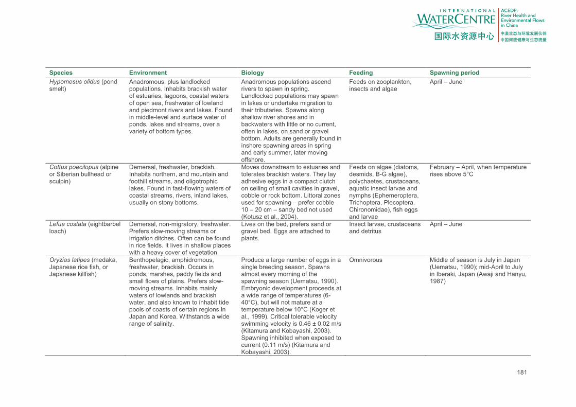
181


Hypomesus olidus (pond smelt)

Anadromous, plus landlocked populations. Inhabits brackish water of estuaries, lagoons, coastal waters of open sea, freshwater of lowland and piedmont rivers and lakes. Found in middle-level and surface water of ponds, lakes and streams, over a variety of bottom types.

Anadromous populations ascend rivers to spawn in spring. Landlocked populations may spawn in lakes or undertake migration to their tributaries. Spawns along shallow river shores and in backwaters with little or no current, often in lakes, on sand or gravel bottom. Adults are generally found in inshore spawning areas in spring and early summer, later moving offshore.

Feeds on zooplankton, insects and algae

April – June

Cottus poecilopus (alpine or Siberian bullhead or sculpin)

Demersal, freshwater, brackish. Inhabits northern, and mountain and foothill streams, and oligotrophic lakes. Found in fast-flowing waters of coastal streams, rivers, inland lakes, usually on stony bottoms.

Moves downstream to estuaries and tolerates brackish waters. They lay adhesive eggs in a compact clutch on ceiling of small cavities in gravel, cobble or rock bottom. Littoral zones used for spawning – prefer cobble 10 – 20 cm – sandy bed not used (Kotusz et al., 2004).

Feeds on algae (diatoms, desmids, B-G algae), polychaetes, crustaceans, aquatic insect larvae and nymphs (Ephemeroptera, Trichoptera, Plecoptera, Chironomidae), fish eggs and larvae

February – April, when temperature rises above 5°C

Lefua costata (eightbarbel loach)

Demersal, non-migratory, freshwater. Prefers slow-moving streams or irrigation ditches. Often can be found in rice fields. It lives in shallow places with a heavy cover of vegetation.

Lives on the bed, prefers sand or gravel bed. Eggs are attached to plants.

Insect larvae, crustaceans and detritus

April – June

Oryzias latipes (medaka, Japanese rice fish, or Japanese killfish)

Benthopelagic, amphidromous, freshwater, brackish. Occurs in ponds, marshes, paddy fields and small flows of plains. Prefers slow-moving streams. Inhabits mainly waters of lowlands and brackish water, and also known to inhabit tide pools of coasts of certain regions in Japan and Korea. Withstands a wide range of salinity.

Produce a large number of eggs in a single breeding season. Spawns almost every morning of the spawning season (Uematsu, 1990). Embryonic development proceeds at a wide range of temperatures (6-40°C), but will not mature at a temperature below 10°C (Koger et al., 1999). Critical tolerable velocity swimming velocity is 0.46 ± 0.02 m/s (Kitamura and Kobayashi, 2003). Spawning inhibited when exposed to current (0.11 m/s) (Kitamura and Kobayashi, 2003).

Omnivorous Middle of season is July in Japan (Uematsu, 1990); mid-April to July in Iberaki, Japan (Awaji and Hanyu, 1987)

182


Coilia ectenes Clupeiformes: Engraulidae (Coilia nasus)

(estuarine tapertail anchovy, lake anchovy, Japanese grenadier anchovy)

Pelagic-neritic, anadromous, freshwater, brackish, marine. Occurs in coastal waters, estuaries and reaching up to middle parts of rivers, able to tolerate freshwater. Lives in water of moderate turbidity. Goes to the deep water areas of rivers at night. Landlocked populations also occur in Lake Tai – they live their entire life in freshwater (Yang et al., 2006). A freshwater resident stock inhabits the middle and lower reaches of the Yangtze River, in both the main stem and connected lakes (Li et al., 2007).

Spawns around three times in a lifetime, with spawning occurring in-between reeds. In the Chikugo River, Japan, the fishes migrate about 15 km upstream and spawn in freshwater, the spherical eggs floating down and hatching near the river mouth. Reaches sexual maturity at 1–2 years of age (Zhao et al., 2007). Mature individuals migrate upriver and spawn in the lower and middle reaches of the Yangtze River and other coastal rivers in China (Ma et al., 2010). Spawning also occurs in the estuary, but females spawning in the estuary are smaller (and therefore less valuable for population recruitment) than those migrating to freshwater to spawn (Li et al., 2007). Also spawn in lakes adjacent to the Yangtze River, including Poyang and Taihu Lakes, where anadromous migrations have ceased and the fish have taken up permanent residence (Ma et al., 2010). Spawning velocity and depth requirements are 0.7-1.4 m/s and 1-2 m, with a maximum of 1 m/s for the upstream spawning migration (Jiang et al., 2010). Spawning activity is correlated with increased river discharge (Zhong and Power, 1996).

Planktivorous In China lays eggs from April to October, breeding once every year (Zhao et al., 2007). Peak breeding time is late spring and early summer (Li et al., 2007). In Ariake Sound, Japan it breeds from May to August. From early February to the end of April adults move upstream into the Yangtze River and spawn in affiliated lakes in the Yangtze’s middle and lower reaches (Ma et al., 2004; Li et al., 2007). In China, landlocked lake populations may spawn later than anadromous populations (Li et al., 2007; Ma et al., 2010). Spawning migration: Apr – Jun upstream; Jul – Oct downstream, spawning Jun – Aug (Jiang et al., 2010).

183


Hucho taimen (taimen) Benthopelagic, potamodromous, freshwater. Inhabits piedmont and montane cold rivers with high oxygen concentrations. Prefers to live in deeper holes with slow current for periods of reduced activity (day time, winter), but also lower reaches, estuaries, cold lakes and reservoirs. Both juveniles and adults are territorial. Adults frequently occur within their own restricted territory (deep holes below rapids and waterfalls, confluence of small tributaries, below bridge pillar or large rocks, bank excavations), which they abandon only for foraging and spawning. Taimen prefer fast moving rivers (MTP, 2008).

A very large fish, having once attained a maximum of over 2 m and 100 kg (MTP, 2008). It breeds in shallow places with fast current on pebble bottom, immediately downstream of large deep pools, often in small river tributaries. Usually undertakes upriver migration for spawning in the upper reaches of tributaries [usually side tributaries of about 0.5-1.5 m in depth (MTP, 2008)]. Can overcome quite high obstacles while migrating to spawning sites. Eggs hatch after 28-38 days. Alevins stay in gravel until yolk sac is absorbed after 10-15 days while young first remain near spawning site, then move downstream. Larger immature individuals of 2-4 years of age live in same sites as adults but separately below groups of adults or in smaller holes. Juveniles occur in fast-flowing waters, prey on drifting invertebrates and shift to fish diet after 1-3 years. Life span reaches up to about 20 years. In north-central Mongolia, movement observed to be greatest in May and June (spawning and post-spawning period) with another peak period of movement in September and October (water temperature cooling) (Gilroy et al., 2010). Taimen migrations of 10-40 km have been reported, but large fish do not migrate more than 1-2 km per year (MTP, 2008).

Carnivorous, feeding on smaller fishes and also amphibians, small mammals and birds (MTP, 2008)

April or May (MTP, 2008). The time of spawning depends on water temperature. The total duration of the spawning season at any given location is reported at between 7-14 days (MTP, 2008).

184


Cyprinus carpio carpio Linnaeus (common carp)

Benthopelagic, potamodromous, freshwater, brackish. Inhabit warm, deep, slow-flowing and still waters such as lowland rivers and large, well vegetated lakes. Hardy and tolerant of a wide variety of conditions but generally favour large water bodies with slow flowing or standing water and soft bottom sediments. Thrive in large turbid rivers. Lethal turbidity level approximately 165 g/L. Moderately tolerant of low DO levels, may gulp atmospheric oxygen at very low DO levels.

Most active at dusk and dawn. Carp are mainly bottom dwellers but search for food in the middle and upper layers of the water body. Spawns along shores or in backwaters. Adults often undertake considerable spawning migration to suitable backwaters and flooded meadows. Eggs sink and adhere to rooted vegetation or other firm substrates. Larvae survive only in very warm water among shallow submerged vegetation. Adults prefer depth >1.5 m and 0.1-0.8 m/s; for spawning, shallow water and velocity <0.3 m/s is preferred (Jiang, 2010).

Omnivorous, with a high tendency towards the consumption of animal food, such as water insects, larvae of insects, worms, molluscs, and zooplankton. Also organic detritus and macrophytes.

April – June when water temperature is 17-18°C and ceases at 27°C. Asian strains start to spawn when the ion concentration of the water decreases abruptly at the beginning of the rainy season.

Ctenopharyngodon idellus

(grass carp) Demersal, potamodromous, freshwater. Occurs in lakes, ponds, pools and backwaters of large rivers, preferring large, slow-flowing or standing water bodies with vegetation. Tolerant of a wide range of temperatures from 0° to 38°C, and salinities to as much as 10 ppt and oxygen levels down to 0.5 ppm. Prefers clear water but can tolerate high turbidity.

Normally dwell in mid-lower layer of the water column. It is a semi-migratory fish; adults migrate to the upper reaches of major rivers to propagate. Flowing water and changes in water level are essential environmental stimuli for natural spawning. Spawning grounds are usually located in river reaches characterized by turbulent or whirlpool-like flow, often in the vicinity of islands or stream junctions (Yih and Liang, 1964). Spawns on riverbeds with very strong current, in the range 0.7-1.8 m/s, following a rise in water level of as little as 10-15 cm (Shireman and Smith, 1983, p. 29). Semi-buoyant eggs drift 50-180 km before hatching (Shireman and Smith, 1983, p. 12)

Higher aquatic plants and submerged grasses; takes also detritus, insects and other invertebrates.

Movement begins April – July (Jiang et al., 2010), when water temperature rises to 15-17°C (Shireman and Smith, 1983, p. 29), and spawning begins at 18°C.

185


Hypophthalmichthys nobilis (bighead carp)

Benthopelagic, potamodromous, freshwater. Lives in rivers with marked water-level fluctuations, overwinters in middle and lower stretches. Able to tolerate water temperatures of 0.5-38°C. Can tolerate high turbidity.

Forages in shallow (0.5-1.5 m deep) and warm (> 24°C) backwaters, lakes and flooded areas with slow current. Bottom feeding fish. Undertakes long distance upriver migration at start of a rapid flood and water-level increase (in April-July depending on locality). Spawning grounds are usually located in river reaches characterized by turbulent or whirlpool-like flow, often in the vicinity of islands or stream junctions (Yih and Liang, 1964). Breeds in very deep, very turbid and warm water > 18°C (usually 22-30°C), with high current (1.1-1.9 m/s) and high oxygen concentrations. Spawns in upper water layer or even at surface during floods. Spawning ceases if conditions change and resumes again when water level increases. After spawning, adults migrate for foraging habitats. Semi-buoyant eggs are laid that are maintained in suspension by turbulence. The eggs are thought to die if they sink to the bottom. Larvae drift downstream and settle in floodplain lakes, shallow shores and backwaters with little or no current. During autumn-winter, when temperature drops to 10°C, juveniles and adults form separate large schools and migrate downstream to deeper places in main course of river to overwinter.

Mainly zooplankton, but also takes algae as food

April – July (peak in May) depending on locality when temperature exceeds 18°C (usually 22-30°C)

acedp hydrology indicator report

Documents