achievement gap between indigenous and non … · achievement gap between indigenous and...
TRANSCRIPT

Achievement Gap between Indigenous and Non-Indigenous
Children in PeruAn Analysis of Young Lives Survey Data
Irma Arteaga and Paul Glewwe
Wo
rkin
g P
aper
JUNE 2014
130
www.younglives.org.uk


Wo
rkin
g P
aper
JUNE 2014
130
www.younglives.org.uk
Achievement Gap between Indigenous and Non-Indigenous
Children in PeruAn Analysis of Young Lives Survey Data
Irma Arteaga and Paul Glewwe

Achievement Gap between Indigenous and Non-Indigenous Children in Peru: An Analysis of Young Lives Survey Data
Irma Arteaga and Paul Glewwe
First published by Young Lives in June 2014
© Young Lives 2014 ISBN: 978-1-909403-44-4
A catalogue record for this publication is available from the British Library. All rights reserved. Reproduction, copy, transmission, or translation of any part of this publication may be made only under the following conditions:
• withthepriorpermissionof thepublisher;or
• withalicencefromtheCopyrightLicensingAgencyLtd., 90 Tottenham Court Road, London W1P 9HE, UK, or from another national licensingagency;or
• underthetermssetoutbelow.
This publication is copyright, but may be reproduced by any method without fee for teaching or non-profit purposes, but not for resale. Formal permission is required for all such uses, but normally will be granted immediately. For copying in any other circumstances, or for re-use in other publications, or for translation or adaptation, prior written permission must be obtained from the publisher and a fee may be payable.
Printed on FSC-certified paper from traceable and sustainable sources.
Young Lives, Oxford Department of International Development (ODID), University of Oxford,
Queen Elizabeth House, 3 Mansfield Road, Oxford OX1 3TB, UK
Tel: +44 (0)1865 281751 • E-mail: [email protected]
Funded by

ACHIEVEMENT GAP BETWEEN INDIGENOUS AND NON-INDIGENOUS CHILDREN IN PERU: AN ANALYSIS OF YOUNG LIVES SURVEY DATA
i
Contents Summary ii
The Authors iii
Acknowledgements iii
1. Introduction 1
2. Literature review 1
3. Education and Peru’s indigenous population 4
4. Data and variables used 5
5. Methodological framework 8
6. Empirical approach 9
7. Results 14
8. Conclusion and policy implications 21
References 22
Appendix 26

ACHIEVEMENT GAP BETWEEN INDIGENOUS AND NON-INDIGENOUS CHILDREN IN PERU: AN ANALYSIS OF YOUNG LIVES SURVEY DATA
ii
SummaryIn Peru, indigenous children obtain lower scores on academic tests, on average, than non-
indigenous children. In this study, we investigate whether a test score achievement gap is found by the age of 5 and whether this gap increases by the age of 8. While the literature has focused on the underlying family and children determinants of achievement gaps, we use an
extension of the Oaxaca-Blinder technique to include community sorting effects and heterogeneity in community impact effects. Using the 2001 cohort of the Young Lives longitudinal survey for Peru, our results show that at the age of 5, indigenous children are far
behind their non-indigenous counterparts in Spanish vocabulary (as measured by the PPVT), but less far behind in maths. Over the first three years of school, however, indigenous children lose substantial ground relative to non-indigenous children, increasing the average
gap to 0.49 standard deviations (of the distribution of test scores) in maths and 0.66 in vocabulary. Our results suggest not only that parental education and a child’s health are important determinants of the gap for maths and vocabulary, as previously found in the
literature; but also that the vocabulary gap is due in part to community effects. The pathways considered yield valuable information for policymakers who are interested in developing policies to improve student learning among indigenous groups. These pathways are
important for human capital formation and could potentially have long-term impacts on educational attainment and poverty in Peru.
JEL classification: I20; J15; H75; O15
Keywords: Child development; Cognitive skills; Test scores; Indigenous – non-indigenous
gap; Peru

ACHIEVEMENT GAP BETWEEN INDIGENOUS AND NON-INDIGENOUS CHILDREN IN PERU: AN ANALYSIS OF YOUNG LIVES SURVEY DATA
iii
The Authors Irma Arteaga is an Assistant Professor at the University of Missouri. She has a Master’s
degree in Public Policy and a PhD in Applied Economics from the University of Minnesota. Her research interests include development economics, programme evaluation of early childhood interventions, and safety net programmes and their impacts on food insecurity and
the health of children. She is currently investigating the effects of a conditional cash transfer programme on child malnutrition and years of schooling in Panama. In addition to that, she is studying the effect of different early childhood interventions on food insecurity, using US
longitudinal datasets.
Paul Glewwe is a Distinguished McKnight University Professor in the Department of Applied
Economics at the University of Minnesota, where he teaches econometrics, microeconomics and microeconomic analysis of economic development. His research focuses on education in
developing countries, especially the factors that determine academic outcomes in primary and secondary schools. He also conducts research on malnutrition, inequality and poverty in developing countries. He has conducted research on Brazil, China, Côte d’Ivoire, Ghana,
Honduras, Jamaica, Jordan, Kenya, Madagascar, Malaysia, Morocco, Peru, the Philippines, Sri Lanka and Vietnam. Before joining to the University of Minnesota in 1999, he was a senior research economist at the World Bank.
Acknowledgements We are grateful to Raj Darolia and Caine Rolleston for critical readings of previous drafts. We
also want to thank Ray Zuniga for his diligent assistance with our project.
About Young Lives
Young Lives is an international study of childhood poverty, following the lives of 12,000 children in 4 countries (Ethiopia, India, Peru and Vietnam) over 15 years. www.younglives.org.uk
Young Lives is funded from 2001 to 2017 by UK aid from the Department for International Development (DFID), co-funded by the Netherlands Ministry of Foreign Affairs from 2010 to 2014, and by Irish Aid from 2014 to 2015.
The views expressed are those of the author(s). They are not necessarily those of, or endorsed by, Young Lives, the University of Oxford, DFID or other funders.


ACHIEVEMENT GAP BETWEEN INDIGENOUS AND NON-INDIGENOUS CHILDREN IN PERU: AN ANALYSIS OF YOUNG LIVES SURVEY DATA
1
1. Introduction Peru has the largest indigenous population in Latin America, and children in these
indigenous families struggle with an achievement gap, relative to their non-indigenous peers, that is significant, persistent and poorly understood. In Peru, the indigenous population
consists of 8.5 million people who speak 67 different indigenous languages, accounting for approximately 30 per cent of the total population. In Peru’s rural areas, where most indigenous families live, children’s maths and vocabulary test scores are among the lowest in
Latin America, including Guatemala, Mexico, Chile and Bolivia. Prior research in Latin America shows that these gaps persist even after controlling for socioeconomic status indicators (Sakellario 2008; Marshall 2009; McEwan and Trowbridge 2007; Hernandez-
Zavala et al. 2006; McEwan 2004).
So far, researchers have not explained what has caused this achievement gap to occur, and
why it persists. In some studies, as much as 50 per cent of the achievement gap between indigenous and non-indigenous students is left unexplained. Prior research finds that family
and parental influences are important, as well as the quality of schools, but the results are inconsistent and unsatisfying. Data from Chile suggest that schools explain a large portion of the gap (McEwan 2008), but data from Mexico and Guatemala show that school effects are
not as important as family factors and that together they still do not fully explain the gap (Hernandez-Zavala et al. 2006). Also, while the literature recognises that child health is crucial for explaining children’s achievement gaps (Glewwe and Miguel 2008; Marshall
2009), prior studies have not included child health.
In short, while parental education, parental behaviour, the quality of schools and child health
have all been suggested, no comprehensive attempt has been made in Latin America to explain the achievement gap using all of these factors at once, while controlling for
demographics and socioeconomic status. For example, researchers have examined the effects of parental behaviour (e.g. parent helps child with homework, parent plays with child), but data limitations precluded them from separating those effects from the effect of
socioeconomic status.
This paper reviews the literature on explanations for ethnic achievement gaps in different
countries, and uses an extension of the Oaxaca-Blinder decomposition method to account for community effects. Given the very detailed information collected in the Young Lives surveys, we are able to use a rich array of covariates to control for family background
characteristics. This allows us to better understand the experience of Peruvian children and to discuss the issue of the ethnic achievement gap in Peru in a comprehensive study that yields important policy insights for the Peruvian case.
2. Literature review The education literature has established that, in addition to basic socioeconomic factors and
genetic endowments, family influences are important contributors to cognitive development. However, this research has been largely conducted in the United States, leaving cognitive
production and achievement gaps among Latin American children much less well understood.

ACHIEVEMENT GAP BETWEEN INDIGENOUS AND NON-INDIGENOUS CHILDREN IN PERU: AN ANALYSIS OF YOUNG LIVES SURVEY DATA
2
For example, research on children in the United States shows that breastfeeding, length of
breastfeeding, and whether a child attended an early childhood programme have significant effects on cognitive development (Currie 2009; Neidell 2000). Similar research shows that
having an educationally supportive home also promotes cognitive achievement (Driessen et al. 2005; Fishel and Ramirez 2005). A study of the test score gap between black and white students in the United States finds that differences in ‘household’ inputs explain 10–20 per
cent of the test score gap and that differences in maternal AFQT scores1 (a proxy of ability) explain as much as 50 per cent of that gap (Todd and Wolpin 2007).
Family characteristics and parental behaviour and practices also play an important role in a
child’s cognitive achievement. For example, an investigation using data from the US National
Institute of Child Health and Human Development (NICHD) Study of Early Child Care and Youth Development shows that, among third-graders, a rough measure of ‘maternal sensitivity’ explains almost one-third of the gap in test scores between black and white
students. Maternal sensitivity was measured by mother–child structured play interaction during semi-structured 15-minute observations when children were 6 and 15 months of age. Maternal sensitivity was composed of three sub-scales: supportive presence, respect for the
child’s autonomy and hostility (Murnane et al. 2006).
Outside of the household, researchers have also examined school and teacher quality as
critical elements. Cook and Evans (2000) attribute the decrease in the test score achievement gap between black and white students in the United States between the 1970s
and 2000 to family factors, as well as to school and teacher quality. Using the Oaxaca-Blinder decomposition technique and data from the National Assessment of Education Progress, they found that, together, convergence in family factors and school quality
explained only 25 per cent of the convergence in test scores. They concluded that to better explain the achievement gap we need more detailed variables for parental education and school quality, but that that would still leave out important elements such as health and
parenting attitudes.
In Latin America, the findings are fewer and less clear, mainly due to the lack of appropriate
datasets. Specifically, there is little research on how parental behaviour affects educational outcomes. In addition, findings on the relative importance of family characteristics, school factors and parenting quality are mixed. For example, analysis of data from the National
Census for Student Achievement (SIMCE) in Chile shows that school effects have a large impact on the test score gap between indigenous and non-indigenous students (McEwan 2008), while a family’s socioeconomic status had only a small effect. This study used a
differences-in-differences method and a modified Oaxaca-Blinder decomposition method to examine maths and Spanish scores for 8-year-olds in 1997 and 2001.
Meanwhile, other studies find that the achievement gap is difficult to explain through either
family factors, school factors, or both. An analysis of data on test scores in Mexico and
Guatemala shows that family and school factors leave between 25 per cent (Mexico) and 59 per cent (Guatemala) of the language gap unexplained and between 32 per cent (Mexico) and 45 per cent (Guatemala) of the mathematics gap unexplained (Hernandez-Zavala et al.
2006).
1 Armed Forces Qualifying Test. The test was administered as part of the research.

ACHIEVEMENT GAP BETWEEN INDIGENOUS AND NON-INDIGENOUS CHILDREN IN PERU: AN ANALYSIS OF YOUNG LIVES SURVEY DATA
3
As in the United States, parenting behaviour or practices may explain some of the remaining
gap. There is certainly strong evidence that parenting practices help determine children’s cognitive skills (James-Burdumy 2005; Kimmel and Connelly 2007; Paxson and Schady
2007). However, research on Latin American children has focused more on health on parenting practices, partly in response to research in the developed countries that highlights the importance of health for a child’s cognitive development. Research on children in the
United States shows that a well-nourished child pays better attention in class, focuses, concentrates and gets better grades (Currie 2009). The role of health is even more important in a developing country such as Peru, where poor early childhood nutrition is harder to
remedy and may cause lasting cognitive deficiencies that would be difficult or impossible to remedy in later years (Alderman et al. 2001).
As a result, health has been more of a focus in the literature on Latin America; but it has
been largely theoretical because data limitations have prevented most empirical work from
including child health as a determinant of the test score gap between indigenous and non-indigenous students. Including children’s health requires measurement of nutrition and maternal health during the first years of a child’s life, when nutrition is thought to have the
greatest influence on cognitive development. But, there are few datasets available that include information on early nutrition and maternal health as well as test scores that measure cognitive development. Also, many datasets have no health data at all, because health
encompasses a broad range of factors and is notoriously difficult to measure.
This paper advances the literature by being one of the first of its kind to explicitly examine the
achievement gap between Quechua and Aymara (indigenous) speakers on the one hand and Spanish (non-indigenous) speakers on the other in Peru. Despite the fact that Quechua
people are the largest indigenous group in Peru and the Quechua language is Peru’s second official language, until recently there have been few datasets available on the performance of Quechua-speaking students. This study uses a new, unusually rich dataset containing
information on indigenous children, their caregivers and family background and community characteristics.
This paper is also the first of its kind to combine data on parenting behaviour and child health
to help explain the ethnic (indigenous vs. non-indigenous) achievement gap. By using Round 3 data from the Young Lives study, this paper will comprehensively compare children by
linguistic background, and measure the effects of parental education, family factors, child health and geographic location on their cognitive achievement. The Young Lives dataset provides longitudinal data for almost 1,800 Peruvian children who were approximately 1 year
old in 2002, 5 years old in 2006, and 8 years old in 2009.
This paper also applies the extension of the Oaxaca-Blinder decomposition proposed by
Glewwe et al. (2013), which adds two additional effects to that decomposition: community sorting effects and differential community impact effects. The former measures the extent to
which the gap is due to indigenous children living in different communities. The latter indicates whether the gap is due to the fact that non-indigenous children learn more than indigenous children in the same community. This is the first time that this method has been
used to decompose differences in educational outcomes between indigenous and non-indigenous children.

ACHIEVEMENT GAP BETWEEN INDIGENOUS AND NON-INDIGENOUS CHILDREN IN PERU: AN ANALYSIS OF YOUNG LIVES SURVEY DATA
4
3. Education and Peru’s indigenous population Peru is a lower-middle-income country that is typical of Latin American countries in most ways but unusual in two important respects that are relevant here: its high number of
indigenous people and its high level of child malnutrition. About 30 per cent of Peru’s population is indigenous, which we define here in terms of the language learned at home. According to Peru’s census of 2007, 83 per cent of the indigenous population speak
Quechua, 11 per cent speak Aymara, 2 per cent speak Ashaninka, and 4 per cent speak other indigenous languages (INEI 2008).
According to Vásquez-Huamán et al. (2008) there are three main ways to define ‘indigenous’:
by mother tongue, which is objective; self-identification, which is subjective; or through
territory, race, religion or clothing, all of which are also subjective. We choose to define indigenous and non-indigenous based on mother tongue because this definition is both objective and the most commonly employed definition in Latin America. Bolivia, Ecuador,
Colombia, Honduras, Mexico, Paraguay and others all use mother tongue to define indigenous.
Overall, Peru appears similar to other Latin American countries. Peru’s GDP per capita in
2010 was US$5,205, just 11 per cent of that of the United States (IMF 2011) but not atypical
for Latin America. An estimated 31 per cent of Peruvians live below the Peruvian Government’s official poverty line (INEI 2012). Yet relative to its Latin American neighbours, Peru appears somewhat less poor; an estimated 4.9 per cent of the population live on
US$1.25 per day and less and 12.7 per cent live on two dollars per day or less (World Bank 2010).
Education and health indicators for Peru are roughly on a par with those of other Latin
American countries. Net primary school enrolment in Peru for males and females is 96 per cent and 97 per cent, respectively, while the averages for the Latin American region are 94
per cent and 95 per cent, respectively. Likewise, net secondary school enrolment in Peru for both males and females is 75 per cent, compared to 69 per cent and 74 per cent for the Latin American region. Improving educational outcomes for those who are in school, however,
remains a challenge; 73.5 per cent of Peruvian children tested were at or below the lowest level for mathematics proficiency in the 2009 PISA learning assessments of 15-year-old children in 62 countries, and 64.8 per cent of those tested were at or below the lowest level
for reading proficiency (OECD 2010).
Infant and child mortality are slightly lower in Peru than in the rest of the Latin American and
Caribbean region. According to the World Bank, in 2011 the infant mortality rate in Peru per 1,000 live births was 14, compared to an average of 19 for the Latin America and Caribbean
region. By the age of 5, the child mortality rate of 18 per 1,000 live births in Peru approaches the (average) rate of 19 for the region.
However, on some measures of child nutrition, Peru fares much worse. Thirty per cent of
children under 5 have low height-for-age (stunting), a figure that is far above the Latin
American average of 16 per cent (UNICEF 2009). Moreover, the incidence of low birth weight is 10 per cent, slightly higher than the Latin American average of 9 per cent.

ACHIEVEMENT GAP BETWEEN INDIGENOUS AND NON-INDIGENOUS CHILDREN IN PERU: AN ANALYSIS OF YOUNG LIVES SURVEY DATA
5
And, when one looks more closely at data for indigenous versus non-indigenous children in
Peru, some important differences emerge. The Peruvian National Institute of Statistics reports that the enrolment rate of children aged 6–16 years that are Spanish-speaking is 96
per cent, while the rate for indigenous children is 88 per cent. Further, of all school-age (5–18 years old) indigenous children, 29 per cent do not actually go to school and 73 per cent are at least one grade level behind what is appropriate for their age.2
Peru recognises the importance of addressing the educational gap between its indigenous
and non-indigenous children, but political and bureaucratic obstacles have limited its ability to institute policy changes that reduce the achievement gap. In the 1970s the Ministry of Education initiated a National Policy of Bilingual Education and created the National Division
of Intercultural and Bilingual Education (DINEBI), charged with finding ways to educate indigenous people better. Since then, few meaningful advances have been made, largely because the DINEBI has had to compete for resources with other national priorities and with
the agendas of the larger and more powerful Ministry of Education and the Vice Ministries of Educational Management and Institutional Management. For example, the DINEBI still does not have the capacity to hire new teachers or to approve a bilingual curriculum for the future
(Castillo et al. 2008). Peru has had some success creating intercultural bilingual schools, but according to the Peruvian Ministry of Education, in 2008 only 35 per cent of the rural bilingual population attended an intercultural bilingual school.
4. Data and variables used
4.1. Data
Young Lives is a longitudinal study that collects data from about 12,000 children in Ethiopia,
India, Peru and Vietnam in order to investigate the changing nature of childhood poverty. The Young Lives study tracks two cohorts of children in each country over a 15-year period. Both cohorts have three rounds of data, collected in 2002, 2006 and 2009 (with a fourth round
collected in late 2013 / early 2014 but not yet available for analysis). The Younger Cohort consists of children who were between 6 and 18 months of age in 2002, and the Older Cohort consists of children who were between 7.5 and 8.5 years old in that year.
This study uses data for the Younger Cohort of children in Peru, for which two rounds of data
(2006 and 2009) are available that include measures of cognitive development. The complete panel dataset for the Peru Younger Cohort includes 1,823 children, selected through multi-stage, stratified, random sampling. However, we exclude 69 children from our
analysis because of missing data. In most cases, the missing values were because the father was not present in the household at the time of the interview or the parents did not answer questions on time spent with children. A comparison of the mean characteristics and t-tests
for the full sample of children and the sub-sample of children used in the analysis suggests that any differences between the two groups are very small and not statistically significant (see Table A3 in the Appendix). The sub-set we use represents the whole country of Peru; it
2 Children start school at the age of 6 in Peru but may attend kindergarten from the age of 5. Young people in rural areas finish
secondary school at 18.
ACHIEVEMENT GAP BETWEEN INDIGENOUS AND NON-INDIGENOUS CHILDREN IN PERU: AN ANALYSIS OF YOUNG LIVES SURVEY DATA
6
covers 20 districts that are part of 18 states in Peru,3 In the sample, 35 per cent of the children live near the coast, 50 per cent in the mountains and 15 per cent in the jungle. The Young Lives study provides information on household and child characteristics, and detailed
caregiver records, as well as children’s scores in a quantitative/maths test and the Spanish version of the Peabody Picture Vocabulary Test (PPVT).
Given that the Young Lives study is based on a longitudinal survey, it is important to consider
the potential for attrition bias. Such bias may occur if attrition is non-random and leads to a
situation where unobserved characteristics that are correlated with attrition are also correlated with the outcomes of interest. Outes-Leon and Dercon (2008) analysed Rounds 1 and 2 of data for the four Young Lives countries and found a 3.5 per cent attrition rate for the
Peru sample, which is low compared to other longitudinal studies in developing countries. The authors also applied BGLW4 tests for attrition bias and found attrition was overwhelmingly random and unlikely to lead to significant biases.
4.2. Variables used in the analysis
The key outcome of interest in this study is cognitive ability, which the Young Lives study
measures by a child’s scores in the quantitative (maths) test and in the PPVT. These tests
were conducted in Rounds 2 and 3, so our analysis is limited to those two rounds. In Round 2, the quantitative test used was the Cognitive Development Assessment – Quantitative, or CDA-Q, which was developed for children 4.5–5.5 years of age. The CDA-Q consists of 15
items. For each item the child is shown a picture and asked a question. The child is asked to choose the best answer from three or four possible choices; for example, ‘Look at the plates of cupcakes; point to the plate that has the fewest cupcakes’. The raw score is calculated as
the number of correct answers, where the child scores one point for each correct answer and zero points for incorrect or incomplete answers.
In Round 3, a two-part quantitative assessment was used. The first part consisted of nine
questions, where the survey researcher showed the child a series of cards and asked him or her to answer orally; for example, ‘Please put your finger on number 21,’ or ‘Which number
should be in the blank space?’ In part two, children were tested on maths computing. The survey researcher gave each child a test booklet and explained the instructions to him or her. The child then had 12 minutes to read and write down answers to 20 basic arithmetic
questions.
In both rounds, Young Lives used the Spanish version of the PPVT (TVIP in Spanish), which
is a test of receptive vocabulary that has been widely used in Latin America as a general measure of cognitive development (Bernal 2008; James-Burdumy 2005; Paxson and Schady
2007; Schady 2006; Umbel et al. 1992). During the test, children were asked to select from among four pictures the one that best represented the meaning of a word the interviewer presented to them orally. During the test, 125 questions are presented, arranged in ten
groups. Each group corresponds to items that children of a certain age could be expected to be proficient in. Thus, the first questions are targeted at 3–4-year-old children, the next group at 5-year-old children, and so on. Of course, it is unlikely that 8-year-old children will answer
all 125 questions correctly, but some children will be able to recognise words that are far
3 One district was randomly chosen within 17 of Peru’s 18 departments. In the 18th and largest department, Lima, three districts
were selected. The reason is that almost one-third of the population in Peru lives in Lima.
4 BGLW stands for Becketti, Gould, Lilliard and Welch (1988) test for selection on observables.

ACHIEVEMENT GAP BETWEEN INDIGENOUS AND NON-INDIGENOUS CHILDREN IN PERU: AN ANALYSIS OF YOUNG LIVES SURVEY DATA
7
beyond the expectations for their age. For this reason, the test uses a continuation rule for each set; moving on to the next set requires three or more correct answers in the previous set.
Test items for the Spanish PPVT have been selected for their universality and
appropriateness to Hispanic communities and have been widely used both in Latin American
countries and with Spanish-speaking children in the United States (Paxson and Schady 2007; Rosenzweig and Wolpin 1994). During Rounds 2 and 3 of the Young Lives study, the PPVT was available in Spanish, Quechua and Aymara, the most commonly spoken
languages in Peru.5 The PPVT items have been validated in Spanish, but not in Quechua and Aymara, because these populations live only in Peru and Bolivia and the sample sizes are not large enough for validation.
To capture socioeconomic characteristics, we use data from the Young Lives study on the
natural logarithm of annual household expenditure, father’s education, and mother’s education. To calculate the annual household expenditure we summed all the expenses reported by the head of the household during the year, including items bought on weekly,
monthly and annual bases, as well as payments for utilities and services. The education of parents is given in completed years.
To account for parental behaviour contributing to the development of their child, we use data
from the Young Lives study to construct six variables: the natural logarithm of education expenditure; months the child has spent in day care since he or she was born; months of
breastfeeding; month of mother’s first prenatal visit; whether a parent helps the child with homework; and whether a parent plays with the child. We initially intended to use two additional measures – number of months in preschool and hours per week spent in
preschool – but they turned out to be highly correlated with expenditure on education so we dropped them from the analysis.
To measure early childhood nutrition, we use a child’s height-for-age z-score, because the
literature finds that this is the best single indicator of cumulative nutritional status for infants
and children (McKee and Todd 2009; Hoddinott 2012; Glewwe et al. 2001). This study instruments a child’s height-for-age when he or she was tested using the same child health indicator as when the child was 1 year old. Instrumental variable (IV) estimation is used for
two reasons. First, ordinary least squares (OLS) estimates of the impact of child nutrition on cognitive skills are likely to be biased because a child’s nutritional status and his or her educational progress may both be determined by unobserved parental actions that reflect
tastes regarding their child’s human capital formation, leading to omitted variable bias. Second, a child’s height-for-age z-score may measure his or her nutritional status with random errors (there is variation in height and weight even among healthy children, which
implies that this z-score can be a noisy measure of child’s nutritional status). Height-for-age in Round 1 is unlikely to be correlated with parental actions in the first one to two years of life that depend on a child’s ability to learn because that child’s ability to learn is unlikely to be
apparent at the age of 6–18 months; thus, using it as an instrument for our child health measure at Round 2 and Round 3 will address the first problem. It is also a good ‘second measurement’ of height-for-age in later rounds and thus can be used as an instrument to
address bias due to measurement error.
5 Spanish and Quechua are both official languages in Peru. One possible explanation for the widening gap in test scores between
indigenous and non-indigenous children is that some indigenous students who took the test in Quechua or Aymara in Round 2 (2006) took it in Spanish in Round 3 (2009), which may have reduced their test scores. However, only 88 students did so between
the two rounds. More importantly, when these 88 students are dropped from the analysis, the results are essentially unchanged.

ACHIEVEMENT GAP BETWEEN INDIGENOUS AND NON-INDIGENOUS CHILDREN IN PERU: AN ANALYSIS OF YOUNG LIVES SURVEY DATA
8
5. Methodological framework The process by which cognitive skills (e.g. literacy and numeracy) are learned depends on
many factors and can be depicted as a mathematical relationship. These relationships can be very flexible, allowing for almost any learning process. Yet even when an education
production function exists, there is no guarantee that one can estimate it.
A simple production function can be used to depict the relationship between cognitive
achievement (A) and the set of variables that act as inputs into the production process. The most important input variables are years of schooling (S), school and teacher characteristics
(Q), child characteristics (C), family characteristics (F), and educational inputs purchased by parents (I):
A = a(S, Q, C, F, I) (1)
The first task of this paper is to estimate the achievement production function depicted in
equation (1). This production function shows how each factor, such as maternal education, affects academic achievement, holding all other factors constant.
Estimating an achievement production function can be a difficult task. One approach is to
apply linear regression methods to a linear approximation of equation (1). The following linear specification shows each variable in the vectors Q, C, F and I explicitly, and adds an error term:
A = β0 + β1S + βq1Q1 + … + βqJQJ + βc1C1 + …
+ βcKCK + βf1F1 + … βfMFM + βi1I1 + … βiNIN + ε (2)
where there are J school and teacher characteristics, K child characteristics, M family
characteristics and N educational inputs. The error term ε accounts for measurement errors
in A and for deviations of the linear approximation in (2) from the more general non-linear function in (1).
The causal impacts of the observed characteristics on achievement, the β coefficients, can
be consistently estimated by OLS only if the error term (ε) is uncorrelated with all of the observed variables (S, Q, C, F and I). There are three main reasons why ε is very likely to be
correlated with these explanatory variables: omitted variable bias, measurement error bias and sample selection bias.
Omitted variable bias can lead to correlation between observed explanatory variables in
equation (2) and the error term (ε). This occurs when some important explanatory variables
that are not observed, and therefore become part of the error term (ε) of equation (2), are correlated with the observed variables. Here, difficult to observe variables could include teachers’ motivation, headteachers’ management skills, children’s ability and motivation, and
the community environment (e.g. existence of after-school programmes and the nature of labour market opportunities). Given the richness of the Young Lives data, most of the variables in equation (2) can be found in the Peru data. The analysis will control for
unobserved effects on the community environment by using a set of dummy variables for each community. This has the added benefit of controlling for all school and teacher variables, including those that are hard to observe, to the extent that they are common to all
children in the community; these are the Q variables in equations (1) and (2).
ACHIEVEMENT GAP BETWEEN INDIGENOUS AND NON-INDIGENOUS CHILDREN IN PERU: AN ANALYSIS OF YOUNG LIVES SURVEY DATA
9
Measurement error bias may occur when explanatory variables are measured with error. This
is a very common problem for data from both developed and developing countries because some information may be out of date, or because family members do not recall things clearly
or do not know the answer to a question but provide an answer as best they can. Random measurement error typically leads to underestimation of the true impacts of a phenomenon, while non-random measurement error may underestimate or overestimate its true impacts.
This paper will overcome this problem by using IV methods. More specifically, household expenditure per capita will be instrumented using an index of household wealth, and the height-for-age z-score at the age of 5 will be instrumented using the same child health
indicator as when the child was 1 year of age.
Sample selection bias occurs when the data used in an analysis are a non-random sample of
the population of interest. In the case of the Young Lives data for Peru, the data are from a random sample of the population that covers the entire country except the wealthiest 5 per
cent of municipalities, which have very few indigenous children in them. However, there could be bias through attrition, if children in Round 3 are not a representative sample of the original cohort of children surveyed in Round 1 (2002) or Round 2 (2006). Table A3 in the
Appendix shows that this is not the case for the Young Lives data.
6. Empirical approach Estimates of equation (2) can be used to investigate the underlying causes of differences between the test scores of indigenous and non-indigenous children in Peru. To do this, we
use an extension of the Oaxaca-Blinder decomposition, which is commonly used to assess the determinants of earning gaps between two groups of workers (Blinder 1973; Oaxaca 1973). The Oaxaca-Blinder decomposition has recently been used to decompose the
determinants of the racial and ethnic gap in test scores in Peru and Guatemala (Hernandez-Zavala et al. 2006); however, that study used only school data since no household data were available.
The primary objective of this paper is to estimate the factors that contribute to the difference
between the average (mean) test scores of non-indigenous and indigenous primary school students in Peru, which can be denoted by E[ANI] - E[AI]. Glewwe et al. (2013) extended the Oaxaca-Blinder decomposition to account for sorting of students into different schools and
heterogeneity in the impacts of school and teacher characteristics on student learning. We apply this method, but focus on community-level sorting and heterogeneity of impacts. This method decomposes E[ANI] - E[AI] into four components. The first two components have
been widely used in the literature, while the second two, which were first used by Glewwe et al. (2013), have never before been used to decompose differences in educational outcomes between indigenous and non-indigenous children. The components are:
1. Endowment effect: Differences between indigenous and non-indigenous primary school students in the mean values of child and household variables (S, C, F and I);
2. Relative impact effect: Differences between the two groups of students in the
impacts of child and household variables on achievement (differences in βs, βc1 to βcK, βf1 to βfM, and βi1 to βiN);

ACHIEVEMENT GAP BETWEEN INDIGENOUS AND NON-INDIGENOUS CHILDREN IN PERU: AN ANALYSIS OF YOUNG LIVES SURVEY DATA
10
3. Community sorting effect: Differences in where (which communities) indigenous
and non-indigenous students live; and
4. Heterogeneity in community impact effect: Differences between the two groups
of students in the overall impact of community factors (including school factors).
We begin with equation (2). For simplicity, denote all child and household variables (S, C1 to
CK, F1 to FM, and I1 to IN) by the vector X, and denote the associated β parameters (βs, βc1 to βcK, βf1 to βfM, and βi1 to βiN) by the vector . In addition, allow the total impact of community characteristics, which include the school and teacher characteristics Q1 to QJ in equation (2),
to be denoted by αj for each community j. Note that each αj also includes the constant term (β0) in equation (2). These notational changes allow one to express equation (2) as:
Aij = αj + ′Xij + εij (2′)
for student i in community j.
Next, following Glewwe et al. (2013), allow equation (2′) to have different αj and parameters
for indigenous and non-indigenous students. Thus there is one equation for indigenous students and another for non-indigenous students, which can be expressed as:
AijI = αj
I + I′XijI + εij
I (3)
AijNI = αj
NI + NI′XijNI + εij
NI (4)
Equations (3) and (4) are estimated by regressing the test score (A) of child i in community j
on a vector of child and family variables (X) and on a set of dummy variables for each community (which can be denoted by Dj), separately for indigenous and non-indigenous
children. Note that the separate regressions allow each community to have one intercept for indigenous students (αj
I) and another for non-indigenous students (αjNI). The standard errors
will be adjusted for arbitrary forms of heteroskedasticity within communities because
observations within communities are correlated due to their exposure to the same community factors (Wooldridge 2010).
Taking the means of both sides of equation (3) and equation (4), and subtracting the former
from the latter, allows one to write the gap between indigenous and non-indigenous children
as follows:
A NI – A I = Σj=1
20
αjNI D
jNI + NI′ X NI –
Σj=1
20
αjI D
jI – I′ X I (5)
= I′( X NI – X I) + ( NI – I)′ X I + ( NI – I)′( X NI - X I)
+ Σj=1
20
(αjNI
– αjI) D j
I + Σj=1
20
αjNI( D j
NI - D jI)
where the D jNI and D j
I variables indicate the fraction of non-indigenous and indigenous
students, respectively, that are found in each of these 20 communities in the Peru Young Lives data. Note that this expression uses E[εNI] = E[εI] = 0, which is simply a normalisation (for each community, the constant terms αNI and αI are defined so that the means of these
error terms equal zero in each community, which implies that the overall means also equal zero).

ACHIEVEMENT GAP BETWEEN INDIGENOUS AND NON-INDIGENOUS CHILDREN IN PERU: AN ANALYSIS OF YOUNG LIVES SURVEY DATA
11
The decomposition in equation (5) is from the perspective of an indigenous student.6 The
first term, I′( X NI – X I), indicates how much of the test score gap is due to differences in child and family characteristics between non-indigenous and indigenous students, applied to the impact of an indigenous student ( I). The second term, ( NI – I)′X I, adjusts for the
difference between each community’s set of two fixed effects, αjNI - αj
I, which is relevant only for a person with X = 0, to the difference that is appropriate for a person with X = X I; the intuition for this term will be apparent in the discussion below of Figure 1. The third term,
( NI – I)′( X NI – X I), measures the contribution to the test score gap of differences between non-indigenous and indigenous students in the impacts of child and family characteristics on learning, applied to the difference in the average characteristics of non-indigenous and
indigenous students ( X NI – X I). The fourth term, Σj=1
20
(αjNI
– αjI) D j
I, measures how much of
the gap is due to the fact that non-indigenous students may learn more than indigenous students in the same community (and perhaps the same school), even after controlling for
their individual and household characteristics, applied to the distribution of students in the
indigenous communities (the D jI variables). The last term,
Σj=1
20
αjNI( D j
NI – D jI), reflects the
extent to which the gap is due to non-indigenous and indigenous students living in different
communities (as reflected in differences in the D j variables across non-indigenous and indigenous students), perhaps due to differences in school quality across communities. Thus the fourth term indicates how much the gap would close if the indigenous students had the
same community-specific impacts as the non-indigenous students who live in their communities, while the fifth term indicates how much more the gap would close if the indigenous students also were distributed across the communities in the same proportions as
the non-indigenous students.
A visual interpretation of this decomposition is given in Figure 1. For simplicity, assume that
there is one X variable, which is on the horizontal axis. The expected value of the test score for given values of X, E[A| X], is shown on the vertical axis. The expected test scores of
indigenous children for different values of X are depicted by the lower upward-sloped line, labelled ‘slope = βI’, and the expected test scores of non-indigenous children, conditional on X, are depicted by the higher upward-sloped line, labelled ‘slope = βNI’. The mean value of X
for the indigenous students is given by X I, which implies that the mean value of test scores for that group is given by A I; this is also depicted on the graph by the point A. Similarly, the mean value of X for the non-indigenous students is given by X NI, and the mean value of test
scores for that group is given by A NI, and is depicted on the graph by the point E.
6 It is also possible to present a similar decomposition from the viewpoint of a non-indigenous student, but since we assume that
the objective is to raise the performance of an indigenous student to that of a non-indigenous student, as opposed to lowering the performance of a non-indigenous student to that of an indigenous student, this decomposition is the more relevant of the
two decompositions.

ACHIEVEMENT GAP BETWEEN INDIGENOUS AND NON-INDIGENOUS CHILDREN IN PERU: AN ANALYSIS OF YOUNG LIVES SURVEY DATA
12
Figure 1. Decomposition of test score gap (for a given community j)
The decomposition of the test score gap between indigenous and non-indigenous children in
equation (5) is depicted in Figure 1 as follows. The first term of (5), the composition effect I′( X NI – X I), is shown by the move from A to B. It shows how much the test scores of the
average indigenous child would increase if he or she had the same X characteristics as the
average non-indigenous child.
The fifth term in (5) is a weighted average over all 20 communities, but Figure 1 is for a
single community j so the relevant term is (αjNI
- αjI) D j
I, which measures the difference between αj
NI and αj
I for that community.7 It is shown be the vertical difference between αjNI
and αj
I in Figure 1, which can be seen in the lower left corner of that figure; its impact on the test
score gap is shown by the move from B to C. The second term in (5) augments this vertical distance by the value ( NI – I)′ X I, which is represented by the vertical distance between C′ and D′, which is the same as the vertical distance from C to D. The intuition here is that the
vertical distance from αjI to αj
NI applies to a student for whom X = 0, but the student of interest here is the average indigenous student, for whom X = X I, and the corresponding distance is from A to D′, which is the same as from B to D. This is the difference in test scores between
an indigenous student and a non-indigenous student who have the same characteristics X I and who live in the same community; it may reflect variable treatment of the two types of students in the same school, but could reflect other factors as well (such as enrolment in
different schools within a community). In the analysis in the next section, the differences between αj
NI and αj
I will be measured at X = X I, so the ( NI – I)′X I term will already be incorporated into those differences. This can be done by redefining all X variables as their
deviations from their respective means for indigenous children; since this implies that X I = 0
7 The D j
I term in this expression is the proportion of indigenous children who live in a particular community; since Figure 1 pertains to a single community it in effect takes a value of 1.

ACHIEVEMENT GAP BETWEEN INDIGENOUS AND NON-INDIGENOUS CHILDREN IN PERU: AN ANALYSIS OF YOUNG LIVES SURVEY DATA
13
then the term ( NI – I)′X I equals zero and so does not contribute to the decomposition except through its impact on the differences between the (redefined) αj
NI and αj
I.
The third term in equation (5), ( NI – I)′( X NI – X I), accounts for the possibility that the
impact of the X variables could differ between the two types of students, and so the impact of
the change from X I to X NI needs to incorporate this difference. This is shown by the move
from D to E in Figure 1. Finally, note that the fourth term in equation (5), Σj=1
20
αjNI( D j
NI – D jI),
which accounts for the fact that the distribution of indigenous and non-indigenous students
across communities is not the same, cannot be shown in Figure 1 because that figure is for a single community.
Figure 2. Peru: regions in the Young Lives sample by child’s spoken language
A final issue regarding this decomposition method is that it requires estimates of αjNI
and αjI for
all 20 communities. In fact, αjNI
can be estimated for only 19 communities because in one community there are no non-indigenous students in the sample (see Figure 2), even though it
is likely that there are non-indigenous students in that community, so that αjNI is defined for
that community. Because of this, we drop that community from our sample and the analysis below is based on the remaining 19 communities. In fact, a similar and more pervasive
problem is that there are seven communities for which there are no indigenous students in the sample (Figure 2), although again presumably there are a few indigenous students in those communities and so αj
I is defined for those communities (). At first glance, this implies
Language spoken
Spanish only
Indigenous and Spanish
Indigenous only

ACHIEVEMENT GAP BETWEEN INDIGENOUS AND NON-INDIGENOUS CHILDREN IN PERU: AN ANALYSIS OF YOUNG LIVES SURVEY DATA
14
that we need to drop these seven communities as well, which could lead to serious problems
of selection bias. However, note that of all terms in equation (5) only the last one, Σj=1
20
(αjNI
- αjI)
D jI, requires estimates of αj
I. While this term cannot be estimated for the seven communities with no indigenous children in the sample, for those communities it is also the case that D j
I
equals zero, so there is no need for an estimate of αjI for those seven communities.
7. Results
Table 1. Mean test scores, by ethnicity
Overall sample Non-indigenous (NI) Indigenous (I) Difference
Full sample
N. of obs.
Mean Std dev.
N. of obs.
Mean Std dev.
N. of obs.
Mean Std dev.
NI - I t-test
PPVT 2006 1,648 1.64 1.00 1,210 1.77 1.00 438 1.30 0.90 0.464 8.535
PPVT 2009 1,648 3.52 1.00 1,210 3.70 0.90 438 3.04 1.10 0.658 12.352
Maths 2006 1,626 4.01 1.00 1,193 4.06 0.99 433 3.86 1.02 0.198 3.543
Maths 2009 1,626 2.53 1.00 1,193 2.66 0.96 433 2.17 1.00 0.494 9.057
Note: Normalised test scores (test score/standard deviation for the overall sample).
Table 1 presents summary information on test scores for students in the 19 communities that
have non-indigenous children (12 of these communities also have indigenous children). For ease of comparison, the test scores have been normalised so they all have a standard deviation equal to 1 (i.e., we divided each test score and year by its standard deviation). For
both vocabulary and maths skills, the results show a worrisome pattern in which the ethnic achievement gap increases over time. Looking at vocabulary scores in 2006, before most children had started school, the gap between non-indigenous and indigenous children was
0.46 standard deviations, which is statistically significant.8 By 2009, this PPVT achievement gap had increased to 0.66 standard deviations, also highly significant. For maths, the achievement gap in 2006 was only 0.20 standard deviations, but still statistically significant.
However, by 2009 the gap had grown to 0.49 standard deviations and is even more statistically significant.
Table 2 presents the means of all the student and household variables (X variables) used in
the analysis by ethnic group. For almost all variables there is a statistically significant difference between indigenous and non-indigenous children. Non-indigenous families have
overall household expenditure that is 57–66 per cent higher than indigenous families, and school expenditure is about three times higher. Consistent with the literature, non-indigenous parents are much more educated than non-indigenous parents. For example, mother’s years
of schooling is 9.4 for non-indigenous children, compared to 5.1 for indigenous children. In addition, an indigenous child is more likely to be malnourished; the height-for-age z-score for indigenous children was −1.94 at 5 years of age, compared to −1.22 for a non-indigenous
child.
8 Children were allowed to take the PPVT test in either Spanish or an indigenous language, so this gap does not reflect weaker
Spanish skills among indigenous students.

ACHIEVEMENT GAP BETWEEN INDIGENOUS AND NON-INDIGENOUS CHILDREN IN PERU: AN ANALYSIS OF YOUNG LIVES SURVEY DATA
15
Table 2. Descriptive statistics
Variable Overall Non-indigenous Indigenous Difference
Household expenditure, Round 2 8,760.681 9,792.837 5,909.292 3883.545***
(8,260.267) (8,621.119) (6,358.943)
Household expenditure, Round 3 12,884.440 14,252.580 9,104.877 5147.703***
(13,032.71) (14,055.67) (8,606.773)
Height-for-age z-score, Round 2 -1.409 -1.218 -1.937 0.719***
(1.081) (1.071) (0.922)
Height-for-age z-score, Round 3 -1.078 -0.902 -1.563 0.661***
(1.013) (1.003) (0.876)
Age of child (normed), Round 2 63.627 64.18 62.098 2.082***
(4.684) (4.572) (4.654)
Age of child (normed), Round 3 94.903 94.862 95.016 -0.154
(3.640) (3.651) (3.610)
Father's education 9.329 9.969 7.564 2.405***
(3.939) (3.713) (4.009)
Mother's education 8.243 9.375 5.115 4.260***
(4.342) (3.872) (4.027)
Child is male 0.500 0.504 0.489 0.015
(0.500) (0.500) (0.500)
School expenditure (logs), Round 2 242.832 296.545 94.447 202.098***
(424.184) (472.253) (176.270)
School expenditure (logs), Round 3 387.279 449.222 216.159 233.063***
(560.711) (619.247) (289.924)
Months in day care 2.297 2.752 1.041 1.711***
(6.329) (6.933) (3.975)
Months breastfeeding 10.928 10.798 11.288 -0.490**
(3.658) (3.681) (3.576)
Month of first prenatal visit 3.022 2.944 3.237 -0.293***
(1.925) (1.875) (2.042)
Child did homework with parents, Round 2
0.545 0.615 0.352 0.263***
(0.498) (0.487) (0.478)
Hours in a typical day spent at school/studying, Round 3
7.920 8.025 7.63 0.395***
(1.282) (1.241) (1.346)
Child played with parents, Round 2 0.147 0.157 0.121 0.036*
(0.355) (0.364) (0.327)
Hours in a typical day spent playing, Round 3
4.211 4.316 3.92 0.396***
(1.637) (1.634) (1.611)
No. of observations 1648 1210 438
No. of districts 19 19 12
Note: *p<.1, **p<.05, ***p<.01 Standard deviations are in parentheses.

ACHIEVEMENT GAP BETWEEN INDIGENOUS AND NON-INDIGENOUS CHILDREN IN PERU: AN ANALYSIS OF YOUNG LIVES SURVEY DATA
16
Table 3. Blinder-Oaxaca decomposition
PPVT
Round 2 Round 3
OLS IV OLS IV
PPVT
Household and child variables
Endowment effect ′β (XNI − XI ) -0.019 -0.169 0.540 *** 0.717 ***
(0.074) (0.127) (0.069) (0.130)
Relative impact effect (βNI − βI ′) (XNI ) 0.216 ** 0.390 *** -0.062 -0.164
(0.085) (0.142) (0.067) (0.127)
District dummy variables
Community sorting effect
α j ,NI (Dj ,NI −Dj ,I )
j−1
j−20
∑ 0.312 *** 0.308 *** -0.194 * -0.256 **
(0.118) (0.119) (0.100) (0.108)
Heterogeneity in community effects
(α j ,NI −α j ,I )Dj ,I
j−1
20
∑ -0.045 -0.066 0.375 *** 0.355 ***
(0.125) (0.129) (0.113) (0.120)
Overall effect 0.464 *** 0.464 *** 0.658 *** 0.658 ***
(0.053) (0.054) (0.059) (0.068)
Maths
Household and child variables
Endowment effect ′β (XNI − XI ) 0.016 -0.225 0.511 *** 0.731 ***
(0.096) (0.175) (0.068) (0.146)
Relative impact effect (βNI − βI ′) (XNI ) 0.060 0.371 * -0.089 -0.257 *
(0.102) (0.190) (0.069) (0.145)
District dummy variables
Community sorting effect
α j ,NI (Dj ,NI −Dj ,I )
j−1
j−20
∑ 0.164 0.123 -0.222 * -0.262 **
(0.136) (0.137) (0.118) (0.122)
Heterogeneity in community effects
(α j ,NI −α j ,I )Dj ,I
j−1
20
∑ -0.042 -0.054 0.293 ** 0.284 **
(0.146) (0.154) (0.129) (0.133)
Overall effect 0.198 *** 0.198 *** 0.494 *** 0.494 ***
(0.058) (0.063) (0.056) (0.065)
Note: *p<.1, **p<.05, ***p<.01
Table 3 presents the decompositions of the PPVT and the maths test scores for both Rounds
2 and 3.9 Column 1 shows this for PPVT test scores in Round 2, when the children were 5 years old, had not yet started school, and when the test score gap between ethnicities was
0.46 standard deviations. Here, the OLS decomposition analysis indicates that the gap is primarily due to two factors: the relative impact effect, or differences between indigenous and non-indigenous children in the impacts of child or household characteristics; and the
community sorting effect, or the differences in the distribution of indigenous and non-indigenous children across the 19 different communities. Of the total 0.46 standard deviations, the relative impact effect contributes 0.22 standard deviations and the community
sorting effect contributes 0.31 standard deviations. Somewhat surprisingly, the endowment
9 The regressions underlying these decompositions are shown in Tables A1 and A2 in the Appendix.
ACHIEVEMENT GAP BETWEEN INDIGENOUS AND NON-INDIGENOUS CHILDREN IN PERU: AN ANALYSIS OF YOUNG LIVES SURVEY DATA
17
effect (i.e., difference between the two groups in the mean values of child and household variables) has almost no effect (−0.02 standard deviations; not statistically different from zero). And, within the same communities, if we control for different child and household
characteristics, there are almost no unexplained differences in learning between indigenous and non-indigenous children (−0.05 standard deviations, statistically insignificant). The results using the instrumental variable (IV) methods are generally the same, but less
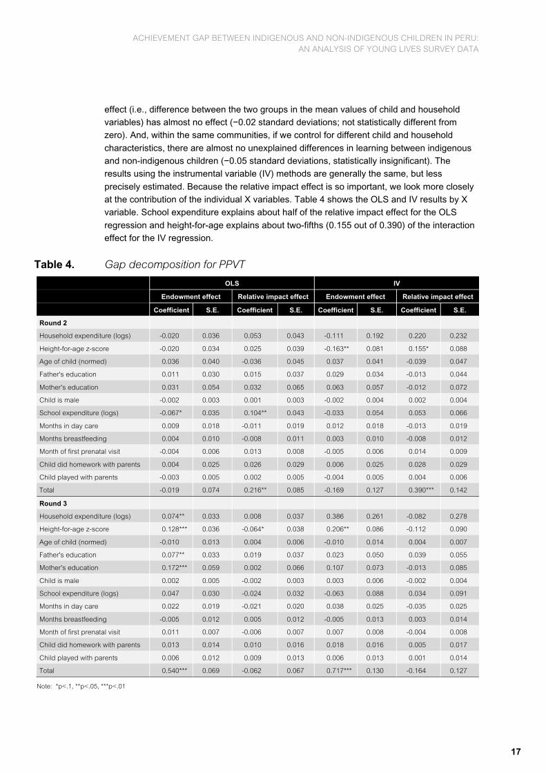
precisely estimated. Because the relative impact effect is so important, we look more closely at the contribution of the individual X variables. Table 4 shows the OLS and IV results by X variable. School expenditure explains about half of the relative impact effect for the OLS
regression and height-for-age explains about two-fifths (0.155 out of 0.390) of the interaction effect for the IV regression.
Table 4. Gap decomposition for PPVT
OLS IV
Endowment effect Relative impact effect Endowment effect Relative impact effect
Coefficient S.E. Coefficient S.E. Coefficient S.E. Coefficient S.E.
Round 2
Household expenditure (logs) -0.020 0.036 0.053 0.043 -0.111 0.192 0.220 0.232
Height-for-age z-score -0.020 0.034 0.025 0.039 -0.163** 0.081 0.155* 0.088
Age of child (normed) 0.036 0.040 -0.036 0.045 0.037 0.041 -0.039 0.047
Father's education 0.011 0.030 0.015 0.037 0.029 0.034 -0.013 0.044
Mother's education 0.031 0.054 0.032 0.065 0.063 0.057 -0.012 0.072
Child is male -0.002 0.003 0.001 0.003 -0.002 0.004 0.002 0.004
School expenditure (logs) -0.067* 0.035 0.104** 0.043 -0.033 0.054 0.053 0.066
Months in day care 0.009 0.018 -0.011 0.019 0.012 0.018 -0.013 0.019
Months breastfeeding 0.004 0.010 -0.008 0.011 0.003 0.010 -0.008 0.012
Month of first prenatal visit -0.004 0.006 0.013 0.008 -0.005 0.006 0.014 0.009
Child did homework with parents 0.004 0.025 0.026 0.029 0.006 0.025 0.028 0.029
Child played with parents -0.003 0.005 0.002 0.005 -0.004 0.005 0.004 0.006
Total -0.019 0.074 0.216** 0.085 -0.169 0.127 0.390*** 0.142
Round 3
Household expenditure (logs) 0.074** 0.033 0.008 0.037 0.386 0.261 -0.082 0.278
Height-for-age z-score 0.128*** 0.036 -0.064* 0.038 0.206** 0.086 -0.112 0.090
Age of child (normed) -0.010 0.013 0.004 0.006 -0.010 0.014 0.004 0.007
Father's education 0.077** 0.033 0.019 0.037 0.023 0.050 0.039 0.055
Mother's education 0.172*** 0.059 0.002 0.066 0.107 0.073 -0.013 0.085
Child is male 0.002 0.005 -0.002 0.003 0.003 0.006 -0.002 0.004
School expenditure (logs) 0.047 0.030 -0.024 0.032 -0.063 0.088 0.034 0.091
Months in day care 0.022 0.019 -0.021 0.020 0.038 0.025 -0.035 0.025
Months breastfeeding -0.005 0.012 0.005 0.012 -0.005 0.013 0.003 0.014
Month of first prenatal visit 0.011 0.007 -0.006 0.007 0.007 0.008 -0.004 0.008
Child did homework with parents 0.013 0.014 0.010 0.016 0.018 0.016 0.005 0.017
Child played with parents 0.006 0.012 0.009 0.013 0.006 0.013 0.001 0.014
Total 0.540*** 0.069 -0.062 0.067 0.717*** 0.130 -0.164 0.127
Note: *p<.1, **p<.05, ***p<.01

ACHIEVEMENT GAP BETWEEN INDIGENOUS AND NON-INDIGENOUS CHILDREN IN PERU: AN ANALYSIS OF YOUNG LIVES SURVEY DATA
18
In sum, these results attribute about one-half of the initial achievement gap in vocabulary to
the fact that indigenous children live in communities whose characteristics cause all children to have lower vocabulary skills; the rest of the gap is explained by differences between
indigenous and non-indigenous children in the impacts of child and household variables. It is also important to consider what the results do not show. The results do not reveal which community characteristics cause 5-year-old children to have better vocabularies in some
communities than in others. The results also do not show which child and household variables had differential impacts
The second set of results in Table 3 presents the decomposition of the CDA-Q (maths) test
scores in Round 2, when the children were 5 years old. Recall that the achievement gap here
was small (0.20 standard deviations), so there is little gap to explain. Indeed, the OLS results indicate that all four components of the conceptual model have statistically insignificant impacts. The IV results, while somewhat different, are also mostly statistically insignificant.
The Wu-Hausman test reveals no significant difference between the OLS and IV estimates. Overall, it is not possible to determine what factors explain the small gap found in maths test scores at the age of 5.
The remaining columns of Table 3 show the decompositions for Round 3, when the children
were about 8 years old and had been in primary school for nearly three years. Looking at the OLS estimates for the PPVT, the endowment effect, or differences in household and child characteristics, explains 80 per cent of the achievement gap. The community sorting effect
and the community impact effect also had significant impacts, but they offset each other. These scores offset each other because the distribution of indigenous children across the 19 communities is actually favourable; it reduces the gap by −0.19 standard deviations. This
means that, in contrast to the results for Round 2 vocabulary scores, indigenous children are more likely to live in communities where the community characteristics are favourable for learning maths skills, although this effect is significant only at the 10 per cent level. However,
the community impact effect suggests that this advantage is outweighed by the fact that within the same community indigenous children do not experience the community gain of αj
NI obtained by non-indigenous children. Instead, indigenous children’s community gain of αj
I is
on average lower than αjNI and therefore adds 0.38 standard deviations to the overall gap.10
This effect accounts for about for about half of the overall gap of 0.66. That is, indigenous children learn less in the same communities as non-indigenous children, even after
controlling for family and child characteristics. Finally, note that the IV analysis yielded similar results, although less precisely estimated.
Recall that for vocabulary scores when the children were 5 years old, the endowment effect
had virtually no impact. Yet, by 8 years old, the endowment effect explains 80 per cent of the achievement gap in vocabulary. Therefore, it is useful to see which X variables are most
important in explaining the endowment effect for Round 3 PPVT scores. Table 4 shows the OLS and IV results by X variable. Together, mothers’ and fathers’ education explain almost half of the endowment effect; about one-third (0.17 out of 0.54) is due to differences in
mothers’ education and almost one-sixth is due to differences in father’s education. Differences in child nutritional status explain another one-quarter, and the rest is mostly due to differences in household expenditure, including educational expenditure. Unfortunately,
10 Strictly speaking, these j
NI and jI terms refer to the community effects for the average indigenous student, that is a student for
whom XX = X, not a student for whom XX = 00.

ACHIEVEMENT GAP BETWEEN INDIGENOUS AND NON-INDIGENOUS CHILDREN IN PERU: AN ANALYSIS OF YOUNG LIVES SURVEY DATA
19
the IV results are again imprecisely estimated; the only statistically significant estimate is for child nutritional status, which again explains about one-quarter of the gap (0.21 out of 0.72).
Finally, we return to Table 3 to consider the OLS estimates of the decomposition of the
maths results for 2009, when the children were 8 years old. Here, the endowment effect
alone explains all of the achievement gap (0.51 out of 0.49). As was the case with vocabulary scores in this round, the community sorting effect and the community impact also had significant impacts, but they offset each other. The distribution of indigenous children across
those communities (community sorting effect) is favourable to indigenous children because it reduces the achievement gap by −0.22 standard deviations. But, this advantage is outweighed by the fact that, on average, indigenous children gain less from community (and
school) characteristics that contribute to learning maths than do non-indigenous children in the same community; in other words, αj
I is, on average, lower than αjNI. Again, the IV results
are broadly similar.
Because the endowment effect is so important here, we again look more closely at the
contribution of individual X variables. Table 5 shows the largest single factor is mothers’ education, which explains about one-third of the endowment effect (0.16 out of 0.51). The other two factors with large impacts are household expenditure on education and nutritional
status (height-for-age z-score), both of which explain about one-fifth of the endowment effect. The IV analysis was again less precisely estimated. There are only two statistically significant estimates, the larger of which is the impact of child nutrition, which explains about one-
quarter of the overall achievement gap. For the IV results, the relative impacts effect is marginally statistically significant, and the value of −0.257 indicates that the impacts of the X variables are somewhat stronger for indigenous students; the only significant variable is the
one indicating that the parent helped the child with homework, but it accounts for only one-sixth of the relative impact effect.
The differences in the structure of the test scores gaps between the age of 5 and the age of 8
requires further comment. At the age of 5, almost all of the differences are between communities, and it is difficult with the data at hand to understand the causes of those
differences. Yet by the age of 8 child and household characteristics play a major role. One possible reason for this change between the ages of 5 and 8 is that for most children the intensity of learning increases dramatically when they enter primary school, and it is only
then that differential advantage in terms of parental education, child nutrition, and other factors begin to play a large role. Indeed, some household variables, such as school expenditure and time spent doing homework with parents, are largely irrelevant to the
acquisition of skills before children start primary school.

ACHIEVEMENT GAP BETWEEN INDIGENOUS AND NON-INDIGENOUS CHILDREN IN PERU: AN ANALYSIS OF YOUNG LIVES SURVEY DATA
20
Table 5. Gap decomposition for maths
OLS IV
Endowment effect Relative impact effect Endowment effect Relative impact effect
Coefficient SE Coefficient SE Coefficient SE Coefficient SE
Round 2
Household expenditure (logs) 0.024 0.043 -0.026 0.052 -0.324 0.262 0.440 0.305
Height-for-age z-score 0.002 0.042 -0.001 0.047 -0.051 0.103 0.105 0.111
Age of child (normed) 0.014 0.049 -0.031 0.055 0.026 0.052 -0.047 0.058
Father's education 0.035 0.037 -0.019 0.044 0.067 0.044 -0.071 0.055
Mother's education 0.022 0.066 0.047 0.079 0.058 0.073 -0.031 0.089
Child is male -0.001 0.003 0.001 0.002 -0.001 0.003 0.001 0.003
School expenditure (logs) -0.109 0.043 0.115** 0.051 -0.026 0.071 -0.007 0.085
Months in day care 0.015 0.021 -0.018 0.022 0.021 0.023 -0.023 0.024
Months breastfeeding -0.002 0.010 -0.007 0.012 -0.001 0.011 -0.009 0.013
Month of first prenatal visit 0.000 0.006 0.011 0.009 -0.001 0.007 0.011 0.009
Child did homework with parents 0.016 0.031 -0.011 0.035 0.011 0.033 -0.003 0.037
Child played with parents 0.000 0.005 0.000 0.006 -0.004 0.006 0.004 0.007
Total 0.016 0.090 0.060 0.102 -0.225 0.175 0.371* 0.190
Round 3
Household expenditure (logs) 0.039 0.032 0.002 0.037 0.383 0.283 -0.167 0.303
Height-for-age z-score 0.096*** 0.036 -0.022 0.039 0.192** 0.088 -0.110 0.094
Age of child (normed) -0.008 0.016 0.001 0.003 -0.008 0.016 0.002 0.004
Father's education 0.028 0.032 0.058 0.038 -0.031 0.050 0.091 0.057
Mother's education 0.162 0.057 -0.002 0.067 0.096 0.072 0.005 0.087
Child is male 0.002*** 0.005 -0.001 0.003 0.002 0.006 -0.001 0.003
School expenditure (logs) 0.098*** 0.030 -0.046 0.031 -0.022 0.092 0.035 0.095
Months in day care 0.010 0.018 -0.011 0.019 0.029 0.025 -0.029 0.026
Months breastfeeding 0.010 0.011 -0.011 0.012 0.010 0.012 -0.012 0.013
Month of first prenatal visit 0.004 0.006 -0.005 0.007 0.001 0.006 -0.003 0.007
Child did homework with parents 0.053*** 0.017 -0.038** 0.017 0.060*** 0.019 -0.045** 0.020
Child played with parents 0.017 0.013 -0.016 0.014 0.018 0.014 -0.024 0.017
Total 0.511*** 0.069 -0.089 0.069 0.731*** 0.146 -0.257* 0.145
Note: *p<.1, **p<.05, ***p<.01

ACHIEVEMENT GAP BETWEEN INDIGENOUS AND NON-INDIGENOUS CHILDREN IN PERU: AN ANALYSIS OF YOUNG LIVES SURVEY DATA
21
8. Conclusion and policy implications This study has used recent household panel data to attempt to explain the large and persistent achievement gap that exists between indigenous and non-indigenous children in
Peru. The new information our analysis provides is dramatic. Through our analysis we learn that at the age of 5, almost all of the differences between indigenous and non-indigenous children’s achievement are due to the communities they live in, not to child or household
characteristics. Yet by the age of 8, the importance of community characteristics recedes and household and child characteristics clearly play the major role. Differences in household and child characteristics account for 80 per cent of the gap in the PPVT scores at the age of 8
and virtually all the gap in CDA-Q test scores. One possible reason for this change between the ages of 5 and 8 is that for most children, the intensity of learning increases dramatically when they enter primary school. When this happens, differences in parental education, child
nutrition and other factors become more relevant.
Given that household and child characteristics account for so much of the achievement gap,
what are the most important underlying causes? In short, the main cause is parental education. Nearly half the vocabulary endowment effect is due to differences in parental
education; one-third from mothers’ education and almost one-sixth from fathers’ education. Similarly, for maths, mothers’ education explains about one-third of the achievement gap. For vocabulary, differences in children’s nutritional status explain another quarter of the gap, and
the rest is mostly due to differences in household expenditure, including educational expenditure. For maths, the other two X variables with large impacts are children’s nutritional status and expenditure on schooling, both of which explain about one-fifth of the
achievement gap.
Similar to previous findings in developing countries (Alderman et al. 2001; Glewwe et al.
2001; Glewwe and Miguel 2008 ), we find that children’s nutritional experiences in the first years of life affect their subsequent acquisition of skills. This suggests that policymakers
should focus their efforts on nutritional programmes that target children in the first years of their lives.
In addition to that, these results point clearly and convincingly in a specific policy direction:
increasing indigenous children’s years of education. Because today’s indigenous children will be tomorrow’s indigenous parents, and because our analysis shows that the number of years
they attend school will have the single biggest, most positive effect on their own children’s educational achievement, Peru should pursue policies that will increase the years of schooling that indigenous children attain. However, in the light of the fact that school
enrolment does not always mean school attendance, much less learning, particularly for indigenous children, policymakers need research that specifies which strategies are most effective for increasing years of completed schooling and increasing the learning that takes
place during those years, among Peru’s indigenous population.

ACHIEVEMENT GAP BETWEEN INDIGENOUS AND NON-INDIGENOUS CHILDREN IN PERU: AN ANALYSIS OF YOUNG LIVES SURVEY DATA
22
References Alderman, H., J.R. Behrman, V. Lavy and R. Menon (2001) ‘Child Health and School
Enrolment: A Longitudinal Analysis’, The Journal of Human Resources 36.1: 185–205.
Becker, G.S. (1965) ‘A Theory of the Allocation of Time’, The Economic Journal 75.299: 493–
517.
Becketti, S., W. Gould, L. Lillard and F. Welch (1988) ‘The Panel Study of Income Dynamics
After Fourteen Years: An Evaluation’, Journal of Labor Economics 6.4: 472–92.
Bernal, R. (2008) ‘The Effect of Maternal Employment and Child Care on Children’s
Cognitive Development’, International Economic Review 49.4: 1173–209.
Blinder, A.S. (1973) ‘Wage Discrimination: Reduced Form and Structural Estimates’, Journal
of Human Resources 8.4: 436–55.
Bradley, S., M. Draca, C. Green and G. Leeves (2007) ‘The Magnitude of Educational
Disadvantage of Indigenous Minority Groups in Australia’, Journal of Population Economics
20.3: 547–69.
Castillo, M.Z., N. Bariola and T. Ponce (2008) La educación intercultural bilingüe: El caso
peruano, Lima: Foro Educativo.
Cook, M.D. and W.N. Evans (2000) ‘Families or Schools? Explaining the Convergence in
White and Black Academic Performance’, Journal of Labor Economics 18.4: 729–54.
Currie, J. (2009) ‘Healthy, Wealthy, and Wise: Socioeconomic Status, Poor Health in
Childhood, and Human Capital Development’, Journal of Economic Literature 47.1: 87–122.
Driessen, G., F. Smit and P. Sleegers (2005) ‘Parental Involvement and Educational
Achievement’, British Educational Research Journal 31.4: 509–32.
Fishel, M. and L. Ramirez (2005) ‘Evidence-Based Parent Involvement Interventions with
School-Aged Children’, School Psychology Quarterly 20.4: 371–402.
Fortin, N., T. Lemieux and S. Firpo (2011) ‘Decomposition Methods in Economics’ in O.
Ashenfelter and D. Card (eds) Handbook of Labor Economics, Volume 4A, Amsterdam: North-Holland.
Glewwe, P. and E.A. Miguel (2008) ‘The Impact of Child Health and Nutrition on Education in
Less Developed Countries’ in T. Paul Schultz and John Strauss (eds) Handbook of
Development Economics, Volume 4:, Amsterdam: North Holland.
Glewwe, P., S. Krutikova and C. Rolleston (2013) ‘Decomposing Student Learning Gaps in
Developing Countries: Evidence from Peruvian and Vietnamese Data’, presentation given at the conference ‘Inequalities in Children’s Outcomes in Developing Countries’, University of
Oxford, 8–9 July 2013, http://www.younglives.org.uk/files/others/inequalities-conference-plenary-presentations/paul-glewwe.
Glewwe, P., H. Jacoby and E.M. King (2001) ‘Early Childhood Nutrition and Academic
Achievement: A Longitudinal Analysis’, Journal of Public Economics 81.3: 345–68.
Hernandez-Zavala, M., H.A. Patrinos, C. Sakellariou and J. Shapiro (2006) Quality of
Schooling and Quality of Schools for Indigenous Students in Guatemala, Mexico and Peru,
Working Paper 3982, Washington, DC: World Bank.
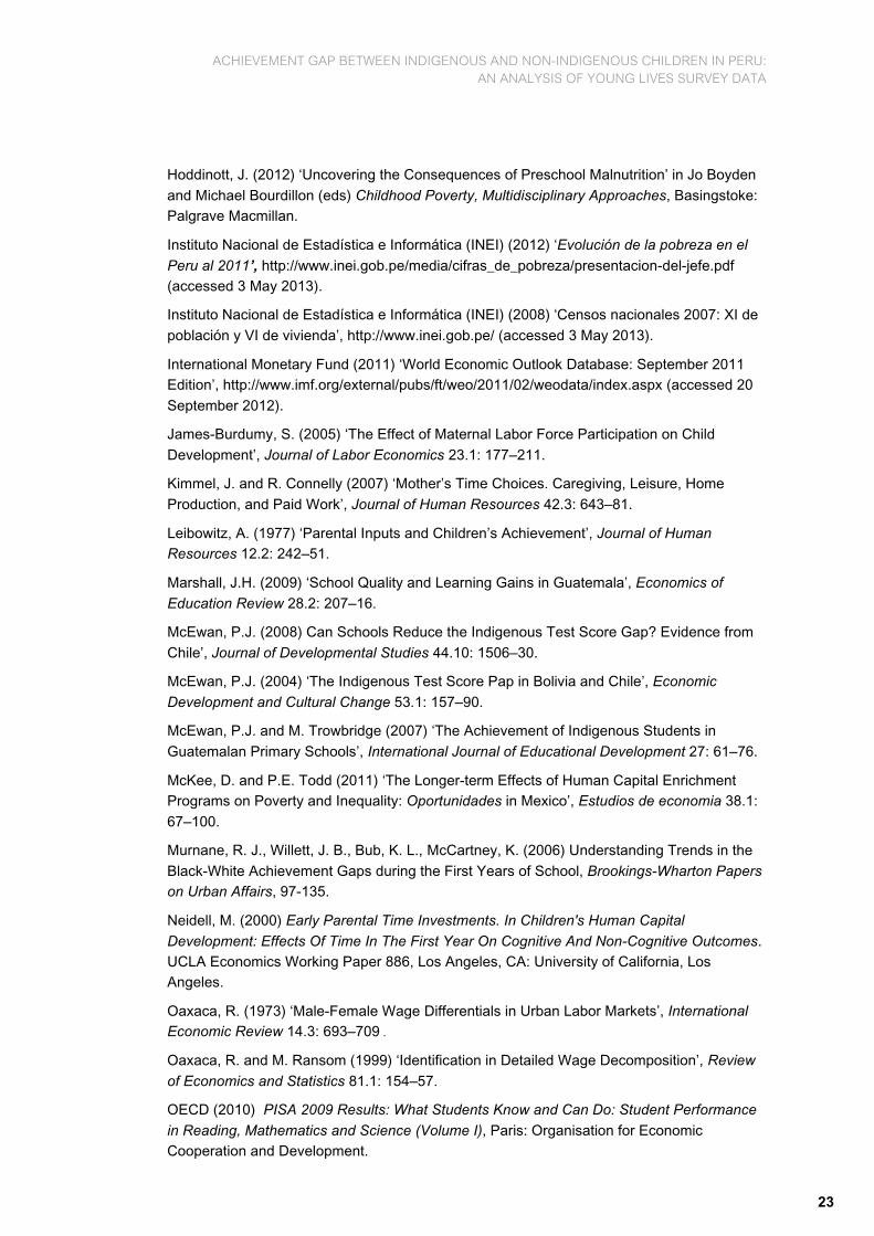
ACHIEVEMENT GAP BETWEEN INDIGENOUS AND NON-INDIGENOUS CHILDREN IN PERU: AN ANALYSIS OF YOUNG LIVES SURVEY DATA
23
Hoddinott, J. (2012) ‘Uncovering the Consequences of Preschool Malnutrition’ in Jo Boyden
and Michael Bourdillon (eds) Childhood Poverty, Multidisciplinary Approaches, Basingstoke: Palgrave Macmillan.
Instituto Nacional de Estadística e Informática (INEI) (2012) ‘Evolución de la pobreza en el
Peru al 2011’, http://www.inei.gob.pe/media/cifras_de_pobreza/presentacion-del-jefe.pdf (accessed 3 May 2013).
Instituto Nacional de Estadística e Informática (INEI) (2008) ‘Censos nacionales 2007: XI de
población y VI de vivienda’, http://www.inei.gob.pe/ (accessed 3 May 2013).
International Monetary Fund (2011) ‘World Economic Outlook Database: September 2011 Edition’, http://www.imf.org/external/pubs/ft/weo/2011/02/weodata/index.aspx (accessed 20
September 2012).
James-Burdumy, S. (2005) ‘The Effect of Maternal Labor Force Participation on Child
Development’, Journal of Labor Economics 23.1: 177–211.
Kimmel, J. and R. Connelly (2007) ‘Mother’s Time Choices. Caregiving, Leisure, Home
Production, and Paid Work’, Journal of Human Resources 42.3: 643–81.
Leibowitz, A. (1977) ‘Parental Inputs and Children’s Achievement’, Journal of Human Resources 12.2: 242–51.
Marshall, J.H. (2009) ‘School Quality and Learning Gains in Guatemala’, Economics of
Education Review 28.2: 207–16.
McEwan, P.J. (2008) Can Schools Reduce the Indigenous Test Score Gap? Evidence from
Chile’, Journal of Developmental Studies 44.10: 1506–30.
McEwan, P.J. (2004) ‘The Indigenous Test Score Pap in Bolivia and Chile’, Economic
Development and Cultural Change 53.1: 157–90.
McEwan, P.J. and M. Trowbridge (2007) ‘The Achievement of Indigenous Students in
Guatemalan Primary Schools’, International Journal of Educational Development 27: 61–76.
McKee, D. and P.E. Todd (2011) ‘The Longer-term Effects of Human Capital Enrichment Programs on Poverty and Inequality: Oportunidades in Mexico’, Estudios de economia 38.1:
67–100.
Murnane, R. J., Willett, J. B., Bub, K. L., McCartney, K. (2006) Understanding Trends in the
Black-White Achievement Gaps during the First Years of School, Brookings-Wharton Papers on Urban Affairs, 97-135.
Neidell, M. (2000) Early Parental Time Investments. In Children's Human Capital
Development: Effects Of Time In The First Year On Cognitive And Non-Cognitive Outcomes. UCLA Economics Working Paper 886, Los Angeles, CA: University of California, Los Angeles.
Oaxaca, R. (1973) ‘Male-Female Wage Differentials in Urban Labor Markets’, International Economic Review 14.3: 693–709 .
Oaxaca, R. and M. Ransom (1999) ‘Identification in Detailed Wage Decomposition’, Review
of Economics and Statistics 81.1: 154–57.
OECD (2010) PISA 2009 Results: What Students Know and Can Do: Student Performance
in Reading, Mathematics and Science (Volume I), Paris: Organisation for Economic Cooperation and Development.

ACHIEVEMENT GAP BETWEEN INDIGENOUS AND NON-INDIGENOUS CHILDREN IN PERU: AN ANALYSIS OF YOUNG LIVES SURVEY DATA
24
Outes-Leon, I. and S. Dercon (2008) Survey Attrition and Attrition Bias in Young Lives,
Technical Note 5, Oxford: Young Lives.
Paxson, C. and N. Schady (2007) ‘Cognitive Development Among Young Children in
Ecuador: The Role of Health, Wealth and Parenting’, Journal of Human Resources 42.1: 49–
84.
Pitt, M., M. Rosenzweig and D. Gibbons (1993) ‘The Determinants and Consequences of the
Placement of Government Programs in Indonesia’, World Bank Economic Review 7.3: 319–48.
Rosenzweig, M. and K. Wolpin (1994) ‘Are There Increasing Returns to the Intergenerational Production of Human Capital? Maternal Schooling and Child Intellectual Achievement’,
Journal of Human Resources 29.2: 670–93.
Sakellariou, C. (2008) ‘Peer Effects and the Indigenous/Non‐indigenous Early Test‐Score
Gap in Peru’, Education Economics 16.4: 371–90.
Schady, N. (2006) Early Childhood Development in Latin America and the Caribbean, Policy
Research Working Paper 3869, Washington, DC: World Bank.
Shin, H. (2007) ‘Child Health in Peru: Importance of Regional Variation and Community Effects on Children's Height and Weight’, Journal of Health and Social Behavior 48.4: 418–
33.
Stein, Z., M. Susser, G. Saenger and F. Marolla (1975) Famine and Human Development:
The Dutch Hunger Winter of 1944-45, New York: Oxford University Press.
Solis-Fonseca, G. (2009) ‘Perú Amazónico’ in Atlas sociolinguuístico de pueblos indígenas
en América Latina, Cochabamba, Bolivia: UNICEF and FUNPROEIB Andes .
Stock J, and M. Yogo (2005) ‘Testing for Weak Instruments in Linear IV Regression’ in
Donald W.K. Andrews and James H. Stock (eds) Identification and Inference for Econometric
Models: Essays in Honor of Thomas J. Rothenberg, New York: Cambridge University Press.
Todd, P. and K. Wolpin (2007) ‘The Production of Cognitive Achievement in Children: Home,
School, and Racial Test Scores Gaps’, Journal of Human Capital 1.1: 91–136.
Umbel, V.M., B.Z. Pearson, M.C. Fernandez and D.K. Oller (1992) ‘Measuring Bilingual
Children’s Receptive Vocabularies’, Child Development 63.4: 1012–20.
UNICEF (2009) The State of the World’s Children Special Edition: Celebrating 20 Years of
the Convention on the Rights of the Child, New York: UNICEF.
United Nations (2010) Human Development Report 2010. The Real Wealth of Nations:
Pathways to Human Development, New York: Palgrave Macmillan.
Vásquez-Huamán, E., A. Chumpitaz and C. Jara (2008) Niñez Indígena y Educación
Intercultural Bilingüe en el Perú: Estadísticas recientes, preguntas (i) resueltas y tareas pendientes, Lima: Asociación Grafica Educativa Tarea.
Villar, J., V. Smerglio, R. Martorell, C.H. Brown and R.E. Klein (1984) ‘Heterogenous Growth
and Mental Development of Intrauterine Growth-retarded Infants During the First 3 Years of
Life’, Pediatrics 74.5: 783–91.
Waber, D., L. Vuori-Christiansen, N. Ortiz, J. Clement, N. Christiansen, J. Mora, R. Reed and
G. Herrera (1981) ‘Nutritional Supplementation, Maternal Education, and Cognitive

ACHIEVEMENT GAP BETWEEN INDIGENOUS AND NON-INDIGENOUS CHILDREN IN PERU: AN ANALYSIS OF YOUNG LIVES SURVEY DATA
25
Development of Infants at Risk of Malnutrition’, American Journal of Clinical Nutrition 34: 807–13.
Wilcox-Gök, V. (1983) ‘The Determination of Child Health: An Application of Sibling and
Adoption Data’, Review of Economics and Statistics 65.5: 266–73.
Wooldridge, J. (2010) Econometric Analysis of Cross-section and Panel Data, 2nd edn,
Cambridge, MA: MIT Press.
World Bank (2011) ‘Data. Latin America and Caribbean (Developing Only)’,
http://data.worldbank.org/region/LAC?display=default (accessed 1 April 2013).
World Bank (2010) ‘Poverty and Equity. Country Dashboard: Peru’,
http://povertydata.worldbank.org/poverty/country/PER (accessed 1 April 2013).
World Bank (2001) World Development Report 2000/2001: Attacking Poverty, Washington,
DC: World Bank.

ACHIEVEMENT GAP BETWEEN INDIGENOUS AND NON-INDIGENOUS CHILDREN IN PERU: AN ANALYSIS OF YOUNG LIVES SURVEY DATA
26
Appendix
Table A1. First-stage regressions
Non-indigenous Indigenous
HH exp. (logs) HAZ HH exp. (logs) HAZ
Coef. SE Coef. SE Coef. SE Coef. SE
PPVT
Age of child (normed) 0.006 0.007 0.029*** 0.010 0.004 0.016 -0.013 0.019
Father's education 0.018*** 0.006 0.006 0.008 0.022** 0.009 0.024** 0.011
Mother's education 0.024*** 0.006 0.025*** 0.008 0.011 0.010 0.023** 0.011
Child is male -0.016 0.031 0.041 0.042 -0.032 0.059 0.051 0.069
School expenditure (logs) 0.190*** 0.016 0.127*** 0.023 0.304*** 0.038 0.099** 0.045
Months in day care -0.002 0.002 0.004 0.003 -0.012 0.008 -0.009 0.009
Months breastfeeding -0.004 0.007 0.019* 0.010 -0.006 0.016 0.042** 0.019
Month of first prenatal visit 0.000 0.008 -0.023** 0.012 -0.014 0.015 -0.004 0.017
Child did homework with parents -0.001 0.015 -0.015 0.021 -0.018 0.024 -0.013 0.028
Child played with parents 0.045*** 0.011 -0.006 0.015 -0.001 0.021 -0.032 0.024
Wealth index (Round 1) 0.749*** 0.113 0.338** 0.156 0.670*** 0.231 0.668** 0.270
HAZ (Round 1) 0.033** 0.014 0.478*** 0.019 -0.002 0.026 0.310*** 0.030
Maths
Age of child (normed) 0.006 0.007 0.031*** 0.010 0.003 0.017 -0.013 0.019
Father's education 0.017*** 0.006 0.005 0.008 0.021** 0.010 0.025** 0.011
Mother's education 0.024*** 0.006 0.024*** 0.008 0.009 0.010 0.020* 0.011
Child is male -0.012 0.031 0.042 0.042 -0.023 0.060 0.059 0.070
School expenditure (logs) 0.188*** 0.016 0.131*** 0.022 0.302*** 0.039 0.107** 0.045
Months in day care -0.002 0.002 0.004 0.003 -0.014* 0.008 -0.009 0.009
Months breastfeeding -0.004 0.007 0.014 0.010 -0.004 0.016 0.041** 0.019
Month of first prenatal visit -0.002 0.009 -0.024** 0.012 -0.010 0.015 -0.008 0.017
Child did homework with parents 0.002 0.015 -0.016 0.021 -0.022 0.024 -0.017 0.029
Child played with parents 0.047*** 0.011 -0.006 0.015 -0.001 0.021 -0.028 0.024
Wealth index (Round 1) 0.753*** 0.114 0.382** 0.154 0.628*** 0.234 0.638** 0.274
HAZ (Round 1) 0.031** 0.014 0.479*** 0.019 0.003 0.026 0.313*** 0.030
Notes: Each column corresponds to a different regression. Each regression controls for district dummies.
HH exp. (logs)= household expenditure in logs; HAZ= height-for-age z-score.
*p<.1, **p<.05, ***p<.01

ACHIEVEMENT GAP BETWEEN INDIGENOUS AND NON-INDIGENOUS CHILDREN IN PERU: AN ANALYSIS OF YOUNG LIVES SURVEY DATA
27
Table A2 Panel A – Estimated coefficients for PPVT, second stage ROUND 2 ROUND 3
Non-indigenous Indigenous Non-indigenous Indigenous
OLS IV OLS IV OLS IV OLS IV
Coeff SE Coeff SE Coeff SE Coeff SE Coeff SE Coeff SE Coeff SE Coeff SE
Household expenditure (logs)
0.056 0.042 0.188 0.224 -0.035 0.062 -0.191 0.331 0.175*** 0.037 0.650*** 0.215 0.158** 0.069 0.827 0.554
Height-for-age z-score 0.007 0.025 -0.012 0.047 -0.028 0.048 -0.227** 0.111 0.097*** 0.022 0.142*** 0.045 0.194*** 0.053 0.311** 0.127
Age of child (normed) 0.000 0.010 -0.001 0.010 0.017 0.019 0.018 0.020 0.038*** 0.009 0.036*** 0.010 0.062*** 0.023 0.064** 0.026
Father's education 0.011 0.009 0.007 0.011 0.005 0.013 0.012 0.014 0.040*** 0.007 0.026*** 0.010 0.032** 0.013 0.009 0.021
Mother's education 0.015* 0.008 0.012 0.010 0.007 0.013 0.015 0.013 0.041*** 0.007 0.022** 0.010 0.040*** 0.014 0.025 0.017
Child is male -0.021 0.046 -0.017 0.046 -0.110 0.079 -0.148* 0.081 0.051 0.040 0.061 0.042 0.166** 0.083 0.198** 0.093
School expenditure (logs) 0.026 0.017 0.014 0.027 -0.046* 0.024 -0.023 0.037 0.046** 0.022 -0.058 0.047 0.093 0.059 -0.125 0.174
Months in day care -0.001 0.004 -0.001 0.004 0.005 0.010 0.007 0.011 0.001 0.003 0.002 0.003 0.013 0.011 0.022 0.014
Months breastfeeding 0.009 0.010 0.011 0.010 -0.008 0.020 -0.006 0.020 0.001 0.009 0.003 0.010 0.010 0.023 0.010 0.026
Month of first prenatal visit -0.031** 0.013 -0.031** 0.013 0.014 0.019 0.018 0.020 -0.016 0.011 -0.012 0.012 -0.037* 0.021 -0.025 0.024
Child did homework with parents
0.115** 0.054 0.126** 0.057 0.016 0.095 0.021 0.095 0.059*** 0.020 0.059*** 0.021 0.034 0.035 0.047 0.039
Child played with parents -0.018 0.064 -0.011 0.064 -0.071 0.122 -0.124 0.131 0.040*** 0.014 0.018 0.018 0.016 0.029 0.016 0.032
Test of endogeneity
Durbin score (chi-square) 0.408 5.520 14.623 4.676
p-value 0.816 0.063 0.001 0.097
Wu-Hausman test 0.198 2.629 7.199 2.222
p-value 0.820 0.073 0.001 0.110
Test for weak instruments
Stock & Yogo (2005) gmin=
9.224 13.3456 5.027 3.912
Notes: *p<.1, **p<.05, ***p<.01
Stock and Yogo (2005) state that instruments are weak if the conventional 5%- level Wald test based on IV statistics has an actual size that could exceed a certain threshold r. The critical values when we have two instruments and two endogenous regressors are 7.03 (r=10%), 4.58 (r=15%), 3.95 (r=20%) and 3.63 (r=25%). The null hypothesis is that the instruments are weak. We reject the null hypothesis if gmin (minimum eigenvalue statistic) >critical value.
Table A2 Panel B – Estimated coefficients for maths, second stage Round 2 ROUND 3
Non-indigenous Indigenous Non-indigenous Indigenous
OLS IV OLS IV OLS IV OLS IV
Coeff SE Coeff SE Coeff SE Coeff SE Coeff SE Coeff E Coeff SE Coeff SE
Household expenditure (logs)
-0.002 0.049 0.192 0.234 0.043 0.075 -0.190 0.355 0.089** 0.043 0.466* 0.240 0.084 0.068 0.826 0.605
Height-for-age z-score 0.002 0.029 -0.017 0.049 0.002 0.059 -0.226** 0.112 0.110*** 0.026 0.123** 0.050 0.143*** 0.052 0.286** 0.129
Age of child (normed) -0.008 0.012 0.000 0.010 0.007 0.023 0.015 0.020 0.065*** 0.011 0.063*** 0.011 0.075*** 0.023 0.079*** 0.026
Father's education 0.007 0.010 0.008 0.012 0.015 0.015 0.009 0.014 0.036*** 0.009 0.025** 0.011 0.012 0.013 -0.013 0.021
Mother's education 0.016 0.010 0.012 0.010 0.005 0.016 0.015 0.013 0.038*** 0.008 0.024** 0.011 0.038*** 0.013 0.022 0.017
Child is male -0.019 0.054 -0.027 0.047 -0.085 0.096 -0.140* 0.081 0.087* 0.046 0.093** 0.048 0.173** 0.082 0.201** 0.092
School expenditure (logs) 0.004 0.019 0.012 0.027 -0.076*** 0.029 -0.021 0.038 0.106*** 0.026 0.028 0.052 0.200*** 0.058 -0.044 0.188
Months in day care -0.002 0.004 -0.001 0.004 0.009 0.013 0.004 0.010 -0.001 0.004 0.000 0.004 0.006 0.011 0.018 0.015
Months breastfeeding 0.022* 0.012 0.009 0.011 0.004 0.024 -0.001 0.020 0.002 0.011 0.004 0.011 -0.023 0.023 -0.024 0.026
Month of first prenatal visit -0.042*** 0.015 -0.029** 0.013 0.000 0.024 0.024 0.020 0.004 0.013 0.007 0.013 -0.014 0.020 -0.003 0.024
Child did homework with parents
0.017 0.063 0.126** 0.058 0.060 0.115 0.028 0.095 0.041* 0.023 0.040* 0.023 0.139*** 0.034 0.157*** 0.040
Child played with parents -0.008 0.075 -0.009 0.066 -0.003 0.149 -0.123 0.133 0.004 0.016 -0.015 0.020 0.041 0.029 0.042 0.032
Test of endogeneity
Durbin score (chi-square) 0.372 5.248 4.612 6.443
p-value 0.830 0.073 0.100 0.040
Wu-Hausman test 0.181 2.497 2.251 3.073
p-value 0.834 0.084 0.106 0.047
Test for weak instruments
Stock & Yogo (2005) gmin=
9.224 13.3456 4.734 3.419
Note: We use Table 2 in Stock and Yogo (2005) for critical values for the weak instrument test based on TSLS size at a significance level of 5%. The critical values when we have two instruments and two endogenous regressors are 7.03 (r=10%), 4.58 (r=15%), 3.95 (r=20%) and 3.63 (r=25%). The null hypothesis is that the instruments are weak. We reject the null hypothesis if gmin>critical value.
*p<.1, **p<.05, ***p<.01

ACHIEVEMENT GAP BETWEEN INDIGENOUS AND NON-INDIGENOUS CHILDREN IN PERU: AN ANALYSIS OF YOUNG LIVES SURVEY DATA
28
Table A3. Descriptive statistics for overall and restricted sample
Variable Our study Overall Diff-in-diff
Non-indigenous
(n.=1,210)
Indigenous
(n.=438)
Difference Non-indigenous Indigenous Difference (A-B) t-stat
(A) N. Mean N. Mean (B)
Household
expenditure, Round 2
9,792.837 5,909.292 3883.545*** 1,351 9680.264 509 5944.81 3,735.452*** 148.093 0.534
(8,621.119) (6,358.943) (229.820) (286.296)
Height-for-age z-
score, Round 2
-1.218 -1.937 0.719*** 1,346 -1.253 502 -1.952 0.698*** 0.021 0.554
(1.071) (0.922) (0.030) (0.043)
Age of child (normed),
Round 2
64.18 62.098 2.082*** 1,351 64.177 509 62.118 2.059*** 0.023 0.145
(4.572) (4.654) (0.126) (0.206)
Father’s education 9.969 7.564 2.405*** 1,287 9.961 466 7.494 2.468*** -0.063 -0.463
(3.713) (4.009) (0.104) (0.184)
Mother’s education 9.375 5.115 4.260*** 1,344 9.307 508 5.062 4.245*** 0.015 0.100
(3.872) (4.027) (0.107) (0.179)
Child is male 0.504 0.489 0.015 1,402 0.503 545 0.486 0.017 -0.002 -0.096
(0.500) (0.500) (0.013) (0.021)
School expenditure
(logs) Round 2
296.545 94.447 202.098*** 1,351 291.510 509 96.513 194.996*** 7.102 0.499
(472.253) (176.270) (12.667) (8.203)
Months in day care 2.752 1.041 1.711*** 1,402 2.578 545 1.013 1.566* 0.145 0.695
(6.933) (3.975) (0.180) (0.172)
Months breastfeeding 10.798 11.288 -0.490** 1,371 10.805 541 11.290 -0.485*** -0.005 -0.041
(3.681) (3.576) (0.099) (0.152)
Month of first prenatal
visit
2.944 3.237 -0.293*** 1,398 2.890 535 3.226 -0.336** 0.043 0.666
(1.875) (2.042) (0.051) (0.091)
Child did homework
with parents, Round 2
0.615 0.352 0.263*** 1,351 0.600 509 0.330 0.270*** -0.007 -0.429
(0.487) (0.478) (0.013) (0.021)
Child played with
parents, Round 2
0.157 0.121 0.036* 1,351 0.153 509 0.124 0.029 0.007 0.548
(0.364) (0.327) (0.010) (0.015)
Note: *p<.1, **p<.05, ***p<.01. Standard deviations are in parentheses. This table covers the 19 communities used in the analysis.


Achievement Gap between Indigenous and Non-Indigenous Children in Peru: An Analysis of Young Lives Survey Data
In Peru, indigenous children obtain lower scores on academic tests, on average, than non-indigenous children. In this study, we investigate whether a test score achievement gap is found by the age of 5 and whether this gap increases by the age of 8. While the literature has focused on the underlying family and children determinants of achievement gaps, we use an extension of the Oaxaca-Blinder technique to include community sorting effects and heterogeneity in community impact effects. Using the 2001 cohort of the Young Lives longitudinal survey for Peru, our results show that at the age of 5, indigenous children are far behind their non-indigenous counterparts in Spanish vocabulary (as measured by the PPVT), but less far behind in maths. Over the first three years of school, however, indigenous children lose substantial ground relative to non-indigenous children, increasing the average gap to 0.49 standard deviations (of the distribution of test scores) in maths and 0.66 in vocabulary. Our results suggest not only that parental education and a child’s health are important determinants of the gap for maths and vocabulary, as previously found in the literature; but also that the vocabulary gap is due in part to community effects. The pathways considered yield valuable information for policymakers who are interested in developing policies to improve student learning among indigenous groups. These pathways are important for human capital formation and could potentially have long-term impacts on educational attainment and poverty in Peru.
www.younglives.org.uk
About Young Lives
Young Lives is an international study of childhood poverty, involving 12,000 children in 4 countries over 15 years. It is led by a team in the Department of International Development at the University of Oxford in association with research and policy partners in the 4 study countries: Ethiopia, India, Peru and Vietnam.
Through researching different aspects of children’s lives, we seek to improve policies and programmes for children.
Young Lives Partners
Young Lives is coordinated by a small team based at the University of Oxford, led by Professor Jo Boyden.
• EthiopianDevelopmentResearchInstitute,Ethiopia
• PankhurstDevelopmentResearchandConsultingplc
• SavetheChildren(Ethiopiaprogramme)
• CentreforEconomicandSocialSciences,AndhraPradesh,India
• SavetheChildrenIndia
• SriPadmavathiMahilaVisvavidyalayam(Women’sUniversity),AndhraPradesh,India
• GrupodeAnálisisparaelDesarollo(GRADE),Peru
• InstitutodeInvestigaciónNutricional,Peru
• CentreforAnalysisandForecasting,VietnameseAcademyof SocialSciences,Vietnam
• GeneralStatisticsOffice,Vietnam
• Universityof Oxford,UK
Contact:Young LivesOxford Department of International Development,University of Oxford,3 Mansfield Road,Oxford OX1 3TB, UKTel: +44 (0)1865 281751Email: [email protected]: www.younglives.org.uk