achieving energy-synchronized communication …zt/papers/achievingenergy...68 achieving...

68

Achieving Energy-Synchronized Communicationin Energy-Harvesting Wireless Sensor Networks

YU GU and LIANG HE, Singapore University of Technology and DesignTING ZHU, State University of New YorkTIAN HE, University of Minnesota

With advances in energy-harvesting techniques, it is now feasible to build sustainable sensor networksto support long-term applications. Unlike battery-powered sensor networks, the objective of sustainablesensor networks is to effectively utilize a continuous stream of ambient energy. Instead of pushing thelimits of energy conservation, we aim to design energy-synchronized schemes that keep energy suppliesand demands in balance. Specifically, this work presents Energy-Synchronized Communication (ESC) as atransparent middleware between the network layer and MAC layer that controls the amount and timing ofRF activity at receiving nodes. In this work, we first derive a delay model for cross-traffic at individual nodes,which reveals an interesting stair effect. This effect allows us to design a localized energy synchronizationcontrol with O(d3) time complexity that shuffles or adjusts the working schedule of a node to optimize cross-traffic delays in the presence of changing duty cycle budgets, where d is the node degree in the network. Underdifferent rates of energy fluctuations, shuffle-based and adjustment-based methods have different influenceson logical connectivity and cross-traffic delay, due to the inconsistent views of working schedules amongneighboring nodes before schedule updates. We study the trade-off between them and propose methods forupdating working schedules efficiently. To evaluate our work, ESC is implemented on MicaZ nodes withtwo state-of-the-art routing protocols. Both testbed experiment and large-scale simulation results showsignificant performance improvements over randomized synchronization controls.

Categories and Subject Descriptors: C.2.2 [Computer-Communication Networks]: Network Protocols

General Terms: Design, Algorithms, Performance

Additional Key Words and Phrases: Wireless sensor networks, low-duty-cycle networks, energy-synchronizedcommunication, logical connectivity

ACM Reference Format:Yu Gu, Liang He, Ting Zhu, and Tian He. 2014. Achieving energy-synchronized communication in energy-harvesting wireless sensor networks. ACM Trans. Embedd. Comput. Syst. 13, 2s, Article 68 (January 2014),26 pages.DOI: http://dx.doi.org/10.1145/2544375.2544388

1. INTRODUCTION

With the increasing need for cyber-physical interaction, wireless sensor networks(WSN) have emerged as a key technology for many long-term applications, such as

Some preliminary results of this article [Gu et al. 2009b] appeared in Proceedings of the 17th IEEE Interna-tional Conference on Network Protocols (ICNP’09).This work was supported in part by the Singapore-MIT International Design Center IDG31000101, GrantSUTD SRG ISTD 2010 002, SUTD-ZJU/RES/03/2011, and NSF grant CNS-1217791.Authors’ addresses: Y. Gu (corresponding author) and L. He, Singapore University of Technology and Design,Singapore; T. Zhu, State University of New York, Binghamton; T. He, University of Minnesota, Twin Cities;corresponding author’s email: [email protected] to make digital or hard copies of part or all of this work for personal or classroom use is grantedwithout fee provided that copies are not made or distributed for profit or commercial advantage and thatcopies show this notice on the first page or initial screen of a display along with the full citation. Copyrights forcomponents of this work owned by others than ACM must be honored. Abstracting with credit is permitted.To copy otherwise, to republish, to post on servers, to redistribute to lists, or to use any component of thiswork in other works requires prior specific permission and/or a fee. Permissions may be requested fromPublications Dept., ACM, Inc., 2 Penn Plaza, Suite 701, New York, NY 10121-0701 USA, fax +1 (212)869-0481, or [email protected]© 2014 ACM 1539-9087/2014/01-ART68 $15.00

DOI: http://dx.doi.org/10.1145/2544375.2544388

ACM Transactions on Embedded Computing Systems, Vol. 13, No. 2s, Article 68, Publication date: January 2014.

68:2 Y. Gu et al.

military surveillance, field monitoring, and assisted living. Due to the stringent con-straints on cost and form factors, traditional battery-powered sensor networks mustbalance the trade-off between sustainability and system performance. Due to the lim-ited on-board energy supply of sensor nodes, the design objective of these systems isnormally to conserve as much energy as possible while meeting minimal performancerequirements [Gui and Mohapatra 2004; Hoang and Motani 2007; Zamalloa et al. 2008;Liu et al. 2011; Eu et al. 2010; Langendoen and Meier 2010].

Because sensor networks usually interact with the physical environment, they areespecially well suited to exploiting ambient energy resources. For example, there arealready many existing technologies for extracting energy from the environment, suchas solar, thermal, optical, and kinetic. [Meninger et al. 1999; Rahimi et al. 2003; Wrightet al. 2000; Fafoutis and Dragoni 2011]. In addition, several recent works have builtprototypes [Park and Chou 2006; Kansal et al. 2004; Zhu et al. 2009] to demonstratethe feasibility of deploying sustainable sensor networks with energy-harvesting nodes.However, influenced by the traditional belief in energy management, the designersof those systems still think that maximum energy harvesting and minimum energyconsumption are always beneficial.

In contrast to the previously ingrained belief, we take a new position in this work.We argue that energy management should synchronize the supply with demand. Theequilibrium point is achieved when the energy supplied and demanded are in bal-ance. It is not always beneficial to conserve energy with degrading system performancewhen a network can harvest excess energy, because energy storage devices (e.g., bat-teries or capacitors) are always limited in capacity and usually leakage prone. There-fore, energy saving with reduced performance during energy-rich periods is actuallywasteful and counterproductive. In other words, in sustainable sensor networks, wewould like to consume as much energy as necessary for improved system performancewhile maintaining their sustainability for those best effort sensor applications. Al-though a similar idea of adjusting energy consumption according to energy supplyhas been implied [Kansal et al. 2007; Vigorito et al. 2007], we advance the state ofthe art by optimizing the system performance under available energy. More specif-ically, we explicitly investigate the relationship between the consumed energy andperformance and adaptively synchronize node schedules based on specified duty-cyclebudgets.

In this work, we are particularly interested in studying the impact of energy syn-chronization on communication performance. We propose Energy-Synchronized Com-munication (ESC), a novel solution that dynamically synchronizes node activity pat-terns with available energy budgets so as to minimize communication delay at in-dividual nodes. Specifically, by exploiting an interesting stair effect of delay duringenergy synchronization, ESC is capable of minimizing communication delay at in-dividual nodes in linear time and acts as a generic middleware between the MAClayer and network layer. The major intellectual contributions of this work are asfollows.

—An Energy-Synchronized Communication (ESC) protocol is designed as a generic,transparent middleware service for supporting existing MAC and network protocols.

—We formulate a generic model for cross-traffic delay. This model reveals an interestingstair effect of delays in low-duty-cycle networks. We show that, counterintuitively, thecommunication delay is not affected when a packet is received as long as the packetarrives within a certain time interval. This stair effect allows us to design a localizedO(d3) algorithm to minimize communication delay while synchronizing duty cyclesof individual nodes with available ambient energy, where d is the node degree in thenetwork.


Achieving Energy-Synchronized Communication 68:3

—Logical Link Quality (LLQ) is put forward to reflect the true reliability of a link inlow-duty-cycle networks. We study the impact of shuffle-based and adjustment-basedsynchronization on LLQ and propose how to maintain LLQ with a small overhead.

The rest of the article is organized as follows: Section 2 advocates the necessityof ESC. Section 3 articulates the network model and related assumptions. Section 4formalizes a delay model for cross traffic. Section 5 and Section 6 describe our energy-synchronized control algorithm and the impact of updates on logical link quality.Section 7 discusses practical design issues. Section 8 and Section 9 present testbedand simulation evaluation results, respectively. Section 10 briefly discusses relatedwork. Section 11 concludes.

2. MOTIVATION

The motivation of this work originated from our empirical experience of deploying best-effort energy-harvesting, sustainable sensor networks. In such networks, the energysupply is usually highly dynamic, and the whole network normally has to operate at alow duty cycle to ensure sustainability. With those unique characteristics, effective datacommunication in such networks therefore poses a new challenge beyond traditionalstatic, battery-powered sensor networks. To generalize major application requirementsand illustrate the benefit of energy-synchronized communication, we study two repre-sentative scenarios as follows.

Scenario 1—Network Control and Status Report. For many energy-harvesting, long-term operation sensor networks, a self-monitoring infrastructure that indicates fail-ures and abnormalities is a key component. For example, a volcano monitoring systemfor Mount St. Helens includes a network control and status report component [Songet al. 2009]. In order to collect system status without affecting the normal executionof other system functions, such self-monitoring services should ensure the sustainableoperation of the whole system while trying to deliver the system status as soon as pos-sible. Consequently, the capability of ESC to adaptively change radio activity patternswhile minimizing cross-traffic communication delays greatly benefits such middlewareservices.

Scenario 2—Delay-Tolerant Networking. For many infrastructure-monitoring appli-cations, depending on the availability of energy harvested from ambient environments,the system may decide to delay or slow down the transmission of data messages so asto ensure a stable data-sampling rate [Steck and Rosing 2009]. When there is excessenergy available, the application would need to speed up the data transmission processso as to deliver the delayed messages as soon as possible. In such scenarios, ESC wouldalso help conserve energy when the power supply is insufficient while reducing theend-to-end (E2E) communication delay.

In the following paragraphs, we explain the impact of dynamic energy supply andlow-duty-cycle networking on the data communication process in detail.

First, in energy-harvesting networks, the harvested energy is usually very unpre-dictable and could vary significantly over time [Kansal et al. 2004; Zhu et al. 2009].To study the empirical energy-harvesting rate over time, we have deployed 11 solar-powered sensor nodes in an open field. We collect the energy-harvesting rates forthe 11 deployed sensor nodes for a period of two days, and Figure 1 plots the har-vested energy over time for two nodes, which are spatially close to each other. Clearly,in Figure 1, in the time dimension, the harvested energy varies significantly, bothwithin a day and across days. In the space dimension, even when these two nodes arephysically co-located, their energy-harvesting rates also vary significantly. Further-more, although energy-harvesting sensor nodes are usually equipped with rechargeable


68:4 Y. Gu et al.

Fig. 1. Harvested power vs. duty cycle.

batteries or super capacitors to alleviate the impact of energy variations, they are lim-ited in energy storage capacity due to the small form factor requirement and wasteenergy unnecessarily due to the problem of energy leakage [Zhu et al. 2009]. With suchenergy dynamics in the network, we can no longer schedule sensor nodes a priori, asmost existing battery-powered solutions do. Consequently, it is a demanding task toeffectively synchronize energy supply with sensor node activities so as to optimize thecommunication process.

Second, in the long run, ambient energy (e.g., solar, wind), in some cases, is not in-tensive enough to sustain the continuous 100% duty-cycle operation of sensor nodesall the time [Kansal et al. 2004; Zhu et al. 2009; Jiang et al. 2005]. For example, fromour empirical measurement results, even on a sunny day, the total energy harvestedat a node can only allow itself to operate at 100% duty cycle for 6.37 hours. Figure 1shows the affordable duty cycles of two sensor nodes, given the energy harvested. Thedynamic change of the duty cycle is due to the combined effect of the ultra-capacitor’sremaining energy, leakage power of the ultra-capacitor, instantaneous energy consump-tion rate, and expected lifetime in our controller design (detailed in Section 6 of [Zhuet al. 2009]). Our design objective is to consume as much energy as necessary whilemaintaining sustainability. Therefore, the duty cycle increases from hour 18 to hour 24when the remaining energy and the leakage power of the ultra-capacitor are high. Theduty cycle dramatically decreases at hour 24 when the controller detects that (i) theexpected lifetime is significantly less than the target lifetime at instantaneous energyconsumption rate, and (ii) the leakage power of the ultra-capacitor is relatively low.From hour 24 to hour 27, the controller slightly increases the duty cycle to consume asmuch energy as necessary to maintain the viability of the sensor node.

From Figure 1, we can see that in order to ensure continuous operation, the dutycycles of an energy-harvesting node can range only from 0.2% to 9.78%. Essentially,during the operation of an energy-harvesting network, sensor nodes have to activatebriefly and stay in a dormant state for a long period of time. In order to forward a packetin such always-dormant networks, a sender would experience sleep latency, that is, thetime spent waiting for the receiver to wake up [Gu and He 2007]. Moreover, becausecommunication links between low-power sensor devices are usually unreliable [Zhao



and Govindan 2003], it brings further challenges in managing communication in sus-tainable sensor networks.

To the best of our knowledge, no prior work has studied the impact of energy synchro-nization on low-duty-cycle networks with unreliable links. We contribute this researchdirection with (i) theory, (ii) architecture, and (iii) design.

3. SYSTEM MODELS AND ASSUMPTIONS

Before presenting ESC in detail, we introduce the models and assumptions used in thiswork. To simplify our description, we introduce our ESC design assuming (i) neighbor-ing nodes are synchronized in the unit of a time instance. Local synchronization canbe achieved by using a MAC-layer time-stamping technique [Maroti et al. 2004], whichachieves an accuracy of 2.24μs with the cost of exchanging a few bytes of packets amongneighboring nodes every 15 minutes. This level of accuracy is sufficient for most appli-cations. (ii) There is at most one packet transmission within such a time instance. Lateron in Section 7, we discuss how we can relax those assumptions in practice. (iii) Energyharvested by individual devices normally cannot support 100% duty-cycle operation,and the devices have to operate in low-duty-cycle mode to ensure sustainability. Thisis evidenced by our field experiments and other deployment experiences [Kansal et al.2004; Zhu et al. 2009; Jiang et al. 2005]. (iv) Data traffic/congestion is low, as nodesnormally activate briefly and stay in the dormant state for the majority of time. Thisassumption holds true for existing low-duty-cycle sensor networks [Gu and He 2007;Lu et al. 2005; Su et al. 2008].

3.1. Duty-Cycle Controller

To ensure the sustainable operation of energy-harvesting sensor network applications,we need to make sure sensor nodes can survive even during dark periods, that is, thetime when there is not enough ambient energy available. To decide the appropriateduty cycle of a node, we need to consider factors such as the remaining energy stored inthe energy storage devices, the instantaneous energy-harvesting rate, and the instan-taneous energy-consumption rate. In this article, we build on top of our previous workwhich introduces a duty-cycle controller by measuring the remaining energy at theenergy storage devices, monitoring the duration of time that the sensor is in the activeand sleep modes, modeling average power consumption, predicting remaining energyat a specific time in the future, and finally, deciding the most suitable duty cycle [Zhuet al. 2009]. For our ESC design, we take inputs from such duty-cycle controllers whichonly decide how much energy a node can afford to spend, then decide when a nodeshould be active so as to minimize communication delay in the network.

3.2. Working Schedule

The working schedule of a sensor node denotes the active-dormant behaviors of the sen-sor node over its lifetime. It consists of a set of active instances, during which a node canreceive packets. Each active instance j at node i can be represented by a tuple (ti

j, dij),

where tij denotes the starting time of the active instance and di

j denotes the correspond-ing duration of the active instance j. Because many sensor node working schedules areperiodic [Wu et al. 2007; Su et al. 2008; He et al. 2009], it is sufficient to represent aninfinite sequence of active instances using repeated occurrences with a round time T .Let �i be the working schedule of node i and the number of active instances within aperiod be M, we can have �i = {(ti

1, di1), (ti

2, di2), . . . , (ti

M, diM)}. According to its working

schedule, a node continuously transits its state between active and dormant. There-

fore, the duty cycle of node i is∑M

j=1 dij

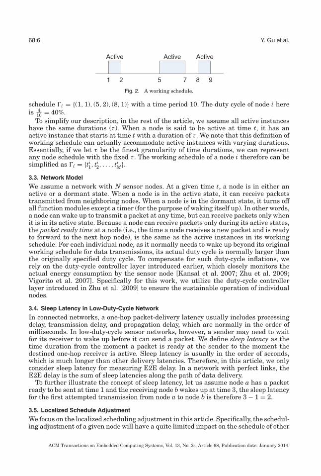
T . For example, Figure 2 shows a periodic working


68:6 Y. Gu et al.

Fig. 2. A working schedule.

schedule �i = {(1, 1), (5, 2), (8, 1)} with a time period 10. The duty cycle of node i hereis 4

10 = 40%.To simplify our description, in the rest of the article, we assume all active instances

have the same durations (τ ). When a node is said to be active at time t, it has anactive instance that starts at time t with a duration of τ . We note that this definition ofworking schedule can actually accommodate active instances with varying durations.Essentially, if we let τ be the finest granularity of time durations, we can representany node schedule with the fixed τ . The working schedule of a node i therefore can besimplified as �i = {ti

1, ti2, . . . , ti

M}.3.3. Network Model

We assume a network with N sensor nodes. At a given time t, a node is in either anactive or a dormant state. When a node is in the active state, it can receive packetstransmitted from neighboring nodes. When a node is in the dormant state, it turns offall function modules except a timer (for the purpose of waking itself up). In other words,a node can wake up to transmit a packet at any time, but can receive packets only whenit is in its active state. Because a node can receive packets only during its active states,the packet ready time at a node (i.e., the time a node receives a new packet and is readyto forward to the next hop node), is the same as the active instances in its workingschedule. For each individual node, as it normally needs to wake up beyond its originalworking schedule for data transmissions, its actual duty cycle is normally larger thanthe originally specified duty cycle. To compensate for such duty-cycle inflations, werely on the duty-cycle controller layer introduced earlier, which closely monitors theactual energy consumption by the sensor node [Kansal et al. 2007; Zhu et al. 2009;Vigorito et al. 2007]. Specifically for this work, we utilize the duty-cycle controllerlayer introduced in Zhu et al. [2009] to ensure the sustainable operation of individualnodes.

3.4. Sleep Latency in Low-Duty-Cycle Network

In connected networks, a one-hop packet-delivery latency usually includes processingdelay, transmission delay, and propagation delay, which are normally in the order ofmilliseconds. In low-duty-cycle sensor networks, however, a sender may need to waitfor its receiver to wake up before it can send a packet. We define sleep latency as thetime duration from the moment a packet is ready at the sender to the moment thedestined one-hop receiver is active. Sleep latency is usually in the order of seconds,which is much longer than other delivery latencies. Therefore, in this article, we onlyconsider sleep latency for measuring E2E delay. In a network with perfect links, theE2E delay is the sum of sleep latencies along the path of data delivery.

To further illustrate the concept of sleep latency, let us assume node a has a packetready to be sent at time 1 and the receiving node b wakes up at time 3, the sleep latencyfor the first attempted transmission from node a to node b is therefore 3 − 1 = 2.

3.5. Localized Schedule Adjustment

We focus on the localized scheduling adjustment in this article. Specifically, the schedul-ing adjustment of a given node will have a quite limited impact on the schedule of other



nodes. First of all, the schedule adjustment of a given node is only determined by itsown available energy, and thus the decision on whether the adjustment should be car-ried out is very localized. Second, the schedule adjustment of a given node only hasa very small impact on the operation of its predecessors and successors. To illustratethis, let us assume node b has augmented one active instance to its schedule, whichmeans its predecessor p has more chances to transmit packets to b, and thus mayconsume energy faster. However, these communication opportunities are utilized onlyif p has packets to send to b, while the number of packets that need to be transmittedis usually quite limited in low-duty-cycle sensor networks. As a result, the augmentingof active instances at node b only has a small impact on the energy consumption, andthus the active instances schedule, of its predecessor nodes. A similar conclusion canbe obtained for the successor nodes of b. The same reasoning holds when b decreases itsactive instances. Based on these two points, we can see that the schedule adjustmentof nodes is a very localized operation.

4. MODELING OF CROSS-TRAFFIC DELAY

4.1. Cross-Traffic Pattern

ESC is designed to be a flexible middleware between the network layer and MAC layerso that it can be used to support various existing routing protocols. Therefore, it isimportant to have a delay model that can capture the behavior of cross-traffic (many-to-many), a generalized case for one-to-one, many-to-one, and one-to-many traffic. Therelationship between the cross-traffic delay and E2E delay is further investigated inSection 9.4.

For a node b in the network, depending on the specific routing protocol adopted,there may be a set of nodes that forwards packets to node b, and we call those nodespredecessors of node b. Similarly, for different final destinations or multipath routingprotocols, node b would forward its packets to a certain set of nodes, and we call thosenodes successors of node b. For example, in Figure 3, the predecessors of node b includenode p1, p2, and p3, while the successors of node b are nodes s1 and s2. Here we notethat a node can be both a predecessor and a successor of node b, if this node exchangesdata bidirectionally with node b. For an individual node, by keeping track of sourceand destination node identification numbers of incoming and outgoing data packets,respectively, it can easily acquire and update its predecessor and successor list locally.

Note that although the modeling and design introduced in this and the followingsections are based on fixed predecessors and successors of a given node, nodes areable to perform adaptive ESC operation even when the routing paths change. Thisis because the ESC operation only requires localized input parameters, such as thepredecessors/successors of nodes and the percentage of the traffic through a node to itsgiven successor.

To model the cross-traffic delay at node b, we consider the expected delays for packetsfrom all predecessor nodes through node b, then to corresponding successor nodes.

4.2. Delay Modeling

Assume that at a predecessor node p1, a packet destined to node b is ready at time t,where t ∈ [0, T ]. Because the radio link between a pair of nodes is usually not perfect,node p1 may need to initiate multiple transmissions before the packet has successfullyarrived at node b. In order to obtain a corresponding sleep latency for each attemptedtransmission at node p1 after packet ready time t, we introduce a cycle representationof a node working schedule, shown in Figure 4.

In Figure 4, the cycle is equally divided by T ticks. Beginning at the 12 o’clock po-sition, the time increases from 0 to T clockwise. Consequently, we can easily label the


68:8 Y. Gu et al.

Fig. 3. Predecessors and successors. Fig. 4. A cyclic working schedule.

sequence of active instances at node b on the cycle. To measure the sleep latency (de-noted as L�b

t (k)) introduced by the working schedule of node b, for a given kth attemptedtransmission at time t, we can simply start from time t, follow the clockwise direction,and measure the total distance traversed by visiting k labels after time t on the cycle.For example, as depicted in Figure 4, where T is 10, units of time, the packet is readyat time t = 2 and node b wakes up during time 1, 3, 6, and 9. For the first attemptedtransmission (L�b

t (1)), the corresponding sleep latency is 1, because the total time tra-versed for visiting one label (tb

2 ) from time 2 is 1. Similarly, for the fourth attemptedtransmission (L�b

t (4)), the sleep latency is the total time traversed from t to tb2 , then to

tb3 , tb

4 and the fourth label tb1 , which gives 1 + 3 + 3 + 2 = 9 in total.

Link Reliability. Let the bidirectional link quality pab denote the success ratio of around-trip transmission (DATA and ACK) between node a and node b. The probabilitythat packet transmission succeeds at the kth attempt is the probability that previousk− 1 attempts failed times the probability that the current attempt succeeds, which issimply the link quality pab. Therefore, the probability that the packet reaches node bfrom node a at its kth attempt can be expressed as (1 − pab)k−1 pab.

Assuming the maximum number of packet transmission attempts within the networkis Rmax, for the packets arriving at node b from a, the probability that they arrive at thekth attempt is under the condition that the packet is delivered within Rmax transmissionattempts. The probability that a packet is delivered within Rmax transmission attemptscan be expressed as 1 − (1 − pab)Rmax , and the corresponding conditional probability canbe written as

Pab(k) = (1 − pab)k−1 pab

1 − (1 − pab)Rmax. (1)

Conditional Expected Delay Over a Single Link. For a packet ready time t at nodea, the expected transmission delay to reach node b is the sum of the product of theprobability that the packet reaches node b at its kth attempt and the correspondingsleep latency. Consequently, it can be formulated as

Dab(t) =Rmax∑k=1

Pab(k)L�bt (k). (2)

Conditional Expected Delay from One Predecessor to One Successors. For a packetready time t at a predecessor node pi, assuming the packet arrives at node b at thekth attempted transmission, its corresponding delay is simply L�b

t (k). Upon receivingthe packet at time t + L�b

t (k), node b would forward the received packet to a destinedsuccessor node sj with a delay of Dbsj (t + L�b

t (k)). Then the expected delay from prede-cessor pi to successor sj with packet ready time t at predecessor pi is the product of the



probability that the packet arrives node b at its kth attempted transmission and thecorresponding cross-traffic delay, which can be expressed as

D�bpisj

(t) =Rmax∑k=1

Ppib(k)(L�b

t (k) + Dbsj

(t + L�b

t (k)))

. (3)

Delay from Multiple Predecessors to Multiple Successors. To model the expected cross-traffic delay at node b from all packet ready times at all predecessor nodes to allsuccessor nodes, node b needs to know the portion of traffic that reaches node b fromeach packet ready time at all predecessor nodes to all successor nodes. To obtain thosestatistics, each predecessor of node b can piggyback the packet ready time for each sentpacket. Then at node b, with known sender and packet ready time for each packet, itcan easily keep track of what percentage of packets is from a given packet ready timet at a predecessor node pi, to a specific successor node sj . For each packet ready timetpik at a predecessor node pi, we can denote the percentage of its traffic through node

b to a successor node sj as W pisjk . Let the number of packet ready times at predecessor

node pi be Npi and the number of predecessor nodes and successor nodes at node b beNp and Ns, respectively, we can then express the expected delay of the cross-traffic atnode b with working schedule �b as

D�b =Np∑i=1

Ns∑j=1

Npi∑k=1

W pisjk D�b

pisj

(tpik

). (4)

The computational complexity of calculating the cross-traffic delay is determined byNp, Ns, Npi , and Rmax. It is clear that Npi and Rmax can not be excessively large inlow-duty-cycle sensor networks and are upper bounded with a specific network setting.Furthermore, it is clear that both Np and Ns are bounded by the node degree d. Thus,as a summary, the computational complexity of calculating D�b is O(d2). Note that dusually is also constrained, as will be explained next.

Next, we discuss the spatial complexity in calculating D�b. From Equation (4), we cansee that for node b to calculate D�b, it has to know the schedules of all its predecessorsand successors. If it takes 1 B of memory to store one active instance, a total amountof 1 × Mb = Mb B memory is needed to store the schedule of one node, where Mb isthe number of active instances of b, which is usually a small number in low-duty-cycle sensor networks. Thus, the total amount of memory for b to calculate D�b is1 × Mb(Np + Ns) = Mb(Np + Ns) when there is no overlapping between the sets ofpredecessors and successors of b, and smaller than this when the two sets overlap. It isclear that, asymptotically, Np + Ns ≤ 2d, where d is the average number of neighborsin the network, and is desirable to be small to reduce access contention [Gelal et al.2005]. On the other hand, the memory available for a typical MicaZ mote is 128 kB,in addition to a measurement flash of 512 kB. This available memory guarantees thefeasibility in the calculation of D�b.

5. ENERGY-SYNCHRONIZATION CONTROL

With the cross-traffic delay model available, we now introduce energy-synchronizationcontrol for minimizing communication delay. In this section, we first assume the work-ing schedules of predecessors and successors of a node are known and up to date. Later,in Section 6, we discuss the impact of obsolete schedules and methods for keeping theschedules up to date.


68:10 Y. Gu et al.

5.1. Main Idea

As shown in Section 2, energy harvested from surrounding environments varies signif-icantly over time at a sensor node. In order to make full use of the available energy sup-ply, we need to enhance system performance when there is abundant scavenged energyavailable; conversely, we need to decrease duty cycles with a minimum performancedegradation when there is a shortage in the power supply. Previous works [Kansalet al. 2007; Vigorito et al. 2007] have demonstrated methods for deciding the appropri-ate duty cycle of a sensor node with an in-situ energy supply. In this section, we furtherfocus on the impact of duty-cycle changes on communication delay. More specifically,when we increase the duty cycle of a node with additional available energy, we aimto minimize cross-traffic delay at the node. Similarly, when a node needs to decreaseits duty cycle due to insufficient energy supply, we would like to achieve a minimumincrease in the cross-traffic delay of the node. As a result, harvested energy at an indi-vidual node is synchronized by adjusting its duty cycle, with the objective of minimizingthe communication delay in the network.

5.2. Decrementing Single Active Instance

For a given node b, assume its working schedule is �b = {tb1 , tb

2 , . . . , tbMb

} and the energysupply can only afford Mb − 1 active instances to guarantee the sustainability of thenode. Therefore, we need to remove one active instance from node b’s working schedulesuch that the increase of cross-traffic delay at node b is minimized. Because sustainablesensor nodes work at extremely low duty cycles, the number of active instances in itsworking schedule is small and would always be below a constant value Mb ≤ T

τ.

Consequently, we can simply attempt to remove each of the existing active instances inthe sequence to find the optimal active instance for decrement, each with computationalcomplexity O(d2), as explained in Section 4.2, and select the one that yields minimalcross-traffic delay at node b. Therefore, the complexity of the optimal single activeinstance decrement is just O(d2).

5.3. Augmenting Single Active Instance

Intuitively, to augment one active instance at a node, we can perform an exhaustivesearch for all time instances within a round time T and choose the time instancethat yields a minimum cross-traffic delay at a node. Although this simple algorithm isacceptable, a much more efficient algorithm can be designed based on the stair effect,as presented in this section.

For a given node b, we can divide its time period into multiple intervals accordingto active instances of its predecessors and successors. Formally, we define an intervalas a time duration between two consecutive time instances from working schedules ofall predecessors and successors of node b on a cyclic working schedule. The summationof all intervals on a cyclic working schedule is equal to T . For example, as shownin Figure 5, assume the predecessor and successor of node b are node p and nodes, respectively. Let the active instances at node p and node s be {tp

1 , tp2 } and {ts

1, ts2},

respectively. According to their locations on the cyclic working schedule, we can easilyobtain four intervals for this specific scenario, namely: (tp

1 , ts1), (ts

1, tp2 ), (tp

2 , ts2), and (ts

2, tp1 ).

Intuitively, one would expect the timing of an augmented active instance within aninterval to yield different cross-traffic delays. However this is not the case. We observethat given schedules of predecessors and successors of node b, cross-traffic delay at nodeb depends only on the counts, instead of timing, of active instances within each interval.

To validate this observation, it is sufficient to prove that for two arbitrary layouts ofactive instances of the same size within an interval, the cross-traffic delays at node bare the same if packets are received within this interval.



Fig. 5. Period partition example. Fig. 6. Delay difference example.

LEMMA 5.1. For any packet ready time t at a predecessor node of node b, let X ={x1, x2, . . . , xm} and Y = {y1, y2, . . . , yn} be two sets of active instances of node b withinthe same interval starting at t (t < x1 < x2 < · · · < xm < t + t′ and t < y1 < y2 <· · · < yn < t + t′), where t + t′ is the end of the current interval determined by the activeinstances of the predecessor and successor (as shown in Figure 5). Let DX and DY becorresponding cross-traffic delays. Then DX = DY if m = n.

PROOF. For any packet ready time t at a predecessor node p, because x1, x2, . . . , xmand y1, y2, . . . , ym are in the same interval, as shown in Figure 6, the difference of sleeplatencies for the ith attempted transmission for X and Y after time t is just the differenceof their respective active instances. Consequently, if m = n, then LX

t (i) − LYt (i) = xi − yi,

for any 1 ≤ i ≤ m.Similarly, because xi and yi are within the same interval, the jth attempted trans-

mission from either xi or yi reaches the same active instance at a successor node s. Asclearly shown in Figure 6, if m = n, then L�s

xi( j) − L�s

yi( j) = yi − xi, where 1 ≤ i ≤ m and

1 ≤ j ≤ Rmax.By applying Equation (3) to X and Y , we have

DXps(t) − DY

ps(t) =Rmax∑i=1

Ppb(i)(LX

t (i) − LYt (i) + Dbs

(LX

t (i)) − Dbs

(LY

t (i)))

=Rmax∑i=1

Ppb(i)(xi − yi + Dbs(xi) − Dbs(yi)), (5)

since

Dbs(xi) − Dbs(yi) =Rmax∑j=1

Pbs( j)(L�s

xi( j) − L�s

yi( j)

) =Rmax∑j=1

Pbs( j)(yi − xi).

As∑Rmax

j=1 Pbs( j) = 1, we have

Dbs(xi) − Dbs(yi) = yi − xi. (6)

Consequently,

DXps(t) − DY

ps(t) =Rmax∑i=1

Ppb(i)(xi − yi + yi − xi) = 0. (7)

As a linear combination of DXps(t)− DY

ps(t) for all packet ready times at all predecessornodes, we have DX − DY = 0.


68:12 Y. Gu et al.

Fig. 7. Stair effect of cross-traffic delay.

Note that the requirement on m = n in Lemma 5.1 always holds when augmentingan active instance to the schedule of a node. Specifically, given a specific node b, m =n = Mb, where Mb is the number of active slots in b’s current schedule.

According to this observation, when augmenting one active instance within a par-titioned time interval, the cross-delay at node b is not affected by the timing of theaugmented active instance. In other words, single active-instance augmentation yieldsthe same cross-traffic delay at node b within each of partitioned time intervals. Conse-quently, for a single active-instance augmentation, we have a stair effect of cross-trafficdelays at node b within each partitioned time interval. Based on this counterintuitiveobservation, we can have the following theorem on finding the optimal single active-instance augmentation for minimizing cross-traffic delay at node b.

THEOREM 5.2. Assuming there are c intervals partitioned by the active instances atpredecessors and successors of node b, and xi is a random active instance within intervali (i = 1, 2, . . . , c). Let D�b

⋃{ j} represent the cross-traffic delay at node b after augmentingan active instance j to its original working schedule, and k = arg mini D�b

⋃{xi}, then anytime instance within interval k is the optimal single active-instance augmentation, andthe complexity of this process is O(d3), where d is the average number of neighbours inthe network (network density).

PROOF. Denote M as the average number of active slots of nodes. We need O(log(dM))time to identify all the c intervals, which can be done by sorting all the active slots of b’sneighbors. Within any time interval i and for any random augmented active instancexi, we essentially increase the number of active instances within the interval by one. ByLemma 5.1, to find the optimal augmented active instance at a node, we simply needto check the cross-traffic delay with a random active-instance augmentation withineach of the time intervals and find the interval k that yields the minimum cross-trafficdelay. Because sustainable sensor networks operate at extremely low duty cycles, thepacket ready times from predecessor nodes and active instances from successor nodesare quite limited. Thus the complexity of finding the optimal active instance is justO(d2(log dM + c)). Considering the fact that c ≤ dT

τ, the complexity can be represented

by O(d3).

To further illustrate Theorem 5.2, we give an example in Figure 7. Assuming oneperiod time contains 200 time instances, Figure 7 shows the expected cross-traffic delayat a node for different augmented active instances. For example, the delay correspond-ing to active instance 1 represents the delay at node b after augmenting an activeinstance at time 1. The node shown in Figure 7 has a predecessor with active instances(36, 53, 80) and a successor with active instances (90, 151, 189). According to our pre-ceding analysis, we can divide one time period into the following intervals: (36, 53),(53, 80), (80, 90), (90, 151), (151, 189), (189, 36). From Figure 7, it is clear that we havea stair effect of delays at the node among these time intervals, which is consistent with



our analysis. The optimal augmented active instance, therefore, is any value withininterval (80, 90).

5.4. Bursty Augmentation and Decrementation

In the previous two sections, we introduced optimal solutions for augmenting anddecreasing a single active instance for the scenario that energy variation is slow. How-ever, the change in the harvested energy could be bursty, and therefore, a node mayneed to increase or decrease multiple active instances simultaneously. In this section,we present a minimal cost solution for augmenting and decreasing multiple activeinstances.

For multiple active-instance augmentation and decrementation, the exhaustivesearch approach is no longer acceptable, because the computational complexity growsexponentially with the number of augmented or decreased instances. Therefore, a low-cost solution with guaranteed optimality in performance is desirable. Fortunately, weobserve that the multiple active-instance augmentation and decrementation can beoptimally solved with a greedy approach.

THEOREM 5.3. The optimal solution for augmenting/decreasing u active instances ata node can be obtained by applying the single active-instance augmentation/decrement-ation u times.

Because the computational complexity of single active-instance augmentation ordecrement is O(d3) and O(d2), respectively, the corresponding complexity for augment-ing or decrementing u active instances is O(ud3) and O(ud2).

6. MAINTAINING LOGICAL CONNECTIVITY

In the previous section, energy-synchronization control is designed to adjust the work-ing schedules at receiving nodes, assuming the schedule of predecessors and successorsare known and up to date. In this section, we investigate the impact of obsolete sched-ules and how to maintain connectivity while updating schedules.

6.1. Impact of Schedule Updates

To understand how obsolete schedules can affect the connectivity between nodes, letus consider an example where the working schedule of node b has been changed buthas not yet been updated to its predecessor node p.

—Unnecessary Loss. If node b decreases its duty cycle due to insufficient energy supply,then one or more original active instances at node b may be removed. However, beforenode p is updated, it would continue to deliver packets according to the old (obsolete)working schedule of node b, which could suffer significantly greater packet loss thannecessary.

—Suboptimal Delay. If node b increases its duty cycle and a predecessor node is un-aware of the augmented active instances at node b, it would continue to deliver thepackets at node b’s original active instances. In addition, for both predecessors andsuccessors, the new schedule of node b is essential for them to perform effective en-ergy synchronization. Therefore, it is crucial for node b to promptly disseminate itsnew working schedule to its predecessor and successor nodes.

6.2. Reactive vs. Proactive Updates

In order to inform predecessor nodes or successor nodes of its new working schedule,node b can either proactively notify them immediately after its duty-cycle synchroniza-tion or reactively send its new schedule to nodes with which it has ongoing communica-tion. Specifically, for proactive notification, node b generates one packet that contains


68:14 Y. Gu et al.

Fig. 8. Comparison of logical connectivity.

its new schedule for each of its predecessor and successor nodes and tries to deliver allthose packets according to the active instances of predecessor and successor nodes. Incontrast, for a reactive update, node b only sends its new schedule to a predecessor ora successor if the predecessor sends a packet to node b or node b sends a packet to thesuccessor nodes.

Obviously, the advantage of proactive notification is that predecessors and succes-sors can receive the new working schedule of node b promptly. However, proactivelysending schedule update packets to all predecessors and successors increases the traf-fic load within the network and consequently increases the chances of collisions andinterferences within the network. More importantly, if there is no traffic flow betweena predecessor/successor and node b during two or more node working schedule up-dates, sending those schedule updates would waste energy. In contrast, if adoptinga reactive schedule update, node b only sends the new schedule to predecessors orsuccessors with which it has communication, therefore minimizing the chance of send-ing unnecessary schedule updates due to the well-known temporal and spatial local-ity for traffic flow in communication networks. As a result, in this work, we recom-mend the reactive schedule update for the dissemination of new working schedules ofnode b.

6.3. Shuffle-Based vs. Adjustment-Based Energy Synchronization

Generally, two approaches can be adopted when node b increases or decreases its dutycycles. Node b can either generate a completely new working schedule with a new givenenergy budget (termed a shuffle), or node b can increase or decrease its duty cycle ontop of its previous working schedule (termed an adjustment).

To facilitate the comparison of shuffle-based and adjustment-based energy synchro-nization, we first present two types of connectivities in duty-cycled sensor networks,namely, the physical connectivity and logical connectivity. Two nodes are physicallyconnected if they are within each other’s communication range and logically connectedonly if they can communicate. Unlike traditional networks, a low-duty-cycle networkcould be physically connected but logically partitioned if nodes do not know each other’sworking schedules.

Let logical connectivity �ab be the packet delivery ratio between two nodes a andb, after Rmax retransmissions. Let �b be the set of first Rmax active instances in theoriginal schedule and �′

b be the new schedule of node b. The logical connectivity �abwhen b switches from �b to �′

b, therefore, is

�ab = 1 − (1 − pab)K where K = |�b ∩ �′b|. (8)

6.3.1. Comparison. In this section, we investigate the performance of shuffle and ad-justment in terms of logical connectivity and cross-traffic delay. The simulation setup isthe same, as described in Section 9. Figure 8 shows the percentage of the old working



Fig. 9. Comparison of delay beforeschedule update.

Fig. 10. Comparison of delay af-ter schedule update.

Fig. 11. Delay vs. energy varia-tion rate.

schedule that is preserved after schedule synchronization using shuffle and adjust-ment. Clearly, adjustment preserves a much larger portion of the old working schedulethan shuffle does for all node duty cycles. As the node duty cycle increases, the per-centage of the working schedule preserved in an adjustment increases while that for ashuffle decreases. This is because with the increasing duty cycle at a node, the effectof adjusting the node working schedule is constantly reduced, while a shuffling of theworking schedule could result in increasing deviations between the old and new work-ing schedules. For example, the percentage of the working schedule preserved in anadjustment increases from 90.1% to 96.4% when the duty cycle increases from 1% to5%. In contrast, shuffling decreases the percentage from 26% to 13.5%. Because logicalconnectivity is decided by the intersection of old and new working schedules at a node,Figure 8 confirms that adjustment maintains a significantly better logical connectivitythan that of the shuffle.

Before the new working schedule of a node reaches its predecessors, the traffic delayfrom the predecessor nodes is dominated by the logical connectivity. Figure 9 shows thetraffic delay for shuffle and adjustment before the new energy-synchronized workingschedule reaches the predecessor nodes in a randomly generated network. Figure 9clearly indicates that because adjustment maintains a much better logical connectivitythan shuffle, a pair-wise comparison of delays at each node shows that adjustmentproduces much smaller delays than shuffle. For example, the average delays for anadjustment and a shuffle are 252.79 and 711.2 units of time, respectively.

After the new working schedule of a node reaches its predecessors, a shuffle wouldachieve the optimal expected delay, because it creates a completely new working sched-ule that minimizes cross-traffic delay at the node. Figure 10 shows cross-traffic delaysafter a new working schedule has reached predecessor nodes. As expected, shuffleyields smaller delays than adjustment at all nodes. For example, the average delay foradjustment and shuffle is 239.26 and 213.07 units of time, respectively.

Because adjustment produces smaller delays before the new working schedulereaches predecessor nodes and shuffle creates smaller delays after the new work-ing schedule reaches predecessor nodes, the overall delay at a node is influenced bythe energy variation at the node. To further investigate the influence of energy diver-sity on the delay, we introduce the energy-variation rate as a new parameter in thesimulation, which is defined as the average number of times that a node increases ordecreases its duty cycle over a period of 100,000 units of time. Figure 11 shows averagecross-traffic delays for both adjustment and shuffle under different energy-variationrates. When the energy-variation rate is low, the delay after schedule disseminationdominates the overall delay, and therefore, shuffle has a smaller overall delay thanthat of adjustment. For example, when the energy variation rate is 1, the overall de-lay for adjustment and shuffle is 226.34 and 206.17 units of time, respectively. As theenergy variation rate becomes larger, the delay before schedule dissemination weightsmore in overall cross-traffic delay. Consequently, adjustment that has a smaller delaybefore schedule dissemination also has a smaller overall delay than shuffle. As shown


68:16 Y. Gu et al.

in Figure 11, from energy variation rate 2.5 to 5, adjustment has a smaller delay thanthat of shuffle. At energy-variation rate 5, the delay for adjustment and shuffle is225.22 and 257.65 units of time, respectively. In addition, the amplitude of duty-cyclechanges also has a similar impact, as we can convert such changes of amplitude to thefrequency of changes. This study indicates that the design options on ESC should bedecided based on how fast and how much ambient energy changes over time.

7. PRACTICAL ISSUES

This section completes our ESC design by discussing several practical design issues,such as time synchronization and multiple transmissions within a time instance.

7.1. Low-Cost Time Synchronization

For the sake of clarity, we introduce the ESC design in a synchronized mode. Clearly, theoperation of ESC depends on neither neighbor time instance nor global synchronization.It is sufficient for ESC to know only the wake-up time interval of predecessor andsuccessor nodes. To know those wake-up time intervals, simple and low-cost localsynchronization techniques [Maroti et al. 2004] can achieve an accuracy of 2.24μswith the cost of exchange being a few bytes of packets among neighboring nodes every15 minutes. Because an active instance typically ranges from 2,000μs to 20,000μs, theaccuracy of 2.24μs is far more than sufficient. In addition, ESC does not require thatthe transmission starts at the beginning of an active instance, which further relaxesthe requirement of accuracy for time synchronization.

7.2. Multiple Transmissions within a Time Instance

While describing our network model in Section 3, we assume there is at most onepacket transmission during an active instance. This is true if nodes are equipped withslow radio. However, if a fast radio is used, it is possible to transmit multiple packetswithin an active instance. To accommodate such scenarios in the modeling of cross-traffic delay, we can simply rewrite the bidirectional link quality between two nodes asp′

ab = 1 − (1 − pab)m, where m is the maximum number of transmissions allowed in anactive instance. Essentially, the new p′

ab represents the probability that the receiverreceived the packet by m transmissions.

8. IMPLEMENTATION AND EVALUATION

In order to validate the performance and feasibility of ESC in practice, we fully im-plement ESC on the TinyOS-2.1/Mote platform in nesC. To compare the performanceof ESC, we also implement a random schedule-synchronization scheme that randomlyadjusts active instances of the original node working schedule with increasing or de-creasing node duty cycles.

8.1. Experiment Setup

In the experiment, 30 MicaZ nodes are randomly placed in our testbed, which canaccommodate at most 360 sensor nodes. The transmission power at MicaZ motes istuned down to −24dBm (by setting the power level as 3) to form a multihop net-work. To reduce the implementation overhead, we synchronize neighboring nodes usingFTSP [Maroti et al. 2004], which is a standard component in TinyOS 2.1. The lengthof each active instance is set to 20ms. The available energy budget over time at eachnode is derived from the actual energy-harvesting profile measured at our runningprototype [Zhu et al. 2009]. The range of duty cycles varies from around 0.2% to 10%.According to the available energy budget, each node turns on or off its radio based on the



Fig. 12. ETX topology. Fig. 13. DESS topology.

Fig. 14. ETX E2E delay. Fig. 15. DESS E2E delay.

energy-synchronized working schedule. To investigate the flexibility of the ESC design,we choose two state-of-the-art solutions as underlying routing protocols:

—Link-Quality-Based. ETX [Couto et al. 2003].—Sleep-Latency-Based. DESS [Lu et al. 2005].

8.2. Performance Comparison

In this section, we compare the E2E delay for both ESC and the randomized scheme.During the experiment, over 1,000 packets for each routing protocol are transmittedfrom a random source to the sink, which is randomly selected from the 30 motes andkept fixed during the evaluation. To minimize the impact of temporal energy variationand link quality fluctuation, nodes in the network periodically switch between ESCand randomized energy-synchronization protocols so as to ensure fair performancecomparisons.

In Figure 12 and Figure 13, we plot two snapshots of the routing topologies for bothETX and DESS on our testbed. From Figure 12 and Figure 13, we can see the routingtopology significantly varies for ETX and DESS, even for a 30-node testbed.

In Figure 14, we study the E2E delay for ESC and the randomized scheme underETX. Clearly, ESC performs much better than the randomized scheme. While 80% ofESC packets reach their destinations within 877ms, the corresponding percentile forthe randomized scheme is 1,451ms, which is about a 65% increase. Because ETX picksthe route with the minimum number of expected transmissions, the performance gapbetween ESC and the randomized scheme, therefore, is mainly due to the minimizedcross-traffic delay for ESC.

Similar to the results for ETX, ESC also significantly outperforms the randomizedscheme under DESS in Figure 15. While the 80th percentile for ESC is 1,131ms, thecorresponding delay for the randomized scheme is 2,091ms, which almost doubles thedelay of ESC. In addition, the randomized scheme has a much longer tail than ESC.While all packets for ESC reach the destinations within 6,299ms, the longest E2Edelay for the randomized scheme is 12,343ms. The reason for such a long tail of therandomized scheme is because the penalty of a failed transmission for the randomizedscheme is much larger than for ESC, as ESC has carefully scheduled the radio activityto minimize the impact of the failed transmissions.


68:18 Y. Gu et al.

Fig. 16. Node duty cycle over time. Fig. 17. Cross-traffic delay over time.

To further reveal the performance of ESC over the time dimension, Figure 16 andFigure 17 show the duty cycle of a deployed node and its corresponding cross-trafficdelay under ESC and the randomized scheme over a period of three hours. By comparingFigure 16 and Figure 17, we can see the cross-traffic delay matches the available dutycycle well. For example, the peaks of delay occur when the node duty cycle drops toaround 0.4% at time 65 and 100. In addition, although both ESC and the randomizedscheme react to the duty-cycle change promptly, the cross-traffic delay for ESC is alwayssmaller than that of the randomized scheme. This consistently smaller cross-trafficdelay of ESC over time further explains the smaller E2E delay for ESC in Figure 14.

9. SIMULATION EVALUATION

In addition to testbed evaluations in Section 8, in this section, we provide simulationresults with over 4,000 sensor nodes to understand the system performance of ESCunder various network settings.

9.1. Simulation Setup

In the simulation, except where otherwise specified, we deploy up to 4,200 sensornodes randomly in a 400m × 400m square field. A sink is positioned in the centerof the field, and each sensor node sends its packet to the sink over multiple hops.The communication range of sensor nodes is 25m. The radio model was implementedaccording to Zuniga and Krishnamachari [2004], which considers the oscillatory natureof the radio links and has several adjustable parameters. During the simulation, weset these parameters strictly according to the CC2420 radio hardware specification[CC2420 2012]. Specifically, the PRR (packet reception rate) for a link of length d isgiven by

P RR(d) =(

1 − 12

exp− γ (d)2

10.64

)8 f

, (9)

where γ (d) is the SNR (signal-to-noise ratio), which can be determined by the RSSImeasurements, and f is the frame size. The RSSI readings are simulated as Gaussiandistributed variables whose mean is determined by the path-loss model with a path-lossexponent of 3.0, and the shadowing standard deviation is set to 3.8. The frame size isset to 50B. Identical to the testbed evaluation, the energy model used in the simulationevaluation is also based upon our empirical measurement and energy-harvesting model[Zhu et al. 2009].

Each experiment was repeated 100 times with different random seeds, node de-ployments, and node harvested energy. Data collected at each node were obtained byaveraging over 10,000 source-to-sink communications. The 95% confidence intervalsare within 1∼4% of the mean.



Fig. 18. Delay over time.

Fig. 19. Performance of shuffle vs. adjustment under different maximum retransmissions.

9.2. System Performance over Time

In this section, we reveal the effectiveness of ESC over time in terms of communicationdelays. Figure 18 shows the average cross-traffic delay at a node over a period of 25,000units of time. At time 0, active instances are allocated randomly within nodes (hence,not optimally). The node increases its duty cycle at time 5,000 and 10,000 and decreasesits duty cycle at time 15,000 and 20,000. It is clear that after the node increases itsduty cycle at time 5,000, the delay at the node significantly drops. For example, withintime interval [0, 5000], the average delay is 249.26 units of time. In contrast, duringtime [5000, 10000], the average delay drops to 90.51, which is around only 36.3% ofthe original delay. After increasing the duty cycle again at time 10,000, the delay atthe node further reduces to 50.32 during time [10000, 15000], almost half the previousdelay. When the duty cycle decreases at time 15,000, the average delay only slightlyincreases to 51.36 units of time within time interval [15000, 20000]. Finally, when wefurther reduce the duty cycle at time 20,000, the delay increases to 113.66, which isonly around 45.6% of the initial delay during time [0, 5000], when allocation is notoptimal. From this figure, it is clear that ESC effectively reduces the delay at the nodewhen its duty cycle increases, while it minimally increases the delay when the nodedecreases its duty cycle, converging gradually from an initial suboptimal allocationinto an optimal allocation.

9.3. Comparing Shuffle with Adjustment

Previously, we discussed the per-hop delay impact of shuffle and adjustment. In thissection, we systematically compare the system performance for adjustment-based andshuffle-based energy-synchronization methods in terms of multihop E2E data-deliverydelay and data-delivery ratio.

In both Figure 19 and Figure 20, we deploy sensor nodes in a 150m × 150m areawith an average 1% node duty cycle. The energy-variation rate, which is defined inSection 6.3.1, is set to be 1 here, which favors shuffle for the single-hop scenario.Figure 19 shows the E2E delay and data delivery ratio for adjustment and shuffle underdifferent maximum numbers of retransmissions. From Figure 19, we can see that under


68:20 Y. Gu et al.

Fig. 20. Performance of shuffle vs. adjustment under different node densities.

all maximum number of retransmissions, adjustment has a smaller delivery delay and alarger delivery ratio than does the shuffle. For example, when the maximum number ofretransmissions is three within the network, the average delay for adjustment is 648.6units of time, while the delay for shuffle is 699.2 units of time—an 8% difference. Forthe data delivery ratio, under three maximum number of retransmissions, adjustmentdelivers 86% of data, while shuffle delivers only around 70% of messages. Similarly, inFigure 20, adjustment outperforms shuffle in terms of delivery delay and delivery ratiofor all node densities.

By comparing the performance of these two schedule update approaches, it is clearthat adjustment is favorable in a multihop network. This is because as network sizeincreases, the impact of inconsistent views of node working schedules at individualhops along the data path increases exponentially for E2E delays in the network.

9.4. Impact of Changing Cross-Traffic Delay on the Path Delay

For our ESC design, in order to provide a transparent middleware and support variousexisting routing protocols, we focus on minimizing the cross-traffic delay at individualnodes. However, it is also essential to study the effectiveness of reducing cross-trafficdelay on the actual E2E communication delays. To reveal the correlation of delayreductions for cross-traffic delays and corresponding E2E path delays, Figure 21 plotsthe expected delay reduction from cross-traffic delays and actual E2E path delaysunder different numbers of active instance augmentations. From Figure 21, we cansee the reduction of expected cross-traffic delay at individual nodes indeed leads tothe reduction of E2E path communication delays. In addition, from Figure 21, wecan observe that the expected delay reductions from expected cross-traffic delays atindividual nodes along the E2E communication path fairly accurately predict the actualE2E delay reductions. Consequently, we can conclude that the cross-traffic delay atindividual nodes along a path are positively correlated with the E2E communicationdelay and can fairly accurately predict the E2E delay changes along the path.

9.5. Comparison with Global Synchronization

To demonstrate the advantage of energy synchronization, we compare ESC with theglobal synchronization, where the active-instance schedule of nodes does not changewith the energy supply. In the global synchronization, each node is labeled according toits hop count from the sink, and the route path is constructed based on the label. For thepurpose of a fair comparison, the duty cycle of nodes in the global synchronization is setto the average duty cycle of nodes in ESC, or more specifically, 1.5% in our simulation.The comparison results are shown in Figure 22. Not surprisingly, we can see that bothESC and the randomized schedule adjustment outperform global synchronization. Thisdemonstrates the advantages of the adaptive scheduling adjustment over the fixedscheduling. To be explicit, the reduction in the communication delay with ESC and



Fig. 21. Number of active-instance augmenta-tions vs. delay reduction.

Fig. 22. Comparison with global synchroniza-tion.

Fig. 23. E2E delay vs. data rate.

the randomized adjustment, when compared with global synchronization, is around30%–40% and 50%–60%, respectively.

9.6. Impact of MAC Layers

In this section, we study the impact of MAC-layer protocol selection on the E2E commu-nication delays for ESC. Specifically, we are interested in seeing the performance differ-ence between sender-initiated MAC protocols (B-MAC [Polastre and Culler 2004]) andreceiver-initiated MAC protocols (A-MAC [Dutta et al. 2010]). Figure 23 shows the E2Edelay of sender-initiated MAC and receiver-initiated MAC under different data ratesin energy-harvesting sensor networks. From Figure 23, we can see receiver-initiatedMAC protocols are generally more preferable for low-duty-cycle energy-harvesting sen-sor networks, especially when the data rate in the network is high. This is because inlow-duty-cycle networks, a sender of sender-initiated MAC protocols, such as B-MAC,sends long preambles to ensure successful communications with its intended receiver,and such long preambles suppress other potential communications in the surround-ing area. In contrast, a node of receiver-initiated MAC protocols, such as A-MAC,listens only to the probe message from its intended receiver and does not interfere withother potential communications from neighboring nodes. Therefore, we would recom-mend the adoption of well-implemented sender-initiated MAC protocols over widelyused sender-initiated MAC protocols for low-duty-cycle energy-harvesting sensornetworks.

9.7. Impact of Node Densities

In this section, we examine the impact of node densities on E2E delay for both ETXand DESS networks with varying energy supplies over time. During the simulation,the energy profiles for specific nodes are the same for ESC and the randomized energysynchronization scheme to ensure fair comparison. As can clearly be seen from bothFigures 24(a) and 24(b), ESC has a much smaller delay than the randomized scheme atall node densities for both ETX and DESS. For example, at node density 30, ETX-ESC


68:22 Y. Gu et al.

Fig. 24. Impact of node densities (ESC vs. randomized control).

Fig. 25. Impact of node harvested energy (ESC vs. randomized control).

has a delay of 538 units of time, while ETX-Random has a delay of 809 units of time,which is about 50% larger than the delay for ETX-ESC.

9.8. Impact of Node Harvested Energy

In this section, we study the impact of node harvested energy on E2E delay by applyingESC to ETX and DESS in energy-varying sustainable sensor networks. For this specificevaluation, we tweak the energy-harvesting model so as to get the desired averagenode harvested energy for each experiment. In both Figures 25(a) and 25(b), we cansee that ESC outperforms the randomized scheme at all node harvested energies. Asthe node harvested energy increases, E2E delays for both ETX and DESS under ESCand the randomized scheme are decreasing. This is because with a higher node energy-harvesting rate in the network, the sleep latency between a sender and a receiver isreduced, as there are more active instances for the receiver to receive incoming packetsfrom sending nodes.

10. RELATED WORK

Several technologies have been developed to extract energy from the environment, in-cluding solar, motion, biochemical, and vibrational [Meninger et al. 1999; Wright et al.2000]. Building on those energy-harvesting technologies, researchers have designedvarious types of platforms to collect ambient energy from the environment with op-timal efficiency [Dutta et al. 2006; Rahimi et al. 2003; Jiang et al. 2005; Gorlatovaet al. 2009]. To fully utilize the harvested energy and ensure the sustainable operationof sensor nodes, Kansal et al. [2007] and Vigorito et al. [2007] have presented boththeoretical and experimental results on deciding the appropriate working duty cycleof sensor nodes with information on current energy-harvesting rates. To further studythe impact of energy leakage for energy-harvesting sensor networks, the TwinStar sys-tem suggests node duty cycles based on user-specified lifetime and energy information,including energy-harvesting rate, remaining energy in the system and energy-leakage



rate [Zhu et al. 2009]. To explore collaborative energy management, IDEA [Challenet al. 2010] allows individual nodes to evaluate their own impact on other nodes andenables awareness of the connection between the behavior of each node, the applica-tion’s energy goals, and system performance.

MAC-layer design has been a major focus for supporting low-duty-cycle networking.In general, existing MAC protocols can be categorized into two categories. One categoryis synchronous MAC protocols, including S-MAC [Ye et al. 2002], T-MAC [van Dam andLangendoen 2003], RMAC [Du et al. 2007], and DW-MAC [Sun et al. 2008a], whichsynchronize neighboring nodes in order to align their active or sleeping periods. Theother category is asynchronous MAC protocols, including B-MAC [Polastre and Culler2004], X-MAC [Polastre and Culler 2004], WiseMAC [El-Hoiydi and Decotignie 2004],RI-MAC [Sun et al. 2008b], and A-MAC [Dutta et al. 2010], which allow the sensornode to operate individually with its own working schedule through techniques suchas Low-Power-Listening. More recently, some hybrid MAC protocols, such as SCP-MAC [Ye et al. 2006], Z-MAC [Rhee et al. 2008], and Funneling-MAC [Ahn et al. 2006],are designed to take advantage of two traditional approaches. On top of MAC protocolsthat focus on allowing multiple sensor nodes to share the physical medium, ESC aimsto capture the most generic many-to-many communication pattern and minimize thecross-traffic delay at individual nodes.

Due to the growing gap between limited energy and increasing energy demand inlong-term applications, there has been a surge of research interest in low-duty-cyclenetworking. For scenarios with mobile nodes, a number of effective solutions hasbeen proposed for data communication [Lindgren et al. 2004; Spyropoulos et al. 2008;Musolesi et al. 2005]. For scenarios with low-duty-cycle nodes, by assuming perfectlink qualities, both Lu et al. [2005] and Keshavarzian et al. [2006] introduce severaltechniques for minimizing communication latency while providing energy-efficientperiodic node working schedules. To address both low-duty-cycle and unreliablecommunication links, Gu and He [2007] introduce a dynamic switch-based forwardingusing optimized forwarding sequences. Su et al. [2008] propose both on-demand andproactive algorithms for routing packets in low-duty-cycle networks. Efficient floodingprotocols have been introduced to tackle the challenges in low-duty-cycle sensornetworks [Guo et al. 2009; Wang and Liu 2009]. More recently, Gu et al. [2009a]studied the delay control for low-duty-cycle sensor networks.

Routing algorithms incorporating the energy-harvesting feature exist in the litera-ture [Lattanzi et al. 2007; Lin et al. 2007; Hasenfratz et al. 2010]. A methodology forassessing the energy efficiency of routing algorithms for energy-harvesting networksis proposed in Lattanzi et al. [2007]. Lin et al. model and characterize the performanceof multihop radio networks in the presence of energy constraints [2007]. A modifiedversion of the R-MPRT algorithm is proposed in Hasenfratz et al. [2010]. These ex-isting results mainly focus on the energy-aware optimal routing design, and our workadvances the state of the art by optimizing the network performance in the time di-mension, thus complementing the existing achievements.

However, none of those prior works investigate how changing the duty cycle of sensornodes affects communication performance in sustainable sensor networks and how wecan adaptively synchronize node working schedules with specified duty-cycle budgets.Acting as a transparent middleware service between the MAC layer and network layer,ESC adjusts only RF activities at individual nodes while taking routing- and link-quality information from those two layers for minimizing cross-traffic delays. In thiswork, we advance state-of-the-art solutions for both energy-harvesting and low-duty-cycle sensor networks and provide effective methods of synchronizing node workingschedules with varying duty-cycle budgets.


68:24 Y. Gu et al.

11. CONCLUSION

In this work, we reveal that cross-traffic delay through a duty-cycled node is determinedonly by the number of active instances at intervals, partitioned by active instances ofpredecessor and successor nodes. This allows us to design energy-synchronized controlwith O(d3) time complexity for sustainable networks in which energy supplies anddemands are in balance, where d is the node degree in the network. In a low-duty-cyclenetwork, updating neighbors’ working schedules would be slow, leading to inconsistentviews on active instances. To address this issue, we investigate the impact of obso-lete working schedules on logical link quality and demonstrate the trade-off betweenshuffle-based and adjustment-based allocation under different energy variation rates.Our evaluation demonstrates that ESC can effectively reduce delay and increase de-livery ratios while synchronizing radio activity with available energy.

REFERENCES

Gahng-Seop Ahn, Se Gi Hong, Emiliano Miluzzo, Andrew T. Campbell, and Francesca Cuomo. 2006.Funneling-MAC: A localized, sink-oriented MAC for boosting fidelity in sensor networks. In Proceedingsof the 4th ACM Conference on Embedded Networked Sensor Systems (SenSys’06).

CC2420. 2012. CC2420 Product Information and Data Sheet. CC2420 2012. http://www.ti.com.cn/product/cn/cc2420.

Geoffrey Werner Challen, Jason Waterman, and Matt Welsh. 2010. Idea: Integrated distributed energyawareness for wireless sensor networks. In Proceedings of the 8th International Conference on MobileSystems, Applications, and Services (MobiSys’10).

Douglas S. J. De Couto, Daniel Aguayo, John Bicket, and Robert Morris. 2003. A high-throughput path metricfor multi-hop wireless routing. In Proceedings of the 9th International Conference on Mobile Computingand Networking (MOBICOM’03).

Shu Du, Amit Kumar Saha, and David B. Johnson. 2007. RMAC: A routing-enhanced duty-cycle MACprotocol for wireless sensor networks. In Proceedings of the 26th IEEE International Conference onComputer Communications (INFOCOM’07).

Prabal Dutta, Stephen Dawson-Haggerty, Yin Chen, Chieh-Jan Mike Liang, and Andreas Terzis. 2010.Design and evaluation of a versatile and efficient receiver-initiated link layer for low-power wireless. InProceedings of the 8th ACM Conference on Embedded Networked Sensor Systems (SenSys’10).

P. Dutta, J. Hui, J. Jeong, S. Kim, C. Sharp, J. Taneja, G. Tolle, K. Whitehouse, and D. Culler. 2006. Trio:Enabling sustainable and scalable outdoor wireless sensor network deployments. In Proceedings of the5th International Conference on Information Processing in Sensor Networks (IPSN’06).

A. El-Hoiydi and J.-D. Decotignie. 2004. WiseMAC: An ultra low power MAC protocol for the downlink ofinfrastructure wireless sensor networks. In Proceedings of the IEEE Symposium on Computers andCommunications.

Zhi Ang Eu, Hwee Pink Tan, and Winston Khoon Guan Seah. 2010. Opportunistic routing in wireless sensornetworks powered by ambient energy harvesting. Comput. Netw. 54, 17 (2010), 2943–2966.

X. Fafoutis and N. Dragoni. 2011. OdMAC: An on-demand MAC protocol for energy harvesting wirelesssensor networks. In Proceedings of the 8th ACM Symposium on Performance Evaluation of Wireless AdHoc, Sensor, and Ubiquitous Networks (PE-WASUN’11).

Ece Gelal, Gentian Jakllari, Srikanth V. Krishnamurthy, and Neal E. Young. 2005. Topology control tosimultaneously achieve nearoptimal node degree and low path stretch in ad hoc networks. In Proceedingsof the 2nd IEEE Communications Society Conference on Sensor and Ad Hoc Communications andNetworks (SECONÕ’05).

Maria Gorlatova, Peter Kinget, Ioannis Kymissis, Dan Rubenstein, Xiaodong Wang, and Gil Zussman. 2009.Challenge: Ultra-low-power energy-harvesting active networked tags (enhants). In Proceedings of theInternational Conference on Mobile Computing and Networking (MobiCom’09).

Yu Gu and Tian He. 2007. Data forwarding in extremely low duty-cycle sensor networks with unreliablecommunication links. In Proceedings of the 5th ACM Conference on Embedded Networked Sensor Systems(SenSys’07).

Yu Gu, Tian He, Mingen Lin, and Jinhui Xu. 2009a. Spatiotemporal delay control for low-duty-cycle sensornetworks. In Proceedings of the 30th IEEE Real-Time Systems Symposium (RTSS).

Yu Gu, Ting Zhu, and Tian He. 2009b. ESC: Energy synchronized communication in sustainable sensornetworks. In Proceedings of the IEEE International Conference on Network Protocols (ICNP’09).



Chao Gui and Prasant Mohapatra. 2004. Power conservation and quality of surveillance in target track-ing sensor networks. In Proceedings of the 10th International Conference on Mobile Computing andNetworking (MobiCom’04).

Shuo Guo, Yu Gu, Bo Jiang, and Tian He. 2009. Opportunistic flooding in low-duty-cycle wireless sensornetworks with unreliable links. In Proceedings of the International Conference on Mobile Computingand Networking (MobiCom’09).

David Hasenfratz, Andreas Meier, Clemens Moser, Jian jia Chen, and Lothar Thiele. 2010. Analysis, compar-ison, and optimization of routing protocols for energy harvesting wireless sensor networks. In Proceed-ings of the IEEE International Conference on Sensor Networks, Ubiquitous, and Trustworthy Computingand the IEEE International Workshop on Ubiquitous and Mobile Computing (SUTC/UMC).

Shibo He, Jiming Chen, David Yau, Huanyu Shao, and Youxian Sun. 2009. Energy-efficient capture ofstochastic events by global- and local-periodic network coverage. In Proceedings of the 10th ACM Inter-national Symposium on Mobile Ad Hoc Networking and Computing (MobiHoc).

Anh Tuan Hoang and Mehul Motani. 2007. Collaborative broadcasting and compression in cluster-basedwireless sensor networks. ACM Trans. Sens. Netw. 3, 3.

X. Jiang, J. Polastre, and D. Culler. 2005. Perpetual environmentally powered sensor networks. In Proceed-ings of the 4th International Symposium on Information Processing in Sensor Networks (IPSN’05).

Aman Kansal, Jason Hsu, Sadaf Zahedi, and Mani B. Srivastava. 2007. Power management in energyharvesting sensor networks. ACM Trans. Embed. Comput. Syst. 6, 4.

Aman Kansal, Dunny Potter, and Mani B. Srivastava. 2004. Performance aware tasking for environmentallypowered sensor networks. In Proceedings of the ACM SIGMETRICS Conference (SIGMETRICS’04).

Abtin Keshavarzian, Huang Lee, and Lakshmi Venkatraman. 2006. Wakeup scheduling in wireless sensornetworks. In Proceedings of the ACM International Symposium on Mobile Ad Hoc Networking andComputing (MobiHoc).

K. Langendoen and A. Meier. 2010. Analyzing MAC protocols for low data-rate applications. ACM Trans.Sens. Netw. 7, 1.

Emanuele Lattanzi, Edoardo Regini, Andrea Acquaviva, and Alessandro Bogliolo. 2007. Energetic sustain-ability of routing algorithms for energy-harvesting wires sensor networks. Comput. Commun. 30, 14–15.

Longbi Lin, Ness B. Shroff, and R. Srikant. 2007. Asymptotically optimal energy-aware routing for multihopwireless networks with renewable energy sources. IEEE/ACM Trans. Netw. 15, 5.

A. Lindgren, A. Doria, and O. Schelen. 2004. Probabilistic routing in intermittently connected networks.In Proceedings of the 1st International Workshop on Service Assurance with Partial and IntermittentResources. Lecture Notes in Computer Science, vol. 3126, Springer, Berlin, 239–254.

R.-S. Liu, K.-W. Fan, Z. Zheng, and P. Sinha. 2011. Perpetual and fair data collection for environmentalenergy harvesting sensor networks. IEEE/ACM Trans. Netw. 19, 4.

G. Lu, N. Sadagopan, B. Krishnamachari, and A. Goel. 2005. Delay efficient sleep scheduling in wireless sen-sor networks. In Proceedings of the 24th IEEE International Conference on Computer Communications(INFOCOM’05).

M. Maroti, B. Kusy, G. Simon, and A. Ledeczi. 2004. The flooding time synchronization protocol. In Proceed-ings of the 2nd ACM Conference on Embedded Networked Sensor Systems (SenSys’04).

S. Meninger, J. O. Mur-Miranda, R. Amirtharajah, A. Chandrakasan, and J. Lang. 1999. Vibration-to-electricenergy conversion. In Proceedings of the 19th International Symposium on Low Power Electronics andDesign (ISLPED).

M. Musolesi, S. Hailes, and C. Mascolo. 2005. Adaptive routing for intermittently connected mobile ad hocnetworks. In Proceedings of the IEEE International Symposium on a World of Wireless, Mobile andMultimedia Networks (WoWMoM’05).

Chulsung Park and P. H. Chou. 2006. AmbiMax: Autonomous energy harvesting platform for multi-supplywireless sensor nodes. In Proceedings of the 3rd IEEE Communications Society Conference on Sensorand Ad Hoc Communications and Networks (SECON’06).

Joe Polastre and David Culler. 2004. Versatile low power media access for wireless sensor networks. InProceedings of the 2nd ACM Conference on Embedded Networked Sensor Systems (SenSys’04).

M. Rahimi, H. Shah, G. S. Sukhatme, J. Heidemann, and D. Estrin. 2003. Studying the feasibility of energyharvesting in a mobile sensor network. In Proceedings of the IEEE International Conference on Roboticsand Automation (ICRA’03).

Injong Rhee, A. Warrier, M. Aia, Jeongki Min, and M. L. Sichitiu. 2008. Z-MAC: A hybrid MAC for wirelesssensor networks. IEEE/ACM Trans. Netw. 16, 3.


68:26 Y. Gu et al.

Wen-Zhan Song, Renjie Huang, Mingsen Xu, Andy Ma, Behrooz Shirazi, and Richard LaHusen. 2009.Air-dropped sensor network for real-time high-fidelity volcano monitoring. In Proceedings of the 7thInternational Conference on Mobile Systems, Applications, and Services (MobiSys’09).

T. Spyropoulos, K. Psounis, and C. S. Raghavendra. 2008. Efficient routing in intermittently connected mobilenetworks: The multiple-copy case. IEEE/ACM Trans. Netw. 16, 1, 77–90.

Jamie Steck and Tajana Rosing. 2009. Adapting performance in energy harvesting wireless sensor networksfor structural health monitoring applications. In Proceedings of the 9th International Workshop onStructural Health Monitoring (IWSHM).

Lu Su, Changlei Liu, Hui Song, and Guohong Cao. 2008. Routing in intermittently connected sensor net-works. In Proceedings of the 16th IEEE International Conference on Network Protocols (ICNP).

Yanjun Sun, Shu Du, Omer Gurewitz, and David B. Johnson. 2008a. Dw-MAC: A low latency, energy efficientdemand-wakeup MAC protocol for wireless sensor networks. In Proceedings of the ACM InternationalSymposium on Mobile Ad Hoc Networking and Computing (MobiHoc’08).

Yanjun Sun, Omer Gurewitz, and David B. Johnson. 2008b. Ri-MAC: A receiver-initiated asynchronous dutycycle MAC protocol for dynamic traffic loads in wireless sensor networks. In Proceedings of the 6th ACMConference on Embedded Networked Sensor Systems (SenSys’08).

Tijs van Dam and Koen Langendoen. 2003. An adaptive energy-efficient MAC protocol for wireless sensornetworks. In Proceedings of the 1st International Conference on Embedded Networked Sensor Systems(SenSys’03).

Christopher Vigorito, Deeak Ganesan, and Andrew Bartoeeee. 2007. Adaptive control of duty cycling inenergy-harvesting wireless sensor networks. In Proceedings of the 4th IEEE Communications SocietyConference on Sensor and Ad Hoc Communications and Networks (SECON’07).

Feng Wang and Jiangchuan Liu. 2009. Duty-cycle-aware broadcast in wireless sensor networks. In Proceed-ings of the 28th IEEE International Conference on Computer Communications (INFOCOM’09).

S. Wright, D. Scott, J. Haddow, and M. Rosen. 2000. The upper limit to solar energy conversion. In Proceedingsof the International Energy Conversion Engineering Conference (IECEC).

Yan Wu, Sonia Fahmy, and Ness B. Shroff. 2007. Energy efficient sleep/wake scheduling for multi-hop sensornetworks: Non-convexity and approximation algorithm. In Proceedings of the 26th IEEE InternationalConference on Computer Communications (INFOCOM).

Wei Ye, John Heidemann, and Deborah Estrin. 2002. An energy-efficient MAC protocol for wireless sensornetworks. In Proceedings of the 21st Annual Joint Conference of the IEEE Computer and CommunicationsSocieties (INFOCOM).

Wei Ye, Fabio Silva, and John Heidemann. 2006. Ultra-low duty cycle MAC with scheduled channel polling.In Proceedings of the 4th ACM Conference on Embedded Networked Sensor Systems (SenSys’06).

Marco Zamalloa, Karim Seada, Bhaskar Krishnamachari, and Ahmed Helmy. 2008. Efficient geographicrouting over lossy links in wireless sensor networks. ACM Trans. Sens. Netw. 4, 3.

J. Zhao and R. Govindan. 2003. Understanding packet delivery performance in dense wireless sensor net-works. In Proceedings of the 1st International Conference on Embedded Networked Sensor Systems(Sensys’03).

Ting Zhu, Ziguo Zhong, Yu Gu, Tian He, and Zhi-Li Zhang. 2009. Leakage-aware energy synchronizationfor wireless sensor networks. In Proceedings of the 7th International Conference on Mobile Systems,Applications, and Services (MobiSys’09).

Marco Zuniga and Bhaskar Krishnamachari. 2004. Analyzing the transitional region in low power wire-less links. In Proceedings of the 1st IEEE Communications Society Conference on Sensor and Ad HocCommunications and Networks (SECON’04).

Received April 2012; revised September 2012, March 2013; accepted June 2013


achieving energy-synchronized communication …zt/papers/achievingenergy...68 achieving...

Documents