Acoustic simulation using hierarchical time-varying radiant exchanges

Nicolas Tsingos and Jean-Dominique Gascuel

iMAGIS-GRAVIR/IMAG

1 Introduction

Sound is essential to enhance any visual experience and is becom-ing an important issue in virtual reality systems, computer anima-tion and interactive computer graphics applications such as videogames.

Real-time rendering of sound from a source positioned arbi-trarily in space around the listener, often referred to as “3D-sound”, has seen dynamic development in the recent years. Manyapproaches have been proposed leading to quite impressive re-sults [4, 2, 6, 23, 3]. However, these methods are usually not suf-ficient to model the complex, environment-dependent phenomenaresulting from sound propagation, diffusion or diffraction that arekey components of virtual sound fields, addressed in this paper.

One of the principal elements of virtual sound rendering is theprocess of auralization or rendering a virtual sound field audi-ble [20, 13]. Auralization involves digital filtering of a “rough”,anechoic sound signal by a filter or pressure impulse responseproper to a given environment (Figure 1). The pressure impulseresponse associated with a source/receiver couple may be seen asthe sound pressure signal received by the receiver when the sourceemits a single sound pressure “impulse” (Dirac signal). To computethis digital filter, different phenomena must be taken into account:sound emission, free sound propagation in the medium, occludersthat cause reflection, diffusion and diffraction of waves and soundreception. If we assume all these phenomena to be linear, the trans-formations undergone by the original signal in the environment be-fore it reaches the receiver can be expressed as a convolution prod-uct (in temporal domain):

y(t) = h(t) � x(t) =

Z +1

0

h(�)x(t� �)d�;

where y(t) is the received signal, x(t) is the original signal andh(t) is the pressure impulse response of the environment.

Formerly developed in acoustics to study sound reverberation inconcert halls, various computer models are now used in auralizationsystems. They usually imply significant computational costs whichrestricts their use in interactive applications to very simple environ-ments and/or ones for which basic sound propagation models aresufficient.

We present a new geometric approach to acoustic simulation.High quality sound fields, including effects of sound global specu-lar and diffuse reflections are using a time-varying and hierarchicalradiant exchange technique, similar to hierarchical radiosity used inlighting simulations [29].

2 Previous approaches

In this section we review some previous approaches aimed at gener-ating virtual sound fields, calculating the pressure impulse responseand integrating sound and image rendering in interactive graph-ics applications. We decided to leave it quite detailed to provideenough relevant acoustic background to the reader.

Pressure

modelingSound field

Headphones

impulse responsemodeling

dataEnvironment

Convolution

Anechoic sounds

Figure 1: Overview of the auralization process. The pressure im-pulse response of the virtual environment is simulated and used tofilter a “rough” sound signal before listening.

2.1 Sound field modeling techniques

Formerly measured on scale models of rooms [14], impulse re-sponses are now calculated using computer models based on ge-ometrical room acoustics [16, 20, 13, 28]. Due to the complexityof directly solving sound propagation equations based on the wavetheory [16], several models have been developed using geometricapproximation to sound propagation, i.e. representing sound wavesby sound rays that propagate in the environment along straight lines.Sound sources and receivers are generally considered as punctual.In this context, two main groups of approaches currently in use are:image sources or ray/beam tracing [1, 5, 32, 12, 22, 26, 35, 24](wide band methods) and Monte Carlo particle-tracing [31, 17](narrow band methods).

Wide band methods

Due to the roughness of reflecting surfaces relative to sound wave-lengths, in this group of methods sound reflections are assumed tobe purely specular. Thus, sound reflected from a planar surfacecan be considered as sound emitted from a virtual image sourceconstructed by mirroring the original source at the surface2 (Fig-ure 2a). Any order of reflection can be simulated by repeating themirroring process for the image sources. The energy that arrives atthe receiver at a given time is the sum of energies contributed fromall sources and valid image sources.

The temporal distribution of reflections gives an “energetic im-pulse response” or echogram of the environment (Figure 3a). Thepressure impulse response can be retrieved from the echogram byconvolving each spike by a frequency-dependent filter that includeseffects of wall attenuation, distance attenuation, source and micro-phone directivities.

One advantage of this approach is that the obtained energeticimpulse response is exact (up to the simulated reflection order andwithin the reflection model validity). Besides, the pressure impulseresponse calculation correctly handles any appearing interferences.Moreover, updating the solution remains an easy task for dynamic

2Note that a similar method has also been used in computer graphics toadd specular reflections to a radiosity solution [30].

R

Rn

(c)

S

S

(a)

S

(b)

Figure 2: Image sources method in 2D. Figure (a) shows a soundsource (S) and 1st order virtual sources for a pentagon-shaped en-closure. Figure (b) shows a valid virtual source relative to a listen-ing position (M). Figure (c) shows an invalid virtual source sincethe reflected path between the virtual source and the listening posi-tion does not intersect the reflecting patch.

environments and can be achieved in real-time for the first few or-ders of reflection [36, 9].

E

(a)

late reverberation

early reflections

direct sound

t

E

t

(b)

Figure 3: Temporal distribution of reflections. (a) Echogramor “energetic impulse response” representing energy repartitionthrough time as a list of energetic Dirac peaks sent from differentsources and reaching the receiving location. Three main parts canbe distinguished: direct sound (i.e. sound coming directly from thesound source that reaches receiving location first), early reflectionsand reverberation or reverberant tail. (b) An echogram integratedover short time-steps.

However, the number of virtual sources grows exponentially(N(N � 1)i�1 for i-th order of reflection and N reflecting planes).Besides, not all image sources contribute to the solution (Figures 2band 2c), calling for validity tests to be performed before summingcontributions from virtual sources. The iterative mirroring processcan be replaced by a direct construction of a set of valid virtualsources up to a given reflection order using ray/beam-tracing froma source [21, 22, 35] where a fixed number of rays/beams is firedin all direction from the sound source and virtual sources are con-structed each time a ray hits a surface.

Another problem arises from the hypothesis on the pure specularsound reflection which rapidly tends to be invalid for complex ma-terials (e.g. audience, often represented by a single surface with ahigh diffusion coefficient due to multiple reflections and diffractionover seats) or high frequencies [18, 11]. Pure diffuse reflections canbe added to the image sources solution by applying statistical ap-proaches as a postprocessing [12, 22, 35, 24]. An original combinedray-tracing/radiant exchanges technique has also been proposed inwhich a “stochastic” radiant exchange simulation is fed with nonspecular portion of the energy while a ray-tracing simulation is con-

ducted [19].

Narrow band methods

The second family of methods uses Monte-Carlo particle tracing todetermine all sound paths from the sound source to a given listeningposition [31, 17]. Particles are fired in all directions from the soundsource and successive reflected particles (due to both specular anddiffuse reflections) are fired until they reach a given “counting vol-ume” (Figure 4). The energy brought to the receiver by a particle ismarked in an echogram for the particle's frequency. Simulations areonly conducted for a chosen set of frequency bands (usually octavebands) leading to one echogram per frequency band.

These echograms are integrated over short time steps (i.e. en-ergy contribution of the particles are added together) (Figure 3b).For each time step, the spectrum of the pressure signal can be con-structed by reading the energy corresponding to the time step ineach integrated echogram. The pressure impulse response is ob-tained by calculating inverse Fourier transforms of these spectra.Since phase information is missing, usually random phase is usedfor the transform, which is physically disputable, but seems satis-factory from the psychoacoustic point of view [15, 17].

One drawback of this method lies in the need for the time ver-sus quality trade-off in the choice of the sampling resolution. Also,due to the energetic aspect of the simulation, possible interferencesare not taken into account during echogram integration leading toover-estimated energy values. Moreover, the method is very com-pute intensive and the solution is not easily updatable when changesoccur in the environment.

M

S

Figure 4: Particle tracing method in 2D. Sound particles are tracedin all directions from sound source position (S) and different prop-agation paths are collected when reaching a given listening volume(M). The dashed line denotes a path of double reflection.

Late reverberation

As neither wide nor narrow band methods can simulate high ordersof reflection, statistical room acoustics is usually used to simulatethe late part of the response or reverberant tail (Figure 3a), leadingto hybrid geometric/statistical algorithms. This part of the response,although important, does not carry fine psychoacoustic informationsince it consists of numerous overlapping echoes arriving from alldirections. Thus, it is often modeled using colored noise with ex-ponential decay [25].

3 Overview

We present an original sound simulation method which can takeinto account complex sound propagation phenomena, includingglobal sound reflections through time and interferences. It can treatsurfaces with hybrid ideal diffuse and ideal specular reflectance

2

properties. It follows the narrow band approach to sound render-ing but offers better control over the solution's quality. Moreover,the algorithm is based on a hierarchical approach. Thus, the reso-lution of the process can be easily tuned using proposed refinementoracles that direct the computational effort to regions where moredetailed calculations are required.

4 Hierarchical sound radiosity

Hierarchical radiosity is widely used in lighting simulation to modelglobal energy exchanges between surfaces [29]. Scene surfaces aresubdivided into a hierarchy of patches. Energy transfer betweenpatches is evaluated using some error criteria: if the quality is suf-ficient patches are linked and exchange energy; otherwise, they aresubdivided and quality of the transfer is re-evaluated for the sub-patches. Radiosity is stored as a pyramid in a hierarchy, the valueon a given patch being the area average of the energy of its sub-patches. The patches can thus exchange energy in a coherent wayat different levels of the hierarchy.

Hierarchical radiosity presents a number of advantages for soundsimulation. In particular:

� It is very well suited for simulating diffuse exchanges. How-ever, although diffusion is an important aspect of sound propa-gation, sound reflectance functions usually have a strong spec-ular component. Therefore, our approach explicitly takes intoaccount specular reflections. In particular, directivity of firstreflections is very important for correct sound imaging (i.e.perception of source positions in space), especially for com-plex receivers like human ears. We will use an integratedimage-sources model to simulate global specular reflections.

� To handle interactive environment modifications, several ap-proaches have been proposed to interactively recompute a ra-diosity lighting solution when sources, material attributes orgeometry are modified [7, 10, 27, 8]. For sound simulation,one important example of scene modification is moving thereceivers. Since information is stored on the surfaces, a singlegathering operation is sufficient to update the solution. Con-sidering the relatively low resolution of the ear, the costly“final gathering” operation used in radiosity systems can beavoided.

� Due to the wide extent of the audible sound frequency spec-trum, a hierarchical approach is well suited to tune the com-putation resolution depending of the frequency. Of course,this implies a computation of a solution for several frequen-cies. In our method, simulation is simultaneously conductedfor different frequencies, usually central frequencies of octavebands (see appendix B), with adaptive patch refinement. Wepresent several oracles that can be used to drive the refine-ment.

The remainder of this section presents an adaptation of the hier-archical radiosity technique to time-varying radiant exchanges be-tween surfaces for sound simulation. In particular we describe howto transport and store energy as a function of time and how to com-bine energy exchanged at different hierarchy levels.

4.1 Hierarchical time-varying radiant exchanges

Let us consider time-varying energy transport between diffuse re-flecting surfaces. Radiance emitted from a surface at a given timein a given direction consists of the radiance due to self-emissivityof the surface and the sum of incoming radiances emitted from allvisible surfaces.

More formally, the time-varying energy transport equation for agiven wavelength � can be written as3:

L�(x; t; �0; �0) = L

�

e (x; t; �0; �0)

+��

d(x)

�

Z

L�

i (x; t; �; �) cos �d!;(1)

where(�0; �0) the direction given in spherical coordinates,

L�(x; t; �0; �0) the total radiance emitted by a point x on a

surface at time t,L�

e (x; t; �0; �0) the self-emitted radiance,��

d(x) the diffuse reflectance at x, assumed constant

in all directions (�; �),L�

i (x; t; �; �) the incident radiance arriving at x at time tfrom the direction (�; �),

the hemisphere of directions,d! a small solid angle.

This formulation, at first sight identical with the light transportequation used in light radiosity [29], differs from by its temporalaspect. Indeed, the time of energy transport cannot be neglected forsound waves since energy emitted from a point x takes a non-zerotime to arrive at point y. We will call this time a propagation de-lay. The following considerations show how the propagation delayinfluences the energy transport for sound waves.

nr

j

dx

dy

θ

j

i

θ’

n

E

i

E

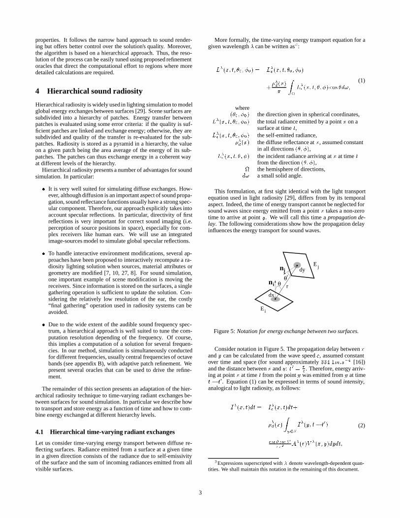
Figure 5: Notation for energy exchange between two surfaces.

Consider notation in Figure 5. The propagation delay between xand y can be calculated from the wave speed c, assumed constantover time and space (for sound approximately 334:1m:s

�1 [16])and the distance between x and y: t 0 = r

c. Therefore, energy arriv-

ing at point x at time t from the point y was emitted from y at timet � t

0. Equation (1) can be expressed in terms of sound intensity,analogical to light radiosity, as follows:

I�(x; t)dt = I

�

e (x; t)dt+

��

d(x)

Zy2S

I�(y; t� t

0)

cos � cos �0

�r2A�(r)V �(x; y)dydt;

(2)

3Expressions superscripted with � denote wavelength-dependent quan-tities. We shall maintain this notation in the remaining of this document.

3

where (see also notations in Figure 5)I�(x; t)dt the total energy emitted from the point x at time t

during a short emission time dt,I�

e (x; t)dt the self-emitted energy during dt,I�(y; t � t

0) the energy emitted from the point y at time t� t0,

A�(r) a medium scattering coefficient,

V�(x; y) a ¡¡visibility¿¿ term due to diffraction by

occluders [33, 34],S a set of surfaces in the scene.

The expression under integral in equation (2) describes the inten-sity contribution from any point y for which the propagation delayto the point x is equal to t

0. Taking the integral of this term overall surfaces S in the scene gives the total intensity that arrives at xat time t. This integral can be rewritten by sorting the points y bytheir propagation delay to x:

Z1

�=0

Zy2S�

I�(y; t � �)F�(x; y)dyd�; (3)

where� the propagation delay between x and y,

S� the set of points y with the propagation delay to xequal to � ,

F�(x; y) a point-to-point “form factor” between x and y.

Let us consider now that surfaces are discretized into a set ofpolygonal patchesPi. We assume that the intensity is spatially con-stant over a patch and during the exchange:

I�

i (x; t) � I�

i Ie�

i (x; t) � Ie�

i :

Surfaces are of finite extend, we must take into account a durationof the exchange defined as the difference between the maximum�max and the minimum �min propagation delays between points ona pair of patches.

We can thus rewrite equation 3 as:

Ii(t) = Iei(t)+

= I�

j (t� Tij)

Z�max

�min

Zy2Pj

F�

ij(x; y)�(r � c�)dyd�

| {z }F�

ij(�)

;

(4)

where Tij = �min is the minimum propagation delay between thetwo patches, �(r � c�) is a Dirac distribution which is non zeroonly for pairs of points such as the propagation delay is equal to �and F �

ij(�) is the geometric form factor betweenPi and Pj .

Thus, we can derive a discrete version of equation (4):

E�

i [t] = Ee

�

i [t] + ��

i

NXj=1

F�

ijI�

j [t� Tij ]; (5)

where square brackets indicate that the energy iscalculated only for some discrete values of time,

E�

i [t] the total energy emitted by patch Pi at time t,Ee

�

i [t] the energy self-emitted by patch Pi at t,��

i the diffuse reflectance of patch Pi (constant),F�

ij the form factor between patchesPi and Pj ,Tij is the minimum propagation delay between between Pi and Pj ,

I�

j [t� Tij ] the intensity emitted by Pj at time t� Tij .

Equation (5) describes time-varying energy exchanges betweentwo patchesPi and Pj.

The three principal components of a time-varying energy ex-change are then:

� A wavelength-dependent form factor F �

ij defined by:

F�

ij =1

Ai

Zx2Pi

Zy2Pj

cos � cos �0

�r2A�(r)V (x;y)dxdy

computed as an average of point-to-polygon form factors forsampled points on Pj. Note that the visibility term is nolonger marked as wavelength-dependent. Indeed, during theform factor calculation, additional evaluation of a frequencydependent visibility term would be too expensive. The effectsof diffraction are most noticeable for direct sound which hasnot hit a surface at the time of form factor calculation. Thus,we assume the visibility to be standard light, geometric vis-ibility and compute a diffraction term for direct sound onlyusing an approach similar to [33, 34].

Point to polygon form factors are also computed by sam-pling the receiving patch Pi. Taking the following def-inition for a point-to-point delta form factor �F �

cos � cos �0

�r2A�(r)V (xn; ym) we obtain:

F�

ij =1

Ai

NXn=1

MXm=1

�Fdxndym (6)

� The minimum propagation delay Tij computed for all couplesof visible sample points on patch Pi and Pj :

Tij = minx2Pi ;y2Pj

r

c; (7)

where r is the distance between x and y, mutually visiblepoints respectively on Pi and Pj .

� The duration of the exchange �ij defined by:

�ij = maxx2Pi ;y2Pj

r

c� min

x2Pi ;y2Pj

r

c: (8)

Two linked patches exchange energy in an iterative process, eachiteration corresponding to an order of reflection. At each iterationoracles are used to evaluate the quality of the energy transfer. Ifquality constraints are not met, patches are subdivided and linksare refined. The process is iterated until it reaches a given orderof reflection or until overall energy gathered by all surfaces has de-cayed by more that 60 dB relative to the energy originally sent bythe source (which is the criterion commonly used in room acousticsto measure the duration of the reverberation).

4.2 Echos: representing sound intensity through time

∆

T

Echot

IEchogramme

t

I

Figure 6: Representing sound intensity through time.

Equation 5 provides a discrete space/time formulation for time-varying radiant exchanges. An elementary information that is going

4

to be exchanged between patches is an “echo”. It can be seen as anenergy distribution during a time interval corresponding to the du-ration of the exchange and modified by each reflection. An echoarriving on a patch is thus described by three quantities (Figure 6):

� an arrival time, T

� an intensity, I

� a width, �

+

+∆

τ

T

T

I

τ

F

I.F

Αj

Αi

∆

j

ij

ij

E i

ij

Αi

Αj

i

Τ j

Ej

ijΤ

i

Figure 7: The temporal energy transport operator. A i and Aj arethe areas of patches Pi and Pj.

At the beginning of the process punctual sound sources emit asingle Dirac echo of unit energy and zero width. These echos arethen propagated from patch to patch using the transport operator,defined in equation (5) and graphically illustrated in Figure 7. Eachreflection modifies the echo: the energy of the received echo be-comes equal to the energy of the shot echo multiplied by the formfactor; its arrival time is augmented by a patch-to-patch propagationdelay; and its width is extended by the exchange duration.

Equation (5) defines discrete energy exchanges between sur-faces. In order to represent the energy received/emitted by a surfacethrough time, we store a list of echos on each patch in echogramsas presented in section 2.1. Each patch stores relevant informationin three echograms:

� a shooting echogram which stores echos to be shot during thecurrent iteration,

� a gathering echogram in which gathered echos will be storedbefore the “push-pull”, and

� an overall echogram storing all echos gathered through timeby the patch at its level in the hierarchy only. Note that theenergy is not stored in a pyramid to avoid memory overhead.

As in standard hierarchical radiosity algorithms, energy receivedby a father patch must be “pushed” to its children and then “pulled”to shoot coherent values of energy during the next iteration. Thisprocess is similar to the classic “push-pull” process of hierarchi-cal light radiosity. However, due to the temporal nature of theexchange, one extra detail must be taken into account. When anecho has been received by a father patch, its propagation time hasto be corrected before it can be reshot by the children to take intoaccount the difference in propagation time between the shooter-to-father path and the shooter-to-child path (T1 and T2 in Figure 8).

In order to compute this correction, each echo stores a value iden-tifying its shooter. Then, an approximate correction is computedby evaluating the difference between propagation time from theshooter patch to children patches centroids and to the father patchcentroid. A similar time correction must be used when refining ashooting patch. The correction can be performed at the moment ofthe shooting/gathering operation.

Τ1

Τ2

Figure 8: Handling hierarchical propagation delays. Energy re-ceived at time T1 by a patch should not be reshot at time T1 fromits children. A time correctionT2� T1 is added before reshootingthe echo from the children.

In order to accelerate all inserting/deleting echos operations,echograms are structured as binary trees of echoes, sorted by theirarrival time on the patch.

4.3 Space-frequency refinement

We propose to use two oracles to control the spatial subdivisionof surfaces in the scene. Since they depend on data that is itselfwavelength-dependent (e.g. form factors), they lead to differentsubdivisions at different frequencies.

� A standard BF� oracle which refines patches that receive thehighest energy.

� A consistency oracle T� that guarantees that the hypothesison the surfaces shooting energy in phase is valid (and so is theenergetic formulation). It chooses for refinement the patchesfor which the exchange duration is high. Figure 9 shows anexample of such a subdivision for different frequency bands.The subdividing criterion is:

�ij > T�c

�

Note that at high frequencies, this oracle tends to be ineffec-tive, calling for the use of time corrections as presented in theprevious section.

4.4 Echo Fusions

In order to handle the overwhelming number of echoes and be ableto simulate quickly higher orders of reflection we designed an echomerging mechanism such that several echoes can be combined in anew one. The main problem in merging echos together is to guar-antee that possible interferences are taken into account in order notto over estimate the energy. Two cases of echo merging can occur:coherent echos and incoherent echos merging.

Coherent echo merging occurs when two (or more) echos reacha surface coming from the same shooter with an arrival time dif-ference a priori inferior from the period T = c=� of the signal.In this case we can reconstruct the two complex pressure distribu-tions associated with each echo and sum them up to get a new echo.

5

(a) (b)

Figure 9: Example of frequency refinement on T � oracle at (a) 50Hz, (b) 100 Hz. Value of the oracle is 1.0

+I

∆ ∆2

I

+(∆ + ∆ )1 2

2

1

= I1

t

t - t

11 t2 t +dt

1 2

Figure 10: Summing echos together

Each echo represents a complex pressure distribution through timeP = Ee

i!t; where E is the square root of the intensity of the echo

4. We can thus write:

P1 = E1ei!t1

; P2 = E2ei!t2

;

where ! = 2�c�

and

P1 + P2 = P1(1 +P2

P1) = Ee

(!(t1+dt));

where

E =pE1

2 + E22 + E1E2 cos (!(t2 � t1))

and

dt =1

!atan(

E2 sin (!(t2 � t1))

E1 +E2 cos (!(t2 � t1))):

We use a parameter m to merge coherent echoes that reach a sur-face within a time-step defined by � = mT . Effects of coherentecho merging efficiency and energy conservation are illustrated onfigures 11 and 12.

4.5 Handling specular reflections

Surface reflectances for sound usually have a strong specular com-ponent. Thus, in order to be able to simulate this essential specularterm we propose to extend our method to take into account com-bined ideal specular and ideal diffuse reflectors. To achieve thisgoal, we use an image-source like approach. We extend the datastructure used to represent the echos in order to store a point of ori-gin. When echos are gathered from a specular surface, we use thisorigin point to construct a mirrored image according to the planeof the shooting patch (see Figure 13). A point-to-element extended

4 intensity is proportional to the mean square pressure over time:I = p2=�0c where �0c is the characteristic impedance of the medium(414kg:m�2:s�1 for air)

facteur de fusion

0

0

0

0

20%

temps (s)

Intensité (dB)

10%

0%

100%

0.01 0.02

100

100

100

100

0.03 0.080.070.060.050.04

Figure 11: Comparison of four echograms resulting from simula-tions with different coherent echo merging factors. Note that theenergy does not tend to be overestimated by the merging process.

pas de fusion

500%

20%

2%

0%

Figure 12: Comparison of the number of echoes function of theorder of reflection for different values of the coherent echo mergingthresholdm. From 0% (top curve) to 500% (bottom curve).

form factor is computed and a new echo is transfered to the gather-ing patch. To simplify the process, when echos come from surfacicelements we use the centroid of the element as the point of origin.This operation is similar to a “three-point transport”. Of course ifthe specular reflector also has a diffuse component, a “standard”echo is also exchange using the extended form factor between thesource and gathering patch. This approach allows to maintain spe-cial echos which have zero duration and represent pure specularpaths of reflection, which are very important since they will be re-sponsible for the strongest reflections. We do not store in that casethe intensity of the echo but the product of all reflection coefficientsalong the path. Since we also store the propagation time we canthus re-compute the intensity emitted by the equivalent point soundsource.

This source-image approach is conducted with each element. Ifelements are sub-patches of the same surface, several copies of thesame source-image will be generated in the case of pure specularpaths. We can however eliminate those duplicates when performingthe push-pull operation by specifying that echos of zero durationand same origin point can be merged together.

5 Implementating the approach

As in common hierarchical radiosity approaches, there are basicallytwo ways of implementating the process. The approach we choseis to refine using the energetic oracle. Since the energy is decreas-ing with time, resolution of the process gets more and more coarse.This allows us to get fine results for beginning times of the sim-ulation and more coarse, but fast ones for the late reverberation.Implementation using this approach is also very straightforward.

6

E

E

(b)

E

S’

E 3

2

1

2 E

E1

3

(a)

Figure 13: Using the center of the element to build an image-sourcefor specular exchanges. The center of the origin element E 1 of theecho is mirrored according to the source element E 2 . An extendedform factor is then computed between the obtained point (S') andthe receiving element E3 .

Moreover, since it is very time consuming to perform the push-pull operation on every element, we propose to maintain an integralvalue of all the intensity that has been exchanges during the timeof one iteration. This value is computed as the sum of the energiesof the echos for each echogram. We perform a standard push-pulloperation on those values and use them to evaluate the refinementoracles. When the appropriate level of exchange has been selected,the push-pull operation is performed on the shooting echograms ofthe shooter's hierarchy.

However, the major drawback is that the refinement operatordoes not use a global estimate of the solution. Another possibil-ity is then to perform a complete simulation until convergence us-ing links of highest level in the hierarchy. The obtained solution isthen coarse but covers the complete duration of the simulation. If arefinement operation is performed at this time, the oracle can bet-ter estimate the links through which energy has most transited overtime. But the drawback then is that all the echoes that were trans-mitted through the old links must be canceled before being reshotthrough the new ones. Once again, the cancellation operation canbe quite costly since it involves to reshoot each echo with a negativeintensity value.

6 Application to acoustic simulations anddata visualization

In this section we present examples of acoustic simulations andacoustic data visualization aimed at validating our simulation tech-nique in the case of concert hall design applications. A few ap-proaches have already been presented to visualize acoustic data [31,24]. They are based on ray-tracing techniques which seems lesssuitable for visualization since no direct information is available onsurfaces. Thus sampling of the surfaces must be done as a postpro-cessing [24]. In our approach, since surfaces are discretized for theradiosity process, visualization of relevant acoustic data can be eas-ily integrated in the simulation. By displaying energy that transitedon the links designer can easily check for problems in the hall de-sign (lack of lateral energy for example) (see figure 14). Once thetime-varying radiosity solution is computed, an animated render-ing of energy reaching surfaces through time can also be displayedin real-time to analyze the wave front propagation (see figure 16).Figures 14 and 15 present other examples of visualization in anacoustic simulation context.

(a)

(b)

(c)

Figure 14: Visualization of acoustic simulation data. Sound sourceis displayed as yellow spheres, microphones as blue ones. Figure(a) and (b) show overall energy received by the surfaces throughtime. (c) is a display of the overall energy that transited throughlinks reaching the microphone. This kind of visualization may allowthe designer to detect problems related with spatial distribution ofthe energy.

7 Conclusion

We presented a new solution to acoustic simulations based on a ra-diant exchange approach adapted to take into account time-varyingphenomena. This approach is well suited to simulate global dif-fuse reflections and has been modified to handle specular reflectionswhich are of primary importance for sound. Moreover, we pre-sented an extension that allows for tuning the temporal complexityof the process while taking into account interferences. The result-ing solution is stored on the surfaces of the environment. Thus, itis quasi listener-independent. Only a final gathering step is neededwhen the receiving point is moving, which offers the possibility touse this method for interactive walkthroughs. The solution also pro-vide interesting ways of visualizing spatial and time-varying phe-nomena.

Of course, many points could be improved in our method. Exten-sions include further acoustic validation of the method. Taking intoaccount a “phase” factor in the form factors could significantly im-

7

Figure 15: Visualization of acoustic simulation data in the Operade la Bastille in Paris and in another smaller hall.

prove the solution if patches large compared to the wavelength areused. We are also thinking of extending the hierarchical approachto take into account clusters of surfaces and perform incrementalupdate of the solution. We could also think of separating the calcu-lation of the images-sources of the energy exchange process. Sincewe recompute the image-sources each time we exchange the echos,we should improve a lot the efficiency of our approach.

A Surface reflectance for sound

Usually, wide band data of complex material absorption filters arenot available, due to the difficulty of the measurements. In practicethe most common coefficients are Sabine's diffuse field absorptioncoefficients �� given in octave bands. Thus, reflected energy co-efficient is (1 � �

�). Another coefficient �� defines the propor-tion of energy which is diffusely reflected. Thus diffuse reflectioncoefficient is (1 � �

�)�� and the specular reflection coefficient is(1��

�)(1���). Below, we present a few examples of reflectance

coefficients measured in a real concert hall. Note the high diffusionaspect of some materials:

Material 125 Hz 250 Hz 500 Hz 1 kHz 2 kHz 4 kHzAudience (seats) 0.30 0.45 0.50 0.60 0.65 0.70Back wall (carpet) 0.10 0.10 0.10 0.09 0.09 0.07Ceiling (stucco) 0.25 0.30 0.30 0.35 0.35 0.40Stage (parquet floor) 0.05 0.05 0.04 0.03 0.01 0.01

Figure 16: Visualization of a wavefront propagation with one orderof reflection by displaying our radiosity solution through time. Notethe two secondary wavefronts due to pure specular reflections onwalls on the second and third picture. The radiosity solutions wereobtained with 685 elements and 132610 links for the two faces and8193 elements/6188 links for the cube.

B Digital signal processing issues

Reconstructing the pressure impulse response

Remember that our simulation process is a narrow band approach.At the end of the simulation our solution consists of severalechograms for different octave bands. Reconstructing the pressureimpulse response involves three steps:

� For each echogram, reconstruct the pressure data stored ineach echo to obtain a one wide band pressure impulse re-sponse. Retrieving the wide band pressure information storedin an echo can be achieved simply by replacing the echo by agiven time “window function” defined on the width � of theecho and whose integral on this time-step is the square rootof the energy of the echo (remember that the energy is pro-portional to the square root of the pressure). In our currentimplementation, we use a window function f� defined by:

f�(x) = 1� sin (2�x

�);

for x 2 [��; �]:

The pressure impulse response is then given by:

P (t) =Xi

p(Ei)

�if�i(t� ti)

� Filter the obtained wide band pressure impulse responses bythe corresponding band pass filter to keep only the valid partof the response (remember that all values in echos were com-puted for a specific frequency band).

8

� Add the obtained “narrow band” pressure impulse responsestogether to get the final wide band pressure impulse responseof the environment.

∗

∗

∗

+

Figure 17: Converting echograms in octave bands to a pressureimpulse response.

References[1] J.B. Allen and D.A. Berkley. Image method for efficiently simulating small room

acoustics. Journal of the Acoustical Society of America, 65(4), 1979.

[2] D.R. Begault. Challenges to the successful implementationof 3D sound. Journalof the Audio Engineering Society, 39(11):864–870, November 1991.

[3] Durand R. Begault. 3D Sound for Virtual Reality and Multimedia. AcademicPress Professional, 1994.

[4] J. Blauert. Spatial Hearing : The Psychophysics of Human Sound Localization.M.I.T. Press, Cambridge, MA, 1983.

[5] J. Borish. Extension of the image model to arbitrary polyhedra. Journal of theAcoustical Society of America, 75(6), 1984.

[6] D.A. Burgess. Real-time audio spatialization with inexpensive hardware. Tech-nical Report GIT-GVU-92-20, Georgia Institute of Technology, 1992.

[7] Shenchang E. Chen. Incremental radiosity: an extension of progressive radios-ity to an interactive image synthesis system. ACM Computer Graphics, SIG-GRAPH'90 Proceedings, 24(4):135–144, August 1990.

[8] G. Drettakis and F.X. Sillion. Interactive update of global illumination usinga line-space hierarchy. ACM Computer Graphics, SIGGRAPH'97 Proceedings,pages 57–64, August 1997.

[9] S.H. Foster, E.M. Wenzel, and R.M. Taylor. Real-time synthesis of complexenvironments. Proc. of the ASSP (IEEE) Workshop on Application of SignalProcessing to Audio and Acoustics, 1991.

[10] D.W. George, F.X. Sillion, and D.P. Greenberg. Radiosity redistribution for dy-namic environments. IEEE Computer Graphics and Applications, pages 26–34,July 1990.

[11] C.H. Haan and F.R. Fricke. An evaluation of the importanceof surface diffusivityin concert halls. Applied Acoustics, 51(1):53–69, 1997.

[12] R. Heinz. Binaural room simulation based on an image source model with addi-tion of statistical methods to include the diffuse sound scattering of walls and topredict the reverberant tail. Applied Acoustics, 38:145–159, 1993.

[13] M. Kleiner, B.I. Dalenbak, and P. Svensson. Auralization - an overview. Journalof the Audio Engineering Society, 41(11):861–875, November 1993.

[14] M. Kleiner, R. Orlowski, and J. Kirszenstein. A comparison between resultsfrom a physical scale model and a computer image source model for architecturalacoustics. Applied Acoustics, 38:245–265, 1993.

[15] H. Kuttruff. On the audibility of phase distorsions in rooms and its significancefor sound reproducitonand digital simulation in room acoustics. Acustica, 74(1),1991.

[16] Heinrich Kuttruff. Room Acoustics (3rd edition). Elseiver Applied Science,1991.

[17] K.H. Kuttruff. Auralization of impulse responses modeled on the basis of ray-tracing results. Journal of the Audio Engineering Society, 41(11):876–880,November 1993.

[18] Y.W. Lam. The dependance of diffusion parameters in a room acoustics predic-tion model on auditorium sizes and shapes. Journal of the Acoustical Society ofAmerica, 100(4):2193–2203, October 1996.

[19] H. Lehnert. Systematic errors of the ray-tracing algorithm. Applied Acoustics,38, 1993.

[20] H. Lehnert and J. Blauert. Principles of binaural room simulation. AppliedAcoustics, 36:259–291, 1992.

[21] T. Lewers. A combined beam tracing and radiant exchange computer model ofroom acoustics. Applied Acoustics, 38, 1993.

[22] J. Martin, D. van Maercke, and J.P. Vian. Binaural simulation of concert halls :A new approach for the binaural reverberationprocess. Journal of the AcousticalSociety of America, 94:3255–3263, December 1993.

[23] Henrik Møller. Fundamentals of binaural technology. Applied Acoustics,36:171–218, 1992.

[24] M. Monks, B.M. Oh, and J. Dorsey. Acoustic simulation and visualisation usinga new unified beam tracing and image source approach. Proc. Audio EngineeringSociety Convention, 1996.

[25] J.A. Moorer. About this reverberationbusiness. Computer Music Journal, 23(2),1979.

[26] J.M. Naylor. Odeon - another hybrid room acoustical model. Applied Acoustics,38(1):131–143, 1993.

[27] J. Nimeroff, J. Dorsey, and H. Rushmeier. Implementation and analysis of animage-based global illumination framework for animated environments. IEEETransactions on Visualization and Computer Graphics, 2(4), December 1996.

[28] J.D. Polack. Playing billiards in the concert hall: The mathematical foundationsof geometrical room acoustics. Applied Acoustics, 38:235–244, 1993.

[29] Francois X. Sillion and C. Puech. Radiosity and Global Illumination. MorganKaufmann Publishers inc., 1994.

[30] F.X. Sillion and C. Puech. A general two pass method integrating specular anddiffuse reflection. ACM Computer Graphics, SIGGRAPH'89Proceedings, 23(3),July 1989.

[31] Adam Stettner and Donald P. Greenberg. Computer graphics visualisation foracoustic simulation. ACM Computer Graphics, SIGGRAPH'89 Proceedings,23(3):195–206, July 1989.

[32] Tapio Takala and James Hahn. Sound rendering. ACM Computer Graphics,SIGGRAPH'92 Proceedings, 28(2), July 1992.

[33] Nicolas Tsingos and Jean-Dominique Gascuel. Soundtracks for computer an-imation: sound rendering in dynamic environments with occlusions. Proc. ofGraphics Interface'97, 1997.

[34] Nicolas Tsingos and Jean-Dominique Gascuel. Fast rendering of sound occlu-sion and diffraction effects for virtual acoustic environments. Proc. 104th AudioEngineering Society Convention, May 1998.

[35] D. van Maercke and J. Martin. The prediction of echograms and impulse re-sponses within the Epidaure software. Applied Acoustics, 38(1):93–114, 1993.

[36] E.M. Wenzel and S.H. Foster. Realtime digital synthesis of virtual acoustic envi-ronments. Computer Graphics (Proc. ACM Symposium on Interactive 3D Com-puter Graphics), 24(2):139–140, March 1990.

9