acta universitatis upsaliensis uppsala dissertations from ... · acta universitatis upsaliensis...
TRANSCRIPT

ACTA UNIVERSITATIS UPSALIENSISUppsala Dissertations from the Faculty of Science and Technology
66


Milena Ivanova
Scalable Scientific Stream QueryProcessing

Dissertation at Uppsala University to be publicly examined in MIC campus, room 1211, Po-lacksbacken, on Monday, November 7, 2005 at 13:15, for the Degree of Doctor of Philosophy.The examination will be conducted in English.
AbstractIvanova, M. 2005. Scalable Scientific Stream Query Processing. Acta Universitatis Upsaliensis.Uppsala Dissertations from the Faculty of Science and Technology 66. 137 pp. Uppsala. ISBN91-554-6351-7
Scientific applications require processing of high-volume on-line streams of numerical datafrom instruments and simulations. In order to extract information and detect interesting pat-terns in these streams scientists need to perform on-line analyses including advanced and of-ten expensive numerical computations. We present an extensible data stream management sys-tem, GSDM (Grid Stream Data Manager) that supports scalable and flexible continuous queries(CQs) on such streams. Application dependent streams and query functions are defined throughan object-relational model.
Distributed execution plans for continuous queries are specified as high-level data flow dis-tribution templates. A built-in template library provides several common distribution patternsfrom which complex distribution patterns are constructed. Using a generic template we de-fine two customizable partitioning strategies for scalable parallel execution of expensive streamqueries: window split and window distribute. Window split provides parallel execution of ex-pensive query functions by reducing the size of stream data units using application dependentfunctions as parameters. By contrast, window distribute provides customized distribution of en-tire data units without reducing their size. We evaluate these strategies for a typical high volumescientific stream application and show that window split is favorable when expensive queriesare executed on limited resources, while window distribution is better otherwise. Profile-basedoptimization automatically generates optimized plans for a class of expensive query functions.We further investigate requirements for GSDM in Grid environments.
GSDM is a fully functional system for parallel processing of continuous stream queries.GSDM includes components such as a continuous query engine based on a data-driven data flowparadigm, a compiler of CQ specifications into distributed execution plans, stream interfacesand communication primitives. Our experiments with real scientific streams on a shared-nothingarchitecture show the importance of both efficient processing and communication for efficientand scalable distributed stream processing.
Keywords: data stream management systems, parallel stream processing, scientific stream queryprocessing, user-defined stream partitioning
Milena Ivanova, Department of Information Technology, Uppsala University, PO-Box 337, SE-751 05 Uppsala, Sweden
c©Milena Ivanova 2005
ISSN 1104-2516ISBN 91-554-6351-7
Printed in Sweden by Universitetstryckeriet, Uppsala 2005Distributor: Uppsala University Library, Box 510, SE-751 20 Uppsalawww.uu.se, [email protected]

To my parents andmy son


Contents
1 Introduction . . . . . . . . . . . . . . . . . . . . . . . . . . . . . . . . . . . . . . . . . . 11.1 Motivation . . . . . . . . . . . . . . . . . . . . . . . . . . . . . . . . . . . . . . . . 11.2 Database Management Systems . . . . . . . . . . . . . . . . . . . . . . . . 21.3 Distributed and Parallel DBMS . . . . . . . . . . . . . . . . . . . . . . . . 5
1.3.1 Parallel Database Architectures . . . . . . . . . . . . . . . . . . . . 61.3.2 Types of Parallelism for DBMS . . . . . . . . . . . . . . . . . . . . 7
1.4 Data Stream Management Systems (DSMSs) . . . . . . . . . . . . . . 81.5 Summary of Contributions and Thesis Outline . . . . . . . . . . . . . 11
2 GSDM System Architecture . . . . . . . . . . . . . . . . . . . . . . . . . . . . . . 152.1 Scenario . . . . . . . . . . . . . . . . . . . . . . . . . . . . . . . . . . . . . . . . . 152.2 Query Specification and Execution . . . . . . . . . . . . . . . . . . . . . 162.3 GSDM Coordinator . . . . . . . . . . . . . . . . . . . . . . . . . . . . . . . . . 192.4 GSDM Working Nodes . . . . . . . . . . . . . . . . . . . . . . . . . . . . . . 212.5 CQ Life Cycle . . . . . . . . . . . . . . . . . . . . . . . . . . . . . . . . . . . . . 23
2.5.1 Compilation . . . . . . . . . . . . . . . . . . . . . . . . . . . . . . . . . . 242.5.2 Execution . . . . . . . . . . . . . . . . . . . . . . . . . . . . . . . . . . . . 242.5.3 Deactivation . . . . . . . . . . . . . . . . . . . . . . . . . . . . . . . . . . 26
3 An Object-Relational Stream Data Model and Query Language . . . 273.1 Amos II Data Model and Query Language . . . . . . . . . . . . . . . . 273.2 Stream Data Model . . . . . . . . . . . . . . . . . . . . . . . . . . . . . . . . . 28
3.2.1 Window Functions . . . . . . . . . . . . . . . . . . . . . . . . . . . . . . 293.2.2 Stream Types . . . . . . . . . . . . . . . . . . . . . . . . . . . . . . . . . . 303.2.3 Registering Stream Interfaces . . . . . . . . . . . . . . . . . . . . . 32
3.3 Query Language . . . . . . . . . . . . . . . . . . . . . . . . . . . . . . . . . . . 323.3.1 Defining Stream Query Functions . . . . . . . . . . . . . . . . . . 333.3.2 SQF Discussion . . . . . . . . . . . . . . . . . . . . . . . . . . . . . . . . 333.3.3 Transforming SQFs . . . . . . . . . . . . . . . . . . . . . . . . . . . . . 343.3.4 Combining SQFs . . . . . . . . . . . . . . . . . . . . . . . . . . . . . . . 36
3.4 Data Flow Distribution Templates . . . . . . . . . . . . . . . . . . . . . . 373.4.1 Central Execution . . . . . . . . . . . . . . . . . . . . . . . . . . . . . . 373.4.2 Partitioning . . . . . . . . . . . . . . . . . . . . . . . . . . . . . . . . . . . 383.4.3 Parallel Execution . . . . . . . . . . . . . . . . . . . . . . . . . . . . . . 393.4.4 Pipelined Execution . . . . . . . . . . . . . . . . . . . . . . . . . . . . . 403.4.5 Partition-Compute-Combine (PCC) . . . . . . . . . . . . . . . . . 40
vii

3.4.6 Compositions of Data Flow Graphs . . . . . . . . . . . . . . . . . 414 Scalable Execution Strategies for Expensive CQ . . . . . . . . . . . . . . 43
4.1 Window Split and Window Distribute . . . . . . . . . . . . . . . . . . . 434.2 Parallel Strategies Implementation in GSDM . . . . . . . . . . . . . . 45
4.2.1 Window Split Implementation . . . . . . . . . . . . . . . . . . . . . 464.2.2 Window Distribute Implementation . . . . . . . . . . . . . . . . . 49
4.3 Experimental Results . . . . . . . . . . . . . . . . . . . . . . . . . . . . . . . . 504.3.1 Performance Metrics . . . . . . . . . . . . . . . . . . . . . . . . . . . . 504.3.2 FFT Experiments . . . . . . . . . . . . . . . . . . . . . . . . . . . . . . . 514.3.3 Analysis . . . . . . . . . . . . . . . . . . . . . . . . . . . . . . . . . . . . . 58
5 Definition and Management of Continuous Queries . . . . . . . . . . . . 615.1 Meta-data for CQs . . . . . . . . . . . . . . . . . . . . . . . . . . . . . . . . . . 615.2 Data Flow Graph Definition . . . . . . . . . . . . . . . . . . . . . . . . . . . 635.3 Templates Implementation . . . . . . . . . . . . . . . . . . . . . . . . . . . . 64
5.3.1 Central Execution . . . . . . . . . . . . . . . . . . . . . . . . . . . . . . 655.3.2 Partitioning . . . . . . . . . . . . . . . . . . . . . . . . . . . . . . . . . . . 655.3.3 Parallel execution . . . . . . . . . . . . . . . . . . . . . . . . . . . . . . 665.3.4 Pipelined execution . . . . . . . . . . . . . . . . . . . . . . . . . . . . . 67
5.4 CQ Management . . . . . . . . . . . . . . . . . . . . . . . . . . . . . . . . . . . 685.4.1 CQ Compilation . . . . . . . . . . . . . . . . . . . . . . . . . . . . . . . 685.4.2 Mapping . . . . . . . . . . . . . . . . . . . . . . . . . . . . . . . . . . . . . 735.4.3 Installation . . . . . . . . . . . . . . . . . . . . . . . . . . . . . . . . . . . 735.4.4 Activation . . . . . . . . . . . . . . . . . . . . . . . . . . . . . . . . . . . . 745.4.5 Deactivation . . . . . . . . . . . . . . . . . . . . . . . . . . . . . . . . . . 74
5.5 Monitoring Continuous Query Execution . . . . . . . . . . . . . . . . . 755.6 Data Flow Optimization . . . . . . . . . . . . . . . . . . . . . . . . . . . . . 76
5.6.1 Estimating Plan Costs . . . . . . . . . . . . . . . . . . . . . . . . . . . 765.6.2 Plan Enumeration . . . . . . . . . . . . . . . . . . . . . . . . . . . . . . 76
6 Execution of Continuous Queries . . . . . . . . . . . . . . . . . . . . . . . . . . 796.1 SQF Execution . . . . . . . . . . . . . . . . . . . . . . . . . . . . . . . . . . . . 79
6.1.1 Operator Structure . . . . . . . . . . . . . . . . . . . . . . . . . . . . . . 796.1.2 Execute operator . . . . . . . . . . . . . . . . . . . . . . . . . . . . . . . 816.1.3 Implementation of S-Merge SQF . . . . . . . . . . . . . . . . . . . 826.1.4 Implementation of OS-Join SQF . . . . . . . . . . . . . . . . . . . 83
6.2 Inter-GSDM communication . . . . . . . . . . . . . . . . . . . . . . . . . . 856.3 Scheduling . . . . . . . . . . . . . . . . . . . . . . . . . . . . . . . . . . . . . . . 86
6.3.1 Scheduling periods . . . . . . . . . . . . . . . . . . . . . . . . . . . . . 866.3.2 SQF Scheduling . . . . . . . . . . . . . . . . . . . . . . . . . . . . . . . 876.3.3 Scheduling of System Tasks . . . . . . . . . . . . . . . . . . . . . . . 886.3.4 Effects of scheduling on system performance . . . . . . . . . . 88
6.4 Activation and Deactivation . . . . . . . . . . . . . . . . . . . . . . . . . . . 926.5 Impact of Marshaling . . . . . . . . . . . . . . . . . . . . . . . . . . . . . . . 92
viii

7 Continuous Queries in a Computational Grid Environment . . . . . . . 957.1 Overview of Grids . . . . . . . . . . . . . . . . . . . . . . . . . . . . . . . . . . 957.2 Integrating Databases and Grid . . . . . . . . . . . . . . . . . . . . . . . . 967.3 GSDM as an Application for Computational Grids . . . . . . . . . 96
7.3.1 GSDM Requirements for Grids . . . . . . . . . . . . . . . . . . . . 977.3.2 GSDM Resource Allocation . . . . . . . . . . . . . . . . . . . . . . 987.3.3 Multiple Grid Resources . . . . . . . . . . . . . . . . . . . . . . . . . 997.3.4 Grid Requirements for Applications . . . . . . . . . . . . . . . . . 99
7.4 Related Projects on Grid . . . . . . . . . . . . . . . . . . . . . . . . . . . . . 1007.4.1 OGSA-DAI . . . . . . . . . . . . . . . . . . . . . . . . . . . . . . . . . . . 1007.4.2 OGSA-DQP . . . . . . . . . . . . . . . . . . . . . . . . . . . . . . . . . . 1007.4.3 GATES . . . . . . . . . . . . . . . . . . . . . . . . . . . . . . . . . . . . . . 1027.4.4 R-GMA . . . . . . . . . . . . . . . . . . . . . . . . . . . . . . . . . . . . . . 103
8 Related work . . . . . . . . . . . . . . . . . . . . . . . . . . . . . . . . . . . . . . . . . 1058.1 Data Stream Management Systems . . . . . . . . . . . . . . . . . . . . . 105
8.1.1 Aurora . . . . . . . . . . . . . . . . . . . . . . . . . . . . . . . . . . . . . . . 1068.1.2 Aurora*, Medusa, and Borealis . . . . . . . . . . . . . . . . . . . . 1078.1.3 Telegraph and TelegraphCQ . . . . . . . . . . . . . . . . . . . . . . . 1088.1.4 CAPE . . . . . . . . . . . . . . . . . . . . . . . . . . . . . . . . . . . . . . . 1108.1.5 Distributed Eddies . . . . . . . . . . . . . . . . . . . . . . . . . . . . . . 1118.1.6 Tribeca . . . . . . . . . . . . . . . . . . . . . . . . . . . . . . . . . . . . . . 1128.1.7 STREAM . . . . . . . . . . . . . . . . . . . . . . . . . . . . . . . . . . . . 1138.1.8 Gigascope . . . . . . . . . . . . . . . . . . . . . . . . . . . . . . . . . . . . 1148.1.9 StreamGlobe . . . . . . . . . . . . . . . . . . . . . . . . . . . . . . . . . . 1158.1.10 Sensor Networks . . . . . . . . . . . . . . . . . . . . . . . . . . . . . . . 116
8.2 Continuous Query Systems . . . . . . . . . . . . . . . . . . . . . . . . . . . 1178.3 Database Technology for Scientific Applications . . . . . . . . . . . 1178.4 Parallel DBMS . . . . . . . . . . . . . . . . . . . . . . . . . . . . . . . . . . . . 118
9 Conclusions and Future Work . . . . . . . . . . . . . . . . . . . . . . . . . . . . 121References . . . . . . . . . . . . . . . . . . . . . . . . . . . . . . . . . . . . . . . . . . . . . . 131
ix


1. Introduction
This Thesis presents the design, implementation and evaluation of Grid StreamDatabase Manager (GSDM), a prototype of an extensible stream databasesystem for scientific applications. The main motivation of the project is toprovide scalable execution of computationally expensive analyses over datastreams specified in a high-level query language. This chapter presents theproblem description and introduces background knowledge about the mainenabling technologies for the GSDM prototype: database management sys-tems (DBMSs), distributed and parallel DBMSs, and the evolving area of datastream management systems. At the end of the chapter, we summarize themain contributions of the Thesis and describe the Thesis organization.
1.1 MotivationScientific instruments, such as satellites, on-ground antennas, and simulators,generate very high volume of raw data often in form of streams [55, 82]. Sci-entists need to perform a wide range of analyses over these raw data streamsin order to explore information and detect interesting events. Complex analy-ses are presently carried out off-line on data stored on disk using hard-codedpredefined processing of the data. The off-line processing has a number ofdisadvantages that reduce the potential usage of the raw data. It creates largebacklogs of unanalyzed data that prevents timely analysis after interesting nat-ural events occurred. The high data volume produced by scientific instrumentscan also be too large to be stored and processed.
One of the driving forces behind the development of the GSDM prototypewere the requirements of scientific applications from LOFAR/LOIS projects[54, 55]. The goal of the LOFAR project [54] in the Netherlands is to con-struct a radio telescope to receive signals from space and process them entirelyin software. The LOIS (LOFAR Outrigger in Scandinavia, http://www.lois-space.net/) extends LOFAR with dedicated space radio/radar facilities and ITinfrastructure with up to a few thousand units. As a part of LOIS a scientificinstrument has been constructed that is a specialized three-poled antenna re-ceiving radio signals. The signals are transformed from analogous into digitalformat, filtered initially by hardware, and sent in real time to the registeredclients (receivers). At the receiver side there is need for a data stream process-
1

ing system that allows users, scientists in space physics, to detect interestingevents in these high-volume signals by on-line analyses that include advancedand often expensive numerical computations.
The presence of high volume data and several users who want to performsimilar analyses on the data suggest the use of database technology. Databasemanagement systems have proven their efficiency in managing large amountsof data, providing fast extraction of data of interest through declarative querylanguages, allowing for concurrent data access to multiple users, etc. How-ever, several specific characteristics of scientific stream data and applicationsmake them not fitting well in the current DBMSs.
This Thesis presents our efforts to bring the advantages of database tech-nology to the class of scientific stream applications by the design and imple-mentation of a data stream management system where users can express andefficiently execute expensive scientific computations as high-level declarativedatabase queries towards the stream data.
The following three sections present the key technologies used in this The-sis. We end the chapter with a summary of our contributions.
1.2 Database Management SystemsDatabase management systems(DBMSs) (e.g. [34]) are software systems thatallow for creating and managing large amounts of data. A database is a col-lection of data managed by a DBMS. The DBMSs i) allow users to create newdatabases and specify the logical structure of the data called schema; ii) allowusers to query and modify the data using an appropriate language, called aquery language or data manipulation language; iii) support secure storage oflarge amounts of data over long period of time; iv) provide concurrent accessof multiple users to data.
DBMSs utilize various data models, which are primitives used for describ-ing the structure of the information in the database, the schema. The evolutionof DBMSs follows the development of new data models.
The first commercial DBMSs appeared in the late 1960s evolving from thefile systems that were used as the main tool for data management until then.These database management systems utilized hierarchical and network datamodels that provided users with a view over data close to the physical datarepresentation and storage. These early data models and systems did not sup-port high-level query languages. In order to retrieve the required data, usershad to navigate through a graph or tree of data elements connected by point-ers. Thus, database programming required considerable effort and changes inthe physical representation of data required rewriting database applications.
The relational data model proposed by Codd [26] at the beginning of 1970s
2

influenced significantly the development of database technology. Accordingto this model, data is presented to the users in form of two-dimensional tablescalled relations. The relations have one or more named columns and data en-tries called rows, or tuples. The crossing points of columns and rows containdata values that can be of different atomic types, e.g. numbers or strings ofcharacters. The simplicity of this conceptual view of data, close to the tra-ditional non-electronic data representations, was one of the main reasons forthe popularity it gained especially for business applications. At the same time,data is internally organized in complex data structures that allow for efficientaccess and manipulation.
In contrast to the earlier data models, the relational model allows for ex-pressing queries in a very high-level query language which substantially in-creases the efficiency of database programming. The queries can be specifiedusing two main formalisms: the procedural relational algebra and the declar-ative relational calculus. Based on these formalisms a number of query lan-guages have been proposed, among which Structured Query Language (SQL)became the widely used standard. Instead of navigating through low-level datastructures as in the early DBMSs, the users declaratively specify in SQL whatdata to be retrieved. The SQL query processing module takes care to translatethe declarative query into an efficient execution plan specifying how data is re-trieved. The separation of the query languages from the low-level implemen-tation details provides another important feature: data independence. Two lev-els of data independence are distinguished: the ability to change the physicaldata organization without affecting the application programs is called physicaldata independence, while logical data independence insulates programs fromchanges to the logical database design.
By the 1990s the relational databases were commonly used in businessapplications. However, a number of applications from new domains, suchas science, computer-aided engineering, and multimedia put requirements tothe database technology that exposed the limitations of the relational model.Among these requirements is the need to represent more complex objects andnew types of data such as audio and video, and to define specific operationsover them. These applications became a driving force for the development ofa new generation of DBMSs based on the object-oriented (OO) data model.All concepts in the OO paradigm are presented by objects classified in classes.A class consists of a type and possibly functions or procedures, called meth-ods, which can be executed on objects of that class. The type system is verypowerful: starting from atomic types, such as integers and strings, the user canbuild new types by using type constructors for record structures, collectiontypes (sets, bags, arrays, etc.), and reference types. Record structures and col-lection operators can be applied repeatedly to construct even more complextypes. Objects are assumed to have an object identity (OID) that identifies an
3

object independently of its value. Classes are organized in a class hierarchy,i.e. it is possible to declare one class A to be a subclass of another class B. Inthat case class A inherits all the properties of class B. The subclass may alsohave additional properties, including methods, that may be either in additionor in place of methods of the superclass.
Typically, OODBMSs were implemented by extending some object-orientedprogramming language, e.g. C++, with database features such as persistentstorage, concurrency control, and recovery. The object-oriented data modelis more powerful than the relational one when modeling real-world complexobjects and may provide higher performance. However, early OODBMSs didnot provide declarative query languages. Queries were specified by a naviga-tion through a graph of objects where the arcs are defined by OIDs stored asattribute values of other objects.
During the last decade the development of both RDBMSs and OODBMSsfollowed a common goal, namely to combine in one system the declarativepower of the relational DBMSs with the modeling power of the object-orientedparadigm. In the world of relational DBMSs most of the major vendors ex-tended gradually their systems with object-oriented capabilities establishing inthis way the new generation of object-relational DBMSs. The object-relationalmodel includes the following main extensions of the relational model [34,80]:• Extensible base type system. New user-defined base data types (UDTs)
can be introduced together with user-defined functions, operators, and ag-gregates operating on values of these types;
• Support for complex types by type constructors for rows (records of val-ues), collections (sets, bags, lists, and arrays), and reference types;
• Special operations, methods, can be defined for, and applied to, values of auser-defined types;
• Types can be organized in a hierarchy with support for inheritance of prop-erties from super types to subtypes;
• Unique object identifiers that distinguish an object independently of theobject’s data values.Most of the object-oriented extensions above were included in the object-
relational standard SQL:1999 [58] and its next edition SQL:2003 [31].Simultaneously object-oriented DBMSs have been developing to incorpo-
rate declarative query languages as well in order to gain the advantages of therelational systems. The ODMG (Object Data Management Group) created astandard including Object Definition Language (ODL) and Object Query Lan-guage (OQL) [30]. OQL combines the high-level declarative programming ofSQL with the object-oriented programming paradigm. It is intended to be usedas an extension of some object-oriented host language, such as C++ or Java.
In this Thesis we utilize an object-relational model for modeling streams
4

with complex content. User-defined types represent both stream data sources,i.e. the scientific instruments, and numerical stream data produced by them.User-defined functions implement application-specific operations. Inheritanceamong UDTs allows for code re-use, and encapsulation provides for data inde-pendence of the application queries from the physical stream representations.
1.3 Distributed and Parallel DBMSThe architecture of a DBMS can be centralized or distributed. In centralizedsystems all the data is stored in a single repository and is managed by a singleDBMS. In distributed database systems [64] data is stored in multiple repos-itories and is managed by a set of cooperating homogeneous DBMSs. Thedistributed DBMSs provide improved performance and reliability at the priceof higher complexity. The distribution is manual and very often appears natu-rally as a consequence of distributed business activities, for example, a bankhas one or several branches in different cities and countries and it is conve-nient to store and process branch-related data locally instead of in a singlecentral database.
Parallel DBMSs [29] are a special kind of distributed database systems withtransparent data distribution usually in one location to achieve better perfor-mance through parallel execution of various operations. The development ofthe parallel databases is in response to demands of applications that query ex-tremely large databases or perform extremely large number of transactions persecond, which the centralized DBMSs cannot handle.
The efficiency of parallel systems is evaluated by their speedup and scaleup.The speedup measures the ability of a parallel system to run a given task inless time by increasing the degree of parallelism. The scaleup measures theability to process larger tasks in the same elapsed time by providing moreresources. A parallel system has linear speedup when it executes a given taskN times faster when having N times more resources. If the speedup is less thanN the system is said to demonstrate sublinear speedup. A parallel system canalso show super linear speedup when the increased number of resources leadsto finer granularity of the subtasks so that, e.g., data fit into the cache and savetime from intermediate I/O operations.
Two kinds of scaleup can be measured in a parallel DBMS [29]. The batchscaleup is the ability to execute large tasks when the database size increases.The transaction scaleup measures the ability to scale with the increase of boththe database size and the rate of the transactions.
The utilization of parallelism in database systems is connected mostly withthe relational data model and SQL. The set-oriented relational model and thedeclarative high-level query language allow for SQL compilers to automati-
5

cally exploit parallelism. The database applications do not need to be rewrit-ten in order to benefit from the parallel execution provided implicitly by theunderlying parallel DBMS. This parallel transparency makes them differentfrom many other applications for parallel systems.
In this Thesis we utilize distributed and parallel DBMS technology to pro-vide for scalable execution of queries with computationally expensive user-defined functions on data streams.
1.3.1 Parallel Database ArchitecturesParallel architectures used for parallel database systems can be divided inthree main classes: shared-memory, shared-disk, and shared-nothing.
In a shared-memory architecture processors have access to common mem-ory, typically via a bus or an interconnection network. The advantage of thisarchitecture is the extremely fast communication between processors via sharedmemory. However the scalability is limited since the bus or the intercon-nection network becomes a bottleneck. Large machines of this class are ofNUMA (nonuniform memory access) type. The memory is physically distrib-uted among the processors, but a shared address space and cache coherencyare supported by the hardware, so that the remote memory access is very ef-ficient. NUMA architectures require rewriting the operating system and thedatabase engines.
In a shared-disk architecture processors have private memories, but accesscommon set of disks via an interconnection network. The scalability is betterthan in the shared-memory architecture, but is limited by the common in-terconnection to the disks. The communication between processors is muchslower than in shared-memory architectures since it goes through the commu-nication network.
In a shared-nothing architecture each node of the machine consists of aprocessor, memory, and one or more disks. The processors communicate viaa high-speed interconnection network. This architecture provides better scala-bility since it minimizes resource sharing and interference between proces-sors. Memory and disk accesses are performed locally in a processor andonly the queries and answers with reduced data sizes are moved through thenetwork. Shared-nothing machines are furthermore relatively inexpensive tobuild. The main drawback is the high cost of communication between proces-sors. Data are sent in messages that have considerable overhead associatedwith them.
The so-called hierarchical architecture combines some of the above ar-chitectures in several levels. The highest level consists typically of shared-nothing nodes connected via an interconnection network. Each of the nodesin its turn is a shared-memory or shared-disk machine. Thus, the hierarchical
6

architectures combine the performance of shared-memory with the scalabilityof shared-nothing architectures.
Even though the shared-memory architecture provides better performancedue to more efficient interprocessor communication, the shared-nothing archi-tecture is most commonly used for high-performance database systems, not atleast because of its better cost-efficiency [29].
In the present work we use a shared-nothing architecture for stream datamanagement where GSDM servers communicate over TCP/IP. This facilitatesparallel processing on shared-nothing cluster computers, but also enables uti-lization of distributed resources, including resources on the Internet.
1.3.2 Types of Parallelism for DBMSDBMSs can exploit different types of parallelism. Inter-query parallelismmeans execution of multiple queries generated by concurrent transactions inparallel. It is used to increase the transactional throughput, i.e. the number oftransactions per second, but the response times of the individual transactionsare not shorter than they would be if the transactions were run in isolation.
Intra-query parallelism decreases the query response time. In can be inter-operator parallelism, when operators in the query execution plan are executedin parallel on disjoint sets of processors, and intra-operator parallelism, whenone and the same operator is executed by many processors, each one workingon a subset of the data. The inter-operator parallelism can be independent orpipelined. In both cases the degree of parallelism is limited by the number ofoperators in the query plan that are independent or allow pipelining, which istypically not very large.
Intra-operator parallelism requires parallel implementation of the opera-tors in the query plans. An operator is decomposed into a set of indepen-dent sub-operators, called operator instances. Data are assigned to differentoperator instances using some data partitioning strategy. Typical data parti-tioning strategies used in parallel implementations of the relational operatorsare Round Robin, hash and range partitioning [64]. The intra-operator datapartitioned parallelism is the most important source of parallelism for the re-lational DBMSs.
Several factors in parallel query execution decrease the benefits of the par-allelism. Among them are the processes’ startup costs, the interference, whenthe processes compete for shared hardware or software resources, and loadimbalance. In an ideal situation a task will be divided into exactly equal-sizedsubtasks. In reality, the sizes of subtasks are often skewed and the time of theparallel execution is limited by the time of the slowest subtask.
The extensibility of object-relational DBMSs with new UDTs and user-defined functions (UDFs) allows to utilize new techniques for data partition-
7

ing and parallel query processing. In addition to the parallel techniques forthe relational DBMSs, inter-function and intra-function parallelism are pos-sible in ORDBMS [63]. The inter-function parallelism allows independent orpipelined UDFs in a query to be executed in parallel. The intra-function par-allelism allows a UDF over a single value to be broken into multiple instancesthat operate on parts of the value simultaneously. For example, a function overa single image can be written to work on a set of pixel rows. Therefore, intra-function parallelism requires to partition single valued data with respect tothe UDF. Furthermore, the data partitioning techniques for intra-operator par-allelism can be extended by using the result of a function or collection typevalues as a basis for hash or range partitioning. Such partitioning functionscan utilize knowledge about the distribution or the structure of the data.
In this Thesis we provide a generic and declarative way to specify intra-function parallelism through stream data partitioning for computationally ex-pensive functions on data streams defined through UDTs.
1.4 Data Stream Management Systems (DSMSs)During the last couple of years the attention of the database research com-munity has been attracted by a new kind of applications that require on-lineanalysis of dynamic data streams [10, 17, 22, 27, 53, 56, 81].
Examples include network monitoring applications analyzing Internet traf-fic, financial analysis applications that monitor streams of stock data reportedform various stock exchanges, sensor networks used to monitor traffic or en-vironmental conditions, or analyses of Web usage logs and telephone callrecords. The target problem of this thesis is on-line analyses of streams gener-ated from scientific instruments and simulators, which is an another exampleof a data streaming application.
The applications get their data continuously from external sources, suchas sensors, software programs or scientific instruments, rather than from hu-mans issuing transactions. Typically the stream sources push the data to theapplications. Usually data must be processed on-the-fly as it arrives, whichputs high constraints on the processing time and memory usage, especiallyfor streams with high-volume or bursty rates. Very often the applications aretrigger-oriented where a human operator must be alerted when some condi-tions in the data are fulfilled.
A data stream is an ordered and continuous sequence of items produced inreal-time [10, 36]. The stream can be ordered implicitly by the items’ arrivaltimes or explicitly by timestamps generated at the source. The streams are con-ceptually infinite in size and hence they cannot be completely stored, but onceprocessed a stream item is discarded or archived. Since streams are produced
8

continuously in real-time, the total computational time per data item must beless than the average inter-arrival times between items in order for the process-ing to be able to keep pace with the incoming data streams. The real-timerequirements necessitate main-memory stream processing where data can bespooled to disk only in the background. The system has no control over theorder in which the data items arrive, either within a stream or across mul-tiple streams, and must react to the arrivals [19]. Re-ordering of data itemsfor processing purposes is limited by the storage limitations and the real-timeprocessing requirements.
Queries over streams run continuously over a period of time and incremen-tally return new results as new data arrive. Therefore, they are named contin-uous queries(CQs), or also long-running or standing queries [10, 36].
The specific characteristics of streams and continuous queries put the fol-lowing important requirements on a data stream management system (DSMS):
• The data model and query semantics must allow operations over sub-streamsof a limited size, called windows;
• The data stream management system must provide a support for approxi-mate answers of queries. The inability to store complete streams necessi-tates to represent them by approximate summary structures. Furthermore,data can be intentionally omitted by sampling or dropping data items toreduce the processing load for high volume or bursty streams, which alsoleads to approximate answers.
• Query plans for stream processing may not use blocking operators thatrequire the entire input to be present before any results are produced.
• On-line stream algorithms are restricted to one pass over the data due toperformance and storage constraints.
• Long-running queries may encounter changes in system conditions andstream properties during their execution lifetime. Therefore, an efficientstream management system should be able to automatically discover thechanges and adapt itself to them.
• The presence of long-running queries and on-the-fly processing necessi-tates shared execution of multiple queries to ensure scalability. The sharedexecution mechanism must allow to easily add new queries and to removeold ones over time.
• Many applications have more strict real-time requirements where unusualvalues or patterns in the stream must be quickly detected and reported.Query processing in those cases aims to minimize the average responsetime, or latency, measured by the time a data item has arrived to the systemuntil the moment when the result stream item is reported to the user.Several DSMSs have been designed during the last years, mainly as aca-
demic research projects, and DSMSs are still rare in the commercial world.
9

Examples include Aurora [2], CAPE [70], Gigascope [27], NiagaraCQ [22],STREAM [59], Nile [41], Tribeca [81], and TelegraphCQ [19]. Gigascope andAurora are examples of DSMS prototypes that are in production use. We willpresent the related DSMS projects in more details in Chapter 7.
Most of the existing prototypes are based on extensions of the relationalmodel where stream data items are transient tuples stored in virtual relations.In object-based models [81] data sources and items are modeled as hierarchi-cal data types with associated methods. In all the cases windows on streamsare supported that can be classified in the following way:• Depending on how the endpoints of a window move along the stream two
sliding endpoints define a sliding window, while one fixed endpoint andone moving define a landmark window.• When the window is defined in terms of a time interval it is time-based
while count-based windows are defined in terms of number of items.• Windows can be also distinguished based on the update frequency: eager
re-evaluation updates the window upon arrival of each new data item, whilelazy re-evaluation creates jumping windows updated at once for a numberof arrived items.
The query languages of the systems based on the relational model have SQL-like syntax and support windows processed in stream order [6]. There are alsoprocedural languages: e.g. in Aurora [2] the users construct query networksby connecting operator boxes via a graphical user interface.
Non-blocking stream processing is provided by three general techniques:windowing, incremental evaluation, and exploiting constraints. Any operatorcan be made non-blocking by limiting its scope to a finite window that fits inmemory. Operators must be incrementally computable to avoid re-scanningthe entire window or stream. Another mechanism to provide for non-blockingexecution is to exploit schema or data constraints [13]. Schema-level con-straints are for example pre-specified ordering or clustering in streams, whiledata constrains are special stream items referred to as punctuations [86] thatspecify dynamic conditions holding for all future items.
Ordering of stream data is defined through timestamps [79]. There are twogeneral ways in which timestamps are assigned to stream items:1. Elements are timestamped on entry to the DSMS using its system time;2. Elements are timestamped at the sources before sending them to the DSMS
using a notion of application time.As an alternative to timestamps order numbers can sometimes be used.
Timestamps associated with streams have an important role in stream queryprocessing. For example, they can be used to determine which operator in thequery plan to be scheduled next or to decide what data can be expired fromthe internal operator states. Furthermore, the system timestamps can be usedat the end of the processing to compute the response time (latency) that an
10

item has spent in the system in order to check how well the application’s QoSrequirements are met [2].
Temporal databases also operate with system-supported timestamps. Thereare three notions of time defined in temporal database [47, 78]: a valid time ofa fact is the time when the fact is true; a transaction time of a database fact isthe time when the fact is stored in the database; and user-defined time is a do-main of time values in which an attribute is defined and which is uninterpretedby the DBMS.
There is no notion of arrival time of data in the temporal databases. Thearrival (or system) time in a DSMS is somewhat similar to the transaction timein sense that after that time the data item may be retrieved. The applicationtime in a DSMS is similar to the valid time notion in a temporal DBMS, e.g. asensor reading that is timestamped at the sensor can be interpreted as the validtime when this reading is true.
Temporal databases store temporal information associated with other datafocusing on maintaining the full history of each data value over time. DSMSstore temporarily the recent past of the stream and are more concerned toprovide on-the-fly processing of new data items.
Sequence databases [72, 73] provide support for data over ordering do-mains such as time or linear positions. Thus, operators exploiting logical or-dering of the data are analogous to stream operators, e.g. moving average overtime-based windows. One important difference is that sequence databases as-sume having control over the order in which single and multiple sequences areprocessed, e.g. random access to individual elements based on their positionsis provided. Since stream systems keep only the recent past of the streamsrather than the entire sequences, the query processing is limited to be carriedout as data arrive to the system.
In this Thesis we designed and implemented a main-memory continuousquery engine for stream processing in real-time. The engine executes in apush-based manner operators over streams, which are window-based, order-preserving, and non-blocking. The GSDM is the first functioning DSMS proto-type providing for scalable parallel processing of computationally expensivequeries over stream data.
1.5 Summary of Contributions and Thesis OutlineWe present the design, implementation, and evaluation of an object-relationaldata stream management system [44, 69, 48] for scientific applications withthe following distinguishing properties:• On system architecture we designed and implemented a distributed ar-
chitecture consisting of a coordinator server and a number of working
11

nodes that run in a shared-nothing computer architecture. High-volumedisk-stored databases traditionally limit the query processing to be per-formed close to the data and usually on dedicated resources. Main-memorystream processing releases this limitation and opens new opportunities andchallenges for dynamic resource allocation. The GSDM system architec-ture allows for dynamic configurations on undedicated resources given thattools for dynamic resource allocation are provided.
• The system is built upon an object-relational model that allows specify-ing user-defined types for numerical data from scientific instruments andimplement operations over them as user-defined functions.
• The object-relational model is used to represent types of stream sources or-ganized in a hierarchy. The basic system functionality concerning streamsis implemented in terms of a generic stream type from which stream sourcesof particular types inherit properties. The access to stream data on differentcommunication and storage media is encapsulated in stream interfaces witha uniform set of methods. The system treats uniformly external streams,inter-GSDM streams, and local streams inside a GSDM node.
• We provide a framework for high-level specifications of data flow graphsfor scalable distributed execution of CQs. In particular, we provide parti-tioned parallel execution of computationally expensive CQs. The parallelexecution is customizable by specification of user-defined stream partition-ing strategies.
• Two general strategies for partitioned parallelism were investigated, win-dow split and window distribute. The window split strategy is an innovativeapproach that is a form of user-defined intra-function parallelism throughobject partitioning. Through the customization users provide the systemwith knowledge about the semantics of a user-defined function to be par-allelized for the purposes of more efficient execution. Both partitioningstrategies are specified in a uniform way by declarative data flow distribu-tion templates.
• The core of a working node is a CQ execution engine that processes CQsover streams. Query processing is based on a data-driven data flow para-digm implemented in a distributed environment. The operators constitutingthe CQ execution plan run in a push-based manner.• Different stream partitioning strategies are evaluated in a parallel shared-
nothing execution environment using example queries from space physicsapplications over real data from scientific instruments [55].
• On query optimization, we develop a profile-based off-line optimizationframework and apply it to automatically generate optimized parallel plansfor expensive stream operations based on a data flow distribution templatefor partitioned parallelism.
12

The rest of the Thesis is organized as follows. Chapter 2 presents the soft-ware architecture of GSDM. Modeling of stream data, specification of con-tinuous queries, and specification of distributed and parallel CQ executionthrough data flow distribution templates is given in Chapter 3. The two mainstream partitioning strategies for scalable execution of expensive CQs are pre-sented and experimentally evaluated in Chapter 4. Chapter 5 presents techni-cal details related with definition and management of continuous queries atthe GSDM coordinator, while Chapter 6 describes details about continuousquery execution at working nodes. Chapter 7 analyses the requirements andpossibilities for utilizing a data stream management system in computationalGRID environments in a more general way than in a single shared-nothingcluster computer. Chapter 8 presents an overview of related research areasand prototype systems and puts the GSDM prototype in this context. Chapter9 summarizes the Thesis and discusses future work.
13


2. GSDM System Architecture
This chapter presents the architecture of the Grid Stream Database Managerprototype - an extensible distributed data stream management system. We startwith an example scenario illustrating how the distributed system componentsinteract in order to execute users requests. The software architecture of theGSDM coordinator and working node servers is presented.
2.1 ScenarioFigure 2.1 illustrates an example of user interaction with the distributed GSDMsystem. The user submits a continuous query (CQ) specification to the coordi-nator through a GSDM client. The CQ specification contains the characteris-tics of stream data sources such as data types and IP addresses, the destinationof the result stream, and what stream operations to be executed in the query.The stream data source in the example is a scientific instrument that contains aspecially designed 3-poled antenna for radio signals connected to a server withcapabilities to broadcast the signal to a number of clients [55]. The CQ con-tains application-specific stream operations to compute properties of the radiosignal that are interesting for the scientists. The result stream of the query issent to an application that visualizes the computed properties of the signals.
Given the CQ specification, the coordinator constructs a distributed exe-cution plan where GSDM working nodes (WN) execute operators on streams.The coordinator requests resources from available cluster computers and startsdynamically GSDM working nodes on the cluster nodes. Next, it installs thedistributed execution plan on the nodes, starts the execution, and supervises it.
Each working node executes a part of the execution plan that is assigned toit and sends intermediate result streams to the next working nodes in the plan.In the example, WN1 partitions the radio signal stream into two sub-streamssent to WN2 and WN3, respectively. WN2 and WN3 perform an applicationstream operator on the sub-streams in parallel, and WN4 combines the resultsub-streams and sends the final result stream to the specified destination ad-dress, where the visualization application is listening for a stream with specificdata format.
The name server in the figure is a lightweight server that keeps track ofthe GSDM peers locations. In the scenario all working nodes run on a cluster
15

Working Node 1
CoordinatorClient
RadioSignal
Cluster
CQ
Name Server
Working Node 2
Working Node 4
Working Node 3
Legend:Data flow
Client request
Control flow
Application
Figure 2.1: GSDM System Architecture with an example data flow graph
computer, while the client, the coordinator, the name server, and the applica-tion run outside the cluster. Alternatively, the coordinator and the name servercan be also set up to run on the cluster.
2.2 Query Specification and ExecutionThe user specifies operators on stream data as declarative stream query func-tions (SQFs), defined over stream data units called logical windows. The SQFsmay contain user-defined functions implemented in, e.g., C and plugged intothe system. New types of stream data sources and SQFs over them can bespecified.
The GSDM system utilizes an extensible object-relational data model whereentities are represented as types organized in a hierarchy. The entity attributesand the relationships between entities are represented as functions on objects.In this model, the stream data sources are instances of an abstract system typeStream and stream elements are objects called logical windows that are in-stances of a user-defined type Window. A logical window can be an atomicobject but is usually a collection, which can be ordered Vector (sequence) orunordered Bag. The elements of the collections can be any type of object.Different types of logical windows are represented as subtypes of the Window
16

S2FFT3
S1
WN1
Polarize
WN2
Legend:
Data flow graph vertex
Logical site assignment
Stream
Figure 2.2: An example data flow graph
super-type and the stream sources with particular types of logical windows arerepresented as subtypes of the type Stream.
A stream query function (SQF) is a declarative parameterized query thatcomputes a logical window in a result stream given one or several input streamsand other parameters. SQFs are defined as functions in the query language ofthe system, AmosQL [5, 68].
An SQF is a stream producer with respect to its result stream and a streamconsumer with respect to its input streams. We say that two SQFs have aproducer-consumer relationship if the result stream of one of them is an inputstream for the other.
A continuous query (CQ) is a query that is installed once and executed onlogical windows of the incoming stream data to produce a stream of outgoinglogical windows. A CQ is expressed in GSDM as a composition of SQFsconnected by stream producer-consumer relationships. The composition hasstructure of a directed acyclic graph that we shall call a data flow graph. Figure2.2 illustrates an example graph of two vertices annotated with two SQFs,named fft3 and polarize respectively, and connected by a producer-consumerrelationship.
Since GSDM is designed for distributed stream processing, it provides theuser with a generic framework for specifying distributed execution strategiesby data flow distribution templates (or shortly templates). They are parame-terized descriptions of CQs as distributed compositions of SQFs together witha logical site assignment1 for each SQF in the strategy. The typical templateparameters are the SQFs composing the CQ and their arguments. For exten-sibility, a data flow distribution template may be used as a parameter of an-
1A logical execution site is a GSDM working node that will execute as a process on a computer,a physical execution site.
17

other template, which allows to construct complex distributed compositionsof SQFs.
Each template has a constructor that creates a distributed data flow graph.Each vertex in the data flow graph is annotated with an SQF and the parame-ters for its execution. Each arc of the graph is a producer-consumer relation-ship between two SQFs. The SQFs are assigned to, possibly different, logicalexecution sites as specified by the template. We provide a library of templatesspecifying central execution, parallel execution, and pipelined execution ofSQFs, as well as partitioning of a stream through a user-provided partitioningSQF. More details about the library will be presented in Chapter 3.
In order to specify a CQ the user chooses a template and calls its construc-tor providing the SQFs and their arguments as parameters of the call. Forinstance, the following call to a pipe template constructor creates the graph inFigure 2.2:
set p = pipe("fft3",{},"polarize",{});
The constructor will assign the two SQFs to two different logical executionsites, WN1 and WN2, for pipelined parallel execution. In this case the func-tions do not have non-stream parameters, which is denoted by {}2.
The templates specify compositions of SQFs that are not connected to par-ticular stream sources. Therefore, the user has to specify the characteristics ofthe stream data sources and the result stream. For each input stream the userprovides its type, the source address of the program or instrument sending thestream, and stream interface to be used. Further, the user specifies the destina-tion address to which the result stream should be sent and the stream interfaceto be used. For example:
set s1 = register_input_stream("Radio","1.2.3.4","RadioUDP");
set s2 = register_result_stream("1.2.3.5","Visualize");
In the example the user registers one input stream of type Radio accessibleby a stream interface called RadioUDP from server with address “1.2.3.4”.The user also specifies a result stream that should be sent to a visualizingapplication on a given address using a stream interface called Visualize.
A complete CQ specification in GSDM contains both a data flow graph,specifying an abstract composition of SQFs, and input and output streams towhich the graph shall be bound. For example:
set q = cq(p, {s1}, {s2});
2The notation {...} is used for constructing vectors (sequences) in GSDM.
18

creates a continuous query executing the SQFs specified in the data flow graphp over the input stream s1 to produce the result stream s2.
Semantically, the result of an SQF is one output stream, but the systemallows it to be replicated to many consumers. If multiple output streams aregiven in the CQ specification, the result of the CQ will be replicated to severalapplications.
Given the CQ specification, the CQ is then compiled in order to create anexecution plan containing compiled SQFs and stream objects connecting eachpair of SQFs for which a producer-consumer relationship has been defined.The compilation is done by a procedure compile, e.g.:
compile(q);
In order for a query to be executed computational resources need to beallocated. Using knowledge about the available computing resources, the co-ordinator allocates resources and provides information about them in a systemfunction resources to be used during the execution.
Next, the CQ execution is started by a procedure run, e.g.:
run(q);
Since continuous queries run continually, the system needs knowledge aboutwhen to stop a CQ. By default the CQ runs until stopped explicitly by the user.Alternatively the user can specify some stop condition. We provide for twokinds of stop conditions: a count-based when the CQ runs until the specifiednumber of logical windows from the input streams are processed, or time-based condition when the CQ runs during a specified time interval. The stopcondition is provided when the CQ is started. For example, the following callspecifies that the query should run for two hours:
run(q, "TIME", 120);
Finally, the execution of a CQ can be stopped by a deactivation, whichmight be initiated locally at the working nodes or from the coordinator. Forexample, if a CQ is specified to run without stop condition, it can only bestopped when the user issues an explicit command:
stop(q);
The system allows to resume the CQ execution later on by calling the runprocedure again, perhaps with a different stop condition.
2.3 GSDM CoordinatorFigure 2.3 shows the software architecture of the coordinator. It is a specialserver that handles requests for CQs from the GSDM clients and manages
19

User Interface
CQ Compiler
CQ Manager
Resource
Manager
CQ Specifications,
Meta-queries
Coordinator
Commands
to WNs
Meta- data
Requests for
resources
Start &
Terminate WNs
Statistics
Collector
Collect
statistics
Figure 2.3: Coordinator Architecture
CQs and GSDM working nodes. The user interface module provides prim-itives to users at a GSDM client to specify, start, and stop CQs. The userscan also submit meta-queries to the coordinator about, e.g., CQ performanceor execution location. Given the CQ specification, the CQ compiler producesdistributed execution plans.
The resource manager module is responsible for communication with theresource managers of cluster computers in order to acquire execution resources.It also manages dynamically the GSDM working nodes. The coordinator startsnew working nodes when preparing the CQ execution and terminates themwhen the query is stopped. The architecture allows for starting additionalworking nodes when necessary during the query execution, e.g., to increasethe degree of parallelism.
The CQ manager controls the distributed execution plans by sending com-mands to the GSDM working nodes. The interface between the coordinatorand the working nodes includes a set of communication primitives, illustratedin Figure 2.4. Resource manager commands are illustrated in Figure 2.4 asthick dashed arrows. There are also communication primitives used by thestatistics collector module to gather periodically statistical information fromworking nodes in order to analyze the CQ performance.
The coordinator stores in its local database meta-data about continuousqueries, streams, execution plans, and working nodes. The meta-data are ac-cessed and updated by all the modules in the coordinator.
20

Coordinator WorkingNode
Start node
Activate SQF
Deactivate SQF
Terminate node
Install SQF
Install stream
Figure 2.4: Coordinator - Working node communication primitives
2.4 GSDM Working NodesFigure 2.5 shows the architecture of a GSDM working node. The CQ managerhandles the coordinator requests for initializing of execution plans.
All compiled SQFs installed on a working node are stored in a hash-table,installed operators. In order to start the execution of a CQ the CQ manager atthe working node activates the SQFs involved in the execution plan by addingthem to a list of active operators.
The GSDM engine executes continuously SQFs over the incoming streamdata. It consists of four modules: a scheduler, query executor, statistics col-lector, and buffer manager. The scheduler assigns processing resources to dif-ferent tasks. It scans the active operators and schedules them according to achosen scheduling policy. It checks for incoming messages containing streamdata or commands arriving on TCP or UDP sockets.
The query executor is called by the scheduler to execute an SQF one orseveral times depending on the scheduling policy. The executor first preparesthe data from the SQF’s input streams, calls the SQF, and then inserts theresult windows from the execution into the SQF’s result stream. The executoraccesses stream data by calling methods from stream interfaces, which arecode modules encapsulating different implementations of streams.
The statistics collector measures various parameters of CQ performance,such as processing times of SQFs, stream rates, and times spent in inter-GSDM data communication. The statistics modules are called either from thescheduler or the query executor to update internal statistical data structures.Statistics are periodically reported to the coordinator’s statistics collector.
One of the GSDM design considerations was to provide for physical data
21

CQ Manager Working Node
Commands from Coordinator
Scheduler
Query Executor
Statistics CollectorActive
Operators
Installed Operators
Stream Buffers
GSDM Engine
Stream Interfaces
Buffer Manager
Data Messages Data Messages to WNs
Figure 2.5: GSDM Working Node Architecture
independence to the applications (Section 1.2), which here means to enablespecification and execution of CQs independent on the physical communica-tion media of the streams. Hence, the access to stream data for each kind ofstream is encapsulated in a stream interface. It includes the methods open,next, insert, and close. These methods have side effects on the state of thestream and are not called in SQF definitions, but by the query executor. Thenext method reads the next logical window from an input stream while insertemits a logical window to an output stream. The open method prepares thedata structure or the communication used by the stream, and the close methodcleans up when the stream will not be used any more.
We shall use the term input stream for a stream that is an input for someSQF. The system maintains a buffer for each input stream together with acursor for each SQF that uses it as an input. When the next method readsthe next logical window it also moves the cursor forward as a side effect.The system allows for sharing an input stream buffer among many SQFs bysupporting an individual cursor for each of them. The buffer manager cleansautomatically data in stream buffers no longer needed by any SQF.
Streams on different kinds of physical media are implemented by buffers,cursors, and interface methods for each kind. GSDM provides support forstreams communicated on TCP and UDP protocols, local streams stored inmain memory, streams connected to the standard output, or to visualization
22

Data Flow
Construction
Compilation
Run
CQ Specification
Deactivation
Data Flow Graph
Execution Plan
Running CQ
At Coordinator
At Working Node
on command from
Coordinator
Figure 2.6: Life cycle of a CQ
programs. For the purposes of repeatable experiments, we also implementeda special player stream that gets its data from a file containing a recordedstream segment. GSDM can be used for continuous query processing of, e.g.,multimedia data streams by providing an implementation of buffers, cursors,and interface methods for them.
Local streams in main-memory are used when SQFs connected by a producer-consumer relationship are assigned at the same execution site. Inter-GSDMstreams provide the communication between GSDM working nodes. In orderto provide loss-less and order-preserving communication they are currentlyimplemented using TCP/IP. External streams provide the communication be-tween GSDM and data sources or applications. Local and external streams areimplemented as an object of type Stream. For each inter-GSDM stream thesystem creates two dual stream objects: an output inter-GSDM stream on theworking node where the stream-producer SQF is executed, and an input inter-GSDM stream on the downstream node where one or more stream-consumerSQFs are executed.
2.5 CQ Life CycleAfter a CQ is specified by the user it goes through several phases in its lifecycle as shown in Figure 2.6. This section describes the phases using an ex-ample.
23

S2FFT3
S1
WN1
S1 S3_WN1 Polarize
WN2
S3_WN2 S2S3
Legend:
Data flow graph vertex
Logical site assignment
Stream
Si
Si
Stream object for input stream
Stream object for output stream
Figure 2.7: A compiled data flow graph
2.5.1 Compilation
The main purpose of the compilation is to create a description of an executionplan given a data flow graph, and input and output streams. It includes thefollowing steps:• Create stream objects implementing the producer-consumer relationships
between SQFs. The stream objects are also assigned to logical sites deter-mined by the site assignment of the SQFs they connect.
• Bind the SQFs to the stream objects implementing the input and resultstreams.For the above example query q in Figure 2.2 the compilation will perform
the following steps to produce the compiled graph in Figure 2.7:• Bind the input of the first SQF, fft3, to the stream object representing the
input stream s1 of q.• Create a pair of objects of type stream to implement the producer-consumer
relationship between fft3 and polarize SQFs. The first object, S3_WN1, isan output inter-GSDM stream assigned to WN1 and bound to the outputof the producer SQF fft3. The second object, S3_WN2, is an input inter-GSDM stream assigned to WN2 and bound to the input of the consumerSQF polarize.• Finally, the output of polarize will be bound to the stream object s2 repre-
senting the output stream of the CQ.
2.5.2 Execution
The run procedure executes the execution plan for a CQ by performing thefollowing steps:1. The resource manager maps the logical execution sites in the plan to the
24

allocated resources and starts the GSDM working nodes. The resourcesare nodes of a cluster computer or some other networked computer.
2. The CQ Manager at the coordinator installs the execution plan on the work-ing nodes. The plan is distributed according to the execution site assign-ments. If a stop condition is specified, it is also installed as part of this stage.
3. Finally, the CQ Manager activates the plan by adding SQFs to the active op-erators list and performing initialization operations, such as creating streambuffers and opening TCP connections.
InstallationThe purpose of the installation is to create runnable execution plans at theworking nodes, without actually starting their executions. Using the descrip-tion of an execution plan, the coordinator dynamically creates and submits tothe working nodes a set of commands containing installation primitives. Theprimitives create stream objects and data structures at the working nodes.
For the example query the following installation commands are generatedat the coordinator and sent for execution to the working nodes:
WN1: install_stream("Radio","s1","1.2.3.4","WN1","RadioUDP");
install_SQF("Q1","fft3",{"s1"},{});install_stream("Radio","s3_WN1","Q1",
"WN2","TCP");WN2: install_stream("Radio","s3_WN2","WN1",
"WN2","TCP");install_SQF("Q2","polarize",{"s3_WN2"},{});install_stream("Polarized","s2","Q2",
"1.2.3.5","Visualize");
The installation on different nodes is independent of each other. Locallyat each node it follows the order of input streams, SQF, and result streamfor each SQF, since the implementation of the installation primitives requiresthe installation of the input streams before the installation of the SQF thatprocess them.
ActivationThe purpose of a CQ activation is to start its execution. The activation of a CQis conducted by activation of all SQFs in its execution plan. The activation ofan SQF includes the following steps:• The SQF is prepared by opening its input and result streams and creating
the data structures it uses.• The SQF is added to the list of active operators, which are tasks scheduled
by the GSDM scheduler.
25
Since each SQF pushes its result stream to its downstream consumers, theconsumers of a stream need to be activated before its producer, so that theconsumers are listening to the incoming data messages when the producersare activated. Thus, correct operation is provided by activating the data flowgraph in a reverse stream flow order, starting from the SQF(s) producing theresult stream(s) of the query and moving upstream to the SQFs operating onthe source streams.
Again, the coordinator creates and submits to the working nodes a set ofcommands containing activation primitives. For the example query the activa-tion is performed in the following order:
1. WN2:activate("Q2");2. WN1:activate("Q1");
When all the SQFs in the execution plan are activated, the CQ executionstarts. The execution at each working node is scheduled by the GSDM sched-uler. It executes a loop in which it scans the active operator list and schedulestasks executing SQFs from the list. When an SQF is scheduled it executes onthe windows at its current cursor positions in its input streams and produceslogical windows in the result stream. The computed result windows are in-serted into the result stream and the cursors of the input stream buffers aremoved forward by the system. By scheduling SQFs execution in a loop theGSDM engine achieves continuous execution of SQFs over the new incomingdata in the input streams.
For the example query the following SQF calls are scheduled and exe-cuted:
WN1: fft3(s1);WN2: polarize(s3_WN2);
where s1 and s3_WN2 denote the stream object with names "s1" and "s3_WN2",respectively.
2.5.3 DeactivationThe deactivation of an SQF, which is an inverse of the activation, includesdeleting the SQF from the active operators list and performing clean-up oper-ations, such as closing the input and result streams 3 and releasing memory.
The deactivation might be initiated either locally at the working node orfrom the coordinator. If a CQ is specified to run without stop condition, thecoordinator initiates the deactivation on command from the user. If the CQhas an associated stop condition, the schedulers at the working nodes check itand issue a deactivation command when the condition evaluates to true.
3If an input stream is used by other SQFs, it is not actually closed, but instead only the buffercursor for the deactivated SQF is deleted.
26

3. An Object-Relational Stream DataModel and Query Language
This chapter presents stream data modeling and specification of continuousqueries on streams in GSDM. Modeling of stream data is based on an object-relational data model where both stream sources and data items are repre-sented by objects. Continuous queries are specified as distributed composi-tions of stream query functions (SQFs), which are constructed through dataflow distribution templates. The concepts of SQFs and templates were intro-duced in chapter 2. This chapter describes how SQFs are specified and dataflow graphs constructed through a library of template constructors.
3.1 Amos II Data Model and Query LanguageThe GSDM prototype leverages upon the data model, query language andquery execution engine of Amos II [67, 68]. The kernel of Amos II is anobject-relational extensible database system designed for high performance inmain memory. Next, we will introduce the main concepts of the Amos II datamodel and query language which are utilized in GSDM for the purposes ofstream modeling and querying.
The Amos II data model is an object-oriented extension of the Daplex [76]functional data model. It is based on three main concepts: objects, types, andfunctions. Objects model all entities in the database. Objects can be self-described literals which do not have explicit object identifiers (OIDs), or sur-rogates that are associated with OIDs. Literal objects can be collections ofother objects. The system supported collections are bags (unordered sets al-lowing duplicates) and vectors (order-preserving collections).
Each object is an instance of one or several types. Types are organized ina super type/subtype hierarchy supporting multiple inheritance. The set of allinstances of a type forms its extent. When an object is an instance of a type itis also an instance of all the super types of that type. The extent of a subtypeis a subset of the extent of its super types. A type set of an object is the set ofall types that the object is an instance of. One of the types, called most specifictype, is the type specified when the object is created.
Functions model object attributes, methods, and relationships between ob-
27

jects. A function consists of a signature and an implementation. Function sig-natures define the types of the arguments and the result. The implementationspecifies how to compute the result of a function given a tuple of argumentvalues. Depending on the implementation functions are classified into fourgroups. Stored functions represent attributes of objects. The extent of storedfunctions, i.e. the set of tuples mapping function’s arguments and results, isstored in the database. They correspond to attributes in object-oriented data-bases and tables in relational databases. Derived functions are defined in termsof queries over other functions. They correspond to views in relational data-bases and methods without side effects in object-oriented databases. Foreignfunctions are implemented in some other programming language and corre-spond to methods in object-oriented databases. They provide interfaces forwrapping external systems and storage structures. Database procedures arefunctions defined using a procedural sublanguage. They correspond to meth-ods with side effects and constructors in object-oriented databases. Functionscan be overloaded, i.e. a function can have different implementations depend-ing on the types of its arguments.
The query language of Amos II, AmosQL, is developed from the functionalquery languages OSQL and Daplex. AmosQL has nested sub-queries, aggre-gation operators and is relationally complete. General queries are formulatedthrough the select statement as in SQL:
select <result>from <type extents>where <condition>
3.2 Stream Data ModelWe extended the object-relational data model of Amos II with two systemtypes: Stream represents stream sources, and Window represents stream dataitems called logical windows (Fig. 3.1)1. The name function defined on typeStream identifies the stream source, and source and dest functions specifystream source and destination addresses, respectively. The interface functionspecifies the stream interface implementation introduced in Section 2.4.
Figure 3.1 illustrates that logical windows are represented as instances ofsubtypes of type Window. Stream sources with different types of logical win-dows are represented as subtypes of the type Stream. The streams in the ex-ample application [55] are radio signals produced by digital space receiversrepresented by type Radio. The instrument produces three signal channels,
1We use the term logical window for a single data item to distinguish from the term windowcommonly used in other DSMSs for sequence of data items.
28

Stream
Radio
name
source
dest
Window
RadioWindow
x
y
z
currentWindow
Is-aIs-a ts
interface
slidingWindow n1
1 1
currentWindow
slidingWindow n1
1 1
Figure 3.1: Meta-data of Radio Signal Stream Source
one for each space dimension, and a time stamp. Thus each logical windowof type RadioWindow has the functions ts, x, y, and z, where ts is a time stampand x, y, and z are vectors of complex numbers representing sequences ofsignal samples.
3.2.1 Window FunctionsAs we described in Chapter 1, continuous queries need to be executed in an in-cremental non-blocking manner. One of the common means to provide this iswindowing, i.e. the stream operations execute on sub-streams called windows.We provide this feature through a library of window functions that given astream return one or more logical windows from the stream relative to thecurrent cursor position. We have the following built-in window functions:
• The generic functioncurrentWindow(Stream s)-> Window wreturns the current logical window w at the cursor of an input stream s.
• Count-based windows on streams [36] are implemented by the functionslidingWindow(Stream s, Integer sz,
Integer st)-> Vector of Window wIt returns a vector of sz next logical windows in a stream s. The parameterst is the sliding step.
• A stream can either be timestamped or not. Timestamped streams have adistinguished attribute storing the time. The value of the time attribute canbe either explicitly set in the logical window (application time in terminol-ogy of [79]) or obtained by calling a system function to get, e.g., the arrivaltime of the window to the current GSDM server (system time according to
29

[79]). Time-based windows on timestamped streams are implemented bythe functiontimeWindow(Stream s, Real span)->
Vector of Window wIt combines all logical windows with timestamps in the interval [ts−span, ts]defined by the time span span and the timestamp ts of the logical windowat the current cursor position in the stream s.The window functions are overloaded for each user stream subtype and
generated automatically by the system when a new stream type is created.As we described in Section 2.4 the access to data in the stream buffers is
performed through stream interface methods, which have side effects on thestate of the stream. However, in order to allow for non-procedural specificationof SQFs, we need to ensure referential transparency of functions. The conceptof referential transparency means that whenever the function is called withthe same argument it gives the same result [40]. In our case this means thatall functions used in SQF definitions, including the window functions, shouldgive the same result during the execution of the current SQF on the currentstate of the input streams. Therefore, the stream interface methods cannot bedirectly called in a declarative SQF, but instead the side-effect-free windowfunctions are used that access stream data relative to the cursor positions forthe currently executed SQF.
The system maintains for each pair of SQF and input stream a local bufferof references to current logical windows in the stream. The window functionsoperate on these local buffers and thus do not have side effects. Hence, when-ever a window function is used in a declarative SQF it returns the same dataduring the current SQF execution. Since the stream state changes in betweenconsecutive executions of SQFs, what is provided is termed local referentialtransparency within each SQF execution.
The query executor module manages the contents of the local buffers ofinput streams by calls to the stream interface methods that actually move thestream cursors. It also inserts result logical windows from the SQF executioninto the output stream.
3.2.2 Stream TypesThe system is extensible with new stream data sources with new types oflogical windows and operations over them. All types and functions mod-eling a new type of stream source are created by a system procedure, cre-ate_stream_type, with the following signature:
create_stream_type(Charstring tpname,Vector of Charstring attrnames,Vector of Charstring typenames) -> Type tp;
30

where tpname is the name of the new type of stream, attrnames is a vectorof attribute names, and typenames is a vector of attribute type names. Forexample, the types and functions in the application specific part of Figure 3.1are generated by the following call:
create_stream_type("RADIO",{"ts","x","y","z"},{"timeval","vector of complex","vector of complex","vector of complex"});
Given this information, the system procedure creates two types: one forthe stream source Radio and one for the logical windows of this stream typeRadioWindow as follows:
create type Radio under Stream;create type RadioWindow under Window;
The system procedure also creates three groups of functions: constructorsfor logical windows of type RadioWindow, attribute functions extracting at-tributes ts, x, y, and z from the logical windows, and overloads the built-in win-dow functions currentWindow, slidingWindow, etc. over the new types Radioand RadioWindow. For example, the generated constructor for type RadioWin-dow has the signature:
radioWindow(timeval ts,vector of complex x,vector of complex y,vector of complex z) -> RadioWindow
The attribute functions for type RadioWindow have the signatures:
ts(RadioWindow v) -> Timeval tsx(RadioWindow v) -> Vector of Complex xy(RadioWindow v) -> Vector of Complex yz(RadioWindow v) -> Vector of Complex z
The only requirement in order to introduce a new stream type is that datatypes of the attributes must be previously defined in the system. Due to theextensibility of the object-relational data model new base types can also be in-troduced for representation of application data. For instance, we extended thebase type system with the type Complex in order to represent signal samplesthat are complex numbers.
31

3.2.3 Registering Stream Interfaces
Stream interfaces encapsulate access to stream data on different communi-cation and storage media providing a unified set of methods to the rest ofthe system. A new stream type can use some of the generic stream interfacesalready available in the system. For example, the stream interfaces for inter-GSDM streams, local streams, and standard output streams are generic andcan be used for all new stream types without changes. New stream interfacescan also be registered for a stream type by the means of a system procedure,register_stream_interface, with the following signature:
register_stream_interface(Charstring tpname,Charstring intname,Charstring openfn,Charstring nextfn,Charstring insertfn,Charstring closefn)-> Boolean;
The first parameter tpname specifies the stream type for which the interfacecan be used and the second, intname, is the name of the interface. The lastfour parameters are names of the functions implementing the stream interfacemethods open, next, insert, and close. For example, the following call registersan interface named RadioUDP for the Radio stream type using UDP commu-nication protocol:
register_stream_interface("Radio","RadioUDP","openUDP", "nextUDP","insertUDP","closeUDP");
When a new stream source is registered to the system, the value of its inter-face attribute is used to determine what interface implementation to be usedfor it. In this way different stream interfaces are supported for the same streamtype and can be used by different stream objects of this type.
3.3 Query LanguageAs we defined in Chapter 2, continuous queries in GSDM are specified asdata flow graphs with vertices that are SQFs, and arcs that are producer-consumer relationships between SQFs. In this section we present the speci-fication of SQFs.
32

3.3.1 Defining Stream Query FunctionsAn SQF is defined on one or more input streams and can also have other,non-stream parameters. There are two kinds of SQFs: transforming SQFs thattransform a single input stream, and combining SQFs combining multiple in-put streams.
The transforming SQFs have as a first parameter the input stream on whichthey operate. The specification contains calls to window functions to extractcurrent logical windows from the input stream and constructors to create newlogical windows. All attribute functions returning components of logical win-dows can be used in the definition. Furthermore, the SQF specification maycontain any built-in or user-defined operations on attributes or entire logicalwindows. User-defined operations are implemented as foreign functions in,e.g., C or Java, and plugged into the system. The select clause must returnlogical windows of the result stream type.
The SQF fft3 below is defined on Radio stream type and computes the FastFourier Transform (FFT) on each of the three channels of the current logicalwindow of the radio stream:
create function fft3(Radio s) -> RadioWindowas select radioWindow(ts(v),fft(x(v)),
fft(y(v)),fft(z(v)))from RadioWindow vwhere v = currentWindow(s);
The from clause defines v to be of type RadioWindow. The where clausebinds v to the current logical window of the stream s returned by the current-Window function. The fft function is a foreign function that computes the FFTover a vector of complex numbers2. The function has the following signature:
fft(Vector of Complex x) -> Vector of Complex y
The function is called for each of the signal channels and a result logical win-dow is created by the system generated constructor radioWindow called in theselect clause.
3.3.2 SQF DiscussionThe SQF specifications are asymmetric in sense that they are defined on streamsbut produce a window, not a stream. If an SQF were to return a stream object,the insert method of the stream interface must be called in the select clause,
2We chose FFT as an illustration example since it is commonly used in signal processing appli-cations and is computationally expensive.
33

which would lead to a side effect in SQFs and violate the referential trans-parency. Therefore, we leave the insertion of the result logical window(s) intothe output stream to the query executor. The select clause can construct asingle logical window, a bag of logical windows, or sequences of logical win-dows.
The SQFs have to be defined over streams rather than logical windows inorder to allow for aggregation of multiple subsequent data items in the inputstreams, as it is done by slidingWindow or timeWindow functions.
3.3.3 Transforming SQFsThe transforming SQFs provide functionality for streams similar to the func-tionality of the unary relational algebra operators project and select. In addi-tion, aggregation and arbitrary transformations can be performed. To demon-strate this, next we present some more examples of SQFs used in the radiosignal application.
The SQF xchannel extracts only the time stamp and the x channel of a radiosignal stream analogous to the project operator in the relational algebra. Itcalls a channelWindow constructor to construct a new logical window out ofthe two selected components from the logical window of the input stream:
create function xchannel(Radio s) -> ChannelWindowas select channelWindow(ts(v),x(v))
from RadioWindow vwhere v=currentWindow(s);
A simple sampling on the stream extracting randomly one logical windowout of a sequence of n is specified by the following sample function, definedon the stream type:
create function sample(Stream s, Integer n)-> Windowas select w[rand(0,n-1)]
from Vector of Window wwhere w = slidingWindow(s,n,n);
This function can provide functionality of load shedding by random droppingof stream items similar to the drop operator in [2]. More complex samplingalgorithms implemented as functions can be plugged into the system and usedby substituting the expression in the select clause.
Partitioning of streams for the purposes of parallel execution of SQFs is im-plemented as a set of partitioning SQFs, each extracting the logical windowsfor each partition. For example Round Robin partitioning is implementedthrough an SQF RRpart that specifies a single Round Robin partition on anystream s of logical windows:
34
create function RRpart(Stream s,Integer ptot, Integer pno) -> Window
as select w[pno]from Vector of Window wwhere w = slidingWindow(s,ptot,ptot);
The function is parameterized on the order number pno of the partition (start-ing with 0) and the total number of partitions ptot.
Selecting a sub-stream of elements fulfilling a predicate is illustrated in thenext SQF. The result stream contains only logical windows of Radio sourcethat have maximum magnitude of the x channel bigger than some thresholdthr that is a parameter of the function:
create function xmagn(Radio s, Real thr)-> RadioWindow
as select vfrom RadioWindow vwhere v = currentWindow(s) and
max_magn(fft(x(v)))>thr;
The max_magn is a function computing the maximum magnitude of a signalapplied on the x-channel of the radio stream.
The following function polar computes the parameters of the polarizationellipse of the Radio signal that characterizes the direction of the electromag-netic field. The example illustrates how the user can encapsulate several ap-plication operations on the stream data in one SQF:
create function polar(Radio s) -> PolarWindowas select polarWindow(polarization(ts(v),
fft(x(v)),fft(y(v)),fft(z(v))))from RadioWindow vwhere v = currentWindow(s);
Here polarization is a function computing six vectors of real numbers thatcharacterize the polarization ellipses for a range of frequencies. The polarSQF returns logical windows of type PolarWindow that contain a timestampand six vectors of real numbers.
Aggregations of stream data can also be expressed as SQFs that call appro-priate aggregate operations over the logical windows. Let aggregate_windowbe a used-defined function that aggregates n RadioWindows with signature:
aggregate_window(Vector of RadioWindow w)-> RadioWindow
In order to aggregate the stream using jumping, i.e. non-overlapping win-dows of size n, we specify the following SQF:
35

create function agg_stream(Radio s,Integer n)-> RadioWindow
as select aggregate_window(slidingWindow(s,n,n));
The same aggregation can be performed over sliding overlapping windowsof the stream by adding a parameter for the overlapping step st:
create function agg_stream_sliding(Radio s,Integer n, Integer st) -> RadioWindow
as select aggregate_window(slidingWindow(s,n,st));
3.3.4 Combining SQFsCombining SQFs are defined over more than one input stream and performsome kind of union or join to combine the stream data. To allow definitionsover any number of input streams, the first parameter of combining SQFs isof type Vector of Stream. For the purposes of partitioned parallel execution ofSQFs we define two combining SQFs, S-Merge and OS-Join. Other functionsusing different combining patterns can be defined to meet the requirements ofthe application.
S-Merge merges a number of input streams ordered on an ordering attributeinto a single ordered stream. The ordering attribute in our implementation isthe distinguished time stamp attribute, which all timestamped streams have. S-Merge is analogous to the relational union operator and in addition it preservesthe stream order.
Since S-Merge compares logical windows from multiple streams, it mayblock if a stream stales and its buffer is empty. In order to provide non-blocking behavior S-Merge has a time-out parameter. The time-out is the timethe system waits for a logical window from a stream if the stream buffer isempty, before assuming that the window is lost. The function signature isas follows:
S-Merge(Vector of Stream s, Real timeout) -> Window
The OS-Join SQF is an analogue to the relational join operator on the streamordering attribute, which in addition allows a function-parameter to be spec-ified that combines the logical windows with the same value of the orderingattribute. The function-parameter must be window transforming function, or inother words it must be defined on logical windows and return logical windows.The function signature is as follows:
OS-Join(Vector of Stream s, Function combinewin)->Window;
where combinewin has the signature:
combinewin(Vector of Window v) -> Window;
36

3.4 Data Flow Distribution TemplatesAs described in Chapter 2, distributed execution strategies for CQs are speci-fied through a generic framework of data flow distribution templates.
Each template has a constructor creating a data flow graph where the ver-tices called nodes are annotated with SQFs and the parameters for their exe-cution. The nodes in the graph are assigned to sites which denote the logicalexecution places for the nodes. By assigning the nodes to different sites, atemplate specifies a distribution pattern. An arc between two nodes representsa producer-consumer relationship between the SQFs annotating the nodes.
Data flow graphs are represented as instances of a type Dataflow. Hence,the template constructors are functions returning an object of type Dataflow.Each data flow has properties arity and width describing the number of inputand output streams of the graph, respectively.
Data flow graphs are defined using the concept of producer-consumer rela-tionships rather than streams. During the compilation of the graph the CQcompiler analyses the producer-consumer relationships between SQFs andtheir site assignments. Based on this the compiler creates internal GSDMstreams and binds them to the corresponding SQFs. In this way the streamparameters are deduced and added automatically by the system during thecompilation. Therefore, when the template constructors are called only non-stream parameters of SQFs are specified.
To allow more complex compositions of SQFs a data flow distribution tem-plate may be used in place of an SQF parameter of another template. In thiscase, the template constructor creates a sub-graph in the result data flow graph.The system has an built-in library of several basic templates for central, par-tition, parallel, and pipe data flow graphs. Using the library the users canconstruct more complex data flow graphs in AmosQL, as we will show for thedefinition of the generic template for partitioned parallelism, PCC.
In the following we present an overview of the built-in templates and willdescribe the implementation details in Chapter 5.
3.4.1 Central ExecutionExecutions of SQFs on one central node are specified by a template namedcentral. Given an SQF, its non-stream parameters, and its number of inputstreams, the constructor creates a graph with a single node annotated withthe specified SQF and assigned to an execution site. The constructor has thesignature:
central(Charstring fun, Vector args,Integer inp) -> Dataflow d;
37

Central
FFT3()OSIS
Legend:
Data flow graph
Logical site assignment
Input stream
Output stream
IS
OS
WN1OS
Figure 3.2: Data flow graph for cental execution
Partition
IS0
partfun(n,0)OS0
OS1
partfun(n,n-1)
partfun(n,1)
OSn-1
Parallel
IS1
fun(args)OS0
OS1
fun(args)
fun(args)
OSn-1
IS0
ISn-1
Legend:
Data flow graph
Logical site assignment
Input stream k
Output stream k
ISk
OSk
WN1 WN1
WN2
WNn
a) b)
Figure 3.3: Partition data flow distribution template. All operators are assigned to asingle logical site
The SQF can process more than one input stream. The inp parameter specifiesthe number of input streams. The constructor is overloaded for the commoncase of SQFs with one input stream and without non-stream parameters. Forexample, the following call generates the central data flow graph shown inFig. 4.6 for execution of the fft3 SQF:
set c = central("fft3");
3.4.2 PartitioningThe partition template creates a graph that splits a stream into n partitionsusing a user-provided partitioning function. The template has the signature:
partition(Integer n, Charstring partfun)-> Dataflow d;
38

The template creates a graph, illustrated in Figure 3.3a, with arity one andwidth n, where n is the total number of partitions. The graph contains n nodesand each node is annotated with the same partitioning function partfun butwith different parameters (n, i), i∈ [0,n−1], where i is the order number of thepartition. The nodes selecting partitions are independent of each other, sharethe common input stream, and are assigned to the same logical execution site.
The partitioning function that is the partfun parameter of the partition tem-plate has the following signature:
partfun(Stream s, Integer n, Integer pno)-> Window
where pno is the order number of the partition (starting with 0) and n is thetotal number of partitions. These parameters are automatically set by the par-tition template when the nodes of the partitioning graph are created.
If the partitioning function needs to be defined with additional parametersbesides the above total number of partitions and order number, they are spec-ified as a third parameter of type Vector, i.e. the partfun has the signature:
partfun(Stream s, Integer n, Integer pno,Vector params) -> Window
For this purpose, the partition template is overloaded to accept such additionalparameters of the partitioning function. In this case the template has the fol-lowing signature:
partition(Integer n, Charstring partfun,Vector params) -> Dataflow d;
3.4.3 Parallel ExecutionThe parallel template creates a graph specifying a number of parallel compu-tations. It has the signature:
parallel(Integer n, Charstring fun,Vector params)-> Dataflow d;
The constructor creates a graph, illustrated in Figure 3.3b, with n input and re-sult streams and n nodes annotated with the same function fun and parametersparams. The nodes are connected to different input and result streams of thegraph. The function fun will be executed in parallel on different sub-streamsby assigning nodes to n different execution sites. There are no dependenciesbetween the parallel nodes.
If the function needs to be executed with different parameters on differentparallel branches, the order number of the branch is provided as a special pa-rameter in params with value #. The parallel template substitutes this special
39

S2Combine
S1Partition Compute
Compute
Compute
Figure 3.4: PCC: A generic data flow distribution template for partitioned parallelism
parameter with the order number of the partition when the parameters of theparallel branch are set.
3.4.4 Pipelined ExecutionThe pipe template specifies distributed pipelined execution of SQFs as weshowed in Figure 2.2. The constructor takes as parameters two data flowgraphs and connects them by setting producer-consumer relationships be-tween the nodes in the graphs. More specifically, the nodes associated withthe result streams of the first graph are connected to the nodes associated withthe input streams in the second graph. Hence, the width attribute of the firstdata flow graph must be equal to the arity attribute of the second one. Thesignature of the constructor is:
pipe(Dataflow comp1, Dataflow comp2) -> Dataflow d;
For convenience the pipe constructor is overloaded to take as parametersSQFs. In that case, the central template is called first to create a central dataflow graph with a node annotated with the SQF:
pipe(Charstring fun, Vector params, Integer inp,Dataflow comp2) -> Dataflow d
as select pipe(central(fun,params,inp),comp2);
3.4.5 Partition-Compute-Combine (PCC)In order to provide for scalable execution of CQs containing expensive SQFswe define a generic template for customizable data partitioning parallelism.The template, called PCC (Partition-Compute-Combine), specifies a lattice-shaped data flow graph pattern as shown in Figure 3.4. In the partition phasethe input stream is split into sub-streams, in the compute phase an SQF isapplied in parallel on each sub-stream, and in the combine phase the results
40
of the computations are combined into one stream. The signature of the PCCconstructor is as follows:
PCC(Integer n, Charstring partfun,Charstring fun, Vector params,Charstring combfun, Vector combparams)-> Dataflow d;
The parameters specify the following properties of the three phases: i) thedegree of parallelism (n); ii) a partitioning SQF (partfun); iii) an SQF to becomputed in parallel (fun); iv) the SQF parameters (params); v) the combiningmethod (combfun); and vi) the parameters of the combining method (comb-params).
Using the defined above templates, we define the PCC template for parti-tioned parallelism as a pipe of three stages: partition, compute, and combine,as follows:
create function PCC(Integer n, Charstring partfun,Charstring fun, Vector params,Charstring combfun, Vector combparams)-> Dataflow d
as select pipe(pipe(partition(n,partfun),parallel(n,fun,params)),central(combfun,combparams,n));
The following PCC call constructs a graph for partitioned parallelism forthe fft3 function using Round Robin partitioning and combining the resultafter the parallel processing by the S-Merge SQF (Fig. 3.5):
set wd = PCC(2,"RRpart","fft3",{},"S-Merge",0.1};
In the next chapter we will use the PCC template to implement the mainstream partitioning strategies in the thesis.
3.4.6 Compositions of Data Flow GraphsIn order to provide construction of more complex data flow graphs, templateconstructors can be used in place of SQF parameters in calls to other templateconstructors. For example, the parallel template (and hence PCC too) acceptsas its fun parameter another template, as in the following call:
set p = PCC(2,"fft3part","PCC",{2,"fft3part","fft3",{},
"OS-Join",{"fft3combine"}},"OS-Join",{"fft3combine"});
41

S2S-Merge(0.1)
FFT3()
FFT3()
S1RRPart(2,0)
RRPart(2,1)
Partition WN1
WN3
WN2
WN4
Figure 3.5: Round Robin partitioning in 2
S-Merge(0.1)
FFT3()
FFT3()
S1RRPart(2,0)
RRPart(2,1)
Partition WN1
WN3
WN2
WN4
S2Polarize()
WN5
Figure 3.6: A combination of partitioned with pipelined parallelism
By specifying the PCC template in place of the fun parameter, the paral-lel template creates a graph of n = 2 parallel sub-graphs, that compose thecompute phase of PCC. The above call is used to create a tree-structured dis-tribution pattern to be shown in the next chapter (Fig 4.8). Notice, that this isdifferent than a direct call to a template constructor that would create a singlegraph instead of n subgraphs.
Distributed execution patterns combining partitioned and pipelined paral-lelism can be specified using a combination of pipe and PCC templates. Thenext example creates the distributed execution pattern shown in Figure 3.6,where the fft3 SQF is computed in two parallel branches, followed by the po-larize SQF assigned to another execution site.
set pp = pipe(PCC(2,"RRpart","fft3",{},"S-Merge",{0.1}),
"polarize",{}};
42

4. Scalable Execution Strategies forExpensive CQ
Many classes of scientific continuous queries contain computationally expen-sive stream operators. Consequently, the real-time processing requirement forsuch CQs puts high demands for system scalability. In this chapter we addressthe scalability problem by investigating different strategies for partitioned par-allelism for an expensive SQF. We begin with a formulation of the require-ments for stream partitioning strategies and define two overall strategies: SQFdependent window split (WS) and SQF independent window distribute (WD).The implementation of the strategies in GSDM is described and an experi-mental evaluation of their scalability is presented. The scalability is measuredin terms of two factors: scaling the maximum throughput and scaling the sizeof the logical windows with respect to the SQFs. Finally, a formal analysis ofsystem throughput is presented and compared with the experimental results.
4.1 Window Split and Window DistributeWe can formulate the following requirements for stream data partitioningstrategies to parallelize expensive SQFs:1. Partitioning must preserve the semantics of the SQF.2. Partitioning must be order preserving and non-blocking.3. Partitioning has to provide as good as possible load balancing.
While requirements 1) and 3) are generally valid for any data partitioningstrategy, the second requirement is specific for stream partitioning and followsfrom the general requirements for stream processing as described in Chapter 1.
We define two overall stream data partitioning strategies, window split andwindow distribute that fulfill the requirements stated above.
The window split strategy splits a single logical window into sub-windowsthat are distributed to corresponding partitions. In this way a stream operatorcan be executed in parallel on the sub-windows of smaller size, which allowsfor achieving scalable execution of expensive SQFs. Since the logical windowis an object that is a single data unit from the SQF point of view, window splitstrategy provides intra-function parallelism [63] for computationally expen-
43

z1
[0-255]
y1
[0-255]
x1
[0-255]ts
1
z2
[0-255]
y2
[0-255]
x2
[0-255]ts
2
z3
[0-255]
y3
[0-255]
x3
[0-255]ts
3
a) WS
b) WD
z1
[0-255]
y1
[0-255]
x1
[0-255]ts
1
z3
[0-255]
y3
[0-255]
x3
[0-255]ts
3
z2
[0-255]
y2
[0-255]
x2
[0-255]ts
2
z1
[0-127]
y1
[0-127]
x1
[0-127]ts
1
z2
[0-127]
y2
[0-127]
x2
[0-127]ts
2
z3
[0-127]
y3
[0-127]
x3
[0-127]ts
3
z1
[128-255]
y1
[128-255]
x1
[128-255]ts
1z
2[128-255]
y2
[128-255]
x2
[128-255]ts
2z
3[128-255]
y3
[128-255]
x3
[128-255]ts
3
Figure 4.1: Partitioning of Radio stream logical windows (a)Window Split; (b)WindowDistribute
sive functions (SQFs). Fig. 4.1a illustrates window split on a stream of typeRadio into two partitions.
Window split is particularly useful when scaling the processing for big log-ical window sizes. For example, in the Space Physics application [55] the FFToperation needs to be applied on large vector windows. The bigger the size ofthe vectors the more precise is the result in the frequency domain and widerrange of frequencies are covered further away from the central frequency thatis a parameter of the instrument.
Since SQFs are executed on entire logical windows, the window split strat-egy needs to take care to preserve the SQF semantics when creating and com-bining sub-windows. There are no general rules applicable to all SQFs, butinstead the system needs specific knowledge about application data types andSQF semantics. This knowledge is provided in GSDM by parameterizing thewindow split strategy with SQF-dependent window splitting and combiningfunctions. This also means that the window split strategy is applicable onlyfor SQFs for which window splitting and combining functions are provided.
How well the load balancing requirement is fulfilled by the window splitstrategy for a particular SQF depends on the concrete SQF-dependent windowsplitting function that is a parameter of the strategy.
The requirement for non-blocking and order preserving stream processingconcerns the implementation of the strategy. In GSDM it is fulfilled by an
44

SQF, operator dependent stream join (OS-Join) that implements the combinephase of window split.
Window distribute distributes several logical windows among different par-titions. The routing of windows can be based on any well-known partitioningstrategy, such as Round Robin and hash partitioning [64], or can utilize someuser-defined partitioning function. The concrete routing strategy is a parame-ter of window distribute. As an example of the window distribute strategy weprovide a Round Robin stream partitioning (RR) strategy where logical win-dows in their entirety are distributed among partitions based on their orderingattribute. Fig. 4.1b illustrates window distribute in two partitions by RR ap-plied on a Radio stream.
Since window distribute dispatches entire logical windows, it does not af-fect the semantics of the parallelized SQF. Therefore, in contrast to windowsplit, the partitioning and combining phases of window distribute strategy areSQF-independent and the strategy is applicable to any SQF.
In the combine phase of window distribute, the result sub-streams are mergedon their order identifier1. In our implementation this is provided by a non-blocking and order preserving SQF stream merge (S-Merge). Thus, the RoundRobin partitioning for streams is an extension of the conventional RoundRobin partitioning that provides ordering in the result stream after the par-allel execution.
The load balancing of the window distribute depends on the chosen parti-tioning function that is a parameter of the strategy. Our choice to use RoundRobin for routing windows was based on the fact that it provides good loadbalancing. Other strategies, such as hash partitioning, are content-sensitive,i.e. the decision where to distribute a window is based on the content in thewindow. They usually introduce load imbalance due to the data skew. Forsome applications this disadvantage can be compensated by the benefits forqueries such as join or grouping on the partitioning key. Such benefits cannotbe expected for the class of the example signal processing applications.
4.2 Parallel Strategies Implementation in GSDMIn an object-relational database system the user can extend the system bydefining new data types and operations on them. In order for the data andthe query processing over them to be really incorporated into the system, itis necessary to be able to extend different modules of the system, e.g. to addaccess methods appropriate for the new data or user-defined aggregation oper-ations [80]. In the same course of reasoning, the system should be extensiblewith parallel execution strategies applicable for the new operations.
1E.g., in our application a time stamp is used.
45

We provide such extensibility in GSDM through customizable data flowdistribution templates defined in Chapter 3.
In particular, the generic template for partitioned parallelism PCC, is para-meterized with partitioning and combining functions, which in their turn ac-cept parameters specifying a particular partitioning strategy. This allows thesystem to be extended in a generic way for new applications not only with newdata types and operators, but also with data partitioning strategies appropriatefor the user-defined operators.
Both window split and window distribute strategies are implemented usingthe PCC template with corresponding parameters: the partitioning and com-bining methods. The partitioning phase implemented by the partition templatetakes as a parameter a partitioning function with the following signature:
partfun(Stream s, Integer ptot, Integer pno)-> Window
The function returns the next logical window of a stream s for the partitionwith order number pno given the total number of partitions ptot.
The combining function is defined on a vector of streams and eventuallyother parameters and returns one or more logical windows of the combinedresult stream:
combfun(Vector of Stream s, ...) -> Window
We will illustrate the parallel strategies implementation using as an examplethe SQF fft3 defined in the previous chapter.
4.2.1 Window Split ImplementationIn order to use the window split strategy for a particular SQF the correspond-ing SQF-dependent partitioning and combining functions need to be provided.The partitioning function specifies how a sub-window is extracted from theoriginal logical window while preserving the SQF semantics. In the combin-ing phase the sub-windows belonging to the same original logical window areselected and combined according to the SQF semantics.
For the example SQF fft3 we have implemented a partitioning SQF fft3part.It transforms the current window of the Radio stream into a sub-window byextracting those parts of the vector components that correspond to the partitionnumber pno:
create function fft3part(Radio s,Integer ptot, Integer pno) -> RadioWindow
as select radioWindow(ts(w),fftpart(x(w),ptot,pno),
46

fftpart(y(w),ptot,pno),fftpart(z(w),ptot,pno))
from RadioWindow wwhere w=currentWindow(s);
fftpart is a foreign function that partitions a vector according to the FFT-Radix K [50] algorithm where K is a power of 2. The fftpart function signatureis as follows (K = ptot, i.e. the total number of partitions):
fftpart(Vector of Complex v, Integer ptot,Integer pno) -> Vector of Complex;
When K = 2 the FFT-Radix 2 algorithm computes FFT for vector of size Nby computing FFT on 2 sub-vectors of size N
2 formed from the original vec-tor by grouping the odd and even index positions, respectively. Therefore,fftpart(v,2,0) returns a vector of those v elements that are in the even indexpositions, while fftpart(v,2,1) returns a vector of the elements in the odd in-dex positions.
The combine phase of window split is implemented by an SQF, operator de-pendent stream join (OS-Join). It selects sub-windows, one from each parallelSQF computation that match on the ordering attribute, and combines theminto one logical result window by applying a window transformation function.The window transformation function specifies how logical result windows arecomputed from sub-windows while preserving the SQF semantics. Hence, itis an SQF-dependent parameter of OS-Join. The functions have the followingsignatures:
OS-Join(Vector of Stream s, Function combinewin)->Window;
combinewin(Vector of Window v) -> Window;
OS-Join is a form of equi-join on the ordering attribute of sub-streams,which in addition combines the matching sub-windows and preserves the or-der of the result windows by processing sub-windows according to the order-ing attribute.
For the example SQF fft3 we defined an FFT-specific window transforma-tion function, fft3combine, with the signature:
fft3combine(Vector of RadioWindow v) -> RadioWindow;
It implements the last step of the FFT-Radix K algorithm in order to com-pute vector components of the result logical window from sub-vectors in theFFT-computed sub-windows.
The window split strategy for the SQF fft3 is implemented by using fft3part,OS-Join, and fft3combine functions as arguments of the PCC constructor. The
47

S2S-Merge(0.1)
FFT3 256
FFT3 256
b)
S21
S20S1 RRPart(2,0)
RRPart(2,1)
S10
S11
Partition WN1
WN3
WN2
WN4
S2OS-Join(”fft3combine”)
FFT3 128
FFT3 128 S21
S20S1 fft3part(2,0)
fft3part(2,1)
S10
S11
Partition WN1
WN3
WN2
WN4
a)
Legend:Stream operator
Logical site assignment
SQFname(non-stream args)
Figure 4.2: Parallel strategies with partitioning in 2. (a)Window Distribute with RoundRobin; (b)Window Split with fft3part and fft3combine
following call creates the parallel data flow graph in Figure 4.2a with degreeof parallelism two:
PCC(2,"fft3part","fft3",{},"OS-Join",{"fft3combine"});
The subscripts in Fig. 4.2 denote vector sizes in the logical windows processedby fft3 for input logical windows of size 256.
The SQFs in the graph created from the PCC constructor are connected byproducer-consumer relationships. When the graph is compiled into an exe-cution plan, these relationships are implemented by internal data streams be-tween the SQFs, denoted in the figure by s10, s11, etc. When the executionplan is installed on the GSDM working nodes, the query executors will exe-cute the following actual calls to SQFs:
WN1: fft3part(s1,2,0);fft3part(s1,2,1);
WN2: fft3(s10);WN3: fft3(s11);WN4: OS-Join({s20,s21},
functionnamed("fft3combine"));
48

4.2.2 Window Distribute ImplementationIn order to implement window distribute by Round Robin we defined a par-titioning function RRpart. It is an SQF that specifies a single Round Robinpartition on any stream of logical windows:
create function RRpart(Stream s,Integer ptot, Integer pno) -> Window
as select w[pno]from Vector of Window wwhere w = slidingWindow(s,ptot,ptot);
The combining SQF, S-Merge, has the signature:
S-Merge(Vector of Stream s, Real timeout) -> Window
combines the result sub-streams after the compute phase preserving the orderdefined by the order identifiers, timestamps in our implementation. S-Mergeassumes that the sub-streams are ordered on the time stamp and thus it is avariant of merge join on the stream ordering attribute extended with an ad-ditional parameter - a time-out period. The time-out is needed since the par-titioned sub-streams are processed on different execution nodes, which intro-duces communication and/or processing delays at the merging node. Since themerge algorithm needs to be non-blocking for continuous stream processing,it has a policy how to handle delayed or lost data. Our policy is to introducethe time-out. It is the time period that the S-Merge waits for a logical win-dow to arrive in a stream with empty buffer before assuming that data in thestream has been lost or delayed, in which case the processing continues withthe remaining streams. Other policies, such as replacement or approximationof missing windows are also possible.
The following call to the PCC constructor creates the parallel data flowgraph in Figure 4.2b using window distribute partitioning by Round Robin intwo partitions:
PCC(2,"RRpart","fft3",{},"S-Merge",0.1);
When the graph is compiled and installed on the working nodes, the actualcalls to the SQFs are as follows:
WN1: RRPart(s1,2,0);RRPart(s1,2,1);
WN2: fft3(s10);WN3: fft3(s11);WN4: S-Merge({s20,s21},0.1));
49

4.3 Experimental ResultsIn this section we present the experiments we conducted in order to inves-tigate how the two stream partitioning strategies scale and when it is favor-able to use operator dependent window split that utilizes knowledge about theSQF semantics.
4.3.1 Performance MetricsThe main purpose of the strategies for partitioned parallelism is to providescalable execution of expensive functions on high-volume streams. The scal-ability is desirable with respect to two factors: high total data volume and bigsize of logical windows. The second factor originates in a requirement for sci-entific computations to scale with the increase of the logical window size, e.g.,in order to improve the precision of the results. Therefore, we measured thescalability of the parallel strategies in terms of two criteria: total maximumthroughput and size of the logical windows with respect to the SQFs.
The scalability measured with respect to the logical window sizes corre-sponds to the batch scalability since it investigates how the system scales withthe increase of the size of the processing tasks. Since each arrival of a streamdata item triggers a chain of transactions, the scalability measured when theinput stream rate increases can be thought of as transactional scalability [29].
We measured the throughput by the time to process a stream segment offixed size containing 2MB signal samples for each of the three channels. Theamount of communicated data was approximately 50MB using binary encod-ing for the vectors of complex numbers. The size of the stream segment waschosen in such a way that even the fastest strategies run long enough so thatthe slow start-up of TCP communication is stabilized. To investigate peakthroughput the tests were run with increasing input stream rates until the pointwhere the idle time of the most loaded nodes became under a threshold of 3%.All the diagrams presenting execution times show the times for such maxi-mum throughput.
In order to investigate the scalability with respect to the window size, sevendifferent logical window sizes from 256 to 16384 signal samples were used inall of the experiments.
We observe that metrics for parallel stream processing are somewhat dif-ferent than for other parallel algorithms. Traditionally parallel algorithms aredesigned and evaluated assuming some initial distribution of data among theprocessors and distribution of the results after the processing is completed[50]. Therefore, the input data distribution and combining of the results are of-ten not considered when the performance of parallel algorithms is measured.In a parallel stream system the data comes continuously from stream sourcesand has to be distributed, processed, and combined in near real time. There-
50

FFT3 256
FFT3 256
S22
S20
S1
RRPart(4,0)
RRPart(4,1)
S10
S12
Partition WN1 WN3
WN2
FFT3 256
WN4
FFT3 256
WN5
RRPart(4,2)
RRPart(4,3)
S13
S11
S23
S21
S2S-Merge(0.1)
WN6
Figure 4.3: Window Distribute with Round Robin: flat partitioning in four.
fore, partitioning and combining phases in the partitioned parallel stream pro-cessing must be taken into account when measuring the performance.
4.3.2 FFT ExperimentsThe experimental set-up for the example SQF fft3 included three main strate-gies. The parallel strategies are window split using FFT-dependent parametersfor split and combine functions (Figure 4.2a) and window distribute usingRound Robin (Figure 4.2b)2. The central execution on a single node is a refer-ence strategy used as a basis to measure the speed-up of the parallel strategies.In all parallel strategies the measurements include the partitioning and com-bining phases.
The parallel strategies WD and WS were tested for degree of parallelism 2,4 and 8. Figures 4.3 and 4.4 show the data flow graphs for degree of paral-lelism four.
The experiments were done on a cluster computer with processing nodeshaving Intel(R) Pentium(R) 4 CPU 2.80G-Hz and 2GB RAM. The nodes wereconnected by a gigabit Ethernet. The communication between GSDM work-ing nodes used the TCP/IP protocol. The data was produced by a digital spacereceiver. For efficient inter-GSDM communication complex vectors were en-coded in binary format when sent to and received from TCP/IP sockets.
The execution of distributed scientific stream queries combines expensivecomputations with high volume communication. In order to investigate the im-portance and impact of each of them on the total system performance, we ran
2We will use the shorter names WS and WD for window split and window distribute, respec-tively.
51

FFT3 64
FFT3 64
S22
S20
S1
fft3part(4,0)
fft3part(4,1)
S10
S12
Partition WN1 WN3
WN2
FFT3 64
WN4
FFT3 64
WN5
fft3part(4,2)
fft3part(4,3)
S13
S11
S23
S21
S2OS-Join(”fft3combine”)
WN6
Figure 4.4: Window Split with fft3part and fft3combine: flat partitioning in four.
two sets of experiments - one with a highly optimized fft3 function implemen-tation and one with a slow implementation, where we deliberately introducedsome delays in the FFT algorithm. Figure 4.5 shows the execution times ofFFT implementations for logical windows of different sizes.
Figure 4.6 illustrates the increase of the total elapsed time with the increaseof the logical window size for the central strategy and both parallel strategieswith degree of parallelism two, and in both fast and slow experimental sets.For all the strategies the FFT processing nodes are most loaded and thereforethe total maximum throughput is determined by the FFT operation complex-ity, O(n logn). The WS2 strategy is faster than the WD2 strategy, since theparallel FFT processing nodes work on logical windows with vectors havingsize smaller by a factor of two than the vector size in WD2 strategy. Giventhe complexity of FFT this results in less total time in the dominating com-pute phase. We will present a formal analysis of this property at the end ofthis Section.
We observed an exception of WS2 performance for the smallest windowsize of 256 in the fast experimental set. The strategy has bigger total overheadthan WD2 strategy due to memory management and communication of logicalwindows since the amount of windows it processes is bigger by a factor of twocompared to the WD2 strategy, while their size is smaller by a factor of two.
Figure 4.7 illustrates the results from the slow experimental set for a degreeof parallelism four. Here we compare three strategies: WD4 and WS4 with flatpartitioning, i.e. in a single node, and WS4-Tree with tree partitioning.
Figure 4.8 illustrates the tree partitioning strategy, where the partition andcombine phases have a distributed tree-structured implementation. The treestructure in the example has two levels where each partitioning node createstwo partitions and, analogously, each combine node recombines the results
52

0
0.5
1
1.5
2
2.5
16384 8192 4096 2048 256
Tim
e in
sec
for
1 lo
gica
l win
dow
Logical window size
Processing Times for FFT Function
Fast implementationSlow implementation
Figure 4.5: Times for FFT implementations
from two partitions. A potential advantage of such tree-structured partitioningis that it allows for scaling the partition and combine phases with higher degreeof parallelism in cases when the cost in these phases limits the flow.
The load of FFT processing nodes in WD4 strategy dominates the load ofthe partition and combine nodes and determines the maximum throughput forall logical window sizes. The load balancing between different phases of thedistributed data flow is illustrated by the diagram in Figure 4.9 which showsthe total elapsed time spent in communication, computation, and system tasks.
The load of FFT processing nodes also dominates in WS-Flat strategy forlogical windows of size 1024 and bigger. Hence, the processing time curve forthese sizes again follows the FFT complexity behavior. However, for windowsizes smaller than 1024 we observe an increase of the total execution time.This performance decrease is caused by the fact that the WS4-Flat combiningnode becomes most loaded (Fig. 4.9). We found two factors contributing forthe high load at the combining node: first, it performs user-defined combin-ing of windows, and second, there is a high overhead related with windowmaintenance. Next, we analyze these factors.
As it can be seen on the diagram (Fig. 4.9) both the partitioning and com-bining nodes of WS4-Flat strategy are much more loaded than the corre-spondent nodes in WD4. The WS4 strategies have in general more expensiveuser-defined splitting and combining SQFs. For example, the fft3part functioncopies vector elements in order to create partitioned logical windows and theOS-Join function computes result windows using fft3combine that executes thelast step of the FFT-Radix K algorithm. The computations involve one mul-
53

0
20
40
60
80
100
120
140
16384 8192 4096 2048 256
Tim
e in
sec
for
50M
B s
trea
m s
egm
ent
Logical window size
FFT times - fast implementation
CentralWS in 2WD in 2
(a) Fast implementation.
0
50
100
150
200
250
300
350
16384 8192 4096 2048 256
Tim
e in
sec
for
50M
B s
trea
m s
egm
ent
Logical window size
FFT times - slow implementation
CentralWS in 2WD in 2
(b) Slow implementation.
Figure 4.6: FFT times for central and parallel in 2 execution
tiplication and one sum of complex numbers for each element of the vectorcomponents of the result window.
The second source of higher load of WS nodes is that they manage big-ger number of logical windows with smaller sizes compared to WD strategy.Therefore, the total overhead due to the management of logical windows isbigger for WS4-Flat than for WD4 strategy.
To summarize, higher computational cost and window maintenance over-head cause bigger load of WS4-Flat partitioning and combining nodes com-pared to the load of corresponding WD4 nodes. For window sizes smaller than1024 the load of the combine node dominates the load of the FFT-computingnodes and limits the throughput. Even though the compute phase of WS4-Flatis more efficient than the compute phase of WD4, the system cannot bene-fit from this, because of the combine phase limitation. As a result, for thoselogical window sizes the WD4 strategy shows higher total throughput thanWS4-Flat strategy.
The the WS4-Tree strategy overcomes the problem with the dominatingload of the combine node for size 512 by distributing the load of the par-tition and combine phases into tree-structures. The overhead is smaller forWS4-Tree strategy than for WS4-Flat strategy since its outermost partitionand combine nodes manage smaller number of logical windows with size big-ger by a factor of two. Hence, WS4-Tree is the best strategy for size 512 at theprice of bigger number of processing nodes. However, for the smallest size of256 the strategy experiences the same problem as WS4-Flat and its throughputbecomes below the throughput of window distribute strategy.
Figure 4.10 illustrates the results from the experimental set with fast FFTimplementation for degree of parallelism four. Here we compare four strate-gies: WD4 and WS4 with flat partitioning, and WD4-Tree and WS4-Tree withtree partitioning.
54

0
20
40
60
80
100
16384 8192 4096 2048 256
Tim
e in
sec
for
50M
B s
trea
m s
egm
ent
Logical window size
FFT times - slow implementation
WS4-FlatWS4-TreeWD4-Flat
Figure 4.7: FFT times for parallel in four execution. Slow FFT implementation
The crossing point after which the WS4-Flat strategy becomes preferableover the WD4 is shifted here to the logical windows of size 8192. Again,the load of the combine phase of WS4-Flat is high and prevails the FFT-processing load for all logical window sizes (Fig. 4.11).
Which of the strategies has higher throughput in this situation depends onthe proportion between the most loaded compute nodes in WD4 strategies andthe dominating combine node in WS4-Flat strategy. Figure 4.11b illustratesthat WS4-Flat strategy becomes preferable for logical windows of size biggerthan or equal to 8192, while WD4 strategy has higher throughput for smallerwindow sizes, e.g. as shown for the size 2048 in Fig. 4.11a.
Similarly to the slow experimental set, the WS4-Tree strategy has less loadeddistributed combine nodes than the central WS4-Flat combine node. For allwindow sizes bigger than 512 the throughput is limited by the FFT-computingnodes and the strategy is best for those sizes since the total load of its FFT-computing nodes is smaller than the dominating FFT-computing load in WD4.However, this best performance strategy utilizes more resources than the strate-gies with flat partitioning. We also observe that the improvement gained by theuser-defined partitioning with respect to the RR partitioning is smaller for thefast FFT implementation than for the slow implementation, correspondinglyto the FFT costs.
Both parallel strategies provide good load balancing between parallel bran-ches assuming a homogeneous cluster environment where parallel nodes have
55

OS-Join
("fft3combine")
FFT3 64
S31
S30S20
S21
Partition WN2
WN5
WN4
WN8
fft3part(2,1)FFT3 64
S10S40
fft3part(2,0)
FFT3 64
S33
S32
S22
S23
Partition WN3
WN7
WN6
fft3part(2,1)FFT3 64
S11 S41fft3part(2,0)
Partition WN1
fft3part(2,1)
fft3part(2,0) S2S1
OS-Join
("fft3combine")
WN9
OS-Join
("fft3combine")
WN10
Figure 4.8: Window Distribute with tree partitioning in four
0
10
20
30
40
50
60
70
Partition FFT Combine
WD-Flat
WS-Flat
WS-Tree
Size 512
Slow set
Figure 4.9: Times for window size 512, slow FFT implementation
equal capacity. Window distribute achieves this by Round Robin, while win-dow split utilizes a user-defined splitting of a window into sub-windows of thesame size. However, the experiments show that in order to achieve maximumthroughput it is not sufficient to provide efficient and well balanced computephase, but it is also necessary to achieve good load balancing between thepartition, combine, and compute phases.
Table 4.1 illustrates the proportion between elapsed processing and commu-nication times in the partition, compute, and combine phases of both strate-gies. The measurements are taken for the fast experimental set, logical win-dows of size 8192, and degree of parallelism two. We observe that WD par-titioning and combining nodes as well as WS partitioning node spent mostof the time communicating data. However, a substantial amount of time in
56

0
10
20
30
40
50
60
70
80
90
16384 8192 4096 2048 256
Tim
e in
sec
for
50M
B s
trea
m s
egm
ent
Logical window size
FFT times - fast implementation
WS4-FlatWS4-TreeWD4-Flat
WD4-Tree
Figure 4.10: FFT times for parallel in four execution. Fast implementation
WS combining node is spent in processing of the user-defined combiningof sub-streams.
The speed-up of the parallel strategies for an expensive function (slow FFTimplementation) and size 8192 is presented in Figure 4.12. It clearly illus-trates the cases when it is beneficial to utilize user-defined partitioning basedon the SQF semantics. If the function is expensive enough (slow implemen-tation), resources are limited (e.g., four or six nodes), and the user-definedpartitioning provides more efficient dominating compute phase, the windowsplit strategy provides better speed-up. For example, when resources are lim-
0
5
10
15
20
25
30
35
40
Partition FFT Combine
WD-Flat
WD-Tree
WS-Flat
WS-Tree
(a) Logical window of size 2048.
0
5
10
15
20
25
30
35
Partition FFT Combine
WD-Flat
WD-Tree
WS-Flat
WS-Tree
(b) Logical window of size 8192.Figure 4.11: Real time spent in partition, FFT, and combine phases of the parallel-4strategies, fast implementation.
57
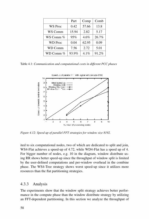
Part Comp Comb
WS Proc 0.42 57.66 13.8
WS Comm 15.94 2.82 5.17
WS Comm % 95% 4.6% 26.7%
WD Proc 0.04 62.95 0.09
WD Comm 7.56 2.72 5.01
WD Comm % 93.9% 4.1% 91.2%
Table 4.1: Communication and computational costs in different PCC phases
Figure 4.12: Speed up of parallel FFT strategies for window size 8192.
ited to six computational nodes, two of which are dedicated to split and join,WS4-Flat achieves a speed-up of 4.72, while WD4-Flat has a speed up of 4.For bigger number of nodes, e.g. 10 in the diagram, window distribute us-ing RR shows better speed-up since the throughput of window split is limitedby the user-defined computations and per-window overhead in the combinephase. The WS4-Tree strategy shows worst speed-up since it utilizes moreresources than the flat partitioning strategies.
4.3.3 Analysis
The experiments show that the window split strategy achieves better perfor-mance in the compute phase than the window distribute strategy by utilizingan FFT-dependent partitioning. In this section we analyze the throughput of
58

the parallel branches of both strategies for the fft3 SQF to complement theexperimental results.
The throughput of a node can be expressed as the ratio of the size of alogical window over the total time it takes to process it.
The total processing time T for a logical window of size N includes thefollowing components:• Time TSQF(N) for executing an SQF assuming that only one SQF is exe-
cuted on the node (the common case for the parallel branches);• Communication time Trecv(N) to receive an input logical window;• Communication time Tsend(N) to send a result stream window;• Time Tsys for performing system tasks, such as buffer management and
scheduling
T (N) = Trecv(N)+TSQF(N)+Tsend(N)+Tsys (4.1)
In the model above we assume that the SQF has a fan-out factor of one, i.e.produces one result window for each input logical window.
Let us consider the throughput of one partition of a strategy with degree ofparallelism k and logical windows of size N. The maximum throughput of oneRound Robin partition is:
T hrRR =N
T (N)(4.2)
For the same initial logical window size the window split partitioning processesk logical windows of size N
k . Hence, the maximum input throughput of oneparallel window split partition is:
T hrWS =Nk
T (Nk )
=N
kT (Nk )
(4.3)
In order for the user-defined window split partitioning to have higher through-put than the RR partitioning, the following condition must be fulfilled:
NkT (N
k )>
NT (N)
(4.4)
orT (N) > kT (
Nk
) (4.5)
Trecv(N)+TSQF(N)+Tsend(N)+Tsys > k(Trecv(Nk
)+TSQF(Nk
)+Tsend(Nk
)+Tsys)(4.6)
Under the assumption that the system overhead and the communication
59
times are approximately the same, the computational complexity of the SQFdetermines the strategy with the best throughput. Under the above assumptionthe window split is better than the window distribute if and only if:
TSQF(N) > kTSQF(Nk
) (4.7)
The fft3 SQF executes FFT with complexity O(n logn). If we ignore thelow-order terms in the complexity formula for big enough N the above re-quirement takes the form:
cN logN > kcNk
logNk
= cN(logN− logk) (4.8)
The last inequality is fulfilled for all values for the number of partitions k≥ 2.Here we need to take into account the following factors that might cause
unexpected behavior in the real experiments.• For small values of N the low-order terms might prevail and change the
inequality.• Even when the SQF complexity analysis shows an advantage for window
split, the total real advantage is smaller since communication and systemtasks costs also affect the total throughput. In situations with relativelycheap SQFs and relatively expensive communication costs, such advantagemight be negligible.
• As it can be seen from equation 4.7 whether user-defined partitioning wouldhave advantage in terms of total throughput depends on the computationalcomplexity of the SQF as well as on the existence of a particular, more effi-cient, method for parallel computation to be used. For example, we can ex-pect similar results for sort algorithms with complexity O(n logn), such asmerge-sort, but we cannot expect throughput improvement for SQFs withlinear complexity.
60

5. Definition and Management of ContinuousQueries
In this chapter we present the definition and management of continuous queries.First we describe the meta-data used for representation of continuous queriesand data flow distribution templates at the coordinator. We present the imple-mentation of the built-in library of templates constructors.
Long-running continuous queries require different management from streammanagement systems than the management of one-time queries in DBMSs.We describe the CQ management tasks performed by the coordinator dur-ing the life cycle of queries. Finally, we describe a profile-based optimizationframework for automatic generation of optimized parallel plans for expensivequery functions.
5.1 Meta-data for CQsFigure 5.1 shows the meta-data describing continuous queries at the coordi-nator. Queries are instances of type CQ. Stream objects at working nodes aredescribed at the coordinator by objects of type Mstream (a meta-stream). TheMstream properties source, dest, and interface represent the correspondingproperties of the stream objects (Sec. 3.2). In addition the stype property storesthe most specific type of a stream object, e.g., “Radio”, which is needed whena stream object is created at a working node. The functions inputs and outputsare defined on type CQ and return vectors (ordered sequences) of meta-streamobjects representing the stream on which the query is executed.
The following system procedures register input and output streams to thesystem, respectively.
register_input_stream(Charstring stype,Charstring source, Charstring interface)-> Mstream s;
register_result_stream(Charstring dest,Charstring interface) -> Mstream s;
For each input stream the user specifies its type stype, the source address ofthe program or instrument sending the stream, and stream interface to be used.
61

inputs
CQ
1 n
Dataflow
Mstream
name
source
dest
interface
outputs
n1
stypeplan
1
1
Figure 5.1: Meta-data for continuous query representation
The type of the stream must be some of the stream types defined in the system,and the interface must be valid for this stream type. The stream propertiesthat are not specified in the above procedures, are inferred by the system. Forinstance, the destination of an input stream will be set to the working nodewhere the SQFs operating on it are assigned. The name of the stream is anidentifier, generated automatically when an Mstream object is created.
The user specifies the destination address dest to which the result streamshould be sent and the stream interface to be used. Notice, that the type ofthe result stream does not need to be specified, since the system will derive itfrom the CQ specification. The above procedures create in the coordinator theobjects of type Mstream representing the streams and set their attributes.
The plan function specifies an object of type Dataflow that represents thedata flow graph for query execution. We describe the meta-data about thegraphs in the next section.
The following system procedure is a constructor for CQ objects given thedata flow graph, and the input and output streams:
cq(Dataflow d, Vector of Mstream ins,Vector of Mstream outs) -> Cq q;
An example query specification is given below:
set s1 = register_input_stream("Radio","1.2.3.4","UDP");
set s2 = register_result_stream("1.2.3.5","Visualize");
set wsplit = PCC(2,"fft3part","fft3",{},
62

Site
assigned_to
flowDataflow
widtharity
1
Node
params
fn
id
location
n
n
1
level
id
id
inputsoutputs
Figure 5.2: Metadata for specification of distributed data flow graphs
"OS-Join",{"fft3combine"});set q = cq(wsplit, {s1}, {s2});
Here the user explicitly specifies the distributed execution strategy for thequery through the PCC template, providing the system with information aboutthe degree of parallelism two and the partitioning strategy to be used, definedthrough the fft3part and fft3combine functions. To provide transparency to theuser, the system can also automatically enumerate and select an optimizedexecution plan for a given query. We will address this problem at the end ofthe Chapter.
5.2 Data Flow Graph DefinitionFigure 5.2 shows the meta-data describing data flow graphs. The graphs arerepresented by a type Dataflow with properties arity and width describingthe number of input and output streams of the graph, respectively. It is as-sumed that the input and output streams are numbered starting from zero. TheDataflow type has a number of other attributes that describe, e.g., executionstatistics of the graph, and are supported automatically by the system. Herewe skip these attributes and present only the properties important for the dataflow graph construction.
Vertices in the graph are instances of type Node with properties id that isan automatically generated unique identifier, fn that is the name of the SQFannotating the node, and params that is a vector of non-stream parameters of
63

the SQF. The function flow defined on the Node type specifies the data flowgraph in which the node participates.
Inputs and outputs are special attributes that describe producer-consumerrelationships between SQFs or a binding of SQFs to the input and outputstreams of the data flow graph. The inputs function returns a vector of ele-ments that are either other nodes or input stream numbers. The Outputs func-tion returns a vector of elements that are either other nodes or output streamnumbers. When two nodes, n1 and n2, are connected through a producer-consumer relationship, node n2 has in its inputs function value an elementequal to n1, while node n1 has n2 among the elements of its outputs function.
If a node does not consume the result of any other node in the data flowgraph, it has in its inputs function only order numbers of input streams ofthe graph. We call such a node an input point of the graph. We use the termoutput points in a graph for nodes, such that there is no other node in the graphconsuming their results. Since one node logically produces one result stream,an output point has in its outputs function only one order number of the outputstream of the graph that the node produces.
However, when a graph g1 is connected by a pipe to another graph g2, it ispossible to connect multiple nodes from g2 to consume the result stream froma single output point of g1. As a result the outputs function of the connectedoutput point will contain references to all the consuming nodes in g2. Notice,that after g1 and g2 are connected, the output points in g1 are not any moreoutput points for the composed graph.
The derived attribute level is used to store the level of a node in the topolog-ical ordering defined by the inputs function. The level of a node is computedas a sum of one and the maximum level of the nodes in the inputs functionof the node. If a node is an input point, i.e. the inputs function contains onlyinput stream numbers, the level of the node is set to zero.
The logical execution sites are instances of type Site with properties id, aunique identifier generated automatically by the system, and location, whichspecifies the name of the computing node to which the logical site is mapped.The mapping is performed by the system after the resources for the queryhave been allocated. A distributed execution is achieved by assigning graphnodes to different logical execution sites. The assignment is specified throughthe assigned_to function defined on the Node type returning an object of thetype Site.
5.3 Templates ImplementationIn this section we present the implementation of the data flow distributiontemplates from the built-in library.
64

1: function CENTRAL( f n, params,n)2: d← data f low(n,1)3: s← site()4: nd← node( f n, params,vector(0,n−1),{0},d,s)5: return d6: end function
Algorithm 1: Central template constructor
1: function PARTITION(n, tmpl, params)2: d← data f low(1,n)3: s← site()4: for i← 0,n−1 do5: APPLY_TEMPLATE(tmpl,{n,i,params},{0},{i},d,s)6: end for7: return d8: end function
Algorithm 2: Partition template constructor
5.3.1 Central ExecutionThe central template constructs a central data flow graph of one node as shownin Algorithm 1.
We use the following functions in Algorithm 1:• dataflow(arity, width) is a constructor of a dataflow object setting its proper-
ties arity (number of input streams), and width (number of output streams).The central data flow in the algorithm has n input streams as the number ofinput streams of the SQF, and one output stream.
• site() is a constructor of Site objects;• node(fn, params, inputs, outputs, flow, assigned_to) is a node constructor
setting the attributes of the node with the corresponding names.• vector(0,k) is a vector constructor that returns a vector of ordered elements
in the interval [0,k].
5.3.2 PartitioningThe partition template constructs a partitioning graph as in Figure 3.3a. Thepseudo code is given in Algorithm 2. Algorithm 2 uses the dataflow construc-tor as in algorithm 1, but here the data flow graph has arity one and width n.n nodes are created and connected to different output streams of the graph toproduce different partitions.
The template uses a system procedure apply_template (Algorithm 3) thatcreates a data flow graph by applying a template in its first parameter on a
65

1: procedure APPLY_TEMPLATE(tmpl, params, inputs,out puts,d,s)2: if template(tmpl) then . Expand compute template3: cd← apply(tmpl, params)4: BIND_INPUTS(cd,inputs)5: BIND_OUTPUTS(cd,outputs)6: for all nd ∈ nodes(cd) do7: f low(nd)← d8: if s 6= nil then9: assigned_to(nd)← s
10: end if11: end for12: else13: APPLY_TEMPLATE(“central”,{tmpl,params,count(inputs)},
inputs, outputs,d,nil)14: end if15: end procedure
Algorithm 3: Expand template or SQF invocation
vector of template parameters in the second parameter. The created nodes areincluded in a container graph d and assigned to a site s, the last parameters ofthe procedure. The inputs and outputs functions of the nodes in the graph areassigned correspondingly to the inputs and out puts parameters of the proce-dure.
The procedure contains a call to the predicate template(fn) that returns trueif the parameter fn is a name of a template constructor. The apply_templateprocedure uses two procedures to bind the nodes of the new graph to the in-puts and outputs of the container data flow graph d. Bind_inputs substitutesthose elements in the inputs functions of the nodes in a graph d that are ordernumbers of input streams (hence, the predicate numeric(k)) with the streamorder numbers specified in the inp parameter. Bind_outputs in Algorithm 5has similar functionality, but for the output points. The function nodes(d) thatreturns all nodes in a data flow graph d. It is an inverse of the flow function. Ifthe tmpl parameter is an SQF function, the procedure calls the central templateto create a graph with one node annotated with the SQF.
5.3.3 Parallel execution
The Algorithm 6 presents the pseudo code of the parallel template constructorthat creates s a parallel graph as shown in Figure 3.3b. Each of the parallelbranches is created by a call to the apply_template procedure.
66

1: procedure BIND_INPUTS(d, inp)2: for all nd ∈ nodes(d) do3: v← inputs(nd)4: for i← 0,count(v)−1 do5: if numeric(v[i]) then6: v[i]← inp[v[i]]7: end if8: end for9: inputs(nd)← v
10: end for11: end procedure
Algorithm 4: Binding inputs
1: procedure BIND_OUTPUTS(d,out p)2: for all nd ∈ nodes(d) do3: v← out puts(nd)4: for i← 0,count(v)−1 do5: if numeric(v[i]) then6: v[i]← out p[v[i]]7: end if8: end for9: out puts(nd)← v
10: end for11: end procedure
Algorithm 5: Binding outputs
5.3.4 Pipelined execution
The pipe template takes two data flow graphs and creates a new data flowgraph by copying the nodes and sites in the component data flow graphs andconnecting the copies of the input points from the second component graph tothe corresponding copies of the output points from the first component graph.Algorithm 7 shows the pseudocode. The following functions are used in thealgorithm:
• copy_nodes(d,map) creates copies of all nodes and sites in the data flowgraph d. The map parameter is a data structure that holds the mapping be-tween an original node and its copy. Algorithm 8 presents it’s pseudocode.
• get_output(d,i) is a function that returns the i-th output point of the dataflow graph d, i.e. the node for which the value of the outputs function is setto {i}.
67

1: function PARALLEL(n, tmpl, params)2: d← data f low(n,n)3: for i← 0,n−1 do . Create branch i4: APPLY_TEMPLATE(tmpl,params,{i},{i},d,nil)5: end for6: return d7: end function
Algorithm 6: Parallel template constructor
• input_points(d) is a function that returns all nodes that are input points ofthe data flow graph d.
• thecopy(nd,map) is a function that returns the copy of the node nd as spec-ified by the mapping map.
5.4 CQ ManagementContinuous queries require different management from a DSMS than the man-agement of one-time queries in DBMS. Traditionally, a one-time query in adatabase finishes when the entire result set is produced having all input dataprocessed. Since input data in stored databases are finite in size, the resultis expected to be produced in a limited time. However, in the case of con-ceptually infinite stream data a continuous query can also run infinitely, asrequired for some monitoring applications such as monitoring plant environ-ments. There are also cases when the user needs a query to run for a limitedamount of time, for instance to monitor traffic conditions only in rush-hours.Therefore, a DSMS must allow a continuous query to run for a specified timeinterval or unconditionally. It also must provide an interface for explicit termi-nation of CQs, which we call deactivation. The CQ management thus includesthe following tasks:1. Compilation of a data flow graph into an execution plan;2. Starting the execution that includes installation and activation;3. Monitoring the execution;4. Deactivation of execution.We will present each of these tasks in separate subsections.
5.4.1 CQ CompilationGiven the data flow graph and the input and result streams, the coordinatorcompiles the data flow graph into a distributed execution plan. The compila-tion algorithm contains the following main steps as shown in Algorithm 9:
68

1: function PIPE(d1,d2)2: d← data f low(arity(d1),width(d2))3: map← nil4: for all nd ∈ copy_nodes(d1,map) do5: f low(nd)← d6: end for7: for all nd ∈ copy_nodes(d2,map) do8: f low(nd)← d9: end for
. Connect copies of input points of d2 to the copies of output points of d110: for all nd2 ∈ input_points(d2) do11: v← inputs(nd2)12: for i← 0,count(v)−1 do13: nd1← get_out put(d1,v[i])14: cnd1← thecopy(nd1,map)15: cnd2← thecopy(nd2,map)16: inputs(cnd2)[i]← cnd117: out puts(cnd1)← out puts(cnd1)+ cnd218: end for19: end for20: return d21: end functionAlgorithm 7: Pipe
1. Determine node dependencies. The dependencies between nodes specifiedthrough inputs and outputs functions are analyzed and stored as a value ofthe level attribute of node.
2. Bind the nodes that are input points of the data flow graph to the inputstreams of the query. The binding uses the input stream numbers in theinputs function.
3. For each node, starting from the input points of the graph and followingan increasing order of the level function values, compile the node. Thecompilation of a node is given below.
4. Connect the SQFs that are output points of the data flow graph to the resultstreams of the CQ.
The Algorithm 9 uses the following functions and procedures:
• max_level(d) returns the maximum among the levels of the nodes in a dataflow graph d;• result_streams(n) is a multi-value function that stores the result stream ob-
jects created for the node n
69

1: function COPY_NODES(d,map)2: for all s ∈ sites(d) do3: news← copy_site(s,map)4: end for5: for all nd ∈ nodes(d) do6: newnd← copy_node(nd,map)7: assigned_to(newnd)← thecopy(assigned_to(nd),map)8: return newnd9: end for
10: end functionAlgorithm 8: Copying of a data flow
The compilation of a node presented by the pseudocode in Algorithm 10has the following steps:1. Perform a type check of the parameters of the SQF in order to derive the
type of the result stream (line 2). The stream parameters are specified ininputs function, while non-stream parameters are given in the params at-tribute of the node. The type check requires that the input streams of thenode are already bound when the node is processed. We ensure this by start-ing with the data flow input points with level value equal to 0 and followingthe SQF dependencies, i.e. increasing level values. The compiler infers thetype of the result stream from the SQF definition. The type is needed bythe result stream constructor.
2. Group the consumers of the compiled node according to their site assign-ments. For each group create a logical stream connecting the current nodeto the group of consumers. In this way the consumers in the group sharethe input stream produced by the node.
3. If both the node and the group of its consumers are assigned to the samesite, the logical stream is implemented by a stream object with a main-memory stream interface assigned to the same site (lines 8-14).If the group of consumers is assigned on a different logical site than thecurrent node, the logical stream is implemented by a pair of dual stream ob-jects using inter-GSDM stream interface (lines 15-24). One of the streams(line 16), assigned to the current node’s site, sends data from the currentnode to the site where the consumers group is assigned. The second streamobject (line 17) is assigned to the consumers’ site and receives data fromthe current node.
Algorithm 10 uses the following functions and procedures:• derive_result_type(n) checks the types of the SQF parameters and returns
the type of the result stream using the definition of the SQF annotatingthe node.
70

1: function COMPILEDFG(d)2: cq← plan_o f (d)3: LEVELS(d)
. Connect all input points to the input streams4: BIND_INPUTS(d,inputs(cq))5: success← true6: for i← 0,max_level(d) do7: for all n ∈ nodes(d) do8: if level(n) = i∧ success then9: success← compile(n)
10: end if11: end for12: end for13: if success then
. Connect the output point to the CQ result streams14: n← get_out put(d,0)15: for all outs ∈ out puts(cq) do16: result_streams(n)← result_streams(n)+outs17: end for18: end if19: return success20: end functionAlgorithm 9: Algorithm for compilation of a data flow graph (DFG)
• consumer_sites(n) is a derived function that returns all objects of type Siteto which some node is assigned that is a consumer of the argument node n;
• nextstreamid() is the system generator of stream identifiers;• mm_stream(name,stype,st) is a stream constructor using the default para-
meters for streams in main memory inside a working node. The parametersspecify the stream name, type, and a Site object representing the site wherethe stream object will be created;• inGSDM_stream(name,stype,st,src) and outGSDM_stream(name,stype,st,-
dest) are stream constructors using the default parameters for inter-GSDMstreams. The first three parameters are as described above. The last para-meter is a source address for an input stream and a destination address foran output stream object. Notice, that the dual streams have the same namebut are assigned to different sites;
• subst(v,n,s) is a procedure that substitutes the object n with the object s inthe vector v. It is used to bind a node to an input stream produced by thenode producer by the call subst(inputs(n),nprod,s2).
71

1: function COMPILE(n)2: stype← derive_result_type(n)3: if stype then4: st prod← assigned_to(n)5: for all st ∈ consumer_sites(n) do6: name← nextstreamid()7: if st = st prod then . Create stream in main memory8: s1← mm_stream(name,stype,st prod)9: result_streams(n)← result_streams(n)+ s1
10: for all n1 ∈ out puts(n) do11: if st = assigned_to(n1) then12: SUBST(inputs(n1),n,s1)13: end if14: end for15: else . Create inter-GSDM stream of two dual stream objects16: s1← outGSDM_stream(name,stype,st prod,name(st))17: s2← inGSDM_stream(name,stype,st,name(st prod))18: result_streams(n)← result_streams(n)+ s119: for all n1 ∈ out puts(n) do20: if st = assigned_to(n1) then21: SUBST(inputs(n1),n,s2)22: end if23: end for24: end if25: end for26: return true27: else28: return f alse29: end if30: end functionAlgorithm 10: Node Compilation
72

• result_streams(n) is a multi-value function that stores the result streams ofa node n. It is used later on by the installation. The function contains astream object for each group of consumers on different site.
5.4.2 MappingThe compilation of a data flow graph creates an execution plan where dis-tribution is specified in terms of logical execution sites. In order to start theexecution, logical sites have to be mapped to physical computing nodes allo-cated by the resource manager of the coordinator. Here we assume that thecomputing resources have been allocated, so that the coordinator has on itsdisposal list of available computing nodes to be used for the query execution.
The mapping between logical sites and nodes is created by a system proce-dure that sets the location attribute of all Site objects in the data flow graph.Currently we always do one-to-one mapping between a logical site and a com-puting node to maximize the parallelism. Other mappings will be investigatedas a future work.
1: procedure START(d)2: for all g ∈ sites(d) do . All logical sites in d3: START_WN(location(g), id(g))4: end for5: end procedure
Algorithm 11: Starting Working Nodes
When the mapping is set, the resource manager starts GSDM working nodeson the allocated computing nodes (Algorithm 11). When a working nodestarts it first registers itself to the name server and to the coordinator, and thenstarts its server loop in which it listens for the commands from the coordinatorand data messages.
5.4.3 InstallationThe installation of a continuous query consists of creating data structures andobjects representing an executable plan at the working nodes. Algorithm 12shows the main steps in the installation. There is no specific order of instal-lation between working nodes, but internally at each node it follows nodedependencies downstream (for loop in line 5).
The installation procedure is overloaded for the case when a stop condi-tion is associated with the query. In this case, the condition is installed onlyat the input points of the data flow graph since the deactivation propagatesdownstream.
73

1: procedure INSTALL(d)2: for all g ∈ wn(d) do3: maxlev← maxlevel(d,g)4: minlev← minlevel(d,g)5: for l← minlev,maxlev do6: for all v ∈ nodes(d) do7: if level(v) = l∧assigned_to(v) = g then8: for all s ∈ inputs(v) do9: INSTALL_STREAM(s)
10: end for11: INSTALL_SQF(v)12: for all s ∈ result_streams(v) do13: INSTALL_STREAM(s)14: end for15: end if16: end for17: end for18: end for19: end procedure20: procedure INSTALL(d,kind,value)21: INSTALL(d)22: for all v ∈ input_points(d) do23: INSTALL_STOP(v,kind,value)24: end for25: end procedure
Algorithm 12: CQ Installation
5.4.4 ActivationDuring the activation the SQFs in the execution plan are initialized and addedto the list of active operators scanned by the scheduler. Algorithm 13 showsthe activation steps. Since a node result stream is pushed to the consumers,the system must ensure that the consumers are already listening when a nodestarts producing data. This is achieved by activating the nodes in an order thatis inverse to the node dependencies, i.e. upstream.
5.4.5 DeactivationDeactivation of a continuous query consists of synchronized stopping of allSQFs in the query plan. The deactivation can be triggered by a stop conditionassociated with the query or performed on explicit command from the user.
Since the data flow graph runs in a distributed environment, we have devel-
74

1: function ACTIVATE(d)2: success← true3: for i← max_level(d),0 do4: for all v ∈ nodes(d) do5: if level(v) = i∧ success then6: success← activate(v)7: end if8: end for9: end for
10: return success11: end functionAlgorithm 13: CQ Activation
oped a mechanism for synchronizing the deactivation on different nodes. It isinitiated on all the input points of the data flow graph. Once they are deacti-vated, they propagate the deactivation to the consumers downstream, whichon their turn are deactivated and propagate the deactivation until it reaches theoutput points of the execution plan.
5.5 Monitoring Continuous Query Execution
One of the important characteristics of continuous queries is that they arelong-running by definition. Hence, it is highly probable that the system willexperience changes in the execution environment during the runtime of a CQdue to changing rates of the source streams, changing availability of resources,or registering of new CQs that share resources with the existing ones.
Therefore, to provide efficient processing of CQs, the system should moni-tor the execution and adapt, if possible, the execution plans to fit better to thechanged conditions. GSDM has a monitoring subsystem consisting of statis-tics collector modules in the working nodes and the coordinator. The query ex-ecutor and the scheduler of working nodes invoke various statistics primitivesto update the statistical meta-data. The most important parameters for moni-toring in a distributed stream processing system are stream rates, CPU timesfor SQF executions, memory availability, memory utilization by the streambuffers, and communication costs. The statistics collector module of the co-ordinator periodically gathers statistical information from working nodes andperforms analysis of the overall CQ performance.
75

5.6 Data Flow OptimizationThe purpose of data flow optimization is to create an optimized data flowgraph for a given continuous query. The optimization provides higher degreeof transparency than the specification of queries through templates where thedegree of parallelism and the partitioning strategy are specified explicitly. Theoptimizer automatically generates distributed execution plans and selects anoptimized plan using some optimality metric. Traditionally database queryoptimizer functionality consists of plan enumeration, generating plans in thespace of possible plans, and a cost estimation model on which the selection ofan optimized plan is based.
We have developed a CQ optimizer for PCC with limited functionalitythat optimizes parallel execution plans for a single expensive SQF. Next, weshortly describe the components of the current CQ optimizer. The optimiza-tion of the individual SQFs relies on traditional query optimization.
5.6.1 Estimating Plan CostsTraditional cost models rely on relatively accurate estimates of the costs ofindividual operators that are used to estimate the cost of the entire plan. How-ever, in an extensible system such as GSDM executing user-defined functionsover user-defined data, the cost model of individual functions might be hard todefine or obtain from the author of the code. Furthermore, to allow utilizationof processing resources allocated on-demand among computers with differ-ent performance parameters, the system would need to support a separate costmodel for each architecture.
Therefore, the CQ optimizer selects an optimized plan based on trial runsthat collect execution statistics rather than based on a cost estimate model. Theoptimizer collects statistics about the utilization time of working nodes, whichis a sum of the SQF’s processing times, the communication time, and thetime spent in system tasks. The working node with maximum utilization timelimits the throughput achievable by the data flow graph and hence we definean optimality metric (cost) of a plan as the maximum utilization time amongthe utilization times of working nodes is the plan. We select an optimized planby selecting the plan with the lowest utilization time. In order to compare thestatistics of several plans, the trial runs use the same cluster and work on astream segment with equal size.
5.6.2 Plan EnumerationA naive plan enumeration for PCC has been implemented as follows:1. The maximum degree of parallelism is specified as a system parameter.
76

Plan Enumeration
Compilation
Run
CQ Specification
Deactivation
Data Flow Graph
Execution Plan
Running CQ
Trial Run
Plan Selection
Optimized
Execution Plan
Statistics
CQ Optimizer
Figure 5.3: Life cycle of an optimized CQ
2. Plans for partitioned parallelism are generated using the PCC template con-structor.
3. A function registry contains meta-data about the valid parallel strategiesand their parameters for a given SQF. Both the valid stream partitioningstrategies and the valid degrees of parallelism are specified in the registry.
4. The enumerator generates different plans by using the PCC template andvarying the strategy (i.e. window split or window distribute) and the validdegrees of parallelism. The enumeration of plans for a given strategy stopswhen a plan has been generated such that either the maximum degree ofparallelism or the resource limit is reached.Each of the graphs is compiled, run in a trial mode, and statistics about the
execution is stored in the coordinator’s metadata by the statistics collector.The CQ optimizer then chooses an optimized data flow graph using the sta-tistics collected and the above model for optimality. The life cycle of the CQoptimized in this way is shown in Figure 5.3.
The optimizer is implemented as a function with the following signature:
opt(Charstring templ, Charstring fun,Vector params, Vector inpstr) -> Dataflow d;
77

It takes as parameters the function fun to be executed, its parameters, and inputstreams inpstr. The first parameter is a template to be used for plan enumer-ation and currently only PCC is supported. The optimizer assigns automati-cally an output stream to collect statistics from trial runs. The result of the optfunction is an optimized data flow graph for the provided parameter functionfun. Using the CQ optimizer functionality, the continuous query on page 63 isspecified by an alternative template constructor as follows:
set q = cq(opt("PCC","fft3",{},{s1}), {s1}, {s2});
The optimized plan is set by the cq constructor to the plan property of thequery and used when the run(q) procedure starts the execution.
In the example above, plans with RR and user-defined stream partitioningare generated with different degrees of parallelism and the plan with best exe-cution time from the trial runs is selected. In this way transparency is providedto the user, so that only the SQF fft3 needs to be specified in the query, ratherthan all explicit parameters of the PCC template as in the example on page 63.
The current CQ optimizer provides automatic optimization of paralleleliz-able expensive SQFs using the PCC pattern. The experiments show that theoptimization framework with trial runs and statistics collection is feasible, butit needs to be generalized in several important directions:• Sophisticated plan enumeration. Since the naive enumeration of plans might
create very big space of possible data flow graphs, in order to make the op-timization efficient it is important to develop heuristics about which plansto generate and what order to follow during the generation. For example,enumeration strategies such as random walk of search space, binary search,or greedy can be investigated. The importance of such heuristics is evenbigger in our setting than for cost-based optimization, because rather thancomputing the cost, the CQ optimizer runs a plan in a trial mode.
• Optimality model. Alternatively to the maximum throughput metric, othermetrics such as latency and precision can be used. Furthermore, multi-criteria optimality model combining several metrics might show to fit bettersome applications.
• The optimization framework needs to be generalized to use different distri-bution templates besides the PCC template. For example, if a user specifiesa pipeline of two SQFs, the CQ optimizer has to enumerate plans whereeach stage of the pipe is parallelized independently of the other by, possi-bly, different degrees of parallelism and partitioning strategies, and planswhere the stages in the pipeline are executed together by defining a meta-SQF that encapsulates them, which on its turn is parallelized by some datapartitioning.
78

6. Execution of Continuous Queries
This chapter presents the execution of continuous queries at working nodes.First, we describe the implementation of operators executing SQFs and inter-GSDM communication. Next, we present the scheduling policies used by thescheduler. Finally, we describe important observations concerning the systemperformance.
6.1 SQF ExecutionThe main execution primitive is an execute operator that sets up the envi-ronment and applies an SQF over its input streams and other parameters toproduce logical windows in the SQF’s result stream. Thus, the execution planis composed of instances of the execute operator, each executing a particu-lar SQF.
6.1.1 Operator StructureFor each SQF assigned to a working node the installation procedure createsan internal data structure (an operator) that contains the characteristics of theSQF as needed for execution by the execute operator. The structure is shownin Figure 6.1. The id slot stores the unique identifier of the SQF. The identi-fiers are generated automatically by the coordinator when the nodes in the dataflow graph are created. The SQF slot is a pointer to an object of type Functionrepresenting the SQF to be executed. A paramlist stores a list of all parametersof the SQF. An inputstreamlist contains a list of stream objects that are para-meters of the SQF, where for each stream there is an internal local buffer ofpointers to the current logical windows in the stream. As we described in sec-tion 3.2.1 this buffer is accessed by the window functions in the SQF definitionproviding for SQF referential transparency.
The outputstreamlist holds a list of result streams of the SQF as determinedduring the compilation. Typically, the list contains one result stream object,but it is also possible to have more than one if the SQF has several consumersand they are assigned to different execution sites. In the latter case a differ-ent result stream object is created for each execution site where some SQF-
79

repetitionstop
condition
output
stream
list
stat
input
stream
list
paramlistSQFid
timecountlast
exec
first
exec
Operator
Statistics
state
Figure 6.1: Operator structure
consumer is assigned (Algorithm 10). The logical windows from the SQFexecution are inserted into each of the streams in the outputstreamlist.
The execution of long-running CQs is usually monitored by collecting andanalyzing execution statistics. For each SQF there is a statistics data structurestoring the initial and last time of execution, the number of executions, andthe total processing time. The stat slot in the operator structure is a pointer tothe corresponding statistics structure.
The stopcondition slot stores the stop condition associated with the SQF.Three kinds of stop conditions are supported in the current implementation:time-based, count-based1 and unconditional. The time-based and count-basedstop conditions are installed during the CQ installation by setting the stopcon-dition slot.
The repetition slot is used to set up an upper bound for the number of exe-cutions scheduled in one scheduling period. It is determined by the schedul-ing policy (to be explained below). The real number of executions might besmaller since it also depends on the data available.
Some SQFs, such as S-Merge, need to keep state in between subsequentexecutions. The state slot in the operator structure allows to store such state.To provide state initialization and clean-up, a pair of operations initializationand cleaning-up can be associated with the SQF. The operations are calledduring the activation and deactivation of the SQF, respectively.
An SQF can be in one of the following three states, illustrated in Figure 6.2:uninstalled, installed, and active, where a state transition is performed on acommand from the coordinator or from the scheduler. As described in Chapter2, all operator structures for SQFs installed at a working node are stored in ahash table installed operators with key the SQF’s id. The active operators
1We used a count-based stop condition to provide an equal stream segment size for all experi-ments.
80
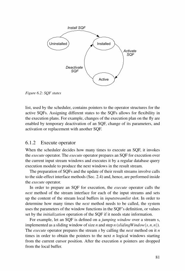
Uninstalled Installed
Active
Install SQF
ActivateSQF
DeactivateSQF
Figure 6.2: SQF states
list, used by the scheduler, contains pointers to the operator structures for theactive SQFs. Assigning different states to the SQFs allows for flexibility inthe execution plans. For example, changes of the execution plan on the fly areenabled by temporary deactivation of an SQF, change of its parameters, andactivation or replacement with another SQF.
6.1.2 Execute operatorWhen the scheduler decides how many times to execute an SQF, it invokesthe execute operator. The execute operator prepares an SQF for execution overthe current input stream windows and executes it by a regular database queryexecution module to produce the next windows in the result stream.
The preparation of SQFs and the update of their result streams involve callsto the side-effect interface methods (Sec. 2.4) and, hence, are performed insidethe execute operator.
In order to prepare an SQF for execution, the execute operator calls thenext method of the stream interface for each of the input streams and setsup the content of the stream local buffers in inputstreamlist slot. In order todetermine how many times the next method needs to be called, the systemuses the parameters of the window functions in the SQF’s definition, or valuesset by the initialization operation of the SQF if it needs state information.
For example, let an SQF is defined on a jumping window over a stream s,implemented as a sliding window of size n and step n (slidingWindow(s,n,n)).The execute operator prepares the stream s by calling the next method on it ntimes in order to obtain the pointers to the next n logical windows startingfrom the current cursor position. After the execution n pointers are droppedfrom the local buffer.
81

If an SQF is defined using a sliding window, i.e. slidingWindow(s,n,1), itwill be similarly prepared for the first execution by n calls to the next methodon the stream s, but only one pointer will be dropped after the execution. Allthe following executions will be prepared by one call to the next method, sincethe rest n−1 pointers are remaining in the buffer after the previous execution.In both cases the sliding window function will return a vector of n logicalwindows relative to the current cursor position.
SQFs with time-based sliding window functions are prepared based on thetime stamp characteristics of data. If an SQF is defined using a time-basedsliding window, i.e. timeWindow(s,span), the execute operator calls the nextmethod to retrieve the pointer to the next available logical window with timestamp ts and drops from the local buffer all pointers to data with a time stampsmaller than ts− span.
After the data from the input stream is prepared in the local buffers, the exe-cute operator executes the SQF by the regular database query engine in AmosII, providing function parameters from the paramlist slot of the operator struc-ture. The produced result logical windows are added to the registered resultstreams of the SQF by calls to the corresponding insert interface methods.
If an SQF is scheduled when there is not enough stream data, the windowfunctions return nil and the call to the SQF does not create result windows.
6.1.3 Implementation of S-Merge SQFThe semantics of S-Merge SQF is to merge data from many streams preserv-ing the order determined by an ordering attribute, in our case a time stamp.Assuming that the order is preserved inside each of the merged streams, theexecution is just a selection of the logical window with the smallest time stampamong the current logical windows of all the merged streams.
S-Merge is designed to merge arbitrary number of streams and hence itsfirst parameter is of type Vector of Stream.
The semantics of S-Merge requires all the merged streams to have data inorder to compute the smallest time stamp. However, delays due to distrib-uted processing and communication, loss of data, or end-of-stream conditionmay create a situation when some of the stream buffers are empty. In orderto provide non-blocking behavior in such a situation, the operator is associ-ated with a time-out parameter. If data on a stream is not available, S-Mergewaits for time-out time period after the first attempt to obtain it. If data is stillnot available after this period, S-Merge assumes that data has been lost andselects the logical window with the smallest time stamp among the streamswith non-empty buffers. If a delayed logical window comes later on, S-Mergeignores it to preserve the order of already produced result stream. The S-Mergepseudocode is shown in Algorithm 14.
82

1: function S-MERGE(vs, timeout)2: res← nil3: empty← check_empty_bu f f ers(vs)4: if (empty∧ timer = nil) then5: timer← now() . Start timer if empty buffer is detected6: else if (¬empty)∨ (empty∧ timeout_exp(timer, timeout)) then7: ts← min_ts(vs)8: s← stream_min_ts(vs, ts)9: MARK(s)
10: timer← nil11: if ts≥ last_ts then12: res← currentwindow(s)13: last_ts← ts14: end if15: end if16: return res17: end functionAlgorithm 14: S-Merge Algorithm
The algorithm uses the following functions and procedures:• check_empty_buffers(vs) is a predicate that checks that all the buffers of
streams in the vector vs contain data.• timeout_exp(timer, timeout) is a predicate that checks for time-out expira-
tion.• min_ts(vs) finds the minimum time stamp among the time stamps of the
current logical windows in the streams vs;• mark(s) puts a marker to the stream from which the logical window with
minimum time stamp is chosen. The execute operator uses the mark todelete the pointer in the local buffer for this stream when S-Merge finishes;
The selected logical window with minimum time stamp is emitted only ifits time stamp does not violate the result ordering (lines 11-14). Values oftimer and last_ts are kept in the S-Merge state in the state slot of the operatorstructure.
6.1.4 Implementation of OS-Join SQF
The semantics of the OS-Join SQF is to join data from multiple streams ontheir ordering attribute time stamp and to apply a combining function on thejoint data preserving the order in the result stream. The first parameter is oftype Vector of Stream, and the second is the combining function to be applied.
83
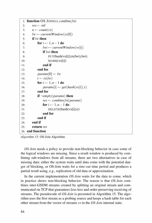
1: function OS-JOIN(vs,combine f n)2: res← nil3: n← count(vs)4: lw← currentWindow(vs[0])5: if lw then6: for i← 1,n−1 do7: lwi← currentWindow(vs[i])8: if lwi then9: PUT(hash(vs[i]),ts(lwi),lwi)
10: MARK(vs[i])11: end if12: end for13: params[0]← lw14: t← ts(lw)15: for i← 1,n−1 do16: params[i]← get(hash(vs[i]), t)17: end for18: if ¬empty(params) then19: res← combine f n(params)20: for i← 1,n−1 do21: DELETE(hash(vs[i]),t)22: end for23: end if24: end if25: return res26: end functionAlgorithm 15: OS-Join Algorithm
OS-Join needs a policy to provide non-blocking behavior in case some ofthe logical windows are missing. Since a result window is produced by com-bining sub-windows from all streams, there are two alternatives in case ofmissing data: either the system waits until data come with the potential dan-ger of blocking, or OS-Join waits for a time-out time period and produces apartial result using, e.g., replication of old data or approximation.
In the current implementation OS-Join waits for the data to come, whichin practice shows non-blocking behavior. The reason is that OS-Join com-bines inter-GSDM streams created by splitting an original stream and com-municated on TCP that guarantees loss-less and order-preserving receiving ofstreams. The pseudocode of OS-Join is presented in Algorithm 15. The algo-rithm uses the first stream as a probing source and keeps a hash table for eachother stream from the vector of streams vs in the OS-Join internal state.
84

The following functions and procedures are used in Algorithm 15:• hash(s) is a function that given a stream object returns the hash table for
the object in the internal state of OS-Join.• put(h,k,val) inserts the value val in the hash table h using the key k• get(h,k) retrieves the element with key k.• delete(h,k) deletes the element with key k.• empty(v) is a predicate that checks if the vector v has elements with nil
values.In order to implement the time-out alternative that is non-blocking in gen-
eral without the above assumptions holding in our case the time-out parametershould be added as in S-Merge. In addition there is a need for specification ofpartial results computations, e.g., by an additional parameter partcombine, thatis a function called to compute the partial results.
6.2 Inter-GSDM communicationThe communication between GSDM servers is message-based where the mes-sages contain commands to be executed at the receiving server. GSDM serverscan send messages synchronously or asynchronously. When a message is sentsynchronously, the server executes the command contained in it and sends theresult of the execution back to the server sending the request. The requestingserver waits for the result before continuing its work.
When an asynchronous message is sent to a server, the sending server con-tinues its work without waiting for the result. The message is annotated withinformation whether the result of the execution should be stored at the re-ceiver to be retrieved later on. The command in the message is executed at thereceiving server and the result is stored locally if specified so.
The coordinator commands to the working nodes are implemented as syn-chronous messages. The predefined primitives include, e.g. the installationand activation commands:
install_stream(Charstring stype, Charstring sname,Charstring srcaddr, Charstring destaddr,Charstring interf)-> Stream
install_SQF(Charstring id, Charstring SQFname,Vector strargs, Vector args)-> Boolean
install_stop(Charstring id, Charstring cond,Number val) -> Boolean
activate(Charstring id)-> Boolean
Furthermore, arbitrary commands can be sent to the working nodes, e.g. forsetting some system parameters such as the size of the database image in main
85

memory. By sending coordinator commands as synchronous messages statusinformation is atomically provided to the coordinator.
Stream data are pushed between working nodes using asynchronous mes-sages without waiting for the result of message execution. They contain acall to the insert method of the stream interface for the corresponding remoteinter-GSDM stream object and the data to be inserted.
6.3 SchedulingThe work of the CQ engine is controlled by its scheduler. It executes a loopwhere in each iteration the active SQFs are executed on the current streamdata. Through this loop the CQ engine achieves continuous execution of CQs.
The scheduling policy affects substantially the system performance. It isdetermined by two components: how periods of work (loop iterations) are or-ganized and how SQFs are scheduled inside a period. We call one iteration ofthe scheduler loop scheduling period. In each scheduling period the schedulerallocates resources for three groups of tasks:• Communication: the system checks for incoming inter-GSDM messages
with commands or data.• SQFs: the active operators list is scanned and each SQF there is checked
and eventually scheduled and started.• System tasks: for example management of stream buffers is performed pe-
riodically and SQFs are checked for deactivation.
6.3.1 Scheduling periodsTwo scheduling policies with respect to the length of the scheduling periodwere implemented, evaluated, and shown to fit in different situations.
The first scheduling policy has fixed length of the scheduling periods, wherethe length is called turn-around time. Its purpose is to control the maximumrate at which data is consumed from the external input streams and to preventin this way overload situations at down-stream working nodes. It also providesregular inter-arrival intervals for the stream data at the consuming servers.
The policy is implemented by a special sleep task that causes idling of theprocessor to the end of the scheduling period. If the execution time for allthe tasks in a period is bigger than the period turn-around time, the sleepis skipped and the scheduler sends a message to the coordinator notifying itabout overload.
The second scheduling policy does not have fixed length scheduling periodand hence we call it variable-length. The length of a given scheduling perioddepends on the active SQFs and the amount of unprocessed stream data. When
86

the engine finishes with the processing tasks in the current period, it startsa new period, checks for new data, and schedules their processing. In otherwords, the new period starts immediately after the work in the current periodfinished, so that data that has come in the meantime does not need to waitunnecessarily. By contrast, with fixed-length period new data has to wait untilthe beginning of the next period even if the current processing has finishedand the system is idling.
6.3.2 SQF SchedulingIn the time frame of one scheduling period different policies are possible withrespect to the execution order among the SQFs and the number of executionsfor each SQF. We call this SQF scheduling policy.
Currently, the execution order among several SQFs is determined by theirorder in the active operators list. Scheduling problems concerning orderingof stream operators are active area of research of stream processing engines[9, 18]. Most projects work in the context of a large number of relatively cheapoperators installed at the same server, which makes the ordering of operatorsan important part of the scheduling. By contrast, we do not address SQF or-dering problem and use a simple queue-based ordering since our focus areexpensive SQFs split into multiple instances for parallel processing. In thissettings, most of the servers execute a single expensive SQF over a data parti-tion.
We implemented the following two SQF scheduling policies concerning thenumber of scheduled executions:1. Fixed-number SQF policy determines the number of SQF executions per
scheduling period as specified in the repetition slot of the SQF.2. Greedy SQF policy checks the amount of unprocessed data in the input
stream buffers and based on that determines the number of SQF executionsfor the current period.The scheduling policy with fixed number of repetitions is applicable for all
SQFs, but is especially useful for the SQFs that are input points of the dataflow graphs. Fixing the number of executions per scheduling period togetherwith fixing the length of the period by the turn-around parameter allows thesystem to control the execution rates of the SQFs that are input points of thedata flow graph and, hence to control the rate with which the system “con-sumes” external stream data.
The greedy scheduling intuitively allows the system to do as much work asit can and as soon as possible. It requires that the scheduler is able to checkthe amount of unprocessed data and their time stamps. We combine greedySQF scheduling with variable length periods on internal working nodes toprocess as much data as possible and as soon as the data has been received,
87

given that there are available processing resources. We do not use greedy SQFscheduling in combination with fixed-length period, since in overload situa-tions greedy scheduling might schedule a big number of executions that ex-ceeds the turn-around time of a fixed-length period.
The scheduling period and the SQF scheduling policy are determined bythe coordinator using the above rule about the input points of the data flowgraph and their assignments to working nodes.
For each SQF in the active list, the scheduler performs the following steps:1. Checks the stop condition of the SQF. If it is true, the SQF is not scheduled.2. Checks if the SQF has fixed number of repetitions per scheduling period.
If so, the number of scheduled executions is set to the value of the repeti-tion slot.
3. If the SQF does not have fixed number of repetitions, the scheduler usesgreedy policy, i.e. determines the number of scheduled executions basedon the amount of unprocessed data and the SQF parameters.
6.3.3 Scheduling of System Tasks
At the end of each scheduling period system tasks might be scheduled as fol-lows:• The buffer manager is called periodically to clean the stream buffers from
data that all the SQFs have processed. A system parameter determines howoften the buffer manager should be invoked.
• The scheduler checks the stop conditions of the SQFs and invokes the de-activation procedure if needed.
6.3.4 Effects of scheduling on system performance
We conducted several experiments to investigate the effect of different schedul-ing policies on the overall system performance. We measured the performanceby the average response time (latency) that a logical window spends in the sys-tem, the load of the nodes, and the time spent in communication.
The purpose of the first experiment is to illustrate the effect of fixed-lengthand variable-length scheduler periods on the latency. We set up a data flowgraph of two working nodes, WN1 and WN2, where WN1 sends logical win-dows regularly to WN2, which executes a very fast identity SQF. The firstnode uses fixed-length scheduling to provide regular inter-arrival intervals atthe second node. Since an identity SQF is very cheap, the load of both workingnodes is determined by the communication costs and is very low. The mainsource of latency in this case is the time for communication and the waitingtime due to the scheduling policy.
88

Turn-around Rate in LW Load % Lat Fixed Lat Var
0.08 12.5 3.94 0.009 0.0044
0.1 10 3.18 0.104 0.0044
0.2 5 1.74 0.198 0.0044
0.3 3.33 1.18 0.302 0.0046
Table 6.1: Latency with fixed and variable length scheduling period
Table 6.1 shows the measured load and latency for logical windows of size2048 and different input stream rates. When WN2 uses fixed-length schedul-ing, we measure latency that increases proportionally to the length of thescheduling period. The reason is that when a logical window comes to theworking node after the scheduling period has started, it waits for the nextscheduling period in order to be processed. The actual waiting time dependson the synchronization between the data arrivals and the beginning of thescheduling periods.
When WN2 uses variable-length scheduling period, the system checks theTCP sockets for incoming data messages and processes them as soon as theprevious period finishes. Since the node has low load this means immediateprocessing of the incoming logical windows. We measured a constant latencyof about 0.0044 sec. (last column in the table) for different input stream rates,which can be attributed to the communication latency.
This experiment shows that the variable-length scheduling gives stable andshorter latency than the fixed-length scheduling when working nodes havelow load.
The purpose of the second experiment is to investigate whether the advan-tage of variable-length period still holds when the system load increases. Wechoose again a logical window size of 2048 (approximately 50 KB) and a dataflow graph of two working nodes, where the second one executes the fft3 SQFwith processing cost of 0.107 sec. per logical window. We increased gradu-ally the system load by increasing the input stream rate. The measurements forthe load and latency are shown in table 6.2. We measured the variable-lengthscheduling with two versions: one with greedy SQF scheduling, and one witha number of repetitions fixed to one. The measurements of both versions arevery similar2 and presented together in the last column in table 6.2.
Again the variable length period scheduling shows smaller and stable values
2In the case of under load the inter-arrival time is longer than the processing time for a logicalwindow. Hence, assuming regular inter-arrival intervals, the greedy SQF scheduling de factoschedules the SQFs for either zero or one execution, which gives the same effect as the schedul-ing with fixed-number repetitions equal to one.
89

Turn-around Rate(LW) Load % Lat Fixed Lat Var
0.3 3.3 36 0.115 0.110
0.2 5 57 0.31 0.111
0.15 6.6 73 0.259 0.111
0.12 8.33 94 0.169 0.112
Table 6.2: Latency with fixed and variable length scheduling period
Turn-around Rate(LW) Lat Comm WN1
0.1 10 0.553 0.266
0.09 11.1 1.149 0.266
Table 6.3: Latency at the receiver and communication overhead at the sender withfixed-number SQF scheduling
of the latency: we measure an average latency 0.111 out of which 0.107 is thefft3 processing cost. From this experiment we can conclude that the variablelength scheduling period indeed processes logical windows as soon as theycome, given load up to the measured 94%. Latency with fixed length periodis bigger and not proportional to the turn-around length, but varies dependingon how long logical windows need to wait until new period starts.
The goal of the third experiment is to investigate the trade-offs betweenfixed-number and greedy SQF scheduling when the system is overloaded. Weincreased the stream rate to values for which the average inter-arrival time isshorter than the processing time for a window. Tables 6.3 and 6.4 show theresults for inter-arrival interval set to 0.1 and 0.09, respectively, given the fft3processing cost of 0.107. We observe that the greedy scheduling shows shorterlatency than the fixed-number scheduling, but the communication times forsending windows increase rapidly at the sender node WN1. The reason is thatsince the processing cost is bigger than the inter-arrival time, during someperiods more than one window come and are scheduled by greedy. This in-creases the length of the period and postpones the moment when next data isread from the TCP sockets. In other words, the GSDM server does not con-sume data from the TCP buffers in a timely manner, which results in fillingthe buffers and activating the TCP flow control mechanism. As a result thecommunication cost for sending logical windows at the first GSDM node in-creases and the actual rate of sending decreases, e.g. to 9.47 instead of 10 asit is set.
This experiment shows that in the case of overloading, greedy scheduling
90

Turn-around Rate(LW) Lat Comm WN1
0.1 9.47 0.393 2.77
0.09 9.58 0.43 3.66
Table 6.4: Latency at the receiver and communication overhead at the sender withgreedy SQF scheduling
would activate the TCP flow control mechanism and through it would eventu-ally reduce the rate at the sender due to increased communication overhead.Therefore, an important system parameter to monitor for system overload isthe communication time at sending nodes. When this time increases abovesome threshold the GSDM engine should take actions to reduce the inputstream rate in a controllable way. Notice, that the overload at the downstreamworking node does not cause local loss of data since TCP is used for inter-GSDM communication. Instead, the input rate at the upstream working nodereduces, i.e. new incoming data is accumulated and eventually dropped on theentry of GSDM before any processing cost to be spent on it.
If overload occurs with fixed SQF scheduling policy at the receiving node,there will be periods when the number of windows scheduled for process-ing is less than the number of windows received and not processed. Hence,data accumulates in the stream buffers and their latency increases as shown inTable 6.3.
Therefore the overload in this case is detected by monitoring the state of thestream buffers for overflow. The system needs a policy to apply when streambuffers are filled up, but such a policy has not been implemented yet. Themost common overload policy in this case is load shedding [83] which dropssome of the data without processing based on some rules. Notice, that dataloss due to the shedding would occur at the receiver node after the streamwindows have been processed by at least the GSDM-sending node. In thecurrent application the source streams are received using the UDP protocoland data loss occurs at the input working nodes in case of overload.
Having investigated the effects of the scheduling on the communication andprocessing, we choose to use greedy SQF scheduling with variable-length pe-riods for the internal working nodes, including the parallel working nodes.Under internal working nodes we mean those that do not have SQFs operatingon external streams. In case of overload, greedy scheduling causes communi-cation overhead at the sender - the partitioning node, which allows the systemto start dropping data before it is processes by the remaining, more costly, partof the data flow in a way that does not affect the parallel branches.
In the same situation fixed-number scheduling at parallel nodes would start
91

dropping data. However, this dropping would not be synchronized among theparallel branches, thus causing higher percentage of dropped result windowsfor window split strategy due to dropped sub-windows. Furthermore, part ofthis dropping would actually happen at the combining node after the expensivework (computational SQFs) has been done.
6.4 Activation and DeactivationThe activation of an SQF includes two steps: adding the operator structurefor the SQF to the list of active operators, and calling an init operation. Thelatter opens the SQF’s input and result streams by calls to the open method oftheir stream interfaces. For SQFs with foreign implementation, the associatedinitialization operation is also performed that prepares the SQF internal state.
The deactivation starts at the input points of the data flow graph and prop-agates downstream. The propagation of the deactivation in a distributed envi-ronment is currently performed by sending a special end-of-stream messageto the stream consumers notifying that there will not be any more data on thisstream. Therefore, each SQF has an implicit stop condition that evaluates ontrue if all the input streams of the SQF have empty buffers and have receivedthe end-of-stream control message.
At the end of each scheduling period the scheduler checks the SQF’s ex-plicit and implicit stop conditions and issues a command for deactivation ofthe SQF if some of them evaluates on true. The deactivation includes threesteps: removing the SQF from the list of active operators, sending the end-of-stream control message to the consumers of its result stream, and calling aclean-up operation.
The clean-up operation closes the input and result streams by calls to theclose method of their stream interfaces, and performs the associated with theSQF cleaning-up operation. The close method for a shared stream does notdestroy the stream buffer, but only nullify the cursor in the stream buffer forthis particular SQF.
After deactivation the operator structure remains in the hash table of theinstalled operators and the SQF can be activated again later on.
6.5 Impact of MarshalingIn a distributed stream processing system data communication is intensive.The experiments with the GSDM prototype show the importance of a carefullydesigned stream communication in order to achieve good system performance.
We experimented two encodings for the scientific data. In the initial im-plementation the encoding was character based so that all numbers had to be
92

0
10
20
30
40
50
60
70
80
Partition FFT Combine
WD-Flat
WD-Tree
WS-Flat
WS-Tree
Figure 6.3: Real time spent in partition, FFT, and combine phases of the parallel-4strategies for logical window of size 8192, fast implementation, and character mar-shaling.
parsed. We measured the cost for marshaling and de-marshaling of logicalwindows containing vectors of complex numbers into character format whensent to and received from the TCP sockets. This cost was so high in compar-ison with the computational costs, that the parallel execution strategies got abottleneck in the partition and combine nodes already with degree of paral-lelism four. Figure 6.3 from [45] shows the saturation of the communicatingpartition and combine nodes for the fast FFT implementation, logical windowof size 8192, with character marshaling, to be compared with Figure 4.11b forthe same size and implementation, but with binary marshaling.
To address this problem, we replaced the encoding of logical windows intoa binary format. As a result the size of the communicated data decreases withapproximately 50% and the time spent on (de)marshaling was substantially re-duced by 6 to 10 times. This is illustrated in Figure 6.4 showing the times formarshaling and de-marshaling of logical windows with binary and characterencoding. The times increase linearly with the logical window size for mar-shaling into and from character format. We observe linear increase for mar-shaling into binary format for sizes bigger than 1024, while for small windowsizes the overhead for calling the marshaling function for a window becomessubstantial in comparison to the marshaling operation itself. The improvementachieved by using binary format is between 6 for small sizes to 10 times forbig logical windows. The times measured for the binary representation in-cluded copying of a logical window from the internal GSDM format into bi-nary format. Therefore, those times can be further improved by changing theimplementation to avoid the copying. However, the current implementation isefficient enough to allow for data flow graphs with high degree of parallelism
93
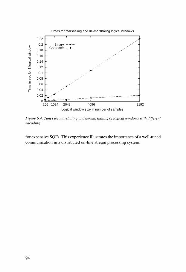
0
0.02
0.04
0.06
0.08
0.1
0.12
0.14
0.16
0.18
0.2
0.22
8192 4096 2048 1024 256
Tim
e in
sec
for
1 lo
gica
l win
dow
Logical window size in number of samples
Times for marshaling and de-marshaling logical windows
BinaryCharacter
Figure 6.4: Times for marshaling and de-marshaling of logical windows with differentencoding
for expensive SQFs. This experience illustrates the importance of a well-tunedcommunication in a distributed on-line stream processing system.
94

7. Continuous Queries in a ComputationalGrid Environment
In order to execute efficiently expensive continuous queries on high-volumedata streams, GSDM needs substantial computational resources. At the sametime, resource requirements are varying in time depending on the currentlyinstalled queries and their computational costs. The idea behind Grid middle-ware is to provide sharing of resources, such as computers, data, and instru-ments. In this chapter we investigate the possibilities to utilize computationalGrid resources on-demand for the needs of computationally expensive contin-uous queries.
7.1 Overview of GridsGrids [43, 33] enable sharing of distributed heterogeneous resources, such ascomputers, databases, and scientific instruments. The term Grid was chosenas an analogy to the electrical power grid that provides transparent, pervasiveaccess to electric power irrespective of its source. The purpose of computa-tional Grid middleware software is to provide an infrastructure where usershave transparent access to computing resources irrespectively of where thecomputing cycles are generated. This idea is a basis for computational mar-kets where service provides offer computational resources and users select aresource based on criteria including price and quality of service [65].
Several projects, such as Globus [35] and Nordugrid [61], provide tools forbuilding computational Grid infrastructures.
In a typical usage scenario the end users interact with the Grid middlewareby submitting requests, called jobs, for execution of an application programon some input data sets. In order to provide transparent execution of jobs, themiddleware software must provide capabilities for dynamic discovery, selec-tion, and allocation of grid-enabled resources. It also has to provide tools forjob description, staging the application executable, transferring the necessaryinput data files, submitting jobs to the resource’s management system, moni-toring the execution, and notifying the user and transferring the results whenthe job completes. In order to fulfill this role, Grid middleware needs to solvea number of problems. The main challenges are heterogeneity of resources
95

and technologies, scalability, multiple ownerships, preservation of autonomy,and dynamics.
Over time the Grid community realized that the required capabilities ofGrid middleware overlapped with the developments in the web services com-munity. As a result, a service-oriented architecture for the Grid was proposed,known as Open Grid Services Architecture (OGSA) [32]. Based on OGSA,the Grid middleware functionality is available through service description andinvocation standards of the web services community.
7.2 Integrating Databases and GridThe initial driving forces for the development of the Grid were in the areaof scientific and engineering applications. Data in these initial applicationswere organized as flat files and consequently the early Grid toolkits focusedon file support rather than management of structured data. As the file manage-ment systems and registries associated with Grid became complex, DBMSsstarted to be increasingly used to store the Grid meta-data. At the same timemore scientific applications emerged using the developments of, e.g., OO- andORDBMSs to organize their complex data. The requirement of scientific col-laboration created a need to be able to share such databases on the Grid.
In order to integrate databases with Grid infrastructure, Grid middlewarestack needs to include service-based interfaces to databases [65]. In manycases their functionality is similar to the existing database access interfacessuch as JDBC. However, more expressive interfaces are needed for request-response and publish-subscribe access to data.
Database technologies and Grid can mutually benefit of each other. Data-base management systems can benefit from unified access to computationaland storage resources, and from facilities for dynamic resource discovery andallocation. The Grid can benefit from database technology that provides theusers with data sharing, scalable management of large data sets, and declar-ative query languages. Data intensive tasks on Grid are typically specified asdirected acyclic graphs (DAGs) in terms of jobs, i.e. programs executed onfiles. A higher level abstractions are needed to ease the specification of Griddata-intensive tasks. Examples of projects that provide such abstraction areGridDB and OGSA-DQP [4].
7.3 GSDM as an Application for Computational GridsThe GSDM system can benefit from Grid facilities for dynamic resource dis-covery and allocation. The system has highly varying resource requirements.
96
When a new query is submitted, containing possibly expensive SQFs, thesystem needs to provide on-line execution with high throughput. It can beachieved by composing a parallel execution plan to run on newly incorporatedresources. When the query is stopped, the resource requirements of the systemdecrease correspondingly. Therefore, dedicating a fixed number of servers tothe system can lead to over-provisioning and inefficient resource utilizationin case the current load of the system is small. At the same time, the dedi-cated resources can still be insufficient to provide for an efficient execution ofvery expensive queries. Hence, this dynamics of resource requirements makesGSDM a good candidate for shared computational resources that are providedon-demand by a computational Grid infrastructure.
7.3.1 GSDM Requirements for GridsThe other side of the coin is the question how GSDM fits into the profile ofthe current computational Grid applications. In the following we analyze whatrequirements GSDM puts to a computational Grid and how they are fulfilledby the current Grid middleware.• Requirement I: High communication bandwidth to the processing nodes.
Traditionally database systems store high-volume data on disks. Hence,data locality is an important factor in query processing, in other words, itis preferable to perform the processing as close to data as possible to avoidtransferring of high-volume data. In a stream processing system wherestream data are not disk-stored, but communicated in real-time, this re-quirement changes. It is again favorable to process the stream data in prox-imity to the stream sources, but it is more important to use resources withhigh-bandwidth communication capacity for high-volume streams.
• Requirement II: Automatic staging of executables.GSDM is a main-memory database engine for stream processing and assuch it can be started by simply starting the executable with the initialdatabase image file. Therefore, in order to run the system on an arbitraryresource, staging of the executable is needed similarly to other Grid appli-cations.
• Requirement III: Support for parallel long-running jobs with guaranteedshort start-up time.Distributed execution plans for computationally expensive continuous queriesrequire multiple nodes to work simultaneously. Therefore, parallel jobsneed to be supported. CQs are also often long-running. At the same time,when a user submits a continuous query she expects short start-up time inorder to analyze the data currently produced by an instrument, sensor, etc.A start-up with an indeterminate delay means unprocessed stream data andmay lead to missed important discoveries.
97

• Requirement IV: IP Connectivity of individual computing nodes.Processed data are not locally stored on disks, but comes continuously fromexternal sources, such as instruments and software on the Internet. There-fore, individual computing nodes need to have IP addresses accessible fordata delivery from outside. Resources where all the communication goesthrough a single front-end node cannot manage high-volume streams com-munication.The above requirements are not completely satisfied by the current state of
computational Grids and Grid middleware. True staging of executables is notautomatically provided by the current Grid middleware. Consequently, today’sGrid applications are limited to use only Grid resources where the applicationexecutables have been prepared in advance, typically in a manual way.
Resource management of parallel computing resources is typically per-formed by batch-oriented systems, such as PBS for cluster computers. Whena job is submitted, the batch system puts it to a batch queue according to job’spriority and schedules it following some resource management policy. As aresult the job might wait long before the resources are allocated for it. Corre-spondingly, the job submission using Grid middleware is batch oriented withunpredictable waiting times.
The resource management systems of clusters often dedicate parts of theresources for interactive remote-session jobs for the purposes of applicationdevelopment and testing. These interactive jobs have typically short start-uptimes and it is possible to acquire several nodes at once as long as there areresources available. Interactive jobs (rather than batch jobs) could be used forservicing GSDM queries because of their short start-up times. However, clus-ter’s resource managers often limit interactive jobs to be started only from theterminal sessions which prohibits programmatic startups. Furthermore, sincethe interactive jobs are not considered Grid production jobs, most Grid mid-dleware toolkits do not provide support for them.
Many computer resources accessible through the Grid infrastructure do notcurrently satisfy these requirements. At the same time the number of moni-toring applications processing streams increases and includes new domains.It is therefore desirable to consider the requirements of such applications forcomputational resources when new Grid-enabled computer resources are de-signed.
7.3.2 GSDM Resource AllocationIn a Grid environment the GSDM resource manager module in the coordinatorwould:1. Collect information about the status of the available cluster resources where
the GSDM executable is pre-installed. Of particular importance is the abil-
98

ity to get information about the approximate waiting time for the submittedjobs.
2. Select a cluster based on the expected number of available nodes and thewaiting time.
3. Submit a (interactive or batch) job to the cluster. The job contains a numberof nodes as a parameter. As a result a list of available computer nodes isprovided to other modules of the GSDM coordinator.
4. Multiple jobs can be submitted in a proactive way so that a minimum num-ber of nodes is always guaranteed.
7.3.3 Multiple Grid ResourcesIn the presented usage scenario a CQ runs on a single cluster computer. Wecan also consider an execution of a CQ distributed among several clusters.Using techniques from distributed databases, the CQ can be decomposed intoa number of continuous sub-queries assigned on different clusters based ontheir proximity to the stream sources. Such assignments would reduce thetotal communication traffic. Furthermore, the overall system efficiency canbe optimized by installing a new CQ on clusters where other queries alreadyprocess the same streams.
In order to implement such a scenario for processing distributed amongseveral clusters, a number of problems need to be addressed, for example:• CQ decomposition and site assignment need to take into account physical
proximity of stream sources and processing resources, as well as queriescurrently running in the system.
• Running on-line stream sub-queries on different clusters requires very strictsynchronization of resource allocation among clusters, which is currentlynot supported.
7.3.4 Grid Requirements for ApplicationsIn order to run GSDM as a Grid application, the system needs to conform toGrid standards and requirements, such as:• Authentication and Authorization. Users of Grids acquire resources through
a grid certificate schema. The Grid applications run while utilizing the cre-dentials of the user certificates, where the principle of a single sign-on isapplied. Hence, it is necessary to investigate a certificate utilization schemain order to run GSDM as a Grid application. For instance, the system canuse its own grid certificate, in which case the user interface needs to beaugmented with user authentication and authorization mechanism to en-sure that the system runs continuous queries only on behalf of authorizedGrid users.
99

• Security. Grid utilizes SSL protocol for secure communication. Hence, ac-commodation of this protocol might be required for communication ofcomponents of a distributed Grid application.
7.4 Related Projects on GridIn this section we present an overview of several database and stream process-ing projects utilizing Grid.
7.4.1 OGSA-DAIThe purpose of OGSA-DAI initiative [62] is to provide generic Grid dataservices for access to and integration of data held in relational DBMSs andin XML repositories, called data resource. A Grid Database Service (GDS)wraps a data resource and is capable of evaluating a collection of linked ac-tivities. The activities are one of the following kinds: database query, resulttransformation or result delivery. Thus, the project provides coarse-graineddatabase interfaces allowing for grouping database access, data transforma-tions and movement in a single request to the GDS.
OGSA-DAI addresses the problem for accessing stored collections of struc-tured and semi-structured data, while GSDM deals with the problem for on-line processing of streaming data sources under Grid.
7.4.2 OGSA-DQPOGSA-DQP [4] is a service-based distributed query processor for the Grid.It allows for declarative specification of complex applications accessing dis-tributed data sources and computational resources in a uniform way. Thus,OGSA-DQP provides functionality for declarative service orchestration com-plementary to work-flow systems. The system relies on OGSA services todynamically obtain the resources necessary for distributed query evaluation.OGSA-DQP adapts techniques from parallel databases to provide implicit par-allelism for computational tasks in data-intensive requests.
The architecture includes two services: Grid Distributed Query Service(GDQS) and Grid Query Evaluation Service (GQES) whose functionality re-sembles GSDM coordinator and working nodes. The GDQS compiles, opti-mizes, partitions, and schedules distributed execution plans over multiple exe-cution nodes. It interacts with the appropriate grid registries to obtain metadataabout the data sources and computational resources. When a distributed queryis posted to the system, the query evaluation system is dynamically composedfrom a number of GQES services. They are the execution nodes in the distrib-uted query plan.
100

The OGSA-DQP is oriented for application that query high-volume storeddata in science and medicine. The query processing utilizes iterative modelcombining push and pull-based interface between query execution modules.By contrast, we target on-line stream processing applications and utilize data-driven (i.e. push-based) data flow processing model.
OGSA-DQP re-uses the optimization, partitioning, and scheduling capabil-ities of Polar* engine [77] and re-implements the query execution engine ina service setting. It uses OGSA Grid Data Service that ensures that metadataand data are accessed via a standard well-defined interface. It also uses OGSAservices for data transport and authentication.
Since the current Grid middleware does not support true application stag-ing, OGSA-DQP assumes pre-installation of services software on the requiredGrid nodes. The service-based system architecture is used to guarantee timelyacquisition of resources for the query execution, i.e. GDQS service providerseither have themselves enough resources or have service level agreementswith other GDS providers and computational resource providers that hostquery evaluation services. Therefore, the functionality of OGSA-DQP requiresQoS guarantees for the participating in the distributed plans Grid data servicesand web services. Computational resource discovery is not automatically pro-vided but partially supported via querying indexing services about the set ofresources specified by the user.
GDQS coordinates between the query optimizer and GQES instances ex-ecuting the distributed plan similarly to the GSDM coordinator controllingthe working nodes. In both cases a distributed query evaluation system isconstructed on the fly. However, OGSA-DQP has loosely-coupled service-based architecture, while GSDM is a tightly-coupled system. One of the placeswhere this difference is noticeable is the communication between the systemcomponents. One of the reported OGSA-DQP performance bottlenecks is thelack of an efficient data transfer mechanism. Currently the data transport ser-vice provides for transfer of XML documents over SOAP/HTTP. High-volumestreams of scientific data require efficient communication. Having the inter-GSDM communication under our control allowed to optimize it to an accept-able level where the communication is not a bottleneck.
Resource selection and scheduling algorithm that enables partitioned (intra-operator) parallelism for distributed query execution in a Grid environment ispresented in [38]. The algorithm starts with a valid query plan with mini-mum partitioned parallelism and in each step finds the most costly operatorfor which there are available machines, increases the parallelism by one de-gree for this operator by allocating an available machine, and assesses theperformance using a well-defined cost model. The algorithm stops when per-formance improvement is bellow a certain threshold.
We use a similar idea to create parallel plans with different degrees of par-
101

allelism. However, we utilize training mode to find an optimized data flowsince we cannot rely on precise cost model for an extensible system with user-defined functions running in a heterogeneous environment.
The OGSA-DQP optimizer achieves partitioned parallelism using the ex-change operator with pre-defined partitioning method. By contrast, we pro-vide customizable partitioning and also a user-defined partitioning, includingwindow split as a form of intra-object partitioning for intra-function paral-lelism.
Recent work [37] addresses the need for generic adaptivity framework forGrid query processing and proposes plan adaptation by changing the degreeof parallelism and the distribution vector to balance the load among heteroge-neous resources.
7.4.3 GATESGATES (Grid-based AdapTive Execution on Streams) [23, 24] is a Grid mid-dleware system aimed for distributed processing of high-volume data streams.It is designed to use the existing Grid standards and tools to the extent possibleand is build on OGSA standard and Globus Toolkit 3.0 middleware. The sys-tem provides users with a high-level interface to specify algorithms for datastream processing. Another important aspect of the system is its ability toadapt the processing to achieve the best possible accuracy while maintainingthe real-time constraint on the analysis.
The application developer divides the application into stages, implementsthe processing in each stage, and chooses one or more adjustment parame-ters. The adjustment parameters provide adaptivity, e.g. allow to increase theprocessing rate in order to achieve real-time processing at the price of reducedaccuracy. The application starts using an XML configuration file that describesthe application stages and their locality. The execution is performed through anumber of communicating GATES Grid services that are able to contain andexecute user-specified code and implement a self-adaptation algorithm.
The GATES Grid services resemble the GSDM working nodes in the sensethat both are distributed execution components for stream processing startedon-demand and customizable by uploading of user-defined code and SQFs.The difference is in the level of abstraction and flexibility provided. GATESapplication stages are fixed and pre-defined pieces of code created by theapplication developer and stored in a configuration file. In GSDM the userspecifies continuous queries in terms of declarative SQFs and the coordinatorcreates dynamically a distributed execution plan.
The GATES system is designed for applications with expected high-volumecommunication and relatively cheap computations. Hence, the work focuseson a resource allocation algorithm minimizing the communication costs be-
102

tween the nodes, while parallel processing of expensive operators on a singlestream is not considered at all. The distributed pattern of execution is limitedto multiple input streams of the same type that undergo the same chain ofoperations, and are merged in the later stages of the application. We providehigh-level and general framework for specifying distributed patterns throughthe data flow distribution templates.
Similarly to other Grid applications, GATES project intends to use the in-formation services provided by Grid middleware for resource discovery. How-ever, the problem how to simultaneously and with short start-up time allocatemultiple Grid resources needed for distributed stream processing is not ad-dressed.
7.4.4 R-GMAR-GMA (Relational Grid Monitoring Architecture) [66] is a data integrationsystem for Grid monitoring. It allows for publication of both static and dy-namic stream data as well as specifying of continuous, history and latest-state queries. The system utilizes “local as view” approach for data integrationthrough a global relational schema, providing a global view over different Gridresources, and local data sources whose schemas are views defined over theglobal schema. The requests for monitoring information are specified in SQL.
Monitoring information about dynamic characteristics of Grid resources isprovided as data streams from information providers to the information con-sumers. Stream republishers aggregate streams from other providers usingspecifications in SQL. By constructing a hierarchy of stream republishers andusing a DBMS for the latest stream values, the system allows more complexprocessing including joining and aggregating of latest stream values.
The design of the system is oriented very much to providing scalability, per-formance, and integration to handle the large amounts highly-distributed Gridmonitoring data. However, the volume of the stream data is much lower thanthe volume of a scientific instrument stream, e.g. one data sample is generatedevery 30 sec, and consequently the problem how to distribute a high-volumestream for efficient parallel processing is not relevant in this context.
103

8. Related work
This chapter presents an overview of research projects related to the GSDMsystem. GSDM is a prototype of data stream management system and thus wepresent other DSMSs related to GSDM with respect to stream data modeling,query languages for continuous queries, processors for continuous queries,distributed processing of streams, and data stream partitioning strategies. Inthe first section we describe the related DSMS projects and how GSDM differsfrom them.
The next sections present other technology related to GSDM, namely, con-tinuous query systems operating on stored data, parallel DBMSs providingscalable processing of non-stream data, and DBMSs used for managementand analysis of scientific data.
8.1 Data Stream Management SystemsDuring the last years data stream processing has been an active area of researchfor the database community and many projects and prototypes of DSMSs havebeen developed and published in the literature. The earlier systems typicallyhave central architecture where continuous queries are processed on a cen-tral server over possibly distributed stream sources. The DSMSs with centralarchitecture are related to GSDM with respect to data modeling, query lan-guages, and query processors for continuous queries.
Over the last three years many DSMSs were augmented with distributedand parallel processing capabilities. This capabilities are more closely re-lated to GSDM with respect to problems such as data partitioning, distributingthe continuous query processing among multiple nodes, and load balancing.When we describe such systems we start first with central architecture beforepresenting the distributed and parallel extensions.
Most of the stream processing systems [17, 27, 57, 59, 81], including dis-tributed ones, have fine granularity of stream data items and relatively smallcost of the stream operators per item. Hence, the distributed extensions oftenaddress the problem of an optimal operator distribution that achieves goodload balancing among the machines. In contrast, the streams in the scientificapplications we address have big total volume and data item size, and the user-defined functions are computationally expensive. Therefore, we address the
105

problem for scalable execution of expensive stream operators (SQFs) throughparameterizable templates for partitioned parallelism.
8.1.1 AuroraAurora [17, 2, 14] is a stream processing engine with central architecture de-veloped at Brown, Brandies, and MIT. It is a data-flow system where queriesare composed utilizing a boxes and arrows paradigm from process flow andwork flow systems. Data sources, such as programs or hardware sensors, gen-erate streams that are collections of data values with fixed schema containingstandard data types. The output streams are presented to applications, whichare designed to deal with asynchronous data delivery.
The Aurora model is based on an extension of the relational model wherestream data are of standard relational atomic data types. The cost of the op-erators is relatively small, so that the system has to schedule efficiently cen-tralized processing of units with fine granularity. In contrast, we address par-allel processing of computationally expensive stream operators utilizing user-defined partitioning of streams that may contain data of complex user-definedtypes.
A distinguishing feature of Aurora is the quality of service (QoS) supportthat is an integrated part of the system design. A number of convex QoS graphscan be provided by an application administrator for each result stream. Thegraphs specify utility of the result in terms of performance or quality metricssuch as delay, percentage of dropped tuples, or result values. Scheduling al-gorithms utilize the QoS graphs and aim at optimizing the overall utility ofthe system.
Aurora’s continuous queries are specified in a procedural way using a GUI.It is possible to combine multiple continuous queries, eventually for differentapplications, into one so-called query network. Thus, shared processing ofCQs is supported given a specification by the application administrators.
No arrival order is assumed in Aurora’s data model. Hence, order-sensitiveoperators are designed to handle this by either ignoring tuples out of orderor introducing a slack specification, where the slack is a fixed number of tol-erated out-of-order tuples. By tolerating partial disorder the system can giveprocessing priority to tuples that contribute higher QoS utility.
The last overview of the project in [14] indicates the need for supportingdifferent feed formats for input streams. The suggested design solution is toprovide special input and output converter boxes that are dynamically linkedinto the Aurora process. These boxes are similar in functionality to the GSDMstream interfaces but we go further by also encapsulating in them networkcommunication of streams. Other lessons from the Aurora experience are theneed for global accessibility to the meta-data and a programmatic interface, al-
106

lowing to script the query network. These features are available in GSDM. Forexample, the coordinator creates dynamically the installation scripts to be sentto the working nodes in order to install the distributed query execution plan.
8.1.2 Aurora*, Medusa, and BorealisTwo proposals to extend the Aurora stream processing engine for a distributedenvironment were presented in [25], followed by the work on Borealis [1] asa second generation stream processing engine.
In Aurora* multiple single-node Aurora servers belonging to the same ad-ministrative domain cooperate to run an Aurora query network. Medusa is adistributed infrastructure for service delivery among autonomous participantswhere participant collaborations are regulated using economic principles, e.g.,pair-wise contracts to specify a compensation for each service.
Scalable communication infrastructure is proposed using mechanisms forglobal name space and discovery, routing, and message transport. To providescalable inter-node communication, streams are multiplexed to a single TCPconnection. A message scheduler implements a policy for connection sharingbased on QoS specifications. By contrast, in GSDM we use one TCP con-nection to implement an inter-GSDM stream. This choice is justified by thecharacteristics of the GSDM applications: high volume of data in a singlestream and the coarse granularity of the expensive user-defined functions.
The Aurora* proposal includes dynamic adjustment of processing alloca-tion among the participating nodes. Transformations of the query network arebased on a stop-drain-restart model. Two basic mechanisms for load sharingamong the nodes are proposed: box sliding and box splitting. Box sliding al-lows boxes on the edge of a sub-network on one machine to be moved to theneighbor, thus reducing the load and possibly the communication.
Box splitting creates a copy of a box intended to run on another machine. Inorder for a box to be split it must be preceded by a filter box with a predicatethat partitions the input stream and be followed by one or more merging boxes.The merging boxes depend on the predicate in the filter box as well as on thesemantics of the box to be split.
The proposed concept of box splitting has some similarities to our templatefor partitioned parallel execution of SQFs. The Aurora* authors point out thechallenges related with the choice of a filter predicate for stream partitioningand the determination of appropriate merging boxes. However, the work doesnot address the problem of how to automatically create filtering and merg-ing boxes for a given box splitting, which we provide through customizabletemplates. The ideas in [25] are presented at a proposal level and neither animplementation nor experimental results on box splitting are reported in thefollow-up literature.
107

Borealis [1] is a proposal for a second generation stream processing enginethat inherits core stream functionality from Aurora and distribution function-ality from Medusa. It extends Aurora with support for dynamic revision ofquery results, dynamic query modifications, and a scalable multi-level opti-mization framework that strives to incorporate sensor networks with streamprocessing servers.
Recent work focus on two problems of distributed stream processing: loadbalancing [88] and fault-tolerance [15]. Since the target applications involvebig numbers of relatively cheap stream operators, the load balancing prob-lem consists of good distribution of operators among the nodes. The initialdistribution of a query network utilizes localities of stored data and statisticsobtained through trial runs. Further re-distribution is achieved dynamicallythrough box sliding and correlation-based peer-wise or global re-distributionalgorithms [88].
Several strategies for providing fault tolerance are presented in [15]. Be-sides adapting the standard active and passive stand-by approaches to thestream processing context, in upstream backup each server acts effectivelyas a back-up server for its downstream servers. The fault tolerance problemsare not addressed currently in GSDM; this research is complementary to ourwork and its results can be utilized in a future work.
8.1.3 Telegraph and TelegraphCQThe goal of the Telegraph project at UC Berkeley is the development of anadaptive data flow architecture. The Telegraph architecture includes three typesof modules: query processing modules which are pipelined non-blocking ver-sions of the standard relational algebra operators such as select, join, groupetc.; adaptive routing modules, such as eddy [8], which are able to re-optimizethe query plan while a query is running; and ingress and caching moduleswhich are wrappers providing interface to external data sources. All the mod-ules communicate through an inter-module communication API called fjords.
Two prototypes, CACQ [57] and PSoup [20], extend Telegraph with ca-pabilities for shared processing over streams. In CACQ, standing for continu-ously adaptive continuous queries, an eddy can execute a “super”-query corre-sponding to the disjunction of all the individual continuous queries. Each tuplemaintains an extra-state that serves to determine which queries should obtaina result tuple. In order to optimize selections for shared execution, a groupedfilter operator is introduced that indexes predicates over the same attribute.PSoup extends the mechanisms developed in CACQ by allowing queries toaccess historical data and supporting disconnected operation where users canregister queries and return intermittently to retrieve the latest results.
The goal of TelegraphCQ [19, 49] is shared, continuous data flow process-
108

ing with emphasis on adaptability. It is a result of redesign and re-implementa-tion of Telegraph based on PostgreSQL that also uses the experiences fromCACQ and PSoup.
As a part of TelegraphCQ a flux operator [75, 74] has been designed to pro-vide partitioned parallelism, adaptive load-balancing, high availability, andfault tolerance. The first version of flux [75] provides adaptive partitioning onthe fly for optimal load balancing of parallel CQ processing. General parti-tioning strategies, such as hash partitioning, are encapsulated in the flux oper-ator. We also have a customized general partitioning and in addition handleoperator-dependent window split strategies customizable with user-definedpartitioning for scalable execution of expensive stream operators.
The main advantage of flux is the adaptivity allowing for data re-partitioning.One of the motivations is the fact that content-sensitive partitioning schemasas hashing can cause big data skew in the partitions and therefore need loadbalancing. We do not deal with load imbalance problems since the partitioningschemas we consider (window split with user-defined partitioning and win-dow distribute with Round Robin), chosen to meet our scientific applicationrequirements, are content insensitive, i.e. do not cause load imbalance in ahomogeneous cluster environment.
The last version of flux [74] encapsulates fault-tolerance logic that allowsfor constructing highly-available parallel data flows. The techniques involvesreplicated computations and mechanisms for restoring failured operators statesand lost in-flight data. This work is complementary to the problems of user-defined stream partitioning presented here.
Queries in TelegraphCQ can be specified on both static and streamed data.For each stream there is a user-defined wrapper consisting of init, next, anddone functions that are registered to the system. GSDM stream interfaces pro-vide similar functionality. However, by utilizing object-relational modelingwe put stream sources in a type hierarchy and associate the stream interfaceswith stream types rather than with individual stream source. Thus, we allowto have more than one stream source using the same stream interface. Further-more, we provide for multiple interfaces for the same stream type, so that datacan be fed into the system using different communication media.
Modules in Telegraph communicate through the fjords API [56] that sup-ports both push and pull connections and thereby is able to execute queryplans over a combination of static and streaming data sources. In the currentimplementation GSDM does not provide pull-based communication betweenworking nodes. However, stream query functions can access locally stored sta-tic data in a pull-based manner through the generic capabilities of the Amos IIquery processor.
109

8.1.4 CAPEContinuous Adaptive Query Processing Engine, CAPE [70, 71], is a pro-totype system developed at Worcester Polytechnic Institute. D-CAPE [52]is a distributed stream processing framework based on CAPE and designedfor shared-nothing architecture. The system is designed for highly dynamicstream environments and employs an optimization framework with heteroge-neous-grained adaptivity. CAPE focuses on precise results computation byemploying different optimizations and does not consider load shedding andapproximation of results. CAPE utilizes punctuations [86] that are dynamicmeta-data used to model static and dynamic constraints in the stream context.The punctuations can be exploited to reduce resource requirements and to im-prove the response time. Stream tuples and punctuations are assumed to beglobally ordered on their timestamps recording their arrival time.
Fine-grained adaptivity is achieved by reactive query operators whose exe-cution logic can react to the varying stream environment. An adaptive schedul-ing framework selects one algorithm from a pool of scheduling algorithms thatbest fits to the optimization goal defined as a quality of service specificationcombining multiple metrics. Online re-optimization and plan migration re-structure the query plan at runtime including plans with stateful operators. Anadaptive distribution framework allows to balance the workload among a clus-ter of machines and maximally exploit available CPU and memory resources.Adaptations at all levels are synchronized and invoked with different frequen-cies and under different conditions, where the adaption intervals increase fromoperator-level to the distributed processing level.
D-CAPEIn D-CAPE a number of CAPE engines perform distributed query process-ing and one or more Distribution Manager monitor the execution and initiatere-distribution when needed. Run-time statistics is periodically obtained andused to assess the processors’ workload and to decide about re-allocation.A connection manager module communicates with the processors to estab-lish operators to be executed. A distribution decision maker decides how todistribute the query plans using a repository of distribution patterns. Exam-ples of distribution patterns are Round Robin, which tries to fairly assignequal number of operators to each processor, and grouping distribution, whichtries to minimize network connections by keeping adjacent operators on thesame processor.
D-CAPE monitors query performance and redistributes operators at run-time across a cluster of processors. The redistribution tries to alleviate themost-loaded machines. The algorithm that picks operators to be moved givespreferences to operators that would remove network connections in the over-all distribution.
110

The components of the distributed GSDM architecture resembles those inthe D-CAPE architecture. The GSDM coordinator functionality is performedby the CAPE distribution manager in sense of generating distributed plans,installing plans on the query processing engines, and monitoring the execu-tion. D-CAPE’s repository of distribution patterns is similar to the GSDM’slibrary of distribution templates, which in both projects guide the generationof distributed plans.
D-CAPE’s distribution patterns allow for various types of parallelism oninter-query, intra-query, and intra-operator level. Partitioned parallelism, asused in flux [75] and Volcano [39], is applied to query operators with largestates accumulated at run time, such as multi-way joins. By contrast, we focuson partitioned parallelism for computationally expensive user-defined opera-tors (SQFs). Our generic distribution template for partitioned parallelism isparameterizable with a user-defined partitioning strategy providing for intra-object parallelism of user-defined operators.
As in D-CAPE the GSDM architecture allows for re-optimizing parallelplans, though this functionality is not implemented in the current prototype.The statistics collector at the coordinator periodically gathers informationabout the cost of SQFs and communication at working nodes that allows toassess the workload.
The redistribution opportunities for plans with partitioned parallel execu-tion of expensive operators in GSDM are somewhat limited in comparison to ageneral distribution framework. For example, the operator-level redistribution[52] assumes that an operator is small enough to fit on one machine. Hence,our vision about the changes that are appropriate in GSDM’s partitioned par-allel plans includes replacement of the partitioning strategy or increase of thedegree of parallelism given an ability for additional resource allocation on-demand. The problems related with the dynamic re-optimization of parallelpartitioned plans are subject of future work.
8.1.5 Distributed Eddies
The work on distributed eddies [85] puts adaptive stream processing in a dis-tributed environment. An eddy [8] is a tuple router at the center of a dataflow that intercepts all incoming and outgoing tuples between operators inthe query plan. Eddies collect execution statistics used when the routing deci-sions are made. With distributed eddies each operator in the distributed plan isaugmented with eddy’s functionality, i.e. makes routing decisions and collectsand exchanges statistics with other operators. An analytical model for a dis-tributed query plan is constructed using a queuing network. Two performancemetrics are defined, the average response time (latency) and maximum data
111

rate. An optimal routing using the queuing network model is computed andsix practical routing policies are designed and evaluated through simulation.
The ideas of box splitting and sliding suggested in Aurora* are used todynamically reallocate resources among operators so that more expensive op-erators can get more resources when needed. As we discuss, box splittingis a form of parallel processing where data partitioning among the operatorinstances is done as a part of the applied tuple routing policy. The policiesare implemented as weighted distribution vectors. Such parallel processing issimilar to our window distribute, but we customize explicitly the data parti-tioning strategy. Furthermore, we also provide order preservation of the resultstream while distributed eddies do not guarantee that the result tuples wouldbe ordered at the receiving sink. Finally, the GSDM window split partitioningof big stream data items does not have analogue.
Future work will investigate the application of the analytical queuing net-work model for generation and optimization of parallel execution plans inGSDM. For example, one possibility is to use the model to compute the ex-pected latency or throughput with different partitioning strategies. However,several limitations restrain a direct application of the model to parallel execu-tion plans in GSDM. For example, the assumption about well-known costs ofthe operators in the plan does not hold in an extensible system, such as GSDM,where the costs of user-defined functions over user-defined data types mightbe hard to define or obtain from the authors of the code. Hence, we need someform of test runs of plans for statistics collection purposes.
8.1.6 Tribeca
Tribeca [81] is an extensible stream database system designed to support net-work traffic analysis. The system uses a data flow query language where userscan explicitly specify how the data flows from one operator to another. TheTribeca queries have a single source stream and one or more result streams.Hence, Tribeca is one of the first systems that practically support shared ex-ecution of analyses over the same input stream. The operators include quali-fications (filters), projections, aggregates, demultiplexing (demux) and remul-tiplexing (mux). Demultiplexing partitions a stream into sub-streams basedon the data content similarly to GROUP BY clause in SQL. Remultiplexingis used to combine the logical sub-streams produced by demux or unrelatedstreams of the same data type similarly to union operator in the relationalalgebra. It is not reported whether mux takes care to preserve the orderingof elements. Tribeca also supports windows on streams and a limited formof join.
Tribeca queries are compiled and optimized using many of the traditional
112

relational optimizations. The queries have pipelined execution and intermedi-ate results are never unnecessarily materialized.
In GSDM stream partitioning and combining SQFs in the window distributestrategy are similar to Tribeca’s demux and mux operators. However, Tribeca’spartitioning is based only on data content and performed for aggregation pur-poses in a centralized architecture, while in GSDM user-defined partitioningis used for parallelization. Tribeca has a central architecture and queries arelimited to run over a single data stream. GSDM uses a distributed architecturefor parallel execution and allows for specifying data flow graphs with multipleinput streams.
8.1.7 STREAMSTREAM [10, 59, 6] is a general-purpose prototype of relational-based datastream management system developed at Stanford University. The projectproposes a declarative query language for continuous queries and focuseson problems such as adaptivity, approximation, and scheduling in a centralprocessing architecture.
In [6] an abstract semantics for continuous queries is defined and imple-mented in CQL, a declarative query language extending SQL with windowspecifications from SQL-99. Queries can be specified on both streams andrelations defined using a discrete, ordered time domain. The declarative con-tinuous queries are compiled into a query plan composed of operators, queuesbuffering tuples between operators, and synopses that store the operator state.The operators belong to one of the classes relation-to-relation, stream-to-rela-tion, or relation-to-stream. Stream-to-relation operators are based on the con-cept of a sliding window over a stream and expressed using a window speci-fication, such as [Rows n] for count-based windows, and [Range t] fortime-based windows.
The system has an adaptive query processing infrastructure that includesalgorithms for adaptive ordering of pipelined filters and pipelined multiwaystream joins [12]. In the area of operator scheduling STREAM uses a chainscheduling algorithm [9] to minimize runtime memory usage. When the loadexceed the available system resources, STREAM provides approximate an-swers of continuous queries [59]. If the CPU time is not sufficient, samplingoperators are introduced in the query plan that probabilistically drop elementsand thus save CPU time. In the case of limited memory the approximation canbe achieved by reducing the size of synopses, maintaining a synopsis sample,using histograms or wavelets, etc.
If the resources of a central system are not sufficient, STREAM addressesthe problem by approximate query answering. In contrast, in GSDM we con-sider instead parallel execution of expensive stream operators. We do not ad-
113

dress problems of scheduling of many cheap operators or adaptive reorderingof query plans and, thus, the work on STREAM is complementary to ours.
The problems of time management in data stream systems are addressedin [79]. The query processor of a DSMS usually needs to process elementsin increasing time stamp order to provide semantic correctness of continuousqueries. However, when time stamps are put at multiple distributed streamsources, the arrival order of the elements at the DSMS may differ from theincreasing application time stamp order. The problem of synchronization ofunordered distributed streams is solved by an input manager that buffers out-of-order stream elements and presents them ordered to the query processorthrough a mechanism, called heartbeats. The heartbeats are as a special kindof punctuations that guarantee that all the future elements on streams willhave timestamps bigger than the heartbeat. The proposed algorithm for heart-beats generation models factors influencing the synchronization of distributedstreams, such as application time skew and network latency and can be appliedin future work in GSDM for synchronizing distributed application streams.
8.1.8 GigascopeGigascope [27] is a high-speed stream database specialized for IP networkmonitoring applications. The Gigascope query language, GSQL, provides toolsto define declarative SQL-like queries and to compose them into a more com-plex processing chain. It is a pure stream query language, i.e. all inputs andthe output of a GSQL query are data streams. The basic supported streamoperators are selection, join, aggregation, and stream merge. Gigascope is anextensible systems where user-defined functions can be registered in a func-tion registry and called in the queries. In this way Gigascope supports high-performance specialized algorithms for network analysis. Similarly we sup-port user-defined scientific operations, e.g. FFT, for the space physics streamapplications.
Gigascope has a two-level query architecture optimized for the networkanalysis applications. Low level queries (LLQs) access source streams and areintended for data reduction. High level queries (HLQ) perform more complexprocessing. When a GSQL query is defined over source streams, Gigascopecreates one LLQ for every source stream and transforms the original queryinto a HLQ executing over the output streams of LLQs.
Furthermore, GSQL allows the user to associate a name with a query, whichis used to access the query result stream from an application or an anotherGSQL query. In this way GSQL queries can compose more complex process-ing chains. In terms of GSDM, the named GSQL queries correspond to de-fined SQFs without parameters. In GSQL the name of the query identifiesthe result stream, but in order to specify a similar query over another source
114

stream, the user must define and name a separate query. The LLQs allow non-stream parameters to be defined and bound during the query instantiation.
By contrast, SQFs in GSDM are parameterized on the input streams andeventually other parameters. This allows compact parameterized specificationof complex distributed processing, e.g. an SQF that is a template parameteris instantiated automatically by the template constructor, which may includemultiple instantiations on different input streams. Due to the parameteriza-tion, the name of an SQF cannot identify the result stream, but instead systemgenerated stream identifiers are used.
The GSQL processor generates C and C++ code implementing the queries.LLQs are linked into the stream manager, while HLQs run as separate processesand communicate data through shared memory. Depending on the capabilitiesof the computer’s network interface card (NIC), some LLQs in Gigascope canexecute inside the NIC. In contrast, the query executor in GSDM runs SQFsalways inside of a working node following a scheduling policy.
Even though the query execution in Gigascope is composed by a streammanager and a number of high level query processes, the architecture is de-signed to run on a dual CPU server with shared memory communication be-tween processes. By contrast, we address distributed and parallel executionwith potentially high degree of parallelism in a shared-nothing architecture.
In order to bound the state of the stateful operators, such as join and ag-gregation, Gigascope uses ordering properties of the streams and predicates inthe query specification instead of explicit definition of sliding windows com-monly used in other projects. For example a join window is determined by ajoin predicate on the ordering attributes on each of the joined streams. Thisapproach fits better the specifics of network data streams that often containseveral timestamps and sequence numbers.
The merge operator in Gigascope is similar to our S-Merge operator. Inorder to handle the danger of blocking in the absence of tuples on some of theinput streams, Gigascope injects ordering update tokens into the data stream.Instead, we use a time-out parameter of S-Merge.
8.1.9 StreamGlobeStreamGlobe [51] is a prototype for distributed stream processing in a peer-to-peer infrastructure developed at Munich Technical University. XML datastreams are queried through a windowed extention of XQuery supportingcurrently selection, projection, aggregation, and user-defined operations. Themain focus is multi-subscription optimization where queries over the samestream source and with overlapping predicates share computation by sub-sumption. As a result of sharing the network traffic and computational loadis reduced.
115

The system architecture is implemented based on OGSA where componentsare collaborating Grid services. The services are available according to thecapabilities of the peers.
Continuous queries are distributedly executed given that the result streamsof other queries can be used. The queries without overlap with other queriesare executed in a centralized manner. By contrast, GSDM focuses on paral-lel execution of queries with expensive user-defined functions, which is notconsidered in StreamGlobe.
8.1.10 Sensor Networks
A number of DSMSs are oriented to process streams generated by sensor net-works [16, 56, 28]. Typically, a large number of small-scale sensors, con-nected through a wireless communication interface, are sensing and transmit-ting relatively simple data units, such as temperature or pressure measure-ments. Since the conservation of battery power is a major concern, work in[89] proposes efficient in-network query processing capable for trading-offcostly communication for cheap local computations. By contrast, scientificinstruments in the GSDM target applications generate enormous amount ofnumerical data and we focus on scalable computations through parallelism.
Nile [41] is a prototype of a stream processing engine developed at Pur-due University. It extends an object-relational DBMS, Predator, with capabil-ities to process continuous queries over data streams. Similarly to GSDM,stream data sources are modeled by a stream type and data are retrievedthrough stream type interfaces. Queries are specified in an extension of SQL.The work focuses on providing windowed operators and in particular on thein-ordered execution of time-based window joins. In contrast to GSDM, thequery processing is performed on a centralized architecture.
More recent work on Nile-PDT [3] introduces an abstract data type to rep-resent multiple streams in sensor networks. A specialized operator Sensor Net-work Join (SN-join) produces pairs of matching sensor streams based on somesimilarity metric. SN-scan operator attaches the sensor network platform to thequery processing system and provides load shedding by more rare processingof sensors that do not contribute to the final results of the query oriented tophenomena detection. The operators provide relevance feedback to their pre-decessors that guides the predecessors in giving preferences to some of theinput streams. In this way an utility-based data shedding is used to handleoverload situations for centralized processing of sensor network streams. Bycontrast, we focus on scalable processing through parallelism and do not ad-dress data shedding.
116
8.2 Continuous Query SystemsThe concept of continuous queries was first introduced in [84] to name queriesthat are issued once and run continuously. In this work an incremental evalua-tion approach is used to avoid repetitive computations over append-only datasources.
NiagaraCQ [22], developed at University of Wisconsin, supports scalablecontinuous query processing over multiple, distributed XML files. It utilizesgrouping of queries based on their similarities, which leads to several bene-fits, such as shared computations and reduced number of query invocations.The group optimization is incremental, i.e. new queries are added to existingquery groups without having to regroup already installed queries. Incrementalevaluation of CQs is provided by considering only the changed portion of theupdated XML files.
Continuous query processing of stored data in NiagaraCQ is triggered usingan event detector that detects timer events for timer-based queries and changesof files for change-based queries. By contrast, on-line stream processing sys-tems, such as GSDM, typically require an active scheduling mechanism thatschedules continuous queries whenever new data has come and there are avail-able processing resources, rather than waiting for a triggering event.
NiagaraCQ uses a centralized architecture for shared processing of rela-tively simple continuous queries over distributed XML files. In contrast GSDMhas a distributed architecture to achieve scalable on-line stream processing in-volving expensive SQFs.
8.3 Database Technology for Scientific ApplicationsScientific applications are characterized by high volumes of data with typi-cally complex structure and non-trivial operations. Hence, they put require-ments for database technology that are not met well by the main-stream rela-tional databases oriented to business application. Therefore, scientific appli-cations were one of the major driving forces for the development of object-oriented and object-relational DBMSs. The current ORDBMS allow for betterrepresentation of scientific data by ability to extend the type system with newbase types and complex user-defined types together with user-defined opera-tions over them.
The work in [87] proposes the idea to extend the concept of a database querywith numerical computations over scientific data, and the query optimizer withtransformation and implementation rules applicable to these operations. Thefocal point are the advantages that the algebraic database query optimizationcan provide to the scientific computations. In contrast to our work, the paper
117

does not consider on-line stream processing and assumes centralized architec-ture.
The work points out important observations concerning the requirementsof scientific applications for database query processing. For instance, morediverse implementation techniques are available for scientific computationsoptimization criteria must be extended with numerical accuracy and stability.In scientific computations CPU costs are much more varied than in relationalqueries and often dominate the cost of specific operators (opposite to I/O costin traditional RDBMS). Therefore, the extensibility of the system is very im-portant so that the optimizer can utilize user-defined transformation rules andcost models. We go a step further by providing a generic mechanism to ex-tend the system with user-defined partitioning utilizing semantics of scientificcomputations for scalable parallel execution.
8.4 Parallel DBMSData partitioning strategies for parallel databases [64] are well investigated forrelational databases. Strategies, such as Round Robin and hash partitioningcan be used as parameters of our window distribute strategy. What makes ourstream partitioning strategies different is that the processing must preserveordering of the stream. We provide this property by special stream operatorssynchronizing the parallel result streams in the combine phase.
The idea to separate parallel functionality from data partitioning seman-tics by customized partitioning functions is similar to Volcano’s [39] supportfunctions parameterizing the exchange operator. In contrast, we have pairs ofpartition and combine operators where the combine operator preserves thestream order. While window distribute parameterized by, e.g., Round Robin issimilar to the exchange operator, window split is novel.
RiverDQ [7] proposes a content-insensitive partitioning for load balanc-ing in heterogeneous execution environment. Currently, we focus on homo-geneous environments. Future work will investigate the possibilities to applyRiverDQ ideas in order to use GSDM on heterogeneous environments.
Data partitioning problems have been addressed in object-relational DBMSswith the purpose to achieve efficient parallel execution of UDFs while pre-serving their semantics [46, 60]. The work in [60] proposes a specification ofUDFs that allows generic parallelization and classifies the partitioning strate-gies for user-defined operations. It presents the generic pattern of partition,compute, and combine phases for UDFs. However, the idea to specify genericand modular data flow distribution patterns through templates is to the best ofour knowledge unique.
Even though the work in [60] is based upon the stream processing paradigm
118

for query execution, it differs from our work in the assumption that the dataare stored on disk and have limited size. This assumption allows for streamingthe data from the disk in different order as appropriate for the operations per-formed. In contrast, the on-line stream processing, including a parallel one,must conform to the ordering of the stream and cannot afford re-ordering forthe operator purposes since it is a blocking operation. Our window split forparallel execution of a UDF over a single logical window does not have ana-logue in [60].
119


9. Conclusions and Future Work
In this Thesis we presented the design, implementation, and evaluation of theGSDM prototype of an object-relational data stream management system forscientific applications.
The system provides users-scientist with tools to express complex analysesof streams, generated by instruments and simulators, as continuous queriescomposed of user-defined operations. A distributed and parallel architectureprovides for scalable execution of continuous queries with computationallyexpensive operations over high volume streams.
Using a generic framework the users can specify scalable parameterizeddistributed execution strategies by the means of data flow distribution tem-plates. Several common distribution patterns are available through a built-inlibrary of templates. Using the library we define a generic template for parti-tioned parallelism, PCC.
We defined two overall parameterizable parallel strategies: the so-calledwindow split that divides a stream data items (logical window) into sub-win-dows to be processed in parallel by the partitions, and window distribute thatdistributes several logical windows among parallel partitions. Window splitprovides for intra-object parallel execution of user-defined functions, whilewindow distribute provides for inter-object parallelism. Both overall strategiesare customizable with different partitioning methods in order to instantiatea particular stream partitioning strategy. Through the customization windowsplit has knowledge about the semantics of a user-defined function to be par-allelized for the purposes of more efficient execution. Our experiments showthat window split with user-defined partitioning of windows utilizing the se-mantics of the functions can achieve higher total throughput of the system inscenarios when expensive operations are executed on limited computationalresources.
Although the problem for parallelization of user-defined functions has beenaddressed in general in the literature about object-relational DBMSs, we arethe first to provide a generic mechanism for implementation of such parallelstrategies, as well as an experimental evaluation investigating the trade-offs ofthe two strategies.
We developed a basic optimization framework to provide parallel trans-parency to the user. Utilizing meta-data about valid partitioning strategies for
121

user-defined functions, the continuous query optimizer enumerates parallelplans and selects an optimized one using statistics collected from trial execu-tions.
We investigated the requirements for implementation of GSDM in a Grid-based environment.
GSDM is the first reported fully functional prototype for parallel process-ing of continuous queries. Leveraging upon an object-relational model, wemodel numerical data from scientific instruments as user-defined types andimplement operations over them as user-defined functions. Types of streamdata sources are organized in a hierarchy and inherit properties form a genericstream type. As part of the prototype implementation many software mod-ules have been designed, implemented, evaluated, and improved to a level offunctionality and performance that is acceptable with respect to the overallsystem performance and functionality. Among these are the continuous queryengine based on data-driven data flow paradigm, compiler of high-level CQspecifications into distributed execution plans, stream interfaces, inter-GSDMcommunication primitives, statistics collector for monitoring the execution,and protocols for installation, activation and termination of the CQ execu-tion in distributed environment. Our experiments with real scientific streamson a shared-nothing architecture show that in order for a distributed streamprocessing to be efficient, not only stream operators and scheduling inside ofa processing node, but also stream communication between nodes, need to becarefully designed and implemented.
Although in the work on the GSDM prototype we focus on the specificneeds of scientific applications, the system can be extended for other applica-tions with expensive operations over streams with complex and high volumecontent. For example, analysis of MPEG streams can be specified as CQ giveninterface implementation for this type of streams and operation implementa-tion to be plugged into the system.
The work on the GSDM prototype opens a number of interesting directionsfor future work. In the following we will enumerate some of them.
Shared execution of continuous queriesA number of work on continuous queries emphasize the need for shared ex-ecution of long-running CQ for the purposes of scalability and overall cost-efficiency of the systems. The proposed solutions [57, 22] utilize similaritiesin queries specifications and create shared execution plans by grouping pred-icates on a common attribute and evaluating simultaneously the predicatesin such groups. In the presence of expensive user-defined functions we canexpect even bigger benefit from shared execution of similar queries for theoverall system performance. It should be investigated how to share plans thatare graphs of user-defined functions.
122

Adaptive CQ ProcessingAdaptive query processing (AQP) [42, 11] interleaves query optimization andexecution, possibly multiple times over the running time of the query, in orderto adapt the processing to the changing execution conditions.
Long-running queries often experience during their life time changes inthe execution environment and characteristics of input streams. Hence, adap-tive execution of CQs is an important desirable property of CQ processing.A variety of adaptation techniques appeared recently in the literature span-ning from the operator-level adaptation, plan migration to another executionplan, changing the operator scheduling policy, or adapting distributed plans byre-distributing the load among the resources currently available [71, 12, 88].
Future work will investigate possibilities for adaptation of parallel execu-tion plans, such as changing the degree of parallelism and replacing one parti-tioning strategy with another. Such adaptation can response to changes in theavailable resources assuming relatively stable rates of streams generated byscientific instruments.
Integration with Grid InfrastructureThe ability of computational grids to provide computational resources on-demand can be very beneficial for GSDM running expensive CQs with vary-ing resource requirements. The current development of Grid middleware doesnot provide the resource allocation functionality as needed for the long-runningparallel GSDM jobs with guaranteed start-up time. Future work on this prob-lem depends on the future developments of the Grid middleware.
CQ OptimizationThe current optimization framework uses exhaustive parallel plan enumera-tion for an expensive SQF. To avoid generation and evaluation of possiblyvery big spaces of data flow graphs, the functionality of the optimizer needsto be enhanced with heuristics such as random walk or binary search of thesearch space.
Furthermore, methods for optimizing of CQs composed out of several SQFshave to be developed and evaluated. For example, investigating when it isworth to encapsulate a pipeline of two SQFs into one large SQF to be executedin parallel and when it is better to parallelize each of them separately, possibleby using different degrees of parallelism and partitioning strategies.
Finally, the optimality metric used to select the optimized plan can be fur-ther developed. The metric we used in the presented experiments estimatesthe total throughput of the system through the maximum utilization time ofthe nodes. In order to address the needs of applications with different qualityof service requirements, we plan as a future work to evaluate the distributed
123

strategies by other metrics, such as latency and result precision, as well as tocombine several metrics for multi-criteria optimization.
124

Summary in Swedish
Skalbar sökning av strömmande mätdataVetenskapliga instrument som satelliter, digitala antenner, digitala radiote-leskop och simulatorer, genererar mycket stora volymer data var innehåll kanvara komplext. Dessa instrument producerar hela tiden data i form av ord-nade och kontinuerliga sekvenser av dataelement, s.k. dataströmmar. För attkunna undersöka innehåll och upptäcka intressanta mönster i sådana datas-trömmar behöver forskare utföra analyser av innehållet i dessa. Analysernainnefattar avancerade och dyrbara numeriska beräkningar. Dataströmmarna äri regel oändliga, och kan därför aldrig lagras i sin helhet. I stället görs bear-betningarna över ändliga delar av strömmarna som flyttas framåt hela tiden,vilka vi kallar logiska fönster. För att få hög precision i beräkningarna är detofta önskvärt att ha så stora logiska fönster som möjligt.
Databashanterare (eng. Database Management Systems, DBMS) har underlång tid använts för hantering av stora mängder data. För att lätt och snabbtkunna hitta data i stora databaser tillhandahåller databashanteraren ett fråge-språk vilket är ett högnivåspråk. Frågespråk tillåter användaren att lätt sökaefter data i stora databaser utan att ange i detalj hur sökningen skall gå till.Emellertid är existerande databashanterare inte väl lämpade för de specifikakrav som uppkommer vid bearbetning av frågor över strömmade data. Frågoröver dataströmmar kallas kontinuerliga frågor eftersom de körs kontinuerligtöver en tidsperiod under vilken de hela tiden returnerar nya frågeresultat all-teftersom nya data anländer. Kontinuerliga frågor skiljer sig från vanliga data-basfrågor där användaren skickar en fråga åt gången till databashanterarensom sedan omedelbart returnerar ett ändligt svar från varje begärd fråga innannästa fråga bearbetas. När användare vill ha svar på en kontinuerlig fråga star-tas en resultatdataström som inte avslutas förrän användaren begärt att fråganskall stoppas.
I denna avhandling presenteras en ny ansats att utveckla databastekniker förtillämpningar som bearbetar stora dataströmmar innehållande dyrbara beräk-ningar. Vi har gjort detta genom konstruera ett utbyggbart system för generellhantering av stora dataströmmar. Vi kallar systemet GSDM (Grid Stream DataManager). GSDM gör det lätt för användare att uttrycka och effektivt utföraomfattande vetenskapliga beräkningar med kontinuerliga frågor över ström-made data. I GSDM modelleras vetenskapliga data i termer av tillämpning-
125

sorienterade dataobjekt och funktioner över dessa objekt. GSDM är utformatsom ett distribuerat system där olika delbearbetningar kan köras samtidigt påmånga olika datorer som kommunicerar med varandra via ett kommunika-tionsnätverk. Detta möjliggör skalbarhet för både stora datavolymer och kom-plicerade beräkningar.
GSDM ger användaren ett allmänt ramverk för att specificera strategier förparallell körning av kontinuerliga frågor över strömmar. En strategi uttryckerhur data och program delas upp mellan datorerna i det distribuerade systemet.Strategierna uttrycks som dataflödesdistributionsmallar eller bara mallar. Ettinbyggt bibliotek av mallar i GSDM tillhandahåller byggstenar för att byggamer komplicerade distribuerade strategier. Vi definierar en generell mall för ettvanligt sätt att parallellt utföra dyrbara bearbetningar, kallad PCC (Partition-Compute-Combine). Med PCC definierar vi två olika strategier för att delaupp strömmar för skalbara, parallella och komplexa beräkningar på olika da-torer i ett nätverk:
I den första strategin, som kallas fönsteruppdelning, kan användaren speci-ficera hur fönstren i en ström skall delas upp i mindre fönster innan den paral-lella bearbetningen utförs på olika datorer. Beroende på den bearbetning manvill göra i en fråga kan det vara betydligt billigare att parallellt bearbeta min-dre fönster än att göra motsvarade bearbetning över de stora originalfönstren.Hur man gör sådan uppdelning av strömmar beror på tillämpningen. Använ-daren tillhandahåller därför tillämpningsberoende funktioner för att dela uppstora fönster i mindre. I våra experiment har vi tillämpat fönsteruppdelningpå distribuerad transformering av signaler med FFT (Fast Fourier Transform)och visat att fönsteruppdelning för denna tillämpning ger effektiva parallellaberäkningar.
Den andra strategin, fönsterdistribution, sänder hela fönster till olika da-torer för parallell bearbetning. I detta fall behövs ingen tillämpningsberoendeuppdelning av fönstren utan hela fönster bearbetas parallellt av olika datorer.Fönsterdistribution påminner om strategier som används i distribuerade data-baser. Utmärkande för fönsterdistribution i GSDM är att systemet måste tahänsyn till att strömmarna är kontinuerliga sekvenser av obegränsad längdmedan konventionella databaser arbetar med ändliga mängder där ordningeninte är viktig. Det finns flera sätt att distribuera fönster till olika datorer. Isystemet kan egna distributionsfunktioner definieras.
Vi är först med att utveckla en generell och utbyggbar mekanism för skalbarexekvering av strömmade frågor. I avhandlingen undersöks för- och nackdelarmed de olika strategierna för parallellisering. Det visar sig att den optimalastrategin bl.a. beror av tillgängliga beräkningsresurser (dvs. antal datorer somdeltar i beräkningen). Baserat på dessa resultat har vi utvecklat en optimerandemall. Med denna mall väljer systemet automatiskt vilken strategi som skallanvändas för parallellisering en kontinuerlig fråga och hur många datorer som
126

skall användas. Detta val sker genom att systematiskt variera strategierna ochmäta vilken som är bäst för en given kontinuerlig fråga.
GSDM är ett fullt fungerande system för parallell bearbetning av kontin-uerliga frågor över dataströmmar. GSDM innehåller följande komponenter:- En generell motor för utförande av kontinuerliga frågor baserade på mal-lar, - En kompilator för kontinuerliga frågor som genererar exekveringsplanersom tolkas och utförs av många kommunicerande motorer. - Programmerar-gränssnitt för start och stopp av kontinuerliga frågor. - Ett generellt gränssittför att koppla upp olika sorters dataströmmar med systemet. - Övervakning avhur de kontinuerliga frågorna utförs. - Dynamisk uppstart och nedkoppling avGSDM noder.
Vi har gjort experiment med GSDM med verkliga vetenskapliga data fråndigitala radioteleskop. Experimenten gjordes i ett distribuerat gridbaserat da-torkluster där alla noder arbetar oberoende av varandra och inte delar data.Våra experiment visar vikten av att ha en skalbar och distribuerad arkitekturmed effektiv kommunikation mellan noderna för att hantera strömmar medstor datavolym och med avancerade beräkningar över stora fönster.
127


Acknowledgements
First and foremost I would like to thank my advisor Professor Tore Risch forgiving me the opportunity for doctoral studies under his supervision. I amgrateful to him for sharing his knowledge with me and being always eager todiscuss new ideas and research problems. His enthusiastic attitude and highrequirements have always stimulated me to learn more, to do better and scal-able. I deeply appreciate his willingness to help and I am very grateful for hisvaluable suggestions and comments during the writing of the thesis.
I am in debt to my fellow graduate student Timour Katchaounov who intro-duced me to Tore while I was seeking for a PhD position. Timour was alwaysready to answer my questions and give an advice. Thanks to the current andformer members of the UDBL lab, and especially to Ruslan Fomkin, JohanPetrini, and Erik Zeitler for helping and sharing with me difficulties and glad-ness.
I would like to thank our collaborators from the LOIS project Professor BoThidé, Walter Puccio, Roger Karlsson, Jan Bergman, Lars Daldorff, and theother members of the team, for providing scientific data and discussing withus interesting application problems.
My appreciation to Datalogi leaders, and to Marianne Ahrne and Anne-Marie Nilsson for their help with the administrative and financial issues. Spe-cial thanks to Maya Neytcheva for being both a friend and an advisor in theparallel algorithms issues. I am grateful to Ivan Christoff for being supportiveand cheering me up. Kostis Sagonas has helped me a lot with his ability topoint my attention to the right questions. My grateful thoughts to Anna Sand-ström, Elena Fersman, Pritha Mahata, Rafal Somla, Leonid Mokrushin, PavelKrcal, and other colleagues at the IT Department for making the time of mystudies more enjoyable.
I am grateful to Gunilla Klaar and Eva Enefjord who were very helpfulwith all the administrative and practical problems when I started my studies atthe Department of Information Science. There I was lucky to meet and makefriends with Brahim Hnich, Zeynep Kiziltan, and Monica Tavanti, who gavean international perspective to my view of life. We shared wonderful momentsand I am grateful for their friendship and support.
I am grateful to my sister Pavlina, who embolden me to study computerscience, and her family for their love and support. Special thanks to my friend
129

Zoya Dimitrova, who encouraged me to continue with studies for doctoraldegree, and to my doctors for body and soul Mariana Angelcheva, and Ra-dostina Miteva for their endless support, understanding, and encouragement.I am also grateful to Natalia Ivanova, Nasko and Olga Terzievi, Nina andVolodya Grantcharovi, Elli Bouakaz, Enny Sundell, Anna Velikova, and Sil-via Stefanova for creating a bulgarian home atmosphere. I am forever gratefulto Violeta Danova, who was both a friend and as a mother for me during themost difficult times, and helped me a lot with taking care of my son. Specialthanks to Kester Simm for his love, care, and support, and for calming medown during the last stressful months. Whatever the future, I am happy wemet.
This thesis is dedicated to my parents, who have always encouraged me tostudy, and to my son Yordan for his generous patience to have an always busymother.
This work was funded by the Swedish Agency for Innovation Systems(VINNOVA) under contract #2001-06074.
130

References
[1] Daniel J Abadi, Yanif Ahmad, Magdalena Balazinska, Ugur Cetintemel, et al.The Design of the Borealis Stream Processing Engine. In Second BiennialConference on Innovative Data Systems Research (CIDR 2005), Asilomar,CA, January 2005.
[2] Daniel J. Abadi, Donald Carney, Ugur Çetintemel, Mitch Cherniack, et al. Au-rora: a new model and architecture for data stream management. VLDB J.,12(2):120–139, 2003.
[3] M.H. Ali, Walid G. Aref, Raja Bose, A.K. Elmagarmid, et al. NILE-PDT: Aphenomenon detection and tracking framework for data stream managementsystems. In VLDB Conference, 2005.
[4] M. Nedim Alpdemir, Arijit Mukherjee, Norman W. Paton, Paul Watson, et al.Service-based distributed querying on the grid. In First International Confer-ence on Service-Oriented Computing - ICSOC, pages 467–482, 2003.
[5] Amos II user’s manual, http://user.it.uu.se/ udbl/amos/doc/amos_users_guide.html.
[6] Arvind Arasu, Shivnath Babu, and Jennifer Widom. CQL: A language for con-tinuous queries over streams and relations. In DBPL, pages 1–19, 2003.
[7] Remzi H. Arpaci-Dusseau, Eric Anderson, Noah Treuhaft, David E. Culler, et al.Cluster I/O with River: Making the fast case common. In IOPADS, pages 10–22, 1999.
[8] Ron Avnur and Joseph M. Hellerstein. Eddies: Continuously adaptive queryprocessing. In SIGMOD Conference, pages 261–272, 2000.
[9] Brian Babcock, Shivnath Babu, Mayur Datar, Rajeev Motwani, and DilysThomas. Operator scheduling in data stream systems. VLDB J., 13(4):333–353, 2004.
[10] Brian Babcock, Shivnath Babu, Mayur Datar, Rajeev Motwani, and JenniferWidom. Models and issues in data stream systems. In PODS, pages 1–16,2002.
[11] S. Babu and P. Bizarro. Adaptive query processing in the looking glass. InCIDR, 2005.
131

[12] Shivnath Babu, Rajeev Motwani, Kamesh Munadata, Itaru Nishizawa, and Jen-nifer Widom. Adaptive ordering of pipelined stream filters. In SIGMOD Con-ference, pages 407–418, 2004.
[13] Shivnath Babu, Utkarsh Srivastava, and Jennifer Widom. Exploiting k-constraints to reduce memory overhead in continuous queries over data streams.ACM Trans. Database Syst., 29(3):545–580, 2004.
[14] Hari Balakrishnan, Magdalena Balazinska, Don Carney, Ugur Çetintemel, et al.Retrospective on Aurora. The VLDB Journal, 13(4):370–383, 2004.
[15] Magdalena Balazinska, Hari Balakrishnan, Samuel Madden, and Michael Stone-braker. Fault-tolerance in the Borealis distributed stream processing system. InSIGMOD Conference, pages 13–24, 2005.
[16] P. Bonnet, J. Gehrke, and P. Seshadri. Towards sensor database systems. In 2ndIntl. Conf. on Mobile Data Management, 2001.
[17] Donald Carney, Ugur Çetintemel, Mitch Cherniack, Christian Convey, et al.Monitoring streams - a new class of data management applications. In VLDB,pages 215–226, 2002.
[18] Donald Carney, Ugur Çetintemel, Alex Rasin, Stanley B. Zdonik, Mitch Cher-niack, and Michael Stonebraker. Operator scheduling in a data stream manager.In VLDB, pages 838–849, 2003.
[19] Sirish Chandrasekaran, Owen Cooper, Amol Deshpande, Michael J. Franklin,Joseph M. Hellerstein, et al. TelegraphCQ: Continuous dataflow processing foran uncertain world. In CIDR, 2003.
[20] Sirish Chandrasekaran and Michael J. Franklin. PSoup: a system for streamingqueries over streaming data. VLDB J., 12(2):140–156, 2003.
[21] N. Chaudhry, K. Shaw, and M. Abdelguerfi (ed.). Stream Data Management.Springer, 2005.
[22] Jianjun Chen, David J. DeWitt, Feng Tian, and Yuan Wang. NiagaraCQ: A scal-able continuous query system for internet databases. In SIGMOD Conference,pages 379–390, 2000.
[23] Liang Chen and Gagan Agrawal. Resource allocation in a middleware forstreaming data. In Proceedings of the 2nd workshop on Middleware forgrid computing, pages 5–10, 2004.
[24] Liang Chen, Kolagatla Reddy, and Gagan Agrawal. GATES: A grid-based mid-dleware for processing distributed data streams. In HPDC, pages 192–201,2004.
132

[25] Mitch Cherniack, Hari Balakrishnan, Magdalena Balazinska, Donald Carney,et al. Scalable distributed stream processing. In CIDR, 2003.
[26] E. F. Codd. A relational model of data for large shared data banks. Communi-cations of the ACM, 13(6):377–387, 1970.
[27] Chuck Cranor, Theodore Johnson, Oliver Spataschek, and VladislavShkapenyuk. Gigascope: A stream database for network applications. InSIGMOD Conference, 2003.
[28] Amol Deshpande, Carlos Guestrin, Samuel Madden, Joseph M. Hellerstein, andWei Hong. Model-driven data acquisition in sensor networks. In VLDB, pages588–599, 2004.
[29] David J. DeWitt and Jim Gray. Parallel database systems: The future of highperformance database systems. Communications of the ACM, 35(6):85–98,1992.
[30] R.G.G. Cattell (ed.). The Object Database Standard: ODMG-99. MorganKaufmann, 1999.
[31] Andrew Eisenberg, Jim Melton, Krishna G. Kulkarni, Jan-Eike Michels, andFred Zemke. SQL: 2003 has been published. SIGMOD Record, 33(1):119–126, 2004.
[32] Ian T. Foster, Carl Kesselman, Jeffrey M. Nick, and Steven Tuecke. Grid ser-vices for distributed system integration. IEEE Computer, 35(6):37–46, 2002.
[33] Ian T. Foster, Carl Kesselman, and Steven Tuecke. The anatomy of the grid -enabling scalable virtual organizations. Int. J. Supercomputer Applications,2001.
[34] Hector Garcia-Molina, Jeffrey D. Ullman, and Jennifer Widom. Database Sys-tems. The Complete Book. Prentice Hall, Inc., 2002.
[35] The Globus project, http://www.globus.org.
[36] Lukasz Golab and M. Tamer Özsu. Issues in data stream management. SIG-MOD Record, 32(2):5–14, 2003.
[37] Anastasios Gounaris, Norman W. Paton, Rizos Sakellariou, and Alvaro A. A.Fernandes. Adaptive query processing and the grid: Opportunities and chal-lenges. In DEXA, pages 506–510, 2004.
[38] Anastasios Gounaris, Rizos Sakellariou, Norman W. Paton, and Alvaro A. A.Fernandes. Resource scheduling for parallel query processing on computationalgrids. In 5th International Workshop on Grid Computing (GRID 2004),pages 396–401, 2004.
133

[39] Goetz Graefe. Volcano - an extensible and parallel query evaluation system.IEEE Trans. Knowl. Data Eng., 6(1):120–135, 1994.
[40] Peter M.D. Grey, Larry Kerschberg, Peter J.H. King, and Alexandra Poulovas-silis (Eds.). The Functional Approach to Data Management - Modeling,Analyzing and Integrating Heterogeneous Data. Springer, 2003.
[41] Moustafa A. Hammad, Mohamed F. Mokbel, M. H. Ali, Walid G. Aref, et al.Nile: A query processing engine for data streams. In ICDE, page 851, 2004.
[42] J. Hellerstein, M. Franklin, et al. Adaptive query processing: Technology inevolution. IEEE Data Eng. Bull.
[43] C. Kesselman (eds.) I. Foster. The Grid: Blueprint for a New ComputingInfrastructure. Morgan Kaufmann, 1999.
[44] Milena Ivanova and Tore Risch. Customizable parallel execution of scientificstream queries. In VLDB, 2005.
[45] Milena Ivanova and Tore Risch. Customizable parallel execution of scientificstream queries. Techical Report 2005-012 from the Dept. of InformationTechnology, Uppsala University, Sweden, April 2005.
[46] Michael Jaedicke and Bernhard Mitschang. On parallel processing of aggregateand scalar functions in object-relational dbms. In SIGMOD Conference, pages379–389, 1998.
[47] Christian S. Jensen, James Clifford, Shashi K. Gadia, Arie Segev, and Richard T.Snodgrass. A glossary of temporal database concepts. SIGMOD Record,21(3):35–43, 1992.
[48] Milena Koparanova and Tore Risch. High-performance grid stream databasemanager for scientific data. In European Across Grids Conference, pages86–92, 2003.
[49] Sailesh Krishnamurthy, Sirish Chandrasekaran, Owen Cooper, Amol Desh-pande, et al. TelegraphCQ: An architectural status report. IEEE Data Eng.Bull., 26(1):11–18, 2003.
[50] Vipin Kumar, Ananth Grama, Anshul Gupta, and George Karypis. Introductionto Parallel Computing. The Benjamin/Cummings Publishing Company, Inc.,1994.
[51] Richard Kuntschke, Bernhard Stegmaier, Alfons Kemper, and Angelika Reiser.StreamGlobe: Processing and sharing data streams in grid-based P2P infrastruc-tures. In VLDB Conference, 2005.
134

[52] Bin Liu, Yali Zhu, Mariana Jbantova, Bradley Momberger, and Elke A. Run-densteiner. A dynamically adaptive distributed system for processing complexcontinuous queries. In VLDB, 2005.
[53] Ling Liu, Calton Pu, and Wei Tang. Continual queries for internet scale event-driven information delivery. IEEE Trans. Knowl. Data Eng., 11(4):610–628,1999.
[54] LOFAR, http://www.lofar.nl/.
[55] LOIS - the LOFAR outrigger in Scandinavia, http://www.lois-space.net/.
[56] Samuel Madden and Michael J. Franklin. Fjording the stream: An architecturefor queries over streaming sensor data. In ICDE, pages 555–566, 2002.
[57] Samuel Madden, Mehul A. Shah, Joseph M. Hellerstein, and Vijayshankar Ra-man. Continuously adaptive continuous queries over streams. In SIGMODConference, pages 49–60, 2002.
[58] Jim Melton. Advanced SQL:1999. Understanding Object-Relational andOther Advanced Features. Morgan Kaufmann Publishers, Inc., 2003.
[59] Rajeev Motwani, Jennifer Widom, Arvind Arasu, Brian Babcock, et al. Queryprocessing, approximation, and resource management in a data stream manage-ment system. In CIDR, 2003.
[60] Kenneth W. Ng and Richard R. Muntz. Parallelizing user-defined functions indistributed object-relational DBMS. In IDEAS, pages 442–445, 1999.
[61] NORDUGRID: Nordic testbed for wide area computing and data handling,http://www.nordugrid.org/.
[62] Open Grid Services Architecture - Data Access and Integration,http://www.ogsadai.org.uk/.
[63] Michael A. Olson, Wei Hong, Michael Ubell, and Michael Stonebraker. Queryprocessing in a parallel object-relational database system. IEEE Data Engi-neering Bulletin, 19(4):3–10, 1996.
[64] M. Tamer Özsu and Patrick Valduriez. Principles of Distributed DatabaseSystems. Prentice Hall, 1999.
[65] Norman W. Paton. Databases and the grid: Jdbc in wsdl, or something alto-gether different? In First International IFIP Conference on Semantics of aNetworked World (ICSNW), pages 1–13, 2004.
[66] Relational grid monitoring architecture, http://www.r-gma.org.
135

[67] Tore Risch and Vanja Josifovski. Distributed data integration by object-orientedmediator servers. Concurrency and Computation: Practice and Experi-ence, 13(11):933–953, 2001.
[68] Tore Risch, Vanja Josifovski, and Timour Katchaounov. Functional Data In-tegration in a Distributed Mediator System, pages 211–238. In [40], 2003.
[69] Tore Risch, Milena Koparanova, and Bo Thidé. High-performance grid databasemanager for scientific data. In WDAS, pages 99–106, 2002.
[70] Elke A. Rundensteiner, Luping Ding, Timothy Sutherland, Yali Zhu, Brad Pi-elech, and Nishant Mehta. Cape: Continuous query engine with heterogeneous-grained adaptivity. In VLDB, pages 1353–1356, 2004.
[71] Elke A. Rundensteiner, Luping Ding, Yali Zhu, Timothy Sutherland, and Brad-ford Pielech. CAPE: A Constraint-Aware Adaptive Stream Processing En-gine, pages 83–111. In [21], 2005.
[72] Praveen Seshadri, Miron Livny, and Raghu Ramakrishnan. SEQ: A model forsequence databases. In ICDE, pages 232–239, 1995.
[73] Praveen Seshadri, Miron Livny, and Raghu Ramakrishnan. The design and im-plementation of a sequence database system. In VLDB, pages 99–110, 1996.
[74] Mehul A. Shah, Joseph M. Hellerstein, and Eric A. Brewer. Highly-available,fault-tolerant, parallel dataflows. In SIGMOD Conference, pages 827–838,2004.
[75] Mehul A. Shah, Joseph M. Hellerstein, Sirish Chandrasekaran, and Michael J.Franklin. Flux: An adaptive partitioning operator for continuous query systems.In ICDE, pages 25–36, 2003.
[76] David W. Shipman. The functional data model and the data language DAPLEX.ACM Trans. Database Syst., 6(1):140–173, 1981.
[77] Jim Smith, Anastasios Gounaris, Paul Watson, Norman W. Paton, et al. Distrib-uted query processing on the grid. In Third International Workshop on GridComputing, 2002.
[78] Richard T. Snodgrass and Ilsoo Ahn. Temporal databases. IEEE Computer,19(9):35–42, 1986.
[79] Utkarsh Srivastava and Jennifer Widom. Flexible time management in datastream systems. In PODS, pages 263–274, 2004.
[80] Michael Stonebraker and Paul Brown. Object-Relational DBMSs. MorganKaufmann Publishers, Inc., 1999.
136

[81] Mark Sullivan and Andrew Heybey. Tribeca: A system for managing large data-bases of network traffic. In USENIX, pages 13–24, 1998.
[82] Alexander S. Szalay, Jim Gray, Ani Thakar, Peter Z. Kunszt, et al. The SDSSskyserver: public access to the sloan digital sky server data. In SIGMOD Con-ference, pages 570–581, 2002.
[83] Nesime Tatbul, Ugur Çetintemel, Stanley B. Zdonik, Mitch Cherniack, andMichael Stonebraker. Load shedding in a data stream manager. In VLDB, pages309–320, 2003.
[84] Douglas B. Terry, David Goldberg, David Nichols, and Brian M. Oki. Con-tinuous queries over append-only databases. In SIGMOD Conference, pages321–330, 1992.
[85] Feng Tian and David J. DeWitt. Tuple routing strategies for distributed eddies.In VLDB, pages 333–344, 2003.
[86] Peter A. Tucker, David Maier, Tim Sheard, and Leonidas Fegaras. Exploitingpunctuation semantics in continuous data streams. IEEE Trans. Knowl. DataEng., 15(3):555–568, 2003.
[87] Richard H. Wolniewicz and Goetz Graefe. Algebraic optimization of compu-tations over scientific databases. In 19th International Conference on VeryLarge Data Bases, pages 13–24, 1993.
[88] Ying Xing, Stanley B. Zdonik, and Jeong-Hyon Hwang. Dynamic load distrib-ution in the Borealis stream processor. In ICDE, pages 791–802, 2005.
[89] Yong Yao and Johannes Gehrke. The Cougar approach to in-network queryprocessing in sensor networks. SIGMOD Record, 31(3):9–18, 2002.
137