action selection for composable modular deep reinforcement
TRANSCRIPT

Action Selection For Composable Modular Deep ReinforcementLearning
Vaibhav Gupta∗
IIIT, Hyderabad
Daksh Anand∗
IIIT, Hyderabad
Praveen Paruchuri†
IIIT, Hyderabad
Akshat Kumar†
Singapore Management University
ABSTRACTIn modular reinforcement learning (MRL), a complex decision mak-
ing problem is decomposed into multiple simpler subproblems each
solved by a separatemodule. Often, these subproblems have conflict-
ing goals, and incomparable reward scales. A composable decision
making architecture requires that even the modules authored sep-
arately with possibly misaligned reward scales can be combined
coherently. An arbitrator should consider different module’s action
preferences to learn effective global action selection. We present
a novel framework called GRACIAS that assigns fine-grained im-
portance to the different modules based on their relevance in a
given state, and enables composable decision making based on
modern deep RL methods such as deep deterministic policy gra-
dient (DDPG) and deep Q-learning. We provide insights into the
convergence properties of GRACIAS and also show that previous
MRL algorithms reduce to special cases of our framework. We ex-
perimentally demonstrate on several standard MRL domains that
our approach works significantly better than the previous MRL
methods, and is highly robust to incomparable reward scales. Our
framework extends MRL to complex Atari games such as Qbert, and
has a better learning curve than the conventional RL algorithms.
KEYWORDSReinforcement Learning; Coordination and Control; Deep Learning
ACM Reference Format:Vaibhav Gupta, Daksh Anand, Praveen Paruchuri, and Akshat Kumar. 2021.
Action Selection For Composable Modular Deep Reinforcement Learning.
In Proc. of the 20th International Conference on Autonomous Agents andMultiagent Systems (AAMAS 2021), Online, May 3–7, 2021, IFAAMAS, 9 pages.
1 INTRODUCTIONIn a reinforcement learning (RL) setting, an agent learns to make de-
cisions by repeatedly interacting with the environment to optimize
the long term reward [26]. Thanks to several advances in model-
free RL algorithms [13, 18], RL has been successfully applied to
several challenging domains in robotics [8], complex games [22, 31],
and industrial control [12]. Despite these advances, challenges such
∗Equal Contribution
†Equal advising.
Proc. of the 20th International Conference on Autonomous Agents and Multiagent Systems(AAMAS 2021), U. Endriss, A. Nowé, F. Dignum, A. Lomuscio (eds.), May 3–7, 2021, Online.© 2021 International Foundation for Autonomous Agents and Multiagent Systems
(www.ifaamas.org). All rights reserved.
Figure 1: Bunny World Domain
as high sample complexity remain when scaling RL algorithms to
problems with large state spaces [8]. Fortunately, in several do-
mains, a significant structure exists that can be exploited to yield
scalable and sample efficient solution approaches. In hierarchical
RL (HRL), a complex problem is formulated using a hierarchy of
simpler subproblems via temporal decomposition of the problem
and modeling intermediate tasks as higher-level actions [2, 27].
In several settings, it is not possible to extract a hierarchy among
different subtasks for a given problem.Modular reinforcement learn-
ing (MRL) has been proposed to model settings where an agent’s
complex decision making problem is decomposed into multiple
simpler subproblems each solved by a separate module [10, 19, 24].Each module learns (concurrently with other modules) to solve a
simpler subproblem using RL. Although modules solve different
subproblems, they are still linked as they share the action taken by
the agent. The MRL setting enables modeling problems where mod-
ules may have different and possibly conflicting goals. For example,
in the popular Bunny World domain [24, 25] shown in figure 1, an
agent (bunny) needs to avoid a predator and simultaneously eat
all the food particles in the environment. This task can be decom-
posed into two modules: a) module that learns to collect the food
particles, and b) module whose task is to avoid the predator. Each
module only deals with the observations and rewards relevant to
its subtask.
A key benefit of such a modular decomposition is that each
module solves a problem with a smaller state space (e.g., predator
module can ignore food locations), which helps address the curseof dimensionality in RL [24]. Furthermore, it helps to address the
issue of structural credit assignment [1], as each module receives a
reward specific to its local subgoal. Such module specific rewards

provide a clearer signal about the contribution of different actions to
the individual subtasks as opposed to a single global reward signal
in the standard monolithic RL setting. Such improved credit assign-
ment helps in faster convergence of the learning algorithm leading
to lower sample complexity and a better learning curve, which we
also observe empirically. As highlighted in [23, 24], another major
benefit of MRL is towards enabling learning-based software engi-
neering whereby even the modules having separate authors can be
composed together to solve a larger and complex learning problem.
It also enables module reuse across different projects.
The modules in MRL, while learning concurrently, aim to solve
different goals that may be conflicting in nature [10]. Therefore,
the action preferences can be different across modules. One key
challenge in MRL is to learn a policy for an arbitrator (AR), thattakes as input the action preferences of differentmodules and selects
the action to be taken by the agent, which is then shared with all
the modules. This is called the action selection problem in MRL [10]
which is challenging since different techniques for combining the
action preferences of different modules give rise to a multitude of
policies. Another key challenge for effective action selection is that
although the module specific reward signals are consistent within
a module, they might be incomparable to the rewards used in other
modules [24]. Designing comparable rewards across all the modules
is burdensome for domain experts as defining a suitable reward
function is known to be challenging even in standard RL [7, 17]. This
further hinders the modularity and composability in MRL where
different modules can be authored separately (e.g., in a software
engineering context [23, 24]). Therefore, the arbitrator’s policy
should be able to select effective actions even in these challenging
circumstances.
Contributions: Our main contributions are as follows:
(1) We develop a novel framework, GRACIAS (Global RewardAwareComposition of IndividualActionUtilitieS), based ondeep RL algorithms. It enables the arbitrator (AR) to assign
appropriate relative importance to the modules in differ-
ent states of the environment to address the action selec-
tion problem effectively. GRACIAS also allows concurrent
learning of action-value functions of different modules using
standard deep RL methods such as Double-DQN.
(2) We provide insights into convergence properties ofGRACIAS
by exploiting connections to the two timescale stochastic
approximation [4]. We also show that previous approaches
such as GM algorithms [10, 19], and Arbi-Q [24] reduce to
special cases of our framework.
(3) Empirically, we demonstrate the effectiveness of our ap-
proach on two well known MRL domains, namely "Bunny
World" [24] and "Racetrack" [19]. Besides these, we also use
a complex domain named Qbert (from the Arcade Learning
Environment [3]) and propose to use it as a new benchmark
for performance comparisons in MRL.
We compare our approach with popular MRL techniques GM-Q
and Arbi-Q. Our approach is highly robust to different reward scales
across modules, whereas previous approaches significantly degrade
in performance. On Qbert, when compared against Double-DQN,
our approach provides similar solution quality while having better
sample complexity. To further illustrate composable learning, we
pre-train some modules which are made available to the agent be-
forehand. Empirically, GRACIAS fully leverages the advantage of
pre-trained modules, has faster convergence, and significantly out-
performs existing approaches. In contrast, conventional RLmethods
are not able to leverage the availability of such pre-trained modules.
2 RELATEDWORKIn the command arbitration paradigm [6, 9, 10, 24], an arbitration
policy is defined that selects a single module to execute the agent’s
action in a given state. This module obtains complete control of the
agent in that state, and its most preferred action is executed by the
agent. The MRL literature has witnessed a variety of command arbi-tration policies. Top-Q [10] uses a simple arbitration policy, where
each module suggests the value of its most preferred action, and
the module with the highest action-value gets selected. W-learning
[6, 9] selects the module that would suffer the most if its most
preferred action is not executed. Arbi-Q models an intelligent arbi-
trator that tries to maximize the global reward by selecting the most
relevant module in a given state [24]. All the command arbitration
algorithms give complete control to a single module in any given
state. As highlighted in previous works [19], these approaches fail
to identify compromise actions (i.e., actions agreeable for all themodules) and hence, generally lead to suboptimal policies.
Command fusion techniques [5, 20, 21] try to address this issue
by performing a combination (like average) of the most preferred
action of each module. However, these techniques converge to sub-
optimal policies that suffer from oscillations and instability [11].
GM algorithms [10] address this issue by considering the action
preferences of all the modules. In particular, for each action, the cu-
mulative value (or expected long term reward) is obtained by adding
action values for this action across all the modules. The action with
the highest aggregate is executed by the agent. This procedure
enables the agent to find the action which can be reasonable for
all the modules. One of the major drawbacks of GM-algorithms is
that action selection is completely based on the individual modules’
action-values, without considering the global reward. It makes these
algorithms sensitive to the modules’ reward scales and necessitates
careful crafting of reward functions of each module.
GRACIAS addresses all the major concerns mentioned above.
Unlike GM algorithms, it is not sensitive to the modules’ reward
scales and considers the global reward signals. Simultaneously,
unlike command arbitration algorithms, it considers the individual
action preferences of the modules and can find actions reasonable
from every modules’ perspective.
3 MODULAR REINFORCEMENT LEARNINGThe standard RL problem is modeled using a Markov decision pro-
cess (MDP). AnMDP is defined using a tuple ⟨𝑆,𝐴,𝑇 , 𝑟, 𝛾⟩. An agentcan be in one of the states 𝑠 ∈ 𝑆 , and takes an action 𝑎 ∈ 𝐴. As aresult of the action, the agent transitions stochastically to a new
state 𝑠 ′ with probability Pr(𝑠 ′ |𝑠, 𝑎) = 𝑇 (𝑠, 𝑎, 𝑠 ′) and receives a re-
ward 𝑟 (𝑠, 𝑎). We assume an infinite-horizon setting with reward
discounting factor 𝛾 < 1. In the model-free RL setting, an agent
only observes the tuple ⟨𝑠, 𝑎, 𝑠 ′, 𝑟 ⟩ after each interaction with the
environment. The policy of the agent is denoted using 𝜋 (𝑎 |𝑠) de-noting the probability Pr(𝑎 |𝑠). Let the discounted future return be

denoted by 𝑅𝑡 =∑∞𝑘=0
𝛾𝑘𝑟𝑘+𝑡 . The value function induced by policy
𝜋 is denoted as:
𝑉 𝜋 (𝑠𝑡 ) = E𝑠𝑡+1:∞,𝑎𝑡 :∞[𝑅𝑡 |𝑠𝑡 , 𝑎𝑡
](1)
The action-value function is denoted as:
𝑄𝜋 (𝑠𝑡 , 𝑎𝑡 ) = E𝑠𝑡+1:∞,𝑎𝑡+1:∞[𝑅𝑡 |𝑠𝑡 , 𝑎𝑡
](2)
The goal is to find the best policy 𝜋 to maximize the value for the
starting belief 𝑏0:
𝐽 (𝜋) =∑𝑠
𝑏0 (𝑠)𝑉 𝜋 (𝑠) (3)
Modular RL: We follow the MRL framework as presented in [24].
The framework assumes that there are 𝑁 modules, each of which
addresses a smaller subproblem of the main RL task. To enable local
learning of action-value functions for modules, we assume that the
environment generates 𝑁 + 1 reward signals ⟨𝑟, 𝑟1, . . . , 𝑟𝑁 ⟩ where 𝑟is the original global reward signal, and 𝑟𝑖 is the local reward signal
for module 𝑖 ∀𝑖=1...𝑁 . The global reward 𝑟 quantifies the actual
performance of the agent for the given state and action. Our goal
is still to find the policy that maximizes the value function defined
using this global reward 𝑟 analogous to (3). Each 𝑟𝑖 quantifies the
agent’s performance w.r.t. the specific subtask addressed by module
𝑖 . Notice that we do not require that 𝑟 =∑𝑁𝑖=1 𝑟𝑖 . Therefore, global
rewards need not be on the same scale as module rewards. Although
modules may receive different rewards, they are still coupled as
they share the action taken. Given the agent’s policy 𝜋 , we can also
define the action-value function for each module 𝑖 as:
𝑄𝜋𝑖 (𝑠𝑡 , 𝑎𝑡 ) = E
[𝑟𝑖 (𝑠𝑡 , 𝑎𝑡 ) + 𝛾𝑄𝜋
𝑖 (𝑠𝑡+1, 𝜋 (𝑠𝑡+1))]
(4)
A key benefit of MRL is that since each module addresses a
smaller subtask, it may be sufficient to define their local action-value
functions using state abstraction 𝜙𝑖 (𝑠), which may have smaller di-
mensionality than the original state 𝑠 [10, 24]. Furthermore, having
access to local rewards 𝑟𝑖 enables better structural credit assign-
ment as it provides a clearer signal about the contribution of the
different actions to the individual subtasks as opposed to a single
global reward signal 𝑟 [1]. It can make the learning sample efficient,
resulting in a better learning curve than monolithic RL algorithms.
As in HRL, some domain expertise may be required to define the
subtasks addressed by different modules, and the local reward and
state abstraction functions. However, different modules are allowed
to interfere with each other and pursue different subgoals, and they
can have incomparable reward scales. Therefore, the overhead for
domain experts is relatively low.We also show that extracting such a
modular structure is possible even for complex Atari games such as
Qbert. In settings, such as in Qbert, hand coding of state abstraction
𝜙𝑖 is not possible as the state represents the game screen (i.e., pixels).
In such settings, state abstraction can also be automatically learned
using convolutional neural nets.
4 OUR APPROACHOur goal is to find the agent’s policy 𝜋 that allows the agent to
select actions to optimize the objective (3). However, if we directly
define and optimize 𝜋 , it is not clear how to exploit the information
learned by the different modules. Therefore, we introduce arbitrator
+ wN * QN
Arbitrator
w1 * Q1 +
Module 1 Module N
Φ1(s)
argmaxa∈A Q joint (s, a; w )
ΦAR(s)
s
r
ΦN(s)
Environment
r1 rN
a*
a*
Figure 2: MRL and Arbitration Architecture. The arbitrator ob-serves abstracted environment state 𝜙AR (𝑠) , global reward 𝑟 , andmodules’ state-action values 𝑄𝑖 (𝑄𝑖 denotes vector of state-actionvalues, one for each action). The arbitrator performs action selec-tion to execute the action 𝑎★ in the environment (details in text).This action is also communicated to each module. Each module ob-serves the state features𝜙𝑖 (𝑠) and the local reward signal 𝑟𝑖 for theirspecific subtask, and update their Q-values following Q-learning.
AR, which itself is a reinforcement learning module, and its policy
defines the action to be taken by the agent at each time step.
4.1 Arbitrator ArchitectureGRACIAS uses an arbitrator (AR) to which each module communi-
cates its action preferences in the form of action-values𝑄𝑖 . Figure 2
shows the information flow from the modules and environment
to the AR. The arbitrator observes the global reward signal 𝑟 and
selects the action to maximize the expected long term reward (3).
It aims to learn the relative importance of each module 𝑖 in a given
state 𝑠 , denoted by appropriate weights. Using these weights, the
joint Q-value (Qjoint) is computed by taking a linear combination
of the action-values of the individual modules. Formally, the state,
action spaces and reward signal for AR are defined as:
• State: The AR observes the environment state 𝑠 . In several
settings, it may be possible to define a state abstraction func-
tion 𝜙AR (𝑠) that has lower dimensionality than 𝑠 , and is still
sufficient for making decisions by the AR. However, this
is not required; in complex domains such as Qbert, the AR
can learn 𝜙AR using standard convolution neural networks
(CNNs).
• Actions: The action space of AR is continuous and with 𝑁 -
dimensions, or𝒘 ∈ [0, 1]𝑁 (where𝒘 denotesAR’s action and
N is the number of modules). There is one action component
𝑤𝑖 ∈ [0, 1] for each module 𝑖 . Intuitively, 𝑤𝑖 corresponds
to the weight or importance assigned to module 𝑖 . We can
enforce additional constraints on 𝒘 such as normalization
(or
∑𝑖 𝑤𝑖 =1).
• Reward and action selection: Notice thatAR’s action doesnot directly provide the action taken by the agent in the
environment. Similarly, it is not clear what should be the
reward signal for the continuous action 𝒘 of AR. To allow

AR to connect the modules’ preferences and global reward,
the (environment) action selection mechanism is defined as:
(1) TheAR computesQjoint (𝑠, 𝑎;𝒘) =∑𝑁𝑖=1𝑤𝑖𝑄𝑖 (𝜙𝑖 (𝑠), 𝑎) ∀𝑎 ∈
𝐴. Notice that 𝑎 is the environment action. Qjoint is a
weighted combination ofmodule action-valueswithweights
given by the AR action𝒘 .(2) The action selected to execute in the environment is 𝑎★←
argmax𝑎∈𝐴 Qjoint (𝑠, 𝑎;𝒘)(3) The action 𝑎★ is then executed in the environment, and
the global reward 𝑟 is the reward corresponding to AR’s
action𝒘 or 𝑟AR (𝑠,𝒘) = 𝑟 (𝑠, 𝑎★).(4) After taking action 𝑎★, the environment transitions to a
new state 𝑠 ′.
Arbitrator training: Notice that the above action selection pro-
cess takes module preferences into account, by computing Qjoint
as the weighted combination of the module state-action values,
and also connects to the global reward signal 𝑟 . Since the reward
𝑟AR given to the arbitrator is essentially the global reward signal,
optimizing arbitrator’s actions 𝒘 would also optimize the global
objective (3). The arbitrator would therefore learn to weigh the dif-
ferent modules appropriately in different states such that it results
in the optimization of the long term global reward.
Using tuples ⟨𝑠,𝒘, 𝑠 ′, 𝑟AR⟩, we can now train the arbitrator policy
with standard deep RL techniques like DDPG [15] or SAC [8] that
are able to optimize continuous actions. Thus, our novel action
selection mechanism can exploit advances in deep RL methods, and
also exploits the modular nature of the underlying problem. Such
connections were not developed in previous MRL methods such as
GM-Q and Arbi-Q.
For our experiments, arbitrator is trained using DDPG approach
with policy ` (·;\ ), and a critic 𝑄 (·;\ ′) approximating the action
value function of the arbitrator. The gradient of the objective w.r.t.
policy parameters \ is given as [15]:
∇\ 𝐽 = E𝑠𝑡∼𝜌[∇𝒘𝑄 (𝑠,𝒘 ;\ ′) |𝑠=𝑠𝑡 ,𝒘=` (𝑠𝑡 )∇\ ` (𝑠;\ ) |𝑠=𝑠𝑡
](5)
where 𝜌 is the state-visitation distribution; critic 𝑄 can also be
trained using samples as shown in [15]. We use a publicly available
implementation of DDPG [33].
4.2 Module ArchitectureEach interaction with the environment generates an experience
tuple ⟨𝜙𝑖 (𝑠), 𝑎★, 𝜙𝑖 (𝑠 ′), 𝑟𝑖 ⟩ for module 𝑖 as shown in figure 2, where
𝑎 is the action chosen by the arbitrator using the action selection
mechanism in section 4.1. We assume that each module implements
an RL approach such as Q-learning or SARSA [26], to learn its
local state-action value function 𝑄𝑖 . Notice that we allow the ar-
bitrator and the modules to learn concurrently. We will discuss
later how to make such concurrent learning stable by appropriately
choosing learning rates for the different RL modules by exploiting
connections to the two timescale stochastic approximation [4].
For our implementation, we chose Q-learning that updates the
module’s action-value function as:
𝑄𝑖 (𝜙𝑖 (𝑠𝑡 ), 𝑎𝑡 ) ← (1 − 𝛼𝑡𝑖 )𝑄𝑖 (𝜙𝑖 (𝑠𝑡 ), 𝑎𝑡 )+𝛼𝑡𝑖
[𝑟𝑖 + 𝛾 max
𝑎∈𝐴𝑄𝑖 (𝜙𝑖 (𝑠𝑡+1), 𝑎)
](6)
where 𝛼𝑡𝑖is a learning rate that decays over time. Such updates
can be done in parallel for each module, and have been used in
previous MRL approaches as well [19]. Notice that this local Q-
learning gives the illusion of control to module 𝑖 since𝑄𝑖 is updated
under the assumption that in the future states, the agent’s policy
will be optimal from the perspective of module 𝑖 (indicated by
max𝑎∈𝐴𝑄𝑖 ). This is an approximate way of updating action-value
function of a module. It has been noted that SARSA is a better
choice for updating a module’s Q-values as SARSA is on-policy
and does not overestimate future returns unlike Q-learning [19, 25].
However, in our setting, we chose Q-learning for modules for the
following reasons.
First, Q-learning is an off-policy algorithm. Therefore, it is com-
patible with the experience replay mechanism, an integral part
of several modern deep RL algorithms such as DQN [16]. In con-
trast, since SARSA is on-policy, experience replay is not compatible
with it in a straightforward fashion. Second, under some standard
regularity assumptions, Q-learning updates in equation (6) will
converge to locally greedy estimates regardless of the arbitrator’s
policy [19, 29]. This makes learning stable even with multiple con-
currently learning modules. Third, previous MRL approaches that
used Q-learning, like GM-Q [10], did not employ an intelligent arbi-
trator. Only the modules’ action-values decided the agent’s policy.
It resulted in suboptimal policies due to the overestimation caused
by the illusion of control. In contrast, since GRACIAS’s arbitrator
directly optimizes the global reward, it can assign appropriate im-
portance to each module to learn good quality policies. Empirically,
we observed that the arbitrator in our case, was able to accurately
learn how to weight the Q-values of the different modules to maxi-
mize the long term global reward.
Algorithm 1 GRACIAS
Defines:𝑁 ⊲ The number of modules
Requires:Arbitrator ⊲ Central arbitrator AR
Modules ⊲ Array containing 𝑁 modules
𝜙AR (𝑠) ⊲ State abstraction function of the arbitrator
𝜙𝑖 (𝑠) ⊲ State abstraction function of module 𝑖
1: for each episode do2: Receive the initial state 𝑠
3: for each time step do4: 𝑠AR ← 𝜙AR (𝑠) ⊲ Abstracted state for the arbitrator
5: 𝒘 ← Arbitrator·getWeights(𝑠AR)6: 𝑄𝑖 ← Modules[𝑖] . getActionValues(𝜙𝑖 (𝑠)) ∀𝑖 = 1 : 𝑁
7: Qjoint (𝑠, 𝑎;𝒘) =∑𝑁𝑖=1𝑤𝑖𝑄𝑖 (𝜙𝑖 (𝑠), 𝑎) ∀𝑎 ∈ 𝐴
8: 𝑎★← argmax
𝑎Qjoint (𝑠, 𝑎;𝒘)
9: Execute 𝑎★, observe rewards ⟨𝑟, 𝑟𝑖∀𝑖 =1 :𝑁 ⟩, state 𝑠 ′
10: Arbitrator·update(𝜙AR (𝑠),𝒘 , 𝑟 , 𝜙AR (𝑠 ′))11: for 𝑖 ∈ {1, . . . , 𝑁 } do12: Modules[𝑖] . update(𝜙𝑖 (𝑠), 𝑎★, 𝑟𝑖 , 𝜙𝑖 (𝑠 ′))13: end for14: 𝑠 ← 𝑠 ′
15: end for16: end for
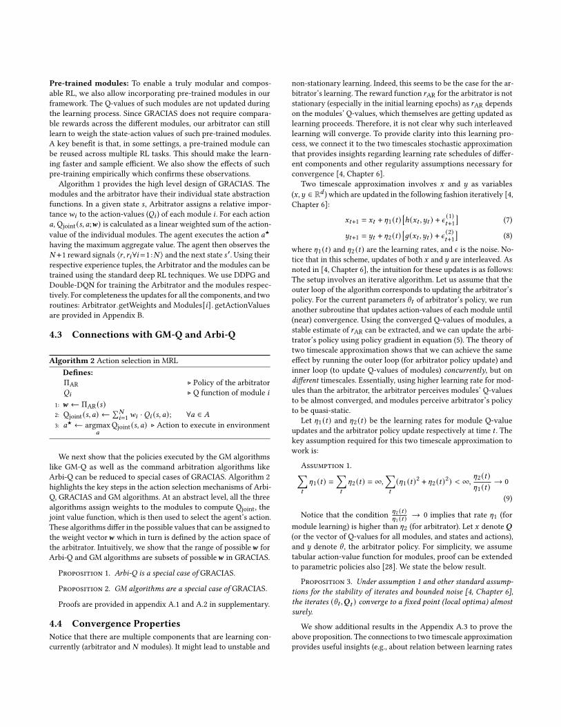
Pre-trained modules: To enable a truly modular and compos-
able RL, we also allow incorporating pre-trained modules in our
framework. The Q-values of such modules are not updated during
the learning process. Since GRACIAS does not require compara-
ble rewards across the different modules, our arbitrator can still
learn to weigh the state-action values of such pre-trained modules.
A key benefit is that, in some settings, a pre-trained module can
be reused across multiple RL tasks. This should make the learn-
ing faster and sample efficient. We also show the effects of such
pre-training empirically which confirms these observations.
Algorithm 1 provides the high level design of GRACIAS. The
modules and the arbitrator have their individual state abstraction
functions. In a given state 𝑠 , Arbitrator assigns a relative impor-
tance𝑤𝑖 to the action-values (𝑄𝑖 ) of each module 𝑖 . For each action
𝑎, Qjoint (𝑠, 𝑎;𝒘) is calculated as a linear weighted sum of the action-
value of the individual modules. The agent executes the action 𝑎★
having the maximum aggregate value. The agent then observes the
𝑁 +1 reward signals ⟨𝑟, 𝑟𝑖∀𝑖 =1 :𝑁 ⟩ and the next state 𝑠 ′. Using theirrespective experience tuples, the Arbitrator and the modules can be
trained using the standard deep RL techniques. We use DDPG and
Double-DQN for training the Arbitrator and the modules respec-
tively. For completeness the updates for all the components, and two
routines: Arbitrator·getWeights and Modules[𝑖] . getActionValuesare provided in Appendix B.
4.3 Connections with GM-Q and Arbi-Q
Algorithm 2 Action selection in MRL
Defines:ΠAR ⊲ Policy of the arbitrator
𝑄𝑖 ⊲ Q function of module 𝑖
1: 𝒘 ← ΠAR (𝑠)2: Qjoint (𝑠, 𝑎) ←
∑𝑁𝑖=1𝑤𝑖 ·𝑄𝑖 (𝑠, 𝑎); ∀𝑎 ∈ 𝐴
3: 𝑎★← argmax
𝑎Qjoint (𝑠, 𝑎) ⊲ Action to execute in environment
We next show that the policies executed by the GM algorithms
like GM-Q as well as the command arbitration algorithms like
Arbi-Q can be reduced to special cases of GRACIAS. Algorithm 2
highlights the key steps in the action selection mechanisms of Arbi-
Q, GRACIAS and GM algorithms. At an abstract level, all the three
algorithms assign weights to the modules to compute Qjoint, the
joint value function, which is then used to select the agent’s action.
These algorithms differ in the possible values that can be assigned to
the weight vector𝒘 which in turn is defined by the action space of
the arbitrator. Intuitively, we show that the range of possible𝒘 for
Arbi-Q and GM algorithms are subsets of possible𝒘 in GRACIAS.
Proposition 1. Arbi-Q is a special case of GRACIAS.
Proposition 2. GM algorithms are a special case of GRACIAS.
Proofs are provided in appendix A.1 and A.2 in supplementary.
4.4 Convergence PropertiesNotice that there are multiple components that are learning con-
currently (arbitrator and 𝑁 modules). It might lead to unstable and
non-stationary learning. Indeed, this seems to be the case for the ar-
bitrator’s learning. The reward function 𝑟AR for the arbitrator is not
stationary (especially in the initial learning epochs) as 𝑟AR depends
on the modules’ Q-values, which themselves are getting updated as
learning proceeds. Therefore, it is not clear why such interleaved
learning will converge. To provide clarity into this learning pro-
cess, we connect it to the two timescales stochastic approximation
that provides insights regarding learning rate schedules of differ-
ent components and other regularity assumptions necessary for
convergence [4, Chapter 6].
Two timescale approximation involves 𝑥 and 𝑦 as variables
(𝑥,𝑦 ∈ R𝑑 ) which are updated in the following fashion iteratively [4,Chapter 6]:
𝑥𝑡+1 = 𝑥𝑡 + [1 (𝑡)[ℎ(𝑥𝑡 , 𝑦𝑡 ) + 𝜖 (1)𝑡+1
](7)
𝑦𝑡+1 = 𝑦𝑡 + [2 (𝑡)[𝑔(𝑥𝑡 , 𝑦𝑡 ) + 𝜖 (2)𝑡+1
](8)
where [1 (𝑡) and [2 (𝑡) are the learning rates, and 𝜖 is the noise. No-tice that in this scheme, updates of both 𝑥 and 𝑦 are interleaved. As
noted in [4, Chapter 6], the intuition for these updates is as follows:
The setup involves an iterative algorithm. Let us assume that the
outer loop of the algorithm corresponds to updating the arbitrator’s
policy. For the current parameters \𝑡 of arbitrator’s policy, we run
another subroutine that updates action-values of each module until
(near) convergence. Using the converged Q-values of modules, a
stable estimate of 𝑟AR can be extracted, and we can update the arbi-
trator’s policy using policy gradient in equation (5). The theory of
two timescale approximation shows that we can achieve the same
effect by running the outer loop (for arbitrator policy update) and
inner loop (to update Q-values of modules) concurrently, but ondifferent timescales. Essentially, using higher learning rate for mod-
ules than the arbitrator, the arbitrator perceives modules’ Q-values
to be almost converged, and modules perceive arbitrator’s policy
to be quasi-static.
Let [1 (𝑡) and [2 (𝑡) be the learning rates for module Q-value
updates and the arbitrator policy update respectively at time 𝑡 . The
key assumption required for this two timescale approximation to
work is:
Assumption 1.∑𝑡
[1 (𝑡) =∑𝑡
[2 (𝑡) = ∞,∑𝑡
([1 (𝑡)2 + [2 (𝑡)2) < ∞,[2 (𝑡)[1 (𝑡)
→ 0
(9)
Notice that the condition[2 (𝑡 )[1 (𝑡 ) → 0 implies that rate [1 (for
module learning) is higher than [2 (for arbitrator). Let 𝑥 denote 𝑸(or the vector of Q-values for all modules, and states and actions),
and 𝑦 denote \ , the arbitrator policy. For simplicity, we assume
tabular action-value function for modules, proof can be extended
to parametric policies also [28]. We state the below result.
Proposition 3. Under assumption 1 and other standard assump-tions for the stability of iterates and bounded noise [4, Chapter 6],the iterates (\𝑡 ,𝑸𝑡 ) converge to a fixed point (local optima) almostsurely.
We show additional results in the Appendix A.3 to prove the
above proposition. The connections to two timescale approximation
provides useful insights (e.g., about relation between learning rates
of different components), and shows convergence properties under
some assumptions. In practical implementation, there are additional
details which we did not include for clarity of exposition (e.g., there
is a critic which is also learned for the arbitrator, Q-values for
modules are approximated using function approximators). The
above two timescale approximation analysis can also be extended
to such multi-timescale approximation also [28].
5 EXPERIMENTSWe showcase the effectiveness of GRACIAS on two well known
MRL domains, namely "Bunny World" [24, 25] and "Racetrack"
[19]. Besides these, we also use a complex Atari domain Qbert and
propose it as a new MRL benchmark. We compare against popular
MRL methods GM-Q and Arbi-Q as baselines. We also use Double-
DQN (DDQN) algorithm [30] as the standard deep RL baseline.
5.1 Hyperparameters and setupAppendix G (in supplementary) describes all the three domains and
their respective subtasks in detail. The arbitrator in GRACIAS can
use any RL algorithm that can optimize continuous actions. For our
experiments, the arbitrator is trained using DDPG algorithm [14].
The modules for all the approaches (GM-Q, Arbi-Q, and GRACIAS)
use the Double-DQN [30] algorithm to learn their subtasks. All the
hyperparameters and components such as network architecture,
state abstraction functions and experience replay memory for the
modules were kept the same across all the algorithms. For Qbert,
the modules use the same network architecture as proposed in [16].
The network architecture used in the Racetrack and Bunny World
is explained in the Appendix E (supplementary).
All the agents are trained using standard exploration techniques.
The DDQN baseline uses the epsilon-greedy exploration policy [32].
Similarly, GM-Q computesQjoint and uses the epsilon greedy policy
to select the action. InGRACIAS, the arbitrator outputs themodules’
weights, and adds a uniform random noise to these weights with
epsilon probability. The Qjoint is calculated using these weights,
and the action with the highest aggregate is executed.
We perform a set of four experiments (sections 5.2-5.5), each
highlighting a specific aspect of our algorithm. Five different in-
stances of each algorithm were trained using different random
seeds. The x-axis represents the training epochs, while the y-axis
represents the average episode reward over 15 trials based on the
fixed policy at that point (averaged over 5 random seeds). The solid
curves correspond to the mean, and the shaded regions capture
the minimum and maximum returns over five trials (plots with
min/max returns are shown in Appendix F). A running average of
15 was used in plotting the results.
5.2 Incomparable Reward Scales SettingFigure 3 shows the performance comparison among different algo-
rithms when the modules have incomparable or misaligned reward
scales. As defined in Appendix C, incomparable rewards imply that
rewards for individual modules are internally consistent, but are
incomparable to other modules’ reward scales. Designing compa-
rable rewards across all the modules is burdensome for domain
experts [24] and becomes even harder with a large number of
modules. We generated several candidate reward settings (shown
in tables 1, 2, 3 in supplementary). Only the GM-Q algorithm is
known to be highly sensitive to modules’ reward scales; GRACIAS
and Arbi-Q are robust to different reward scales (also shown in
section 5.5). Therefore, we selected a reward setting (indexed #5 in
table 1 and indexed #2 in table 2 and 3 in supplementary) for which
GM-Q did not perform well.
We observe that GM-Q cannot adapt to the misaligned reward
scale and converges to a suboptimal solution. Although both Arbi-
Q and GRACIAS are robust to reward scales, Arbi-Q has a slower
learning curve and converges to a suboptimal solution. In contrast,
GRACIAS can learn a good policy and converge faster than other
approaches. The graphs also show that even with a slow learning
curve DDQN baseline can eventually converge to a similar solution
as GRACIAS. We present below some insights for these results.
GM algorithms are unable to learn the importance of different
modules and assign equal weight to them. With misaligned re-
ward scales, some modules might overpower the contribution of
other modules in deciding the joint policy. For instance, in the
Bunny World domain, if the rewards of the 𝐶𝑜𝑙𝑙𝑒𝑐𝑡𝐹𝑜𝑜𝑑 module
are much larger compared to those of the 𝐴𝑣𝑜𝑖𝑑𝑃𝑟𝑒𝑑𝑎𝑡𝑜𝑟 module
(which is the case for the chosen reward setting), then the agent
will tend to ignore the action-values (and hence the preferences)
of the 𝐴𝑣𝑜𝑖𝑑𝑃𝑟𝑒𝑑𝑎𝑡𝑜𝑟 module. Therefore, the overall policy will be
unable to dodge the predator, and the agent will die quickly. As
shown in the graphs, such behavior causes the agent to converge
to a suboptimal policy.
As discussed earlier, Arbi-Q transfers the agent’s complete con-
trol to a single module and fails to find actions reasonable to all
modules. For instance, in the Bunny World domain, the predator
follows the agent almost always; hence the agent can not ignore
it in any state. If the control is given to the food module in any
state, the agent will completely ignore the predator, which can
lead to its death. On the other hand, if the control always remains
with the predator module, the agent ignores collecting food. This
behavior can be observed in the graphs where Arbi-Q converges
to suboptimal policies. It also has a much slower learning curve
compared to other algorithms. Similar trends can also be observed
in the experiments conducted in figures 2 & 3 of [24]. Note that
the figures for GM-SARSA and Arbi-Q have different scales on the
x-axis. Arbi-Q is slower than GM-SARSA by orders of magnitude,
the reasons for which were not discussed in that paper.
GRACIAS explores different weights for the modules and learns
to find a weight𝒘 that results in a good action selection that also
optimizes the global reward. By assigning appropriate importance
to different modules,GRACIAS can handle cases where the rewards
of some of the modules are very high and prevent them from dom-
inating the joint policy. Results in figure 3 for different domains
validate this observation. Experiments show that our approach
adapts well even to misaligned reward scales and converges to a
good quality policy.
In DDQN, a monolithic agent deals with the joint state space
containing complete information about all the subtasks. State space
grows exponentially in the number of state features due to the
curse of dimensionality, resulting in slower learning. However, the
availability of all this information also enables DDQN to converge to
a good policy eventually. On the other hand, in MRL, each module
solves a problem with a smaller state space resulting in better
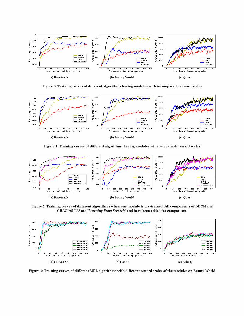
(a) Racetrack (b) Bunny World (c) Qbert
Figure 3: Training curves of different algorithms having modules with incomparable reward scales
(a) Racetrack (b) Bunny World (c) Qbert
Figure 4: Training curves of different algorithms having modules with comparable reward scales
(a) Racetrack (b) Bunny World (c) Qbert
Figure 5: Training curves of different algorithms when one module is pre-trained. All components of DDQN andGRACIAS-LFS are "Learning From Scratch" and have been added for comparison.
(a) GRACIAS (b) GM-Q (c) Arbi-Q
Figure 6: Training curves of different MRL algorithms with different reward scales of the modules on Bunny World

learning curves. Even for Qbert, where each module’s state space is
the same as DDQN, GRACIAS has better convergence than DDQN
as each module receives its subtask specific reward signal, which
results in better credit assignment and faster learning.
5.3 Comparable Reward Scale SettingFigure 4 shows the performance comparison of different algorithms
when all the modules have comparable reward scales. As discussed
above, only GM-Q is sensitive to the reward scales of the modules.
In Appendix C (supplementary), we do a grid search over the reward
scales of different modules (tables 1-3). We call a reward setting
comparable usingwhichGM-Q can achieve a solutionwhose quality
is similar to that achieved by DDQN on convergence. This set of
comparable rewards was then used for all the algorithms.
As evident from the graphs, both GRACIAS and GM-Q have bet-
ter learning curves and a faster rate of convergence as compared to
DDQN. Arbi-Q has a slow learning curve and converges to subopti-
mal policies. We can also see that despite the slower learning curve,
DDQN baseline is able to achieve good performance eventually. All
these observations are in line with the previous set of experiments.
A key observation is that even after prolonged training, GM-Q is
unable to learn a good policy in Qbert. We believe that this happens
because the GM algorithms fail to assign state-specific importance
to modules. Different modules fulfill different subtasks, and there-
fore, their importance across states might vary. Hence, assigning a
fixed importance to a module across all the states might hamper
the agent’s performance. However, in some domains like the Bunny
World, this phenomenon might not cause any significant perfor-
mance degradation. In the Bunny World, the agent has to dodge
the predator and consume all the food particles. It can not afford to
ignore the predator since that might cause its death. Moreover, the
predator module is indifferent between all the actions which do not
lead to its immediate death. An optimal policy would choose from
only these actions. This can be achieved by giving importance to
the𝐶𝑜𝑙𝑙𝑒𝑐𝑡𝐹𝑜𝑜𝑑 module that is just enough to break the tie between
these actions. Any static scaling that assigns adequate importance
to the 𝐴𝑣𝑜𝑖𝑑𝑃𝑟𝑒𝑑𝑎𝑡𝑜𝑟 module satisfies this requirement. Therefore
a single scaling might work equally well in Bunny World.
We also notice that GRACIAS is slightly slower than GM-Q in
the initial phases. It is because the GRACIAS’ arbitrator has to
learn the weights of different modules from scratch. It does so by
exploring different weight assignments𝒘 before converging to a
good policy. GM-Q on the other hand simply adds up the action
values of the modules and does not require any learning.
5.4 Learning with Pre-trained ModulesThe modules of a given complex task can be authored by different
dedicated experts. To realise the complete potential of MRL, the
knowledge from these modules should be composable, and the
components usable without any modification. In many cases, a
module might have been trained for a particular use case and made
available to the agent in a completely different context. An ideal
arbitrator would directly incorporate such modules and result in
sample efficient training. Therefore, we test the setting wherein
some of the modules are pre-trained and made available to the
arbitrator beforehand.
Figure 5 shows performance comparisons of different algorithms.
Conventional RL techniques for solving the monolithic RL tasks fail
to leverage pre-trainedmodules. The plots for DDQN andGRACIAS
("Learning From Scratch" in the normal setting) have been added
for comparisons. As in previous experiments, Arbi-Q converges
to suboptimal policies, and GM-Q suffers from the reward scale
incomparability and converges to suboptimal solutions. This exper-
iment highlights that GRACIAS can synchronize different modules
even when they are at different stages of their individual learning,
and fully leverages pre-trained modules for faster convergence.
We observe similar performance boost in GRACIAS when all the
modules are pre-trained and provided to the agent beforehand, and
only the arbitrator’s policy is learned (Appendix D, supplementary).
Even in this setting, GRACIAS learns a good policy.
5.5 Sensitivity to Modules’ Reward ScalesFigure 6 shows the training curves of each MRL algorithm when
trained across a spectrum of five different reward scales of the
modules on Bunny World. The graphs for Racetrack and Qbert, the
reward settings used for this experiment and the process of selecting
those rewards is described in Appendix C in supplementary.
We observe that GM-Q is unstable and converges to a lower
score on many reward scales. Arbi-Q, although indifferent to the
reward scales, consistently has slower learning curves and con-
verges to suboptimal policies. In contrast, GRACIAS is robust and
adapts well to even highly skewed reward scales. This robustness of
GRACIAS is the chief enabler of the truly modular RL framework
allowing modules to be transferred across different systems without
re-engineering their reward signals.
6 CONCLUSIONThis work is a first step towards making MRL scalable and com-
patible with modern deep RL approaches. We developed a novel
framework called GRACIAS for modular RL to solve complex real
world problems by decomposing it into simpler subtasks. GRACIAS
allows concurrent learning for such subtasks via separate modules,
which may have different subgoals. It can also leverage the knowl-
edge of pre-trained modules. A key enabler of such composable and
modular learning is our novel technique to train the arbitrator us-
ing deep RL algorithms by considering both the global reward and
the modules’ action preferences. Empirically, we demonstrate the
efficacy of GRACIAS on a range of problems against several MRL
algorithms. GRACIAS is able to overcome all the major limitations
of the existing MRL approaches and was observed to be highly
robust even when the rewards of the modules were incompara-
ble. Thus, our framework provides significant benefits for practical
applications of MRL for large scale learning problems.
ACKNOWLEDGMENTSWe thank Kohli Center on Intelligent Systems, International In-
stitute of Information Technology, Hyderabad for the generous
support. This research is also supported by the Ministry of Educa-
tion, Singapore under its MOE Academic Research Funding Tier 2
(Award MOE2018-T2-1-179). Any opinions, findings, and conclu-
sions are those of the author(s) and do not reflect the views of the
Ministry of Education, Singapore.

REFERENCES[1] Adrian K. Agogino and Kagan Turner. 2004. Unifying temporal and structural
credit assignment problems. In International Joint Conference on AutonomousAgents and Multiagent Systems, Vol. 2. 980–987.
[2] Pierre Luc Bacon, Jean Harb, and Doina Precup. 2017. The option-critic architec-
ture. In AAAI Conference on Artificial Intelligence. 1726–1734.[3] Marc G Bellemare, Yavar Naddaf, Joel Veness, and Michael Bowling. 2013. The
arcade learning environment: An evaluation platform for general agents. Journalof Artificial Intelligence Research 47 (2013), 253–279.
[4] Vivek Borkar. 2008. Stochastic Approximation: A Dynamical Systems Viewpoint.[5] Hyunjin Chang and Taeseok Jin. 2013. Command fusion based fuzzy controller
design for moving obstacle avoidance of mobile robot. In Future informationcommunication technology and applications. Springer, 905–913.
[6] Ivana Dusparic and Vinny Cahill. 2009. Distributed w-learning: Multi-policy op-
timization in self-organizing systems. In 2009 Third IEEE international conferenceon self-adaptive and self-organizing systems. IEEE, 20–29.
[7] Carlos Florensa, David Held, Markus Wulfmeier, Michael Zhang, and Pieter
Abbeel. 2017. Reverse curriculum generation for reinforcement learning. arXivpreprint arXiv:1707.05300 (2017).
[8] Tuomas Haarnoja, Aurick Zhou, Pieter Abbeel, and Sergey Levine. 2018. Soft
actor-critic: Off-policy maximum entropy deep reinforcement learning with a
stochastic actor. In International Conference on Machine Learning. 2976–2989.[9] Mark Humphrys. 1995. W-learning: Competition among selfish Q-learners. Tech-
nical Report. University of Cambridge.
[10] Mark Humphrys. 1996. Action selection methods using reinforcement learning.
From Animals to Animats 4 (1996), 135–144.[11] Yoram Koren, Johann Borenstein, et al. 1991. Potential field methods and their
inherent limitations for mobile robot navigation.. In ICRA, Vol. 2. 1398–1404.[12] Nevena Lazic, Tyler Lu, Craig Boutilier, Moonkyung Ryu, Eehern Wong, Binz
Roy, and Greg Imwalle. 2018. Data center cooling using model-predictive control.
In Advances in Neural Information Processing Systems. 3814–3823.[13] Sergey Levine, Chelsea Finn, Trevor Darrell, and Pieter Abbeel. 2016. End-to-end
training of deep visuomotor policies. The Journal of Machine Learning Research17, 1 (2016), 1334–1373.
[14] Timothy P Lillicrap, Jonathan J Hunt, Alexander Pritzel, Nicolas Heess, Tom Erez,
Yuval Tassa, David Silver, and Daan Wierstra. 2015. Continuous control with
deep reinforcement learning. arXiv preprint arXiv:1509.02971 (2015).[15] Timothy P. Lillicrap, Jonathan J. Hunt, Alexander Pritzel, Nicolas Heess, Tom Erez,
Yuval Tassa, David Silver, and DaanWierstra. 2016. Continuous control with deep
reinforcement learning. In International Conference on Learning Representations.[16] Volodymyr Mnih, Koray Kavukcuoglu, David Silver, Andrei A Rusu, Joel Veness,
Marc G Bellemare, Alex Graves, Martin Riedmiller, Andreas K Fidjeland, Georg
Ostrovski, et al. 2015. Human-level control through deep reinforcement learning.
nature 518, 7540 (2015), 529–533.[17] Andrew Y. Ng, Daishi Harada, and Stuart Russell. 1999. Policy invariance under
reward transformations : Theory and application to reward shaping. In Interna-tional Conference on Machine Learning. 278–287.
[18] Martin Riedmiller, Roland Hafner, Thomas Lampe, Michael Neunert, Jonas De-
grave, Tom Van de Wiele, Volodymyr Mnih, Nicolas Heess, and Jost Tobias Sprin-
genberg. 2018. Learning by playing-solving sparse reward tasks from scratch.
arXiv preprint arXiv:1802.10567 (2018).
[19] Stuart J Russell and Andrew Zimdars. 2003. Q-decomposition for reinforcement
learning agents. In Proceedings of the 20th International Conference on MachineLearning (ICML-03). 656–663.
[20] Alessandro Saffiotti, Kurt Konolige, and Enrique H Ruspini. 1995. A multivalued
logic approach to integrating planning and control. Artificial intelligence 76, 1-2(1995), 481–526.
[21] Gregor Schöner and Michael Dose. 1992. A dynamical systems approach to task-
level system integration used to plan and control autonomous vehicle motion.
Robotics and Autonomous systems 10, 4 (1992), 253–267.[22] D Silver, J Schrittwieser, K Simonyan, I Antonoglou Nature, and Undefined 2017.
2016. Mastering the game of Go without human knowledge. Nature 550, 7676(2016), 354.
[23] Christopher Simpkins, Sooraj Bhat, Charles Isbell, and Michael Mateas. 2008.
Towards adaptive programming integrating reinforcement learning into a pro-
gramming language. In International Conference on Object-Oriented ProgrammingSystems, Languages, and Applications. 603–613.
[24] Christopher Simpkins and Charles Isbell. 2019. Composable modular reinforce-
ment learning. In Proceedings of the AAAI Conference on Artificial Intelligence,Vol. 33. 4975–4982.
[25] Nathan Sprague and Dana Ballard. 2003. Multiple-goal reinforcement learning
with modular sarsa (0). (2003).
[26] Richard S Sutton and Andrew G Barto. 2018. Reinforcement learning: An intro-duction. MIT press.
[27] Richard S. Sutton, Doina Precup, and Satinder Singh. 1999. Between MDPs and
semi-MDPs: A framework for temporal abstraction in reinforcement learning.
Artificial Intelligence 112, 1 (1999), 181–211.[28] Chen Tessler, Daniel J. Mankowitz, and Shie Mannor. 2019. Reward constrained
policy optimization. In International Conference on Learning Representations, ICLR2019.
[29] John N Tsitsiklis. 1994. Asynchronous Stochastic Approximation and Q-Learning.
Machine Learning 16, 3 (1994), 185–202.
[30] Hado Van Hasselt, Arthur Guez, and David Silver. 2015. Deep reinforcement
learning with double q-learning. arXiv preprint arXiv:1509.06461 (2015).[31] Mnih Volodymyr, Kavukcuoglu Koray, Silver David, Rusu Andrei A, Veness
Joel, Bellemare Marc G, Graves Alex, Riedmiller Martin, Fidjeland Andreas K,
and Ostrovski Georg. 2015. Human-level control through deep reinforcement
learning. Nature 518, 7540 (2015), 529.[32] Christopher John Cornish HellabyWatkins. 1989. Learning from delayed rewards.
(1989).
[33] Shangtong Zhang. 2018. Modularized Implementation of Deep RL Algorithms in
PyTorch. https://github.com/ShangtongZhang/DeepRL.