modular robot design synthesis with deep reinforcement
TRANSCRIPT

Modular Robot Design Synthesis with Deep Reinforcement Learning
Julian Whitman1, Raunaq Bhirangi2, Matthew Travers2, Howie Choset2
1Department of Mechanical Engineering, Carnegie Mellon University2The Robotics Institute, Carnegie Mellon University5000 Forbes Ave., Pittsburgh, Pennsylvania 15213
Abstract
Modular robots hold the promise of versatility in that theircomponents can be re-arranged to adapt the robot design toa task at deployment time. Even for the simplest designs, de-termining the optimal design is exponentially complex dueto the number of permutations of ways the modules can beconnected. Further, when selecting the design for a giventask, there is an additional computational burden in evaluat-ing the capability of each robot, e.g., whether it can reachcertain points in the workspace. This work uses deep rein-forcement learning to create a search heuristic that allows usto efficiently search the space of modular serial manipulatordesigns. We show that our algorithm is more computation-ally efficient in determining robot designs for given tasks incomparison to the current state-of-the-art.
1 IntroductionModular robots offer the potential to create customizedrobots that can be readily deployed to perform a varietyof tasks. Synthesizing the design of a modular robot fora given task involves a number of challenges, one beingthat the space of possible module arrangements (ordered se-quences of discrete robotic modules) grows exponentially inthe number of types of modules and ways they can be con-nected. When searching this exponentially large space, wehave to evaluate whether each candidate robot can completethe task. This evaluation requires planning for and compar-ing the relative costs of motions for each candidate, whichis computationally intractable at scale. We address this in-tractability by learning a search heuristic which implicitlyencodes robot performance under the evaluation metric. Themain contribution of this work is an algorithm which usesdeep reinforcement learning to create this heuristic, enablingus to efficiently search the space of arrangements in the con-text of each robot’s inherent capabilities for a given task. Welimit the scope of the problem to synthesizing the arrange-ments of modular serial manipulators, for tasks in which themanipulator must reach a set of quasi-static workspace po-sitions and orientations.
We build on prior modular design synthesis methods (De-sai, Yuan, and Coros 2017; Ha et al. 2018) which incre-mentally construct and search a tree of different modular
PREPRINT: To appear in the proceedings of the 2020 AAAI Con-ference on Artificial Intelligence.
Figure 1: Our approach searches for modular manipulatordesigns by viewing the space of arrangements as a tree,where modules are sequentially added to the end of therobot. The arrangement at the root of the tree is a basemounting location. Solid arrows represent module additions,and dashed arrows indicate that the tree continues but is notshown. We use deep reinforcement learning to create a data-driven search heuristic which guides search on this tree. Weapply our algorithm to modular components produced byHebi Robotics (Hebi Robotics 2019).
arrangements. Specifically, each node added as a child toa current leaf node represents adding a module to the distalend of the manipulator, as shown in Figure 1. We view theconstruction of this tree as a series of states (arrangements)and actions (adding modules), and treat assembly of an ar-rangement as a Markov Decision Process (Sutton 1988). Un-der this formulation, we learn a state-action value functionwhich approximates the benefit of adding each module typeto an arrangement given the task. We train a deep Q-network

(DQN) to approximate this value function using reinforce-ment learning (Mnih et al. 2015). The DQN is used withina search heuristic for a best-first graph search (Bhardwaj,Choudhury, and Scherer 2017). The heuristic estimates thepotential for a branch of the search tree to contain a low-costrobot which completes the task.
We compare our approach to two related methods whichsearch for modular arrangements: a best-first search (Ha etal. 2018) and an evolutionary search (Icer et al. 2017). Aftertraining the DQN, our algorithm finds lower-cost solutionsmore efficiently than these related methods.
The rest of this paper is organized as follows: Section2 discusses related work on robot design synthesis, workthat motivated our approach, and a brief review of deep Q-learning. Section 3 describes our methodology for trainingthe DQN and searching the space of modular arrangements.Section 4 presents our results and benchmarks them againstexisting approaches. Sections 5 and 6 discuss the limitationsof our approach, future work, and concluding remarks.
2 BackgroundOur approach draws inspiration both from recent discretemodular design search work and from literature on the useof deep reinforcement learning for design and search.
2.1 Related WorkThe most closely related methods for manipulator arrange-ment synthesis are best-first graph searches (Desai, Yuan,and Coros 2017; Desai et al. 2018; Ha et al. 2018). In theseworks, a heuristic was crafted that estimated the ability ofeach partially complete arrangement in fulfilling the task,and was used to guide a search over a tree of different ar-rangements. The evaluation of their heuristics involved solv-ing an optimization subproblem, which becomes computa-tionally burdensome as the number of possible module typesand connections grows. Further, the heuristics did not con-sider obstacles, self-collisions, or torque constraints.
Another arrangement search method is a pruned exhaus-tive search. Althoff et al. (2019) performed increasinglycomputationally expensive checks on arrangements, elimi-nating candidates based on criteria such as total length orstatic torques. This method requires the evaluation criteria bemanually specified for each task and module set, and couldbecome computationally expensive en masse given an expo-nentially large search space.
Evolutionary algorithms have been used for design syn-thesis (Chen 1996; Leger 2012; Icer et al. 2017), searchingthe design space by randomly varying arrangements whileselecting for those with high fitness. These methods allowthe evaluation of many candidates in parallel, and work withdiscrete spaces. But, any domain-specific knowledge mustbe encoded by the user, the results of these algorithms varysubstantially between runs, and they are computationally ex-pensive because many candidate robots must be evaluated.
Deep RL has recently been used for robot design (Schaffet al. 2018; Ha 2018) to simultaneously learn a design and acontrol policy. Deep RL requires only a sparse reward func-tion be formulated for each task. RL has also been used to
design a deep neural network for image recognition (Bakeret al. 2016). We similarly learn the value of each sequentialdiscrete choice. These works use RL as the optimizer for asingle task; that is, they fix the task and environment thenuse RL to search for a design. They suffer from the time ittakes to optimize each design, thereby limiting their true po-tential, especially when rapidly prototyping designs or whenthe task may change frequently.
Our work is also inspired by recent work on learning-based motion planning. Chen, Murali, and Gupta (2018)learned a single control policy to control multiple robot de-signs, by training with a variety of manipulator designs onreaching and inserting a peg into a hole. As in our work, theirpolicy was conditioned on both the workspace target andthe robot design. Bhardwaj, Choudhury, and Scherer (2017)learned a search heuristic for a best-first search, used as apath planner in a grid world; we also learn a best-first searchheuristic, but in the context of design rather than planning.
2.2 Deep Q-learning for Modular Robot DesignWe formulate the robot design problem as a finite MarkovDecision Process, in which we construct a robot by addingone module at a time. We define a complete arrangement asone that ends with an end-effector module, and a partial ar-rangement as one that does not. At each time step t, the agentselects an action at that adds a module to a partial robot. Thestate st contains the arrangement, so the next state dependsdeterministically on only the previous state and the mod-ule added. This results in a new robot, st+1, and a reward,rt, from the environment. In this context the set of all robotmodules defines the action space A, while the set of partialand complete robots defines the state space, S.
We define the return at time t, Rt =∑Tt′=t γ
t−t′rt′ , witha discount factor 0 ≤ γ ≤ 1. The state-action value functionQπ : S×A 7→ R is then defined as the expected return giventhe action at is taken in state st following policy π : S 7→ A.Our approach uses reinforcement learning to estimate theoptimal state-action value functionQ∗, which can be definedin terms of the Bellman equation,
Q∗(st, at) = maxπ
E[rt + γmax
a′∈AQ∗(st+1, a
′)
]. (1)
Tabular Q-learning (Watkins 1989), a temporal differencelearning method (Sutton 1988), can be used to compute anestimate of the state-action value (“Q-value”) correspond-ing to every possible state-action pair. This approach be-comes intractable for large state and action spaces, so DeepQ-networks (DQN) use a deep neural network as a func-tion approximator Q(s, a; θ) with network parameters θ toapproximate Q∗(s, a) (Mnih et al. 2015). We train this net-work with experience replay (Riedmiller 2005) and a targetnetwork (Van Hasselt, Guez, and Silver 2016).
Our method also uses additions to the originalDQN framework. Universal value function approximators(UVFA) are learned value functions conditioned on the taskgoal (Schaul et al. 2015). We use a UVFA to enable ourDQN to apply to a range of goals. Hindsight experience re-play (HER) is a data augmentation technique employed for

RL problems with sparse reward signals (Andrychowicz etal. 2017). In HER, episodes are replayed with a differentgoal than the one used during the original episode.
3 MethodsIn contrast to recent work (Ha 2018; Schaff et al. 2018) thatused RL to solve an optimization problem to build a robotfor each task, we use RL to learn a UVFA for a class oftasks (Schaul et al. 2015). Specifically we use a DQN asa UVFA to learn the expected state-action value of addingeach module type to an arrangement given the goal of reach-ing a workspace target. The modules are chosen from a setof Nm types with indices m ∈ 1, 2, ...Nm. Each modulecould include any number of actuators and links, and may beable only to connect to some subset of other module types.The modular design synthesis problem is then to select a se-quence of modules which form an arrangement A that cancomplete a given task.
In this work we limit the space of tasks to a set of NTworkspace targets which a serial manipulator should reach.A workspace target T = [p, n̂] consists of a position in spacep ∈ R3 and tip axis orientation n̂ ∈ R3, ||n̂|| = 1. This rep-resentation can include manipulation tasks including peg-in-hole-insertion, positioning a camera, or screw insertion.
Let NJ(A) represent the number of actuated joints in agiven arrangement A. The forward kinematics (FK) of Awith joint angles ϑ ∈ RNJ (A)
[pEE , n̂EE ] = FK(A, ϑ), (2)
outputs pEE , the end-effector tip position, and n̂EE , the tipaxis. To evaluate whether an arrangement can reach a target,we define the inverse kinematics (IK) of an arrangement asthe joint angles that minimize the difference between the FKand a target,
ϑ = IK(A, p, n̂)
= argminϑ||p− pEE ||+ (1− n̂ · n̂EE)
s.t. f(A, ϑ) ≤ 0
(3)
where f represents a set of constraints including self-collision avoidance, obstacle-collision avoidance, and jointlimits. We use the interpenetration distance between collid-ing rigid bodies as the collision constraint metric. We solveIK numerically using gradient descent with multiple randominitial seed restarts. In a slight abuse of notation, we will usepEE(A, p, n̂) and n̂EE(A, p, n̂) to denote the forward kine-matics output of the inverse kinematics solution for a giventarget. To evaluate whether an arrangement can reach a giventarget, we set tolerances εp and εn, and define a “reachabil-ity” function for the arrangement as
reach(A, T ) =
1 ||p− pEE(A, p, n̂)|| ≤ εp and
1− n̂ · n̂EE(A, p, n̂) ≤ εn0 otherwise.
(4)
Our goal is to find an arrangement of modules that iscapable of reaching the targets. At the same time, we de-sire robots with fewer actuators (lower complexity) and
lower mass. However, we must recognize that for arbitraryenvironments and module type sets, not every target maybe reachable. Therefore, we pose this problem as a multi-objective optimization to maximize the number of targetsreached while minimizing the complexity and mass of therobot, which gives us an objective function F ,
F (A, T ) = −wJNJ(A)− wMM(A) + reach(A, T ) (5)
where we use M(A) to represent the total mass in arrange-ment A, and wJ and wM are user-set weighting factor totrade off between the multiple objectives. We seek an ar-rangement that maximizes this function,
A∗ = argmaxA
NT∑i=1
F (A, Ti). (6)
Next we will learn a neural network which approximates thebenefit of adding each module to an arrangement to maxi-mize (5) for a single target. Section 3.3 will describe howthis function is used to maximize over multiple targets.
3.1 DQN for module selectionOur algorithm assembles a serial-chain manipulator onemodule at a time, as illustrated in Figure 2. We use the out-put of a trained DQN to form a search heuristic. To use RL,we must first define the state, actions, and reward signals.
We encode the arrangement A as a list of one-hot vectors,where each index in a single vector indicates a type of mod-ule selected, with a user-set maximum number of modulesallowed in the arrangement Nmax. At each time step an ac-tion selects a module type m from the set of Nm moduletypes. Each episode is a series of steps where one moduleis added until either the arrangement is complete (an end-effector is added) or the maximum number of modules in anarrangement has been reached.
We append a single workspace target T = [p, n̂] tothe state. This conditions the Q-values on the target, form-ing a UVFA that can apply to a range of targets (Schaulet al. 2015). We also condition the learned Q-value func-tion on the locations of obstacles in the environment. Tomake a tractable parameterization of environment obsta-cles, we voxelize the space into a coarse “grid” and as-sign a binary occupied/unoccupied value to each voxel, soO ∈ {0, 1}(nO×nO×nO), where nO is the number of vox-els on each edge of the grid. The size of the voxels and therange of space over which they span were set by hand; weused nO = 5 with voxel edge length 0.25 m; see Figure 3for an illustration. The inputs to the DQN are the partial ar-rangement, the target, and the obstacle grid. Figure 4 depictsthe structure of the neural network.
We use a reward signal such that the sum of rewards overan episode matches (5) because we aim to select an arrange-ment that maximizes that function in (6). The non-terminalrewards are penalties assigned for the mass and complexityof each module m added to the arrangement,
r(m) = −wjNJ(m)− wMM(m). (7)
If the module added is an end-effector (EE), this is consid-ered a terminal action, and the terminal reward is returned.

Target
Obstacles
Addjoint
Addlink
Obstacles
(empty)DQN
Partial robot Partial robot Complete
robot
Evaluate robotand targetPartial robot DQN DQN
Base
(Multiple steps)
Figure 2: During training, the DQN is used repeatedly to evaluate the contribution each module type would have toward reachinga target. The arrangement is assembled sequentially (top) with modules selections made by the DQN (bottom)
The reachability function (4) is evaluated and added to thereward. If the maximum number of modules is reached with-out any end-effector added, a penalty of −1 is returned,
rterminal =
−1 length(A′) == Nmax
and m is not an EEreach(A′, T ) m is an EE,
(8)
where we define A′ as the arrangement resulting from theaddition of m to the existing arrangement A. The elementsof the Q-value vector Q ∈ R output by a forward pass of theDQN represent the expected value of a module type m thatcould be added to the tip of the arrangementA given a targetT and grid O,
Q(A, T,O,m) = E[r +max
m′Q(A′, T,O,m′)
]≈ DQNm(A, T,O),
(9)
where DQNm is the mth component of the output of theDQN, as shown in Fig. 4.
3.2 Training the DQNThe DQN is trained to approximate the Q-values of eachmodule type for a given arrangement, target, and grid. Atthe start of each episode during training we randomize thetarget and grid. Each element of p and n̂ is selected from a[−1, 1] range, and n̂ is normalized. When we randomize thetarget and environment occupancy, we ensure that any pointsthat must be occupied by the robot (e.g. the base and target)are unoccupied.
During training we build up an arrangement by sequen-tially selecting modules. At each step in the episode, the net-work outputs Q-values for each module type. In our moduleset, each type of module can connect to only a subset of theother module types. We mask out invalid module connec-tion actions, and only learn Q-values for valid actions. Anepisode ends when an EE module is chosen or the maximumnumber of allowable modules has been added. The episodeshave a maximum length, enabling us to use a discount fac-tor γ = 1. We use a Boltzmann exploration strategy (Barto,Bradtke, and Singh 1995), as there are multiple similar mod-ule choices with similar values that should be explored, such
that we avoid exploiting a single robot arrangement for alltasks. We use curriculum learning (Bengio et al. 2009) onthe obstacle grid, mass penalty, and complexity penalty. Webegin training with no obstacles or penalties, and periodi-cally increase the maximum number of randomly selectedobstacles and the penalty value during the early stages oftraining.
To learn from the sparse reward signal, we use HER(Andrychowicz et al. 2017). Each time a complete arrange-ment is found which does not reach the target, the episode isreplayed with the point that was reached set as the target. Weintroduce additional data augmentation by randomly sam-pling joint angles and occupancy grid for the robot found,calculating FK, removing any samples that are in collision,and replaying the episode with the pose reached by eachsample’s FK set as the target. We found this results in higherquality solutions to our full graph search procedure by train-ing the network to better predict the potential value of lowermass/complexity arrangements. While training, we periodi-cally test the DQN on a small set of randomly generated testpoints. The performance of the graph search procedure onthese test sets is used as an evalution metric to decide whento end training.
3.3 Using the DQN as a search heuristicTo search for task-specific arrangements, we use the DQNmodule value approximator to guide a best-first search. Theforward pass of the DQN outputs the Q-value for each mod-ule type conditioned on a single target and grid. This Q-valueencodes the expected future value of the objective functionF defined in (5).
Different tasks may involve reaching different numbers oftargets; as per (6), we seek to maximize return over multipletargets. But, for a single neural network to operate on multi-ple points at once, the value function would need to be con-ditioned on all permutations of those points, and would beconstrained to a fixed maximum number of points. It wouldbe significantly more computationally expensive to train ifeach arrangement selection were to be conditioned on a setof targets than if it were conditioned on one target. To ad-dress this challenge, we create a search heuristic from theoutput of one forward pass for each target.

Figure 3: Top: An arrangement of modules (dark greyand red) with base located at the origin reaches a singleworkspace target position and tip axis (green point witharrow) without colliding with voxelized obstacles (greycubes). Bottom: The physical modular robot matches the ar-rangement and environment.
First we observe that at terminal actions, the state-actionvalue summed over all targets matches the desired maxi-mization in (6). That is, for actions that result in terminalstates (when the selected action m is an end-effector),
NT∑i=1
Q(A, Ti, O,m) =
NT∑i=1
F (A′, Ti). (10)
Even though this equation is not exact for non-terminal ac-tions, we find that the summation over Q-values is a goodsearch heuristic to maximize objective F . Therefore weform the search heuristic h ∈ R from a summation of for-ward passes of the DQN for each target,
h(A, T1...TNT, O,m) =
NT∑i=1
DQNm(A, Ti, O). (11)
This search heuristic prioritizes modules selected based on
𝐴 [𝑝, ො𝑛] 𝑂
𝑄1𝑄2⋮
𝑄𝑁𝑚
Figure 4: The neural network architecture we used for ourDQN consists of fully connected (FC) layers with recti-fied linear unit (ReLU) activation, and a 3D convolution(Conv3D) over the grid of obstacles. The inputs to the DQNare the current arrangement A, target T = [p, n̂], and ob-stacle grid O. The outputs are the state-action values Q foreach type of module.
Algorithm 1: Manipulator arrangement search, a best-first search guided by the output of a DQN.
Input: A set of NT targets and an occupancy grid OResult: Arrangement Aopenset = [Empty arrangement]while time < time limit do
Pop node with highest h value from openset;Expand the node;if node contains complete robot then
Evaluate IK at all targets;if all targets reached then
Store return for the arrangementend
elseForward pass of DQN and sum output for eachtarget as in (11);
Add each child A′ to the openset with value hend
endReturn arrangement with highest return (lowest cost)
their potential to reach the targets with fewer additionalmodules.
Our DQN-best-first search algorithm is outlined in Algo-rithm 1. At each iteration, the arrangement with the highestheuristic value is popped from the open set. If it is a com-plete robot, it is evaluated. Otherwise it is expanded, passedthrough the DQN to create new h values for its children, andthose children are added to the open set.
The Q-value is the expected return from the current ar-rangement onward. We penalize the addition of modules,so the DQN outputs from arrangements with more modulesare usually higher than the outputs from arrangements withfewer modules. As a result, the search tends to act more likea depth-first search than a breadth-first search. A neural net-work forward pass is computationally inexpensive, so com-putation of this heuristic scales linearly with the number oftargets, keeping computation for each node expansion low.

3.4 Comparisons to related workWe implemented two methods from prior work, a geneticand a best-first search, as bases of comparison. Here we de-scribe these implementations and the experiments we ran.
Genetic algorithm Each individual A in the populationwas represented with a gene g ∈ [0, 1)Nmax . To convert eachgene to an arrangement, each element was interpreted se-quentially as the next valid module to attach. For example, ifthere are two possible children module types for the moduleat j − 1, and element j of the gene is 0 ≤ gj < 0.5, then thefirst of the two types would be selected, but if 0.5 ≤ gj < 1then the second of the two types would be selected. Each in-dividual in the population was evaluated with a score com-bining their IK error, weighted complexity and mass, andwhether they are complete. The population was resampledwith elite selection, crossover, and mutation.
Best-first search algorithm We implemented the algo-rithm of Ha et al. (2018), in which the tree of possible de-signs is explored with a best-first search. At each step, partialrobots are evaluated with a heuristic function based on anIK-like subproblem. The candidate with the lowest heuristiccost is expanded, and any complete robots are evaluated forthe specified task. We removed velocity constraints from theIK and heuristic subproblem evaluations, which speeds upthese functions which are evaluated many times.
Comparison tests We conducted a comparison test be-tween the different methods: a genetic algorithm, best-firstsearch, and our DQN-best-first search. We used modularcomponents produced by Hebi Robotics (Hebi Robotics2019) with a set of 11 types of modules: three base mountorientations, one actuated joint, six different links/brackets,and one end-effector. We limit the maximum number ofmodules in an arrangement to Nmax = 16, a sufficientlength for complete robots with a maximum of seven ac-tuated joints given these modules. During training and alltests, we set the objective weights wJ = 0.025, wM = 0.1.In the comparison tests, we generated 50 sets of 10 randomtargets, each set with a randomized obstacle grid with up to10 obstacles. For each method, we measured:• the time until the first feasible arrangement (one which
reaches all targets) was found for each set,• the standard deviation of the time until the first feasible
robot was found was found for each set,• the penalty wJNJ(A) + wMM(A) from the complexity
and mass of the first feasible robot,• the number of complete arrangements evaluated before a
feasible robot was found,• the feasible arrangement with the lowest cost found after
five minutes, and• the number of target sets for which no feasible arrange-
ment was found after five minutes.When no feasible arrangement was found for a given methodand set within the time limit, that set was not included inthe averages or times for that method. We selected thesecriteria because we are interested in rapid prototyping and
field applications, where we may need to trade off betweenspeed and solution quality. As such both the first arrange-ment found (fastest solution) and the solution found after afixed amount of time are relevant. The IK evaluation of com-plete robots is the most computationally expensive step. Wetrained the DQN and conducted all tests on a desktop com-puter with Ubuntu 16.04, Intel i5 four-core processor at 3.5GHz, and an NVIDIA GTX 1050 graphics card. We trainedthe DQN for 450,000 episodes (about 33 hours) before usingit within our algorithm.
Searching with torque constraints In addition to theDQN network above, we trained a network for a more dif-ficult variant of the problem, with more module types and aconstraint on the actuator torque limits. We added five moremodule types (four links and one rotary actuator), for 16 to-tal module types. One actuator module type had lower massand lower maximum torque, and the other had higher massand higher maximum torque. When evaluating the reachabil-ity function, if any actuator torque limit was exceeded, thena terminal reward of 0 was returned. As a basis of compari-son, we modified the genetic algorithm to include a penaltyon arrangements that overload the actuator torques. We wereunable to compare this extension to the method of (Ha et al.2018) as their method does not consider torques. The test setused in this test was the same as those described above. Wetrained this DQN for 700,000 episodes (about 57 hours).
4 ResultsThe results of the comparison tests are shown in Table 1.We found that our method produces the best results in allcategories. For one of the tests, none of the three algorithmswere able to find a feasible robot within five minutes.
The genetic algorithm finds costly feasible arrangementsin few iterations by randomly sampling arrangements, andthen refines those results over further iterations to less costlyarrangements. Qualitatively we found it tends to do wellwhen there are many feasible robots for the task, for exam-ple when there are few targets and few obstacles, becausethe initial sampling may include costly arrangements thatcomplete the task. However, the genetic algorithm requiresmany complete robot planning evaluations. If the computa-tional cost of evaluating planning for complete robots wereto increase, we expect this method to correspondingly be-come more expensive.
The best-first search does not include obstacles in itssearch heuristic, so its performance tends to degrade in thepresence of many obstacles. It evaluates robots in order ofincreasing complexity, but must solve an nonlinear programto evaluate each node. Due to this computationally expensivesubproblem, this algorithm was not able to find solutions fora third of the test cases within the five minute time limit. Inthe cases where it did find a solution, it was not usually ableto improve upon that solution within the remaining time.
We observed that our method acts depth-first initially,evaluating a complete robot after only a few DQN for-ward passes. The reward structure during training guides thesearch toward less costly arrangements. In contrast to theheuristic of (Ha et al. 2018), our heuristic considers obstacle
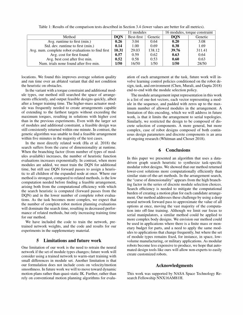
Table 1: Results of the comparison tests described in Section 3.4 (lower values are better for all metrics).11 modules 16 modules, torque constraint
Method DQN Best-first Genetic DQN GeneticAvg. runtime to first (min.) 0.26 3.04 0.64 0.20 3.08
Std. dev. runtime to first (min.) 0.14 1.00 0.69 0.38 1.69Avg. num. complete robot evaluations to find first 10.31 29.03 138.12 39.76 311.41
Avg. cost for first found 0.57 0.59 0.62 0.63 0.64Avg. best cost after five min. 0.52 0.58 0.53 0.60 0.63
Num. trials none found after five min. 1/50 16/50 1/50 1/50 28/50
locations. We found this improves average solution qualityand run time over an ablated variant that did not conditionthe heuristic on obstacles.
In the variant with a torque constraint and additional mod-ule types, our method still searched the space of arrange-ments efficiently, and output feasible designs quickly, albeitafter a longer training time. The higher-mass actuator mod-ule was frequently needed to create arrangements capableof extending to the farthest targets without exceeding themaximum torques, resulting in solutions with higher costthan in the previous experiments. Even with the larger setof modules and additional constraint, a feasible design wasstill consistently returned within one minute. In contrast, thegenetic algorithm was unable to find a feasible arrangementwithin five minutes in the majority of the test cases.
In the most directly related work (Ha et al. 2018) thesearch suffers from the curse of dimensionality at runtime.When the branching factor (from number of types of mod-ules available) increases, the number of heuristic functionevaluations increases exponentially. In contrast, when moremodules are added, we must train the DQN for additionaltime, but still use DQN forward passes to assign a heuris-tic to all children of the expanded node at once. Where ourmethod is strongest, compared to related methods, is the lowcomputation needed before finding a feasible arrangement,arising both from the computational efficiency with whichthe search heuristic is computed (forward passes from theDQN) and in the lower number of complete robot evalua-tions. As the task becomes more complex, we expect thatthe number of complete robot motion planning evaluationswill dominate the search time, resulting in decreased perfor-mance of related methods, but only increasing training timefor our method.
We have included the code to train the network, pre-trained network weights, and the code and results for ourexperiments in the supplementary material.
5 Limitations and future workOne limitation of our work is the need to retrain the neuralnetwork if the set of module types changes; future work willconsider using a trained network to warm-start training withsmall differences in module set. Another limitation is thatour formulation does not include costs on velocity/motionsmoothness. In future work we will to move toward dynamicmotion plans rather than quasi-static IK. Further, rather thanrely on conventional motion planning algorithms for evalu-
ation of each arrangement at the task, future work will in-volve learning control policies conditioned on the robot de-sign, task, and environment (Chen, Murali, and Gupta 2018)end-to-end with the module selection policy.
The module arrangement input representation in this workis a list of one-hot vectors, each vector representing a mod-ule in the sequence, and padded with zeros up to the max-imum number of allowed modules in the arrangement. Alimitation of this encoding, which we will address in futurework, is that it limits the arrangement to serial topologies.Similarly, we restricted the design to be composed of dis-crete selection of components. A more general, but morecomplex, case of robot designs composed of both contin-uous design parameters and discrete components is an areaof ongoing research (Whitman and Choset 2018).
6 Conclusions
In this paper we presented an algorithm that uses a data-driven graph search heuristic to synthesize task-specificmodular robot designs. We showed that our method returnedlower-cost solutions more computationally efficiently thansimilar state-of-the-art methods. In the arrangement search,the “curse of dimensionality” appears from the high branch-ing factor in the series of discrete module selection choices.Search efficiency is needed to mitigate the computationalburden of creating a motion plan for each candidate arrange-ment. Our method addresses these challenge by using a deepneural network forward pass to approximate the value of alloptions at once, moving the vast majority of the computa-tion into off-line training. Although we limit our focus toserial manipulators, a similar method could be applied tomore complex body designs. We envision our method couldbe used in applications where there is a finite mass or mon-etary budget for parts, and a need to apply the same mod-ules to applications that change frequently, but where the setof module types remains fixed, for instance, in space, low-volume manufacturing, or military applications. As modularrobots become less expensive to produce, we hope that auto-mated design tools like ours will allow non-experts to easilycreate customized robots.
Acknowledgments
This work was supported by NASA Space Technology Re-search Fellowship NNX16AM81H.
ReferencesAlthoff, M.; Giusti, A.; Liu, S.; and Pereira, A. 2019.Effortless creation of safe robots from modules throughself-programming and self-verification. Science Robotics4(31):eaaw1924.Andrychowicz, M.; Wolski, F.; Ray, A.; Schneider, J.; Fong,R.; Welinder, P.; McGrew, B.; Tobin, J.; Abbeel, O. P.; andZaremba, W. 2017. Hindsight experience replay. In Ad-vances in Neural Information Processing Systems, 5048–5058.Baker, B.; Gupta, O.; Naik, N.; and Raskar, R. 2016. Design-ing neural network architectures using reinforcement learn-ing. arXiv preprint arXiv:1611.02167.Barto, A. G.; Bradtke, S. J.; and Singh, S. P. 1995. Learn-ing to act using real-time dynamic programming. Artificialintelligence 72(1-2):81–138.Bengio, Y.; Louradour, J.; Collobert, R.; and Weston, J.2009. Curriculum learning. In Proceedings of the 26th an-nual international conference on machine learning, 41–48.ACM.Bhardwaj, M.; Choudhury, S.; and Scherer, S. 2017. Learn-ing heuristic search via imitation. In Conference on RobotLearning, 271–280.Chen, T.; Murali, A.; and Gupta, A. 2018. Hardware con-ditioned policies for multi-robot transfer learning. In Ad-vances in Neural Information Processing Systems, 9333–9344.Chen, I. M. 1996. On optimal configuration of modular re-configurable robots. In Proceedings of the 4th InternationalConference on Control, Automation, Robotics, and Vision.Desai, R.; Safonova, M.; Muelling, K.; and Coros, S. 2018.Automatic design of task-specific robotic arms. arXivpreprint arXiv:1806.07419.Desai, R.; Yuan, Y.; and Coros, S. 2017. Computational ab-stractions for interactive design of robotic devices. In 2017IEEE International Conference on Robotics and Automation(ICRA), 1196–1203. IEEE.Ha, S.; Coros, S.; Alspach, A.; Bern, J. M.; Kim, J.; andYamane, K. 2018. Computational design of robotic devicesfrom high-level motion specifications. IEEE Transactionson Robotics 34(5):1240–1251.Ha, D. 2018. Reinforcement learning for improving agentdesign. arXiv preprint arXiv:1810.03779.Hebi Robotics. 2019. [Online]. www.hebirobotics.com.Accessed Aug. 8, 2019.Icer, E.; Hassan, H. A.; El-Ayat, K.; and Althoff, M. 2017.Evolutionary cost-optimal composition synthesis of modularrobots considering a given task. In 2017 IEEE/RSJ Interna-tional Conference on Intelligent Robots and Systems (IROS),3562–3568. IEEE.Leger, C. 2012. Darwin2K: An evolutionary approach toautomated design for robotics, volume 574. Springer Sci-ence & Business Media.Mnih, V.; Kavukcuoglu, K.; Silver, D.; Rusu, A. A.; Ve-ness, J.; Bellemare, M. G.; Graves, A.; Riedmiller, M.;
Fidjeland, A. K.; Ostrovski, G.; et al. 2015. Human-level control through deep reinforcement learning. Nature518(7540):529.Riedmiller, M. 2005. Neural fitted q iteration–first expe-riences with a data efficient neural reinforcement learningmethod. In European Conference on Machine Learning,317–328. Springer.Schaff, C.; Yunis, D.; Chakrabarti, A.; and Walter, M. R.2018. Jointly learning to construct and control agentsusing deep reinforcement learning. arXiv preprintarXiv:1801.01432.Schaul, T.; Horgan, D.; Gregor, K.; and Silver, D. 2015.Universal value function approximators. In Proceedings ofthe 1st Annual Conference on Robot Learning, 1312–1320.Sutton, R. S. 1988. Learning to predict by the methods oftemporal differences. Machine learning 3(1):9–44.Van Hasselt, H.; Guez, A.; and Silver, D. 2016. Deep re-inforcement learning with double q-learning. In ThirtiethAAAI conference on artificial intelligence.Watkins, C. J. C. H. 1989. Learning from delayed rewards.Ph.D. Dissertation, King’s College, Cambridge.Whitman, J., and Choset, H. 2018. Task-specific manip-ulator design and trajectory synthesis. IEEE Robotics andAutomation Letters 4(2):301–308.