active filters - revisitedece347.cankaya.edu.tr/uploads/files/ece347_week8.pdf · active filters -...
TRANSCRIPT

Active Filters - Revisited
Sources:
Electronic Devices
by
Thomas L. Floyd.
&
Electronic Devices and Circuit Theory
by
Robert L. Boylestad, Louis Nashelsky

Ideal and Practical Filters
Ideal and Practical Filters

Ideal and Practical Filters
Quality Factor (Q) of a band-pass filter is the ratio of the
center frequency to the bandwidth.
The quality factor (Q) can also be expressed in terms of
the damping factor (DF) of the filter as

Ideal and Practical Filters
The Butterworth Characteristic
• Provides a very flat amplitude
response in the passband and a roll-
off rate of -20 dB/decade/pole
• Phase response is not linear
• A pulse will cause overshoots on the
output because each frequency
component of the pulse’s rising and
falling edges experiences a different
time delay
• Normally used when all frequencies in
the passband must have the same
gain.
• Often referred to as a maximally flat
response.
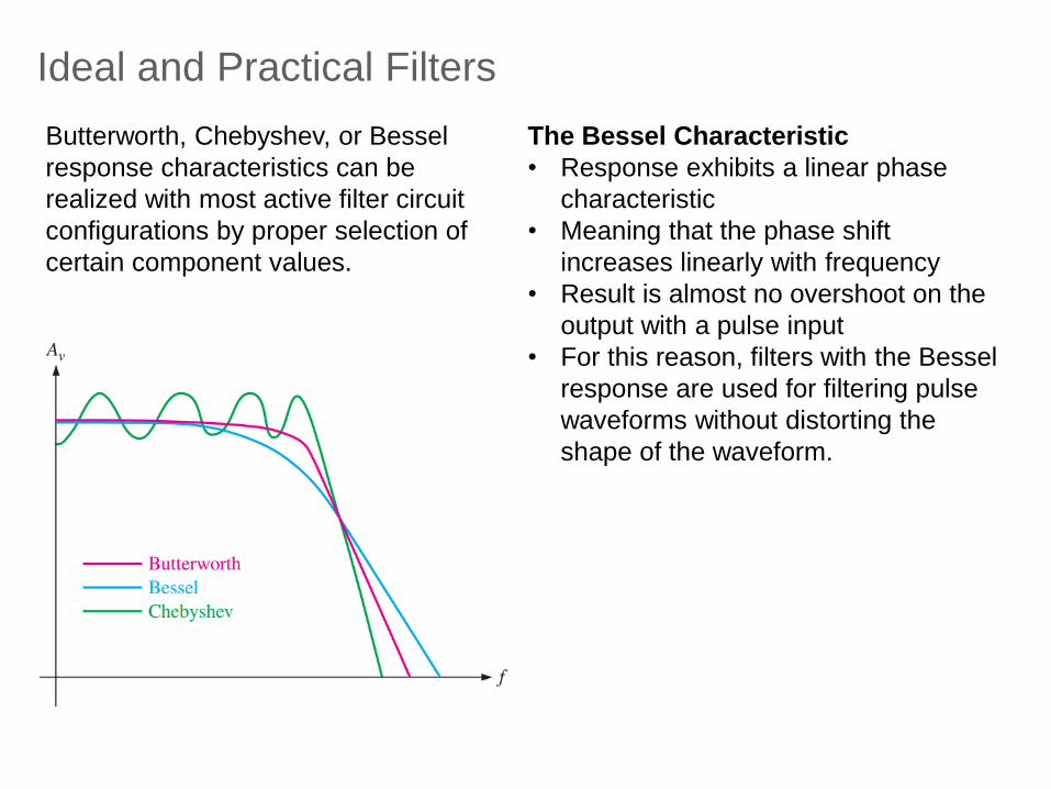
Butterworth, Chebyshev, or Bessel
response characteristics can be
realized with most active filter circuit
configurations by proper selection of
certain component values.

Ideal and Practical Filters
The Chebyshev Characteristic
• Useful when a rapid roll-off is required
• Because it provides a roll-off rate
greater than 20 dB/decade/pole
• Filters can be implemented with fewer
poles and less complex circuitry for a
given roll-off rate
• Characterized by overshoot or ripples
in the passband (depending on the
number of poles)
• and an even less linear phase
response than the Butterworth.
Butterworth, Chebyshev, or Bessel
response characteristics can be
realized with most active filter circuit
configurations by proper selection of
certain component values.
Ideal and Practical Filters
The Bessel Characteristic
• Response exhibits a linear phase
characteristic
• Meaning that the phase shift
increases linearly with frequency
• Result is almost no overshoot on the
output with a pulse input
• For this reason, filters with the Bessel
response are used for filtering pulse
waveforms without distorting the
shape of the waveform.
Butterworth, Chebyshev, or Bessel
response characteristics can be
realized with most active filter circuit
configurations by proper selection of
certain component values.

Ideal and Practical Filters
• An active filter can be designed to have
either a Butterworth, Chebyshev, or
Bessel response characteristic
regardless of whether it is a low-pass,
high-pass, band-pass,
• The damping factor (DF ) of an active
filter circuit determines which response
characteristic the filter exhibits
• A generalized active filter is shown
in figure below
• Includes an amplifier, a negative
feedback circuit, and a filter section
• Damping factor determined by
negative feedback circuit is given by

Ideal and Practical Filters
• Damping factor affects filter response by
negative feedback action
• Any attempted increase or decrease in the
output voltage is offset by the opposing effect
of the negative feedback
• This tends to make the response curve flat in
the passband of the filter if the value for the
damping factor is precisely set
• By advanced mathematics, which we will not
cover, values for the damping factor have
been derived for various orders of filters to
achieve the maximally flat response of the
Butterworth characteristic
• The value of the damping factor required to produce a desired response
characteristic depends on the order (number of poles) of the filter
• A pole, for our purposes, is simply a circuit with one resistor and one capacitor.
The more poles a filter has, the faster its roll-off rate is
• To achieve a second-order Butterworth response, for example, the damping
factor must be 1.414.

Ideal and Practical Filters
• To achieve a second-order Butterworth
response, for example, the damping factor
must be 1.414
• To implement this damping factor, the
feedback resistor ratio must be
• This ratio gives the closed-loop gain of the
noninverting amplifier portion of the filter,
derived as follows

Ideal and Practical Filters
• To produce a filter that has a steeper transition region it is necessary to add
additional circuitry to the basic filter.
• Responses that are steeper than in the transition region cannot be obtained
by simply cascading identical RC stages (due to loading effects)
• However, by combining an op-amp with frequency-selective feedback
circuits, filters can be designed with roll-off rates of or more dB/decade
• Filters that include one or more op-amps in the design are called active
filters
• These filters can optimize the roll-off rate or other attribute (such as phase
response) with a particular filter design
• In general, the more poles the filter uses, the steeper its transition region will
be
• The exact response depends on the type of filter and the number of poles

Ideal and Practical Filters
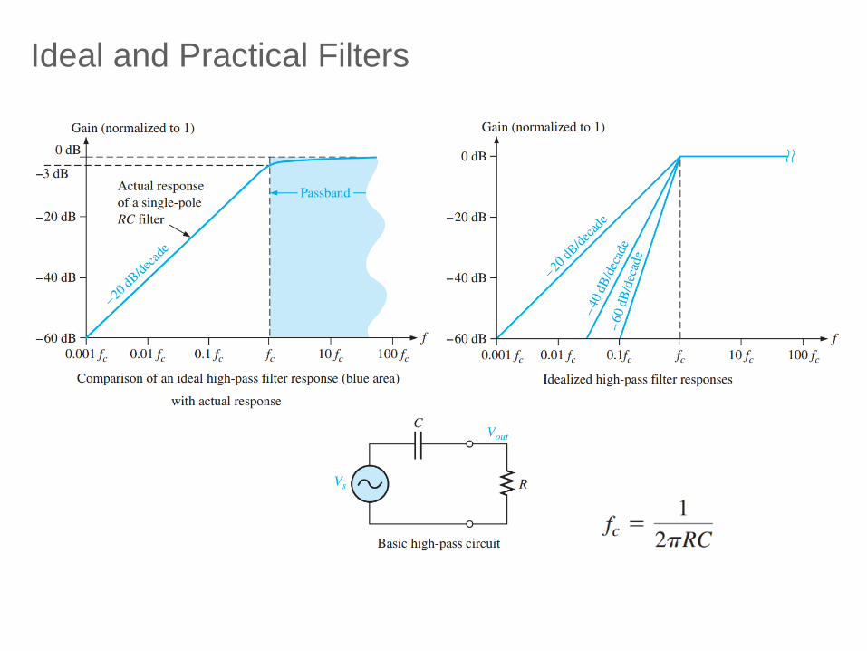
• The number of poles determines the roll-off rate of the filter
• A Butterworth response produces -20 dB/decade/pole
• a first-order (one-pole) filter has a roll-off of -20 dB/decade
• a second-order (two-pole) filter has a roll-off rate of -40 dB/decade
• a third-order (three-pole) filter has a roll-off rate of -60 dB/decade …
• Generally, to obtain a filter with three poles or more, one-pole or two-pole
filters are cascaded, as shown in figure below
• To obtain a third-order filter, for example, cascade a second-order and a
first-order filter
• To obtain a fourth-order filter, cascade two second-order filters; and so on ,
• Each filter in a cascaded arrangement is called a stage or section.

A Single Pole Low-Pass Filter
Active Filters – Low-Pass Filters

Active Filters – Low-Pass Filters

𝑉𝑜𝑉1
= 𝐴𝑣 = 1 +𝑅𝐹𝑅𝐺
1
1 + 𝑗𝜔𝑅1𝐶1
Real
number
(gain)
Low-pass
filter
𝑓𝑂𝐿 =1
2 𝜋𝑅1𝐶1
>1 for a
low-pass
filter
with
voltage
gain
cut-off
frequency
Active Filters – Low-Pass Filters

𝑉𝑜𝑉1
= 𝐴𝑣 = 1 +𝑅𝐹𝑅𝐺
1
1 + 𝑗𝜔𝑅1𝐶1
Real
number
(gain)
Low-pass
filter
𝑓𝑂𝐿 =1
2 𝜋𝑅1𝐶1
>1 for a
low-pass
filter
with
voltage
gain
cut-off
frequency
Active Filters – Low-Pass Filters

Active Filters – Low-Pass Filters

The Sallen-Key Low-Pass Filter • There are two low-pass RC circuits
that provide a roll-off of -40
dB/decade above the critical
frequency (assuming a Butterworth
characteristic)
• One RC circuit consists of RA and CA
and the second circuit consists of RB
and CB
• A unique feature is the capacitor that
provides feedback for shaping the
response near the edge of passband
• If RA = RB = R and CA = CB = C
Active Filters – Low-Pass Filters
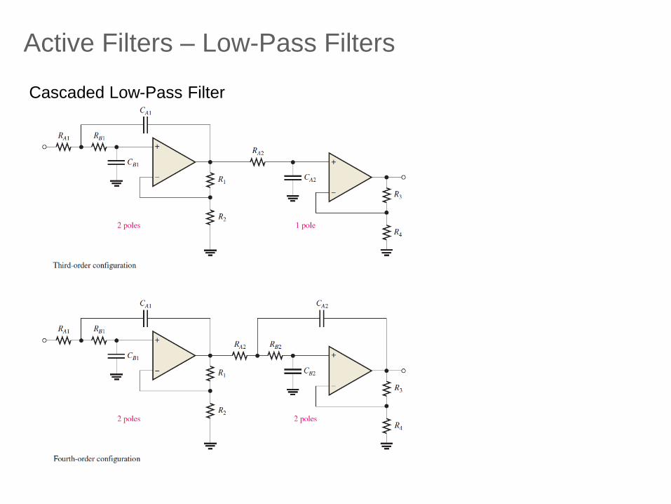
Cascaded Low-Pass Filter
Active Filters – Low-Pass Filters

Ideal and Practical FiltersValues for the Butterworth response
• Determine the
capacitance values for a
critical frequency of 2680
Hz if all the resistors in
the RC low-pass circuits
are 1.8 KΩ.
• Also select values for the
feedback resistors to get
a Butterworth response

Ideal and Practical Filters
• Determine the
capacitance values for a
critical frequency of
2680 Hz if all the
resistors in the RC low-
pass circuits are 1.8 KΩ.
• Also select values for
the feedback resistors to
get a Butterworth
response

Active Filters – High-Pass Filters
RC High-pass filter
𝐴𝑣 = 1 +𝑅𝐹𝑅𝐺
𝑓𝑂𝐻 =1
2 𝜋𝑅1𝐶1

Active Filters – High-Pass Filters
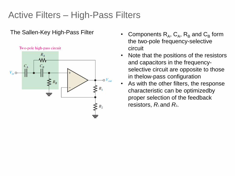
The Sallen-Key High-Pass Filter • Components RA, CA, RB and CB form
the two-pole frequency-selective
circuit
• Note that the positions of the resistors
and capacitors in the frequency-
selective circuit are opposite to those
in thelow-pass configuration
• As with the other filters, the response
characteristic can be optimizedby
proper selection of the feedback
resistors, R1 and R2.
Active Filters – High-Pass Filters

Cascading High-Pass Filters
Active Filters – High-Pass Filters

Active Filters – Band-Pass Filters

Active Filters – Band-Pass Filters

Multiple-Feedback Band-Pass Filter
• The two feedback paths are through R2
and C1
• R1 and C1 provide low-pass response
• R2 and C2 provide high-pass response
• Maximum gain, A0, occurs at the center
frequency
• Q values of less than 10 are typical in
this type of filter.
R1 and R3 appear in parallel as viewed from the C1 feedback path (with the Vin
source replaced by a short).
Active Filters – Band-Pass Filters

• A value for the capacitors is chosen
and then the three resistor values are
calculated to achieve the desired
values for f0, BW, and A0
• Q = f0/BW
• Resistor values can be found using the
following formulas (stated without
derivation):
• For denominator of the expression
above to be positive, A0<2Q2
• => a limitation on gain.
Active Filters – Band-Pass Filters

Active Filters
State-Variable Filter
Consists of a summing amplifier and two op-amp integrators
Integrators act as single-pole low-pass filters combined in cascade to form a
second-order filter
Although used primarily as a band-pass (BP) filter, it also provides low-pass
(LP) and high-pass (HP) outputs

State-Variable Filter
• At input frequencies below
fc, input signal passes
through the summing
amplifier and integrators
and fed back out of phase
• Thus, the feedback signal
and input signal cancel for
all frequencies below fc. • At higher frequencies, feedback signal
diminishes, allowing the input to pass through to
the band-pass output
• As a result, BP output peaks sharply at fc• Stable Qs up to 100 can be obtained
• Q is set by the feedback resistors R5 and R6
according to equation:
Active Filters – Band-Pass Filters
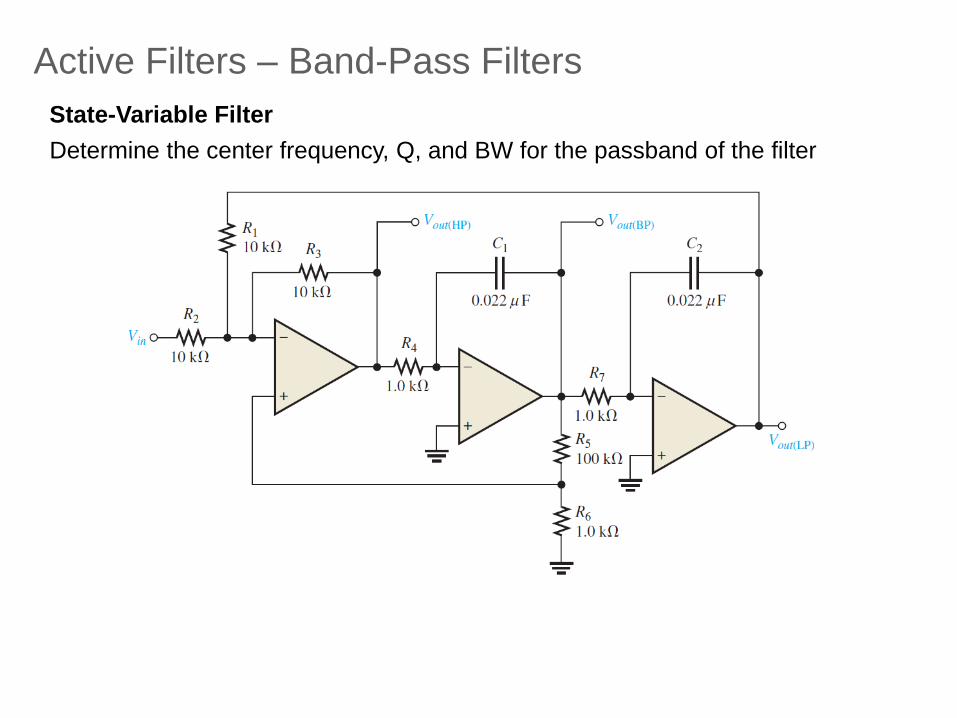
State-Variable Filter
Determine the center frequency, Q, and BW for the passband of the filter
Active Filters – Band-Pass Filters
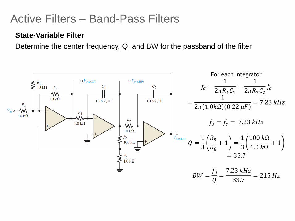
State-Variable Filter
Determine the center frequency, Q, and BW for the passband of the filter
For each integrator
𝑓𝑐 =1
2𝜋𝑅4𝐶1=
1
2𝜋𝑅7𝐶2𝑓𝑐
=1
2𝜋 1.0𝑘Ω 0.22 𝜇𝐹= 7.23 𝑘𝐻𝑧
𝑓0 = 𝑓𝑐 = 7.23 𝑘𝐻𝑧
𝑄 =1
3
𝑅5𝑅6
+ 1 =1
3
100 𝑘Ω
1.0 𝑘Ω+ 1
= 33.7
𝐵𝑊 =𝑓0𝑄=7.23 𝑘𝐻𝑧
33.7= 215 𝐻𝑧
Active Filters – Band-Pass Filters

Multiple-Feedback Band-Stop Filter State-Variable Band-Stop Filter
One important application of this filter is
minimizing the 50 Hz “hum” in audio
systems by setting the center frequency
to 50 Hz
Active Filters – Band-Stop Filters

State-Variable Band-Stop Filter
Verify that the band-stop filter in Figure 15–26 has a center frequency of 60 Hz,
and optimize the filter for a Q of 10
Active Filters – Band-Stop Filters

State-Variable Band-Stop Filter
Verify that the band-stop filter in Figure 15–26 has a center frequency of 60 Hz,
and optimize the filter for a Q of 10
𝑄 =1
3
𝑅5𝑅6
+ 1
𝑅5 = 3𝑄 − 1 𝑅6Choose 𝑅6 = 3.3 𝑘Ω
𝑅5 = 3 10 − 1 3.3𝑘Ω= 95.7 𝑘 Ω
For each integrator
𝑓𝑐 = 𝑓0 =1
2𝜋𝑅4𝐶1=
1
2𝜋𝑅7𝐶2𝑓𝑐
=1
2𝜋 12𝑘Ω 0.22 𝜇𝐹= 60 𝐻𝑧
Active Filters – Band-Stop Filters