ad-777 241 t. p. mcgarty · ad-777 241 models of multipath propagation effects in a ground-to-air...
TRANSCRIPT

AD-777 241
MODELS OF MULTIPATH PROPAGATION EFFECTSIN A GROUND-TO-AIR SURVEILLANCESYSTEM
T. P. McGarty
Massachusetts Institute of Technology
"Prepared for:
Electronic Systerms DivisionFederal Aviation Administration
25 February 1974
DISTRIBUTED BY:
National Techncal Infiuatin serviceU. S. DEPARTMENT OF COMMERCE5285 Port Royal Road, Springfield Va. 22151
.I, ,

TECHNICAL REPORT STANDARD TITLE PAGE
I. stowt No. J2. Gov w Accession Me. 3. Roclo•et's Ceteael No.
ESD-TR-74-40
4. Title mad Subtitle S. Report Da-*
Models of Multlpath Propagation Effects in a Ground-to-Air 25 February 1974
Surveillance Systeem 6. Pw*eiun Orpgeazejon Ce&
7. Aueot(s) I. Peodomnia Organizaeti• Report No.
T.P. McGarty TN 1974-7
9. P*erfomn Oroanizetioe Name and Address 10. WeAA "it No. (T'lJS) 4S364
Mas,-.chusetts Institute of Technology Project No. 034-241-012litxoli Laboratory 11. Contract or Grant No.P.O. !;ox 73 DOT-PA-72-WAI-261Lexington, Massachusetts 02173 13. Type of Report and Period Covered
12. Sponsoring Agency New. and Adess
Department of Transportation Technical NoteFederal Aviation AdministrationSystems Research and Developm~enr Service 14. s oWashington, D.C. 20591
15. Supplementory Notes
The work reported in this document was performed at Lincoln Laboratory, a center for research operatedby Massachusetts Institute of Technology under Air Force Contract F19628-73-C-W002.
16. Abstract
I!
Models are developed for the electromagnetic propagaton of diffuse and specular multipathfor a surface-to-air ATC radar beacon link. The models take Into account geometrical, topographical,electrical, and surface characteristics of the muldpath propagation e-nvironment. The models areused to evaluate signal fading and azimuth estimation performance of a monopulse processor in aground-based interrogator. The results are applied to assessing the performance of die DABS sensor.Conclusions and recommendations for experimental weirk are presented.
DDC ,Reproduced by
NATIONAL TFCUNICALINFORMATION SERVICEU S Department of CommeLrce
Springfe,-I VA 22151
" 17. Key Wors 141, Diutribution Statement
Multipath; Diffuse and Specular Document is available to the publicChannel Cbaracterization through the National TechnicalElectromagnetic Propagation Information Service, Springfield,Antenna Performance Virginia 22151.
It. Security Clessif, (of thise reort) M.Secuirity Cloeolf. (of this pope) m.e. of "Ies 22. Prig*
Unclassified J Unclassified 158 1.45 MF
Form DOT F 1700.7 (1-6a) 4 ALR FRCE: 37360 4/5"174-445
"'.., ,. . o . , . ....:..

TABLE OF CONTENTS
Section Page
I INTRODUCTION ........... .......... 11. 1 REPORT OUTLINE ......... 2
2 FUNDAMENTAL PHENOMENOLOGY . . 52.1 SENSOR GEOMETRY ........ 52. 2 SIGNAL MODEL ........ ........ 11
3 SPECULAR MULTIPATH .......... 183.1 GEOMETRICAL CONSIDERATIONS. 193.2 REFLECTION COEFFICIENT. . . 27
3. 2. 1 Fresnel Reflection Coefficient • 293. 2. 2 Diffuse Reflection Cnefficient • 303. 2. 3 Diffraction Effects ..... 32
3.3 EXAMPLES OF RECEIVED SIGNALS . 423.4 CONCLUSIONS ............. 50
4 DIFFUSE MULTIPATH ............ .. 634.1 THE SIGNAL MODEL ......... 654.2 THE CHANNEL SPREAD FUNCTION 704.3 PERFORMANCE ............ .. 1024.4 CONCLUSIONS ....... .......... 110
5 OTHER EFFECTS ............... . 1135.1 REFRACTION ............. 1135.2 SHADOWING ... .......... 1145.3 SEA SURFACE SCATTERING . . . 1175.4 COMPOSITE SCATTERING 1.......1205.5 CONCLUSIONS. . . . ............. 120
6 APPLICATIONS ..... ........... 1236.1 PERFORMANCE ............ .. 123S6.2 LOCALIZATION ......... 1246.3 ANTENNA DESIGN . .. .. .R...... 1260.4 SIGNAL PROCESSING .. . . . . . 1306.5 SITING........... .......... 1306.6 CONCLUSION•S ............. 130
Precedlig page blank
"V 46.

TABLE OF CONTENTS (Continued)
Section Page
7 CONCLUSIONS ........... ............. 132
APPENDIX I .... ............... ... 135
GLOSSARY OF TERMS ...... ......... 139
REFERENCES ....... ............ .. 145
LIST OF ILLUSTRATIONS
Figure Page
1 Geometry of Canonical Coordinate System. . 7
2 Scattering Plane Geometry ... ....... .. 9-10
3 Ray Optics Propagation Geometry ........ .. 12
4 Diffuse Multipath Reflection ... ........ .. 14
5 Definition of Azimuth and Elevation Angles 16
6 Image Antenna Geometry in Scattering PlaneCoordinate System .... ............ .. 21
7 Azimuth -Elevation Calculation .. ............. 24
8 Geometry of Scattering Angle .... ....... 26
9 Arbitrary Scattering Angle Geometry . 28
10 Reflection Coefficient . .. . .. .... 31
11 Behavior of Diffuse Reflection Coefficient. . . 33
12 Diffraction From a Rectangular Plane ... 34
13 Movement of Diffraction Plane and SpecularDiffraction. . . . . . . . . . . . 35
iv
/_/

LIST OF ILLUSTRATIONS (Continued)
Figure Page
14 Wavefront Propagation .......... . 37
15 Sketch of Diffraction Pattern ......... ... 38
16 Geometry of Fresnel Zones ... ....... .. 40
17 Charleston, S.C., AN/FPS-27 Site 1,000 ftFlight Test Results on 253.6-D1tgree Radial . . 44
18 Geometry of Reflecting Plane for CasesDiscussed .... ............. 46
19 Beam Power vs Inverse Range; Case I . ... 47
20 Estimated Angle vs Range; Case I ...... .... 48
21 Multipath Test vs Range; Case I. . . . .. . 49
22 Beam Power in dB vs Range; Case . 51
23 Monopulse Azimuth Estimate; Case II ..... . . 52
Z4 Multipath Detector Output; Case IJ ........ . 53"
25 Signal Power vs Range; Case III, No VerticalAperture ............ ............. 54
26 Monopulse Azimuth Estimate; Case III, NoVertical Aperture ..... ............. . 5.
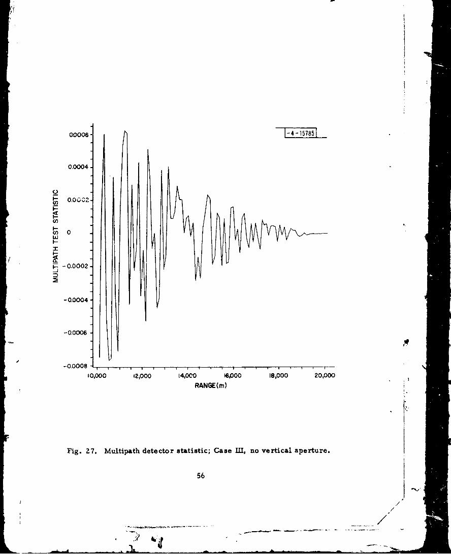
27 Multipath Detector Statistic; Case III, NoVertical Aperture ..... ............ .. 56
28 Signal Amplitude -s Range; Case III, VerticalAperture. . . . . ............ . . 57
29 Monopulse Azimuth Estimate; Case m,Vertical Aperture .... ............ ... 58
30 Multipath Detector; Case III, VerticalAperture. . . . ................ 59
31 Diffuse Multipath Geometry ...... . . 66
V• -1- S,,
N-4

S:.-_
LIST OF ILLUSTRATIONS (Continued)
Fgure Pae
32 Geometry of Receiving Aperture . ..... 68
33 Geometry of Direct Path ... ........ . 7 _..72
34 Ttme Vari:-tion of Area ............. ... 74
35 Area, S(t), vs time (z1 = 1Oin, Z= 3 km,R -L 5kin) ..... .............. ... 77
Vn
36 Differential Area vs Time (S(t + T) - S(t);T= 1 sec; z 101m, z 2 = 3kn, R= 15km). 79
37 Differential Area vs Time (S(t = T) - S(t);T= 1.6 sec;z,= 10M, z2 = 3km, R= 13kkm) 80
38 Scattering Geometry. . . . . . . . . . . 81
39 Scattering Cross-Section vs Azimuth
( = 88o,= 1/2) ...... ......... 86
40 Scattering Cross-Se tion vs Azimuth(ýi = 0s 880, s = 1/2 ). .......... .. 87
41 Scattering Cross-Section vs- AzimuthI88o, s = Z) . . . . . . . . . . . 88.
42 Scattering Cross-Se9tion vs Azimuth(41 = 9 =88o, = °2) . . . . . . . . . 89
43 Spread Function Geometr,. .......... .. 9110"
44 Scattering Geometry .................. 93
45 Contour Plot of Scattering Cross -Section(R= 1O kin, z2= I km, s = 0.5) .... ...... 96
46 Contour Plot of Scattering Cross-Section(R= 50km, z,= I km, s = 0.5) . . . ... 97
47 Contour PloW of Scattering Crobs-Section(R= 50kkm, z = I km, s = Z. 0 ..... 98
48 Contour Plot of Scattering Crobl-•actan=.(R= 50 kin, z l km s= 4. O) ....... .... 99
Vi
__/-. -.. -

- J=
LIST OF ILLUSTRATIONS (Continued)
Figure Page
49 Plot of Channel Spread Function vs Azimuthfor Two Correlation Lengths ....... .. 101
50 Plot of Multipath Energy to Signal vs Range . 103
51 Standard Deviation of Angle Estimate . . . 108
52 Plot of Aircraft Altitude vs Maximum Range%. Horizon ............ ............. 115
53 Model of Ocean Waves ... ........ .. 118
54 # Real Part of Fourier Transform ..... 127
55 Imaginary Part of Fourier Transform . . 128
56 Power Spectrum ... ........... 129
VU

SECTION ONE
INTRODUCTION
As a signal is transmitted from one point to another above a surface
with electrical properties differing from that of the propagation medium,
reflected signals may be generated. These signals then appear, along with
the signal travelling over the direct path, at the receiver. These additional
signals directly affect the communication and direction finding capabilities of
a surveillance link operating in this environment. These signals are corn-
monly called multipath and it is the purpose of this report to describe models
of such phenomena that are useful for ascertaining the efficacy of such a link
for surveillance.
Specifically, the models developed are to be used to evaluate multi-
path effects on the DABS (Discrete Address Beacon System) performance.
For this system, a downlink receiver (sensor) is tn the surface and the trans -
mitter is located in an aircraft. Clearly, due to reciprocity, the role of the
transmitter and receiver can be interchanged but, in this report, we shall use
the stated nomenclature. The link being discussed is one where the receiver
is close to the ground (5-50 m high) while the transmitter is at a highr- alti-,: tudes (500-15, 000 m) and the range bs large (10- 100 kin). This is in contrast
to ground-to-ground or air-to-air links as found in mobile radio or satellite
communications respectively.
What we shall do in this report is consider those effects which are
relevant to the ground-to-air environment and develop models which are -
"'-C

appropriate. Our interest will not be in the microstructure of diffraction
effects due to specific structures but will be towards developing models that
* can be easily used to evaluate the multipath effects on system performance.
Namely, we shall be interested in the general macrostructure of the multipath
environment.
The two main functions of this report are:
I. Model DescrIntion: In this area. we evaluate the topo-
graphical, geometrical, electrical, and system para-
meters and how they affect the RF signal at the receiv-
ing antenna. Specifically, specular and dffuse multi-
path are discussed in detail in terms of the above
parameters.
2. System Performance: Once the multipath model has
been developed, the effects of the multipath signal on
the SNR (signal-to-noise ratio) and direction finding
capabilities of a monopulse antenna with a 20 beam-
width and vertical sector beam are ascertained.
1.1 REPORT OUTLINE
In Section 2, we discuss first the goometry of the aircraft and the
sensor by introducing a canonical coordinate system. The large scale topo-
graphic features such as hills, buildings, etc. are then defined in terms of
this coordinate system. We then proceed to discuss the difference between
specular and diffuse multipath and the surface conditions that give rise to
each of them. A model of the RF envelope of the receiving antenna output is
presented. This equation is the basis for the multipath model development.
2
/
S......... : '............ ... . ... . ... . '••--• •., ..- ,• _ - •'=:'r= ... .•: ... .

Section 3 discusses the nature and effects of specular multipath on
the received signal. Using the geometrical models developed in Section 2,
a geometrical optics analysis of specular reflections is developed. The path
length, angle of incidence, azimuth, and elevation of the received specular
multipath signal are determined. Since specular multipath arises from large
" •scale surface areas, the reflection coefficient is studied in detail. The effects
of electrical properties at the reflecting surface, finite aperture diffracti.on and
losses due to diffuse multipath are considered. The section concludes with a
discussion of the use of the models in the analysis of signal fading and monopulse
azimuth estimation. These issues are related to the performance of DABS.
The model for diffuse multipath is developed in Section 4. In contrast
to specular multipath, which is a highly deterministic phenomenon, diffuse
multipath is random in nature. To account for this, a model is developed
for the second order statistical properties of the multipath field. A function
called the channel spread function is introduced. The spread function is then
evaluated in terms of the surface properties using the Kodis-Barrick scatter-
ing cross-section model. Section 4 concludes with a discussion and evaluation
of the effects of diffuse multipath on azimuth estimation performance. It is
shown that there is a negligible effect in the DABS case.
Section 5 discusses other effects that, although not included in the
models, may in time be important. These elfects include refraction, line -
of-sight limitations, 5hadowing, sea-surface scattering, and composite
scattering.
Z•; The last major technical section is Section 6. Here we discuss the
various applications to which the models may be put to use. Specifically,
3

we mention link and azimuth estimation performance and localization techni-
ques. Also discussed are antenna design, signal processing, and siting.
The conclusions of the report are detailed in Section 7. Basically,
we show that DABS should function acceptably based on the multipath model
developed in this report. We also comment on the other uses of the model
and briefly on its shortcomings.
i
* * !
wŽ
4
I4i

- . . . ...%W t, V .wm . . .. ... -
SECTION TWO
FU NDAMFNTAL PHENOMENOLOGY
In order to fully understand the effect of multipath on the energy
received at an antenna aperture, it is first necessary to describe the total
S . environment in which the signal transmission is taking place. This envito)•tncnt
includes the reflection geometries involved between transmitter and re.'
the nature of the wzveform transmitted and the effects of the receive'r:- antenna
on the received signal energy. In this section we shall treat each of these
issues separately and on a level which will provide the reader with a qualitative
as well as quantitative understanding of the problems involved.
2.1 SENSOR GEOMETRY
The basic geometry of the aircraft and DABS ground receiver is
quite simple. In order to avoid certain analytical problems we shall first
assume that we have a flat earth. Let us then choose a point 0 on the earth
plane and at this point construct a set of three orthogonal axes, one being nor-
mal to the plane. This will b, defined as the canonical coordinate system and
will be used throughout the report. The interrogator antenna DABS sensor is
* located at an altitude z above the origin. This point represents the phase
or geometrical center of the antenna. It is that point to which all phase delays
a are referenced. The earth plane is designated the x, y plane and in this con- I
text, the antenna coordinates are (0, 0, z1 ). The aircraft is at an altitude
j5

z above the plane and at position x2 and y 2 on the plane. Thus, the aircraft'c
position is (x 2, Y2, La). The range from the antenna is given by RT where
2 2+2 1/2(21RT =[(z•-zl2 ]) + . . i_2
This geomet-y is shown in Fig. I. Another important constant is
the ground range R where
2 2 1/R[x 2 + y 2
Actua)ly, the earth's surface is not a flat plane but contains hills and
other large obstructions such as buildings and bridges. These may be con-
sidered large scale surface perturbations, being the size of many wavelengths
of the transmitted radiation. There are also small scale obstructions such
as 3mall rocks, trees, grass, water, roadway surfaces, etc. which are in
size less than several wavelengths. it is necessary to consider both of
these classes of obstructions in any model. In many cases, the large scale
obstructions are limited in number and are easily defined and characterized.
For example, a large hill can be easily identified from a topographic map.
However, the small scale obstructions are quite numerous and detailed in
their shape as compared to a long smooth hill. Thus, the large scale obstruc-
tit as are often amenable to a deterministic analysis whereas random analyses
are necessary for the understanding of the small scale effects. Thus, we
shall leave discusslon of the latter to Section 4 and consider the former here.
J I

TRT AIRCRAFT
ANTENNA I
0 1i
X2 ---- - - - - -
&m
Fig. 1. Geometry of canonical coordinate system.
P.
il

We shl1l assume that any lage scale obstructions can be represented
as a suitably sized section of a plane that has been positioned to coincide with
the actuai obstruction. For example, if there is a large building parallel to
the y axis in Fig. 1, then it can be represented by a plane of equivalent size
and electrical properties located at the same position. These equivalent
planes will be defined relative to the canonical coordinate system.
A model of the scattering surface is constructed in the fashion shown
in Fig. 2. From the canonical system we displace another orthogonal coordi-
nate system (x', y', z') by a vector E0 (Fig. Z(a)). Then this system is rotz ted
about the y' axis by an angle a (see Fig. 2(b)) called the cross-range tilt. It
is called cross-range because the y-axis is usually associated with the hori-
zontal range and nmultipath reflections from such a tilted surface will cause
monopulse azimuth e-rurs in the cross -range direction. The resulting coor-
dinate system x", y", z" (Fig. 2(b)) is then rotated about x" to an angle (•
(see Fig. 2(c)) yielding a final coordinate system x"', y"', z"'. # is called
the range tilt angle. Finally, in this coordinate system on the x", y"' plane,
we define a surface S (see Fig. 2(d)) as the scattering surface. In this fashion
we can construct a set of contiguous surfaces which represent the large scale
surface topography and present a one-to-one mapping of the large scale sur-
face topography. In the next section we shall partAcularize this further in the
study of specular reflections. We shall also see in Section 4 that surface
roughness, namely small scale surface irregularities, can be included
direc:tly by superposition.
8
a-. -'-

_ro .- - -.--- y' -----------..--.--. ,.- - -,.------
zz
x
(a) Origin Displacement
z i
Z aX11
y
x (b) Cross-Ronge Tilt
Fig. 2. Scatter'.ng plane goemetry.
9
' i
__ _

zz 118-4-162131
Z111 y
y
Wc Range Tilt
z
-SCATTERING SURFACE S
y
( Scattering Aperture
x5
Fig. 2. Scattering plane goemetry (Continued).
10
-
A I'

2.2 SIGNAL MODEL
Now, with the description of the geometry of the environment, it is
possible to discuss the nature of the signal propagation. We shall concen-
trate on the signal transmitted by the aircraft and received by the sensor
antenna, which we term the downlink signal. For large scale irregularities,
such as hills, we cau use the simplifying analytical techniques of ray theory
to determine the propagation of the electromagnetic energy from the transmit-
ter to receiver. For example, in Fig. 3, we depict the aircraft at T and the
receiver at R. We assume that the x, y plane is the surface of the flat earth
model and that S is .;eparate large scale scattering surface. The points P
and G are the reflection points on these two surfaces. Path T is called the
direct propagation path and represents the free space propagation from T to
R. Path ®•, TGR, is the ground propagation path with reflection point G.
The reflection point is determined directly from the image antenna at R'.
Path 3, TPR, is what we shall call a multipath signal return. It is a sig-
nal return that results from other than flat earth reflections. It is this type
of return that proves to be most detrimental to direction finding (DF) accuracy.
The signal returns in Fig. 3, are clear, well defined signals which
appear at the receiver as signals coming from directions other than the direct
propagation path. Such strong well defined returns are called specular mul-
tipath and result from large reflecting surfaces such as buildings and hills.
A second kind of multipath signal, called diffuse multipath, occurs due to the
small scale surface irregularities. Obstructions such as trees, windows,
rocks, and other "small" obstructions cause multipath returns to appear to
11i
-ll-

z
S4
!Z2
2y
II
I
I i
Gl
9 *1
y£
x118-4-5,1:
Fig. 3. Ray optics propagation geometry.
'a1
,9i
- ~ - -K

come from a spectrum of directions instead of a single well defined direction.
An example of such a phenomenon is shown in Fig. 4 where we depict many
small reflectors. Diffuse multipath is a random phenomenon as a result of
large number of objects giving rise to it. As such, an analysis of its effect
must be phrased in terms of these random orientations. Furthermore, the
analysis of diffuse multipath effects requires the inclusion of diffraction
phenomena and cannot be performed using classical ray optics techniques..
To observe the effects that these different phenomena have on the
received signal, a model for such a signil must be developed. In general,
the signal will be narrowband, centered about a carrier frequency Wc" We
assume that the transmitter emits a spherical wave from an omnidirectional
antenna (variations from which will be considered later) having a time varia -
tion of the form,
s(t) = Z Re[s(t) exp.j~ct)] (2.3)
The tet:m ;(t) is the complex envelope of the signal and has the form
+* (t) F--S 1(t) (2.4):'
where E. is the signal energy and f (t) is a normalized version of the temporal -
variaticn. Namely,
ft * (t) f dt - (2.5)
13

Z 118- 4- 157621.
T
*R
~ i
Fig. 4. Diffuse multipath reflection.
14
~1 , i.
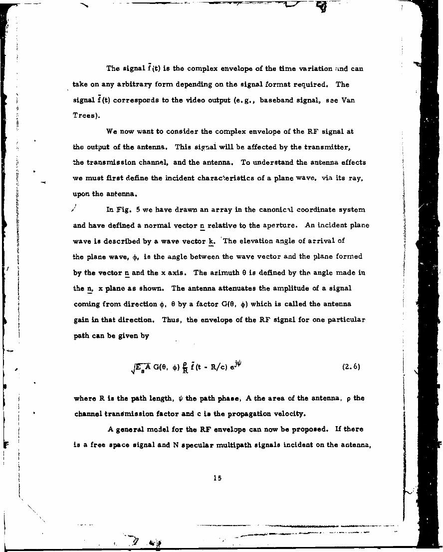
The signal 1(t) is the complex envelope of the time variationa;nd can
take on any arbitrary form depending on the signal format required, The
signal f(t) corresponds to the video output (e.g., baseband signal, see Van
Trees).
We now want to consider the complex envelope of the RF signal at
the output of the antenna. This signal will be affected by the transmitter,
the transmission channel, and the antenna. To understand the antenna effects
we must first define the incident charac.eristics of a plane wave, via its ray,
upon the antenna.
In Fig. 5 we have drawn an array in the canonical coordinate system
and have defined a normal vector n relative to the aperture. An incident plane
wave is described by a wave vector k. 'The elevation angle of arrival of
the plane wave, ý, is the angle between the wave vector and the plane formed
by the vector n and the x axis. The azimuth 0 is defined by the angle made in
the n, x plane as shown. The antenna attenuates the amplitude of a signal
coming from direction ý, 6 by a factor G(O, 0) which is called the antenna
gain in that direction. Thus, the envelope of the RF signal for one particular
path can be given by
FTG(O9 *i(t - R/c) ejo (2.6)
where R. is the path length, ~Pthe path phase., A the area of the antenna, p the
channel trandmission factor and c is the propagation velocity.
A general model for the RF envelope can now be proposed. If there
is a free space signal and N specular multipath signals Incident on the antenna,
15
I$I
.~ 'ii

22
CANON ICALioCOORDINATE
x
Fig. 5. Definition of azimuath and elevation angles.
16
Al2

plus diffuse multipath and noise, then the received signal is given by;
SN
r(t) - r G(Oi, i) (t Ri/c) exp(joi)
i=O _
'+ G(O, (e, ,,t) dedý + .(t) (2.7)+._-
Here 0i, 0i are the azimuth and elevation of the ith specular signal and pi' R.I
and 0i are the transmission gain, range and phase respectively. The i=O terms
correspond to the free space path. The term b(O, 0, t) represents the effectsof diffuse multipath to be discussed in Section 4. The noise i(t) represents
all noise not attributable to signal transmission observed at the RF output.
One of the purposes of this report is to describe how one can evaluate
all of the terms that appear in this expression and show how they relate to
the actual terrain topography. For example, the quantity p will depend on
reflection coefficients, diffraction effects, diffuse reflection effects, as well
as the vagaries of the transmitting antenna. Tho term b(O, 0, t) is a random
process imbedded in a random field. The evaluation of its statistics is quite
involved and will require some detailed knowledge of the surface topography.
IF
177
•.77 f m m m

SECTION THREE
SPECULAR MULTIPATH
The dominant multipath effect in terms of direction finding and com-
munications in the DABS environment is specular multipath. As we shall see
in the next section, diffuse multip th plays a second order role which, though
marginally important, does not limit the performance of the DABS system.
Specular multipath is felt in terms of signal fading and azimuth estimation
errors. It can be analyzed deterministically for each specific geometry or
probabilistically for an ensemble of such geometries. It has been found that
a deterministic analysis provides greater insight into how it can affect system
performance. In this section we shall concentrate on a deterministic analysis
and briefly comment on proposed random models.
As introduced in the last section, the direct tree space signal pluse
the specular signal received at the RF output of the antenna is given by
E~sA G(0i ýi) R• exp[jo,] (.,il_
i=oi
where i=O corresponds to the direct path ray. The problem is to determinis-
tically evaluate 01, 01, Pi' Ri and 0 for each of the rays. This is to be done
knowing the number of scatterers, the surface geometry, the antenna pattern,
the aircraft position and the electrical prcnerties of the surface.
18- *. -- nn-

-
3.1 GEOMETRICAL CONSIDERATIONS
To evaluate these quantities, we must first further quantify the geo-
metry. Let us assume that the receiving antenna is an array and the phase
(geometrical) center of the array is at some vector rl where
xl
SY(3.2)
rL U
which is a generalization of the definittion of Section Two. Likewise, assume
the aircraft is at r 2 where
1!
=Y2 (3.3)
Both of these vectors are defiled relative to the canonical coordinate system
developed in the last section. Now we w-i, -.,e •he itI. scattering plane (I - 2)
as the septuple Pt of surface area Sip, T1,h nt.ts oi. ýj(i - 2) where;
P k1 i= cxip 0i' Sip EJ) Ti, Trs (3.4)
Here, Eo is the offset vector of the ith scattering plane (see Fig. 2), and
(i are the dielectric constant and conductivit :)f the plane. Ts is the surface
roughness coefficient as obtained for diffuse multipath effects. This septuple
completely defines the scattering plane and will provide all the information
19
4j1

necessary foT our model of the channel. Given the antenna gain, the received
siglai is completely defined.
We shall proceed by first determining Ri the range between the trans-
mitter on the aircraft and the receiver via the ith multipath source. We shall
briefly outlive this derivation and present the result. When using a ray optics
approach the point of reflection from the ith surface is dete~rthined by extend-
ing the ray from the source to the image antenna. The image antenna is de-
fined as being that point relative to the scattering plane (Xi', ytt plane) which
is equidistant from the opposite side of the plant as die receiver and lying on
the normal created by the receiver and the scattering plaLt. For example, in
Fige 6 we have depicted an antenna at R in the y, z plane and a transmitter at
T also in the y, z plane. The image antenna, since the x, y plane is the scat-
tering plphe, is at the point R. The line RO is normal to the x, y plane.
The length of the path is T9+ M or equivalently TR'W. The vectorr is the
vector from the origin to the image antenna. What should be noted in this
figure is that since the x, y plane is the scattering plane and the image
antenna lies along the normal RO at the same distance from the x, y plane
as r1,then -ihas the same x, y coordinates are rand a z coordinate
that is the reegtive of r This then suggests how the image antenna for the
igh scattering plane can be obtained. Namely, translate and rotate the coor-
iiT lso in the y, replatie. tohe caoicage systemn , usinge the xypand and tes -
ploy the algorithm suggested above. Then retranslate and rltate back to the
canonical coordineate system. Doing this we find that the position of the iiage
antenna in the canonical coordinate system is given byfr where
i
as rl, hen '• as te sme x y zooriae r 1adazcodnt
" ... Ia i h .e-ieofr.Tiste uget o th image anenafIth

T
R ANTENNA /
0--- S REFLECTION POINT Y
R-IMAGE
Fig. 6. Image antenna geometry in scattering plane coordinate system.
21L p. i\\*-. ~ ~

_( - + (3.5)-
where is the matrix which performs the above mentioned operations. The
entries of are;
- 2 2 2 2Cos a1 - sinsi~n sin2gi sin2aicos (
= sini sin2gi • cos2(3 cosmsin2(3.
2 sn.•2 2-sin2a_ Cos 3 co sin s a - cos acos2
(3.6)
Thus Ri. the path length, via the ith multipath reflector, is deter-
mined by
R ri = [(12- !it) T(!12 - r 1/2 (3.7)
This is the value of Ri used in (Z. 7). Now 'Pi represents the phase of
the ith path. If we arbitrarily define 00 then
(R1 - R 0 )S00o + ZW + F. (3.8)
where X0 is the frce space wavelength and R is
- T - ]1/2R- . 13.9)
I.F
m / ',,L ••

The term R. is the phase of the ith reflection process which we shall define1.
shortly (see 3. 2. 1).
In a similar fawhion, we can use this formalism to evaluate the azi-
muth and elevation (9 ) of the ith multipath source. Consider the geome-
try in Fig. 7(a). The xy plane is the reflection plane which contains a point of
reflection, S. Note that at the point S the ray changes direction and is reflected
to the antenna. The azimuth and elevation are then defined relative to the
vector that represents the scattered wave. Let us call that'vector r NowI
r relative to an arbitrary shift of coordinates is equal to the vector s, thei
incident vector, except that the z coordinate has its sign changed. From the
geometry, s. is given by
-. - . (3. 10)
We can normalize st so that it has unit length. This is defined as the vector
where;
!2rrz -r'i (3.11)
Consider Fig. 7(b). Here we depict yi, the scattered version of The
elevation of the multipath relative to the array is defined as - €j, as shown,
and the azimuth is - 0 as shown. Thus ý,' and 0, are easily obtained by know-
ing the components of r which are directly obtained from !L as described."--i
This technique can then be extended to any arbitrarily rotated plane
following the reasoning developed before. Namely, can be shown to be;
23

r2r
R y
If
Fig. 7. Azimiut h-elevation calculation.
24
iiVm e le
- -~SIM~r4ill.•mIk
•s-4-•ssl i,,
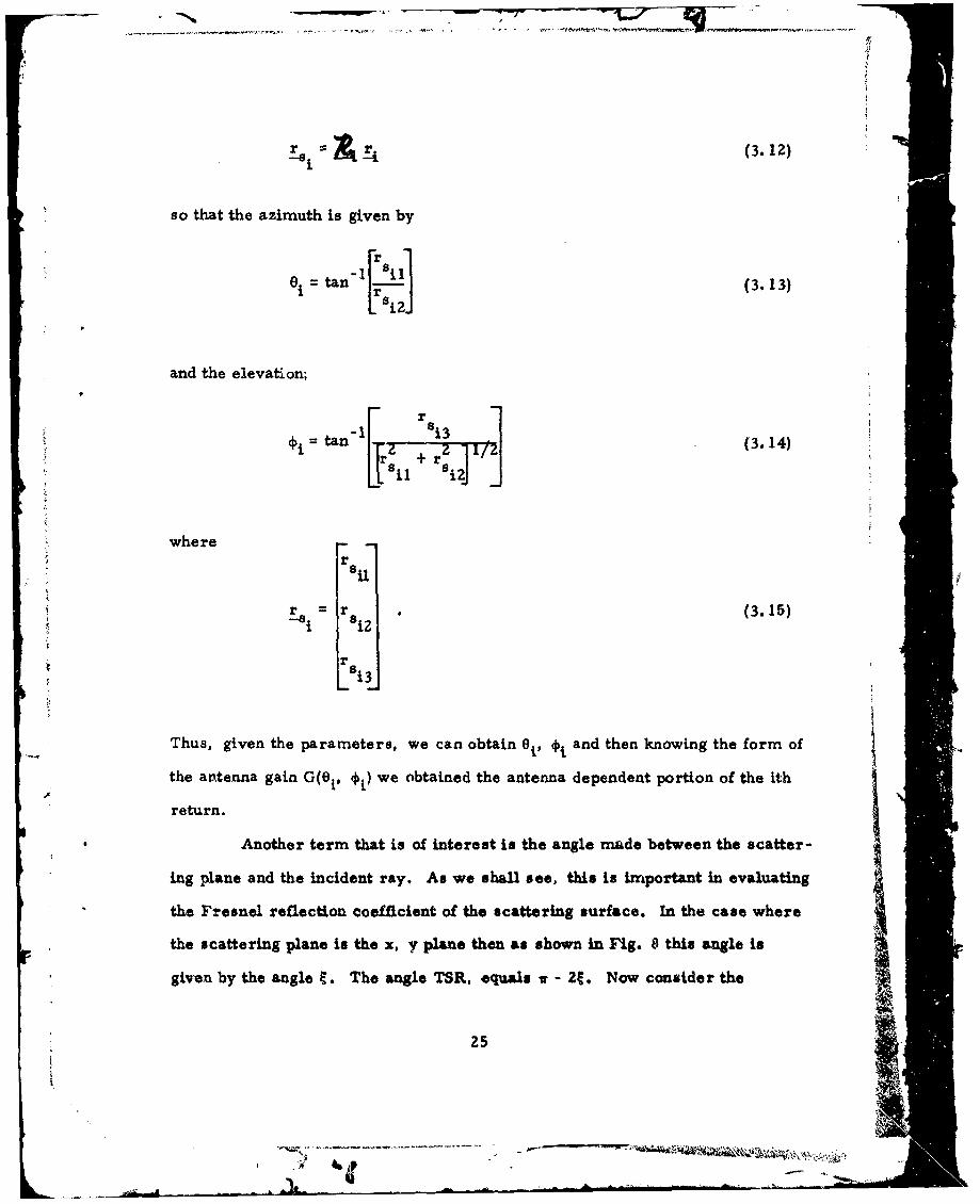
t "(3.12)
so that the azimuth is given by
0 tan (3. 13)
S rSi 3
S~~where --rr31
I i2
r si3
Thus, given the parameters, we can obtain 0U, 0" and then knowing the form of
the antenna gain G(Ot, *,) we obtained the antenna dependent portion of the Ith
return.
r r Another term that is of interest is the angle made between the scatter-
ing plane and the incident ray. As we shall see, this is important in evaluating
the Fresnel reflection coefficient of the scattering surface. In the case where
the scattering plane is the x, y plane then as shown in Fig. 8 this angle is
given by the angle •. The angle TSR, equals v - 2. Now consider the
25

T
R
C/
.1 4
Fig. 8. Geometry of scattering angle.
26
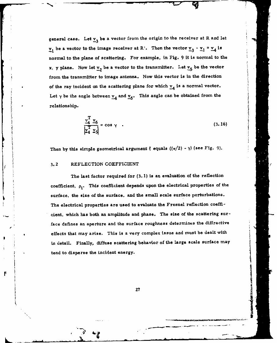
general case. Let Y3 be a vector from the origin to the receiver at R and let
xI be a vector to the image receiver at R'. Then the vector v - vI = v is
normal to the plane of scattering. For example, in Fig. 9 it is normal to the
x, y plane. Now let v be a vector to the transmitter. Let v 5 be the vector
from the transmitter to image antenna. Now this vector is in the direction
of the ray incident on the scattering plane for which y4 is a normal vector.
Let y be the angle between y4 and •-5 This angle can be obtained from the
-i relationship.
• T= cos Y (3.16)
Then by this simple geometrical argument 9 equals ((w/Z) - y) (see Fig. 9).
3.2 REFLECTION COEFFICIENT
The last factor required for (3. 1) is an evaluation of the reflection
coefficient, p1. This coefficient depends upon the electrical properties of the
surface, the size of the surface, and the small scale surface perturbations.
The electrical properties are used to evaluate the Fresnel reflection coeffi-
cient, which has both an amplitude and phase. The size of the scattering sur-
face defines an aperture and the surface roughness determines the diffractive
effects that may arise. This is a very complex issue and must be dealt with
in detail. Finally, diffuse scattering behavior of the large scale surface may
tend to disperse the incident energy.
F2
1*
- -

IY2
13~
Y3ii V4YI-ii Y5Y J ii
R_ -_
Fig.~~~~~~~~I 9. Arirrectein nl emty
Z8ll
". { m_ ! !ni

.. , I-.-L/¸ W*~ --,SLL , •V*I -o
Considering the above three effects the reflection coefficient, pi,
can be written as;
!!Pi " DF(3.17)
i ii
where YA is the coefficient accounting for the finite aperture effect, n D the
diffuse reflection coefficient and ti the Fresnel reflection coefficient due toF
the electrical properties of the surface.
3.2.1 Fresnel Reflection Coefficient
The Fresnel reflection coefficient YIF and the phase ;P, (3.8), can
be obtained by an analysis of the reflection of electromagnetic waves from
smooth surfaces with known electrical properties. The properties of the
reflector also depend upon the polarization of the incident plane wave. To
simplify the analysis we shall assume a single polarization, vertical, and
avoid until Section 5 any of the problems associated with depolarizing surfaces.
The complote reflection coefficient is a complex quantity Fwi
n = •F exp(jOFi) (3. 18)
It is shown In Jordan and Balmain (p. 631) that for vertical polarisation
jx)-cos ~(3.19)1 (f - ix) sing+ (C ix)-Cos
29
NT 17M• t1

where j equals 4-1 and • is the angle of incidence given by ({w/Z) - y, where
Y is defined in (3. 16). x is
xa (3.20)/eWie
where a* is the reflector's conductivity, w the angular frequency of the inci-
dent radiation and E vthe dielectric constant of the propagation medium. Also-
E r = E/ev (3.21)
where E is the dielectric constant of the scattering surface.
Thus for different electrical surface constants, c and a, values of
nFand 41 F can be obtained as a function of the incident angle 9. Usually 9
is quite small, which means that nFi is close to unity and 0. close to wr.
However, for different surfaces, the behavior of these terms as a function of
Svaries significantly. In Fig. 10 we have shown the magnitude and phase for
a typical surface. It can be seen from Fig. 10 that a significant change in
rFl occurs as 9 increases. Also the dip at the Brewster angle may vary fromIi
a significant drop to only a 3 iB drop in amplitude depending upon the surface
characteristics.
3.2.2 Diffuse Reflection Coefficient
When the surface of the scatterer is rough, energy from the incident
ray is scattered away from the specular scattering direction (and thus is lost
from the received signal). To account for this effect, we introduce the diffuse
30
- - ~ie

1.0 T3356
PHASE
20ii0.2
1. - - 40
0.6 so
40-IQ. AMPLITUDE "-- 80 .9
04 a.0.4- - 100
120
0.2- - 140
- 160
0 9 Is 27 36 4 4 63 72 *
INCIDZNT ANGLE (dog)
Fig. 10. Reflection coefficient.
31

reflection coefficient YD for each surface. This coefficient has been deter-ni
mined by Beckmann [2] and it depends upon the angle of reflection, g, as does
the Fresnel reflection coefficient. It also depends upon the statistical proper-
ties of the scattering surface. Specifically, if z(x, y), the height of the su:--
face at point x, y, is a zero mean Gaussian random variable with variance
S, B eckm ann show s that
ex D . (3.22)i/J
For • close to 0 the coefficient is near unity. However, for very rough
surace (ah» 0),this term decreases rapidly as the angle of inci-
dence increases. In Fig. II we have sketched for two di~erent roughnessDi
ratios, A0h/3, as a function of •.
3.2.3 Diffraction Effects
As the size of the reflecting surface decreases, diffraction becomes
important ,ad ultimately dominates the behavior. For example, it is well
kwown that a rectangular surface illuminated by a plane wave from direction
k as shown in Fig. 12(a) diffracts the radiation into the specular direction and
into other directions according to the sin x/x distribution. In Fig. 12(b) we
have plotted the distributions of the diffracted amplitude of the field in the k,
ky directions. Note the central peak in the specular direction, k', and the
presence oi sidelobes in other directions. In Fig. 13 two representative
specular reflectors, S1 and S., are shown with sketches of the diffraction
pattern of the reflected radiation superimposed. The dimensions of surfaces
32
/i /

• ~~118-4-15.•~
•OrD
SO.D1 <O'D •
{2
Fig 11 Beavo ofdfuerfetinCefcet
0 7T
AP
33
t
"- - .
, .1 •, -

Sz 118--4_15•770
k
(a)
yL
k• y
(b)
Fig. 12. Diffraction from a rectangular plane.
34
-
- .. ... .:A .

N rmz 118 -4-157711I
\T
R\
NVol
\ "
R 52 S, •
Fig. 13. Movement of diffraction plane and specular diffraction.
35
• a - .- -a•,a !
a "

S and S2 are assumed to be small enough that the radius of curvature of the
wavefront is large compared to the surface size. This allows us to say that
the incident wave is coming from the direction joining the midpoint of the sur-
face to T, and the the surface is irradiated by a plane wave.
The amplitude of the field received from a reflector depends on the
width and orientation of the diffraction pattern, which in turn depends on the
size and location/orientation of the reflector, respectively.
From geometrical optics we know that if T emits a spherical wave
and the wave is scattered by some plane, then the s1 .attered wave is also
spherical. Furthermore, the apparent direction of the radiation can be
obtained by observing the direction of the ray passing through the desired
point. Thus, in Fig. 14, we have drawn a ray diagram for a wave travelling
from T aud have shown seven receivers. The reflected wave is also shown to
be spherical by drawing the normal to the rays. Now consider any one of the
receiver points Ri. For this case of an inifinite reflecting plane, we see that
there is a definite reflecting poilit, Pi, at which the ray follows Snells law.
We now pose the question: If there is only a finite amount of scattering sur-
face, and Pi is not on that surface, what is recei-ved at Ri ? To find the
answer we must consider diffraction analysis. Thus, in Fig. 13, if R is in
the sidelobes of that diffraction pattern of surface S1, its amplitude is de-
creased. Furthermore, we can consider the fo.lowing experiment. If we
fix R and T in Fig. 13, move the surface S and plot the amplitude of the
received field as a function of y, the range, we will effectively plot out the
diffraction pattern for that surface. This result is sketck'ed in Fig. 15. When
the surface is centered at a point y*, tL, amplitude of the signal received at
R reaches a maximum.
36
... ,I

l R7 i•-4-157772f35118
Re WAVEFRONT
• • T
'• WAVEFRN
R,- GROUND PLANE
_- , 3e P;.P"" P 7R
r
R -7
Fig. 14. Wavefront propagation.
37
"0-; }. _. ,B.. • . .......
v..•,,:•i , .

Fig. 15. Sketch of diffraction pattern.
38
- -- -- -. -- -.

Now if S is large enough (to have a narrow diffraction pattern) but
not too large (small with respect to the radius of curvature) then the point y*
in Fig. 15 will, in some sense, correspond to the reflection points Pi in
Fig. 14. That is, by positioning this small surface at the right point, we
can effect a received wave that would appear to be coming from an infinite
reflecting plane. This idea is the basis of the Fresnel zone concept. Further- jmore, it can be rigorously shown that if one has many such planes, that only
the one centered at the right position will contribute to the received field
while all others will coherently cancel.
In view of the above discussion, we car, consider what portion of an
infinite reflecting plane dominates in the reflecting process. This area is
called the first Fresnel zone anti represents the region on the plane where
the first ir radians of phase shift occurs. The higher order Fresnel zones
represent regions of increasing ir radians of phase shift. These zones aredepicted in Fig. 16(a). The first zouae is shown in Fig. 16(b) in more detail.__i
It is an elliptical surface located at a center point y0 1 with an extent + A 1
about that point and + xI about the x axis. These quantit~es are given in
terms of z1, Z., and r as follows:
- ZZl(zI + z2
ya1 (3.23)Y0I " (zl + z) (.1
39
- -.. ,v----B..
- ----- ~--•-H-- s

r('
(a)
Al
txl~ -----
Fig. 16 emtyo Fenlzns
1 +
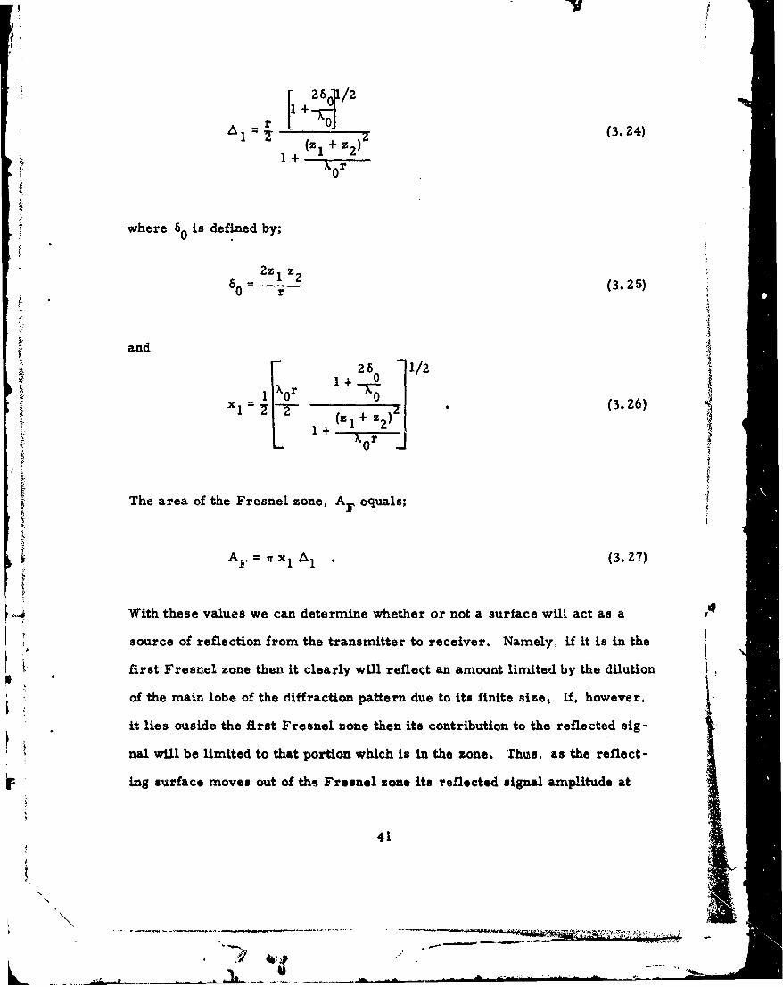
r 0 (3.24)(z1I + z2Z'
S1 + 0r0
where 6 is defined by;
"6 2z 1 z 2 (3.25)
and
26 -1/
__+ 01~ 0 -1ý00
" -(3.26)(z 1+ z2)1+_
0 iThe area of the Fresnel zone, AF equals;
AF= Irx1 1 (3.27)
With these values we can determine whether or not a surface will act as a
source of reflection from the transmitter to receiver. Namely, if it is in the
first Fresnel zone then it clearly will reflect an amount limited by the dilutionI "
of the main lobe of the diffraction pattern due to its finite size, If, however,
it lies ouside the first Fresnel zone then its contribution to the reflected sig-
nal will be limited to that portion which is in the zone. Thus, as the reflect-
ing surface moves out of the Fresnel zone its reflected signal amplitude at
"41
N
-\- -, - - -~-- - .

the receiver decreases, the amplitude being determined by the sidelobes of
the diffraction pattern.
Thas an evaluation of the diffraction reflection coefficient1, . canDi
be determined from the diffractiom pattern of the surface being irradiated.
However, such a calculation is often quite tedious. A reasonable approwdma-
tion is let iD equal the ratio of th, amtunt of reflecting surface area in theIm
first Fresnel zone to the .rea of the first i" resnel zone. This is a quantity
that is easily calculated. That is, if Ai is the area of the ith reflector in the
first Fresnel zone then;
T3 =X .- . (3.28)i F
Thus, (3. 19), (3.22) and (3. 28' provide all that is necessary for pi
in (3. 17). Furthermore, this completes the specifications of ail the para-
meters in the specular signai of (3. 1).
3.3 EXAMPLES OF RECEIVED SIGNALS
The model developed at the beginning of this section for the specular
portion of the received signal can be used to demonstrate the effect of certain
terrains or structures on the signal. The dominant effect is that of fading,
where the direct return and other multipath returns add coherently to cause
a decrease in signal amplitude. This can produce a reduction in the signal-
to-noise ratio which seriously affects detection and position estimation. Using, .
the model just developed, it is possible to see what type of multipath environ-
p ment will give rise to the more deleterious effects and how through proper
siting and antenna design, they may be prevented.
42
. ..........- .- -
- -A

The fading property of the signal is easily observed by evaluating the
power in the specular returns. Thus, let o(t) be the magnitude squared of
(3. 1). It can be written as;
N 2
;(t) E AE G (e1 , *1If~SN N
+EsA N G(0i, *i) G( j, 0j) pipj
1=1 j=1V.jR .
t-* f L iI) L~ (t C_ .(~ (3.29)
Now if f(t) has a width which is long in time with respect to the path differences
then the time dependence may be neglected by integrating (3. 29) and using the
assumption in (2. 5). The resulting time integrated function is called s and is
(3. 29) with the time dependence absent. The first terms are clearly indepen-
dent of the path differences and are always positive. The second terms, those
involving the double summation, depend on the path differences due to q/K and can be negative. They represent the result of coherent addition of the
wavefronts.
This phenomenon has been investigated by Spingler and Fig. 17 is a
plot of these amplitudes versus aircraft elevation angle on a radial flight.
One can note clearly the beat phenomenon and see the multiple beating. These
results are for a typical ATC radar beacon interrogator antenna. Fades of
20 dB are not uncommon in this data set.
43

-10-20
Em -30
w-40
a.S-50-
4
z -G0o-
-To-
I , , I4 3 2 1
ELEVATION (dog)
Fig. 17. Charleston, S. C., AN/FPS-Z7 site 1, 000 ft flight +-st
results on 53. 6-degree radiaL
441%
1e , - . .. .... - m- -
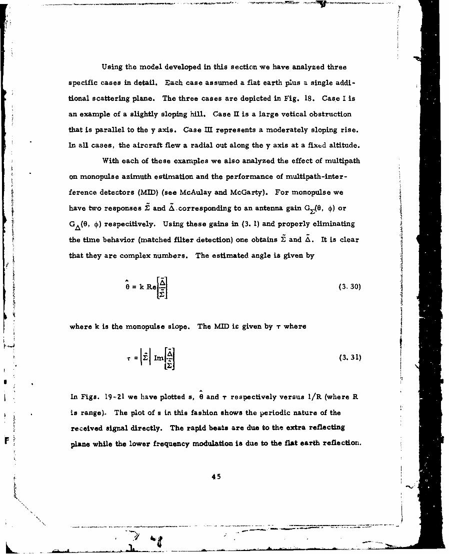
Using the model developed in this section we have analyzed three
specific cases in detail. Each case assumed a flat earth plus a single addi-
tional scattering plane. The three cases are depicted in Fig. 18. Cas.e I is
an example of a slightly sloping hill. Case II is a large vetical obstruction
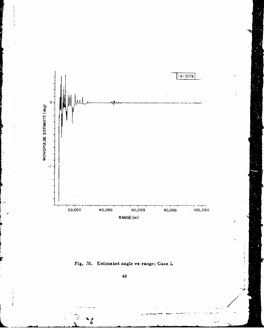
that is parallel to the y axis. Case Ill represents a moderately sloping rise.
In all cases, the aircraft flew a radial out along the y axis at a fixtd altitude.
With each of these examples we also analyzed the effect of multipath
on monopulse azimuth estimation and the performance of multipath-inter-
ference detectors (MID) (see McAulay and McGarty). For monopulse we
have two responses E and , .corresponding to an antenna gain G,(O, 4,) or
GA(O, 4) respecitively. Using these gains in (3. 1) and properly eliminating
the time behavior (matched filter detection) one obtains Z and A. It is clear
that they are complex numbers. The estimated angle is given by
= k Re[• (3, 30)
where k is the monopulse slope. The MID ic given by T where
i~mi (3.31)
In Figs. 19-Z1 we have plotted s, 0 and T respectively versus I/R (where R
is range), The plot of s in this fashion shows the periodic nature of the
received signal directly. The rapid beats are due to the extra reflecting
F'plane while the lower frequency modulation is due to the flat earth reflection.
45
a |
S-. -- -- "I-- -ll- -• \ ' I li
S.. . . . . . . . . . . . . .- .. . .. . . .

7~5 776
(b)
CASE IT a 0* Rz900xo=-20 , ymya1 OzOmzon0
(C)
CASE ::av40. 15;XOuO, Yea I0O,000m, ZO'0
Fig. 18. Geometry of reflecting plane for cases discussed.
46
4w1*_

j 1-4-157771
ii
0 1.-- V
0
Lu it LI
-1-- --
I I
0.000O. 0.00004 0.00000 0.00001 0.000010
l/Rim-1)
Fig. 19. Beam power ve inverse range; Case L
4"7
rI' !•(~ .I ,....,,!.
0-
I -
-J
0.
0
zi
oi
,' t T , ,--, 1 -r--r---T -r Ti-
20,000 40,000 60,000 80,000 100,000
RANGE (W)
Fig. 20. Estimated angle vs range; Case L
48
I ,.,,/"
S• 1 ii I
S9 I

0.002
Q
:, • I jDETECTION THRESHOLDC-)
}.-
Cn
2I
-0.002
-0.004 T______ __ __ __ __-r-__ __ _
o20,000 40,000 60,000 eo,0oo 100,000RANGE (m)
Fig. 21. Multipath test vs range; Case I.
49e ,
J.•..
'~~~ "WNdl •
The angle estimate in Fig. 20 for Case I shows the combination of both fading,
SNR losses, and the multipath bias modulation effect note by McAulay and
McGarty. The plot of T shows how such multipath is registered by this detec-
tor by its passage beyond the detection thresholds shown. These cases were
done for 512 element dipole array that was tilted down 40 and had a 3 dB/degree
vertical cutoff below the "horizon."
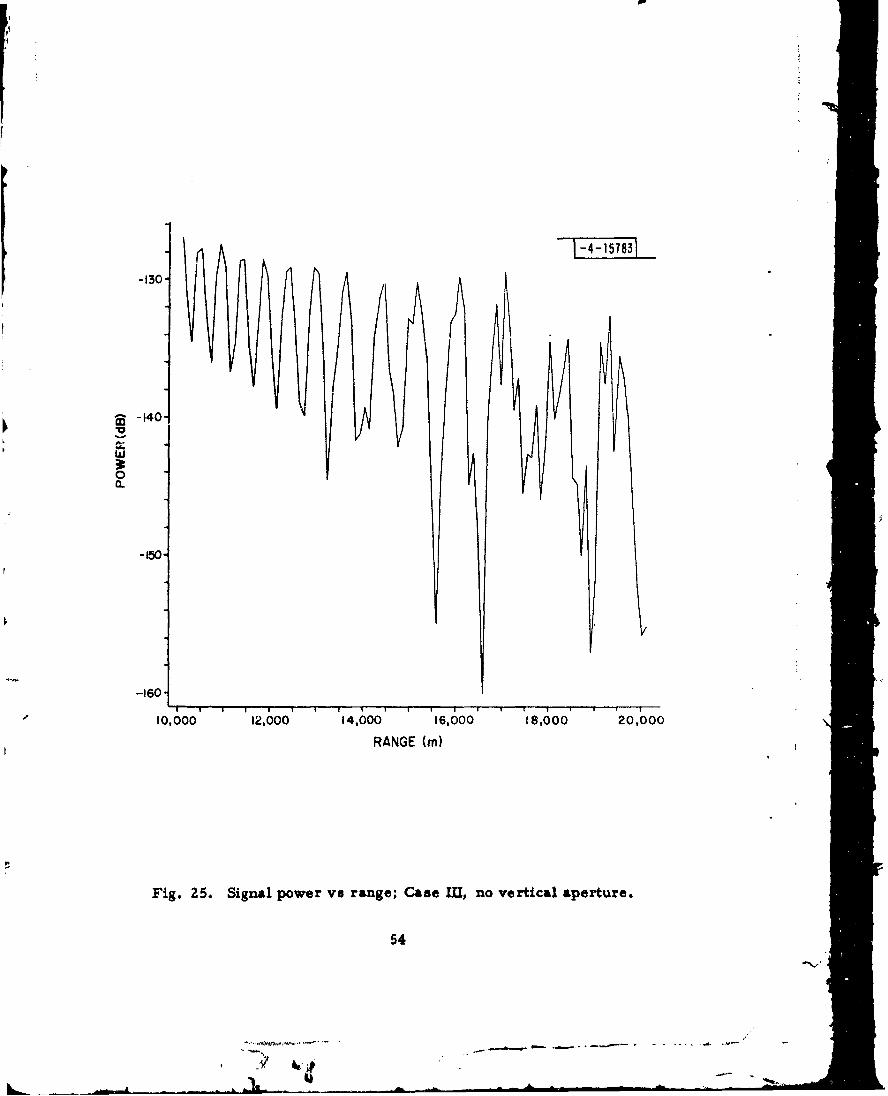
In a similar fashion, Case II is shown in Figs. 22-24. Here the mul-
tipath effect on angle estimates is more clearly pronounced in Fig. 23. Case
IMl results are shown in Figs. 25-27 Lor a hogtrough antenna and in Figs. 28-
30 for an antenna with vertical aperture. What is most clear here is that
vertical aperture does help significantly in reducing the angle errors (Fig. 29).
This is a result of increasing the effective SNR as is evidenced by comparing
Figs. 25 and 28.
Various other analyses are possible that exhibit the effects of in-
creased surface roughness, changes in the electrical properties and other
reflecting plane orientations.
3.4 CONCLUSIONS
The effects of reflections from large smooth surfaces has been
modeled as the coherent sum of plane waves incident on the antenna aperture.
The waves can be completely characterized by their ampli Je, phase,
azimuth and elevation relative to the boresight of the antenna. In Zhis section
we presented a detailed model which could be used to develop a received sig-
nal which would be representative of specular multipath.
The specular multipath model developed depended upon the following
points:
50

4/
[-4 -157o-120 ]
- I'-140
II
hD• -150
-160I
-170
- 180
10,000 12,000 14,000 16,000 18,000 20,000
RANGEWm)
I
Fig. 22. Beam power in dB vs range; Case II.
51 •
-- i i
,/' 4.~l

2-
0-
wS-2-
ww-j -4-
a.l
0
0
;0,000 12,000 14,000 16ý00 18,000 20,000
RANGE (in
Fig. 23. Monopulse azimuth estimate; Case II.
52
/m
- - . .. .

0.001
I--
I.-
I //
4 0
-0.001
I 1 " I ' ' "
10,000 12,000 14,000 16,000 18,000 20,000RANGE (m)
Fig. Z4. Multipath detector output; Case IL
53
.1 ~ -
a.
-130.
-160-
10,000 12,000 14,000 16,000 18,000 20,000
RANGE (in)
Fig. 25. Signal power ve range; Case LU, no vertical aperture.
54
- .-. -....

SI-4-15 7841
0.50 A
Ri
U,W ow
0~z0
-0.50.
10,000 12,000 14,000 I6000 18,000 20,000RANGEWm)
Fig. 26. Monopulse azimuth estimate; Case Ml, no vertical aperture.
55- ---. me -
I 3!
0.0006.
0.0004-
0n 0
I-0.0002.
F:J
D
o-oo-0004-!s8s
S.
I.-
-. -0,0002
- 0.0004 ••
-0.0006 ,
-0*0008 .....10,000 12,000 14,0C0 16,000 18,000 20,000
RANGE(m)
Fig. 27. Multipath detector statistic; Case IL no vertical aperture.
56
/
".~__.-=

7i1-15861
J
-90,
10,000 12,000 14,000 16,000 18,000 20,000
RANGE (i
ii
Fig. 28. Signal amplitude vs range; Caae LUI, vertical aperture.
57
W */ b

0.3
0.2
- 0.1
ww(In 0a-0z0
-0.I
-0.2-
10,000 12,000 14,000 16,000 18,000 20,000
RANGE(m)
Fig. 29. Monopulse axim~uth estimate; Case flI, vertical aperture.
58
- 4w - .--

I.|
0.002-
SI-i
III
I---~s
- i
S-0.001.m
0e
-0.001.
-0.002-
-0003
10,00 12,000 14,000 16P000 18,000 20,000
RANGE(m)
IIi
Fig. 30. Multipath detector; Case UL vertical aperture.
59L- ii - I
!= _... _.

p•
Geometry: For each multipath source a plane was posi-
tioned at the source location and tilted in both range and
cross range directions to coincide with the actual surface.
Evaluation of propagation distances could then be made
directly knowing the location of the receiver and trans -
mitter. All geometrical constants were determined for
each multipath reflector in terms of the offset position of
the plane, its range and cross range tilts and the locations
of transmitter and receiver.
2. Reflection Coefficient: The effect of a multipath signal on
azimuth estimation and link reliability depends directly
upon how Strong it is relative to the free space signal.
The ratio of multipath to free space signal amplitudes is
given by the reflection coefficient. These were
a. Electromagnetic Reflection: This is determined
by the Fresnel reflection equation for a plane S
wave at the interface of two media with differ-
ent electrical properties.
b. Diffuse Multipath: This represents the fraction of
incident radiation that is not lost to other than the
specular direction as a result of surface roughness.
c. Diffraction: If the surface is of finite size than its
location and size must be ¢,nsidered. This results
in a study of where the scattering aperture falls
relative to the Fresnel zone projected on the scatter-
ing plane.
60j
"--- I 1 •
I)!
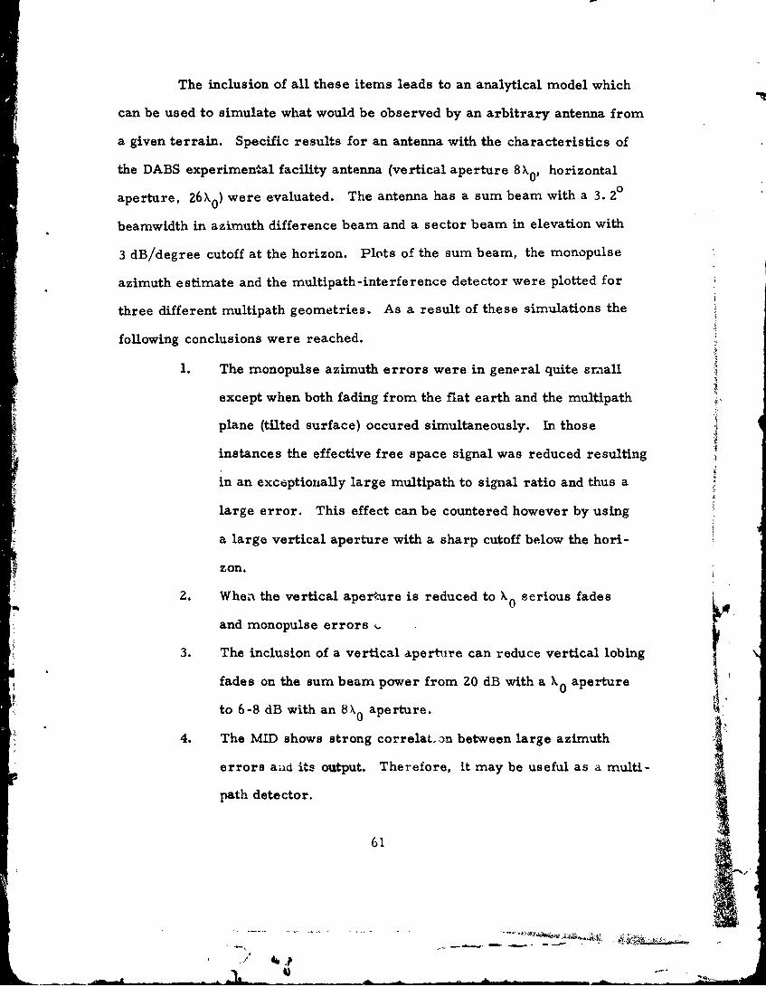
The inclusion of all these items leads to an analytical model which
can be used to simulate what would be observed by an arbitrary antenna from
a given terrain. Specific results for an antenna with the characteristics of
the DABS experimental facility antenna (vertical aperture 8X0, horizontal
aperture, 26ko) were evaluated. The antenna has a sum beam with a 3. 20
beamwidth in azimuth difference beam and a sector beam in elevation with
3 dB/degree cutoff at the horizon. Plots of the sum beam, the monopulse
azimuth estimate and the multipath-interference detector were plotted for
three different multipath geometries. As a result of these simulations the
following conclusions were reached.
S1. The monopulse azimuth errors were in general quite sm~all
except when both fading from the flat earth and the multipath
plane (tilted surface) occured simultaneously. In those
instances the effective free space signal was reduced resulting
in an exceptionally large multipath to signal ratio and thus a
large error. This effect can be countered however by using
a large vertical aperture with a sharp cutoff below the hori-
zon.
2. When the vertical aperture is reduced to X serious fades0
and monopulse errors
3. The inclusion of a vertical aperture can reduce vertical lobing
fades on the sum beam power from 20 dB with a X,• aperture
to 6-8 dB with an 8k0 aperture.
4. The MID shows strong correlat.on between large azimuth
errors alci its output. Therefore, it may be useful as a multi-
path detector.
61
4b.'AI Il l
"!- A _____ "

The simulations discussed in this report represent only a small
number of those that have been performed. Furthermore, recent compari-
son!l of simulations with actual data obtained at DABSEF indicate that the
model does represent the observed phenonmena quite well in many cases.
62
-.- -~ . . .

SECTION FOUR
DIFFUSE MULTIPATH
Diffuse multipath is a random phenomenon, distinct from specular
multipath, and must be treated as such. In contrast to the development in
the last section, where exact descriptions of the scattering surface were
given, in this section the nature of the scattering surface is describable in
only a probabilistic sense. The reason for this is that the diffuse multipath
arises from the roughness of the surface and is predominantly a diffraction
effect. This will become important when we analyze the effects giving rise
to the scattered field.
In the estimation of the azimuth of a cooperative 3ignal source, the
effects of multipath tend to degrade the performance of such estimates. The
multipath encountered has been divided into two different categories, specular
Si diffuse. Specular multipath res'..lts from large smooth surfaces occupy-
ing a significant part of the first Fresnel zone. Diffuse multipath differs
from the specular form in that when it is scattered, it does not propagate in
a single direction but in a continuum of directions, depending on the rough-
ness properties of the scattering surface. Diffuse multipath is a diffraction
phenomenon where the element doing the diffracting is a small surface per-
tubation.
The effects of such scattering were discussed by Kerr(1951) in an
attempt to analyze the effect of sea surface scattering on radar performance.
63
The approach used by Kerr was to obtain a scattering cross section for the
surface. A more detailed approach was undertaken by Rice (1931) when he
modeled the surface by means of a deterministic polynomial atnd then solved
the random problem. His approach was quasi-deterministic and directed at
sea surface scattering. A different approach using the Yirchoff approxima-
tion was presented by Eckart (1953) and was directed at acoustic scattering
from rough surfaces. Equations for the field were obtained and then averaged.
The resulting equations were then solved for the required quantities. This
work was latter followed by Ament (1953, 1956), using a similar approach.
Hoffman (1955) extended the analyfAs to the vector problem encount-
ered in electromagnetic field problems, using "'e Kirchoff technique. Other
attempts were made by Clark and Herndry (1964) to evaluate backscattering
effects. The prime reference using the Kirchoff method is Beckmann and
Spizzichino (1963). Their results give the field decomposition in terms of
different scattered directions. They assume a Gaussian surface behavior
with knowledge of surface standard deviations and correlation lengths. Experi-
ments yielding these values have been discussed by Fung and Moore and Hayre
and Moore.
Most of these previous results are not suitable for an analysis of
azimuth estimator performance, however. It wa.s shown by McGarty (1974),
for the case of bearing estimation with a sonar array, that a function called
the channel spread function was necessary to evaluate performance. This
function gives the intensity of radiation incident at the receiver from all direc-
tions. This function cannot be obtained from the Beckmann. and Spizzichino
model. However, analyses by Kodis (1966) and Barrick (1968) provide exactly
64
'o '.
what is necessary for the performance determination. Their analyses obtain
a scattering cross section which relates the scattered radiation into a specific
direction from a specified incident direction. The method of analysis differs
greatly from others in that it solves the scattering problem first using a
stationary phase technique (similar to Twersky (1957)), and then an averaging
technique. The averaging technique yields a very physical formula for the
scattering cross-section. It is in terms of the average number of scatterers,
the average surface curvature (following Longuet-Higgins [1, 2]) and reflection
coefficient.
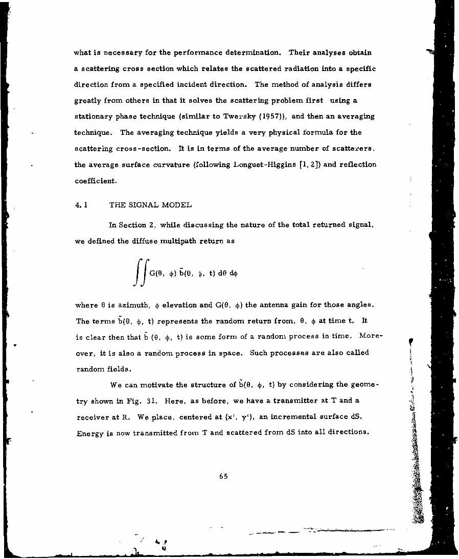
4. 1 THE SIGNAL MODEL
In Section 2, while discussing the nature of the total returned signal,
we defined the diffuse multipath return as
ffG(e, 4) b(O, 4, t) dO d--
where 0 is azimuth, ý elevation and G(O, p) the antenna gain for those angles.
The terms b(O, ý, t) represents the random return from, 0, 4 at time t. It
is clear then that b (0, 4, t) is some form of a random process in time. More-
over, it is also a random process in space. Such processes are also called
random fields.
We can motivate the structure of b(8, 4, t) by considering the geome-
try shown in Fig. 31. Here, as before, we have a transmitter at T and a
receiver at R. We place, centered at (xl, y'), an incremental surface dS.
Energy is now transmitted from T and scattered from dS into all directions.
65
-ad

Th~iisies
TdS
R
S
yi y
IHI
p.p
xi
Fig. 31. Diffuse multipath geometry.
66
- -.
S/ 'B,,

The amount arriving at R will depend on the diffraction nature of the surface
(recall our discussion in Section 3. 2. 3).
The azimuth 0 and elevation 4 are shown in Fig. 31. It will be shown
latter that each (x', y') pair uniquely corresponds to a (0, 4) pair, thus with
this one-to-one transformation we can equivalently phrase the multipath in
terms of these variables. Let us now also consider the temporal behavior
of b (0, 0, t). Since we are assuming that the surface is not moving and that
T is moving slowly compared to the measurements, the temporal behavior of
the received signal is merely that induced by f (t). Specifically, with these
assumptions we have
•(e, 4), t) c(e, 4) f(t - -) (4.1)
where R is the path length 'I'•. This then represents the effect at R at time
t of the source at T radiating onto dS. The term b(O, 4) represents the ran-
dom nature of the signal at R at time t.
Consider now some point r which lies in the receiving aperture
as shown in Fig. 32. Now the total reflecting surface can be viewed as the
source of many waves incident on r. Specifically, the surface dS generates
a wave incident from direction k as defined by the vector from r to dS. Thus,
we can consider each of the contributors from this surface to point r as the
contributor of a plane wave with an amplitude b(O, 4) or equivalently b(k)
where k is uniquely defined by 0 and 4. This allows us to write for an iso-
tropic (omnidirectional) receiver at r the observed signal as
I |_ _ __

S~T
dS.
Fig. 3Z. Geometry of receiving aperture.
68
/"
i H
s(r, t)(t exp(j k .r)fi(t -~dk .(4.2)
For simplicity, let us assume that the variation of f(t) is small so it can be
neglected. Thus we consider 8(r) where
s(r) = g•_) exp(j k r) (4.3)
Here b(k) equals b(O, c) and k • r is merely the projection of the incident
direction vector on r.
We now define the properties b(k) should have to be consistent with
properties of s(r). Note that s(r) is a random field in r generated by b(k).
The first assumption on b(k) is that it is a zero mean Gaussian random field.
Thus
Efb()]= 0. (4.4)
This assumption is consistent with the roughness assumption leading to the
definition of diffuse multipath. Since it is Gaussian, all we need for a corn-
plete statistical description is the covariance. That is, we need
E[s(r) (r K (r, r') . (4.5)
"* This is written as;
K5 (r, ii = ffff ) ,*(k')] exp(j k r -j k'r')dkdk'
(4.6)
69 u
It is convenient at this point to assume that s(r) is a homogeneous
random field over the aperture so that;
Ks(r, r') K s(r-r') . (4.7)5- ii-
This implies (see Yaglom) that; =
.EýbQk) b (k')] = K(k) 6(k -k') (4.8)
where 6(k - k') is a two dimensional implse function. The function K(k) or
K(O, 4)) is called the channel spread function and it is a measure of the energy
coming from direction (0, 4) to the point r.
It is the channel spread function that defines the angle estimation per-
formance of antennas (see McGarty [1]) and thus plays a dominant role in deter-
mining the effects of random multipath phenomena. It is the evaluation of this
function from first principles and the use of it in system performance evalua-
tion which will interest us ir dis section.
4.2 THE CHANNEL SPREAD FUNCTION
To evaluate the effect of dcifuse radiation on azimuth estimation per-
formance, it is necessary therefore to determine the channel spread function.
To obtain this function, we must first evaluate the time behavior of the irra-
diated surface and also the radiation pattern of incremental portions j, the
surface. Once these two relationships are obtained, the spread function can
be obtained directly.
70
-- -. ----. ;
/
!' I

Consider a point source located at positon (0, r, z2 ) on the flat
earth model as shown in Fig. 33. A receiver is located at (0, 0, z 1 ). The
source emits a spherical wave which begins at time t 0 and is received by the
receiver at time t 1 where
tc t + 0 (4.9)
where d0 is the distance between the source and the receiver and is given by;
d r 0) . (4.-10)
The power density of the wave received at the receiver is P/(4 2) where Pe
is the power of the source.
The source also irradiates a portion of the surface of the earth and
this surface scatters the radiation in all directions. The fraction of the inci-
dent power scattered to the receiver from the ith incremental area is given
by ait the scattering cross-section per unit area. Assume that there are N
such areas. Then, the total amount of power per square meter received at
the receiver due to the N discrete incoherently radiating surface areas is,
SN. where;N A
N T PO Ai -
i ( 1
I
71

118 -4_- 157
DIRECT PATH )--"-
z y
KY
Fig. 33. Geometry of direct path.
72
S~/
J1
where Ai is •ie area of the ith scattering section, RiH is the distance from the
receiver to the ith scatterer, and Rai is the distance from the transmitter to
the ith area.
Now, at any one instant of time, not all of the ground is illuminated
by the source. For example, at t = to the wave has just begun to propagate.
The minimum amount of time it takes for a wave to propagate from the source
to the receiver via a reflection from the earth's surface is,
r 2 +(zI +z 2 ) 2
ts c (4.12)
where c is the speed of propagation. At this instant, the area of the scatter-
ing plane illuminating the receiver is only a point. For t > t., we can find
the area by finding the equations of all (x, y) such that the distance R + R2
equals ct. The resulting area is that area from which the receiver obtains
power at time t. This follows directly from the fact that 11 is the distance
from the scattering point to the receiver and R 2 the distance from the scatter-
ing point to the source.
From the geometry of Fig. 34, it is clear that (
R 2 x 2 + yZ 2 (4. 13)11
and
22 2 24R 22x + (r -y) + z 2 . 4.14)
73

t..2
ILLUMINATED AREA
Fig. 34. Tixne variation of area.
74
..

Then, if we define for each time, t, a distance p as;
p = ct (4. 15,
we can show that the area irradiated which gives rise to signals received at
the receiver at time t > ts is bounded by the ellipse given by (see Appendix I)
a(y - yo)2 + b 2 x2 = ro 4. 16)
where
aZ= r(pz - r ) (4. 17)
b2 = 4p2 (4. 18)
_ (P2 r r2 + z 2ZZ)r
YO - 1 _ (4 19)
2(p -r)
and
z - 2 1(P z -+ z 2 )a 4z2(p - rz) (4. )ro=P . .. (pZ - r z4 o
Thus, for any time t, the surface from which radiation is received is bounded
by the ellipse given by (4. 16). We shall call the area of the elliptical surface
A(t). It is easily shown that as t -• •. the elipse turns into a circular region.
751 I"sI

Now, if we assume that the receiver is omnidirectional, then we can
calculate the total power density at the receiver. This can be obtained directly
from (4. 11) as a limiting case. Namely, if a-(x, y) is the fraction of incident
power scattered from (x, y) into the receiver, then the total power density at
the receiver at time t is given by S(t) where
S(t) 0 cr(x, y) ix dy (4.21)
A(t) 1 2
where A(t) is the bounding ellipsoid.
There is an important interpretation of Eq. (4. 21) worth noting. Con-
sider the special case of a reflector which scatters the incident radiation uni-
formly in all directions. For this case we let a-(x, y) equal a0 and obtain for
S(t);
rPO
S(t) - 0- dx (4. 622)
(4 t) A It
S(t), now in Eq. (4. 22), is the power per square meter at the receiver at time
t. As t increases, the ellipse grows; however, the Lwerse ai- tance squared
values weight contributions less and less. It can be shown that (4. 22) approaches
a limiting value at t - -o. An exact calculation is shown in Fig. 35. Here,
we have plotted S(t) versus time for r = 15 ,m, z1 = 10 m and z2= 3km.
Note :.,w rapidly S(t) approaches almosL a sf.; ady-state value. What this
76
- |!

r--
3-
Eii
cr
O- L-4 -157930b
0.000050 0.000052 0.000054 0.000056 0.000058 0.000060
TIME (sec)
Fig. 35. Area, S(t), vs time (z1 = 10 M, z= 3 km, R 15 kmn).
77
A 1•

implies is that there will be little time fluctuation in the diffuse field due to
this effect.
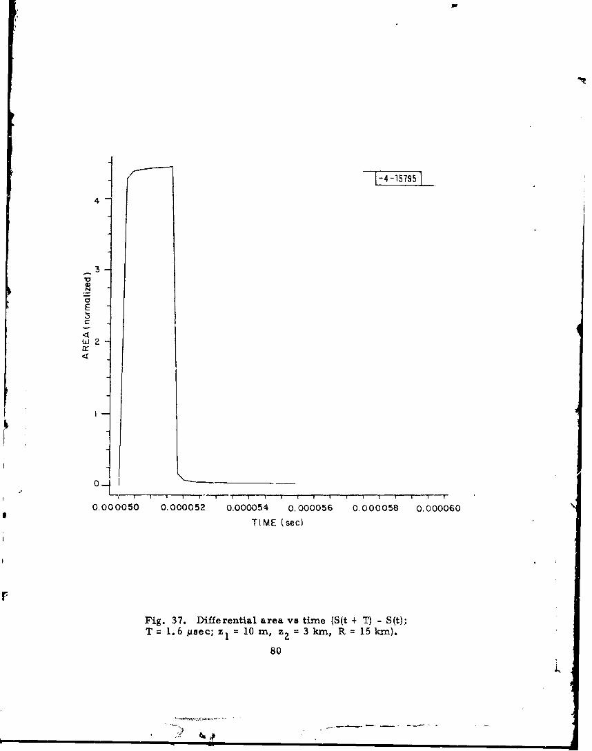
The response S(t) due to pulses is shown in Figs. 36 and 37. Here,
the source er.iits a I pLsec and 1. 6 ýtaec pulse respectively. The correspond-
ing power density is plotted. Again, note the sharp rise and cutoff values for
the diffuse radiation. The rise time is about 0. 5 Iisec while the decay time is
about 0. 25 pLsec.
To complete the analysis, the scattering cross section p-r unit area
o-(x, y) must be determined. To do this, we shall follow Kodis and Barrick
and obtain the function r(OS9, ýs ; 4). This is the fraction of the incident power
incident on a surface S from and angle Pi and scattered into direction (0s , 4s).
These directions are shown in Fig. 38. Here, it is assumed that the incident
field is a plane wave, making an angle ýi with the z axis and having a wave
vector lying in the y-z plane.
To obtain this function, we write the scattered field as
Esc(r) = - j '(r, rt) J(rl) dS (4. 23)
where r(r, r') is the dyadic Green's function given by (see Silver, p. 132)
P(r, r')= + 1 V (exp[j kr_ r' ]/(4Tr r - r_)) (4. 24)V k 1
and J(rl) is the surface current density c-nd j is 41J.
78
4"

S[-4 -1 i94]
4-
3m
a-,
V
E0
< 2-
0
0.000050 0.000052 0.000054 0.000056 0.300058 6.000060
SI
TIME (sec)
Fig. 36. Differential area vs time (S(t + T) -St)T I 1 Msec; z 10 in, z, 3 kmn, R 15 km).
79 *
[ --'Pu
4
3
E
0
N
t±2
S I . . . I ' • I I I I i ' i ' I ' I ' ' i . ... 1 ' '
0.000050 0.000052 0.000054 0,000056 0.000058 0.000060
TIME (sec)
Fig. 37. Differential area vs time (S(t + T) - S(t);
T 1.6 psec; = 10 M, z= 3kkm, R = 15 kin).
80

Th8-f-5 1961, -iJZINCIDENT WAVE
OinOs SCATTERED WAVE
INCIDENT PLANE OR
x
Fig. 38. Scattering geometry.
81

Using the Kirchoff approximation, Kodis shows that the field scattered
in direction k due to a source from k. is given by
E (kk)=2jk eJkr FE~sc(k.r 2jk) e j dS'(I_ - -sk k )(h_ x _i)
exp[j(k. - k) • r' (4. 25)
where
hk x e (4. 26)
and hiis the unit normal directed into the scattering plane at every point and
t is the polarization vector of the incident field. Using the method of station-
ary phase and then averaging, Kodis shows that the scattering cross section
is given by
0-(Os 4s; d) = lTnA< I l r.1>tR(ý)I2 (4. 27)
i
where nA is the average number of specular points per unit area,< Ir r21 >
the average absolute value of product of principal radii of curvature, and R(ý)
the reflectioi. coefficient. The angle ý is the local angle of incidence at the
specular point and is given by the relationship;
cost = J• sin 4 sin cos 01 + cos 4i cos (* (4. 28)
82
I, 4 •,,p

Barrick has shown that
n 7.255 exp tn-(4.29)wr 2- [(r
with
2
s 24 h(4.30)
where T- is the correlation length of the surface and ahis the variance of the
J ,h
surface height. tan y is given byI
tan y = Jsin2~ 2 siný sinc cs SO s 4 sin 24ý 4 'cos~ip+ cosý
The curvature has also been shown by Barrick to be
2
T i4
< r 1 r2 1 0. 1387 ir -4sec4 (4. 32)s
Finally, for vertical polarization over a perfectly conducting pl~ane, we have
for the reflection coefficient
2-Sin~ siný sin 0 +ia aa() s Z 3 (4.33)
83
--------

where
a 2 = cos4i sines + sinpi cosos coss , (4. 34)
a 3 = sinoi cosos + cosoi sinos cosOs (4. 35)
If we define a constant C as the product of 0. 1378 and 7. 255 then we
can combine (4. 28) - (4. 35) to yield;
cr(O~ S, 0; Oi) = Csc exp [-4 R(ý)j2 .(4.36)
This is the resulting scattering cross-section. We can observe its behavior
easily in this form. By using (4. 31) we first see that for positive Oi and 0.,
tan y increases as the azimuth s increases or decreases from zero. This
implies that tne angle y is increasing as an absolute value of the azimuth.
Thus for fixed 0, and Os the azimuth behavior of the scattering cross -section
is dominated by y which in turn is reflected in the two terms; exp(-tan2 y/s 2)
and sec y. The former term decreases with increasing y, the rate of increase
depending on the value of s 2. The latter term, increases with sec 4y, inde -
2pendent of s . Now two distinct regions are possible. The first is for large
s: In that case, the sec4 y behavior dominates a scattering cross-section
which increases with azimuth. Large s implies that oi,, the correlation
length, is small compared to the surface roughness. This can be calied a
very rough surface. For example, if ah is 10 m, then the value of cr needed
84
, i= i
'-SA _

to insure this condition is on the order of 10 m. A second effect to note is2
that the amplitude about zero azimuth depends inversely on s . Thus, a very
rcugh surface scatters less in the forward direction. The second region is
that in which s2 is small, i.e. , o >> a'h so that exp(-tan 2 Y/s 2 ) dominates
the profile of the scattering cross-section. Figs. 39-42 depict results for
varying cases. Note that in Fig. 40 we have almost a specular scatter sur-
face with minimum spread. This results from a very large value of a-P the
surface correlation length.
The assumptions that must be made concerning the surface in order
that the analysis leading to (4. 34) be consistent are (see Barrick):
1. The radius of curvature, p, everywhere on the reflecting
surface be much greater than the wavelength. Thus p >> » 0'
2. Multiple scattering effects can be neglected.
S... The mean square surface height is much greater than a
wavelength, that is a-2 Cos2 p >> X0*2
Condition (1) and (3) are direct limitations on the types of surfaces.
Specifically, (1) requires that the surfaces be very rounded since X 0 at 1090
MIhz is about one foot. Furthermore, (3) states that unless h is very large,
the approximations breakdown at grazing angles; 4 i -r r/2. That is most sur-
faces "look" like specular reflectors at grazing angles such that ýi - •/2.
Further limitations concerning the surface correlation coefficient
are discussed in Barrick (2]. He notes that the correlation must be quadratic
about the origin. Specifically, the result in (4. 36) assumes that the surface
height z is a Gaussian random variable with a correlation, E[z(x, y) z(x', y,)],
85

16
14-
12-
Z0
wW a
V)0
2-
0ý 7-rT7- _-
'II-10 , -6 -4 - 2 4 6 8 10
AZMUTH, ( (deg)
0IFig. 39. Scattering cross-section ve azimuth (0 = 88° = /), 8
86
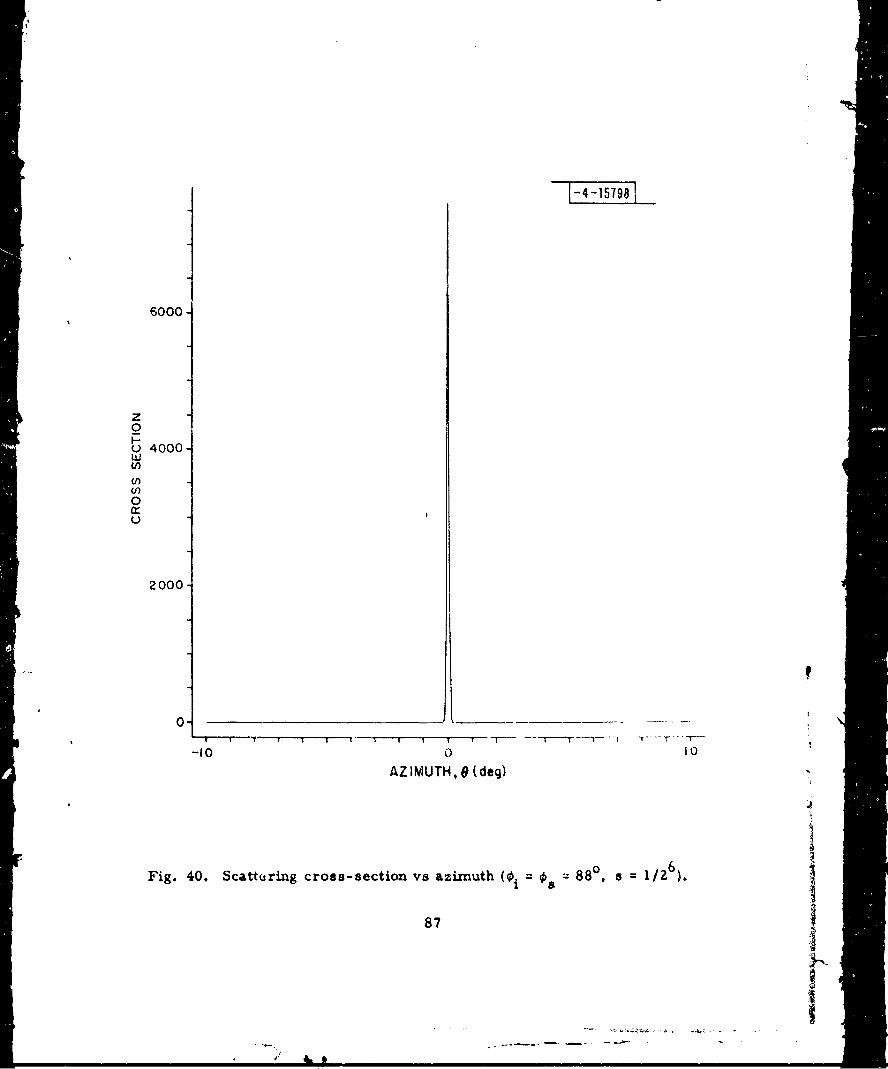
7 , •798L
6000
Z0F--U 4000wU,
0
2 000
0
, ~ T iir Iiir m
-I00 10
AZIMUTH, & (deg)
Fig. 40. Scattering cross-section vs azimuth ($ = 88° a = 1/26).
87 4

-4-15799E
4
z
0
0uJ
c•2
0/
-10 0 tO
AZIMUTH, 0 (deg)
Pig. 41. Scattering cross-section vs azimuth (i = 880, 0 = 2).
88
"•': " ' - -! - -al- -

0.02
z0I--
w
o 0.010
0-0
T 1 I t I I T F
-10 0 10AZMUTH, 0 (deg)
0 6Fig. 42. Scattering cross-section vs azimuth (& = 88 2
89
I i • l.

having the form, exp(- ) psI, where ps is (x - x')2 + (y - y,) . Thia fornn
ensures power conservation and correzt behavior as the ray optics limit is
approached.
4L We now want to evaluate the spread function K(O, *) which represents
the power per unit area per square radian incident at the receiver coming
from directions ý in elevation and 0 in azimuth. To do this, consider an incre-
mental area AS' as shown in Fig. 43. Draw a line from the origin at an angle
0 in the x, y plane, bounding dS' on one side and a line at angle 0 + AG bound-
ing AS' on the other side. Now 4 is given by
Stan- I T- ._ +(4.37)
The loci of constant s for constant z, are circles in the x, y plane.
Circles for ý and o + Aý are shown also in Fig. 43. The cross hatched area
in this figure represents the region of the scattering plane from which the source
receives radiation coming from the aolid angle •, 4 + A, and 0, 0 + AS.
The power per unit area received from this area is K(O, A) A0 61. Also,
AS is directly defined by the bounding region.
For any point in the area from Fig. 44, we see that
t - .z + .2 (4. 38)
The scattered angle ýs is given by (4. 37). The angle 0, the angle used for
the scattering cross-section is given by
90
,/

-- - ----
-
18-4-158o4]
IIFig. 43. Spread function geometry.
91
u - - . . . . . . . . . . .. m L

0' 0+ (4.39)
where
iItan- x~y (4.40)
Thus, we have for any 0, 4 pair
-P 4(e + , )dx dy-
SK(0, ,)-lim JI 1 ' (4.41)
-* 0
whereeis the intersection of the region formed as in Fig. 43 and the area of
illumination at time t. Note that x, y and 4). are functions of 6 and • so that
by using the Jacobian of the transformation some simplification of (4.41) may
result. However, another simplifying tool can be used if we introduce variable
PO where
-2O x +y , (4.42)
But, from (4. 37) and Fig. 44 we note that
PO zl tan 4 (4.43)
92
S~/

z
, t NORMAL TO
IX-Y PLANE
II
~(0, r, z2) :
Fig. 44. Scattering geometry.
93
Fig. 44 catrnggomty

Here pO is the radius of a circular coordinate system in the x, y plane. Then
x = PO sine = z, tan4 sinO (4.44)
y= pocosOeztan cosI . (4.45)
With these substitutions we can write ?P as in (4. 40);
-i a [ z, tan4o sinO (446r0, = tan-I [- z tan• cosJ (4.s46)
and
R = z1(1 + tan2) (4.47)
2 2 2 2R 2 = zi tan4 +r - 2r z, tan• cosO +z . (4. 48)
Then using the transformation from x, y into po0 0 the integral in (4. 41) can
be written using
dx dy pO dpo dO (4.49)
as;
94
.............
V/

K(O )o ffo-(1 +,(O, 4), ); ÷i(O,,))po dpo dO - (450)A0-~ 0 T(w)Z AS, R1 (O, 4)R72(914)
Kl, ) = lra(4.50 m
where we have assumed that A(t) is large enough (t >> to) and have explicity
stated,0, R1 and R in terms of 0 and P. Now using (4.49) and (4. 43) we can
take the limit to yield;
P 0ojO + 4(G, 4),4)i)(G, z 2 sec tan4
(41,) R ( ), R ((0,1'' 2
as the resulting channel spread function for this diffuse multipath field.
An evaluation of the channel spread function has been performed and
the results are shown iLz Figs. 45 to 48. This is for a time large enough so
that all the surface is irradiated. The ground antenna is assumed to be at
20 m and the aircraft at 1 km. The value of s varies as does the range of the
aircraft. In these figures, we have normlized (4. 51) by Po/4,wd and have
plotted 10 log1 0 of that ratio.
In Fig. 45, we have a fairly smooth surface (s = 0. 5). We note the
bright spot near the horizon and a rapid decrease as 0 goes from broadside.
A similar plot is shown in YF'. !A I-vt now the aircraft has quintupled its
range. We note the narrowing of the peaks. This narrow area is the glisten-
ing surface mentioned in Beckmann and Spichizzino. The remaining two plots
95

0.20
"1-1
0)0
-15d4 0.. r. *
-20 -to 0 -0-20
9(deg)
Fig. 45. Contour plot of scattering cross-section (R =10 kin,0 1 km, s 0. 5).
96
- -- 1 ---.--
I -' "/" ' ' '2C

1.1
-110800
-1~-15
404
-20 ~ -to 0 .02
(deg) - - .-
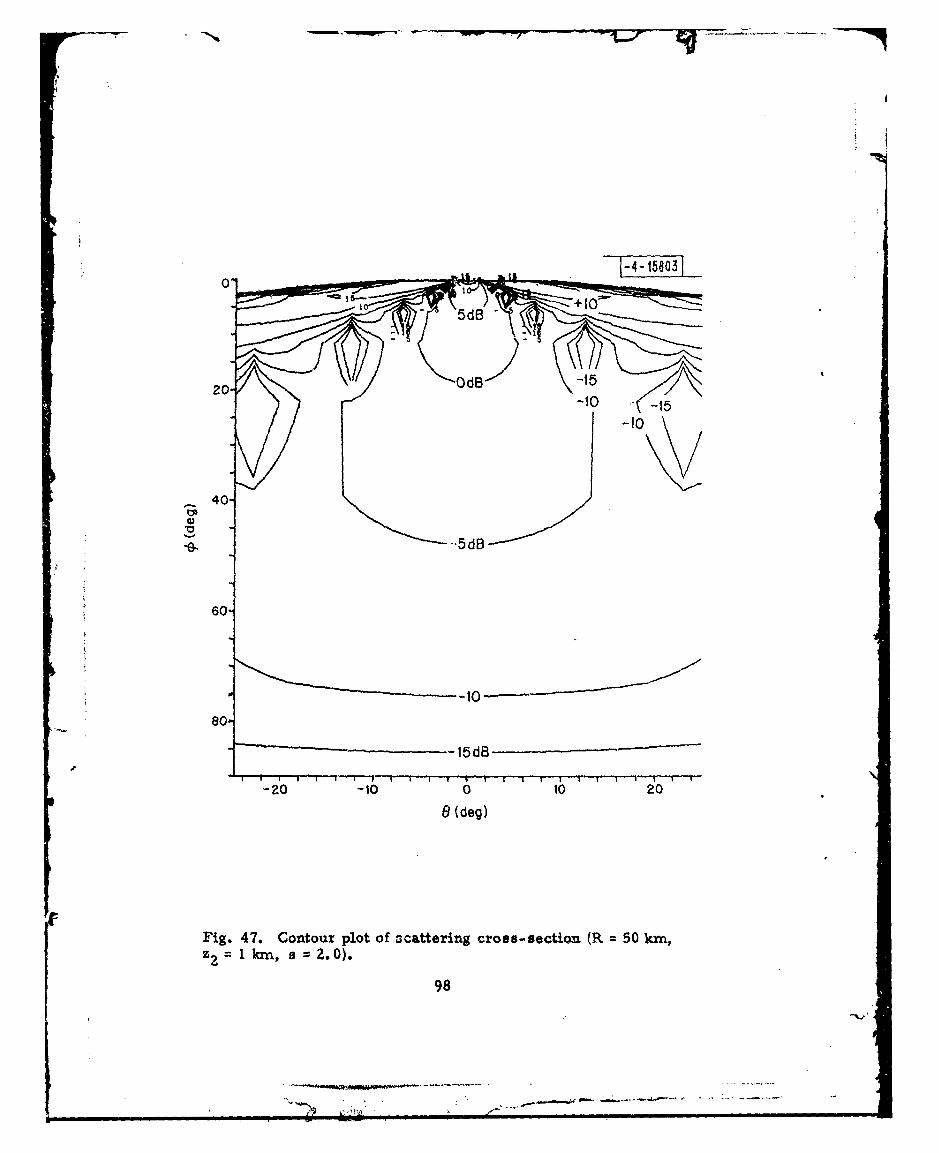
-10 -15-10
4 -,5dB
--------- 10 - -
80-
- ~~~~15d B-----
&(deg)
Fig. 47. Contour plot of ocattering cross-section (R =50 kmn,z I kmn, s 2. 0).
98
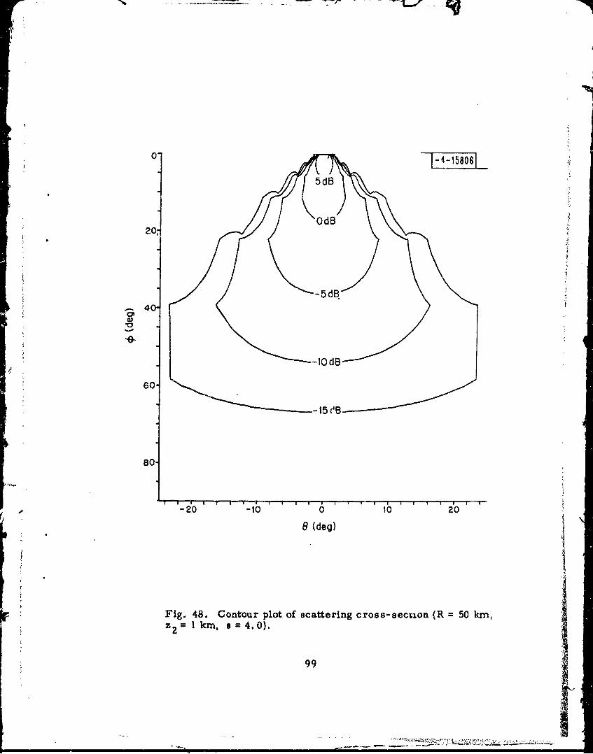
o' 1-4-158061
OdB
20,
-4dB-40
' -IOdB
60-
-15 eB
80
-20 -10 00 20 20
e (deg)
Fig. 48. Contour plot of scattering cross- section (R 50 km,z 1 krn, a 4.O0).
99 1
I ..

!EA
show how sidelobes appear as the surface becomes more rough. This is a
result of the increase in the radius of curvature term as well as a slow
decrease in the aver..ge number cf scatters as appear in (4. 51).
With K(8, %5), the aziimuth spread for a given antenna vertical gain
can be evaluated. Let G(%) be the vertical gain of the antenna; then, azim'zth
spread K(O) is given by
K(O) = G.) K(0, d) (4. 5Z)
As before, this is a function of 0 h' T z, r, and time. A sample plot
for r = 30 km using the vertical array proposed for the DABS antenna is
shown in Fig. 49. Note the sharp central peak and the drop of 6 orders of
magnitude as the azimuth increases. This profile is called the glistening
surface by Beckmann and Spizzichino.
It is also possible to use the gain in azimuth. Thus, if G(O, 4)) is tae
gain of an antenna in elevation and azimuth then, the quantity
_T
j j G(O, 4)) K(G, 4) dO d4,
= P (4.53)
7-77
100

100 R 20k "18-•-15,12]
Z2 2k
Z1 lOre
arh 1OM
101 T: 200m
200;
Z 20m
w0 -
w w2Z
I 10
-600
SAZIMUTH (deg)Al
; lFig. 49. Pl~ot of channel spread function vs azimuth for two correlation lengths.
101
SI.
I / I I.I
represents the diffuse energy-to-signal value for the given antenna gain
O(8, 4)). This has been evaluated in Fig. 50 versus range for the DABS
antenna. From this plot, we see that the dlffuse multipath is quite low and
would predict that it should not cause any difficulty in azimuth estimation.
4.3 PERFORMANCE
The azimuth estimation performance of an array is determined by
its beam pattern or ambiguity pattern, the inherent system noise, and also
the effect of multipath interference. For diffuse multipath, as the type dis-
cussed in Section 4. 2, the performance can be given in terms of the ambiguity
function and the azimuth spread function. We have the azimuth spread in
terms of
K(O) = j G(4) K(O, ,) d4 (4.54)
For the performance analysis we want K as a function of ý. which is cos8
where 0 = 900 represents broadside. Furthermore, we want K(p.) to have
unit area. Thus, we define the constant;
2' 2 K(O) dO (4.55)
as a normalization factor. Then, in terms of the function K(O), we have
102
/
4"• "" ------

T CORR LENGTH = 200m
Sh = lO re0-4 = 2km
ZI =lOri
0
1-
F-
-- . 20m
-_ _
0 20 40 60 so 100RANGE (km)
Fig. 50. Plot of multipath energy to signal vs range.
103
4,103

S(4)p z 1=cose . (4.56)
1
The ambiguit-. function of array is defined asI (p) and is given by
' (p.') jknlf) ';(4. + 'l2 (4. 57)
where !(4) is the N x 1 complex vector
[exp(-j zTdNlI/XO)
m . (. (4. 58)
~exp (-j2¶rd NI/X 0 )
Here, d is the displacement from the origin of the ith dipole receiver (for a
dipole array), k0 is the wavelength, and N is the number of dipoles.
The total eignal energy is given by
. = Gb E (4.59)
b2
where E is the energy of the transmitted pulse and ob represents channel
attenuation effects. The total diffuse multipath signal level is
S 2
c E s Uri (4. 60)
104
ig. , ' N'1

since we assume the signal due to diffuse multipath has been generated by
the source. The noise is assumed to be a zero mean Gaussian white noise
process, independent from element to element in the array and has a variance
given by
2- 0 (4. 61)n
For analytical purposes it becomes convenient to define two ratios, the multi-
path-to-signal ratio, •, and the noise-to-signal ratio, y. These are
2
(4.62)
V2
Y n (4. 63)S
Now i- has be en shcown elsewere that the Cramer-Rao bound for estimating R
is giv'er by (McGarty [1r);
' 1-var - •) - (4. 64)
where
105
A'. - .
0
+ 2-j K(,) 8(j -RI,) d (4.65)
where
N22 2+ 2
S-(4.66,N °'n (•n-+ 'T- NZ+s a-
4 =fK(4') 23(Fl - IV') dR, (4. 67)
By using (4. 63), we can rewrite (4. 66) as
C (N 2 + :•) (4.68)yN(Nz+ gO+ Ny)
and the term in the brackets in (4. 65) becomes
(+ K (R1) t- (R -) •d' (4.69)
The bound on or can be shown to relate to 2 as;
106

2 cot 0 2(o0 =-tan e+tan V + 0 s
where 0 is the pointing angle. Note that 0 = 90° impLes broadside.
Now the evaluation of (4. 65) can be facilitated by using Fourier trans-
form relationcliips. This has been discussed elsewhere but the evaluation of
the performance curves in Fig. 51 have been evaluated using this technique.
(See McGarty [1j.)
We can express the performance as a function of the beamwidth of
the array as follows. Recall that for a linear array, we have for the ambiguity
pattern
s(in [n-lT1 (4.71)
Sin fIý
where d equals Zird 0 /k 0 , d0 being the interdipole spacing and X0 the wavelength.
The first null in this pattern occurs at 'B where
Nd (4.72)
The center of the beam is at R = 0 so that the beamwidth between nulls
is given by
-1 0ýL in I0_ (4.73)
107
- -- - j-- q

mop - -
0.024
do= 0O. 15m0.02 -f = 1090mHz
S/N -400:sin-1 Xo
Nd0
0.016
.0IWITH DIFFUSE MULTIPATH
0.008WITHOUT DIFFUSE MULTIPATH
0.004-
I I I I i0 1 2 3 4 5 6
86 (deg)
Fig. 51. Standard deviation of angle estimate.
108
..... ..... ,..,,,, m*== •= . _.,_ ..... . .. -- - ._- -

From McGarty (1], we have the performance bound in the absence
of multipath which yields the standard deviation of the azimuth estimate, (r
in terrrms of the signal-to-noise ratio and the number of elements. It is
-0(radia 12 (4.74)

° 2 =o2 no multipath + fK(&) (t - p') dii) (4.77)
That is, the variance is increased by a factor which depends on the multi-
path to signal ratio, ý, and the nature of the spread channel, K(g).
Plotted in Fig. 51 is a- versus 0B1 the beamwidth in degrees for do
equal 0. 152 m, a frequency of 1090 MHz, a signal-to-noise ratio of 25 dB,
and the interference-to-signal ratio of -20 dB. We use the spread function
for z1 equal to 10 m, z2 equal to 2km, range equal to 20km. rh was 10 m,
and o7, 200 m (as shown in Fig. 49). Note the behavior of the variance. As
0B decreases, T decreases almost linearly. The bound actually is dominated
by S/N behavior and is only slightly affected by the diffuse multipath. This
implies that for an array, with an 8X 0 vertical aperture and a 26X0 horizontal
aperture diffuse multipath will not be a significant problem.
4.4 CONCLUSIONS
Diffuse multipath can be modelled as a random phenomenon which
results from the rough and random nature of the scattering surface. In this
section we consider the effects of such randomness in detail. We first reviewed
the rather large body of work that already exists on scattering from random
surfaces and discussed the shortcomings or usefulness of several of the models
that have been proposed.
110
. ..- _AL_. ."-

-7-"
A specific model for diffuse scattering was then proposed. First
an analysis oi the area irradiated as a function of time was performed. The
result of this analysis was that for psec type signals the effects of finite time
propagation could be neglec.ted. Then using the Kodis-Barrick model the scatter-
ing cross-section per unit area was obtaine,' for a Gaussian surface with a
Gaussian correlation function. The resulting scattering 7tross-section 0(0s,
• s; *i) was evaluated in terms of the mean squarf- surface height, Th' the
correlations length of the surface, , , and the gtometrical parameters of the
point of scattering.
It has been shown that to evaluate the effects of random signals coming
from a continuum of directions, as is the case for diffuse multipath, the channel
spread function, K(O. ý), must be obtained. This function represents the frac-
tion of diffuse energy received from a given azimuth, 0, and elevation, c.
Using the Kodis-Barrick scattering cross-section and the geometry of the ground-
to-air surveillance link the spread function was obtained.
This section concluded with an evaluation of the effects of diffuse multi-
path on azimuth estimation. Several different types of surfaces were considered
and a simplified closed form analytical result for azimuth .drrors was obtained.
As a result of this study the following specific conclusions were
reached.
1. The Kodis-Barrick model for diffuse scattering cross-sections
is most appropriate for performance evaluations.
2. Time dispersion effects are not important for MHz data rate
transmissions with respect to diffuse multipath effects.
Lli
L•[

3. The channel spread function for ah < aI shows a distinct
glistening surface effect that has been noted by other investi-
gators.
4. The errors on azimuth estimation due -o diffuse multipath are
negligible and orders of magnitude smaller than those observed
for specular multipath. Thus diffuse multipath presents no
serious limitations in direction finding capabilities in DABS.
5. The effects of earth curvature and shadowing can be included
but their net effect is of second order and discussed in the next
section.
lrn
1n
4W4

SECTION FIVE
OTHER EFFECTS
In the past two sections, we have discussed the effects of specular
and diffuse multipath and have presented models with which the effects of
these sources of interference on system performance could be determined.
In so doing, we neglected certain factors which in some circumstances can
"become important. It is the purpose of this section to discuss these factors
and place them in their proper perspective relative to the general model.
5. 1 REFRACTION
The model developed in this report for specular multipath considered
the scattering plane to be flat. However, the earth is not ýIat, it has curvature.
If we consider any scattering point x, y and let r2 be the distance from the
k transmitter to x, y and rI the distance from the receiver to that point, then
Beckmann and Spizzichino (pp. 222-224) show that we must reduce the reflec-
tion coefficient derived in Section 3 by a factor D where
D= I + (5.-1)Se(rl + r .1 sin Y -
I.
where R is the effective radius of the earth and y is (w/2) - where is as
In Section 4. Than. for r1 r 2 << Re, this is close to unity and it can be
r neglected. In our analysis, we had also included the atteneation of 1/rlri
which, combined with D, would imply for large Re that
113SJiB
7-fl ,
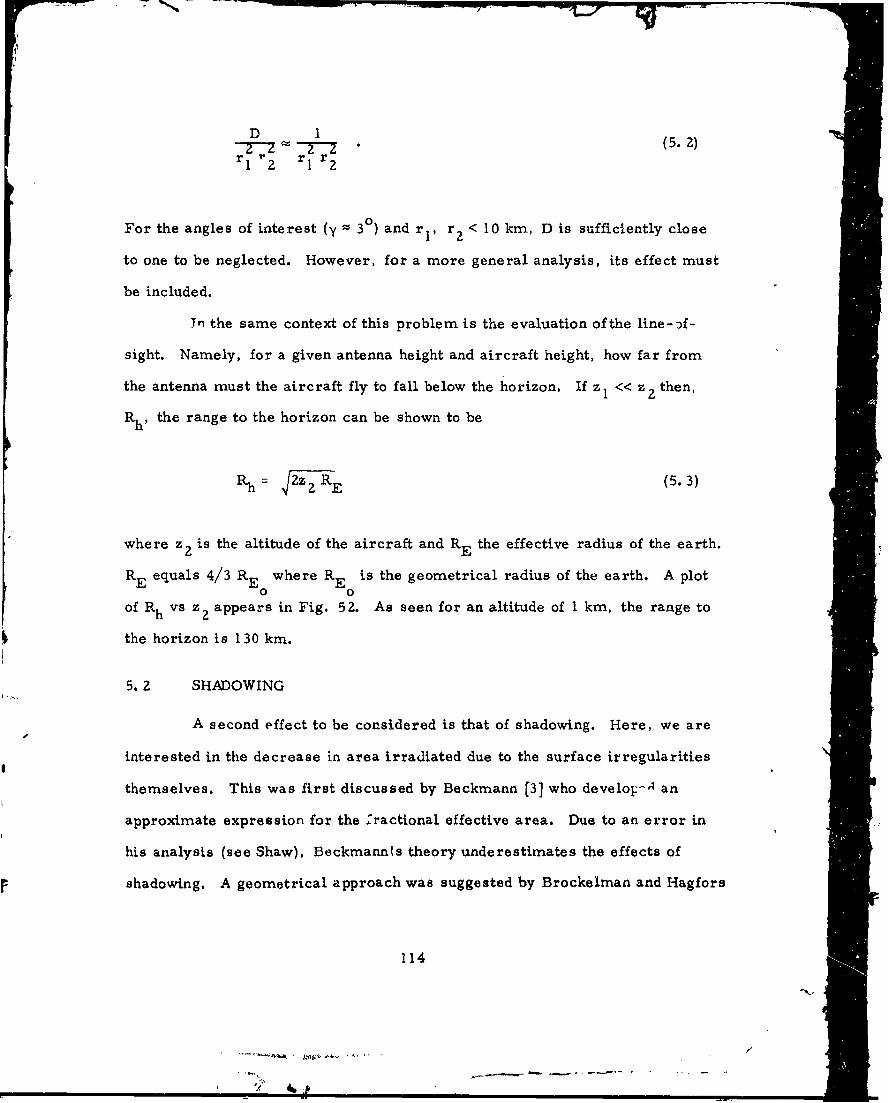
D 1 (5.2)
rl1r2 r r21ri
For the angles of interest (-y 30) and r 1 , r 2 < 10 kin, D is sufficiently close
to one to be neglected. However, for a more general analysis, its effect must
be included.
Tnr the same context of this problem is the evaluation of the line- -f- i
sight. Namely, for a given antenna height and aircraft height, how far from
the antenna must the aircraft fly to fall below the horizon. If z1 << z2 then,
Rh, the range to the horizon can be shown to be
Rh= ZZRE; (5.3)
where z2 is the altitude of the aircraft and RE the effective radius of the earth.
2P
RwE equals 4/3 RE where R Eis the geometrical radius of the earth. A plot
of Rh vs z2 appears in Fig. 52. As seen for an altitude of 1 kin, the range to
the horizon is 130 km.
5. 2 SHADOWING
A second effect to be considered is that of shadowing. Here, we are
interested in the decrease in area irradiated due to the surface irregularities
themselves. This was first discussed by Beckmann [3J who develoF=-- an
approximate expression for the 2'ractional effective area. Due to an error in
his analysis (see Shaw), Beckmannls theory underestimates the effects of
shadowing. A geometrical approach was suggested by Brockelman and Hagfors
114

10,00085 118 -4- -15815
1000-
b E
100(
10 I I ' . I _.! ,1 111 I I i1 12 4 6 810 20 40 6080100 200 400600 1000 2K 4K 6K 8K 1OK
ALTITUDE (m)
Fig. 52. Plot of aircraft altitude vs maximum range to horizon.
115
~4t ~1

and later by Smith. All of these analyses are predominantly for back scatter-
ing. A bistatic shadowing function was developed by Wagner. It represents
the effective fraction of the incident field scattered to the output direction. It
is given by
S(€, ¢)= [I - exp(- 2B1 + B 2)]
•(erf v 1 + erf v2)/4 (B 1 + B 2 ) (5.4)
where
I (ir/Z) - Pýi and
ý 2-(Tr/ 2) - ,with;
B. = [exp(-v ) - [iv. erfc v]/4 ov. (5. 5)
vi = I -lt/ (5.6)
T = tan cp. (5,7)
IPO = EiC(t) ý(t)] (5. 8)
O= i E [V(t) (t + T)i (5. 9)7 1 -r=O0
and ý(t) is the surface height (e. g., z(x, y)). Depending on the surface correla-
tion, (5.6) and (5.7) are directly evaluated. Wagner shows, that for the range
of values discussed in Sec-tion 4, S(•I, 4) is about 0. 1 This indicates an order
116
V

of magnitude decrease in the values of the field intensity evaluated there.
Since there appears to be little data to subtantiate these results, we did not
include them in the analysis.
5.3 SEA SURFACE SCATTERING
The scattering of electromagnetic waves from a sea surface is much
more complex than that from land. A great deal of both the theoretical
and experimental work has been done in this area but none as of yet directly
applicable to the DABS problem. The theoretical work by Beard [1]- [2],
Beard, et al., Bartick [1-[3] and the experimental work of Bass, et al., [1]-
[2) provide some insight into the problem. In particular, it has been noted
that specular type reflections can arise in other than the expected specular
direction. Furthermore, the difference between diffuse and specular reflec-
tions is not as clear as that developed in Sections 3 and 4.
The work by DeLorenzo and Cassedy has shown how one might analyze
and interpret the results. Their model assumes that the surface of the ocean S
is a narrowband zero mean Gaussian random process. They assume that the
height of the ocean, z(x, y), depends only on x and that (see Fig. 53) 1"
"4
E[z(x)Jz 0 (5.10)
4E[z(xl) z(x)]= K(x - x2 ) . (5.11)
The field, z(x), is homogeneous. A
117
'* ..
4 ',
,• ' • ... ...... ,•. :•,:,..•;:.: :•{

T118-4-158161
Fig. 53. Model of ocean wavesB.
118
t/.,
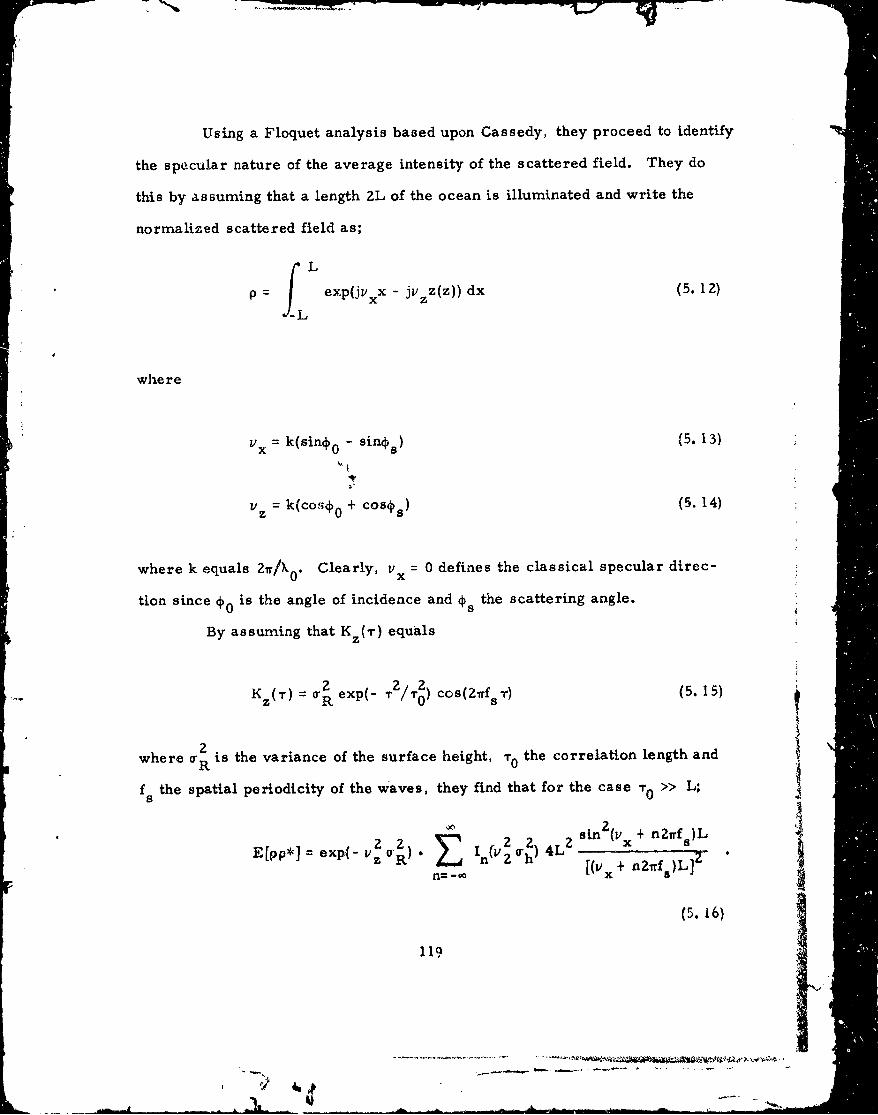
Using a Floquet analysis based upon Cassedy, they proceed to identify
the specular nature of the average intensity of the scattered field. They do
this by assuming that a length 2L of the ocean is illuminated and write the
normalized scattered field as;
p f exp(jvxX - jvzz(z)) dx (5.12)
whe re
Vx= k(sin - sins) (5. 13)
Vz = k(co,,• 0 + cos4s) (5.14)
where k equals 2rr/XO. Clearly, vx = 0 defines the classical specular direc-
tion since ýO is the angle of incidence and the scattering angle.
By assuming that K z(T) equals
2 Z2K () - exp(- TT cos(Zrf) (5. 1
where a2 is the variance of the surface height, T. the correlation length and
fs the spatial periodicity of the waves, they find that for the case T» >> L;
E[pp*] exp-) In(vP 'ovh) 4L' sin (v +n2 fa)L
z R n=-- 2 h [(vx + n Zrf )L]Z
(5.16)
119a

This expression shows the scattered power to be strongly peaked at
v + 2rnf =0 . (5.17)x 8
Obviously, vx = 0 is one of these values but so too are other directions.
DeLorenzo and and Cassedy show data which substantiates their model, Other
variations of the surface parameters introduce diffuse-like scattering along
with multiple specular scattering directions.
Thus, the analysis of the effects of multipath over the sea appears to
be quite complex and still an open area on many issues.
5.4 COMPOSITE SCATTERING
The fourth and final extension would be the scattering from composite
surfaces as discussed by Beckmann [1]. Basically, a composite rough surface
is one having several ah and oa-. Beckmann. shows that the total energy from
such a surface is the sum from all of its composites. To do this in practice
requires a better understanding of the surface topography. The studies by
Fung and Moore and Hayre and Moore do not seem to indicate however, that
such composite behavior is common.
"5.5 CONCLUSIONS
Those other effects that were not considered in the analysis of specular
and diffuse multipath in Sections 3 and 4 respectively represent only second
order perturbations on the results. The earths curvature giving rise to diver-
gence alters the result only slightly. The only serious limitation of having a
120

curved earth is that of line of sight limitations. These can be easily included
as a cutoff at maximum range.
The effects of shadowing are also only second order and only tend to
further reduce the effects of diffuse multipath. However, sea surface scatter-
ing does present a phenomenon for which little data in the L band regions exist.
This effect will undoubtedly be important at airports which are adjacent to the
ocean. To a first order the sea surface can be considered as a slightly rough
fiat plane with no tilts. This would indicate that azimuth errors would be small.
There are two other effects which may be dominant in certain locations
and for which at present little is known. They are;
1. Vegetation Effects: The effect of trees and other forms of
vegetation must be considered when evaluating the reflection
coefficient. However, trees at L band represent a random,
finite thickness, lossy, dielectric scatterer. At present no
adequate theory is available to analyze this effect. DABSEF
"data indicate that a reduction in reflection coefficient
results.
2. Low Angle Effects: When the aircraft is at very low eleva-
tion angles, theory for flat surfaces indicate that p approaches
unity and very deep nulls occur. However, actual topography
is not perfectly flat. There are many different, albeit large
in area, surfaces of various tilts. Thus as the elevation
angle gets smaller the Fresnel zone gets larger and encom-
passes many independently oriented surfaces. The coherent
sum of the plane waves from these surfaces tend to cancel and
IZ1

the resultant deep nulls do not appear. Again no adequate
theory exists to model this phenomenon nor are adequate
data available on large scale correlaticn effects.
r..m
F . m*

SECTION SIX
APPLICATIONS
The models that have been developed for both diffuse and specular
multipath are useful in evaluating many of the important aspects of DABS. In
this section we shall discuss five areas in which these analytical methods find
application and discuss how the results may be applied. These areas have in
common an interest in how the signal behaves as a function of sensor type,
sensor location and aircraft location. In general, the resulting analyses and
conclusions will be based solely upon the specular multipath model, for, as
we have shown in Section 4, diffuse multipath is a second order effect.
6.1 PERFORMANCE
There are two aspects of DABS performance that are impacted upon
by multipath. The first is the communication link performance. The link
performance depends upon SNR which in turn can be seriously degraded when-
ever the signal fades due to coherent multipath cancellation. The depths of
these fades can be evaluated for various terrain conditions and the link perfor-
mance obtained. In Section 3, we found that fading depended upon geometry,
surface roughness antenna gains and sensor and aircraft locations. In con-
trast to a simple flat earth, single plane model, the model developed In Sec-
tion 3 was based upon a more robust set of conditions. It allows fade calcu-
lations and performance predictions to be made from multiple reflecting
planes of finite size and varying surface interface properties.
123
'L f

The second performance issue is that of azimuth estimation perfor-
mance. As was shown in Section 3, the errors in monopulse azimuth estima-
tion are dependent upon two effects. The first was a pure SNR fade and the
second was a coherent cancelling by the off-azimuth multipath plane. Simi-
larly, ATCRBS angle estimating schemes have also been analyzed and similar
error behavior has been observed.
* 6.2 LOCALIZATION
Section 2 was basically an analytical approach to specular multipath
* in that, for a given geometric,' -onfiguration, the resulting output signal could
be formed. The inverse of this technique, going from an observed output to
a given geometry, is the synthesis portion of the analysis and has been termed
localization. That is, by observing the output of an antenna and knowing the
model it is possible to obtain the angles ai, 0 as well as the offset location of
the planes giving rise to that signal. In such a fashion we can localize the
source of each specular multipath signal and identify it in the terrain.
From Section 3 we know that the specular multipath signal power,
sampled in time and normalized by the intensity of the direct path, is given by
n n
=1 + P + Z pics(6Sii)i= 1 i= 1
n n
+ Z Pi Pj cos(0 1 - 0j) (6.1)
1=1 j=l
lilj
124
Q tn
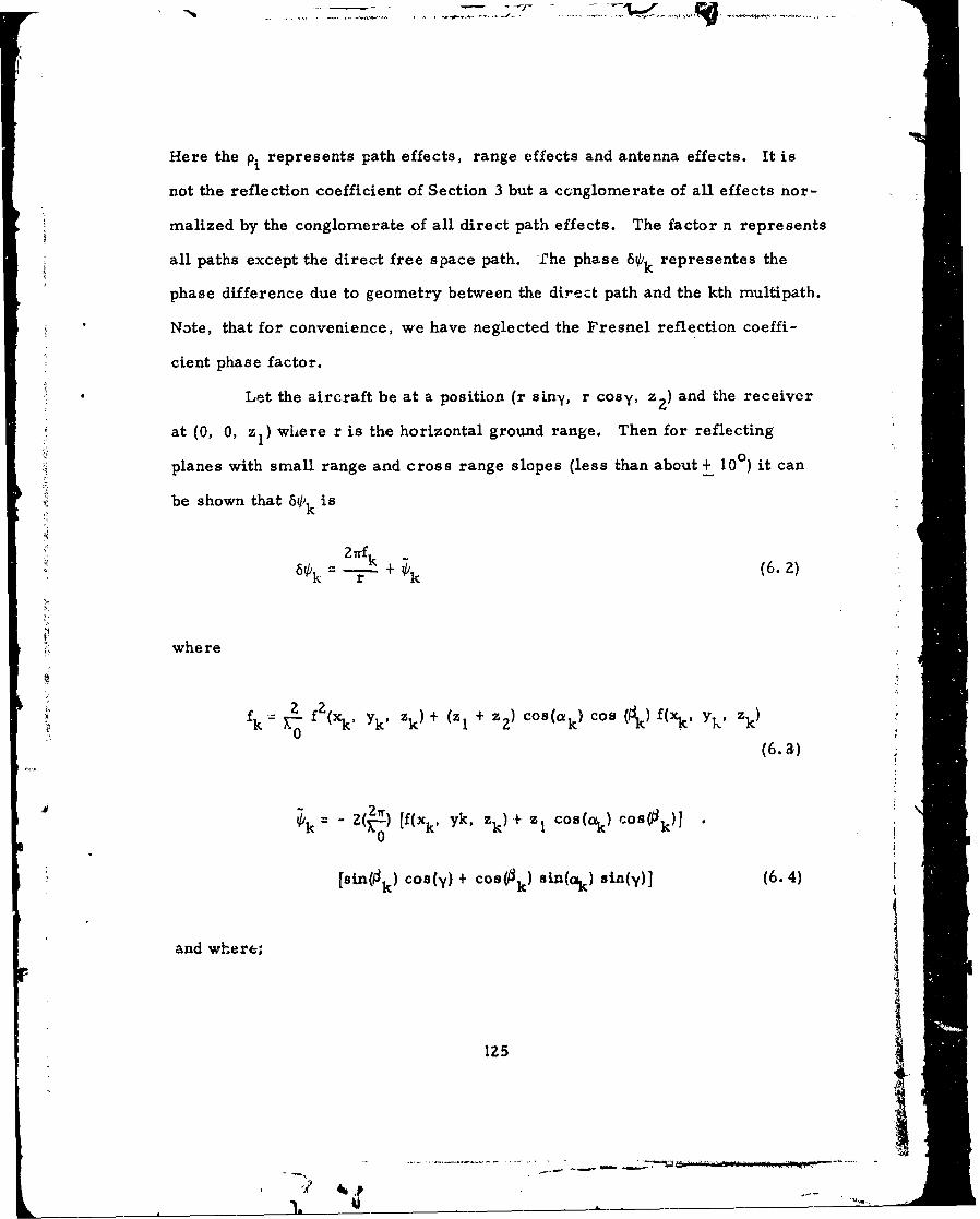
Here the pi represents path effects, range effects and antenna effects. It is
not the reflection coefficient of Section 3 but a conglomerate of all effects nor-
malized by the conglomerate of all direct path effects. The factor n represents
all paths except the direct free space path. The phase 65k representes the
phase difference due to geometry between the direct path and the kth multipath.
Note, that for convenience, we have neglected the Fresnel reflection coeffi-
cient phase factor.
Let the aircraft be at a position (r siny, r cosy, z2 ) and the receiver
at (0, 0, z1 ) where r is the horizontal ground range. Then for reflecting
planes with small range and cross range slopes (less than about + 10 it can
be shown that 6 0 is
• 2Mk
= + O'k (6.2)
where
Sk 37 f ( Yk' zk) + (z 1 + z2 ) cos(ak) cos ) f(xk. yV, zk)(6.3a)
Ok - Z(K-) [f(xk, yk, .k)+ z1 cos(ak) cos(ok)]0
:[sin (k) cos(y) + cos(#k) sLn(C'k) sin(y)] (6.4)
and where;HI
S__-- --
125. ,:,
f(Xk., Yk' Zk) - k sin(ok) cos{(k) + Yk sn(k)" Zk cos(ctk) cos(ok)' (6. 5)
Thus s2 is a periodic function of 1/r with frequencies fk' k 1,...
n, and phases 4k' k= 1,... n. Thus if s2is spectrum analyzed, fk and Ok can
be determined. It can be shown that by suitably varying y and z 2 the para-
kmeters k' 0.k and f(xk, yk' zk) can be obtained. The three parameters uni-
quely define the kth specular multipath source.
In Section 3, Fig. 19, we plotted a return with n = 2 as a function of
1/r. The multiple sinusoids were quite evident. We have plotted in Fig. 54
the real part of the Fourier transform, in Fig. 55 the imaginary part and in
Fig. 56 the power spectrum of the range corrected waveform of Fig. 19. The
three peaks in the power spectrum are quite evident. The lower peak is due
to the ground reflection and the upper peak is due to the tilted plane reflection.
The central peak is a result of beating between these two multipath signals.
6.3 ANTENNA DESIGN
The effects of multipath strongly impact on the choice of an antenna for
DABS. The discussion of azimuth estimation performance in Section 3 demon-
strated that the effect of loss of SNR could be quite serious. This loss was due to
the coherent interference between the direct path and the vertical lobing path.
This effect can be lessened by using an antenna with vertical aperture which
in effect will have a cutoff below the horizon. That is, the signal coming in
at negatlve elevation angles will be attenuated. This results in an effective
decrease in the reflection coefficient and increase in minimum SNR.
12(

{-4 -158171] - -0.00 150
0.00100
I-
w 0.00050
0
0 0.2 0.4 0.6 0.8
FREQUENCY
FI
Fig. 54. Real part )f Fourier transform.
127
Li n•'-- _

0.001I00.001
.• -0,001
-0.002
"""0-r- v . .• ' , " ' -t r--- --- r- --- r__ , ,0.2 0.4 0.6 0.8
FREQUENCY
F•
Fig. 55. Itmaginary part of Fourier transform.
128
i ,

I;:
0.002
0.001
0 0.2 0.4 0.6 0.8 1.0
FREQUENCY
Fig. 56. Power spectrum.
129

Other effects can also be studied. For example, the choice of hori-
zontal aperture and the nature of the sidelobes is also influenced by the type
of multipath present.
6.4 SIGNAL PROCESSING
The fade margins can be determined by the depths of the nulls that
occur. If these nulls are quite large then more sophisticated methods of cod-
ing and signal processing techniques will be necessary.
6.5 SITING
An important issue in the determination. of the implementation of a
DABS sensor is its siting. For example, where should it be, how high, and
what type of tilts should be used. The effect of specular multipath on these
issues is significant. Signal fading and coverage as well as angle estimation
performance are often dominated by the multipath environment. At the pre-
sent, there seems to be no cohesive measure of optimum siting performance
but possibly, through a detailed study of the many multipath effects, one may
evolve.
6.6 CONCLUSIONS
The models that we have proposed and e-veloped can be used to eval-
uate and aiialyze the effects of multipath on system performance and design.
Specifically, as we have observed, the effects of specular and diffuse multi-
path on azimuth errors can be evaluated in detail. Furthermore, link relia-
bility can be deteriorated by specular fading. The effects of antenna gains
and cutoffs in eliminating deep fades and serious azimuth errors can be ascer-
tained.
130
A,-

The localization algorithm has been found to provide a vseful tool
in determining the source of specular returns. By the nature of the signal
processing involved an effective increat;e in aperture can be obtained thus
increasing resolucion. The use Gf this technique on the analysis of DABSEF
data is presently under way.
1!
131
if,
SECTION SEVEN
-CQNC LUSIONS
The ability to obtain azimuth information and communicate data over
an air-to-ground surveillance link depends quite strongly on the different
types of multipath effects. To determine the influence oi multipath, we have
in this report, developed models for the signals that are received after having
propagated over multipath channels. The models include the effects of the
topographical and electrical properties of the reflecting surfaces as well as
the position of aircraft and sensor.
As a result of this study we have reached the following set of conclu-
sions:
1. The most serious cause of azimuth angle of arrival estimate
errors at the ground terminal will be specular multipath sig-
nals in the main beam. These will tend to cause bias errors
in the estimate. The seriousness of the errors as measured
by their magnitude will depend upon the angle made by the ray
from thi aircraft to the multipath reflecting surface and the
beam pattern of the receiving antenna. If this angle is small,
then the Fresnel reflection coefficient may be near unity which
can only be reduced by the antenna pattern. The magnitude of
the- azimuth estimation error also depends on the total phase
difference between the direct path and the reflected path. This
iii

can be obtained from the geometry of the aircraft, sensor and
reflecting surface.
The time delays for main beam multipath may vary signi-
ficantly, from a few nanoseconds to several microseconds, as
observed from DABSEF data. Again, this depends upon geome-
trical considerations. The nature of the surface will also affec*
the reflected signal. By using the concept of Fresnel zones, dif-
fraction effects can be included in a first order manner.
2. Diffuse multipath will have a minimal effect upon ground ter-
minal direction finding accuracy. The analysis of Section 4
has shown that diffuse multipath azimuth errors, as measured
in standard deviations, have magnitudes less than noise errors.
Furthermore, it has been shown by McGarty [1] that diffuse
multipath in certain cases contains information on the azimuth
of the target. This is in sharp contrast to the analysis of
R•ulke, et al., who employed results from Barton and Ward to
compute the deleterious effect of diffuse multipath.
3. For most cases of interest, neither specular nor diffuse multi-
path will seriously limit either the direction finding or communi-
cation capabilities of DABS. There are certain pathological
situations concerning specular multipath however, in which the
effect will be quite deleterious. These have been analyzed in
detail by McAulay. A
133
4.

4. The second order effects, such as shadowing and multiple
oriented suraces, could possibly dominate the signal behavior
at low angles. To answer this question adequately, extensive
experimental data are necessary.
As a result of the preceeding analysis it becomes evident that a sub-
stantial experimental program should be initiated to provide a data base
against which the proposed models can be compared. Part of this program
is included in the DABSEF (DABS Experimental Facility) presently in opera-
tion at Lincoln Laboratory. A more extensive program is also envisioned
which would include a portable system.
134
/•
S... •- -} . . .. .. "o•. . 1 .22 -.T . .. ... . .. • .,,,• ...

APPENDIX I
In the Appendix, we evaluate in closed form the bounding ellipse dis-
cussed in Section 4. Further, we relate this to several other physical para-
meters, namely, the minimum distance between the source and the receiver
via a multipath reflection. The basic equality to evaluate the ellipse, which
represents the locus of all points on the scattering plane whose total path
length from receiver to transmitter is p, is;
R1 + R 2 = p (I.1)
where R and R2 are given by (4.13) and (4. 14) respectively, and p equals ct.
Now rearrangeing and squaring, we obtain
R 2 = 2 - 2p R2 + R2 (1.2)
Substituting the values for these quantities we obtain,
x 2+ + z = P 2 P -Y) + (2 + z 2
2 2 2 2(13+ y2+ X 2yr+ r2+ z (L 3)
Cancelling and rearranging, we obtain
135

2p (ry) 2 + + z2 2 r2 - 2yr. (1.4)
Squaring yields
4p2 (r -y) 2 + x 2 + Z2] (p2 - z1 + z2+ r 4yr P z �+ r2 4y 2 r
(I. 5)
Now,
ZZ ZZ 2 12 2 Z Z4 p y - 4r y - 8p ry+ 4(p2+ z2 - z1 + r ry
+ 4p 2 r2+ 4p 2 x 2 + 4p2 z
= 2 2 2)2 (1.6)
Clearly, this is the equation of an ellipse. Completing the square, we can
obtain
2 2"22,4 (p 2 .r 2 ) Y + ( 4 p r + 2. ( I " + r ,
4(2 _ r)
2 Zp -z 2 z1 rr
22\"42r2 " 4 p2 z2Z
+ 4p 2 r + 2p(p2 + z- z+ r))2/(4(p r
(1.7)
136
/
. it-
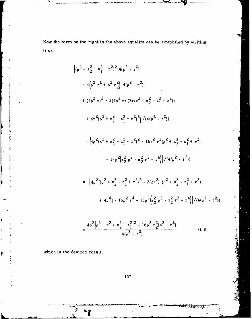
Now the term on the right in the above equality can be simplified by writing
it as
I(P2 + z2 - + r 2 )2 4(p 2 r 2 )
* 4 2 z +2)4 2 _ r 2
+"4p + r -2 2 2 z2+ (4pr)- 2(4p r) (Zr (c+z +r
2 2 2 2 221+4r(P+ +z 2 z 1 + r)/(4(p2 - r
[4PZ2 + - z2 z2 r2)2 16p 2 rz2(p 2 r2) z2
+16pz -z2 rZ - /4(p2 r'))
[4 2 2 2 + 2 2 2 2 2
4p 2[(pl + z2 z 2 -22(Zr 2 (P? +z 2 z z+r)2
4 2 4 2/z2 2 2 4")tf4
+4r j- 16 p r -16p z2 r2 r /(4(1 ~p' - r')
2 2
-(p r
r •which is the desired result.
137
-''• -'-- a-"

Now we can ask the question, where is the point at which the mini-
mum time ray touches the surface? That is for a given p, the time from
source to receiver is (R 1 - R 2 )/c. We first want to find the value of x which
minimizes this expression. By standard differentiation techniques we obtain
rz 1x r z . (I. 9) -
min z1 + z (
Note that if z1 z., then Xmin = d/2. Now the time it takes to cover this mini-
mum distance is to, where
2 22t + (z1 z2 (I. 10)
0 c
Compare this to the time between receiver and transmitter, tr,
12 2Vd•+ (z2 -z"Z)2 I l
tr c -1
Now att=to, pequals c to.
Then substitution into r 0 yields r 0 equal tG zero and x0 equal to Xmtn.
Thus as t increases beyond t the ellipse forms and grows.
138
138m
L ~ . ~ .. lmAlm

GLOSSARY OF TERMS
A - antenna area
AF - area of first Fresnel zone
A. - area of ith reflector1
A(t) irradiated area
b(e, *) - complex envelope of time invariant portion of diffuse field
b(O, 4, t) - complex envelope of diffuse field
c - velocity of propagation
d. - distance to ith dipole
d - interdipole spacing
D - divergence factor
Ef I - expectation
erf ( ) - error function
E- energy of transmitted signal
E- scattered field
fk - frequency of multipath interference
f(t) - complex envelope of transmitted signal
f(xk' Yk' zk) - displacement of kth multipath plane
G(0, -) antenna gain
GA(, A(0 difference antenna gain
GZ(8, 4) - sum antenna gain _
in(- Bes sel function
139
F"2 • ., .... . Jl

J(_) current density
k monopulse slope
k plane wave vector
kxik - components of propagation vectory
k
K(O) - channel spread function; azimuth only
K(O, p) channel spread function
' K (r, r) - covariance of diffuse signal5--
MGr.) - array delay vector
MID - multipath-interference detector
N - number of array elements
N - number of specular reflectors
n - normal vector
n(t) - complex envelope of receiver noise
nA - average number of scatterersN
o0-- noise spectral density
P - power of transmitter
Pi scattering plane septuple
R ground range
R( ) - reflection coeffeclent
R - radius of earthe
Rh range to horizon
R range to ith signal
1404I
S... ... -a - - -• - -
i,,i _'l•v~l••kl' -

RT range from aircraft to antenna
Rli - distance from receiver to ith scattering point
rn Zi - distance from transmitter to ith scattering point
r - range
r - point in space
r(t) complex envelope of received signal
- scattering plane displacement
4l- location of receiver
-r2 location of transmittec
- offset displacement of ith plane
S - scattering surface
SS(t01 1 2) - shadowing functions
S(t) - power density at receiver
s - magnitude of power received
s (t) - transmitted signal
s(t) - complex envelope of transmitted signal
s(r) - complex envelope of time invariant diffuse signal
s(r, t) - complex envelope of time variance diffuse signal
SNR - signal-to-noise ratio
t - time
t- signal emission time of source
t transmission time from transmitter to reteiver
t transit time of scattered path
141 -s •a- -- ' * ---VilIi

v1 vector to image antenna
V vector to transmitter-2v3 - vector to receiver
var (- variance
x- half width of first Fresnel zone
- antenna phase center locationYl
z 1 antenna height
x2
YZ - location of aircraft
z2.
YO- center of first Fresnel zone on y a-ds
z(X, Y) - random surface
a- cross-range tilt
- range tilt
r(r, r - Greens function
y - noise-to-signal ratio
- difference signal
A 1 deviation of first Fresnel zone from yo
V - del operator (gradient or divergence)
6(k - k') - delta function
E - dielectric constant of Ith scatterlng.plane
- diffuse multipath to free space signal r-tio
'A-i aperture reflection factor
142
.4 4b- -. -- i--
2 $

QD. -diffuse reflection factor1
YF. - Fresnel reflection factor
1
- - azimuth e -imate
0 B - beamwidth
- azimuth of ith signal
-0 free space wavelength
- directioa cosine
-B beamwidth
- interference-to-signal ratio
Pi ith reflection coefficient
- sum signal
r(t) - magnitude of time -ariation of power received
4 b - channel attenuation coefficient
h - standard deviation of surface height
2
T- diffuse signal energy
2T 2 - power in diffuse field
- scattering cross-section
S- conductivity of ith scattering plane
- correlation length of surface
2r2- noise covariancen
2* a2 signal energy
T(s s i) " scattering cross sections
143

- variance of azimuth estimate
2- variance of
T - multipath-interference statistic
- elevation (incident or ith signal)
- selevation of scattered signal
•F. - phase due to Fresnel reflection
phase difference
k - multipath phase
R. - phase due to rangeII
w - carrier frequency
() - array ambiguity function
- transformation matrix
144
/.

-vE
REFERENCES
Ament, W.S.[1] "Toward a Theory of Reflection by a Rough Surface," Proc. IRE,
41, (1953) pp. 142-146.
[2] "Forward and Back-Scattering From Certain Rough Surfaces,"IRE, AP-4, (1965) pp. 369-373.
Barrick, D.E.
[1] "Rough Surface Scattering Based on the Specular Point Theory,"IEEE, AP-16, No. 4, (July 1968) pp. 449-454.
[2] "Unacceptable Weight Correlation Coefficients and the Quasi-Specular Component in Rough Surface Scattering, " Radio ScienceVol. 5, No. 4, (April 1970) pp. 647-654.
[3] "Theory of HF and UHF Propagation Across the Rough Sea,"Radio Science, Vol. 6, No. 5, (May 1971).
Barrick D.E., Peake, W.H.
[1] "A Review of Scattering From Surfaces with Different RoughnessScales, " Radio Science, Vol. 3, No. 8, (August 1968) pp. 865-868.
Barton, D.K,, Ward, H.R.
[1] Handbook of Radar Measurement, (Prentice-Hall, Englewood Cliffs,N.J. , 1969).
Bass, F.G., etal.
[1] "Very High Frequency Radio Wave Scattering by a Distributed SeaSurface Pt. I, "IEEE, Vol. AP-16, No. 5, (Sept. 1968) pp. 554-559.
[2] "Very High Frequency Radio Wave Scattering by a Distributed SeaSurface Pt. I1, " IEEE, Vol. AP-16, No. 5 pp. 560-588.
Beard, C.I.
[1] "Coherent and Incoherent Scattering of Microwaves from the OceanIEEE, Voi. AP-9, No. 5, (Sept. 1961) pp. 470-483.
[2] "Behavior of Non-Rayleigh Statistics of Microwave Forward Scatterfrom a Random Water Surface," IEEE, Vol. AP-15, No. 5(Sept. 1967) pp. 649-657.
145

Beard, .1., et al.
[1] "Phenomenological Vector Model of Microwave Reflection from theOcean, "IRE, Vol. AP-4, (1956) pp. 162-167.
Beckmann, P.
"[1] "Scattering by Composite Rough Surfaces, " Proc. IEEE,(Aug. 1965) pp. 1012-1015.
[2] "Scattering of Light by Rough Surfaces, " Progress in Optics,IV, (E. Wolf, Ed., J. Wiley, N.Y., 1967) pp. 55-70.
[3] "Shadowing of Random Rough Surfaces, "IEEE, AP-14, (1965)pp. 384-388.
Beckmann, P., Spizzichino, A.
[1] The Scattering of Electromagnetic Waves from Rough Surfaces,(Permagon, N.Y., 1963).
Brockelmann, R.A., Hagfors, J.
[1] "Note on the Effect of Shadowing on the Backscattering of Wavesfrom a Random Rough Surface, IEEE, Vol. AP-14, No. 5,(Sept. 1966) pp. 621-629.
Clarke, R.H., Hendry, G. O.
[1] "Prediction and Measurement of the Coherent and IncoherentPower Reflected from a Rough Surface, IEEE, Vol. AP-13,No. 3, (1964) pp. 353-363.
DeLorenzo, J.D., Cassedy, E.S.
[1] "A Study of the Mechanism of Sea Surface Scatcering, " IEEE,Vol. AP-14, No. 15, (Sept. 1966) pp. 611-620.
Eckart, C.
[1] "The Scattering of Sound from the Sea Surface, " J. A. S. A.,Vol. 25, No, 3 (May 1953) pp. 566-570.
Fung, A.K., Moore, R.K.
[1] "The Correlation Function in Kirchoff s Method of Solution ofScattering of Waves from Statistically Rough Surfaces," J. Geo.Res., Vol. 71, No. 12, (June 1966) pp. 2939-Z943.
Furutsu, Kf
[1] "A Statistical Theory of RIeie Diffraction," Radio Sci., Vol. 1,No. 1, (Jan. 1966) pp. 79-98.
146
V•
"L '

Hagfors, T.
[1) "Backscattering from an Undulating Surface with Applications toRadar Return from the Moon, " J. Geo. Res., Vol. 69, No. 18,(Sept. 1964) pp. 3779-3784.
Hayre, H.S., Moore, R.K.
[1J "Theoretical Scattering Coefficient for Near Vertical Incidencefrom Contour Maps, " J-ur. Res. Nat. Bur. Sts., Series D,Vol. 65D, No. 5, (Sept. -Oct. 1961) pp. 427-432.
Hoffman, W. C.
[11 "Scattering of Electromagnetic Waves from a Random Surface,"Quant. Appi. Math., 13, (1955) pp. 291-304.
Jordan, E.C., Balmain, K.G.
[1] Electromagnetic Waves and Radiating Systems, (Prentice Hall,Englewood Cliffs, N.J., 1968).
Kerr, D.E.
[1] Propagation of Short Radio Waves, (Dover, N.Y., 1965).
Kodis, R.D.
[1] "A Note on the Theory of Scattering from an Irregular Surface,"IEEE, Vol. AP-14, No. 1, (Jan. 1966) pp. 77-82.
Lonquet-Higgins, M. S.
[1] "Reflection and Refraction at a Random Moving Surface, Pt I, "J. 0. S.A., Vol. 50., No. 9, (Sept. 1960) pp. 838-844.
[23 "Reflection and Refraction at a Random Moving Surface, Pt. II,,J. 0. S. A., Vol. 5, No. 9, (Sept. 1960) pp. 845-850.
Maltz, F.H., Meecham, W.C.
[11 "The Effect f Curvature Variations on the Scattering from RoughSurfaces," 2. Stat. Phy., Vol. 3, No. 4, (1971) pp. 385-394.
McAulay, R.J.
[13 "The Effects of Interference on Monopulse Performance" LincolnLabortory, M.I.T., Technical Note, TN-1973-30, (1 Aug. 1973)ESD-TA-73-176.
McAulay, R. J., McGarty, T. P.
[13 "An Optimum Interference Detector for DABS Monopulse DataEditing," Lincoln Laboratory M.I.T. Technical Note, TN-1973-48(26 Sept. 1973) ESD-TR-73-253.
147
, / ' .,,

McGarty, T.P.
[11] "Azimuth-Elevation Estimation Performance of A SpatiallyDispersive Channel, " IEEE Vol. AES-10, No. 1 (January 1974)pp. 58-69.
Mitzner, K. M
[1] "Change in Polarization on Reflection fromn a Tilted Plane, " Rad.Sci. Vol. 1, No. 1, (Jan. 1966) pp. 27-29.
Rice, S.O.
[1] "Reflection of Electromagnetic Waves from Slightly Rough Surfaces,"Comm. Pare & Appl. Math, 4, (1951) pp. 351-378.
Silver, S.
[1] Microwave Antenna Theory and Design, (Dover, N.Y., 1965).
Smith, B.G.
[11 "Geometrical Shadowing of a Random Rough Surface, " IEEE,Vol. AP-15, No. 3, (Sept. 1967) pp. 668-671.
Spingler, G.F.
[1] "Analysis of Side-Lobe Suppression Capabilities at Joint-Use RadarBeacon Sites," FAA Report No. RD-67-59.
Stratton, J.A.
[1] Electromagnetic Theory, (McGraw Hill, N.Y., 1941).
Twersky, V.
[I] "Reflection Coefficients for Certain Rough Surfaces, " J. App. Phys.,24, (1953) pp. 659-660.
[2] "Certain Transmission and Reflection Theorems, " J. App. Phys.,Vol. 25, No. 7, (July 1954) pp. 859-862.
[3] 'On the Scattering and Reflection of Sound by Rough Surfaces,"J.A.S.A. Vol. 29, No. 2, (Feb. 1957) pp. 209-225.
[4] "On Scattering and Reflection of Electromagnetic Waves from RoughSurfacbs, " IRE, AP-5, (1957) pp. 81-90.
Van Trees, H. L.
[1] Detection Estimation and Modulation Theory, Pt. m, (J. Wiley, N.Y.1971).
Venetsanopoulos, A.N., Tuteur, F.B.
[1] "Stochastic -Filter Modeling for the Sea-Surface Scattering Channel,
J.A.S.A., 49, (1971) pp. 1100-11007.
148
! -
I *..!
-2

Wagner, R. J.
[1] "Shadowing of Randomly Rough Surfaces," J.A.S.A., Vol. 41,No. 1, (1967) pp. 138-147.
Yaglom, A. M.
[1] "Second-order Homogneous Random Fields, " Proc. 4th BerkeleySymp. Math. Stat. and Prob. 2, pp. 593-620.
II
-1
•i
149
SU.S. OOVE4MENT PPNTONG OFFICE! W94 74-195 -0
* 4b