ad-aq27 958 chapacteristic steady-state electron emission properties ... · pdf...

This Document

Reproduced FromBest Available Copy

UV. W•APTBENT OF CWIEACEN TeMWo tatuad" Km O

AD-AQ27 958

CHAPACTERISTIC STEADY-STATE ELECTRON EMISSION

PROPERTIES FOR PARAMETRIC BLACKBODY X-RAYSPECTRA ON SEVERAL MATERIALS

MISSION RESEARCH CORPORATION

PREPARED FOR

DEFENSE NUCLEAR AGENCY

FEBRUARY 1976

REPRODUCTION QUALITY NOTICE

This document is the best quality available. The copy furnished

to DTIC contained pages that may have the following qualityproblems:

"• Pages smaller or larger than normal.

"* Pages with background color or light colored printing.

"* Pages with small type or poor printing; and or

"• Pages with continuous tone material or color

photographs.

Due to various output media available these conditions may ormay not cause poor legibility in the microfiche or hardcopy outputyou receive.

D7 If this block is checked, the copy furnished to DTICcontained pages with color printing, that when reproduced inBlack and White, may change detail of the original copy.

224208

DNA 3931T

CHARACTERISTIC STEADY-STATEELECTRON EMISSION PROPERTIES FOR

oC PARAMETRIC BLACKBODY X-RAY•2 SPECTRA ON SEVERAL MATERIALS

-,,e Mission Research Corporation

735 State Street

C' Santa Barbara. California 93101

e• February 1976

Topical Report

CONTRACT No. DNA 001-76-C-0086

' APPROVlD F0R PUGLIC RELEASE;Dt-SVTRIGUTIOM UNLIMITED.

TmS ORK SPONSOPE• BY THE CIEFFNSF NUCLEAR AGENCYULNieR RCT&F RMSS CODE 0227C;'6464 R99QAXB0 964 H2!00.

Prepared for

Director

DEFENSE NUCLEAR AGENCY

Washington. 0. C. 20305

* IIstmgld v 21NATIONAL T!C04NCAL

NEORMATION SeRViC

UNCLASSIFIEDSlCUIIV?. CL A$SIrICATIO% Or TNIS PAGE PWhw. not& Fnpd'¢

REPORT DOCUMENTATION PAGE IEADINLTRUCT FORM

IRPORT %jMRt" I. GOVT ACCESSION NO, J Z T U a

DNA 3931T A

S'LTLr Will %r-,hwfhft) 5 TyVP. Or REPORT ph Pt1IOC D QýOvv'rF

CHARACTERISTIC STEADY-STATE ELECTRON EMISSIONPROPERTIES FOR PARAMETRIC BLACKBODY X-RAY Topical Repor"SPECTRA ON SEVERAL MATERIALS 6 PERFO.RING O.G REPORT ,-jM9LR

14RC-N-221 Revised7 Au'I..~oR- A CO)%-ACT 1) GRANT NUM9(a-

Neal j. Carron DNA O0i-76-C-OC6

9 F`E7r'QMtN(. 004CANIIATIO.4 -40AF AND AODRfSS 10 PRO(.1AM V1 1,F4 ~OPrr" 'A~iiaAE A A *O08. UNT Nu" ofrp,

Mission Research Corporation735 State Street NWED Subtask F?'-QAXE-,BO, 9-' hSanta Barbara. CalJfornia 93101

II CONTQOLLI4G OFFICE NAME ANO ADORESS 12 REPORT DATE

Director February 197,Defense Nuclear Agen,,y ,, Nu.•F'-O O PA , %

Washington, D.C. 20305 _ _ _ _

14 MoNt!OPINt, A'4(~N M A[DDAF5,,, ,1.? r. (Off-, I$ SF'"I -. AS¶ -f ~U11CLASSIFI ED

I-DECLA~SSIIC ATION DO*NGRADINGSC-'E OULF

Approved for public release: distribution unlimitv-d.

' ,TPI1UTIOd STATFMFN ,I 1h. .h.f.- .. i,..14n If ,,e :', I I-ff11-1 I-ff, Nfq,,, '

8 91UPPLEMFN"A•v NOTES

This work sponsored by the Defense Nucl-ar AF,-ný:y under RDT&• !RSS Cod'B32u7,1,, h 4 R9)QAXEpO, 9'1h H2590D.

14 WFV N1CROS t,,ma, ,i-v.,,e .r~,itr nfre .- ,,¶n% mitt n h%- 111-b. -

Nuclear Weapons E.f.cts Space-charge LimitingSGcalP BlackbodiesPhotoelectric Yield

'0 *8SRPAC7 ta ,r.- - ,-r -npIF , r if . mitt ltdr,,th P, Pita, b nt.-F-)

We collect together in this note certain photoelectric efficiencies.electron energy spectra. electron boundary lay--r plasma Debye lengths.f-lectron number densities, electric rields. and plasma frequencies prevailingin steady state when blackbody photon sources are incident on Aluminum, Gold.and Silicon Dioxide. Only backscattered electrons are considered. Thefigures presented allow quick estimates of many boundary layer properties.

DO I r)AN 1, 1473 OUNCLASSIFIED

I . SECURITY CLASSIrICATION Or TWIl. PAGE (WIl'..t P.. V ,4)

IJ

TABLE OF CONTENTS

PAGE

ILLUSTRATIONS 2

SECTION I.-INTRODUCTION 5

THEORETICAI ASSUMPTIONS 6

SECTION 2-ELECTRON YIELDS AND ENERGY SPECTRA 9

SECTION 3-TIMES OF VALIDII( OF STEADY-STATE THEORY 20

A. Transient Build-Up to Steady State 21

B. Maintenance of Quasi-Steady State 26

SECTION 4-DEBYE LENGTHS 31

SECTION 5-ELECi'RON NUMBER DENSITY AT SURFACE 36

SECTION 6-ELECTRON NUMBER DENSITY PROFILE 40

INTEGRATED NUMBER DENSITY 43

SECTION 7-ELECTRIC FIELD AT SURFACE 45

SECTION 8-ELECTPIC FIELD PROFILE 49

SECTION 9-PLASMA FREQUENCY AT SURFACE 5!.

SECTION 10-DIPOLE MOMENT PER UNIT AREA 55

SECTION 11-EXAMPLE 58

REFERENCES 62

[ . . . . .. . . . .. . . . . .

p.

LIST OF ILLUSTRATIONS

F IGURE PAGE

1 Total backscattered electron yield for incident blackbodyspectrum. 11

2 Electron spectra, 1 keV incident blackbody. 12


4 Electron spectra, 3 keY incident blackbody. 14


6 Electron spectra, 8 key incident blackbody. 16

7 Electron spectra, 10 key incident blackbody. 17

8 a. ts for Aluminum. 2

8 b. ts for Gold. 24

8 c. ts for Silicon Dioxide. 25

9 a. tret for Aluminum. 1,3

9 b. tret for Gold. 29

9 c. tret for Silicon Dioxide. 30

10 a. Debye lengths for Aluminum. 33

10 b. Debye lengths for Gold. 34

10 c. Debye lengths for Silicon Dioxide. 35

11 a. Surface eletron der.sity for Aluminum. 37

11 b. Surface ele,-.ron density for Gold. 382

'4. .

FIGURE PAGE

11 c. Surface electron density for Silicon Dioxide. 39

12 Normalized electron density profile. 41

13 Normalized electron density profile. 42

14 Fraction of electrons out to x. 44

is a. Surface electric field for Aluminum. 46

15 b. Surface electric field for Gold. 47

15 c. Surface electric field for Silicon Dioxide. 48

16 Normalized electric field profile. so

17 a. Surface plasma frequency for Aluminum. 52

17 b. Surface plasma frequency for Gold. 53

17 c. Surface plasma frequency for Silicon Dioxide. 54

18 Normalized dipole moment per unit area. 56

19 X-ray time history for illustrative example. 59

SECTION 1

INTRODUCTION

To estimate the properties of the electron boundary layer produced

when X rays fall on a material surface, it is helpful to have available

tabls and curves of' useful boundary layer properties when a parametric set

of photon spectra is incident on common materials.

This note collects some boundary layer properties for hackscattered

electrons for the cases in which blackbody photon sources of temperatures

kT = 1, 2, 3, 5, 8, and 10 keV are normally incident on aluminum, gold, and

silicon dioxide. For reasons discussed below the curves presented are for

the case of a steady-state boundary layer, that is, it is assumed that

conditions are not changing with time.

The eclectrc,i properties given 'are:

1. Photoelectric yield, and bckscattered electron energy

spectra (Section 2);

2. Conditions for which steady state theory is valid (Section 3);

3. Boundary layer Debye lengths (Section 4);

4. Electron number density at the surface (Section 5);

5. Electron number density profile and the integrated

density (Section 6);

6. Electric field at the surface (Section 7);

Pmrceding pap blank" 5~

I

7. Electric field profile (Section 8);

¶ 8. Plasma frequency at the surface (Section 9);

S9. Electric dipole moment per unit area (Section 10).

In Section 11 we give an example that illustrates the use of the

graphs.

The graphs given here are meant te provide the reader with a ready

reference for estimating boundary layer properties for incident photon

spectra approximating blackbodies when steady-state conditions are valid.

THEORETICAL ASSUMPTIONS

The exact conditions prevailing when an X-ray beam is incident on"

a material surface can vary widely. The incident photon pulse can have any

time history and any energy spectrum, and the energy spectrum can itself

vary with time. The angle of incidence and the physical size and shape of

the target can also vary widely.

It would clearly be a difficult and lengthy task to paraimetri:e

all of these variables, tantamount to solving the general problem. Hlere we

choose a more modest goal. We restrict attention to normal ang.es of

incidence, and targets that are flat surfaces with dimensions large compared

to the thickness of the boundary layer. This last assumption permits a one-

dimensional theoretical treoftment.

In addition, we choose for the energy spectrum a blackbody spectrum

independent of time. This is partly because of its universal availability

(theoretically) and similarity to some experimental sources of interest,

and partly because a blackbody photon spectrum produces a t)ackscattered

electron energy spectrum which is very nearly exponential (see Section 2),

6

I|

and the steady-state boundary layer structure for an exponential electron

spectrum is known,

A parametric study using monoenergetic X rays would 'not be particularly

useful unless one were actually interested in the response to monoenergetic

X rays. Since the boundary layer problem is a non-linear one, it is not pos-

sible to determine the response to a spectrum by superposing the responses

to monocnergetic photons.

Even with these restrictions, the photon source can have an arbi-

trary time history. The solution for the time-dependent boundary layer

structure even in one dimension is very difficult, and until a thorough

stud%- of this problem is made we find it wise to restrict parametric studies'

to the time-independent, or steady-state, case. Many photon sources of

interest, while varying with time, vary slowly enough so that steady-state

theory is approximately applicable at every instant of time using the

instantaneous value of the X-ray flux.

Hence, in spite of the above stated restrictions, the graphs

presented in this report should be useful for estimating boundary layer

properties in many experimental situations of interest.

We have mentioned that a blackbody phuton spectrum produces'a

backscattered electron enerýy spectrum that is very nearly exponential. It

also turns out that the electron angular distribution is very nearly a cosO

distribut ion. The steady-state boundary layer theory for this case of

exponential energy spectrum and cosO angular distribution was presented in

Reference. I. The graphs in the present report were constructed from the

formulae given there.

7

In Figures 8, 9, 10, 11, 15, and 17, information has beencompressed by using the top and right scales as well as the, bottom and left

scales. The top scale should be used with the right scale, and the bottom

scale should be used with the left scale.

Bi

SECTION 2

ELECTRON YIELDS AND ENERGY SPECTRA

The backscattered electron yields and energy spectra depend only

on the X-ray energy spectrum and angle of incidence and on the surface

material. (For a thin surface they also depend on the material thickness.

Here we assume the material is at least one electron range thick, and

they are therefore independent of thickness.) They do not depend on the

X-ray time history, and hence can be discussed independently of any

dynamical assumptions about the boundary layer.

The photoelectric yields and backscattered electron energy spectra

were computed using the electron transport code QUICKE2 2 . The photoelectric

yields (or "efficiencies") are listed in Table 1 in units ofelectrons per

photon and in units of electrons per calorie of incident fluence. These

same backscattered yields are shown as a continuous function of incident

blackbody temperature in Figure 1 (in units of electrons per calorie only).

The backscattered electron energy distributions are shown in

Figures 2 through 7 for the six blackbody te-mperatures chosen. The

ordinates are in units of electrons/keV per calorie incident fluence.

Figures 2 through 7 are partially smoothed from the output of QUICKE2.

It is seen from these figures that, except for certain jumps at

low energies caused by Auger electrons (at 1.4 kcV in Aluminum and 8.25

keV in Gold), the electron energy spectra are nearly exponential with some

characteristic energy E1 ,

9

X -~ -ý -cl- -

V). Cai- 00J k5

4-J

4- U i C~l t2- tn m- if

I-,~CC

Gaw *Oco Cu (n LO. -P (

W oo (_ _ __ _ _ _ __ _ _ _

4 )0 41- -

..Cr C\J M'. CJ NJ N\ '%

Iti '. O Ifl CO '-v L I~) LCI j (~I C)

Ga w cu5- - - - .-EGa Ga

LO D n .'r.4-'l

CL 0 c'4j- u

-0 f

.10

I14 * j * . ... ... .. -.

.4J0

iQii

121

S. .. .. .. . . . . . . .

, . . . . .. .. . . . . . . . . .. . . .

.. ...... .. .i 2• .... ... ...... . . ..- --,-.. ., ... . . .. . . . . . . .. . . .. . ...

% u 10 3 il I I- -I"0 1 2 ... 4 5 6 7 8. 9 TO."2

Incden Blacbod.Temera.re...V

Figure ~ ~ ~ ~ ~ ~ -.. 1.Ttl--.ctee eeto ildfricdetbakod.pcrm

,• .• * 6 - --• -° . . .. . . .-.

i. . . . . . . . . . ..

13 - ... KT I keV

10

" A...il ; 'T * . -. I . . .. . . ..

"I-

., I . . . . . . . . . . . . . .. .. .

01210 .

0~

S22 : '. . . . . . • . . . . . .

4.)

CLJ

0u . . . . . . . . . . - . . . . . .•

Si A Au

109

10 - - - *- -- - -

0 5 1015 20 z 5

Electron Energy (key)

Figure 2. Electron spectra, 1 keV incident blackbody.

12

It

4 4 •4

.1. .

1 01 ... ... ... ........ ........ . .4 . . . . . . . . . . .

012 11'

Au

10 11A.... ......o ,I '4-

.~ .44 .... .4, . ., . 4. 4 .4 . .101 .... ' . .......... - - - -

1 o 1 ' 1 TTTk - 7 . 4 . -1

. .. .. . . .. . .

10 0 ' 1-

Electron Energy (keV)

Figure 3. Electron spectra, 2 key incident blackbody.

13

L

1013 "KT 3 kPV

io 2 I , - - - - - .

..... .. . . . . .

..u . .... ... .. . . .

. . . . . . . . .

12

L

Ail A Au I" I l

T o

00

- 4U

- 1

0 10 20 30 40 50


Figure 4. Electron spectra, 3 ',V incident blackbody.

14

. . . ... . . .

I; 4 KT 5 keV ....

10l ,io Au , ,

19.104

4J '4 8

f o . I Ll i i

OJt

Fiur 5. Elcto spcr,5k icietbakoy

I I15

o12 KT 8keV

1~~~' 4 1I___ __

116

I 41 I1 I I" I " .1 1 t i l : I ! ,,

12 'KT 10 keV

, * - , , .* ,4

1010 - -

10

. . .... .. ..

!.. .

Au

10,S2.. A . ..........

S. .. ....... ' • . .4 ,4

0 10 20 30 40 50 60 0 I 90 100


Figure 7. Electron spectra, 10 keV incident blackbody.

17

dn "E/EI

dE. , C electrons/keV/unit fluence

where E is the electron energy. By fitting a straight line to Figures 2

through 7, ignoring the Auger edges, we have determined values for E11Those are listed in Table 2. 'rho energies E 1 are not very different from

the temperature KT, and are nearly independent of target material. Using

electron energy spectral response to monoenergetic photons, and superposing

a blackbody spectrum, it is not hard to show that the electron spectrum

should indeed be nearly exponential with exponentiation energy approximately

equal to KT, as has been discussed by Higgins .

i !i• . 18

Table 2. Exponentiation energies, El, forbackscattered electrons.

Incident PhotonBlackbody Exponentiation Energy. E, (keV)

Temperature .. .

(keV) Aluminum Gold Silicon Dioxide

-1 1.2 1.01 0.98

2 9.09 2,05 1.97

3 2.9r, 2.99 2.86

5 4.77 4.A7 41.63

8 7.27 7.95 ',. ,..

10 8.69 10.07 8.36

19

SECTION 3

TIMES OF VALIDITY OF STEADY-STATE THEORY

For a given X-ray pulse there are two characteristic times that

determine whether or not steady-state theory is applicable.

The first electrons ejected by the arriving X-ray pulse arecertainly not in steady state. Some time, t., must pass after the X rays

first arrive before the boundary layer will have achieved a steady" or quasi-

steady state. There will be a transient build-up to steady state. We may

expect this time t to depend on the fluence and the rise time of the

incident pulse.

Once this transient build-up is over, we will achieve a steady

state and stay in a (quasi-) steady state only if the X-ray pulse is not

changing too rapidly in time. Each ejected electron takes a certain time,

t rt' to reach its maximum distance from the surface, turn around, and

return to the surface. Steady-state formulae will be applicable after time

ts only if the incident puisr changes only slightly during thL time trot

that it takes an electron of, say, average energy to return. Thus the

boundary layer will maintain a (quasi-) steady-state structure with the

instantaneous value of the flux only if the flux is nearly constant over

the lime trt.

Hence, for a given pulse time history, one must estimate both t

and t ret' We now discuss these two times more quantitatively.

20

A. Transient Build-Up to Steady State

Let c(t) be the X-ray fluence [cal/cmI2 that has arrived up to

time t. Then the X-ray flux is

= d- [cal/cm-/sec] (1)dt

Let Y [electrons/cal] be the photoelectric yield as given in Table I or

Figure 1. Then electrons are emitted at a rate

r 0 Y-) Ielectruns!cm-/;ec] , (2)

andt

N(t) fJr 0 dt [electrons/cm] , (3)

0

are emitted bN time t.

Now Reference 1 shows that, for an exponential electron energy

spectrum with exponentiation energy El and a cosO angular distribution, the

number of electrons required for steady state when the emission rate is r

is

Ns = (r= 0 V 3EI- .T e 2 ) 1/2 [electrons/cm] (4)

Steady state theory should begin to apply after the number of

electrons ejected, Equation 3, exceeds that necessary for steady state,

Equation 4. Hlence, equating N(t) and N will determine the time t sS 5

To simplify matters we assume the pulse is linearly rising,

= -- , (5)

at a rate p [cal/cm2/sec2], so that

21

N(t) y t~,2 ,(6)

2

and

"s " 3V'e 2 (7)

Equating these we obtain

1/3

2(

This is plotted as a function of [ [cal/cm /nanosec in Figures

8a, b, and c for aluminum, gold, and silicon dioxide.

For exampl , if a 3 keV blackbody falls on gold and has a rise

rate of 10"6 cal/cm /ns", then Figure 8b shows ts = 6 ns.

Actually some of the electrons emitted by time ts, Equations 3 or

6, will have returned so that the total number of electrons residing outside

the surface at t will be less than N(ts). Hence it will take somewhat

longer than ts as given by Equation 8 before steady-state theory is fully

applicable.

In addition, electrons emitted with energy less than E1 will be

in steady state before ts since their return time is less than that for

electrons of energy E . Similarly, more energetic electrons than E will

take longer to achieve steady state. Thus if one is interested in certain

details of the boundary layer that depend on high energy electrons, such as

the local electron number density far from the surface, one must wait

22

*-a. S,

ý4ca1/cm2 /nanosec2

100

0.i0

0 00V

10,

10-1 -

100

ý[ca 1/cm2 nnsc

Figure 8a, for Al uminum.

Numbers on curves are blackbody temperatures in keV.

23

$tfcal/m 2 /nanosec2]

100

11

1 0

ý4ca1/cm2 /nanosec2 I

Figure 8b. tsfor Gold.


24

ý[Ica1cm 2 /nanasec 2 I

0 o1

10

2 2,[K1cm/anse

Figur 8c. for ilicn Dixide

252

longer than ts before trusting steady-state expressions. Hence the precise

value of t as given in Figures 8 must be used with care.

Fortunately many X-ray pulses last mt,!'h longer than t, so that

even with the above two caveat-; Figures S are useful.

In Figures Sa, b, and c, and all later figures marked with two

pairs of arrows, the left-hand scale should be read with the lower scale.

and the right-hand scale should be read with the upper scale.

B. Maintenance of Quasi-Steady State

Steady-state theory with thci instantaneous value of X-ray flux ,il!

remain applicable if the flux is nearly constant during the turn around

time, t, of an electron of average energy. From Referen,.: 1, we find

that an electron emitted with normal component of energy 1/2 m-, where v• X X

is its normal velocity, equal to the average energy E,

1 2m v= E)

will return in time

t ret V .

= \2mVl/- e- r 0 0(lt)

where is the surface Debve length and vi = t. 11sing Luation.

this can be written

"ret - .1- 8 10 3 (C1 i ) -e aIl

26

BEST AVAILABLE COPY

This• is shown as a function of the flux 1 d:/Jt Ical/cm'/nanosecl in

Figures 9a, h, and c.

For example if a S keV blackbody is illuminating aluminum at an

instantaneous flux of 10) cal/cm /nanosec, Figure 9a shows that steady-state

exprtssions should he %jlid if the flux does not change imch over a time

t *O. 0.4 nanosec.

Since electrons emitted with energy greater than EI will have a

longer return time, one must use a larger t ret if one is interested in

detailed steady-state quantities that depend on these higher energy

electrons, such as the local electron number density far from the surface.

If. however, one is interested in a qiiantity that is determined primarily

by lower energy electrons, such a% the local numher density less than a

l•,,e length from the surface, one may use a smaller t.

For "global" or integrated quantities such as the surface electric

field, (or, what is the same thing, the surface charge density or the total

number of electrons outside the surface) the time tret plotted in Figures

9a, b, and c should he adequate.

From the given properties of the incident X-ray pulse one can

determine t5 and tret from Figures A and 9. The graphs in the following

sections will he valid for times greater than t if the flux is nearly con-

stant over a time t

ret•

27

X-ray Flux, ýIcal/cm2I/nanosecl

Aluminum -: 0

~10 101

10

X-ray Flux, lcl/n 2/aosc

Figure 9a. t ret for Aluminum.

Numbers on curves are blackbody temperatures in key.

28

X-ray Flux, ý[cal/cm2/nanosecI

io0 10

2: :~ 1.F

10

Figur 10 rtfo od


29

X-ray Flux.i, Ncal/cm 2/nanosec]

S3ilicon Dioxide 101

I-

X-a lufca/m/nnsc

Fiu0 9c1rtfo iionDoie

Nubrtncre r lckoytmeaue nkV

30

SECTION 4

DEBYE LENGTHS

The L)ebye length is the characteristic distance over which the

properties of the boundary layer vary significantly. It is a measure of

the "thickness" of the boundary layer. If w is a characteristic energy

(ergs) of a plasma, and N is the electron number density (cm-3) then the

I)ebyc length isw

z D cm (12)

It is equal to a characteristic plasina velocity divided by the plasma

frequency.

In the present context we use for w the exponentiation energy E.

'rhis is also the average electron energy. For N we take the value at the

emission surface in steady' state when the electron energy distribution is

exponential and the angular emission distribution is cosý'• In this case

N = o (13)

where .v = Y21-E/m and r 0 is given by Ecuation 2. Thus

(16 Ti/2 e 2

1 (cm ns

31

These Debye lengths are those appropriate for the plasma at the

material surface in steady state including the returning electrons. Since

the local average electron energy divided by the number density increases

with increasing distance ftam the surface, Equation 12 shows that the locally

computed Debye lengths increase with distance from the surface.

These surface Debye lengths are shown in Figures 10a, b, and c.

For example, if a 10 keV blackbody is incident on silicon dioxide

at 0.8 cal/cm /ns, Figure lOc shows 9D % 0.1 cm. In this case the thickness

of the boundary layer, as nearly as it can lie defined, is at most a few

millimeters. The number density and electric field profiles, shown in later

sections, exhibit the actual structure of the layer.

32

X-ray Flux, *[cal/cm2 /nanosec]

100

10"1

107 0-6 10-5 10-4 10-30"

X-ray Flux, $(cal/cm2/nanosec1

Figure lVa. Debya lengths for Aluminum,


33

X-ray Flux, ýp[ca1/cm2/nanosecj

101

~iol 1010

4j 4

.j 4L

20-

X-ray Flux, cý[Ca1/cm2/nanosec]

Figure l0b. Debys lengths for Gold.


34

X-ray Flux, ;[cal/cm /nanosec]

2 - 1'

53

-- 9

SECTION 5

ELECTRON NUMBER DENSITY AT SURFACE

We treat the electron number density N(x) as a function of distance

x from the surface in two parts. We discuss first the density at the surface

N s N(x=O) [electrons/cm , (15)surface

and secondly the normalized profile N(x)/N(O). This permits some simplifica-

tion since the profile, when x is scaled to the Debye length, is a universal

function. The profile is given in Section 6. The density at the surface is

N 4. 4# o-surface v1

y(elec) calSCal

3.78 cmns [cm3 (16)VE1 (keV)

where vi a -E This is shown in Figures Ila, b, and c. It includes

both the emitted ard returning electrons.

For example if a 2 keV blackbody is incident on aluminum at a

flux of 3 X 104 cal/cm2/ns, Figure Ila shows Nsurface 9.9 x 109

electrons/cm.)

36

J /

1~10

101

10 10

10 1

X-ra FluF 44c1/c 2/anIe

Fiur 1a Sufc elcto det fo Almnm

01

10-1

'4-4

110

383

loll 0-3 10-2 10-1 1 101 i 15

10---44~-4 104

- ~Silicon Dioxide

-ifil

10 1

100

1 _10

39

SECTION 6

ELECTRON NUMBER DENSITY PROFILE

As mentioned in the last section we treat the electron number

density N(x) as a function of distance x from the surface in two parts. its

surface value, Equation 15, and its profile normalized to its surface value,

N(x)/N(O). If distance x is scaled to the Debye length, then N(x)/N(O) is

a universal function of x/Zo-

The density profile is shown in Figure 12 on a linear scale out to

10 Debyelengths, by which point it is about 0.01 of its surface value,

which is unity. This figure shows the true shape of the steady state

number density for an exponential emission electron energy spectrum and '

cosO angular distribution. It is taken from Reference 1. Its slope at

the surface is divergent.

The number density drops to 1/e of its surface value ia about

0.34 Debye lengths. At two Debye lengths it is less than 0.1 of its surface

va lue.

The profile is plotted again on a semi-log scale in Figure 13 out

to 50 1)ebye lengths to show the larger distance bchavior. As x

I

x (1.-)N(O) x"0

40

1.0

~ L L Linear Plot

NsuraceSee Figure 11, p. 371

.7 2 -See Figure 10,P. 33.. .... .

.6 V ~~ ~

.1... .t . .....

.41

:. hi ... ... ...

. . ... .. . Semi- og Plot

" • r • ; i ! • I ' ! • : J . . . I . .. , . . . . . . ..

0-l

Nsurface " See Figure 11 p. 377:, l Ii I:-See Figure 10, p. 33f ....

42

10

,. 1.1 . . .. ..

0 5 10 20 30 40 50

X/t

Figure 13. Normalized electron density profile.

42

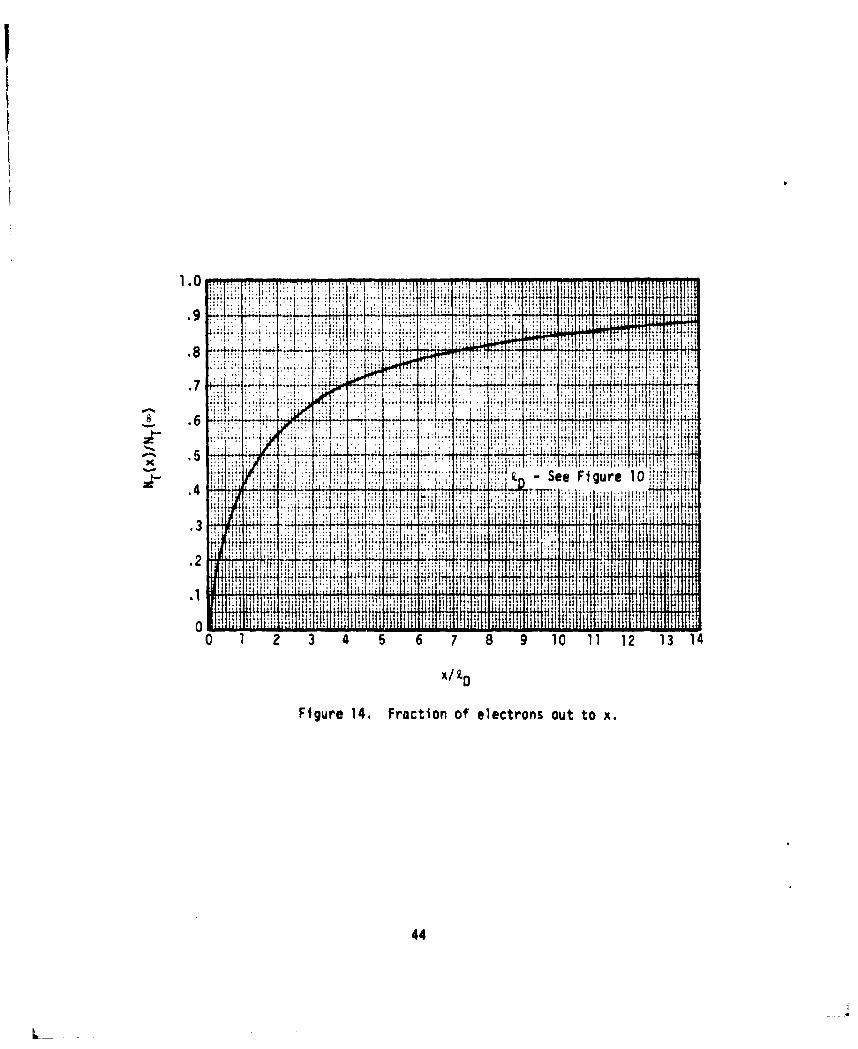
INTEGRATED NUMBER DENSITY

The integral of the number density out to x, NT(x), gives the total

number of electrons out to x,

x

NT(X) = JN(x) dx [electrons/cm] (18)

0

Gauss' law

aE- = 4 = -p 4rcN(x) , (19)

where c(>O) is the mngnitude of the clectron charge, 1 is the electric field,

and p = eN is the charge density, can be used to express NT(X) in terms of

E(x):

N.r(x) = ECiI (1 - (x) (20)r4-,re E(O)

Here, E(O) is the surface electric field, and E(O)/4,r is the surface charge

density. NT() = E(O)/47c. The fraction of electrons out to x, NT(X)/

NT(oJ, is shown in Figure 14.

It shows, for example, that one half of the electrons are contained

in the first 1.5 Debye lengths. The first Debye length contains about 41

percent of all the electrons. About 88 percent are contained in the first

11 I)ebye lengths.

The surface electric field itself, E(O) = Esurface' and the electric

field profile E(x)/E(O) are shown in the next two sections.

43

I

61 1.0

'V. ~ T.T . . ~. .. ee Fi ur.1..

IJ; 4ý 4.

it 460 r-Figure 14. Froct ~iono~eetonuu ox

... ... .. ...... .44..

SECTION 7

ELECTRIC FIELD AT SURFACE

We treat the electric field E(x) as a function of distance x from

.the surface also in two parts as we did the density. The surface electric

field

Esurface = E(x=O) , (21)

is given here. It also determines the surface charge density

Esurface (22)

and the total number of electrons

NT = surface (23)

to which Figure 14 was normalized.

The surface electric field [volts/meter] is shown in Figures 1Sa,

b, and c.

For example, a I keV blackbody incident on gold at 1 cal/cm/

nanosec produces a steady stat- field of about 7.4 10' volts/meter

(Figure iSb).

4 S

X-ray Flux, ;[a/m2/nnUe

101

0 00

10o 10

24

4 46

UX-ray Flux, $(cal/cm 2/nanosecJ

10 Z1

ITTT

4J

10 10

4. 4-8I

* LAJ ~10' wo

X-ayF~~ $ca/cZnao3c

Fiur INb SufcUlcrcfl o od

Numersoncuresarebakoytmeaue nky

V1 547

X-ray Flux. O4ca1/cm /naoflsecj

-1-141

4 ..

10 1

X-ray Flux, $(ca1/cm2/nanosec;j

Figure 15c. Surface electric field for Silicon Dioxide.


48

/

SS A

SECTION 8

ELECTRIC FIELD PROFILE

The electric field as a function of distance from the surface,

normalized to its surface value, E(x)/E surface, is shown in Figure 16.

As Equation 20 shows, this is one minus the total number of

electrons. It drops to l/e of its surface value in about 2.8 Debye lengths.

Together with the surface field from Figures ISa, b, or c, and the

Debye length from Figures 10a, b, or c, Figure 16 will give the electric

field at any distance from the surface in steady state.

49

S• /

7 -See Figure 10

:2!;H

U LL i'LL" 'L II'l--1 !I

Figure 16. Normalized electric field profile,

50

L

SECTION 9

PLASMA FREQUENCY AT SURFACE

If N is the local electron number density (cm3), the local plasma

frequency is defined asIV= -- N [radians/sec] (24)

We work instead with the frequency

p 27T

/_ Hz . (25)

We use the surface value of N, Equation 16, to obtain the surface plasma

frequency

elec • cal 1/2

fp a 1.746 X 1 4O ( lcal t cmanls). Hz (26)V4E I(keV)

This is shown in Figures 17a, b, and c.

For example an 8 keV blackbody on silicon dioxide at 10- cal/cm2 /

ns produces a surface plasma frequency of 9 x 1 Hz.

"The local plasma frequency at a distance from the surface drops off

as the square root of the number density, that is, as the square root of the

ordinate in Figures 12 or 13.51

/ •.

X-ray Flux, k~cal/cm 2/nanosec]

10 o'3102 10'l 1 - 101 1o2

108 100

10

10 1

25

3 ;7- d

Lwoo

X~-ray Flux, ýfcal/cn. /nanosec]

10

X-ra FAl [clc 2 naisc

53

X-ray Flux, ý[cal/cm 2/nanosec1

10 1

10 1

X-ra + lx ~a/c 2 nns

Fiur lc Srac p~rn reuec fr iicn ixie

Numbrs n crvesareblakbod teperture ink06

54

SECTION 10

DIPOLE MOMENT PER UNIT AREA

In Gaussian cgs units, the electric dipole moment of the layer

contributed by all electrons out to x is

xfP(x) = fxo(x) dx esu-cm/cm- (27)

0

Reference 1 shows this to be proportional to a universal dimensionless.function, .9(x/Z ) ), of x/2.D

1W(x) : e "(x/;[) esu/cm , (2)

where :1 (ergs) is the electron exponentiation energy w.hich was given in

kex in Table 2. If F1 is written in kcV, and l 1(x) in .IKS units, Equation

2S becomes

Coulombsl(x) = S.S54 0 E- I(keV) iP(x/)) meter (29)

Hence the quantity

r Coulombs0I (ke, ) L mter-keV3)

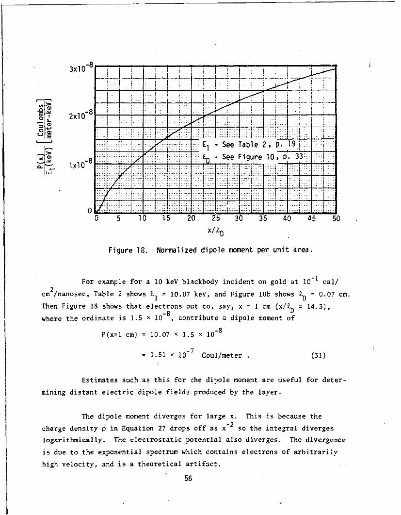
is a universal function of x/W. It is shown plotted in Figure 18.

To use Figure 18 for a certain blackbodv spectrum on a particular

material, first obtain EI- from Table 2, and the l)ebye length from Figure

1Oa, b, or c. Then to obtain the dipole moment out to x, multiply EI(keV)

by the ordinate in Figure 1. at the correct value of x/Zý.

55

-83xl 0 ...

I0 4J L 1

* 1 __ i 1[ 4

it " _ ..._

.1F - See Table 2, P. l10..

- ,.:>: :2: - See Figure 10, p. 33:-K

S....... . . . . . . . . . . ,. , -_i~ i

0 5 1 0 15 20 2b 30 35 40 45 50

Figure 18. Normalized dipole moment per unit area.

For example for a 10 keV blackbody incident on gold at 101I cal/2

cm /nanosec, Table 2 shows E1 = 10.07 keV, and Figure l0b shows 9.. = 0.07 cm.

Then Figure 18 shows that electrons out to, say, x = 1 cm (x/9.D = 14.3),

-8 D

where the ordinate is 1.5 x 10-8, contribute a dipole moment of

P(x=l cm) = 10.07 x 1.5 x 018

U-7

= 1.51 x 10 Coul/meter . (31)

Estimates such as this for the dipole moment are useful for deter-

mining distant electric dipole field3 produced by the layer.

The dipole moment diverges for large x. This is because the

charge density p in Equation 27 drops off as x -2 so the integral diverges

logaritemically. The electrostatic potential also diverges. The divergence

is due to the exponential spectrum which contains electrons of arbitrarily

high velocity, and is a theoretical artifact.

56

miigdsateeti ioe ilspoue ytelyr

Th ioemmn iegsfrlrex hsi eas h

II

To obtain a meaningful estimate for a real situation the following

procedure is suggested. At the time P(x) is desired, estimate the maximum

distance the most energetic electron traveling at less than the speed of

light could have gone. Determine P at this distance from Figure 18. Since

P increases slowly with distance, remaining of order a few times 10"a

Coulombs/meter for many I)cbye lengths, the exact distance x is not too

critical for rough estimates.

To convert P(x) to esu, use

I Coulomb ,3 1 0 7 e.umeter cm

57

BEST AVAILABLE COPY

SECTION 11

EXAMPLE

We discuss an example here to illustrate the use of all graphs.

We consider as a. example a S ke\' blacuhody s5wctrum incident on

aAhjinum with a time history a- shown in Figure 19, antl a fluenc, of I

eal/c'. This information, the incident spectrum, the target material. the

time history. and t'he fluence, we asuin•e given.

Irrespective of the time historyv and fIuence, rahbl I (or Figure I)

shows the hackscattered electron yield to he

iY .elctrun.sY * 2.$7 • J •'calorie (32)

Figure 5 shows. the approximate electron energy spectrum (for electron% of

energy greater than I kv\'. and i'ahle 2 shou- Chat the spectrum is nearly

exponential with exponent iat ion energy.

I. 1a -4.7' keV . 433)

The emission angular spectrum (per steradianl is approximately propoirtional

to coA, where -1 is the emissiun angle mcasured from the normal.

To estimate the time t after which we may use -tteadcy state theory

(and therefore all the graphs in this revtort,, we need at early times.

This is ohtained from Figure 09.

52

.8----

.6

.2 't2

0 10 20 30

Time (ns)

Figure 19. X-ray time history for Illustrative example.

59

o00

The maximum flux, 0mis determined from the fluence by

-f ; dt0

1*1 •*mt2

so that

a " a 6.67 x 10-2 cal/c,2 ns . (34)t 2

Then

m 1 - - 6.67 x 10 cal/cm 2ns (3S)ti

From Figure 8a we determine

t 0.9 ns . (36)

Thus after about one nanosec we can expect to be in quasi-steady state.

To see if we sensibly remain in instantdneous steady state, we must

have the flux change only slightly in the time t et, determined from Figure 9a

and an average $ of, say, *m/ 2 • 3 x 10. 2 cal/rnm2 /ns. Figure 9a shows

tret a 0.28 ns . (37)

During these times, Figure 19 shows the flux does change only slightly, so

we may expect sensible estimates from all remaining graphs.

The Debye length, Figure 10a, shortens in time as * increases, and

then lengthens again as $ decreases after its peak. Its smallest value is

when • ' Equation 34, for which Figure 10a shows

60

.. /4

mD,inimum 9.5 x 1-2 (38)

Th.e surface number density increases with * to a maximum of

Nfae,max 3 X 1011 elec/cm3 (39)

when . M , as shown by Figure Ila.

The number density profile is shown in Figure 12 or 13, and the

fractional integrated number in Figure 14. Figure 14 shows 75 percent of

the electrons inside 5.2 Debye lengths, or within about 0.5 cm at time

t 10 ns.

T?.e surface field increases as the square root of • to a maximum of

E = 4 x 10 v/m, (40)max

at 10 ns, as read from Figure 1Sa.

The electric field profile is shown in Figure ib.

The surface plasma frequency increases as the square root of the

flux reaching a maximum at 10 ns of

f xa 5 X 09 HN, (41);, ,max

as determine,' from Figure l7a.

The dipole moment out to 50 Debye lengths (v 4.8 cm using the

minimum Z, Equation 38) is shown in Figure 18 to be about

P % El(keV) x 3 x 10.8

- 1.4 - 10.7 Coulombs/meter , (42)

which is ahout 4.3 esu/cm.

61

BEST AVAILABLE COPY

REFERENCES

1. Carton, Neal J., and C. L. Longmire, On the Structure of the Steadyv-State, Space-Charge-Limited Boundary Layer in One Dimension, MissionResearch Corporation, MRC-R-240, November 1975.

2. Dellin, T. A., and C. J. MacCallum, QUICKE2: A One-Dimensional Code forCalculating Bulk and Vacuum Emitted Photo-Compton Currents, SandiaLaboratories, SLL-74-0218, April 1974.

3. Higgins, D. F., X-ray Induced Photoelectric Currents, Mission ResearchCorporation, MRC-R-81, June 1973.

62

ad-aq27 958 chapacteristic steady-state electron emission properties ... · pdf...

Documents