Ad Hoc Teamwork by Learning Teammates’Task

Yi Xia

University of Nebraska Lincoln

2018-10-08

F. S. Melo and A. Sardinha, “Ad hoc teamwork by learningteammates’ task”, Autonomous Agents and Multi-Agent Systems,vol. 30, no. 2, pp. 175–219, 2016, ISSN: 1573-7454. DOI:10.1007/s10458-015-9280-x. [Online]. Available:https://doi.org/10.1007/s10458-015-9280-x

OutlineIntroduction

Ad Hoc TeamworkAd Hoc Agent

Tackling the Ad Hoc Teamwork ProblemK-player Fully Cooperative Matrix GameBounded Rationality

Ad Hoc Agent ModelingOnline Learning AgentE-commerce ScenarioPOMDP Agent

Empirical EvaluationMethodology for Empirical EvaluationPerformance on a Set of ExperimentsScalability of Proposed ApproachPOMDO Evaluation and Tradeoff

ConclusionsQ&A

Introduction

Ad Hoc TeamworkAd Hoc Agent From the LiteratureAd Hoc Agent From a Novel Perspective

Ad Hoc Teamwork

The ad hoc teamwork setting is a situation when anautonomous agent must collaborate with other teammateagents to accomplish a common goal without priorcoordination.

Prior related work includes:1. Multi-armed bandits problem with a teacher and a student. [2]2. Robot soccer pick up games. [3]3. Ad hoc teamwork for leading a flock. [4]4. Multi-agent collaboration with open environment. [5]5. Ad hoc teamwork in the pursuit domain. [6]

Ad Hoc Agent

A good "ad hoc team player" must be adept at: [7]1. Assessing the capabilities of other agents.2. Assessing the other agents’ knowledge states.3. Estimating the effects of its actions on the other agents.

Evaluation framework proposed by Barrett and Stone. [8]1. Team knowledge2. Environment knowledge3. Reactivity of teammates

Ad Hoc Agent

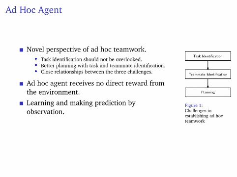
Novel perspective of ad hoc teamwork.� Task identification should not be overlooked.� Better planning with task and teammate identification.� Close relationships between the three challenges.

Ad hoc agent receives no direct reward fromthe environment.Learning and making prediction byobservation.

Figure 1:Challenges inestablishing ad hocteamwork

Tackling the Ad Hoc Teamwork Problem

K-player Fully Cooperative Matrix GameBounded Rationality

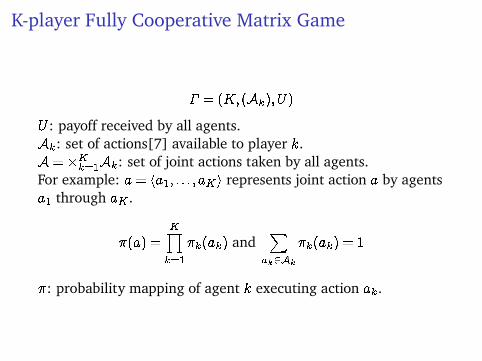
K-player Fully Cooperative Matrix Game

� = (K;(Ak);U)

U : payoff received by all agents.Ak: set of actions[7] available to player k.A=�K

k=1Ak: set of joint actions taken by all agents.For example: a= ha1; : : : ;aKi represents joint action a by agentsa1 through aK .

�(a) =KYk=1

�k(ak) andX

ak2Ak

�k(ak) = 1

�: probability mapping of agent k executing action ak.

K-player Fully Cooperative Matrix Game

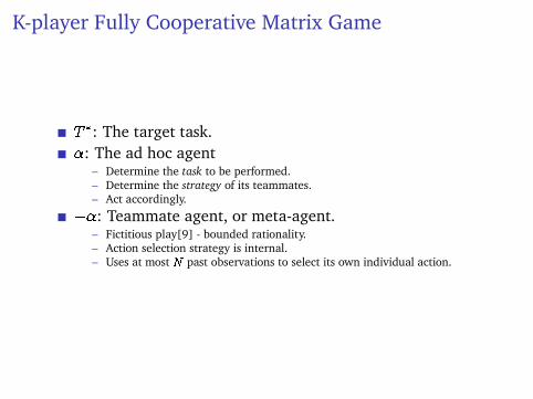
T �: The target task.�: The ad hoc agent

– Determine the task to be performed.– Determine the strategy of its teammates.– Act accordingly.

��: Teammate agent, or meta-agent.– Fictitious play[9] - bounded rationality.– Action selection strategy is internal.– Uses at most N past observations to select its own individual action.

Bounded Rationality

Let V (h1:n;a��) =1

N

N�1Xt=0

UT �(ha�(n� t);a��i) then,

���(h1:n;a���)> 0 only if a��� 2 argmaxa�� V (h1:n;a��)

– h1:n = fa(1); : : : ;a(n)g denotes a specific instance of historyH(n);n�N , where H(n) = fA(t); t= 1; : : : ;ng.

– ���(h1:n;a���) = P [Ak(n+1) = ak j a(n); : : : ;a(n�N +1)] :

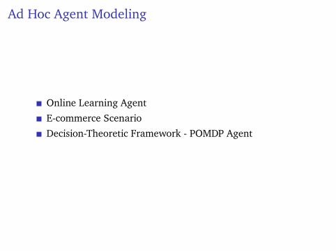
Ad Hoc Agent Modeling

Online Learning AgentE-commerce ScenarioDecision-Theoretic Framework - POMDP Agent

Online Learning AgentRecall that:

V k� (h1:n;ak) =

1

N

N�1Xt=0

U� (hak;a�k(n� t)i); k = �;��:

We can define the set of maximizing actions as:

Ak� (h1:n) = argmaxak2Ak

V k� (h1:n)

For best scenarios we define expert as a mappingE� :H�A! [0;1] such that:

E� (h1:n;a) = E�� (h1:n;a�)E

��� (h1:n;a��)

More precisely:

Ek� (h1:n;ak) =

(1

jAk� (h1:n)j

if ak 2 Ak� (h1:n)

0 otherwise; k = �;��

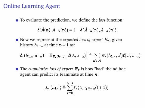
Online Learning Agent

To evaluate the prediction, we define the loss function:

`(A(n);A��(n)) = 1� �(A��(n);A��(n))

Now we represent the expected loss of expert E� , givenhistory h1:n, at time n+1 as:

`� (h1:n;a��) = EE� (h1:n)h`(A;a��)

i,Xa02A

E� (h1:n;a0)`(a0;a��)

The cumulative loss of expert E� is how "bad" the ad hocagent can predict its teammate at time n:

L� (h1:n),n�1Xt=0

`� (h1:t;a��(t+1))

Online Learning Agent

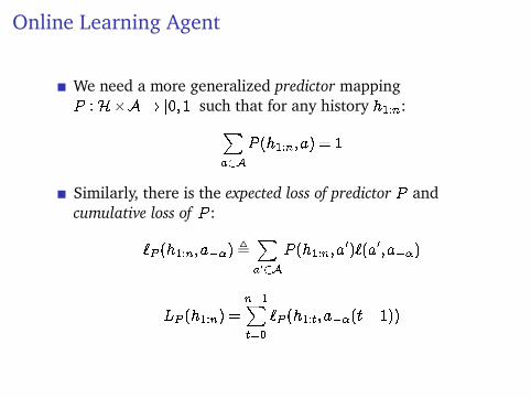
We need a more generalized predictor mappingP :H�A! [0;1] such that for any history h1:n:X

a2A

P (h1:n;a) = 1

Similarly, there is the expected loss of predictor P andcumulative loss of P :

`P (h1:n;a��),Xa02A

P (h1:n;a0)`(a0;a��)

LP (h1:n) =n�1Xt=0

`P (h1:t;a��(t+1))

Online Learning Agent

Determining a predictor that minimizes the expected regret:

Rn(P;E) = E [LP (h1:n)�L� (h1:n)]

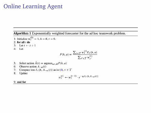
Choice of predictor P : exponentially weighted averagepredictor

P (h1:n; a),

P�2T e

� nL� (h1:n)E� (h1:n; a)P�2T e

� nL� (h1:n)

Online Learning Agent

E-commerce Scenario

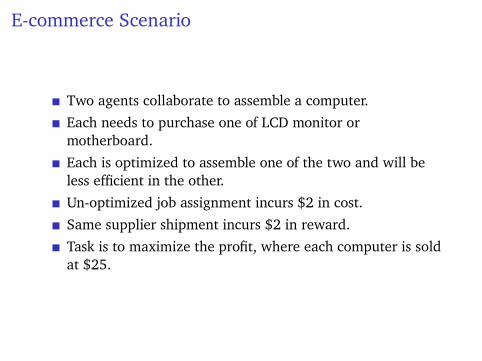
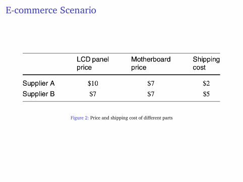
Two agents collaborate to assemble a computer.Each needs to purchase one of LCD monitor ormotherboard.Each is optimized to assemble one of the two and will beless efficient in the other.Un-optimized job assignment incurs $2 in cost.Same supplier shipment incurs $2 in reward.Task is to maximize the profit, where each computer is soldat $25.

E-commerce Scenario

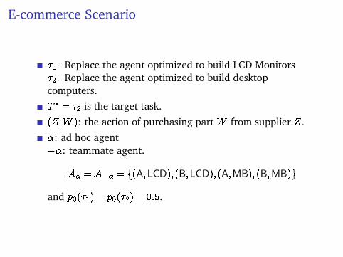
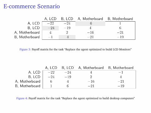
�1 : Replace the agent optimized to build LCD Monitors�2 : Replace the agent optimized to build desktopcomputers.T � = �2 is the target task.(Z;W ): the action of purchasing partW from supplier Z.�: ad hoc agent��: teammate agent.

A� =A�� =�(A;LCD);(B;LCD);(A;MB);(B;MB)

and p0(�1) = p0(�2) = 0:5.

E-commerce Scenario

Figure 2: Price and shipping cost of different parts

E-commerce Scenario

Figure 3: Payoff matrix for the task “Replace the agent optimized to build LCD Monitors”

Figure 4: Payoff matrix for the task “Replace the agent optimized to build desktop computers”

E-commerce Scenario

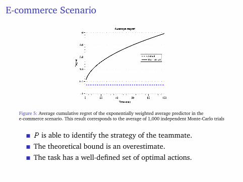
Figure 5: Average cumulative regret of the exponentially weighted average predictor in thee-commerce scenario. This result corresponds to the average of 1,000 independent Monte-Carlo trials

P is able to identify the strategy of the teammate.The theoretical bound is an overestimate.The task has a well-defined set of optimal actions.

Online Learning Agent Evaluation

What have we missed from the online learning agent model?

Online Learning Agent Evaluation

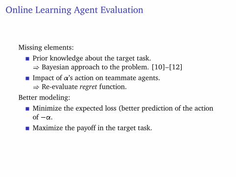
Missing elements:Prior knowledge about the target task.) Bayesian approach to the problem. [10]–[12]Impact of �’s action on teammate agents.) Re-evaluate regret function.

Better modeling:Minimize the expected loss (better prediction of the actionof ��.Maximize the payoff in the target task.

Decision-Theoretic Framework

T � is considered as an unobserved random variable.The ad hoc agent keep a distribution pn over the space ofpossible tasks at each time n.

pn(� ) = P [T � = � jH(n�1)] ;8� 2 T

pn(� ) is referred to as the belief of the agent � at time step nrelated to what the target task is.

POMDP Agent Modeling[13]

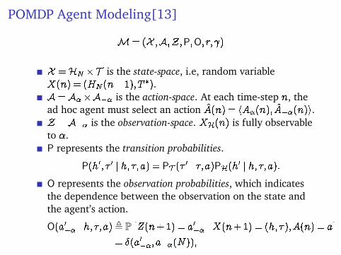
M= (X ;A;Z;P;O;r; )

X =HN �T is the state-space, i.e, random variableX(n) = (HN (n�1);T �).A=A��A�� is the action-space. At each time-step n, thead hoc agent must select an action A(n) = hA�(n); A��(n)i.Z =A�� is the observation-space. XH(n) is fully observableto �.P represents the transition probabilities.

P(h0; � 0 j h;�;a) = PT (� 0 j �;a)PH(h0 j h;�;a):O represents the observation probabilities, which indicatesthe dependence between the observation on the state andthe agent’s action.

O(a0�� j h;�;a), P�Z(n+1) = a0�� jX(n+1) = (h;� );A(n) = a

�= �(a0��;a��(N));

POMDP Agent Modeling

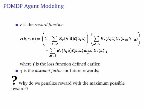
r is the reward function

r(h;�;a) =

0@1�

Xa2A

E� (h; a)`(a;a)

1A0@Xa2A

E� (h; a)U� (a�; a��)

1A

�Xa2A

E� (h; a)`(a;a)maxajU� (a)j ;

where ` is the loss function defined earlier. is the discount factor for future rewards.

?Why do we penalize reward with the maximum possiblerewards?

POMDP Agent Modeling

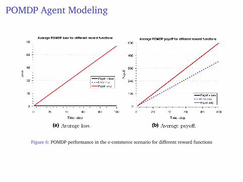
Figure 6: POMDP performance in the e-commerce scenario for different reward functions

Empirical Evaluation

Methodology for Empirical EvaluationPerformance on a Set of ExperimentsScalability of Proposed ApproachPOMDO Evaluation and Tradeoff

Methodology

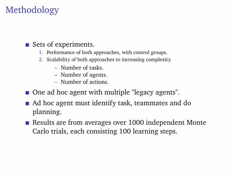
Sets of experiments.1. Performance of both approaches, with control groups.2. Scalability of both approaches to increasing complexity.

– Number of tasks.– Number of agents.– Number of actions.

One ad hoc agent with multiple "legacy agents".Ad hoc agent must identify task, teammates and doplanning.Results are from averages over 1000 independent MonteCarlo trials, each consisting 100 learning steps.

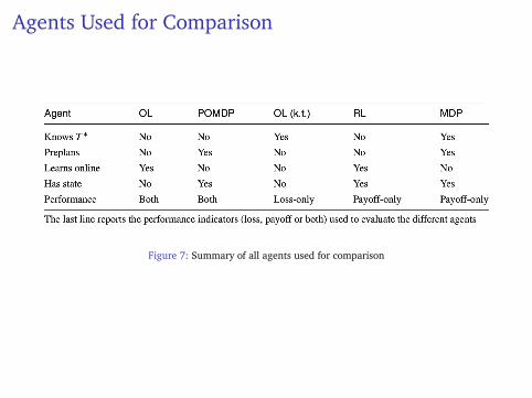
Agents Used for Comparison

Figure 7: Summary of all agents used for comparison

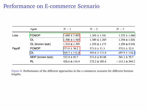
Performance on E-commerce Scenario

Figure 8: Performance of the different approaches in the e-commerce scenario for different horizonlengths.

Performance on E-commerce Scenario

Figure 9: Average discounted payoff of the different approaches in the e-commerce scenario for ahorizon H = 3.

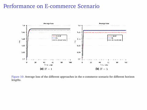
Performance on E-commerce Scenario

Figure 10: Average loss of the different approaches in the e-commerce scenario for different horizonlengths.

Performance on E-commerce Scenario

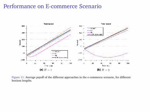
Figure 11: Average payoff of the different approaches in the e-commerce scenario, for differenthorizon lengths.

Scalability on Number of Tasks

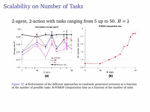
2-agent, 2-action with tasks ranging from 5 up to 50. H = 2

Figure 12: a Performance of the different approaches in randomly generated scenarios as a functionof the number of possible tasks. b POMDP computation time as a function of the number of tasks

Scalability on Number of Actions

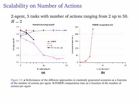
2-agent, 5 tasks with number of actions ranging from 2 up to 50.H = 2

Figure 13: a Performance of the different approaches in randomly generated scenarios as a functionof the number of actions per agent. b POMDP computation time as a function of the number ofactions per agent

Scalability on Number of Agents

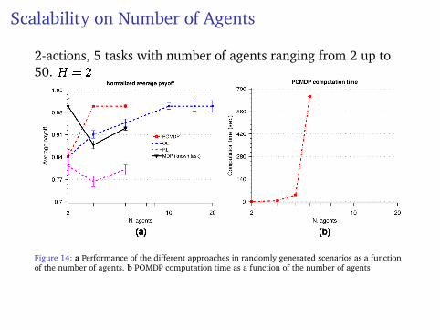
2-actions, 5 tasks with number of agents ranging from 2 up to50. H = 2

Figure 14: a Performance of the different approaches in randomly generated scenarios as a functionof the number of agents. b POMDP computation time as a function of the number of agents

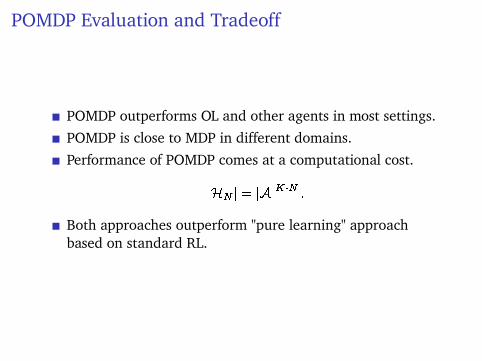
POMDP Evaluation and Tradeoff

POMDP outperforms OL and other agents in most settings.POMDP is close to MDP in different domains.Performance of POMDP comes at a computational cost.

jHN j= jAjK�N :

Both approaches outperform "pure learning" approachbased on standard RL.

Paper Conclusions

– Novel perspective of the ad hoc teamwork problem, focusingon task and teammate identification for better planning.

– Sequential decision formalization of the ad hoc teamworkproblem.

– Two approaches for ad hoc agent modeling.– Bounded rationality for both proposed approaches.– Performance comes at a cost.

My Conclusions

– Real-life scenarios involve large action space, POMDP mightnot be optimal strategy.

– Scalability issue with infinite memory on the horizon.– History component is simplified to the most recent actions only.– Real life humans have way more memories to make decisions on actions.

– Pre-processing of action space to better suit POMDPcomputation?

My Conclusions

– How does the agents perform in an open environment?– Agent openness and task openness essentially leads to dynamic action

space.– POMDP could perform well since it has a faster "start-up" speed.

– Bounded rationality relies heavily on "no mistake" agents.– Online learning will not perform well if the actions are noisy or certain

agents start to behave "crazy".– In other settings when risk assessment needs to be considered, will both

approaches will be applicable?

Thank you!Q & A

Reference I[1] F. S. Melo and A. Sardinha, “Ad hoc teamwork by learning teammates’ task”, Autonomous

Agents and Multi-Agent Systems, vol. 30, no. 2, pp. 175–219, 2016, ISSN: 1573-7454. DOI:10.1007/s10458-015-9280-x. [Online]. Available:https://doi.org/10.1007/s10458-015-9280-x.

[2] S. Barrett and P. Stone, “Ad hoc teamwork modeled with multi-armed bandits: An extensionto discounted infinite rewards”, in Proceedings of 2011 AAMAS Workshop on Adaptive andLearning Agents, 2011, pp. 9–14.

[3] M. Bowling and P. McCracken, “Coordination and adaptation in impromptu teams”, inProceedings of the 20th National Conference on Artificial Intelligence - Volume 1, ser. AAAI’05,Pittsburgh, Pennsylvania: AAAI Press, 2005, pp. 53–58, ISBN: 1-57735-236-x. [Online].Available: http://dl.acm.org/citation.cfm?id=1619332.1619343.

[4] K. Genter, N. Agmon, and P. Stone, “Ad hoc teamwork for leading a flock”, in Proceedings ofthe 2013 International Conference on Autonomous Agents and Multi-agent Systems, ser. AAMAS’13, St. Paul, MN, USA: International Foundation for Autonomous Agents and MultiagentSystems, 2013, pp. 531–538, ISBN: 978-1-4503-1993-5. [Online]. Available:http://dl.acm.org/citation.cfm?id=2484920.2485005.

[5] J. Jumadinova, P. Dasgupta, and L. Soh, “Strategic capability-learning for improvedmulti-agent collaboration in ad-hoc environments”, in 2012 IEEE/WIC/ACM InternationalConferences on Web Intelligence and Intelligent Agent Technology, vol. 2, 2012, pp. 287–292.DOI: 10.1109/WI-IAT.2012.57.

[6] S. Barrett, P. Stone, and S. Kraus, “Empirical evaluation of ad hoc teamwork in the pursuitdomain”, Autonomous Agents and Multiagent Systems (AAMAS), no. May, pp. 567–574, 2011.[Online]. Available: http://dl.acm.org/citation.cfm?id=2031678.2031698.

Reference II[7] P. Stone, G. A. Kaminka, S. Kraus, and J. S. Rosenschein, “Ad Hoc Autonomous Agent Teams :

Collaboration without Pre-Coordination”, Twenty-Fourth AAAI Conference on ArtificialIntelligence, no. July, pp. 1504–1509, 2010.

[8] S. Barrett and P. Stone, “An analysis framework for ad hoc teamwork tasks”, in Proceedings ofthe 11th International Conference on Autonomous Agents and Multiagent Systems - Volume 1,ser. AAMAS ’12, Valencia, Spain: International Foundation for Autonomous Agents andMultiagent Systems, 2012, pp. 357–364, ISBN: 0-9817381-1-7, 978-0-9817381-1-6.[Online]. Available: http://dl.acm.org/citation.cfm?id=2343576.2343627.

[9] D. Fudenberg, F. Drew, D. K. Levine, and D. K. Levine, The theory of learning in games. MITpress, 1998, vol. 2.

[10] E. Kaufmann, O. Cappé, and A. Garivier, “On bayesian upper confidence bounds for banditproblems”, in Artificial Intelligence and Statistics, 2012, pp. 592–600.

[11] J. C. Gittins, “Bandit processes and dynamic allocation indices”, Journal of the RoyalStatistical Society. Series B (Methodological), pp. 148–177, 1979.

[12] E. Kaufmann, N. Korda, and R. Munos, “Thompson sampling: An asymptotically optimalfinite-time analysis”, in International Conference on Algorithmic Learning Theory, Springer,2012, pp. 199–213.

[13] L. P. Kaelbling, M. L. Littman, and A. R. Cassandra, “Planning and acting in partiallyobservable stochastic domains”, Artif. Intell., vol. 101, no. 1-2, pp. 99–134, May 1998,ISSN: 0004-3702. DOI: 10.1016/S0004-3702(98)00023-X. [Online]. Available:http://dx.doi.org/10.1016/S0004-3702(98)00023-X.

[14] N. Cesa-Bianchi and G. Lugosi, Prediction, learning, and games. Cambridge university press,2006.

Reference III[15] S. Barrett, P. Stone, S. Kraus, and A. Rosenfeld, “Teamwork with limited knowledge of

teammates.”, in AAAI, 2013.

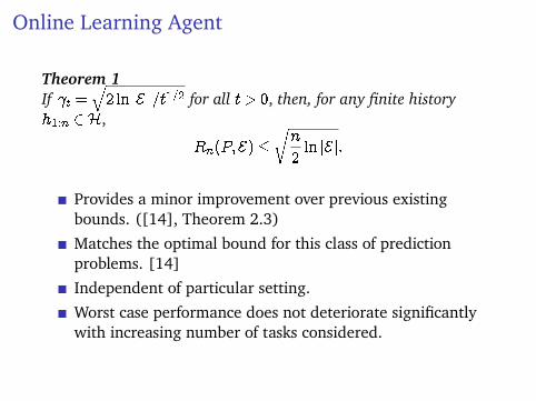
Online Learning Agent

Theorem 1If t =

q2ln jEj=t1=2 for all t > 0, then, for any finite history

h1:n 2H,

Rn(P;E)�

rn

2ln jEj:

Provides a minor improvement over previous existingbounds. ([14], Theorem 2.3)Matches the optimal bound for this class of predictionproblems. [14]Independent of particular setting.Worst case performance does not deteriorate significantlywith increasing number of tasks considered.

POMDP Agent

Theorem 2The POMDP-based approach to the ad hoc teamwork problem isa no-regret approach, i.e.,

limn!1

1

nRn(P;E) = 0:

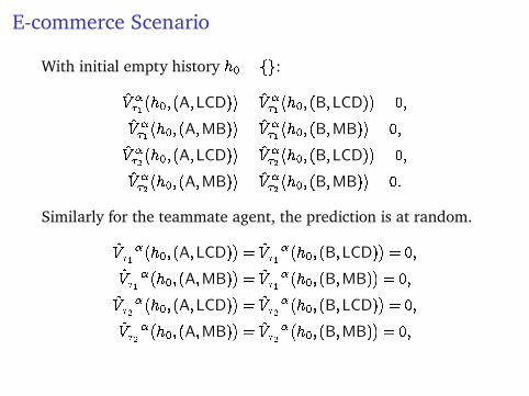
E-commerce Scenario

With initial empty history h0 = fg:

V ��1

�h0;(A;LCD)

�= V �

�1

�h0;(B;LCD)

�= 0;

V ��1

�h0;(A;MB)

�= V �

�1

�h0;(B;MB)

�= 0;

V ��2

�h0;(A;LCD)

�= V �

�2

�h0;(B;LCD)

�= 0;

V ��2

�h0;(A;MB)

�= V �

�2

�h0;(B;MB)

�= 0:

Similarly for the teammate agent, the prediction is at random.

V ���1

�h0;(A;LCD)

�= V ��

�1

�h0;(B;LCD)

�= 0;

V ���1

�h0;(A;MB)

�= V ��

�1

�h0;(B;MB)

�= 0;

V ���2

�h0;(A;LCD)

�= V ��

�2

�h0;(B;LCD)

�= 0;

V ���2

�h0;(A;MB)

�= V ��

�2

�h0;(B;MB)

�= 0;

E-commerce Scenario

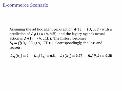
Assuming the ad hoc agent picks action A1(1) = (B;LCD) with aprediction of A2(1) = (A;MB), and the legacy agent’s actualaction is A2(1) = (A;LCD). The history becomesh1 = fh(B;LCD);(A;LCD)ig. Correspondingly, the loss andregrets:

L�1(h1) = 1; L�2(h1) = 0:5; LP (h1) = 0:75; R0(P;E) = 0:25

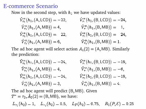
E-commerce ScenarioNow in the second step, with h1 we have updated values:

V ��1

�h1;(A;LCD)

�=�22;

V ��1

�h1;(A;MB)

�= 4;

V ��2

�h1;(A;LCD)

�=�22;

V ��2

�h1;(A;MB)

�= 6;

V ��1

�h1;(B;LCD)

�=�24;

V ��1

�h1;(B;MB)

�=�1;

V ��2

�h1;(B;LCD)

�=�24;

V ��2

�h1;(B;MB)

�= 1:

The ad hoc agent will select action A1(2) = (A;MB). Similarlythe prediction:

V ��1

�h1;(A;LCD)

�=�24;

V ��1

�h1;(A;MB)

�= 4;

V ��2

�h1;(A;LCD)

�=�24;

V ��2

�h1;(A;MB)

�= 3;

V ��1

�h1;(B;LCD)

�=�19;

V ��1

�h1;(B;MB)

�=�6;

V ��2

�h1;(B;LCD)

�=�19;

V ��2

�h1;(B;MB)

�= 4:

The ad hoc agent will predict (B;MB). GivenT � = �2; A2(2) = (B;MB), we have:L�1(h2) = 1; L�2(h2) = 0:5; LP (h2) = 0:75; R1(P;E) = 0:25

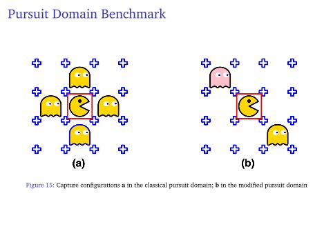
Pursuit Domain Benchmark

Figure 15: Capture configurations a in the classical pursuit domain; b in the modified pursuit domain

Pursuit Domain Benchmark

Figure 16: Comparative performance of the OL approach, the BSKR approach of Barrett et al. [15]and a standard RL agent in the pursuit domain. All results are averages over 1,000 independentMonte Carlo runs