Adaptive Isotopic Approximation of Nonsingular Curves:the Parametrizability and Nonlocal Isotopy Approach✩

Long Lin and Chee Yap

Courant Institute of Mathematical Sciences

New York University

251 Mercer Street

New York, NY 10012 USA

Abstract

We consider domain subdivision algorithms for computing isotopic approximations of nonsingular curvesrepresented implicitly by an equation f(X, Y ) = 0. Two algorithms in this area are from Snyder (1992)and Plantinga & Vegter (2004). We introduce a new algorithm that combines the advantages of these twoalgorithms: like Snyder, we use the parametrizability criterion for subdivision, and like Plantinga & Vegterwe exploit non-local isotopy. We further extend our algorithm in two important and practical directions:first, we allow subdivision cells to be rectangles with arbitrary but bounded aspect ratios. Second, we extendthe input domains to be regions R0 with arbitrary geometry and which might not be simply connected. Ouralgorithm halts as long as the curve has no singularities in the region, and intersects the boundary of R0

transversally. Our algorithm is practical and easy to implement exactly. We report some very encouragingexperimental results, showing that our algorithms can be much more efficient than the algorithms of Plantinga& Vegter and Snyder.

Key words: Meshing, Curve Approximation, Isotopy, Parametrizability, Subdivision Algorithms,Topological Correctness, Exact Algorithms.

✩This work is supported by NSF Grant CCF-0728977.Email address: {llin,yap}@cs.nyu.edu (Long Lin and Chee Yap)

Preprint submitted to Elsevier July 3, 2009

1. Introduction

Approximation of curves and surfaces is a basic problem in many areas such as simulation, computergraphics and geometric modeling. The approximate surface is often a triangulated surface, also known asa mesh. See the recent book [5] for an algorithmic perspective on meshing problems. We focus on curves,and in this case the “mesh” is just a (planar) straightline graph G (or PSLG, see [19]). Our problem is this:given a region R0 ⊆ R

2 of interest, an error bound ε > 0, a curve S implicitly represented by an equationf(X, Y ) = 0, to find a piecewise linear ε-approximation G of S ∩R0.

The correctness criteria for G has two parts: topological correctness and geometric accuracy.Geometric accuracy is typically taken to mean that the Hausdorff distance between G and S ∩R0 is at mostε. In recent years, the topological correctness is understood to mean that the approximate curve G shouldbe isotopic to S ∩R0; see [2] for further discussion of isotopy. Correspondingly, the meshing problem can be

solved in two stages: first we produce an output G̃ that is isotopic to S ∩R0. Subsequently, we refine G̃ intoa graph G with the requisite geometric accuracy. The first stage is more challenging and draws most of theattention.

There are three general approaches to meshing problems: algebraic, geometric or numeric. Algebraicapproaches are based on polynomial operations and algebraic number manipulation. Most algebraic al-gorithms can be reduced to the powerful tool of cylindrical algebraic decomposition (CAD) [1] but suchmethods are too inefficient, even in the plane. This has led to much interest in numerical algebraic meth-ods (e.g., [13]). But for special cases such as quadric surfaces [22] or cubic curves [11], efficient algebraicalgorithms have been devised. Geometric approaches exploit geometric properties such as Morse theory[25, 3] or Delaunay triangulations [10]. These geometric properties are encoded into the primitives used bythe algorithm. Typical primitives include the orientation predicates or ray shooting operations. Numericapproaches focus on approximation and numerical primitives such as function evaluation [14, 18]. Suchprimitives are usually embedded in simple global iterative schemes such as bisection. There is considerablework along this line in the interval arithmetic community (e.g., Martin et al [15]). These algorithms are oftencalled “curve tracing algorithms”. See Ratschek and Rokne [21] for references to curve tracing papers. Untilrecently, numeric approaches were shunned by computational geometers as lacking exactness or complexityanalysis. This is unfortunate as practitioners overwhelmingly favor numeric approaches for two simple rea-sons: they are efficient and easy to implement. Our overall goal is to address the above shortcomings ofnumerical approaches while retaining their advantages. Clearly, some algorithms are best viewed as hybridsof these approaches. All three approaches are exemplified in the survey [2].

As suggested above, geometric algorithms are usually described in an abstract computational model thatpostulates certain geometric primitives (i.e., operations or predicates). These primitives may be implementedeither by numerical or algebraic techniques; the algorithm itself is somewhat indifferent to this choice. Forthe meshing problem, a popular approach is based on sampling points on input surface [10, 4, 2]. Thegeometric primitive here is ray-shooting; it returns the first point (if it exists) that the ray intersects on theinput surface. For algebraic surfaces, this primitive reduces to a special case of real root isolation (namely,finding the smallest positive real root). The sampled points have algebraic number coordinates. In addition,the algorithms typically maintain a Delaunay triangulation of the sampled points, and thus would needorientation predicates on algebraic points. But exact implementation of these primitives requires expensiveand nontrivial algebraic number manipulations. This does not seem justified in meshing applications. Onthe other hand, if we use approximations for sample points, these may no longer lie on the surface. Thisgives rise to the well-known “implementation gap” concerns of computational geometry [26]: nonrobustness,degeneracies, approximation, etc. In contrast, the subdivision methods studied in this paper suffers nosuch implementation gaps. As subdivision methods are important to large communities of practitioners innumerical scientific computation, it behooves us to develop such methods into exact and quantifiable toolsfor geometric algorithms.

¶1. Recent Progress in Subdivision Algorithms. In this paper, we focus on algorithms based on domain1

subdivisions methods. Figure 1 illustrates the output of four such algorithms on the input curve f(X, Y ) =

1We use the term “domain subdivision” to refer to the subdivision of the underlying space R2 or R

3 in which the curve orsurface lives. Subdivision can also take place in parameter space, as in Bezier surfaces.

1

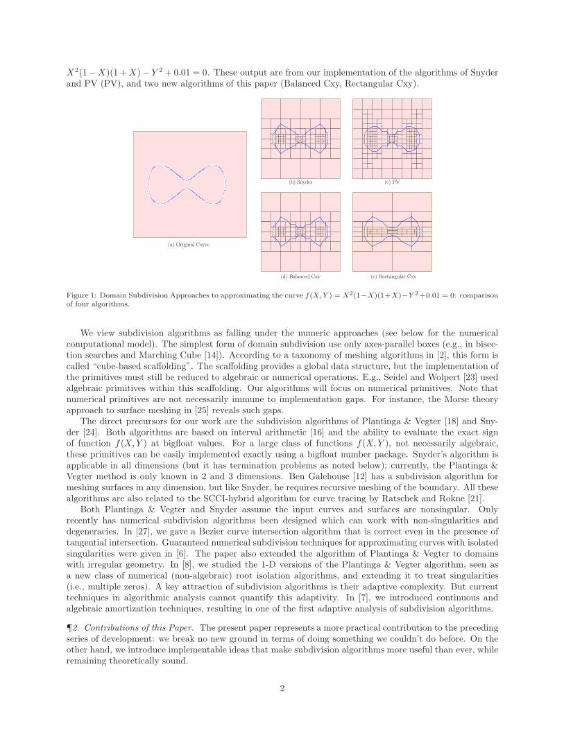
X2(1−X)(1 + X)− Y 2 + 0.01 = 0. These output are from our implementation of the algorithms of Snyderand PV (PV), and two new algorithms of this paper (Balanced Cxy, Rectangular Cxy).

(b) Snyder (c) PV

(e) Rectangular Cxy(d) Balanced Cxy

(a) Original Curve

Figure 1: Domain Subdivision Approaches to approximating the curve f(X, Y ) = X2(1−X)(1+X)−Y 2+0.01 = 0: comparisonof four algorithms.

We view subdivision algorithms as falling under the numeric approaches (see below for the numericalcomputational model). The simplest form of domain subdivision use only axes-parallel boxes (e.g., in bisec-tion searches and Marching Cube [14]). According to a taxonomy of meshing algorithms in [2], this form iscalled “cube-based scaffolding”. The scaffolding provides a global data structure, but the implementation ofthe primitives must still be reduced to algebraic or numerical operations. E.g., Seidel and Wolpert [23] usedalgebraic primitives within this scaffolding. Our algorithms will focus on numerical primitives. Note thatnumerical primitives are not necessarily immune to implementation gaps. For instance, the Morse theoryapproach to surface meshing in [25] reveals such gaps.

The direct precursors for our work are the subdivision algorithms of Plantinga & Vegter [18] and Sny-der [24]. Both algorithms are based on interval arithmetic [16] and the ability to evaluate the exact signof function f(X, Y ) at bigfloat values. For a large class of functions f(X, Y ), not necessarily algebraic,these primitives can be easily implemented exactly using a bigfloat number package. Snyder’s algorithm isapplicable in all dimensions (but it has termination problems as noted below); currently, the Plantinga &Vegter method is only known in 2 and 3 dimensions. Ben Galehouse [12] has a subdivision algorithm formeshing surfaces in any dimension, but like Snyder, he requires recursive meshing of the boundary. All thesealgorithms are also related to the SCCI-hybrid algorithm for curve tracing by Ratschek and Rokne [21].

Both Plantinga & Vegter and Snyder assume the input curves and surfaces are nonsingular. Onlyrecently has numerical subdivision algorithms been designed which can work with non-singularities anddegeneracies. In [27], we gave a Bezier curve intersection algorithm that is correct even in the presence oftangential intersection. Guaranteed numerical subdivision techniques for approximating curves with isolatedsingularities were given in [6]. The paper also extended the algorithm of Plantinga & Vegter to domainswith irregular geometry. In [8], we studied the 1-D versions of the Plantinga & Vegter algorithm, seen asa new class of numerical (non-algebraic) root isolation algorithms, and extending it to treat singularities(i.e., multiple zeros). A key attraction of subdivision algorithms is their adaptive complexity. But currenttechniques in algorithmic analysis cannot quantify this adaptivity. In [7], we introduced continuous andalgebraic amortization techniques, resulting in one of the first adaptive analysis of subdivision algorithms.

¶2. Contributions of this Paper. The present paper represents a more practical contribution to the precedingseries of development: we break no new ground in terms of doing something we couldn’t do before. On theother hand, we introduce implementable ideas that make subdivision algorithms more useful than ever, whileremaining theoretically sound.

2

Our main contribution is a new approach, and a corresponding new meshing algorithm, that combinesthe relative advantages of Snyder and Plantinga & Vegter: we retain the weaker Cxy-predicate of Snyder,but like Plantinga & Vegter, we do not require local isotopy. Our processing of each box is just as simple asin PV. However, achieving geometric accuracy is somewhat harder with the Cxy-predicate. We will addressthis issue separately.

In this paper, we give the first complete proof of the global isotopy of the Plantinga & Vegter method.Such a proof, being global, is more subtle than the correctness of Snyder’s parametrizability approach (whichis entirely local).

When meshing a curve that is almost horizontal in some neighborhood, it is very useful to allow boxesin that neighborhood to be elongated along the horizontal direction. Note that the PV algorithm limits theaspect ratios of boxes to be less than 2. So another contribution is to allow subdivision boxes with variablebut bounded aspect ratio. The aspect ratio of a box is the length of the longest side of a box over thatof its shortest side. This further improves the adaptivity of our method. Other practical improvementsinclude allowing domains of arbitrary geometry, as in [6]. Thus the input domains need not be connected orsimply-connected.

We have implemented our algorithms, and to perform comparisons, we have also implemented thePlantinga & Vegter and Snyder’s algorithms. We will provide experimental evidence showing that ournew approach can greatly speed up the previous algorithms. See Figure 1 for some impressions of our ap-proach: our Balanced Cxy Algorithm produce fewer boxes than Plantinga & Vegter, but unlike Snyder, weachieved this without having to isolating roots. The Rectangular Cxy Algorithm produces even fewer boxesthan Snyder’s Algorithm.

2. Overview of Subdivision Algorithms

To provide intuitions for our new results, we will recall the work of Snyder and Plantinga & Vegter. Inmost of our discussion, we fix a real curve

S := f−1(0) ={p ∈ R

2 : f(p) = 0}

. (1)

which is specified by a C1 function, f(X, Y ) : R2 → R. We assume interval arithmetic and interval versions

of functions such as f and its partial derivatives fx, fy.A box is given by B = I × J ⊆ R

2 where I, J are real intervals. Let m(I) and w(I) denote the midpointand width of I. For a box B = I × J , let wx(B) := w(I), mx(B) = m(I); similarly for wy(B), wy(B). Thenthe midpoint, width and diameter of B are (resp.) m(B) := (mx(B), my(B)), w(B) := min {wx(B), wy(B)}and d(B) := max {wx(B), wy(B)}. We name the four sides and corners of a box B by their compassdirections (north, south, east, west and NE, NW, SW, SE). We say B has uniform sign if the inputfunction f has the same sign at each of its four corners. If p, q ∈ R are the SW and NW corners of B, wemay denote B = [p, q]. A full-split of B is to subdivide B into four equal subboxes; a half-split subdividesB into two equal subboxes. There are two kinds of half-splits: horizontal and vertical. These subboxes arecalled the children of B. If the children of the full split of B are denoted B1, . . . , B4 (with Bi in the ithquadrant relative to m(B)), then the children in a horizontal (resp., vertical) half-split are B12, B34 (resp.,B14, B23), where Bij = Bi ∪Bj . We use the side/corner terminology for boxes, but reserve the edge/vertexterminology for the approximation straightline graphs G (or PSLG [19]).

¶3. Our Computational Model. To see why our algorithms are free of implementation gaps, we take acloser look at the computational model we need. Bigfloats or dyadic numbers is the set F = Z[1/2] = {m2n :m, n ∈ Z}. All numerical computations in our algorithms will be reduced to exact ring operations (±,×) andcomparisons on bigfloat numbers. Bigfloat number packages are efficient and widely available (e.g., GMP,LEDA or Core Library). More generally, F can be replaced by any “computational ring” [28] satisfying somebasic axioms to support exact real approximation.

We also use interval arithmetic [16] – the main tool being inclusion functions ([20]). An inclusion functionfor f(X, Y ) is a function f(I, J) = f(B) that takes input intervals and returns an interval that satisfiesthe inclusion property: f(B) = {f(x, y) : (x, y) ∈ B} ⊆ f(B). We call f a box function for f if, inaddition, it is point convergent, i.e., for any strictly decreasing sequence B0 ⊃ B1 ⊃ · · · of boxes thatconverges to a point p, we have f(Bi) → p as i → ∞. For our computational model, it is assumed that

3

the input arguments to f are dyadic boxes, and it returns a dyadic box. We also need box versions of thederivatives, fx, fy.

As in [6], we call f a PV function if f : R2 → R is C1, and there exist computable box functions

f, fx, fy and the sign of f at dyadic points p ∈ F2 is computable. It will be clear that the algorithms of

this paper can be easy to implement with no numerical errors when the input f are PV functions, and allnumerical inputs are dyadic. Therefore, nonrobustness issues are moot. See [6, 20] for additional information.

In contrast to our computational model, the standard model of numerical analysis only supports inexactarithmetic (up to unit round-off error). This leads to the implementation gap issues mentioned in theintroduction. Such a model is assumed Ratschek and Rokne, and even though they have the same basicapproach as this paper, they had to discuss rounding errors [21, §2.5]. Moreover, in their model, computingthe sign of f(X, Y ) at a point p = (x0, y0) is problematic.

¶4. Generic Subdivision Algorithm. The subdivision algorithms in this paper have a simple global structure.Each algorithm has a small number of steps called phases. Each phase takes an input queue Q and returnssome output data structure, Q′. Note that Q′ need not be a queue, but Q is always a queue of boxes. Eachphase is a while-loop that extracts a box B from Q, processes B, possibly re-inserting children of B backinto Q. The phase ends when Q is empty. If Q′ is a queue of boxes, it could be used as input for the nextphase. We next describe a generic algorithm with three phases: Subdivision, Refinement and Construction.

For the Subdivision Phase, the input Qin and output Qout are both queues holding boxes. The subdivisiondepends on two box predicates, Cin(B) and Cout(B). For each box B extracted from Qin, we first checkif Cout(B) holds. If so, B is discarded. Otherwise, if Cin(B) holds, then insert B into Qout. Otherwise,we full-split B and insert the children into Qin. Next, the Refinement Phase takes the output queue fromSubdivision, and further subdivide the boxes to satisfy additional criteria – these refined boxes are put inan output queue Qref . Strictly speaking, it should be possible to combine refinement with the subdivisionphase. Finally, the Construction Phase takes Qref as its input and produces an output structure G = (V, E)representing a planar straight line graph. As we process each box B in the input queue, we insert verticesand edges into V and E, respectively.

Generic Subdivision Algorithm

Input: Curve S given by f(X, Y ) = 0, box B0 ⊆ R2 and ε > 0

Output: Graph G = (V, E) as an isotopic ε-approximation of S ∩B0.0. Let Qin ← {B0} be a queue of boxes.1. Qout ← SUBDIV IDE(Qin)2. Qref ← REFINE(Qout)3. G← CONSTRUCT (Qref)

¶5. Example: Crude Marching Cube. Let us instantiate the generic algorithm just described, to produce acrude but still useful algorithm for “curve tracing” (cf. [15]). For the Subdivision Phase, we must specifytwo box predicates: let the Cout predicate be instantiated as

C0(B) : 0 /∈ f(B) (2)

If C0(B) holds, clearly the curve S does not pass through B, and B may be discarded. Let Cin predicatebe instantiated by Cε(B) which states that the sides of B have lengths less than some ε > 0. Thus, all theboxes in output Qout have width ≤ ε. The current Refinement Phase does nothing (so Qref = Qout). Forthe Construction Phase, we must specify how to process each box B ∈ Qref . The goal is to create vertices tobe inserted into V , and create edges (which are straightline segments joining pairs of vertices) to be insertedinto E. The output is a straightline graph G = (V, E).

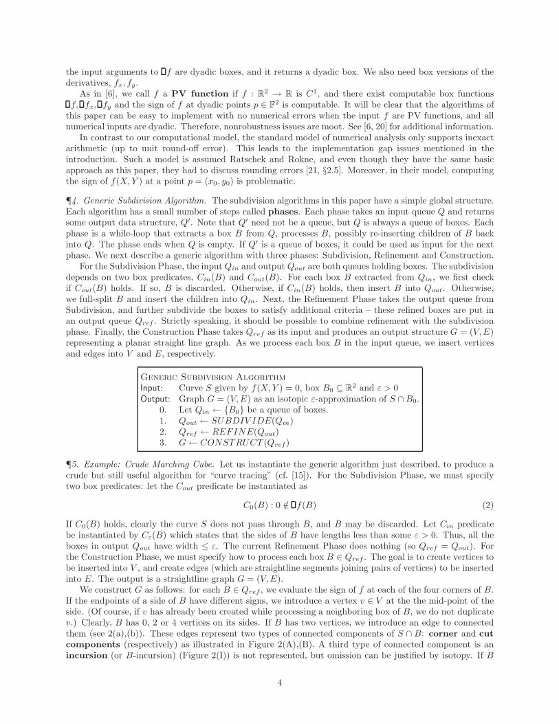
We construct G as follows: for each B ∈ Qref , we evaluate the sign of f at each of the four corners of B.If the endpoints of a side of B have different signs, we introduce a vertex v ∈ V at the the mid-point of theside. (Of course, if v has already been created while processing a neighboring box of B, we do not duplicatev.) Clearly, B has 0, 2 or 4 vertices on its sides. If B has two vertices, we introduce an edge to connectedthem (see 2(a),(b)). These edges represent two types of connected components of S ∩ B: corner and cutcomponents (respectively) as illustrated in Figure 2(A),(B). A third type of connected component is anincursion (or B-incursion) (Figure 2(I)) is not represented, but omission can be justified by isotopy. If B

4

−

(b)

+

+

Corner:

Vertex:

KEY:

(C)

−− +

+

+

++

+

(A)

+ −

(B)

+

+

+

+

− +

+

−

+

(a)

−

−

(d)

+

+−

+

−

−

(c)

Figure 2: Components Types: (A) corner, (B) cut, (C) incursion. Simple Connection Rules: (a,b) corner and cut edge; (c,d)double corner edges.

has 4 vertices, we introduce two pairs of non-intersecting edges to connect them (see Figure 2(c,d)); thereare two ways to do this, but we choose either one arbitrarily. In general, the corners of B may have a zerosign. But henceforth, we give them an arbitrary sign (say, positive). This can be justified by isotopy, as [18].

This completes our description of a crude Marching Cube algorithm. Other subdivision algorithms tobe discussed will be seen as refinements of this crude algorithm. The output graph G = (V, E) is anapproximation to S ∩B0, up to “ε resolution”. If ε is screen resolution, this is adequate for the purposes ofgraphical display. Martin et al [15] gave a comparative study of various numerical implementations of thebox predicates Cout, Cin.

¶6. Snyder’s Parametrizability Approach. Our crude Marching Cube makes no claims on topological cor-rectness. Until recently, no numerical subdivision algorithms can promise much better. In particular, theability to handle singularities is regarded as an open problem for numerical methods [2, p. 182]. But manypapers assume manifolds in order to avoid singularity. In the present paper, we only assume that the curve Shas no singularities in the region R0 of interest. More precisely, f2 + f2

x + f2y does not vanish at any point in

R0. Our main issue is to ensure isotopy in such a situation. In domain subdivision, two related approacheshave been introduced by Snyder [24] and Plantinga & Vegter [18]. In Snyder’s approach, the predicate Cin

is chosen to beCxy(B) : Cx(B) ∨ Cy(B) (3)

where Cx(B) is the predicate 0 /∈ fx(B), and similarly for Cy(B) with respect to fy. A curve S is said to beparametrizable in the x-direction (or, x-parametrizable) in a box B if each vertical line intersects S ∩Bat most once. Clearly, Cy(B) implies that S is x-parametrizable in B; this is illustrated in Figure 3. Duringthe Construction Phase, we isolate the intersections of S with the boundary ∂B of each box B ∈ Qref (thisamounts to root isolation). With sufficient root refinement, we would be able to correctly construct theisotopy type of S ∩B. Note that this isotopy type can be arbitrarily complex, as seen in Figure 3.

I7

−

+

−−

++

−

+

I5 I6I1 I2 I3 I4

Figure 3: The box components of a Cy-box

5

¶7. Plantinga & Vegter’s Small Normal Variation Approach. Unfortunately, Snyder’s algorithm (assumingthat the method is recursively applied to the boundary of B) may not terminate2 if the curve intersects ∂Btangentially [2, p. 195]. In view of this, the credit for the first complete subdivision algorithm to achieveisotopic approximation of nonsingular curves and surfaces belongs to Plantinga & Vegter [18]. In place ofCxy(B), the Plantinga & Vegter (or PV) algorithm uses a stronger predicate that we denote by C1(B):

C1(B) : 0 /∈ ( fx(B))2 + ( fy(B))2. (4)

It is called the “small normal variation” condition in [2]. To see that C1(B) implies Cxy(B), we can follow[18] by rewriting the condition as

0 /∈ 〈 ∇f(B), ∇f(B)〉where ∇f(p) := (fx(p), fy(p)) denotes the gradient at a point p, and f(B) := ( fx(B), fy(B)), and 〈·, ·〉 isjust scalar product of a vector. This shows that if p, q ∈ B, then 〈∇f(p),∇f(q)〉 > 0. Suppose some p ∈ Bhas a vertical gradient (there are two choices, up or down). Then no q ∈ B can have a horizontal gradient(there are two choices, left or right). We conclude that f−1(0) ∩ B is parameterizable in the x-direction.There is a symmetric argument in which the roles of horizontal and vertical directions are inter-changed.The PV algorithm has a remarkable nonlocal isotopy property:

It does not guarantee isotopy of the approximation G with the curve S within each box B ∈ Qref . (5)

We view this property favorably because local isotopy in each B is seen as an artifact of the subdivisionscheme, and could greatly increase the number of subdivisions. The non-termination of Snyder’s algorithmis precisely because it insists on local isotopy. The processing of C1-boxes is extremely simple as compared toSnyder’s approach. In fact, it is a slight extension of the connection rules in our crude Marching Cube above(see §15 Figure 7). This advantage shows up even more in 3-D, where Snyder’s algorithm must recursivelysolve the 2-D isotopy problem on the boundary of each subdivision box. On the negative side, C1(B) is astronger predicate than Cxy(B) and may cause more subdivisions than Cxy(B). In view of these tradeoffs,it is not immediately clear which approach is more efficient.

¶8. Quadtrees. Instead of queues, we prefer to work with a slightly more elaborate structure: a quadtree isa rooted tree T whose nodes u are associated with boxes B(u) and if u is an internal node then it either hasfour or two children whose associated boxes are obtained by full- or half-splitting B(u). Two nodes u, v aresaid to be adjacent (or neighbors) if the interiors of B(u) and B(v) are disjoint, but their boundary overlap.Overlapping means B(u) ∩ B(v) is a line segment, not just a point or empty. In order for T to representregions of fairly complex geometry, we assume that each leaf of T is tagged with a Boolean flag, “in” or“out”. So we may speak of the in-leaves or out-leaves of T . The associated boxes are called in-boxesor out-boxes. The quadtree T represents a region denoted R(T ) ⊆ R

2 which is just the union of all thein-boxes. Following [6], we call R(T ) a nice region. The notion of side/corner is relative to a box B.

A refinement step is an operation on a quadtree T in which we split any in-leaf u ∈ T , and taggingthe children as in or out. Note that we do not split out-leaves. Although the original tagging is arbitrary,subsequent tagging of new nodes created by refinement must follow a fixed rule, depending on some fixedpair of box predicates π = (πin, πout). We tag a node as “out” if it’s associated box B satisfies πout(B), elseit is “in”. If πin(B) holds but not πout(B), we say B is terminal. In this paper, πout is always the predicateC0 above; it ensures that out-boxes can safely be omitted in our approximation of the curve S. So we onlyfocus on πin.

To recap, our algorithm begins with a nice region R(T ) in which the tagging of nodes of T are arbitrarilyassigned. Subsequently, we refine T using the above rules for tagging new nodes. Thus, there are two typesof “out” leaves: original or C0, and two types of “in” leaves: terminal or non-terminal.

A refinement of T is obtained by a sequence of refinement steps. Note that if T ′ is a refinement ofT , then R(T ′) ⊆ R(T ). We are interested in three properties of quadtrees T , each obtained by successiverefinements:

2In meshing curves, one can handle this problem by some root isolation method that handle multiple roots, but the problemis more serious in meshing surfaces.

6

• SUBDIV IDEπin(T ) returns a quadtree that satisfies the pair π = (πin, C0) of box predicates, i.e.,

each out-box B is either originally tagged as “out” or else C0(B) holds, and each in-box must satisfyπin, but not C0.

• REGULARIZE(T ) returns a regular quadtree, i.e., any two adjacent in-boxes have the same depth.Thus,

REGULARIZE(T ) ≡ SUBDIV IDEπreg(T )

where πreg(B) ≡ all in-boxes adjacent to B have width≥ w(B). Note that this is more general thanPlantinga & Vegter’s notion of regularity which requires all the leaves to have the same depth, sincethe leaves of different connected components of R(T ) are allowed to have different depths.

• BALANCE(T ) returns a balanced quadtree, i.e., one where the depths of any two adjacent in-boxesdiffer by at most one. Thus,

BALANCE(T ) ≡ SUBDIV IDEπbal(T )

where πbal(B) ≡ all in-boxes adjacent to B have width≥ 12w(B).

A useful terminology is the notion of “segments” of a quadtree T . Roughly speaking, segments are theunits into which a side of a box is subdivided. There are two types of segments: a boundary segment eis a side of an in-box of T such that e ∈ ∂R(T ); an internal segment e has the form e = B ∩ B′ whereB, B′ are adjacent in-boxes of T . Thus each side of a box in T is divided into one or more segments. If Tis a regular quadtree, then each side of an in-box of T is also a segment; if T is a balanced quadtree, theneach side of an in-box of T is composed of either one or two segments. A boundary box is an in-box thathas a boundary segment as one of its sides.

For now, assume the above 3 subroutines use only full-splits; the general case where we also allow half-splits is treated in Section 7. Given a quadtree T , we assume a simple subroutine Q ← InBox(T ) thatreturns a queue Q containing all the in-boxes in T . Thus, the above 3 subroutines can be viewed as “phases”(see ¶4) whose input queues are InBox(T ). These subroutines are easily implemented by a simple while-loopas described earlier.

¶9. Perturbation. The correctness statements of geometric algorithms can be quite involved in the presenceof degeneracy. To avoid such complications, and in the spirit of exploiting nonlocal isotopy, we exploitperturbations of f . We call f̃ : R

2 → R a nice perturbation of f : R2 → R relative to T if

i) f̃−1(0) ∩ Interior(R(T )) ≈ f̃−1(0) ∩R(T ).ii) ∀ǫ > 0, ∃fǫ : R

2 → R such that (a) |f(q)− fǫ(q)| < ǫ for ∀q ∈ R2, and (b) f̃(p)fǫ(p) > 0, for any corner p

of T .

Lemma 1. For any given f and T , there exists an nice perturbation f̃ of f relative to T .

From now on, we assume f has been replaced by some nice perturbation (relative to some T ).

3. Regular Cxy Algorithm

In this paper, we will describe three increasingly sophisticated subdivision algorithms for curves, allbased on the Cxy predicate. These will be known as the Regular Cxy, Balanced Cxy and Rectangular CxyAlgorithms. For the first two algorithms, we only perform full-splits of boxes. We now present the first ofthese three algorithms.

Our initial goal is to replace the C1-predicate in the PV Algorithm by the parametrizability conditionof Snyder. As in Plantinga & Vegter [18], we first consider a simplified version in which we regularize thequadtree, i.e., reduce all adjacent in-boxes to the same depth. This is our Regular Cxy Algorithm. Oursimplified algorithm has this form:

7

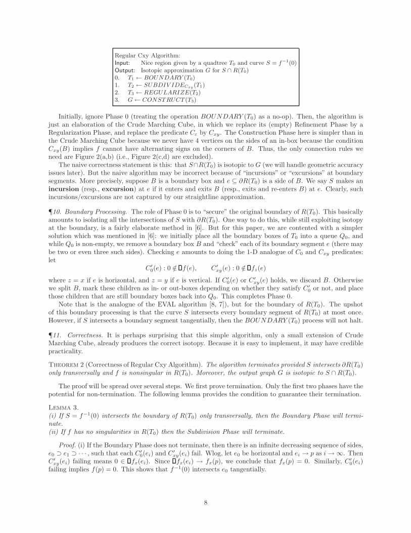
Regular Cxy Algorithm:Input: Nice region given by a quadtree T0 and curve S = f−1(0)Output: Isotopic approximation G for S ∩ R(T0)0. T1 ← BOUNDARY (T0)1. T2 ← SUBDIV IDECxy(T1)2. T3 ← REGULARIZE(T2)3. G← CONSTRUCT (T3)

Initially, ignore Phase 0 (treating the operation BOUNDARY (T0) as a no-op). Then, the algorithm isjust an elaboration of the Crude Marching Cube, in which we replace its (empty) Refinement Phase by aRegularization Phase, and replace the predicate Cε by Cxy. The Construction Phase here is simpler than inthe Crude Marching Cube because we never have 4 vertices on the sides of an in-box because the conditionCxy(B) implies f cannot have alternating signs on the corners of B. Thus, the only connection rules weneed are Figure 2(a,b) (i.e., Figure 2(c,d) are excluded).

The naive correctness statement is this: that S∩R(T0) is isotopic to G (we will handle geometric accuracyissues later). But the naive algorithm may be incorrect because of “incursions” or “excursions” at boundarysegments. More precisely, suppose B is a boundary box and e ⊆ ∂R(T0) is a side of B. We say S makes anincursion (resp., excursion) at e if it enters and exits B (resp., exits and re-enters B) at e. Clearly, suchincursions/excursions are not captured by our straightline approximation.

¶10. Boundary Processing. The role of Phase 0 is to “secure” the original boundary of R(T0). This basicallyamounts to isolating all the intersections of S with ∂R(T0). One way to do this, while still exploiting isotopyat the boundary, is a fairly elaborate method in [6]. But for this paper, we are contented with a simplersolution which was mentioned in [6]: we initially place all the boundary boxes of T0 into a queue Q0, andwhile Q0 is non-empty, we remove a boundary box B and “check” each of its boundary segment e (there maybe two or even three such sides). Checking e amounts to doing the 1-D analogue of C0 and Cxy predicates:let

C′

0(e) : 0 /∈ f(e), C′

xy(e) : 0 /∈ fz(e)

where z = x if e is horizontal, and z = y if e is vertical. If C′

0(e) or C′

xy(e) holds, we discard B. Otherwisewe split B, mark these children as in- or out-boxes depending on whether they satisfy C′

0 or not, and placethose children that are still boundary boxes back into Q0. This completes Phase 0.

Note that is the analogue of the EVAL algorithm [8, 7]), but for the boundary of R(T0). The upshotof this boundary processing is that the curve S intersects every boundary segment of R(T0) at most once.However, if S intersects a boundary segment tangentially, then the BOUNDARY (T0) process will not halt.

¶11. Correctness. It is perhaps surprising that this simple algorithm, only a small extension of CrudeMarching Cube, already produces the correct isotopy. Because it is easy to implement, it may have crediblepracticality.

Theorem 2 (Correctness of Regular Cxy Algorithm). The algorithm terminates provided S intersects ∂R(T0)only transversally and f is nonsingular in R(T0). Moreover, the output graph G is isotopic to S ∩R(T0).

The proof will be spread over several steps. We first prove termination. Only the first two phases have thepotential for non-termination. The following lemma provides the condition to guarantee their termination.

Lemma 3.(i) If S = f−1(0) intersects the boundary of R(T0) only transversally, then the Boundary Phase will termi-nate.(ii) If f has no singularities in R(T0) then the Subdivision Phase will terminate.

Proof. (i) If the Boundary Phase does not terminate, then there is an infinite decreasing sequence of sides,e0 ⊃ e1 ⊃ · · · , such that each C′

0(ei) and C′

xy(ei) fail. Wlog, let e0 be horizontal and ei → p as i→∞. ThenC′

xy(ei) failing means 0 ∈ fx(ei). Since fx(ei) → fx(p), we conclude that fx(p) = 0. Similarly, C′

0(ei)failing implies f(p) = 0. This shows that f−1(0) intersects e0 tangentially.

8

(ii) If the Subdivision Phase does not terminate, then there is an infinite decreasing sequence of boxesB0 ⊃ B1 ⊃ · · · such that each C0(Bi) and Cxy(Bi) fail. Thus:

0 ∈ ( f(Bi) ∩ fx(Bi) ∩ fy(Bi)). (6)

The boxes Bi must converge3 to some point p ∈ R(T0) as i → ∞. Since f is a box function for f , weconclude that (Bi) → f(p). Then (6) implies 0 = f(p) = fx(p) = fy(p). Thus, f is singular in R(T0).

Q.E.D.

4. Partial Correctness of Regular Cxy Algorithm

The basic partial correctness technique in Plantinga & Vegter [18] is to apply isotopies which remove anyexcursion of the curve f−1(0) from a box B to its neighboring box B′. Such isotopies are not “local” to anysingle box, but it is nevertheless still fairly local, being restricted to a union B ∪ B′ of two adjacent boxes.But in our algorithm, an excursion from B can pass through a sequence of boxes, so we need a more globalview of how to apply such isotopies.

We next prove partial correctness: if the algorithm terminates, the output G is isotopic to S ∩ R(T0).The key idea in the proof is to use isotopy to transform the curve S ∩ R(T0) = S ∩R(T3) repeatedly, untilwe finally obtain a curve S∗ that we can show is isotopic to G. Each transformation step removes a pairof intersections between S and the boundary of boxes, as illustrated in Figure 4(i,ii): the pair (a′, b′) iseliminated via the isotopic transformation from (i) to (ii). We say that the pair (a′, b′) is reducible. Wewill make this precise.

(i) (iii)

(ii)

B′

BB

B′

B

a

b′a′

a ba bb

Reduce

?

ee

e′e′

e

e′

b′a′

B′

?

?

Figure 4: Reduction step with (a′, b′) ≺ (a, b)

¶12. Partial Ordering of Convergent Pairs. To give a structure for our induction, we need a partial orderingon pairs of intersection points, such as (a, b) or (a′, b′) in Figure 4(i,ii). If a = (ax, ay), b = (bx, by) are points,it is convenient to write “a <x b” to mean that ax < bx. Similarly for a <y b means ay < by. Also, a ≤x bmeans ax ≤ bx.

Let e be a segment, so e = B ∩ B′ for some in-boxes B and B′ (see Figure 4(i)). Assume Cxy holds atB and B′. By symmetry, assume e is a horizontal segment (the following definitions can be modified if e isvertical).

Consider the set S∩e. By our assumption that S has no vertical or horizontal components, S∩e is a finiteset. In general, S can intersect e at points with multiplicity greater than 1; then, As in [9], we can view S∩e

3The existence of p depends only on the existence of a bound r on the maximum aspect ratio – so this proof applies in themore general setting of Rectangular Cxy Algorithm later.

9

as a multiset where each point p ∈ S ∩ e has multiplicity 1 or 2, according as S intersects e with odd or evenmultiplicity. However, we can avoid this complication by simple perturbation arguments (this will be notedin the proof below). Therefore, we assume that S intersects e transversally. Let S ∩ e = {p1, . . . , pm} wherethe points are sorted so that p1 <x p2 <x · · · <x pm. A pair of the form (pi, pi+1) is called a consecutivepair of e. Clearly, e contains a consecutive pair iff m ≥ 2. Moreover, if m ≥ 2 and Cxy(B) holds, then Smust be x-parametrizable in B.

A consecutive pair (a, b) of a horizontal segment e is said to be upward convergent if the two portionsof the curve S, near a and near b (respectively), are moving closer to each other as the respective curveportions move upward across e. This is equivalent to saying that the slope of the curve S is positive at aand negative at b. This is illustrated in Figure 4(i) and (ii).

We have three related definitions: if (a, b) is a consecutive pair of segment e, we say (a, b) is downwardconvergent if e is a horizontal segment and the slope of f at a is negative, and at b is positive. If e is avertical segment, we similarly define left or right convergent. A key property is:

Lemma 4. Let e = B ∩ B′ be a segment. If B and B′ satisfies Cxy then every consecutive pair of e isconvergent (upward or downward or left or right).

Proof. Wlog, let e be horizontal and (a, b) be a consecutive pair of e. We must show that e is eitherupward or downward convergent. Since Cxy(B) holds, the fact that f−1(0) intersects e in two distinct pointsa, b means that, in fact, Cy(B) holds. Wlog, assume fy(B) > 0. There are two possibilities: f((a+ b)/2) > 0or f((a + b)/2) < 0. In the former case, we have fx(a) > 0 and fx(b) < 0 and so the slope of f−1(0) at ais negative, and the slope at b is positive. This means (a, b) is downward convergent. The latter case willimply (a, b) is upward convergent. Q.E.D.

By symmetry, we mainly focus on upward convergent pair (a, b) of a horizontal segment e = B ∩ B′.Because of the presence of (a, b), the curve S is x-parametrizable in B and B′; so Cy must hold at B and atB′. Wlog, we henceforth assume that fy(B) > 0 and fy(B

′) > 0.Let P = P (f) be the set of all upward convergent pairs of segments in the quadtree T3. To define such

pairs by the lemma above, we allow either B or B′ to be complementary boxes, so the segment e ⊆ ∂R(T0).The pairs (a, b) in these cases are called boundary pairs. Note that none of these pairs lies on a boundarysegment because of the Boundary Processing (§10). Let Xa be the connected component of B ∩ S thatcontains a; similarly for Xb. Let a′ be the other endpoint of Xa; similarly for b′. In case Xa = Xb, we havea′ = b and b′ = a and Xa is a B-incursion. Hence we call (a, b) an incursion pair (see Figure 4(ii)). Butsuppose Xa 6= Xb, then Xa and Xb are cut components (see Figure 4(i)) satisfying

a <x a′ <x b′ <x b

because Cy holds in B. This is illustrated in Figure 4(i).Also, it is easy to see that fx(a′) < 0 and fx(b′) > 0. Clearly S intersects the relative interior of the

line segment [a′, b′] an even number of times. If there are 2k ≥ 0 such intersections, then we can find k + 1convergent pairs on [a′, b′]. Assume that B is not a complementary box, that (a”, b”) ∈ P (f). Then f (a′′, b′′)is such a convergent pair, we will define

(a′′, b′′) ≺ (a, b). (7)

Let � denote the reflexive, transitive closure of the set of binary relations defined as in (7). It is easy tosee that � is a partial order on P . For regularized quadtrees, the minimal elements of this partial order arethose (a, b) for which Xa = Xb are incursion components or boundary pairs; for balanced quadtrees (nextsection), this is no longer true.

¶13. Compatibility. So far, our box predicates C0, C1, Cxy and Phases such as CONSTRUCT (T ) areimplicitly based on some PV function f . In order to explicitly indicate their dependence on f , we put f inthe superscript as in Cf

0 , Cf1 , Cf

xy, CONSTRUCT f(T ).Let T be a quadtree and f, g be PV functions. We say f is compatible with T if for each boundary

segment e of T , the curve f−1(0) intersects e at most once, and any intersection is transversal. If f and gare both compatible with T , and for all corners u of in-boxes, we have f(u)g(u) > 0, then we say f and gare consistent on T .

10

Note that the role of the 0th and 1st Phases of the Regular Cxy Algorithm is to construct a quadtreethat is compatible with f . Recall that CONSTRUCT f(T ) produces a straightline graph G = (V, E) where,for each segment e of T , we introduce a vertex v ∈ V iff the f has opposite signs at the endpoints of e, andfor each in-box with two vertices u, v on its boundary, we introduce an edge (u, v) ∈ E.

Lemma 5. Let T be a quadtree and f is a PV function. If T is regular and compatible with f , then the graphG := CONSTRUCT f(T ) is isotopic to f−1(0) ∩R(T ).

Proof. We will inductively define a sequence f0, f1, f2, . . . , fn of C1 functions such that f0 := f and eachpair f0, fi are consistent over T (i = 1, . . . , n) and Si(0) ≈ Si−1 where Si := f−1

i (0).We may ensure that each Si intersects the segments of T only transversally, and avoids the corners of

in-boxes. Hence, we can define the partial ordering Pi = P (fi) of upward convergent pairs (relative tothe segments of quadtree T ). The transformation from Si to Si−1 is illustrated by the “reduction step” ofFigure 4(i,ii), and amounts to the removal of an upward convergent pair which is minimal in the partial orderPi. No other convergent pairs of Pi−1 are affected by this transformation. It is then clear that Si ≈ Si−1.Thus, we have the further property that Pi ⊆ Pi−1 with |Pi| = |Pi−1| − 1 = |P0| − i. We stop after n = |P0|transformations, when |Pn| = 0.

By repeating this process three more times, we can similarly remove all the downward, left and rightconvergent pairs. We finally arrive at a function f such that there are no consecutive pairs on any segment.

According to Lemma 4, this means the curve S := f−1

(0) intersects each segment at most once. Moreover,

the S := f−1

(0) is isotopic to S = f−1(0).It remains to show that S ∩ R(T ) ≃ G where G = CONSTRUCT f(T ). Let B be any in-box of T .

Since Cfxy(B) holds, our construction of G ensures that |G ∩ ∂B| ∈ {0, 2}. Note that G has a vertex at a

segment e iff |S ∩ e| = 1. Since we may assume that S does not intersect the corners of B, it follows thatand |G∩ ∂B| = |S ∩ ∂B|. In other words, G∩ ∂B is isotopic to S ∩ ∂B. Moreover, this can be extended intoan isotopy for the entire in-box: G ∩B is isotopic to S ∩B.

Q.E.D.

The transformation of the function fi−1 into fi can be made explicit if desired. Suppose the transforma-tion removes the �-minimal upward convergent pair (a, b) on segment e. Let e = B ∩ B′ where B, B′ arein-boxes and B lies north of e. We emphasize that this transformation is local to B ∪ B′. Let Xa,b denotethe connected component of Si−1 ∩B whose endpoints are a, b. Let Ba,b denote the smallest rectangle thatcontains Xa,b. Suppose Ba,b = [x1, x2] × [y1, y2]. For ǫ > 0, let Bǫ

a,b = [x1 − ǫ, x2 + ǫ] × [y1 − ǫ, y2 + ǫ].Choose ǫ sufficiently small so that Bǫ

a,b∩Si−1 is comprised of a unique component, denoted Xǫa,b. Now define

fi : [x1−ǫ, x2+ǫ]×[y1−ǫ, y2+ǫ]→ R so that fi is the identity on the boundary of [x1−ǫ, x2+ǫ]×[y1−ǫ, y2+ǫ],but otherwise fi(x, y) = fi−1(x, g(x, y)) where the function g(x, y) has the property that g(x, ·) is a piecewiselinear shear. Explicit formulas g can given if desired. Moreover, fi(x, y) = 0 implies y < y1. In other words,f−1

i (0) ∩ [x1 − ǫ, x2 + ǫ]× [y1 − ǫ, y2 + ǫ] = f−1i (0) ∩ [x1 − ǫ, x2 + ǫ]× [y1 − ǫ, y1]. Thus the component Xǫ

a,b

has moved out of B into B′. Finally, let extend the function fi to all of the Euclidean plane by definingfi(x, y) = fi−1(x, y) for all (x, y) /∈ [x1 − ǫ, x2 + ǫ]× [y1 − ǫ, y2 + ǫ].

Corollary 6. Let T be a regularized quadtree. If f, g are consistent on T then f−1(0) ∩R(T ) ≈ g−1(0) ∩R(T ).

Proof. Note that consistency of f and g implies that CONSTRUCT f(T ) = CONSTRUCT g(T ). By theprevious lemma, we also have f−1(0)∩R(T ) ≈ CONSTRUCT f(T ) and g−1(0)∩R(T ) ≈ CONSTRUCT g(T ).

Q.E.D.

Conclusion of the Proof of Theorem 2. Proof. Termination follows from Lemma 3. We note howeach phase of the Regular Cxy Algorithm provides the necessary properties for correctness: Phase 0 convertsT0 to T1 which satisfies the Boundary Condition for compatibility between T1 and f . Phase 1 convertsT1 to T2 which satisfies the Box Condition for compatibility between T2 and f (the boundary condition ispreserved in this transformation). So T2 is compatible with f . Phase 2 converts T2 into a regular quadtree,again preserving compatibility. Note that f−1(0) ∩R(T0) = f−1(0) ∩R(T3), since the out-boxes introducedby each of these phases satisfy C0. By Lemma 5, the output G from Phase 3 is isotopic to f−1(0) ∩R(T3).

Q.E.D.

11

5. Balanced Cxy Algorithm

The Regular Cxy Algorithm is non-adaptive because of regularization. The PV Algorithm is similarto the Regular Cxy Algorithm, except that we replace the Regularization Phase by a Balancing Phase, anduse C1 predicate instead of Cxy. The connection rules in the Construction Phase will become only slightlymore elaborate (see below and [6, 18]).

x

y

(b)

(a)

positive corner

vertex

B2B1

negative corner

KEY:

B′2 B′1

(−5,−1)

(5, 1)

Figure 5: (a) Input “flat” hyperbola. (b) Output graph with wrong isotopy type.

¶14. Issue of Ambiguous Boxes. We now explore the possibility of using the Cxy predicate in the PVAlgorithm. To indicate the critical issue, consider an horizontally-stretched hyperbola (cY +X)(cY −X) = 1for some c≫ 1 as in Figure 5(a). We run the PV algorithm on this input hyperbola and a quadtree T whereR(T ) = [(−5,−1), (11, 15)] which is a 16 × 16 square. It is conceivable the Subdivision Phase ends updiscarding all subboxes except for the 8 shaded squares inside [(−5,−1), (5, 1)], as shown in Figure 5(b).Moreover, each of the four larger squares (B1, B2, B

′

1, B′

2) satisfy Cx, while the four smaller squares satisfyCy. The four smaller squares were split from a larger square [(−1,−1), (1, 1)] which does not satisfy Cxy. Theoutput graph G obtained by using the connection rules of Figure 7 is the 6-vertex graph shown in Figure 5(b).Since G forms a loop, it is clearly wrong. The error occurred in the boxes B1 (and by symmetry, in B′

1)where G ∩B1 has only one connected component while S ∩B1 has two components. If we had split B1, wewould have discovered that there are two, not one components, in S ∩B1. The box B1 (and B′

1) is said tobe “ambiguous”. In general, a leaf box B is ambiguous if (i) it satisfies Cxy, (ii) has uniform sign, and (iii)has exactly two vertices. The ambiguity classification marks B for a full-split. A slightly more elaboratedefinition can be provided to avoid unnecessary splits4.

Figure 6(a) shows an ambiguous box B (it satisfies Cy but not Cx). Note that our definition of ambiguitydoes not depend on whether B’s east or west sides have been subdivided. If we full-split box B, the situationresolves into one of two possibilities, as in Figure 6(b) or 6(c). In fact, 6(c) has 2 subcases, depending on thesign of the midpoint of the box. In any case, splitting an ambiguous box will “disambiguate” it. In case ofFigure 6(b), this might further cause the southern neighbor of B to become ambiguous. This propagation ofambiguity can be iterated any number of times. But propagation of splitting can be caused also by the needto rebalance boxes. However, both kinds of propagation will terminate because if a box splits, it is “caused”by a neighboring box of smaller size. In our hyperbola example in Figure 5(b), the splitting of B1 and B′

1

will cause B2 and B′

2 to become ambiguous and be split. The final output graph will now be correct.

4I.e., we may require an optional condition: (iv) If B satisfies Cy (resp., Cx) then one of its horizontal (resp., vertical) sideshas not yet been subdivided.

12

(full-split)

− +

+(a)

+/−

+

+

+ +(c’)

+ +

+

+ − +

+ +(c”)

+ +−

+

−

+

+ − +

+ −(b’)

+ +

+

+ − +

+ −

+ +

(b)

+

+ − +

+ +(c)

+ +

−

+

−

+

+ − +

Figure 6: Ambiguous box (a) and its resolution (b’,c’,c”)

¶15. The Algorithm. We now present the overall algorithm using our (now familiar) 4 Phases. To propagateand resolve ambiguity, we need a slightly more elaborate Construction Phase, which we call CONSTRUCT +

in the following:

Balanced Cxy Algorithm:Input: Nice region given by a quadtree T0 and S = f−1(0)Output: Isotopic approximation G for S ∩R(T0)0. T1 ← BOUNDARY (T0)1. T2 ← SUBDIV IDECxy

(T1)2. T3 ← BALANCE(T2)3. G← CONSTRUCT +(T3)

The first three phases are now standard. Our goal in the CONSTRUCT +(T3) is to do the usualconstruction of the graph G = (V, E), but also to disambiguate boxes. As usual, the input quadtree T3 forCONSTRUCT + provides a queue Q of in-boxes to be processed. However, the queue is now a priorityqueue. The priority of a box B is given by the inverse of its width (i.e., smaller width boxes have higherpriority), and among those boxes with the same width, the ambiguous boxes have higher priority. We mayorganize this priority queue as a list Q = (L1, L2, . . .) of sublists. Each sublist Li contains all the in-boxesof a given width (boxes in Li has width half of those in Li+1). In each sublist, the ambiguous boxes appearahead of the non-ambiguous boxes. Note that some sublists may be empty. It is easy to manipulate theselists: when a box is removed from Li to be split, its children goes into sublist Li+1. If a box in Li becomesambiguous because of insertion of two new vertices on one of its sides, it is moved to the front of its sublist.The top-of-queue is the first element in the first non-empty list Li.

We need two subroutines called

REBALANCE(B), PROCESS(B).

To “rebalance” B, we split any neighbor of B whose width is more than twice that of B, and recursively re-balance the children of its split neighbors. These children are re-inserted into the queue for future processing.More precisely:

13

REBALANCE(B):For each in-box B′ that is a neighbor of B

If w(B′) > 2w(B),Full-split B′

For each child B′′ of B′

Insert B′′ into QREBALANCE(B′′)

To “process” B, we add vertices to the sides of B (if they were not already added) and connect themaccording to the following rules: as shown in the next section, B has 0, 2 or 4 vertices on its boundary.If B has 2 vertices, we connect them as for the crude Marching Cube Figure 2(a,b), but reproduced inFigure 7(a,b). If B has 4 vertices, it turns out that two of them will lie on one side of B; we connect thesetwo vertices to the other two in such a way that the edges are non-intersecting (this connection rule is unique,unlike Figure 2(c,d)). These rules are summarized in Figure 7(a–f).

(b)

+

+

+

+

−

+

+

−

+

+

−

+

−

(e)

++

+ −

−

−+

(f)(d)

+−

(c)

+

(a)

+

− +

+

−

−

+

Figure 7: Extended Connection Rules: Cases (c–f) treats two vertices lying on one side of a box.

Four new cases arise Figure 7(c–f). Case (e) does not arise in the original PV algorithm. Case (f) doesarise in PV but it is ambiguous and so will be eliminated by our algorithm through its disambiguatingprocess. Thus, case (f) does not5 arise in our current algorithm.

It is easy to see that these cases are exhaustive, and they can occur. There is an additional detail: if weadd new vertices, we must also update the priority of any in-box neighbor of B that may become ambiguousas a result. More precisely:

PROCESS(B):For each side of B,

If it has not been split, and has not yet been processed, and has a change in sign at its endpoints,Add a vertexUpdate the priority of its neighbor (if an in-box) across this side.

Connect the (at most four) vertices in the sides of Busing the connection rules of Figure 2(a,b) and Figure 7(a-d).

The correctness of PROCESS(B) depends on the fact that any smaller boxes has already be processed.Moreover, B itself is terminal (will not be split in the future).

5Note that case (f) may arise if our definition of ambiguity includes the optional condition (iv).

14

CONSTRUCT+(T3)Assume T3 has a priority queue Q containing all its in-boxesWhile Q is non-empty

B ← Q.remove() ⊲ So B has the current smallest widthIf B is ambiguous

Split B

For each child B′ of B

PROCESS(B′)REBALANCE(B′)

Else ⊲ B is unambiguousPROCESS(B)

6. Correctness of Balanced Cxy Algorithm

The statement is similar to that for the Regular Cxy Algorithm:

Theorem 7 (Correctness of Balanced Cxy Algorithm). The algorithm terminates provided S intersects∂R(T0) only transversally and f is nonsingular in R(T0). Moreover, the output graph G is isotopic toS ∩R(T0).

Let us first prove termination: the termination of the Boundary Phase and Subdivision Phases followsfrom Lemma 3. But we must also be sure that CONSTRUCT +(T3) is terminating because of its splittingof ambiguous boxes and rebalancing. To see that this is a finite process, we observe that when a box Bis split in CONSTRUCT +, it is “triggered” by an adjacent box B′ of smaller width. Thus, the minimumwidth of boxes in the quadtree is invariant. This implies termination.

The Construction Phase assumes the following property:

Lemma 8. Each in-box has 0, 2 or 4 vertices on its sides. If it has 4 vertices, then two of them will lie on acommon side.

We omit the proof which amounts to a case analysis. This is superficially similar to the PV Algorithm[18], but we actually have a new possibility: it is possible to have two vertices on the east and two verticeson the west side of the in-box as shown Figure 7(e).

Next, we must show partial correctness. Let us see why the proof for the Regular Cxy Algorithm doesnot work here: in the key lemma there (Lemma 5), we transform the function fi−1 to fi by a reductionstep that removes a convergent pair (a, b) that is minimal in the partial order P (fi−1). Now, there can be“obstructions” to this reduction: in Figure 4(iii), the pair (a′, b′) is an upward convergent of e′. But in theBalanced Cxy Algorithm, the box B′ might be split. Say e′ is thereby split into subsegments e′a and e′b wherea′ ∈ e′a and b′ ∈ e′b. Thus, (a′, b′) is no longer a consecutive pair on any segment, and so (a, b) is now theminimal pair in P (fi−1). There are two possibilities: (1) We might still be able to reduce the pair (a′, b′),but we note that the new fi is no longer consistent with fi−1 relative to T3. (2) It might also happen thatB′ was split because the component X ′

a of S ∩B′ with endpoint a′ and the component X ′

b with endpoint b′

are different, so we cannot do reduction.In view of the above discussion, we say that an upward convergent (a, b) ∈ P (f) is irreducible if it is

minimal in the partial order P (f) but it is not an incursion pair (see Figure 2 (C) and Figure 7 (e)). Thefollowing lemma is critical in the correctness proof:

Lemma 9. Let T be a balanced quadtree that is compatible with f . Let Qu (resp., Qd) be the set of allminimal upward (downward) convergent pairs of T . Assume Qu∪Qd is non-empty, and each pair in Qu∪Qd

is irreducible.(i) If a segment e contains an convergent pair of Qu, then e is the entire south side of an in-box.(ii) One of the in-boxes of T is ambiguous.

Proof. Let e be segment containing a pair (a, b) ∈ Qu ∪ Qd. Wlog, (a, b) is an irreducible upwardconvergent pair. Assume e lies in the south side of in-box B. See Figure 4(iii).

(i) First, we show that e is the entire south side of B. In other words, the south side of B is not composedof two segments, one of which is e. Since Cxy(B) holds and there are two distinct points a, b on the south

15

side of B, it follows that 0 6∈ fy(B). As usual, let Xa, Xb be the connected components of f−1(0) ∩ B withone endpoint at a, b (resp.). Clearly, Xa 6= Xb since (a, b) is irreducible. If the other endpoints of Xa, Xb

are a′ and b′ (resp.) then a′, b′ lies on the north side (call it e′) of B. Moreover, a <x a′ <x b′ <x b and,by irreducibility of (a, b), we must have a′, b′ lying in different subsegments of e′. Then the subsegmente′a containing a′ (resp., b′) would have w(e′a) ≤ w(e)/2. If e is not the entire south side of B, then thiscontradicts the assumption that T is balanced because w(B) ≥ 2w(e) ≥ 4w(e′a).

(Of course, an analogous statement is true: if e contains a pair of Qd: in this case, e must be the entirenorth side of an in-box.)

(ii) We next show that B must be ambiguous under the additional assumption that the width w(e) of eis minimum among all such choices of e. We now know that e is the entire south side of B.

First, we show that all the corners of B have the same sign under f . Wlog, assume fy(B) > 0 andf((a + b)/2) < 0. Then we claim that all the corners must be positive.

Suppose the southeast corner of B is negative. Then S = f−1(0) must intersect e at a point c wherea <x b <x c. We may choose c so that (b, c) is a downward convergent pair. If (b, c) is not minimal in thepartial order of downward convergent pairs, then (b, c) ≻ (b′′, c′′) for some minimal downward convergentpair (b′′, c′′). By assumption, (b′′, c′′) is irreducible. Say (b′′, c′′) lies in a segment e′′. By part (i), weknow that e′′ is the north side of an in-box B′′. Let X ′′

b , X ′′

c denote the connected components of S ∩ B′′

with endpoints b′′, c′′ (resp.). By the irreducibility of (b′′, c′′), the south side of B′′ must be split into twosubsegments. One of them has to contain the other endpoint of X ′′

b , and the other subsegment contains theother endpoint of X ′′

c . But the latter subsegment have width ≤ w(e)/4 (because since b lies in the righthalf of e and b <x b′′ <x c′′ <x c). This implies w(e′′) ≤ w(e)/2. This contradicts our choice of w(e) to beminimal.

Thus we may assume that the southwest and southeast corners of B are both positive. But the assumptionthat fy(B) > 0 implies that the northwest and northeast corners are also positive. Recall that the north sideof B is e′ and it is split into two subsegments. Thus B is ambiguous iff the midpoint m(e′) of e′ has negativesign. Note that a′ <x m(e′) <x b′. Note that if there are any incursions of the curve f−1(0) into box Bbetween a′ and b′, then we would have some c′ such that either (a′, c′) or (c′, b′) forms an upward convergentpair. This would contradict the minimality of (a, b). But if there are no incursions between a′ and b′, thenthe sign of m(e′) would be negative (same as f((a + b)/2)). This completes our proof. Q.E.D.

As corollary, if T has no ambiguous boxes, then there can be no convergent pairs (Qu ∪Qd = ∅).The following is the analogue of Lemma 5 for the Regular Cxy Algorithm:

Lemma 10. Let the quadtree T be balanced and compatible with f . If T contains no ambiguous boxes, thenthe graph G := CONSTRUCT f(T ) is isotopic to f−1(0) ∩R(T ).

Proof. This proceed as in the proof of Lemma 5: we can repeatedly reduce each minimal convergent pair(upward, downward, left or right) by transforming f0 = f to f1, f2, . . .. Let f be the final function when wecannot further reduce any minimal pair. According to Lemma 9, this means there are no more convergent

pairs (otherwise, there would be ambiguous boxes). This means the curve S = f−1

(0) must intersect eachsegment e at most once. We conclude that G = CONSTRUCT f(T ) is isotopic to S ∩R(T ). Q.E.D.

Conclusion of the Correctness Proof. Proof. The quadtree T3 is balanced and compatible with f .When we invoke CONSTRUCT +(T3), T3 is further transformed by splits of ambiguous boxes and theirrebalancing. Let T4 be the final quadtree. It is clear that the output of CONSTRUCT + on T3 is the sameas what the original CONSTRUCT would produce on input T4:

CONSTRUCT +(T3) = CONSTRUCT (T4).

Clearly, f is still compatible with T4. By Lemma 10, the straightline graph G = CONSTRUCT (T4) isisotopic to f−1(0) ∩R(T ). This concludes our proof. Q.E.D.

7. Rectangular Cxy Algorithm

The recent meshing algorithms [6, 18, 24] all assume full-splits (subdividing a box into four subboxes).We now introduce an Cxy algorithm that can do half-splits. The boxes are no longer squares, and hence

16

(b) PV (c) Snyder

(d) Balanced Cxy (e) Rectangular Cxy

(a) Original Curve

Figure 8: Approximation of f(X, Y ) = X2Y 2 − X + Y − 1 = 0 inside the box [(−2,−10), (10, 2)] using PV, Snyder, Cxy, andRect.

the next algorithm is known as the Rectangular Cxy Algorithm. This algorithm is even more adaptivethan the Balanced Cxy Algorithm, and this can be illustrated with the curve X2Y 2 − X + Y = 1 shownin Figure 8. The curve has preferred directions in the horizontal and vertical directions. Our algorithmcan automatically produce rectangles that are elongated along the corresponding directions to adapt to thecurve — see Figure 8(e). As a result, the number of subdivisions can be drastically reduced as compared toalgorithms based on square boxes. The new algorithm differs from balanced Cxy in three major aspects:

First, we need to an arbitrary but fixed parameter r called the aspect ratio bound. For a box B, let

α(B) := wy(B)/wx(B). Then its aspect ratio is defined as ρ(B) := max{α(B), 1

α(B)

}≥ 1. We require

that all boxes in our quadtree satisfy ρ(B) ≤ r. This ensures the termination of our algorithm.Second, we modify the Subdivision Phase as follows: For each in-box B in the queue, we must decide

how to tag it, or how to to split and tag its children. This is accomplished by a new splitting procedure,which amounts to checking the following three lists of conditions (in this order):

L0 : C0(B), Cxy(B)Lout : C0(B12), C0(B34), C0(B14), C0(B23)Lin : Cxy(B12), Cxy(B34), Cxy(B14), Cxy(B23)

(8)

We stop at the first verified condition. If a condition in L0 is verified, we tag B as an in- or out-box,accordingly. If a condition in Lout or Lin is verified, we do a half-split of B to produce the child that satisfiesthat condition. That child is tagged as out (if an Lout condition) or in (if an Lin condition). The otherchild is pushed back into the queue. Finally, in no condition is verified, we do a full-split and push the fourchildren into the queue.

Actually, this splitting procedure must be slightly modified in order to respect the aspect ratio bound(this amounts to avoid testing the first half of the conditions in Lout and Lin if α(B) < 2/r, and to avoidtesting the second half if α(B) > r/2. REMARK: There is considerable opportunity for sharing, and thusoptimization, when implementing the arithmetic operations to check the 10 conditions of (8).

Third, we must track the “splitting depth” of a node in the quadtree by a pair of natural numbers, calledits x-depth and y-depth. These count the number of vertical and (respectively) horizontal splits from the

17

root to the given node. A full-split counts as both a vertical as well as a horizontal split. We now say abox B is x-balanced if its north and south neighbors have x-depth at most 1 away from the x-depth ofB; similarly for y-balanced with respect to its east and west neighbors. The Balancing Phase is easilymodified to only doing half-splits in order to achieve the balance condition for all boxes. One strategy isto first achieve x-balance for all in-boxes, then to do the same for y-balance. Finally, in the ConstructionPhase, we modify CONSTRUCT +(T3) so that ambiguity-based priority queue should distinguish betweenan x-ambiguity (e.g., Figure 6(a)-(c’)) that must be resolved by a vertical split, or a y-ambiguity thatrequires a horizontal split.

8. Ensuring Geometric Accuracy

So far, we have focused on computing the correct isotopy. We now consider the process of refinementwhose goal is geometric accuracy, i.e., to ensure an approximation G that is ε-close to S ∩ B0. The “smallnormal variation” C1 predicate is quite strong, so that it is quite easy to use for refinement in the PValgorithm (this is implicit in [18, 17]). To see this explicitly, we claim that it suffices to ensure that for anyin-box B, if it has at least one edge of G = (V, E), then its diameter is ≤ ε/4. Then any neighbor B′ ofB has diameter at most ε/2. Thus, each edge e in B is isotopic to a curve component X of S ∩ (B ∪ B′).But the distance between any two points in B ∪ B′ is ≤ ε

√(1/2)2 + (3/4)2 < ε. With our Cxy predicate,

no such bound on geometric accuracy is possible because our curve could now escape arbitrarily far awayfrom our constructed approximation via undetected excursions. Below, we develop a generalization of theC1 predicate to capture geometric accuracy bounds for rectangular boxes.

¶16. Extending the Buffer Lemma of Plantinga & Vegter. It is noted in Plantinga & Vegter that if B is asquare box, and C1(B) holds, then any “incursion” of the curve S along a side of B cannot leave B. Thus,B acts as a “buffer” area within which any isotopic variation of the curve S must lie. Their result is stilltrue if B is “almost square”, as captured by our next lemma:

Lemma 11 (Buffer Property). Let (a, b) be a convergent pair relative to box B. Wlog, assume (a, b) lies onthe south side e of B. Let Xa and Xb (resp.) be the connected components of S ∩B with one endpoint at aand b (resp.) If condition C1(B) holds and α(B) ≥ 1/2, then Xa = Xb.

a b w

S

va′

b′

q

u

p

B

e

Figure 9: Half-circle argument.

Proof. Figure 9 illustrates our proof. Let H be the upper halfcircle with diameter e. Since α(B) ≥ 1/2,H must lie completely inside the rectangle B. If Xa 6= Xb, then the component Xa must leave the interiorof the halfcircle H at some first point a′ ∈ H ; similarly, Xb must leave at some point b′ ∈ H . By the meanvalue theorem, there is a point p (resp., q) on Xa (resp., Xb) whose slope is equal to the slope of the segment[a, a′] (resp., [b, b′]). Let the endpoints of the side e be u, w and pick any point v ∈ H between a′ and b′.Clearly, the slope at p is more than the slope of [u, v], and the slope at q is more negative than the slopeof [v, w]. Thus, the angle between the normals at p and q must be greater than the angle between the twonormals of the segments [u, v] and [v, w]. But the latter angle is exactly 90

◦

(since H is a halfcircle). Thiscontradicts the fact that C1(B) holds. Q.E.D.

We further loose the constraint on B from “almost square” to a rectangle with arbitrary aspect ratioα(B). We also need to do some change on the C1 predicate.

18

¶17. Generalized C1 Predicate. We now generalize the C1 predicate of Plantinga & Vegter so that it guar-antees the same buffering effect for any rectangle, not just those with aspect ratio ≤ 2.

For any box B, define the linear mapTB : R

2 → R

where TB(x, y) := (x, y/α(B)). Note that B′ = TB(B) is a square. Alternatively, the inverse of TB isT−1

B (x, y) = (x, α(B)y). For any function f : R2 → R, define

fB : R2 → R

where fB(p) = f(T−1B (p)). It is easy to see that

fB(TB(p)) = f(T−1B (TB(p))) = f(p)

and hence fB(B′) = f(B). Let C∗

1 denote the “generalized C1 predicate” which holds at a box B provided

C∗

1 (B) : 0 6∈ ( fBx (B′))2 + ( fB

y (B′))2.

We have the following:

Lemma 12. Let (a, b) be an upward convergent pair of a segment e, where e is the south side of a box B.Let Xa and Xb (resp.) be the connected components of f−1(0) ∩ B with one endpoint at a and b (resp.) Ifcondition C∗

1 (B) holds, then Xa = Xb (i.e., Xa is a B-intrusion).

Proof. Note that C∗

1 (B) means Cg1 (B′) holds where g = fB (see the superscript notation for Cg

1 (B′) in§13). Let XTB(a) and XTB(b) be the connected component of g−1(0) ∩ B′ with one endpoint at TB(a) andTB(b) (resp.). From the previous lemma, we know that XTB(a) = XTB(b) = X ′, and X ′ is completely included

inside B′. Since TB is a bijection that maps B′ to B, we can conclude that X = T−1B (X ′) = T−1

B (XTB(a)) =

T−1B (XTB(b)) is completely included inside B, i.e., Xa = Xb. Q.E.D.

¶18. Refinement based on the Generalized C1 Predicate. We introduce the concept of safety of segments.Intuitively, a segment s is safe if there can be no incursion or excursion along s.

Let T3 be a quadtree from the Subdivision Phase of our Rectangular Cxy Algorithm. For each (rectan-gular) box B in T3, we will classify some of its sides as safe relative to B:

• If C0(B) holds, then each of its sides is safe relative to B.

• If Cx(B) holds, then its north and south sides are safe relative to B. Similarly, Cy(B) holds impliesits east and west sides are safe.

More generally, a segment s is safe (not relative to any box) if there exists s′ such that s ⊆ s′ and s′ issafe relative to some box B′. It is easy to see that we can effectively know whether a segment s is safe fromthe information derived in constructing the tree T3. In particular, when we determine that a box satisfiesCxy, we actually know whether it satisfies Cx or Cy (or even both).

The safety of some (but not all) segments can be deduced by looking as the presence of vertices alongthe sides of a box. For instance, in Figure 7(a–f), we have indicated by thick edges those sides that we knowto be safe because of the presence of vertices. Note that we do not have any thick edges for Case (a) eventhough we know at least two of them must be safe. In Case (f), we can also deduced the eastern side to be“safe”, not according to our definition above, but in the extended sense that no incursion or excursion canoccur. We could, but need not, exploit such extended notions of safety.

¶19. Exploiting Safe Segments for Refinement.

Lemma 13. Let s be a safe segment.(i) Then the curve S = f−1(0) intersects s at most once, i.e., |S ∩ s| ≤ 1.(ii) |S ∩ s| = 1 iff f have different signs at the endpoints of s.

19

Proof. (i) If s is safe, then s ⊆ s′ where s′ is safe relative to some box B′. If C0(B′) holds, then clearly

|S ∩ s| = 0. If Cxy(B′) holds such that S is parametrizable along the direction of s, the clearly |S ∩ s| ≤ 1.(ii) If f have different signs at the endpoints of e, then |S ∩ e| is odd. By part (i), |S ∩ e| = 1. Conversely, iff have the same sign at the endpoints of e, then |S ∩ e| is even. By part (i), |S ∩ e| = 0. Q.E.D.

Let s be a segment. We say that s is soft if it is not safe. Suppose B is a terminal box (i.e., satisfies Cxy

but not C0) with at least one soft side. Then the distance from this soft side to the opposite side is calledthe soft distance of B. Note that this soft distance is uniquely defined (for if there is another soft side,then both soft sides are opposite each other). If B has no soft side, then the soft distance is 0 by definition.If the soft distance is d ≥ 0, then any incursion into B can be removed by modifying the curve within aHausdorff distance of d.

There are three kinds of curve component C = B∩S in box B as illustrated in Figure 2: incursion, cut orcorner components. We consider bounds on the dimension of B in order that our straightline approximationsto C is within Hausdorff distance ε/2 from C.(a) Suppose C is an incursion, i.e., both endpoints of C lie on one side of B. If B has soft distance at most

ε/2, then as noted, C can be removed by perturbing the curve by a Hausdorff distance of ε/2.

(b) Suppose C is a cut component, i.e., the endpoints of C lie on opposite sides of B. If s is a side of Bcontaining an endpoint of C, then we want the length of s to be at most ε. This ensures that our linearapproximation is within Hausdorff distance ε/2 from an actual curve component within B.

(c) Suppose C is a corner component, i.e., the endpoints of C lie on adjacent sides of B. In this case, wewant each side of B to have length at most

√2ε/3. Again it ensures that our straightline approximation

is within Hausdorff distance ε/2 from an actual curve component within B.We now sketch how to incorporate ε-refinement into the Rectangular Cxy Algorithm. The idea is to ensurethat each terminal box has dimensions bounded as in (a)-(c) above. It is easiest to assume that the originalsubdivision phase has been carried out (so all boxes are known to satisfy C0 or Cxy). We make another passthrough the list of terminal boxes. Such a box B is passive if the function f has uniform signs (either allpositive or all negative) at the corners on the boundary of B; otherwise it is active. Note that B containssome edge of the approximate curve G iff B is active. We keep B if the following conditions (a’)-(c’) hold:(a’) If B is passive and has at least one soft side, then we check that the generalized predicate C∗

1 (B) hold.Note that under this condition, any undetected entry of the curve into B must represent an incursion.We require ensure the soft distance of B to be at most ε/2.

(b’) If B is active and has sign changes on two opposite sides, then we want the lengths of these sides tobe at most ε/2.

(c’) If B is active and has sign changes on two adjacent sides, then we want the lengths of all sides to beat most

√2ε/3.

If any of the above conditions fail, we split B and put any child that fails the C0 predicate back into thequeue. This completes our description of the modified subdivision phase. Other phases are unchanged. Thecorrectness follows easily from our discussion. We remark that this extension of Rectangular Cxy has notbeen implemented.

The above refinement method can also be adapted for the Balanced Cxy algorithm. Here we only havesquare boxes. It amounts to ensuring that each passive box B with at least one soft side also has width atmost ε/2 and satisfies C1, and each active box B has width at most

√2ε/3.

9. Summary of Experimental Results

We report on our experimental results. Our code is developed in Java on the Eclipse Platform (SDKVersion 3.3.0). The hardware is Dell Laptop Inspiron 6400, with Intel Core2 Duo Mobile Processor T2500(2.0Ghz, 667FSB, 2MB shared L2 Cache) and 2.0Gb of RAM. We use the default Java heap memory 256MB(some runs result in OutOfMemoryError). Note that this implementation is based on machine arithmetic.But since all arithmetic operations use only ring operations and divide by 2, there are no round-off errorsexcept for under/overflows. Our examples below do not reach such limits. The current code is available onhttp://cs.nyu.edu/exact/papers/. We plan to translate it to C++ for distribution with our open source

20

Core Library. We implemented four algorithms: PV, Snyder, Balanced Cxy, and Rectangular Cxy. Weimplemented a version of Snyder in which the boundary root isolation is carried out using the 1-D analogue,the EVAL algorithm (see [8, 7]). For brevity, the Balanced Cxy Algorithm and Rectangular Cxy Algorithmwill be known as Cxy and Rect, respectively.

We now summarize our main conclusions, based on compare four algorithms: Cxy, Rect, PV and Snyder.We also briefly compare to EXACUS from the Max-Planck Institute of Computer Science.

(1) Cxy can be significantly faster than PV and Snyder. Figure 1 is gotten by running these algorithmson the curve f(X, Y ) = X2(1−X)(1+X)−Y 2 +0.01 = 0 inside box [(−1.5,−1.5), (1.5, 1.5)]. This exampleis from [18]. Cxy is twice as fast as PV and Snyder, and Rect is the fastest: the PV produces 196 boxes in31 milliseconds, Snyder produces 112 boxes in 37 milliseconds, Cxy produces 112 boxes in 16 milliseconds,and Rect produces 76 boxes in 15 milliseconds.

(2) When we add refinement, the improvement is minimal. We currently use a simplistic approach basedon the C1 predicate. We believe this part can be sped up, for example, by implementing the method fromSection 8. The refined curve, with precision ǫ = 0.005, is shown in Figure 1(a). PV produces 8509 boxes in219 ms, while Cxy produces 8497 boxes in 204 ms.

(3) Rect can be significantly faster than Cxy. E.g., Let the aspect ratio bound be r = 5. Running thealgorithms on the curve f(X, Y ) = X(XY −1) = 0 in the box Bs := [(−s,−s), (s, s)] (Figure 10 (b), (c), (d)and (e) show the cases when s = 4. Snyder will not terminate when the curve intersects the sides of the boxestangentially, so we shift the initial box a little bit). We get the following table (OME=OutOfMemoryError):

#Boxes/Time(ms) s = 15 s = 60 s = 100

PV 5686/157 OME OME

Cxy 2878/125 45790/2750 OME

Rect 288/31 4470/609 13042/4266

(a) Original Curve

(b) PV (c) Snyder

(d) Balanced Cxy (e) Rectangular Cxy

Figure 10: Approximation of f(X, Y ) = X(XY − 1) = 0 inside the box [(−4,−4), (4, 4)]. Figs. (b),(d),(e) is from PV, Cxy, andRect, inside the box [(−3.9,−3.9), (4.1, 4.1)]. Fig. (c) is from Snyder

21

(4) Increasing the aspect ratio bounds can speed up the performance of Rect. Using the same curve andbox as before, we now look at the performance of Rectangular Cxy with variable aspect ratio bounds ofr = 10, 20, 40, 80. Figure 11 shows the case when r = 15. The following table shows a proportional speedup(time= 0 means time< 1 ms):

#Boxes/Time(ms) s = 15 s = 60 s = 100

r = 10 150/16 2242/265 6540/1109

r = 20 82/15 1134/109 3282/406

r = 40 48/15 574/62 1656/172

r = 80 32/0 296/32 842/78

(5) Sometimes Snyder is faster than Balanced Cxy. We now show an example in which Cxy is slowerthan Snyder; in turn, Snyder is slower than Rect. When we want to ensure geometric closeness, it is clearthat our new approach is considerably faster because Snyder is not forced to subdivide the terminal boxesuntil their diameters are ≤ ε. We compare PV, Cxy, Rect (with maximum aspect ratio r = 257) and Snyderon the curve f(X, Y ) = X2 + aY 2− 1 = 0 in the box [(−1.4,−1.4), (1.5, 1.5)] where a = 10n for n = 4, . . . , 7(Figure 12 shows the cases when n = 2).

#Boxes/Time(ms) n=4 n=5 n=6 n=7

PV 1825/62 6415/234 20806/1219 65926/9219

Snyder 25/16 31/16 34/31 40/31

Cxy 175/15 769/218 694/172 754/172

Rect 17/0 14/0 25/0 29/0

The curve here is a thin and long oval. so the size of the smallest box would be very small. Both Cxyand PV need to do balancing and produce more boxes than Snyder, so they are more time consuming (notethat Cxy is significantly (> 50 times) faster than PV when n = 7). Rect produces even fewer boxes thanSnyder, and Snyder needs to do root isolation; so it is not surprising that Rect is much faster than Snyder.

(6) In general, Cxy and Rect have better performance than Snyder. We ran Snyder on the curve f(X, Y ) =X(XY −1) = 0. Since Snyder will not terminate when the curve intersects the sides of the boxes tangentially,we cannot run this example on the box Bs := [(−s,−s), (s, s)]. Instead, we chose the initial box to beBn := [(−14 × 10n,−14 × 10n), (−15 × 10n,−15 × 10n)], where n = (−1, 0, 1). Figure 10 (c) shows thecase when B0 := [(−3.9,−3.9), (4.1, 4.1)]. We also tested PV, Cxy, and Rect (with maximum aspect ratior = 257) in these examples:

#Boxes/Time(ms) n = −1 n = 0 n = 1

PV 73/0 4417/516 OME

Snyder 10/15 1306/125 OME

Cxy 13/0 1510/62 OME

Rect 6/0 13/0 255/31

(7) Cxy can work with high degree curves and sometimes improve on EXACUS. The EXACUS systemhas a nice web interface accessible from http://exacus.mpi-inf.mpg.de/cgi-bin/xalci.cgi. EXACUSis based on strong algebraic methods and can handle singularities. The following examples show that ouralgorithm can be much faster than EXACUS.

• Approximating the curve f(X, Y ) = X100 +Y 100−1 = 0 in the box B0 := [(−2,−2), (2, 2)]: Cxy takes9.451 seconds while EXACUS is timed out.

• Approximating the curve: f(X, Y ) = (X2+Y 2)k−4X2Y 2−0.01 = 0 inside the box B0 := [(−1,−1), (1, 1)],EXACUS is timed out when k ≥ 7. Cxy takes 14.235 seconds when k = 7; 22.123 seconds when k = 8;27.607 seconds when k = 9; and < 3 minutes when k = 10.

(8) Two more examples. We had already seen Figure 8 for the curve f(X, Y ) = X2Y 2 −X + Y − 1 = 0inside the box [(−2,−10), (10, 2)]. PV produces 211 boxes in 16 milliseconds, Snyder produces 139 boxes in31 milliseconds, Cxy produces 181 boxes in 15 milliseconds, and Rect produces 54 boxes in < 1 millisecond.Another example in Figure 13 shows the approximation of f(X, Y ) = Y 2 −X2 + X3 + 0.02 = 0 inside thebox [(−1.5,−1.5), (1.5, 1.5)]. PV produces 154 boxes in 15 milliseconds, Snyder produces 106 boxes in 31milliseconds, Cxy produces 106 boxes in 15 milliseconds, and Rect produces 74 boxes in 15 milliseconds.

22

10. Conclusion

This paper introduces a new algorithm for isotopic approximation of implicit curves that is provablycorrect, simple, efficient and easy to implement exactly. The basic idea is to exploit parametrizability (likeSnyder) and nonlocal isotopy (like Plantinga & Vegter). These ideas are extended to subdivision boxes ofbounded aspect ratio. Our experimental results which compare four algorithms (Plantinga & Vegter, Snyder,Balanced Cxy, and Rectangular Cxy) show that our Rect Cxy Algorithm is the best in all tests, and oftenexhibits great speedup. Future work includes extensions to higher dimensions, implementation of irregulargeometries, and exploration of faster techniques for curve refinement. Note that there is no known extensionof the PV algorithm to dimension ≥ 4. Another challenge is to produce efficient practical algorithms forhigher dimensions. Galehouse [12] recently provided a new subdivision algorithm for meshing surfaces inany dimension, and implemented it in 4 dimensions.

References

[1] S. Basu, R. Pollack, and M.-F. Roy. Algorithms in Real Algebraic Geometry. Algorithms and Computation inMathematics. Springer, 2003.

[2] J.-D. Boissonnat, D. Cohen-Steiner, B. Mourrain, G. Rote, and G. Vegter. Meshing of surfaces. In Boissonnatand Teillaud [5]. Chapter 5.

[3] J.-D. Boissonnat, D. Cohen-Steiner, and G. Vegter. Isotopic implicit surfaces meshing. In ACM Symp. on Theoryof Computing, pages 301–309, 2004.

[4] J.-D. Boissonnat and S. Oudot. Provably good sampling and meshing of surfaces. Graphical Models, 67(5):405–451, 2005.

[5] J.-D. Boissonnat and M. Teillaud, editors. Effective Computational Geometry for Curves and Surfaces. Springer,2006.

[6] M. Burr, S. Choi, B. Galehouse, and C. Yap. Complete subdivision algorithms, II: Isotopic meshing of singularalgebraic curves. In Proc. Int’l Symp. Symbolic and Algebraic Computation (ISSAC’08), pages 87–94, 2008.Hagenberg, Austria. Jul 20-23, 2008.

[7] M. Burr, F. Krahmer, and C. Yap. Integral analysis of evaluation-based real root isolation, Feb. 2009. Submitted,2009.

[8] M. Burr, V. Sharma, and C. Yap. Evaluation-based root isolation, Feb. 2009. In preparation.

[9] J.-S. Cheng, X.-S. Gao, and C.-K. Yap. Complete numerical isolation of real zeros in zero-dimensional triangularsystems. J. of Symbolic Computation, 2008. In Press. Special Issue of JSC based on ISSAC 2007. Availableonline at JSC.

[10] S.-W. Cheng, T. Dey, E. Ramos, and T. Ray. Sampling and meshing a surface with guaranteed topology andgeometry. In Proc. 20th ACM Symp. on Comp. Geometry, pages 280–289, 2004.

[11] A. Eigenwillig, L. Kettner, E. Schmer, and N. Wolpert. Complete, exact, and efficient computations with cubiccurves. In 20th ACM Symp. on Comp. Geometry, pages 409 – 418, 2004. Brooklyn, New York, USA, Jun 08 –11.

[12] B. Galehouse. Topologically Accurate Meshing Using Spatial Subdivision Techniques. Ph.D. thesis,New York University, Department of Mathematics, Courant Institute, Apr. 2009 (expected). Fromhttp://cs.nyu.edu/exact/doc/.

[13] H. Hong. An efficient method for analyzing the topology of plane real algebraic curves. Mathematics andComputers in Simulation, 42:571–582, 1996.

[14] W. E. Lorensen and H. E. Cline. Marching cubes: A high resolution 3D surface construction algorithm. In M. C.Stone, editor, Computer Graphics (SIGGRAPH ’87 Proceedings), volume 21, pages 163–169, July 1987.

[15] R. Martin, H. Shou, I. Voiculescu, A. Bowyer, and G. Wang. Comparison of interval methods for plottingalgebraic curves. Computer Aided Geometric Design, 19(7):553–587, 2002.

23

[16] R. E. Moore. Interval Analysis. Prentice Hall, Englewood Cliffs, NJ, 1966.

[17] S. Plantinga. Certified Algorithms for Implicit Surfaces. Ph.D. thesis, Groningen University, Institute forMathematics and Computing Science, Groningen, Netherlands, Dec. 2006.

[18] S. Plantinga and G. Vegter. Isotopic approximation of implicit curves and surfaces. In Proc. EurographicsSymposium on Geometry Processing, pages 245–254, New York, 2004. ACM Press.

[19] F. P. Preparata and M. I. Shamos. Computational Geometry. Springer-Verlag, 1985.

[20] H. Ratschek and J. Rokne. Computer Methods for the Range of Functions. Horwood Publishing Limited,Chichester, West Sussex, UK, 1984.

[21] H. Ratschek and J. G. Rokne. SCCI-hybrid methods for 2d curve tracing. Int’l J. Image Graphics, 5(3):447–480,2005.

[22] E. Schoemer and N. Wolpert. An exact and efficient approach for computing a cell in an arrangement of quadrics.Comput. Geometry: Theory and Appl., 33:65–97, 2006.

[23] R. Seidel and N. Wolpert. On the exact computation of the topology of real algebraic curves. In Proc. 21stACM Symp. on Comp. Geometry, pages 107–116, 2005. Pisa, Italy.

[24] J. M. Snyder. Interval analysis for computer graphics. SIGGRAPH Comput.Graphics, 26(2):121–130, 1992.

[25] B. T. Stander and J. C. Hart. Guaranteeing the topology of an implicit surface polygonalization for interactivemeshing. In Proc. 24th Computer Graphics and Interactive Techniques, pages 279–286, 1997.

[26] C. K. Yap. Robust geometric computation. In J. E. Goodman and J. O’Rourke, editors, Handbook of Discreteand Computational Geometry, chapter 41, pages 927–952. Chapman & Hall/CRC, Boca Raton, FL, 2nd edition,2004.

[27] C. K. Yap. Complete subdivision algorithms, I: Intersection of Bezier curves. In 22nd ACM Symp. on Comp.Geometry, pages 217–226, July 2006.

[28] C. K. Yap and J. Yu. Foundations of exact rounding. In S. Das and R. Uehara, editors, Proc. WALCOM 2009,volume 5431 of Lecture Notes in Computer Science, pages 15–21, Heidelberg, 2009. Springer-Verlag. Invitedtalk, 3rd Workshop on Algorithms and Computation, Kolkata, India.

24

(d) r=80

(a) r=10 (b) r=20

(c) r=40

Figure 11: Approximation of f(X, Y ) = X(XY − 1) = 0 inside the box [(−15,−15), (15, 15)] using Rect with maximum aspectratios of 10, 20, 40, and 80

25

(a) Original Curve

(b) PV

(d) Balanced Cxy

(c) Snyder

(e) Rectangular Cxy

Figure 12: Approximation of f(X, Y ) = X2 + 100Y 2 − 1 = 0 in the box [(−1.4,−1.4), (1.5, 1.5)] using PV, Snyder, Cxy, andRect.

26

(a) Original Curve

(b) PV (c) Snyder

(d) Balanced Cxy (e) Rectangular Cxy

Figure 13: Approximation of f(X, Y ) = Y 2 − X2 + X3 + 0.02 = 0 inside the box [(−1.5,−1.5), (1.5, 1.5)] using PV, Snyder,Cxy, and Rect.

27