adaptive learning algorithms and data cloning
TRANSCRIPT

Adaptive Learning Algorithmsand
Data Cloning
Thesis by
Amrit Pratap
In Partial Ful�llment of the Requirementsfor the Degree of
Doctor of Philosophy
California Institute of TechnologyPasadena, California
2008(Defended February, 11 2008)

ii
c© 2008Amrit Pratap
All Rights Reserved

iii
Acknowledgements
I would like to thank all the people who, through their valuable advice and support,made this work possible. First and foremost, I am grateful to thank my advisor, Dr.Yaser Abu-Mostafa for his support, assistance and guidance throughout my time atCaltech.
I would also like to thank my colleagues at the Learning Systems Group, LingLi and Hsuan-Tien Lin, for many stimulating discussions and for their constructiveinput and feedback . I also would like to thank Dr. Malik Magdon-Ismail, Dr. AmirAtiya and Dr. Alexander Nicholson for their helpful suggestions.
I would like to thank the members of my thesis committee, Dr. Yaser Abu-Mostafa, Dr. Alain Martin, Dr. Pietro Perona and Dr. Jehoshua Bruck, for theirtime to review the thesis and all the helpful suggestions and guidance.
Finally I'd like to thank my family and friends for continuing love and support.

iv
Abstract
This thesis is in the �eld of machine learning: the use of data to automatically learna hypothesis to predict the future behavior of a system. It summarizes three of myresearch projects.
We �rst investigate the role of margins in the phenomenal success of the BoostingAlgorithms. AdaBoost (Adaptive Boosting) is an algorithm for generating an ensem-ble of hypotheses for classi�cation. The superior out-of-sample performance of Ad-aBoost has been attributed to the fact that it can generate a classi�er which classi�esthe points with a large margin of con�dence. This led to the development of manynew algorithms focusing on optimizing the margin of con�dence. It was observedthat directly optimizing the margins leads to a poor performance. This apparentcontradiction has been the topic of a long unresolved debate in the machine-learningcommunity. We introduce new algorithms which are expressly designed to test themargin hypothesis and provide concrete evidence which refutes the margin argument.
We then propose a novel algorithm for Adaptive sampling under Monotonicityconstraint. The typical learning problem takes examples of the target function asinput information and produces a hypothesis that approximates the target as anoutput. We consider a generalization of this paradigm by taking di�erent types ofinformation as input, and producing only speci�c properties of the target as output.This is a very common setup which occurs in many di�erent real-life settings wherethe samples are expensive to obtain. We show experimentally that our algorithmachieves better performance than the existing methods, such as Staircase procedureand PEST.
One of the major pitfalls in machine learning research is that of selection bias.

v
This is mostly introduced unconsciously due to the choices made during the learningprocess, which often lead to over-optimistic estimates of the performance. In the thirdproject, we introduce a new methodology for systematically reducing selection bias.Experiments show that using cloned datasets for model selection can lead to betterperformance and reduce the selection bias.

vi
Contents
Acknowledgements iii
Abstract iv
1 Introduction 11.1 Adaptive Learning . . . . . . . . . . . . . . . . . . . . . . . . . . . . 11.2 Data Cloning . . . . . . . . . . . . . . . . . . . . . . . . . . . . . . . 2
2 Boosting The Margins: The Need For a New Explanation 32.1 Notation . . . . . . . . . . . . . . . . . . . . . . . . . . . . . . . . . . 42.2 AdaBoost . . . . . . . . . . . . . . . . . . . . . . . . . . . . . . . . . 52.3 AnyBoost: Boosting as Gradient Descent . . . . . . . . . . . . . . . . 72.4 Margin Bounds . . . . . . . . . . . . . . . . . . . . . . . . . . . . . . 92.5 AlphaBoost . . . . . . . . . . . . . . . . . . . . . . . . . . . . . . . . 12
2.5.1 Algorithm . . . . . . . . . . . . . . . . . . . . . . . . . . . . . 122.5.2 Generalization Performance on Arti�cial Datasets . . . . . . . 132.5.3 Experimental Results on Real World Datasets . . . . . . . . . 152.5.4 Discussion . . . . . . . . . . . . . . . . . . . . . . . . . . . . . 18
2.6 DLPBoost . . . . . . . . . . . . . . . . . . . . . . . . . . . . . . . . . 252.6.1 Algorithm . . . . . . . . . . . . . . . . . . . . . . . . . . . . . 252.6.2 Properties of DLPBoost . . . . . . . . . . . . . . . . . . . . . 262.6.3 Relationship to Margin Theory . . . . . . . . . . . . . . . . . 272.6.4 Experiments with Margins . . . . . . . . . . . . . . . . . . . . 282.6.5 Experiments with Arti�cial Datasets . . . . . . . . . . . . . . 30

vii
2.6.5.1 Arti�cial Datasets Used . . . . . . . . . . . . . . . . 302.6.5.2 Dependence on Training Set Size . . . . . . . . . . . 342.6.5.3 Dependence on the Ensemble Size . . . . . . . . . . . 37
2.6.6 Experiments on Real World Datasets . . . . . . . . . . . . . . 402.7 Conclusions . . . . . . . . . . . . . . . . . . . . . . . . . . . . . . . . 41
3 Adaptive Estimation Under Monotonicity Constraints 453.1 Introduction . . . . . . . . . . . . . . . . . . . . . . . . . . . . . . . . 45
3.1.1 Applications . . . . . . . . . . . . . . . . . . . . . . . . . . . . 463.1.2 Monotonic Estimation Setup . . . . . . . . . . . . . . . . . . . 473.1.3 Threshold Function . . . . . . . . . . . . . . . . . . . . . . . . 473.1.4 Adaptive Learning Setup . . . . . . . . . . . . . . . . . . . . . 48
3.2 Existing Algorithms for Estimation under Monotonicity Constraint . 483.2.1 Parametric Estimation . . . . . . . . . . . . . . . . . . . . . . 493.2.2 Non-Parametric Estimation . . . . . . . . . . . . . . . . . . . 49
3.3 Hybrid Estimation Procedure . . . . . . . . . . . . . . . . . . . . . . 533.3.1 Bounded Jump Regression . . . . . . . . . . . . . . . . . . . . 53
3.3.1.1 De�nition . . . . . . . . . . . . . . . . . . . . . . . . 533.3.1.2 Examples . . . . . . . . . . . . . . . . . . . . . . . . 543.3.1.3 Solving the BJR Problem . . . . . . . . . . . . . . . 543.3.1.4 Special Cases . . . . . . . . . . . . . . . . . . . . . . 553.3.1.5 δ as a Complexity Parameter . . . . . . . . . . . . . 56
3.3.2 Hybrid Estimation Algorithm . . . . . . . . . . . . . . . . . . 573.3.3 Pseudo-Code and Properties . . . . . . . . . . . . . . . . . . . 583.3.4 Experimental Evaluation . . . . . . . . . . . . . . . . . . . . . 59
3.4 Adaptive Algorithms For Monotonic Estimation . . . . . . . . . . . . 623.4.1 Maximum Likelihood Approach . . . . . . . . . . . . . . . . . 623.4.2 Staircase Procedure . . . . . . . . . . . . . . . . . . . . . . . . 63
3.5 MinEnt Adaptive Framework . . . . . . . . . . . . . . . . . . . . . . 633.5.1 Dual Problem . . . . . . . . . . . . . . . . . . . . . . . . . . . 63

viii
3.5.2 Algorithm . . . . . . . . . . . . . . . . . . . . . . . . . . . . . 643.5.3 Extensions of the Framework . . . . . . . . . . . . . . . . . . 66
3.6 Comparison . . . . . . . . . . . . . . . . . . . . . . . . . . . . . . . . 663.7 Conclusions . . . . . . . . . . . . . . . . . . . . . . . . . . . . . . . . 68
4 Data Cloning for Machine Learning 774.1 Introduction . . . . . . . . . . . . . . . . . . . . . . . . . . . . . . . . 774.2 Complexity of a Dataset . . . . . . . . . . . . . . . . . . . . . . . . . 784.3 Cloning a Dataset . . . . . . . . . . . . . . . . . . . . . . . . . . . . . 794.4 Learning a Cloner Function . . . . . . . . . . . . . . . . . . . . . . . 80
4.4.1 AdaBoost.Stump . . . . . . . . . . . . . . . . . . . . . . . . . 804.4.2 ρ-learning . . . . . . . . . . . . . . . . . . . . . . . . . . . . . 81
4.5 Data Selection . . . . . . . . . . . . . . . . . . . . . . . . . . . . . . . 834.5.1 ρ-values . . . . . . . . . . . . . . . . . . . . . . . . . . . . . . 834.5.2 AdaBoost Margin . . . . . . . . . . . . . . . . . . . . . . . . . 84
4.6 Data Engine . . . . . . . . . . . . . . . . . . . . . . . . . . . . . . . . 854.7 Experimental Evaluation . . . . . . . . . . . . . . . . . . . . . . . . . 85
4.7.1 Arti�cial Datasets . . . . . . . . . . . . . . . . . . . . . . . . . 854.7.2 Complexity of Cloned Dataset . . . . . . . . . . . . . . . . . . 86
4.7.2.1 Experimental Setup . . . . . . . . . . . . . . . . . . 864.7.2.2 Results . . . . . . . . . . . . . . . . . . . . . . . . . 86
4.7.3 Cloning for Model Selection . . . . . . . . . . . . . . . . . . . 874.7.3.1 Experimental Setup . . . . . . . . . . . . . . . . . . 874.7.3.2 Results . . . . . . . . . . . . . . . . . . . . . . . . . 87
4.7.4 Cloning for Choosing a learning algorithm . . . . . . . . . . . 974.7.4.1 Experimental Setup . . . . . . . . . . . . . . . . . . 984.7.4.2 Results . . . . . . . . . . . . . . . . . . . . . . . . . 99
4.8 Conclusion . . . . . . . . . . . . . . . . . . . . . . . . . . . . . . . . . 99
Bibliography 102

ix
List of Figures
2.1 Performance of AlphaBoost and AdaBoost on a Target Generated byDEngin . . . . . . . . . . . . . . . . . . . . . . . . . . . . . . . . . . . 16
2.2 Performance of AlphaBoost and AdaBoost on a Typical Target . . . . 172.3 Pima Indian Diabetes DataSet . . . . . . . . . . . . . . . . . . . . . . 192.4 Wisconsin Breast DataSet . . . . . . . . . . . . . . . . . . . . . . . . . 202.5 Sonar DataSet . . . . . . . . . . . . . . . . . . . . . . . . . . . . . . . 212.6 IonoSphere DataSet . . . . . . . . . . . . . . . . . . . . . . . . . . . . 222.7 Votes84 Dataset . . . . . . . . . . . . . . . . . . . . . . . . . . . . . . 232.8 Cleveland Heart Dataset . . . . . . . . . . . . . . . . . . . . . . . . . . 242.9 Margins Distribution for WDBC Dataset with 300 Training Points . . 292.10 α for WDBC Dataset with 300 Training Points . . . . . . . . . . . . . 292.11 α Distribution for WDBC Dataset with 300 Training Points . . . . . . 302.12 Margins Distribution for Australian Dataset with 500 Training Points . 312.13 α for Australian Dataset with 500 Training Points . . . . . . . . . . . . 312.14 α Distribution for Australian Dataset with 500 Training Points . . . . 322.15 YinYang Dataset . . . . . . . . . . . . . . . . . . . . . . . . . . . . . . 332.16 LeftSin Dataset . . . . . . . . . . . . . . . . . . . . . . . . . . . . . . . 332.17 Comparison of DLPBoost and AdaBoost on TwoNorm Dataset . . . . 342.18 Comparison of DLPBoost and AdaBoost on YinYang Dataset . . . . . 352.19 Comparison of DLPBoost and AdaBoost on RingNorm Dataset . . . . 362.20 Comparison of DLPBoost and AdaBoost on TwoNorm Dataset . . . . 372.21 Comparison of DLPBoost and AdaBoost on YinYang Dataset . . . . . 382.22 Comparison of DLPBoost and AdaBoost on RingNorm Dataset . . . . 39

x
2.23 Margin Distribution on Pima Indian Dataset . . . . . . . . . . . . . . . 412.24 Margin Distribution on Sonar Dataset . . . . . . . . . . . . . . . . . . 422.25 Margin Distribution on Cleveland Dataset . . . . . . . . . . . . . . . . 422.26 Margin Distribution on Ionosphere Dataset . . . . . . . . . . . . . . . 432.27 Margin Distribution on Voting Dataset . . . . . . . . . . . . . . . . . . 432.28 Margin Distribution on Cancer Dataset . . . . . . . . . . . . . . . . . . 44
3.1 δ as a Complexity Parameter Controlling the Search Space . . . . . . 563.2 Comparison of Various Monotonic Estimation Methods with 1 Sample
Per Bin . . . . . . . . . . . . . . . . . . . . . . . . . . . . . . . . . . . 603.3 Comparison of Various Monotonic Estimation Methods with m(xi) =
min(i, N − i) . . . . . . . . . . . . . . . . . . . . . . . . . . . . . . . . 613.4 MinEnt Adaptive Sampling Algorithm . . . . . . . . . . . . . . . . . . 653.5 Results on Linear Target . . . . . . . . . . . . . . . . . . . . . . . . . . 693.6 Results on Weibull Target . . . . . . . . . . . . . . . . . . . . . . . . . 703.7 Results on Normal Target . . . . . . . . . . . . . . . . . . . . . . . . . 713.8 Results on Student-t Distribution Target . . . . . . . . . . . . . . . . . 723.9 Results on Quadratic Target . . . . . . . . . . . . . . . . . . . . . . . . 733.10 Results on TR Target . . . . . . . . . . . . . . . . . . . . . . . . . . . 743.11 Results on Exp Target . . . . . . . . . . . . . . . . . . . . . . . . . . . 753.12 Results on Exp2 Target . . . . . . . . . . . . . . . . . . . . . . . . . . 76
4.1 LeftSin with 400 Examples . . . . . . . . . . . . . . . . . . . . . . . . 884.2 LeftSin with 200 Examples . . . . . . . . . . . . . . . . . . . . . . . . 894.3 YinYang with 400 Examples . . . . . . . . . . . . . . . . . . . . . . . . 904.4 YinYang with 200 Examples . . . . . . . . . . . . . . . . . . . . . . . . 914.5 TwoNorm with 400 Examples . . . . . . . . . . . . . . . . . . . . . . . 924.6 TwoNorm with 200 Examples . . . . . . . . . . . . . . . . . . . . . . . 934.7 RingNorm with 400 Examples . . . . . . . . . . . . . . . . . . . . . . . 944.8 RingNorm with 200 Examples . . . . . . . . . . . . . . . . . . . . . . . 954.9 YinYang with 400 Examples without Data-Selection . . . . . . . . . . 96

xi
4.10 Comparison of Hit-Rate . . . . . . . . . . . . . . . . . . . . . . . . . . 1004.11 Comparison of Average Error by Selection Procedures . . . . . . . . . . 101

xii
List of Tables
2.1 Voting Methods Seen as Special Cases of AnyBoost . . . . . . . . . . . 92.2 Experimental Results on UCI Data Sets . . . . . . . . . . . . . . . . . 182.3 Experimental Results on UCI Data Sets . . . . . . . . . . . . . . . . . 40
3.1 Various Shapes of Target Function Used in the Comparison . . . . . . 593.2 Various Shapes of Target Function Used in the Comparison . . . . . . 663.3 Comparison of MinEnt with Existing Methods for Estimating 50% Thresh-
old . . . . . . . . . . . . . . . . . . . . . . . . . . . . . . . . . . . . . 673.4 Comparison of MinEnt with Existing Methods for Estimating 61.2%
Threshold . . . . . . . . . . . . . . . . . . . . . . . . . . . . . . . . . 68
4.1 Performance of Cloning on LeftSin Dataset . . . . . . . . . . . . . . . 964.2 Performance of Cloning on RingNorm Dataset . . . . . . . . . . . . . . 97

xiii
List of Algorithms
1 AdaBoost(S,T ) [Freund and Schapire 1995] . . . . . . . . . . . . . . . 62 AnyBoost(C, S, T ) [Mason et al. 2000b] . . . . . . . . . . . . . . . . . 83 AlphaBoost(C, S,T, A) . . . . . . . . . . . . . . . . . . . . . . . . . . 144 DLPBoost . . . . . . . . . . . . . . . . . . . . . . . . . . . . . . . . . 265 HybridFit(x, y, m) . . . . . . . . . . . . . . . . . . . . . . . . . . . . . 58

1
Chapter 1
Introduction
1.1 Adaptive Learning
The main focus of this thesis is on Adaptive Learning algorithms. In Adaptive Learn-ing, the algorithm is allowed to make decisions and adapt the learning process basedon the information it already has from the existing data and settings. We consider twotypes of adaptive settings, the �rst in which the algorithm adapts to the complexityof the dataset to add new hypothesis forming an ensemble. In the second settings,the algorithm uses the data it has to decide the optimal data-point to sample from.This is very useful in problems where the data is at premium.
In the �rst setting, we analyze the Adaptive Boosting algorithm [Freund andSchapire 1996] which is a popular algorithm to improve the performance of manylearning algorithms. It improves the accuracy of any base learner by iteratively gen-erating an ensemble of base hypotheses. AdaBoost maintains a set of weights for thetraining examples and adaptively focuses on hard examples by giving them higherweights. It has been successfully applied to many real world problems with hugesuccess [Guo and Zhang 2001, Schapire and Singer 2000, Schwenk and Bengio 1997,Schwenk 1999]. The superior out-of-sample performance of AdaBoost has been at-tributed to the fact that by adaptively focusing on the di�cult examples, it cangenerate a classi�er which classi�es the points with a large margin of con�dence.The bounds on the out-of-sample performance of a classi�er which are based on ithaving large margins are however very weak in practice. Any attempts to optimize

2
the margins further has lead to worsening in performance [Li et al. 2003, Grove andSchuurmans 1998]. In this thesis, we present new variants of the AdaBoost algorithmswhich have been designed to test the margin explanation. Experimental results showthat the margin explanation is at best incomplete.
The second setting for Adaptive learning that we consider is the more conventionalapproach in which the algorithm is allowed to adaptively choose a data-point. Thisapproach has many practical implications, especially in �elds where the cost of ob-taining a data-point is very high. The typical learning problem takes examples of thetarget function as input information and produces a hypothesis that approximates thetarget as an output. We consider a generalization of this paradigm by taking di�erenttypes of information as input, and producing only speci�c properties of the target asoutput. We present new algorithms for estimating under monotonicity constraint andadaptively selecting the next data-point.
1.2 Data Cloning
One of the major pitfalls in Machine Learning research is that of Selection Bias.This is mostly introduced unconsciously due to the choices made during the learningprocess which often lead to over optimistic estimates of the performance. In thischapter, we introduce a new methodology for systematically reducing selection bias.Using cloned dataset for model selection results in a consistent improvement overcross validation and its performance is much closer to the out-of-sample selection.Experimental results on a variety of learning problems shows that the cloning processresults in a signi�cant improvement in model selection over insample selection.

3
Chapter 2
Boosting The Margins: The Need Fora New Explanation
In any learning scenario, the main goal is to �nd a hypothesis that performs well onthe unseen examples. In recent years, there has been a growing interest in votingalgorithms, which combine the output of many hypotheses to produce a �nal output.These algorithms take a given �base� learning algorithm and apply it repeatedly to re-weighted versions of the original dataset, thus producing an ensemble of hypotheseswhich are then combined via a weighted voting scheme to form a �nal aggregatehypothesis.
AdaBoost [Freund and Schapire 1995] is the most popular and successful of theboosting algorithms. It has been successfully applied to many real-world problemswith huge success [Guo and Zhang 2001, Schapire and Singer 2000, Schwenk and Ben-gio 1997, Schwenk 1999]. One interesting experimental observation about AdaBoostis that it continues to improve the out-of-sample error even when the training errorhas converged to zero [Breiman 1996, Schapire et al. 1997]. This is a very surpris-ing property as it goes against the principle of Occam's razor which favors simplerexplanations.
The most popular explanation for this phenomenon is that AdaBoost producesclassi�ers which have a large margin on the training points [Schapire et al. 1997].So, even though the classi�er has correctly classi�ed all the training points, the ad-ditional hypotheses increases the margin of con�dence on those points. Mason et al.

4
[2000b] showed that AdaBoost does gradient descent optimization on the soft-min ofthe margin in a functional space. There are theoretical bounds on the out-of-sampleperformance of an ensemble classi�er which depends on the fraction of training pointswith small margin. It has however been observed that directly optimizing the min-imum margin leads to poor performance [Grove and Schuurmans 1998]. There hasbeen a long debate in the machine-learning community about the validity of the mar-gin explanation [Breiman 1994; 1996; 1998; 1999, Schapire et al. 1997, Reyzin andSchapire 2006]. We propose variants of the boosting algorithm and prove empiricallythat the margin explanation is at best incomplete and motivates the need for a newexplanation which would lead to the design of better algorithms for machine learning.
We will �rst introduce the notation and then describe the AdaBoost algorithmand its generalization, AnyBoost. We discuss the bounds provided by the margintheory. We introduce two variants of AdaBoost �AlphaBoost and DLPBoost� anddiscuss the results, which empirically refute the margin explanation and motivate theneed for a new explanation.
2.1 Notation
We assume that the examples (x, y) are randomly generated from some unknownprobability distribution D on X ×Y , where X is the input space and Y is the outputspace. We will only be dealing with binary classi�ers, so in general we will haveY = {−1, 1}. Boosting algorithms produce a voted combination of classi�ers of theform sgn(F (x)) where
F (x) =T
∑
t=1
αtft(x)
where ft : X → {−1, 1} are base classi�ers from some �xed hypothesis class F ,and αt ∈ R
+with∑T
t=1 αt = 1 are the weights of the classi�ers. The class of allconvex combinations of functions from the base classi�ers will be called conv(F), soF ∈ conv(F).

5
The margin(∆) of an example (x, y) for the classi�er sgn(F (x)) is de�ned as yF (x).Margin is a measure of the con�dence on the decision. A large positive margin impliesa con�dent correct decision.
Given a set S = {(x1, y1), ..., (xn, yn)} of examples drawn from D, the goal oflearning is to construct a hypothesis �in our case a voted combination of classi�er�so that it minimizes the out-of-sample error which is de�ned as π = PD[sgn(F (x)) 6=y], i.e., the probability that F wrongly classi�es a random point drawn from thedistribution D. The in-sample distribution over the training points would be denotedby S , with the in-sample error de�ned as ν = PS[sgn(F (x)) 6= y].
2.2 AdaBoost
AdaBoost is one of the most popular boosting algorithms. It takes a base learningalgorithm and repeatedly applies it to re-weighted versions of the original trainingsample, producing a linear combination of hypothesis from the base learner. At eachiteration, AdaBoost emphasizes the misclassi�ed examples from the previous itera-tion, thereby forcing the weak learner to focus on the �di�cult� examples. Algorithm1 gives the pseudo-code of AdaBoost.
The e�ectiveness of AdaBoost has been attributed to the fact that it tends toproduce classi�ers with large margins on the training points. Theorem 1 bounds thegeneralization error of a voted classi�er in terms of the fraction of points with a smallmargin.
Theorem 1 [Schapire et al. 1997]Let S be a sample of N examples chosen independently at random according to
D. Assume that the base hypothesis space F has VC-dimension d, and let δ > 0.Then with probability at least 1− δ over the random choice of the training set S,everyweighted function F ∈ lin(F) satis�es the following bound for all γ > 0

6
Algorithm 1 AdaBoost(S,T ) [Freund and Schapire 1995]• Input: S = (x1, y1), ..., (xN , yN)
• Input: T the number of iterations
• Initialize wi = 1N
for i = 1, .., N
• For t = 1 to T do
� Train the weak learner on the weighted dataset (S, w) and obtain ht: :X → {−1, 1}
� Calculate the weighted training error εt of ht :
εt =N
∑
i=1
wiI[ht(xi) 6= yi]
� Calculate the weight αt as:
αt =1
2log
1 − εt
εt
� Update weightswnew
i = wi exp{−αtynht(xn)}/Zt
where Zt is a normalization constant� if εt = 0 or εt ≥ 1
2then break and set T = t − 1
• Output FT (x) =∑T
t=0 αtht(x)
PD[sgn(F (x)) 6= y] ≤ PS[yF (x) ≤ γ] + O
(√
γ−2d log(N/d) + log(1/δ)
N
)
AdaBoost has been found to be particularly e�ective in increasing the margin of�di�cult� examples (those with small margin), even at the price of reducing the mar-gin of other examples. So, it seems that the e�ectiveness of AdaBoost comes frommaximizing the minimum margin. Grove and Schuurmans [1998] devised an algo-rithm LPBoost which expressly maximizes the minimum margin, and achieves betterminimum margin than AdaBoost. However, this lead to a worse out-of-sample perfor-

7
mance. They concluded that no simple version of the minimum margin explanationcan be complete.
2.3 AnyBoost: Boosting as Gradient Descent
Mason et al. [2000b] presents a generalized view of boosting algorithms as a gradientdescent procedure in the functional space. Their algorithm, AnyBoost, iterativelyminimizes the cost function by gradient descent in the functional space.
The base hypotheses and their linear combinations can be viewed as elements ofan inner product space (C,D), where C is a linear space of functions that containlin(F), a generalization of conv(F). The algorithm AnyBoost starts with the zerofunction F and iteratively �nds a function f ∈ F to add to F so as to minimize thecost C(F + εf) for some small ε. The new added function f is chosen such that thecost function is maximally decreased. The desired �direction� is the negative of thefunctional derivative of C at F , −∇C(F ), where
∇C(F )(x) :=∂C(F + δ1x)
∂δ|δ=0
where 1x is the indicator function of x. In general it is not possible to choose thenew function as the negative of the gradient since we are restricted to picking from F ,so instead AnyBoost searches for f which maximizes the inner product 〈f,−∇C(F )〉
Most of the boosting algorithms use a cost function of the margin of points:
C(F ) =1
N
N∑
i=1
c(yiF (xi))
where c : R → R+is a monotonically non-decreasing function. In this case, the
inner product can be de�ned as
〈f, g〉 =1
N
N∑
i=1
f(xi)g(xi) (2.1)
So,

8
Algorithm 2 AnyBoost(C, S, T ) [Mason et al. 2000b]Requires:
• An inner product space (X , 〈, 〉)containing functions mapping X to Y
• A class of base classi�er F
• A di�erentiable cost functional C : lin(F) → ℜ
• A weak learner L(F ) that accepts F ∈ lin(F) and returns f ∈ F with a largevalue of −〈∇C(F ), f〉
• Input: S = (x1, y1), ..., (xN , yN)
• Input: T is the number of iterations
� Let F0(x) := 0
� for t = 0 to T do∗ Let ft+1 := L(Ft)
∗ if −〈f,−∇C(F )〉 ≤ 0
· return Ft
∗ Choose αt+1
∗ Let Ft+1 = Ft + αt+1ft+1
� return FT+1

9
〈−∇C(F ), f〉 =1
N2
N∑
i=1
yif(xi)c′(yiF (xi)) (2.2)
So, maximizing 〈−∇C(F ), f〉 is equivalent to minimizing the training error withexamples weights, D(i) ∝ −c′(yiF (xi)).
AdaBoost can be seen as a special case of AnyBoost with the cost functionc(yF (x)) = e−yF (x)and the inner product 〈F (x), G(x)〉 = 1
N
∑Ni=1 F (xi)G(xi). Many
of the most successful voting methods are special cases of AnyBoost with the appro-priate cost function and step size.
Table 2.1: Voting Methods Seen as Special Cases of AnyBoostAlgorithm Cost Function Step SizeAdaBoost e−yF (x) Line SearchARC-X4 (1 − yF (x))5 1/t
LogitBoost ln(1 + e−yF (x)) Newton-Rapson
2.4 Margin Bounds
The most popular explanation for the performance of AdaBoost is that it tends toproduce classi�ers which have large margins on the training points. This has lead to agreat deal of development in algorithms which can optimize the margins [Boser et al.1992, Demiriz et al. 2002, Grove and Schuurmans 1998, Li et al. 2003, Mason et al.2000a]. Schapire et al. [1997] introduced the margin explanation and provided a boundfor the generalization performance of the AdaBoost solution. Theorem 1 bounds thegeneralization performance by the fraction of training points which have a smallmargin and a complexity term. This was improved by Koltchinskii and Panchenko[2002]
Theorem 2 With probability at least 1 − ε ,the following bound holds for all F ∈conv(H)

10
PD[yF (x) ≤ 0] ≤ infδ∈(0,1]
[
PS[yF (x) ≤ δ] +C
δ
√
V (H)
n+
(
log log2(2δ−1)
n
)1/2]
+
√
1
2nlog
2
ε
Experimentally it has been observed that this bound is very loose. It has beenshown that as long as the VC-Dimension of the base classi�er used in the boostingprocess is small, the margin bound can be improved. Koltchinskii et al. [2000a]introduced a new class of bounds called the γ-bounds. If the base classi�ers belongto a model with a small random entropy, then the generalization performance canbe further bound based on the growth rate of the entropy. Given a metric space(F , d), the ε−entropy of F , denoted by Hd(F ; ε) is de�ned as log Nd(F ; ε), whereNd(F ; ε) is the minimum number of ε−balls covering F . The γ−margin δ(γ; f) andthe corresponding empirical γ-margin δ(γ; f) are de�ned as
δ(γ; f) = sup δ ∈ (0, 1) : δγP{yf(x) ≤ δ} ≤ n−1+γ/2
δ(γ; f) = sup δ ∈ (0, 1) : δγPS{yf(x) ≤ δ} ≤ n−1+γ/2
Theorem 3 Suppose that for some α ∈ (0, 2) and some constant D
HdPn,2(conv(F ; u) ≤ Du−α, u > 0 a.s.
then for any γ ≥ 2α2+α
, for some constants A,B > 0 and for large enough n
P[
∀f ∈ F : A−1δn(γ; f) ≤ δn(γ; f) ≤ Aδn(γ; f)]
≥ 1 − B(log2 log2 n) exp−nγ/2/2
The random entropy of the convex hull of a model can be bounded in terms of itsVC-dimension.
HdPn,2(conv(H; u) ≤ sup
Q∈P(S)
HdQ,2(conv(H; u) ≤ Du− 2V−1
V

11
From Theorem 3, it can be deduced that with high probability, for all f ∈ F ,
P [yf(x) ≤ 0] ≤ c(
n1−γ/2δ(γ; f)γ)−1
where γ ≥ 2(V −1)2V −1
.The bound is the weakest for γ = 1, and at this value it reduces to the bound
in Theorem 2. Smaller values of γ give a better generalization bound. So, if thebase classi�er has a very low VC-dimension, then this gives a much tighter boundon the generalization performance. It has been observed empirically, that the boundholds for smaller values of γ than what has been proved. The conjecture is that theclassi�ers produced by boosting belong to a subset of the convex hull, which has asmaller random entropy than the whole convex hull.
Koltchinskii et al. [2000a] provided new bounds for the generalization performancewhich uses the dimensional complexity of the generated classi�er as a measure ofcomplexity. The dimensional complexity measures how fast the weights given to thehypothesis decrease in the ensemble. For a function F ∈ Conv(F), the approximate∆-dimension is de�ned as the integer d ≥ 0 such that there exists N ≥ 1, functionsfj ∈ F ,j = 1, .., N and numbers λj ∈ ℜ, satisfying F =
∑Nj=1 λjfj,
∑Nj=1 |λj| = 1 and
∑Nj=d+1 |λj| ≤ ∆. The ∆-dimension of F is denoted as d(F, ∆).
Theorem 4 If H ⊂ Conv(F) is a class of functions such that for some β > 0
supF∈H
d(F, δ) = O(∆−β)
then with high probability, for any h ∈ H, the generalization error can be boundedby
1
n1−γβ/2(γ+β)δ(h)γβ/(γ+β)
This bound reduces to the one in Theorem 3 for β = ∞ ,and for smaller values ofβ, provides a tighter bound on the generalization performance.

12
The proof and discussion about these bounds can be found in Koltchinskii et al.[2000a;b] and Koltchinskii and Panchenko [2002]
2.5 AlphaBoost
In this section, we introduce an algorithm which produces an ensemble with muchlower value for the cost function than AdaBoost. AlphaBoost improves on AnyBoostby minimizing the cost function more aggressively. It can achieve signi�cantly lowervalues of cost function much faster than AnyBoost. AnyBoost is an iterative algorithmwhich is restricted to adding new hypothesis and the corresponding weight to theensemble. It can not go back and change the weights it had assigned to a hypothesis.
2.5.1 Algorithm
AlphaBoost starts out by calling AnyBoost to obtain a linear combination of hypothe-ses from the base learner. It then optimizes the weights given to each of the classi�erin the combination to further reduce the cost function. This is done by doing a con-jugate gradient descent [Fletcher and Reeves 1964] in the weight space. Algorithm 3gives the pseudo-code of AlphaBoost. We used conjugate gradient instead of normalgradient descent because it uses the second-order information of the cost function andso the cost is reduced faster.
The �rst step is to visualize the cost function as a function of the weight of thehypotheses, rather than of the aggregate hypothesis. So once we've �xed the baselearners which will vote to form the aggregate hypothesis, we have a cost functionC(α) which depends on the weight each hypothesis gets in the aggregate. We canthen do a conjugate gradient descent in the weight space to minimize the cost functionand thus �nd the optimal weights.
Suppose AnyBoost returns FT (x)=∑T
i=1 αihi(x) as the �nal hypothesis. Then wehave,

13
C(α) =n
∑
i=1
c(yiFT (xi)) (2.3)
and so, the gradient can be computed as
∂C(α)
∂αt
=n
∑
i=1
yiht(xi)c′(yiFT (xi)) (2.4)
So the descent direction at stage t is computed as dt = −∇C(αt). Instead of usingthis direction directly, we choose the search direction as
dt = −∇C(αt) + βtdt−1 (2.5)
where βt ∈ ℜ and dt−1 is the last search direction. The value of βt controls howmuch of the previous direction a�ects the current direction. It is computed using thePolak-Ribiere formula
βt =〈dt, dt − dt−1〉〈dt−1, dt−1〉
(2.6)
Algorithm 3 uses a �xed step size to perform conjugate descent. We can also doa line search to �nd an optimal step size at each iteration.
2.5.2 Generalization Performance on Arti�cial Datasets
For analyzing the out-of-sample performance of AlphaBoost, we used AdaBoost'sexponential cost function. Once we �x a cost function, AnyBoost, which reduces toAdaBoost in this case, and AlphaBoost are essentially two algorithms which try tooptimize the same cost function.
To compare the generalization performance of AlphaBoost, we used the CaltechData Engine to generate random target functions. The Caltech Data Engine [Pratap2003] is a computer program that contains several prede�ned data models, such asneural networks, support vector machines (SVM), and radial basis functions (RBF).When requested for data, it randomly picks a model, generates (also randomly) pa-

14
Algorithm 3 AlphaBoost(C, S,T,A)Requires:
• An inner product space (X , 〈, 〉)containing functions mapping X to Y
• A class of base classi�er F
• Input: S = (x1, y1), ..., (xN , yN)
• Input : T the number of iterations of AnyBoost and A is the number of conjugategradient steps
• Input: C is a di�erentiable cost functional C : lin(F) → ℜ
� Let FT (x)=α.H(x) be the output of AnyBoost(C,S,T )� d0 = 0 and α0 = α
� For t = 1 to A
∗ dt = −∇C(αt)
∗ βt = 〈dt,dt−dt−1〉〈dt−1,dt−1〉
∗ dαt = −dt + βtdαt−1
∗ αt = αt−1 + ηdαt−1
rameters for that model, and produces random examples according to the generatedmodel. A complexity factor can be speci�ed which controls the complexity of thegenerated model. The engine can be prompted repeatedly to generate independentdata sets from the same model to achieve small error bars in testing and comparinglearning algorithms.
The two algorithms were compared using function of varying complexity and fromdi�erent models. For each target, 100 independent training sets of size 500 weregenerated. The algorithms were tested on an independently generated test set of size5000. AlphaBoost was composed of 100 steps of AdaBoost, followed by 50 steps ofconjugate gradient with line search, and it was compared with AdaBoost runningfor 150 iterations. In all the runs, AlphaBoost obtained signi�cantly lower values ofcost function. However, the out-of-sample performance of AdaBoost was signi�cantlybetter.
Figure 2.1 shows the �nal cost and out-of-sample error obtained by the two algo-

15
rithms on di�erent targets generated from the data engine. The error bar on all theruns was less than 10−3 of the values, and so are not shown in the �gures.
The cost function and out-of-sample error at each iteration for one such run isshown in Figure 2.2
The cost function at the end of AlphaBoost is signi�cantly lower than the costfunction at the end of AdaBoost. However, the out-of-sample error achieved byAdaBoost is signi�cantly lower.
2.5.3 Experimental Results on Real World Datasets
We tested AlphaBoost on six datasets from the UCI machine learning repository[Blakeand Merz 1998]. The datasets were the Pima Indians Diabetes Database; sonardatabase; heart disease diagnosis database from V.A. Medical Center, Long Beach;and Cleveland Clinic Foundation collected by Robert Detrano, M.D., Ph.D. JohnsHopkins University Ionosphere database, 1984; United States Congressional VotingRecords Database; and breast cancer databases from the University of WisconsinHospitals [Mangasarian and Wolberg 1990]. Decision stumps were used as the baselearner in all the experiments. For the experiments, the dataset was randomly dividedinto two sets of size 80% and 20% and they were used for training and testing thealgorithms. AlphaBoost was composed of 100 steps of AdaBoost, followed by 50 stepsof conjugate gradient with line search as in the previous section and it was comparedwith AdaBoost running for 150 iterations. All the results were averaged over 50 runs.
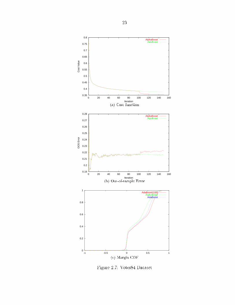
Table 2.2 shows the �nal values obtained by the two algorithms. As expected,AlphaBoost was able to achieve signi�cantly lower value of the cost function. ThoughAdaBoost achieved better out-of-sample error than AlphaBoost, the error bars aretoo high in these limited datasets to make any statistically signi�cant conclusions.Figures 2.3�2.8 show the cost function value and out-of-sample error as a functionof the number of iterations. For the �rst 100 iterations, AdaBoost and AlphaBoostperform exactly the same, so the curves coincide for this period. The cost functiontakes a steep dip around iteration 101 for AlphaBoost when it starts doing conjugate

16
1 2 3 4 5 6 7 8 9 100
0.02
0.04
0.06
0.08
0.1
0.12
Cos
t Val
ue
AdaBoostAlphaBoost
(a) Cost function value obtained by AdaBoost and Al-phaBoost
1 2 3 4 5 6 7 8 9 100
0.01
0.02
0.03
0.04
0.05
0.06
0.07
0.08
0.09
0.1
π
AdaBoostAlphaBoost
(b) Out-of-sample error obtained by AdBoost and Alpha-Boost
Figure 2.1: Performance of AlphaBoost and AdaBoost on a Target Generated byDEngin

17
0
0.1
0.2
0.3
0.4
0.5
0.6
0.7
0.8
0.9
1
0 20 40 60 80 100 120 140 160
Cos
t Val
ue
Iteration#
AlphaBoostAdaBoost
(a) Cost-function value at each iteration
0.15
0.2
0.25
0.3
0.35
0.4
0 20 40 60 80 100 120 140 160
Out
of S
ampl
e E
rror
Iteration#
AlphaBoostAdaBoost
(b) Out-of-sample error at each iteration
Figure 2.2: Performance of AlphaBoost and AdaBoost on a Typical Target

18
Table 2.2: Experimental Results on UCI Data SetsData Set Algorithm Cost π min(∆) ∆
Pima Indian AlphaBoost 0.5139 0.2638 −0.0979 0.0658AdaBoost 0.5763 0.2463 −0.1576 0.1023
Sonar AlphaBoost 0 0.1833 0.1099 0.2128
AdaBoost 0.0003 0.167 0.1088 0.2099Cleveland AlphaBoost 0.0386 0.2421 −0.183 0.0979
AdaBoost 0.0651 0.2047 −0.0747 0.1366
Ionosphere AlphaBoost 0 0.1 0.0652 0.1849AdaBoost 0.0094 0.0894 0.0459 0.1886
Vote AlphaBoost 0.3576 0.2222 −0.1359 0.2724AdaBoost 0.3756 0.2155 −0.1757 0.3104
Cancer AlphaBoost 0.0015 0.0483 −0.0052 0.2377AdaBoost 0.0509 0.0419 −0.0511 0.2638
gradient descent. The out-of-sample error increases during this stage. Also shown arethe distribution of the margins at the end of 100 iterations of AdaBoost, and at theend of 100 iterations of AdaBoost and 50 iterations of conjugate gradient descent. Thedistribution of the margins at the end of 100 iterations of AdaBoost is the startingpoint for both the algorithms, and from that point forward, they do di�erent thingsfor the next 50 iterations. AlphaBoost tends to maximize the minimum margin betterthan AdaBoost at the expense of lowering the maximum margin.
2.5.4 Discussion
The results of this section indicate that aggressively optimizing the cost function inboosting leads to worsening of the performance. The AlphaBoost ensemble uses theexact same weak hypothesis as the AdaBoost ensemble, so there is no additionalcomplexity that was introduced by the alpha-descent step. The only explanation forthis result is that the soft-min cost function tends to over�t. These results agreewith the �ndings of Li et al. [2003], where conjugate descent is used, but there thehypotheses used are di�erent from that of AdaBoost. This, however, does not refutethe margin theory explanation, as we are optimizing on one particular cost functionof the margin. The margin explanation relies on the reasoning that large margins are

19
0.5
0.55
0.6
0.65
0.7
0.75
0.8
0.85
0.9
0 20 40 60 80 100 120 140 160
Cos
t Val
ue
Iteration
AlphaBoostAdaBoost
(a) Cost function
0.24
0.245
0.25
0.255
0.26
0.265
0.27
0.275
0.28
0 20 40 60 80 100 120 140 160
OO
S E
rror
Iteration
AlphaBoostAdaBoost
(b) Out-of-sample Error
0
0.2
0.4
0.6
0.8
1
-1 -0.5 0 0.5 1
AdaBoost(100)AlphaBoost
AdaBoost
(c) Margin CDF
Figure 2.3: Pima Indian Diabetes DataSet

20
0
0.1
0.2
0.3
0.4
0.5
0.6
0 20 40 60 80 100 120 140 160
Cos
t Val
ue
Iteration
AlphaBoostAdaBoost
(a) Cost function
0.04
0.045
0.05
0.055
0.06
0.065
0.07
0.075
0.08
0.085
0 20 40 60 80 100 120 140 160
OO
S E
rror
Iteration
AlphaBoostAdaBoost
(b) Out-of-sample Error
0
0.2
0.4
0.6
0.8
1
-1 -0.5 0 0.5 1
AdaBoost(100)AlphaBoost
AdaBoost
(c) Margin CDF
Figure 2.4: Wisconsin Breast DataSet

21
0
0.1
0.2
0.3
0.4
0.5
0.6
0.7
0.8
0.9
0 20 40 60 80 100 120 140 160
Cos
t Val
ue
Iteration
AlphaBoostAdaBoost
(a) Cost function
0.16
0.18
0.2
0.22
0.24
0.26
0.28
0.3
0 20 40 60 80 100 120 140 160
OO
S E
rror
Iteration
AlphaBoostAdaBoost
(b) Out-of-sample Error
0
0.2
0.4
0.6
0.8
1
-1 -0.5 0 0.5 1
AdaBoost(100)AlphaBoost
AdaBoost
(c) Margin CDF
Figure 2.5: Sonar DataSet

22
0
0.1
0.2
0.3
0.4
0.5
0.6
0.7
0.8
0 20 40 60 80 100 120 140 160
Cos
t Val
ue
Iteration
AlphaBoostAdaBoost
(a) Cost function
0.08
0.09
0.1
0.11
0.12
0.13
0.14
0.15
0.16
0.17
0.18
0 20 40 60 80 100 120 140 160
OO
S E
rror
Iteration
AlphaBoostAdaBoost
(b) Out-of-sample Error
0
0.2
0.4
0.6
0.8
1
-1 -0.5 0 0.5 1
AdaBoost(100)AlphaBoost
AdaBoost
(c) Margin CDF
Figure 2.6: IonoSphere DataSet
23
0.35
0.4
0.45
0.5
0.55
0.6
0.65
0.7
0.75
0.8
0 20 40 60 80 100 120 140 160
Cos
t Val
ue
Iteration
AlphaBoostAdaBoost
(a) Cost function
0.19
0.2
0.21
0.22
0.23
0.24
0.25
0.26
0.27
0.28
0 20 40 60 80 100 120 140 160
OO
S E
rror
Iteration
AlphaBoostAdaBoost
(b) Out-of-sample Error
0
0.2
0.4
0.6
0.8
1
-1 -0.5 0 0.5 1
AdaBoost(100)AlphaBoost
AdaBoost
(c) Margin CDF
Figure 2.7: Votes84 Dataset

24
0
0.1
0.2
0.3
0.4
0.5
0.6
0.7
0.8
0.9
0 20 40 60 80 100 120 140 160
Cos
t Val
ue
Iteration
AlphaBoostAdaBoost
(a) Cost function
0.19
0.2
0.21
0.22
0.23
0.24
0.25
0.26
0.27
0 20 40 60 80 100 120 140 160
OO
S E
rror
Iteration
AlphaBoostAdaBoost
(b) Out-of-sample Error
0
0.2
0.4
0.6
0.8
1
-1 -0.5 0 0.5 1
AdaBoost(100)AlphaBoost
AdaBoost
(c) Margin CDF
Figure 2.8: Cleveland Heart Dataset

25
good for generalization. If we can show that optimizing any possible cost function ofthe margin would lead to bad generalization, this would refute the margin explanation.
2.6 DLPBoost
DLPBoost is an extension of AdaBoost which optimizes the margin distribution pro-duced by AdaBoost. It has been expressly designed to test the margin explanationfor the performance of AdaBoost. We have seen in the case of AlphaBoost thatdecreasing the cost function leads to larger minimum margin, but at the expense ofdecreasing the margin of some of the points. In most of the extensions and variants ofAdaBoost, the margin distribution produced does not dominate the margin distribu-tion of AdaBoost. We say that a distribution P1 dominates another distribution P2 ifP1(t) ≤ P2(t),∀t. As a result, there are some cost functions of the margin that wouldbe worsened by the variant. The only algorithm which could produce a better margindistribution was Arc-gv [Breiman 1998]. This algorithm was, however, criticized forproducing complex hypotheses and hence the increase in error was attributed to theadditional complexity used [Reyzin and Schapire 2006]. This is an important consid-eration in the design of DLPBoost. We want to make sure that the di�erence in thesolutions of AdaBoost and DLPBoost can only be accounted for by the di�erence inthe margins. It is therefore crucial to keep all other factors constant.
In DLPBoost, we provide an algorithm which consistently improves the entiredistribution of the margins. This condition ensures that DLPBoost has a bettermargin cost than AdaBoost for any possible de�nition of margin cost. Thus, all themargin bounds for AdaBoost would hold for DLPBoost, and as the complexity termsare not changed, the bounds become tighter. This would lead to better performanceif the margin explanation is true.
2.6.1 Algorithm
DLPBoost uses the AdaBoost solution as the starting point and optimizes the maxi-mum margin subject to constraints on the individual margins. The general problem of

26Algorithm 4 DLPBoostGiven (x1, y1), ..., (xN , yN)Run AdaBoost/AnyBoost for T iterations to get (h1, ..., hT ) and (α∗
1, ..., α∗T )
De�ne m(α, i) =∑T
t=1 yiαtht(xi)Solve the linear programming problem
maxα
∑Ni=1 m(α, i)
Subject to constraintsm(α, i) ≥ m(α∗, i)∑
αt = 1,αt ≥ 0
improving the margin distribution is very hard, optimization-wise, as it also involvesa combinatorial component. So, instead we set up a restricted problem in which werequire that the margin on none of the points is decreased. Any solution of the latterproblem would be a feasible solution for the original problem, though it might not beoptimal. Our goal here is to produce better margin distribution, and the restrictedsetup ensures that any solution we produce would have margin distributions at leastas good as those of the AdaBoost solution.
Algorithm 4 illustrates DLPBoost. The base classi�ers produced by DLPBoostare the exact same as the one produced by AdaBoost, and, by design, the margin ofeach training example is not reduced. Thus, by de�nition, DLPBoost does not �cheat�on the complexity and produces a solution which dominates (or at least equals) themargin distribution produced by AdaBoost.
2.6.2 Properties of DLPBoost
DLPBoost uses linear programming to �nd new weights for the hypotheses whichwould maximize the average margin, while ensuring that all the training exampleshave a margin at least as large as that of the AdaBoost solution. The weights gen-erated by AdaBoost, α∗, are a feasible solution to the optimization problem in DLP-Boost. The simplex procedure which is used to solve the optimization starts with azero solution, i.e., all the weights are initially zero. It then makes each of the weightsnon-zero, one at a time, until it �nds the optimal solution. One interesting byprod-uct of this procedure is that the �nal solution produced by DLPBoost would have a

27
smaller number of hypotheses with non-zero weights. This is a very useful feature,both theoretically and practically. Theoretically it means that the DLPBoost solutionhas a smaller dimensional complexity than the AdaBoost solution. In many practicalsituations, like visual recognition, where real-time processing of the data is critical,the DLPBoost solution can be useful as it tends to have a smaller ensemble size.
One of the interesting aspects of the DLPBoost setup is that the function beingoptimized is ad hoc. The important thing is to �nd a non-trivial feasible solution tothe constraints. The trivial solution in this case would be the AdaBoost solution inwhich all the inequalities are exactly satis�ed. We have used the average margin asthe goal, but we can use any general linear combination of the margins as the goaland still have a working setup. The most general setup would be a Multi-objectiveoptimization setup, in which we can maximize the margin on each point. There arepopular algorithms [Deb et al. 2002] to solve this kind of problem but we do not usethose, as the added advantage of a sparse solution generated by linear programming isvery appealing in our case. In addition, any non-trivial feasible solution would be anadded improvement on the margin distribution and serve the purpose of our analysis.
2.6.3 Relationship to Margin Theory
All the bounds discussed in section 2.4 hold for DLPBoost. For DLPBoost, by de�-nition
∀δPS[yFD(x) ≤ δ] ≤ PS[yFA(x) ≤ δ]
(where FD is the DLPBoost solution and FA is the AdaBoost solution). Hence wehave that the bound on the generalization error of DLPBoost is smaller than thebound on the generalization error of AdaBoost.
The setup of DLPBoost is a very optimistic one. It is a very constrained op-timization problem, as the number of constraints is of the the order of number ofexamples in the dataset. An improvement in all the margins would indicate that theoptimization procedure used in AdaBoost is very ine�cient. The design of DLPBoostensures that we do not introduce any additional complexity in the solution. Arc-GV,

28
which can also be used to generate ensembles with better margin distribution, hasbeen criticized for using additional hypothesis complexity [Reyzin and Schapire 2006].It also uses hypotheses which are di�erent from those used by AdaBoost, and so it isplausible that the solution generated is more complicated, thus any negative resultsthere might not contradict the margin explanation. In DLPBoost, we have isolatedthe margin explanation and any di�erence in performance can only be accounted forby the di�erence in the margin distributions. This would give us a fair evaluation ofthe margin explanation.
2.6.4 Experiments with Margins
We study the behavior of the margins and the solution produced by DLPBoost.Figures 2.9, 2.10 and 2.11 show the margins and the weights on the hypotheses ob-tained by AdaBoost and DLPBoost on the WDBC dataset. In this setup, we weightthe margins of the points in the linear programming setup by their cost function.This weighing promotes the points with smaller margin. The out-of-sample errorsfor AdaBoost was 2.74% and for DLPBoost was 3.75%. The margin distribution forDLPBoost is clearly much better than that of AdaBoost, and from the �nal weightsobtained, we can see that the hypotheses removed from the AdaBoost solution byDLPBoost had signi�cant weights assigned to them. Figure 2.10 shows the weightsassigned by the two algorithms to the weak hypotheses which are indexed by theiteration number. It can be seen that DLPBoost emphasizes some hypotheses whichwere generated late in AdaBoost training and it also killed some of the hypotheseswhich were generated early. AdaBoost is a greedy iterative algorithm. This kindof behavior is expected, as AdaBoost has no way of going back and correcting theweights of hypotheses already generated. Note that the one-norm of both the solu-tions is normalized to one, and so the DLPBoost solution having a smaller numberof hypotheses (64, compared to the 168 of AdaBoost) has overall larger weights andthis result is for a single run.
Figures 2.12, 2.13 and 2.14 show the same results for one run on the Australian

29
0 0.1 0.2 0.3 0.4 0.5 0.6 0.7 0.8 0.9 10
0.1
0.2
0.3
0.4
0.5
0.6
0.7
0.8
0.9
1
margin
wdbc−300
AdaBoost
DLPBoost−CF
Figure 2.9: Margins Distribution for WDBC Dataset with 300 Training Points
0 20 40 60 80 100 120 140 160 180 2000
0.01
0.02
0.03
0.04
0.05
0.06
iteration #
alph
a(i)
wdbc−300 alphas
AdaBoostDLPBoost−CF
Figure 2.10: α for WDBC Dataset with 300 Training Points

30
0 20 40 60 80 100 120 140 160 180 2000
0.01
0.02
0.03
0.04
0.05
0.06
i
alph
a(i)
wdbc−300 alphas sorted
AdaBoost
DLPBoost−CF
Figure 2.11: α Distribution for WDBC Dataset with 300 Training Points
dataset. Here the errors for both the algorithms were 18.8% while the number ofhypotheses was reduced from 423 to 201. In this case, there is very small improvementin the margin distribution and the out-of-sample error did not change. The hypotheseskilled by the DLPBoost step had signi�cant weights.
This points to an inverse relationship between the margins and the out-of-sampleperformance. In the next two sections, we will investigate this relationship in detailand give statistically signi�cant results.
2.6.5 Experiments with Arti�cial Datasets
We test the performance of DLPBoost and compare it with that of AdaBoost on afew arti�cial datasets.
2.6.5.1 Arti�cial Datasets Used
We used the following arti�cial learning problems for evaluation the performance ofthe cloning process.
Yin-Yang is a round plate centered at (0, 0) and is partitioned into two classes. The

31
0 0.05 0.1 0.15 0.2 0.25 0.3 0.35 0.40
0.1
0.2
0.3
0.4
0.5
0.6
0.7
0.8
0.9
1aus−500 margins
margin
Figure 2.12: Margins Distribution for Australian Dataset with 500 Training Points
0 50 100 150 200 250 300 350 400 450 5000
0.01
0.02
0.03
0.04
0.05
0.06
0.07aus−500 alphas
iteration #
alph
a(i)
Figure 2.13: α for Australian Dataset with 500 Training Points

32
0 50 100 150 200 250 300 350 400 450 5000
0.01
0.02
0.03
0.04
0.05
0.06
0.07aus−500 alphas
i
alph
a(i)
Figure 2.14: α Distribution for Australian Dataset with 500 Training Points
�rst class includes all points (x1, x2) which satis�es
(d+ ≤ r) ∨(
r < d− ≤ R2
)
∨(
x2 > 0 ∧ d+ > R2
)
,
where the radius of the plate is R = 1 and the radius of the two small circles isr = 0.18, d+ =
√
(x1 − R2)2 + x2
2 and d− =√
(x1 + R2)2 + x2
2.
LeftSin ([Merler et al. 2004]) partitions [−10, 10]× [−5, 5] into two class regions withthe boundary
x2 =
2 sin 3x1, if x1 < 0;
0, if x1 ≥ 0.
TwoNorm ([Breiman 1996]) is a 20-dimensional, 2-class classi�cation dataset. Eachclass is drawn from a multivariate normal distribution with unit variance. Class1 has mean (a, a, ..a) while Class 2 has mean (−a,−a, ..−a), where a = 2/
√20.
The arti�cial learning problems can be used to generate independent datasets fromthe same target to achieve statistically signi�cant results.

33
Figure 2.15: YinYang Dataset
Figure 2.16: LeftSin Dataset
34
0 200 400 600 800 1000 1200 1400 1600 1800 2000 2200−2
0
2
4
6
8
10
12
14x 10
−3
N
π dlp−
π ada
(a) Change in π
0 200 400 600 800 1000 1200 1400 1600 1800 2000 22000
0.005
0.01
0.015
0.02
0.025
0.03
0.035
0.04
0.045
N
(b) Change in Average Margin
0 200 400 600 800 1000 1200 1400 1600 1800 2000 22000
0.05
0.1
0.15
0.2
0.25
N
(c) Maximum Change in Margin
200 400 600 800 1000 1200 1400 1600 1800 2000 22000
50
100
150
200
250
300
350
400
450
N
AdaBoostDLPBoost
(d) Size of Ensemble
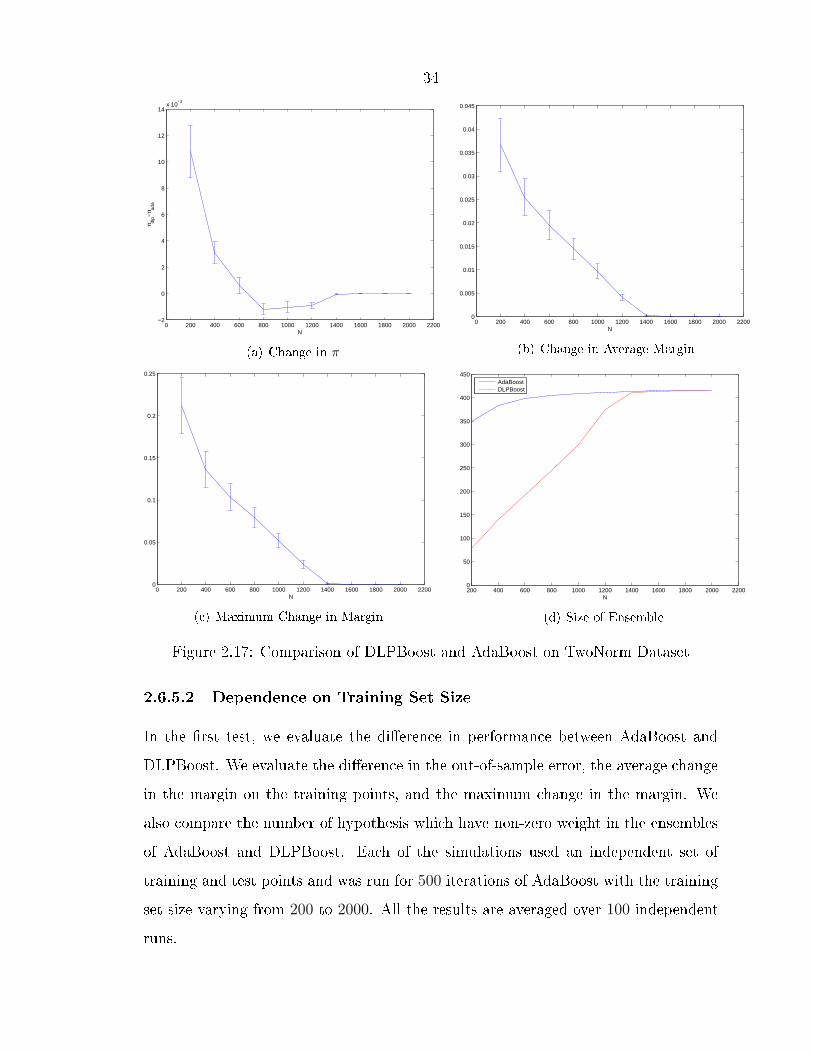
Figure 2.17: Comparison of DLPBoost and AdaBoost on TwoNorm Dataset
2.6.5.2 Dependence on Training Set Size
In the �rst test, we evaluate the di�erence in performance between AdaBoost andDLPBoost. We evaluate the di�erence in the out-of-sample error, the average changein the margin on the training points, and the maximum change in the margin. Wealso compare the number of hypothesis which have non-zero weight in the ensemblesof AdaBoost and DLPBoost. Each of the simulations used an independent set oftraining and test points and was run for 500 iterations of AdaBoost with the trainingset size varying from 200 to 2000. All the results are averaged over 100 independentruns.

35
0 500 1000 1500 2000 2500 3000−1
0
1
2
3
4
5x 10
−5
N
π dlp−
π ada
(a) Change in π
0 500 1000 1500 2000 2500 30000
0.2
0.4
0.6
0.8
1
1.2x 10
−3
N
(b) Change in Average Margin
0 500 1000 1500 2000 2500 30000
0.5
1
1.5
2
2.5
3
3.5
4
4.5
5x 10
−3
N
(c) Maximum Change in Margin
0 500 1000 1500 2000 2500 30000
1
2
3
4
5
6
7
8
9
10
N
AdaBoostDLPBoost
(d) Size of Ensemble
Figure 2.18: Comparison of DLPBoost and AdaBoost on YinYang Dataset
Figure 2.17 shows the results for the TwoNorm dataset, which is 20-dimensional.We observe that the out-of-sample performance of DLPBoost is consistently worsethan that of AdaBoost. The di�erence goes down to zero as the training set sizeincreases. The increase in the average margins and the maximum change in themargin are indications of the ine�ciency of AdaBoost in optimizing the margins. Wecan also see the number of hypotheses used by the DLPBoost increase as we increasethe training set size.
We observe similar behavior on the Yin-Yang dataset (Figure 2.18) which is 2-dimensional, except in this case the change in the out-of-sample error is very small and

36
0 200 400 600 800 1000 1200 1400 1600 1800 2000 22000
0.002
0.004
0.006
0.008
0.01
0.012
0.014
N
π dlp−
π ada
(a) Change in π
0 200 400 600 800 1000 1200 1400 1600 1800 2000 22000
0.01
0.02
0.03
0.04
0.05
0.06
N
(b) Change in Average Margin
0 200 400 600 800 1000 1200 1400 1600 1800 2000 22000
0.05
0.1
0.15
0.2
0.25
N
(c) Maximum Change in Margin
200 400 600 800 1000 1200 1400 1600 1800 2000 22000
50
100
150
200
250
300
350
400
450
N
AdaBoostDLPBoost
(d) Size of Ensemble
Figure 2.19: Comparison of DLPBoost and AdaBoost on RingNorm Dataset
not signi�cantly di�erent from 0 in most of the cases. Another observation here is thateven for 3000 points in the training set, the DLPBoost solution does not use all the 500
hypotheses. In the TwoNorm case, with large training sets, the DLPBoost solutionused all the 500 hypotheses in its solution. Hence the ine�ciency in AdaBoost is afunction of the complexity of the dataset and the number of examples in the trainingpoints. AdaBoost ended up using 500 hypotheses to explain the Yin-Yang dataset of1000 examples or more which is a clear indication of over �tting. DLPBoost, on theother hand, adjusts its complexity based on the complexity of the dataset.
The RingNorm dataset is more complicated than the TwoNorm dataset and it is

37
0 200 400 600 800 1000 1200 1400 1600 1800 2000 22000
0.001
0.002
0.003
0.004
0.005
0.006
0.007
0.008
0.009
0.01
T
π dlp−
π ada
(a) Change in π
0 200 400 600 800 1000 1200 1400 1600 1800 2000 22000
0.01
0.02
0.03
0.04
0.05
0.06
T
(b) Change in Average Margin
0 200 400 600 800 1000 1200 1400 1600 1800 2000 22000
0.05
0.1
0.15
0.2
0.25
T
(c) Maximum Change in Margin
200 400 600 800 1000 1200 1400 1600 1800 2000 22000
500
1000
1500
T
AdaBoostDLPBoost
(d) Size of Ensemble
Figure 2.20: Comparison of DLPBoost and AdaBoost on TwoNorm Dataset
re�ected in the results in Figure 2.19.
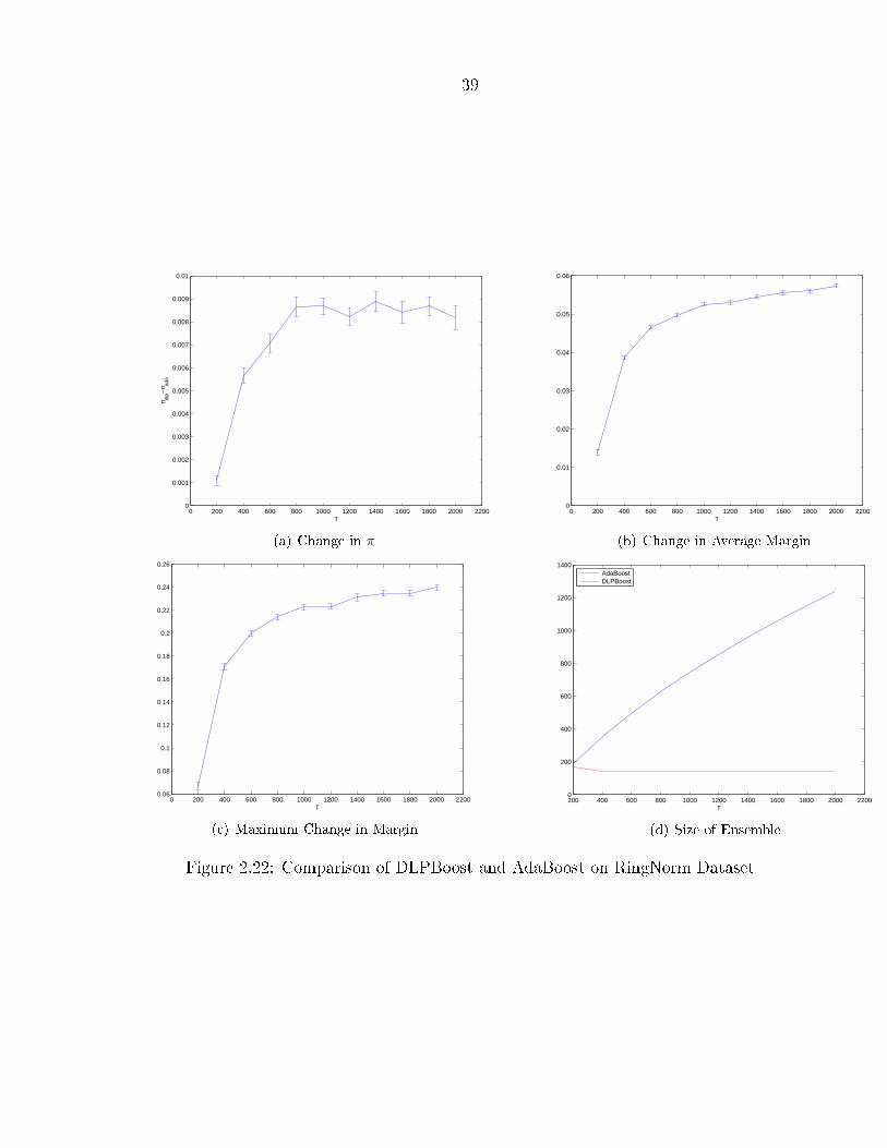
2.6.5.3 Dependence on the Ensemble Size
We ran the same experiments by �xing the ensemble size to 500 and varying thenumber of iterations given to AdaBoost. Figures (2.20�2.22) give the results of theseexperiments.
Here we observe that as we use more and more hypotheses in the AdaBoost en-semble, DLPBoost is able to get more improvement in the margins. This also leadsto a consistent worsening of performance in the TwoNorm case. It is interesting to

38
0 200 400 600 800 1000 1200 1400 1600 1800 2000 2200−2
0
2
4
6
8
10
12
14
16x 10
−4
T
π dlp−
π ada
(a) Change in π
0 200 400 600 800 1000 1200 1400 1600 1800 2000 22000
0.002
0.004
0.006
0.008
0.01
0.012
0.014
T
(b) Change in Average Margin
0 200 400 600 800 1000 1200 1400 1600 1800 2000 22000.03
0.04
0.05
0.06
0.07
0.08
0.09
0.1
T
(c) Maximum Change in Margin
200 400 600 800 1000 1200 1400 1600 1800 2000 22000
200
400
600
800
1000
1200
1400
1600
1800
T
AdaBoostDLPBoost
(d) Size of Ensemble
Figure 2.21: Comparison of DLPBoost and AdaBoost on YinYang Dataset
39
0 200 400 600 800 1000 1200 1400 1600 1800 2000 22000
0.001
0.002
0.003
0.004
0.005
0.006
0.007
0.008
0.009
0.01
T
π dlp−
π ada
(a) Change in π
0 200 400 600 800 1000 1200 1400 1600 1800 2000 22000
0.01
0.02
0.03
0.04
0.05
0.06
T
(b) Change in Average Margin
0 200 400 600 800 1000 1200 1400 1600 1800 2000 22000.06
0.08
0.1
0.12
0.14
0.16
0.18
0.2
0.22
0.24
0.26
T
(c) Maximum Change in Margin
200 400 600 800 1000 1200 1400 1600 1800 2000 22000
200
400
600
800
1000
1200
1400
T
AdaBoostDLPBoost
(d) Size of Ensemble
Figure 2.22: Comparison of DLPBoost and AdaBoost on RingNorm Dataset

40
Table 2.3: Experimental Results on UCI Data SetsData Set Algorithm Size of Ensemble π ∆ Maximum Change
Pima Indian DLPBoost 99.12(0.06) 0.2466(0.003) 0.00829 0.0061AdaBoost 99.54(0.06) 0.2462(0.003) 0.0829 -
Sonar DLPBoost 78.78(0.05) 0.1643(0.0004) 0.2221 0.1374AdaBoost 125.93(0.06) 0.1562(0.0005) 0.1978 -
Cleveland DLPBoost 68.33(0.04) 0.1963(0.0005) 0.1210 0.0038AdaBoost 68.75(0.04) 0.1962(0.0005) 0.1201 -
Ionosphere DLPBoost 95.47(0.07) 0.0941(0.0003) 0.1801 0.0259AdaBoost 107.76(0.05) 0.0904(0.0003) 0.1749 -
Vote DLPBoost 15.31(0.04) 0.0621(0.002) 0.4457 0.0166AdaBoost 15.85(0.05) 0.0619(0.0002) 0.4422 -
Cancer DLPBoost 75.37(0.08) 0.028(0.0001) 0.3797 0.1087AdaBoost 102.69(0.06) 0.026(0.0002) 0.3454 -
note that the DLPBoost solution uses almost the same number of hypothesis irre-spective of the number of hypothesis in the AdaBoost ensemble. This also shows thatthe number of hypotheses required to explain the dataset is dependent only on thenumber of training points and the complexity of the dataset.
2.6.6 Experiments on Real World Datasets
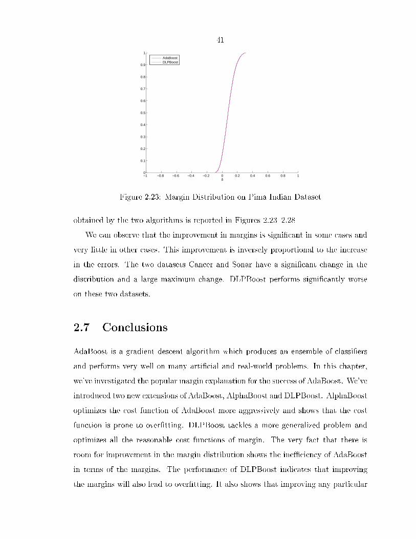
We tested DLPBoost on the same six datasets from the UCI machine learning repos-itory [Blake and Merz 1998] used in Section 2.5.3. Decision stumps were used as thebase learner in all the experiments. For the experiments, the dataset was randomlydivided into two sets of size 80% and 20%, used for training and testing the algo-rithms. All the results are averaged over 100 di�erent splits to obtain the error bars.The AdaBoost algorithm was run for 250 iterations and the size of the ensemble isde�ned as the number of unique hypothesis in the ensemble. Table 2.3 summarizesthe results. The maximum change column refers to the maximum increase in themargin of any point in the training set. The values in the parentheses denotes thesize of the standard error bar.
The average and the maximum change are just two statistics of the margin distri-bution which are most informative to the discussion. The entire margin distribution
41
−1 −0.8 −0.6 −0.4 −0.2 0 0.2 0.4 0.6 0.8 10
0.1
0.2
0.3
0.4
0.5
0.6
0.7
0.8
0.9
1
δ
AdaBoostDLPBoost
Figure 2.23: Margin Distribution on Pima Indian Dataset
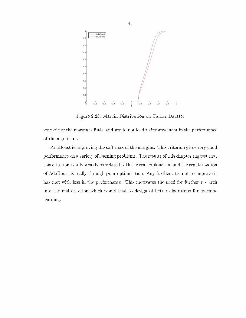
obtained by the two algorithms is reported in Figures 2.23�2.28We can observe that the improvement in margins is signi�cant in some cases and
very little in other cases. This improvement is inversely proportional to the increasein the errors. The two datasets Cancer and Sonar have a signi�cant change in thedistribution and a large maximum change. DLPBoost performs signi�cantly worseon these two datasets.
2.7 Conclusions
AdaBoost is a gradient descent algorithm which produces an ensemble of classi�ersand performs very well on many arti�cial and real-world problems. In this chapter,we've investigated the popular margin explanation for the success of AdaBoost. We'veintroduced two new extensions of AdaBoost, AlphaBoost and DLPBoost. AlphaBoostoptimizes the cost function of AdaBoost more aggressively and shows that the costfunction is prone to over�tting. DLPBoost tackles a more generalized problem andoptimizes all the reasonable cost functions of margin. The very fact that there isroom for improvement in the margin distribution shows the ine�ciency of AdaBoostin terms of the margins. The performance of DLPBoost indicates that improvingthe margins will also lead to over�tting. It also shows that improving any particular

42
−1 −0.8 −0.6 −0.4 −0.2 0 0.2 0.4 0.6 0.8 10
0.1
0.2
0.3
0.4
0.5
0.6
0.7
0.8
0.9
1
δ
AdaBoostDLPBoost
Figure 2.24: Margin Distribution on Sonar Dataset
−1 −0.8 −0.6 −0.4 −0.2 0 0.2 0.4 0.6 0.8 10
0.1
0.2
0.3
0.4
0.5
0.6
0.7
0.8
0.9
1
δ
AdaBoostDLPBoost
Figure 2.25: Margin Distribution on Cleveland Dataset

43
−1 −0.8 −0.6 −0.4 −0.2 0 0.2 0.4 0.6 0.8 10
0.1
0.2
0.3
0.4
0.5
0.6
0.7
0.8
0.9
1
δ
AdaBoostDLPBoost
Figure 2.26: Margin Distribution on Ionosphere Dataset
−1 −0.8 −0.6 −0.4 −0.2 0 0.2 0.4 0.6 0.8 10
0.1
0.2
0.3
0.4
0.5
0.6
0.7
0.8
0.9
1
δ
AdaBoostDLPBoost
Figure 2.27: Margin Distribution on Voting Dataset
44
−1 −0.8 −0.6 −0.4 −0.2 0 0.2 0.4 0.6 0.8 10
0.1
0.2
0.3
0.4
0.5
0.6
0.7
0.8
0.9
1
δ
AdaBoostDLPBoost
Figure 2.28: Margin Distribution on Cancer Dataset
statistic of the margin is futile and would not lead to improvement in the performanceof the algorithm.
AdaBoost is improving the soft-max of the margins. This criterion gives very goodperformance on a variety of learning problems. The results of this chapter suggest thatthis criterion is only weakly correlated with the real explanation and the regularizationof AdaBoost is really through poor optimization. Any further attempt to improve ithas met with loss in the performance. This motivates the need for further researchinto the real criterion which would lead to design of better algorithms for machinelearning.

45
Chapter 3
Adaptive Estimation UnderMonotonicity Constraints
3.1 Introduction
The typical learning problem takes examples of the target function as input informa-tion and produces a hypothesis that approximates the target as an output. In thischapter, we consider a generalization of this paradigm by taking di�erent types ofinformation as input, and producing only speci�c properties of the target as output.
Generalizing the typical learning paradigm in this way has theoretical and practi-cal merits. It is common in real-life situations that we would have access to heteroge-neous pieces of information, not only input-output data. For instance, monotonicityand symmetry properties are often encountered in modeling patterns of capital mar-kets and credit ratings [Abu-Mostafa 1995; 2001]. Input-output examples comingfrom historical data are but one of the pieces of information available in such appli-cations. It is also commonplace that we are not interested in learning the entirety ofthe target function, and would be better o� focusing on only some speci�c propertiesof the target function of particular interest and achieving better performance in thismanner. For instance, instead of trying to estimate an entire utility curve, we maybe only interested in the threshold values at which the curve goes above or below acritical value.
Another common feature encountered in the applications that we have considered
46
is that the data is very expensive or time consuming to obtain. In many such cases,adaptive sampling is employed to get better performance with very small sample size[Cohn et al. 1994, MacKay 1992]. In this chapter, we will describe a new adaptivelearning algorithm for estimating a threshold -like parameter from a monotonic func-tion. The algorithm works by adaptively minimizing the uncertainty in the estimatevia its entropy. This, combined with a provably consistent learning algorithm, is ableto achieve signi�cant improvement in performance over the existing methods.
3.1.1 Applications
This problem is very general in nature and appears in many di�erent forms in Psy-chophysics [Palmer 1999, Klein 2001] , Standardized testing like the GRE [Baker2001], adaptive pricing, and drug testing [Cox 1987]. In all these applications, there'sa stimulus, and at each stimulus there is a probability of obtaining a positive response.This probability is known to be monotonically increasing.
The most popular application of these methods is in the �eld of drug testing. It isknown that the probability of a treatment curing a disease is monotonic in the levelof dosage in the treatment, within a certain range. It is desirable to obtain a correctdose level which will induce a certain probability of producing a cure. The samplesin this problem are very expensive and adaptive testing is generally the preferredapproach.
Standardized tests, like the SAT and the GRE, use adaptive testing to evaluatethe intelligence level of students. Item Response Theory [Lord 1980] models eachquestion that is presented in the test as an item and for each item, the probability ofa student correctly answering the question is monotonic in his intelligence. Each Itemhas a di�erent di�culty level, and the next item presented to the student is adaptivelychosen based on his or her performance on the previous items. A student's GRE orSAT score is de�ned as a di�culty level at which a student has a certain probabilityof correctly answering the questions.
Another �eld where this kind of problem occurs is in determining the optimal

47
discount level when pricing a product for sale. The probability of a customer buyinga certain product increases monotonically with the amount of discount o�ered. Inthis application, it is not necessary to go after the entire price elasticity curve todetermine the discount value at which the expected pro�t is su�cient to achieve asales goal.
All these applications have the common theme that the target is a monotonicfunction from which we can adaptively get Bernoulli samples which are otherwiseexpensive to obtain. In each of the cases, we are not interested in the whole targetbut only in a critical value of the input.
3.1.2 Monotonic Estimation Setup
Consider a family of Bernoulli random variables V (x) with parameters p(x) whichare known to be monotonic in x, i.e., p(x) ≤ p(y) for x < y. Suppose for X =
{x1, .., xM}, we have m(xi) independent samples of V (xi). We can estimate p(xi)
as the average number of positive responses yi. If the number of samples is smallthen these averages will not necessarily satisfy the monotonicity condition. We willdiscuss the existing methods which take advantage of the monotonicity restriction onthe estimation process and introduce a new regularized algorithm.
3.1.3 Threshold Function
We have a target function p : X → Y which is monotonically increasing. A thresholdfunctional θ maps a function p to X. The threshold function can take many forms,the most common among them are:
Critical Value Crossing Functional. This is the most common form of the thresh-old. The problem here is to estimate the input value at which the monotonicfunction goes above a certain value. For example θ(h) = h−1(0.612) measuresthe point at which the function crosses 0.612.
Trade-O� Functional. This takes the form θ(h) = argmaxxG(x)p(x), where G(x)

48
is a �xed known function and is usually monotonically non increasing. Thiskind of functional appears in the adaptive pricing problem, where the goal is tomaximize expected pro�t. If the probability of a sale upon o�ering a discountrate of x is p(x), then the expected pro�t is given by θ(x) = (1 − x)p(x).
3.1.4 Adaptive Learning Setup
In the adaptive learning setup, given an input point x ∈ X, we can obtain a noisyoutput y = p(x) + ε(x), where ε is a zero mean input dependent noise function.For the scope of this chapter, Y = {0, 1} and the noisy sample at x would be aBernoulli random variable with mean p(x), i.e., y|x = B(p(x)). This scenario iscommon in various real-world situations in which we can only measure the outcomeof the experiment (success or failure) and wish to estimate the underlying probabilityof success. For adaptive sampling, we are allowed to choose the location of the nextsample based on the previous data samples and any prior knowledge that we mighthave. In the following sections, we will introduce existing and new methods to sampleadaptively for monotonic estimation.
3.2 Existing Algorithms for Estimation under Mono-tonicity Constraint
Most of the currently used methods employ a parametric estimation [Finney 1971,Wichmann and Hill 2001] technique for �tting a monotonic function to the data. Themain advantage of this method is the ease in estimation and the high regularizationability for small sample sizes, as there are only a small number of parameters to �t.
An alternate approach is to use the non-parametric method, MonFit (also knownin literature as isotonic regression [Barlow et al. 1972]) in which we do not assumeanything about the target function. This method has better performance as it doesnot have the additional bias from the parametric assumption and is able to regularizethe estimate by enforcing the monotonicity constraint. This method is not used much

49
in practice, as the output from it is a step-wise linear function with a lot of �at regions,which is not very intuitive, although optimal in the absence of any assumptions aboutthe setup.
3.2.1 Parametric Estimation
Parametric estimation is the most popular method used in practice. The methodassumes a parametric form for the target and estimates the parameters using thedata. This gives the entire target as the output. In most of the parametric methods,the target function is assumed to be coming from a 2-parameter family of functions.The parameters are estimated from the data and the threshold or the threshold-likequantity can be computed from the inverse of the parametric function. The mostcommonly used methods for estimating the parameters are probit analysis [Finney1971] and maximum likelihood [Watson 1971, Wichmann and Hill 2001]. In thisthesis, we will use the maximum likelihood method with the two parameter logisticfamily [Hastie et al. 2001] as the model.
Flog = {f(x, a, b) = 1/(1 + e(x−a)/b)}
3.2.2 Non-Parametric Estimation
In the non-parametric approach (MonFit), [Barlow et al. 1972, Brunk 1955] the solu-tion is obtained by a maximum likelihood estimation under the constraints that theunderlying variables are monotonic. It is equivalent to �nding the closest monotonicseries in the mean square sense.
MonFit is an algorithm which solves the optimization problem
minµ
M∑
i=1
m(xi) [µi − yi]2 (3.1)

50
under the constraints
µi ≤ µj ∀i ≤ j
The MonFit estimator always exists and is unique. It has a closed-form solution[Barlow et al. 1972]
µ∗i = max
s≤imint≥i
Av(s, t) (3.2)
whereAv(s, t) =
∑
i m(xi)yi∑
i m(xi)
The solution can be computed in linear time by the Pool Adjusted Vector Algo-rithm [Barlow et al. 1972]. The algorithm starts out with a pool of points, one foreach of the design points xi. The value of the estimator for each pool is computedas the average value of the points inside the pool. If there are two consecutive poolswhich violate the monotonicity restriction, then these pools are merged into one. Thisprocedure is repeated until all consecutive pools obey the monotonicity restriction.
Theorem 1 Given examples from a family of Bernoulli random variables with mono-tonic probability, the MonFit estimate has a lower or equal mean square error thanthe naive estimate
Proof Let us consider the case when we have one example in each bin. We willdenote the target as pi = p(xi) and assume that each bin has one sample, i.e., m(xi) =
1. Suppose the �rst pool of the MonFit estimate contains k points, then the partialmean square error made in the �rst pool for the MonFit case would be
e1mbt =
k∑
i=1
(y − pi)2
where y =∑k
i=1 yi is the average pooled value which is assigned to each bin in the�rst pool.
The partial mean square error by the naive estimate would be

51
e1naive =
k∑
i=1
(yi − pi)2
The di�erence between the errors can be written as
e1naive − e1
mbt =1
k
k∑
i,j=1
(yi − yj)2 +
2
k
k∑
i=1
k∑
j=i+1
(pi − pj)(yj − yi) (3.3)
Now, since the �rst k points were pooled, we have that
y1 ≥y1 + y2
2≥ y1 + y2 + y3
3≥ . . . ≥
∑ki=1 yi
k
From which we can conclude, that
y1 ≥ y2 ≥ y3 ≥ . . . ≥ yk
p′is are monotonic, therefore,
p1 ≤ p2 ≤ p3 ≤ . . . ≤ pk
So, each term in equation (3.3) is non-negative. So, we have that e1naive ≥ e1
mbt.The mean square error would be the sum of the partial mean square errors in each
pool, so enaive ≥ embt
For the general case, when each bin has a weight wi = m(xi), we can do similarcalculation and get
e1naive − e1
mbt =1
k
k∑
i,j=1
wiwj(yi − yj)2 +
2
k
k∑
i=1
k∑
j=i+1
wiwj(pi − pj)(yj − yi)
where, in this case,
e1mbt =
k∑
i=1
wi(y − pi)2

52
wherey =
∑ki=1 wiyi
∑ki=1 wi
and
e1naive =
k∑
i=1
wi(yi − pi)2
and the ordering on y′is still holds, so each term is again positive.
¤
Theorem 1 proves the advantage in enforcing the monotonicity constraint. Thenaive estimate is unbiased, and by enforcing the additional constraints the MonFitestimator becomes biased. However, the variance of the MonFit estimator is reduced.This result proves that overall, the increase in the bias is less than the correspondingdecrease in the variance, making MonFit a better option for minimizing the meansquare error.
The MonFit solution only gives the target values at the design points. To esti-mate the threshold, the function can be interpolated in any possible way. The mostcommon approach is to interpolate it linearly in between the design points, althoughmore sophisticated approaches are possible (like monotonic splines [Ramsay 1998]).We use linear interpolation because of its simplicity and the fact that we do not haveany a priori knowledge to choose one over another. Theorem 2 proves the consis-tency property of the MonFit estimate with constant interpolation but it can also beextended to linear interpolation.
Theorem 2 Let f(x) be a continuous non-decreasing function on (a, b). Let {xn}bea sequence of points dense in (a, b)with one observation made at each point. Let thevariance of the observed random variables be bounded. Let fn(x)be the estimate basedon the �rst n observations, de�ned to be constant between observation points andcontinuous from the left. If c > a and d < b, then
P
[
limn→∞
maxc≤t≤d
∣
∣
∣f(t) − f(t)
∣
∣
∣= 0
]
= 1
Proof See Brunk [1958]

53
3.3 Hybrid Estimation Procedure
The existing methods which we have discussed have their own advantages and disad-vantages. We introduce a hybrid estimation technique, which is a combination of theparametric and the nonparametric approaches that tries to combine the advantagesof both into one approach. We developed a regularized version of MonFit, which wecall Bounded Jump Regression, that uses jump parameters to smoothen and regu-larize the MonFit solution. Bounded jump regression with a heuristic for parameterselection is used here for estimation in the hybrid estimation procedure.
3.3.1 Bounded Jump Regression
One of the main drawbacks of the non-parametric approach is that the solution itproduces is a step function, which for many applications is non-smooth and tends tohave a lot of �at regions. Practically, this kind of behavior is unacceptable [Wichmannand Hill 2001]. In this section, we introduce a new approach to estimating the solutionwhich introduces a parameter to the MonFit algorithm in order to make it smooth.
The non-parametric estimation technique solves a least squares regression problemunder the monotonicity constraint. The monotonicity constraint ensures that thedi�erence between two consecutive estimates is positive. In this section we introduce ageneralization of this problem where the di�erence between two consecutive estimatesis bounded above and below by certain parameters.
3.3.1.1 De�nition
We de�ne the Bounded Jump Regression problem as follows
minµ
N∑
i=1
(µi − yi)2 (3.4)
Subject to the constraints that
δi ≤ µi+1 − µi ≤ ∆i ∀i = 0..N (3.5)

54
where µ0 and µN+1 are �xed constants and {δi, ∆i}Ni=1are parameters for the model.
3.3.1.2 Examples
Many of the regression problems can be expressed as a special case of the boundedjump regression problem. For regression of binomial probabilities which we are dealingwith in this chapter, we �x the boundary points µ0 = 0 and µN+1 = 1.
• When δi = −∞ and ∆i = ∞, the constraints are vacuous and the problemreduces to normal mean squares regression.
• When δi = 0 and ∆i = ∞, the constraints enforce the monotonicity on µ′is ,
and so, the problem reduces to monotonic regression.
• When δi = 1/N + 1, there is only one feasible solution and so there is noregression problem to solve.
3.3.1.3 Solving the BJR Problem
The BJR problem can be reduced to a quadratic optimization problem under boxconstraints by using suitable variable transformations. If we substitute
zi =pi+1 − pi − δi
1 − ∑Nt=0 δt
and
Ci =∆i − δi
1 − ∑
δt
and
Qij = min(N + 1 − i, N + 1 − j)
and
ynewi =
i∑
t=1
(
yt
1 − ∑Nr=0 δr
− δt
)

55
then, BJR can be reduced to
min1
2zT Qz − zT ynew
under the constraints that
0 ≤ z ≤ C
and
zT1 = 1
3.3.1.4 Special Cases
For the case when we have ∆i = ∞, the BJR can be reduced to monotonic regressionproblem and hence can be solved in linear time.
By using the transform
zi =pi −
∑it=1 δt
1 − ∑Nt=0 δt
and
ynewi =
yi −∑i
t=1 δt
1 − ∑Nr=0 δr
The BJR reduces to
minµ
N∑
i=1
(zi − ynewi )2 (3.6)
Subject to the constraints that
zi+1 − zi ≥ 0 ∀i = 0..N (3.7)

56
δ = 0
δ = 1/N
δ = −1
Figure 3.1: δ as a Complexity Parameter Controlling the Search Space
3.3.1.5 δ as a Complexity Parameter
Consider the case, when we have ∆i = ∞ , i.e., we're only bounding the minimumjump between two consecutive bins, and δi = δ for all i. For the case when we haveδ = −∞, BJR reduces to normal regression and the set of feasible solution is theentire R
N plane (or if we are working with probabilities, it will be [0, 1]N). As weincrease δ, the feasible region keeps shrinking. At δ = 0, the feasible region is theset of all monotonic functions, and when δi = 1/N + 1, the feasible region containsjust one solution. So, δ can be seen as a measure of complexity of the solution spaceand increasing delta will reduce the variance while increasing the bias. The numberof independent parameters in the feasible region can also be considered as a functionof δ. For δ = −∞, the number of independent parameters is N , and for δ = 1/N +1,it is zero. This gives us a continuous control over the bias and variance trade-o�.δ = −∞ corresponds to the zero bias solution and δ = 1/N + 1 corresponds to thezero variance solution.
57
3.3.2 Hybrid Estimation Algorithm
In the hybrid estimation algorithm we use bounded jump regression with the lowerbound δ as a parameter. By controlling δ, we are e�ectively controlling the size of thefeasible region and thus giving better generalization performance, especially whenwe have a small number of examples. The jump parameter denotes the minimumvalue of the gradient of the target function. As we have seen in 3.3.1.5 , it controlsthe search space in which the non-parametric algorithm searches for the optimalsolution. However, we have the same number of parameters as the number of bins Ifwe estimate all of them from the data, it would really be a non-parametric procedureas the number of parameters vary according to the data. To limit this, we use only asingle parameter and scale it di�erently for each bin. Estimating δ requires knowledgeabout the nature of the target function and we estimate δ using the parametric �t.
The δ parameter is the lower bound on the jump between bins, i.e. pi+1 − pi ≥ δi.This can be estimated by the gradient of the target function. We have
pi+1 − pi ≥ (xi+1 − xi) min(p′(x))
We estimate the gradient of the target function as the minimum of the gradientof the parametric solution. We set
δi ∝ (xi+1 − xi) minj
p(xj+1) − p(xj)
xj+1 − xj
The MonFit estimation algorithm does not take into account the change in inputvalue between the bins. The parametric method exploits the dependence nicely andreturns a function which depends on the location of the bins. This heuristic allowsus to introduce this dependence into the estimation procedure.
Ideally, if we have small number of samples then we should choose a smaller spaceto search in; as we get more and more examples, we can a�ord to expand the searchspace. We therefore decrease the jump parameter as we get more samples. In thelimit as we increase the number of samples, the hybrid estimation converges to the

58
Algorithm 5 HybridFit(x, y, m)• Input: x = (x1, .., xN), y = (y1, ..., yN), and m = (m1, ..., mN), where yi is theaverage number of positive responses out of mi samples which were taken at xi
� Let fl(x) be the best logistic �t for the data (x, y, m)
� Calculate d = minf(xj+1)−f(xj)
xj+1−xj, the minimum gradient estimate
� Let δi = dxi+1−xi
mi
� De�ne ynewi
=yi−
Pij=1
δj
1−PN
j=1δj
� Let z = MonFit(y, m)
� Return µhybridi = zi(1 − ∑N
j=1 δj) +∑i
j=1 δj
same solution as the monotonic regression. This allows us to derive the asymptoticproperties for the hybrid estimation, like consistency and convergence. We scale thegradient at any point by the inverse of the number of samples at that point.
3.3.3 Pseudo-Code and Properties
Algorithm 5 describes the hybrid estimation algorithm. The hybrid estimation algo-rithm inherits the asymptotic statistical properties from the MonFit estimator. Asthe number of samples increase densely in the region of interest, the δ parameter goesdown to zero.
Corollary 1 Let f(x) be a continuous non-decreasing function on (a, b). Let {xn}bea sequence of points dense in (a, b)with one observation made at each point. Let thevariance of the observed random variables be bounded. Let fn(x)be the hybrid estimatebased on the �rst n observations, de�ned to be constant between observation pointsand continuous from the left. If c > a and d < b, then
P
[
limn→∞
maxc≤t≤d
∣
∣
∣f(t) − f(t)
∣
∣
∣= 0
]
= 1

59
Proof Since, f is a continuous non-decreasing function on (a, b), the minimum ofthe gradient of the parametric estimate used in the estimation of δ would be bounded.The scaling factor is proportional to the di�erence between the consecutive samplepoints. Since the points are dense in the region, the minimum jump parameter wouldconverge to 0 as n → ∞. With these observations, the Corollary follows directly fromTheorem 2. ¤
3.3.4 Experimental Evaluation
We compared the hybrid estimation algorithm with the MonFit and the parametric�t algorithms. We compare the performance for various shapes of the target functionas shown in Table 3.1.
Table 3.1: Various Shapes of Target Function Used in the ComparisonLinear f(x) = x
Weibull f(x) = (1 − e−x2
)
NormCDF f(x) = Φ(x−0.50.25
)
Student-t Student's t distribution with 10 dofQuadratic f(x) = x2
TR f(x) =
2x2 x ≤ 0.5
1 − 2(1 − x)2 x > 0.5
Exponential f(x) = 1
1+ea−x
b
,a = 0.5, b = 0.05
Exponential2 f(x) = 1
1+ea−x
b
,a = 0.4, b = 0.1
For each of the targets, we compute the deviation in the estimates which is de�nedas
d(y, m) =N
∑
i=1
m(xi)(yi − pi)2/
N∑
i=1
m(xi)
Figure 3.2 shows the deviation when we have one sample per bin (i.e. m(xi) = 1)and Figure 3.3 shows the result when more samples are taken in the center than in

60
Linear Weibull NormCDF Student−t Quadratic TR Exp Exp20
0.01
0.02
0.03
0.04
0.05
0.06
Datasets
Dev
iatio
n
ParamFitMonFitHybridFit
Figure 3.2: Comparison of Various Monotonic Estimation Methods with 1 SamplePer Bin

61
Linear Weibull NormCDF Student−t Quadratic TR Exp Exp20
0.5
1
1.5
2
2.5
3
3.5x 10
−3
ParamFitMonFitHybridFit
Figure 3.3: Comparison of Various Monotonic Estimation Methods with m(xi) =min(i, N − i)

62
the corners (i.e. m(xi) = min(i, N − i)).We can see that hybrid �t generally outperforms both parametric and MonFit on
all the targets, as it uses information from both the parametric and MonFit to com-pute its estimate. The performance ParamFit depends on how close the assumptionsmade in the parametric model hold for the real target function. For some cases itoutperforms the MonFit method, but in those cases, there is not much di�erence inthe performance of the two methods.
3.4 Adaptive Algorithms For Monotonic Estimation
In most of the problems we have described, the samples are very few and expensiveto obtain. In these cases, whenever possible, it is bene�cial to adaptively select thelocation of an example based on the known information. This way we can avoidsamples which provide little or no information and speed up the estimation process.The problems described in the introduction �t into this framework. Computerizedstandardized testing uses adaptive estimation to zero in on a person's score, simi-larly most of the drug testing research is done adaptively. There are many existingalgorithms for estimating the threshold of a monotonic function. Two of the mostcommon approaches follow.
3.4.1 Maximum Likelihood Approach
One of the most popular approaches for adaptive sampling is the maximum likelihoodapproach which is very similar to the Best PEST [Taylor and Creelman 1967, Pentland1980](Parametric Estimation with Sequential Testing). As the name suggests, itassumes a simple parametric form for the underlying function and estimates theparameters using the maximum likelihood approach. It adaptively places the newsample at the current value of the threshold [Leek 2001]. This approach has manyadvantages, like very simple estimation procedure and a simple rule for adaptivesampling. The major drawback of this method is that it assumes a parametric form

63
for the underlying target. This assumption introduces a bias in the estimation whichcan be very large if the actual target is far from the model.
3.4.2 Staircase Procedure
Staircase procedures [Cornsweet 1962] are the simplest and most commonly used pro-cedure for estimating the threshold of a monotonic function with Bernoulli sampling.They start out sampling at an arbitrary value and depending on the outcome of thecurrent sample, they either increase the input value or decrease it. Using this pro-cedure, one can estimate the 50% threshold value. This procedure can be modi�edto target a few other threshold values. For example, if we do a two up, one downprocedure, in which we increase the input after two consecutive negative samples anddecrease it after every positive sample, this procedure would target the 70.7% thresh-old value. The variations of this procedure would use di�erent number of consecutivesamples before increasing or decreasing the input. A major drawback of this algo-rithm is that it can only target a few threshold values and so cannot be used for ageneral threshold functional.
3.5 MinEnt Adaptive Framework
The MinEnt adaptive framework tries to place the new samples with an aim of min-imizing the entropy of the threshold distribution. It uses a technique similar to theone described in Fedorov [1972], and at each stage assumes the current estimate ofthe underlying function as the true function and decides where to sample next basedon that.
3.5.1 Dual Problem
Adaptive sampling can be viewed as a dual problem of learning, if we assume thecurrent estimate to be the true target function. In learning, given the datasets, wewould like to estimate the true function. In sampling, we are trying to get the best

64
sample which would have the maximal information about the function in general orthe threshold in particular. Consider a target function f : X → Y , and a learningmodel H = {h : X → Y }, and a known functional θ which maps a function h to anelement in X. Our goal is to estimate θ(f) for an the function f . Given the locations{x1, x2, ..., xn}, we can get noisy samples from {y1, y2, ..., yn} where yi = f(xi)+ ε(x) .Using the combined input-output pairs, we can estimate the underlying function f orits threshold θ(f), which now will be a random variable dependent on the noise ε. InMinEnt setup, we try to minimize the dependence of the estimate on the underlyingnoise. This is done by adaptively minimizing the entropy of the estimated threshold.
3.5.2 Algorithm
There are four main steps in the MinEnt adaptive sampling algorithm :
Estimation Given the current samples, the framework �rst uses the learning algo-rithm to obtain an estimate of the target function.
Re-sampling We assume that the current estimate to be the actual target. Now,the problem is reduced to the question in Section 3.5.1: given the currentsample locations, where in X should we sample next to minimize the entropy oruncertainty in the threshold estimate? This is done by repeated sampling fromthe estimated target and increasing the sample size by one at each of the possiblelocations. Assuming that we have N possible locations {x1, ..., xN}to samplefrom and we currently have m ={m1, ..., mN} number of samples from each ofthe possible locations, and the current estimate learned from the samples ish(x). Let ei = {0, .., 0, 1, 0, ..., 0} with a 1 in the ithrow denoting a sample at xi.In the re-sampling step, we generate random samples from h(x) at {x1, ..., xn}of size m+ ei. From each of these samples, we get an estimate of the threshold.
Computation For each possible location, we can then compute the distribution ofthe threshold estimate when we take an additional sample at that location.

65
Entropy
2.1 3.11.92.5 1.7 2.4
1 2 2 1 1 1
0 1 0.5 0 1 1 0y_i
n_i
Current Sample
1
n_i 1 2 2 1 1 12
21 1 2 2 1 1 n_i
New sample in last bin
New sample in First Bin Estimate of the target
Threshold Distribution for adding a sample at an input value
Figure 3.4: MinEnt Adaptive Sampling Algorithm
Evaluation From the threshold distribution at each location, we can compute theentropy of the threshold estimate and take the next sample at the location levelwhich minimizes the entropy of the threshold.
The framework is shown in Figure 3.4In practice, we �rst take one sample in each of the possible locations and then
adaptively choose the rest. As we continue to take more samples, the estimate ofthe target would be closer to the real target. This way, the decision of the adaptivesampling would become more accurate as we take more samples.

66
3.5.3 Extensions of the Framework
The MinEnt framework can be easily extended to accommodate sampling at anyinput value or any cost function. For sampling at any stimulus level, during there-sampling step, we also compute for the case when we sample in between two ofthe input values. In the Evaluation step, we can replace the entropy of the thresholdby any other statistic, like variance. This way we can focus on di�erent aspects asdictated by the application.
3.6 Comparison
We compared the MinEnt adaptive algorithm with the Staircase method [Cornsweet1962] and the Best PEST procedure [Pentland 1980]. We compare the performancefor various shapes of the target function, as shown in Table 3.2, and for various values.The testing is done only on known target functions, as it is not possible to use a �xeddataset for adaptive testing. The target functions that we use provide us with a modelfor the problem. There are other factors in the real world applications, for examplethe concentration of the subject being tested in the GRE test can vary over time. Wedo not consider these factors in the tests.
Linear f(x) = x
Weibull f(x) = (1 − e−x2
)
NormCDF f(x) = Φ(x−0.50.25
)
Student-t Student's t distribution with 10 dofQuadratic f(x) = x2
TR f(x) =
2x2 x ≤ 0.5
1 − 2(1 − x)2 x > 0.5
Exponential f(x) = 1
1+ea−x
b
,a = 0.5, b = 0.05
Exponential2 f(x) = 1
1+ea−x
b
,a = 0.4, b = 0.1
Table 3.2: Various Shapes of Target Function Used in the Comparison

67
Table 3.3: Comparison of MinEnt with Existing Methods for Estimating 50% Thresh-old
Equal-Log�t Equal-MonFit Staircase PEST MinEntLinear 0.01(0.07) 0.011(0.037) 0.004(0.25) 0.003(0.04) 0.026(0.02)Weibull 0.01(0.06) 0.016(0.032) 0.001(0.23) 0.073(0.012) 0.025(0.012)
NormCDF 0.017(0.03) 0.011(0.01) 0.001(0.25) 0.053(0.09) 0.003(0.01)Student-t 0.005(0.01) 0.006(0.02) 0.005(0.24) 0.059(0.01) 0.036(0.01)Quadratic 0.079(0.04) 0.079(0.01) 0.06(0.23) 0.116(0.01) 0.08(0.01)
TR 0.004(0.04) 0.008(0.01) 0.001(0.25) 0.041(0.01) 0.012(0.01)Exponential 0.006(0.01) 0.003(0.01) 0.001(0.25) 0.043(0.002) 0.002(0.001)Exponential2 0.003(0.03) 0.003(0.005) 0.003(0.2) 0.005(0.005) 0.003(0.004)
The Staircase method only works for certain values and form of the threshold, andso it is not included in all the comparisons. We test the performance of the variousmethods in estimating the 50% threshold and the 61.2% threshold. For simplicity, allthe methods were restricted to sample from a �xed grid of equally spaced locations andwere given a budget of three times the number of locations. For baseline comparison,we also compare with the simple method, which allocates equal number of samples ineach location and then uses parametric estimation and non parametric estimation.
The results of the comparison are shown in Tables 3.3 and 3.4. The two valuesin each cell of the table represent the bias and the variance of the estimate of thethreshold obtained by each algorithm. The variance is given in the parenthesis andthe total error would be composed of the two parts. To compare the algorithms on atarget function, we need to compare both the bias and the variance. Lower variancedenotes convergence in the estimate, while low bias denotes consistency.
MinEnt achieves lower variance for most of the comparisons. Its bias is at leastcomparable if not better than the existing methods. For the 50% threshold estimation,the Staircase method has a very low bias. This is because the method is unbiased,however its variance is signi�cantly higher than the other methods, leading to a higherror value.
In Figures 3.5-3.12, we compare the mean square error in the estimate of thethreshold computed by PEST and MinEnt algorithm as we obtain additional samplesas dictated by the algorithms. The starting point for both the algorithms is the same,

68
Table 3.4: Comparison of MinEnt with Existing Methods for Estimating 61.2%Threshold
Equal-Log�t Equal-MonFit PEST MinEntLinear 0.015(0.016) 0.0158(0.027) 0.06(0.009) 0.014(0.0137)Weibull 0.0154(0.008) 0.0236(0.016) 0.0589(0.01) 0.0118(0.0048)
NormCDF 0.0103(0.006) 0.0143(0.017) 0.07(0.013) 0.0076(0.009)Student-t 0.005(0.01) 0.022(0.018) 0.0292(0.013) 0.0174(0.01)Quadratic 0.0956(0.005) 0.0899(0.008) 0.1017(0.008) 0.0601(0.007)
TR 0.0106(0.004) 0.0076(0.008) 0.0690(0.01) 0.0123(0.009)Exponential 0.0086(0.002) 0.0024(0.002) 0.0429(0.004) 0.0044(0.0015)Exponential2 0.0241(0.004) 0.0084(0.005) 0.0637(0.006) 0.0132(0.0032)
one sample per bin and the x-axis denotes the number of additional samples used.We can see that in some targets the error of PEST algorithm at the beginning is
much lower than the other methods. This is partly due to the fact that PEST beinga curve-�tting procedure has an advantage in cases where the target is either in orvery close to the model used in PEST. MinEnt, however has a much better rate ofconvergence and is quickly able to focus on the threshold and reduce the errors there.In almost all of the cases, MinEnt with MonFit and HybridFit achieves lower errorand better convergence.
3.7 Conclusions
We have described a new algorithm for using adaptive sampling in the non parametricestimation of a threshold-like parameter. This new algorithm allows us to use thepower and consistency of the non-parametric methods in an adaptive setting. Theperformance of this new algorithm is better than the existing adaptive algorithmsfor parametric estimation. It achieves quick convergence and has low bias in itsestimates, thereby making it ideally suitable for applications where the samples arevery expensive.

69
0 10 20 30 40 50 600.005
0.01
0.015
0.02
0.025
0.03
0.035
0.04
PESTMinEnt−MonfitMinEnt−Hybrid
(a) MSE on 0.5 Threshold Estimation
0 10 20 30 40 50 600.01
0.015
0.02
0.025
0.03
0.035
0.04
PESTMinEnt−MonfitMinEnt−Hybrid
(b) MSE on 0.612 Threshold Estimation
Figure 3.5: Results on Linear Target

70
0 10 20 30 40 50 600
0.005
0.01
0.015
0.02
0.025
0.03
PESTMinEnt−MonfitMinEnt−Hybrid
(a) MSE on 0.5 Threshold Estimation
0 10 20 30 40 50 600.004
0.006
0.008
0.01
0.012
0.014
0.016
0.018
0.02
PESTMinEnt−MonfitMinEnt−Hybrid
(b) MSE on 0.612 Threshold Estimation
Figure 3.6: Results on Weibull Target

71
0 10 20 30 40 50 600.002
0.004
0.006
0.008
0.01
0.012
0.014
0.016
0.018
0.02
PESTMinEnt−MonfitMinEnt−Hybrid
(a) MSE on 0.5 Threshold Estimation
0 10 20 30 40 50 600.005
0.01
0.015
0.02
0.025
0.03
PESTMinEnt−MonfitMinEnt−Hybrid
(b) MSE on 0.612 Threshold Estimation
Figure 3.7: Results on Normal Target

72
0 10 20 30 40 50 600.01
0.015
0.02
0.025
0.03
0.035
PESTMinEnt−MonfitMinEnt−Hybrid
(a) MSE on 0.5 Threshold Estimation
0 10 20 30 40 50 600.01
0.015
0.02
0.025
0.03
0.035
PESTMinEnt−MonfitMinEnt−Hybrid
(b) MSE on 0.612 Threshold Estimation
Figure 3.8: Results on Student-t Distribution Target

73
0 10 20 30 40 50 600.006
0.008
0.01
0.012
0.014
0.016
0.018
0.02
0.022
PESTMinEnt−MonfitMinEnt−Hybrid
(a) MSE on 0.5 Threshold Estimation
0 10 20 30 40 50 600.005
0.01
0.015
0.02
PESTMinEnt−MonfitMinEnt−Hybrid
(b) MSE on 0.612 Threshold Estimation
Figure 3.9: Results on Quadratic Target

74
0 10 20 30 40 50 600.004
0.006
0.008
0.01
0.012
0.014
0.016
0.018
0.02
PESTMinEnt−MonfitMinEnt−Hybrid
(a) MSE on 0.5 Threshold Estimation
0 10 20 30 40 50 600.005
0.01
0.015
0.02
PESTMinEnt−MonfitMinEnt−Hybrid
(b) MSE on 0.612 Threshold Estimation
Figure 3.10: Results on TR Target

75
0 10 20 30 40 50 601
1.5
2
2.5
3
3.5
4
4.5
5x 10
−3
PESTMinEnt−MonfitMinEnt−Hybrid
(a) MSE on 0.5 Threshold Estimation
0 10 20 30 40 50 601
1.5
2
2.5
3
3.5
4
4.5
5
5.5x 10
−3
PESTMinEnt−MonfitMinEnt−Hybrid
(b) MSE on 0.612 Threshold Estimation
Figure 3.11: Results on Exp Target

76
0 10 20 30 40 50 600
0.002
0.004
0.006
0.008
0.01
0.012
0.014
PESTMinEnt−MonfitMinEnt−Hybrid
(a) MSE on 0.5 Threshold Estimation
0 10 20 30 40 50 600.004
0.006
0.008
0.01
0.012
0.014
0.016
PESTMinEnt−MonfitMinEnt−Hybrid
(b) MSE on 0.612 Threshold Estimation
Figure 3.12: Results on Exp2 Target

77
Chapter 4
Data Cloning for Machine Learning
One of the major pitfalls in machine learning is that of selection bias. This is mostlyintroduced unconsciously due to the choices made during the learning process whichoften lead to over-optimistic estimates of the performance. We introduce a newmethodology for cloning a dataset which can systematically reduce the selection bias.
Cloning produces a dataset of similar complexity and su�ciently independent fromthe original dataset. Using cloned dataset for model selection results in a consistentimprovement over cross validation and its performance is much closer to the out-of-sample selection. Experimental results on a variety of learning problems showsthat the cloning process results in a signi�cant improvement in model selection overinsample selection.
4.1 Introduction
While applying machine learning techniques to a real world problem, many decisionshave to be made. These include which learning algorithm to use and how to select theparameters for the learning algorithm. This �ne tuning of the learning process canbe done based on domain-speci�c heuristics and prior knowledge about the problem.A lot of these decisions are, however, made based on the available data. This canlead to a "contamination" of the dataset and introduce selection bias in the learningprocess [Salzberg 1997].
This issue also arises while designing generic algorithms in machine learning re-

78
search. Here the decision to be made is whether the new algorithm is better thanexisting methods. The �No Free lunch theorem� [Scha�er 1994, Rao et al. 1995,Wolpert 1996] states that no algorithm can universally be better than any other al-gorithm for all problems. It is therefore important to test the algorithms on a varietyof problems coming from di�erent �elds in order to evaluate their e�ectiveness oncommonly encountered types of problems. One such repository of real world datasetsis the UCI Machine Learning Repository [Blake and Merz 1998]. The archive hasbeen widely used by researchers all over the world as a primary source of machinelearning data sets and has been cited over 1000 times. The main limitation of adataset generated from a real world problem is that the number of samples are small,as they are expensive to obtain and label. The comparison between algorithms isusually done by taking di�erent bootstrapped samples to get statistically signi�cantresults. This can introduce a great deal of selection bias especially since there arevery few datasets and these have been used for a very long time now for comparingalgorithms.
We introduce a methodology to replicate a dataset, i.e., to generate a datasetsimilar in di�culty to the original dataset but independent from it, so testing on themwould not introduce additional selection bias. The cloned dataset can also be usedfor model selection while working on a real world application to avoid contaminationof the available dataset. In this work, we do not focus on generating new unlabeledsamples for the cloned dataset, but only on generating labels for them based on theexisting dataset. [Shakhnarovich 2001] and [Shakhnarovich et al. 2001] looked atgenerating new unlabeled samples by learning the distribution of the dataset. Thesemethods can be used along with our cloning techniques, but for the purpose of thiswork, we will focus on generating labels for new data-points.
4.2 Complexity of a Dataset
The complexity of a dataset is a measure of the di�culty it presents to a learningalgorithm. It can be de�ned in terms of the complexity of a classi�er required to
79
describe the dataset. Li [2006] provides a framework for de�ning the complexity ofthe dataset with respect to a �xed learning model which allows for in-sample errorsand accounts for them in the complexity.
De�nition 1 For a given learning model H and a positive constant λ, the data com-plexity of a dataset D with a lookup table is de�ned as
CH,λ(D) = min |h| + λeD(h) : h ∈ H
The constant λ is the complexity of implementing one lookup table with thelearning model. This method is very closely related to the principle of minimumdescription length (MDL) [Rissanen 1978].
If we use support vector machine [Vapnik 2000] as our learning model, then thecomplexity of the dataset can be de�ned as the sum of the number of support vectorsin the learned model and the number of in-sample points that were misclassi�ed.This provides a practical measure for the complexity which can be easily computed.The other factors in the description of the hypothesis which include the descriptionof the bias and the kernel computation program can be ignored when comparing thecomplexities as they remain constant for a �xed model.
4.3 Cloning a Dataset
The cloning process is a two step procedure. The �rst step is to create a clonerfunction which will generate examples which are similar to the ones generated by thetarget function that generated the original dataset. The second step is to generatenew unlabeled points, classify them using the cloner function, and select points whichwould make up a dataset of similar complexity to the original dataset. As mentionedearlier, we will assume that we can generate new unlabeled points and so we will onlyfocus on selecting points for the new dataset. We will discuss each of these steps indetail in the following sections.

80
4.4 Learning a Cloner Function
In this step, we will use a �xed learning model to learn a classi�er from the datasetand then use it to create cloned copies. We will present two di�erent approaches togenerating a cloner.
4.4.1 AdaBoost.Stump
AdaBoost [Freund and Schapire 1995] is a popular and very successful machine learn-ing algorithm. It is described in Algorithm 1. We use AdaBoost, along with decisionstumps as the base learner, as a model to generate a cloner. The decision stump is avery simple learning model which bases its output on thresholding one input variableof the dataset. The advantage of using decision stump is that the hypothesis will beindependent of the scale factor in the individual attributes. The learned hypothesiscan be used to determine the labels for the generated dataset. This is a model freeapproach as we do not need to know the learning algorithm that would be used onthe replicated dataset. Using a �xed but powerful learning model has an additionalbene�t of not introducing additional selection bias, as the model is chosen beforelooking at the dataset.
The performance of a learning algorithm on the cloned dataset gives an indica-tion of the performance on the original dataset. We can bound the generalizationperformance which can be expected on the original dataset by the generalizationperformance of the classi�er learned on the cloned dataset.
Theorem 5 Given a dataset S generated from a distribution D and a target ft, acloner fc ∈ Fc and for all hypothesis f ∈ F , with high probability,
PD[f(x) 6= ft(x)] ≤ PD[f(x) 6= fc(x)] + PS[ft(x) 6= fc(x)] + Complexity(Fc)
The Theorem follows from the generalization bound for the cloner function andthe triangle inequality,

81
Theorem 5 bounds the out-of-sample error of a hypothesis learned on the clonedfunction. If the cloner is appropriately chosen such that it has a small in-sampleerror from a �xed class of functions, then the di�erence between the out-of-sampleperformance on the target becomes close to that on the cloner. One interestingobservation here is that the bound is independent of the complexity of the hypothesisclass F , thereby allowing us to do model selection between a large number of modelsand incur a �xed and quanti�able amount of bias.
4.4.2 ρ-learning
ρ-learning [Nicholson 2002] is an algorithm which uses a learning model for datavaluation and uses that valuation to classify new points. The ρ-value of a point fora given learning model is de�ned as the correlation between the performance on thatpoint of a function with the overall generalization error of the function. Given thatthe points are generated according to a distribution D and a probability distributionover the learning model G, PG, the ρ-value of a data point denotes the correlationbetween the error a function makes on that point and the overall out-of-sample errorof that function.
ρ((x0, y0)) = corrg∈G ([g(x0) 6= y0], PD[g(x) 6= y])
A negative ρ-value for a data point implies that for better out-of-sample perfor-mance, it is optimal to misclassify that point. ρ-learning computes both ρ(x, 1) andρ(x,−1) and decides the label based on the larger of the two values. The correlationis calculated with respect to the original dataset S, giving the classi�cation rule as
y|x = sign (corrg([g(x) 6= 1], PS [g(x) 6= y]))
If we choose points with high correlation to the dataset to make up a new set, itwill have a good correlation with the original dataset.
Theorem 6 Given two datasets, S1and S2, and a negation symmetric learning model

82
G (i.e., PG[g] = PG[−g],∀g ∈ G) we have
Corrg(νS1, νS2
) =1
|S1|2∑
x∈S11
Corrg(νx, νS2)
Proof For general random variables {Xi}Ni=1and Y , we have
Corr(N
∑
i=1
Xi, Y ) =
∑
σXiCorr(Xi, Y )∑
σXi
(4.1)
For negation symmetric learning models, we have that PG[νx = 1] = 1/2, thereforeV arg(νx) = 1/4.
νS1=
1
|S1|∑
x∈S1
νx
By 4.1, we have the theorem.¤
A high correlation between the datasets would roughly imply that if a learningalgorithm does well on the replicated dataset, it should do well on the original datasetas well and vice-versa. This means that the replicated dataset has approximately thesame amount of �di�culty� as the original dataset. The choice of the learning modelG is ad-hoc and in general it can be di�erent from the model used for learning. Ifwe use the same learning model for learning and replication, then we ensure thatthe replicated set is highly correlated with the original set. This would, however,introduce additional bias into the cloning process. Li et al. [2005] used ρ-values forcategorizing the data and found that the concept of correlation holds independentlyof the model. We will use neural networks with 5 neurons in the hidden layer as ourmodel for estimating the ρ-values.

83
4.5 Data Selection
The cloner function provides a mechanism which can be used to generate as manyexamples as needed. It is vital to choose the new data points in such a way that theyrepresent the characteristics of the original dataset. It is always possible to generatea dataset of very high or very low complexity from a function by choosing the datapoints appropriately.
One of the important properties of a learning algorithm is its handling of noisein the dataset. It is therefore important to estimate the noise level in the originaldataset and introduce the appropriate noise in the cloned dataset. We consider ageneralization of this paradigm which was introduced by Li et al. [2005]. They cat-egorized a dataset into three categories instead of the usual two, according to theirusefulness to the learning process. A data point could either be noisy (i.e., it ismisclassi�ed), or typical (which implies that it is noiseless but not very informativeabout the target), or critical (which means that it should be given a higher priorityin the learning process as it carries important information about the target). We canextend this concept and do categorization at various levels instead of just three. Thiswould allow us to get a �ner handle on the information content of the examples. Wecan then select the new points such that each category has an equal or almost equalrepresentation in both the cloned and the original dataset. Li et al. [2005] introducedthree practical methods for categorizing data, two of which are directly applicable toour cloning techniques.
4.5.1 ρ-values
The ρ-value of a point was primarily introduced by Nicholson [2002] as a measureof data valuation, i.e., measuring its importance to the learning process. A negativeρ-value implies that the point is mislabeled. A small positive value indicates thatthe point will be a critical point and a large value would indicate that the example istypical. In this approach, we select a new set which has similar distribution of ρ-valuesas the original dataset. Since we know the cloner function, we can easily compute the

84
correlation coe�cient based on this knowledge, instead of the usual cross-validationapproach which is generally used for computing the correlation. This step ensuresthat the cloned dataset contains roughly the same amount of information about thecloner target as the original dataset does about the actual target, therefore the sameamount of complexity.
4.5.2 AdaBoost Margin
AdaBoost [Freund and Schapire 1996] improves the accuracy of any base learner byiteratively generating an ensemble of base hypotheses. During its iterations, someexamples are more likely to be misclassi�ed than others, and are thus �hard� to learn[Merler et al. 2004]. AdaBoost maintains a set of weights for the training examplesand gradually focuses on hard examples by giving them higher weights. At iterationt, the ensemble ft(x) =
∑ts=1 αshs(x) is constructed, where hs is a base hypothesis
and αs is the coe�cient for hs. The data weight w(t)i , proportional to e−yigt(xi), is thus
tightly related to the ensemble con�dence margin yigt(xi), and shows how hard it isto get an example correct at iteration t [Freund and Schapire 1996]. Noisy examplestend to get misclassi�ed a lot by base hypotheses and would have very large weightsfor most of the iterations. Easy examples, on the other hand, are almost alwaysclassi�ed correctly and would have small weights. Thus, the average weight overdi�erent iterations can be used for data categorization.
The margin of a point is de�ned as the magnitude of the real output of theensemble and is a measure of the con�dence of the ensemble in the binary output.It is also an indication of the usefulness of the point to the learning process. In thisapproach, we select points which have similar distribution of AdaBoost margins asthe original dataset. This ensures that the cloned dataset contains roughly the sameamount of information about the cloner target as the original dataset does about theactual target function.

85
4.6 Data Engine
The Caltech Data Engine [Pratap 2003] is a computer system that contains severalprede�ned models, such as neural networks, Support Vector Machines (SVM), andradial basis functions (RBF). When requested for data, it randomly picks a model,generates (also randomly) parameters for that model, and produces examples ac-cording to the generated target function. A complexity factor can be speci�ed whichcontrols the complexity of the generated target function. The engine can be promptedrepeatedly to generate independent data sets from the same model to achieve smallerror bars in testing and comparing learning algorithms.
This approach has been used for comparing the performance of learning ap-proaches [Li et al. 2003]. It allows us to obtain statistically signi�cant comparison.DEngin is the �rst step in data cloning. It generates data according to the speci�edcomplexity. Genuine data cloning should however uses the existing data to replicateits complexity and other characteristics. We will use the DEngin to generate typicallearning problems in order to evaluate the e�ectiveness of the cloning process.
4.7 Experimental Evaluation
4.7.1 Arti�cial Datasets
We used the datasets described in 2.6.5 along with the following arti�cial datasets forevaluating the performance of the cloning process.
Ring Norm [Breiman 1996] is a 20-dimensional, 2-class dataset. Each class is drawnfrom a multivariate normal distribution. Class 1 has mean zero and covariance4 times the identity. Class 2 has mean (−a,−a, .. − a) and unit covariance,where a = 2/
√20.
DEngin [Pratap 2003] DEngin generates multiple target functions for evaluating thee�ectiveness of the cloning process over a variety of targets.

86
4.7.2 Complexity of Cloned Dataset
In this test, we test the relationship between the complexity of the cloned dataset andthe complexity of the original dataset. Ideally we would expect the cloned dataset tohave a similar complexity to the original dataset. We also test the usefulness of thedata selection step in the cloning process.
4.7.2.1 Experimental Setup
We use the arti�cial targets to generate multiple datasets from a �xed target andcompute the histogram of the complexity using the support vector machine modelwith Gaussian kernel. We compare this to the histogram of the complexity of acloned dataset.
4.7.2.2 Results
Figures 4.1-4.8 show the histogram of the complexities of the original problem andthe cloned datasets. We normalize the complexity by the number of samples in theoriginal dataset so that it is a number between 0 and 1. In each of the �gures, the topplot shows the distribution of the complexity of a dataset generated from the originaltarget. The middle and the bottom �gure shows the distribution of the complexitiesof cloned datasets generated from one original dataset. The expected complexity ofthe cloned dataset is very close to that of the dataset used to generate the cloner. Weobserve that the complexity of the cloned dataset are distributed in a very similarway to the original problem.
The complexity of the TwoNorm and RingNorm datasets is quite low, which isexpected as the two datasets are generated from a Gaussian distribution, which is themodel used for the estimation of the complexities. This kind of behavior is possiblebut highly unlikely for a real-world dataset.
Figure 4.9 shows the histograms of the cloned dataset for the YinYang problemwithout the data selection step. It clearly shows the advantage of the data selectionstep, since the randomly selected dataset has a much lower complexity than the

87
original dataset. .
4.7.3 Cloning for Model Selection
To evaluate the e�ectiveness of the cloning procedure for model selection, we compareit with existing methods for model selection and compare the generalization perfor-mance under the two methods. Cross validation [Kohavi 1995] is the most popularmethod for model selection in machine learning. The optimal method would be to doan out-of-sample model selection. However this is not practical, as it would requireadditional training samples which can be better used in the training stage. Since weare testing on arti�cial datasets, we can evaluate the Oracle solution and use it forbaseline comparison.
4.7.3.1 Experimental Setup
The model selection problem that we consider is the selection of the optimal param-eters for a SVM classi�er with the RBF kernel. There are two parameters that needto be selected and this is usually done by using cross validation. The Oracle methoduses extra training samples for selecting the optimal parameters, as discussed it is notpractical, but we will use it as a baseline for comparison. In the cloning approach, anAdaBoost of decision stumps is generated from the dataset, and that is then used togenerate multiple cloned copies of the training set and a large test set. The optimalparameters are then chosen using the cloned dataset, similar to the Oracle proce-dure. The average value of the generalization error which is de�ned as the di�erencebetween the out-of-sample error and the in-sample error, is then computed.
4.7.3.2 Results
Table 4.1 summarizes the results of LeftSin dataset using the AdaBoost-Stump andρ-learning as cloners. All results are averaged over 50 independent runs and thegeneralization errors are reported in percentage. We compare the 4 methods byvarying the number of models that they have to select from. The models are nested,

88
0 0.1 0.2 0.3 0.4 0.5 0.6 0.7 0.8 0.9 10
10
20
30
40
50
60
70
80
90
(a) Histogram of Complexity of Orig-inal Dataset
0 0.1 0.2 0.3 0.4 0.5 0.6 0.7 0.8 0.9 10
10
20
30
40
50
60
70
80
90
(b) Histogram of Complexity ofDataset cloned by AdaBoost-Clonerfrom a Dataset of complexity 0.4265
0 0.1 0.2 0.3 0.4 0.5 0.6 0.7 0.8 0.9 10
10
20
30
40
50
60
70
80
90
(c) Histogram of Complexity ofDataset cloned by ρ-Cloner from aDataset of complexity 0.4625
Figure 4.1: LeftSin with 400 Examples

89
0 0.1 0.2 0.3 0.4 0.5 0.6 0.7 0.8 0.9 10
10
20
30
40
50
60
70
80
90
(a) Histogram of Complexity of Orig-inal Dataset
0 0.1 0.2 0.3 0.4 0.5 0.6 0.7 0.8 0.9 10
10
20
30
40
50
60
70
80
90
(b) Histogram of Complexity ofDataset cloned by AdaBoost-Clonerfrom a Dataset of complexity 0.69
0 0.1 0.2 0.3 0.4 0.5 0.6 0.7 0.8 0.9 10
10
20
30
40
50
60
70
80
90
(c) Histogram of Complexity ofDataset cloned by ρ-Cloner from aDataset of complexity 0.69
Figure 4.2: LeftSin with 200 Examples

90
0 0.1 0.2 0.3 0.4 0.5 0.6 0.7 0.8 0.9 10
10
20
30
40
50
60
70
80
90
100
(a) Histogram of Complexity of Origi-nal Dataset
0 0.1 0.2 0.3 0.4 0.5 0.6 0.7 0.8 0.9 10
10
20
30
40
50
60
70
80
90
100
(b) Histogram of Complexity ofDataset cloned by AdaBoost-Clonerfrom a Dataset of complexity 0.4523
0 0.1 0.2 0.3 0.4 0.5 0.6 0.7 0.8 0.9 10
10
20
30
40
50
60
70
80
90
100
(c) Histogram of Complexity ofDataset cloned by ρ-Cloner from aDataset of complexity 0.45235
Figure 4.3: YinYang with 400 Examples

91
0 0.1 0.2 0.3 0.4 0.5 0.6 0.7 0.8 0.9 10
10
20
30
40
50
60
70
80
(a) Histogram of Complexity of Orig-inal Dataset
0 0.1 0.2 0.3 0.4 0.5 0.6 0.7 0.8 0.9 10
10
20
30
40
50
60
70
80
(b) Histogram of Complexity ofDataset cloned by AdaBoost-Clonerfrom a Dataset of complexity 0.475
0 0.1 0.2 0.3 0.4 0.5 0.6 0.7 0.8 0.9 10
10
20
30
40
50
60
70
80
(c) Histogram of Complexity ofDataset cloned by ρ-Cloner from aDataset of complexity 0.475
Figure 4.4: YinYang with 200 Examples

92
0 0.1 0.2 0.3 0.4 0.5 0.6 0.7 0.8 0.9 10
10
20
30
40
50
60
70
80
90
100
(a) Histogram of Complexity of Origi-nal Dataset
0 0.1 0.2 0.3 0.4 0.5 0.6 0.7 0.8 0.9 10
10
20
30
40
50
60
70
80
90
100
(b) Histogram of Complexity ofDataset cloned by AdaBoost-Clonerfrom a Dataset of complexity 0.125
0 0.1 0.2 0.3 0.4 0.5 0.6 0.7 0.8 0.9 10
10
20
30
40
50
60
70
80
90
100
(c) Histogram of Complexity ofDataset cloned by ρ-Cloner from aDataset of complexity 0.125
Figure 4.5: TwoNorm with 400 Examples

93
0 0.1 0.2 0.3 0.4 0.5 0.6 0.7 0.8 0.9 10
10
20
30
40
50
60
70
80
(a) Histogram of Complexity of Orig-inal Dataset
0 0.1 0.2 0.3 0.4 0.5 0.6 0.7 0.8 0.9 10
10
20
30
40
50
60
70
80
(b) Histogram of Complexity ofDataset cloned by AdaBoost-Clonerfrom a Dataset of complexity 0.19
0 0.1 0.2 0.3 0.4 0.5 0.6 0.7 0.8 0.9 10
10
20
30
40
50
60
70
80
(c) Histogram of Complexity ofDataset cloned by ρ-Cloner from aDataset of complexity 0.19
Figure 4.6: TwoNorm with 200 Examples
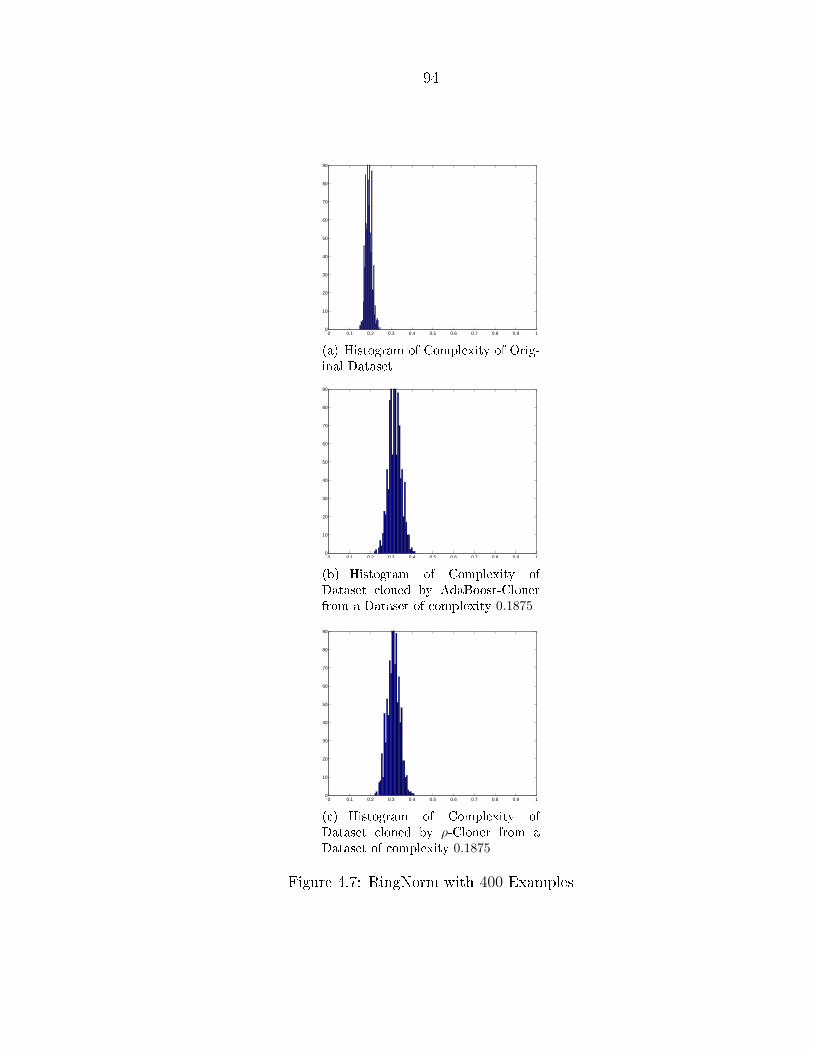
94
0 0.1 0.2 0.3 0.4 0.5 0.6 0.7 0.8 0.9 10
10
20
30
40
50
60
70
80
90
(a) Histogram of Complexity of Orig-inal Dataset
0 0.1 0.2 0.3 0.4 0.5 0.6 0.7 0.8 0.9 10
10
20
30
40
50
60
70
80
90
(b) Histogram of Complexity ofDataset cloned by AdaBoost-Clonerfrom a Dataset of complexity 0.1875
0 0.1 0.2 0.3 0.4 0.5 0.6 0.7 0.8 0.9 10
10
20
30
40
50
60
70
80
90
(c) Histogram of Complexity ofDataset cloned by ρ-Cloner from aDataset of complexity 0.1875
Figure 4.7: RingNorm with 400 Examples

95
0 0.1 0.2 0.3 0.4 0.5 0.6 0.7 0.8 0.9 10
10
20
30
40
50
60
70
80
90
(a) Histogram of Complexity of Orig-inal Dataset
0 0.1 0.2 0.3 0.4 0.5 0.6 0.7 0.8 0.9 10
10
20
30
40
50
60
70
80
90
(b) Histogram of Complexity ofDataset cloned by AdaBoost-Clonerfrom a Dataset of complexity 0.32
0 0.1 0.2 0.3 0.4 0.5 0.6 0.7 0.8 0.9 10
10
20
30
40
50
60
70
80
90
(c) Histogram of Complexity ofDataset cloned by ρ-Cloner from aDataset of complexity 0.32
Figure 4.8: RingNorm with 200 Examples
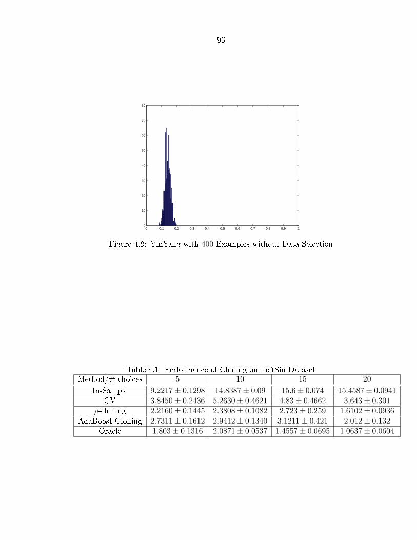
96
0 0.1 0.2 0.3 0.4 0.5 0.6 0.7 0.8 0.9 10
10
20
30
40
50
60
70
80
Figure 4.9: YinYang with 400 Examples without Data-Selection
Table 4.1: Performance of Cloning on LeftSin DatasetMethod/# choices 5 10 15 20
In-Sample 9.2217 ± 0.1298 14.8387 ± 0.09 15.6 ± 0.074 15.4587 ± 0.0941CV 3.8450 ± 0.2436 5.2630 ± 0.4621 4.83 ± 0.4662 3.643 ± 0.301
ρ-cloning 2.2160 ± 0.1445 2.3808 ± 0.1082 2.723 ± 0.259 1.6102 ± 0.0936AdaBoost-Cloning 2.7311 ± 0.1612 2.9412 ± 0.1340 3.1211 ± 0.421 2.012 ± 0.132
Oracle 1.803 ± 0.1316 2.0871 ± 0.0537 1.4557 ± 0.0695 1.0637 ± 0.0604

97
Table 4.2: Performance of Cloning on RingNorm DatasetMethod/# choices 5 10 15 20
In-Sample 2.3976 ± 0.0024 2.4836 ± 0.0018 2.4226 ± 0.002 2.5324 ± 0.0027CV 1.6166 ± 0.0122 1.7744 ± 0.0126 1.5580 ± 0.0089 1.7348 ± 0.0071
ρ-cloning 1.4540 ± 0.0133 1.6772 ± 0.0151 1.3112 ± 0.0095 1.3591 ± 0.0074AdaBoost-Cloning 1.4121 ± 0.021 1.6213 ± 0.0241 1.2336 ± 0.0067 1.2864 ± 0.0076
Oracle 1.1544 ± 0.009 1.1114 ± 0.0094 1.1101 ± 0.0063 1.0864 ± 0.0059
i.e., all choices available in the 5-model problem are available for selection in the 10-model problem, and are of increasing complexity. The 10-model problem contains allthe models in the 5-model problem, plus 5 additional models which are more powerful.
We can see a consistent improvement by using cloning over cross validation, andthe results are much closer to the Oracle approach, indicating that the cloned datasetsare of similar complexity and su�ciently independent from the original dataset. Thein-sample selection is consistently worsening as we increase the number of choices,which is expected. The cross-validation approach follows the same trend as the Oracleapproach, i.e., its bias decreases as the bias of the Oracle approach decreases. Thecloning approach, although not following the exact trend in the Oracle approach,gives results closer to the Oracle approach.
Table 4.2 summarizes the results of the 20-dimensional RingNorm dataset. Weobserve results similar to that of the LeftSin dataset, although the magnitude of errorshere is much smaller.
4.7.4 Cloning for Choosing a learning algorithm
Here we test the cloning approach in choosing between two learning algorithms. Weuse the same arti�cial datasets and use cloned datasets to select between two learningalgorithms. In an ideal setting, if we had access to the entire target function, we wouldthen choose the algorithm which would have a lower out-of-sample error upon learningfrom that dataset. We will use this concept as the baseline for comparison.
98
4.7.4.1 Experimental Setup
We use the Caltech Data Engine to generate di�erent target functions from variouslearning models. For each target, we generate a dataset of size 400. We can thenclone each dataset and get a cloned set of the same size. We train a 2− 5− 1 neuralnetwork and support vector classi�er on the original and cloned datasets, and reporthow often the performance on the cloned set matches the Oracle decision (which uses"illegal" information about the target function to choose a model). We also reportthe generalization performance of a system which uses the cloning process to decidewhich algorithm to use.
Given a target function f and a dataset S1, ..., SN generated from f , we generatethe cloners f c
1 , ..., fcN and cloned datasets Sc
1, ..., ScN . Given two learning algorithms
A1and A2 which map a dataset S to a hypothesis h = Ai(S) for i = 1, 2. De�neπij = e(Ai(Sj), f) and πij = e(Ai(S
cj ), f
cj ), as the out-of-sample performances of the
two models. We de�ne the hit-rate of a cloning process as
h =1
N
N∑
i=1
([πi1 < πi2] = [πci1 < πc
i2])
The hit-rate measures how often the decision of an algorithm on the cloned datasetmatches the actual Oracle decision. The hit-rate of the in-sample process can also besimilarly de�ned.
The performance of the Oracle chooser is de�ned as
Or =1
N
N∑
i=1
min (πi1, πi2)
and the performance of the cloner is de�ned as
Cln =1
N
N∑
i=1
(πi1[πci1 < πc
i2] + πi2[πci1 ≥ πc
i2])
A similar performance measure can be calculated for the selection which is donein-sample

99
IS =1
N
N∑
i=1
(πi1[νi1 < νi2] + πi2[νi1 ≥ νi2])
These quantities measure the overall performance of an algorithm which uses themethods to select a learning model. The Oracle method will have the lowest errormeasure, but it is not possible to implement that method.
4.7.4.2 Results
The cloning procedure was evaluated on 20 target functions generated using the dateengine from di�erent models. Figure 4.10 shows the hit-rates of the cloning methodagainst the in-sample selection. A random choice would give a hit-rate of 50%. Thecloning process has a higher hit-rate than the in-sample selection and is always betterthan random. Figure 4.11 summarizes the performance of the cloning process in termsof the average error obtained by choosing an algorithm based on the cloned dataset.There is a signi�cant improvement in the selection process by using the cloner overthe in-sample method.
4.8 Conclusion
We have presented a methodology to create cloned copies of datasets which caninherit the properties and structure of the original dataset, while minimizing thecontamination of the original dataset. We showed that the cloned datasets have asimilar complexity to the original datasets. We tested the cloning approach for thepurpose of model selection and choosing a learning algorithm. The experimentalresults indicate that the technique can be very useful in machine learning.
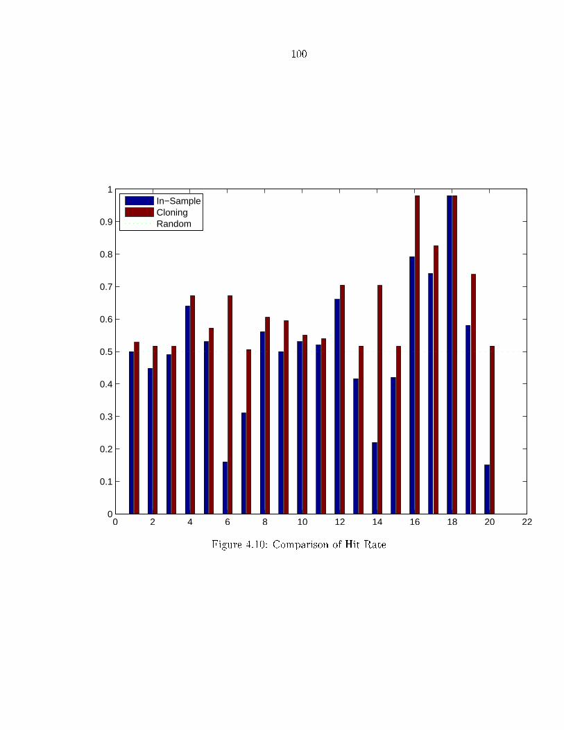
100
0 2 4 6 8 10 12 14 16 18 20 220
0.1
0.2
0.3
0.4
0.5
0.6
0.7
0.8
0.9
1
In−SampleCloningRandom
Figure 4.10: Comparison of Hit-Rate
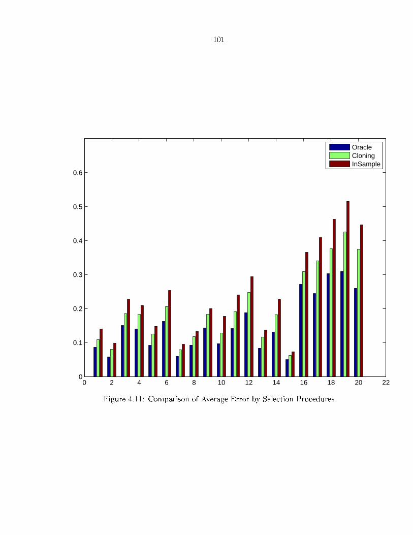
101
0 2 4 6 8 10 12 14 16 18 20 220
0.1
0.2
0.3
0.4
0.5
0.6
OracleCloningInSample
Figure 4.11: Comparison of Average Error by Selection Procedures

102
Bibliography
Y.S. Abu-Mostafa. Financial model calibration using consistency hints. IEEE Trans-actions on Neural Networks, 12(4):791�808, July 2001.
Y.S. Abu-Mostafa. Hints. Neural Computation, 7:639�671, 1995.
F. B. Baker. The Basics of Item Response Theory. Clearinghouse, 2001.
R.E. Barlow, D.J. Bartholomew, J.M. Bremner, and H.D. Brunk. Statistical InferenceUnder Order Restrictions. New York: Wiley, 1972.
C.L. Blake and C.J. Merz. UCI repository of machine learning databases, 1998. URLhttp://www.ics.uci.edu/∼mlearn/MLRepository.html.
B.E. Boser, I.M. Guyon, and V.N. Vapnik. A training algorithm for optimal marginclassi�ers. In Proceedings of the Fifth Annual Workshop on Computational LearningTheory, pages 144�152. ACM, 1992. ISBN 0-89791-497-X.
L. Breiman. Bagging predictors. Technical Report 421, Department of Statistics� Sep1994. URL ftp://ftp.stat.berkeley.edu/pub/users/breiman/bagging.ps.Z.
L. Breiman. Bias, variance, and arcing classi�ers. Techni-cal Report 460, Department of Statistics, Apr 1996. URLftp://ftp.stat.berkeley.edu/pub/users/breiman/arcall96.ps.Z.
L. Breiman. Arcing classi�ers. Annals of Statistic, 26(3):801�824, Jun 1998.
L. Breiman. Prediction games and arcing algorithms. Neural Computation, 11(7):1493�1517, Oct 1999.

103
H.D. Brunk. Maximum likelihood estimates of monotone parameters. The Annals ofMathematical Statistics, 26(4):607�616, Dec 1955.
H.D. Brunk. On the Estimation of Parameters Restricted by Inequalities. The Annalsof Mathematical Statistics, 29(2):437�454, June 1958.
D. Cohn, L. Atlas, and R. Ladner. Improving generalization with active learning.Machine Learning, 15(2):201�221, May 1994.
T.N. Cornsweet. The staircase method in psychophysics. American Journal of Psy-chology, 75:485�491, 1962.
C. Cox. Threshold dose-response models in toxicology. Biometrics, 43(3):511�23, Sep1987.
K. Deb, A. Pratap, S. Agarwal, and T. Meyarivan. A fast and elitist multiobjectivegenetic algorithm: NSGA-II. IEEE Transactions on Evolutionary Computation, 6(2):182�197, 2002. ISSN 1089-778X. doi: 10.1109/4235.996017.
A. Demiriz, K.P. Bennett, and J. Shawe-Taylor. Linear programming boosting viacolumn generation. Machine Learning, 46(1�3):225�254, 2002.
V.V. Fedorov. Theory of optimal experiments. Academic Press, 1972.
D.J. Finney. Probit Analysis. Cambridge University Press, 1971.
R. Fletcher and C.V Reeves. Function minimization by conjugate gradients. ComputerJournal, pages 149�154, 1964.
Y. Freund and R. E. Schapire. Experiments with a new boosting algorithm. InMachine Learning: Proceedings of the Thirteenth International Conference, pages148�156, 1996.
Y. Freund and R. E. Schapire. A decision-theoretic generalization of on-line learningand an application to boosting. In European Conference on Computational LearningTheory, pages 23�37, 1995.

104
A. J. Grove and D. Schuurmans. Boosting in the limit: Maximizing the margin oflearned ensembles. In AAAI/IAAI, pages 692�699, 1998.
G. Guo and H. Zhang. Boosting for fast face recognition. In Proc. IEEE ICCVWorkshop on Recognition, Analysis, and Tracking of Faces and Gestures in Real-Time Systems, 2001.
T. Hastie, R. Tibshirani, and J. Friedman. The Elements of Statistical Learning:Data Mining, Inference, and Prediction. Springer, 2001.
S. Klein. Measuring, estimating, and understanding the psychometric function: Acommentary. Perception and Psychophysics, 63(8):1421�1455, 2001.
R. Kohavi. A study of cross-validation and bootstrap for accuracy estimation andmodel selection. In Proceedings of the Fourteenth International Joint Conferenceon Arti�cial Intelligence, volume 2, pages 1137�1143. Morgan Kaufmann, 1995.
V. Koltchinskii and D. Panchenko. Empirical margin distributions and boundingthe generalization error of combined classi�ers. Annals of Statistics, 30(1):1�50,February 2002.
V. Koltchinskii, D. Panchenko, and F. Lozano. Bounding the generalization error ofconvex combinations of classiers: balancing the dimensionality and the margins,2000a.
V. Koltchinskii, D. Panchenko, and Fe. Lozano. Some new bounds on the generaliza-tion error of combined classi�ers. In NIPS, pages 245�251, 2000b.
M.R. Leek. Adaptive procedures in psychophysical research. Perception and Psy-chophysics, 63(8):1279�1292, November 2001.
L. Li. Data Complexity in Machine Learning and Novel Classi�cation Algorithms.PhD thesis, California Institute of Technology, Pasadena, CA, May 2006.

105
L. Li, Y.S. Abu-Mostafa, and A. Pratap. CGBoost: Conjugate gradi-ent in function space. Computer Science Technical Report CaltechC-STR:2003.007, California Institute of Technology, Pasadena, CA, Aug 2003. URLhttp://resolver.caltech.edu/CaltechCSTR:2003.007.
L. Li, A. Pratap, H.-T. Lin, and Y. S. Abu-Mostafa. Improving generalization bydata categorization. In A. Jorge, L. Torgo, P. Brazdil, R. Camacho, and J. Gama,editors, Knowledge Discovery in Databases: PKDD 2005, volume 3721 of LectureNotes in Arti�cial Intelligence, pages 157�168. Springer-Verlag, 2005. ISBN 3-540-29244-6.
F.M. Lord. Applications of item response theory to practical testing problems.Lawrence Erlbaum, 1980.
D.J.C. MacKay. Information-based objective functions for active data selection. Neu-ral Computation, 4:590�604, 1992.
O.L. Mangasarian and W.H. Wolberg. Cancer diagnosis via linear programming.SIAM Nesw, 23(5), September 1990.
L. Mason, P. L. Bartlett, and J. Baxter. Improved generalization through explicitoptimization of margins. Machine Learning, 38(3):243�255, Mar 2000a.
L. Mason, J. Baxter, P. Bartlett, and M. Frean. Boosting algorithms as gradientdescent. In S.A. Solla, T.K. Leen, and K.-R. Muller, editors, Advances in NeuralInformation Processing Systems 12, pages 512�518. MIT Press, 2000b.
S. Merler, B. Caprile, and C. Furlanello. Bias-variance control via hard points shaving.International Journal of Pattern Recognition and Arti�cial Intelligence, 18(5):891�903, 2004.
A. Nicholson. Generalization error estimates and training data valuation. PhD thesis,California Institute of Technology, Pasadena, CA, May 2002.

106
S.E. Palmer. Vision Science: Photons to Phenomenology. Bradford Books/MITPress, 1999.
A. Pentland. Maximum likelihood estimation: The best pest. Perception and Psy-chophysics, 28:377�379, 1980.
A. Pratap. Data Engine for Machine Learning Research. California Institute ofTechnology, 2003. URL http://www.work.caltech.edu/dengin.
J.O Ramsay. Monotone Regression Splines in Action. Statistical Science, 3(4):425�441, 1998.
R. B. Rao, D. Gordon, and W. Spears. For every generalization action is there reallyan equal and opposite reaction? analysis of the conservation law for generalizationperformance. In Proc. 12th International Conference on Machine Learning, pages471�479. Morgan Kaufmann, 1995.
L. Reyzin and R. E. Schapire. How boosting the margin can also boost classi�er com-plexity. In Proceedings of the 23rd International Conference on Machine Learning.ICML, 2006.
J. Rissanen. Modeling by shortest data description. Automatica, 14(5):465�471, 1978.
S. Salzberg. On comparing classi�ers: Pitfalls to avoid and a recommended approach.Data Mining and Knowledge Discovery, 1(3):317�328, 1997.
C. Scha�er. A conservation law for generalization performance. In Proceedings of theEleventh International Conference on Machine Learning, pages 259�265. MorganKaufmann, 1994.
R. E. Schapire and Y. Singer. Boostexter: A boosting-based system for text catego-rization. Machine Learning, 39(2/3):135�168, 2000.
R. E. Schapire, Yoav Freund, Peter Bartlett, andWee Sun Lee. Boosting the margin: anew explanation for the e�ectiveness of voting methods. In Proc. 14th InternationalConference on Machine Learning, pages 322�330. Morgan Kaufmann, 1997.

107
H Schwenk. Using boosting to improve a hybrid hmm/neural network speech recog-niser. In Proceedings of ICASSP'99, pages 1009�1012, 1999.
H. Schwenk and Y. Bengio. Adaboosting neural networks: Application to on-linecharacter recognition. In W. Gerstner, A. Germond, M. Hasler, and J.-D. Nicoud,editors, International Conference on Arti�cial Neural Networks, volume 1327 ofLecture Notes in Computer Science, pages 967�972. Springer, 1997.
G. Shakhnarovich. Statistical Data Cloning for Machine Learning. Master's thesis,Technion, 2001.
G. Shakhnarovich, R. El-Yaniv, and Y. Baram. Smoothed bootstrap and statisticaldata cloning for classi�er evaluation. In ICML '01: Proceedings of the EighteenthInternational Conference on Machine Learning, pages 521�528, San Francisco, CA,USA, 2001. Morgan Kaufmann Publishers Inc. ISBN 1-55860-778-1.
M.M. Taylor and C.D. Creelman. Pest: E�cient estimates on probability functions.The Journal of the Acoustical Society of America, 41(4A):782�787, April 1967.
V.N. Vapnik. The Nature of Statistical Learning Theory. Springer, 2000.
A.B. Watson. Probability summation over time. Vision Research, 19:515�522, 1971.
F.A. Wichmann and N.J. Hill. The psychometric function i: Fitting, sampling, andgoodness-of-�t. Perception and Psychophysics, 63:1293�1313, 2001.
D. H. Wolpert. The lack of a priori distinctions between learning algorithms. NeuralComputation, 8(7):1341�1390, Oct 1996.