Order of Convergence of Adaptive Step Algorithms for Ordinary

Differential Equations

Gideon Simpson

April 29, 2003

A paper submitted in partial fulfillment of

the requirements for the degree of

Bachelor of Arts

Cornell University

2003

Cornell University

Abstract

Order of Convergence of Adaptive Step Algorithms for

Ordinary Differential Equations

by Gideon Simspon

Faculty Supervisor:

Professor John Hubbard, Department of Mathematics

Faculty Advisor:

Professor Peter Kahn, Department of Mathematics

Adaptive, or Variable, Step Algorithms are frequently employed when solving differential equations.

For this paper, I studied the order of convergence of one such method, both experimentally and

analytically. In the course of this study, MATLAB was used for numerical computation and MAPLE

was used for symbolic computation. This paper suggests that, in neighborhoods where the second

derivative of the solution is zero, the order of convergence might be 3/2 for this variable step

algorithm.

1 Introduction

As many differential equations, even those as simple as x′ = x2 − t, lack analytic solutions, see [8],

numerical approximations are vital in applications. The computational procedures, from Euler’s

method to more advanced Runge-Kutta techniques, all involve iterative computations with greater

accuracy coming from additional iterations. Understanding the tradeoff between speed and accu-

racy in the computational work can be of tremendous importance in situations requiring the result

to be outputted in ”real-time”, such as might be required by aircraft guidance systems.

There are many numerical methods available. One-step methods use the data of a single point

in the space to calculate the next point; multi-step methods use a memory of several points to

determine how the solution travels. There are also explicit and implicit variants of both single

and multi step methods, explicit computing the iteration ”explicitly”, while implicit methods use

Newton’s Method to find the solution.

While all of these tools can be employed using a fixed step, the h in Euler’s method, the step

length can also be varied in hopes of improving the performance of the algorithm. In these modified

algorithms, the step size adjusts so that, ideally, small steps will be used in regions of high volatility

to retain precision while larger steps will be used in regions of low volatility to speed computation.

Indeed, this simple modification can offer significant improvements in speed.

The basic theme of all adaptive step methods is to measure this volatility by computing an

estimate of the local error at each iteration and comparing this estimate to a user defined error

tolerance. If it is above the tolerance, the computation is rejected, the stepsize made smaller,

and the solution and error estimate recomputed. If it is below the tolerance, the computation is

accepted, and the stepsize may be made larger. How one chooses to estimate local error and adjust

stepsize varies from algorithm to algorithm; stepsize selection in the widely used Runge-Kutta

algorithms are studied in [6] .

But what is the price of implementing an adaptive step length procedure inside a numerical

method? Intuitively, the parameter, tolerance, denoted τ or TOL, should be related to the global

error. How will the solutions converge as a function of τ? Are the solutions even guaranteed to

converge?

The methods in fact, do converge, under appropriate assumptions. In [12], an early text on the

subject, Stetter suggests that the global error of a variable step method ought to behave something

like

|u(t)− uτ (t)| = v(t)τ + o(τ), t ∈ [t0, tf ]

where the function v is independent of the tolerance, τ . In [11], Shampine shows that given an

Initial Value Problem,

x′ = f(t, x), x(t0) = x0

1

the global error can be bounded with the term

τeK(t−t0)

where K is the Lipschitz constant of f . This bound can be derived by modelling the global error

with the differential equation

ε′ = aε + τ, ε(t0) = 0

which has solution

ε(t) =τ

a(ea(t−t0) − 1)

This models the global error with a rate of change proportional to the error already in the system

and the new error introduced, which in variable step methods will be the tolerance.

In [13], using probabilistic and dynamical systems techniques, a bound of O(τ) on the error

is derived for error per unit step methods. This class of variable step algorithm will shortly be

explained, as it is the focus of this paper.

In [4], Gear adapts traditional methods for the asymptotic analysis of error in numerical methods

to variable step methods by defining a function step selection function hn = θ(tn)h where h is the

largest step size for the mesh {t0, t1, . . . tf}. Obviously, this function can only be defined a postieri.

This paper will seek to provide some analytic understanding of the order of convergence of basic

variable step method algorithms in actual equations. It studies an idealization of the variable step

algoirthm using Midpoint Euler, not used in practice. Section 2 will explain the Algorithm. Section

3 consists of data from numerical experiments with this algorithm. Additional data can be found

in Appendix A. Section 4 studies the differential equation

x′ = t2

and shows that the global error can behave like O(τ3/2). Much of the computation is done in

MATLAB with some symbolic computation handled by MAPLE.

2 The Algorithm

The algorithm is based upon that which appears in [2]. Similar material can be found in [1].

Given the initial value problem

x′ = f(t, x), x(t0) = x0

an initial step size h0, and a tolerance τ , compute the triple (tn+1, xn+1, hn+1) from (tn, xn, hn) as

follows:

Compute two different estimates of x(tn+1). Call them A1 and A2 and let A1 be computed

using one iteration of ordinary Euler’s method and let A2 be computed using two iterations of

2

Euler, each with step length hn/2. As would be expected, A2 will be more precise, so |A1−A2| is

a heuristic estimate of the local error in Euler. In this method, it is necessary to standardize this

error, and this is done in the obvious way of dividing the difference by hn, giving an estimate of the

error per unit step(EPUS). Other methods use the absolute error per step(EPS). A brief discussion

of these two methods, along with their counterparts employing extrapolation, can be found in [7].

Let

rn =|A1−A2|

hn(1)

denote the error per unit step. If rn > τ , reject the computation and the step size hn and replace

it with the following:

h′n =τ

rnhn (2)

In the case where the error per unit step exceeds the tolerance, (tn, xn, hn) 7−→ (tn, xn, h′n) and the

above computation is repeated with this new, smaller step size.

If rn does not exceed τ , take xn+1 = 2A2 −A1, tn+1 = tn + hn, and set hn+1 = τrn

hn, as in (2),

so

(tn, xn, hn) 7−→ (tn + hn, 2A2 −A1,τ

rnhn)

and the computation begins over again with this new triple.

This deserves some explanation. The assignment of 2A2 − A1 to xn+1 is an application of

Richardson extrapolation. Note that

2A2 −A1 = xn + hnf(tn +hn

2, xn +

hn

2f(tn, xn))

This is the Midpoint Euler solution to the IVP x′ = f , x(tn) = xn. Indeed, the solution computed

by the variable step method is the Midpoint Euler solution using the mesh {t0, t1, . . . , tf}.If (1) does not exceed the tolerance, then the ratio, τ/rn in 2 is obviously less than 1; multiplying

h by it will make h′ smaller than h and hopefully reduce the local error. Moreover, this ratio has

some theoretical basis. Let u denote the local solution such that u(tn) = xn. Via Taylor series

methods

A1 = xn + hnf(tn, xn) = u(tn) + hnu′(tn) = u(tn + hn) + Kh2n + O(h3

n)

Similarly, A2 can be expressed as

A2 = xn +hn

2f(tn, xn) +

hn

2f(tn +

hn

2, xn +

hn

2f(tn, xn)) = u(tn + hn) +

K

2h2

n + O(h3n)

With these representations,

rn ≈ 12Khn

3

Assume that K is constant in this neighborhood. Regardless of how rn compares to τ , if the

estimate of the local error, r, in the next iteration is to be close to τ , then h must be chosen such

that

K

2h ≈ τ

Using the approximation of K/2 = rn/hn, h must be such that

rn

hnh ≈ τ

or

h ≈ τ

rnhn

A few questions still remain. As defined, it is possible that tn + hn > tf in this algorithm. This

problem is avoided by defining

hn+1 = min{τ

rhn, tf − tn}

Another troublesome spot is when r = 0. This outcome can easily be generated by a constant

differential equation, x′ = c. This is remedied by letting hn+1 = tf − tn if r = 0.

Many variants also multiply (2) by a factor ρ < 1 to ensure that extra computation is avoided.

That is to say, if rn ≈ τ but perhaps slightly larger, it may be more efficient to accept the computed

values rather than redo this iteration. This is less of a concern in this study because the primary

concern is convergence, not computational speed. Also, note that the algorithm used in this paper,

varStep.m is only programmed to do forward integration, so t0 must be less than tf .

3 Numerical Data

A common question in numerical solutions to differential equations is what is the order of the global

error term. For a fixed step length h, methods usually converge like hp where p is an integer; p is

the order of the method of solution. Here, the primary parameter is τ , with the initial step size h0

a secondary parameter which will be fixed for much of the work in this paper. The focus will be

on the order of the global error as a function of τ . Throughout, roundoff error is assumed to be

negligible.

The equations that were studied were fairly elementary, including x′ = x and x′ = x2 sin t.

Three pieces of data were computed, the value at tf , the order of the error, and the number of

evaluations of the differential equation in the algorithm. The data was produced from MATLAB

using the programs studyFunc.m and VarStep.m included in Appendix C.

In these examples, an estimate of p, the order of the method, is computed by assuming that

the error term of the solution is of the form Kτp. Just as p is estimated under a fixed step method

in [8], the power of τ in the error term is computed with the formula

4

p ≈log

[u4τ (t)− u2τ (t)u2τ (t)− uτ (t)

]

log 2(3)

This is a local estimate of p in the sense that it is computed using only three datapoints, uτ (t),

u2τ (t), and u4τ (t). There are almost certainly higher order terms of τ in the error which will

influence the estimate of p.

As an initial example, consider x′ = x, with x(0) = 1. An initial step size of 1 was used

throughout. The columns indicate the tolerance, τ , the solution at t = 2, the local order of

convergence as computed using (3), and the number of evaluations of the differential equation, N ,

in the computation of the solution, one index of how much work the algorithm does to solve the

problem.

τ uτ (2) p N

2−1 6.466 0 10

2−2 6.71330966773715 0 20

2−3 7.2252980984118 -1.04979257210548 52

2−4 7.34963241424094 2.04188668018054 126

2−5 7.37940600864677 2.06211922403982 284

2−6 7.38666962423678 2.03527364242116 566

2−7 7.38846267343392 2.01827278038495 1100

2−8 7.38890813165467 2.00905303926358 2250

2−9 7.38901915611044 2.00441262917957 4492

2−10 7.3890468693087 2.00223237853353 9072

2−11 7.38905379227432 2.00111112733353 17930

2−12 7.38905552235882 2.00054768131583 36346

2−13 7.38905595479369 2.0002877527059 72306

2−14 7.38905606288597 2.0002192721944 143684

2−15 7.3890560898964 2.00067523124743 287416

This data seems fairly innocuous and suggests that the variable step algorithm might have the

same order of convergence as Midpoint Euler. The first two zeroes in the p column reflect that to

compute a local estimate of p as in (3), three successive values are needed.

However, the general behavior is not so good. Consider the simple IVP,

x′ = t2, x(−1) = −1/3 (4)

This is an elementary separable equation with the solution,

u(t) =t3

3

However, the data produced by the algorithm is not so easily understood.

5

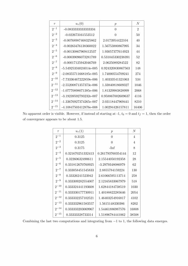
τ uτ (0) p N

2−1 -0.0833333333333334 0 2

2−2 -0.022673161553512 0 50

2−3 -0.00768987468325862 2.0173954422104 40

2−4 -0.00263476138360022 1.56753880867995 34

2−5 -0.00130867969412537 1.93057377614923 44

2−6 -0.00039096073281789 0.531045330238391 52

2−7 -0.00017125942046769 2.0625089284522 82

2−8 -5.54925334024014e-005 0.924320830867563 148

2−9 -2.08355711668185e-005 1.74000554709241 274

2−10 -7.73336467222859e-006 1.40333541321063 534

2−11 -2.55200871357373e-006 1.33840818609327 1046

2−12 -1.07770898071385e-006 1.81329983828999 2068

2−13 -3.19239592793232e-007 0.958867002609637 4116

2−14 -1.33676927374265e-007 2.03118447969441 8210

2−15 -4.10847503412876e-008 1.00294426157811 16406

No apparent order is visible. However, if instead of starting at -1, t0 = 0 and tf = 1, then the order

of convergence appears to be about 1.5.

τ uτ (1) p N

2−1 0.3125 0 4

2−2 0.3125 0 4

2−3 0.3175 -Inf 8

2−4 0.321670251332413 0.261793760354144 12

2−5 0.32260632490611 2.15544050192358 28

2−6 0.331812670760925 -3.2979348086979 62

2−7 0.333058451545833 2.8855784159224 130

2−8 0.33326241523942 2.61066595113714 258

2−9 0.333309282554007 2.12165833067979 518

2−10 0.333324441193608 1.62844184738519 1030

2−11 0.333330177730911 1.40188822285646 2054

2−12 0.333332257102521 1.46403254916817 4102

2−13 0.333332961583557 1.5615148330386 8202

2−14 0.333333203069967 1.54461886987576 16808

2−15 0.33333328733314 1.51896784441062 38508

Combining the last two computations and integrating from −1 to 1, the following data emerges.

6

τ uτ (1) p N

2−1 0.194727891156463 0 6

2−2 0.240646258503401 0 6

2−3 0.296053912702503 -0.271013941669279 44

2−4 0.323268901267306 1.02568385889969 50

2−5 0.326340705603548 3.14724320066697 64

2−6 0.3320144669392 -0.885219141445866 118

2−7 0.332274317832953 4.44854953928647 210

2−8 0.333133038390111 -1.72450470813989 404

2−9 0.333259447977653 2.76408284032707 786

2−10 0.333303102785096 1.53389344585764 1552

2−11 0.333325639755347 0.953846957606735 3088

2−12 0.33332838960669 3.03486804679354 6158

2−13 0.333332339976504 -0.522634089082801 12308

2−14 0.333332435129221 5.3755990531086 24990

2−15 0.333333186970961 -2.98211225297333 54600

Finally, staying away from zero, 2nd order behavior emerges

τ uτ (−.2) p N

2−1 -0.0833333333333334 0 2

2−2 -0.0202366534145525 0 50

2−3 -0.00740806430154643 2.29820158241225 38

2−4 -0.00459732183066538 2.19033933108909 32

2−5 -0.00332018385481633 1.13803688018961 42

2−6 -0.00286879030452648 1.50045668537265 48

2−7 -0.0027233345065876 1.63380500070324 78

2−8 -0.00268329738773555 1.86117074019428 140

2−9 -0.0026712015335355 1.7268255038578 260

2−10 -0.00266785820741691 1.8551566629858 508

2−11 -0.00266697364535809 1.91824881913785 1000

2−12 -0.0026667451187649 1.95260130391113 1980

2−13 -0.00266668639873723 1.96043750569122 3946

2−14 -0.0026666716150992 1.98985130951448 7876

2−15 -0.00266666790578401 1.99477656832753 15742

Note that the solution to this problem, u(t) = t3/3, has an inflection point, a point where the 2nd

derivative is 0, at 0.

Nor does this appear to be a behavior that is suppressed when tf gets away from 0. Consider

7

the same problem again, but this time with t0 = 0 and tf = 5. An order of convergence of 1.5 once

again emerges.

τ uτ (5) p N

2−1 41.5322962114305 0 52

2−2 41.5682959214522 0 96

2−3 41.5792663304294 1.71436797519626 192

2−4 41.6541075090578 -2.77021496841868 398

2−5 41.6643686135613 2.86664624814561 802

2−6 41.6660748038678 2.58833555344446 1602

2−7 41.6664681457328 2.11692292067944 3202

2−8 41.6665940013819 1.64401377209014 6406

2−9 41.6666410400539 1.41985073870365 12820

2−10 41.6666579614173 1.47500151215128 28644

2−11 41.66666366881 1.5679420772305 63640

2−12 41.6666656185689 1.54953612817455 133828

2−13 41.6666662971135 1.52278013814601 274826

2−14 41.6666665340111 1.5181803942742 553018

2−15 41.6666666191413 1.47651896433204 1032332

This data, along with that found in Appendix A, suggests that different behaviors can emerge

depending on whether or not the solution has an inflection point in the interval [t0, tf ]. These

observations give rise to the following conjecture,

Conjecture 3.0.1 Given an IVP, x′ = f(t, x), x(t0) = x0. If u is a solution and in (t0, tf ], there

exists t such that u′′(t) = 0, then, the sequence of local estimates of p, computed with (3), does not

converge as τ → 0 in the variable step algorithm.

If no such t exists, but u′′(t0) = 0, the sequence of local estimates of p converge to 32 .

If u′′(t) 6= 0, for any t ∈ [t0, tf ], then the sequence converges to 2.

Intuitively, in neighborhoods of a solution containing an inflection point, the solution will be

approximately affine. Computational work could be curtailed near such points, as relatively larger

steps can be taken. It would thus be expected that the algorithm would behave differently in such

neighborhoods. That it behaves as the data suggests is highly unexpected.

4 Analysis and Results

4.1 Statistics

Some of these experiments, in particular those with an inflection point in the interior of the interval

of integration, suggest that the error might be independent of the tolerance. However, things are

8

not quite so dismal. If, instead of computing estimates of the local p value, p is estimated using an

ordinary least squares regression of log(|u(tf )− uτ (tf )|) against log(τ), a different picture emerges.

This analysis was only conducted for problems in which an analytic solution, u, exists.

For the equation log(|u(tf )− uτ (tf )|) = a0 + a1 log(τ), the following values of a0 and a1 were

computed for the prior equations, along with the Pearson correlation coefficients of the relationship

between the variables.

IVP a0 a1 r

x′ = x2 sin(t), x(0) = .3, tf = π -0.550150586587259 1.33545071201549 0.96520235972456

x′ = cos(t), x(0) = 0, tf = π/2 -0.65422291831959 1.52350573342793 0.990152825801733

x′ = t2, x(−1) = −1/3, tf = 0 -1.67881433394 1.46450645607541 0.999682037631776

x′ = t2, x(−1) = −1/3, tf = 1 -0.440717503125832 1.44195269912236 0.997392304176616

Each of these regressions used the 15 data points that appear elsewhere in this paper. This data,

in contrast to the locally computed estimates, suggests that a relationship of the form

u(tf ) ≈ uτ (tf ) + Kτ32

might exist in certain cases. Augmenting Conjecture 3.0.1, the following is conjectured,

Conjecture 4.1.1 Under appropriate conditions, if the solution to x′ = f(t, x) has an inflection

point in the region [t0, t], then the variable step method converges like

|u(t)− uτ (t)| ≤ Kτ32 + O(τ q) (5)

where q > 3/2.

This can be shown analytically for x′ = t2, if assumptions about the mesh produced by the

algorithm are made in order to simplify computation.

4.2 Mesh Assumptions

Conjecture 4.2.1 Given a tolerance τ , let

N =⌈

14τ

⌉(6)

Then for the IVP x′ = t2 and x(t0) = x0, tf , where t0 and tf are integers, the mesh t0, t1, . . . such

that

∣∣t2i − t2i+1

∣∣ = 1/N (7)

approximates the mesh produced by the variable step algorithm.

9

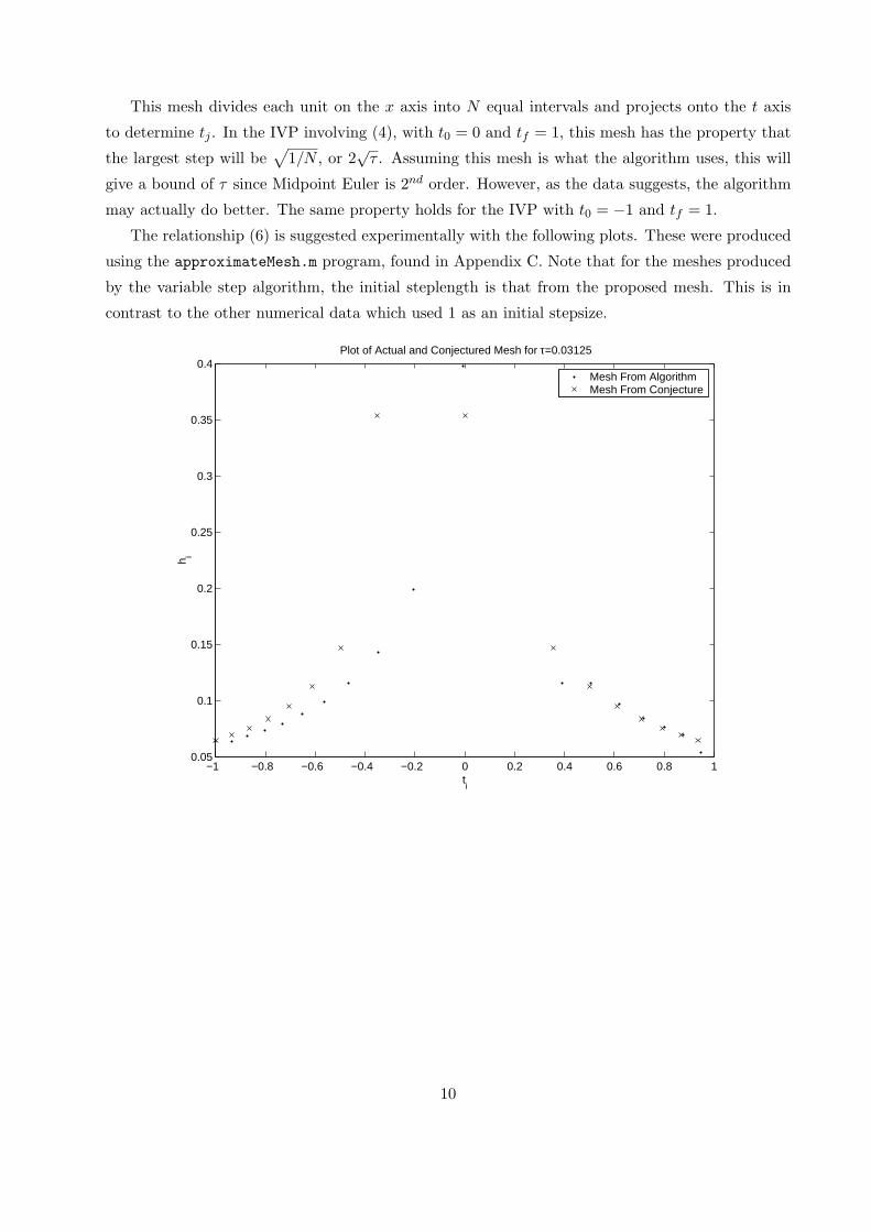
This mesh divides each unit on the x axis into N equal intervals and projects onto the t axis

to determine tj . In the IVP involving (4), with t0 = 0 and tf = 1, this mesh has the property that

the largest step will be√

1/N , or 2√

τ . Assuming this mesh is what the algorithm uses, this will

give a bound of τ since Midpoint Euler is 2nd order. However, as the data suggests, the algorithm

may actually do better. The same property holds for the IVP with t0 = −1 and tf = 1.

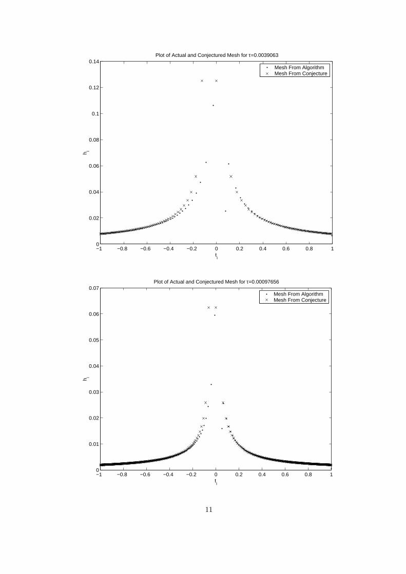
The relationship (6) is suggested experimentally with the following plots. These were produced

using the approximateMesh.m program, found in Appendix C. Note that for the meshes produced

by the variable step algorithm, the initial steplength is that from the proposed mesh. This is in

contrast to the other numerical data which used 1 as an initial stepsize.

−1 −0.8 −0.6 −0.4 −0.2 0 0.2 0.4 0.6 0.8 10.05

0.1

0.15

0.2

0.25

0.3

0.35

0.4Plot of Actual and Conjectured Mesh for τ=0.03125

ti

h i

Mesh From AlgorithmMesh From Conjecture

10

−1 −0.8 −0.6 −0.4 −0.2 0 0.2 0.4 0.6 0.8 10

0.02

0.04

0.06

0.08

0.1

0.12

0.14Plot of Actual and Conjectured Mesh for τ=0.0039063

ti

h i

Mesh From AlgorithmMesh From Conjecture

−1 −0.8 −0.6 −0.4 −0.2 0 0.2 0.4 0.6 0.8 10

0.01

0.02

0.03

0.04

0.05

0.06

0.07Plot of Actual and Conjectured Mesh for τ=0.00097656

ti

h i

Mesh From AlgorithmMesh From Conjecture

11

−1 −0.8 −0.6 −0.4 −0.2 0 0.2 0.4 0.6 0.8 1

2

4

6

8

10

12x 10

−3 Plot of Actual and Conjectured Mesh for τ=3.0518e−005

ti

h i

Mesh From AlgorithmMesh From Conjecture

4.3 Error Behavior

Assuming the mesh is as defined in the previous section, to solve x′ = t2 from −1 to 0, with

u(0) = −1/3, the variable step algorithm would compute the sum

uτ (0) =N−1∑

i=0

(

√1− i

N−

√1− i + 1

N)14

(√1− i + 1

N+

√1− i

N

)2

− 1/3

This can be computed symbolically using MAPLE. In the computations, it is necessary to break

up the sum in order to use the series command properly.

> t:=k->-sqrt(1-k/N);

t := k → −√

1− k

N> h:=k->t(k+1)-t(k);

h := k → t(k + 1)− t(k)> sum(h(k)*(t(k)+h(k)/2)^2,k=0..N-3)+h(N-2)*(t(N-2)+h(N-2)/2)^2+h(N-1)*> (t(N-1)+h(N-1)/2)^2-1/3;

12

(N−3∑

k=0

(−√

1− k + 1N

+

√1− k

N) (−1

2

√1− k

N− 1

2

√1− k + 1

N)2)

+ (−√

1− N − 1N

+

√1− N − 2

N) (−1

2

√1− N − 2

N− 1

2

√1− N − 1

N)2

+14

(1− N − 1N

)(3/2) − 13

> asympt(%,N);

O((1N

)(3/2))

Substituting the relation N ≈ 14τ into this gives

uτ (0) = O(τ32 ) (8)

Similarly, if asked to compute the symbolic representation of the implied sum from 0 to 1,

MAPLE generates

> t:=k->sqrt(k/N);

t := k →√

k

N> h:=k->t(k+1)-t(k);

h := k → t(k + 1)− t(k)

> sum(h(k)*(t(k)+h(k)/2)^2,k=1..N-1)+h(0)*(t(0)+h(0)/2)^2;

(N−1∑

k=1

(

√k + 1

N−

√k

N) (

12

√k

N+

12

√k + 1

N)2)

+

14

√1N

N

> asympt(%,N);

13

+ O((1N

)(3/2))

Obviously, if N ≈ 14τ , then

uτ (1) =N−1∑

i=0

(

√i + 1N

−√

i

N)14

(√i

N+

√i + 1N

)2

=13

+ O(τ32 ) (9)

If instead, the equation were considered as the integral from 1 to 2, MAPLE calculates that

> t:=k->sqrt(k/N);

t := k →√

k

N> h:=k->t(k+1)-t(k);

h := k → t(k + 1)− t(k)

> sum(h(k)*(t(k)+h(k)/2)^2,k=N..4*N-1)+1/3;

13

(4 N−1∑

k=N

(

√k + 1

N−

√k

N) (

12

√k

N+

12

√k + 1

N)2)

+13

> simplify(asympt(%,N));

1122880

327680N4 − 1280N2 + 31 + 122880O(1

N5) N4

N4

This simplifies to

83

+ O(1/(N2))

Using the relation between N and τ , this gives

83

+ O(τ2)

a 2nd order solution, as desired.

Symbolic computations in MAPLE were further able to show that the error will be 2nd order

for t0 > 0 and tf > t0 for (4), a region where the solution contains no inflection points, using the

assume command. These computations can be found in the Appendix B.

Moreover, it is true in general that if the true solution, u to the differential equation x′ = f(t, x)

has no inflection points in the region, then the variable step algorithm converges as Kτ2 + O(τ3).

Theorem 4.3.1 Let x′ = f(t, x), x(t0) = x0 be an IVP such that f is continuously differentiable

and in a neighborhood of the graph (t, u(t)), u′′ is bounded away from zero

∣∣u′′∣∣ =∣∣∣∣∂f

∂t+

∂f

∂xf

∣∣∣∣ ≥ L > 0

then uτ , the variable step algorithm solution, will converge to u as Kτ2 + O(τ3).

This can be proved as follows

If A1 = xi + hif(ti, xi) and A2 = xi + hi/2f(ti, xi) + hi/2f(ti + hi/2, xi + hi/2f(ti, xi), and

r = |A2−A1|, then

r =12|f(ti + hi/2, xi + hi/2f(ti, xi)− f(ti, xi))|

And the step is accepted if r < τ .

Using the Mean Value Theorem,

f(ti + hi/2, xi + hi/2f(ti, xi))− f(ti, xi) =(

∂f

∂t+

∂f

∂xf |(t∗,x∗)

)hi/2

under the assumption that (ti, xi) is in the neighborhood U of the graph (t, u(t)) such that

u′′ 6= 0. Now,

r ≥ L

4hi

14

thus the next step produced by the algorithm will be

hi+1 =τ

rhi ≤ 4

τ

L

This actually implies that the maximum possible step size in the mesh will be 4 τL . Suppose h0

exceeded this limit. Then the estimate of the local error for x1 would be∣∣∣∣∂f

∂t+

∂f

∂xf |(t∗,x∗)

∣∣∣∣h0

4≥ L

h0

4> τ

Therefore h0 < 4 τL , and inductively, all hi are likewise bounded.

Now it is neccessary to show that

|u(t)− uτ (t)| ≤ Kτ2 + O(τ3)

for all t ∈ [t0, tf ]. As in [8], define the solution using quadratic interpolation between the meshpoints

as follows

uτ (t) = xi + f(ti, xi)(t− ti) + α(t− ti)2

where

α = [f(ti + hi/2, xi + hi/2f(ti, xi))− f(ti, xi)] /hi

uτ is thus the variable step solution with quadratic interpolation.

u′τ (t)− f(t, uτ (t)) = Ahi(t− ti) + B(t− ti)2 + O((t− ti)3)

Since t− ti ≤ hi,

∣∣u′τ (t)− f(t, uτ (t))∣∣ ≤ Kh2

i + O(h3i ) (10)

But since hi ≤ 4 τL ,

∣∣u′τ (t)− f(t, uτ (t))∣∣ ≤ 16K

Lτ2 + O(τ3) (11)

With an application of the Fundamental Inequality to (11), uτ is 2nd order. Details of the con-

stant K, can be found in Appendix B, where 2nd order convergence is proved for the quadratic

interpolation of Midpoint Euler.

The results computed for (8) and (9) were dependent on the mesh assumption. This begs the

question of how good an assumption it is. The difference between the approximate mesh given by

(7) and the actual mesh can be derived analytically using MAPLE. The following computations are

for the mesh approximation from 0 to 1. Given τ , assume it is sufficiently small such that 14τ > 1.

Moreover, assume it is an integer for simplicity.

N =14τ

15

Let t0 and h0 = 2√

τ . Let hk denote the stepsize produced by the algorithm and hk denote the

proposed stepsize. Assume

hk = hk

for some k ≥ 0. Also assume that

tk =√

k/N = 2√

kτ

If hk+1 is computed as in (1) and (2), as in the variable step algorithm, then the difference between

hk+1 and hk can be computed symbolically to be

hk+1 = hk+1 +58√

τ1

k3/2− 53

64√

τ1

k5/2+ O(

1k7/2

) (12)

where hk+1 is the step size proposed by this approximation. So the error disappears quite rapidly

when computing with the approximate mesh from t = 0 to t = 1 for the test equation x′ = t2 and

details of this MAPLE computation can be found in Appendix B.

5 Remarks

Attempts to show that the global error, taking into account the discrepancy between the actual

and approximate mesh, is of order 3/2 near the inflection point at 0 were unsuccessful, even in the

specific case of x′ = t2 . These attempts involved incorporating the asymptotic error of (12) into

the sum. Let εk+1 be the error from (12), since this was the difference between the two different

k + 1-th steps. Also, assume that ε0 = 0 since h0 = h0.

hk = hk + εk

tk =k−1∑

j=0

hj =k−1∑

j=1

hj + εj

Since the hj =√

j+1N −

√jN , this sum telescopes to

tk =

√k

N+

k−1∑

j=1

εj

Steps can then be defined as

hk = tk+1 − tk

With these expressions, MAPLE might have been able to the simplify the Midpoint Euler sum

into something recognizable. Unfortunately, it could not.

> t_est:=k->2*sqrt(k*TOL);

16

t est := k → 2√

k TOL> err:=k->5/8*sqrt(TOL)*(1/k)^(3/2)-53/64*sqrt(TOL)*(1/k)^(5/2)+587/512> *sqrt(TOL)*(1/k)^(7/2)-6877/4096*sqrt(TOL)*(1/k)^(9/2);

err := k →58

√TOL (

1k)(3/2) − 53

64

√TOL (

1k)(5/2) +

587512

√TOL (

1k)(7/2) − 6877

4096

√TOL (

1k)(9/2)

> t_corrected:=k->t_est(k)+sum(err(j),j=1..k-1);

t corrected := k → t est(k) + (k−1∑

j=1

err(j))

> h_corrected:=k->t_corrected(k+1)-t_corrected(k);

h corrected := k → t corrected(k + 1)− t corrected(k)> sum(h_corrected(k)*( t_corrected(k)+h_corrected(k+1)/2)^2> ,k=1..1/(4*TOL)-1)+2*sqrt(TOL)*4*TOL;

17

1/41

TOL−1

∑

k=1

2

√(k + 1)TOL +

k∑

j=1

(58

√TOL (

1j)(3/2) − 53

64

√TOL (

1j)(5/2) +

587512

√TOL (

1j)(7/2) − 6877

4096

√TOL (

1j)(9/2))

− 2√

k TOL−

k−1∑

j=1

(58

√TOL (

1j)(3/2) − 53

64

√TOL (

1j)(5/2) +

587512

√TOL (

1j)(7/2) − 6877

4096

√TOL (

1j)(9/2))

2√

k TOL +

k−1∑

j=1

(58

√TOL (

1j)(3/2) − 53

64

√TOL (

1j)(5/2) +

587512

√TOL (

1j)(7/2) − 6877

4096

√TOL (

1j)(9/2))

+√

(k + 2)TOL +12

k+1∑

j=1

(58

√TOL (

1j)(3/2) − 53

64

√TOL (

1j)(5/2) +

587512

√TOL (

1j)(7/2) − 6877

4096

√TOL (

1j)(9/2))

−√

(k + 1)TOL− 12

k∑

j=1

(58

√TOL (

1j)(3/2) − 53

64

√TOL (

1j)(5/2) +

587512

√TOL (

1j)(7/2) − 6877

4096

√TOL (

1j)(9/2))

2

+ 8TOL(3/2)

> series(%,TOL=0);

Error, (in series/int) invalid arguments

Perhaps a true asymptotic expansion can be found through more trickery with MAPLE. Some

was needed to generate the results in this paper, such as manually splitting sums. Such work is

further discussed in [3]. Additional effor might also derive the constants in front of the τ3/2 term,

which MAPLE would not output, giving only O(τ3/2).

Frequently, the adaptive step algorithms include restrictions that prevent step sizes from in-

creasing too rapidly, or beyond a certain bound. Suppose the maximal step size in the algorithm

18

is limited to some

ατ q

Using the exact same computations as in the proof of 4.3.1, particularly (10), since hi ≤ ατ q,

∣∣u′τ (t)− f(t, uτ (t))∣∣ ≤ Mτ2q + O(τ3q)

Lastly, although it was not encountered in any computations for this paper, it is possible that

the variable step algorithm used here might encounter a Zeno’s Paradox situation. That is to say,

it might enter into a situation in which it will successfully take a step and multiply it by a factor

close to 1, then have to make the step half as large, taking a step and multiplying it by a factor

close to 1, and then having to shrink it in half again. This situation is frequently avoided in codes

in practice by putting in some sort of an hmin into the algorithm, preventing the steps from getting

any smaller. This specific problem is highlighted in [9].

19

A Numerical Computations

The numerical data in this paper was computed using a MATLAB Release 12 Student Version on a

Microsoft Windows XP Home machine. Functions were defined using inline definitions, for example

f=inline(’t^2’,’t’,’x’);

defines the differential equation x′ = t2. The function studyFunc.m, which was the primary tool of

computation was used as follows

EDU>> data=studyFunc(f,[-1,0],-1/3,1,15);

-0.0833333333333334 0 2

-0.022673161553512 0 50

-0.00768987468325862 2.0173954422104 40

-0.00263476138360022 1.56753880867995 34

-0.00130867969412537 1.93057377614923 44

-0.00039096073281789 0.531045330238391 52

-0.00017125942046769 2.0625089284522 82

-5.54925334024014e-005 0.924320830867563 148

-2.08355711668185e-005 1.74000554709241 274

-7.73336467222859e-006 1.40333541321063 534

-2.55200871357373e-006 1.33840818609327 1046

-1.07770898071385e-006 1.81329983828999 2068

-3.19239592793232e-007 0.958867002609637 4116

-1.33676927374265e-007 2.03118447969441 8210

-4.10847503412876e-008 1.00294426157811 16406

The statistical data was calculated by the following commands

EDU>> X=[ones(15,1),log(2.^-(1:15))’] X =

1 -0.693147180559945

1 -1.38629436111989

1 -2.07944154167984

1 -2.77258872223978

1 -3.46573590279973

1 -4.15888308335967

1 -4.85203026391962

1 -5.54517744447956

1 -6.23832462503951

1 -6.93147180559945

20

1 -7.6246189861594

1 -8.31776616671934

1 -9.01091334727929

1 -9.70406052783923

1 -10.3972077083992

EDU>> y=log(\abs(data(:,2)-0)); EDU>> X\y ans =

-1.67881433394

1.46450645607541

EDU>> corrcoef(log(2.^-(1:15))’,y) ans =

1 0.999682037631776

0.999682037631776 1

It was in the examination of x′ = x2 sin(t) with x(0) = .3, for which data was available in [8],

that strange behavior in the local estimates of p was first encountered. An initial step size of 1 is

used.

τ x(π) p N

2−1 0.722458967757504 0 4

2−2 0.722458967757504 0 4

2−3 0.722458967757504 NaN 4

2−4 0.722458967757504 NaN 4

2−5 0.717896563579454 -Inf 58

2−6 0.735858750406221 -1.97709683922223 88

2−7 0.746563097779752 0.746766163653791 156

2−8 0.74933391606463 1.94981283509519 262

2−9 0.749859488623444 2.39835024268101 416

2−10 0.750018907012542 1.72107189617294 764

2−11 0.750009436858396 4.07328633663428 1378

2−12 0.750011796984316 2.00452407459759 2638

2−13 0.750002663890777 -1.95223977504548 5096

2−14 0.750001198470168 2.63978879811532 9842

2−15 0.750000264892773 0.650473277570399 20624

The local estimates of p do not appear to converge at all. Note that there is a point of inflection

near 2.116648. This is found by solving the problem analytically, which has solution

x(t) =1

cos t + 10/3

and finding the zeros of the second derivative.

Suppose instead that this is computed only to t = 2.1 with other parameters held constant.

21

τ uτ (2.1) p N

2−1 0.51704387450231 0 4

2−2 0.51704387450231 0 4

2−3 0.51704387450231 NaN 4

2−4 0.51704387450231 NaN 4

2−5 0.51704387450231 NaN 4

2−6 0.536323153250487 -Inf 76

2−7 0.544271805734701 1.27826887066196 122

2−8 0.546253692335937 2.00383588717288 194

2−9 0.54673927685961 2.02908007083514 274

2−10 0.54686002360769 2.00773810611921 486

2−11 0.546890150376933 2.00286646175888 818

2−12 0.546897675999645 2.00116309992646 1520

2−13 0.546899556586011 2.00062839960012 2836

2−14 0.546900026391271 2.00104779220287 5240

2−15 0.546900143848657 1.99992543513437 10642

Now suppose we go a bit farther, to t = 2.4.

τ uτ (2.4) p N

2−1 0.579389455077842 0 4

2−2 0.579389455077842 0 4

2−3 0.579389455077842 NaN 4

2−4 0.579389455077842 NaN 4

2−5 0.58488070598879 -Inf 60

2−6 0.612549574326837 -2.33305689989366 78

2−7 0.623330441106537 1.35979046348554 124

2−8 0.625828788698946 2.10942705853882 198

2−9 0.626458818888622 1.98748134532802 280

2−10 0.626582065811644 2.3538693322893 494

2−11 0.626594247535269 3.33876144526631 834

2−12 0.62659767205183 1.83074603610992 1552

2−13 0.626591831755468 -0.770141242189163 2906

2−14 0.62659091669334 2.67409997569969 5380

2−15 0.626590296079336 0.56017344580703 10916

Setting t0 = 2.4 and letting x0 = 1cos 2.4+10/3 , the 2nd convergence reappears.

22

τ uτ (π) p N

2−1 0.430558407286946 0 2

2−2 0.430558407286946 0 2

2−3 0.430558407286946 NaN 2

2−4 0.430558407286946 NaN 2

2−5 0.430558407286946 NaN 2

2−6 0.430968469017373 -Inf 6

2−7 0.429092394892747 -2.19380381701507 14

2−8 0.428717102013108 2.32162800696695 26

2−9 0.428614478582528 1.87065675946432 50

2−10 0.428583383312818 1.72259312320438 102

2−11 0.428574582238823 1.82094363906137 206

2−12 0.42857223787692 1.90848428870009 410

2−13 0.428571633495286 1.95566357212922 822

2−14 0.428571480124957 1.97844041544309 1650

2−15 0.428571441499965 1.98941287271258 3374

Considering x′ = cos t, with x(0) = 0 and h0 = 1,

τ uτ (π/2) p N

2−1 1.03828429211418 0 4

2−2 1.03828429211418 0 4

2−3 1.03813595180218 -Inf 8

2−4 1.03659449544613 -3.37731142868838 12

2−5 1.00594241635709 -4.3136189858245 34

2−6 1.00105697179672 2.64942317921257 66

2−7 1.00026693488638 2.62849788661184 134

2−8 1.00009081369474 2.1653515465401 262

2−9 1.00003414473226 1.63593781644774 518

2−10 1.00001231493431 1.37626001164815 1030

2−11 1.00000423622959 1.43410287217546 2066

2−12 1.00000146914696 1.54575827514331 4140

2−13 1.0000005166823 1.53862824592483 8544

2−14 1.00000018272698 1.51201050079089 18666

2−15 1.00000006567597 1.51251762722556 41540

This has an inflection point at 0; note that the local p values look like 1.5. Again, avoiding the

inflection point results in the now expected 2nd order convergence. Starting at .1, with x0 = sin .1

the following output is produced

23

τ uτ (π/2) p N

2−1 1.03497294673354 0 4

2−2 1.03497294673354 0 4

2−3 1.03497294673354 NaN 4

2−4 1.01561542133705 -Inf 14

2−5 1.00272905447993 0.587048962928639 34

2−6 1.00064812850422 2.63054802155216 66

2−7 1.00020191336495 2.22141427778827 130

2−8 1.00006583157955 1.7132654879343 254

2−9 1.00001968285354 1.56011124852146 510

2−10 1.00000537159494 1.68914026566336 1018

2−11 1.00000139340514 1.84696654091949 2044

2−12 1.00000035375421 1.93601289741658 4120

2−13 1.00000008903624 1.97357112485259 8516

2−14 1.00000002232824 1.98852451248958 18588

2−15 1.0000000055906 1.99476389525267 41234

B Symbolic Computations

The symbolic data in this paper was computed using a MAPLE 7 Student Version on a Microsoft

Windows XP Home machine. Although it does not tackle the problems confronted in this paper, [3]

gives examples on the use of MAPLE for studying numerical methods symbolically. In particular

it derives Runge-Kutta formulas.

B.1 Error of Approximate Mesh

> h_est:=k->2*sqrt((k+1)*TOL)-2*sqrt(k*TOL);

h est := k → 2√

(k + 1)TOL− 2√

k TOL

> t_est:=k->2*sqrt(k*TOL);

t est := k → 2√

k TOL

> A1:=x_k+h_est(k) *(t_est(k))^2;

A1 := x k + 4 (2√

(k + 1)TOL− 2√

k TOL) k TOL> A2:=x_k+h_est(k)/2*(t_est(k))^2+h_est(k)/2> * (t_est(k)+h_est(k)/2)^2;

A2 := x k + 2 (2√

(k + 1)TOL− 2√

k TOL) k TOL

+12

(2√

(k + 1)TOL− 2√

k TOL) (√

k TOL +√

(k + 1)TOL)2

> r:=(A2-A1)/h_est(k);

24

r :=−2%1 k TOL +

12

%1 (√

k TOL +√

(k + 1)TOL)2

%1%1 := 2

√(k + 1)TOL− 2

√k TOL

> h_algorithm:=TOL/r * h_est(k);

h algorithm :=TOL%12

−2 %1 k TOL +12

%1 (√

k TOL +√

(k + 1)TOL)2

%1 := 2√

(k + 1)TOL− 2√

k TOL> simplify(%);

4(√

(k + 1)TOL−√

k TOL)TOL−2 k TOL + 2

√k TOL

√(k + 1)TOL + TOL

> h_approx:=h_est(k+1);

h approx := 2√

(k + 2)TOL− 2√

(k + 1)TOL

> series(h_algorithm-h_approx,TOL=0); (2

√k + 1− 2

√k)2

−2 (2√

k + 1− 2√

k) k +12

(2√

k + 1− 2√

k) (√

k +√

k + 1)2− 2

√k + 2 + 2

√k + 1

√

TOL

> asympt(%,k);

58

√TOL (

1k)(3/2) − 53

64

√TOL (

1k)(5/2) +

587512

√TOL (

1k)(7/2) − 6877

4096

√TOL (

1k)(9/2)

+ O((1k)(11/2))

B.2 Proof of Order of Convergence of x′ = t2 with 0 < t0 < tf

Using the mesh approximation for solving (4) in which f(ti+1, xi+1) − f(ti, xi) is constant and

proportional to the tolerance, it can be shown that if tf > t0 > 0, then the variable step algorithm

should exhibit 2nd order convergence.

> assume(t0>0,tf>t0);

> t:=k->sqrt(t0^2+k/N);

t := k →√

t0 2 +k

N> h:=k->t(k+1)-t(k);

h := k → t(k + 1)− t(k)

> sum(h(k)*(t(k)+h(k)/2)^2,k=0..((tf^2-t0^2)*N-1))+x0;

(tf ˜2−t0˜2) N−1∑

k=0

(

√t0˜2 +

k + 1N

−√

t0˜2 +k

N) (

12

√t0˜2 +

k

N+

12

√t0˜2 +

k + 1N

)2

+ x0

25

> asympt(%,N,4);

−16

(t0˜2)(3/2) − 16

t0˜3 +16

(tf ˜2)(3/2) +16

tf ˜3 − 12

%4%32 +12

%2%12 + x0 +

(14

tf ˜

− 14

%4%3tf ˜

− 14

%32

tf ˜+

112

(12

1tf ˜

− 12

1√tf ˜2

)%32 +16

%4%3

1

41√tf ˜2

+

14

tf ˜

− 14

t0˜ +

14

%2%1

t0˜+

14

%12

t0˜− 1

12(12

1t0˜

− 12

1√t0˜2

)%12

− 16

%2%1

1

41√t0˜2

+

14

t0˜

)/N +

(− 1

161

t0˜+

116tf ˜

− 12

%4

−1

8%3tf ˜3 +

116

tf ˜2

− 1

8%3tf ˜2

+

124

%32

tf ˜3 +

124

(12

1tf ˜

− 12

1√tf ˜2

)%3

tf ˜− 1

48%4%3tf ˜3

+16

1

4%4tf ˜

+

12

%3

tf ˜

1

41√tf ˜2

+

14

tf ˜

+

12

%2

−1

8%1t0˜3 +

116

t0˜2

+

18

%1

t0˜2 −124

%12

t0˜3

− 124

(12

1t0˜

− 12

1√t0˜2

)%1

t0˜+

148

%2%1

t0˜3 − 16

1

4%2t0˜

+

12

%1

t0˜

1

41√t0˜2

+

14

t0˜

)/N2

+ O(1

N3)

%1 :=12

√t0˜2 +

12

t0˜

%2 := t0˜−√

t0˜2

%3 :=12

√tf ˜2 +

12

tf ˜

%4 := tf ˜−√

tf ˜2

> expand(simplify(%));

−13

t0˜3 +13

tf ˜3 + x0 − 148

1t0˜N2

+

148

tf ˜N2+ O(

1N3

)

Substituting N ≈ 14τ into the computation shows that variable step solution does indeed con-

verge like Kτ2.

B.3 Proor that Midpoint Euler is 2nd Order

The following is a MAPLE proof that the Midpoint Euler solution is indeed second order. It is

in the spirit of that which appears in [8], but includes more detail than given there.

> A:=(f(t_i+h_i/2,x_i+h_i/2*f(t_i,x_i))-f(t_i,x_i))/h_i;

26

A :=f(t i +

12

h i , x i +12

h i f(t i , x i))− f(t i , x i)

h i> u:=x_i+f(t_i,x_i)*(t-t_i)+A*(t-t_i)^2;

u := x i + f(t i , x i) (t− t i) +(f(t i +

12

h i , x i +12

h i f(t i , x i))− f(t i , x i)) (t− t i)2

h i> diff(u,t)-f(t,u);

f(t i , x i) +2 (f(t i +

12

h i , x i +12

h i f(t i , x i))− f(t i , x i)) (t− t i)

h i− f

(t, x i

+ f(t i , x i) (t− t i) +(f(t i +

12

h i , x i +12

h i f(t i , x i))− f(t i , x i)) (t− t i)2

h i

)

> taylor(%,t=t_i,3);

(2

f(t i +12

h i , x i +12

h i f(t i , x i))− f(t i , x i)

h i−D1(f)(t i , x i)

−D2(f)(t i , x i) f(t i , x i)

)(t− t i)− 1

2(D1, 1(f)(t i , x i) h i

+ 2D1, 2(f)(t i , x i) h i f(t i , x i) + h i f(t i , x i)2 D2, 2(f)(t i , x i)

+ 2D2(f)(t i , x i) f(t i +12

h i , x i +12

h i f(t i , x i))− 2 D2(f)(t i , x i) f(t i , x i)

)/h i(t− t i)2 + O((t− t i)3)Expressing this result as

X(t− ti) + Y (t− ti)2 + O(t− ti3)

all that needs to be shown is that X is at least 1st order in hi. Indeed, this is the case> X:=taylor(2*(f(t_i+1/2*h_i,x_i+1/2*h_i*f(t_i,x_i))-f(t_i,x_i))/h_i-D[> 1](f)(t_i,x_i)-D[2](f)(t_i,x_i)*f(t_i,x_i),h_i=0,3);

X := (14

D1, 1(f)(t i , x i) +12

D1, 2(f)(t i , x i) f(t i , x i) +14

D2, 2(f)(t i , x i) f(t i , x i)2) h i

+(124

D1, 1, 1(f)(t i , x i) +18

D1, 1, 2(f)(t i , x i) f(t i , x i)

+18

D1, 2, 2(f)(t i , x i) f(t i , x i)2 +124

f(t i , x i)3 D2, 2, 2(f)(t i , x i))h i2 + O(h i3)

Putting these results together, and using t− ti ≤ hi,

|u(t)− f(t, u(t))| ≤ Kh2i + O(h3

i ) ≤ Kh2 + O(h3)

where h is the largest step in the mesh. Applying the Fundamental Inequality, u, the quadratic

interpolation of Midpoint Euler is thus 2nd order.

27

C Software

C.1 VarStep.m

function [tout, xout, nout] = VarStep(FuncF, tstep, x0, h0, tol)

% VarStep Integrates a system of ordinary differential equations using

% a variable step variant of Midpoint Euler.

% [t,y,n] = VarStep(’yprime’, tspan, y0,h0,tol) integrates the system

% of ordinary differential equations described by the M-file

% yprime.m or inline function yprime over the interval tspan = [t0,tfinal] and

% using initial conditions y0, h0, and tolerance tol. Note that it only computes

% forward, so t0<tfinal

%

% INPUT:

% F - String containing name of user-supplied problem description.

% Call: yprime = fun(t,y) where F = ’fun’.

% t - Time (scalar).

% y - Solution vector.

% yprime - Returned derivative vector; yprime(i) = dy(i)/dt.

% tspan = [t0, tfinal], where t0 is the initial value of t, and tfinal is

% the final value of t.

% y0 - Initial value vector.

% h0 - Initial step size to try.

% tol - Tolerance

%

% OUTPUT:

% t - Returned integration time points (column-vector).

% y - Returned solution, one solution row-vector per tout-value.

% n - Returned number of evaluations of FuncF neccessary to compute the solution

% Initialization

t0=tstep(1); tf=tstep(2); i=1;

t=t0; x=x0; h = h0;

%Initialization of output

28

nout=0; tout(i,1)=t; xout(i,1)=x;

while(t<tf-10^-14)

% Compute two approximations

f1=feval(FuncF,t,x);

f2=feval(FuncF,t+h/2,x+f1*h/2);

A1=x+f1*h;

A2=x+f1*(h/2)+f2*(h/2);

nout=nout+2;

% Estimate the Error Per Unit Step

r=abs(A1-A2)/h;

if(r>tol)

% Decrease Step Size if neccessary

h=min(tol/r *h,tf-t);

else

% Compute output result and iterate if satisfactory

i=i+1;

t=t+h;

x=2*A2-A1;

tout(i,1)=t;

xout(i,1)=x;

% Increase step size

if(r > 0)

h=min(tol/r*h,tf-t);

else

h=tf-t;

end;

end;

end;

29

C.2 studyFunc.m

function data = studyFunc(f,tstep,x0,h0,N)

% studyFunc runs the VarStep algorithm with tolerances 2^-i, i=1..N

% it displays the endpoints, the number of evaluations of f and

% the local estimate of the order of convergence

% INPUT: Function, interval of integration, intial value, initial step, and

% orders of tolerance

% OUTPUT: Matrix containing the tolerances, the resulting endpoints, the local

% rates of convergence that maximum step size and the number of evaluations of

% the differential equation in the computation

% Generate initial vectors

tol=2.^-(1:N)’; data(:,1)=(1:N)’;

warning off;

for i = 1:N

[t x n]=VarStep(f,tstep,x0,h0,tol(i)); data(i,2)=x(end);

data(i,4)=max(t(2:length(t))-t(1:length(t)-1)); data(i,5)=n;

if(i<3)

disp([data(i,2),0,n]);

else

disp([data(i,2),(log(abs((data(i-1,2)-(i-2,2))/(data(i,2)-data(i-1,2)))))/log(2),n]);

end;

end;

% Put zeros into output matrix for first two iterations of the local estimate of

% the order of convergence since it takes three iterations to compute

data(:,3)=zeros(N,1); data(3:N,3)=orderErr(data(:,2)); warning on;

30

C.3 approximateMesh.m

function approximateMesh(n)

% Plots the approximation of the mesh for t=-1..1 on x’=x^2 for tol=2^-n

tol=2^-n; N=1/(4*tol);

t1=-sqrt(1-(0:N)/N); t2=sqrt((1:N)/N); tapprox=[t1 t2]’;

happrox=tapprox(2:length(tapprox))-tapprox(1:length(tapprox)-1);

f=inline(’t^2’,’t’,’x’); [t x

n]=varStep(f,[-1,1],-1/3,tapprox(2)-tapprox(1),tol);

h=t(2:length(t))-t(1:length(t)-1); plot(t(1:length(t)-1),h,’.’);

hold on; plot(tapprox(1:length(tapprox)-1),happrox,’x’);

title(strcat(’Plot of Actual and Conjectured Mesh for

\tau=’,num2str(tol)) ); xlabel(’t_i’);ylabel(’h_i’); legend(’Mesh

From Algorithm’,’Mesh From Conjecture’); hold off;

31

References

[1] P. Deuflhard and F. Bornemann, Scientific Compting with Ordinary Differen-

tial Equations, Springer-Verlag, New York, 2002.

[2] J. Feldman, Variable Step Size Methods, University of British Columbia, Canada

http://www.math.ubc.ca/ feldman/math/vble.pdf.

[3] W. Gander and D. Gruntz, Derivation of numerical methods using computer

algebra, SIAM Rev. 41 (1999), pp. 577–593.

[4] C. W. Gear, Numerical Initial Value Problems in Ordinary Differential Equations,

Prentice-Hall, Englewood Cliffs,NJ, 1971.

[5] G. H. Golub and J. M. Ortega, Scientific Computing and Differential Equations:

An Introduction to Numerical Methods, Academic Press, New York, 1992.

[6] K. Gustafsson Control Theoretic Techniques for Stepsize Selection in Explicit

Runge-Kutta Methods, ACM Trans. on Math. Softw., 17(1991), pp. 533–554.

[7] D. J. Higham, Global error versus tolerance for explicit Runge-Kutta methods, IMA

J. Numer. Anal. 11 (1991), pp. 457–480.

[8] J. H. Hubbard and B. H. West, Differential Equations: A Dynamical Systems

Approach: Ordinary Differential Equations, Springer-Verlag, New York, 1991.

[9] J. T. King, Introduction to Numerical Computation, McGraw-Hill, New York, 1984.

[10] J. D. Lambert, Numerical Methods for Ordinary Differential Systems: The Initial

Value Problem, John Wiley & Sons, New York, 1991.

[11] L. F. Shampine, Tolerance proportionality in ODE codes, in Numerical Methods for

Ordinary Differential Equations(Proceedings), A. Bellen, C.W. Gear, and E. Russo,

eds. Lecture Notes in Mathematics 1386, Springer-Verlag, Berlin, 1987, pp. 118–136.

[12] H. J. Stetter, Considerations concerning a theory for ODE-solvers, in Numerical

Treatment of Differential Equations, R. Burlisch, R. Grigorieff and J. Schrder,eds.

Lecture Notes in Mathematics 631, Springer-Verlag, Berlin, 1976, pp. 188–200.

[13] A. M. Stuart, Probabilistic and deterministic convergence proofs for software for

initial value problems, Numer. Algorithms 14 (1997), pp. 227–260.

32