adding more phy to the mac: exploiting physical … · adding more phy to the mac: ... 3.3...

DISS. ETH NO. 24379

Adding more PHY to the MAC:Exploiting Physical Layer Effects in Wireless Networks

A thesis submitted to attain the degree of

DOCTOR OF SCIENCES of ETH ZURICH

(Dr. sc. ETH Zurich)

presented by

Michael Konig

M. Sc., ETH Zurich, Switzerland

born on 06.08.1990

citizen ofGermany

accepted on the recommendation of

Prof. Dr. Roger Wattenhofer, examinerProf. Dr. Olaf Landsiedel, co-examiner

2017

TIK-Schriftenreihe-Nr. 171

Abstract

Traditional wireless algorithms all too often ignore the special qualities ofthe wireless medium. In this thesis, we propose new wireless transmissionprimitives for various applications and evaluate each of them on a wirelesssensor network. In particular, we focus on integrating two properties intoour primitives: the availability of transmission power control and the captureeffect.

First, we consider the problems of traffic prioritization and running mul-tiple wireless algorithms in parallel. We propose a technique allowing tosimultaneously run multiple algorithms of different priorities, with minimaloverhead in terms of bandwidth and latency. This is done by assigning eachpriority a range of admissible received signal strengths at each node, andemploying the capture effect to automatically enable reception of only thestrongest incoming signal. The setup is transparent to the algorithms: eachappears to have complete access to the network’s resources as long as noalgorithm of a higher priority wishes to use them. We discuss which prop-erties of the network graph and the wireless hardware are beneficial to ourtechnique.

Second, we demonstrate the feasibility of achieving constructive interfer-ence using commodity wireless sensor nodes. In contrast to previous work,our technique does not rely on global external events as reference, but in-stead aims to minimize the errors in clock synchronization and transmissiontiming. Our evaluation shows that our technique is able to achieve con-structive interference in over 30% of cases, even after multiple minutes ofsleep.

Third, we propose a class of transmission primitives which decouple pack-ets’ synchronization headers from their payloads, such that two or moredifferent senders may contribute to a single received packet. We explore2 applications: 1) enabling reception attempts of very weak packets, e.g.,across a network chasm, and 2) the injection of shorter packets into longerongoing transmissions. We investigate ways to vastly reduce the problemsincurred by using a mismatching synchronization header for reception. Inpractice, we are able to successfully decode up to 30% of cross-chasm packetsand up to 70% of injected packets.

Fourth, we examine how transmission power control can improve wire-less schedules. Based on the classic RAND scheduling algorithm we developa version employing power control called PowerRAND. The schedules gen-erated by PowerRAND are 20–25% shorter, i.e., achieve a 25–33% higherthroughput than RAND. Our practical evaluation shows that these sched-ules are just as feasible in practice. Further, we discuss how power controlprovides flexibility to schedules in the face of changing environments.

Zusammenfassung

Traditionelle drahtlose Algorithmen ignorieren allzu haufig die speziellenQualitaten des drahtlosen Mediums. In dieser Dissertation stellen wir neuedrahtlose Ubertragungsprimitiven fur diverse Anwendungen vor und evalu-ieren jedes auf einem drahtlosen Sensornetzwerk. Wir konzentrieren uns ins-besondere auf die Integration von zwei Eigenschaften in unsere Primitiven:die Verfugbarkeit von regulierbaren Sendestarken und den Erfassungseffekt.

Erstens betrachten wir die Problemstellungen von Verkehrspriorisierungund dem parallelen Ausfuhren mehrerer drahtloser Algorithmen. Wir schla-gen eine Technik vor, die es erlaubt zugleich mehrere drahtlose Algorithmenverschiedener Prioritaten auszufuhren, mit minimalen Extrakosten an Band-breite und Latenz. Dazu wird jeder Prioritat ein Intervall von zulassigen Si-gnalempfangsstarken an jedem Knoten zugewiesen, und der Erfassungseffekteingesetzt, um automatisch nur das Empfangen des starksten eintreffendenSignals zu ermoglichen. Dieser Aufbau ist den Algorithmen transparent:jeder scheint vollstandigen Zugang zu den Netzwerkressourcen zu haben,so lange kein Algorithmus einer hoheren Prioritat sie zu nutzen wunscht.Wir erortern welche Eigenschaften des Netzwerkgraphen und der drahtlo-sen Gerate vorteilhaft fur unsere Technik sind.

Zweitens demonstrieren wir die Realisierbarkeit des Erzielens von kon-struktiver Interferenz mittels handelsublicher Sensorknoten. Im Kontrast zuvorigen Werken verlasst sich unsere Technik nicht auf globale externe Ereig-nisse als Referenz, sondern sie versucht stattdessen die Fehler in Uhrensyn-chronisation und Ubertragungszeitpunkt zu minimieren. Unsere Evaluationzeigt, dass unsere Technik in uber 30% der Falle konstruktive Interferenzerzielen kann, sogar nach mehreren Ruheminuten.

Drittens stellen wir eine Klasse von Ubertragungsprimitiven vor, die beiPaketen die Synchronisationskopfteile von den Nutzlasten trennt, sodasszwei oder mehr verschiedene Sender zu einem einzelnen empfangenen Paketbeitragen konnen. Wir untersuchen 2 Anwendungen: 1) das Ermoglichenvon Empfangsversuchen von sehr schwachen Paketen, z.B. uber eine Netz-werkschlucht, und 2) die Injektion von kurzeren Paketen in langere laufen-de Ubertragungen. Wir erforschen Wege, um die Probleme, die man sichdurch die Verwendung falscher Synchronisationskopfteile zum Empfang ein-handelt, erheblich zu reduzieren. In der Praxis konnen wir bis zu 30% derQuerschluchtpakete und bis zu 70% der injizierten Pakete erfolgreich deko-dieren.

Viertens prufen wir wie regulierbare Sendestarken drahtlose Sendeplaneverbessern konnen. Basierend auf dem klassischen Sendeplan-AlgorithmusRAND entwickeln wir eine Version, die regulierbare Sendestarken einsetzt,namens PowerRAND. Die von PowerRAND generierten Sendeplane sind

20–25% kurzer, d.h., erzielen einen 25–33% hoheren Durchsatz als RAND.Unsere praktische Evaluation zeigt, dass diese Sendeplane in der Praxisgleichermaßen durchfuhrbar sind. Ferner erortern wir wie regulierbare Sen-destarken Sendeplanen Flexibilitat in Anbetracht sich andernder Umgebun-gen verleihen.

Acknowledgements

My time as a PhD student in the Distributed Computing Group was a veryinteresting and formative experience. I gained a lot of insight into the innerworkings of universities as well as the academic research machinery – andeven got to contribute myself, which I greatly enjoyed doing. However, thethesis that you are now reading would not have been possible without thehelp of many people that I would like to thank in the following.

First, I want to thank my supervisor Roger Wattenhofer for giving me theopportunity to write my thesis in his group and supporting me throughoutthe time. While allowing me to freely pursue my research, he was still alwaysable to offer helpful advice and ideas. His sense for viable paper topics wasinvaluable to my publication efficiency and kept me going when the goinggot tough.

Then, I would also like to thank my co-referee Olaf Landsiedel for takingthe time to review this thesis and to serve on my committee.

Furthermore, there are also the other people that made my time in theDistributed Computing Group a wonderful experience; my colleagues andco-workers. I want to thank (in alphabetical order) Barbara Keller for semi-regularly surrendering Jara and her living room to StarCraft, Beat Fut-terknecht for eating administrative problems for breakfast, Benny Gachterfor spreading the gospel of C++, Christian Decker for emanating Bitcoineducation, Conrad Burchert for providing a new unit of measure and mod-ding a game for me, Darya Melnyk for being one of the few reliable togglers,David Stolz for always being ready to strike up a conversation, little Georgfor trying to be rude and being a reliable cake supplier, Gino Brunner forcarrying the student burden for most of the group, Jara Uitto for his Finnishapproach to everything, Jochen Seidel for being a pragmatic Byzantine andkeeping StarCraft alive, Klaus-Tycho Forster for being a beacon of kindness

and a partner in crime providing the group’s pun supply, Laura Peer forbringing up many a programming puzzle, Manuel Eichelberger for unlock-ing my office every morning, Pankaj Khanchandani for staying late but stillbeing available for toggeli, Pascal Bissig for not compromising on taste andhis evil toggeli shots, Philipp Brandes for turning on the lights and beingmy most dedicated subject, Roman Lim for his excellent wireless testbedsupport, Samuel Welten for supervising many a ridiculous student thesis in-volving smartphones, Sebastian Brandt for both splitting and wearing lotsof hair, Simon Tanner for being a reliable office mate, Stefan Schindler forbeing a Rust evangelist, Stephan Holzer for being a relaxed office mate,Thomas Ulrich for his creative ideas, Tobias Langner for showing genuinepassion in most things he does, Yuval Emek for being a great nanny, andYuyi Wang for always being helpful.

Last but not least, I want to thank the people most important in mylife: my parents Kirsten and Stefan, my sister Sandra, as well as my grand-parents for always having supported me in my computer science educationand doctoral studies, and my dear friends Marcel, Patrick, Till, Tim andWolfram for always being up for a game or a silly side project when I neededto take my mind off work.

Contents

1 Introduction 1

2 Protocol Layering 52.1 Introduction . . . . . . . . . . . . . . . . . . . . . . . . . . . . 52.2 Related Work . . . . . . . . . . . . . . . . . . . . . . . . . . . 82.3 The Capture Effect . . . . . . . . . . . . . . . . . . . . . . . . 102.4 Layering Protocols . . . . . . . . . . . . . . . . . . . . . . . . 142.5 Example Application . . . . . . . . . . . . . . . . . . . . . . . 212.6 Test Results . . . . . . . . . . . . . . . . . . . . . . . . . . . . 252.7 Summary and Future Work . . . . . . . . . . . . . . . . . . . 27

3 Maintaining Constructive Interference 333.1 Introduction . . . . . . . . . . . . . . . . . . . . . . . . . . . . 333.2 Related Work . . . . . . . . . . . . . . . . . . . . . . . . . . . 343.3 Experiment Setup . . . . . . . . . . . . . . . . . . . . . . . . 363.4 Timing Requirements . . . . . . . . . . . . . . . . . . . . . . 383.5 Clock Synchronization . . . . . . . . . . . . . . . . . . . . . . 403.6 Transmission Synchronization . . . . . . . . . . . . . . . . . . 443.7 Constructive Interference . . . . . . . . . . . . . . . . . . . . 483.8 Summary and Future Work . . . . . . . . . . . . . . . . . . . 53

4 Capturing Attention Using the Capture Effect 554.1 Introduction . . . . . . . . . . . . . . . . . . . . . . . . . . . . 554.2 Related Work . . . . . . . . . . . . . . . . . . . . . . . . . . . 584.3 Concepts . . . . . . . . . . . . . . . . . . . . . . . . . . . . . 594.4 Experiment Setup . . . . . . . . . . . . . . . . . . . . . . . . 64

4.5 Transmission Synchronization . . . . . . . . . . . . . . . . . . 704.6 Mapping Symbols . . . . . . . . . . . . . . . . . . . . . . . . . 714.7 Results . . . . . . . . . . . . . . . . . . . . . . . . . . . . . . . 724.8 Summary and Future Work . . . . . . . . . . . . . . . . . . . 76

5 Tempering Wireless Schedules 795.1 Introduction . . . . . . . . . . . . . . . . . . . . . . . . . . . . 795.2 Related Work . . . . . . . . . . . . . . . . . . . . . . . . . . . 825.3 Link Model . . . . . . . . . . . . . . . . . . . . . . . . . . . . 845.4 Prediction Model . . . . . . . . . . . . . . . . . . . . . . . . . 885.5 Tempering RAND . . . . . . . . . . . . . . . . . . . . . . . . 905.6 Experiment Setup . . . . . . . . . . . . . . . . . . . . . . . . 955.7 Results . . . . . . . . . . . . . . . . . . . . . . . . . . . . . . . 985.8 Summary and Future Work . . . . . . . . . . . . . . . . . . . 104

6 Conclusion 107

1Introduction

Over the last two decades, wireless technology has become a mainstay ofour everyday lives. Mobile devices connect to the Internet over Wi-Fi andcommunicate locally using Bluetooth. Cell phones connect to wide-reachingcellular networks, and modern navigational systems are unthinkable withoutthe position estimations obtained from GPS signals. It is estimated that over60% of the population of both Western Europe and North America uses asmartphone at least once a month [59]. But not only mobile devices areable to profit from wireless technology: battery-powered sensor nodes maybe deployed completely without any wired infrastructure, yet still are able toform large multi-hop sensor node networks for easy sensor data aggregation.Due to these networks’ self-reliance, they are found in various applications,but especially in long-term monitoring. Examples include the monitoringof structural integrity in buildings [50], wheel wear in trains [29], wide-areaweather conditions [71] and avalanche risk [30].

Wireless communication faces unique challenges and opportunities stem-ming from the shared nature of the wireless medium. Most notably, alltransmissions are broadcast transmissions by default, i.e., they are heardand may be received by all receivers “in range” of the sender. One particularimplication of this property is that, unlike in most modern wired networks,the signals of simultaneous transmissions will compete at each prospective

CHAPTER 1. INTRODUCTION 2

receiver, acting as interference to each other. If two links (sender-receiverpairs) are able to transmit data reliably individually, they may not be ableto do so concurrently: depending on the environment’s geometry, both, onlyone, or even neither may be able to transmit successfully.

In spite of the widespread usage of wireless technology, these specialproperties are still frequently abstracted away. This is usually done in favorof simplicity, but comes at the cost of less efficient medium usage. For ex-ample, multi-hop wireless networks are often modeled as a graph in whichtwo nodes are connected by an edge if and only if they are able to com-municate. A transmission is then expected to be successful only if only asingle neighbor – namely the intended sender – of an intended receiver istransmitting for the duration of the transmission. In reality, a link may befeasible even in presence of interfering links, if the interfering links’ signalsare sufficiently weaker at the receiver: due to path loss and obstacles a link’ssignal may be strongly attenuated once it arrives at the receiver. Anotheroption rarely considered by today’s wireless protocols is power control, i.e.,the ability to configure different transmissions to use different transmissionpowers. This option can, for example, be used to reduce the transmissionpower for already strong links, such that they cause less interference, andto ensure that the desired transmission is received at a contested receiver.

Breaking these imperfect abstractions and simplifications will be thegeneral theme of this thesis. We propose several protocols and techniquesdrawing benefits from doing away with the above restrictions, and verifyeach of them in practice. We conduct all our experiments on TelosB wire-less sensor nodes [62] (often also referred to as “Tmote Sky”) deployed inthe FlockLab testbed [46], which is situated in an office building and asa result experiences typical background noise as well as an ever-changingenvironment. Hence, all our practical results are based on the low-powerand low-bandwidth IEEE 802.15.4 wireless standard. However, we believeeach of our approaches to be applicable to a majority of today’s wirelessstandards.

We begin by considering the problem of priority traffic in Chapter 2.Most wireless systems suffer from the lack of a dedicated control plane: high-priority control messages have to contend for medium access the same as anyother message. Existing methods providing quality of service guarantees inthis setting rely upon opportunistic sending or on scheduling mechanisms,and as a result incur undesirable tradeoffs in either latency or impact on reg-ular non-priority traffic. We present a technique to simultaneously executemultiple protocols of different priorities, without compromising bandwidthor latency of regular traffic not affected by priority traffic. Using power con-trol and moderately tight synchronization we exploit the capture effect togive each protocol almost complete access to the network’s resources as long


as no protocol of higher priority wishes to use them. We examine which im-pact the properties of the network graph and the capabilities of the wirelesshardware have on the effectiveness of our technique. We suggest an examplescenario of a wireless sensor network of fire detectors, with a low-priorityprotocol collecting statistical data and confirming aliveness, while a high-priority protocol wishes to report fire alarms to a base station as quickly aspossible. Our testbed implementation of this example application achievesnear optimal latency and bandwidth for priority traffic while not disturbinglow-priority traffic where it is separated sufficiently in space or time.

We investigate achieving constructive interference (CI) on sensor nodesin Chapter 3. I.e., the ability to avoid interference of two or more identicalincoming signals by synchronizing the signals well enough. As an addedbenefit, the resulting signal has a higher signal strength than any single ofthe senders alone would have been able to create. Traditionally, achievingCI required specialized timekeeping hardware. Recently, the ability andinterest to employ CI distributedly at any time using groups of ordinarysingle antenna wireless sensor nodes have grown. The IEEE 802.15.4 wirelessstandard we are working with uses a chip frequency of 1 MHz. This meanssignals need to be synchronized with an error below 0.5 µs to allow forCI. Hence, excellent clock synchronization between nodes as well as precisetransmission timing are required. We implemented and tested a prototypeaddressing the implementation challenges of synchronizing the nodes’ clocksup to a precision of a few hundred nanoseconds and of timing transmissionsas accurately as possible. Our results show that, even after multiple minutesof sleep, our approach is able to achieve CI in over 30% of cases, in scenariosin which any influence from the capture effect can be ruled out. This leadsto an increase in a packet’s chance of arrival to 30–65%, compared to 0–30% when transmitting with either less synchrony or different data payload.Further, we find that 2 senders generally increase the signal power by 2–3 dBand can double the packet reception ratio of weak links.

In Chapter 4, we propose a new class of wireless transmission schemesdecoupling synchronization headers from payloads to create new transmis-sion primitives involving a second sender. By transmitting a synchronizationheader only, we can let nearby nodes receive fragments of a packet withouthaving to receive that packet’s synchronization header, and by using thecapture effect we can overwrite portions of the payload of longer ongoingpackets. We explore two scenarios potentially benefiting from such schemes.A) First, we consider crossing a network chasm over which all links are ofpoor quality: by broadcasting a fabricated packet header on the receivingside of the chasm all receiving nodes are informed to record the packet tothe best of their ability. B) Second, we investigate the insertion of shorthigh-priority packets into longer lower-priority transmissions from a differ-


ent sender. This has the advantage that high-priority senders do not needto wait for the medium to become free but can begin sending at once, whilereceivers lose only the affected portion of their already incoming low-prioritypackets. Further, we examine two techniques to reduce the amount of sym-bol decoding errors caused by using a mismatching synchronization header:1) careful transmission timing and 2) correction of deterministic symbol de-coding errors. In scenario A) these techniques improve the chance of everypart of a packet being received successfully by some node on the receivingside of the chasm from 5% to up to 30%. In scenario B) we reach successfuldecoding of the injected packet in up to 70% of cases.

Lastly, in Chapter 5, we demonstrate that the often overlooked featureof power control can in fact be lucrative for wireless algorithms to incor-porate. In particular, we present PowerRAND, an extension of the simpleyet reliable classic RAND scheduling algorithm. Further, we explore howto deal with the challenges of a changing environment which all schedulingalgorithms face. For such problems, power control provides a unique flex-ibility. To optimize the utilization of a wireless channel, time slotting andscheduling tailored to the traffic demands have proven to be one of the mostefficient methods in high load networks. Traditionally, the work in this areawas focused merely on finding sets of links that could send simultaneously.As transmission power control is a widespread feature in hardware, this addsan additional degree of freedom to schedule creation: how strongly shouldeach sender transmit? Theory results show that it is possible to constructscenarios in which power control allows creating shorter schedules. In prac-tice, theory is not the same as practice. For example, the range of possibletransmission power values is limited and not arbitrarily fine-grained. Ourresults show that using power control we can obtain 20–25% shorter sched-ules, which is equivalent to an increase of 25–33% in overall throughput.Additionally, by rewarding links being scheduled a second time within thesame schedule, we are able to further improve slot utilization, i.e., achievea higher average throughput per slot. In our experiments we confirm thatthese schedules are just as reliable as schedules not employing power control.

We conclude in Chapter 6 with a short summary of what we learned andan outlook towards possible future work.

2Protocol Layering

2.1 Introduction

While the deployments of wireless networks continue to grow in number andsize year by year, protocol designers are still struggling to understand howto most efficiently use the wireless medium. Not only is operational disrup-tion through environmental noise caused by other networks or microwaveovens oftentimes unpredictable in urban settings, but due to the broadcastnature of wireless transmissions, nodes participating in a network frequentlyexperience interference with nearby nodes of the same network.

To tackle this medium access problem given a fixed frequency spectrum,generally one of two approaches is used: (1) opportunistic sending (CSMA)or (2) scheduling (TDMA).

(1) Opportunistic sending follows a first-come-first-serve philosophy andhopes for a free channel at the time of traffic emergence, sending imme-diately, asking questions later. After sending, an explicit or implicit ac-knowledgment from the recipient is required to determine whether the trans-mission was successful or needs to be repeated. Variants of opportunisticsending such as clear channel assessment (CCA) and request-to-send/clear-to-send (RTS/CTS) have been proposed to reduce the number of haphazardcollisions, but suffer from hidden or exposed terminal problems and intro-

5

CHAPTER 2. PROTOCOL LAYERING 6

duce overhead in terms of packets sent and latency, which especially in thecase of RTS/CTS may quickly grow very noticeable [48,64,77].

(2) The alternative is to employ one or more nodes with the role ofscheduling authorities. These nodes manage the permissions to send pack-ets in their immediate network neighborhood. Each node is either allotteda periodically recurring time slot for sending, or may need to first explicitlyrequest a reservation for the channel from its local scheduler(s). This ap-proach may completely avoid collisions during regular operation but incurslatency and possibly also bandwidth penalties. While generally opportunis-tic sending is preferred for its simplicity and flexibility in most scenarios,the scheduling approach has also found its way into widely deployed systemssuch as Bluetooth [34].

Clearly, neither approach is optimal in all scenarios, nor is every sce-nario served well by either approach. For example, consider the case of anemergency signal needing to travel to a destination node in as little time aspossible. Using opportunistic sending, progress may stall almost indefinitelywhen the network is under heavy load, while a scheduling approach mightreserve every second slot for emergency messages which guarantees arrivalin twice the minimum possible time at the cost of halving the number ofslots available for regular non-emergency traffic. Hybrid MAC layers suchas Z-MAC [65] have been proposed, with the goal of combining the advan-tages of CSMA and TDMA. Z-MAC realizes this by dynamically switchingbetween CSMA and TDMA based on network load.

Network mechanisms designed to ensure fairness or more specificallyoffering guarantees about network performance are grouped under the termquality of service (QoS). While QoS research for wireless networks is an areawith a wealth of history, certain aspects of wireless networks are yet to befully understood and utilized. Among these is the so-called capture effect(also known as physical layer capture). For a long time, protocol designerstried to avoid collisions whenever possible, working under the assumptionthat any collision of wireless packets at a receiving node inevitably leads tothe failure of that node to decode any of the messages. This loss rate hasbeen shown to have been significantly overestimated [73, 76]. This is dueto the capture effect, a phenomenon which oftentimes allows the receiverof a wireless transmission to continue correctly decoding the transmission,in spite of interference caused by other transmissions starting during theoriginal transmission.

We consider a “protocol” to be a self-contained distributed algorithmusing the network to transmit messages, coping with lost messages andusually avoiding collisions where possible. In this chapter, we propose atechnique to “layer” such protocols of different priority levels on top of eachother using the capture effect, effectively enabling a priority process to use


almost all the resources of a network, while at the same time allowing lowerlevel processes separated from the priority traffic in space and/or time touse the network at no additional overhead. Note that giving unrestrictedresource access to a protocol necessarily implies that it may starve all lower-priority protocols. We also propose a mechanism to only administer a shareof the resources to a protocol, but this unavoidably introduces a latencyoverhead.

We require a certain degree of clock synchronization (clock differencebelow 160 µs between any pair of nodes with distance at most two hops)to be able to make best use of the capture effect, and impose the notion oftime slots on the network. Hence, we assume that at least one of the lay-ered protocols contains a component periodically resynchronizing all nodes.Furthermore, we require the wireless hardware to offer transmission powercontrol, which is a common feature even among older hardware.

The basic idea is to cause the capture effect whenever a node wouldreceive multiple packets in the same time slot. This is done by choosing thetransmission power of each node such that it falls into one of multiple pre-computed bands of reception power at the intended receiving node. Giventhese bands are separated well enough, the receiving node will almost always(in over 98% of cases) be able to decode the packet in the strongest bandwithout error. This implicit prioritization lets us avoid the overhead causedby more explicit measures such as schedules. On the other hand, thereare some inherent disadvantages tied to our technique, namely the need fortime slotting and the predetermination of transmission powers, removingthe ability to intentionally save energy on short links and to save hops withlong links requiring the highest possible transmission power.

We specifically target wireless sensor networks (WSNs), which typicallyform networks with a relatively large connectivity graph diameter and favornode quantity over advanced wireless capabilities. Our technique accom-modates these conditions particularly well. For example, as higher layerprotocols only disturb their immediate neighborhood in the connectivitygraph, more spread out networks are more likely to benefit.

We tested our technique on an example alarm reporting protocol. Ourimplementation is based on Contiki [12] and achieves near optimal alarmreporting latency and almost no packet loss on the high-priority layer, whilewhen under load indeed causing comparatively little disturbance to the un-derlying low-priority traffic which we use to ensure node liveness and keepthe nodes’ clocks synchronized.


2.2 Related Work

Already in 1976, the capture effect in FM receivers was modeled by Leent-vaar et al. [40]. To combat it they proposed using bandlimiting at thereceiver. The capture effect is not a phenomenon limited to FM transmis-sions. Ash [1] showed that it is possible to obtain an equivalent and evenstronger effect in AM receivers.

While the capture effect had at first been considered undesirable, it wassoon ascribed inadvertent performance boosts in common wireless scenariossuch as slotted ALOHA [9] and everyday 802.11 traffic [48, 76]. Soon, anumber of environmental influences like noise, path loss, shadowing andfading were identified to be contributing to the capture effect’s potency asa general packet reception enhancer [6, 44].

Other research was conducted on the details of packet timing, as commontransceiver hardware does not facilitate switching reception from one packetto another mid-demodulation. Thus, if a much stronger packet starts duringthe reception of a weaker one, both packets are lost (save for the leadingportion of the weaker one). A well-studied quirk of the capture effect is thatit may occur even when the stronger signal arrives after the weaker one, aslong as it still arrives before the end of the synchronization header of theweaker signal [36, 73,76,78].

The obvious solution to the “stronger packet arrives too late” problem isto continuously scan the medium for synchronization headers, even duringpacket reception. This requires more specialized hardware support, but hasnevertheless already been thoroughly investigated [36, 39, 52, 76]. To makebest use of the capability to switch to stronger packets during reception(also known as “message in message”), Manweiler et al. [52] discuss howcareful ordering of transmissions enables the parallel utilization of tradi-tionally conflicting sender-receiver pairs.

When it comes to low-power wireless networks such as those comprisedof sensor nodes, the meticulous study by Son et al. [73] provides a solidfoundation. While they find that occurrence of the capture effect can beguaranteed given a large enough SINR value, they find a significant grayregion of up to 6 dB to exist in practice. Further, they find the SINRthreshold to be heavily dependent on the transmitting hardware and the se-lected transmission signal strength. Yuan et al. [78] continue this study andpropose a packet reception model for concurrent transmissions, includingthe special case of constructive interference.

Nyandoro et al. [60] consider the scenario of an 802.11 access point andseveral clients split into low-priority and high-priority clients. They proposeusing a significantly higher sending power for the high-priority clients. Dueto the capture effect collisions between packets from high and low-priority


clients will then always be solved in favor of the high-priority client. Patraset al. [61] go as far as to suggest deliberately fluctuating sending power levelsin order to make the capture effect more likely to occur in case a collisiontakes place. They show that in practice this can translate to throughputgains of up to 25%. As links become more heterogeneous, though, this effectdecreases, and instead an increase in fairness can be observed.

Lu et al. [49] proposed the Flash flooding protocol, in which a floodingschedule is forgone in favor of letting every reached node simply broadcasta few times. The capture effect enables correct reception at nodes receiv-ing packets from different neighbors at sufficiently different strengths. Theprotocol also implements fallback mechanisms to ensure flooding is able toproceed at nodes which experience only destructive interference due to thearriving signals being too similar in strength. This approach was shown toreach flooding latencies close to the theoretical optimum, reducing previouslatency values by up to 80%.

Liang et al. [45] created RushNet, a data delivery framework harness-ing the capture effect to achieve low-overhead prioritization similar to thework in this chapter. RushNet distinguishes low-priority bulk transfer andlatency-sensitive high-priority traffic, which exactly matches our exampleapplication (see Section 2.5). In contrast, our technique is designed for usewith arbitrary wireless protocols and supports a larger number of trafficpriorities where link qualities permit.

Various approaches to coordinate simultaneously running protocols com-peting for medium access have been suggested. Flury et al. [20] proposed“slotted programming”, dividing time into slots and assigning every pro-tocol a fixed portion of the slots. This framework is implemented in afashion transparent to the protocols, effectively making them independentand modular building blocks for larger systems. Note that in contrast to themethod presented in this chapter, slotted programming incurs a significantpenalty on the total throughput when protocols are unable to make use ofthe scheduled slots assigned to them.

The same work also includes a proposal for an alarm mechanism: Fluryet al. suggest alarmed nodes transmit a specific waveform at maximumpower. Other nodes, upon detecting the waveform, become alarmed andstart transmitting the waveform as well, thus spreading the alarm. Theauthors find that, even without synchronization between the nodes, the col-lision of the signals is not detrimental to the spread of the alarm. However,extending this scheme to alarm signals carrying more information than thealarm’s presence itself appears to be difficult. Additionally, these alarmsignals are undirected and will prevent any regular traffic in the network.

Cidon et al. [8] propose establishing a control plane for Wi-Fi networksby inserting high-power “flashes” into regular packets. These flashes are a


waveform of far higher amplitude than the rest of the signal and are addedto regular data symbols, effectively erasing those symbols. By exploiting theunderlying OFDM encoding, which sends multiple redundant copies of eachdata bit either separated in time or frequency, they are able to insert on theorder of 50,000 flashes per second without causing a packet loss rate of morethan 1%. The occurrence and spacing of these flashes may then be chosen torepresent out-of-band data. While this approach does not require additionalfrequency bands or time slots for control messages, its main disadvantage isits reliance on specialized hardware.

For the specific scenario of time-critical alarm message propagation, Liet al. [42] propose incorporating slots allocated for emergency messages intoa regular scheduling mechanism, but to employ slot stealing to avoid wastingnetwork bandwidth in the absence of emergencies. A short while after thestart of a slot assigned to emergency messages, if the slot is detected toremain unused, nodes may steal and use the remainder of the slot to sendregular traffic. They further provide a simulation framework tailored to suchwireless alarm systems. In constrast to our work, their method relies on anexplicit scheduling mechanism to designate recurring slots for emergencymessages. This incurs an overhead in latency and does not scale well to alarger number of distinct priorities, as the time required to detect slot usegrows and thus further erodes the concept of time slotting.

A different approach, employed to great effect by cellular networks tech-nologies such as LTE, is to send and receive on multiple different frequencybands, allowing to use a subset of them as an independent control plane [22].In contrast, we do not consider the use of multiple frequency bands and re-strict ourselves to simple wireless transceivers able to send and receive on asingle band at a time only.

2.3 The Capture Effect

In this section, we will go into detail about the capture effect and its innerworkings, as it is integral to the method we propose. Furthermore, we willdiscuss the exact parameters for its occurrence we measured on the hardwareand testbed we will be using for our example implementation.

The capture effect is a term describing the general phenomenon of wire-less receivers being able to decode the strongest of multiple signals withouterror, effectively completely ignoring the weaker signals. Standard wirelesshardware is designed to send and receive wireless data strings in the formof discrete packets, which may be inserted into the noisy carrier medium atarbitrary points in time. Due to this, harnessing the capture effect on suchhardware is limited to a certain set of scenarios.


Typically, wireless receivers use specific pre-defined chip patterns to de-tect the start of a transmission, so-called synchronization headers. Theyserve multiple purposes: For one, they allow to, with a high probability,identify a starting transmission amongst the environmental noise and henceavoid mistaking noise for a transmission even in settings where transmis-sions create signals barely stronger than the noise. Another purpose, whoseside-effect is particularly important for summoning the capture effect, is thealigning of the receiving wireless transceiver’s internal clock with the phaseof the signal. This essentially means that once a receiver has detected asynchronization header, it can configure itself to easily decode the followingdata symbols and stream their values into some kind of memory.

As a result, upon hearing a synchronization header, receivers effectivelycommit to receiving a particular transmission, locking their clocks to thattransmission’s phase and often also its length (which in many physical layerprotocols is transmitted amongst the first few data symbols). This behavioris especially desirable when bursts of noise frequently occur in the envi-ronment, but partially corrupted packets may still be valuable, either dueto error correcting codes or simply full data integrity not being a criticalrequirement.

When two or more signals can be heard at a receiver simultaneously, theyact as noise to each other, i.e., cause interference for one another. Generally,it is impossible to decode the weaker signal(s), unless the hardware is capableof more advanced techniques, such as decoding and subtracting the strongersignals first or using a coding scheme such as CDMA. However, our proposedmethod is aimed at scenarios employing simple sensor nodes and does notrely on such functionality. Hence, we will assume that when a strongertransmission starts during the reception of a weaker transmission, the weakertransmission is certain to become corrupted.

On the other hand, when the stronger transmission starts first, it cannearly always be received completely without error. This is in spite of thefact that a prediction based purely on the signal powers and the classicalSINR model will conclude that data corruption would occur for a signifi-cant range of power differences. The locking onto the phase of the signaleffectively diminishes the influence of competing transmissions and lowersthe SINR threshold required to be met for correct reception.

Due to the nature of the use of synchronization headers, the require-ment, that the stronger transmission comes first, is significantly eroded: Theweaker transmission may come first, as long as its synchronization headeris not completely received before the synchronization header of the strongertransmission begins. This happens because the stronger synchronizationheader destroys the end of the weaker synchronization header, hence, thereceiver no longer considers the weaker signal to be a valid packet. Further,


Packet A (strong) Packet B (weak)

∆ < −dA correct correct−dA < ∆ < 0 correct not at all

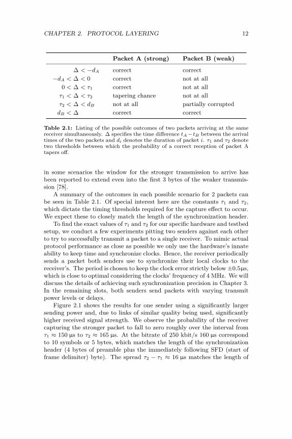
0 < ∆ < τ1 correct not at allτ1 < ∆ < τ2 tapering chance not at allτ2 < ∆ < dB not at all partially corrupteddB < ∆ correct correct

Table 2.1: Listing of the possible outcomes of two packets arriving at the samereceiver simultaneously. ∆ specifies the time difference tA− tB between the arrivaltimes of the two packets and di denotes the duration of packet i. τ1 and τ2 denotetwo thresholds between which the probability of a correct reception of packet Atapers off.

in some scenarios the window for the stronger transmission to arrive hasbeen reported to extend even into the first 3 bytes of the weaker transmis-sion [78].

A summary of the outcomes in each possible scenario for 2 packets canbe seen in Table 2.1. Of special interest here are the constants τ1 and τ2,which dictate the timing thresholds required for the capture effect to occur.We expect these to closely match the length of the synchronization header.

To find the exact values of τ1 and τ2 for our specific hardware and testbedsetup, we conduct a few experiments pitting two senders against each otherto try to successfully transmit a packet to a single receiver. To mimic actualprotocol performance as close as possible we only use the hardware’s innateability to keep time and synchronize clocks. Hence, the receiver periodicallysends a packet both senders use to synchronize their local clocks to thereceiver’s. The period is chosen to keep the clock error strictly below ±0.5µs,which is close to optimal considering the clocks’ frequency of 4 MHz. We willdiscuss the details of achieving such synchronization precision in Chapter 3.In the remaining slots, both senders send packets with varying transmitpower levels or delays.

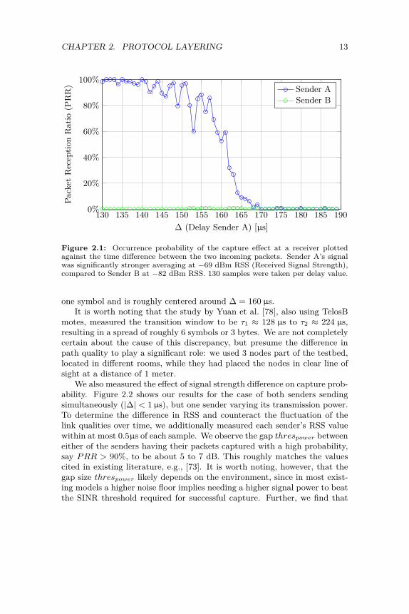
Figure 2.1 shows the results for one sender using a significantly largersending power and, due to links of similar quality being used, significantlyhigher received signal strength. We observe the probability of the receivercapturing the stronger packet to fall to zero roughly over the interval fromτ1 ≈ 150 µs to τ2 ≈ 165 µs. At the bitrate of 250 kbit/s 160 µs correspondto 10 symbols or 5 bytes, which matches the length of the synchronizationheader (4 bytes of preamble plus the immediately following SFD (start offrame delimiter) byte). The spread τ2 − τ1 ≈ 16 µs matches the length of


130 135 140 145 150 155 160 165 170 175 180 185 1900%

20%

40%

60%

80%

100%

∆ (Delay Sender A) [µs]

Pack

etR

ecep

tion

Rat

io(P

RR

) Sender ASender B

Figure 2.1: Occurrence probability of the capture effect at a receiver plottedagainst the time difference between the two incoming packets. Sender A’s signalwas significantly stronger averaging at −69 dBm RSS (Received Signal Strength),compared to Sender B at −82 dBm RSS. 130 samples were taken per delay value.

one symbol and is roughly centered around ∆ = 160 µs.It is worth noting that the study by Yuan et al. [78], also using TelosB

motes, measured the transition window to be τ1 ≈ 128 µs to τ2 ≈ 224 µs,resulting in a spread of roughly 6 symbols or 3 bytes. We are not completelycertain about the cause of this discrepancy, but presume the difference inpath quality to play a significant role: we used 3 nodes part of the testbed,located in different rooms, while they had placed the nodes in clear line ofsight at a distance of 1 meter.

We also measured the effect of signal strength difference on capture prob-ability. Figure 2.2 shows our results for the case of both senders sendingsimultaneously (|∆| < 1 µs), but one sender varying its transmission power.To determine the difference in RSS and counteract the fluctuation of thelink qualities over time, we additionally measured each sender’s RSS valuewithin at most 0.5µs of each sample. We observe the gap threspower betweeneither of the senders having their packets captured with a high probability,say PRR > 90%, to be about 5 to 7 dB. This roughly matches the valuescited in existing literature, e.g., [73]. It is worth noting, however, that thegap size threspower likely depends on the environment, since in most exist-ing models a higher noise floor implies needing a higher signal power to beatthe SINR threshold required for successful capture. Further, we find that


−12 −10 −8 −6 −4 −2 0 +2 +4 +6 +80%

20%

40%

60%

80%

100%

(RSSA −RSSB) [dB]

Pack

etR

ecep

tion

Rat

io(P

RR

)

Sender ASender B

Figure 2.2: Occurrence probability of the capture effect at a receiver plottedagainst the power difference between the two incoming packets. Sender A’s trans-mit power was varied over its whole available range, producing RSSA values from−89 dBm to −68 dBm, while Sender B’s transmit power was kept constant, pro-ducing RSSB values from −79 dBm to −76 dBm. 40 samples were taken for eachof the available 32 transmit power values, resulting in a total of 1108 compara-ble instances, i.e., instances in which we were able to measure both senders’ RSSvalues.

the probability of either packet to be received successfully drops to around5% when the signal strengths are identical.

In conclusion, we observe that in order to be able to reliably call onthe capture effect in a slotted setup (see next section), competing sendersshould have a clock difference below 160 µs and a power difference above5 dB. This level of synchronization we can achieve by synchronizing aboutonce every few minutes.

2.4 Layering Protocols

2.4.1 Slot LogicTraditionally, executing multiple protocols in parallel is likely to incur apenalty on the utilization of the network resources and/or the performanceof the protocols themselves. For example, if two protocols access the mediumalternatingly using time slots, up to half the slots may be wasted, while oneof the protocols is idle and the other has demand for more than its share


of time slots. Further, in this scenario, information propagation latency isdoubled, as no information can leave a node sooner than 2 slots after its ar-rival. Using more opportunistic approaches, such as when using CSMA/CA(Carrier Sensing Multiple Access with Collision Avoidance), the problemsmentioned above do not occur: any number of idle protocols do not influ-ence the network’s utilization or the performance of the other protocols.However, when the load on the network becomes too large, unfairness andstarvation become threats to effective operation.

In this section, we will detail our proposed method of parallelizing, or lay-ering, k protocols with the aim of combining the benefits of the approachesmentioned above: no unused network resources under load, while also of-fering fairness and prevention of starvation. Further, our method allowsprioritization of protocols, giving higher-priority protocols almost completeaccess to the network’s resources at the cost of possible starvation of lower-priority protocols in areas of the network not sufficiently separated fromthe high-priority traffic in space or time. Finally, this section will discusshow network topology and environment influence the number of layers ourmethod can support.

The core idea is to deliberately provoke the capture effect at every nodewhenever it is destined to receive multiple packets at the same time. Todo so, we enforce time slotting and require the clock difference betweenany two nodes within a node’s immediate neighborhood to be below τ1 (seeSection 2.3). By ensuring all potentially competing packets start within atime interval of length τ1, we obtain that which packet is to be received ina time slot is solely dependent on the arriving packets’ signal strengths, butnot on their relative timings. Given a sufficient spread in signal strengths,the capture effect is almost certain to enable successful reception of thepacket with the strongest signal. We will discuss why this assumption is areasonable one to make below.

The next piece of the scheme is to use transmission power control at eachsender to specify the “layer” of each packet. As nodes may have varyingdistances and link qualities to each other, the transmission power cannotsimply be derived from the layer of the packet to be sent, but must considerthe destination node. In effect, for every receiving node a set of incomingsignal strength intervals needs to be chosen, different enough to be distin-guishable by the capture effect, but similar enough to fit within the rangeof signal strengths each of the neighboring nodes can produce. Thus, forevery sending node, for each of its neighbors and for each of the layers thecorrect sending power needs to be determined.

Finally, every protocol is uniquely assigned to a layer. We label thelayers 1, . . . , k, where the protocol of layer k has the highest priority andthe protocol of layer 1 has the lowest. Every slot, every node executes


Algorithm 1: Pseudocode for Slot Logicout← ∅foreach protocol Pl with layer l ∈ {1, . . . , k} do

Pl.compute slot()if Pl.outgoing packet 6= ∅ then

out← Pl.outgoing packetPl.outgoing packet ← ∅

if out 6= ∅ thenTransmit out this slot (using the correct power for out’s targetand layer).

elseListen this slot.in← incoming packetif in 6= ∅ then

Pin.layer.process packet(in)

Algorithm 1: First, it performs each protocol’s slot computation separately,while storing the packet the highest layer protocol wants to send (out) anddiscarding all others. If any packet was chosen this way, it is sent at thesending power corresponding to its destination and protocol layer. If nopacket was chosen, the node listens for the duration of that slot and deliversany received packet to the correct protocol.

This setup attempts to give each protocol the illusion of being the onlyprotocol present. This is achieved by protocols experiencing a “packet loss”if a protocol of higher layer is active at the same time: if a higher layer isoverriding the sending of a lower layer packet, that lower layer packet simplyappears to have been lost in transit; conversely, if a packet of a higher layer isoverriding the reception of a lower layer packet, that packet’s fate appearsindistinguishable from true packet loss as well. As occasional packet lossis a common occurrence in almost every environment due to noise burstsor interference, most wireless algorithms are innately capable of recoveringfrom a loss of packets. Hence, they are perfectly suitable to be used as lowerlayer protocols. The highest layer protocol experiences no packet loss dueto the presence of other layers (with one exception noted below), but is stillsubject to the usual environmental impediments. If the environment is infact controlled enough to not suffer any such packet loss, as might be thecase in clinical settings such as perhaps data centers, a protocol relying ona low packet loss ratio may be used as the highest layer.

We do not consider queuing packets from multiple protocols desiring tosend from the same node in the same slot, as this would tamper with pos-


sible protocol-internal slot schedules of protocols whose packets have beendelayed. This would damage the illusion, and require significant changesto the way protocols for use in the lower layers are designed, such thatcommon known protocols can no longer easily be used. Simulating packetloss is hence a cleaner solution, while the option of allowing layering-awareprotocols to immediately know if their packet was dropped, such that theymay queue it for the next slot if desired, is still available.

There is one scenario, however, in which the illusion inevitably breaksdown. As we are assuming that the wireless hardware is not capable ofreceiving while transmitting, a problem occurs when a node is choosing tosend in a slot due to a protocol of layer i, but would in the same slot receive apacket on layer j > i. Here the protocol of layer j will experience packet lossdue to a lower layer protocol. Unfortunately, it is impossible to prevent thisscenario from occurring without also introducing significant overhead to allother scenarios: if the traffic demand on layer j can occur spontaneously, forinstance, to propagate an alarm event, every node’s layer i protocol may bein any state, including having chosen to send in that particular slot. If oneforces layer i a priori to not send in certain slots, the latency and bandwidthpenalties tied to TDMA are inevitable.

We found that for applications, in which the highest level protocol aimsto achieve the lowest latency possible (such as the example application dis-cussed in Section 2.5), a reasonable workaround is to send every high-prioritypacket twice in successive time slots. Note that while this does double theamount of packets sent, the latency only increases when the described sce-nario indeed occurs. Running common algorithms, a node that is sendingin slot t is unlikely to send again in slot t+ 1 as there would not have beenany input in slot t to instigate another outgoing transmission. This is eventrue if multiple layers wanted to send in slot t, as all their packets wouldhave been either sent or discarded in slot t. Hence, a high-priority packetsent in two successive time slots is bound to arrive in at least one of the twoslots.

2.4.2 Power ChoicesThe main difficulty now lies in ensuring a good spread in the signal strengthsof all packets received at each node in the same slot. One assumption wemake is that the individual protocols avoid causing multiple of its packetsto collide at the same node. This is reasonable especially for protocolsfollowing the traditional school of thought, which dictates all simultaneouspacket arrivals to be fatal collisions. Given this assumption and the fact thatevery protocol runs on its own unique layer, all packets arriving at a nodein the same slot belong to different layers and should thus have sufficiently


different signal strengths for the capture effect to be able to enable receptionof the strongest packet.

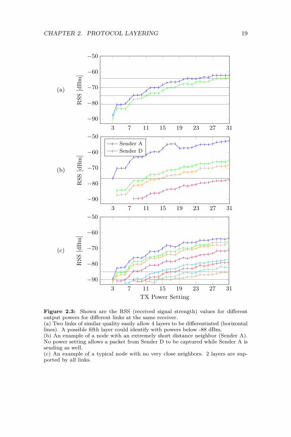
There exists a tradeoff between the number of available layers (and thusnumber of parallelizable protocols) and the achievable spread of received sig-nal strengths at each node. The network topology and in particular the ho-mogeneity of the network’s link qualities play a large role in enabling a highernumber of layers to be well separated at each node. “Well-separatedness”requires the difference in received signal strength between every pair of lay-ers to exceed the threshold of threspower (which we found to be at least 5 dBon our testbed, see Section 2.3). We found that in a perfectly homogeneoussetting where every link is either of high quality (high range of powers us-able for successful transmissions) or not of significant power, the number ofavailable layers becomes maximal. Using our hardware we found up to 4 or5 sending powers to be distinguishable at a receiver, see Figure 2.3(a). Sucha high number of layers (4 or more) is likely only feasible in settings with ahigh degree of control over node positioning and environmental influences.

More commonly, networks contain varying levels of heterogeneity, withsome areas containing only long-distance/low-quality links, some areas moretightly packed with low-distance/high-quality links, and many areas be-ing cases in between. For our hardware, especially these in-between casesspell trouble due to the granularity of selectable sending powers decreas-ing sharply as power values decrease, see Figure 2.4. As a direct result, abottleneck for the number of layers forms at nodes with both long-distanceand short-distance links. In the example of Figure 2.3(b), the low-qualitylink of Sender D can only provide receive powers in the range from -89 to-78 dBm, a range which Sender A cannot reach with any power setting.In Figure 2.3(c), while no extremely high-quality links are included, thehigher-quality links still offer only a very low power granularity in the rangefeasible for lower-quality links.

We find that for our hardware 2 clearly distinguishable layers are possiblein essentially all topologies, but identify the occurrence of both “long” and“short” links at a single node as the main bottleneck. Note that the causefor the bottleneck is not present in nodes which have only long or only shortlinks, as in these cases the links’ power ranges overlap very well. Essentially,the smaller the upper bound on the difference between the longest andshortest link at any node in the network, the higher the number of availablelayers.

When faced with the problem of the network supporting too few well-separated layers, there are several possible solutions. For one, the problemmay be addressed directly by excluding or repositioning such mixed-linknodes or some of their neighbors. Another alternative is to employ wire-less transceivers offering better-suited transmission power control options.


3 7 11 15 19 23 27 31

−50

−60

−70

−80

−90

(a)R

SS[d

Bm

]

3 7 11 15 19 23 27 31

−50

−60

−70

−80

−90

(b)

RSS

[dB

m]

Sender ASender D

3 7 11 15 19 23 27 31

−50

−60

−70

−80

−90

(c)

TX Power Setting

RSS

[dB

m]

Figure 2.3: Shown are the RSS (received signal strength) values for differentoutput powers for different links at the same receiver.(a) Two links of similar quality easily allow 4 layers to be differentiated (horizontallines). A possible fifth layer could identify with powers below -88 dBm.(b) An example of a node with an extremely short distance neighbor (Sender A).No power setting allows a packet from Sender D to be captured while Sender A issending as well.(c) An example of a typical node with no very close neighbors. 2 layers are sup-ported by all links.


3 7 11 15 19 23 27 31−30

−20

−10

0

TX Power Setting

Out

put

Pow

er[d

Bm

]

Figure 2.4: The 32 available output power settings on the CC2420 wirelesstransceiver [75]. Note that half the available values cover only a 7 dB intervaland settings below 3 are not usable.

Finally, in some scenarios compromising the quality of the layer separationa bit by lowering the required signal strength spread at each receiver maybe feasible, especially if only few or unimportant nodes are affected. Lat-ter may lead to occasional inadvertent inversion of packet priorities andtrue destructive packet collisions, which some applications may be able totolerate.

If one wishes to have multiple protocols to have the same priority and beentitled to equal share of the medium, it is not advisable to assign both pro-tocols the same layer of receive powers. Since packets of the same strengtharriving at a node will not trigger the capture effect but instead lead to de-structive packet collisions, none of the packets would be decoded correctly.Instead, we recommend having a separate layer for each protocol, but rotat-ing through the protocol assignments for the layers on a slot number basis.I.e., for two protocols, simply swap their layer assignments every c slots.We suggest choosing the value of c to be around 50 to 100 to avoid eachprotocol suffering very frequent packet loss when both protocols are underload.


8

33

3

6

16

22

28

18 27 24

23

3231

10

Figure 2.5: A part of the FlockLab testbed which we used to conduct our ex-periments on. An example of a convergecast tree with node 8 as the root node isshown. Yellow edges indicate links not part of the tree. To avoid collisions withinthe convergecast layer, no two sibling branches connected by links may executesimultaneously. Hence, every node, once it is woken, first queries all its black edgechildren in parallel, and then, in a second step, its blue edge children.

2.5 Example Application

To verify and measure the effectiveness of our method on real world wirelesssensor networks, we chose an example application highlighting the supposedbenefits of our method and implemented it on FlockLab [46] which spansthe floor of an office building (see Figure 2.5).

We consider the scenario of fire detectors covering the rooms of a buildingwith the goal of reporting the outbreak of a fire as quickly as possible to abase station, or root node, which to the network is just a normal node with aspecial role. The root node has a wired connection to the building facilitiesand can escalate the alarm if it is informed of a fire by one of its neighbors.In its wireless capability it matches a regular node and as such it can onlyhear a local neighborhood of nodes, necessitating the propagation of a firealarm over multiple hops.

Additionally, we require the liveness and proper functioning of all nodesto be regularly verified so that defunct nodes may be replaced in a timelymanner. We regard these liveness tests to be of less urgency than the firealarms and thus do not mind fire alarms having priority access to the wireless


medium. Hence, in our model the liveness tests will be executed as a protocolon layer 1, while the fire alarm propagation will take place as a protocol onlayer 2.

We model each fire detector as a TelosB sensor node extended with asmoke sensor, though for this experiment we only simulate a virtual smokesensor to make alarm generation easier. The TelosB sensor node features aCC2420 wireless transceiver [75], which supports the IEEE 802.15.4 wire-less standard [32] and is capable of either sending or receiving on a singlefrequency at a time. It uses a synchronization header for detecting the startof packets and offers output power control, but does not provide any moreadvanced features such as message in message or decoding more than onetransmission at a time. For all intents and purposes it fulfills the ideal ofa “standard” low-power wireless interface as was referred to in Sections 2.3and 2.4.

2.5.1 Layer 1We design the layer 1 protocol as a parallelized convergecast on a tree over-laid onto the network connectivity graph. Every node knows of its parentand its children in the tree as well as the adjacency relationships between itschild branches. The root node repeatedly initiates convergecasts and will,whenever a node is indicated as missing or defunct by the output of the con-vergecast, generate an appropriate alert for that node’s replacement. Thislayer will also resynchronize a node’s clock whenever it receives a messagefrom its parent in the tree. This ensures the packet transmission synchro-nization requirements for achieving the capture effect hold over the time ofthe deployment.

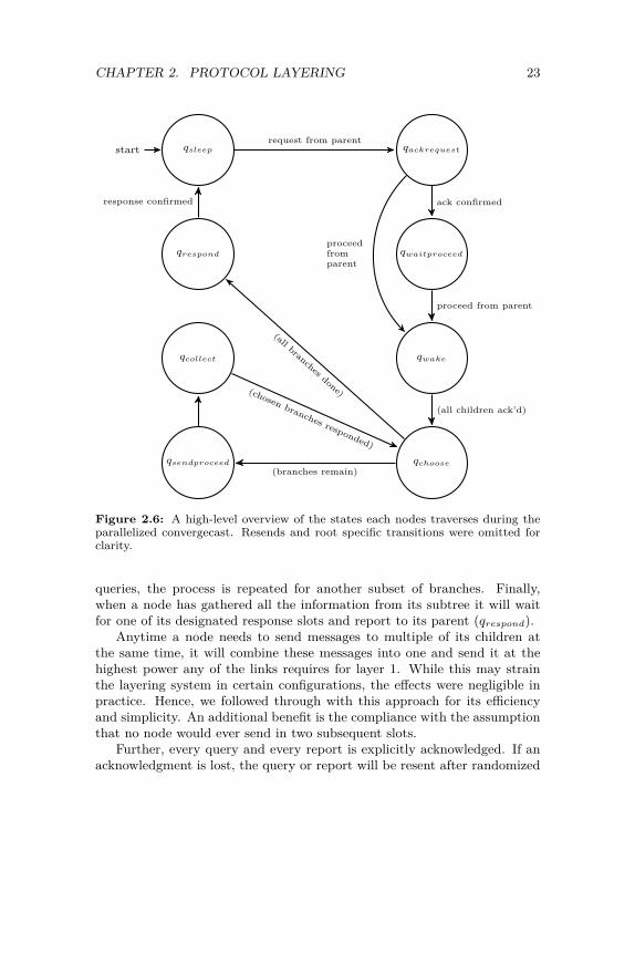
The states each node goes through as it participates in the convergecastare depicted in Figure 2.6. The root node begins a convergecast by wakingup itself and skipping to qwake (since it has no parent). Other nodes startin qsleep and wait for a request from their parent. After acknowledging therequest (qackrequest) their parent will send some of its children proceed mes-sages (qwake), while the remaining children only receive acknowledgmentsand will have to wait at first (qwaitproceed). After “proceeding” a node wakesits children with a request of its own and then proceeds to qchoose.

Once a node has woken all its children it will start querying subsets of itschildren (qsendproceed), such that the branches of no two chosen children areadjacent in the same subset. With every proceed message, every addressedchild is assigned a recurring slot during which it may confirm the query(not pictured) and then later send a response, once it has gathered all theinformation from its branch. Once a subset of branches has completed,by each branch either sending a report or not responding for 3 subsequent


qsleepstart qackrequest

qwaitproceed

qwake

qchoose

qrespond

qsendproceed

qcollect

request from parent

ack confirmed

proceedfromparent

proceed from parent

(all children ack’d)

(all branches done)

(branches remain)

response confirmed

(chosen branches responded)

Figure 2.6: A high-level overview of the states each nodes traverses during theparallelized convergecast. Resends and root specific transitions were omitted forclarity.

queries, the process is repeated for another subset of branches. Finally,when a node has gathered all the information from its subtree it will waitfor one of its designated response slots and report to its parent (qrespond).

Anytime a node needs to send messages to multiple of its children atthe same time, it will combine these messages into one and send it at thehighest power any of the links requires for layer 1. While this may strainthe layering system in certain configurations, the effects were negligible inpractice. Hence, we followed through with this approach for its efficiencyand simplicity. An additional benefit is the compliance with the assumptionthat no node would ever send in two subsequent slots.

Further, every query and every report is explicitly acknowledged. If anacknowledgment is lost, the query or report will be resent after randomized


exponentially growing backoff intervals until an acknowledgment is receivedor, in the case of a query, the recipient is pronounced dead after 3 attempts.Once a node is determined to be dead, it will be ignored for the remainderof the convergecast and the root node, upon receiving the aggregated nodedata, can notify building personnel to manually check on the potentiallybroken node. If a node retrying reports is queried for a new convergecast,it will snap out of its clearly erroneous state and participate as per usual inthe new convergecast.

2.5.2 Layer 2The fire alarm propagation is implemented on layer 2, i.e., a layer with ahigher priority than the convergecasts described above. When an alarmevent occurs it is propagated along a tree towards the root, a tree similar oreven identical to the one used by layer 1. We simulate smoke alarm eventsoccurring randomly and independently with a chance of 1% each slot. In afirst test series, we trigger the event at one random node only (SA). In aseparate test series we trigger multiple alarm events (MA) at different nodessimultaneously or with a few slots delay as might happen in the case of theoutbreak of a real fire.

Multiple simultaneous alarms introduce an additional difficulty to thelayer 2 protocol. As mentioned in Section 2.4.1, even the protocol withhighest priority needs to deal with packet loss due to addressed nodes possi-bly not listening as they might be sending out a packet of their own on layer1. The solution mentioned previously, to repeat all packets of the highestlayer once in the subsequent slot, is not sufficient here due to the possiblepresence of multiple alarms, which in our setting all need to have the samepriority (as we only have 2 layers available) and are hence expected to pos-sibly collide destructively. Thus, we additionally implemented implicit andexplicit acknowledgments for alarm propagation. When a node receives analarm packet from a descendant in the tree, it forwards it in both of thenext two slots and then listens. If it hears an ancestor in the tree propagatethe alarm, it takes this as an implicit acknowledgment and calms down, i.e.,no longer spreads the alarm. If it does not hear the alarm propagated, itrepeats it another two times after a random exponentially growing backoffperiod, and listens again. A node which hears the same alarm again (afterit had already propagated it) does not propagate it again. If the sender wasa direct descendant, it sends back an explicit acknowledgment.

We also considered solving the collision of multiple alarms by tracking thereceived signal strength indicator (RSSI) when no packet is being receivedin a slot. We expected to see a signal strength similar to or stronger thanthat of a layer 2 packet, which would indicate that an alarm had occurred


for certain, even if the exact data of the alarm was unavailable. This wouldallow us to pass on the existence of an alarm without incurring a latencypenalty from the alarm collision. Unfortunately, experiments showed theRSSI to not be reliable enough of a measure for the presence of layer 2packets, producing an unacceptably high rate of either false positives orfalse negatives.

2.5.3 DiscoveryTo determine the trees to be used by layers 1 and 2 as well as the differentreception power levels for each layer at each node, we initially perform a“discovery” phase. The goal of this phase is to record the quality of eachlink in the network, compute the trees with the smallest possible heightand then inform each node of its parent, its children and all the parametersrequired for operation as listed above.

While in our experiments we needed to perform this phase only a singletime, in practice it would likely be desirable to repeat this phase every sooften to deal with changes in the wireless environment, as, for instance,may easily be caused by the closing of doors or the increasing of a room’sair temperature or humidity. Such repeated runs may for the most part beexecuted solely on layer 1 without impacting the operationally critical alarmpropagation on layer 2, the potential exception being tests of links at highersending powers. In our experience, some links’ qualities can drasticallychange every few seconds, while others are stable for days. Reasonably, onewould not perform a complete discovery as often as every few seconds orminutes, but rather on the order of hours while testing known fluctuatinglinks more frequently.

2.6 Test Results

We compare the performance of our method to a traditional approach, whichdoes not incorporate the capture effect but for comparability’s sake adheresto the time slotting. It will, however, still execute both of the protocols (con-vergecast and alarm propagation) and is aware of their relative priorities.Hence, it will prefer forwarding alarm packets over sending convergecastrelated packets, but will use the same transmission power for all packets.Additionally, we compare the latency of the alarms as well as the dura-tions of the convergecasts to the best physically possible values. Since thesevalues usually are not obtainable without a dose of luck with regards to low-reliability long-range links, we do not expect these values to consistently bemet.


Alarms Convergecasts

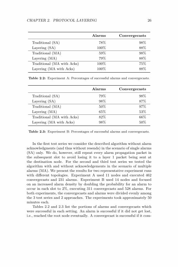
Traditional (SA) 78% 98%Layering (SA) 100% 88%Traditional (MA) 59% 98%Layering (MA) 79% 88%Traditional (MA with Acks) 100% 75%Layering (MA with Acks) 100% 88%

Table 2.2: Experiment A: Percentages of successful alarms and convergecasts.

Alarms Convergecasts

Traditional (SA) 79% 98%Layering (SA) 98% 87%Traditional (MA) 50% 97%Layering (MA) 65% 53%Traditional (MA with Acks) 82% 66%Layering (MA with Acks) 98% 50%

Table 2.3: Experiment B: Percentages of successful alarms and convergecasts.

In the first test series we consider the described algorithm without alarmacknowledgments (and thus without resends) in the scenario of single alarms(SA) only. We do, however, still repeat every alarm propagation packet inthe subsequent slot to avoid losing it to a layer 1 packet being sent atthe destination node. For the second and third test series we tested thealgorithm with and without acknowledgements in the scenario of multiplealarms (MA). We present the results for two representative experiment runswith different topologies. Experiment A used 11 nodes and executed 462convergecasts and 231 alarms. Experiment B used 14 nodes and focusedon an increased alarm density by doubling the probability for an alarm tooccur in each slot to 2%, executing 311 convergecasts and 528 alarms. Forboth experiments, the convergecasts and alarms were divided evenly amongthe 3 test series and 2 approaches. The experiments took approximately 50minutes each.

Tables 2.2 and 2.3 list the portions of alarms and convergecasts whichwere successful in each setting. An alarm is successful if it did not get lost,i.e., reached the root node eventually. A convergecast is successful if it com-


pleted correctly and collected data from every single node. The tendencyof the layered approach to promote alarms over convergecasts even morethan the traditional approach is clearly visible: while our layering approachgenerally suffers from fewer successful convergecasts, it beats the successfulalarm ratio of the traditional approach, reaching an almost certain alarmdelivery. The difficulty of dealing with multiple alarms without acknowl-edgements is also apparent, as alarms inevitably get lost. Of special note isthe fact that while the traditional approach reaches the same 100% alarmsuccesses as us using acknowledgements in experiment A, it suffers a largerconvergecast success penalty.

Figures 2.7 and 2.8 show the CDF (cumulative distribution function)for the alarm delay. The delay of an alarm is defined as the number ofslots it takes to reach the root node minus the physical minimum numberof slots required to traverse the multi-hop path from its origin to the root.This allows for a comparison between alarms originating at different nodes.We observe our approach beating the traditional one in each category, notleast because it suffers fewer lost alarms, with the exception of “MA withacknowledgements” in experiment A. For single alarms we achieve an alarmdelay of 2 slots or less in 85% resp. 94% of cases, which is excellent consider-ing the optimal reference alarm delay taking unreliable long-distance linksinto account. As was to be expected, overall the maximum delay experi-enced without acknowledgements is around 4 slots, while acknowledgementsallows alarm reporting to be drawn out considerably.

Figures 2.9 and 2.10 shows a similar CDF for convergecast delays, de-fined as a convergecast’s duration minus the minimum amount of slots ouralgorithm requires for the convergecast even if not a single packet was lost.The considerably worse performance of our approach here is due to it caus-ing the layer 1 algorithm increased packet loss in order to support layer 2.Also of note is the general increase in delay for both approaches as morelayer 2 traffic is introduced, both by adding acknowledgements and resendsand by increasing the amount of alarms.

2.7 Summary and Future Work

We presented a method to execute multiple protocols in parallel, givingeach protocol the illusion of being the only one and having complete accessto the network’s resources. When a higher-priority protocol uses networkresources, such as the ability of a node to send or receive a packet in a spe-cific slot, lower-priority protocols experience this as packet loss, as sendingpriority or the capture effect drop lower-priority packets.

Further, in theory our method causes no overhead in terms of time slot


0 5 10 150%

20%

40%

60%

80%

100%

Alarm Delay [slots]

CD

F

Traditional (SA)Layering (SA)Traditional (MA)Layering (MA)Traditional (MA with Acks)Layering (MA with Acks)

Figure 2.7: Experiment A: Distributions of alarm delay.

0 5 10 150%

20%

40%

60%

80%

100%

Alarm Delay [slots]

CD

F

Figure 2.8: Experiment B: Distributions of alarm delay.


0 5 10 15 20 250%

20%

40%

60%

80%

100%

Convergecast Delay [slots]

CD

F

Traditional (SA)Layering (SA)Traditional (MA)Layering (MA)Traditional (MA with Acks)Layering (MA with Acks)

Figure 2.9: Experiment A: Distributions of convergecast delay.

0 5 10 15 20 250%

20%

40%

60%

80%

100%

Convergecast Delay [slots]

CD

F

Figure 2.10: Experiment B: Distributions of convergecast delay.


use and latency. To confirm this, we implemented an example applica-tion with 2 protocols of different priorities and measured their performance.The results show very few packet losses and essentially optimal latency forthe higher-priority protocol, while it causes additional losses to the lower-priority protocol compared to a traditional approach. In the scenario thatboth approaches can avoid loss of high-priority packets, our method does sowhile incurring less overhead to the lower-priority protocol.

Our technique does come with some downsides, most notably the removalof the individual protocols’ ability to employ some options directly relatedto the physical layer. These options include power control, knowledge aboutcorrupted packets, the use of the capture effect and the ability to not usetime slotting. For many algorithms these features may be non-critical oreven completely irrelevant. For others it may make this technique unsuitableor require significant changes. Further, the connectivity graph is likely tolose some edges on one or more layers whose target reception power rangescannot be met by the respective senders’ transmission power ranges. Thisespecially affects the availability of long-range links on the lower-prioritylayers.

Our technique proves to be flexible concerning hardware and existingprotocols, allowing it to be deployed without much additional overhead be-yond implementing the discovery phase and basic slot logic. We have shownsimple low-power hardware such as TelosB to be sufficient and pointed outhow our technique is capable of masking the existence of competing pro-tocols, allowing many protocols to simply be “dropped in” on one of thelayers, possibly even on-the-fly. Some protocols may greatly benefit frombeing aware of the other protocols, for instance, by knowing when theirpacket was dropped already at the sender, or by even directly communi-cating with the higher layer protocols on the same node. We believe thiswork to nevertheless be a useful first step in the direction of exploring suchmulti-layer protocols.

Incidentally, our technique is also a feasible fairness provider in manysituations. While in its basic implementation it will in fact allow any pro-tocol to completely starve all protocols with a lower priority, as discussedin Section 2.4.2, by periodically reassigning the layers to different protocols,each protocol can be assigned an arbitrary share of the network resourceswhen averaged over longer periods of time. However, our approach is likelynot suitable for applications with a need for temporally more fine-grainedQoS. This is under the assumption that under load each protocol is able towork more efficiently if it is the top active layer for its critical region forlonger consecutive time intervals than for many smaller ones, separated byspurs of time with possibly 100% packet loss.

Power consumption was not examined as part of our tests. We believe

this issue to be almost orthogonal to the problems discussed here, as dutycycling and rate of packets sent are not affected by the proposed method.If nodes are unable to maintain synchronization through a sleep phase, careneeds to be taken that they are resynchronized before attempting to send apacket intended to evoke the capture effect. On TelosB hardware, however,staying below the synchronization error threshold of 160µs for longer periodsof time is very easy due to its 32 kHz crystal oscillator (with a tick length ofabout 31 µs) being able to power-efficiently and accurately keep time evenwhen the CPU is in sleep mode. While operation on higher-priority layersdoes require larger transmission powers, for many applications the proposedmethod may remain a desirable choice, especially if high-priority messagesare more of an exception than a rule (as in our fire alarm example).

Promising future work includes applying this method to wireless hard-ware with a finer power control granularity, especially at the low power end.We expect such hardware to make it significantly easier to support a largernumber of layers while still having a clear separation of layers. In general, itis also worth investigating the capture effect parameters for a layering setupon other hardware, as hardware more amenable to exhibiting the captureeffect may loosen the requirements on synchronization or layer separation.

If the lack of absolute network resource control for higher layers provesto be an issue (i.e., if lower layers are preventing reception of high layerpackets by sending lower layer packets), various solutions may be worthexploring. For example, one could depart a little from strict slotting andhave higher layers send their packets a few dozen symbol durations earlier,as to allow prevention of lower layer sending. Alternatively, a mechanismby which higher layers completely reserve some nodes for a period of timeis imaginable and may be very effective depending on the application.

3Maintaining Constructive Interference

3.1 Introduction

In recent years, the benefits of constructive interference (CI) have beendiscovered for wireless sensor networks: By synchronizing identical signalswell enough, the interference caused by the collision is not destructive butrather unnoticeable or even strengthening. On the one hand, this allowsthe development of algorithms which can expect identical packets not todestructively interfere. On the other hand, more unstable and longer linkscan be used more reliably through the strengthening of the signal.

Traditionally, the frugal nature of sensor node hardware and timekeepingmoved synchronizing clocks and transmissions out of reach for commoditysensor nodes. In the past, several workarounds have been proposed to nev-ertheless enable the signals of separate nodes to interact meaningfully:

• One way is to provide a highly accurate external global clock sourceby some means, e.g., GPS, with each sensor node.

• Another approach is to forgo the ability to send fully articulated datapackets – and to simply transmit waveforms instead, which are unlikelyto fatally destructively interfere [20].

33

• Most recently, Glossy [19] explored how to leverage incoming referencepackets to send a packet immediately afterwards with an almost con-stant delay. When multiple nodes use the same reference packet (ordifferent well-synchronized reference packets), their outgoing packetsare then synchronized enough to achieve CI.

All of these approaches have in common that they try to avoid dealingwith the rather unreliable internal clocks of commodity sensor nodes. Inthis chapter, we explore the possibilities of creating synchrony sufficient forharnessing CI without relying on any of these workarounds. By meticulouslykeeping time using the available local clocks to extrapolate a global timevalue, and by minimizing the variance in packet departure delay, we manageto at least partially obtain this goal. In particular, we present a proof ofconcept implementation achieving CI on the popular TelosB sensor nodes,confirming the viability of our approach: Even for only 2 senders we obtainan increase in signal strength of at least 2 dB in 60% of cases and an increasein packet reception ratio of 20–35% when signal strengths are equal. Forideal results, we need the last synchronization of the senders to lie at most 20seconds in the past when attempting to send simultaneously, but even aftermultiple minutes of sleep our approach can benefit from CI. We carefullycompare several parameters in order to understand the limits of CI on sensornodes. For instance, already a synchronization error in the order of 1 µs isproblematic. More precisely, as we are using the IEEE 802.15.4 standard,the transmissions need to start within less than 0.5µs of each other to avoiddestructive interference.

Hence, a significant part of this chapter is dedicated to synchronizing theclocks of the sensor nodes, maintaining this synchrony and, finally, preciselydictating the time span of the wireless transmission. Clock synchronizationfor wireless nodes in general is a well-studied problem, but the synchroniza-tion precision requirements by our setup are more stringent than those ofthe common use cases such as TDMA.

3.2 Related Work

3.2.1 Clock SynchronizationTime synchronization between network nodes has been studied for a longtime even before wireless nodes became widespread. The 30 years old Net-work Time Protocol (NTP) [55] is still in use today for time synchroniza-tion between two machines over the Internet, achieving accuracies of about10 ms. Recently, adjustments have been proposed improving its accuracyto about 1 millisecond [43], which is still off by a factor of over 1000 from

the precision we require.Wireless networks face additional challenges [16] but also have addi-

tional options at their disposal due to the different nature of their medium.Romer [67] proposes a synchronization algorithm focusing on sparse adhoc networks. Dozer [3] minimizes energy consumption by keeping sender-recipient pairs synchronized over long periods of time and only rarely wakingthem for brief scheduled rendezvous exchanges. To maintain synchrony inspite of clock drift, the drift is modeled and compensated for. We employ asimilar scheme, see Section 3.5.3.

RBS [15] makes use of the broadcasting nature of every wireless transmis-sion to synchronize multiple nodes with a single transmission. RBS achievessynchronization accuracy on the order of microseconds. TPSN [21] builds ahierarchical tree structure for synchronization from a root node. TPSN alsointroduces the concept of MAC layer timestamping, which we build upon inthis work (see Section 3.5.2). FTSP [53, 54] floods periodical synchroniza-tion waves through the network, improving accuracy to around 1µs. Furtherimprovements for synchronizing networks of nodes are RITS [68], reactivelysynchronizing nodes using global events, and RATS [37] and PulseSync [41],which propose rapid network-wide flooding while employing schedules toavoid collisions.

An analysis of the single-hop and multi-hop performance of the differentsynchronization protocols and a proposal for a non-hierarchical synchroniza-tion method improving the multi-hop case can be found in [31].

3.2.2 Constructive InterferenceAlready early on, primarily flooding algorithms became privy to the possiblegains of using non-interfering signals and thus being able to flood the net-work without the overhead of building and adhering to a flooding schedule.We distinguish single and multiple source flooding: while in single sourceflooding a node desires to disseminate information or an event in the wholenetwork, in multiple source flooding any number of nodes may raise redun-dant alarm events which need to be propagated. Lu et al. [49] proposed thesingle source flooding protocol Flash, which relies on the capture effect toresolve collisions between neighboring nodes at the flooding front.

Slotos [20] implemented multiple source flooding in form of an alarm sys-tem in which an alarm signal, a simple waveform, was propagated througha network by nodes which received the alarm starting to send out the signalas well. In this case the concurrent signals were not artificially aligned butthe resulting amount of destructive interference was acceptable to the pro-tocol, as the signal did not carry any data beyond its existence. Similarly,Black Burst Synchronization (BBS) [23] employs non-destructively interfer-

ing pulses, so called “black bursts”. Dutta et al. [13] discovered that auto-matic acknowledgments of multiple nodes having received the same packetwill in fact be synchronized so well as to cause constructive interference. Au-tomatic acknowledgments are a common wireless transceiver feature that al-lows an immediate response to correctly received packets (as verified by thepacket’s checksum). As the acknowledgment is completely handled by thehardware, this feature avoids any variable desynchronizing delays the mi-croprocessor software may cause. While essentially all of these approacheshave the common disadvantage of having very little control over the databeing sent, this is well suited for multiple source flooding, as such eventstypically are not expected to carry detailed information.

More recently, Ferrari et al. [19] took the idea of synchronizing to theend of a previously received packet one step further and proposed Glossy:instead of sending an acknowledgment, which does not allow for the trans-mission of meaningful data, they prepare a full response packet during thereception of the incoming packet. By immediately issuing its transmissionwhen the transceiver indicates the completion of the reception of the in-coming packet, the variable delays microprocessor software code paths andclock skew can introduce are minimized. As the packet contents sent bythe different responders still have to be the same to allow constructive in-terference, flooding is the main application for this approach as well. Theconstructive interference leads to improved signal strengths, making weakerand longer links more viable. Further, the rapid forwarding leads to excep-tionally short flooding durations. Several recent protocols are based on therapid data dissemination capability of Glossy [11,18,38,79] and various stud-ies on its reliability and the conditions necessary for creating constructiveinterference have been conducted [78,80].

To achieve CI, Glossy relies on tying the departure time of each packetto the end of the incoming transmission of a previous packet. One of themain goals of this chapter is to do away with this restriction, yet still attainCI for data packets rather than be restricted to mere events.

3.3 Experiment Setup

3.3.1 HardwareThe TelosB sensor node [62] we use for our experiments is mainly comprisedof a 16-bit RISC microcontroller, the TI MSP430, and a TI CC2420 wirelesstransceiver. The clocks available to the MSP430 are a 32 kHz (215 Hz) quartzcrystal as well as an internal digitally controlled oscillator (DCO) whichserves as the pulse generator for the instruction execution. The frequency ofthe DCO is very prone to being skewed through fluctuations in temperature

and voltage, but can generally be configured to be anywhere in the rangefrom 100 kHz to 5 MHz.

The CC2420 is tailored to support IEEE 802.15.4 and offers many con-venience features such as framing given packet data including automaticallyincluding a 16-bit CRC checksum field in the packet footer. We rely on thischecksum mechanism as our main way to tell whether a received packet hasbeen corrupted. The CC2420 offers a range of transmit powers from -30dBm to 0 dBm (see Figure 2.4). We make use of this feature as it is easierto adjust the output power than to physically move the nodes every timechanges in the environmental conditions require it (see Section 3.7).

We made use of an installation of 30 of these sensor nodes part of Flock-Lab, placed at various locations on a floor of an office building near theceiling, some inside enclosed offices, some on the hallway. This allowed usto consider a variety of real life scenarios.

3.3.2 SoftwareOn the sensor nodes we run code based on Contiki [12] version 2.7. Wechose Contiki because it allows making the kind of low-level modificationswe required the easiest. In particular, we overhauled the clock module whichis concerned with using the MSP430’s Timer A (configured with the 32 kHzquartz crystal as clock source) to count elapsed seconds and periodically testfor expired user-defined timers. We decrease the time span between timerinterrupts to 2−10 seconds, and instead of counting elapsed seconds we countthe occurrences of overflow interrupts for the Timer A timer register.

Contiki also offers a mechanism to periodically re-configure the DCO tobest match the desired frequency. We make use of this to keep the DCOfrequency near 222 Hz (roughly 4 MHz), the highest supported power-of-twomultiple of the quartz crystal frequency (215 Hz). This essentially subdivideseach tick of the quartz crystal into 27 sub-ticks, i.e., increasing the combinedprecision by 7 bit (see Section 3.5.1).

The DCO is usually turned off to conserve energy during idle low-powerphases of the processor. While our approach allows such sleep phases, wenaturally do require the DCO to have been running since at least the lastquartz crystal tick to be able to provide accurate timestamps. This incursan overhead of up to 2−15 seconds of DCO operation after each wake-up.

We also configure the CC2420 driver to not use CCA (clear channel as-sessment) for packet transmission and extend it to support recording 64-bittimestamps on incoming packets and adding 64-bit timestamps to outgoingpackets (see Section 3.5.2).

For the process of the experiments themselves see Section 3.7.1.

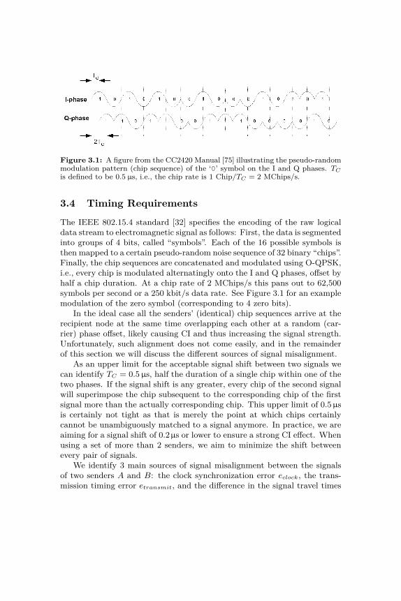
Figure 3.1: A figure from the CC2420 Manual [75] illustrating the pseudo-randommodulation pattern (chip sequence) of the ‘0’ symbol on the I and Q phases. TC

is defined to be 0.5 µs, i.e., the chip rate is 1 Chip/TC = 2 MChips/s.

3.4 Timing Requirements

The IEEE 802.15.4 standard [32] specifies the encoding of the raw logicaldata stream to electromagnetic signal as follows: First, the data is segmentedinto groups of 4 bits, called “symbols”. Each of the 16 possible symbols isthen mapped to a certain pseudo-random noise sequence of 32 binary “chips”.Finally, the chip sequences are concatenated and modulated using O-QPSK,i.e., every chip is modulated alternatingly onto the I and Q phases, offset byhalf a chip duration. At a chip rate of 2 MChips/s this pans out to 62,500symbols per second or a 250 kbit/s data rate. See Figure 3.1 for an examplemodulation of the zero symbol (corresponding to 4 zero bits).

In the ideal case all the senders’ (identical) chip sequences arrive at therecipient node at the same time overlapping each other at a random (car-rier) phase offset, likely causing CI and thus increasing the signal strength.Unfortunately, such alignment does not come easily, and in the remainderof this section we will discuss the different sources of signal misalignment.

As an upper limit for the acceptable signal shift between two signals wecan identify TC = 0.5µs, half the duration of a single chip within one of thetwo phases. If the signal shift is any greater, every chip of the second signalwill superimpose the chip subsequent to the corresponding chip of the firstsignal more than the actually corresponding chip. This upper limit of 0.5µsis certainly not tight as that is merely the point at which chips certainlycannot be unambiguously matched to a signal anymore. In practice, we areaiming for a signal shift of 0.2µs or lower to ensure a strong CI effect. Whenusing a set of more than 2 senders, we aim to minimize the shift betweenevery pair of signals.

We identify 3 main sources of signal misalignment between the signalsof two senders A and B: the clock synchronization error eclock, the trans-mission timing error etransmit, and the difference in the signal travel times

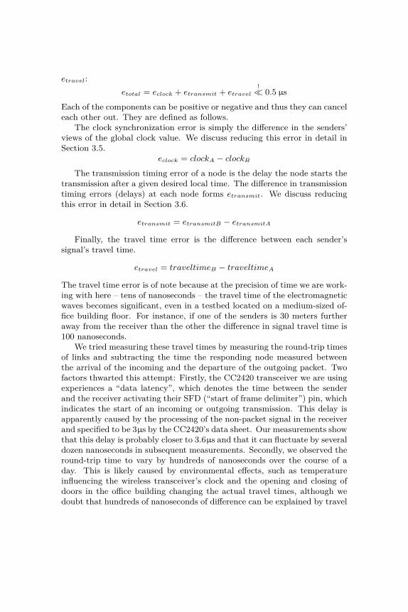
etravel:etotal = eclock + etransmit + etravel

!� 0.5 µs

Each of the components can be positive or negative and thus they can canceleach other out. They are defined as follows.

The clock synchronization error is simply the difference in the senders’views of the global clock value. We discuss reducing this error in detail inSection 3.5.

eclock = clockA − clockB

The transmission timing error of a node is the delay the node starts thetransmission after a given desired local time. The difference in transmissiontiming errors (delays) at each node forms etransmit. We discuss reducingthis error in detail in Section 3.6.

etransmit = etransmitB − etransmitA

Finally, the travel time error is the difference between each sender’ssignal’s travel time.

etravel = traveltimeB − traveltimeA

The travel time error is of note because at the precision of time we are work-ing with here – tens of nanoseconds – the travel time of the electromagneticwaves becomes significant, even in a testbed located on a medium-sized of-fice building floor. For instance, if one of the senders is 30 meters furtheraway from the receiver than the other the difference in signal travel time is100 nanoseconds.

We tried measuring these travel times by measuring the round-trip timesof links and subtracting the time the responding node measured betweenthe arrival of the incoming and the departure of the outgoing packet. Twofactors thwarted this attempt: Firstly, the CC2420 transceiver we are usingexperiences a “data latency”, which denotes the time between the senderand the receiver activating their SFD (“start of frame delimiter”) pin, whichindicates the start of an incoming or outgoing transmission. This delay isapparently caused by the processing of the non-packet signal in the receiverand specified to be 3µs by the CC2420’s data sheet. Our measurements showthat this delay is probably closer to 3.6µs and that it can fluctuate by severaldozen nanoseconds in subsequent measurements. Secondly, we observed theround-trip time to vary by hundreds of nanoseconds over the course of aday. This is likely caused by environmental effects, such as temperatureinfluencing the wireless transceiver’s clock and the opening and closing ofdoors in the office building changing the actual travel times, although wedoubt that hundreds of nanoseconds of difference can be explained by travel

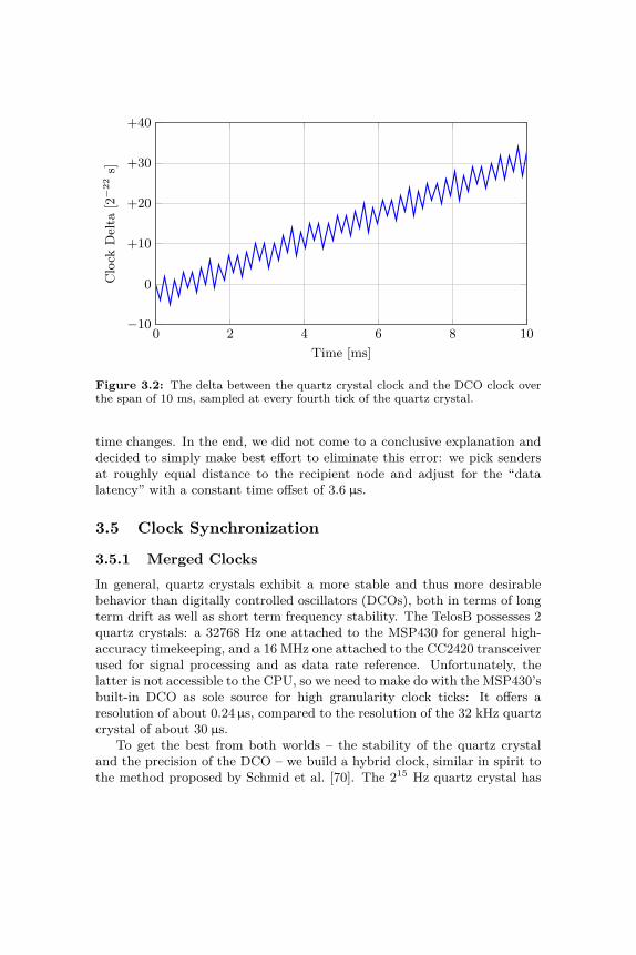
0 2 4 6 8 10−10

0

+10

+20

+30

+40

Time [ms]

Clo

ckD

elta

[2−

22s]

Figure 3.2: The delta between the quartz crystal clock and the DCO clock overthe span of 10 ms, sampled at every fourth tick of the quartz crystal.

time changes. In the end, we did not come to a conclusive explanation anddecided to simply make best effort to eliminate this error: we pick sendersat roughly equal distance to the recipient node and adjust for the “datalatency” with a constant time offset of 3.6 µs.

3.5 Clock Synchronization

3.5.1 Merged ClocksIn general, quartz crystals exhibit a more stable and thus more desirablebehavior than digitally controlled oscillators (DCOs), both in terms of longterm drift as well as short term frequency stability. The TelosB possesses 2quartz crystals: a 32768 Hz one attached to the MSP430 for general high-accuracy timekeeping, and a 16 MHz one attached to the CC2420 transceiverused for signal processing and as data rate reference. Unfortunately, thelatter is not accessible to the CPU, so we need to make do with the MSP430’sbuilt-in DCO as sole source for high granularity clock ticks: It offers aresolution of about 0.24µs, compared to the resolution of the 32 kHz quartzcrystal of about 30 µs.

To get the best from both worlds – the stability of the quartz crystaland the precision of the DCO – we build a hybrid clock, similar in spirit tothe method proposed by Schmid et al. [70]. The 215 Hz quartz crystal has

Figure 3.3: The final layout of our timestamps with the different clock sources indifferent rows. The quartz clock has priority over the DCO clock, so actually only7 bits of the DCO clock are used. No clock we use is able to specify the lowest 8bits, but these bits allow for storing extra precision when a timestamp is the resultof arithmetic operations.

priority and ensures relatively high stability over the long term while theDCO, set to a speed as close to 222 Hz as possible, fills out the time spanin between the quartz crystal ticks with 222/215 = 27 finer-grained ticks.To accomplish this, we configured the MSP430 to copy the current value ofthe DCO clock (a 16-bit counter) at each quartz crystal tick into a specialcapture register. The MSP430 allows doing this in parallel with regularinstruction execution at no additional overhead. A complete current timevalue could then be obtained by subtracting the current DCO counter fromthe value in the special capture register and using the result as 7 bits ofadditional precision together with the current quartz crystal counter. Addi-tionally, we keep the number of times the quartz crystal counter overflowedin a variable. This variable is incremented in an overflow interrupt handlercausing a negligible overhead every 2 seconds. Figure 3.2 shows how a sep-arate DCO clock would move in relation to the quartz crystal. Not only isthere a clear drift and oscillating behavior (both of which could be accountedfor to some degree), but there also is a notable amount of randomness thatwould make relying on the DCO alone as a clock source a poor choice.

As all the MSP430’s registers only hold 16 bits, the question of the sizefor timestamps arises, as for the transmission between nodes they should beunambiguous, at least within a period of several seconds. 16-bit variablesdo not suffice as the DCO clock alone wraps around 256 times a second.32-bit variables would only wrap every 1024 seconds or roughly 17 minutes,but since we want to enhance our timestamps by an additional 8 bits ofprecision when extrapolating (see Section 3.5.3), we settled on 64-bit vari-ables. Such variables are well supported by our compiler (a GCC variant

for the MSP430), but special care has to be taken when performing arith-metic operations on variables of this size, as they quickly grow to requirehundreds of instructions on 16-bit RISC CPUs such as the MSP430. Thefinal layout of our timestamps can be seen in Figure 3.3. The precision ofthese timestamps is 2−30 seconds, roughly a nanosecond, and the range issufficiently large (several years).

3.5.2 MAC Layer TimestampingTo synchronize the sending nodes’ clocks, a reference node sends a coupleof synchronization packets at the start of each round (see Section 3.7.1). Totransmit synchronization information we employ MAC layer timestamping[21]. This technique generally involves capturing the local time at the startof an arriving or departing packet using an specialized output pin of thewireless transceiver (the aforementioned “SFD pin”) connected to a timercapture input pin of the CPU. The sender writes the captured timestamp tothe footer of the outgoing packet while the transmission of the of the packetis ongoing. The receiver in turn can then compare its captured timestampto the timestamp contained in the footer to obtain an accurate local timevalue for the shared event of the start of the packet.

Contiki’s CC2420 driver already provides this feature, but only supports16-bit timestamps from the 32 kHz quartz crystal. We extend the driverto support our mixed-source 64-bit timestamps. As mentioned above, as-sembling such a 64-bit timestamp from its individual components requiresa fair amount of instructions on this architecture – a total of 55 in our case.Further, we also already apply drift compensation at this stage, which re-quires the multiplication of two 64-bit integer variables, which result in anadditional few hundred instructions. As our synchronization packets are 60bytes in length, which require roughly 2 ms or 8500 CPU cycles to transmit,there is still ample time to compute this timestamp and insert it at the endof the packet.

3.5.3 Drift CompensationAlthough the properties of quartz crystals are generally rock-solid, their fre-quencies are not completely set in stone: temperature changes affect theirfrequency and multiple instances of the same crystal may have slightly differ-ent frequencies. In a system with multiple such quartz crystals this leads toobservable clock drift: clocks which were synchronized at some point in timemay drift apart as a result of their ever so slightly varying speeds. Worse,these speeds change over time as the environment temperature changes.

To combat this, we implemented a drift compensation mechanism basedon linear regression with a rolling buffer: For the last k received synchro-nization packets we store (locali, offseti) pairs, where locali is the localtime at which the ith synchronization packet was received and offseti =globali − locali was the clock offset at that time. We then compute on thelast k values:

drift = locali · offseti − locali · offseti

local2i − locali2

baseoffset = offseti − drift · locali

where exp denotes the average of the expression exp for i ∈ {n, n − 1, n −2, . . . , n − k + 1} and n denotes the number of received synchronizationpackets. To extrapolate an estimate of the global time we compute:

globalest(local) = local + baseoffset + drift · local.

For the size of the rolling buffer we found k = 8 to be adequate, adaptingto changes quickly enough, while avoiding wild fluctuations from noise andoutliers. Other settings with less frequent synchronization rounds mightfind smaller values to suit their needs better.

While drift compensation is absolutely crucial in situations where nodesare not re-synchronized for longer periods of time, it can already offer sub-stantial benefits after shorter periods when high precision is required. To beable to store and forward global timestamps computed using the formulasabove while preserving the gained precision, we append 8 additional bits toour timestamps (see Figure 3.3).

Figure 3.4 shows the quality of the clock synchronization that we wereable to achieve using both MAC layer timestamping and drift compensa-tion. We observe most instances (over 70%) to be spread uniformly be-tween −250 and +250 nanoseconds. We cannot hope to improve this bymuch since our clocks are only granular to 2−22 seconds. Hence, each clockreading introduces an error distributed uniformly at random in the interval[−2−23 seconds,+2−23 seconds] (roughly [−120 ns,+120 ns]).

Figure 3.5 shows the development of the synchronization error betweentwo nodes which were synchronized a couple of times at the start (to allowfor drift detection) and then not anymore. Clearly, not employing driftcompensation when not re-synchronizing nodes over longer periods of timeis fatal to the synchronization error. The almost constant slope shows whylinear regression is the right tool to combat clock drift. We also see inthis example that, in spite of drift compensation, the synchronization errorexceeds 0.5µs after about 25 seconds. Hence, when attempting simultaneoussending, the most recent synchronization should ideally not lie further than10 or 20 seconds in the past.

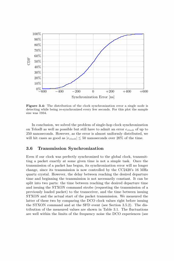
−600 −400 −200 0 +200 +400 +6000%10%20%30%40%50%60%70%80%90%

100%

Synchronization Error [ns]

CD

F

Figure 3.4: The distribution of the clock synchronization error a single node isdetecting while being re-synchronized every few seconds. For this plot the samplesize was 1934.

In conclusion, we solved the problem of single-hop clock synchronizationon TelosB as well as possible but still have to admit an error eclock of up to250 nanoseconds. However, as the error is almost uniformly distributed, wewill hit cases as good as |eclock| ≤ 50 nanoseconds over 20% of the time.

3.6 Transmission Synchronization

Even if our clock was perfectly synchronized to the global clock, transmit-ting a packet exactly at some given time is not a simple task. Once thetransmission of a packet has begun, its synchronization error will no longerchange, since its transmission is now controlled by the CC2420’s 16 MHzquartz crystal. However, the delay between reaching the desired departuretime and beginning the transmission is not necessarily constant. It can besplit into two parts: the time between reaching the desired departure timeand issuing the STXON command strobe (requesting the transmission of apreviously loaded packet) to the transceiver, and the time between issuingSTXON and the actual start of the packet transmission. We measured thelatter of these two by comparing the DCO clock values right before issuingthe STXON command and at the SFD event (see Section 3.5.2). The dis-tribution of the measured values are shown in Table 3.1. The fluctuationsare well within the limits of the frequency noise the DCO experiences (see

0 120 240 360 480 600 720 840 960

0

+1

+2

+3

+4

+5

Time [s]

Sync

hron

izat

ion

Erro

r[m

s] Without Drift CompensationWith Drift Compensation

0 30 60 90 120 150−8

−6

−4

−2

0

Time [s]

Sync

hron

izat

ion

Erro

r[µ

s]

Figure 3.5: Synchronization error of a single node over time.

tSFD − tSTXON Instance Count Fraction of Total

1593 15 0.26%1594 893 15.71%1595 3726 65.53%1596 1049 18.45%1597 3 0.05%

Σ 5686 100.00%

Table 3.1: Measured STXON→SFD times collected from a single test run with15 nodes. The time differences are specified in DCO ticks.

Figure 3.2). While it is possible that there is a small variable delay, it is notdiscernible and we assume this time span to be constant.

It remains to scrutinize the time span between reaching the target timeand issuing STXON. Initially, we employed busy waiting: once the targettime was close, we stop relinquishing control to the operating system andenter a loop in which all we do is query the time until the target timehas been passed. Immediately after, we call the driver routine to start thetransmission (one of the first instructions of which is to issue STXON).

Listing 3.1: Simple Busy Waitif (TargetTime - GetGlobalTime() < 10 ms) {

while (TargetTime > GetGlobalTime()); // do nothing

cc2420_driver.transmit();}

This approach experiences a large variance in loop exit times and thustransmission times (relative to the target time) due to the large amountof instructions within the loop: assembling the local timestamp requires55 instructions, computing the global time from it requires at least 110 in-structions and comparing it to the target time requires 22 instructions. Toaddress this problem we made 3 changes. The first change was to applyour model of the global time “backwards” to compute the target local timebefore entering the busy wait loop. The second change was to decomposethe target local time into its 3 clock sources (see Figure 3.3) and spin onthe 3 16-bit clocks one after another. These two changes reduce each loopto the minimum of 4 instructions. See Listing 3.2 for an approximate im-plementation. TAR is the quartz counter register, TBR is the DCO counterregister and TBCCR6 contains the value of TBR at the last quartz crystaltick.

Listing 3.2: Busy Wait Split by Clock Sourcesvoid await(uint64_t local_target) {

uint16_t target_tarof = (local_target >> 23) & 0xFFFF;

while (TAR_overflows < target_tarof);

uint16_t target_tar = (local_target >> 7) & 0xFFFF;while ((TAR - target_tar) & 0x8000)

;

uint16_t target_tbr = (local_target & 0x007F) + TBCCR6;while ((TBR - target_tbr) & 0x8000)

;}

It is worth noting that not every instruction requires the same amount oftime to be executed. However, due to the absence of caches and pipeliningin the MSP430’s architecture, the execution time of any given instructioncan be specified exactly in terms of a number of CPU cycles, which directlycorrespond to the impulses generated by the DCO.

Listing 3.3: Busy Wait Assembly.L36:

mov &__TBR, r15 ; 3 cyclessub r12, r15 ; 1 cyclecmp #0, r15 ; 2 cyclesjl .L36 ; 2 cycles

The third and final change we made was to insert NOPs (1-cycle “nooperation” instructions) ahead of the final loop to ensure we exactly matchedthe target time when exiting the final loop. The four instructions comprisingthe loop execute in exactly 8 cycles (see Listing 3.3), so before the loop wewait for (target tbr - TBR) mod 8 cycles by using a jump table into aseries of NOPs. We note that we could save 2 cycles by merging the cmpand jl instructions into a single jn instruction (2 cycles), an optimizationwhich our compiler did not apply. However, such a change would affect theachieved synchronization only in extremely rare cases.

After applying these optimizations, the time offset between the targettime and the issuing of the STXON command strobe was constant in over80% of cases. By artificially delaying the next periodic timer interrupt beforeentering the last busy-wait loop to a point 1 ms in the future, this numberincreased to > 99% of cases.

The constant delay is easily adjusted for, leaving the only remainingtransmission error we can observe the delay between issuing STXON andregistering the SFD event as measured by the DCO clock. Note that in thiscase the DCO clock is used only for measuring and does not in any way

influence the wireless transceiver preparing for the transmission. Thus, it isa reasonable assumption that the jitter seen in Table 3.1 is merely a productof the DCO’s instability, albeit we cannot rule out that the transceiver itselfintroduces a small variable delay.

Finally, as with clock synchronization, we suffer a transmission erroretransmit of up to 250 nanoseconds, the resolution of our most precise clock,independent of the clock synchronization error. However, this error is alsodistributed uniformly in the interval [−2−23 seconds,+2−23 seconds] and ina certain fraction of all samples |etransmit| will be acceptably small.

3.7 Constructive Interference

3.7.1 Experiment ProcedureA particular concern when designing the experiments was to ensure we wouldbe able to discern which transmissions were successful due to CI and whichwere successful due to the capture effect. For the capture effect to occur,the “captured” transmission needs to be slightly stronger than the sum ofthe remaining transmissions’ signal powers. On our testbed we found therequired extra signal power to vary between 2 or 3 dB, highly depending onthe nodes (see Figure 3.6). As link qualities in real life scenarios and on ourtestbed can easily vary by ±3 dB within minutes or sometimes even mereseconds, completely avoiding power settings in which the capture effect canoccur is not feasible. To nevertheless be able to detect the capture effect,we thus frequently measure the quality of every link used. For a detailedexplanation of the capture effect refer to Section 2.3.

In our experiments we considered several tuples of nodes, where one nodeof each tuple was designated the receiver and was known to have somewhatstable links to the other nodes, the senders. We proceed in rounds, in whichfirst we let all senders send simultaneously twice: first with the same datapacket and then with data packets individual to the senders. Then, as asecond stage, each of the senders sends alone once. Finally, the receiver givesthe senders feedback on the round and optionally also supplies them withfresh synchronization information. During each round the senders keep theirsending powers constant. The purpose of the second stage is to ensure weknow the received signal strengths (RSS) for all senders. Because a roundtakes less than half a second, we make the assumption that the wirelessenvironment does not change significantly during the vast majority of allrounds. Knowing the difference in RSS values is vital for us, as it allows usto discern successful receptions which may have been caused by the captureeffect, as discussed above. We fix one of the senders’ transmission powersat a medium value, such that the other senders will be able to create RSS

values both stronger and weaker than the fixed sender. These other sendersiterate over a range of power settings whose limits are regularly adaptedbased on the feedback received between rounds.

3.7.2 ResultsFirst, consider the case of 2 senders. Figure 3.6 shows the relation betweenthe difference in received signal strengths (RSS) and the packet receptionratio (PRR) for senders sending the same data versus sending different data,in which case the senders would set every symbol of the packet payload to asymbol corresponding to their ID. A large positive RSS difference meanssender B, which is iterating over different transmission powers over therounds, was received a lot stronger than sender A, whose transmission powerstays constant. Which sender was received can be seen when different datais sent, as is shown by the dashed lines. These plots are particularly in-teresting because they highlight the interplay of CI and the capture effect:if either sender is received a lot more strongly than the other, it will bereceived correctly regardless of it sending a different packet. However, asthe signal powers become more similar, destructive interference occurs moreoften. By sending the same data, we are able to avoid a portion of thedestructive interference, strongly implying the occurrence of CI.

We were able to observe CI to varying degrees for any triplet of nodes, aslong as the senders are capable of creating signals with similar strength at thereceiver. As a result of CI the PRR observed at equal RSS increases by 25–35% of samples. The width of the gap between one sender dominating andthe other sender dominating appears to be a property of the hardware andenvironment of a certain node tuple, but does not appear to be connectedto the CI we achieve.

Figure 3.7 displays the distribution of the signal strength gained throughCI at equal RSS for 2 senders. We observe a large variation both due to aninherent gray area in link quality and due to the variation in transmissionsynchrony achieved. However, in over 65% of cases we measure an increaseof signal strength by 2 dB or more.

We also conducted experiments with 3 and 4 senders, making an evenlarger case for CI as the capture effect is known to occur less and less asthe number of senders increases [49]. Tables 3.2, 3.3 and 3.4 display thePRRs aggregated in two different ways for one run with 3 senders and onerun with 4 senders. Empty cells correspond to configurations with fewerthan 5 samples. While there is a significant fluctuation in values due to theunavoidably low number of samples in many cells, as we cannot dictate theRSS values, a few clear trends can be observed. Most visibly, the same datacase usually exhibits a PRR 25–40% higher than the different data case.

−6 −5 −4 −3 −2 −1 0 +1 +2 +3 +4 +5 +60%

20%

40%

60%

80%

100%

(a)

PRR

−6 −5 −4 −3 −2 −1 0 +1 +2 +3 +4 +5 +60%

20%

40%

60%

80%

100%

(b)

PRR

−6 −5 −4 −3 −2 −1 0 +1 +2 +3 +4 +5 +60%

20%

40%

60%

80%

100%

(c)

RSSB −RSSA [dB]

PRR

Same Data Different Data (Either Sender)Different Data (Sender A) Different Data (Sender B)

Figure 3.6: The PRR plotted against difference in RSS for two senders for 3different node triplets, clearly showing CI occurring at a RSS difference close tozero for each triplet, while the capture effect causes larger differences to almostalways succeed. (a) and (b) show two pairs of senders with differing behavior. (c)depicts the result of deliberately mistiming one of the senders by 1 µs, preventingany CI from occurring.

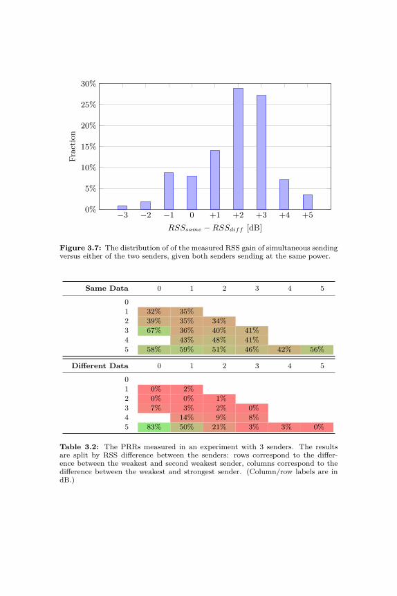
−3 −2 −1 0 +1 +2 +3 +4 +50%

5%

10%

15%

20%

25%

30%

RSSsame −RSSdiff [dB]

Frac

tion

Figure 3.7: The distribution of of the measured RSS gain of simultaneous sendingversus either of the two senders, given both senders sending at the same power.

Same Data 0 1 2 3 4 5

01 32% 35%2 39% 35% 34%3 67% 36% 40% 41%4 43% 48% 41%5 58% 59% 51% 46% 42% 56%

Different Data 0 1 2 3 4 5

01 0% 2%2 0% 0% 1%3 7% 3% 2% 0%4 14% 9% 8%5 83% 50% 21% 3% 3% 0%

Table 3.2: The PRRs measured in an experiment with 3 senders. The resultsare split by RSS difference between the senders: rows correspond to the differ-ence between the weakest and second weakest sender, columns correspond to thedifference between the weakest and strongest sender. (Column/row labels are indB.)

Same Data 0 2 6 10

0 34%2 36% 38% 56%4 51% 48% 52% 50%6 70% 91% 78% 62%8 100%

Different Data 0 2 6 10

0 2%2 1% 2% 0%4 23% 10% 12% 0%6 80% 78% 50% 24%8 67%

Table 3.3: The same data as in Table 3.2, aggregated differently: the results aresplit by average RSS difference to the strongest sender (rows) and the varianceamongst the powers of the non-strongest senders (columns). (Column/row labelsare in dB.)

Same Data 0 2 4 6 8 10

0 10%2 23% 24% 36% 21% 17%4 30% 32% 30% 18% 9% 56%6 25% 34% 36% 33% 22%8 50% 50% 50%

Different Data 0 2 4 6 8 10

0 0%2 1% 0% 0% 0% 0%4 1% 1% 2% 0% 0% 0%6 4% 6% 9% 6% 6%8 30% 28% 29%

Table 3.4: The same aggregation as in Table 3.3, but for a different experimentwith 4 senders.

Further, the capture effect, whose occurrence can easily be discerned fromthe different data case, occurs more often the further the strongest sender’ssignal strength is from the rest (bottom left in Table 3.2, bottom and toa lesser degree also left in Tables 3.3 and 3.4). Finally, particularly highvalues can be found in the bottom right of Table 3.2, which are likely aresult of the possibility of the two much stronger signals invoking both CIas well as the capture effect to survive the occasional timing errors in theweakest signal.

As a further confirmation of our approach, we also conducted a few runsof the experiment in which we configured one of the senders to deliberatelysend 1µs late. The expectation is to have this completely remove all possibil-ity for CI. The result of one such run can be seen in Figure 3.6(c), exhibitingalmost no CI at all. This underlines the importance of the synchronizationprecision we strove for. Similarly, when increasing the resynchronization in-terval we found the effect to diminish after varying periods of time: in somecases as soon as after 30 seconds, in others not for multiple minutes. Thiscan be attributed to the clock synchronization error rising due to changesin clock drift which drift compensation can no longer account for (see Fig-ure 3.5).

For the packets sent by the senders we used payload sizes ranging from 12to 26 bytes. Together with the 2 final checksum bytes, 4 bytes of preambleand 1 SFD byte, transmissions were thus 19−−33 bytes or 608−−1056 µsin length. The different packet sizes did not exhibit a significant differencein performance.


We determined a bound for the total allowable error for CI to occur, andconsidered three the error sources of clock synchronization error, transmis-sion synchronization error and travel time error:

etotal = eclock + etransmit + etravel

!� 0.5 µs

We reduced eclock by combining the TelosB’s 32 kHz quartz crystal withthe MSP430’s DCO to obtain a stable 4 MHz clock, and we reduced etransmit

by optimizing our transmission code path down to the CPU cycle. Both ofthese values were minimized into the range of the length of a single clocktick (2−22 s). In an attempt to reduce etravel, we picked senders such thatthey had roughly the same distance to the receivers.

Using our example implementation we conducted several experimentswith 2 to 4 senders trying to create CI by simultaneously sending the samepacket to a recipient node. To ensure packets were not arriving merely due

to the capture effect we also sent packets with differing data. Our resultsshow an increase in signal strength of at least 2 dB in 60% of cases for2 senders, and an increase in PRR of 20–35% for any amount of senderswhen signal strengths are equal. Considering we expected to only meetthe necessary signal alignment requirements in the fraction of samples, inwhich both eclock and etransmit happened to be small enough, these 20–35%appear quite satisfactory and are likely mainly held back by the precisionof the underlying hardware.

While our implementation and results are based on the TelosB and the802.15.4 standard, we believe the concepts to apply in a similar fashion tomost sensor nodes and wireless standards. Further, there are two propertiesthe TelosB was lacking, which were stunting our results: 1) a clock with aprecision a magnitude higher than the used chip length and 2) a transceiverdesigned for a similar precision in transmission timing.

In conclusion, we showed that maintaining the option of CI on commod-ity sensor node hardware over longer periods of time is feasible, throughextraordinary inter-node synchronization and without incurring the over-head of a global “wave” of synchronizing packets before every transmissionrequiring CI.

4Capturing Attention Using theCapture Effect

4.1 Introduction

Wireless networks have been around for a long time, and almost alwaysthe participating nodes adhere to a simple setup: There is a sender whichtransmits data to a single receiver or a set of receivers. More recently, thissetup increasingly includes multiple antennas on both sides (multiple-inputand multiple-output, MIMO). However, conceptually, we still have a singlesender trying to transmit a packet to a (set of) receiver(s).

In this chapter, we introduce a third party, a “third man” in the formof a second sender. This second sender tries to capture the attention of thereceiver(s) using the capture effect. The second sender ignores the standardrules of wireless communication, and blatantly transmits during the trans-mission of the first sender. The second transmitter could transmit duringthe payload of the original packet, or during its header. We want the sec-ond sender to be stronger than the first sender, either by being closer to thereceiver(s), or by transmitting with more power.

We present two scenarios benefiting from such unorthodox behavior.However, we believe that the general idea of having a second sender may

55

have potential beyond our two examples.Our first scenario addresses networks with partially low density, e.g.,

where a few nodes failed and the network was separated into two or moreparts that can hardly communicate with each other. Consider the case of aspread out multi-hop wireless network containing a “chasm”, i.e., a virtualor physical gap between two parts of the network across which links arevery poor, as illustrated in Figures 4.1 and 4.2. Even if the network stillforms a connected graph via routes around the chasm using only stable links,these detours incur a large latency and medium usage overhead due to theadditional hops packets have to make.

By sending across the chasm we might collect several partially incorrectlyreceived packets at multiple nodes on the receiving side. These erroneouscopies may then be pieced together to obtain a completely correct copy of thesent packet. However, if already the synchronization header is not receivedcorrectly at a node, that node will not recognize the incoming packet andhence will not be able to record it. By employing a node broadcasting afake synchronization header on the receiving side, we are able to ensure thatevery node which is a candidate for receiving at least parts of the packet islistening. This improves the chances of correctly receiving every part of thepacket in some cases from less than 5% to about 30%.

The second scenario we discuss makes use of what we call the packet-in-packet communication primitive: Here, the second sender does not transmitduring the header, but during the payload of the first sender’s packet. Assuch, the second sender may inject a short packet into concurrently ongoingtransmissions using the capture effect. Doing so, the time and control mes-sage overhead for avoiding collision between high-priority and low-prioritytraffic can be reduced to a minimum. This is particularly beneficial whenthe high-priority traffic consists of short spontaneous bursts.

Naively sending a high-priority packet into an ongoing transmission witha sufficient power differential for the capture effect to occur (about 4–5 dBon TelosB) results in the inserted packet being decoded correctly in onlyabout 5% of cases. However, with proper improvements, we can bring thisvalue up to 70%.

In particular, we apply two techniques to improve the success rates inboth scenarios: 1) improving transmission synchronization and 2) repairingmisinterpreted symbols where possible.

1) By improving transmission synchronization we increase the chanceof the symbols of the strong/injected and the weak/base packet to overlayclosely enough, such that the symbols have a high chance of being decodedproperly. In the chasm scenario this results in a complete packet transmis-sion in 25% of cases. For packet-in-packet this improves the correct decodingrate to about 40%.

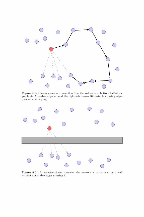
Figure 4.1: Chasm scenario: connection from the red node to bottom half of thegraph via A) stable edges around the right side versus B) unstable crossing edges(dashed and in gray).

Figure 4.2: Alternative chasm scenario: the network is partitioned by a wallwithout any stable edges crossing it.

2) Among the remaining bad cases we observe many to experience adeterministic mapping of values on the injected symbols. By reversing thismapping we are able to repair some of the bad cases, raising the total correctdecoding rate to 30% in the chasm scenario and to 70% in the packet-in-packet scenario.

We implement proofs of concept of these techniques based on Contikifor both scenarios on TelosB and test them on the FlockLab testbed.

4.2 Related Work

The inherent multi-hop topology of wireless sensor networks as well as theunique properties of the wireless medium have enabled the inception ofseveral new communication primitives. In particular, most recently, waysto induce constructive interference through concurrent forwarding of a singletransmission have been explored [18,19]. Constructive interference can boostsignal quality and allows rapid network flooding without the overhead of acarefully planned flooding schedule. Another example is the deliberate useof the capture effect, which was previously thought of as a nuisance. Yet itis now counted on more and more to resolve collisions without experiencingdestructive interference, which most classical models would predict [76] (seealso Chapter 2).

Much like the previous two chapters, our work in this chapter also mainlyfalls into this field of medium access primitives. However, one of our scenar-ios also deals with the topic of unreliable links. To avoid repeating ourselvestoo much, we will omit some of the related work here and refer the gentlereader to Sections 2.2 and 3.2.

The popular Glossy protocol [19] provides a technique by which sim-ple single antenna sensor nodes could send with unprecedented synchrony,leading to a fast single source flooding algorithm avoiding collisions throughconstructive interference and the capture effect. This technique is based ontying the departure time of each packet to the end of the incoming transmis-sion of the previous packet, effectively reducing the timespan during whichclock skew can erode synchrony. For the scenarios examined in this chapter,a Glossy-like mechanism is not applicable, as 1) the presence of a commonreference packet for all senders is not guaranteed and in fact impossible inthe case of the chasm and 2) these scenarios aim to have the two sendersstart sending at different times rather than simultaneously.

Unreliable links have been studied from various different angles. Zunigaet al. [81] proposed an analytical model predicting the behavior of linksin the transitional region between stable and nonexistent communication.On the other hand, adapting behavior to deal with intermittently missing

Preamble

4

SFD

1

Length

1

Payload

Length - 2

Checksum

2

Figure 4.3: IEEE 802.15.4 PHY layer packet format plus checksum footer (tech-nically part of the MAC layer). The values on top designate the length of therespective segment in bytes. The preamble consists of only zero symbols and theSFD (Start of Frame Delimiter) is a pair of constant symbols. The checksum is asimple 16-bit CRC value of the payload.

links has been proposed: Su et al. [74] developed a set of routing algorithmsdealing efficiently with intermittent link outages, while Seth et al. [72] cameup with a system to facilitate communication in rural areas piggybackingon vehicles.

Santhapuri et al. [69] proposed a hardware feature allowing a transceiverto disengage from the reception of an ongoing transmission and lock ontoa newly started stronger one. To do so they proposed the hardware keepscanning for synchronization headers even during transmission reception,similar to the way we detect injected packets. However, the approaches wepresent in this chapter do not rely on such hardware support, but insteadmake do with the capabilities of run-of-the-mill transceivers. Further, inmost cases of the packet-in-packet scenario we are able to recover after theinjected packet and correctly receive the remaining tail end of the originalpacket.

To the best of our knowledge, cleanly injecting and decoding packets inpackets as we study in this chapter had not been attempted yet.

4.3 Concepts

4.3.1 PreliminariesIn the following we will discuss the basics of wireless receiver operationrelevant to our undertaking. The details of the parts of a transmission varyslightly between wireless standards, but the presented primitives are onlyloosely tied to the IEEE 802.15.4 standard [32] we used. See Figure 4.3 foran overview of the IEEE 802.15.4 packet format.

When a packet is transmitted, it is usually prepended a preamble anda synchronization word (sometimes called start of frame delimiter, SFD).Together, the preamble and the synchronization word form the synchro-nization header. The preamble is a predefined pattern of symbols used tolet listening receivers synchronize to the correct phase of symbols and chips.

In IEEE 802.15.4 it consists of ‘0’ symbols only. The synchronization wordis a constant string of symbols to mark the start of the packet, which signalsreceivers to start recording the following symbols. If a receiver does not hearthe synchronization word of a transmission, it will not decode the signal andperceive it as noise.

At the head of a packet there usually is a length field specifying the num-ber of bytes in the payload, and thus also the duration of the transmission.Receivers use this field to know how many symbols to decode. A commonfeature of receivers is to “lock on” to a transmission once they received itsheader including the length: they commit to decoding that packet in itsentirety no matter how bad the signal quality may get. This is intended toallow the application to still make use of the non-broken parts of a packeteven if part of the packet reception was disrupted.

Finally, a packet usually contains a checksum over its length and payloadto allow telling whether the whole packet was received correctly. However,if there are any errors, the checksum does not help in determining theirlocation.

The capture effect occurs when multiple signals arrive at a receiver con-currently and the strongest signal is stronger than the noise plus the othersignals by some threshold. In this case, the receiver will decode the strongestsignal without error, completely ignoring the other signals. When a receiveris already receiving a packet, it does not scan for further synchronizationheaders. Thus, an overlapping packet may not be recognized as a packet,even if it is strong enough to induce the capture effect. Instead, a strongerbut later packet essentially writes its data over the payload of the weakerpacket as it is being received. This means that the overwritten data of theweaker packet is lost, but it also means that the stronger packet is not lost.In many cases, the receiver can find the stronger packet’s data (and headers)either directly in the weaker packet’s payload (if the two packets’ symbolphases were well synchronized) or after descrambling the received symbols(see Section 4.6).

4.3.2 The ChasmConsider the situation described in Figures 4.1 and 4.2: traditionally, tosend a packet to the other side of the chasm, one would use the multi-hoproute using the stable edges. This route, however, causes a high latencyfor the packets and incurs a noticeable overhead in medium usage. Worse,sometimes this route may not even exist, and without being able to sendacross the chasm the network graph would be disconnected.

In the chasm scenario, we isolate this situation and explore what ispossible using the weak links only, hence avoiding the detour. We assume

1b1f21ffdedededededededededededededededededede

1b1f229fd3dedededededeeed2dedddededededede8ede1b1f21ffdeded4dededededededededededededededede1b1f21ffde2ede1ed77eddd92ed2ded0deded7dede6e94

Figure 4.4: An example of a single short packet after being received by 3 differentreceivers, exhibiting seemingly independent decoding errors. The first line showsthe packet as it was sent.

the weak links to have a near zero chance of transmitting a complete packetcorrectly, while still being capable of correctly decoding some symbols nowand then. If after a cross-chasm transmission the nodes on the receivingside exchange what symbols they got, they may be able to piece togetherthe complete packet and verify its correctness using the checksum field.

For this setup to be viable, errors in the transmission should not occurat or near the sender. Instead, they should occur in the decoding stageat each receiver, independently of the other receivers. We found this as-sumption to be correct in our setup by comparing the received symbols ofmultiple receivers for the same packet. An illustrative example can be seenin Figure 4.4.

As mentioned above, the receivers will in fact only record incoming dataif a correct synchronization header is received. We cannot make the as-sumption that this will always be the case for our receivers in the chasmscenario, since the symbols of the synchronization header are just as likelyto not be received correctly as any of the data symbols. In other words, wewill not get any information about the packet from the portion of receiverswhich failed to recognize the synchronization header.

To solve this problem we propose having another node on the receiv-ing side of the chasm send out a synchronization header as well as a largepacket length field, but not transmit any packet payload, just before thecross-chasm packet arrives (see Figure 4.5). This header should be easilyrecognizable by all the receivers due to their proximity and cause them tostart recording symbols.

Note that this does require knowledge of when the next cross-chasmpacket will arrive. This may be determined from a pre-determined scheduleor be agreed upon in a previous cross-chasm packet. It also implies main-taining a synchronization error low enough to ensure the cross-chasm packetis sent during the fake packet. In IEEE 802.15.4 the duration of a maximumlength payload is about 4.1 ms. This dictates a maximum absolute synchro-nization error of around 2 ms for short cross-chasm packets. The longer thecross-chasm packets are, the more stringent the synchronization needs to be,

Figure 4.5: By having the green node send out a synchronization header first wecan ensure that all the nodes with a chance of receiving parts of the cross-chasmpacket are indeed listening and recording symbols.

up to a symbol level synchronization at maximum length. An alternativewould be to try and detect packets by monitoring the energy levels on thechannel. However, this approach is prone to false positives from noise andnon-chasm transmissions. Due to the large overhead incurred, we proposeto employ this primitive only when the detour alternatives are prohibitivelylong or nonexistent.

In our implementation we pre-assign all nodes their respective roles(cross-chasm sender, wakeup sender and receivers) and establish a proofof concept for the ideas above. We consider short cross-chasm packets onlyand no other traffic within the network. Integrating the transmission prim-itive into a more general and adaptive protocol is left to future work.

4.3.3 Packet-In-PacketFor this scenario imagine a network of nodes being used both for low-prioritybulk data transmission and short, irregularly occurring high-priority mes-sages. This is similar to the scenario considered in Chapter 2, but assumesthe lower-priority packets to generally have large payloads. Further, in thischapter we do not require the adherence to time slots. Given such a similarscenario, traditional wisdom proposes the same approaches: One could use a

schedule guaranteeing time slots for high-priority traffic, but this comes witha large overhead to the low-priority traffic even during times without high-priority traffic. To avoid the overhead of scheduling one could instead usean opportunistic channel access scheme: trying to send as soon as the chan-nel appears free (using clear channel assessment, CCA). This approach hastrouble guaranteeing traffic prioritization in busy networks as low-prioritytraffic may starve out high-priority traffic. Additionally, the hidden andexposed terminal problems become problematic [33]. To improve traffic pri-oritization, one could impose time slotting on the network. By then delayinglow-priority messages by a constant time high-priority messages are allowedto access the channel first. This, however, still does not solve the hiddenand exposed terminal problems.

Beyond the obvious downsides, the traditional approaches also have incommon that they require high-priority messages to wait at least untilall currently ongoing conflicting low-priority messages have finished. Thepacket-in-packet primitive we propose makes use of the capture effect withthe aim to allow high-priority messages to be sent regardless of any on-going low-priority messages, i.e., immediately upon traffic emergence. If alow-priority message is already being received when a high-priority messagearrives, it will overwrite and be decoded as part of the low-priority message’spayload. We say, the high-priority message is injected into the low-prioritymessage. Again, we present a proof of concept implementation of this basicprimitive. Integrating it into a proper protocol or a MAC layer is left tofuture work.

For this scheme to work we need to be able to reliably induce the captureeffect, i.e., we need high-priority traffic to always be at least 4–5 dB strongerthan any low-priority traffic at the intended receivers. This can be accom-plished one of two ways: 1) placing the receiver significantly closer to thehigh-priority sender than to the low-priority sender, or 2) using transmis-sion power control, which requires the used links to be capable of operatingat different transmit power settings. If this condition is fulfilled, no addi-tional overhead is imposed on low-priority traffic beyond the data lost as adirect result from high-priority data taking its place. Otherwise, the addi-tional hops necessitated by the unavailability of certain links too weak ortoo strong to induce the capture effect may offset this primitive’s usefulness.

In addition, this scheme relies on low-priority packets to be at least 2–3 times longer than high-priority packets to be able to operate efficiently.This is because a tail portion of an injected high-priority message will belost if its transmission does not finish before the end of the low-prioritybase packet it was injected into. This is a result of the aforementionedbehavior of receivers to record exactly as many symbols as specified in thepacket header of the packet whose synchronization header was recognized.

The shorter the high-priority messages are in relation to the length of thelow-priority packets, the less frequently such a loss occurs.

Detecting the potential presence of an injected packet is trivial using achecksum covering the whole payload as is commonly attached as a packetfooter: if the checksum check fails, there may be an injected packet. Tofind the injected packet, one may simply search the payload for the symbolsequence of the synchronization header. Similarly, the length of the injectedpacket can be determined, and thus the exact portion of the payload thatwas overwritten is known. To verify the suspected injected packet, its ownregular footer checksum can be used. Extracting further injected packetsfrom the same base packet is possible following the same procedure. Notethat we cannot distinguish the injection of a packet from the unlikely coin-cidence of a regular payload containing a synchronization header and validpacket length together with a matching packet checksum.

Depending on the link quality one may assume the remaining non-overwritten symbols of the packet to be correct in spite of the lack of acorrect checksum. However, to ascertain the correctness in the case of aninjected packet, additional checksums across parts of the payload or for-ward error correcting codes could be used. Naturally, the data that wasoverwritten will need to be transmitted again at a later time.


4.4.1 HardwareWe again employed the TelosB sensor node as testing hardware, deployedon the FlockLab testbed. The channels (frequencies) we used experiencedlow to medium outside interference from the office environment. We ob-served instances of the motivating scenarios described in earlier sectionsin this testbed while using each node’s maximum possible transmit power.Unfortunately, the wireless environment conditions proved very prone tofluctuations caused by changing conditions such as the closing or opening ofdoors or changes in temperature or humidity. To obtain reproducible results,we had to rely on the transmission power control options of the CC2420.The available output powers on the CC2420 range from −30 dBm to 0 dBmwith a significantly larger degree of granularity in the higher power options(see Figure 2.4).

On the physical layer, each byte is represented by two symbols: first,one representing the least-significant 4 bits of the byte, followed by a sym-bol representing the most-significant 4 bits. The IEEE 802.15.4 standardassigns a pseudorandom chip sequence of 32 chips to each of the 16 possiblesymbol values. Each chip directly corresponds to an interval of a certain

waveform on the carrier medium. Figure 3.1 shows an example encodingof the zero symbol, 16 µs in length. When receiving a symbol, the receiverwill determine the received symbol to be the one whose pseudorandom chipsequence correlates the most with the received signal. We would expect thepseudorandom chip sequence design to cause a desynchronized waveform(as would be caused by a poorly synchronized injected packet) to be de-coded to an “arbitrary” (pseudorandom) wrong symbol; however, as shownin Section 4.6, this is not always the case.

4.4.2 The ChasmWe choose a sending node and a set of receiving nodes to represent the twosides of the chasm, such that there are stable links with roughly equal quali-ties between the sender and each receiver when the sender uses its maximumtransmit power. Additionally, these links should falter at approximately thesame transmit power value. We then designate a node amongst the receiv-ing nodes to be responsible for sending the wakeup synchronization header.It should have a good link to all the other receiving nodes at its maximumtransmit power. In our experiments, this node will not participate in receiv-ing the packets from the sender. However, it might occasionally be able to, ifit happens to receive the synchronization header from the sender correctly.For the results presented in this chapter we used 4 receiving nodes plusthe wakeup header sending node, but in practice any number of receiversis imaginable. Even a single receiver may profit from the wakeup header,although it is unlikely to receive the whole packet correctly.

The test procedure consists of several rounds in which, first, the senderbroadcasts a packet at maximum transmit power for synchronization pur-poses. This will allow the node responsible for later broadcasting the wakeupsynchronization header to update its clock and to know approximately whenthe weak packets will arrive. In practice, this shortcut for announcing weakpacket arrival times is not available or there would be no reason to use thisscheme in the first place. Instead, to achieve initial synchronization, onewould need to either use a route around the chasm or rely on getting a sin-gle packet through by normal transmission, which may happen with a smallpercentage chance (see Figure 4.13).

The main part of a round then consists of several packets of length 29(58 symbols without headers) being sent by the sender at a weaker powerP < Pmax. 256 µs before every second of these packets, the wakeup nodewill send a synchronization header and a packet header specifying the max-imum packet length (127) at maximum transmit power. If a receiving nodereceives a synchronization and packet header, it will store the entire receivedraw symbol string, no matter which of the two possible headers it received.

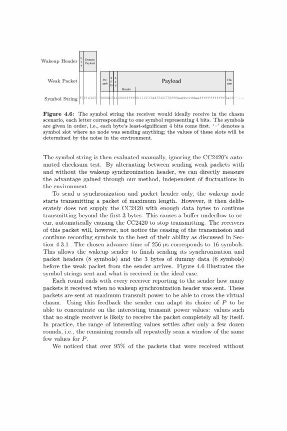
Wakeup Header

Weak Packet

Symbol String

Len

DummyPayload

Preamb

SFD

Len

Payload Chksum

f7214365--0000b7b16000ffff00112233445566778899aabbccddeeffffffffffff3a22--...

Header

Figure 4.6: The symbol string the receiver would ideally receive in the chasmscenario, each letter corresponding to one symbol representing 4 bits. The symbolsare given in order, i.e., each byte’s least-significant 4 bits come first. ‘-’ denotes asymbol slot where no node was sending anything; the values of these slots will bedetermined by the noise in the environment.

The symbol string is then evaluated manually, ignoring the CC2420’s auto-mated checksum test. By alternating between sending weak packets withand without the wakeup synchronization header, we can directly measurethe advantage gained through our method, independent of fluctuations inthe environment.

To send a synchronization and packet header only, the wakeup nodestarts transmitting a packet of maximum length. However, it then delib-erately does not supply the CC2420 with enough data bytes to continuetransmitting beyond the first 3 bytes. This causes a buffer underflow to oc-cur, automatically causing the CC2420 to stop transmitting. The receiversof this packet will, however, not notice the ceasing of the transmission andcontinue recording symbols to the best of their ability as discussed in Sec-tion 4.3.1. The chosen advance time of 256 µs corresponds to 16 symbols.This allows the wakeup sender to finish sending its synchronization andpacket headers (8 symbols) and the 3 bytes of dummy data (6 symbols)before the weak packet from the sender arrives. Figure 4.6 illustrates thesymbol strings sent and what is received in the ideal case.

Each round ends with every receiver reporting to the sender how manypackets it received when no wakeup synchronization header was sent. Thesepackets are sent at maximum transmit power to be able to cross the virtualchasm. Using this feedback the sender can adapt its choice of P to beable to concentrate on the interesting transmit power values: values suchthat no single receiver is likely to receive the packet completely all by itself.In practice, the range of interesting values settles after only a few dozenrounds, i.e., the remaining rounds all repeatedly scan a window of the samefew values for P .

We noticed that over 95% of the packets that were received without

3

16

28

27 24

23

3231

10

Figure 4.7: A subset of the wireless sensor node testbed we used for our practi-cal tests with three particular node triplets used for packet-in-packet experimentshighlighted. The second, stronger senders are indicated by thicker arrows.

a wakeup header were received completely without error. Effectively, if alink happened to be stable enough to receive the complete synchronizationheader, it also was stable enough to receive the packet completely withouterror 95% of the time. To reduce the filtering at the synchronization header,we decided to use a shorter preamble of only 2 instead of 4 bytes, shorteningthe synchronization header to 3 instead of 5 bytes. In the interesting trans-mit power range, this dramatically increased the number of packets receivedwithout a wakeup header, but lowered the ratio of packets received withoutany error to 0–25%.

4.4.3 Packet-In-PacketWe choose triplets of 2 sending nodes (B and I) and 1 receiving node (R),where node B will send the base packet and node I will send the injectionpacket. These triplets are selected such that at node R node I’s signalis at least 5 dB stronger than node B’s, to facilitate the capture effect.Further, we also ensure that node B’s link still has a high packet receptionratio (> 98%) in normal operation without packet injections. Finally, bothsenders should be able to hear the receiver for synchronization purposes. Ifnecessary we use the transmission power control options of the CC2420 toachieve this constellation. See Figure 4.7 for a few example triplets.

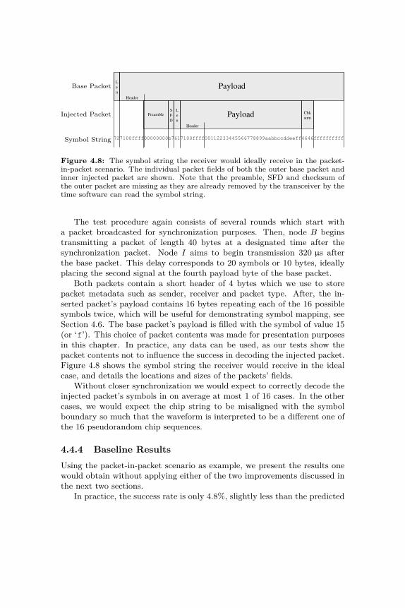
Base Packet

Injected Packet

Symbol String

Len

Payload

PreambleSFD

Len

Payload Chksum

727100ffff00000000b7617100ffff00112233445566778899aabbccddeeff4646ffffffffff

Header

Header

Figure 4.8: The symbol string the receiver would ideally receive in the packet-in-packet scenario. The individual packet fields of both the outer base packet andinner injected packet are shown. Note that the preamble, SFD and checksum ofthe outer packet are missing as they are already removed by the transceiver by thetime software can read the symbol string.

The test procedure again consists of several rounds which start witha packet broadcasted for synchronization purposes. Then, node B beginstransmitting a packet of length 40 bytes at a designated time after thesynchronization packet. Node I aims to begin transmission 320 µs afterthe base packet. This delay corresponds to 20 symbols or 10 bytes, ideallyplacing the second signal at the fourth payload byte of the base packet.

Both packets contain a short header of 4 bytes which we use to storepacket metadata such as sender, receiver and packet type. After, the in-serted packet’s payload contains 16 bytes repeating each of the 16 possiblesymbols twice, which will be useful for demonstrating symbol mapping, seeSection 4.6. The base packet’s payload is filled with the symbol of value 15(or ‘f’). This choice of packet contents was made for presentation purposesin this chapter. In practice, any data can be used, as our tests show thepacket contents not to influence the success in decoding the injected packet.Figure 4.8 shows the symbol string the receiver would receive in the idealcase, and details the locations and sizes of the packets’ fields.

Without closer synchronization we would expect to correctly decode theinjected packet’s symbols in on average at most 1 of 16 cases. In the othercases, we would expect the chip string to be misaligned with the symbolboundary so much that the waveform is interpreted to be a different one ofthe 16 pseudorandom chip sequences.

4.4.4 Baseline ResultsUsing the packet-in-packet scenario as example, we present the results onewould obtain without applying either of the two improvements discussed inthe next two sections.

In practice, the success rate is only 4.8%, slightly less than the predicted

727100ffff22222222d103132299992233445566770011aabbccddeeff889960600ff3ffcfcf727100ffff11111111c07202118888112233445566770099aabbccddeeff885757ffffffffff727100fffff77777777a6506077eeee7700112233445566ff8899aabbccddee3535fffffffff727100fffff6666666595475766dddd6677001122334455eeff8899aabbccdd2424fffffffff727100fffff77777777a6506077eeee7700112233445566ff8899aabbccddee3535fffffffff727100fffff5555555b423f6557c0ce56617d0911223346d829c58799aab70f1313fffffffff727100fffffd4d4444d03703ed4b7874d091f4b33447733f58199c3bbecff7b3b35fffffffff727100fffff66668816209e5b664444162d314e001149002f35775b6329064e02bffffffffff727100ffff11111111c07202118888112233445566770099aabbccddeeff885757ffffffffff727100fffffd4d4414d03703ed4b2b74d09112b338452f3596179657bec3ab93b35fffffffff727100ffff44444444ff2535444bbbb4556667700112333cddeeeff8899abb0202ffffffffff727100ffff33333333e2142433aaaa3344556677000122bbccddeeff8899aa71711fffffffff727100fffffeeeeeeee1f9cacee7552eecc88e9aa88f9dd6644006127334455acacfffffffff727100ffffdddddddd0fb9fedd8b88ddefff8d99a8bbffff8794a5ddecff889b9bffffffffff727100ffff22252522b7637f22f33332a644556657667bb12e6664e01604f366d6ffffffffff727100fffff66868666219e5b66b7b86550a1d800f1ee30eed5b7cb8279617eb209fffffffff727100fffff6666666695475766dddd6677001122334455eeff8899aabbccdd2424fffffffff

0 10 20 30 40 50 60 700%

50%

100%

Symbol Position

Succ

ess

Rat

e

base injected

Figure 4.9: Loose Synchronization, No Symbol Remapping. Sample and correct-ness rate on a per symbol basis.

116 = 6.25%. For intuition, examine Figure 4.9, which shows a representativesample of 17 received symbol strings. Every letter corresponds to a symbolin symbol transmission order, i.e., for every byte the 4 least-significant bitscome first. Unexpected symbol values are marked in blue. Since not asingle preamble was detected, all non-‘f’ symbols are classified as errors inthe body of the underlying packet.

It is easy to see the lack of tight synchronization in the variation of thefirst and last affected symbol of the underlying packet. However, a certainregularity in the erroneous symbols can be observed. In some cases, we canexploit this to salvage some of these scrambled lines, see Section 4.6.

At the bottom of Figure 4.9, the distribution of correctly received sym-bols can be found. The red line for the injected packet is almost completelyconstant at around 5% for the duration of the injection. This means, whenan injected packet’s preamble was correctly decoded, the remainder of thepacket was nearly always also completely without error. The uneven distri-bution of the base packet’s successes is caused by the varying densities of‘f’ symbols caused by the injection. This is due to certain of the injectedpacket’s symbols appearing to be more likely to be mapped to an ‘f’ thanothers. Finally, note the “tail” of the base packet sometimes experiencingsymbol errors even after the transmission injection has ceased.

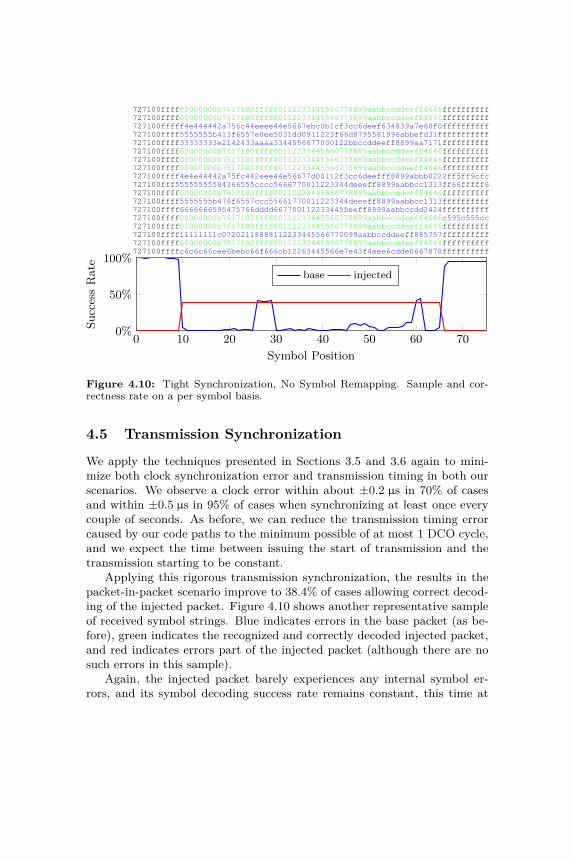
727100ffff00000000b7617100ffff00112233445566778899aabbccddeeff4646ffffffffff727100ffff00000000b7617100ffff00112233445566778899aabbccddeeff4646ffffffffff727100fffff4e444442a756c44eeee44e5667ebc0b1cf3cc6deef634839a7e60f0ffffffffff727100ffff5555555b413f6557e0ee5031dd0911223f66d8795581996abbefd31fffffffffff727100ffff33333333e2142433aaaa3344556677000122bbccddeeff8899aa7171ffffffffff727100ffff00000000b7617100ffff00112233445566778899aabbccddeeff4646ffffffffff727100ffff00000000b7617100ffff00112233445566778899aabbccddeeff4646ffffffffff727100ffff00000000b7617100ffff00112233445566778899aabbccddeeff4646ffffffffff727100ffff4e4e44442a75fc442eee44e56677d00112f3cc6deefff8899abbb0222ff5ff9cfc727100fff55555555584366555cccc5666770011223344deeeff8899aabbcc1313ff66fffff6727100ffff00000000b7617100ffff00112233445566778899aabbccddeeff4646ffffffffff727100ffff5555555b476f6557ccc55661770011223344deeeff8899aabbcc1313ffffffffff727100ffff6666666595475766dddd6677001122334455eeff8899aabbccdd2424ffffffffff727100ffff00000000b7617100ffff00112233445566778899aabbccddeeff4646c595c555cc727100ffff00000000b7617100ffff00112233445566778899aabbccddeeff4646ffffffffff727100ffff11111111c07202118888112233445566770099aabbccddeeff885757ffffffffff727100ffff00000000b7617100ffff00112233445566778899aabbccddeeff4646ffffffffff727100ffffc6c6c66cee6bebc66f666cb12263445566e7e43f4aee6cdde0667878ffffffffff

0 10 20 30 40 50 60 700%

50%

100%

Symbol Position

Succ

ess

Rat

e

base injected

Figure 4.10: Tight Synchronization, No Symbol Remapping. Sample and cor-rectness rate on a per symbol basis.

4.5 Transmission Synchronization

We apply the techniques presented in Sections 3.5 and 3.6 again to mini-mize both clock synchronization error and transmission timing in both ourscenarios. We observe a clock error within about ±0.2 µs in 70% of casesand within ±0.5 µs in 95% of cases when synchronizing at least once everycouple of seconds. As before, we can reduce the transmission timing errorcaused by our code paths to the minimum possible of at most 1 DCO cycle,and we expect the time between issuing the start of transmission and thetransmission starting to be constant.

Applying this rigorous transmission synchronization, the results in thepacket-in-packet scenario improve to 38.4% of cases allowing correct decod-ing of the injected packet. Figure 4.10 shows another representative sampleof received symbol strings. Blue indicates errors in the base packet (as be-fore), green indicates the recognized and correctly decoded injected packet,and red indicates errors part of the injected packet (although there are nosuch errors in this sample).

Again, the injected packet barely experiences any internal symbol er-rors, and its symbol decoding success rate remains constant, this time at

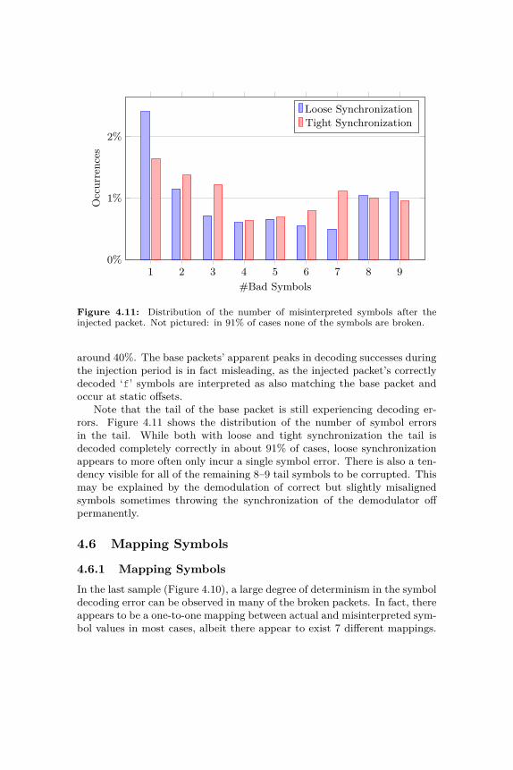
1 2 3 4 5 6 7 8 90%

1%

2%

#Bad Symbols

Occ

urre

nces

Loose SynchronizationTight Synchronization

Figure 4.11: Distribution of the number of misinterpreted symbols after theinjected packet. Not pictured: in 91% of cases none of the symbols are broken.

around 40%. The base packets’ apparent peaks in decoding successes duringthe injection period is in fact misleading, as the injected packet’s correctlydecoded ‘f’ symbols are interpreted as also matching the base packet andoccur at static offsets.

Note that the tail of the base packet is still experiencing decoding er-rors. Figure 4.11 shows the distribution of the number of symbol errorsin the tail. While both with loose and tight synchronization the tail isdecoded completely correctly in about 91% of cases, loose synchronizationappears to more often only incur a single symbol error. There is also a ten-dency visible for all of the remaining 8–9 tail symbols to be corrupted. Thismay be explained by the demodulation of correct but slightly misalignedsymbols sometimes throwing the synchronization of the demodulator offpermanently.

4.6 Mapping Symbols

4.6.1 Mapping SymbolsIn the last sample (Figure 4.10), a large degree of determinism in the symboldecoding error can be observed in many of the broken packets. In fact, thereappears to be a one-to-one mapping between actual and misinterpreted sym-bol values in most cases, albeit there appear to exist 7 different mappings.

Based on the symbols which were received at the location of the preambleof the inner packet we can identify which mapping took place. If we denoteby a the value of the preamble symbols and by s the correct symbol value,the 7 one-to-one mappings m(s, a) for 1 ≤ a ≤ 7 are:

m(s, a) = s− (s mod 8) + ((s+ a) mod 8)

We can exploit the bijectivity of these mappings to reverse them toreconstruct the original symbols in the majority of cases.

There are no simple one-to-one symbol mappings for the remaining casesof 8 ≤ a ≤ 15. This is easy to see when examining the pairs of symbols inthe payload of the injected packet not being recognizable as pairs anymore.However, it is likely that some information can still reliably be decoded, ascertain pairs of subsequent symbols should also follow an exploitable deter-ministic mapping, judging by the interplay of the predefined chip sequenceswhen time-shifted.

To detect injected packets after such a symbol mapping within the basepacket, we not only search for the synchronization word (preamble + SFD)as before, but also for the synchronization word with each of the 7 mappingsapplied. If one is found, the respective mapping is then used to decode thelength, payload and checksum of the injected packet.

4.7 Results

4.7.1 The ChasmThe wakeup synchronization header sent at maximum power by a closeneighbor unsurprisingly increases the number of cases in which any symbolswere recorded to essentially 100% (see Figure 4.12).

Figure 4.13 shows how often every symbol in the packet was receivedcorrectly at least once. For lower transmit power settings – emulating thecase of weak links – in the range from 7 to 10, corresponding to transmitpowers from -15 dBm to -10 dBm [75], our scheme raises the chance ofreceiving a complete copy of the packet from 5% to 30%. Without thesymbol remapping only 25% are achieved.

As the transmit power increases, regular transmissions without wakeupreach > 99% reliability. This is because frequently one of the receiversreceives a perfect copy of the packet by itself, while our approach still suffersfrom the penalties induced by using a mismatching synchronization header.Hence, we do not recommend using our approach for any and all links, butrather only for chasm-like scenarios in which only weak links are available.

Figure 4.14 shows the number of correct symbols received on averagewithin the transmit power setting range of 6 to 10 at each of the individual

NoWakeup WithWakeup0%

20%

40%

60%

80%

100%

Any

thin

gR

ecei

ved

Node 6Node 32Node 31Node 1

Figure 4.12: Percentage of received packets with and without the wakeup syn-chronization header at all 4 receivers of a test run.

3 4 5 6 7 8 9 10 11 120%

20%

40%

60%

80%

100%

Transmit Power Setting

Occ

urre

nces

No WakeupWakeup, No MappingWakeup, With Mapping

Figure 4.13: Percentage of cases in which at least 1 complete copy of the sentweak packet could be reassembled. Up to transmit power 10, our approach ofadding a wakeup synchronization header significantly improves the chances.

NW WW/NM WW/WM0

20

40

#Sy

mbo

lsR

ecei

ved

Cor

rect

ly Node 6Node 32Node 31Node 1

Figure 4.14: Average number of correct symbols received (out of 58) withand without the wakeup synchronization header at all 4 receivers of a test run.NW/WW = No/With Wakeup, NM/WM = No/With Symbol Mapping.

receivers. While the node with the best link (node 6) only gained about65% of additional correct symbols, overall the number of correct symbolsreceived more than doubled. As which symbols are correctly received for areceiver is independent of the other receivers (see Section 4.3.1), it standsto reason such an increase directly improves the chances of being able toassemble a complete correct copy of the packet.

The test run used for these plots contained 3800 samples, 3000 of whichwere taken within the transmit power setting range of 6 to 10.

4.7.2 Packet-In-PacketIn the packet-in-packet scenario, applying both techniques increases thesuccess rate for decoding the injected packet completely without error to64.3%. Tolerating up to 3 symbol errors, a success rate of 70% is reached.Figure 4.15 shows the same sample as in Figure 4.10, but with symbolremapping applied. It is easy to see that some of the erroneous lines frombefore have been corrected. However, in some instances a few symbols werecorrupted (marked in red). Peculiarly, judging from the success rate graphat the bottom, some locations in the packet are particularly prone to symbolerrors not following the mapping.

Figure 4.16 shows the distribution of the number of symbol errors inthe decoded injected packet given that its synchronization word was in-tact and recognizable. While the number of errors appears to be higher

727100ffff00000000b7617100ffff00112233445566778899aabbccddeeff4646ffffffffff727100ffff00000000b7617100ffff00112233445566778899aabbccddeeff4646ffffffffff727100fffff4e444442a756c44eeee44e5667ebc0b1cf3cc6deef634839a7e60f0ffffffffff727100ffff5555555b413f6557e0ee5031dd0911223f66d8795581996abbefd31fffffffffff727100ffff00000000b7617100ffff00112233445556778899aabbccddeeff4646ffffffffff727100ffff00000000b7617100ffff00112233445566778899aabbccddeeff4646ffffffffff727100ffff00000000b7617100ffff00112233445566778899aabbccddeeff4646ffffffffff727100ffff00000000b7617100ffff00112233445566778899aabbccddeeff4646ffffffffff727100ffff4e4e44442a75fc442eee44e56677d00112f3cc6deefff8899abbb0222ff5ff9cfc727100fff500000000b7611000ffff01112233445566778999aabbccddeeff4646ff66fffff6727100ffff00000000b7617100ffff00112233445566778899aabbccddeeff4646ffffffffff727100ffff5555555b476f6557ccc55661770011223344deeeff8899aabbcc1313ffffffffff727100ffff6666666595475766dddd6677001122334455eeff8899aabbccdd2424ffffffffff727100ffff00000000b7617100ffff00112233445566778899aabbccddeeff4646c595c555cc727100ffff00000000b7617100ffff00112233445566778899aabbccddeeff4646ffffffffff727100ffff00000000b7617100ffff00112233445566778899aabbccddeeff4646ffffffffff727100ffff00000000b7617100ffff00112233445566778899aabbccddeeff4646ffffffffff727100ffffc6c6c66cee6bebc66f666cb12263445566e7e43f4aee6cdde0667878ffffffffff

0 10 20 30 40 50 60 700%

50%

100%

Symbol Position

Succ

ess

Rat

e

Figure 4.15: Tight Synchronization, With Symbol Remapping. Sample andcorrectness rate on a per symbol basis.

0 1 2 3 4 5 60%

20%

40%

60%

80%

100%

#Bad Symbols

Occ

urre

nces

Loose, No MappingTight, No MappingLoose, With MappingTight, With Mapping

Figure 4.16: Distribution of the number of bad symbols within the injectedpacket once the injected packet’s preamble has been read correctly.

LS/NM LS/WM TS/NM TS/WM0%

20%

40%

60%

80%O

ccur

renc

es

Syncword foundAt most 3 symbol errorsAt most 0 symbol errors

Figure 4.17: Success rates for decoding the injected packets using the differenttechniques. LS/TS = Loose/Tight Synchronization, NM/WM = No/With SymbolMapping.

when applying symbol mapping, this is merely due to the fact that in thesecases additional synchronization words could be salvaged. These additionalinstances appear to be particularly prone to symbol errors, although the ex-tent is low enough to still preserve most of the packet data. Further, tightersynchronization appears to reduce the occurrences of these errors.

The total amount of recovered packets can be seen in Figure 4.17, sub-divided by the combination of applied techniques. Enforcing a limit on thenumber of symbol errors hurts the performance of the cases employing sym-bol remapping, as is to be expected. However, allowing up to 3 symbolerrors almost completely closes the gap to the number of cases in whichthe synchronization word of the injected packet was at all detected. Re-calling our injected packet being 46 symbols in length (when excluding thesynchronization word), an error of 3 symbols appears rather acceptable.

The test run used for these plots used the node triplet R = 23, I =24, B = 27 and contained 1900 samples for loose and tight synchronizationeach.


We explored the possibilities unfolding when mixing and matching synchro-nization headers and packet payloads as is made possible by inducing the

capture effect. Correctly interpreting the resulting sometimes jumbled sym-bol string is not trivial and certainly not as efficient as with a matchingsynchronization header. However, we showed that some scenarios may nev-ertheless profit: A) bridging a chasm which is only crossed by weak linksand may otherwise only be crossed taking a long detour – or not at all, if thenetwork graph is not connected otherwise, and B) propelling high-prioritypackets across a network without any waiting or any control message over-head, barely disturbing low-priority traffic. The resulting gains we observedin our experiments are best summarized by Figures 4.13, 4.14 and 4.17.

Integrating such new transmission primitives into existing systems andMAC layers will no doubt carry an additional overhead we did not have todeal with in our proof of concept implementations. Exploring the tradeoffsof such integrations promises to be an interesting topic for future work.

Although we conducted all our experiments using the IEEE 802.15.4standard, we believe these primitives to, in principle, be feasible in mostwireless standards which use temporally separated symbols for modulation.We also expect this style of communication to be able to benefit many otherscenarios beyond the two presented in this chapter.

The results of our solution to the chasm scenario undoubtedly leave roomfor improvements. One aspect worth further research is the use of multiplesenders, ideally synchronized well enough to cause constructive interferencein some subset of the receivers. Another promising direction is the use offorward error correcting codes to improve complete reception ratios at thecost of bandwidth. Such a scheme may also benefit the packet-in-packetprimitive.

We see the main application of the packet-in-packet primitive in enablinghigh-priority messages to be sent and received at almost any time, in spite ofongoing lower-priority transmissions. This significantly reduces the latencythese high-priority messages would otherwise incur, possibly accumulatingfurther at every hop. Another imaginable application are data aggregationalgorithms, using planned data insertions from many different nearby nodesto quickly form a single packet containing the aggregated data. To reducethe overhead of individual packets in this controlled scenario, one couldshorten the synchronization word and omit or shorten the checksum footer.

In the remaining failure cases, often some of the preamble symbols arerecognizable, but there is no reversible one-to-one symbol mapping. It maybe interesting to explore the interplay of the chip sequences defined by IEEE802.15.4 under varying degrees of desynchronization in future work. Webelieve that computing the original string of symbols no matter the timeshift is generally not possible. However, by smartly choosing the symbolcombinations used to carry the data of the injected packet, always retrievingall the data correctly may be possible. In the best case, this may even allow

dropping the stringent synchronization requirement at the cost of perhapsdoubling the injected packet’s length.

5Tempering Wireless Schedules

5.1 Introduction

Power control is the feature of some wireless transmitters to allow soft-ware to choose one of a selection of supported transmission powers for everytransmission made. Even though this feature has become widespread, mostwireless algorithms ignore its availability as it is often considered to in-troduce unnecessary complexity. We presented one example of a protocolbenefiting from power control in Chapter 2. In this chapter, we will considerthe problem of scheduling and examine how scheduling algorithms can bebenefit from power control. As a baseline we use the RAND algorithm [63].While simple in its greedy approach, RAND generally delivers good results.We chose RAND for both of those reasons, yet are able to improve uponmany of the characteristics of the schedules it produces significantly.

More generally, we find ourselves in the scenario of harnessing a singlefrequency channel using the IEEE 802.15.4 standard, i.e., we focus on timeand space division only. For medium access control (MAC) in this scenario,there are two general philosophies: opportunistic sending with backoffs andscheduling. With opportunistic sending, senders attempt to send as soon asa packet is ready to be sent. If the channel is busy, the attempt is repeatedafter a backoff period, until the transmission succeeds. Opportunistic send-

79

ing incurs little to no overhead if traffic is low, but as traffic increases, itbecomes increasingly inefficient and transmission delays become more andmore unpredictable.

Scheduling on the other hand divides time into slots and assigns trans-missions to slots such that all transmissions in each slot can be carried outsimultaneously. Hence, collisions can be completely avoided and transmis-sion latency becomes deterministic. This comes at the cost of flexibility asevery update to a schedule may incur significant computation and dissemi-nation overhead. Such updates are often necessitated by fluctuating trafficlevels and changing environment conditions. Mechanisms to reclaim someof the flexibility have been proposed, such as slot stealing [42] and switch-ing between opportunistic sending and schedules on-the-fly [65]. For ease ofanalysis, in this chapter we will assume the traffic pattern to be static andknown in advance. Without loss of generality we can assume each trafficflow to have the same desired bandwidth and to flow from one node to animmediate neighbor. The quality of a schedule may then be defined by thenumber of slots required to service all traffic flows once: the shorter theschedule, the more often the schedule can be repeated in any given timeframe, which directly correlates with the network’s overall throughput.

By employing a model for the probability of a set of transmissions suc-ceeding simultaneously, it is possible to efficiently predict viable slots offlinewithout the need to try them first. This allows the creation of schedulesoptimized to make use of the medium to the fullest possible extent in eachslot. The Signal-to-Interference-plus-Noise-Ratio (SINR) model is one ofthe most established models for this purpose, e.g., [26]. It posits that, ifthe ratio between a signal’s power and the sum of the remaining signals’powers plus the noise floor clears a certain threshold at a receiver, then thatsignal may be correctly decoded at that receiver. There are different ways toobtain the variables required by this model, the gain matrix of the networkand the noise vector: measuring the noise floor comes almost for free, butmeasuring link gains accurately usually requires actually sending packets.For the most accurate measurements, these packets should be sent withoutinterfering traffic, which implies sacrificing regular transmissions slots. Lessaccurate but more subtle methods of measurement making use of knowl-edge about regular traffic failing or succeeding may be preferable in somecircumstances.

The strength of each arriving signal – as well as the interference it causes– depends on two variables: (1) the gain of the link, and (2) its originaltransmission strength. Hence, there are in fact two fundamental questionsthat any scheduling mechanism needs to answer: who sends when, and whosends how strongly. In practice, the second question is often trivialized:having every sender use its maximum transmission power optimizes the

TA TB TC RC RB RA

Figure 5.1: The “sandwich”: an abstract geometric example of a scenario inwhich the use of individual transmission powers for each link reduces schedulelength considerably. At equal transmission powers, all 3 links need to be scheduledin separate slots, while sensible power control allows scheduling all 3 links in thesame slot.

signal quality at the receiver. This also reduces the task of computing aschedule to the combinatorics of finding a preferably small amount of slotsable to serve all desired links.

However, power control is now widespread in hardware. Theory work inthis area has long proven this option to provide significant benefits: in somesituations significantly shorter schedules servicing the same traffic can befound [58]. Figure 5.1 shows a simple geometric example, in which powercontrol allows shortening the schedule by a factor of 3. While such anexample goes counter to intuition, log-distance path loss allows for suchconfigurations when powers and distances are chosen carefully.

Unfortunately, realizing the algorithms and techniques proposed by the-ory is typically unrealistic. For example, in practice, the possible transmis-sion power values each sender may choose from are usually bounded to acertain range and are not arbitrarily fine-grained. Yet, these concerns arenot addressed by the theory community.

As a result, the real world usually ends up using simple heuristics tocompute schedules while ignoring the opportunities offered by power control.For example, Z-MAC [65], as well as the RAND algorithm it is partiallybased on, only consider the maximum transmission power. We feel that,when choosing to take on the burden of the overhead associated with ascheduling approach, to not also incorporate power control is a waste.

In this chapter, we propose a practical algorithm to compute tempered(hardened) schedules harnessing power control: by using tempered (lowered)transmission powers, we can reduce the unneeded interference caused bytransmissions. On average, this allows us to pack more links into a singleslot than possible at maximum transmission power. Our results show thatwe are consistently able to schedule the same set of links in 20–25% fewerslots than possible without power control. That is equivalent to a 25–33%increase in overall throughput of the network.

Further, we can make use of our reduced interference levels to packlinks into the schedule a second time at no additional cost. By scoringsecond schedulings of links a fraction of their first schedulings, we are ableto quantify the additional value provided by a schedule without impactingits length. Schedules not employing power control also benefit from thisruling. However, our schedules profit more so, achieving a comparativelyhigher total score per slot value.

Additionally, we address the problem of the environment, i.e., the gainmatrix, changing over time. This is a common problem in practice: doorsmay open or close, the temperature and humidity may change, people tendto move around. A schedule computed for one version of the gain matrixmay turn obsolete within minutes as some links cannot be served anymore.By increasing the power of a link that was predicted to work but failed, weare in many cases able to salvage slots without having to move links to otherslots or recomputing the schedule.

All our schedules are verified on a testbed of wireless sensor nodes de-ployed in an office building offering a typical noise background and dynamicenvironment. Experiments confirm that the improved schedules are just asreliable as traditional full power schedules. Both kinds of schedules sufferfrom up to 5% of the links failing to successfully transmit, depending onthe chosen minimum SINR threshold for the admissibility of links. Thisis mainly due to these links being mispredicted on basis of a changed gainmatrix.

5.2 Related Work

To avoid transmission collisions while also maximizing the possible through-put of a wireless network, numerous techniques and protocols have been pro-posed. The most important approaches can be grouped into time division(TDMA), frequency division (FDMA), space division (SDMA) and code di-vision (CDMA). In this chapter, we focus on harnessing a single frequencychannel and restrict ourselves to the IEEE 802.15.4 standard [32], i.e., wefocus on time and space division. However, our solutions may be general-ized to deal with multiple available frequency channels, and we believe theresults to apply to a majority of today’s wireless standards.

Various collision prediction models have been proposed and used in thepast. The simplest models abstract the network into a communication graphin which every pair of nodes is connected by an edge if and only if they areable to communicate directly. A collision occurs if more than 2 neighborsare sending simultaneously. This model is used, for example, by schedulingalgorithms such as RAND [63] and its derivatives. This model works best

in homogeneous networks, i.e., networks in which all edge gains are verysimilar.

In practice, so called physical models, such as the SINR model, have beenproven to be very accurate [2,25,26,56]. These models typically require es-timations of the signal strength fall-offs between two nodes, called gains. Ifthe network geometry is known, these gains may be computed directly as-suming, for instance, a log-distance path loss. This approach suffers greatlyfrom irregularities in the environment as well as multi-path effects. Alter-natively, each of the entries of the gain matrix may be determined throughmeasurements. This carries with it a certain overhead – at the minimum,in several short slots, each prospective sender needs to send alone once. Inthis chapter, we valued the accuracy gained by the latter method more thanthe avoided overhead, as we were interested in estimating the maximumpotential improvements possible through power control. However, based onthe experiences we had with our experiments, we are able to suggest severalways to reduce the impact of this overhead in practice (see Section 5.8).

A framework for computing schedules avoiding collisions was proposed byRamanathan [63]. In the same work, the RAND algorithm was introduced.Its basic idea is to iterate over the links to be scheduled in a random orderand add them to the first slot able to accommodate them. If no slot issuitable, an additional slot is appended to the schedule. In spite of thealgorithm’s greedy nature, by taking the best outcome of multiple runsyields a consistently decent performance. One major advantage of RANDis its efficiency, which it gains by dropping all pretenses of attempting toguarantee an optimal solution or an approximation thereof. We will discussthis greedy bin packing algorithm in more detail in Section 5.5, Algorithm 2.

Rhee et al. [66] later provided a distributed version called DRAND withcomparable performance to RAND. DRAND works by negotiating slot usagelocally in each node’s 2-hop neighborhood. This makes it especially wellsuited for larger networks as no global coordination is required. The popularZ-MAC protocol [65] uses DRAND as scheduling algorithm during phasesof high load in the network.

Both RAND and DRAND assume transmission powers to be constant.In certain denser networks, choosing a different global transmission power(less than the maximum power) may already drastically improve these algo-rithms’ performance. However, actually adding a transmission power vari-able for every link to these algorithms is a problematic proposition as “2-hopneighborhood” then turns into a rather fuzzy concept. ElBatt et al. [14] pro-posed enhancing schedules with power control similar to our work. However,they did not perform any practical evaluation of their heuristics.

In the last decade, power control has also received a lot of attention fromthe algorithmic networking community, starting with the work of [56].

The first algorithmic result to schedule an arbitrary link set was byMoscibroda et al. [58]. This result was soon superseded by the first approx-imation results [4, 24]. These early approaches involved (directly or indi-rectly) partitioning links into length groups, which results in performanceguarantees that are at least logarithmic in ∆, the so-called link diversity, i.e.,the ratio between the longest and the shortest link [5, 10, 24, 27]. However,link scheduling cannot be solved optimally, as NP-hardness was establishedin [24]. This is the reason why our algorithm is also heuristic in nature, anddoes not try to solve the problem “optimally”. A breakthrough paper onthe theory side was by Kesselheim [35], who discovered the first schedulingalgorithm that uses power control with logarithmic approximation guaran-tees.

On the positive side, theoreticians established that – in theory – powercontrol is in fact powerful. There are instances with n links that can bescheduled in a single slot with power control, while, without power control,all n links need to be scheduled sequentially [58]. This result can evenbe generalized to the case when we compare arbitrary power control toso-called oblivious power, where the power of a link only depends on thelength of the link [17]. However, the networks which yield these boundsare extremely cooked up, they can only be witnessed in a “theory zoo” butcertainly not in the wild. Sometimes the lengths of links must grow doublyexponentially [27, 28] in order to prove the theorem.

There has been some work that showed that power control can be effec-tive in practice. For example, Lin et al. [47] proposed a feedback mechanismto balance out the quality fluctuations of individual links. In contrast to ourwork, these earlier papers again do not consider realistic networks. In anearly effort, Moscibroda et al. [57] showed that power control can increasethe throughput in a wireless sensor network with link diversity ∆ = 3 by afactor of 3. In fact, they proved the “sandwich” situation shown in Figure 5.1to be feasible in practice.

5.3 Link Model

The link model is concerned with providing accurate and up-to-date linkstate information, such as a link’s current gain and the noise floor at areceiver. It forms the basis for estimating link set success probabilities inthe prediction model. While the physical locations of the nodes are readilyavailable to us, we do not attempt to infer link gains from such data, assuch approaches are fraught with inaccuracies, especially in complex indoorenvironments. Instead, we perform measurements using the same deviceswe will later use to verify the viability of schedule slots. Such a method is

3 7 11 15 19 23 27 31

−20

−10

0

Transmission Power SettingRed

uctio

nin

Rec

eive

dSi

gnal

Stre

ngth

[dB

]

data sheet values

Figure 5.2: Relative received signal strengths plotted against the different trans-mission powers for a few different links.

not only convenient to integrate into the regular operation of just about anyexisting wireless network, it also yields measurement values which should inmost cases match the performance in regular operation later on.

First, we attempted measuring only the achieved received signal strengthsat the highest possible transmission power settings for every link. As a re-duction of the transmission power by some factor x should also reduce thereceived power by the same factor x, we hoped to be able to infer the receivedsignal strengths for other transmission power settings from this one mea-surement per link. Unfortunately, in many cases, the different transmissionpower values specified in the data sheet differed from what was measuredin practice. Figure 5.2 shows the reduction in measured received transmis-sion power compared against the case of maximum transmission power (onthe vertical axis) plotted against the used transmission power settings (onthe horizontal axis). The dashed line indicates the values as given by theCC2420’s data sheet [75]. Each of the other lines represents the averagevalues measured for a different single link repeatedly sampled over the spanof 1 hour. The shown links were chosen to showcase some of the differentkinds of discrepancies we encountered.

Figure 5.2 makes it clear that measuring the link gains only at the maxi-mum transmission power and extrapolating the gains for other transmission

powers is certain to incur up to 1–3 dB of error on average, i.e., up to afactor of 2 in absolute signal strength. As these curves are somewhat char-acteristic for individual links, often changing only marginally if sampled onsuccessive days, one option is to measure them once and then only updatethe gain of the maximum transmission power frequently. As can be seenfrom the varied shapes of the curves, adding just one or two additional mea-surements is not sufficient to accurately determine a link’s curve. Hence, inthe interest of accuracy, we chose the most detailed option: measuring allpoints of the curves every power test. However, as that requires 15-times asmany measurements as the extrapolating option, we expect that one wouldtry to find a more reasonable tradeoff in practice.

This essentially adds a third dimension to our gain matrix, which is thusnow parameterized by sender, receiver and transmission power. This linkmodel turned out to work well at night, i.e., when the environment wasalmost static as the office building was empty. In contrast, during officehours, even a few fluctuating links caused a large portion of the generatedschedule slots to be too unreliable for use. This is due to the fact thatunderestimating a link often ruins all slots it appears in: not only is thelink afforded unneededly little interference at its receiver, but the otherreceivers also expect the link to cause far less interference than it actuallydoes. Figure 5.3 shows the received signal strength over the course of 1 hourduring office hours for a few select links. Signal strength jumps on the orderof 5 dB in either direction between 2 or 3 consecutive measurements (2–4minutes in our setup) are not uncommon.

To deal with these fluctuating links we decided to have the link modelnot only keep the most recently measured gain matrix, but also keep severalolder versions in memory. We now offer 2 values for each link to the predic-tion model: a signal gain and an interference gain. The signal gain of a linkis the lowest of the gain values for that link amongst the kept gain matrices;analogously, the interference gain is the highest value. This pessimisticallydrops the peaks in Figure 5.3 for the signal value, and fills the dips for theinterference values, effectively smoothing out the fluctuations. As retentiontime for old gain matrices we found 15 minutes to be reasonable in our case.This value should be chosen according to the power test frequency such thatrecent peaks and dips are likely to be found and remembered.

In addition to link gains, the link model also collects noise floor mea-surements for every node. These values serve two purposes: to deduct thenoise component from measured received signal strengths, and for use inpredictions in the SINR formula as additional interference source. In ourtestbed the noise is negligibly small (< −95 dBm) for most nodes, but notfor all. Further, not subtracting the noise component from signal strengthscan accumulate to a large error in predictions for slots with a large number

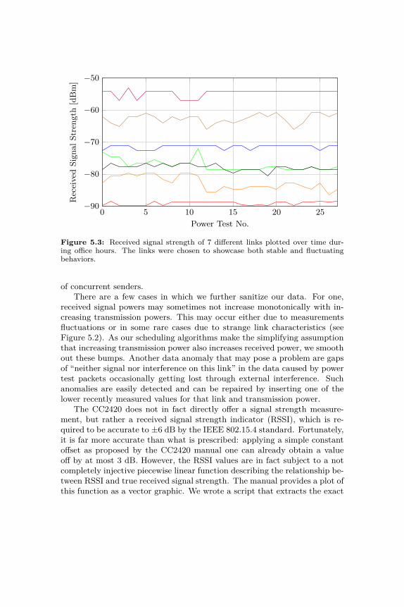
0 5 10 15 20 25−90

−80

−70

−60

−50

Power Test No.

Rec

eive

dSi

gnal

Stre

ngth

[dB

m]

Figure 5.3: Received signal strength of 7 different links plotted over time dur-ing office hours. The links were chosen to showcase both stable and fluctuatingbehaviors.

of concurrent senders.There are a few cases in which we further sanitize our data. For one,

received signal powers may sometimes not increase monotonically with in-creasing transmission powers. This may occur either due to measurementsfluctuations or in some rare cases due to strange link characteristics (seeFigure 5.2). As our scheduling algorithms make the simplifying assumptionthat increasing transmission power also increases received power, we smoothout these bumps. Another data anomaly that may pose a problem are gapsof “neither signal nor interference on this link” in the data caused by powertest packets occasionally getting lost through external interference. Suchanomalies are easily detected and can be repaired by inserting one of thelower recently measured values for that link and transmission power.

The CC2420 does not in fact directly offer a signal strength measure-ment, but rather a received signal strength indicator (RSSI), which is re-quired to be accurate to ±6 dB by the IEEE 802.15.4 standard. Fortunately,it is far more accurate than what is prescribed: applying a simple constantoffset as proposed by the CC2420 manual one can already obtain a valueoff by at most 3 dB. However, the RSSI values are in fact subject to a notcompletely injective piecewise linear function describing the relationship be-tween RSSI and true received signal strength. The manual provides a plot ofthis function as a vector graphic. We wrote a script that extracts the exact

data points from this graphic, and manually smoothed out the non-injectiveparts of the function to be able to create a reverse mapping. Chen et al. [7]explored this mapping in far greater detail, but our simple approach seemedto work well enough in practice.

The set of transmission power settings we use in all experiments in factexceeds the set described in the manual: the manual lists 8 possible set-tings (3 through 31 in steps of 4). We use 7 additional setting values, eachbetween two of the listed values, for a total of 15 power setting values (3through 31 in steps of 2). Considering more power settings naturally im-proves the flexibility of algorithms employing power control. We tested theremaining possible power settings (the even values) but found them to al-most always result in power outputs identical to adjacent power settings.These undocumented power settings were also examined by Maheshwari etal. [51]. However, we were unable to reproduce any successful transmissionsusing power settings below 3.

5.4 Prediction Model

A (schedule) slot can be defined as set of tuples of transmitting node, re-ceiving node and transmission power. In our scenario we expect every nodeto appear at most once in a slot, either as sender or as receiver, but thisassumption may be weakened: When considering broadcast transmissions,multiple tuples may have the same sender. Further, full-duplex radios allowa node to appear in a tuple as receiver even if it also appears in tuples assender.

Given a slot, the goal of the prediction model is to make as accurate of aprediction of the outcome as possible – without trying the slot in practice.In particular, we are interested in whether each of the links in the slot islikely to work, i.e., have a success probability p > pthreshold. We call suchslots feasible.

For our purposes we chose the SINR model, fed with measurements ofevery link’s received signal power at every transmission power (the linkmodel).

The slot is given by link set L = {l1, . . . , lk} = {(t1, r1, p1), . . . , (tk, rk, pk)},the lowest and highest (see Section 5.3) recent received signal powers for alink la are denoted by s(la) and i(la) respectively, and the noise floor at noder by n(r), then our SINR model states that a link la ∈ L is able to transmitsuccessfully if and only if the following equation holds at the receiver:

−4 −2 0 2 4 6 8 10 12 140%

20%

40%

60%

80%

100%

SINR [dB]

Succ

ess

Rat

io

Figure 5.4: Scatterplot of link success ratios split into SINR buckets of 0.25 dBeach. Colors indicate which of the 3 experiments the value came from.

SINR(la) = s(la)∑lb∈Llb 6=la

i(lb) + n(la)> β

Here β is the so called SINR threshold, which needs to be cleared by thesignal-to-interference-plus-noise-ratio (SINR). Unfortunately, in reality linksuccess is not as black and white as the formula suggests: between a “highenough” and a “too low” SINR there exists a transition region in which thepacket reception ratio gradually tapers off.

To decide on a fitting β we conducted an experiment, in which we com-puted a schedule at the start and then tested that schedule’s slots repeatedlyfor about an hour, ignoring changes in the environment. We then dividedthe results for all tested links into buckets based on the SINR we computedfor the link beforehand. Figure 5.4 plots the ratio of successful links foreach bucket, each bucket 0.25 dB in size. The results from 3 experiments,each with a different schedule, are shown, in a different color each. Theexperiment in blue used different parameters for the schedule computation,which should not be of interest for this discussion.

While in the blue test run the success ratio rather quickly increases fromaround 0% to 80% for SINR values from 0 dB to 2 dB, the other test runs

experience a significantly wider transitional region. The red test run evenconsistently reaches a packet reception ratio of almost 10% at SINR valuesbelow 0 dB, i.e., when the quotient is below 1 as the interference and noisewas measured to be stronger than the signal.

We explored computing a piecewise linear function mapping SINR tosuccess probability. However, as this mapping appeared to vary dependingon external parameters (such as the slots used and perhaps the environ-ment), especially in the interesting area of 2 dB < SINR < 10 dB, anymapping function procured from such experiments was doomed to be tooinaccurate to be used for a subsequent experiment. Our main takeawayfrom these experiments is that the SINR model and/or our measurementsare too inaccurate as to be able to guarantee a successful reception at lowvalues of β.

For computing schedules, we decided that we were interested only inslots, in which all links had a success probability of at least 80%. Based onour findings above we forewent a SINR-to-probability mapping function andsettled for using hand-picked constant values for β. As we are ultimatelyinterested in computing schedules that are viable in practice, we tuned themodel parameters to make the model decide pessimistically, i.e., focus onavoiding false positives (links predicted to work not working) at the cost ofan increased amount of false negatives (links predicted to not work working).For exploiting links with a success ratio in the transition region we refer toother works specializing on this topic such as the work by Maheshwari etal. [51].

Reasonable but pessimistic values for β lie in the range of 6–12 dB:for a link to successfully invoke the capture effect to be heard over theinterference from the other senders in the slot requires exceeding the theircombined power by 2–8 dB, depending on various factors such as the numberof interfering signals [51, 78] (see also Section 3.7.2). In addition, we haveseen that the link qualities can easily spontaneously fluctuate by 2 dB inthe most static phase of our environment, up to 5–6 dB in an active phase.

5.5 Tempering RAND

The input of a scheduling algorithm is a set L of links representing thetraffic to be served. Without loss of generality we can assume all trafficdemands to be between two neighboring nodes and of unit size: to solvethese more general cases, we can split every traffic demand into multipletraffic demands of unit size (L now becomes a multiset) and split traffic be-tween non-neighboring nodes into multiple single-hop traffic demands usinga suitable routing algorithm. For our experiments we chose L to include all

Algorithm 2: RANDData : Function Feasible(S)Input : Links LOutput: Schedule (set of slots (sets of links))C← {}while L 6= {} do

l← random element from LL← L \ {l}foreach S ∈ C do

S’← S ∪ {l}if Feasible(S’) then

C← C \ S ∪ S’break

if l could not be added to an existing slot thenC← C ∪ {{l}}

return C

feasible links, i.e., all links that are able to successfully transmit alone atmaximum transmission power.

A valid output of a scheduling algorithm is a set C of sets of links calledslots. The union of all slots must be L, and all slots must be feasible, i.e.,all links within the slot must be able to transmit successfully concurrently.In the case of a scheduling algorithm not using power control, it is implicitthat all links are to be used at full transmission power. When using powercontrol, the algorithm additionally needs to return the powers to be usedfor the individual links within each slot.

The classic RAND algorithm was a special case in the general schedulingframework proposed by Ramanathan et al. [63]. Pseudocode for RAND isgiven by Algorithm 2: the input links are greedily added to existing slots ina random order. If no existing slot is able to accommodate the next link,a new slot is added. The algorithm’s convincing features are its simplicityand efficiency in practice, defying the combinatorial nightmare that NP-hard scheduling [24] poses. RAND’s consistency can be slightly enhanced byrunning it multiple times and choosing the best output among the instances.

As our algorithm builds upon the basic structure of RAND, it can reapthe same benefits: links are considered in a random order and greedilyassigned a slot. All links assigned to a slot also carry a transmission powersetting. Initially, when the first link is added to a slot, its power setting is setto the minimum for which the link is feasible. When another link is addedto a slot, the existing links of the slot may need to raise their power settings

Algorithm 3: PowerRANDInput : Links LOutput: Schedule with transmission powers (set of slots (tuples of

sets of links and power mapping))C← {}while L 6= {} do

l← random element from LL← L \ {l}foreach (S, p) ∈ C do

S’← S ∪ {l}p’← FindPowers(S’)if p’ 6= ∅ then

C← C \ (S, p) ∪ (S’, p’)break

if l could not be added to an existing slot thenC← C ∪ {({l},FindPowers({l}))}

return C

Algorithm 4: FindPowersData : Available transmission power settings PData : Function Predict(L, p) returning working linksInput : Links LOutput: Map: link → transmission power; or ∅foreach l ∈ L do

p[l]← min Prepeat

change← Falseprediction← Predict(L, p)foreach l ∈ L do

if l /∈ prediction thenif p[l] = max P then

return ∅else

p[l]← min {x ∈ P | x > p[l]}change← True

until change = Falsereturn p

to account for the interference caused by the new link. If a link’s powersettings cannot be raised far enough to enable the new link, the new linkcannot join the slot as it would otherwise become infeasible. We abstractedthe process of attempting to find an agreeable set of power settings for apotential updated slot into a subroutine called FindPowers. The completepseudocode listings are given by Algorithms 3 and 4.

After computing a schedule with our algorithm, it may be beneficialto optimize the individual slots: as each slot’s power settings are as low aspossible to allow for as much room as possible for potential further links, theSINR values of the individual links are likely not as high as they could be.Now that we know that no further links will be added to the slot, we maygain an overall “better” slot by raising the power settings. We define a set ofpower settings for a slot to be better than a different set of power settings, ifthe minimum SINR value it induces amongst the links of the slot is higher.In a stable environment, such increases in SINR values are not worth much(at least with the modulation prescribed by our chosen wireless standard),but as we are dealing with an environment in which links may suddenly andabruptly change, delivering more interference or a weaker signal, using anyavailable additional buffer is prudent.

Exhaustively searching for the optimal power settings for a slot is nottenable in practice, especially for slots containing 5 or more links. Instead,we start at a random position in the space of reasonable power settings,i.e., we set every power to a value between the minimum suggested by thescheduling algorithm and the maximum possible, and then follow the gradi-ent of the quality to its local maximum, where the quality of a set of powersettings is defined as the resulting minimum SINR value among the links.We repeat this process for 50 different random starting values and use thelocal minimum with the best quality we found. Comparing the achievedquality to that of the exhaustive search for a several random samples, wefind our gradient method to get sufficiently close to the optimum in mostcases.

Without specifically giving scheduling algorithms an incentive to ensureall slots are utilizing the available medium well, the schedules they producemay contain slots containing only one or two links – not because these linksmake scheduling additional concurrent links impossible, but because all linksthat could be added are already being served in other slots. Such schedulesare wasteful in practice.

Hence, to perform our experiments with realistic schedules, we decidedto allow the scheduling algorithms to schedule any link a second time ata reduced reward. More concretely, we implemented the following scoringfunction for a schedule C that is supposed to cover L:

Score(C,L) =

0 if ∃l ∈ L : |{S ∈ C | l ∈ S}| = 0∑l∈L

LinkScore(C,l)

|C| otherwise

LinkScore(C, l) =

1 + ε if |{S ∈ C | l ∈ S}| ≥ 21 if |{S ∈ C | l ∈ S}| = 10 otherwise

In practice, we chose ε = 1/4, i.e., 4 secondary schedulings are equiv-alent to 1 primary scheduling. This scoring approach can be seen as ageneralization of the previous quality measure (the schedule’s length) usingan arbitrary LinkScore function: when setting ε = 0, the resulting schedulescore would induce the same quality ordering on schedules as their length(or rather: shortness).

We extended both RAND and PowerRAND to create schedules targetingthe new scoring function. The extension applies to both algorithms thesame: Once the set of remaining links (L) is depleted, we replenish it onceand continue the algorithm. Hence, at the end, every link is contained in theschedule twice. We then return a schedule consisting of the oldest k slotsfor the k that maximizes the schedule score for those slots (this requires theslot set C to preserve an ordering, which is not reflected by the pseudocodegiven above). If additional link score is awarded for a third scheduling of alink, one would need to replenish L a second time, and so on. We found thedifference between rewarding only the second scheduling and additionallyrewarding a third scheduling to be negligible in practice. However, theabove algorithm and scoring achieve the desired effect of smoothing outthe produced schedule such that all its slots appear to utilize the mediumreasonably efficiently. Note that, even though we allow for our algorithmsto add slots in this process, the choice of the scoring function makes thecircumstances required for a slot addition virtually impossible.

Power control does not only afford us more efficient schedules, it also al-lows us to react swiftly to a slot ceasing to work, for example, due to changesin the environment. More specifically, if one link within a slot fails to trans-mit repeatedly, one may edit the schedule on-the-fly and increase that link’stransmission power for that slot by a notch. This technique particularlybenefits from larger minimum SINR values (larger β) as the additional in-terference caused by the attempt to repair one link is unlikely to disturb theother links. As we are dealing with a particularly active environment in ourscenario, we found this technique to be helpful in offsetting the fluctuationsand thus prolonging the applicability of a schedule.

Figure 5.5: The floor plan and node layout of the wireless sensor node testbed weconducted our experiments on. We tested a smaller and a larger set of nodes. Thesmaller one only includes the nodes in red, the larger one also includes the nodes inblue. The node with the thick border was used as starting node for synchronizationwaves for both node sets.

Another attempt we made to fight the fluctuating link qualities was toadd slots of a certain minimum size which worked well to a whitelist, to beautomatically grandfathered in into schedules generated in the future. Sim-ilarly, we added slots that turned out to not work as expected to a blacklist,forbidding that combination of links to be used by a future schedule. Neitherof these methods were particularly successful: whitelisting, while it may findand preserve particularly good link combinations by chance, is not immuneagainst changes of links within the whitelisted slots, and blacklisting is ahopeless proposition in face of the myriad of possible combinations of links.


All our experiments were conducted on FlockLab with TelosB motes. As thetestbed consists of installations on the walls of an office building, the activityof the people using this office building, such as office doors being openedor closed and people moving about, creates a dynamic environment. Sucha real world scenario allows us to experience and address problems usuallynot present in lab setups. Figure 5.5 shows the floor plan and node layoutof the testbed. All nodes were located on the same floor of the building.

To ensure that possible collisions in a schedule slot are not avoided dueto a lack of synchronization, we periodically synchronize all nodes to a previ-

ously chosen central node of the network, which is at most 3 hops from everyother node (see Figure 5.5). As synchronization period we found 11 secondsto be an adequate value for our experiments. This keeps our synchronizationerror below ±2 µs at all times.

Further, we take special precautions that no node misses its scheduledtransmission time: 30 ms before the transmission time is reached we starta series of busy waits on the separate parts of the target timestamp (seeSection 3.6). We find that over 99.9% of our transmissions are started within±50 µs of the correct local time. For reference, the packets we transmit areabout 2 ms in length. Hence, even if added up these two error sourcesand included the propagation delay of up to ±0.34 µs (accounting for upto 100 meters difference in path lengths), any two packets sent within inthe same slot are guaranteed to temporally overlap at the receiver for atleast 2000µs−52.34 µs or over 97% of the packet. We deem this sufficientfor obtaining meaningful results about the feasibility of schedule slots.

To coordinate the experiment, we make use of a feature offered by Flock-Lab which allows us to remotely receive and send serial input to nodes viaa TCP connection each. We have a coordinator script running on a regularx86-64 desktop machine, connecting to each of the nodes to issue only veryloosely synchronized commands. Such a central coordinator is an uncom-mon feature in real world wireless networks. However, it vastly simplifiesresult gathering, timely schedule computation and command dissemination.These tasks are not the focus of our work – we are more interested in aproof of concept and measurement of the physical feasibility of schedulesemploying power control. Our current setup essentially has the centralizedcontrol flair of popular software defined networks.

Our experiments contain 3 kinds of phases of operation:

• Synchronization phases to align node clocks to be able to enforcepacket collisions as described above.

• Power test phases to obtain measurements for the values of the gainmatrix.

• Set test phases to try out simultaneous use of a certain set of (sender,receiver, transmission power) triplets, i.e., test a schedule slot.

Each of these phases is subdivided into a number of time slots, eachlasting 1/8 of a second (not to be confused with schedule slots). Synchro-nization phases start by the central node of the network being woken bythe coordinator. This node’s clock will serve as the global reference clockamongst the nodes. Woken nodes will broadcast their time at maximumtransmission power at the start of each slot with a probability of 1/3, or

with a probability of 1 if have not transmitted since being woken. Nodesimplicitly gain a parent node – the node whose broadcast woke them. Inthis phase, they will continue accepting timestamps from their parent node,should it transmit again. To minimize the error incurred each hop, we applythe techniques detailed in Section 3.5. Each synchronization phase lasts for10 time slots, i.e., 1.25 seconds.

In a power test phase, one node after the other will transmit once ateach available transmission power level. The packets being sent containboth the sender’s ID and the transmission power that was used. Whenevera node successfully receives a packet during this phase, it will note senderand transmission power as well as the received signal strength indicator(RSSI) and pass them on to the coordinator via serial output. I.e., once apower test phase is complete, the coordinator will have collected sufficientdata to create a fresh complete snapshot of the gain matrix. Also in thisphase, noise floor levels are measured several times by all nodes. To avoidoutliers due to other transmissions in the environment, all but the lowest ofthe measured noise floor values are discarded. To construct the gain matrix,the coordinator first converts the RSSI values into more accurate receivedsignal strength values (see Section 5.3) and then subtracts the measurednoise floor values for the respective receivers. We run power test phasesonce every 2 minutes.

In a set test phase, the coordinator chooses a slot of a computed scheduleand puts it to the test in practice: all transmitting nodes of the slot areinformed of their duty as well as their transmission power for this scheduleslot. Due to the loose synchronization between coordinator and nodes, thecoordinator picks a time slot which lies 2 slots (0.25 seconds) in the futureto ensure all transmitting nodes can prepare and agree on the same timeslot. All non-transmitting nodes record which sender’s packet they receive– if any at all – and report this to the coordinator via serial output. Settest phases are executed whenever no other phase is pending.

Experiments start out with 4 synchronization phases followed by 4 powertest phases. The multiple synchronization phases serve to initialize the linearregression for clock drift compensation. The multiple power test phases aimto detect heavily fluctuating links early, see Section 5.3. Afterwards, thecoordinator computes a schedule according to one of the algorithms listedin Section 5.5 and then tests this schedule. Each schedule is tested byperforming set test phases for each the slots of the schedule in a round-robin fashion, repeated 4 times. If a link in a schedule slot is found tounexpectedly fail multiple times early, it may be upgraded in strength andits slots repetition count may be reset, see Section 5.5. Once a schedule hasbeen evaluated, a new one is computed, based on the data from the newestpower test phases.

RAND Smaller NetworkPowerRAND Larger Network

20 25 30 35 40 45 50 55 60 65 700%

20%

40%

60%

80%

100%

Schedule Length

CD

F

Figure 5.6: The distribution of schedule lengths.

Overall, our experiments were consciously not designed to measure themaximum achievable throughput in practice directly. Instead, we concen-trated on ensuring (1) that we have the most up-to-date environment infor-mation available to be able to compute high-quality schedules, and (2) thatwe evoked as many packet collisions as possible during schedule evaluationthrough tight node synchronization. We believe that the results from this setof parameters to be the most meaningful in determining the improvementsschedules with power control can achieve.

5.7 Results

We ran RAND and PowerRAND each 200 times on the same link and predic-tion models (snapshots taken from a real test run) to obtain 200 comparableschedules. When interpreting the plots of the distributions of the variousproperties of these schedules, keep in mind that in practice one would typi-cally run the algorithm at least 5–10 times to obtain a consistently decentresult. We present the results for 2 different sets of nodes: a small set of only11 nodes (59 viable links) and a larger set of 24 nodes (188 viable links). Allcomputed schedules were to include all viable links. In all cases, we usedβ = 9 dB as cutoff parameter for the prediction model. Figure 5.5 show the

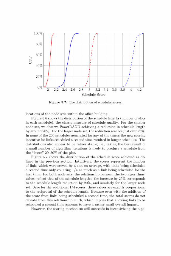
2 2.2 2.4 2.6 2.8 3 3.2 3.4 3.6 3.8 4 4.20%

20%

40%

60%

80%

100%

Schedule Score

CD

F

Figure 5.7: The distribution of schedules scores.

locations of the node sets within the office building.Figure 5.6 shows the distribution of the schedule lengths (number of slots

in each schedule), the classic measure of schedule quality. For the smallernode set, we observe PowerRAND achieving a reduction in schedule lengthby around 20%. For the larger node set, the reduction reaches just over 25%.In none of the 200 schedules generated for any of the traces the new scoringincentive for links scheduled a second time resulted in longer schedules. Thedistributions also appear to be rather stable, i.e., taking the best result ofa small number of algorithm iterations is likely to produce a schedule fromthe “lower” 20–30% of the plot.

Figure 5.7 shows the distribution of the schedule score achieved as de-fined in the previous section. Intuitively, the scores represent the numberof links which were served by a slot on average, with links being scheduleda second time only counting 1/4 as much as a link being scheduled for thefirst time. For both node sets, the relationship between the two algorithms’values reflect that of the schedule lengths: the increase by 25% correspondsto the schedule length reduction by 20%, and similarly for the larger nodeset. Save for the additional 1/4 scores, these values are exactly proportionalto the reciprocal of the schedule length. Because even with the addition ofthe score from links being scheduled a second time, the total scores do notdeviate from this relationship much, which implies that allowing links to bescheduled a second time appears to have a rather small overall impact.

However, the scoring mechanism still succeeds in incentivizing the algo-

1.8 2 2.2 2.4 2.6 2.8 3 3.2 3.4 3.6 3.8 40%

20%

40%

60%

80%

100%

Average Links per Slot

CD

F

Figure 5.8: The distribution of the average links per slot for RAND without (thintraces) and with (thick traces) the new scoring.

2 2.5 3 3.5 4 4.5 50%

20%

40%

60%

80%

100%

Average Links per Slot

CD

F

Figure 5.9: The distribution of the average links per slot for PowerRAND without(thin traces) and with (thick traces) the new scoring.

10 12 14 16 18 20 22 240%

20%

40%

60%

80%

100%

Predicted Slot SINR

CD

F

Figure 5.10: The distribution of the SINR values. The thinner traces show thevalues before slot optimization, the thicker traces the values after.

rithms to fill their slots up: Figures 5.8 and 5.9 show the distributions ofthe average over the number of links in a slot. For comparison, the thinnertraces in this plot each show a separate set of 200 schedules (colors anddashes as before) that were computed without the new scoring incentive(but still use the same link and prediction models). Both algorithms appearto achieve a similar increase in links per slot, with the PowerRAND doingslightly better on the smaller node set. The larger node set profits more fromthis (35% versus 20–25% for the smaller set), which was to be expected dueto the larger flexibility stemming from an overall larger number of links andnodes.

Figure 5.10 demonstrates the improvement in SINR values that is achievedthrough the optimization of individual slots after completion of the sched-ule computation. This optimization does not apply to regular RAND as itassumes the use of power control. The thinner traces in this plot correspondto the values before the optimization, the thicker traces conversely to afterthe optimization. No link is scheduled with a SINR value lower than 9 dBas this was precisely the cutoff we configured for the prediction model. For20–40% of links the optimization appears to have little to no impact. Theselinks are mostly part of already tightly packed slots without room for poweradjustments. For the remaining links the improvement is on the order of1–2 dB on average. While not a lot, in turbulent environments, every littleadditional stability translates into fewer mispredictions and longer lasting

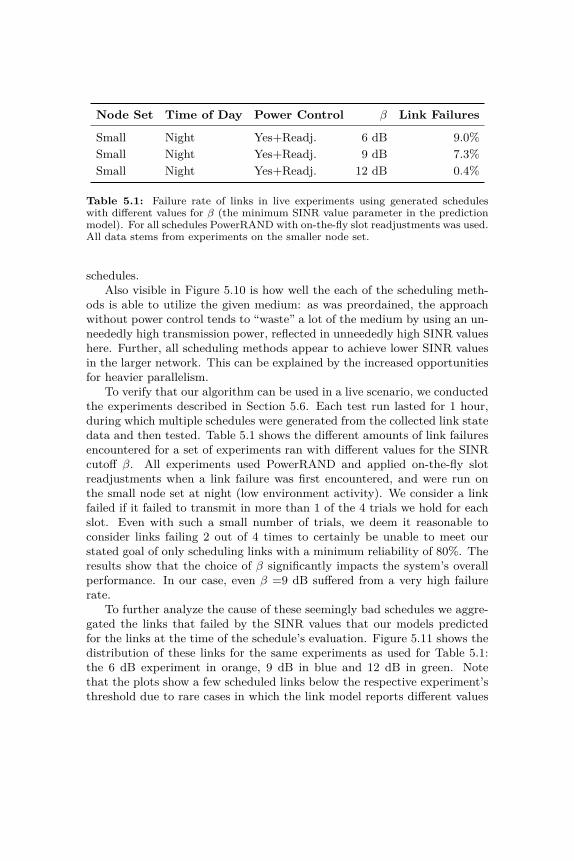
Node Set Time of Day Power Control β Link Failures

Small Night Yes+Readj. 6 dB 9.0%Small Night Yes+Readj. 9 dB 7.3%Small Night Yes+Readj. 12 dB 0.4%

Table 5.1: Failure rate of links in live experiments using generated scheduleswith different values for β (the minimum SINR value parameter in the predictionmodel). For all schedules PowerRAND with on-the-fly slot readjustments was used.All data stems from experiments on the smaller node set.

schedules.Also visible in Figure 5.10 is how well the each of the scheduling meth-

ods is able to utilize the given medium: as was preordained, the approachwithout power control tends to “waste” a lot of the medium by using an un-neededly high transmission power, reflected in unneededly high SINR valueshere. Further, all scheduling methods appear to achieve lower SINR valuesin the larger network. This can be explained by the increased opportunitiesfor heavier parallelism.

To verify that our algorithm can be used in a live scenario, we conductedthe experiments described in Section 5.6. Each test run lasted for 1 hour,during which multiple schedules were generated from the collected link statedata and then tested. Table 5.1 shows the different amounts of link failuresencountered for a set of experiments ran with different values for the SINRcutoff β. All experiments used PowerRAND and applied on-the-fly slotreadjustments when a link failure was first encountered, and were run onthe small node set at night (low environment activity). We consider a linkfailed if it failed to transmit in more than 1 of the 4 trials we hold for eachslot. Even with such a small number of trials, we deem it reasonable toconsider links failing 2 out of 4 times to certainly be unable to meet ourstated goal of only scheduling links with a minimum reliability of 80%. Theresults show that the choice of β significantly impacts the system’s overallperformance. In our case, even β =9 dB suffered from a very high failurerate.

To further analyze the cause of these seemingly bad schedules we aggre-gated the links that failed by the SINR values that our models predictedfor the links at the time of the schedule’s evaluation. Figure 5.11 shows thedistribution of these links for the same experiments as used for Table 5.1:the 6 dB experiment in orange, 9 dB in blue and 12 dB in green. Notethat the plots show a few scheduled links below the respective experiment’sthreshold due to rare cases in which the link model reports different values

0 2 4 6 8 10 12 14 160%

20%

40%

60%

80%

100%

Predicted Slot SINR

CD

F

6 dB9 dB12 dB

Figure 5.11: Distribution of the predicted SINR values of the links that failed inthe experiments listed in Table 5.1.

at the time of schedule generation and at the time of schedule evaluation(which lie a few seconds apart). Save for these exceptions, most of the linkfailures occur in the range of 9–11 dB. For the case of β = 9 dB this is notvery surprising, as we’d expect the weakest links in a schedule to fail themost frequently. However, we are unsure why most links failed around 9 dBin the case of β = 6 dB. In the 12 dB experiment only 3 links failed, allwell above the 9 dB mark. In conclusion, we find that even at night, whenthe environment should fluctuate only very little, links with predicted SINRvalues of 9 dB, in some rare cases even as high as 16 dB, may fail.

In another set of experiments we compared the link failures incurred byRAND to those by PowerRAND. Additionally, we distinguish PowerRANDwith and without the technique of on-the-fly slot readjustments (see Sec-tion 5.5). This technique does not apply to RAND as it requires powercontrol. Again, all experiments were run at night and on the smaller nodeset. The results are shown in Table 5.2.

Interestingly, at night, RAND suffers fewer failures than vanilla Power-RAND. This is likely due to the inherent overprovisioning of transmissionpower in RAND, and, conversely, due to PowerRAND cutting more corners.Once we allow PowerRAND to adapt transmission powers within a slot toreact to failing links, in the experiments ran at night, PowerRAND’s linkfailure rate falls to only 0.2% (0.4% in the test run with identical parametersshown in Table 5.1). During daytime, both RAND and PowerRAND suf-

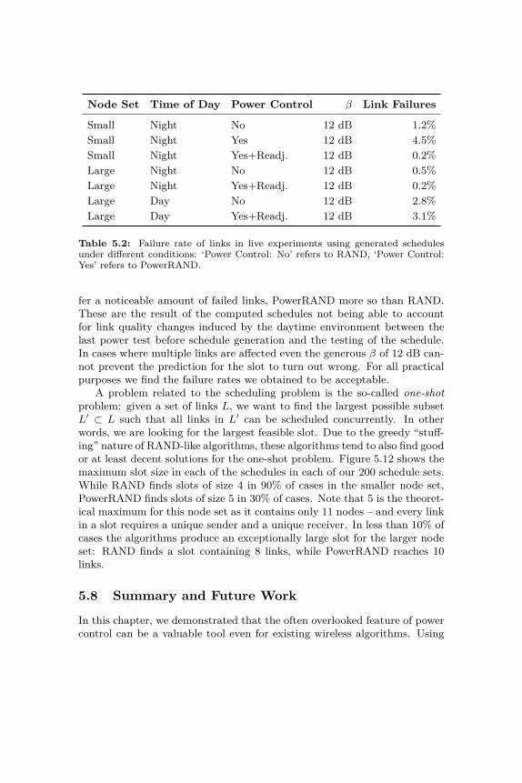
Node Set Time of Day Power Control β Link Failures

Small Night No 12 dB 1.2%Small Night Yes 12 dB 4.5%Small Night Yes+Readj. 12 dB 0.2%Large Night No 12 dB 0.5%Large Night Yes+Readj. 12 dB 0.2%Large Day No 12 dB 2.8%Large Day Yes+Readj. 12 dB 3.1%

Table 5.2: Failure rate of links in live experiments using generated schedulesunder different conditions: ‘Power Control: No’ refers to RAND, ‘Power Control:Yes’ refers to PowerRAND.

fer a noticeable amount of failed links, PowerRAND more so than RAND.These are the result of the computed schedules not being able to accountfor link quality changes induced by the daytime environment between thelast power test before schedule generation and the testing of the schedule.In cases where multiple links are affected even the generous β of 12 dB can-not prevent the prediction for the slot to turn out wrong. For all practicalpurposes we find the failure rates we obtained to be acceptable.

A problem related to the scheduling problem is the so-called one-shotproblem: given a set of links L, we want to find the largest possible subsetL′ ⊂ L such that all links in L′ can be scheduled concurrently. In otherwords, we are looking for the largest feasible slot. Due to the greedy “stuff-ing” nature of RAND-like algorithms, these algorithms tend to also find goodor at least decent solutions for the one-shot problem. Figure 5.12 shows themaximum slot size in each of the schedules in each of our 200 schedule sets.While RAND finds slots of size 4 in 90% of cases in the smaller node set,PowerRAND finds slots of size 5 in 30% of cases. Note that 5 is the theoret-ical maximum for this node set as it contains only 11 nodes – and every linkin a slot requires a unique sender and a unique receiver. In less than 10% ofcases the algorithms produce an exceptionally large slot for the larger nodeset: RAND finds a slot containing 8 links, while PowerRAND reaches 10links.


In this chapter, we demonstrated that the often overlooked feature of powercontrol can be a valuable tool even for existing wireless algorithms. Using

2 3 4 5 6 7 8 9 100%

20%

40%

60%

80%

100%

Maximum Links per Slot

CD

F

Figure 5.12: The distribution of the largest slot in the schedule.

the example of the simple yet powerful RAND scheduling algorithm, weshow that by augmenting the algorithm to fine-tune transmission powers,we can improve the produced schedules as measured by various metrics. Ourmain result is the reduction in the length of the produced schedules by 20–25% as shown in Figure 5.6. Additionally, we propose other improvementspossible with power control, such as optimization of SINR values within aslot and the on-the-fly adjustment to smaller changes in the environment.We verified that the shorter schedules our proposed PowerRAND algorithmproduces are also feasible in practice.

One goal for future work is the integration of PowerRAND into a fully-fledged MAC layer implementation. The main issue to be addressed here isthe overhead we incurred in our setup in the name of measurement accu-racy. We perform power test phases every 2 minutes, which reserve slots foreach node to transmit a packet alone, such that all other nodes are able torecord the results without interference. While in practice lowering the testfrequency to only once every 10 minutes, or testing only before computinga new schedule, is likely to suffice, such test phases still impose a significantoverhead to regular operations.

The most ambitious solution we are envisioning is to adapt the link modelnot based on dedicated power tests, but purely on feedback from regularnetwork operation: e.g., which links in which slots failed and succeeded,what accumulated power levels every node measures during every slot – evenif the node does not participate in any transmissions in that slot. Further,

changes to one link often also affect many others – perhaps all other linkssharing a certain node or passing through the same hallway. Examples forsuch behavior are easy to find. One instance can be seen between power tests#11 and #12 in Figure 5.3. Harnessing the implicitly available informationabout such changes may be the key to avoiding regular sweeping power tests.

The other issue to address is the centralized nature of our setup. For aMAC layer to be practical, all its components should be distributed amongstthe nodes of the network itself. As described earlier, it is not possible forPowerRAND to follow the same route from RAND to DRAND to achievedistributedness, mainly due to DRAND’s simplified model of the network.However, we are confident that PowerRAND can be transferred to dis-tributed operation by making some reasonable tradeoffs.

It may also be worthwhile to explore different avenues for dealing withunreliable links and slots. In this chapter, we focused on delivering a proofof concept for the possible benefits of power control, which is made clearerby avoiding, for instance, links that only successfully transmit in half of allattempts on average. If we are able to determine the rough probabilitiesfor a successful transmission of a link, we may be able to simply scheduleit multiple times to reach a desired average throughput. Alternatively, wecould catch up on failed links every couple of executions of the schedule.Even more ambitiously, the schedule could constantly be adapted as linksand traffic demands change. We already implemented a basic version of thiswith our slot readjustment technique responding to links underperforming.

6Conclusion

In spite of the rapid spread of wireless technology, the space of both feasiblewireless transmission primitives as well as algorithms making use of thoseprimitives has yet to be fully explored. In this work, we made a contributionto this space by filling in a few of the many blanks. We investigated multipleapplications that suffer when treated under traditional wired network basedabstractions, and designed and evaluated solutions tailored to the wirelessmedium.

We showed that the combination of transmission power control and thecapture effect may allow for traffic prioritization completely without over-head. Critical to the success of this method are the homogeneity of thenetwork, or, more specifically, how small the biggest difference in “length”between any two links at a single node is, and the flexibility of the wirelessnodes in terms of transmission power values available. Using TelosB moteson the FlockLab testbed we found the network to generally support at least2 priority layers at every node. Our distributed fire alarm implementationindeed proved apt at quickly reporting high-priority alarms while causinglittle to no overhead to the low-priority protocol.

We showed the feasibility of synchronizing run-of-the-mill wireless sensornodes’ clocks well enough to achieve constructive interference. Unlike pre-vious work, our solution does not require each sender to receive a common

107

reference packet. Instead, it focuses on minimizing the error sources of clocksynchronization and transmission timing.

Breaking with the abstraction that every packet is sent and received as asingle packet, we considered possible applications for mixed sender schemesand explored the practical difficulties that needed to be overcome. Usingsignals of different strengths or by prematurely turning off a transmitter,receivers can be fooled into decoding a packet with mismatching synchro-nization headers and payloads. If we don’t get lucky and the symbol stringphases are not approximately the same, we are sometimes still able to puzzlethe payload back together by exploiting certain relationships between thesymbols’ chip sequences.

Finally, we examined how power control can be applied to the RANDscheduling algorithm. We developed a power control aware version calledPowerRAND, which attempts to use each link at the minimum possible op-erating power to minimize interference, and then in a second step optimizesthe link powers within each slot. PowerRAND achieves schedules 20–25%shorter than RAND, and our proof of concept implementation showed thatthey are generally just as reliable in practice. Additionally, we investigatedhow power control allows schedules to react to changes in the environment.

While our protocol layering solution is already directly applicable topractice, the other results mostly remained as proofs of concept. Integratingthese techniques into general purpose frameworks is left to future work. Formany of these approaches, it would also be interesting to apply them to morepowerful hardware: they are all limited in one way or another either by theavailable clock precision or by the granularity of the set of programmabletransmission powers. Perhaps future hardware may also cater better tothese needs.

Ultimately, the grand goal of our work is to inspire other applicationsto make more use of the wireless medium’s unique properties. As virtuallyall sensor network MAC layers ignore power control, we envision that anyMAC layer protocol X may be enriched to become PowerX, improving theprotocol’s characteristics such as medium utilization and throughput. Ourtreatment of RAND did not rely on any properties specific to RAND, yetPowerRAND certainly improved significantly over RAND. We do not seeany reason why such an effect should not be repeatable across more wirelessalgorithms.

Bibliography

[1] Ash, D.L.: A comparison between OOK/ASK and FSK modulationtechniques for radio links. Technical report, Technical report, RF Mono-lithics Inc (1992)

[2] Brar, G.S., Blough, D.M., Santi, P.: Computationally efficient schedul-ing with the physical interference model for throughput improvementin wireless mesh networks. In: Proceedings of the 12th Annual Interna-tional Conference on Mobile Computing and Networking (MobiCom).(2006) 2–13

[3] Burri, N., von Rickenbach, P., Wattenhofer, R.: Dozer: ultra-lowpower data gathering in sensor networks. In: Proceedings of the 6th

International Conference on Information Processing in Sensor Networks(IPSN). (2007) 450–459

[4] Chafekar, D., Kumar, V.S.A., Marathe, M.V., Parthasarathy, S., Srini-vasan, A.: Cross-layer latency minimization in wireless networks withSINR constraints. In: Proceedings of the 8th ACM Interational Sympo-sium on Mobile Ad Hoc Networking and Computing (MobiHoc). (2007)110–119

[5] Chafekar, D., Kumar, V.S.A., Marathe, M.V., Parthasarathy, S., Srini-vasan, A.: Approximation algorithms for computing capacity of wire-less networks with SINR constraints. In: 27th IEEE International Con-ference on Computer Communications (INFOCOM). (2008) 1166–1174

[6] Chang, H., Misra, V., Rubenstein, D.: A general model and analysis ofphysical layer capture in 802.11 networks. In: 25th IEEE InternationalConference on Computer Communications (INFOCOM). (2006)

109

[7] Chen, Y., Terzis, A.: On the mechanisms and effects of calibratingRSSI measurements for 802.15.4 radios. In: Wireless Sensor Networks,7th European Conference (EWSN). Volume 5970 of Lecture Notes inComputer Science. (2010) 256–271

[8] Cidon, A., Nagaraj, K., Katti, S., Viswanath, P.: Flashback: decoupledlightweight wireless control. In: ACM SIGCOMM Computer Commu-nication Review. Volume 42. (2012) 223–234

[9] Davis, D.H., Gronemeyer, S.: Performance of slotted ALOHA ran-dom access with delay capture and randomized time of arrival. IEEETransactions on Communications 28(5) (1980) 703–710

[10] Dinitz, M.: Distributed algorithms for approximating wireless networkcapacity. In: 29th IEEE International Conference on Computer Com-munications (INFOCOM). (2010) 1397–1405

[11] Doddavenkatappa, M., Chan, M.C.: P 3: a practical packet pipelineusing synchronous transmissions for wireless sensor networks. In: Pro-ceedings of the 13th International Symposium on Information Process-ing in Sensor Networks (IPSN). (2014) 203–214

[12] Dunkels, A., Gronvall, B., Voigt, T.: Contiki - A lightweight andflexible operating system for tiny networked sensors. In: 29th AnnualIEEE Conference on Local Computer Networks (LCN). (2004) 455–462

[13] Dutta, P., Musaloiu-Elefteri, R., Stoica, I., Terzis, A.: Wireless ACKcollisions not considered harmful. In: 7th ACM Workshop on Hot Top-ics in Networks (HotNets). (2008) 19–24

[14] ElBatt, T.A., Ephremides, A.: Joint scheduling and power control forwireless ad hoc networks. IEEE Transactions on Wireless Communica-tions 3(1) (2004) 74–85

[15] Elson, J., Girod, L., Estrin, D.: Fine-grained network time synchro-nization using reference broadcasts. In: 5th Symposium on OperatingSystem Design and Implementation (OSDI). (2002)

[16] Elson, J., Romer, K.: Wireless sensor networks: a new regime fortime synchronization. Computer Communication Review 33(1) (2003)149–154

[17] Fanghanel, A., Kesselheim, T., Racke, H., Vocking, B.: Oblivious inter-ference scheduling. In: Proceedings of the 28th Annual ACM Sympo-sium on Principles of Distributed Computing (PODC). (2009) 220–229

[18] Ferrari, F., Zimmerling, M., Mottola, L., Thiele, L.: Low-power wire-less bus. In: Proceedings of the 10th ACM Conference on EmbeddedNetwork Sensor Systems (SenSys). (2012) 1–14

[19] Ferrari, F., Zimmerling, M., Thiele, L., Saukh, O.: Efficient networkflooding and time synchronization with Glossy. In: Proceedings ofthe 10th International Conference on Information Processing in SensorNetworks (IPSN). (2011) 73–84

[20] Flury, R., Wattenhofer, R.: Slotted programming for sensor networks.In: Proceedings of the 9th International Conference on InformationProcessing in Sensor Networks (IPSN). (2010) 24–34

[21] Ganeriwal, S., Kumar, R., Srivastava, M.B.: Timing-sync protocol forsensor networks. In: Proceedings of the 1st International Conferenceon Embedded Networked Sensor Systems (SenSys). (2003) 138–149

[22] Ghosh, A., Ratasuk, R., Xiao, W., Classon, B.K., Nangia, V., Love,R., Schwent, D., Wilson, D.: Uplink control channel design for 3GPPLTE. In: Proceedings of the IEEE 18th International Symposium onPersonal, Indoor and Mobile Radio Communications (PIMRC). (2007)1–5

[23] Gotzhein, R., Kuhn, T.: Black burst synchronization (BBS) - A proto-col for deterministic tick and time synchronization in wireless networks.Computer Networks 55(13) (2011) 3015–3031

[24] Goussevskaia, O., Oswald, Y.A., Wattenhofer, R.: Complexity in geo-metric SINR. In: Proceedings of the 8th ACM Interational Symposiumon Mobile Ad Hoc Networking and Computing (MobiHoc). (2007) 100–109

[25] Gronkvist, J., Hansson, A.: Comparison between graph-based andinterference-based STDMA scheduling. In: Proceedings of the 2nd ACMInterational Symposium on Mobile Ad Hoc Networking and Computing(MobiHoc). (2001) 255–258

[26] Gupta, P., Kumar, P.R.: The capacity of wireless networks. IEEETransactions on Information Theory 46(2) (2000) 388–404

[27] Halldorsson, M.M.: Wireless scheduling with power control. ACMTransactions on Algorithms 9(1) (2012) 7:1–7:20

[28] Halldorsson, M.M., Tonoyan, T.: The price of local power control inwireless scheduling. In: 35th IARCS Annual Conference on Foundationof Software Technology and Theoretical Computer Science (FSTTCS).Volume 45. (2015) 529–542

[29] Hanel, T., Krampe, F., Gericke, C., Aschenbruck, N.: On the po-tential of data-based time synchronization in wireless sensor networksfor condition monitoring. In: International Conference on DistributedComputing in Sensor Systems (DCOSS). (2016) 216–224

[30] Hasler, A., Gruber, S., Beutel, J.: Kinematics of steep bedrock per-mafrost. Journal of Geophysical Research: Earth Surface 117(F1)(2012)

[31] Huang, P., Desai, M., Qiu, X., Krishnamachari, B.: On the multihopperformance of synchronization mechanisms in high propagation delaynetworks. IEEE Transactions on Computers 58(5) (2009) 577–590

[32] Institute of Electrical and Electronics Engineers: IEEE Standard802.15.4: Wireless Medium Access Control (MAC) and Physical Layer(PHY) Specifications for Low-Rate Wireless Personal Area Networks

[33] Jayasuriya, A., Perreau, S., Dadej, A., Gordon, S.: Hidden vs exposedterminal problem in ad hoc networks. PhD thesis, ATNAC (2004)

[34] Johansson, N., Korner, U., Johansson, P.: Performance evaluation ofscheduling algorithms for Bluetooth. In: Broadband Communications:Convergence of Network Technologies, IFIP TC6 WG6.2 Fifth Interna-tional Conference on Broadband Communications (BC). Volume 159.(1999) 139–150

[35] Kesselheim, T.: A constant-factor approximation for wireless capacitymaximization with power control in the SINR model. In: Proceedingsof the Twenty-Second Annual ACM-SIAM Symposium on Discrete Al-gorithms (SODA). (2011) 1549–1559

[36] Kochut, A., Vasan, A., Shankar, A.U., Agrawala, A.K.: Sniffing outthe correct physical layer capture model in 802.11b. In: 12th IEEEInternational Conference on Network Protocols (ICNP). (2004) 252–261

[37] Kusy, B., Dutta, P., Levis, P., Maroti, M., Ledeczi, A., Culler, D.E.:Elapsed time on arrival: a simple and versatile primitive for canonicaltime synchronisation services. International Journal of Ad Hoc andUbiquitous Computing (IJAHUC) 1(4) (2006) 239–251

[38] Landsiedel, O., Ferrari, F., Zimmerling, M.: Chaos: versatile andefficient all-to-all data sharing and in-network processing at scale. In:Proceedings of the 11th ACM Conference on Embedded Network SensorSystems (SenSys). (2013) 1:1–1:14

[39] Lee, J., Kim, W., Lee, S., Jo, D., Ryu, J., Kwon, T., Choi, Y.: Anexperimental study on the capture effect in 802.11a networks. In: Pro-ceedings of the Second ACM Workshop on Wireless Network Testbeds,Experimental Evaluation and Characterization (WINTECH). (2007)19–26

[40] Leentvaar, K., Flint, J.H.: The capture effect in FM receivers. IEEETransactions on Communications 24(5) (1976) 531–539

[41] Lenzen, C., Sommer, P., Wattenhofer, R.: PulseSync: An efficient andscalable clock synchronization protocol. IEEE/ACM Transactions onNetworking (TON) 23(3) (2015) 717–727

[42] Li, B., Nie, L., Wu, C., Gonzalez, H., Lu, C.: Incorporating emer-gency alarms in reliable wireless process control. In: Proceedings of theACM/IEEE Sixth International Conference on Cyber-Physical Systems(ICCPS). (2015) 218–227

[43] Li, H., Feng, X., Shi, S., Zheng, F., Xie, X.: A high-accuracy clocksynchronization method in distributed real-time system. In: ComputerEngineering and Technology, 18th CCF Conference, NCCET 2014. Vol-ume 491 of Communications in Computer and Information Science.(2015) 148–157

[44] Li, X., Zeng, Q.A.: Performance analysis of the IEEE 802.11 MACprotocol over a WLAN with capture effect. Information and MediaTechnologies (1) (2006) 679–685

[45] Liang, C.M., Chen, K., Priyantha, N.B., Liu, J., Zhao, F.: RushNet:practical traffic prioritization for saturated wireless sensor networks.In: Proceedings of the 12th ACM Conference on Embedded NetworkSensor Systems (SenSys). (2014) 105–118

[46] Lim, R., Ferrari, F., Zimmerling, M., Walser, C., Sommer, P., Beu-tel, J.: FlockLab: a testbed for distributed, synchronized tracing andprofiling of wireless embedded systems. In: Proceedings of the 12th In-ternational Conference on Information Processing in Sensor Networks(IPSN). (2013) 153–166

[47] Lin, S., Zhang, J., Zhou, G., Gu, L., Stankovic, J.A., He, T.: ATPC:adaptive transmission power control for wireless sensor networks. In:Proceedings of the 4th International Conference on Embedded Net-worked Sensor Systems (SenSys). (2006) 223–236

[48] Litjens, R., Roijers, F., Van den Berg, J., Boucherie, R.J., Fleuren, M.:Performance analysis of wireless LANs: an integrated packet/flow levelapproach. Teletraffic Science and Engineering 5 (2003) 931–940

[49] Lu, J., Whitehouse, K.: Flash flooding: Exploiting the capture effectfor rapid flooding in wireless sensor networks. In: INFOCOM 2009. 28th

IEEE International Conference on Computer Communications. (2009)2491–2499

[50] Lynch, J.P., Loh, K.J.: A summary review of wireless sensors andsensor networks for structural health monitoring. Shock and VibrationDigest 38(2) (2006) 91–130

[51] Maheshwari, R., Jain, S., Das, S.R.: A measurement study of interfer-ence modeling and scheduling in low-power wireless networks. In: Pro-ceedings of the 6th International Conference on Embedded NetworkedSensor Systems (SenSys). (2008) 141–154

[52] Manweiler, J., Santhapuri, N., Sen, S., Choudhury, R.R., Nelakuditi,S., Munagala, K.: Order matters: Transmission reordering in wirelessnetworks. IEEE/ACM Transactions on Networking 20(2) (2012) 353–366

[53] Maroti, M., Kusy, B., Simon, G., Ledeczi, A.: The flooding time syn-chronization protocol. In: Proceedings of the 2nd International Confer-ence on Embedded Networked Sensor Systems (SenSys). (2004) 39–49

[54] Maroti, M., Kusy, B., Simon, G., Ledeczi, A.: Robust multi-hop timesynchronization in sensor networks. In: Proceedings of the Interna-tional Conference on Wireless Networks (ICWN). (2004) 454–460

[55] Mills, D.L.: Internet time synchronization: the network time protocol.IEEE Transactions on Communications 39(10) (1991) 1482–1493

[56] Moscibroda, T., Wattenhofer, R.: The complexity of connectivity inwireless networks. In: 25th IEEE International Conference on Com-puter Communications (INFOCOM). (2006)

[57] Moscibroda, T., Wattenhofer, R., Weber, Y.: Protocol design beyondgraph-based models. In: 5th ACM Workshop on Hot Topics in Networks(HotNets). (2006) 25–30

[58] Moscibroda, T., Wattenhofer, R., Zollinger, A.: Topology control meetsSINR: the scheduling complexity of arbitrary topologies. In: Proceed-ings of the 7th ACM Interational Symposium on Mobile Ad Hoc Net-working and Computing (MobiHoc). (2006) 310–321

[59] Newzoo: Newzoo’s global mobile market report, April 2017. Technicalreport, Newzoo (2017)

[60] Nyandoro, A., Libman, L., Hassan, M.: Service differentiation using thecapture effect in 802.11 wireless LANs. IEEE Transactions on WirelessCommunications 6(8) (2007) 2961–2971

[61] Patras, P., Qi, H., Malone, D.: Mitigating collisions through power-hopping to improve 802.11 performance. Pervasive and Mobile Com-puting 11 (2014) 41–55

[62] Polastre, J., Szewczyk, R., Culler, D.E.: Telos: enabling ultra-lowpower wireless research. In: Proceedings of the Fourth InternationalSymposium on Information Processing in Sensor Networks (IPSN).(2005) 364–369

[63] Ramanathan, S.: A unified framework and algorithm for channel as-signment in wireless networks. Wireless Networks 5(2) (1999) 81–94

[64] Ray, S., Carruthers, J.B., Starobinski, D.: RTS/CTS-induced conges-tion in ad hoc wireless LANs. In: 2003 IEEE Wireless Communicationsand Networking (WCNC). Volume 3. (2003) 1516–1521

[65] Rhee, I., Warrier, A., Aia, M., Min, J., Sichitiu, M.L.: Z-MAC: ahybrid MAC for wireless sensor networks. IEEE/ACM Transactions onNetworking (TON) 16(3) (2008) 511–524

[66] Rhee, I., Warrier, A., Min, J., Xu, L.: DRAND: distributed randomizedTDMA scheduling for wireless ad-hoc networks. In: Proceedings of the7th ACM Interational Symposium on Mobile Ad Hoc Networking andComputing (MobiHoc). (2006) 190–201

[67] Romer, K.: Time synchronization in ad hoc networks. In: Proceedingsof the 2nd ACM Interational Symposium on Mobile Ad Hoc Networkingand Computing (MobiHoc). (2001) 173–182

[68] Sallai, J., Kusy, B., Ledeczi, A., Dutta, P.: On the scalability of rout-ing integrated time synchronization. In: Wireless Sensor Networks,Third European Workshop (EWSN). Volume 3868 of Lecture Notes inComputer Science. (2006) 115–131

[69] Santhapuri, N.K., Manweiler, J., Sen, S., Choudhury, R.R., Nelakuditi,S., Munagala, K.: Message in message (MIM): A case for shufflingtransmissions in wireless networks. In: 7th ACM Workshop on HotTopics in Networks (HotNets). (2008) 25–30

[70] Schmid, T., Dutta, P., Srivastava, M.B.: High-resolution, low-powertime synchronization an oxymoron no more. In: Proceedings of the 9th

International Conference on Information Processing in Sensor Networks(IPSN). (2010) 151–161

[71] Selavo, L., Wood, A.D., Cao, Q., Sookoor, T.I., Liu, H., Srinivasan, A.,Wu, Y., Kang, W., Stankovic, J.A., Young, D., Porter, J.: LUSTER:wireless sensor network for environmental research. In: Proceedingsof the 5th International Conference on Embedded Networked SensorSystems (SenSys). (2007) 103–116

[72] Seth, A., Kroeker, D., Zaharia, M.A., Guo, S., Keshav, S.: Low-costcommunication for rural internet kiosks using mechanical backhaul. In:Proceedings of the 12th Annual International Conference on MobileComputing and Networking (MOBICOM). (2006) 334–345

[73] Son, D., Krishnamachari, B., Heidemann, J.S.: Experimental study ofconcurrent transmission in wireless sensor networks. In: Proceedingsof the 4th International Conference on Embedded Networked SensorSystems (SenSys). (2006) 237–250

[74] Su, L., Liu, C., Song, H., Cao, G.: Routing in intermittently connectedsensor networks. In: Proceedings of the 16th annual IEEE InternationalConference on Network Protocols (ICNP). (2008) 278–287

[75] Texas Instruments: 2.4 GHz IEEE 802.15.4 / ZigBee-ready RFTransceiver. CC2420 Data Sheet.

[76] Whitehouse, K., Woo, A., Jiang, F., Polastre, J., Culler, D.E.: Ex-ploiting the capture effect for collision detection and recovery. In: Pro-ceedings of the 2nd IEEE Workshop on Embedded Networked Sensors(EmNets). (2005) 45–52

[77] Xu, K., Gerla, M., Bae, S.: How effective is the IEEE 802.11 RT-S/CTS handshake in ad hoc networks. In: Proceedings of the GlobalTelecommunications Conference (GLOBECOM). (2002) 72–76

[78] Yuan, D., Hollick, M.: Let’s talk together: Understanding concur-rent transmission in wireless sensor networks. In: 38th Annual IEEEConference on Local Computer Networks (LCN). (2013) 219–227

[79] Yuan, D., Riecker, M., Hollick, M.: Making ‘Glossy’ networks sparkle:Exploiting concurrent transmissions for energy efficient, reliable, ultra-low latency communication in wireless control networks. In: WirelessSensor Networks, 11th European Conference (EWSN). Volume 8354 ofLecture Notes in Computer Science. (2014) 133–149

[80] Zimmerling, M., Ferrari, F., Mottola, L., Thiele, L.: On modelinglow-power wireless protocols based on synchronous packet transmis-sions. In: IEEE 21st International Symposium on Modelling, Analysisand Simulation of Computer and Telecommunication Systems (MAS-COTS). (2013) 546–555

[81] Zuniga, M., Krishnamachari, B.: Analyzing the transitional region inlow power wireless links. In: Proceedings of the First Annual IEEECommunications Society Conference on Sensor and Ad Hoc Communi-cations and Networks (SECON). (2004) 517–526

Publications

During my PhD studies at ETH Zurich, I co-authored the following publi-cations. The authors are listed in alphabetical order.

• On Local Fixing. Michael Konig and Roger Wattenhofer. 17th Inter-national Conference On Principles Of Distributed Systems (OPODIS),December 2013.

• Sharing a Medium Between Concurrent Protocols Without OverheadUsing the Capture Effect. Michael Konig and Roger Wattenhofer.13th International Conference on Embedded Wireless Systems and Net-works (EWSN), February 2016.

• Maintaining Constructive Interference Using Well-Synchronized Sen-sor Nodes. Michael Konig and Roger Wattenhofer. 12th Annual In-ternational Conference on Distributed Computing in Sensor Systems(DCOSS), May 2016.

• A Concept for an Introduction to Parallelization in Java: Multithread-ing with Programmable Robots in Minecraft. Klaus-Tycho Forster,Michael Konig and Roger Wattenhofer. 17th Annual Conference onInformation Technology Education (SIGITE), September 2016.

• Effectively Capturing Attention Using the Capture Effect. MichaelKonig and Roger Wattenhofer. 14th ACM Conference on EmbeddedNetworked Sensor Systems (SenSys), November 2016.

• Multi-Agent Pathfinding with n Agents on Graphs with n Vertices:Combinatorial Classification and Tight Algorithmic Bounds. Klaus-Tycho Forster, Linus Groner, Torsten Hoefler, Michael Konig, Sascha

Schmid and Roger Wattenhofer. 10th International Conference onAlgorithms and Complexity (CIAC), May 2017.

• Tempering Wireless Schedules. Michael Konig and Roger Watten-hofer. To appear.

adding more phy to the mac: exploiting physical … · adding more phy to the mac: ... 3.3...

Documents