Additive-Belief-Based Preferences∗

David Dillenberger† Collin Raymond‡

January 2018

Abstract

We introduce a new class of preferences — which we call additive-belief-based (ABB) util-

ity — that captures a general, but still tractable, approach to belief-based utility, and that

encompasses many popular models in the behavioral literature. We axiomatize a general class

of ABB preferences, as well as two prominent special cases that allow utility to depend on the

level of each period’s beliefs but not on changes in beliefs across periods. We also identify the

intersection of ABB preferences with the class of recursive preferences and characterize attitudes

towards the timing of resolution of uncertainty for such preferences.

JEL codes: D80, D81

Key words: Anticipatory utility, Compound lotteries, Preferences over beliefs, Recursive

preferences, Resolution of uncertainty.

1 Motivation

It is both intuitive and well documented that beliefs about future consumption or life events are

likely to directly affect well-being. For example, an individual may enjoy looking forward to an

upcoming vacation and particularly so if the risk of severe weather conditions became very unlikely;

on the other hand, the same individual may worry about a future medical procedure he determined

to undertake. Loewenstein (1987) used a survey technique to demonstrate the effect of anticipation

motives. There is also evidence based on fMRI studies that experience and anticipation of pain

produce psychological-stress reactions (Berns et. al., 2006; Lazarus, 1966).

Consequently, models of decision-making in which individuals derive utility not only from mate-

rial outcomes but also from their current and future beliefs have become increasingly prominent in

economics (see, for example, Caplin and Leahy, 2001; Koszegi and Rabin, 2009; and Ely, Frankel,

∗Acknowledgments: to be added†Department of Economics, University of Pennsylvania (ddill@sas.upenn.edu)‡Department of Economics, Purdue University (collinbraymond@gmail.com)

1

and Kamenica, 2015). In most of these models, overall utility is additively separable between ma-

terial payoffs and beliefs. Our aim in this paper is to introduce and analyze a new class of utility

functions — which we call additive-belief-based (ABB) utility — that captures a general additively

separable approach to belief-based utility.

Models within this class usually take one of two forms. The first, as in Caplin and Leahy (2001),

allows individuals’ utility to depend on the (absolute) level of beliefs; i.e., on how likely it is that

certain states/payoffs occur. In line with previous literature, we refer to these set of models as

anticipatory utility models. In the second, as in Koszegi and Rabin (2009), utility depends not on

the level of beliefs, but on changes in beliefs in any given period. We refer to this class as changing

beliefs models. Our ABB representation encompasses both these frameworks. Moreover, we point

out a useful partition of the class of anticipatory utility models into (i) prior-anticipatory utility

models, where utility depends on beliefs at the beginning of the time period, before information

has been received; and (ii) posterior-anticipatory utility models, where utility depends on beliefs at

the end of the time period, after information has been received.

While individuals in these models gain utility from their beliefs, they cannot directly choose

them. Rather, individuals begin with a prior belief, receive information, and form interim beliefs

by applying Bayes’ rule. Therefore, individuals can control their beliefs only by choosing particular

information structures. And since individuals gain utility from their beliefs, they may exhibit

preferences over information structures even if they cannot react to new information by altering

their behavior, that is, even if they do not have actions to take in the interim stage. This feature

is the one that distinguishes these models from the standard model, in which individuals would be

indifferent between all possible information structures when no actions are available. To tightly link

these models to observable behavior, we look at preferences over the combination of information

structures and prior beliefs. These can be elicited in a natural way in experimental and field

settings. Formally, taking advantage of the natural mapping between information structures and

compound lotteries, we take as our domain of preferences the set of two-stage compound lotteries,

that is, lotteries whose prizes are different lotteries over final outcomes.

In order to provide some intuition regarding the class of ABB functions, let P be a typical

two-stage compound lottery. In period 0 it induces a prior belief φ(P ); the individual knows that

the overall probability to receive xj in period 2 is φ(P )(xj). In period 1, P generates a signal i with

probability P (pi). Signal i generates a posterior belief over outcomes; the individual now knows

that in period 2 they will receive xj with probability pi(xj). In period 2, all uncertainty resolves

and the individual receives xj and has degenerate beliefs centering on this outcome (denoted δxj ).

The total utility of this scenario, denoted VABB(P ), is given by:

2

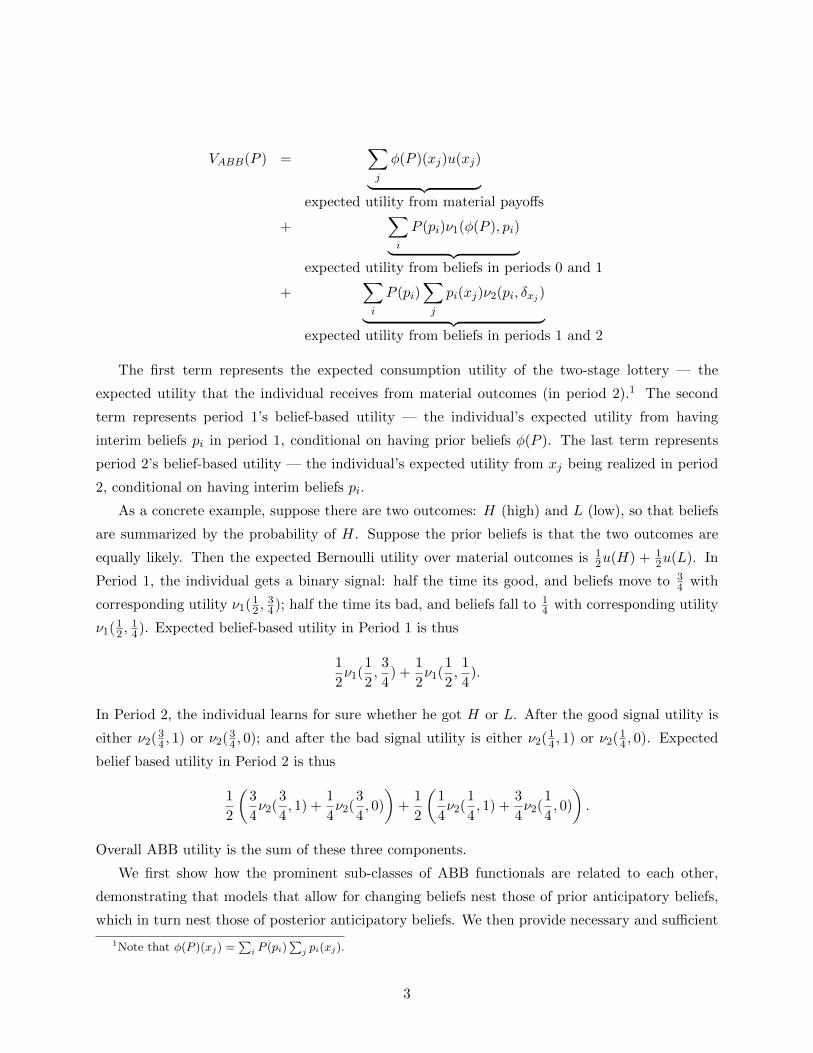
VABB(P ) =∑j

φ(P )(xj)u(xj)︸ ︷︷ ︸expected utility from material payoffs

+∑i

P (pi)ν1(φ(P ), pi)︸ ︷︷ ︸expected utility from beliefs in periods 0 and 1

+∑i

P (pi)∑j

pi(xj)ν2(pi, δxj )︸ ︷︷ ︸expected utility from beliefs in periods 1 and 2

The first term represents the expected consumption utility of the two-stage lottery — the

expected utility that the individual receives from material outcomes (in period 2).1 The second

term represents period 1’s belief-based utility — the individual’s expected utility from having

interim beliefs pi in period 1, conditional on having prior beliefs φ(P ). The last term represents

period 2’s belief-based utility — the individual’s expected utility from xj being realized in period

2, conditional on having interim beliefs pi.

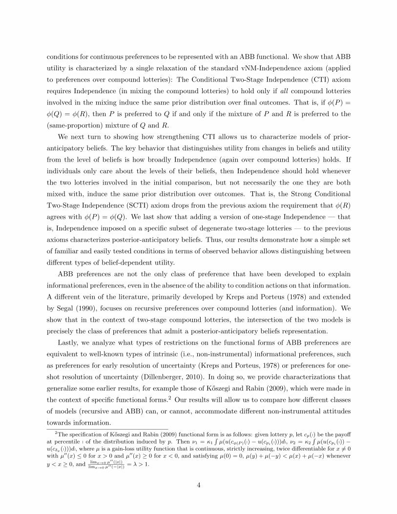
As a concrete example, suppose there are two outcomes: H (high) and L (low), so that beliefs

are summarized by the probability of H. Suppose the prior beliefs is that the two outcomes are

equally likely. Then the expected Bernoulli utility over material outcomes is 12u(H) + 1

2u(L). In

Period 1, the individual gets a binary signal: half the time its good, and beliefs move to 34 with

corresponding utility ν1(12 ,

34); half the time its bad, and beliefs fall to 1

4 with corresponding utility

ν1(12 ,

14). Expected belief-based utility in Period 1 is thus

1

2ν1(

1

2,3

4) +

1

2ν1(

1

2,1

4).

In Period 2, the individual learns for sure whether he got H or L. After the good signal utility is

either ν2(34 , 1) or ν2(3

4 , 0); and after the bad signal utility is either ν2(14 , 1) or ν2(1

4 , 0). Expected

belief based utility in Period 2 is thus

1

2

(3

4ν2(

3

4, 1) +

1

4ν2(

3

4, 0)

)+

1

2

(1

4ν2(

1

4, 1) +

3

4ν2(

1

4, 0)

).

Overall ABB utility is the sum of these three components.

We first show how the prominent sub-classes of ABB functionals are related to each other,

demonstrating that models that allow for changing beliefs nest those of prior anticipatory beliefs,

which in turn nest those of posterior anticipatory beliefs. We then provide necessary and sufficient

1Note that φ(P )(xj) =∑i P (pi)

∑j pi(xj).

3

conditions for continuous preferences to be represented with an ABB functional. We show that ABB

utility is characterized by a single relaxation of the standard vNM-Independence axiom (applied

to preferences over compound lotteries): The Conditional Two-Stage Independence (CTI) axiom

requires Independence (in mixing the compound lotteries) to hold only if all compound lotteries

involved in the mixing induce the same prior distribution over final outcomes. That is, if φ(P ) =

φ(Q) = φ(R), then P is preferred to Q if and only if the mixture of P and R is preferred to the

(same-proportion) mixture of Q and R.

We next turn to showing how strengthening CTI allows us to characterize models of prior-

anticipatory beliefs. The key behavior that distinguishes utility from changes in beliefs and utility

from the level of beliefs is how broadly Independence (again over compound lotteries) holds. If

individuals only care about the levels of their beliefs, then Independence should hold whenever

the two lotteries involved in the initial comparison, but not necessarily the one they are both

mixed with, induce the same prior distribution over outcomes. That is, the Strong Conditional

Two-Stage Independence (SCTI) axiom drops from the previous axiom the requirement that φ(R)

agrees with φ(P ) = φ(Q). We last show that adding a version of one-stage Independence — that

is, Independence imposed on a specific subset of degenerate two-stage lotteries — to the previous

axioms characterizes posterior-anticipatory beliefs. Thus, our results demonstrate how a simple set

of familiar and easily tested conditions in terms of observed behavior allows distinguishing between

different types of belief-dependent utility.

ABB preferences are not the only class of preference that have been developed to explain

informational preferences, even in the absence of the ability to condition actions on that information.

A different vein of the literature, primarily developed by Kreps and Porteus (1978) and extended

by Segal (1990), focuses on recursive preferences over compound lotteries (and information). We

show that in the context of two-stage compound lotteries, the intersection of the two models is

precisely the class of preferences that admit a posterior-anticipatory beliefs representation.

Lastly, we analyze what types of restrictions on the functional forms of ABB preferences are

equivalent to well-known types of intrinsic (i.e., non-instrumental) informational preferences, such

as preferences for early resolution of uncertainty (Kreps and Porteus, 1978) or preferences for one-

shot resolution of uncertainty (Dillenberger, 2010). In doing so, we provide characterizations that

generalize some earlier results, for example those of Koszegi and Rabin (2009), which were made in

the context of specific functional forms.2 Our results will allow us to compare how different classes

of models (recursive and ABB) can, or cannot, accommodate different non-instrumental attitudes

towards information.

2The specification of Koszegi and Rabin (2009) functional form is as follows: given lottery p, let cp(p) be the payoffat percentile p of the distribution induced by p. Then ν1 = κ1

∫µ(u(cφ(P )(p) − u(cpi(p)))dp, ν2 = κ2

∫µ(u(cpi(p)) −

u(cδx(p)))dp, where µ is a gain-loss utility function that is continuous, strictly increasing, twice differentiable for x 6= 0with µ′′(x) ≤ 0 for x > 0 and µ′′(x) ≥ 0 for x < 0, and satisfying µ(0) = 0, µ(y) + µ(−y) < µ(x) + µ(−x) whenever

y < x ≥ 0, and limx→0 µ′′(|x|)

limx→0 µ′′(−|x|) = λ > 1.

4

2 Model, Characterization, and Special Cases

Preliminaries:

Consider a set of prizes X, which is assumed to be a closed subset of some metric space. A

simple lottery p on X is a probability distribution over X with a finite support. Let ∆(X) (or

simply ∆) be the set of all simple lotteries on X. For any lotteries p, q ∈ ∆ and α ∈ (0, 1), we

let αp + (1 − α)q be the lottery that yields prize x with probability αp(x) + (1 − α)q(x). Denote

by δx the degenerate lottery that yields x with probability 1 and let X = {δx : x ∈ X}; we will

often abuse notation and refer to δx simply as x. Similarly, denote by ∆(∆(X)) (or simply ∆2)

the set of simple lotteries over ∆, that is, compound lotteries. For P,Q ∈ ∆2 and α ∈ (0, 1),

denote by R = αP + (1− α)Q the lottery that yields simple (one-stage) lottery p with probability

αP (p)+(1−α)Q(p). Denote by Dp the degenerate, in the first stage, compound lottery that yields

p with certainty. We sometime write a lottery (over either ∆ or ∆2) explicitly as a list; for example,

P = (p1, P (p1); . . . ; pn;P (pn)), or ((pi, P (pi))ni=1, denotes the two-stage lottery that, for i = 1, ..., n,

yields pi with probability P (pi). Define a reduction operator φ : ∆2 → ∆ that maps compound

lotteries to reduced one-stage lotteries by φ(Q) =∑

p∈∆Q(p)p.3

Two special subsets of compound lotteries are (i) Γ = {Dp|p ∈ ∆}, the set of degenerate lotteries

in ∆2. Γ is the set of late resolving lotteries, where any P ∈ Γ captures a situation in which the

information structure reveals no information in period 1, so that the interim posterior and prior

beliefs coincide; and (ii) Λ = {Q ∈ ∆2|Q(p) > 0 ⇒ p ∈ X}, the set of compound lotteries whose

outcomes are degenerate in ∆. Λ is the set of early resolving lotteries, where any P ∈ Λ captures

a situation in which the information structure reveals all information in period 1, so that interim

posteriors after observing any signal have one element in their support.

Our primitive is a binary relation % over ∆2. We define the restriction of % to the subsets Γ

and Λ as %Γ and %Λ, respectively.4

Functional Forms:

We first formally define additive-belief-based utility.

Definition 1. An additive-belief-based (ABB) representation is a tuple (u, ν1, ν2) consisting of

continuous functions u : X → R, ν1 : ∆×∆→ R, and ν2 : ∆× X → R, such that VABB : ∆2 → Rdefined as

3Such compound lotteries are isomorphic to the set of prior beliefs over outcomes X, plus a potential informationstructure. We can simply associate an information structure with the set of posterior beliefs it induces — the set ofsecond-stage lotteries.

4Note that both Γ and Λ are isomorphic to ∆, and therefore %Γ and %Λ can be interpreted as the the individual’spreferences over simple lotteries in the appropriate period.

5

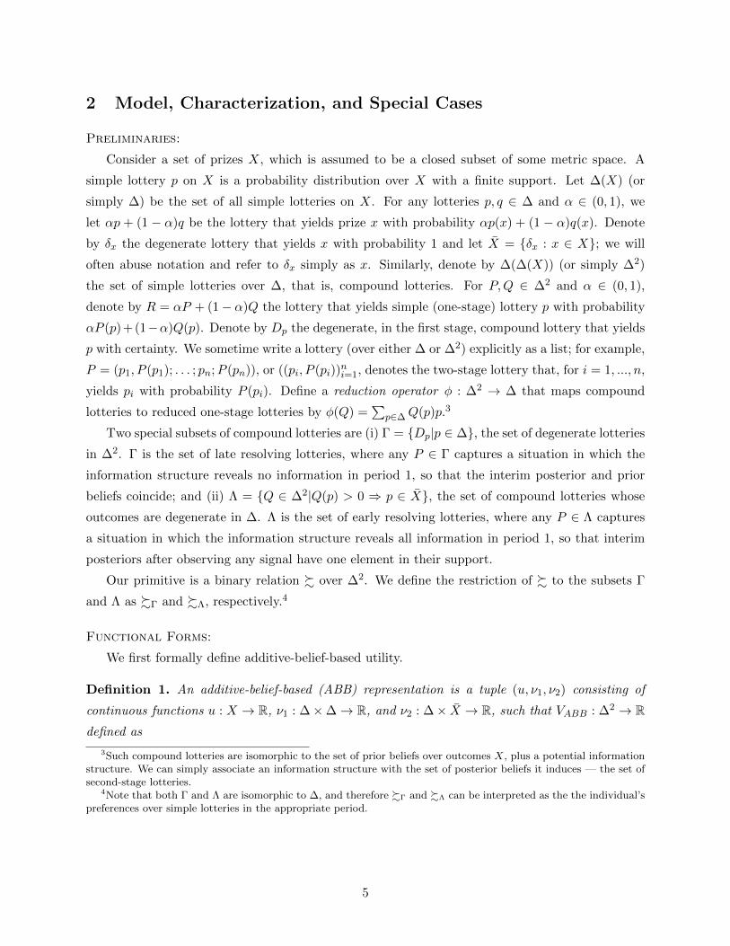
VABB(P ) =∑j

φ(P )(xj)u(xj) +∑i

P (pi)ν1(φ(P ), pi) +∑i

P (pi)∑j

pi(xj)ν2(pi, δxj )

represents %.

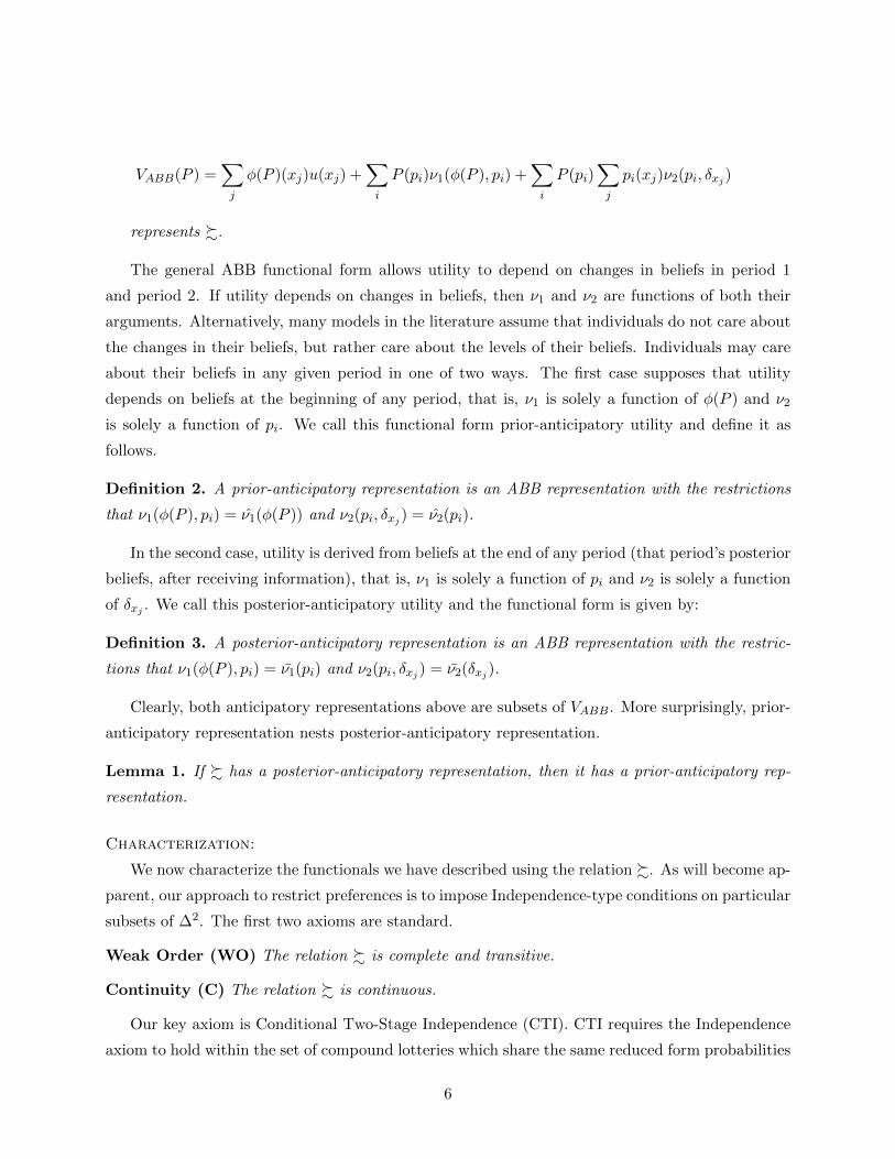
The general ABB functional form allows utility to depend on changes in beliefs in period 1

and period 2. If utility depends on changes in beliefs, then ν1 and ν2 are functions of both their

arguments. Alternatively, many models in the literature assume that individuals do not care about

the changes in their beliefs, but rather care about the levels of their beliefs. Individuals may care

about their beliefs in any given period in one of two ways. The first case supposes that utility

depends on beliefs at the beginning of any period, that is, ν1 is solely a function of φ(P ) and ν2

is solely a function of pi. We call this functional form prior-anticipatory utility and define it as

follows.

Definition 2. A prior-anticipatory representation is an ABB representation with the restrictions

that ν1(φ(P ), pi) = ν1(φ(P )) and ν2(pi, δxj ) = ν2(pi).

In the second case, utility is derived from beliefs at the end of any period (that period’s posterior

beliefs, after receiving information), that is, ν1 is solely a function of pi and ν2 is solely a function

of δxj . We call this posterior-anticipatory utility and the functional form is given by:

Definition 3. A posterior-anticipatory representation is an ABB representation with the restric-

tions that ν1(φ(P ), pi) = ν1(pi) and ν2(pi, δxj ) = ν2(δxj ).

Clearly, both anticipatory representations above are subsets of VABB. More surprisingly, prior-

anticipatory representation nests posterior-anticipatory representation.

Lemma 1. If % has a posterior-anticipatory representation, then it has a prior-anticipatory rep-

resentation.

Characterization:

We now characterize the functionals we have described using the relation %. As will become ap-

parent, our approach to restrict preferences is to impose Independence-type conditions on particular

subsets of ∆2. The first two axioms are standard.

Weak Order (WO) The relation % is complete and transitive.

Continuity (C) The relation % is continuous.

Our key axiom is Conditional Two-Stage Independence (CTI). CTI requires the Independence

axiom to hold within the set of compound lotteries which share the same reduced form probabilities

6

over outcomes (the same φ). Observe that the set {Q ∈ ∆2|φ(Q) = p} is convex for any p ∈ ∆.

Thus, CTI says that Independence holds along “slices” of the compound lottery space, where all

elements of the slice have the same reduced form probabilities.

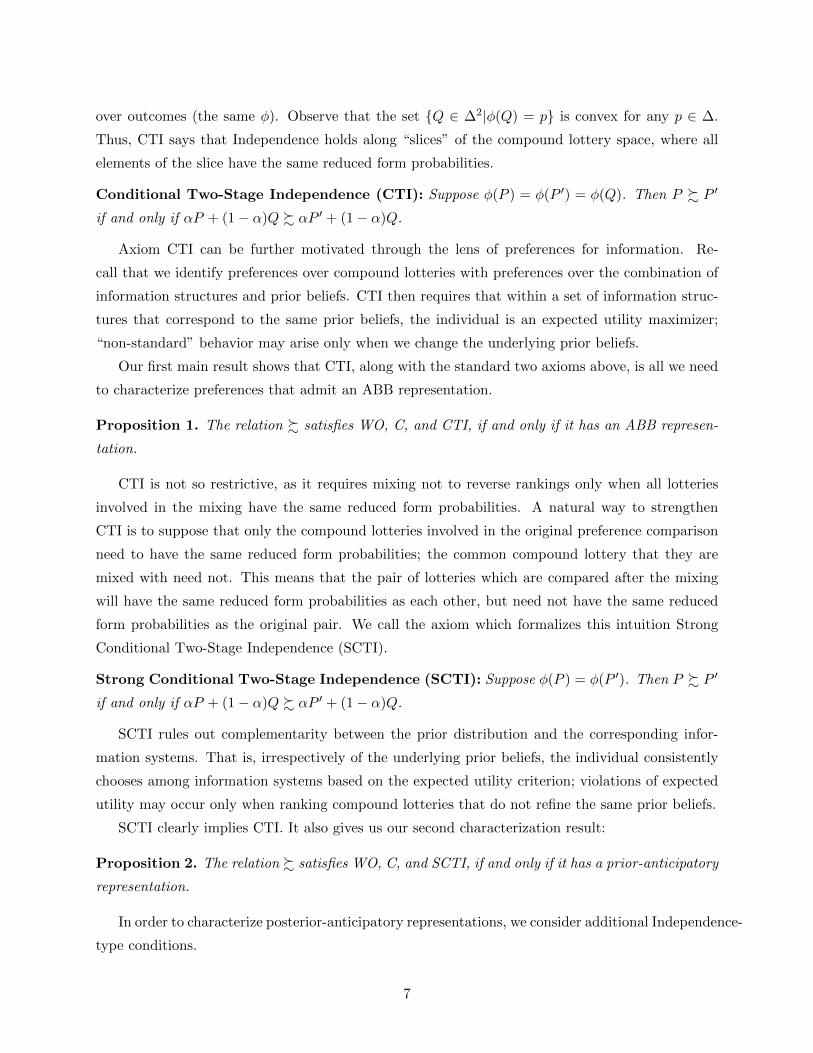
Conditional Two-Stage Independence (CTI): Suppose φ(P ) = φ(P ′) = φ(Q). Then P % P ′

if and only if αP + (1− α)Q % αP ′ + (1− α)Q.

Axiom CTI can be further motivated through the lens of preferences for information. Re-

call that we identify preferences over compound lotteries with preferences over the combination of

information structures and prior beliefs. CTI then requires that within a set of information struc-

tures that correspond to the same prior beliefs, the individual is an expected utility maximizer;

“non-standard” behavior may arise only when we change the underlying prior beliefs.

Our first main result shows that CTI, along with the standard two axioms above, is all we need

to characterize preferences that admit an ABB representation.

Proposition 1. The relation % satisfies WO, C, and CTI, if and only if it has an ABB represen-

tation.

CTI is not so restrictive, as it requires mixing not to reverse rankings only when all lotteries

involved in the mixing have the same reduced form probabilities. A natural way to strengthen

CTI is to suppose that only the compound lotteries involved in the original preference comparison

need to have the same reduced form probabilities; the common compound lottery that they are

mixed with need not. This means that the pair of lotteries which are compared after the mixing

will have the same reduced form probabilities as each other, but need not have the same reduced

form probabilities as the original pair. We call the axiom which formalizes this intuition Strong

Conditional Two-Stage Independence (SCTI).

Strong Conditional Two-Stage Independence (SCTI): Suppose φ(P ) = φ(P ′). Then P % P ′

if and only if αP + (1− α)Q % αP ′ + (1− α)Q.

SCTI rules out complementarity between the prior distribution and the corresponding infor-

mation systems. That is, irrespectively of the underlying prior beliefs, the individual consistently

chooses among information systems based on the expected utility criterion; violations of expected

utility may occur only when ranking compound lotteries that do not refine the same prior beliefs.

SCTI clearly implies CTI. It also gives us our second characterization result:

Proposition 2. The relation % satisfies WO, C, and SCTI, if and only if it has a prior-anticipatory

representation.

In order to characterize posterior-anticipatory representations, we consider additional Independence-

type conditions.

7

The first condition is logically independent from both CTI and SCTI. Axiom IΛ imposes Inde-

pendence over the set of lotteries that fully resolve in the first stage, Λ. (Since the set of lotteries

which resolve fully in the first stage is isomorphic to the set of one-stage lotteries, Independence

has a natural interpretation on this sub-domain.)

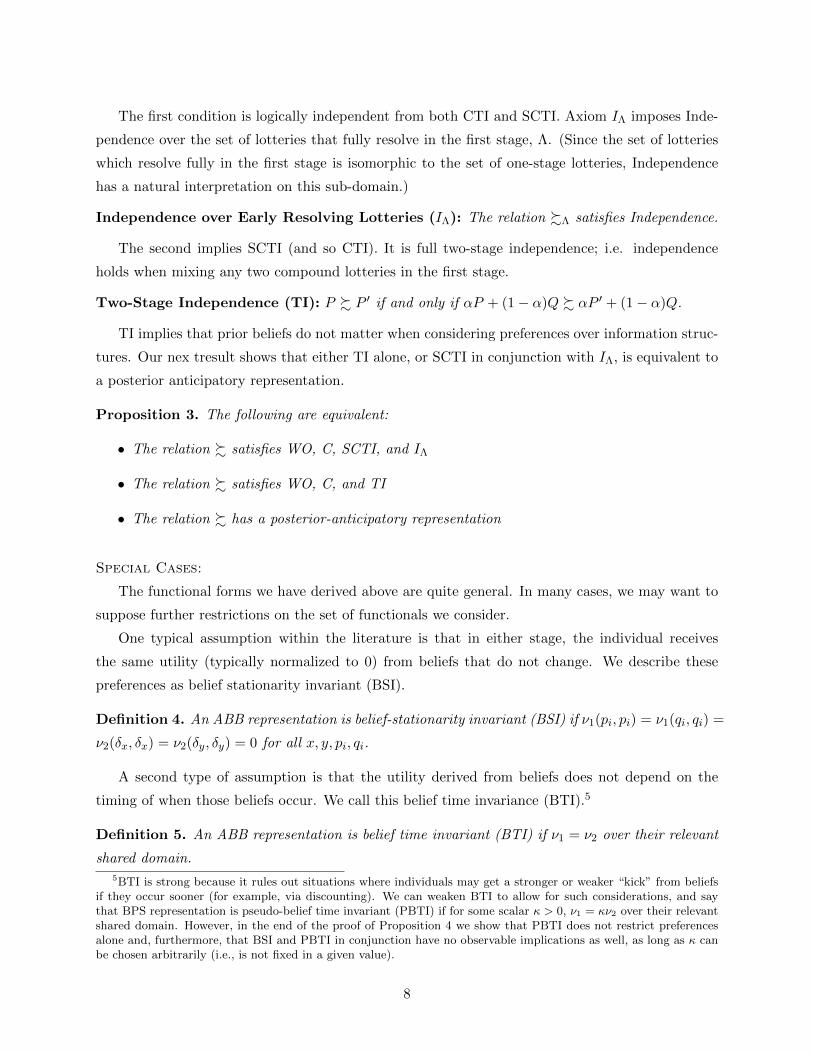
Independence over Early Resolving Lotteries (IΛ): The relation %Λ satisfies Independence.

The second implies SCTI (and so CTI). It is full two-stage independence; i.e. independence

holds when mixing any two compound lotteries in the first stage.

Two-Stage Independence (TI): P % P ′ if and only if αP + (1− α)Q % αP ′ + (1− α)Q.

TI implies that prior beliefs do not matter when considering preferences over information struc-

tures. Our nex tresult shows that either TI alone, or SCTI in conjunction with IΛ, is equivalent to

a posterior anticipatory representation.

Proposition 3. The following are equivalent:

• The relation % satisfies WO, C, SCTI, and IΛ

• The relation % satisfies WO, C, and TI

• The relation % has a posterior-anticipatory representation

Special Cases:

The functional forms we have derived above are quite general. In many cases, we may want to

suppose further restrictions on the set of functionals we consider.

One typical assumption within the literature is that in either stage, the individual receives

the same utility (typically normalized to 0) from beliefs that do not change. We describe these

preferences as belief stationarity invariant (BSI).

Definition 4. An ABB representation is belief-stationarity invariant (BSI) if ν1(pi, pi) = ν1(qi, qi) =

ν2(δx, δx) = ν2(δy, δy) = 0 for all x, y, pi, qi.

A second type of assumption is that the utility derived from beliefs does not depend on the

timing of when those beliefs occur. We call this belief time invariance (BTI).5

Definition 5. An ABB representation is belief time invariant (BTI) if ν1 = ν2 over their relevant

shared domain.5BTI is strong because it rules out situations where individuals may get a stronger or weaker “kick” from beliefs

if they occur sooner (for example, via discounting). We can weaken BTI to allow for such considerations, and saythat BPS representation is pseudo-belief time invariant (PBTI) if for some scalar κ > 0, ν1 = κν2 over their relevantshared domain. However, in the end of the proof of Proposition 4 we show that PBTI does not restrict preferencesalone and, furthermore, that BSI and PBTI in conjunction have no observable implications as well, as long as κ canbe chosen arbitrarily (i.e., is not fixed in a given value).

8

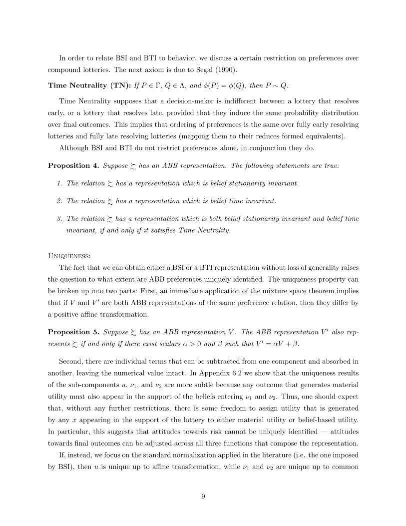
In order to relate BSI and BTI to behavior, we discuss a certain restriction on preferences over

compound lotteries. The next axiom is due to Segal (1990).

Time Neutrality (TN): If P ∈ Γ, Q ∈ Λ, and φ(P ) = φ(Q), then P ∼ Q.

Time Neutrality supposes that a decision-maker is indifferent between a lottery that resolves

early, or a lottery that resolves late, provided that they induce the same probability distribution

over final outcomes. This implies that ordering of preferences is the same over fully early resolving

lotteries and fully late resolving lotteries (mapping them to their reduces formed equivalents).

Although BSI and BTI do not restrict preferences alone, in conjunction they do.

Proposition 4. Suppose % has an ABB representation. The following statements are true:

1. The relation % has a representation which is belief stationarity invariant.

2. The relation % has a representation which is belief time invariant.

3. The relation % has a representation which is both belief stationarity invariant and belief time

invariant, if and only if it satisfies Time Neutrality.

Uniqueness:

The fact that we can obtain either a BSI or a BTI representation without loss of generality raises

the question to what extent are ABB preferences uniquely identified. The uniqueness property can

be broken up into two parts: First, an immediate application of the mixture space theorem implies

that if V and V ′ are both ABB representations of the same preference relation, then they differ by

a positive affine transformation.

Proposition 5. Suppose % has an ABB representation V . The ABB representation V ′ also rep-

resents % if and only if there exist scalars α > 0 and β such that V ′ = αV + β.

Second, there are individual terms that can be subtracted from one component and absorbed in

another, leaving the numerical value intact. In Appendix 6.2 we show that the uniqueness results

of the sub-components u, ν1, and ν2 are more subtle because any outcome that generates material

utility must also appear in the support of the beliefs entering ν1 and ν2. Thus, one should expect

that, without any further restrictions, there is some freedom to assign utility that is generated

by any x appearing in the support of the lottery to either material utility or belief-based utility.

In particular, this suggests that attitudes towards risk cannot be uniquely identified — attitudes

towards final outcomes can be adjusted across all three functions that compose the representation.

If, instead, we focus on the standard normalization applied in the literature (i.e. the one imposed

by BSI), then u is unique up to affine transformation, while ν1 and ν2 are unique up to common

9

scaling. Because any PBS preferences have a BSI representation, this uniqueness result is entirely

general.6

Proposition 6. Suppose % has an ABB representation (u, ν1, ν2) that satisfied BSI. The ABB

representation (u′, ν ′1, ν′2) also represents % and satisfied BSI if and only if there exist scalars α > 0

and βu such that

• u′(x) = αu+ βu

• ν ′1(ρ, p) = αν1(ρ, p)

• ν ′2(p, δx) = αν2(p, δx)

3 ABB and Recursive Preferences

ABB preferences are not the only preferences used to model decisions over compound risk; an

alternative specification is of preferences that are recursive. Recursive preferences have also played

an extensive role in a variety of models attempting to capture, among other things, choices over

compound lotteries and information (see Kreps and Porteus, 1978; Segal, 1990; Grant, Kajii, and

Polak, 1998; Dillenberger, 2010; and Sarver, 2016).

Segal (1990) was the first to formally discuss recursive preferences on the domain of compound

lotteries. In the definition below, CEW (p) denotes the certainty equivalent of p ∈ ∆ corresponding

to the real function W on ∆, that is, W (p) = W (δCEW (p)).7

Definition 6. Suppose preferences over ∆2 can be represented by the functional V . We say that

preferences have a recursive representation (V1, V2), where Vi : ∆ → R, if and only if for all

P = (p1, P (p1); . . . ; pn;P (pn)), we have V (P ) = V1(CEV2(p1), P (p1); . . . ;CEV2(pn);P (pn)).

Segal (1990) provided a behavioral equivalent for these functional forms using an axiom he

called Compound Independence, which we refer to as Recursivity.

Recursivity (R): For any p, q ∈ ∆, Q ∈ ∆2, and α ∈ [0, 1], Dp % Dq if and only if

αDp + (1− α)Q % αDq + (1− α)Q.

Recursivity, like CTI, applies Independence to a particular subset of compound lotteries. In

particular, the original pair of lotteries being compared must be degenerate in the first stage, that

is, members of Γ. Like CTI, Independence is thus applied to a particular “slice” of the compound

6We only consider transformations generate different actual values for all sub-functions involved in the transforma-tion, and do not consider transformations that add an subtract elements to a specific sub-functoinal that leave its ownactual value unchanged. For example,

∑x p(x)γν(p, δx) =

∑x p(x)(γν(p, δx) + εp(x)) whenever

∑x p(x)εp(x) = 0.

7For the certainty equivalent to be well-defined, we need to impose some order on the set X. It will be the casewhenever we take the set of prizes to be an interval X ⊂ R and both functions Vi are monotone with respect tofirst-order stochastic dominance.

10

lottery space. However, it is an orthogonal slice to that considered by CTI (or SCTI). Segal (1990)

shows that the relation % satisfies WO, C, and R, if and only if it admits a recursive representation.

One immediate question is to what extent these two classes of utility, ABB and recursive,

are related. Although they apply Independence to different slices of the compound lottery space,

it is unclear whether there exist preferences which have both representations. The next result

answers this question in the affirmative, and moreover, shows that the intersection is exactly those

preferences which admit a posterior-anticipatory representation.

Proposition 7. The following are equivalent:

• The relation % satisfies WO, C, CTI, and R

• The relation % has a posterior-anticipatory representation

• The relation % has a recursive representation where V1 is expected utility

• The relation % satisfies WO, C, R, and IΛ

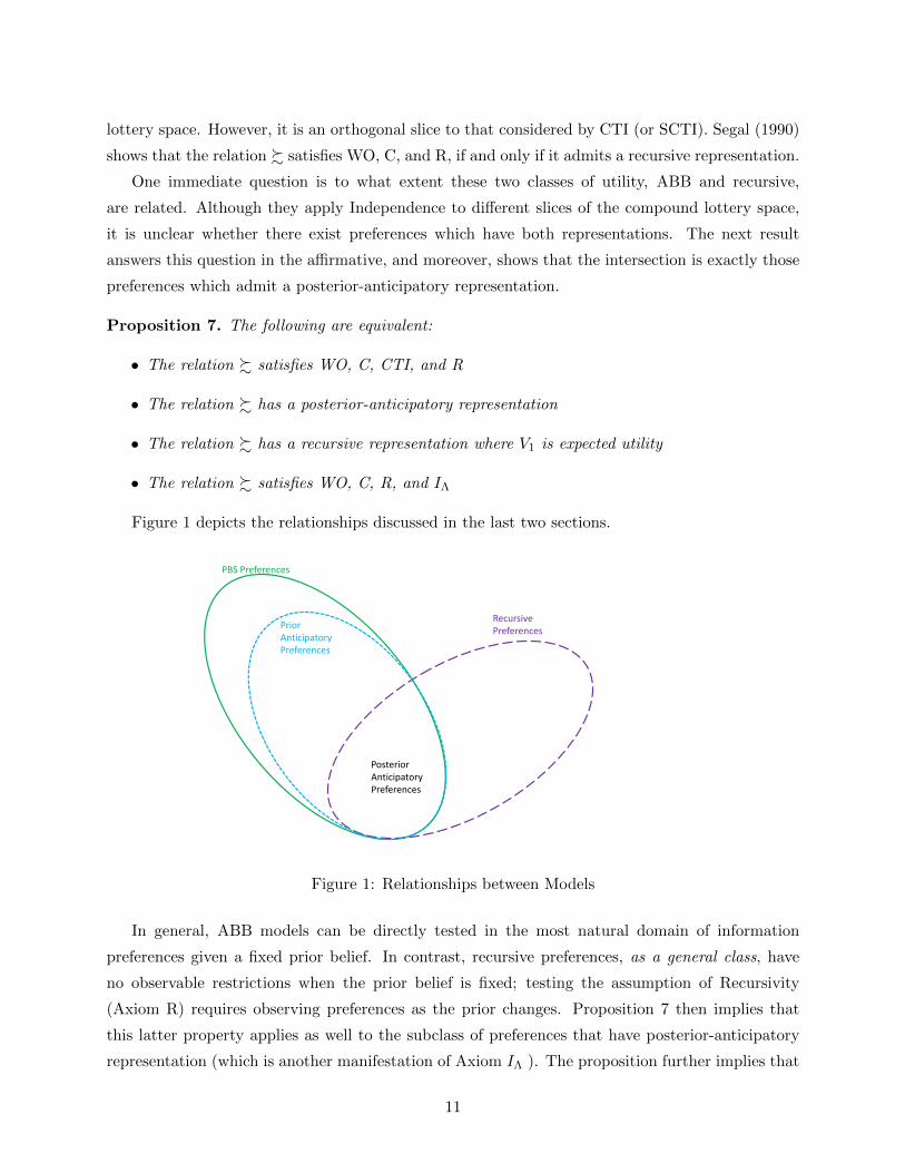
Figure 1 depicts the relationships discussed in the last two sections.

PBS Preferences

PriorAnticipatoryPreferences

RecursivePreferences

Posterior AnticipatoryPreferences

Figure 1: Relationships between Models

In general, ABB models can be directly tested in the most natural domain of information

preferences given a fixed prior belief. In contrast, recursive preferences, as a general class, have

no observable restrictions when the prior belief is fixed; testing the assumption of Recursivity

(Axiom R) requires observing preferences as the prior changes. Proposition 7 then implies that

this latter property applies as well to the subclass of preferences that have posterior-anticipatory

representation (which is another manifestation of Axiom IΛ ). The proposition further implies that

11

any posterior-anticipatory representation captures individuals who have “emotions over emotions”.

This is due to the fact that recursive models transform any two-stage compound lottery into a

simple lottery over the second-stage certainty equivalents. Those certainty equivalents capture all

second-period utility from beliefs changing in the second stage (e.g., disappointment/elation). Since

first-period preferences take the certainty equivalents as the possible outcomes, those anticipated

second period emotions are part and parcel of the “material” payoffs of the first-stage preferences.

In all ABB models which do not have posterior-anticipatory representation, future changes in beliefs

are independent of the effects of previous changes in beliefs. In other words, first period’s beliefs-

based utility, as captured by ν1, is all about changes in material outcomes and does not depend on

second period’s belief-based utility, ν2.

In addition to axiom R, Segal (1990) also introduced several other restrictions on preferences

over compound lotteries (such as the Reduction of Compound Lotteries axiom and the requirement

that Independence holds among both the set of full early resolving lotteries and fully late resolving

lotteries). To complete our analysis, in Appendix 6.3 we establish their relationship with CTI,

SCTI, and TI, and further interpret these connections via the functional forms.

4 ABB and the Timing of Uncertainty Resolution

Individuals with ABB utility will have intrinsic preferences over information, that is, they may

prefer one information structure to another even in the absence of the ability to condition actions

on either of them. Many papers looking at specific examples of ABB functional forms derive results

regarding preferences over information, while focusing on two concepts: preferences for early versus

late resolution of uncertainty and preferences for one-shot versus gradual resolution of uncertainty.

In an analogous vein, characterizations of these informational attitudes have been a major focus of

the decision-theoretic literature. However, there do not exist equivalent characterizations for ABB

preferences. Our results will allow us to compare how different classes of models (recursive and

ABB) can accommodate (or not) different non-instrumental attitudes towards information.

Many authors, such as Kreps and Porteus (1978) and Grant, Kajii, and Polak (1998), conjecture

that individuals not only prefer uncertainty to be fully resolved earlier (in period 1 rather than

in period 2) but also that they always prefer Blackwell-more-informative signals in period 1, that

is, earlier resolution of uncertainty. Drawing on Grant, Kajii, and Polak (1998), we can define a

preference for early resolution of uncertainty.

Definition 7. The relation % displays a preference for early resolution of uncertainty (PERU) if

for any Q,P ∈ ∆2 such that Q = (qi, Q(qi))ni=1, P = ((qi, Q(qi))i 6=j ; p1, βQ(qj); p2, (1 − β)Q(qj))

for some β ∈ [0, 1], and qj = βp1 + (1− β)p2, we have P % Q.

Preference for late resolution of uncertainty is analogously defined, by requiring that for the

12

lotteries above Q % P .

We now characterize preferences that exhibit preferences for either earlier or later resolved

lotteries. Similarly to known results about recursive preferences, attitude towards the resolution of

uncertainty is characterized in our model by the curvature of the appropriate components. In the

next result we refer to preferences which have a prior-anticipatory representation, but do not have

a posterior-anticipatory representation, as having a prior∗- anticipatory representation.

Proposition 8. The following statements are true:

1. Suppose % has ABB representation. Then % exhibits a preference for early (resp., late)

resolution of uncertainty if and only if ν1(ρ, ·) +∑

x ν2(·, x) is convex (resp., concave).

2. Suppose % has a prior∗-anticipatory representation. Then % exhibits a preference for early

(resp., late) resolution of uncertainty if and only if ν2 is convex (resp., concave).

3. Suppose % has a posterior-anticipatory representation. Then % exhibits a preference for early

(resp., late) resolution of uncertainty if and only if ν1 is convex (resp., concave).

A distinct notion of time preferences is discussed by Dillenberger (2010). He supposes that

individuals satisfy Time Neutrality (axiom TN described earlier) and that they prefer either (de-

generate) compound lotteries in which all uncertainty is resolved in period 1 or in period 2 (those

lotteries in Λ or Γ) to any other compound lotteries which induce the same prior beliefs. He defines

this as a preference for one-shot resolution of uncertainty.

Definition 8. The relation % exhibits a preference for one-shot resolution of uncertainty (PORU)

if: (i) % satisfies TN, and (ii) For all P,Q,R ∈ ∆2 such that φ(P ) = φ(Q) = φ(R), if P ∈ Λ and

Q ∈ Γ, then P ∼ Q % R.

In contrast to Proposition 8, the characterization of PORU for general ABB preferences is not

so immediate to interpret. Furthermore, if preferences depend only on the level of beliefs, then

they cannot generate strict PORU. In other words, there are no triple as in Definition 8 for which

P ∼ Q � R hold.

Proposition 9. The following statements are true:

1. Suppose % has ABB representation. Then % exhibits a preference for one shot resolution of

information if and only if

∑x

φ(P )(x)ν1(φ(P ), δx) ≥∑i

P (pi)ν1(φ(P ), pi) +∑pi

P (pi)∑x

pi(x)ν1(pi, δx)

2. If % has a prior-anticipatory representation, then it can never exhibit strict PORU.

13

For item (1), suppose % has ABB representation. If % exhibit PORU then it must have an

ABB representation that satisfies both BSI and BTI, because PORU implies TN. Thus ν1 = ν2.

And since the expected utility from material payoffs is the same in all lotteries compared, the result

follows.8 The intuition behind item (2) derives from Corollary 1, where we show that if % has a

prior-anticipatory representation, then TN implies that ν2 is expected utility. Recall that expected

utility functionals do not generate any anomalous preferences towards information. The rest of

the utility functional depends only on φ, the reduced form probability of the lottery. Moreover,

since we identify anomalous attitudes towards information by using lotteries which all share the

same reduced form probabilities, those other terms always take on the same value, regardless of the

information structure. Thus, we can never observe strict PORU. This is in contrast to recursive

preferences, where Dillenberger (2010) shows that strict PORU can occur and characterizes it in

terms of a single condition on %Γ=%Λ.

5 Discussion

We now discuss how our general framework applies to some specific functional forms used in the

literature. In order to provide a sense of the breadth of models that our approach encompasses,

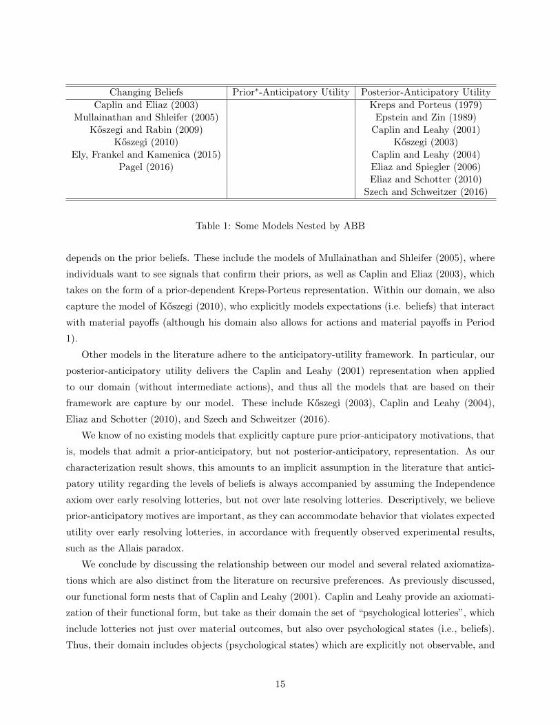
Table 1 provides a list of papers which use functional forms nested by ABB. Many of these models

also allow individuals to take intermediate actions, so their domain and representation may appear

different than that presented in this paper.9

Some models in the literature fit into the framework of changing beliefs models — they have an

ABB representation, but do not have any anticipatory representation. These include models that

are explicitly meant to captures utility derived from changing beliefs, such as Koszegi and Rabin

(2009) and Pagel (2015). Ely, Frankel, and Kamenica (2015) also model individuals who care about

changes in their beliefs. Their model of surprise has the same structure as our ABB representation,

but is formally not within the class of models we study because it is discontinuous. Their model

of suspense is similar in spirit, but formally different from ABB models not only due to it’s lack of

continuity, but also because of a non-linear transformation that is applied to the expected utility

from changes in beliefs. In other models, utility may not be derived from changes in beliefs per

se. Rather, utility is derived from levels of beliefs, but the function that determines the levels

8One example of a function that satisfies PORU is ν1(ρ, p) = −d(ρ, p), where d is some standard distance measureon the unit simplex. In this case, the utility loss from beliefs moving equals the total expected distance traveled bybeliefs. Indeed, for such function the inequality holds term by term (this is the negative of the triangle inequality)and thus also in expectation. One interpretation for such functional form would be that the agent is simply averse toany changes in beliefs, presumably due to some hidden costs of adjustments (think of an agent who pre-committedto some belief-contingent action, or someone who placed bets on his intermediate beliefs) that are ’large enough’,overwhelming any effect of good news.

9As in the previous section, we denote models that have prior-anticipatory but not posterior-anticipatory repre-sentation as having prior∗-anticipatory utility.

14

Changing Beliefs Prior∗-Anticipatory Utility Posterior-Anticipatory Utility

Caplin and Eliaz (2003) Kreps and Porteus (1979)Mullainathan and Shleifer (2005) Epstein and Zin (1989)

Koszegi and Rabin (2009) Caplin and Leahy (2001)Koszegi (2010) Koszegi (2003)

Ely, Frankel and Kamenica (2015) Caplin and Leahy (2004)Pagel (2016) Eliaz and Spiegler (2006)

Eliaz and Schotter (2010)Szech and Schweitzer (2016)

Table 1: Some Models Nested by ABB

depends on the prior beliefs. These include the models of Mullainathan and Shleifer (2005), where

individuals want to see signals that confirm their priors, as well as Caplin and Eliaz (2003), which

takes on the form of a prior-dependent Kreps-Porteus representation. Within our domain, we also

capture the model of Koszegi (2010), who explicitly models expectations (i.e. beliefs) that interact

with material payoffs (although his domain also allows for actions and material payoffs in Period

1).

Other models in the literature adhere to the anticipatory-utility framework. In particular, our

posterior-anticipatory utility delivers the Caplin and Leahy (2001) representation when applied

to our domain (without intermediate actions), and thus all the models that are based on their

framework are capture by our model. These include Koszegi (2003), Caplin and Leahy (2004),

Eliaz and Schotter (2010), and Szech and Schweitzer (2016).

We know of no existing models that explicitly capture pure prior-anticipatory motivations, that

is, models that admit a prior-anticipatory, but not posterior-anticipatory, representation. As our

characterization result shows, this amounts to an implicit assumption in the literature that antici-

patory utility regarding the levels of beliefs is always accompanied by assuming the Independence

axiom over early resolving lotteries, but not over late resolving lotteries. Descriptively, we believe

prior-anticipatory motives are important, as they can accommodate behavior that violates expected

utility over early resolving lotteries, in accordance with frequently observed experimental results,

such as the Allais paradox.

We conclude by discussing the relationship between our model and several related axiomatiza-

tions which are also distinct from the literature on recursive preferences. As previously discussed,

our functional form nests that of Caplin and Leahy (2001). Caplin and Leahy provide an axiomati-

zation of their functional form, but take as their domain the set of “psychological lotteries”, which

include lotteries not just over material outcomes, but also over psychological states (i.e., beliefs).

Thus, their domain includes objects (psychological states) which are explicitly not observable, and

15

not directly choosable. Our approach, which confines attention to preferences over compound lot-

teries, ensures that all our restrictions are stated solely in terms of preferences over observable

objects.

Yariv (2002) also provides a characterization of belief-dependent utility, although in a very

different domain than ours, and for very different purposes. Her work relies on preferences being

expressed over objects where beliefs are independently manipulable across periods. In contrast, our

beliefs in period 2 are not independent of those in period 1.

Recently Gul, Natenzon and Pesendorfer (2016) have introduced a model that shares some key

features of our model. Although the domain and objects of choice are quite different than ours,

there are many key similarities in that both papers consider utility functions where individuals

gain utility from beliefs and from material payoffs in a way that is additively separable. However,

while we suppose individuals calculate the expectation of a belief-based utility using objective

probabilities, Gul, Nautenzon and Pesendorfer (2016) allow for non-additive measures.

6 Appendix

6.1 Proofs

Proof of Lemma 1: By Definition 2, a prior-anticipatory representation is given by∑

i P (pi)∑j pi(xj)u(xj) + ν1(φ(P )) +

∑i P (pi)ν2(pi). Note that preferences admit such a representation if

and only if they can be represented by the functional ν1(φ(P ))+∑

i P (pi)ν2(pi), for some arbitrary

non-expected utility functional ν1. Similarly, by Definition 3, a posterior-anticipatory represen-

tation is given by∑

i P (pi)∑

j pi(xj)[u(xj) + ν2(xj)] +∑

i P (pi)ν1(pi), which is equivalent to a

representation of the form∑

i P (pi)∑

j pi(xj)u(xj) +∑

i P (pi)ν1(pi). Clearly the second represen-

tation is a subset of the first.�

Proof of Proposition 1. We first define a prior-conditional representation as VPC =∑

i P (pi)νPC(φ(P ), pi).

Claim 1. The relation % has a prior-conditional representation if and only if it has an ABB

representation.

Proof of Claim 1. Consider the first two terms in the ABB representation. Observe that the term∑i P (pi)

∑j pi(xj)u(xj)+

∑i P (pi)ν1(φ(P ), pi) can be rewritten as

∑i P (pi)ν1(φ(P ), pi). Similarly,

any∑

i P (pi)ν1(φ(P ), pi) can be rewritten as∑

i P (pi)∑

j pi(xj)u(xj) +∑

i P (pi)ν1(φ(P ), pi).

Consider now the third term in the ABB representation. Note that any∑

i P (pi)∑

j pi(xj)ν2(pi, δxj )

can be rewritten as∑

i P (pi)ν2(pi), since pi embeds all the xjs in it’s support. Moreover, given

any∑

i P (pi)ν2(pi), we can rewrite it as∑

i P (pi)∑

j pi(xj)ν2(pi, δxj ).

Thus preferences have an ABB representation if and only if they can be represented by

16

∑i

P (pi)ν1(φ(P ), pi) +∑i

P (pi)ν2(pi)

Simplifying further, observe that any∑

i P (pi)ν1(φ(P ), pi) +∑

i P (pi)ν2(pi) can be rewritten

as∑

i P (pi)ν(φ(P ), pi); and any∑

i P (pi)ν(φ(P ), pi) can be rewritten as∑

i P (pi)ν1(φ(P ), pi) +∑i P (pi)ν2(pi). We have just proved that % has a representation of the form VABB if and only if

it has a representation of the form∑

i P (pi)ν(φ(P ), pi).

We now use our new representation for Claim 2.

Claim 2. The relation % has a prior-conditional representation if and only if it satisfies WO, C,

and CTI.

Proof of Claim 2. Observe that the prior-conditional representation holds if and only if for any

fixed φ preferences are expected utility, which is known to be equivalent to the three conditions in

the statement of the claim.

This proves the equivalence in the proposition. �

Proof of Proposition 2. First we define a prior-separable representation as VPS = νPS1(φ(P )) +∑i P (pi)νPS2(pi)

Claim 3. The relation % has a prior-separable representation if and only if it has a prior-anticipatory

representation.

Proof of Claim 3. Recall from the proof of Lemma 1 that % has a prior-anticipatory represen-

tation if and only if it has a representation ν1(φ(P )) +∑

i P (pi)ν2(pi). Note that this is simply the

sum of a utility function defined over the reduced lottery and a recursive utility that is expected

utility in the first stage.

We now use our new representation for Claim 4.

Claim 4. The relation % has a prior-separable representation if and only if it satisfies WO, C,

and SCTI.

Proof of Claim 4. It is easy to check that the axioms are necessary for the representation. For

sufficiency, observe that SCTI implies CTI, which, in turns, implies that there exists a representation

of the form∑

i P (pi)ν(φ(P ), pi). Moreover, by SCTI, if∑

i P (pi)ν(φ(P ), pi) =∑

iQ(pi)ν(φ(P ), pi),

then∑

i(αP + (1 − α)R)(pi)ν(φ((αP + (1 − α)R)), pi) =∑

i(αQ + (1 − α)R)(pi)ν(φ((αP + (1 −α)R)), pi) for any R, which is true if and only if ν is additively separable in it’s first argument:

17

∑i P (pi)ν(φ(P ), pi) = ν1(φ(P ))+

∑i P (pi)ν2(pi). To see this, observe that with n sub-lotteries, the

utility function VPS can be thought of as a function of n+1 arguments — the n sub-lotteries and the

prior beliefs. Since the representation is additively separable,conditional on the prior, preferences

must satisfy separability (i.e, preferential independence in Debreu, 1960) across the sub-lotteries

(and all subsets of the sub-lotteries). Further observe that SCTI implies that all subsets of the

sub-lotteries and the prior also satisfy separability (preferential independence). Thus, by Debreu

(1960) (see also Wakker, 1993) the representation must be additively separable in all components.

This proves the equivalence in the proposition. �

Proof of Proposition 3. First we define a prior-separable expected utility representation as

VPSEU =∑

x φ(P )(x)νPSEU1(x) +∑

i P (pi)νPSEU2(pi).

Claim 5. The relation % has a prior-separable expected utility representation if and only if it has

a posterior-anticipatory representation.

Proof of Claim 5. From Lemma 1, % has a posterior-anticipatory representation if and only if

it has a representation∑

i P (pi)∑

j pi(xj)u(xj) +∑

i P (pi)ν1(pi). This is simply the sum of a an

expected utility function defined over the reduced lottery and a recursive utility that is expected

utility in the first stage.

We now use the new representation for Claim 6.

Claim 6. The relation % has a prior-separable expected utility representation if and only if it

satisfies WO, C, SCTI, and IΛ.

Proof of Claim 6. It is easy to check that any VPSEU representation satisfies SCTI and IΛ.

For the other direction, notice that we have (given SCTI) a representation of the form ν1(φ(P )) +∑i P (pi)ν2(pi). Moreover, IΛ implies that Independence is satisfied over lotteries in Λ. Observe

that within Λ the representation has the form ν1(φ(P )) +∑

i P (δxi)ν2(δxi). The second terms is

simply an expected utility functional on Λ. Thus, the first term must be expected utility over the

reduced form probabilities in order for Independence to be satisfied.

Claim 7. The relation % has a prior-separable expected utility representation if and only if it

satisfies WO, C and TI.

Observe that by the mixture space theorem, % satisfies WO, C, and TI if and only if it

can be represented by the functional∑

i P (pi)ν(pi). Moreover, if preferences can be represented

by∑

i P (pi)ν(pi) then clearly they have a prior-separable expected utility representation (where

18

νPSEU1(x) = 0). Similarly, any prior anticipatory representation can be written as∑

i P (pi)ν(pi)

where ν(pi) = νPSEU2(pi) +∑

x pi(x)νPSEU1(x).

This proves the equivalence in the proposition. �

Proof of Proposition 4. We prove each of the statements in order.

• We first show that if % has an ABB representation then it has a BSI representation in a series

of two claims.

Claim 8. There exists an equivalent representation (u, ν1, ν2) which satisfies the condition

ν1(ρ, ρ) = 0 for all ρ.

Proof of Claim 8. Denote as N(p) the number of elements in the support of p and

sum up below only amongst those elements with positive probability. Define: ν1(ρ, p) =

ν1(ρ, p)−ν1(p, p) and ν2(p, δx) = ν2(p, δx)+ ν1(p,p)N(p)p(x) . By construction, ν1(ρ, ρ) = 0. Moreover,

preferences did not change as the new representation gives utility:

∑x

ρ(x)u(x) +∑p

P (p)ν1(ρ, p) +∑p

∑x

P (p)p(x)ν2(p, δx)

or

∑x

ρ(x)u(x) +∑p

P (p)[ν1(ρ, p)− ν1(p, p)] +∑p

∑x

P (p)p(x)[ν2(p, δx) +ν1(p, p)

N(p)p(x)]

or

∑x

ρ(x)u(x)+∑p

P (p)ν1(ρ, p)−∑p

P (p)ν1(p, p)+∑p

∑x

P (p)p(x)ν2(p, δx)+∑p

P (p)ν1(p, p)∑x

1

N(p)

or

∑x

ρ(x)u(x)+∑p

P (p)ν1(ρ, p)−∑p

P (p)ν1(p, p)+∑p

P (p)ν1(p, p)+∑p

∑x

P (p)p(x)ν2(p, δx)

which is the original utility function.�

Claim 9. There exists an equivalent representation (u, ν1, ν2), which satisfies the condition

ν2(δx, δx) = 0 for all x ∈ X.

19

Proof of Claim 9. Define ν2(p, δx) = ν2(p, δx) − ν2(δx, δx) and u(x) = u(x) + ν2(δx, δx).

Note that ν2(δx, δx) = 0 for all x. Observe that this does not change preferences since utility

under this representation is:

∑x

u(x)ρ(x) +∑p

P (p)ν1(ρ, p) +∑p

∑x

P (p)p(x)ν2(p, δx)

or

∑x

ρ(x)[u(x) + ν2(δx, δx)] +∑p

P (p)ν1(ρ, p) +∑p

P (p)p(x)[ν2(p, δx)− ν2(δx, δx)]

or

∑x

ρ(x)u(x)+∑p

P (p)ν1(ρ, p)+∑p

∑x

P (p)p(x)ν2(p, δx)+∑x

ρ(x)ν2(δx, δx)−∑p

∑x

P (p)p(x)ν2(δx, δx)

which is simply the original utility function.�

Thus, we have a utility representation (u, ν1, ν2) which satisfied BSI.

• We next show that % always has a representation which is belief-time invariant. Take the

representation (u, ν1, ν2) defined in the previous part. Define

ν ′2(p, δx) = ν2(p, δx) + [ν1(p, δx)− ν2(p, δx)]

and

ν ′1(ρ, p) = ν1(ρ, p)−∑x

p(x)[ν1(p, δx)− ν2(p, δx)]

Observe (u, ν ′1, ν′2) represents the same preferences. Utility under the second representation

is:

∑x

u(x)ρ(x) +∑p

P (p)ν ′1(ρ, p) +∑p

∑x

P (p)p(x)ν ′2(p, δx)

20

or

∑x

u(x)ρ(x) +∑p

P (p)[ν1(ρ, p)−∑x

p(x)[ν1(p, δx)− ν2(p, δx)]]

+∑p

∑x

P (p)p(x)[ν2(p, δx) + [ν1(p, δx)− ν2(p, δx)]]

or

∑x

u(x)ρ(x) +∑p

P (p)ν1(ρ, p)−∑p

∑x

P (p)p(x)[ν1(p, δx)− ν2(p, δx)]

+∑p

∑x

P (p)p(x)ν2(p, δx) +∑p

∑x

P (p)p(x)[ν1(p, δx)− ν2(p, δx)]

or ∑x

u(x)ρ(x) +∑p

P (p)ν1(ρ, p) +∑p

∑x

P (p)p(x)ν2(p, δx)

which are the original preferences.

Moreover, observe that by construction

ν ′1(p, δx) = ν1(p, δx)− [ν1(δx, δx)− ν2(δx, δx)] = ν1(p, δx)− [0− 0]

Also

ν ′2(p, δx) = ν2(p, δx) + [ν1(p, δx)− ν2(p, δx)] = ν1(p, δx)

Thus we satisfy BTI. However, we no longer satisfy BSI. This is because

ν ′1(ρ, ρ) = ν1(ρ, ρ)−∑x

ρ(x)[ν1(ρ, δx)− ν2(ρ, δx)]

no longer necessarily equals 0.

• We now show that % has a representation which is both belief-stationary invariant and belief-

time invariant if and only if it satisfies TN.

For the only if part, observe that for P ∈ Γ

VABB(P ) = Eφ(P )(u) + ν1(φ(P ), φ(P )) +∑j

φ(P )(xj)ν2(φ(P ), δxj )

= Eφ(P )(u) +∑j

φ(P )(xj)ν2(φ(P ), δxj )

where the second equality is by BSI.

21

For Q ∈ Λ we have

VABB(Q) = Eφ(Q)(u) +∑j

φ(Q)(xj)ν1(φ(Q), δxj ) +∑j

φ(Q)(xj)ν2(δxj , δxj )

= Eφ(Q)(u) +∑j

φ(Q)(xj)ν1(φ(Q), δxj )

where the second equality is again by BSI.

By BTI,∑

j φ(P )(xj)ν2(φ(P ), δxj ) =∑

j φ(Q)(xj)ν1(φ(Q), δxj ). And if φ(P ) = φ(Q), then

indeed VABB(P ) = VABB(Q), that is, TN is satisfied.

To prove the other direction, we can simply assume preferences satisfy BSI. Observe that

time neutrality implies that

∑x

u(x)ρ(x)+ν1(ρ, ρ)+∑x

ρ(x)ν2(ρ, δx) =∑x

u(x)ρ(x)+∑x

ρ(x)ν1(ρ, δx)+∑x

ρ(x)ν2(δx, δx)

or, taking the fact that BSI holds

∑x

ρ(x)ν2(ρ, δx) =∑x

ρ(x)ν1(ρ, δx)

Observe that ν1(ρ, δx) only appears as a term as part of the sum∑

x ρ(x)ν1(ρ, δx). Thus, we

cannot separately identify the individual parts of∑

x ρ(x)ν1(ρ, δx). Since∑

x ρ(x)ν2(ρ, δx) =∑x ρ(x)ν1(ρ, δx) we can simply suppose without loss of generality that ρ(x)ν2(ρ, δx) = ρ(x)ν1(ρ, δx)

term by term.

• Lastly, as we mention in Footnote 2, we show that if % has an ABB representation, then it has

a representation which is both belief-stationary invariant and pseudo-belief-time invariant.10

First, normalize the representation using claims 8 and 9 so that it satisfies BSI. We then

normalize the representation so that BTI holds as in the second part of the proof of this

proposition. As we have mentioned there, ν ′1(ρ, ρ) no longer necessarily equals 0. But, since

we started with a BSI representation, we already had that ν ′1(δx, δx) = ν ′2(δx, δx) = 0 so those

values do not change.

In order to simplify notation, call the functionals after these two steps u, ν1, and ν2 respec-

tively. Thus, ν1 = ν2 over their shared domain, and ν2(δx, δx) = 0 = ν1(δx, δx).

10Since % always has a representation which is belief-time invariant. This immediately implies that there is also aPBTI representation, where κ = 1.

22

Now we will define a representation that satisfies both BSI and PBTI. We do this in a way

that mirrors Claim 8. Denote as N(p) the number of elements with positive probability in

p and sum up below only amongst those elements. Define: ν1(ρ, p) = ν1(ρ, p) − ν1(p, p).

Importantly, this redefinition implies ν1(ρ, δx) = ν1(ρ, δx)− ν1(δx, δx) = ν1(ρ, δx).

We then turn to solve for ν2. Denote z(p) = ν1(p, p). For our representation to satisfy

PBTI we need that ν2(p, δx) = κν1(p, δx) = κν1(p, δx) = κν2(p, δx) for some κ. If p has N(p)

outcomes in its support, then these are N(p) equations and N(p)+1 unknowns. We also need

it to be the case that∑p(x)ν2(p, δx) = z(p). Substituting in we get κ

∑p(x)ν2(p, δx) = z(p)

or κ = z(p)∑p(x)ν2(p,δx) . Observe that this uniquely pins down κ and so uniquely pins down ν2

for each p. Thus, PBTI is satisfied. Moreover, observe that by construction ν2(δx, δx) = 0

still and ν1(ρ, ρ) = 0, and so BSI is satisfied as well.

�

Proof of Proposition 5. From Claim 1 we know that we can confine attention to a prior-

conditional representation of %. Observe that fixing φ(P ),∑

i P (pi)νPC(φ(P ), pi) is an expected

utility functional, and so possesses the same uniqueness results; i.e. it is unique up to affine trans-

formations of scalars αP > 0 and βP . But, since∑

i P (pi)νPC(φ(P ), pi) ≥∑

iQ(qi)νPC(φ(Q), qi) if

and only if βP + αP∑

i P (pi)νPC(φ(P ), pi) ≥ βQ + αQ∑

iQ(qi)νPC(φ(Q), qi), it must be the case

that βP = βQ and αP = αQ. �

Proof of Proposition 6. To see the result for a BSI representation, first take the uniqueness

result for general ABB preferences (Proposition 10 in Appendix 6.2). Suppose that (u, ν1, ν2) is

a BSI representation. We first show that any transformation where γ1(x) 6= 0 for some x cannot

generate a BSI representation. Suppose that there is some xi such that γ1(xi) 6= 0. Consider the

two-stage lottery Dδxi. Then ν ′1(δxi , δxi) = 0 − γ1(xi) 6= 0 so this cannot be a BSI representation.

Next we show that any transformation where γu(x) 6= 0 for some x cannot generate a BSI rep-

resentation. Suppose that there is some xi such that γu(xi) 6= 0. Consider the two-stage lottery

Dδxi. Then ν ′2(δxi , δxi) = 0 − γu(xi) 6= 0 so this cannot be a BSI representation. For similar

resasons β1 = β2 = 0. Lastly, we show that any transformation where γν(p, δx) 6= 0 for some p

and x cannot generate a BSI representation. If there were pi and xj such that γν(pi, δxj ) 6= 0, then

ν ′1(p, p) = 0 + p(x)γν(pi, δxj ) 6= 0, violating a BSI representation. �

Proof of Proposition 7. We first show that % has a posterior-separable expected utility

representation (i.e. it satisfies WO, C, SCTI, and IΛ) if and only if it satisfies WO, C, CTI, and R.

Necessity is immediate. To show sufficiency, note that we have a representation of the form

VPC =∑

i P (pi)νPC(φ(P ), pi). If recursivity is satisfied, then it must be the case that νPC is

23

independent of the first argument. Thus we have a representation of the form∑

i P (pi)νPC(pi),

which is equivalent to the following representation:∑

i P (pi)∑

j pi(xj)u(xj) +∑

i P (pi)ν1(pi).

Recall that % has a posterior-anticipatory representation if and only if it has a representation∑i P (pi)ν(pi). By Segal (1990), this is a recursive representation where V1 is expected utility. Segal

(1990) also shows that this representation holds if and only if % satisfies WO, C, R and IΛ. �

Proof of Proposition 8. For item (1), observe that we can ignore the first term of the ABB

representation, as it is the same under any two compound lotteries with the same reduced form

probabilities. Suppose then that ν1(ρ, ·) +∑

x ν2(·, x) is convex. Then, by Grant, Kajii and Polak

(1998) the individual must exhibit a preference for early resolution of uncertainty. Conversely, if

the term above is not convex, then it must be concave in a local neighborhood of some pi. We

can replicate the argument in Grant, Kajii and Polak (1998). Take some compound lottery that

delivers as one sub-lottery pi, and take a linear bifurcation of pi so that the new sub-lotteries are

arbitrarily close to pi. Then by Grant, Kajii and Polak (1998) the individual must be worse off

(since locally the utility function is concave).

For item (2), take any P and Q as specified in the statement of the proposition. Observe that

φ(P ) = φ(Q). Direct calculations then show that P % Q if and only if βν2(p1) + (1 − β)ν2(p2) ≥ν2(βp1 + (1 − β)p2). And since the triple p1, p2, and β were arbitrary, the inequality holds if and

only if ν2 is convex. Similarly, the inequality is reversed if and only if ν2 is concave.

For item (3), simply replace in the entire paragraph above ν2 with ν1. �

6.2 Uniqueness of ABB representations

In this section we present more detailed uniqueness results.

Proposition 10. Suppose % has an ABB representation (u, ν1, ν2). The ABB representation

(u′, ν ′1, ν′2) also represents % if and only if there exists scalars α > 0, βu, β1, β2, and continuous

functions γu : X → R, γ1 : X → R, and γν : ∆×X → R such that

• u′(x) = αu(x) + βu + γu(x) + γ1(x)

• ν ′1(ρ, p) = αν1(ρ, p) + β1 +∑

x p(x)γν(p, δx)−∑

x ρ(x)γ1(x)

• ν ′2(p, δx) = αν2(p, δx) + β2 − γν(p, δx)− γu(x)

Proof of Proposition 10. We first show that if

• u′(x) = αu+ βu + γu(x) + γ1(x)

• ν ′1(ρ, p) = αν1(ρ, p) + β1 +∑

x p(x)γν(p, δx)−∑

x ρ(x)γ1(x)

• ν ′2(p, δx) = αν2(p, δx) + β2 − γν(p, δx)− γu(x)

24

then (u′, ν ′1, ν′2) represents the same preferences as (u, ν1, ν2).

Consider the utility function generated by the former representation.

∑x

u′ρ(x) +∑p

P (p)ν ′1(ρ, p) +∑p

∑x

P (p)p(x)ν ′2(p, δx)

or

∑x

ρ(x)[αu+ βu + γu(x) + γ1(x)]

+∑p

P (p)[αν1(ρ, p) + β1 +∑x

p(x)γν(p, δx)−∑x

ρ(x)γ1(x)]

+∑p

∑x

P (p)p(x)[αν2(p, δx) + β2 − γν(p, δx)− γu(x)]

or

α∑x

ρ(x)u+ βu +∑x

ρ(x)γu(x) +∑x

ρ(x)γ1(x)

+ α∑p

P (p)ν1(ρ, p) + β1 +∑p

∑x

P (p)p(x)γν(p, δx)−∑p

P (p)∑x

ρ(x)γ1(x)

+ α∑p

∑x

P (p)p(x)ν2(p, δx) + β2 −∑p

∑x

P (p)p(x)γν(p, δx)−∑p

∑x

P (p)p(x)γu(x)

Denoting β = βu + β1 + β2 and recalling that∑

p

∑x P (p)p(x) =

∑x ρ(x) we get

α[∑x

ρ(x)u+∑p

P (p)ν1(ρ, p) +∑p

∑x

P (p)p(x)ν2(p, δx)] + β

+∑x

ρ(x)γu(x) +∑p

∑x

P (p)p(x)γν(p, δx) +∑x

ρ(x)γ1(x)

−∑p

∑x

P (p)p(x)γν(p, δx)−∑x

ρ(x)γu(x)−∑x

ρ(x)γ1(x)

or

α[∑x

ρ(x)u+∑p

P (p)ν1(ρ, p) +∑p

∑x

P (p)p(x)ν2(p, δx)] + β

which clearly are the same preferences as (u, ν1, ν2).

To prove the other direction, suppose that (u, ν1, ν2) and (u′, ν ′1, ν′2) represent the same prefer-

25

ences.

Define u(x) = u(x)−u(x); ν2(p, δx) = ν2(p, δx)−ν2(p, δx); and ν1(ρ, p) = ν1(ρ, p)+∑

x ρ(x)u(x)+∑x p(x)ν2(p, δx). These represent the same preferences as (u, ν1, ν2) but we can write V (P ) =∑p P (p)ν1(φ(P ), p).

Now define u′(x) = u′(x) − u′(x); ν ′2(p, δx) = ν ′2(p, δx) − ν ′2(p, δx); and ν ′1(ρ, p) = ν ′1(ρ, p) +∑x ρ(x)u′(x) +

∑x p(x)ν ′2(p, δx). These represent the same preferences as (u′, ν ′1, ν

′2) but we can

write V ′(P ) =∑

p P (p)ν ′1(φ(P ), p).

Since V (P ) =∑

p P (p)ν1(φ(P ), p) and V ′(P ) =∑

p P (p)ν ′1(φ(P ), p) we know that ν ′1(φ(P ), p)

must be an affine transformation of ν1(φ(P ), p) ; so that ν ′1(φ(P ), p) = αν1(φ(P ), p) + β. Thus

V ′(P ) =∑

p P (p)αν1(φ(P ), p) + β. Clearly,∑

p αP (p)ν1(φ(P ), p) + β has an ABB representation

(αu+ βu, αν1 + β1, αν2 + β2), where βu + β1 + β2 = β.

By construction αu = u′ = 0 and αν2 = ν ′2 = 0. Thus we can say u′(x) = u′(x)−αu(x)+αu(x);

ν ′2(p, δx) = ν ′2(p, δx) − αν2(p, δx) + αν2(p, δx); and ν ′1(φ(P ), p) = αν1(φ(P ), p) −∑

x ρ(x)[u′(x) −αu(x)] −

∑x p(x)[ν ′2(p, δx) − αν2(p, δx)] + β. Moreover, it is easy to verify that we can arbitrarily

divide β among the terms.

Define γu(x) = 0; γ1(x) = u′(x) − αu(x); and γν(p, δx) = −[ν ′2(p, δx) − αν2(p, δx)]. Then

u′(x) = αu(x) + γu(x) + γ1(x)βu; ν ′2(p, δx) = αν2(p, δx)− γν(p, δx)− γu(x) + β1 and ν ′1(φ(P ), p) =

αν1(φ(P ), p) +∑

x p(x)γν(p, δx)−∑

x ρ(x)γ1(x). Thus we have constructed the transformation.�

For completeness, we now show that if we suppose utility depends only on the levels of beliefs,

stronger uniqueness results also obtain. In this case, both belief-based functionals are unique up to

expected utility preferences. Thus, the only part of the utility function not uniquely identified (up

to standard transformations) are an individual’s expected utility attitudes towards final outcomes.

Proposition 11. Suppose % has an anticipatory representation (u, ν1, ν2). The ABB representation

(u′, ν ′1, ν′2) also represents % if and only if there are scalars α > 0, βu, β1, β2 and continuous functions

γu : X → R and γν : X → R such that

• u′(x) = αu+ βu + γu(x) + γν(x)

• ν ′1(ρ) = αν1(ρ) + β1 −∑

x ρ(x)γν(x)

• ν ′2(p) = αν2(p) + β2 −∑p(x)γu(x)11

Proof of Proposition 11. The proof is analogous to the one of Proposition 10. We show

necessity for prior anticipatory preferences as an example. Consider the utility function generated

by the latter representation.

∑x

u′ρ(x) +∑p

P (p)ν ′1(ρ) +∑p

∑x

P (p)p(x)ν ′2(p)

11Observe that in a posterior-anticipatory representation p is a degenerate lottery.

26

or

∑x

ρ(x)[αu(x) + βu + γu(x) + γν(x)] +∑p

P (p)[αν1(ρ) + β1 −∑x

ρ(x)γν(δx)]

+∑p

∑x

P (p)p(x)[αν2(p) + β2 − γu(x)]

or

α∑x

ρ(x)u(x) + βu +∑x

ρ(x)γu(x) +∑x

ρ(x)γν(x) + αν1(ρ) + β1 −∑x

ρ(x)γν(δx)

+∑p

P (p)αν2(p) + β2 −∑p

∑x

P (p)p(x)γu(x)

Denoting β = βu + β1 + β2 and recalling that∑

p

∑x P (p)p(x) =

∑x ρ(x) we get

α[∑x

ρ(x)u(x) + ν1(ρ) +∑p

P (p)αν2(p)] + β

which clearly are the same preferences as (u, ν1, ν2). �

6.3 ABB and Recursive Preferences: Other Properties

In addition to axiom R, Segal (1990) also introduced several other restrictions on preferences over

compound lotteries. We first quickly review them. The strongest assumption is called Reduction of

Compound Lotteries (ROCL), which supposes that individuals only care about the reduced form

probabilities of any given compound lottery.

Reduction of Compound Lotteries (ROCL): For all P,Q ∈ ∆2, if φ(P ) = φ(Q) then P ∼ Q.

Another assumption is to apply Independence not just to the set of full early resolving lotteries

(Axiom IΛ) but also to the set of fully late resolving lotteries. This restriction, which we denote

by IΓ, says that %Γ satisfies Independence.

Independence (I): Both IΛ and IΓ hold.

A third assumption is Time Neutrality (TN), discussed in the previous section.

Segal (1990), among other things, relates his proposed axioms to one another. In particular, he

shows that if % satisfies WO and C, then (i) ROCL implies TN; (ii) ROCL and R imply I, and

ROCL and I imply R; and (iii) R, I, and TN, imply ROCL. We can extend Segal’s reasoning to

include CTI, SCTI, and TI.

27

Proposition 12. Suppose % satisfies WO and C. The following statements are true.12

1. (i) ROCL implies TI; (ii) TI implies SCTI; (iii) SCTI implies CTI.

2. (i) R and CTI jointly imply TI (and so SCTI); (ii) SCTI and TN jointly imply ROCL

3. TN, R, and CTI jointly imply I (and so ROCL).

Proof of Proposition 12. We show each part in turn

1. Observe that ROCL implies that all lotteries with the same reduce form probabilities are

indifferent, which immediately implies TI. It’s clear that TI implies SCTI which implies CTI.

2. R and CTI have been already shown to imply a posterior-anticipatory representation, which

implies TI (and so SCTI). SCTI implies that we have a representation of the form ν1(φ(P ))+∑i P (pi)ν2(pi). Over early resolving lotteries this takes the structure ν1(φ(P ))+

∑i P (δxi)ν2(δxi),

which is simply a non-expected utility functional over the reduced form probabilities. TN

implies this must true true also for any lottery with structure ν1(φ(P )) + ν2(φ(P )), and so

ν2(φ(P )) = sumiP (δxi)ν2(δxi), and so ν2 satisfies reduction, and so ROCL is satisfied.

3. Last, observe that R and CTI imply that SCTI must be satisfied, and we know that SCTI

and TN imply ROCL. �

All relationships in Proposition 12 are interpreted via the lens of restrictions on preferences. In

the context of our paper, it is perhaps more instructive to interpret them via the functional forms.

Corollary 1. Suppose % has a prior-anticipatory representation. Then (i) TN or ROCL implies

that ν2 is an expected utility function; and (ii) R or IΛ implies that % has a posterior-anticipatory

representation.

If % has a posterior-anticipatory representation and satisfies TN, then it is expected utility.

Proof of Corollary 1: A prior-anticipatory representation implies that SCTI is satisfied. From the

previous proof we know that SCTI and TN jointly imply ROCL, and that ROCL alone implies TN.

Given the representation ν1(φ(P )) +∑

i P (pi)ν2(pi), TN implies that ν2(p) = sumip(δxi)ν2(δxi),

and so ν2 is expected utility. If IΛ or R is satisfied then a posterior-anticipatory representation is

implied.

The representation of posterior-anticipatory preferences has the form∑

i P (pi)∑

j pi(xj)u(xj)+∑i P (pi)ν1(pi). Observe that over Λ these preferences have the structure

∑i P (pi)

∑j pi(xj)u(xj)+∑

i P (δxi)ν1(δxi), which is expected utility. Thus, if TN is satisfied, preferences over Γ must also

satisfy Independence. �

12Items 1(iii) and 2(i) have already been established earlier; we add them here for completeness.

28

References

[1] Gregory S Berns, Jonathan Chappelow, Milos Cekic, Caroline F Zink, Giuseppe Pagnoni, andMegan E Martin-Skurski. Neurobiological substrates of dread. Science, 312(5774):754–758,2006.

[2] Andrew Caplin and Kfir Eliaz. Aids policy and psychology: A mechanism-design approach.RAND Journal of Economics, pages 631–646, 2003.

[3] Andrew Caplin and John Leahy. Psychological expected utility theory and anticipatory feel-ings. The Quarterly Journal of Economics, 116(1):55–79, 2001.

[4] Andrew Caplin and John Leahy. The supply of information by a concerned expert. TheEconomic Journal, 114(497):487–505, 2004.

[5] Gerard Debreu. Mathematical methods in the social sciences, chapter Topological methods incardinal utility theory. Stanford University Press, Stanford, 1960.

[6] David Dillenberger. Preferences for one-shot resolution of uncertainty and Allais-type behavior.Econometrica, 78(6):1973–2004, 2010.

[7] Kfir Eliaz and Andrew Schotter. Paying for confidence: An experimental study of the demandfor non-instrumental information. Games and Economic Behavior, 70(2):304–324, 2010.

[8] Kfir Eliaz and Ran Spiegler. Can anticipatory feelings explain anomalous choices of informationsources? Games and Economic Behavior, 56(1):87–104, 2006.

[9] Jeffrey Ely, Alexander Frankel, and Emir Kamenica. Suspense and surprise. Journal of PoliticalEconomy, 123(1):215–260, 2015.

[10] Larry G Epstein and Stanley E Zin. Substitution, risk aversion, and the temporal behavior ofconsumption and asset returns: A theoretical framework. Econometrica, pages 937–969, 1989.

[11] Simon Grant, Atsushi Kajii, and Ben Polak. Intrinsic preference for information. Journal ofEconomic Theory, 83(2):233–259, 1998.

[12] Faruk Gul, Paulo Natenzon, and Wolfgang Pesendorfer. Random evolving lotteries and intrinsicpreference for information. Technical report, 2016.

[13] Botond Koszegi and Matthew Rabin. Reference-dependent consumption plans. The AmericanEconomic Review, 99(3):909–936, 2009.

[14] Botond Koszegi. Health anxiety and patient behavior. Journal of health economics, 22(6):1073–1084, 2003.

[15] David M Kreps and Evan L Porteus. Temporal resolution of uncertainty and dynamic choicetheory. Econometrica, pages 185–200, 1978.

[16] Richard S Lazarus. Psychological stress and the coping process. 1966.

[17] George Loewenstein. Anticipation and the valuation of delayed consumption. The EconomicJournal, 97(387):666–684, 1987.

29

[18] Sendhil Mullainathan and Andrei Shleifer. The market for news. American Economic Review,pages 1031–1053, 2005.

[19] Michaela Pagel. A news-utility theory for inattention and delegation in portfolio choice. Work-ing Paper, 2016.

[20] Todd Sarver. Optimal reference points and anticipation. Technical report, Discussion Paper,Center for Mathematical Studies in Economics and Management Science, 2012.

[21] Nikolaus Schweizer and Nora Szech. Optimal revelation of life-changing information. Workingpaper, 2016.

[22] Uzi Segal. Two-stage lotteries without the reduction axiom. Econometrica, pages 349–377,1990.

[23] Peter Wakker. Additive representations on rank-ordered sets: Ii. the topological approach.Journal of Mathematical Economics, 22(1):1–26, 1993.

[24] Leeat Yariv. Believe and let believe:axiomatic foundations for belief dependent utility func-tionals. Technical report, 2001.

30