advanced aeroelastic simulations for practical fixed-wing
TRANSCRIPT
Advanced Aeroelastic Simulations for Practical Fixed-wing and Rotary-wing Applications
by
Sean A. M. McTavish
A Thesis submitted to
the Faculty of Graduate Studies and Research
in partial fulfilment of
the requirements for the degree of
Master of Applied Science
Ottawa-Carleton Institute for
Mechanical and Aerospace Engineering
Department of Mechanical and Aerospace Engineering
Carleton University
Ottawa, Ontario, Canada
September 2008
Copyright ©
2008 - Sean A. M. McTavish

1*1 Library and Archives Canada
Published Heritage Branch
395 Wellington Street Ottawa ON K1A0N4 Canada
Bibliotheque et Archives Canada
Direction du Patrimoine de I'edition
395, rue Wellington Ottawa ON K1A0N4 Canada
Your file Votre reference ISBN: 978-0-494-44052-0 Our file Notre reference ISBN: 978-0-494-44052-0
NOTICE: The author has granted a nonexclusive license allowing Library and Archives Canada to reproduce, publish, archive, preserve, conserve, communicate to the public by telecommunication or on the Internet, loan, distribute and sell theses worldwide, for commercial or noncommercial purposes, in microform, paper, electronic and/or any other formats.
AVIS: L'auteur a accorde une licence non exclusive permettant a la Bibliotheque et Archives Canada de reproduire, publier, archiver, sauvegarder, conserver, transmettre au public par telecommunication ou par Plntemet, prefer, distribuer et vendre des theses partout dans le monde, a des fins commerciales ou autres, sur support microforme, papier, electronique et/ou autres formats.
The author retains copyright ownership and moral rights in this thesis. Neither the thesis nor substantial extracts from it may be printed or otherwise reproduced without the author's permission.
L'auteur conserve la propriete du droit d'auteur et des droits moraux qui protege cette these. Ni la these ni des extraits substantiels de celle-ci ne doivent etre imprimes ou autrement reproduits sans son autorisation.
In compliance with the Canadian Privacy Act some supporting forms may have been removed from this thesis.
Conformement a la loi canadienne sur la protection de la vie privee, quelques formulaires secondaires ont ete enleves de cette these.
While these forms may be included in the document page count, their removal does not represent any loss of content from the thesis.
Canada
Bien que ces formulaires aient inclus dans la pagination, il n'y aura aucun contenu manquant.
Abstract
The study of aeroelasticity has many applications in the aerospace industry. There is
a need in the fixed-wing and rotary-wing fields to develop computational aeroelastic
tools for industrial applications that are both rapid and robust. Aeroelastic tools
that would benefit the industry were developed in this work to predict the transonic
fixed-wing flutter boundary and to predict rotary-wing wind turbine performance.
The flutter boundary of a wing must be determined during development and
certification of an aircraft, and is critical in the transonic regime, where nonlinear
effects create a dip in the flutter boundary that cannot be predicted with traditional
linear tools. A frequency domain correction procedure was developed to account
for nonlinear aerodynamics in the transonic regime. The flutter boundary of the
experimental benchmark AGARD 445.6 wing was calculated using time domain and
corrected frequency domain methods. Both approaches adequately predicted the
flutter boundary, but the corrected frequency domain approach is significantly faster
than the time domain simulations and represents a unique opportunity for improved
flutter prediction during aircraft wing design and development.
Wind turbines represent a rapidly growing source of renewable energy but current
predictive tools have been shown to lack accuracy in predicting the power output
of wind turbines. Additionally, wind farm performance must be properly predicted
to develop accurate annual energy estimates. An aeroelastic, aeroacoustic, discrete
vortex method code called SMARTROTOR was used to predict the performance of
the benchmark National Renewable Energy Laboratory (NREL) wind turbine exper
iment. The code properly predicted the NREL wind turbine performance in normal
and yawed flow conditions and has demonstrated the capability of simulating the wake
interference effects present in wind farms. The grid-free characterization of the wake
behind the turbine and the rapid simulation time compared with grid-based com
putational fluid dynamics solvers highlights the relevance of the code for industrial
applications.

This thesis is dedicated to my grandmothers and the inspiration they have provided.
IV
Acknowledgments
I would like to thank Dr. Daniel Feszty and Dr. Fred Nitzsche for their support
and encouragement throughout this project. Thank you to all of the professors in
the Mechanical and Aerospace Engineering department at Carleton who have been
wonderful teachers and mentors and to Nancy Powell, Marlene Groves, and Christie
Egbert, whose help has been invaluable throughout my undergraduate and graduate
degrees. I would like to extend my appreciation to Dr. Slavik and my colleagues at
the Czech Technical University in Prague who made my experience there even more
enjoyable.
Thank you to my friends, roommates, colleagues, and officemates who have all
made this a tremendous experience. Thank you to Peter Klimas, whose dedication
and conversations helped make the many late nights working at Carleton so enjoyable.
I am grateful for the endless uplifting support shown by my parents, my brother,
and my sisters. Lastly, I need to thank Josee Rivard, whose support, thoughtfulness
and encouragement I appreciate so much.
v
Table of Contents
Abstract ii
Acknowledgments v
Table of Contents vi
List of Tables x
List of Figures xi
Nomenclature xiv
1 Introduction 1
1.1 Motivation 1
1.1.1 Fixed-wing Aeroelasticity 2
1.1.2 Rotary-wing Aeroelasticity 3
1.2 Objectives of the Thesis 4
1.3 Organization of the Thesis 4
I Fixed-wing Aeroelasticity 6
2 Time Domain and Frequency Domain Flutter Solutions 7
2.1 Description of Flutter 7
vi
2.2 Time Domain Analysis 12
2.3 Uncorrected Frequency Domain Analysis 17
2.3.1 Aerodynamic Modeling 18
2.3.2 Aeroelastic Modeling 21
2.4 Corrected Frequency Domain Analysis 25
3 Flutter Simulation Results 29
3.1 AGARD 445.6 Test Case 29
3.1.1 Aerodynamic and Structural Grids 30
3.1.2 Test Conditions 34
3.2 Time Domain Results 35
3.3 Uncorrected Frequency Domain Results 38
3.4 Corrected Frequency Domain Results 39
3.5 Conclusion 46
3.6 Recommendations and Future Work 46
II Rotary-wing Aeroelasticity 48
4 Introduction to Wind Turbine Technology 49
4.1 Historical Developments 49
4.2 Anatomy of a Horizontal Axis Wind Turbine 53
4.3 Power Generation 54
4.4 Aerodynamic and Structural Loading 58
4.5 Wind Farm Effects 60
5 A Review of Wind Turbine Aeroelasticity 63
5.1 Wind Turbine Wake Modeling 64
5.1.1 Wake Models 64
vii
5.1.2 Wind Farm and Wake Modeling Software 66
5.1.3 Wake Model Validation 67
5.2 Aerodynamic Modeling Techniques 69
5.2.1 Blade Element Momentum Theory 69
5.2.2 Actuator Disk Techniques 70
5.2.3 Potential Flow Methods 70
5.2.4 Computational Fluid Dynamics 74
5.2.5 Hybrid CFD/DVM Analysis 76
5.3 Structural Modeling Techniques 77
5.4 Motivation for the current work:
The NREL Experiment 78
6 Aerodynamic and Aeroelastic Theory in SMARTROTOR 81
6.1 Aerodynamic Model 81
6.1.1 GENUVP Theory 82
6.1.2 Panel Method - Solving for usoud a n d unear-wake 83
6.1.3 Discrete Vortex Method - Solving for Ufar-wake 87
6.1.4 Coupling Between the Near- and Far-Wakes 89
6.2 The ONERA Dynamic Stall Model 89
6.3 Rotor Blade Structural Modeling 94
6.3.1 Structural Model Theory and Implementation 95
6.3.2 Aeroelastic Coupling with GENUVP 96
7 Results 99
7.1 Rigid Body Aerodynamic Results 99
7.1.1 S809 Static Lift Curve 100
7.1.2 S809 Unsteady Simulations 102
7.2 Aeroelastic Results 107
viii
7.2.1 NREL UAE Phase VI Test Case 107
7.2.2 Effects of Yaw Misalignment 115
7.2.3 Wake Interference Effects 117
7.3 Conclusions 119
7.4 Recommendations and Future Work 121
List of References 124
Appendix A Derivation of the AlC-correction Fourier Transform 135
Appendix B Geometric and Structural Properties of the NREL UAE
Phase VI Wind Turbine 138
Appendix C Implementation of the ONERA dynamic stall model 142
Appendix D Changes made to the SMARTROTOR Source Code 148
IX
List of Tables
3.1 Comparison of modal frequencies for the AGARD 445.6 wing 34
3.2 Flow conditions for the AGARD 445.6 flutter tests 35
3.3 Flutter coefficient comparison at Mach 1.072 37
3.4 Flutter coefficient comparison at Mach 0.99 42
4.1 AWEA Wind Classes at a height of 50 m 58
7.1 S809 static lift curve test conditions 101
7.2 S809 unsteady lift curve test conditions 103
7.3 NREL turbine simulation parameters 108
7.4 Wake interference test conditions 117
B.l Interpolated geometric parameters for the NREL turbine blade. . . . 139
B.2 Interpolated structural parameters for the NREL turbine blade. . . . 141
C.l ONERA dynamic stall coefficients 147
x
List of Figures
1.1 Deflection of the wind turbines at the Horns Rev wind farm 4
2.1 Amplitude response of a wing 8
2.2 Schematic of the flutter boundary of an aircraft 10
2.3 Nonlinear effects over a wing in transonic flow 11
2.4 Output from time domain and frequency domain methods used to cal
culate a single flutter point 13
3.1 The weakened AGARD 445.6 experimental model 30
3.2 Grid topologies used in the Euler and RANS simulations 32
3.3 Time domain flutter boundary for the AGARD 445.6 wing 36
3.4 Uncorrected frequency domain flutter boundary for the AGARD 445.6
wing 38
3.5 Real and imaginary unsteady pressures for the AGARD 445.6 wing . 41
3.6 Amplitude and phase of the unsteady pressures at Mach 0.960 . . . . 42
3.7 AlC-corrected velocity-frequency and velocity-damping plots at Mach
0.678 and Mach 0.901 43
3.8 AlC-corrected velocity-frequency and velocity-damping plots at Mach
0.660 and Mach 0.990 44
3.9 Corrected flutter boundary for the AGARD 445.6 wing 45
4.1 The development of wind turbines 52
4.2 Growth of modern horizontal axis wind turbines 53
xi
4.3 Primary components of a HAWT 55
4.4 Process of stall control 57
4.5 Wind turbine power curve 58
4.6 Wakes behind the NREL turbine in steady and unsteady environments. 59
4.7 Representation of the loads and stresses on a turbine rotor 60
4.8 Power curve of an isolated turbine and of a turbine in a wind farm. . 62
5.1 Schematic of the PARK wake model 65
5.2 Schematic of the Ainslie wake model 65
5.3 Vortex wake representation with a vortex lattice model and a vortex
particle method 71
5.4 The NREL 10 m diameter wind turbine 79
5.5 Predicted and measured turbine torque from the NREL blind comparison. 80
6.1 The coupling between the near and far wakes 90
6.2 Effect of dynamic stall on the lift coefficient 91
7.1 Profile of the S809 Airfoil 100
7.2 Static lift curve for the S809 airfoil 101
7.3 Visualization of the wake with an 8 ° angle of attack 102
7.4 Original unsteady lift curve with a reduced frequency of 0.077 105
7.5 Unsteady lift curve: 8±5.5 ° 106
7.6 Unsteady lift curve: 14±5.5° 106
7.7 Chord and twist distribution for the NREL blade 109
7.8 Convergence behaviour of the NREL blade torque 110
7.9 Visualization of the NREL turbine wake I l l
7.10 Comparison of the NREL turbine torque 113
7.11 Comparison of the predicted NREL turbine power 114
7.12 Comparison of the predicted NREL turbine thrust 114
7.13 Comparison of the predicted NREL turbine power in yawed flow. . . 116
xii
7.14 Comparison of the predicted NREL turbine thrust in yawed flow. . . 116
7.15 Top view of the NREL wake predicted by SMARTROTOR at three
yaw angles 118
7.16 Wake interaction in a closely spaced wind farm configuration 120
C.l Lift, Drag, and Moment curves used in the ONERA model 144
xin
Nomenclature
This thesis uses SI units for consistency with the current wind energy industry prac
tice. The nomenclature has been separated according to the two parts of the thesis.
Part I - Fixed-wing Aeroelasticity
[AIC] Aerodynamic influence coefficients matrix
Aa Amplitude of the angle of attack
bs Root semi-chord
ACP Lifting pressure coefficient
[D] Downwash matrix
e Semi-width of a panel element
Ei Longitudinal elastic modulus
E2 Lateral elastic modulus
[F] Substantial derivative operator
ip^ Blending function
[$] Modal transformation matrix
xiv
G Shear modulus
h Displacement mode shape vector
[H] Aerodynamic transfer function matr ix
kr Reduced frequency
[K] Structural stiffness matrix
K Kernel function
{La} Aerodynamic force vector
{Le} External force vector
[M] Structural mass matrix
NL Nonlinear
v Poisson's ratio
{q} Generalized coordinate vector
goo Dynamic pressure
[Q] Aerodynamic loads matr ix
i?e, Ira Real and imaginary components of a complex number
p Density
s Laplace variable, s = iui
[S] Integration matrix
xv
t Time
r Non-dimensional time
{u} Structural displacement vector
U Flutter speed coefficient
t/oo Freestream velocity
W Normal velocity at surface
[WT] Weighting matrix
ui Oscillation frequency
x, y, z Cartesian coordinates of a general field point
£, 77, ( Coordinates of a point pressure doublet
AIC Aerodynamic Influence Coefficients
CFD Computational Fluid Dynamics
CMB Carleton Multi-Block
CVT Constant Volume Tetrahedron
DLM Doublet-Lattice Method
LCO Limit Cycle Oscillation
RANS Reynolds Averaged Navier-Stokes
TFI Transfmite Interpolation
TSD Transonic Small Disturbance
xvi
Part II - Rotary-wing Aeroelasticity
a Angle of attack, scalar potential
acrit Critical angle of attack
(3 Vector Potential
[C] Aerodynamic Influence Coefficients
Cp Pressure Coefficient
Ci,C2 Attached and Separated Flow Coefficients
D Domain
EA Axial Stiffness
EI Flapwise and Edgewise Stiffness
e Vortex Particle Cutoff Length
F Local Normal Velocity of Deformations
FL Load Operator
Fs Structural Equations of Motion
4> Velocity Scalar Potential
7 Kinematic Viscosity
/ Mass Moment of Inertia
X,s,a,E,r,a ONERA dynamic stall coefficients
xvii
m Mass Distribution
fi Dipole Intensity
n Normal Vector
N Number of Particles
P A Reference Point in Space
9 Blade Pitch Angle
r Distance to a Point
R Vortex Particle Smoothing Function
a Source Intensity
t Time
u Velocity
v Harmonic Vector Field
Vrot Tangential Rotational Velocity
VWind Wind Velocity
u> Vorticity
f2 Vortex Intensity
X Structural Variable Matrix
Z Vortex Particle Position
xviii

Chapter 1
Introduction
1.1 Motivation
The study of aeroelasticity has many applications but two areas that are particu
larly pertinent to the aerospace industry are fixed-wing and rotary-wing applications.
Aircraft wings are inherently flexible structures and are subject to a wide range of
aeroelastic problems that affect their design and performance. An area that highlights
the need for aeroelastic analysis is transonic flutter prediction. In the transonic flow
regime, where most commercial aircraft cruise and many military aircraft operate,
the influence of Shockwaves and other nonlinear aerodynamics dictates the need for
tools that can properly capture these effects and determine the flutter boundary of
an aircraft. Aeroelastic rotary-wing applications include propellers, helicopters, and
wind turbines. The prediction of wind turbine performance is dependent on the ac
curacy of both the structural and aerodynamic methods and is important to assess
annual energy production in wind farms. A large amount of aeroelastic knowledge
has been developed by the helicopter community and will be applied to study the
aeroelastic behaviour of wind turbines.
1
2
1.1.1 Fixed-wing Aeroelasticity
Fixed-wing aircraft flutter analysis is performed during the design and certification
phases of aircraft development. Flutter analysis during the design phase can either be
conducted using time domain methods or frequency domain methods. Time domain
computational fluid dynamics (CFD) methods solve the Reynolds Averaged Navier-
Stokes or Euler equations and can capture the nonlinear aerodynamics present in the
transonic regime, but are computationally intensive. In time domain simulations,
the structural dynamics model is coupled to the aerodynamic solver. As such, if the
structural model changes throughout the design phase, the entire simulation set must
be performed again. The calculation of the flutter point at a particular Mach number
is also a trial and error method with time domain solvers as the flutter velocity must
be determined by iterative simulations where one flow parameter is varied.
Frequency domain flutter analysis methods are linear solvers and cannot properly
capture the nonlinear aerodynamics in transonic flow, but are very rapid and require
only a few minutes of simulation time compared to several hours or days using time
domain methods. In frequency domain methods, the aerodynamic and structural
models are not closely coupled and so the structural model can be changed during the
design process without affecting the matrices that describe the aerodynamic behaviour
of the wing. In order to properly predict the flutter boundary in the transonic regime
with frequency domain solvers, a method of correcting the aerodynamic matrices for
nonlinear effects must be used.
Flutter certification is performed by flight testing a particular aircraft, a process
which is both dangerous for the flight crew and expensive. It must be demonstrated
during flight tests that the aircraft will not exceed the flutter boundary at any point
within its flight envelope. The aircraft wing is excited in flight with an input signal
and the damping behaviour of the wing is monitored at various flight conditions.
3
The predicted flutter point is approached gradually at a risk to the flight crew if
predictions were not accurate enough. The development of rapid, robust tools for the
aircraft industry could help to reduce both design time and flight test time.
1.1.2 Rotary-wing Aeroelasticity
The prediction of the power output and performance of wind turbines is a research
area that has seen growing interest recently as the demand for greater renewable en
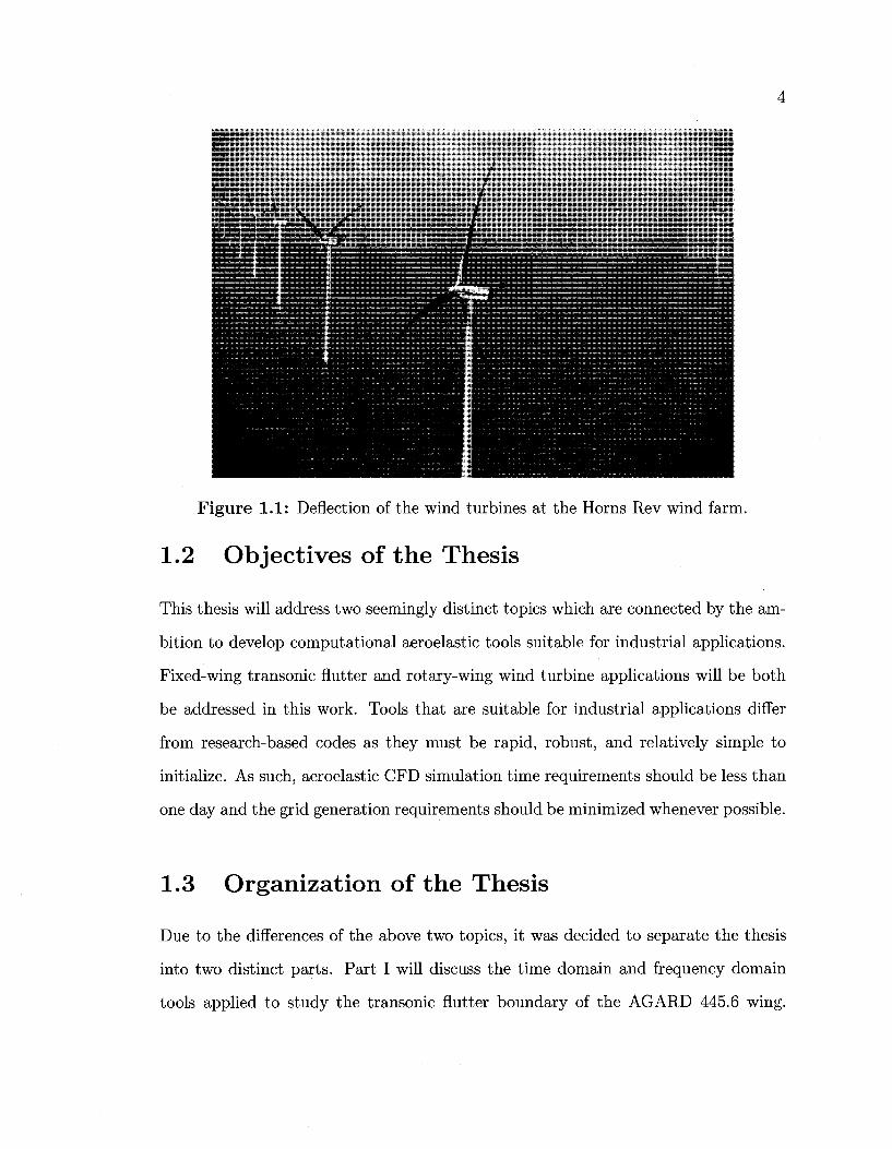
ergy production increases. As the power requirements of wind turbines has continued
to increase, the average wind turbine blade radius has increased substantially from 7
m in 1985 to almost 65 m in 2006. This substantial increase in rotor size is accompa
nied by large blade deflections in nominal operating conditions, as demonstrated in
Figure 1.1 by the offshore turbines at the Horns Rev wind farm in Denmark. Most
of the current aeroelastic wind turbine tools used for commercial and research appli
cations still rely on linear models that assume small blade deflections. However, as
the rotor size of wind turbines continues to increase, there is a need to develop more
accurate structural models that can properly characterize the structural deformation
of large turbines along with the accompanying turbine power output.
The power created by a turbine is also affected by the wake which will reduce the
power generated by downstream turbines in a wind farm. The wake must be properly
characterized in order to analyze the aerodynamic behaviour of turbines in normal
and yawed flow, as well as in wind farms. The work in this thesis uses a nonlinear
structural model coupled with a vortex particle potential flow method developed by
the rotorcraft community and represents one of the few applications of such a model
in the wind turbine field.
4
Figure 1.1: Deflection of the wind turbines at the Horns Rev wind farm.
1.2 Objectives of the Thesis
This thesis will address two seemingly distinct topics which are connected by the am
bition to develop computational aeroelastic tools suitable for industrial applications.
Fixed-wing transonic flutter and rotary-wing wind turbine applications will be both
be addressed in this work. Tools that are suitable for industrial applications differ
from research-based codes as they must be rapid, robust, and relatively simple to
initialize. As such, aeroelastic CFD simulation time requirements should be less than
one day and the grid generation requirements should be minimized whenever possible.
1.3 Organization of the Thesis
Due to the differences of the above two topics, it was decided to separate the thesis
into two distinct parts. Part I will discuss the time domain and frequency domain
tools applied to study the transonic flutter boundary of the AGARD 445.6 wing.
5
The AGARD 445.6 wing was tested to flutter throughout the transonic regime in
the NASA Transonic Dynamics Tunnel in 1963 and has become one of the three
primary benchmark flutter experiments against which numerical codes are validated.
The theory of the correction method developed for frequency domain flutter analysis
along with the results of the aeroelastic time domain simulations have been previ
ously discussed and presented by Beaubien [1]. As this work presents the corrected
frequency domain simulations, the reader is referred to [1,2] for a complete discus
sion of the background, theory, and equations describing both the time domain and
frequency domain simulations. Only the essential theory and background along with
the time domain CFD results and uncorrected frequency domain results from [1] will
be described in this work for completeness.
Part II of the thesis discusses the use of SMARTROTOR, an aeroelastic and aeroa-
coustic analysis tool developed by the rotorcraft community at Carleton University [3],
for studying wind turbine aerodynamics and wake behaviour. The historical devel
opment of wind turbines and a review of the computational techniques developed by
and used by the wind turbine industry will be presented. The computational code
SMARTROTOR is then validated against data from the National Renewable Energy
Laboratory (NREL) full-scale wind turbine experiment. The 10 m diameter stall-
controlled NREL wind turbine was tested in the 24 x 36 m NASA Ames wind tunnel
in 2000 and has become the benchmark experiment for code validation in the wind
turbine industry since the results were published in 2002. Simulations were performed
to assess the code's prediction of power output in unstalled, stalled, and yawed flow
situations. SMARTROTOR's ability to perform wind farm wake interaction studies
is also demonstrated.
Part I
Fixed-wing Aeroelasticity
6
Chapter 2
Time Domain and Frequency Domain
Flut ter Solutions
2.1 Description of Flutter
Aircraft are flexible structures and as such, are susceptible to many aeroelastic phe
nomena including divergence, limit cycle oscillations, and nutter. Divergence is a
static aeroelasticity instability in which aerodynamic loads can deform a wing to fail
ure. Limit cycle oscillations (LCO) are periodic oscillations and can be self-excited or
can be forced by a large disturbance. LCO will cause fatigue problems for certain com
ponents of an aircraft and can affect both passenger comfort and pilot endurance [4].
Flutter however, is an aeroelastic phenomenon that occurs due to undamped oscilla
tions caused by structural and aerodynamic interactions at certain combinations of
air density and freestream velocity. This dynamic instability can occur on control
surfaces, wings, or fuselage sections, and can lead to catastrophic structural failure.
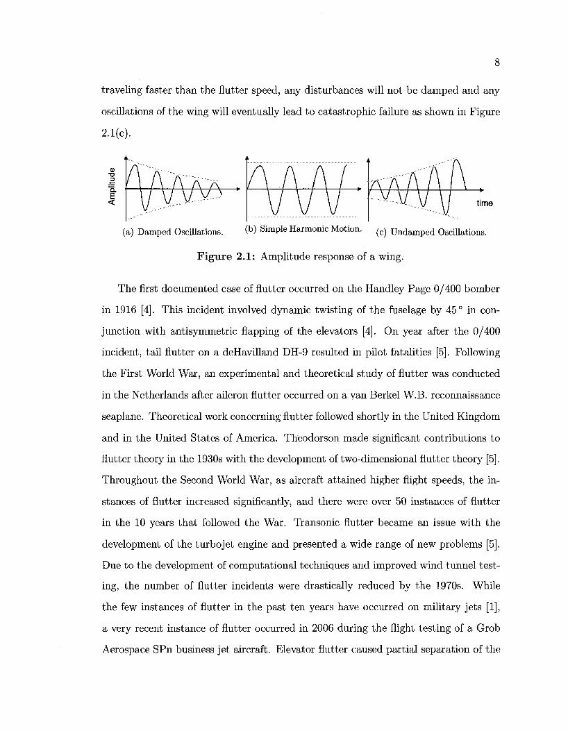
Before the flutter speed is reached, the amplitude of any disturbances to the wing
will be damped as seen in Figure 2.1(a). However, at a speed corresponding to the
flutter boundary of an aircraft at a particular Mach number, the wing motion will
resemble simple harmonic motion as demonstrated in Figure 2.1(b). If an aircraft is
7
8
traveling faster than the nutter speed, any disturbances will not be damped and any
oscillations of the wing will eventually lead to catastrophic failure as shown in Figure
2.1(c).
"O
time
(a) Damped Oscillations. (b) S i m P l e Harmonic Motion. ^ U n d a m p e d Oscillations.
Figure 2.1: Amplitude response of a wing.
The first documented case of flutter occurred on the Handley Page 0/400 bomber
in 1916 [4]. This incident involved dynamic twisting of the fuselage by 45° in con
junction with antisymmetric flapping of the elevators [4]. On year after the 0/400
incident, tail flutter on a deHavilland DH-9 resulted in pilot fatalities [5]. Following
the First World War, an experimental and theoretical study of flutter was conducted
in the Netherlands after aileron flutter occurred on a van Berkel W.B. reconnaissance
seaplane. Theoretical work concerning flutter followed shortly in the United Kingdom
and in the United States of America. Theodorson made significant contributions to
flutter theory in the 1930s with the development of two-dimensional nutter theory [5].
Throughout the Second World War, as aircraft attained higher flight speeds, the in
stances of flutter increased significantly, and there were over 50 instances of flutter
in the 10 years that followed the War. Transonic flutter became an issue with the
development of the turbojet engine and presented a wide range of new problems [5].
Due to the development of computational techniques and improved wind tunnel test
ing, the number of flutter incidents were drastically reduced by the 1970s. While
the few instances of flutter in the past ten years have occurred on military jets [1],
a very recent instance of flutter occurred in 2006 during the flight testing of a Grob
Aerospace SPn business jet aircraft. Elevator flutter caused partial separation of the
9
elevator and horizontal stabilizer and the test aircraft crashed [6]. Though the num
ber of flutter incidents has decreased substantially, all aircraft must be certified for
flutter and other aeroelastic phenomena.
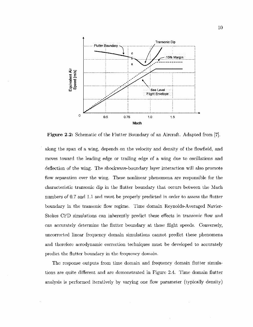
During certification, commercial and military aircraft must demonstrate through
wind tunnel testing, numerical simulations, and flight testing that the aircraft will not
experience flutter within a boundary 15% larger than the flight envelope of the aircraft
[7]. A representative schematic describing the bending-torsion flutter boundary and
the flight envelope of an aircraft can be seen in Figure 2.2. The flutter boundary
defines the speed at which the onset of flutter can occur due to a perturbation of the
wing and aircraft must fly below the flutter speed at all Mach numbers. The regions
of the flight envelope where the damped, harmonic, and undamped motions presented
above in Figure 2.1 will occur are indicated in Figure 2.2 by the letters a, b, and c,
respectively. The most critical region of the flutter boundary is characterized by the
transonic dip and typically occurs between a Mach number of 0.9 and 1.1. After a
Mach number of 1.2, the flutter speed rises due to the rearward shift in the centre of
pressure on the surface of the wing and is typically not a concern. However, in the
most critical region between Mach numbers of 0.9 and 1.1, nonlinear transonic effects
are present over the wing and control surfaces of aircraft that cannot be properly
captured by linear solution techniques.
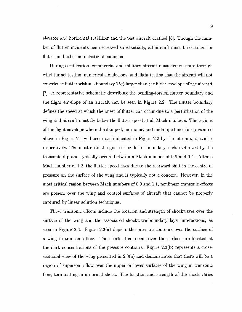
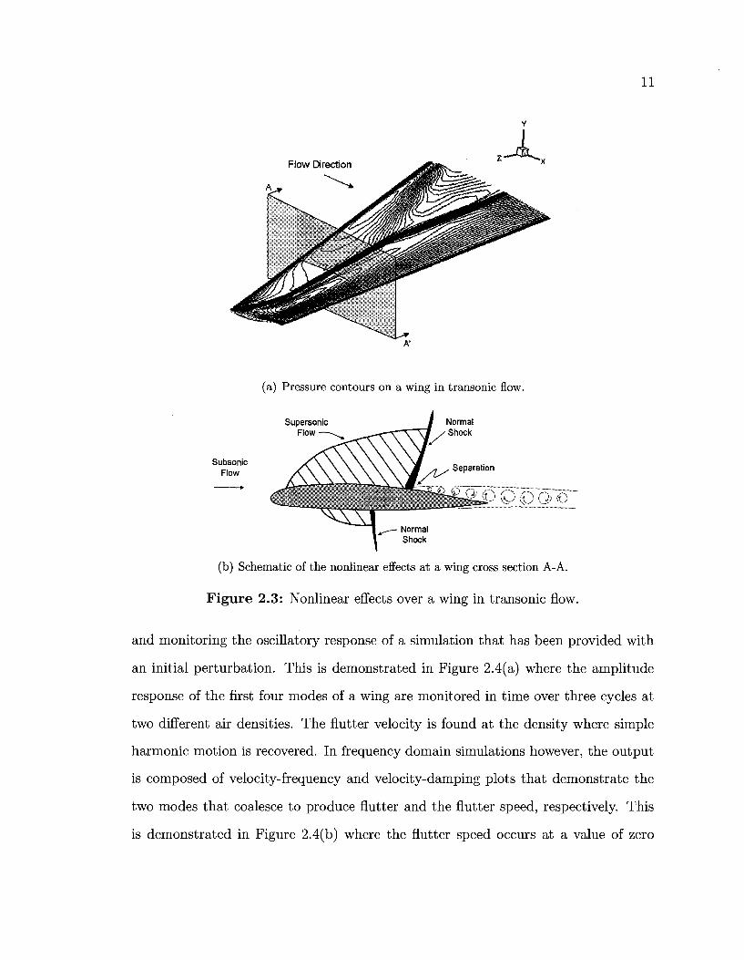
These transonic effects include the location and strength of Shockwaves over the
surface of the wing and the associated shockwave-boundary layer interactions, as
seen in Figure 2.3. Figure 2.3(a) depicts the pressure contours over the surface of
a wing in transonic flow. The shocks that occur over the surface are located at
the dark concentrations of the pressure contours. Figure 2.3(b) represents a cross-
sectional view of the wing presented in 2.3(a) and demonstrates that there will be a
region of supersonic flow over the upper or lower surfaces of the wing in transonic
flow, terminating in a normal shock. The location and strength of the shock varies
10
< IF
(15 •—'
! " § .2 a) S- e'er yi 111 "*
u 0.5 0.75 1.0 1.5
Mach
Figure 2.2: Schematic of the Flutter Boundary of an Aircraft. Adapted from [7].
along the span of a wing, depends on the velocity and density of the flowfield, and
moves toward the leading edge or trailing edge of a wing due to oscillations and
deflection of the wing. The shockwave-boundary layer interaction will also promote
flow separation over the wing. These nonlinear phenomena are responsible for the
characteristic transonic dip in the nutter boundary that occurs between the Mach
numbers of 0.7 and 1.1 and must be properly predicted in order to assess the nutter
boundary in the transonic flow regime. Time domain Reynolds-Averaged Navier-
Stokes CFD simulations can inherently predict these effects in transonic flow and
can accurately determine the flutter boundary at these flight speeds. Conversely,
uncorrected linear frequency domain simulations cannot predict these phenomena
and therefore aerodynamic correction techniques must be developed to accurately
predict the flutter boundary in the frequency domain.
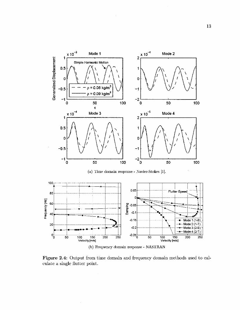
The response outputs from time domain and frequency domain flutter simula
tions are quite different and are demonstrated in Figure 2.4. Time domain flutter
analysis is performed iteratively by varying one flow parameter (typically density)
Transonic Dip
11
Flow Direction
(a) Pressure contours on a wing in transonic flow.
Supersonic Flow
Normal Shock
Subsonic Flow
(b) Schematic of the nonlinear effects at a wing cross section A-A.
Figure 2.3: Nonlinear effects over a wing in transonic flow.
and monitoring the oscillatory response of a simulation that has been provided with
an initial perturbation. This is demonstrated in Figure 2.4(a) where the amplitude
response of the first four modes of a wing are monitored in time over three cycles at
two different air densities. The flutter velocity is found at the density where simple
harmonic motion is recovered. In frequency domain simulations however, the output
is composed of velocity-frequency and velocity-damping plots that demonstrate the
two modes that coalesce to produce flutter and the flutter speed, respectively. This
is demonstrated in Figure 2.4(b) where the flutter speed occurs at a value of zero
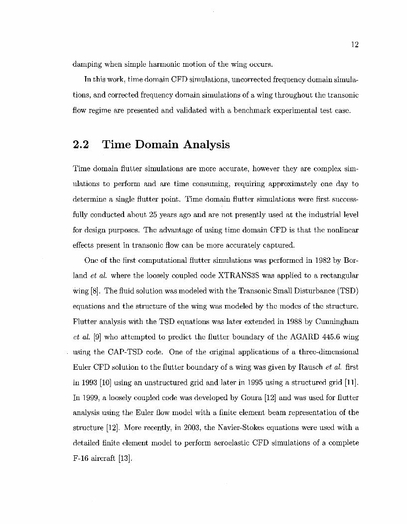
12
damping when simple harmonic motion of the wing occurs.
In this work, time domain CFD simulations, uncorrected frequency domain simula
tions, and corrected frequency domain simulations of a wing throughout the transonic
flow regime are presented and validated with a benchmark experimental test case.
2.2 Time Domain Analysis
Time domain flutter simulations are more accurate, however they are complex sim
ulations to perform and are time consuming, requiring approximately one day to
determine a single flutter point. Time domain nutter simulations were first success
fully conducted about 25 years ago and are not presently used at the industrial level
for design purposes. The advantage of using time domain CFD is that the nonlinear
effects present in transonic flow can be more accurately captured.
One of the first computational flutter simulations was performed in 1982 by Bor
land et al. where the loosely coupled code XTRANS3S was applied to a rectangular
wing [8]. The fluid solution was modeled with the Transonic Small Disturbance (TSD)
equations and the structure of the wing was modeled by the modes of the structure.
Flutter analysis with the TSD equations was later extended in 1988 by Cunningham
et al. [9] who attempted to predict the flutter boundary of the AGARD 445.6 wing
using the CAP-TSD code. One of the original applications of a three-dimensional
Euler CFD solution to the flutter boundary of a wing was given by Rausch et al. first
in 1993 [10] using an unstructured grid and later in 1995 using a structured grid [11].
In 1999, a loosely coupled code was developed by Goura [12] and was used for flutter
analysis using the Euler flow model with a finite element beam representation of the
structure [12]. More recently, in 2003, the Navier-Stokes equations were used with a
detailed finite element model to perform aeroelastic CFD simulations of a complete
F-16 aircraft [13].
13
x10 Mode 1 x10 Mode 2
100
50 100 0 50
(a) Time domain response - Navier-Stokes [1].
100
100
80
60
40
20-
» 1 • * — i A — i U
T i 4 4 1 — • — f
50 100 150 Velocity [m/s]
200 250
0.05
-0.05
-0.1
-0.15
-0.2
-0.25
Flutter Speed t i
- { i V-j -»-Mode1(1-B) --»-Mode2(1-T) —»-Mode3(2-B)--*-Mode4(2-T)
50 100 150 Velocity [m/s]
200 250
(b) Frequency domain response - NASTRAN
Figure 2.4: Output from time domain and frequency domain methods used to calculate a single nutter point.
14
In the current work, the time domain flutter simulations were conducted using
both Euler and Navier-Stokes representations [1] and will serve as the benchmark
case for the corrected frequency domain technique, along with the experimental results
from the AGARD 445.6 wind tunnel test.
Time Domain Aerodynamic Model
The time domain flutter simulations were performed with the Carleton Multi-Block
(CMB) Computational Fluid Dynamics code which is based on a code originally
developed at the University of Glasgow [14] and further extended at Carleton Uni
versity. CMB has a proven capability of capturing transonic effects [12,14]. It is a
three-dimensional CFD code that uses a cell-centred finite volume technique to solve
either the Euler or the Reynolds Averaged Navier-Stokes (RANS) equations. The
diffusive terms are discretized with a central differencing scheme and the convective
terms are solved using an approximate Riemann solver that applies either Roe's or
Osher's scheme. Osher's upwind scheme was used in all of the simulations performed
as part of this study. Second order spatial accuracy is achieved with MUSCL variable
extrapolation with a Van Albada limiter to prevent dispersion near Shockwaves [1].
The boundary conditions are dealt with using two layers of ghost cells that lie
outside the domain. The far field boundary condition is met by setting the ghost cell
values equal to the freestream values. For viscous flows, no-slip is imposed at the wall
and for inviscid flows, the normal velocity on any solid surfaces is set to zero.
Steady flow simulations begin with an explicit scheme to smooth out the flow
solution, which then switches to an implicit scheme for more rapid convergence. Pre
conditioning is based on block incomplete lower-upper surface factorization and is
decoupled between blocks to increase the parallel performance of the solver [15]. In
unsteady flows, the multigrid dual-time method of Jameson is used to obtain sec
ond order accuracy in time. In the Jameson dual-time method, equations are solved
15
implicitly in both pseudo-time and real-time.
Turbulence modeling in CMB can be performed using a variety of models, includ
ing the Spalart-Allmaras, k-e, k-u;, and Shear Stress Transport (SST) models. The
two-equation baseline SST model was selected for this study because of its appli
cability to simulations with complex surface interactions and based on other tests
performed with CMB [16]. The SST model blends the k-e model (which is generally
robust outside the boundary layer) with the k-cu model (which is more robust within
the boundary layer). A complete description of the SST model that was implemented
in this study can be found in [1,16].
Time Domain Structural Model
In order to accurately model aeroelastic problems, the geometry of the wing and the
aerodynamic mesh must both deform during simulations. The static and dynamic
response of the structure is resolved using a finite element method linear beam model.
The mass ([M]) and stiffness ([K]) matrices of an elastic wing are related to external
forces {{fs}) according to Equation 2.1
[M]{u} + [K]{u} = {fs} (2.1)
The mass and stiffness matrices in the linear structural system were determined a
priori with MSC/NASTRAN.
The structural displacements are written as a linear combination of the generalized
coordinates ({q}) and the physical displacements of the structure ({«}) according to
Equation 2.2 [1]
{«} = [$] {q} (2.2)
where [$] is the modal transformation matrix. The eigenvalues of the system are
16
solved and scaled according to Equation 2.3.
[$]T [M] [$] = 1 (2.3)
The finite element method equations can then be described by Equation 2.4.
*M+u?{q} = [*]T{fs} (2.4)
Equation 2.4 is solved using a two-step Runge-Kutta method and is iterated in pseudo
time along with the aerodynamic solution to avoid time sequencing errors from the
dual-time approach [17].
For aeroelastic simulations, the deformation of the computational domain is ac
complished by interpolating the wing surface displacements to the interior nodes. The
deformation of the aerodynamic mesh is determined in conjunction with the structural
beam model deflection using Transfinite Interpolation of Displacements (TFI) within
all of the blocks containing a wing surface [17]. The wing surface deflections (xajk)
are interpolated to the grid points within the domain (xijk) according to Equation
2.5.
SXijk = rfx^ik (2.5)
The term <£>° in Equation 2.5 represents a blending function which varies between one
at the wing surface and zero at the opposite face of the block containing the wing
surface. The cell volumes are recalculated using a Global Conservation Law (GCL) by
considering volume fluxes through the cell faces. The deflections of the wing surface
ixa,ik) a r e obtained from the transformation of the structural grid deflections [1].
As the structural and aerodynamic meshes are not coincident in this type of
analysis, coupling between the structural and aerodynamic models is achieved using
the Constant Volume Tetrahedron (CVT) scheme [17].
17
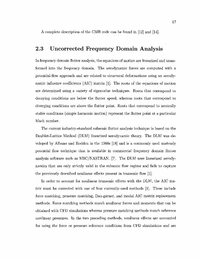
A complete description of the CMB code can be found in [12] and [14].
2.3 Uncorrected Frequency Domain Analysis
In frequency domain flutter analysis, the equations of motion are linearized and trans
formed into the frequency domain. The aerodynamic forces are computed with a
potential-flow approach and are related to structural deformations using an aerody
namic influence coefficients (AIC) matrix [1]. The roots of the equations of motion
are determined using a variety of eigenvalue techniques. Roots that correspond to
decaying conditions are below the flutter speed, whereas roots that correspond to
diverging conditions are above the flutter point. Roots that correspond to neutrally
stable conditions (simple harmonic motion) represent the flutter point at a particular
Mach number.
The current industry-standard subsonic flutter analysis technique is based on the
Doublet-Lattice Method (DLM) linearized aerodynamic theory. The DLM was de
veloped by Albano and Rodden in the 1960s [18] and is a commonly used unsteady
potential flow technique that is available in commercial frequency domain flutter
analysis software such as MSC/NASTRAN. [7]. The DLM uses linearized aerody
namics that are only strictly valid in the subsonic flow regime and fails to capture
the previously described nonlinear effects present in transonic flow [1].
In order to account for nonlinear transonic effects with the DLM, the AIC ma
trix must be corrected with one of four currently-used methods [1]. These include
force matching, pressure matching, Dau-garner, and modal AIC matrix replacement
methods. Force matching methods match nonlinear forces and moments that can be
obtained with CFD simulations whereas pressure matching methods match reference
nonlinear pressures. In the two preceding methods, nonlinear effects are accounted
for using the force or pressure reference conditions from CFD simulations and are
18
incorporated into a corrected AIC matrix. Dau-garner methods use steady nonlin
ear data and semi-empirical relationships to determine corrected nonlinear pressures.
The modal AIC method however, creates a new nonlinear AIC matrix that is based
on the modal displacement of a wing [1].
The current frequency domain method uses the pressure matching method devel
oped by Reference [19] to correct the AIC matrix and will be presented in Section
2.4. A thorough discussion of the above-mentioned correction methods can be found
in [1,19]-
The uncorrected aerodynamic modeling with the DLM and the representation of
the aeroelastic system of equations in the frequency domain will be briefly presented
in the following Section, but a more detailed derivation of the relevant equations and
a description of the interconnection of the structure with the system aerodynamics is
given by Beaubien [1]. The derivation of the selected correction method to account
for nonlinear aerodynamics in the frequency domain is then presented.
2.3.1 Aerodynamic Modeling
Lifting surface theory is used to solve the unsteady compressible flow over a wing using
the Doublet Lattice Method (DLM) assuming that the flow is inviscid, isentropic,
subsonic, and fully attached. The thickness of the lifting surface is neglected and
small-perturbation theory is used assuming that changes in the angle of attack will be
small. Compressibility is taken into account using the Prandtl-Glauert formula [20].
The DLM is based on a panel method approach and is widely used in industry.
While the following is an introduction to the DLM, a detailed derivation can be
found in [21,18].
The linearized oscillatory subsonic lifting surface theory relates the normal velocity
(W) at the lifting surface to the pressure coefficient difference over the surface (ACp),
19
which are both defined in Equations 2.6 and 2.7.
W = C/ooRe (we™*) (2.6)
AP = i/zpU^Re (ACpe**) (2.7)
The normal velocity and pressure difference can be related by an integral equation
written in the reduced frequency domain, as described by Equation 2.8
w(x,y,z) = — K(x-£,y-r],z-(,k, M^ACpd^da (2.8)
where r\ is the streamwise coordinate, a is the tangential spanwise coordinate,
k = wbg/Uoo is the reduced frequency, u is the oscillation frequency, bs is the root
semi-chord, and C/QO is the freestream velocity. The kernel K in Equation 2.8 is the
downwash at a point (x, y, z) induced by a doublet of unit strength located at (£, 77, £)
in elemental coordinates [22]. The lifting surface is divided into a grid of trapezoidal
elements over which the pressure is constant [1]. The double integral over one ele
ment can be performed in the £ and fj directions. The integration in the streamwise
£ direction by concentrating the integrand at the quarter-chord point of a panel, 771/4
and Equation 2.8 can be rewritten as
w (x,y,z) = ^2&CP-^- K(x-^1/4,y-fj,z,k,M00)dfi (2.9)
where e is the semi-width of a lifting panel. The downwash boundary condition in
Equation 2.9 is known and the pressure difference coefficient over each element is
unknown. If the downwash can be satisfied for each element in the lifting surface,
20
Equation 2.9 can be written in matrix form as Equation 2.10.
{w} = [D]{ACP} (2.10)
Each element in [D] is a downwash factor Dij at the location x^y^Zi caused by-
element j as seen in Equation 2.10.
D^ = — - / K(xi- 6/4, Vi - fj, Zi, k, M^dfj (2.11) —^j
The downwash factor D^ can be separated into a steady and unsteady part and the
solution must satisfy both the Kutta condition and the flow tangency condition. The
Kutta condition states that the pressure difference at the trailing edge of a thin lifting
surface must be zero and the flow tangency condition states that the velocity vector
at a surface must be tangent to the surface of a lifting body in inviscid flow [23]. The
flow tangency condition is satisfied at the control and receiving point found on each
element. The downwash collocation control point is centred along the three-quarter
chord line of each element [1].
The pressure distribution in Equation 2.10 can be obtained by multiplying the
inverse of the downwash factor matrix [D] by the downwash vector {w}. The inverse
of [D] is the AIC matrix and can be related to the pressure coefficient as a function
of reduced frequency according to Equation 2.12. The coefficients of the AIC matrix
represent rates of the pressure variation caused by a particular displacement ampli
tude input [1]. The downwash vector in Equation 2.12 is related to the amplitude of
the pitch and plunge motions at each panel.
{ACp(ik)} = [AIC(ik)] {w(ik)} (2.12)
Once the pressure coefficients have been determined, the aerodynamic loading vector
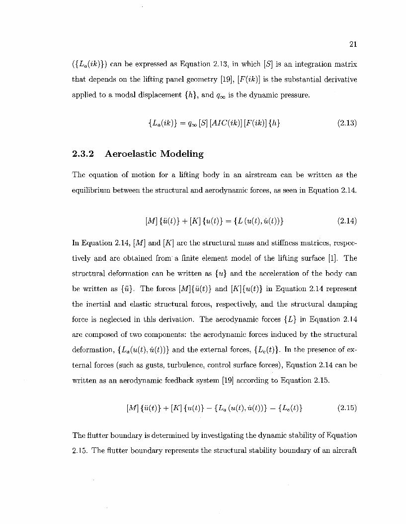
21
({La(ik)}) can be expressed as Equation 2.13, in which [S] is an integration matrix
that depends on the lifting panel geometry [19], [^(iA;)] is the substantial derivative
applied to a modal displacement {h}, and g<x, is the dynamic pressure.
{La(ik)} = goo [S] [AIC{ik)\ [F{ik)\ {h} (2.13)
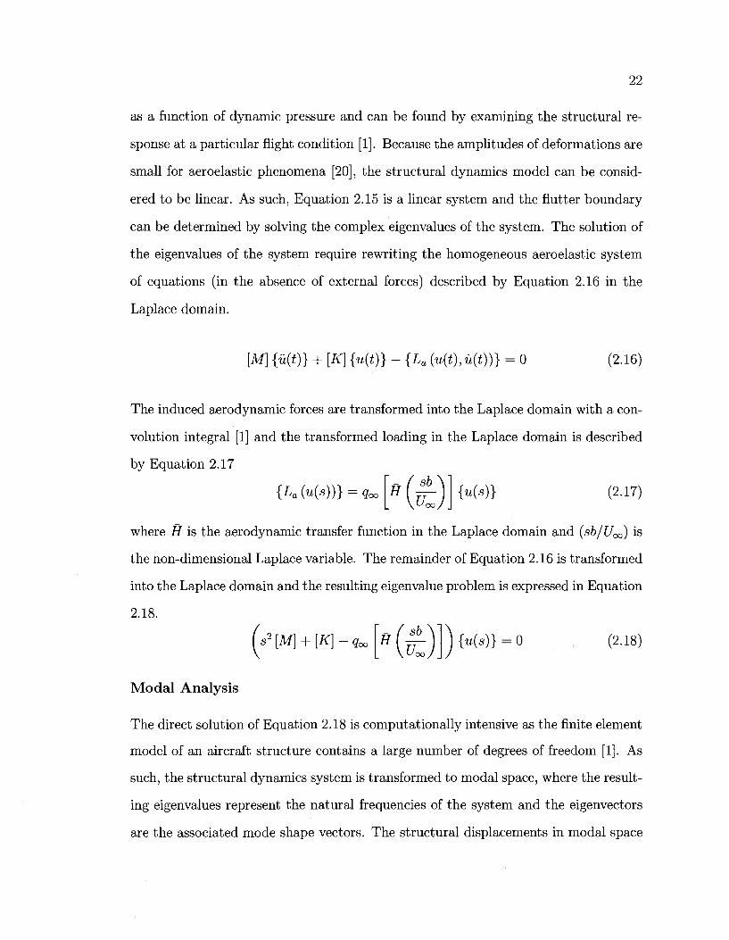
2.3.2 Aeroelastic Modeling
The equation of motion for a lifting body in an airstream can be written as the
equilibrium between the structural and aerodynamic forces, as seen in Equation 2.14.
[M] {«(*)} + [K] {«(*)} = {L («(*),«(*))} (2.14)
In Equation 2.14, [M] and [K] are the structural mass and stiffness matrices, respec
tively and are obtained from a finite element model of the lifting surface [1]. The
structural deformation can be written as {u} and the acceleration of the body can
be written as {u}. The forces [M]{ii(t)} and [if] {«(£)} in Equation 2.14 represent
the inertial and elastic structural forces, respectively, and the structural damping
force is neglected in this derivation. The aerodynamic forces {L} in Equation 2.14
are composed of two components: the aerodynamic forces induced by the structural
deformation, {La(u(t), u(t))} and the external forces, {Le(t)}. In the presence of ex
ternal forces (such as gusts, turbulence, control surface forces), Equation 2.14 can be
written as an aerodynamic feedback system [19] according to Equation 2.15.
[M] {«(*)} + [K] {u{t)} - {La (u(t),ii(t))} = {Le(t)} (2.15)
The flutter boundary is determined by investigating the dynamic stability of Equation
2.15. The flutter boundary represents the structural stability boundary of an aircraft
22
as a function of dynamic pressure and can be found by examining the structural re
sponse at a particular flight condition [1]. Because the amplitudes of deformations are
small for aeroelastic phenomena [20], the structural dynamics model can be consid
ered to be linear. As such, Equation 2.15 is a linear system and the flutter boundary
can be determined by solving the complex eigenvalues of the system. The solution of
the eigenvalues of the system require rewriting the homogeneous aeroelastic system
of equations (in the absence of external forces) described by Equation 2.16 in the
Laplace domain.
[M] {il(t)} + [K] {u(t)} - {La (u(t), u(t))} = 0 (2.16)
The induced aerodynamic forces are transformed into the Laplace domain with a con
volution integral [1] and the transformed loading in the Laplace domain is described
by Equation 2.17
{La (u(s))} = q0 n(it {u(s)} (2.17)
where H is the aerodynamic transfer function in the Laplace domain and (sb/Uoo) is
the non-dimensional Laplace variable. The remainder of Equation 2.16 is transformed
into the Laplace domain and the resulting eigenvalue problem is expressed in Equation
2.18.
( > [M] + [K] - Qoo \S (A) j) {u{s)} = o (2.18)
Modal Analysis
The direct solution of Equation 2.18 is computationally intensive as the finite element
model of an aircraft structure contains a large number of degrees of freedom [1]. As
such, the structural dynamics system is transformed to modal space, where the result
ing eigenvalues represent the natural frequencies of the system and the eigenvectors
are the associated mode shape vectors. The structural displacements in modal space
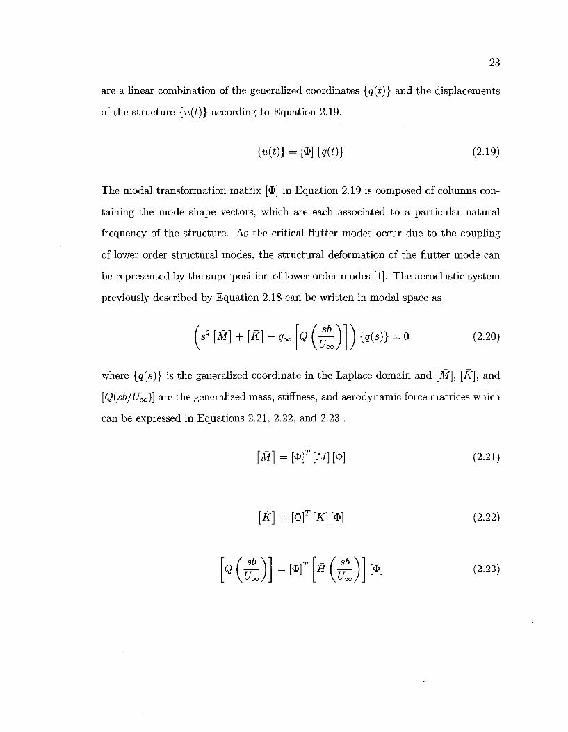
23
are a linear combination of the generalized coordinates {q(t)} and the displacements
of the structure {u(t)} according to Equation 2.19.
M*)} = [*] {«(*)} (2-19)
The modal transformation matrix [<&] in Equation 2.19 is composed of columns con
taining the mode shape vectors, which are each associated to a particular natural
frequency of the structure. As the critical flutter modes occur due to the coupling
of lower order structural modes, the structural deformation of the flutter mode can
be represented by the superposition of lower order modes [1]. The aeroelastic system
previously described by Equation 2.18 can be written in modal space as
( > [M] + [K] - q(
where {q(s)} is the generalized coordinate in the Laplace domain and [M], [K], and
[(^(sb/Uoo)] are the generalized mass, stiffness, and aerodynamic force matrices which
can be expressed in Equations 2.21, 2.22, and 2.23 .
[M] = [$]T [M] [$] (2.21)
[K] = mT [K] [<*>] (2.22)
[<)HT
< {«(*)} = o (2.20)
H sb_
[*] (2.23)
24
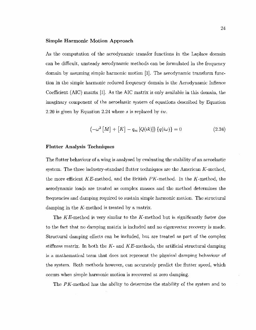
Simple Harmonic Motion Approach
As the computation of the aerodynamic transfer functions in the Laplace domain
can be difficult, unsteady aerodynamic methods can be formulated in the frequency
domain by assuming simple harmonic motion [1]. The aerodynamic transform func
tion in the simple harmonic reduced frequency domain is the Aerodynamic Inflence
Coefficient (AIC) matrix [1]. As the AIC matrix is only available in this domain, the
imaginary component of the aeroelastic system of equations described by Equation
2.20 is given by Equation 2.24 where s is replaced by iw.
(-u2 [M] + [K] - <7oo [Q(ik)]) {q{iuj)} = 0 (2.24)
Flutter Analysis Techniques
The flutter behaviour of a wing is analysed by evaluating the stability of an aeroelastic
system. The three industry-standard flutter techniques are the American K-method,
the more efficient KE-m.eih.od, and the British Pif-method. In the if-method, the
aerodynamic loads are treated as complex masses and the method determines the
frequencies and damping required to sustain simple harmonic motion. The structural
damping in the X-method is treated by a matrix.
The KE-method is very similar to the if-method but is significantly faster due
to the fact that no damping matrix is included and no eigenvector recovery is made.
Structural damping effects can be included, but are treated as part of the complex
stiffness matrix. In both the K- and KE-va.eth.ods, the artificial structural damping
is a mathematical term that does not represent the physical damping behaviour of
the system. Both methods however, can accurately predict the flutter speed, which
occurs when simple harmonic motion is recovered at zero damping.
The Pif-method has the ability to determine the stability of the system and to
25
estimate the physical damping of the system at subcritical speeds (at speeds below
the flutter boundary). The aerodynamic matrices are treated as frequency dependent
springs and dampers in the PK-method.
The frequency domain flutter analysis was performed using MSC/NASTRAN and
KEDLMPL. MSC/NASTRAN is an industry-standard finite element package that
can perform K, KE, and PK flutter analyses. The software was rewritten in 2001,
and as such, the aerodynamic matrices are no longer accessible for interpretation or
correction [1]. The second software package that was used is KEDLMPL, a frequency
domain flutter analysis tool designed at the Instituto de Aeronautica e Espac,o in
Brazil [19]. As the source code for KEDLMPL was generously provided, the aerody
namic matrices were accessible, and aerodynamic corrections could be implemented
and evaluated. As KEDLMPL was designed specifically to perform i^jB-flutter anal
ysis for wings, all of the frequency domain flutter analyses with KEDLMPL and
MSC/NASTRAN were performed with the KE-m.eih.od for consistency between fre
quency domain results.
2.4 Corrected Frequency Domain Analysis
A procedure was developed to correct the frequency domain flutter boundary pro
duced with KEDLMPL to account for nonlinear aerodynamics in the transonic
regime [1]. The technique corrects the Aerodynamic Influence Coefficients (AIC)
matrix used within the DLM solver. A pressure matching method was applied that
involved a downwash weighting approach using unsteady nonlinear pressure coeffi
cients obtained from time domain CFD simulations [1,19]. The relationship between
the AIC matrix, the downwash vector (w), and the pressure difference coefficient
vector (ACp) is described in Equation 2.25 as a function of reduced frequency. The
uncorrected AIC matrix is computed within the DLM and relates the lifting pressures
26
to a given displacement input and is independent of the vibration modes.
{ACP(ik)} = [AIC{ik)\ {w(ik)} (2.25)
The nonlinear unsteady lifting pressures are obtained by performing unsteady rigid
body pitching motions with CFD. Based on the work of [19], a harmonic pitching
motion about the root midchord was simulated in CMB according to Equation 2.26
a (t) = am + Aa sin (2krt) (2.26)
where the mean angle of attack (am) was 0°, the amplitude of the oscillation (Aa)
was 1 °, and kr represents the reduced frequency of the oscillatory motion. The
parameters used for the unsteady pitching motion were based on the experiences of
Silva [19]. Following the harmonic pitching simulation, the pressures obtained on the
upper and lower surface of the wing over one complete pitching cycle are subtracted
to obtain the nonlinear ACP vector, as described in Equation 2.27
{AC?L} = CLP
OWER - CU/PER (2.27)
As the AIC correction procedure is implemented in the frequency domain, the ACp
vector described in Equation 2.27 must be Fourier transformed to obtain the fre
quency domain representation of the unsteady lifting pressures. The first harmonic
of the unsteady pressure coefficients was obtained using the discrete Fourier transform
(DFT) described by Equations 2.28 and 2.29 [24,19] .
h MA m i + T " T
R e ( 0 ~ Y CPsm(krmAr) (2.28) mi
27
Im(C^ L ) = ^ ^ ^ CPcos(A;rmAr) (2.29) mi
where m is the time step number, M is the Mach number of the unsteady simulation,
and A T is the non-dimensional time step. A complete derivation of the DFT can be
found in Appendix A.
The nonlinear lifting pressure vector is then written in complex notation according
to Equation 2.30 prior to its implementation.
{AC£L} = (Re {AC$L(ik)} + Im {AC$L(ik)}) (2.30)
In order to account for nonlinear aerodynamics in the AIC matrix, Equation 2.25
is modified to include a nonlinear weighting matrix [WT], as seen in Equation 2.31.
The normalized downwash vector term ( w a) in Equation 2.31 is normalized by the
amplitude of the unsteady pitching motion as described in Equation 2.32 [19].
{AC$L} = [AIC{ik)\ [WT{ik)\ {wa(ik)} (2.31)
{w«m={^ (2.32)
Prior to solving the weighting matrix, a nonlinear downwash term must be calculated
based on the nonlinear lifting pressures. The nonlinear downwash equation is obtained
by multiplying the Fourier transformed nonlinear pressures from the unsteady rigid
body CFD simulation with the AIC matrix by rearranging Equation 2.25 below.
{wNL(ik)} = [AIC{ik)Yl {AC$L} (2.33)
The nonlinear downwash vector is then divided by the normalized downwash vector
28
from Equation 2.32 to produce the nonlinear weighting matrix [WT], as seen in
Equation 2.34 [19].
[WT{ik)\ = {fL^} (2.34) 1 v n {wa(ik)} v '
Once the weighting matrix has been determined, the nonlinear aerodynamic loads can
be calculated using Equation 2.35, where q^ is the dynamic pressure and [S] is an
integration matrix constructed from the geometric characteristics of the lifting panel
[1]. The nonlinear aerodynamic loads (L^L) are used in the frequency domain solver
in order to calculate the corrected frequency domain flutter boundary. Additional
information regarding the AIC correction procedure can be found in Reference [19].
La = qoo[S][AIC(ik)}[WT(ik)}{w{ik)} (2.35)
Chapter 3
Flutter Simulation Results
Simulation results with the time domain, uncorrected frequency domain, and cor
rected frequency domain methods described in the previous chapter will be presented.
The three sets of results will be compared to the benchmark experimental test case
available for transonic flutter, the AGARD 445.6 wing. The chapter begins with
a description of the experimental setup followed by the time domain, uncorrected
frequency domain, and corrected frequency domain results. The time domain and
uncorrected frequency domain results obtained by Beaubien are presented below for
completeness [1].
3.1 AGARD 445.6 Test Case
The AGARD 445.6 experimental test case is one of the three primary transonic flut
ter experiments. The tests were performed in 1963 at the NASA Langley Transonic
Dynamics Tunnel and involved the destruction of a transonic wing geometry under
flutter conditions throughout the transonic regime [25]. This test case has since be
come the benchmark for numerical transonic flutter simulations. The wing model had
a NACA 65A004 airfoil, an aspect ratio of 4, a leading edge sweep angle of 45°, a
29
30
taper ratio of 0.66, and a root chord of 0.58 m. A complete description of the exper
imental setup can be found in [25]. The laminated mahogany experimental model,
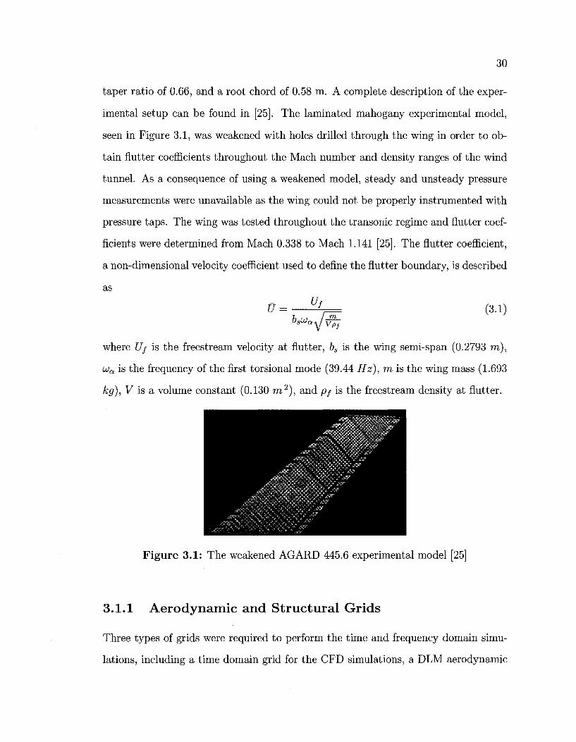
seen in Figure 3.1, was weakened with holes drilled through the wing in order to ob
tain flutter coefficients throughout the Mach number and density ranges of the wind
tunnel. As a consequence of using a weakened model, steady and unsteady pressure
measurements were unavailable as the wing could not be properly instrumented with
pressure taps. The wing was tested throughout the transonic regime and flutter coef
ficients were determined from Mach 0.338 to Mach 1.141 [25]. The flutter coefficient,
a non-dimensional velocity coefficient used to define the flutter boundary, is described
as
0 = —U~W (") bsUJa\jVp~f
where Uf is the freestream velocity at flutter, bs is the wing semi-span (0.2793 m),
u>a is the frequency of the first torsional mode (39.44 Hz), m is the wing mass (1.693
kg), V is a volume constant (0.130 m2), and pf is the freestream density at flutter.
Figure 3.1: The weakened AGARD 445.6 experimental model [25]
3.1.1 Aerodynamic and Structural Grids
Three types of grids were required to perform the time and frequency domain simu
lations, including a time domain grid for the CFD simulations, a DLM aerodynamic
31
mesh for the frequency domain solvers, and a structural model for the frequency
domain simulations. The mode shapes obtained from the structural model are also
input into the integrated beam model for the aeroelastic time domain simulations
performed in CMB.
Time Domain CFD Mesh
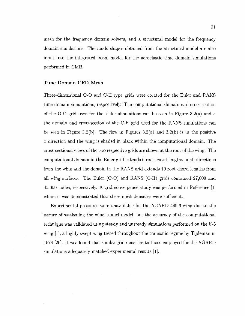
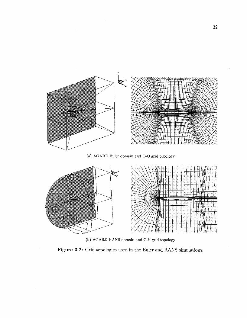
Three-dimensional 0 - 0 and C-H type grids were created for the Euler and RANS
time domain simulations, respectively. The computational domain and cross-section
of the 0 - 0 grid used for the Euler simulations can be seen in Figure 3.2(a) and a
the domain and cross-section of the C-H grid used for the RANS simulations can
be seen in Figure 3.2(b). The flow in Figures 3.2(a) and 3.2(b) is in the positive
x direction and the wing is shaded in black within the computational domain. The
cross-sectional views of the two respective grids are shown at the root of the wing. The
computational domain in the Euler grid extends 6 root chord lengths in all directions
from the wing and the domain in the RANS grid extends 10 root chord lengths from
all wing surfaces. The Euler (0-0) and RANS (C-H) grids contained 27,000 and
45,000 nodes, respectively. A grid convergence study was performed in Reference [1]
where it was demonstrated that these mesh densities were sufficient.
Experimental pressures were unavailable for the AGARD 445.6 wing due to the
nature of weakening the wind tunnel model, but the accuracy of the computational
technique was validated using steady and unsteady simulations performed on the F-5
wing [1], a highly swept wing tested throughout the transonic regime by Tijdeman in
1978 [26]. It was found that similar grid densities to those employed for the AGARD
simulations adequately matched experimental results [1].
32
(a) AGARD Euler domain and O-O grid topology
(b) AGARD RANS domain and C-H grid topology
Figure 3.2: Grid topologies used in the Euler and RANS simulations.
33
Structural Model
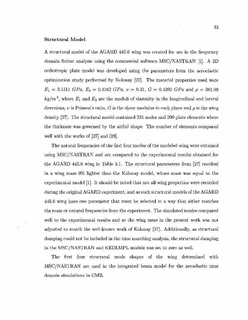
A structural model of the AGARD 445.6 wing was created for use in the frequency
domain flutter analysis using the commercial software MSC/NASTRAN [1]. A 2D
orthotropic plate model was developed using the parameters from the aeroelastic
optimization study performed by Kolonay [27]. The material properties used were
Ex = 3.1511 GPa, E2 = 0.4162 GPa, v = 0.31, G = 0.4392 GPa and p = 381.98
kg/m3, where E\ and E2 are the moduli of elasticity in the longitudinal and lateral
directions, v is Poisson's ratio, G is the shear modulus in each plane and p is the wing
density [27]. The structural model contained 231 nodes and 200 plate elements where
the thickness was governed by the airfoil shape. The number of elements compared
well with the works of [27] and [19].
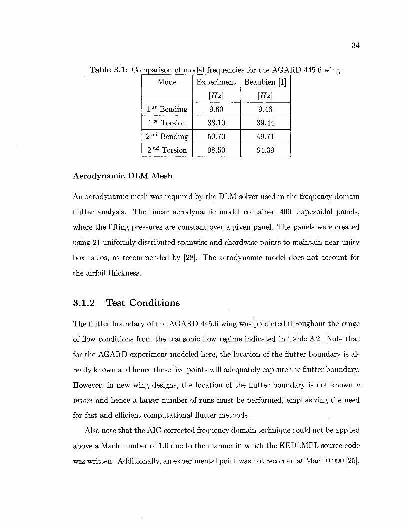
The natural frequencies of the first four modes of the modeled wing were obtained
using MSC/NASTRAN and are compared to the experimental results obtained for
the AGARD 445.6 wing in Table 3.1. The structural parameters from [27] resulted
in a wing mass 9% lighter than the Kolonay model, whose mass was equal to the
experimental model [1]. It should be noted that not all wing properties were recorded
during the original AGARD experiment, and as such structural models of the AGARD
445.6 wing have one parameter that must be selected in a way that either matches
the mass or natural frequencies from the experiment. The simulated modes compared
well to the experimental results and so the wing mass in the present work was not
adjusted to match the well-known work of Kolonay [27]. Additionally, as structural
damping could not be included in the time marching analysis, the structural damping
in the MSC/NASTRAN and KEDLMPL models was set to zero as well.
The first four structural mode shapes of the wing determined with
MSC/NASTRAN are used in the integrated beam model for the aeroelastic time
domain simulations in CMB.
34
Table 3.1: Comparison of modal frequencies for the AGARD 445.6 wing
Mode
1st Bending
1st Torsion
2nd Bending
2 nd Torsion
Experiment
[Hz]
9.60
38.10
50.70
98.50
Beaubien [1]
[Hz]
9.46
39.44
49.71
94.39
Aerodynamic DLM Mesh
An aerodynamic mesh was required by the DLM solver used in the frequency domain
flutter analysis. The linear aerodynamic model contained 400 trapezoidal panels,
where the lifting pressures are constant over a given panel. The panels were created
using 21 uniformly distributed spanwise and chord wise points to maintain near-unity
box ratios, as recommended by [28]. The aerodynamic model does not account for
the airfoil thickness.
3.1.2 Test Conditions
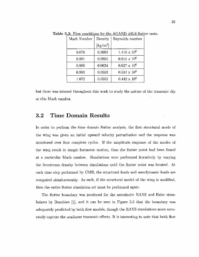
The flutter boundary of the AGARD 445.6 wing was predicted throughout the range
of flow conditions from the transonic flow regime indicated in Table 3.2. Note that
for the AGARD experiment modeled here, the location of the nutter boundary is al
ready known and hence these five points will adequately capture the nutter boundary.
However, in new wing designs, the location of the flutter boundary is not known a
priori and hence a larger number of runs must be performed, emphasizing the need
for fast and efficient computational nutter methods.
Also note that the AlC-corrected frequency domain technique could not be applied
above a Mach number of 1.0 due to the manner in which the KEDLMPL source code
was written. Additionally, an experimental point was not recorded at Mach 0.990 [25],
35
Table 3 .2: Flow conditions for the Mach Number
0.678
0.901
0.960
0.990
1.072
Density
[kg/m3]
0.2082
0.0995
0.0634
0.0593
0.0552
AGARD 445.6 flutl Reynolds number
1.410 x 10⁶
0.911 x 10⁶
0.627 x 10⁶
0.534 x 10⁶
0.442 x 10⁶
tests.
but there was interest throughout this work to study the nature of the transonic dip
at this Mach number.
3.2 Time Domain Results
In order to perform the time domain flutter analysis, the first structural mode of
the wing was given an initial upward velocity perturbation and the response was
monitored over four complete cycles. If the amplitude response of the modes of
the wing result in simple harmonic motion, then the flutter point had been found
at a particular Mach number. Simulations were performed iteratively by varying
the freestream density between simulations until the flutter point was located. At
each time step performed by CMB, the structural loads and aerodynamic loads are
computed simultaneously. As such, if the structural model of the wing is modified,
then the entire flutter simulation set must be performed again.
The flutter boundary was produced for the aeroelastic RANS and Euler simu
lations by Beaubien [1], and it can be seen in Figure 3.3 that the boundary was
adequately predicted by both flow models, though the RANS simulations more accu
rately capture the nonlinear transonic effects. It is interesting to note that both flow
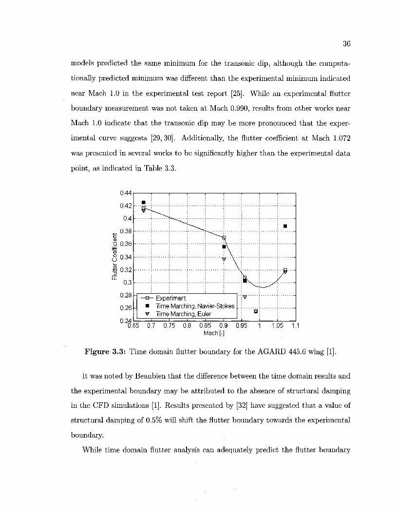
36
models predicted the same minimum for the transonic dip, although the computa
tionally predicted minimum was different than the experimental minimum indicated
near Mach 1.0 in the experimental test report [25]. While an experimental flutter
boundary measurement was not taken at Mach 0.990, results from other works near
Mach 1.0 indicate that the transonic dip may be more pronounced that the exper
imental curve suggests [29,30]. Additionally, the flutter coefficient at Mach 1.072
was presented in several works to be significantly higher than the experimental data
point, as indicated in Table 3.3.
0.44
0.42
0.4
^ 0.38 a <D
0 0.36 8= a>
Q 0.34
1 0.32
0.3 0.28
0.26
0.24
1 1
• : i 1 1 1 1 1
• \
; j f ' T ;
—a- Experiment • Time Marching, Navier-Stokes • Time Marching, Euler
i i i i i
; v
u i
— i
i •
• ' 0.65 0.7 0.75 0.8 0.85 0.9 0.95
Mach [-] 1 1.05 1.1
Figure 3.3: Time domain flutter boundary for the AGARD 445.6 wing [1]
It was noted by Beaubien that the difference between the time domain results and
the experimental boundary may be attributed to the absence of structural damping
in the CFD simulations [1]. Results presented by [32] have suggested that a value of
structural damping of 0.5% will shift the flutter boundary towards the experimental
boundary.
While time domain flutter analysis can adequately predict the flutter boundary
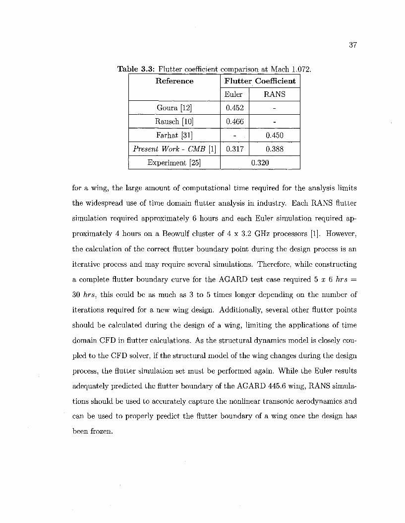
37
Table 3.3: Flutter coefficient comparison at Mach 1.072.
Reference
Goura [12]
Rausch [10]
Farhat [31]
Present Work - CMB [1]
Experiment [25]
Flutter Coefficient
Euler
0.452
0.466
-
0.317
RANS
-
-
0.450
0.388
0.320
for a wing, the large amount of computational time required for the analysis limits
the widespread use of time domain flutter analysis in industry. Each RANS flutter
simulation required approximately 6 hours and each Euler simulation required ap
proximately 4 hours on a Beowulf cluster of 4 x 3.2 GHz processors [1]. However,
the calculation of the correct flutter boundary point during the design process is an
iterative process and may require several simulations. Therefore, while constructing
a complete flutter boundary curve for the AGARD test case required 5x6 hrs =
30 hrs, this could be as much as 3 to 5 times longer depending on the number of
iterations required for a new wing design. Additionally, several other flutter points
should be calculated during the design of a wing, limiting the applications of time
domain CFD in flutter calculations. As the structural dynamics model is closely cou
pled to the CFD solver, if the structural model of the wing changes during the design
process, the flutter simulation set must be performed again. While the Euler results
adequately predicted the flutter boundary of the AGARD 445.6 wing, RANS simula
tions should be used to accurately capture the nonlinear transonic aerodynamics and
can be used to properly predict the flutter boundary of a wing once the design has
been frozen.
38
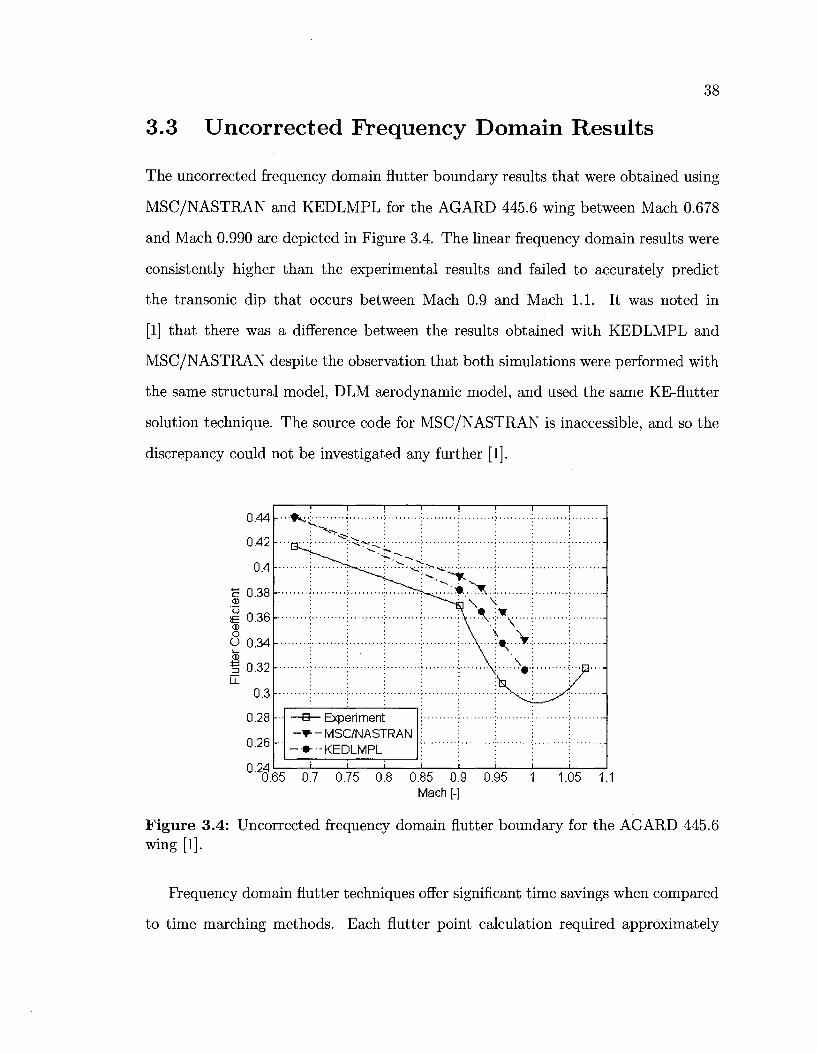
3.3 Uncorrected Frequency Domain Results
The uncorrected frequency domain flutter boundary results that were obtained using
MSC/NASTRAN and KEDLMPL for the AGARD 445.6 wing between Mach 0.678
and Mach 0.990 are depicted in Figure 3.4. The linear frequency domain results were
consistently higher than the experimental results and failed to accurately predict
the transonic dip that occurs between Mach 0.9 and Mach 1.1. It was noted in
[1] that there was a difference between the results obtained with KEDLMPL and
MSC/NASTRAN despite the observation that both simulations were performed with
the same structural model, DLM aerodynamic model, and used the same KE-flutter
solution technique. The source code for MSC/NASTRAN is inaccessible, and so the
discrepancy could not be investigated any further [1].
0.44
0.42
0.4
E 0.38 M 0.36 en
O 0.34 i
| 0.32 LL
0.3
0.28
0.26
°'264.65 0.7 0.75 0.8 0.85 0.9 0.95 1 1.05 1.1 Mach [-]
Figure 3.4: Uncorrected frequency domain flutter boundary for the AGARD 445.6 wing [1].
Frequency domain flutter techniques offer significant time savings when compared
to time marching methods. Each flutter point calculation required approximately
39
5 minutes to compute on a single 2.8 GHz processor with either MSC/NASTRAN
or with KEDLMPL. Note that the frequency domain method determines a point on
the flutter boundary as a direct result of the simulations. This is in contrast to
the time domain method where repeated iterations are required to find the flutter
boundary. The current uncorrected frequency domain technique is very attractive
for the industry due to the small amount of time involved in the calculation of the
flutter boundary despite the large inaccuracies found in the transonic regime. A
second advantage of frequency domain methods is that if the internal structure of
the wing is changed, only the structural model needs to be modified whereas the
aerodynamic model is unchanged, making this method particularly useful during the
design process.
3.4 Corrected Frequency Domain Results
The AlC-correction procedure was implemented in KEDLMPL and used nonlinear
lifting pressures from rigid-body harmonic oscillation simulations performed using the
RANS equations in CMB. Based on the work of [19], the pitching oscillations were run
for two cycles, with a resolution of 20 steps per cycle, and pressures were obtained from
the second cycle to eliminate the effect of initial transients. The reduced frequency
selected for the oscillatory simulation at a particular Mach number can correspond to
the flutter frequency predicted by the linear frequency domain solver. Alternatively,
the experimental flutter frequency at a particular Mach number can also be used for
the reduced frequency of the oscillatory CFD simulations [19].
The real and imaginary lifting pressures obtained with the DFT described in
Equations 2.28 and 2.29 were verified using CFD results produced by Silva [19] as ex
perimental pressures do not exist for the AGARD 445.6 wing. The real and imaginary
lifting pressures at 30.8% span are compared at four Mach numbers in Figure 3.5.
40
Simulations were not performed by Silva at Mach 0.990, but the unsteady pressures
obtained with CMB are shown in Figure 3.5(d). Real and imaginary pressures were
only presented by Silva at 30.8% span and were the only unsteady pressure results
available for comparison for the AGARD wing. The differences observed between
the real and imaginary pressures in Figure 3.5 may be attributed to the different
computational schemes used for the comparison. The work of Silva [19] used a finite
difference solution of the Navier-Stokes equations with an algebraic Baldwin-Lomax
turbulence model, whereas CMB used in this work used a finite volume solution of the
Navier-Stokes equations with a shear stress transport turbulence model [1]. The CFD
grid used by Silva contained 145,000 nodes with 120 points located in the chordwise
direction on the lifting surface, whereas the present work used a grid of 45,000 nodes
with 20 points located in the chordwise direction along the lifting surface. As such,
the prediction of the movement of the shock during the unsteady pitching simulations
performed in CMB may have differed from the predictions of Silva [19].
As a secondary verification of the unsteady nonlinear pressures, the amplitude
and phase from the transformed lifting pressures were compared to results from [19]
at 30.8% span at Mach 0.960 as seen in Figure 3.6.
The flutter velocity was obtained from the velocity-damping diagrams output
from the corrected frequency domain simulations. The corrected frequency domain
velocity-frequency and velocity-damping diagrams at the four simulated Mach num
bers can be seen in Figures 3.7 and 3.8. The flutter coefficient at each Mach number
was then determined using Equation 3.1.
The flutter boundary computed with the AlC-correction technique is compared to
experimental results and the computational results of Reference [19] in Figure 3.9 and
agrees well with the experiment. A comparison with results from the RANS solution
in Table 3.4 indicates that the transonic dip minimum is well characterized by the
AlC-corrected solver.
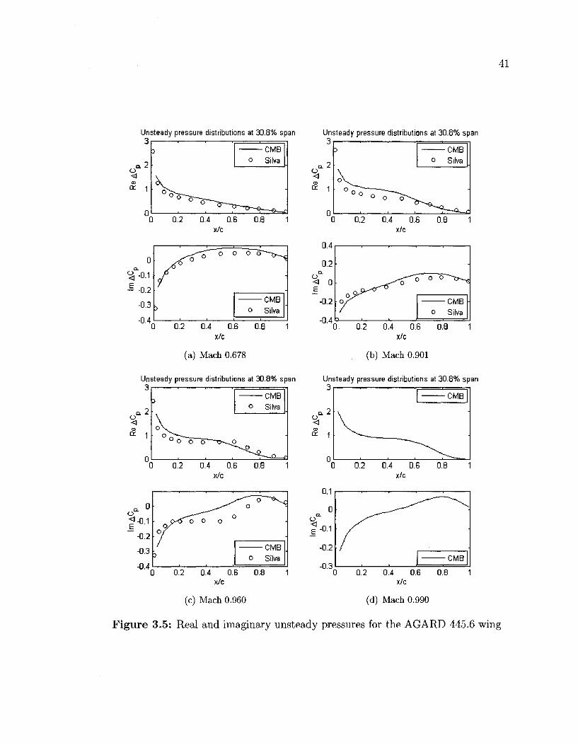
41
Unsteady pressure distributions at 30.8% span 3r
Unsteady pressure distributions at 30.8% span 3
o
0
D
• ° ^ T > ^
o Silva
0 0.2 0.4 0.6 0.8
x/c
0 •
%-0A
- -0.2
-0.3
-0.4 i>
UMU o Silva
0.2 0.4 0.6 0.8
x/c
(a) Mach 0.678 (b) Mach 0.901
Unsteady pressure distributions at 30.8% span 3
0
oV.
o Silva
>
0.2 0.4 0.6 0.8 x/c
(c) Mach 0.960
Unsteady pressure distributions at 30.8% span 3
o
QL -I
0.1
0
-0.1
-0.2
-0.3
\ ^
UMU
•
0 0.2 0.4 0.6 0.8 1 x/c
-
0 0.2 0.4 0.6 0.8 1 x/c
(d) Mach 0.990
Figure 3.5: Real and imaginary unsteady pressures for the AGARD 445.6 wing
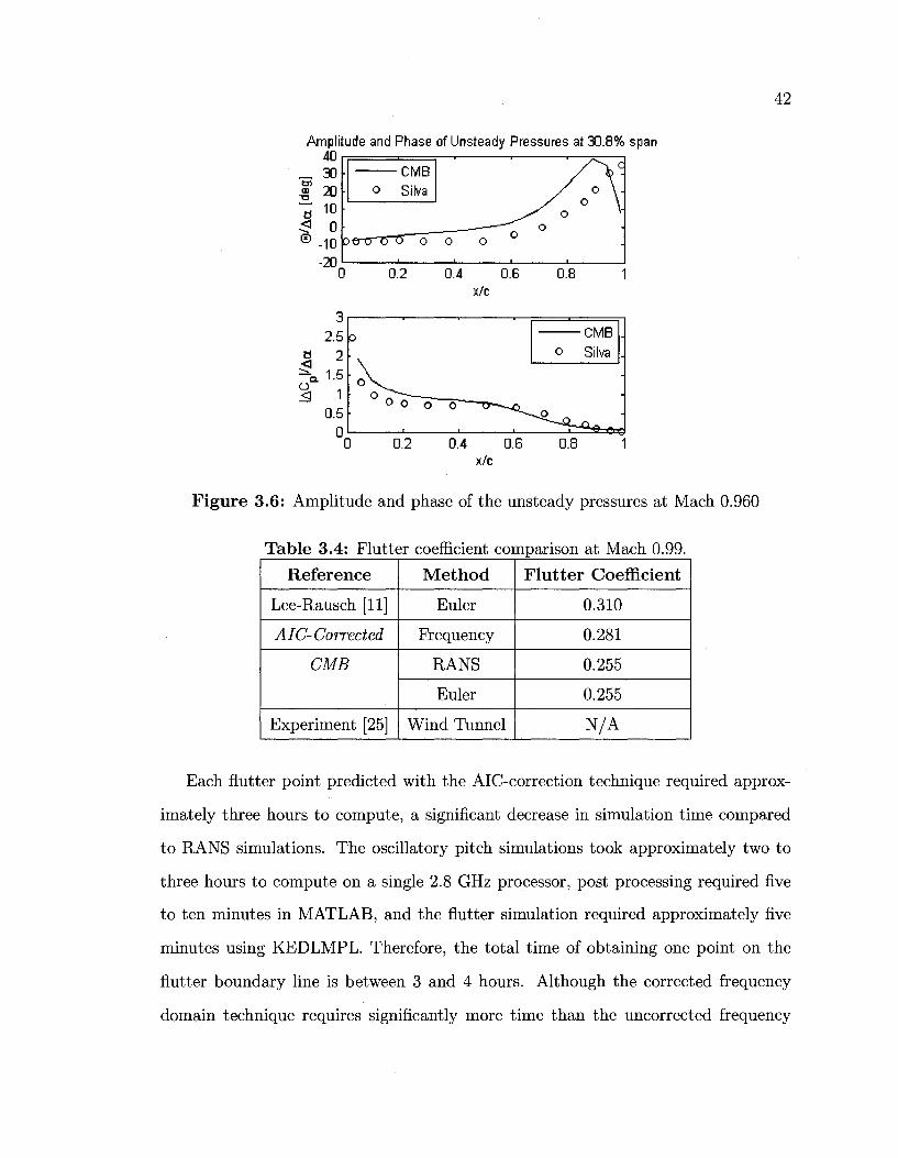
42
Amplitude and Phase of Unsteady Pressures at 30.8% span
0.4 0.6 0.8
a
a O
Figure 3.6: Amplitude and phase of the unsteady pressures at Mach 0.960
Table 3.4: Flutter coefficient comparison at Mach 0.99.
Reference
Lee-Rausch [11]
AIC-Corrected
CMB
Experiment [25]
Method
Euler
Frequency
RANS
Euler
Wind Tunnel
Flutter Coefficient
0.310
0.281
0.255
0.255
N/A
Each flutter point predicted with the AlC-correction technique required approx
imately three hours to compute, a significant decrease in simulation time compared
to RANS simulations. The oscillatory pitch simulations took approximately two to
three hours to compute on a single 2.8 GHz processor, post processing required five
to ten minutes in MATLAB, and the flutter simulation required approximately five
minutes using KEDLMPL. Therefore, the total time of obtaining one point on the
flutter boundary line is between 3 and 4 hours. Although the corrected frequency
domain technique requires significantly more time than the uncorrected frequency
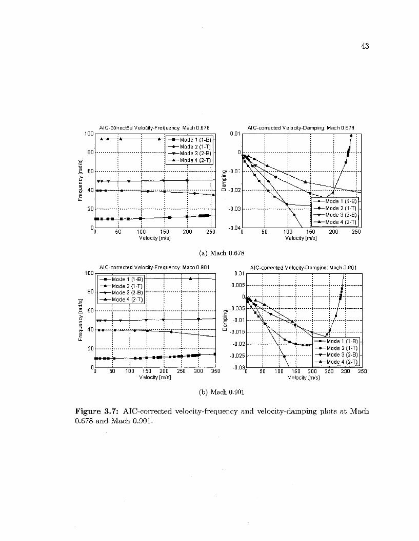
43
100
80
60
40
20
AlC-corrected Velocity-Frequency: Maori 0.678
—»-Mode2(t-T) - i ^Mode3(2-B) -- * -Mode4(2-T)
• •
i M-^-
0.01
-0.01
AlC-corrected Velocity-Damping: Mach 0.678
50 100 150 Velocity [m/s]
200 250
Q -0.02
-0.03
-0.04
'"-—^ 'y^, ~^~ — Mode 1 (1-B) -—•— Mod" i M.T I -^ * ^ M o —*—Mo
ie 3 (2-B) ie 4 (2-T)
(a) Mach 0.678
100
80
, 60
• 40
20
AlC-corrected Velocity-Frequency: Mach 0.901
I ' • Mode 1 (\-a)
-»-Mode2(1-T) • —r-Mode 3 (2-B)
- * -Mode4(2-T)
• —•- " ' t __l t
i m\ , . 1 . ^ 1
0 50 100 150 200 250 300 350 Velocity [m/s]
0.01
0.005
0
-0.005
-0.01
-0.015
-0.02
-0.025
-0.03
50 100 150 Velocity [m/s]
200 250
AlC-corrected Velocity-Damping: Mach 0.901
)\-.V^>iv^[
j . _- _^, ^ 7 ™ " ~ * " * " • "
\-f-—\ -
— Mode 1 (1-B) -- • - M o d e 2 (1-T) " - r - M o d e 3 (2-B) -—*-Mode4(2-T)
0 50 100 150 200 250 300 350 Velocity [m/s]
(b) Mach 0.901
Figure 3.7: AlC-corrected velocity-frequency and velocity-damping plots at Mach 0.678 and Mach 0.901.
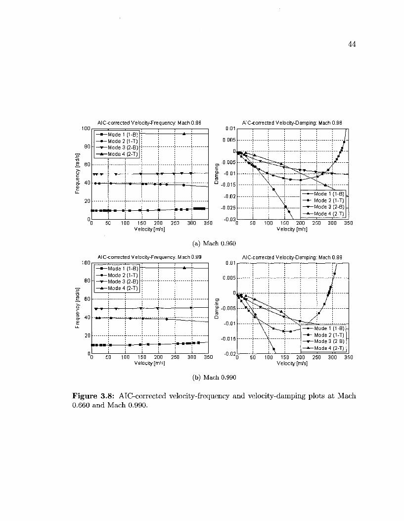
44
100
80
60
40
20
AlC-corrected Velocity-Frequency: Mach 0.96
• Mode 1 U-BJ —»-Made2(1-T)
• -^ -Mode3(2-B) - * -Mode4(2 -T)
- ; - - - ] - • - - :
; ' T ; T T
| ! | |
Q
0 50 100 150 200 250 300 350 Velocity [m/s]
0.01
0.005
0
-0.005
-0.01
•0.015
-0.02
•0.025
-0.03
AlC-corrected Velocity-Damping: Mach 0.96
..7^%Jrr^^!- \ j .yf.....
I ^ ^ ——Mode 1 (1-B) „ - * -Mode2(1-T) ~ - t -Mode3(2 -B) --J»-Mode4(2-T)
0 50 100 150 200 250 300 350 Velocity [m/s]
(a) M a c h 0.960
100
80
60
40
20
AlC-corrected Velocity-Frequency: Mach 0.99
—•—Mode 1 I I -BJ — Mode2(1-T)
• —*-Mode3(2-B) - * -Mode4(2-T)
w-r 1 ^
: _ L i m ...
D
0 50 100 150 200 250 300 350 Velocity [m/s]
0.01
0.005
0
-0.005
-0.01
-0.015
-0.02
AlC-corrected Velocity-Damping: Mach 0.99
i i i ! I I
.„S\
-—Mode 1 (1-B) -- * -Mode2(1-T) - * - l u lode 3 (2-B)
lode 4 (2-T)
0 50 100 150 200 250 300 350 Velocity [m/s]
(b) M a c h 0 .990
Figure 3.8: AlC-corrected velocity-frequency and velocity-damping plots at Mach 0 .660 a n d M a c h 0 . 9 9 0 .
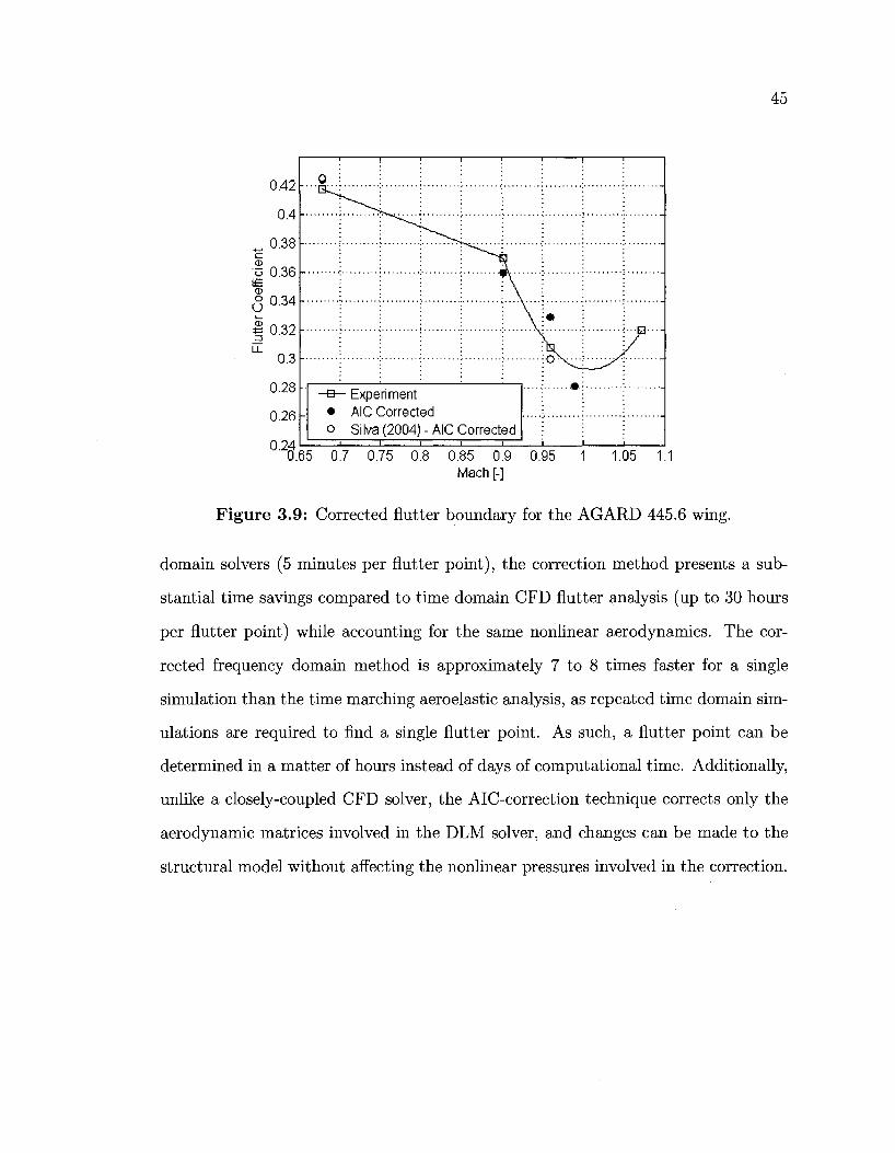
45
it: (D O O i <D 4=1 3
0.42
0.4
0.38
0.36
0.34
0.32
0.3
0.28
0.26
0.24
0 I i
- B — Experiment • AIC Cormrt-firi o Silva (2004) - AIC Corrected
i i i i ,
*
o\^-—y{ -
' i
'0.65 0.7 0.75 0.8 0.85 0.9 0.95 Mach [-]
1 1.05 1.1
Figure 3.9: Corrected flutter boundary for the AGARD 445.6 wing.
domain solvers (5 minutes per flutter point), the correction method presents a sub
stantial time savings compared to time domain CFD flutter analysis (up to 30 hours
per flutter point) while accounting for the same nonlinear aerodynamics. The cor
rected frequency domain method is approximately 7 to 8 times faster for a single
simulation than the time marching aeroelastic analysis, as repeated time domain sim
ulations are required to find a single flutter point. As such, a flutter point can be
determined in a matter of hours instead of days of computational time. Additionally,
unlike a closely-coupled CFD solver, the AlC-correction technique corrects only the
aerodynamic matrices involved in the DLM solver, and changes can be made to the
structural model without affecting the nonlinear pressures involved in the correction.
3.5 Conclusion
46
Computational transonic flutter analysis was performed on the AGARD 445.6 wing in
the time domain and in the frequency domain. A procedure was developed to correct
the frequency domain flutter boundary by accounting for the nonlinear aerodynamics
present within the transonic regime using rigid body unsteady pitching-motion CFD
simulations. Time domain aeroelastic CFD simulations and AlC-corrected frequency
domain results both adequately predicted the flutter boundary of the AGARD 445.6
wing. The corrected frequency domain approach however, required significantly less
computational time and fewer computational resources than the time domain CFD
analysis, rendering the method attractive for industrial use during the design phase
of a wing. The corrected frequency domain approach is ideal for iterative design pro
cesses since the oscillatory pitch aerodynamic simulation only needs to be performed
once per Mach number and is not affected by the structural model. As such, the effect
of structural changes on the flutter boundary can be assessed very rapidly during the
design process.
3.6 Recommendations and Future Work
As the RANS time domain and AlC-corrected frequency domain solutions both have
useful industrial applications, further validation should be conducted on another tran
sonic wing model that more closely resembles a commercial transport wing. Potential
candidates could include the YXX wing, the PAPA wing, or the LANN wing. The
LANN wing experiment was performed in the 1980s and uses a supercritical airfoil
but was never tested to flutter because of the operational limits of the wind tunnel.
Aerodynamic and structural information is available however, and RANS simulations
could be used as the benchmark comparison to the AlC-corrected results.
47
The capability of CMB and the AlC-correction method to perform time and fre
quency domain flutter analysis of a wing with a pod-mounted engine should be inves
tigated. The simulation of a wing with an engine would further increase the industrial
applications of the AlC-corrected flutter technique.
Part II
Rotary-wing Aeroelasticity
48
Chapter 4
Introduction to Wind Turbine Technology
In the second part of this thesis, the aeroelastic simulations of a wind turbine mod
eled with a vortex particle wake and a nonlinear structural model will be presented.
The focus was on identifying and developing a computational tool feasible for prac
tical industrial applications that is both computationally robust and efficient. The
chapter will start with a historical review of wind turbine development, followed by
a review of the computational tools currently used for predicting their performance.
This will help to identify the need for more accurate aerodynamic and aeroelastic
simulations. Aeroelastic simulations of a benchmark experimental wind turbine test
are then presented.
4.1 Historical Developments
Wind energy is rapidly becoming a viable source of renewable energy and worldwide
installed wind energy capacity is growing by 25% annually [33]. The modern three-
bladed horizontal axis wind turbine is now used exclusively for electrical generation,
and represents the culmination of thousands of years of design and development of
ancient windmills.
Early windmills were typically used for milling grain or pumping water and may
49
50
have been invented between 2,000 and 3,000 years ago in Egypt, though the exis
tence of these early windmills is disputed in literature [34,35]. The first formally
documented windmills appeared in Persia and Afghanistan between the 7th and 12th
centuries. These early windmills were vertical axis windmills used for milling grains,
as seen in Figure 4.1(a) [34]. The European horizontal axis windmill was developed
independently in northern Europe between the 12th and 18th centuries. These were
traditionally drag-driven windmills with four wooden or cloth covered sails that were
used for pumping water, for milling grain, or as sawmills, as depicted in Figure 4.1(b).
Continuous improvements and refinements were made to the towers, sails and control
devices of European windmills between the 12th and 17th centuries, but these were
conducted on a trial and error basis [35]. It wasn't until the 17th and 18th centuries
that windmill design and aerodynamics were influenced by and studied by Leibniz,
Bernoulli, and Euler [34]. A third distinct type of windmill was developed in the
United States by Daniel Halladay in the late 19th century, an example of which can
be seen in Figure 4.1(c). The American wind turbine, which was primarily used for
irrigation and pumping, was the first successful commercial windmill and had sold
over six million examples by 1930 [34].
The development of wind turbines for electrical generation began in the late 19th
century with the construction of the Brush windmill in Ohio. The Brush turbine
had 144 thin blades, a rotor diameter of 17 m, and supplied 12 kW of DC power for
charging batteries [35]. This turbine successfully generated power for twenty years
before being decommissioned and was the last example of a large multi-vane wind
turbine. Shortly after the Brush windmill was completed, the La Cour windmill was
built in Denmark in 1891 and improved upon many of the technical achievements
of the European windmills. The La Cour windmill had four twisted and cambered
blades that had been tested and developed in a wind tunnel. Successive industrialized
iterations of this design produced between 10 and 35 kW of electricity [34].
51
The precursor to the modern wind turbine however, was the Smith-Putnam tur
bine developed in 1941 in Vermont, whose rotor blades were designed in part by von
Karman. The Smith-Putnam turbine was the first megawatt scale turbine, as seen in
Figure 4.1(d), and produced up to 1.25 MW of power. The turbine had a two-bladed
stainless steel rotor with a diameter of 53 m and featured many novel innovations
including full-span pitch control, flapping hinges to alleviate load imbalances, and ac
tive yaw control. The Smith-Putnam turbine fed electricity into the local grid for four
years before developing large cracks in its rotor. The turbine had to be dismantled
as there were no funds to repair its rotor, but it pioneered most of the technologies
that have been implemented in modern turbines [34].
Interest in wind turbines diminished following the Second World War because of
cheap oil imports and interest in nuclear energy [36]. However, the United States
launched an ambitious research and development program for new turbine designs
after the energy crisis in the 1970s. New experimental wind turbines were tested and
a large number of wind farms were built in the United States throughout the mid
1980s [35]. The vast majority of new wind farm developments since the 1980s have
been built in Europe as interest again faded in North America due to inexpensive
oil in the 1990s and Europe now accounts for 60% of the worldwide wind generating
capacity [33].
There has been a push to increase the rotor size of commercial turbines through
out the past twenty years due to the economy of scale, increased power generation
requirements, and more effective land use. The increase in turbine size and power
since 1980 is represented schematically in Figure 4.2. Though current designs exist
for 5 MW turbines, the typical size of new turbines in wind farms is between 2 and
3 MW with rotor diameters of 80 m to 100 m.
Wind turbine research in Canada reached its peak in the 1970s and 1980s and
focused on the development of Darrieus vertical-axis wind turbines [37]. The research
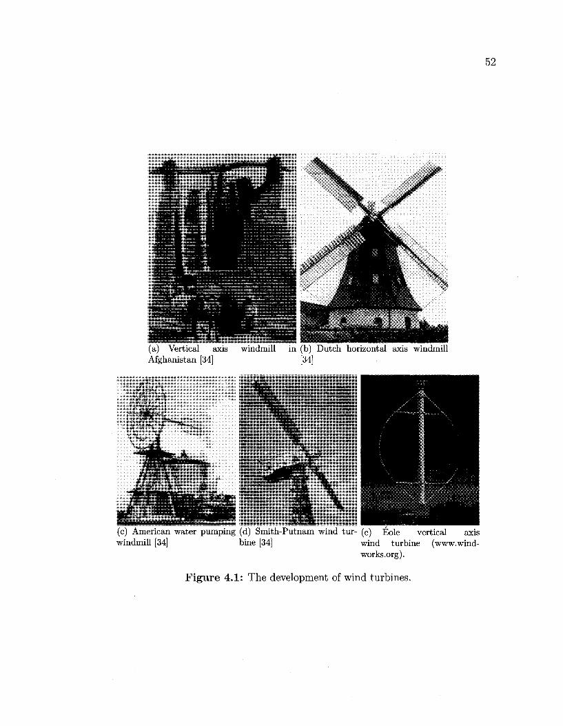
52
(a) Vertical axis windmill in (b) Dutch horizontal axis windmill Afghanistan [34] [34]
(c) American water pumping (d) Smith-Putnam wind tur- (e) Eole vertical axis windmill [34] bine [34] wind turbine (www.wind-
works.org).
Figure 4.1: The development of wind turbines.
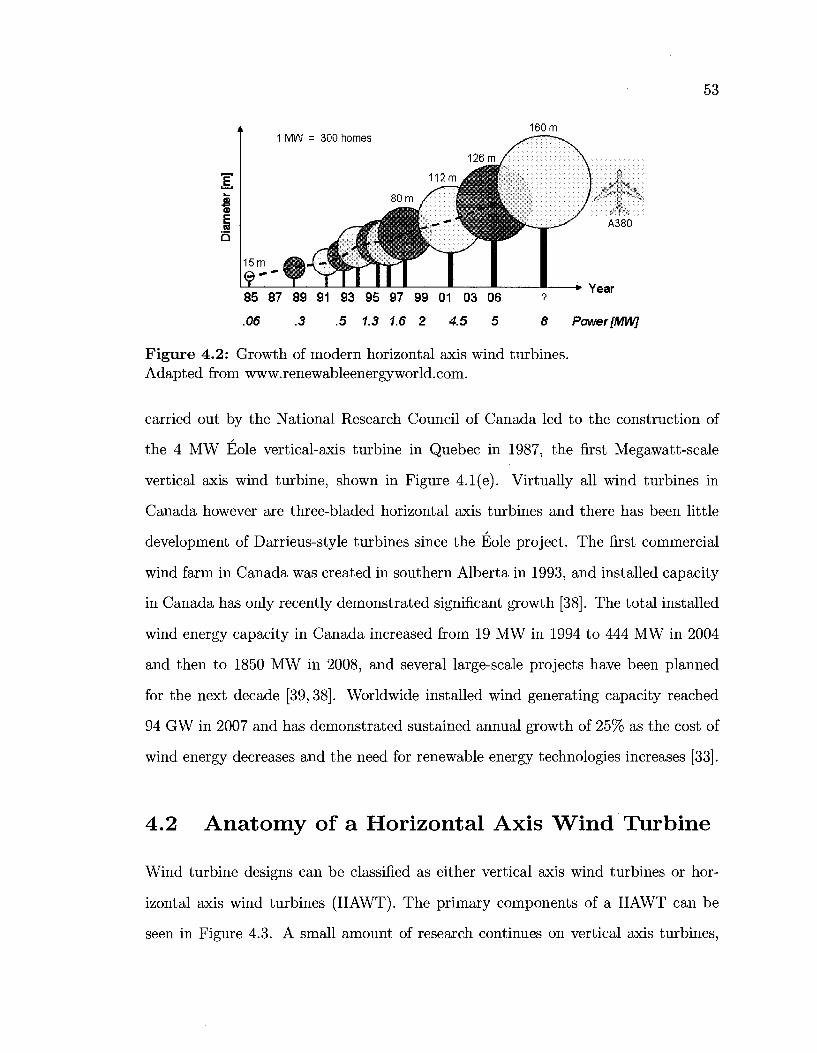
53
85 87 89 91 93 95 97 99 01 03 06 ?
.06 .3 .5 1.3 1.6 2 4.5 5 8 PowerfMW]
Figure 4.2: Growth of modern horizontal axis wind turbines. Adapted from www.renewableenergyworld.com.
carried out by the National Research Council of Canada led to the construction of
the 4 MW Eole vertical-axis turbine in Quebec in 1987, the first Megawatt-scale
vertical axis wind turbine, shown in Figure 4.1(e). Virtually all wind turbines in
Canada however are three-bladed horizontal axis turbines and there has been little
development of Darrieus-style turbines since the Eole project. The first commercial
wind farm in Canada was created in southern Alberta in 1993, and installed capacity
in Canada has only recently demonstrated significant growth [38]. The total installed
wind energy capacity in Canada increased from 19 MW in 1994 to 444 MW in 2004
and then to 1850 MW in 2008, and several large-scale projects have been planned
for the next decade [39,38]. Worldwide installed wind generating capacity reached
94 GW in 2007 and has demonstrated sustained annual growth of 25% as the cost of
wind energy decreases and the need for renewable energy technologies increases [33].
4.2 Anatomy of a Horizontal Axis Wind Turbine
Wind turbine designs can be classified as either vertical axis wind turbines or hor
izontal axis wind turbines (HAWT). The primary components of a HAWT can be
seen in Figure 4.3. A small amount of research continues on vertical axis turbines,
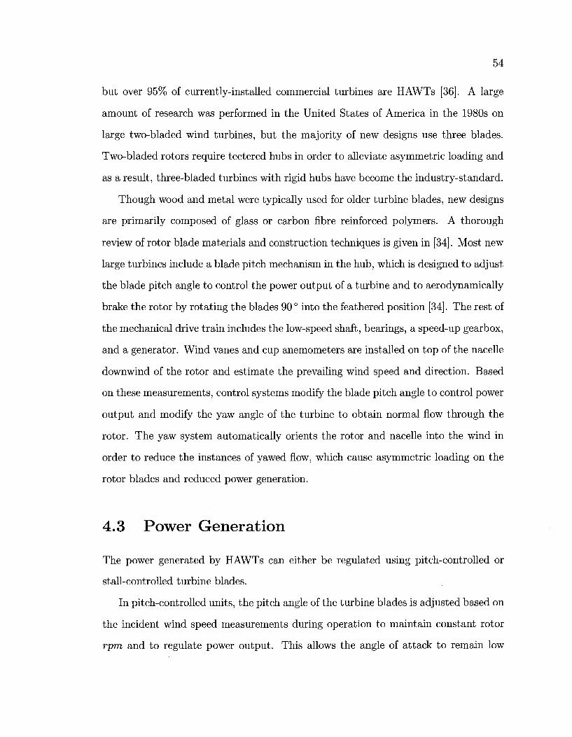
54
but over 95% of currently-installed commercial turbines are HAWTs [36]. A large
amount of research was performed in the United States of America in the 1980s on
large two-bladed wind turbines, but the majority of new designs use three blades.
Two-bladed rotors require teetered hubs in order to alleviate asymmetric loading and
as a result, three-bladed turbines with rigid hubs have become the industry-standard.
Though wood and metal were typically used for older turbine blades, new designs
are primarily composed of glass or carbon fibre reinforced polymers. A thorough
review of rotor blade materials and construction techniques is given in [34]. Most new
large turbines include a blade pitch mechanism in the hub, which is designed to adjust
the blade pitch angle to control the power output of a turbine and to aerodynamicaUy
brake the rotor by rotating the blades 90 ° into the feathered position [34]. The rest of
the mechanical drive train includes the low-speed shaft, bearings, a speed-up gearbox,
and a generator. Wind vanes and cup anemometers are installed on top of the nacelle
downwind of the rotor and estimate the prevailing wind speed and direction. Based
on these measurements, control systems modify the blade pitch angle to control power
output and modify the yaw angle of the turbine to obtain normal flow through the
rotor. The yaw system automatically orients the rotor and nacelle into the wind in
order to reduce the instances of yawed flow, which cause asymmetric loading on the
rotor blades and reduced power generation.
4.3 Power Generation
The power generated by HAWTs can either be regulated using pitch-controlled or
stall-controlled turbine blades.
In pitch-controlled units, the pitch angle of the turbine blades is adjusted based on
the incident wind speed measurements during operation to maintain constant rotor
rpm and to regulate power output. This allows the angle of attack to remain low
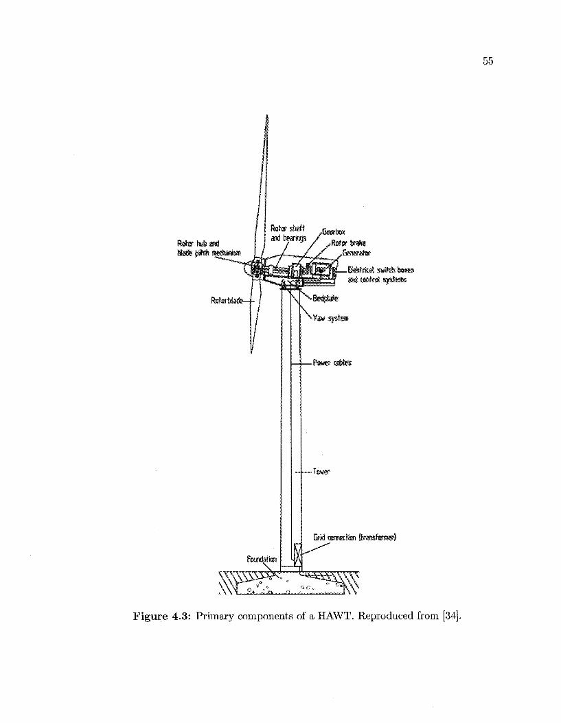
55
ftoftr hub awl M a * pitch
faftbtim
EfekfrM switch feme and c « W Sfsfas
IY*'
-Power aWes
-Twer
Grid
* ^
Figure 4.3: Primary components of a HAWT. Reproduced from [34].
56
throughout the operational regime of the turbine and allows the rated turbine power
to be strictly controlled over the rated wind speeds. If the incident velocity is too
high and risks damaging a machine, the blades are rotated to the feathered position
and the turbine is stopped [34].
Stall-controlled turbines however, have a fixed blade pitch angle and are designed
to operate in the fully stalled flow regime over the range of rated wind speeds. Stall-
regulated blades rely on passive stall control to regulate the power generated by the
rotor and to maintain constant rotor rpm. This phenomena is described in Figure
4.4 where a turbine blade section is shown at both a low wind speed and a high
wind speed. The fixed blade pitch angle (0) is assumed to be positive towards the
feathered position, and the tangential velocity (Vrot) of a particular spanwise section
is assumed to be constant throughout the operational range of the turbine. Figure
4.4 demonstrates that the blade section angle of attack (a) will increase with the
wind speed. In wind speeds that correspond to the rated power of a turbine, a will
be higher than the critical angle of attack (acmr), where the blade section begins
to experience stalled flow. At the rated turbine power, a varying degree of stall
occurs over the blade sections and the rotor power is controlled by the amount of
aerodynamic stall occurring over the span of the rotor blade. Stall-regulated rotors
are typically only used on smaller wind turbines and suffer from restrictions for grid
connection.
Wind turbine performance is described by a power curve, which identifies the cut-
in velocity, the rated power, the rated wind velocity, and the cut-out velocity. The
cut-in velocity refers to the velocity where the turbine can start to deliver power and
typically occurs around 3 to 4 m/s. The rated wind velocity is the wind speed at
which the rated generator power is reached, and the cut-out velocity is the highest
wind velocity at which the turbine can be operated without damage [34]. If the
wind velocity exceeds the cut-out velocity, the turbine is braked aerodynamically or
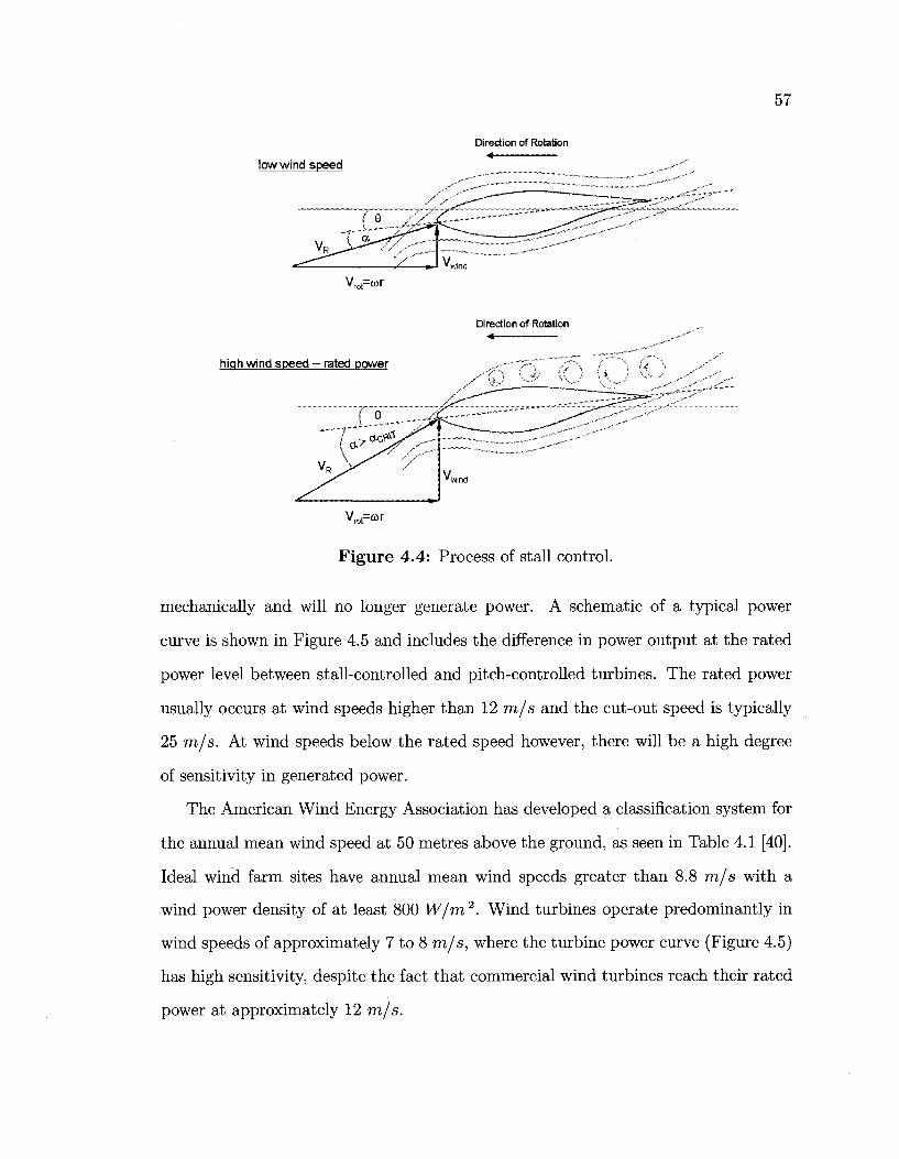
57
Direction of Rotation • *
low wind speed
Direction of Rotation •4
high wind speed - rated power „:r-
Figure 4.4: Process of stall control.
mechanically and will no longer generate power. A schematic of a typical power
curve is shown in Figure 4.5 and includes the difference in power output at the rated
power level between stall-controlled and pitch-controlled turbines. The rated power
usually occurs at wind speeds higher than 12 m/s and the cut-out speed is typically
25 m/s. At wind speeds below the rated speed however, there will be a high degree
of sensitivity in generated power.
The American Wind Energy Association has developed a classification system for
the annual mean wind speed at 50 metres above the ground, as seen in Table 4.1 [40].
Ideal wind farm sites have annual mean wind speeds greater than 8.8 m/s with a
wind power density of at least 800 W/m2. Wind turbines operate predominantly in
wind speeds of approximately 7 to 8 m/s, where the turbine power curve (Figure 4.5)
has high sensitivity, despite the fact that commercial wind turbines reach their rated
power at approximately 12 m/s.
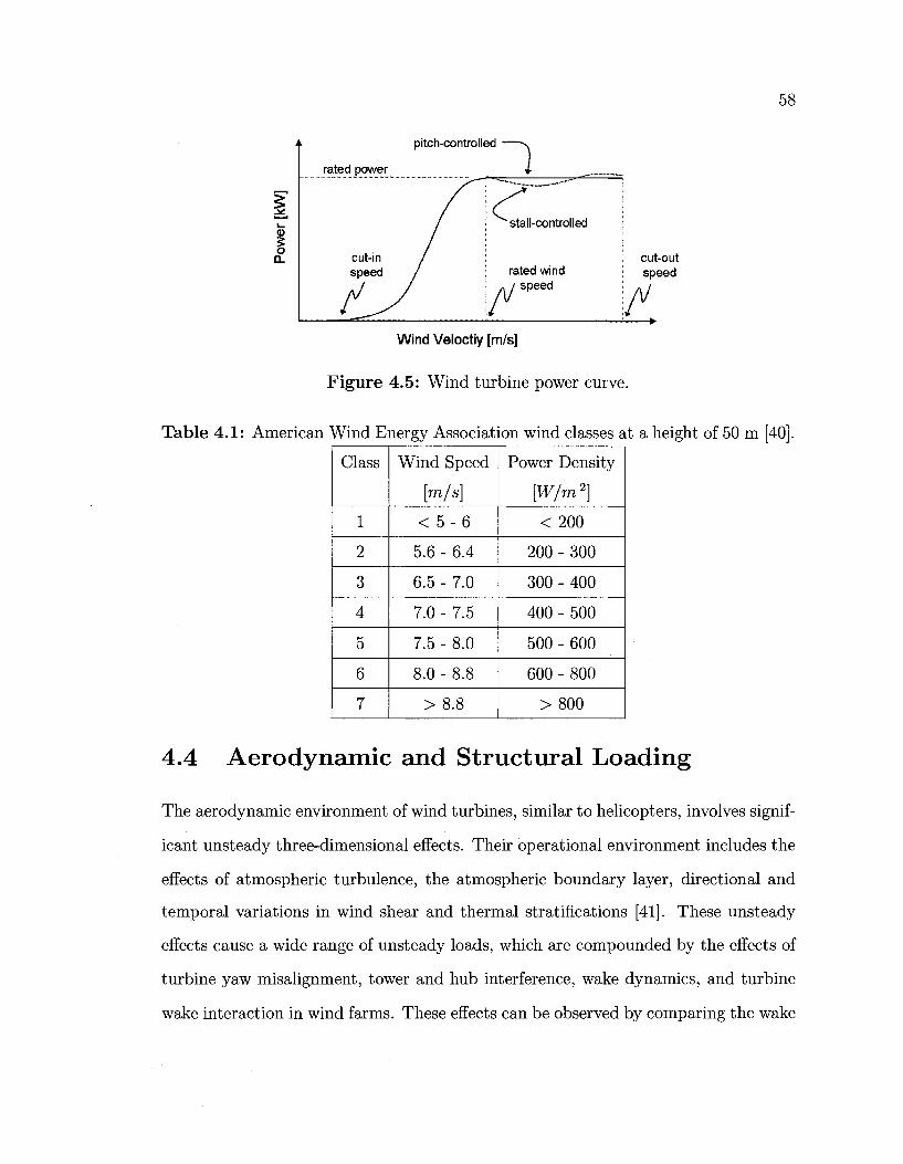
58
§ Q. cut-out
speed
Wind Veloctiy [m/s]
Figure 4.5: Wind turbine power curve.
Table 4.1: American Wind Energy Association wind classes at a height of 50 m [40].
Class
1
2
3
4
5
6
7
Wind Speed
[m/s]
< 5 - 6
5.6 - 6.4
6.5 - 7.0
7.0 - 7.5
7.5 - 8.0
8.0 - 8.8
> 8.8
Power Density
[W/m2]
< 200
200 - 300
300 - 400
400 - 500
500 - 600
600 - 800
> 800
4.4 Aerodynamic and Structural Loading
The aerodynamic environment of wind turbines, similar to helicopters, involves signif
icant unsteady three-dimensional effects. Their operational environment includes the
effects of atmospheric turbulence, the atmospheric boundary layer, directional and
temporal variations in wind shear and thermal stratifications [41]. These unsteady
effects cause a wide range of unsteady loads, which are compounded by the effects of
turbine yaw misalignment, tower and hub interference, wake dynamics, and turbine
wake interaction in wind farms. These effects can be observed by comparing the wake
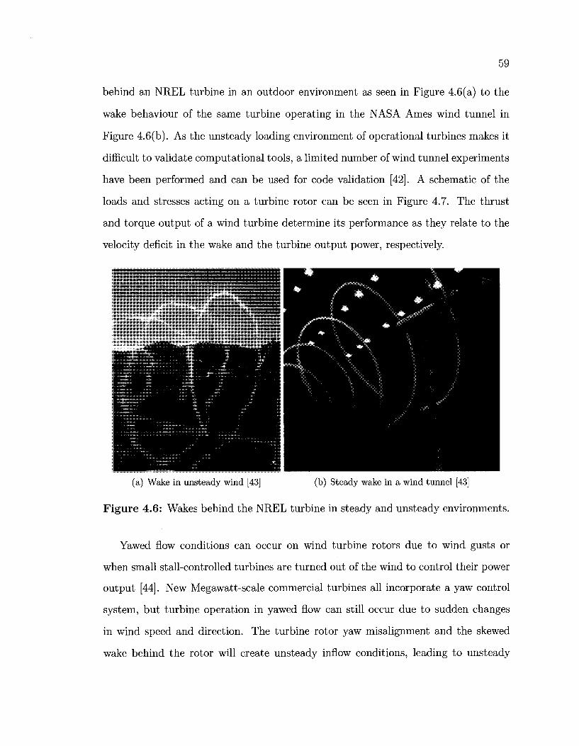
59
behind an NREL turbine in an outdoor environment as seen in Figure 4.6(a) to the
wake behaviour of the same turbine operating in the NASA Ames wind tunnel in
Figure 4.6(b). As the unsteady loading environment of operational turbines makes it
difficult to validate computational tools, a limited number of wind tunnel experiments
have been performed and can be used for code validation [42]. A schematic of the
loads and stresses acting on a turbine rotor can be seen in Figure 4.7. The thrust
and torque output of a wind turbine determine its performance as they relate to the
velocity deficit in the wake and the turbine output power, respectively.
(a) Wake in unsteady wind [43] (b) Steady wake in a wind tunnel [43]
Figure 4.6: Wakes behind the NREL turbine in steady and unsteady environments.
Yawed flow conditions can occur on wind turbine rotors due to wind gusts or
when small stall-controlled turbines are turned out of the wind to control their power
output [44]. New Megawatt-scale commercial turbines all incorporate a yaw control
system, but turbine operation in yawed flow can still occur due to sudden changes
in wind speed and direction. The turbine rotor yaw misalignment and the skewed
wake behind the rotor will create unsteady inflow conditions, leading to unsteady
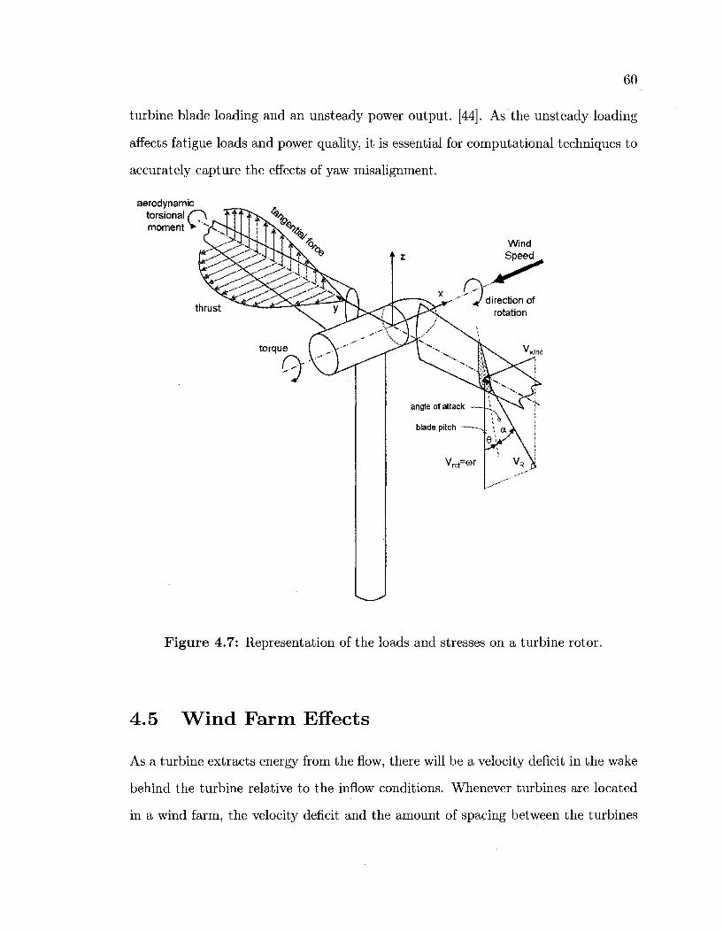
60
turbine blade loading and an unsteady power output. [44]. As the unsteady loading
affects fatigue loads and power quality, it is essential for computational techniques to
accurately capture the effects of yaw misalignment.
aerodynamic torsional (~\
> -moment Wind Speed
thrust
Figure 4.7: Representation of the loads and stresses on a turbine rotor.
4.5 Wind Farm Effects
As a turbine extracts energy from the flow, there will be a velocity deficit in the wake
behind the turbine relative to the inflow conditions. Whenever turbines are located
in a wind farm, the velocity deficit and the amount of spacing between the turbines
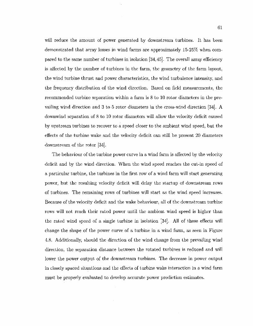
61
will reduce the amount of power generated by downstream turbines. It has been
demonstrated that array losses in wind farms are approximately 15-25% when com
pared to the same number of turbines in isolation [34,45]. The overall array efficiency
is affected by the number of turbines in the farm, the geometry of the farm layout,
the wind turbine thrust and power characteristics, the wind turbulence intensity, and
the frequency distribution of the wind direction. Based on field measurements, the
recommended turbine separation within a farm is 8 to 10 rotor diameters in the pre
vailing wind direction and 3 to 5 rotor diameters in the cross-wind direction [34]. A
downwind separation of 8 to 10 rotor diameters will allow the velocity deficit caused
by upstream turbines to recover to a speed closer to the ambient wind speed, but the
effects of the turbine wake and the velocity deficit can still be present 20 diameters
downstream of the rotor [34].
The behaviour of the turbine power curve in a wind farm is affected by the velocity
deficit and by the wind direction. When the wind speed reaches the cut-in speed of
a particular turbine, the turbines in the first row of a wind farm will start generating
power, but the resulting velocity deficit will delay the startup of downstream rows
of turbines. The remaining rows of turbines will start as the wind speed increases.
Because of the velocity deficit and the wake behaviour, all of the downstream turbine
rows will not reach their rated power until the ambient wind speed is higher than
the rated wind speed of a single turbine in isolation [34]. All of these effects will
change the shape of the power curve of a turbine in a wind farm, as seen in Figure
4.8. Additionally, should the direction of the wind change from the prevailing wind
direction, the separation distance between the rotated turbines is reduced and will
lower the power output of the downstream turbines. The decrease in power output
in closely spaced situations and the effects of turbine wake interaction in a wind farm
must be properly evaluated to develop accurate power prediction estimates.
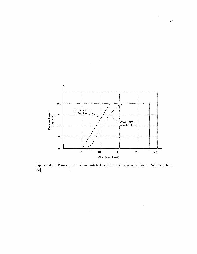
62
100
Ji 75
11 | O 50
25
k
Sir Tur
gle bine , -v.
• ^ ^ i
J JL. ., , C
j i
|
Wind Farm haracteristics
|
|
' •
10 15
Wind Speed [m/s]
20 25
Figure 4.8: Power curve of an isolated turbine and of a wind farm. Adapted from [34].
Chapter 5
A Review of Wind Turbine Aeroelasticity
The prediction of the annual energy output of a wind turbine or wind farm is directly
dependent upon the accuracy of the computational techniques used in commercial
or research codes. These techniques consist primarily of blade element methods,
actuator disk methods, potential flow methods, and full CFD methods, though a
number of empirical wake models have been developed for commercial analysis tools.
Wind farm software packages rely on simplified wake modeling to evaluate the effect
of the wakes of upstream turbines on downstream rotors. While wake models are
generally valid at the conditions under which they were developed, they rely on many
empirical assumptions [46].
A thorough review of the aerodynamic techniques that are used to resolve the near
and far wakes of wind turbines was published by Vermeer et al in 2003 [42]. This
review also summarized the major experimental efforts that have been undertaken
to characterize the loads and wakes produced by wind turbines. A follow-up review
in 2006 by Hansen summarized the aerodynamic and aeroelastic techniques that are
presently being used to study wind turbine loads [47]. Recent experiments have
demonstrated that there are many inaccuracies in the prediction of wind turbine
and wind farm performance [48]. The assumptions, merits, and inadequacies of the
primary wind turbine and wake prediction techniques will be discussed in this Section.
63
64
5.1 Wind Turbine Wake Modeling
A number of commercial software packages have been developed to plan wind farm
layouts, to calculate annual energy yields, to perform financial analysis, and to predict
the wake losses that occur in wind farms. Proper characterization of turbine wakes is
essential for accurate energy predictions in order to both determine the wind velocity
deficit at downstream turbines and to accurately capture the physics of the flow
around a single rotor. All commercial wind farm programs contain a database of wind
turbine thrust and power coefficients that can be imported from existing designs or
determined from aerodynamic solvers in advance.
5.1.1 Wake Models
The PARK wake model, developed by Katie et al [49], is two-dimensional model
that uses momentum theory to predict the initial velocity deficit behind a turbine.
A rectangular velocity profile is initiated two diameters downstream of the turbine
and the wake is assumed to expand linearly downstream according to an empirical
wake decay constant, as seen in Figure 5.1. As the centerline of the wake follows
the terrain in the model, the mapped terrain must be relatively homogeneous to
approximate the physical behaviour of the wake. The PARK model, though very
rapid, does not properly represent the physical behaviour of the wake and relies on
momentum theory, which is invalid in many turbine loading conditions.
In the late 1980s, Ainslie developed a wind turbine wake model that formed the
basis for the models that have been implemented in the wind farm software GH
Windfarmer [51,50] and FLaP [52]. The Ainslie model is a semi-empirical wake model
that is based on the discretization of the inviscid thin layer Navier-Stokes equations
and is depicted in Figure 5.2.
In the Ainslie model, it is assumed that the flow is axisymmetric, fully turbulent,
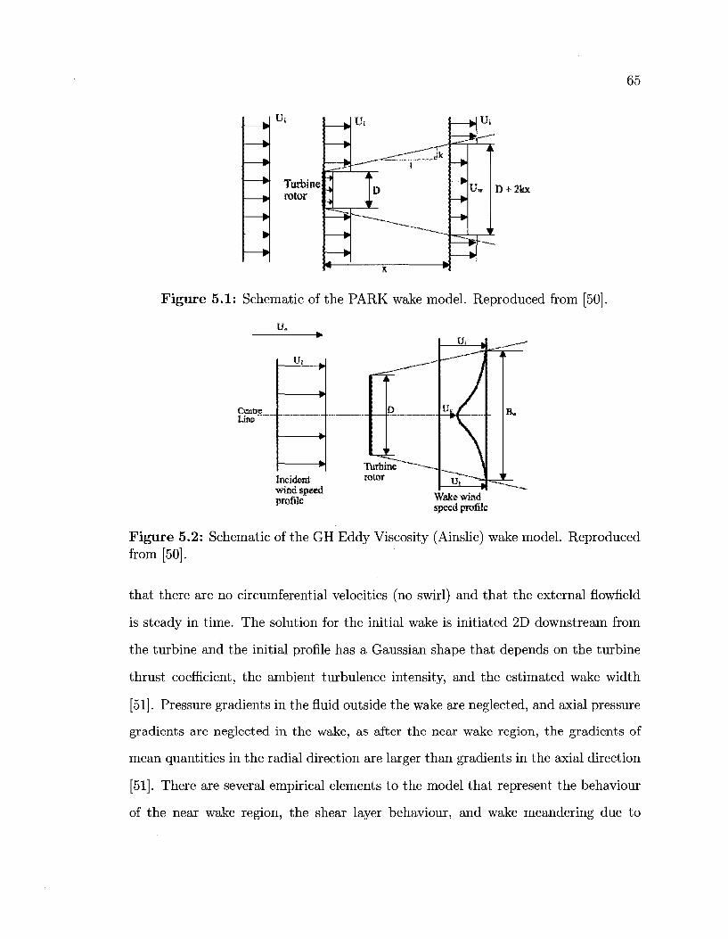
65
Figure 5.1: Schematic of the PARK wake model. Reproduced from [50].
Figure 5.2: Schematic of the GH Eddy Viscosity (Ainslie) wake model. Reproduced from [50].
that there are no circumferential velocities (no swirl) and that the external nowfield
is steady in time. The solution for the initial wake is initiated 2D downstream from
the turbine and the initial profile has a Gaussian shape that depends on the turbine
thrust coefficient, the ambient turbulence intensity, and the estimated wake width
[51]. Pressure gradients in the fluid outside the wake are neglected, and axial pressure
gradients are neglected in the wake, as after the near wake region, the gradients of
mean quantities in the radial direction are larger than gradients in the axial direction
[51]. There are several empirical elements to the model that represent the behaviour
of the near wake region, the shear layer behaviour, and wake meandering due to
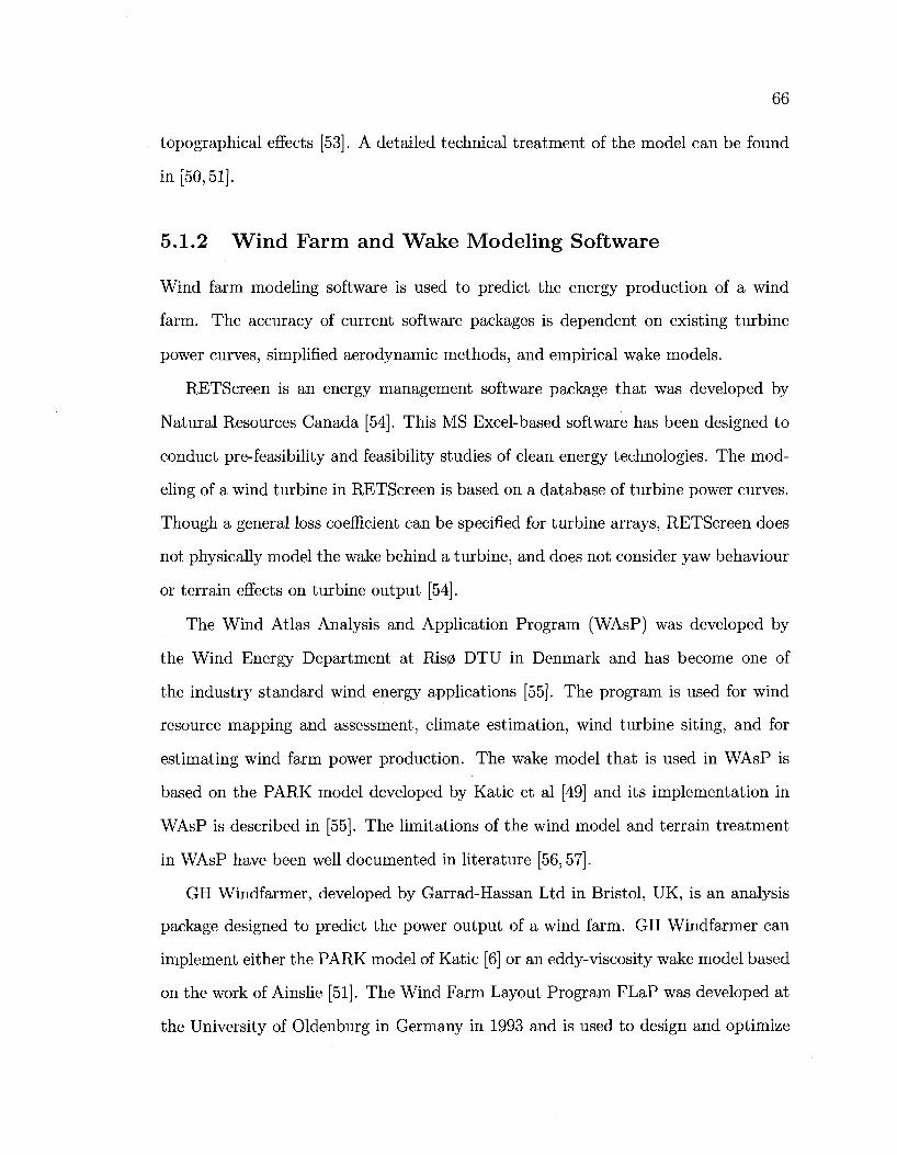
66
topographical effects [53]. A detailed technical treatment of the model can be found
in [50,51].
5.1.2 Wind Farm and Wake Modeling Software
Wind farm modeling software is used to predict the energy production of a wind
farm. The accuracy of current software packages is dependent on existing turbine
power curves, simplified aerodynamic methods, and empirical wake models.
RETScreen is an energy management software package that was developed by
Natural Resources Canada [54]. This MS Excel-based software has been designed to
conduct pre-feasibility and feasibility studies of clean energy technologies. The mod
eling of a wind turbine in RETScreen is based on a database of turbine power curves.
Though a general loss coefficient can be specified for turbine arrays, RETScreen does
not physically model the wake behind a turbine, and does not consider yaw behaviour
or terrain effects on turbine output [54].
The Wind Atlas Analysis and Application Program (WAsP) was developed by
the Wind Energy Department at Ris0 DTU in Denmark and has become one of
the industry standard wind energy applications [55]. The program is used for wind
resource mapping and assessment, climate estimation, wind turbine siting, and for
estimating wind farm power production. The wake model that is used in WAsP is
based on the PARK model developed by Katie et al [49] and its implementation in
WAsP is described in [55]. The limitations of the wind model and terrain treatment
in WAsP have been well documented in literature [56,57].
GH Windfarmer, developed by Garrad-Hassan Ltd in Bristol, UK, is an analysis
package designed to predict the power output of a wind farm. GH Windfarmer can
implement either the PARK model of Katie [6] or an eddy-viscosity wake model based
on the work of Ainslie [51]. The Wind Farm Layout Program FLaP was developed at
the University of Oldenburg in Germany in 1993 and is used to design and optimize
67
wind farm layouts and similar to GH Windfarmer, models turbine wakes using the
Ainslie model [58].
ECN Wakefarm is a wind farm analysis package developed at the Energy Research
Centre of the Netherlands that is based on the single-turbine UPMWAKE code de
veloped at the Universidad Polytecnica de Madrid [59]. Wakefarm uses blade element
momentum theory to calculate the axial induction factor and the thrust coefficient
of a turbine. In 2006, several improvements were made to Wakefarm to more accu
rately reflect the physical nature of the wake. In the new version of the code, the
axial pressure gradient is prescribed as an external force instead of being neglected
and wake expansion is enforced as well [59]. The pressure gradient is calculated a
priori using an axisymmetric vortex tube solution. This potential flow method treats
the turbine as an actuator disc and uses the axial induction factor determined with
the blade element method. Pressure gradients are calculated for a range of induction
factors and are stored in a database. During simulations, Wakefarm then determines
the pressure gradient for each turbine in the wind farm from a lookup table based on
the axial induction factor [59].
5.1.3 Wake Model Validation
The GH Eddy Viscosity wake model has been validated against a wind tunnel ex
periment performed by Ainslie and Hassan in 1989 [53, 46] and using operational
data from the Norrekaer Enge II wind farm [46]. The results of the wind tunnel tests
demonstrated that the wind speed profiles across the wake behind a single turbine are
well predicted with the eddy viscosity model in axisymmetric flow situations where
the velocity deficit takes an approximately Gaussian shape. The centerline turbu
lence intensity was not properly represented at distances less than 7D from the rotor,
with predictions ranging from 100-150% of the measured turbulence intensity [46].
However, results are not shown for the case of waked turbines or the performance of
68
the model in yawed flow so it is unclear how the model performs in such conditions.
The Ainslie model was also validated against power measurements taken at the
Norrekaer Enge II wind farm in two orthogonal directions. The farm consists of a
6 x 7 array of turbines. Though qualitative agreement between the model and the
measured power was demonstrated, a difference of 25% can be observed between the
power predictions and the measurements at each row of turbines [46].
The above-mentioned wind farm analysis codes have found widespread use in
industry, but have had little independent validation. However, as part of the Effi
cient Development of Offshore Windfarms (ENDOW) project in Europe, the offshore
wake prediction capabilities of five wind farm software packages (including Wake-
farm, Windfarmer, and FLaP) were evaluated against measured wake deficit data [60].
Downstream of the rotor, the model errors were approximately 20% of the measured
data, with disagreement between the various models. Additional tests were pre
formed on interacting wake cases (up to 5 wakes) and increased variability was found
between the model predictions and the measured results [60]. The authors noted that
the wake superposition assumption used by most models must be improved and that
the individual wake calculations must be more accurate [60].
The empirical relationships and simplifications inherent in commercial wake mod
els are inaccurate in many loading conditions, including yawed flow situations and in
complex terrain. The results of the ENDOW project have demonstrated that there
is a lack of physical characterization of the wake behaviour in commercially available
wind farm tools and have highlighted the need for simulations that can accurately
represent wind turbine wakes.
69
5.2 Aerodynamic Modeling Techniques
5.2.1 Blade Element Momentum Theory
Blade element methods (BEM) are the simplest analysis tools available for wind tur
bines, and can perform computations in the order of seconds. They use a combination
of blade element theory and momentum theory along with a series of empirical ap
proximations to calculate the loads acting on a turbine blade at a discrete number
of radial panels. This theory has been developed from the blade element theory of
Glauert in 1935 [61]. While BEMs have been shown to reasonably predict inflow
behaviour within a narrow range of axisymmetric conditions [62], they are not physi
cally valid in yawed flow conditions, and are mathematically invalid at typical turbine
blade tip speed ratios. As such, there are many empirical relationships that have been
developed to approximate tip losses, the effects of a finite number of blades, and yaw
corrections that are not based on a physical characterization of the flow.
A detailed derivation of BEMs based on modeling the axial and radial inflow
can be found in [63, 64], whereas a BEM based solely on the axial inflow to the
rotor disk has been described by Leishman [45]. A review of the application of BEM
techniques in commercial wind turbine analysis software is presented by Molenaar and
Dijkstra in [65]. The authors demonstrate that virtually all commercially available
software (the authors present 11 examples, including Adams, Bladed, and Phatas) use
BEM, typically coupled with a linear beam aeroelastic module. Molenaar highlights
the need to develop more physically representative dynamic models, discusses the
lack of accuracy in yawed-flow situations, and is critical of the lack of proof of code
validation in commercial packages [65]. Additional information regarding the validity
and application of BEM techniques is presented in [42,47,62].
70
5.2.2 Actuator Disk Techniques
Alternatives to blade element methods are actuator disk or actuator line methods,
where the wind turbine is represented as a discontinuous surface or line through which
aerodynamic forces can be imposed on the flowfield. The flow field is computed by
an Euler or Navier-Stokes CFD solver, and the aerodynamic forces that represent
individual wind turbines are then imposed onto the grid of the CFD solver [66]. The
theory for actuator disk methods was developed in 1962 by Wu [67], and they have
recently been applied to a wide range of problems, including yawed simulations [42],
turbine wake interaction studies [68,69], and the response of unsteady flow on a
turbine [70].
Though actuator disk methods have been used extensively for research [42,47], the
geometry of the turbine blades and viscous flow around the blades are not resolved
as only the surface forces are imposed on the general flowfield. The aerodynamic
forces are typically determined with two-dimensional BEMs and are then corrected
for three-dimensional effects, and as such, can suffer from the many of the limitations
of blade element momentum theory [42].
5.2.3 Potential Flow Methods
In potential flow methods, the blade aerodynamics and the wake are typically resolved
using a lattice of vortex elements or vortex particles that are shed from the blades.
A schematic comparing the representation of the wake of a helicopter with a vortex
lattice method to the wake using a vortex particle representation can be seen in
Figure 5.3. The trailed vortices are allowed to convect with the freestream and their
mutually induced velocities [71].
Potential flow methods can be classified as prescribed-wake methods or free-wake
methods. In prescribed-wake simulations, the wake geometry is specified a priori
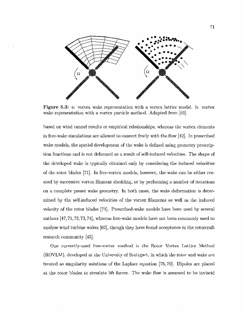
71
Figure 5.3: a: vortex wake representation with a vortex lattice model, b: vortex wake representation with a vortex particle method. Adapted from [45]
based on wind tunnel results or empirical relationships, whereas the vortex elements
in free-wake simulations are allowed to convect freely with the flow [42]. In prescribed
wake models, the spatial development of the wake is defined using geometry prescrip
tion functions and is not deformed as a result of self-induced velocities. The shape of
the developed wake is typically obtained only by considering the induced velocities
of the rotor blades [71]. In free-vortex models, however, the wake can be either cre
ated by successive vortex filament shedding, or by performing a number of iterations
on a complete preset wake geometry. In both cases, the wake deformation is deter
mined by the self-induced velocities of the vortex filaments as well as the induced
velocity of the rotor blades [71]. Prescribed-wake models have been used by several
authors [47,71,72,73,74], whereas free-wake models have not been commonly used to
analyse wind turbine wakes [62], though they have found acceptance in the rotorcraft
research community [45].
One currently-used free-vortex method is the Rotor Vortex Lattice Method
(ROVLM), developed at the University of Stuttgart, in which the rotor and wake are
treated as singularity solutions of the Laplace equation [75,76]. Dipoles are placed
at the rotor blades to simulate lift forces. The wake flow is assumed to be inviscid
72
and irrotational. Vorticity is shed into the wake as a spanwise series of panels from
the trailing edge, where the amount of shed vorticity is determined by the Kutta
condition [25]. In each time step, a new portion of the wake is created and convected
downstream. The wake deformation is determined by multiplying the wake panel
velocities with the time step and a simplified wake transport model is used for the
far wake [75]. ROVLM was used in a study by Whale et al in 2000 to experimentally
and numerically study the vortex structure of a model turbine in a wind tunnel [76].
It was found that the numerical results underpredicted the wake expansion that was
visible in the experiment. Additionally, ROVLM overpredicted the strength of the
shed vortices at the blade root, a problem that the authors attributed to the stall
model that was included in the code [76].
In 2003, Duque et al tested a vortex lattice code, CAMRAD II, against the NREL's
measured data [77]. CAMRAD II was originally developed for rotorcraft and has been
modified for horizontal axis wind turbines and consists of a vortex lattice with a free-
wake model. The solver requires 2D lift and drag data, corrected for stall delay
effects caused by the effect of the Coriolis force effect on the spanwise momentum in
the boundary layer. Results for CAMRAD II with a stall delay model were within
10% of the measured power until the freestream velocity increased beyond 15 m/s,
after which a large over prediction of power was observed, increasing to an error of
50% [77].
A more recently developed free-wake vortex code is that developed at the Uni
versity of Maryland by Gupta and Leishman [36]. Each blade is modeled using a
Weissinger-L lifting surface model, which is a single panel lifting surface. The blades
are separated into a number of spanwise segments over which bound circulation and
lift are constant. The near wake is truncated after an angular rotation of 30 degrees
and a single vortex filament is then trailed from the tip of each blade by assuming
that the bound vorticity rolls up into the tip vortex. The results of this work have
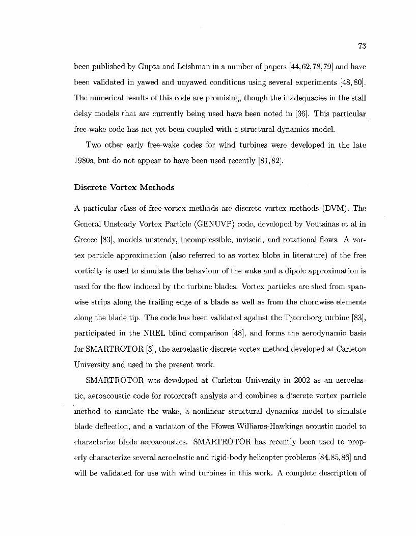
73
been published by Gupta and Leishman in a number of papers [44,62,78,79] and have
been validated in yawed and unyawed conditions using several experiments [48,80].
The numerical results of this code are promising, though the inadequacies in the stall
delay models that are currently being used have been noted in [36]. This particular
free-wake code has not yet been coupled with a structural dynamics model.
Two other early free-wake codes for wind turbines were developed in the late
1980s, but do not appear to have been used recently [81,82].
Discrete Vortex Methods
A particular class of free-vortex methods are discrete vortex methods (DVM). The
General Unsteady Vortex Particle (GENUVP) code, developed by Voutsinas et al in
Greece [83], models unsteady, incompressible, inviscid, and rotational flows. A vor
tex particle approximation (also referred to as vortex blobs in literature) of the free
vorticity is used to simulate the behaviour of the wake and a dipole approximation is
used for the flow induced by the turbine blades. Vortex particles are shed from span-
wise strips along the trailing edge of a blade as well as from the chordwise elements
along the blade tip. The code has been validated against the Tjaereborg turbine [83],
participated in the NREL blind comparison [48], and forms the aerodynamic basis
for SMARTROTOR [3], the aeroelastic discrete vortex method developed at Carleton
University and used in the present work.
SMARTROTOR was developed at Carleton University in 2002 as an aeroelas
tic, aeroacoustic code for rotorcraft analysis and combines a discrete vortex particle
method to simulate the wake, a nonlinear structural dynamics model to simulate
blade deflection, and a variation of the Ffowcs Williams-Hawkings acoustic model to
characterize blade aeroacoustics. SMARTROTOR has recently been used to prop
erly characterize several aeroelastic and rigid-body helicopter problems [84,85,86] and
will be validated for use with wind turbines in this work. A complete description of
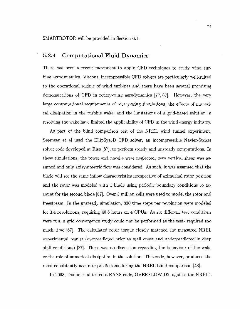
74
SMARTROTOR will be provided in Section 6.1.
5.2.4 Computational Fluid Dynamics
There has been a recent movement to apply CFD techniques to study wind tur
bine aerodynamics. Viscous, incompressible CFD solvers are particularly well-suited
to the operational regime of wind turbines and there have been several promising
demonstrations of CFD in rotary-wing aerodynamics [77,87]. However, the very
large computational requirements of rotary-wing simulations, the effects of numeri
cal dissipation in the turbine wake, and the limitations of a grid-based solution in
resolving the wake have limited the applicability of CFD in the wind energy industry.
As part of the blind comparison test of the NREL wind tunnel experiment,
S0rensen et al used the EllipSys3D CFD solver, an incompressible Navier-Stokes
solver code developed at Ris0 [87], to perform steady and unsteady computations. In
these simulations, the tower and nacelle were neglected, zero vertical shear was as
sumed and only axisymmetric flow was considered. As such, it was assumed that the
blade will see the same inflow characteristics irrespective of azimuthal rotor position
and the rotor was modeled with 1 blade using periodic boundary conditions to ac
count for the second blade [87]. Over 3 million cells were used to model the rotor and
freestream. In the unsteady simulation, 830 time steps per revolution were modeled
for 3.4 revolutions, requiring 40.8 hours on 4 CPUs. As six different test conditions
were run, a grid convergence study could not be performed as the tests required too
much time [87]. The calculated rotor torque closely matched the measured NREL
experimental results (overpredicted prior to stall onset and underpredicted in deep
stall conditions) [87]. There was no discussion regarding the behaviour of the wake
or the role of numerical dissipation in the solution. This code, however, produced the
most consistently accurate predictions during the NREL blind comparison [48].
In 2003, Duque et al tested a RANS code, OVERFLOW-D2, against the NREL's
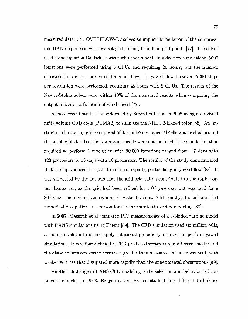
75
measured data [77]. 0VERFL0W-D2 solves an implicit formulation of the compress
ible RANS equations with overset grids, using 11 million grid points [77]. The solver
used a one equation Baldwin-Barth turbulence model. In axial flow simulations, 5000
iterations were performed using 8 CPUs and requiring 26 hours, but the number
of revolutions is not presented for axial flow. In yawed flow however, 7200 steps
per revolution were performed, requiring 48 hours with 8 CPUs. The results of the
Navier-Stokes solver were within 10% of the measured results when comparing the
output power as a function of wind speed [77].
A more recent study was performed by Sezer-Uzol et al in 2006 using an inviscid
finite volume CFD code (PUMA2) to simulate the NREL 2-bladed rotor [88]. An un
structured, rotating grid composed of 3.6 million tetrahedral cells was meshed around
the turbine blades, but the tower and nacelle were not modeled. The simulation time
required to perform 1 revolution with 90,000 iterations ranged from 1.7 days with
128 processors to 15 days with 16 processors. The results of the study demonstrated
that the tip vortices dissipated much too rapidly, particularly in yawed flow [88]. It
was suspected by the authors that the grid orientation contributed to the rapid vor
tex dissipation, as the grid had been refined for a 0° yaw case but was used for a
30 ° yaw case in which an asymmetric wake develops. Additionally, the authors cited
numerical dissipation as a reason for the inaccurate tip vortex modeling [88].
In 2007, Massouh et al compared PIV measurements of a 3-bladed turbine model
with RANS simulations using Fluent [89]. The CFD simulation used six million cells,
a sliding mesh and did not apply rotational periodicity in order to perform yawed
simulations. It was found that the CFD-predicted vortex core radii were smaller and
the distance between vortex cores was greater than measured in the experiment, with
weaker vortices that dissipated more rapidly than the experimental observations [89].
Another challenge in RANS CFD modeling is the selection and behaviour of tur
bulence models. In 2003, Benjanirat and Sankar studied four different turbulence
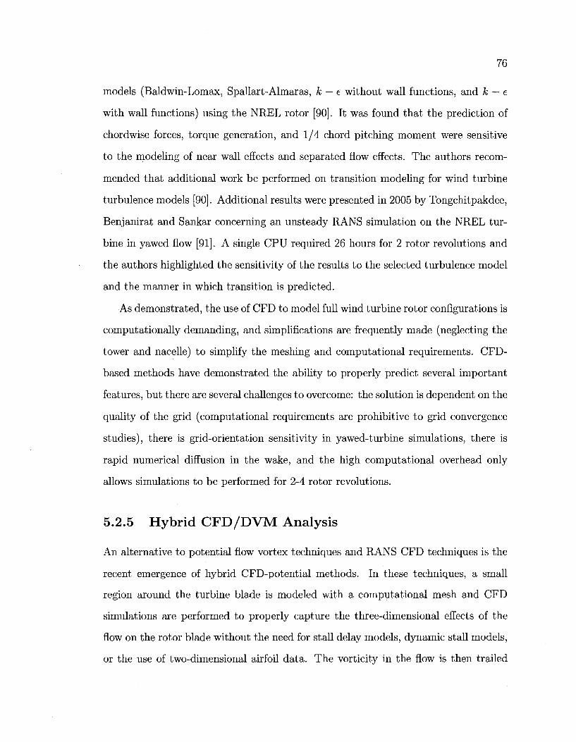
76
models (Baldwin-Lomax, Spallart-Almaras, k — e without wall functions, and k — e
with wall functions) using the NREL rotor [90]. It was found that the prediction of
chordwise forces, torque generation, and 1/4 chord pitching moment were sensitive
to the modeling of near wall effects and separated flow effects. The authors recom
mended that additional work be performed on transition modeling for wind turbine
turbulence models [90]. Additional results were presented in 2005 by Tongchitpakdee,
Benjanirat and Sankar concerning an unsteady RANS simulation on the NREL tur
bine in yawed flow [91]. A single CPU required 26 hours for 2 rotor revolutions and
the authors highlighted the sensitivity of the results to the selected turbulence model
and the manner in which transition is predicted.
As demonstrated, the use of CFD to model full wind turbine rotor configurations is
computationally demanding, and simplifications are frequently made (neglecting the
tower and nacelle) to simplify the meshing and computational requirements. CFD-
based methods have demonstrated the ability to properly predict several important
features, but there are several challenges to overcome: the solution is dependent on the
quality of the grid (computational requirements are prohibitive to grid convergence
studies), there is grid-orientation sensitivity in yawed-turbine simulations, there is
rapid numerical diffusion in the wake, and the high computational overhead only
allows simulations to be performed for 2-4 rotor revolutions.
5.2.5 Hybrid CFD/DVM Analysis
An alternative to potential flow vortex techniques and RANS CFD techniques is the
recent emergence of hybrid CFD-potential methods. In these techniques, a small
region around the turbine blade is modeled with a computational mesh and CFD
simulations are performed to properly capture the three-dimensional effects of the
flow on the rotor blade without the need for stall delay models, dynamic stall models,
or the use of two-dimensional airfoil data. The vorticity in the flow is then trailed
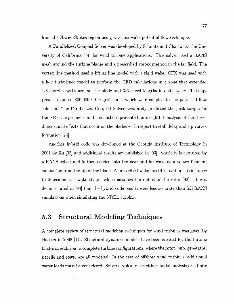
77
from the Navier-Stokes region using a vortex-wake potential flow technique.
A Parallelized Coupled Solver was developed by Schmitz and Chattot at the Uni
versity of California [74] for wind turbine applications. This solver used a RANS
mesh around the turbine blades and a prescribed vortex method in the far field. The
vortex line method used a lifting line model with a rigid wake. CFX was used with
a k-u> turbulence model to perform the CFD calculations in a zone that extended
1-3 chord lengths around the blade and 3-6 chord lengths into the wake. This ap
proach required 800,000 CFD grid nodes which were coupled to the potential flow
solution. The Parallelized Coupled Solver accurately predicted the peak torque for
the NREL experiment and the authors presented an insightful analysis of the three-
dimensional effects that occur on the blades with respect to stall delay and tip vortex
formation [74].
Another hybrid code was developed at the Georgia Institute of Technology in
2001 by Xu [92] and additional results are published in [93]. Vorticity is captured by
a RANS solver and is then carried into the near and far wake as a vortex filament
emanating from the tip of the blade. A prescribed wake model is used in this instance
to determine the wake shape, which assumes the radius of the rotor [92]. It was
demonstrated in [93] that the hybrid code results were less accurate than full RANS
simulations when simulating the NREL turbine.
5.3 Structural Modeling Techniques
A complete review of structural modeling techniques for wind turbines was given by
Hansen in 2006 [47]. Structural dynamics models have been created for the turbine
blades in addition to complete turbine configurations, where the rotor, hub, generator,
nacelle and tower are all modeled. In the case of offshore wind turbines, additional
water loads must be considered. Solvers typically use either modal analysis or a finite
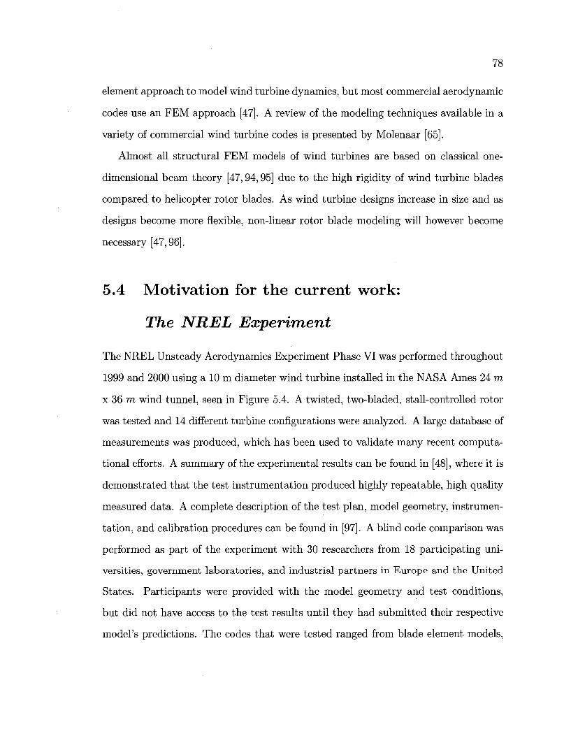
78
element approach to model wind turbine dynamics, but most commercial aerodynamic
codes use an FEM approach [47]. A review of the modeling techniques available in a
variety of commercial wind turbine codes is presented by Molenaar [65].
Almost all structural FEM models of wind turbines are based on classical one-
dimensional beam theory [47,94,95] due to the high rigidity of wind turbine blades
compared to helicopter rotor blades. As wind turbine designs increase in size and as
designs become more flexible, non-linear rotor blade modeling will however become
necessary [47,96].
5.4 Motivation for the current work:
The NREL Experiment
The NREL Unsteady Aerodynamics Experiment Phase VI was performed throughout
1999 and 2000 using a 10 m diameter wind turbine installed in the NASA Ames 24 m
x 36 m wind tunnel, seen in Figure 5.4. A twisted, two-bladed, stall-controlled rotor
was tested and 14 different turbine configurations were analyzed. A large database of
measurements was produced, which has been used to validate many recent computa
tional efforts. A summary of the experimental results can be found in [48], where it is
demonstrated that the test instrumentation produced highly repeatable, high quality
measured data. A complete description of the test plan, model geometry, instrumen
tation, and calibration procedures can be found in [97]. A blind code comparison was
performed as part of the experiment with 30 researchers from 18 participating uni
versities, government laboratories, and industrial partners in Europe and the United
States. Participants were provided with the model geometry and test conditions,
but did not have access to the test results until they had submitted their respective
model's predictions. The codes that were tested ranged from blade element models,
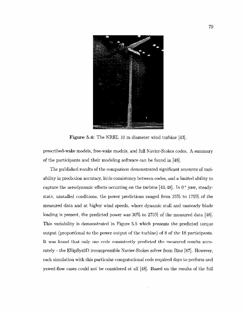
79
Figure 5.4: The NREL 10 m diameter wind turbine [43].
prescribed-wake models, free-wake models, and full Navier-Stokes codes. A summary
of the participants and their modeling software can be found in [48].
The published results of the comparison demonstrated significant amounts of vari
ability in prediction accuracy, little consistency between codes, and a limited ability to
capture the aerodynamic effects occurring on the turbine [43,48]. In 0° yaw, steady-
state, unstalled conditions, the power predictions ranged from 25% to 175% of the
measured data and at higher wind speeds, where dynamic stall and unsteady blade
loading is present, the predicted power was 30% to 275% of the measured data [48].
This variability is demonstrated in Figure 5.5 which presents the predicted torque
output (proportional to the power output of the turbine) of 8 of the 18 participants.
It was found that only one code consistently predicted the measured results accu
rately - the EllipSys3D incompressible Navier-Stokes solver from Ris0 [87]. However,
each simulation with this particular computational code required days to perform and
yawed-flow cases could not be considered at all [48]. Based on the results of the full
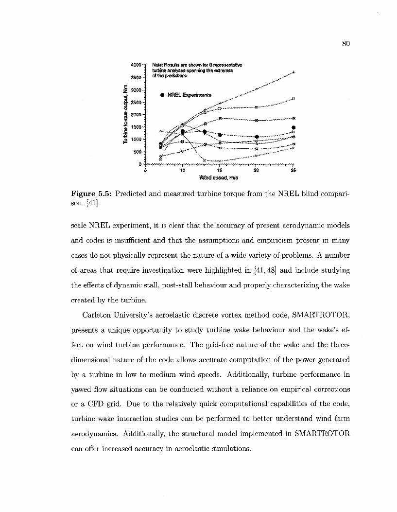
80
4060 -i Note: Rfssufls «re shown for 8 wpteserttettv* turtttw ar»lys«t spanning tt» «trert»$ of tt» predictions 3S0O'
E as 3000-
JL 2500-
S 2000-
er I tsso-3 I 1000
^
NREL Experiments
j ^ " " ^
^'^
^ ^ ^ — —
/A
• S « . \ ™ ^^^^^^""^"^ifttssC^^XHt*^^
*«JB*~
...( ... - y . ^ . — p . . p T (, - f ; ; ^ - ^ — ^ — ^ - v j y — V//y/y|-
10 16 WW speed, m/s
m 25
Figure 5.5: Predicted and measured turbine torque from the NREL blind comparison. [41].
scale NREL experiment, it is clear that the accuracy of present aerodynamic models
and codes is insufficient and that the assumptions and empiricism present in many
cases do not physically represent the nature of a wide variety of problems. A number
of areas that require investigation were highlighted in [41,48] and include studying
the effects of dynamic stall, post-stall behaviour and properly characterizing the wake
created by the turbine.
Carleton University's aeroelastic discrete vortex method code, SMARTROTOR,
presents a unique opportunity to study turbine wake behaviour and the wake's ef
fect on wind turbine performance. The grid-free nature of the wake and the three-
dimensional nature of the code allows accurate computation of the power generated
by a turbine in low to medium wind speeds. Additionally, turbine performance in
yawed flow situations can be conducted without a reliance on empirical corrections
or a CFD grid. Due to the relatively quick computational capabilities of the code,
turbine wake interaction studies can be performed to better understand wind farm
aerodynamics. Additionally, the structural model implemented in SMARTROTOR
can offer increased accuracy in aeroelastic simulations.
Chapter 6
Aerodynamic and Aeroelastic Theory in
SMARTROTOR
SMARTROTOR is a state-of-the-art three-dimensional aeroelastic code developed
specifically for rotary-wing applications. Its aerodynamic model is based on a discrete-
vortex method called GENUVP while the structural model is based on an implemen
tation of Hodges' nonlinear beam model for rotorcraft. A summary of the theory for
these two models will be reviewed in this chapter.
6.1 Aerodynamic Model
The aerodynamic component of SMARTROTOR is the GENeral Unsteady Vortex
Particle (GENUVP) software originally developed by Voutsinas et al at the National
Technical University of Athens [83]. GENUVP uses an unsteady panel method cou
pled to a discrete vortex particle method to resolve the rotor blade and wake aerody
namics.
81
82
6.1.1 GENUVP Theory
A detailed description of the theory implemented in GENUVP can be found in [83,
98,99,100], but the the theory will be summarized in this section for completeness.
The theory for aerodynamic modeling in GENUVP is based on the Helmholtz de
composition, or vorticity transport theorem. The Helmholtz decomposition states
that any vector field can be written as the sum of a solenoidal (rotational, or
divergence-free) and lamellar (irrotational, or curl-free) vector [101]. The Helmholtz
decomposition of an arbitrary velocity field u is expressed as
u^v + Va + V x p (6.1)
where v is the harmonic vector field, a represents a scalar potential, and j3 represents
a vector potential. In the context of a wind turbine, the irrotational component
of the flow represents the influence due to the solid boundaries and the rotational
component of the flow represents the influence of the wake. The velocity field around
a helicopter or wind turbine can be represented with the Helmholtz decomposition as
U yX, t) = Uextemal \%i ") * Usoiid yX, t) + linear—wake {%> Z) -\- Ufar—waice yX, t) (y-^J
where x and t are the position and time, respectively, of the velocity u(x,t) in a
domain D. The irrotational component of the flow in Equation 6.2 is composed
of the the prescribed external velocity field, uexternah the velocity field due to the
influence of solid bodies (such as the rotor blades, the nacelle, or tower), usoud, and
the velocity induced by the near-wake of the lifting surface, unear-wake- The rotational
component of the flow is represented by the induced velocity due to the far-wake of
the rotor blades, described in Equation 6.2 by w/ar-wafce-
83
In GENUVP, singularity distributions are denned on all solid surfaces and the near
wake, whereas the far-wake behind the lifting surface is represented with free-vortex
particles [98]. The far wake velocity, Ufar-wake, induced at a location in space (x) by
the vorticity of a particle (u) located at a point (x0) is given by the Biot-Savart law,
as seen in Equation 6.3.
Ufar-wake {X, t) = / — — — 3 dD ( 6 .3 ) J 47r\x — x0\
Dw{t)
The far wake velocity described by Equation 6.3 can be solved with vortex methods
that describe the vorticity in the field [3]. As such, Equation 6.2 can be solved
using a panel method for the uaoiid and unear^wake terms and a vortex method for
Ufar-wake- As the fluid is inviscid, there is no automatic link between the irrotational
and rotational components of flow [98]. The panel method and the vortex method are
coupled at the interface between the near-wake and far-wake by enforcing the Kutta
condition at the near wake.
6.1.2 Panel Method - Solving for usoM and unear-wake
A panel method was implemented in GENUVP based on the work of Hess [102] in
order to determine the induced velocity in the flowfield from solid lifting and non-
lifting bodies. Dipole distributions are used to generate lift on solid boundaries and
surface vorticity on the near wake sheets, whereas sources are used to account for the
thickness of lifting and non-lifting bodies. This can be illustrated by considering a
body with a surface S in an incompressible, inviscid flowfield. The continuity equation
in an inviscid incompressible flowfield reduces to the Laplace equation as described
by Equation 6.4, where 0 is the velocity scalar potential.
vV = o (6.4)
84
The solution for the velocity potential must satisfy the condition of non-penetration
of solid boundaries and the condition of regularity, as described by Equations 6.5 and
6.6, respectively. The non-penetration boundary condition results in tangential flow
at the surface and the condition of regularity ensures that the velocity approaches
the freestream speed at infinity.
V0 • n\s = d0 dn
= (uext • n - F)s (6.5) s
IWL - 0 (6.6)
In Equation 6.5, n is the unit normal vector on the surface S and F is the local
normal velocity caused by the motion of the body and velocity induced by the far-
wake. Green's identity can be used to write the general solutions of Laplace's equation
(Equation 6.4) as source and dipole distributions over the surfaces of the bodies [3].
The potential caused by a non-lifting body (a turbine tower, nacelle, or hub) is
determined with a continuous source distribution over the surface of the body, whereas
the potential caused by a lifting surface (rotor blade or wing) is determined from a
dipole distribution.
The potential induced at a point P due to the presence of a non-lifting body is
described by Equation 6.7, where a is the local source intensity distribution and r is
the distance to the point P [102].
00-/ a ( i ] AS (6.7) s
A dipole distribution can be used to determine the potential due to thin lifting
body, but a source and dipole distribution must be used to model a thick lifting body.
While GENUVP has the ability to model thin and thick lifting surfaces, only thin
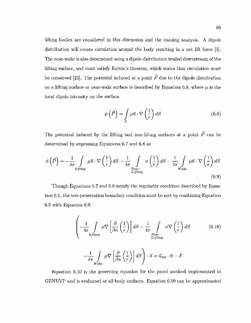
85
lifting bodies are considered in this discussion and the ensuing analysis. A dipole
distribution will create circulation around the body resulting in a net lift force [3].
The near-wake is also determined using a dipole distribution trailed downstream of the
lifting surface, and must satisfy Kelvin's theorem, which states that circulation must
be conserved [23]. The potential induced at a point P due to the dipole distribution
on a lifting surface or near-wake surface is described by Equation 6.8, where fj, is the
local dipole intensity on the surface.
0 00-/ lift • V ( - I dS (6.8)
The potential induced by the lifting and non-lifting surfaces at a point P can be
determined by expressing Equations 6.7 and 6.8 as
lifting N cm-Lifting
Wake
(6.9)
Though Equations 6.7 and 6.8 satisfy the regularity condition described by Equa
tion 6.6, the non-penetration boundary condition must be met by combining Equation
6.5 with Equation 6.9.
(
\
h hv[ti})]dS-i hvi})dS (610) lifting Non-
Lifting
4n J [dn \rJ Wake
dS n = u, ext n
Equation 6.10 is the governing equation for the panel method implemented in
GENUVP and is evaluated at all body surfaces. Equation 6.10 can be approximated
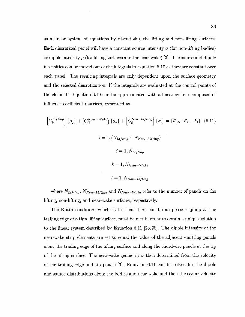
86
as a linear system of equations by discretizing the lifting and non-lifting surfaces.
Each discretized panel will have a constant source intensity a (for non-lifting bodies)
or dipole intensity fi (for lifting surfaces and the near-wake) [3]. The source and dipole
intensities can be moved out of the integrals in Equation 6.10 as they are constant over
each panel. The resulting integrals are only dependent upon the surface geometry
and the selected discretization. If the integrals are evaluated at the control points of
the elements, Equation 6.10 can be approximated with a linear system composed of
influence coefficient matrices, expressed as
{at} = {uext • fU - Fi] (6.11)
% = 1, {NLifting + NNon-Lifting)
J = 1, NLifting
K = 1 i ^Neai—Wake
<• -Lj IV Non—Lifting
where NLifting, NNon_Lifting and NNear_Wake refer to the number of panels on the
lifting, non-lifting, and near-wake surfaces, respectively.
The Kutta condition, which states that there can be no pressure jump at the
trailing edge of a thin lifting surface, must be met in order to obtain a unique solution
to the linear system described by Equation 6.11 [23,98]. The dipole intensity of the
near-wake strip elements are set to equal the value of the adjacent emitting panels
along the trailing edge of the lifting surface and along the chordwise panels at the tip
of the lifting surface. The near-wake geometry is then determined from the velocity
of the trailing edge and tip panels [3]. Equation 6.11 can be solved for the dipole
and source distributions along the bodies and near-wake and then the scalar velocity
/^Lifting Uij M + [c»rr-Wake] w + a Non—Lifting
il
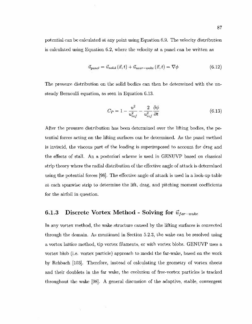
87
potential can be calculated at any point using Equation 6.9. The velocity distribution
is calculated using Equation 6.2, where the velocity at a panel can be written as
V-panel = ^solid (,%•> *) "T" Unem—wake \%"> *) = \ <[> [O.iZ)
The pressure distribution on the solid bodies can then be determined with the un
steady Bernoulli equation, as seen in Equation 6.13.
CP = 1 - - £ — M £ (6-13) Uref Uref9t
After the pressure distribution has been determined over the lifting bodies, the po
tential forces acting on the lifting surfaces can be determined. As the panel method
is inviscid, the viscous part of the loading is superimposed to account for drag and
the effects of stall. An a posteriori scheme is used in GENUVP based on classical
strip theory where the radial distribution of the effective angle of attack is determined
using the potential forces [98]. The effective angle of attack is used in a look-up table
at each spanwise strip to determine the lift, drag, and pitching moment coefficients
for the airfoil in question.
6.1.3 Discrete Vortex Method - Solving for Ufar-wake
In any vortex method, the wake structure caused by the lifting surfaces is convected
through the domain. As mentioned in Section 5.2.3, the wake can be resolved using
a vortex lattice method, tip vortex filaments, or with vortex blobs. GENUVP uses a
vortex blob (i.e. vortex particle) approach to model the far-wake, based on the work
by Rehbach [103]. Therefore, instead of calculating the geometry of vortex sheets
and their doublets in the far wake, the evolution of free-vortex particles is tracked
throughout the wake [98]. A general discussion of the adaptive, stable, convergent
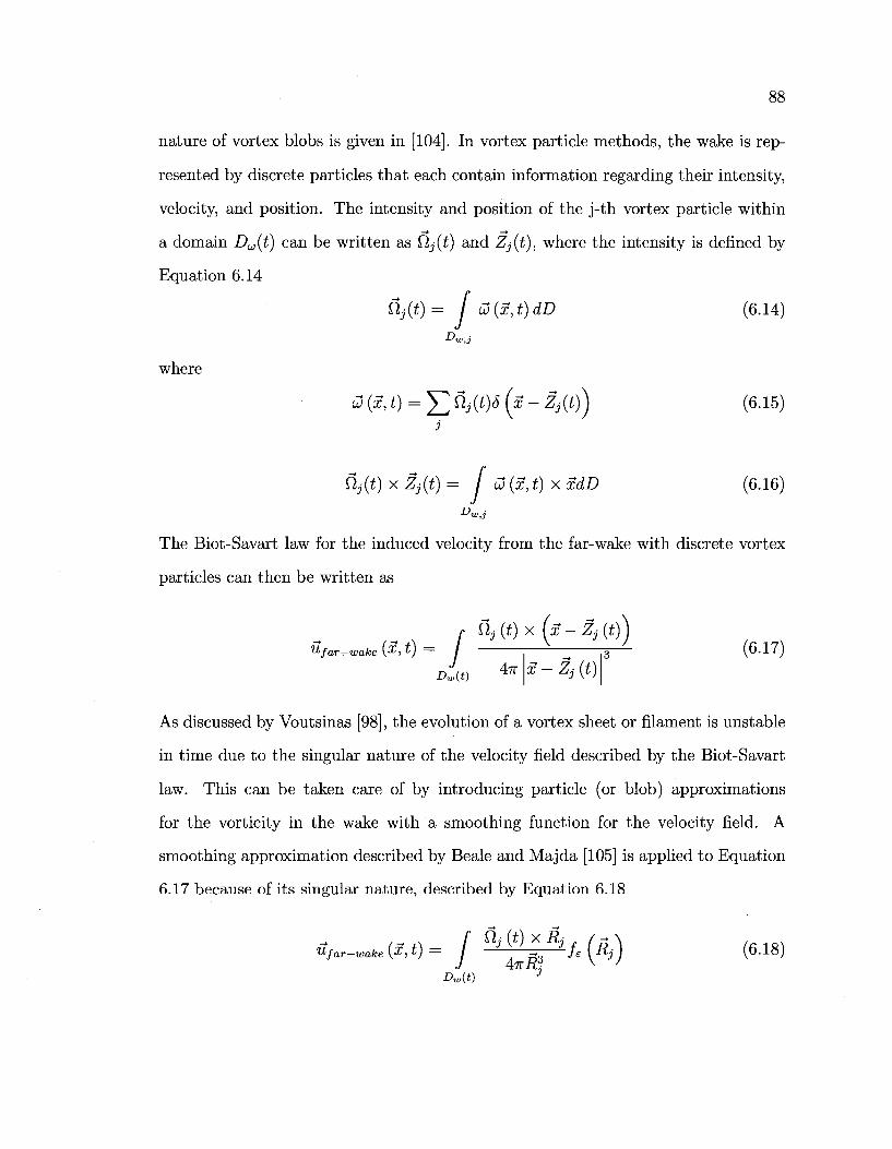
88
nature of vortex blobs is given in [104]. In vortex particle methods, the wake is rep
resented by discrete particles that each contain information regarding their intensity,
velocity, and position. The intensity and position of the j-th vortex particle within
a domain Du(t) can be written as Q,j(t) and Zj(t), where the intensity is defined by
Equation 6.14
fij(t) = J uj{x,t)dD (6.14)
where
j (x, t) = j2 fij(*)<* (^ - 4(*)) (6-15) 3
The Biot-Savart law for the induced velocity from the far-wake with discrete vortex
particles can then be written as
r fij (t) X (x ~ Zj (tj) Ufar-wake(x,t) = / • -^ (6 .17 )
Dw{t) 4 ? r X-Zjit)
As discussed by Voutsinas [98], the evolution of a vortex sheet or filament is unstable
in time due to the singular nature of the velocity field described by the Biot-Savart
law. This can be taken care of by introducing particle (or blob) approximations
for the vorticity in the wake with a smoothing function for the velocity field. A
smoothing approximation described by Beale and Majda [105] is applied to Equation
6.17 because of its singular nature, described by Equation 6.18
ufar-wake(x,t)= J " J ' ^ ^ / « ( ^ ) (6-18) Dw{t) j
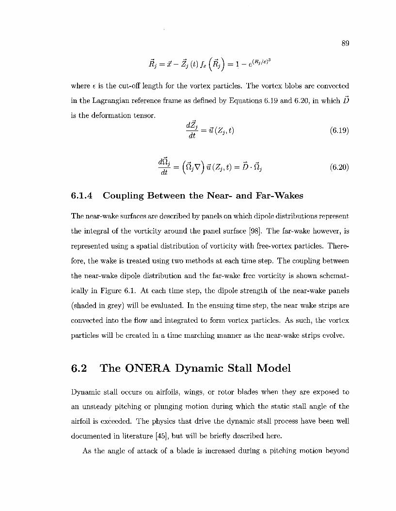
89
Rj = x- Zj (t) U (R^ = 1 - eWe)S
where e is the cut-off length for the vortex particles. The vortex blobs are convected
in the Lagrangian reference frame as defined by Equations 6.19 and 6.20, in which D
is the deformation tensor. —*
^± = u(Z3,t) (6.19)
~dt = (fijV) u (Zj ,t) = D-fij (6.20)
6.1.4 Coupling Between the Near- and Far-Wakes
The near-wake surfaces are described by panels on which dipole distributions represent
the integral of the vorticity around the panel surface [98]. The far-wake however, is
represented using a spatial distribution of vorticity with free-vortex particles. There
fore, the wake is treated using two methods at each time step. The coupling between
the near-wake dipole distribution and the far-wake free vorticity is shown schemat
ically in Figure 6.1. At each time step, the dipole strength of the near-wake panels
(shaded in grey) will be evaluated. In the ensuing time step, the near wake strips are
convected into the flow and integrated to form vortex particles. As such, the vortex
particles will be created in a time marching manner as the near-wake strips evolve.
6.2 The ONERA Dynamic Stall Model
Dynamic stall occurs on airfoils, wings, or rotor blades when they are exposed to
an unsteady pitching or plunging motion during which the static stall angle of the
airfoil is exceeded. The physics that drive the dynamic stall process have been well
documented in literature [45], but will be briefly described here.
As the angle of attack of a blade is increased during a pitching motion beyond
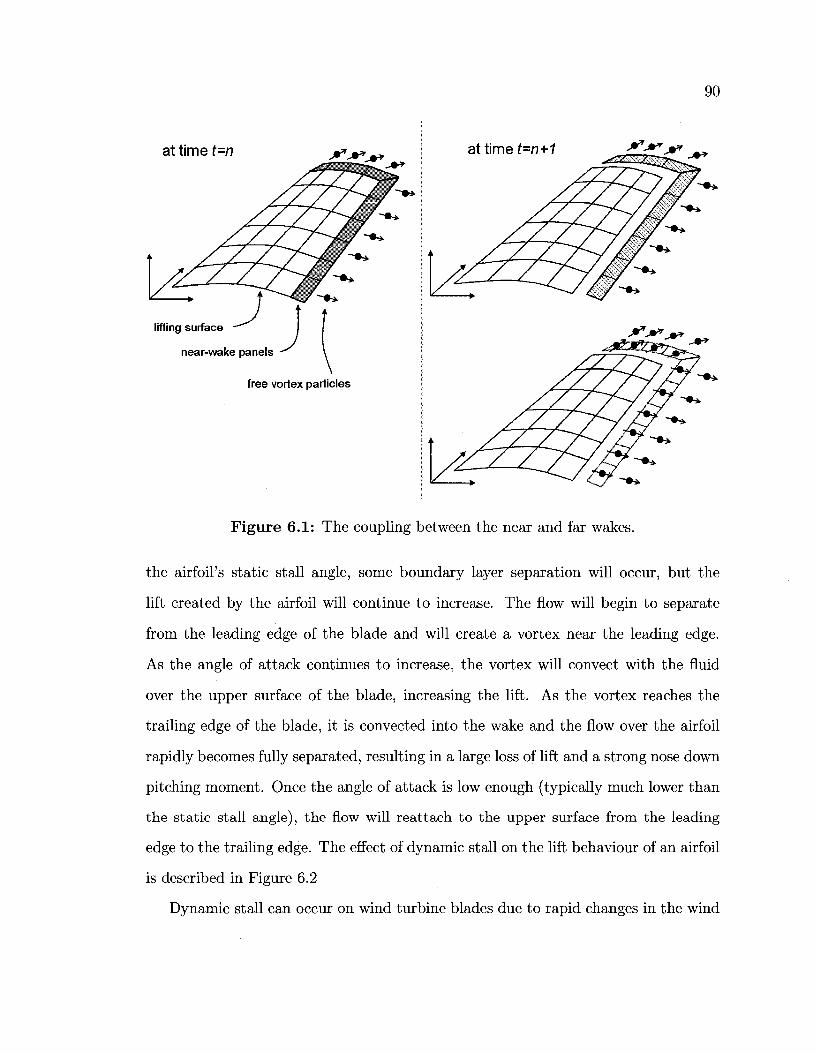
90
Figure 6.1: The coupling between the near and far wakes.
the airfoil's static stall angle, some boundary layer separation will occur, but the
lift created by the airfoil will continue to increase. The flow will begin to separate
from the leading edge of the blade and will create a vortex near the leading edge.
As the angle of attack continues to increase, the vortex will convect with the fluid
over the upper surface of the blade, increasing the lift. As the vortex reaches the
trailing edge of the blade, it is convected into the wake and the flow over the airfoil
rapidly becomes fully separated, resulting in a large loss of lift and a strong nose down
pitching moment. Once the angle of attack is low enough (typically much lower than
the static stall angle), the flow will reattach to the upper surface from the leading
edge to the trailing edge. The effect of dynamic stall on the lift behaviour of an airfoil
is described in Figure 6.2
Dynamic stall can occur on wind turbine blades due to rapid changes in the wind
91
2
1.5
_ 1
0.5
0
-0.5
-5 0 5 10 15 20 a H
Figure 6.2: Effect of dynamic stall on the lift coefficient. Reproduced from [106].
speed, or due to changes in the wind direction, leading to yawed flow situations
where the local angle of attack will change with rotor blade azimuth angle. Though
Navier-Stokes CFD solvers can be used to predict and analyze the effects of dynamic
stall, dynamic stall models are typically used in research or commercial software [45].
Several common stall models are catalogued in [45] and include the ONERA model
[107], the Boeing-Vertol model [108], and the Beddoes-Leishman model [109].
The ONERA model was originally implemented in GENUVP [110] and has been
demonstrated by several authors to adequately capture the lift, moment, and drag
characteristics during dynamic stall on a variety of airfoils [111, 106]. The ONERA
model was originally developed by Iran and Petot in 1981 [107] at the Office Nationale
d'Etudes et de Recherches Aeronautiques (ONERA) in France. The model was de
veloped on the basis of using differential equations to determine the aerodynamic
coefficients for each blade section element during a pitching motion. The original
model was extended by Peters in 1985 [112] to include plunge motions and has been
expressed using either the aerodynamic coefficients, or by the normalized circulation
per unit length [113,114].
1 , , r
dynamic stall
— static stall
J I I L
92
A detailed description of the derivation of the model and the wind tunnel tests
required to characterize and identify the model coefficients can be found in [115].
However, an excellent summary of the original ONERA model in aerodynamic co
efficient form, the extended ONERA model in circulation form, and the suggested
coefficients that can be used to implement the model for a mean airfoil is given by
Petot [111]. A summary of the general differential equations used to model the lift,
moment, and drag coefficients in the ONERA model will be given in this section, and
the discretization, numerical implementation, and the list of the coefficients applied
in SMARTROTOR is presented in Appendix C.
The original version of the ONERA dynamic stall model was originally imple
mented in SMARTROTOR as developed for pitching motions, though it can be used
for more general motions. An aerodynamic coefficient C is expressed as the sum
of two terms in the ONERA dynamic stall model; one term C\ to account for the
attached component of the flow and a second term Ci to account for the separated
flow, as seen in Equation C.l.
C = Ci + C2 (6.21)
C\ represents the load contribution from attached flow and is represented by a
first order differential equation for the lift coefficient as seen in Equation 6.22 and
by an explicit expression for the drag or moment coefficient as expressed in Equation
6.23. The parameter Cun represents the linear portion of the lift, moment, or drag
curve in the absence of stall.
Cx + ACi = XCiin + (As + a) a + so. (6.22)
C\ = Cun + (s + a)a + sa (6.23)
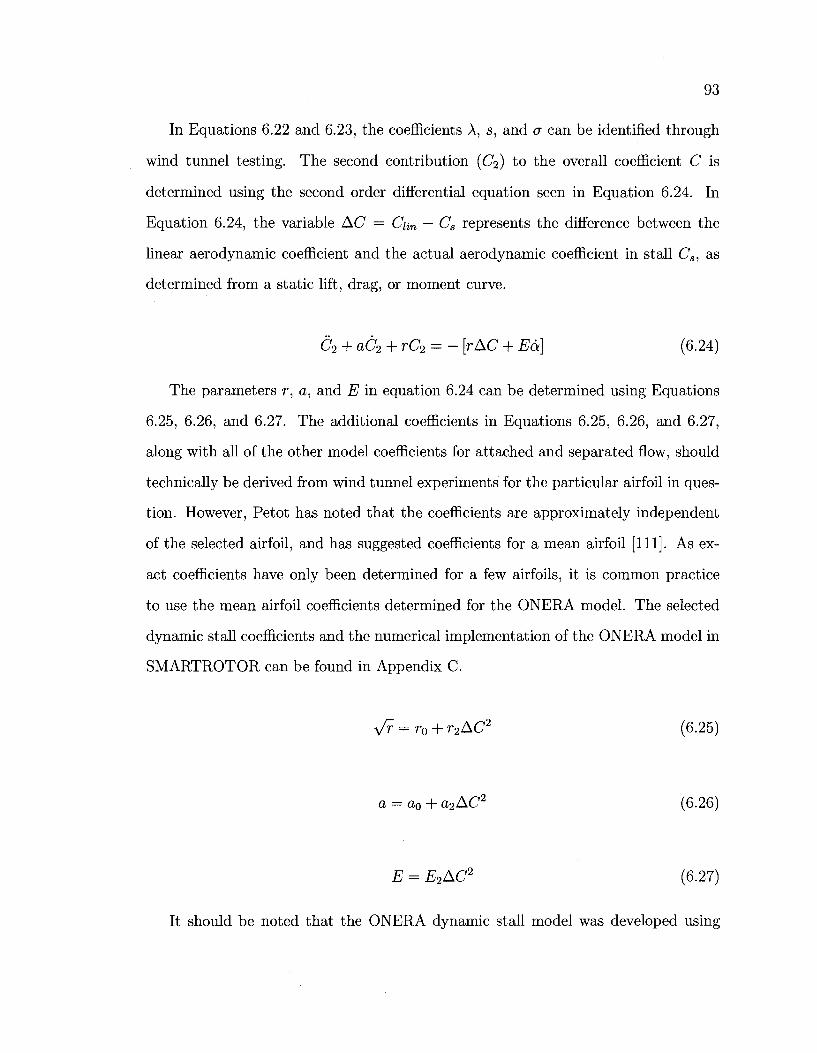
93
In Equations 6.22 and 6.23, the coefficients A, s, and a can be identified through
wind tunnel testing. The second contribution (C2) to the overall coefficient C is
determined using the second order differential equation seen in Equation 6.24. In
Equation 6.24, the variable AC = Cun — Cs represents the difference between the
linear aerodynamic coefficient and the actual aerodynamic coefficient in stall Cs, as
determined from a static lift, drag, or moment curve.
C2 + aC2 + rC2 = - [rAC + Ea] (6.24)
The parameters r, a, and E in equation 6.24 can be determined using Equations
6.25, 6.26, and 6.27. The additional coefficients in Equations 6.25, 6.26, and 6.27,
along with all of the other model coefficients for attached and separated flow, should
technically be derived from wind tunnel experiments for the particular airfoil in ques
tion. However, Petot has noted that the coefficients are approximately independent
of the selected airfoil, and has suggested coefficients for a mean airfoil [111]. As ex
act coefficients have only been determined for a few airfoils, it is common practice
to use the mean airfoil coefficients determined for the ONERA model. The selected
dynamic stall coefficients and the numerical implementation of the ONERA model in
SMARTROTOR can be found in Appendix C.
VF - r0 + r2AC2 (6.25)
a = a0 + a2AC2 (6.26)
E = E2AC2 (6.27)
It should be noted that the ONERA dynamic stall model was developed using
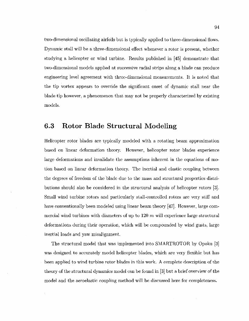
94
two-dimensional oscillating airfoils but is typically applied to three-dimensional flows.
Dynamic stall will be a three-dimensional effect whenever a rotor is present, whether
studying a helicopter or wind turbine. Results published in [45] demonstrate that
two-dimensional models applied at successive radial strips along a blade can produce
engineering level agreement with three-dimensional measurements. It is noted that
the tip vortex appears to override the significant onset of dynamic stall near the
blade tip however, a phenomenon that may not be properly characterized by existing
models.
6.3 Rotor Blade Structural Modeling
Helicopter rotor blades are typically modeled with a rotating beam approximation
based on linear deformation theory. However, helicopter rotor blades experience
large deformations and invalidate the assumptions inherent in the equations of mo
tion based on linear deformation theory. The inertial and elastic coupling between
the degrees of freedom of the blade due to the mass and structural properties distri
butions should also be considered in the structural analysis of helicopter rotors [3].
Small wind turbine rotors and particularly stall-controlled rotors are very stiff and
have conventionally been modeled using linear beam theory [47]. However, large com
mercial wind turbines with diameters of up to 120 m will experience large structural
deformations during their operation, which will be compounded by wind gusts, large
inertial loads and yaw misalignment.
The structural model that was implemented into SMARTROTOR by Opoku [3]
was designed to accurately model helicopter blades, which are very flexible but has
been applied to wind turbine rotor blades in this work. A complete description of the
theory of the structural dynamics model can be found in [3] but a brief overview of the
model and the aeroelastic coupling method will be discussed here for completeness.
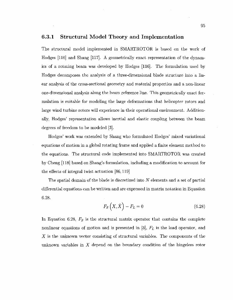
95
6.3.1 Structural Model Theory and Implementation
The structural model implemented in SMARTROTOR is based on the work of
Hodges [116] and Shang [117]. A geometrically exact representation of the dynam
ics of a rotating beam was developed by Hodges [116]. The formulation used by
Hodges decomposes the analysis of a three-dimensional blade structure into a lin
ear analysis of the cross-sectional geometry and material properties and a non-linear
one-dimensional analysis along the beam reference line. This geometrically exact for
mulation is suitable for modeling the large deformations that helicopter rotors and
large wind turbine rotors will experience in their operational environment. Addition
ally, Hodges' representation allows inertial and elastic coupling between the beam
degrees of freedom to be modeled [3].
Hodges' work was extended by Shang who formulated Hodges' mixed variational
equations of motion in a global rotating frame and applied a finite element method to
the equations. The structural code implemented into SMARTROTOR was created
by Cheng [118] based on Shang's formulation, including a modification to account for
the effects of integral twist actuation [86,119]
The spatial domain of the blade is discretized into N elements and a set of partial
differential equations can be written and are expressed in matrix notation in Equation
6.28.
Fs(x,x')-FL = 0 (6.28)
In Equation 6.28, Fs is the structural matrix operator that contains the complete
nonlinear equations of motion and is presented in [3], FL is the load operator, and
X is the unknown vector consisting of structural variables. The components of the
unknown variables in X depend on the boundary condition of the hingeless rotor
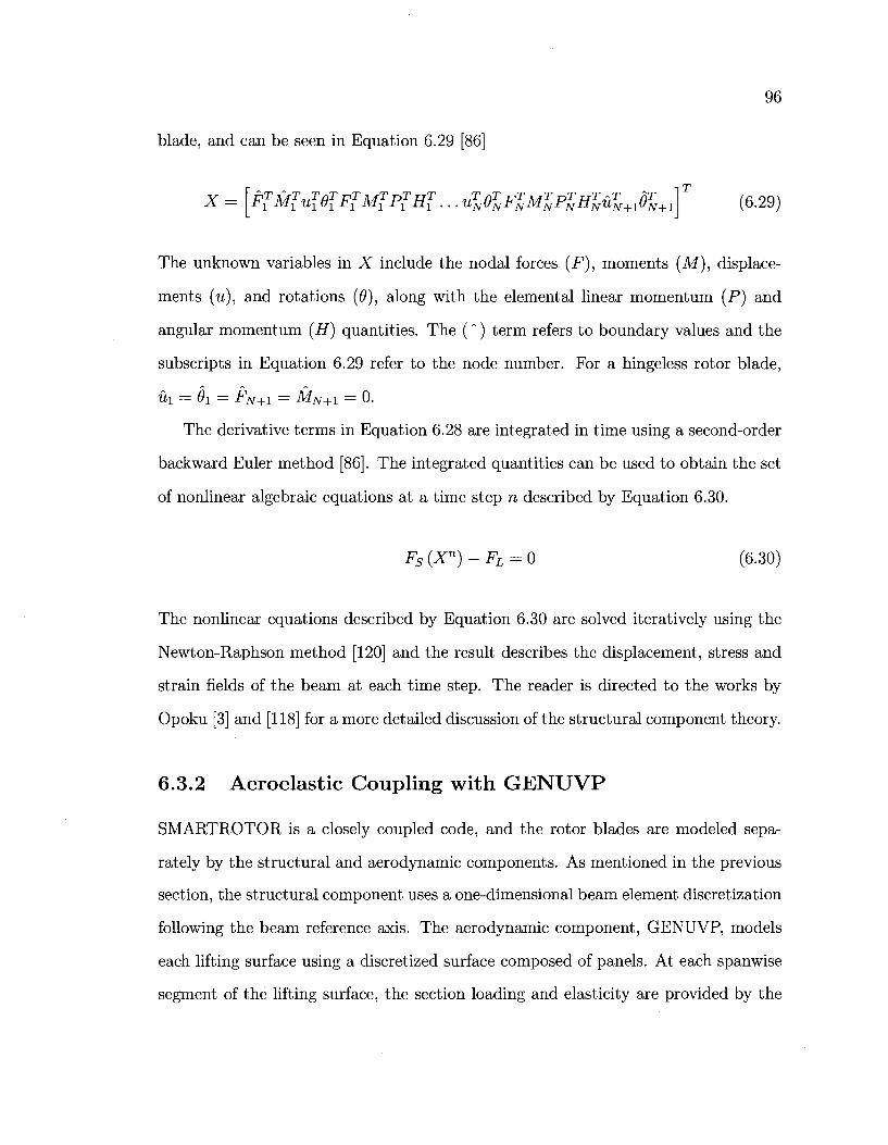
96
blade, and can be seen in Equation 6.29 [86]
'FlMlulQlFlMlP^El... uTNeT
NFlMlPlHTNuT
N+19T
N+A * (6.29) X =
The unknown variables in X include the nodal forces (F), moments (M), displace
ments (u), and rotations (9), along with the elemental linear momentum (P) and
angular momentum (H) quantities. The (") term refers to boundary values and the
subscripts in Equation 6.29 refer to the node number. For a hingeless rotor blade,
«i = 0i = FN+I = MN+I = 0.
The derivative terms in Equation 6.28 are integrated in time using a second-order
backward Euler method [86]. The integrated quantities can be used to obtain the set
of nonlinear algebraic equations at a time step n described by Equation 6.30.
Fs(Xn)-FL = 0 (6.30)
The nonlinear equations described by Equation 6.30 are solved iteratively using the
Newton-Raphson method [120] and the result describes the displacement, stress and
strain fields of the beam at each time step. The reader is directed to the works by
Opoku [3] and [118] for a more detailed discussion of the structural component theory.
6.3.2 Aeroelastic Coupling with GENUVP
SMARTROTOR is a closely coupled code, and the rotor blades are modeled sepa
rately by the structural and aerodynamic components. As mentioned in the previous
section, the structural component uses a one-dimensional beam element discretization
following the beam reference axis. The aerodynamic component, GENUVP, models
each lifting surface using a discretized surface composed of panels. At each spanwise
segment of the lifting surface, the section loading and elasticity are provided by the
97
aerodynamic and structural components, respectively [3]. The aerodynamic compo
nent solves for the potential and viscous loading at each spanwise strip. The spanwise
loading distribution is then transferred by the structural solver to the beam reference
axis and the aeroelastic response of the beam is determined. The elastic deformation
determined by the structural solver is then used to deform the geometry of the panels
on the lifting surface. The plunge, lag, extension, and pitch degrees of freedom are
used for the aeroelastic coupling. The rate of elastic deformation is also determined
and results in an additional lifting surface velocity component F that is accounted
for in the non-penetration boundary condition used by GENUVP (see Equations 6.5
and 6.11).
The aerodynamic and elastic loads and deformations are exchanged at each time
step in SMARTROTOR using an interface routine described by Opoku [3]. The
meshes used for the aerodynamic and structural meshes are coincident in the spanwise
direction of each lifting surface. As such, the width of each structural beam element
is the same as the width of the corresponding spanwise strip of aerodynamic panels.
Additionally, the structural and aerodynamic solvers use the same time step during
simulations. The inputs to the structural model at each spanwise beam element are
the inverse mass and stiffness matrices, where the mass and stiffness matrices are
given by Equations 6.31 and 6.32. The terms mi, m2, and m3 in Equation 6.31 refer
to the directional mass distribution within an element and In , J22, and 33 are the
mass moments of inertia about the x, y and z axes. In the stiffness matrix, EA is
the axial stiffness of the blade, G J is the torsional stiffness, and EIFLAP and EILAG
represent the flapwise and edgewise stiffness terms, respectively.
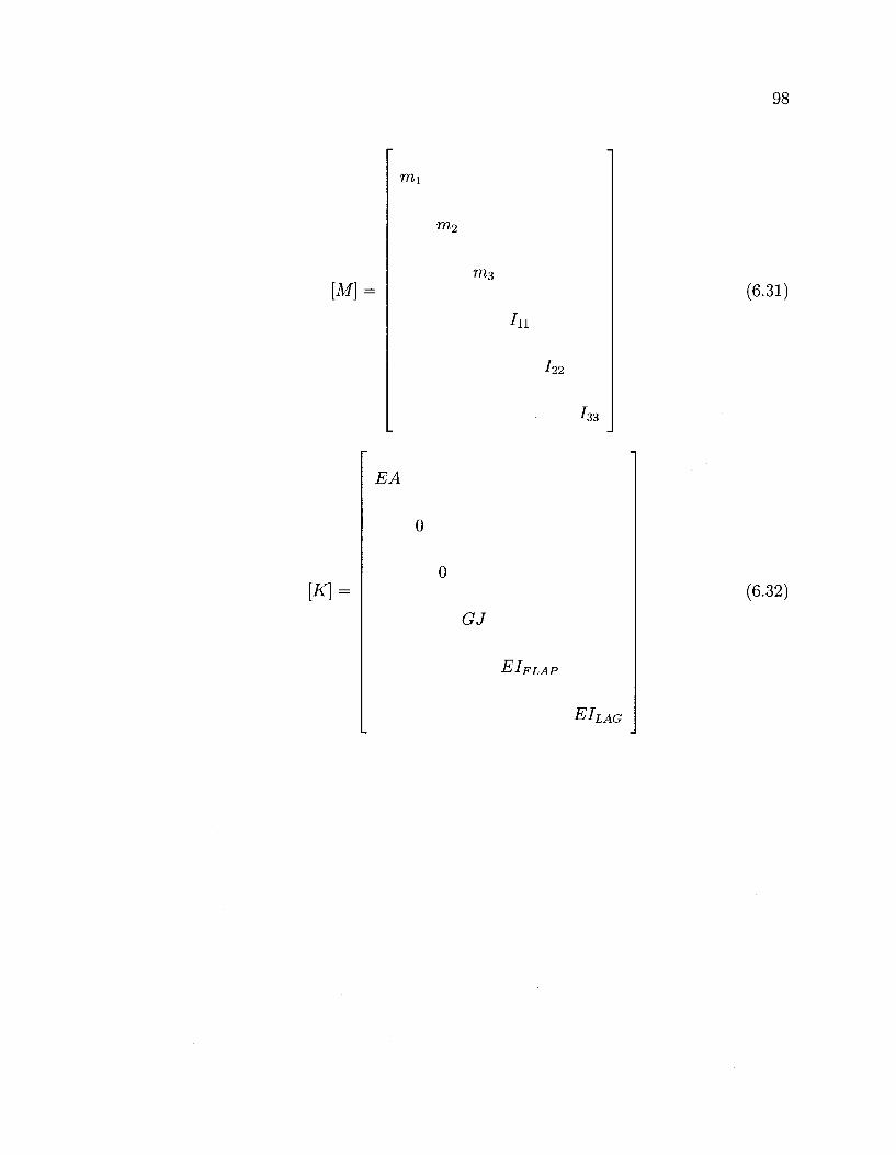
98
[M) =
mx
m2
m3
'11
'22
'33
(6.31)
[K} =
EA
GJ
EI, FLAP
EL LAG
(6.32)
Chapter 7
R e s u l t s
SMARTROTOR was validated as an industrial tool for wind turbine performance
prediction using the National Renewable Energy Laboratory (NREL) 10 m turbine
experiment in a series of simulations.
7.1 Rigid Body Aerodynamic Results
The NREL S809 airfoil was selected for validation as the airfoil has been implemented
on several wind turbine rotors including the NREL experimental turbine. The S809
airfoil was specifically tailored to the requirements of the wind turbine industry and
features a low maximum lift coefficient and gentle stall characteristics. The design,
development, and initial testing of the S809 airfoil is documented in [121] and steady
and unsteady wind tunnel testing of the airfoil can be found in [122]. A cross-
section of the airfoil can be seen in Figure 7.1, in which the mean camber line is
represented with a dashed line. The current version of SMARTROTOR uses a thin
airfoil approximation, where the airfoil is represented by panels mapped onto its mean
camber line.
99
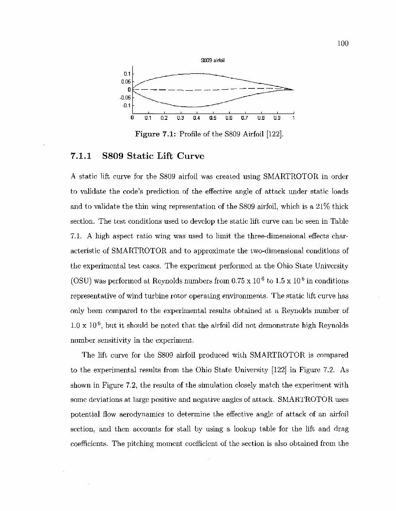
100
S809 airfoil
I i i i i i i i i i i
0 0.1 0.2 0.3 0.4 0.5 0.6 0.7 0.8 0.9 1
Figure 7.1: Profile of the S809 Airfoil [122].
7.1.1 S809 Static Lift Curve
A static lift curve for the S809 airfoil was created using SMARTROTOR in order
to validate the code's prediction of the effective angle of attack under static loads
and to validate the thin wing representation of the S809 airfoil, which is a 21% thick
section. The test conditions used to develop the static lift curve can be seen in Table
7.1. A high aspect ratio wing was used to limit the three-dimensional effects char
acteristic of SMARTROTOR and to approximate the two-dimensional conditions of
the experimental test cases. The experiment performed at the Ohio State University
(OSU) was performed at Reynolds numbers from 0.75 x 10 6 to 1.5 x 10 6 in conditions
representative of wind turbine rotor operating environments. The static lift curve has
only been compared to the experimental results obtained at a Reynolds number of
1.0 x 10 6, but it should be noted that the airfoil did not demonstrate high Reynolds
number sensitivity in the experiment.
The lift curve for the S809 airfoil produced with SMARTROTOR is compared
to the experimental results from the Ohio State University [122] in Figure 7.2. As
shown in Figure 7.2, the results of the simulation closely match the experiment with
some deviations at large positive and negative angles of attack. SMARTROTOR uses
potential flow aerodynamics to determine the effective angle of attack of an airfoil
section, and then accounts for stall by using a lookup table for the lift and drag
coefficients. The pitching moment coefficient of the section is also obtained from the
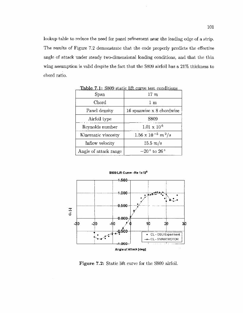
101
lookup table to reduce the need for panel refinement near the leading edge of a strip.
The results of Figure 7.2 demonstrate that the code properly predicts the effective
angle of attack under steady two-dimensional loading conditions, and that the thin
wing assumption is valid despite the fact that the S809 airfoil has a 21% thickness to
chord ratio.
Table 7.1: S809 static lift curve test conditions Span
Chord
Panel density
Airfoil type
Reynolds number
Kinematic viscosity
Inflow velocity
Angle of attack range
17 m
1 m
16 spanwise x 8 chordwise
S809
1.01 x 10⁶
1 . 5 6 x l 0 - 5 m 2 / s
15.5 m/s
-20° to 26°
S809 Lift Curve-Re 1x10⁶
1.500
-4-606-
-0^506-
j * * . - *
/ v. ' l ^ r - " *
0.000 A /
30 •20 / <P 10 2D 3d
^ see-
-1.000
• CL-OSU Experiment
-^-CL-SMARTROTOR
Angle of Attack [deg]
Figure 7.2: Static lift curve for the S809 airfoil.
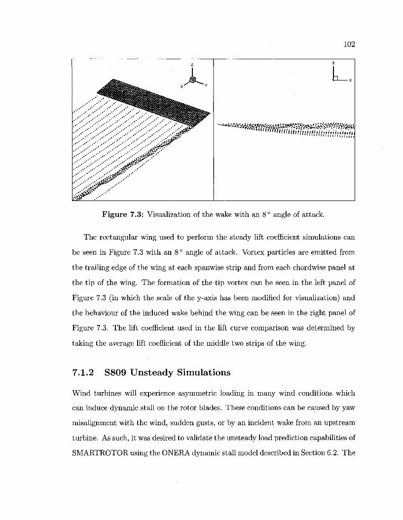
102
Figure 7.3: Visualization of the wake with an 8° angle of attack.
The rectangular wing used to perform the steady lift coefficient simulations can
be seen in Figure 7.3 with an 8 ° angle of attack. Vortex particles are emitted from
the trailing edge of the wing at each spanwise strip and from each chordwise panel at
the tip of the wing. The formation of the tip vortex can be seen in the left panel of
Figure 7.3 (in which the scale of the y-axis has been modified for visualization) and
the behaviour of the induced wake behind the wing can be seen in the right panel of
Figure 7.3. The lift coefficient used in the lift curve comparison was determined by
taking the average lift coefficient of the middle two strips of the wing.
7.1.2 S809 Unsteady Simulations
Wind turbines will experience asymmetric loading in many wind conditions which
can induce dynamic stall on the rotor blades. These conditions can be caused by yaw
misalignment with the wind, sudden gusts, or by an incident wake from an upstream
turbine. As such, it was desired to validate the unsteady load prediction capabilities of
SMARTROTOR using the ONERA dynamic stall model described in Section 6.2. The
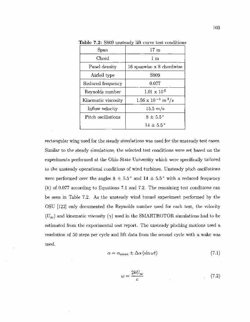
103
Table 7.2; S809 unsteady lift curve test conditions
Span
Chord
Panel density
Airfoil type
Reduced frequency
Reynolds number
Kinematic viscosity
Inflow velocity
Pitch oscillations
17 m
1 m
16 spanwise x 8 chordwise
S809
0.077
1.01 x l O 6
1.56 x 10- 5 m2/s
15.5 m/s
8 ± 5 . 5 °
14 ± 5 . 5 °
rectangular wing used for the steady simulations was used for the unsteady test cases.
Similar to the steady simulations, the selected test conditions were set based on the
experiments performed at the Ohio State University which were specifically tailored
to the unsteady operational conditions of wind turbines. Unsteady pitch oscillations
were performed over the angles 8 ± 5.5° and 14 ± 5.5° with a reduced frequency
(k) of 0.077 according to Equations 7.1 and 7.2. The remaining test conditions can
be seen in Table 7.2. As the unsteady wind tunnel experiment performed by the
OSU [122] only documented the Reynolds number used for each test, the velocity
(t/oo) and kinematic viscosity (7) used in the SMARTROTOR simulations had to be
estimated from the experimental test report. The unsteady pitching motions used a
resolution of 50 steps per cycle and lift data from the second cycle with a wake was
used.
Oi = Olmean ± Ad! ( s in U)t) (7 .1)
to = c
(7.2)
104
An initial simulation was conducted without the ONERA dynamic stall model
to observe how SMARTROTOR predicted the stall hysteresis using only inviscid
potential forces. As expected, the unsteady lift curve shown in Figure 7.4 (with a
dashed line) demonstrates that SMARTROTOR does a poor job of representing the
unsteady behaviour characteristic of dynamic stall without the ONERA model.
The ONERA dynamic stall model has 9 coefficients that describe the attached
flow and separated flow behaviour of the differential equations for lift as discussed in
Section 6.2. The acceptable range for each coefficient in the ONERA dynamic stall
model is presented by Petot in [111] along with coefficients that can be used for a
mean airfoil shape. The mean ONERA coefficients were used to observe how well
the behaviour of the S809 airfoil in dynamic stall was predicted. As seen in Figure
7.4, the original ONERA dynamic stall model poorly captures the stall hysteresis
observed in the experiment. The ONERA model coefficients were originally designed
for helicopter rotors operating conditions and may not be ideally tailored to wind
turbine blade conditions. It was noted in [106] that the coefficients of the Beddoes-
Leishman dynamic stall model had to be modified in order to properly characterize
the behaviour of the S809 airfoil when trying to match the OSU experimental data,
and so it was decided to modify two of the ONERA coefficients that describe the at
tached flow differential equation. The revised coefficients can be found in Appendix
C, and the unsteady S809 lift curve produced with the calibrated ONERA model over
the angles 8 ± 5.5 ° can be seen in Figure 7.5. The ONERA model with the calibrated
coefficients properly characterizes the loading on the wing, but the peak amplitude
of the lift coefficient is lower than the experimental results. Some of this error may
have occurred as many of the simulation parameters had to be estimated based on
the limited information provided in the experimental test report [122]. The dynamic
stall results closely match those obtained by Gupta [36]. A second simulation was
performed over the interval 14 ± 5.5° to observe the behaviour of the calibrated
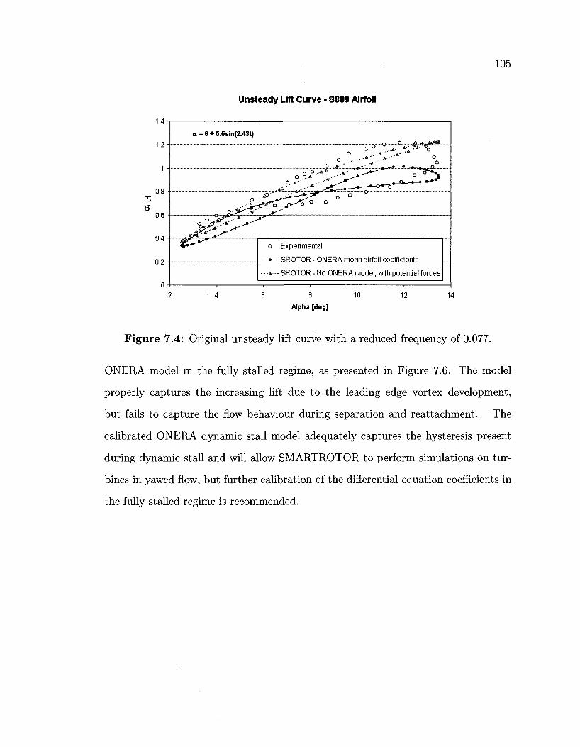
1.4
0.2
Unsteady Lift Curve - S809 Airfoil
ct = 8 + 5.5sin(2.43t)
o Experimental
-*— SROTOR - ONERA mean airfoil coefficients
—»— SROTOR - No ONERA model, with potential forces
10 12 14 Alpha [deg]
105
Figure 7.4: Original unsteady lift curve with a reduced frequency of 0.077.
ONERA model in the fully stalled regime, as presented in Figure 7.6. The model
properly captures the increasing lift due to the leading edge vortex development,
but fails to capture the flow behaviour during separation and reattachment. The
calibrated ONERA dynamic stall model adequately captures the hysteresis present
during dynamic stall and will allow SMARTROTOR to perform simulations on tur
bines in yawed flow, but further calibration of the differential equation coefficients in
the fully stalled regime is recommended.
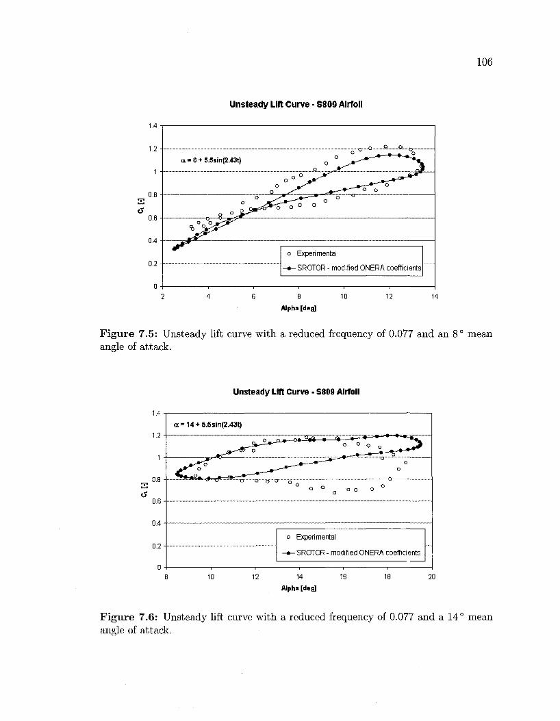
106
Unsteady Lift Curve - S809 Airfoil
1.4
1.2
0.8
o 0.6
0.4
0.2
. ^ o o .
a.= 8 + 5.5sin(2.43t)
o
8 ° ^
o
o 0
o " ^ _ ^ _ ^ b
» ^ ^ * — o
~^W^ *r
1 -1
o Experimental
- • -SR0T0R - modified ONERA coefficients
1 r 1
8 10
Alpha [deg]
12 14
Figure 7.5: Unsteady lift curve with a reduced frequency of 0.077 and an 8° mean angle of attack.
Unsteady Lift Curve - S809 Airfoil
o Experimental
* - SROTOR - modified ONERA coefficients
12 14 1E
Alpha [deg] 20
Figure 7.6: Unsteady lift curve with a reduced frequency of 0.077 and a 14° mean angle of attack.
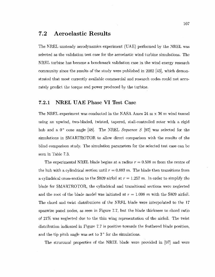
107
7.2 Aeroelastic Results
The NREL unsteady aerodynamics experiment (UAE) performed by the NREL was
selected as the validation test case for the aeroelastic wind turbine simulations. The
NREL turbine has become a benchmark validation case in the wind energy research
community since the results of the study were published in 2002 [43], which demon
strated that most currently available commercial and research codes could not accu
rately predict the torque and power produced by the turbine.
7.2.1 NREL UAE Phase VI Test Case
The NREL experiment was conducted in the NASA Ames 24 m x 36 m wind tunnel
using an upwind, two-bladed, twisted, tapered, stall-controlled rotor with a rigid
hub and a 0° cone angle [48]. The NREL Sequence S [97] was selected for the
simulations in SMARTROTOR to allow direct comparison with the results of the
blind comparison study. The simulation parameters for the selected test case can be
seen in Table 7.3.
The experimental NREL blade begins at a radius r = 0.508 m from the centre of
the hub with a cylindrical section until r = 0.883 m. The blade then transitions from
a cylindrical cross-section to the S809 airfoil at r = 1.257 m. In order to simplify the
blade for SMARTROTOR, the cylindrical and transitional sections were neglected
and the root of the blade model was initiated at r = 1.008 m with the S809 airfoil.
The chord and twist distributions of the NREL blade were interpolated to the 17
spanwise panel nodes, as seen in Figure 7.7, but the blade thickness to chord ratio
of 21% was neglected due to the thin wing representation of the airfoil. The twist
distribution indicated in Figure 7.7 is positive towards the feathered blade position,
and the tip pitch angle was set to 3 ° for the simulations.
The structural properties of the NREL blade were provided in [97] and were
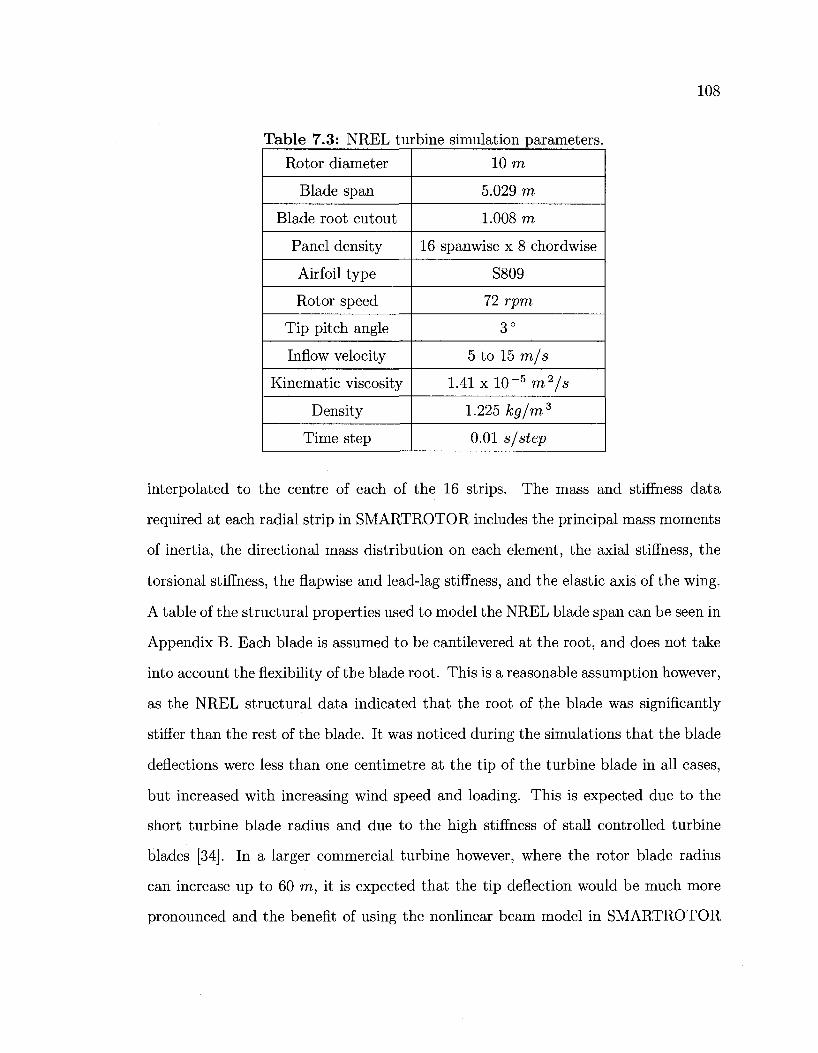
108
Table 7.3: NREL turbine simulation parameters.
Rotor diameter
Blade span
Blade root cutout
Panel density
Airfoil type
Rotor speed
Tip pitch angle
Inflow velocity
Kinematic viscosity
Density
Time step
10 m
5.029 m
1.008 m
16 spanwise x 8 chordwise
S809
72 rpm
3°
5 to 15 m/s
1.41 x 10- 5 m2/s
1.225 kg/m3
0.01 s/step
interpolated to the centre of each of the 16 strips. The mass and stiffness data
required at each radial strip in SMARTROTOR includes the principal mass moments
of inertia, the directional mass distribution on each element, the axial stiffness, the
torsional stiffness, the flapwise and lead-lag stiffness, and the elastic axis of the wing.
A table of the structural properties used to model the NREL blade span can be seen in
Appendix B. Each blade is assumed to be cantilevered at the root, and does not take
into account the flexibility of the blade root. This is a reasonable assumption however,
as the NREL structural data indicated that the root of the blade was significantly
stiffer than the rest of the blade. It was noticed during the simulations that the blade
deflections were less than one centimetre at the tip of the turbine blade in all cases,
but increased with increasing wind speed and loading. This is expected due to the
short turbine blade radius and due to the high stiffness of stall controlled turbine
blades [34]. In a larger commercial turbine however, where the rotor blade radius
can increase up to 60 m, it is expected that the tip deflection would be much more
pronounced and the benefit of using the nonlinear beam model in SMARTROTOR
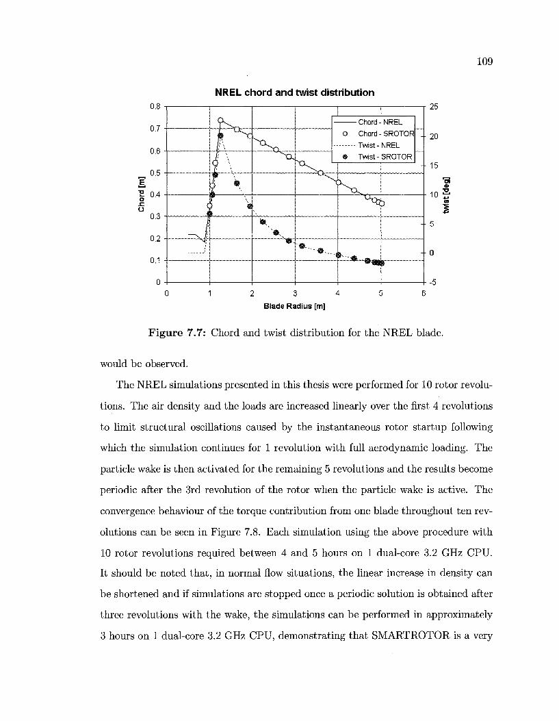
109
NREL chord and twist distribution
n R -
n c _ -> ^
6 c
[ui]p
Cho
r
n i -
n 1 -
0 -
i
-J ~~**$f
f\ Q '
5 *
i •^
^•,,
| |
O Chord -
NREL
SROTOR
NREL
m Twist-SROTOR
"•..
--
--
" ^
" " " • - - m (^"~*.
--
--
2 3 4 Blade Radius [m]
25
20
- 15
10 £•
Figure 7.7: Chord and twist distribution for the NREL blade.
would be observed.
The NREL simulations presented in this thesis were performed for 10 rotor revolu
tions. The air density and the loads are increased linearly over the first 4 revolutions
to limit structural oscillations caused by the instantaneous rotor startup following
which the simulation continues for 1 revolution with full aerodynamic loading. The
particle wake is then activated for the remaining 5 revolutions and the results become
periodic after the 3rd revolution of the rotor when the particle wake is active. The
convergence behaviour of the torque contribution from one blade throughout ten rev
olutions can be seen in Figure 7.8. Each simulation using the above procedure with
10 rotor revolutions required between 4 and 5 hours on 1 dual-core 3.2 GHz CPU.
It should be noted that, in normal flow situations, the linear increase in density can
be shortened and if simulations are stopped once a periodic solution is obtained after
three revolutions with the wake, the simulations can be performed in approximately
3 hours on 1 dual-core 3.2 GHz CPU, demonstrating that SMARTROTOR is a very
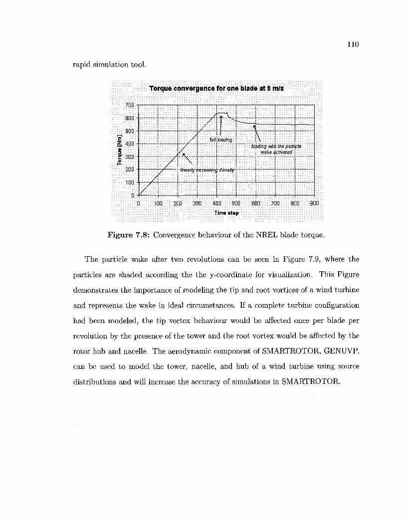
rapid simulation tool.
110
Torque convergence for one blade at 8 m/s
; 700 -i
3 C
D
C
Tor
3 C
IUU -
0-
H •
f:;^V
/
."W\
.*...JS^...
loading
linearly increasing aensiiy
%
\ "•••:• losding wit/} the pMicis
wake activated
0 100 200 300 400 500 600::;;; 700 800 900
Time step :
Figure 7.8: Convergence behaviour of the NREL blade torque.
The particle wake after two revolutions can be seen in Figure 7.9, where the
particles are shaded according the the y-coordinate for visualization. This Figure
demonstrates the importance of modeling the tip and root vortices of a wind turbine
and represents the wake in ideal circumstances. If a complete turbine configuration
had been modeled, the tip vortex behaviour would be affected once per blade per
revolution by the presence of the tower and the root vortex would be affected by the
rotor hub and nacelle. The aerodynamic component of SMARTROTOR, GENUVP,
can be used to model the tower, nacelle, and hub of a wind turbine using source
distributions and will increase the accuracy of simulations in SMARTROTOR.
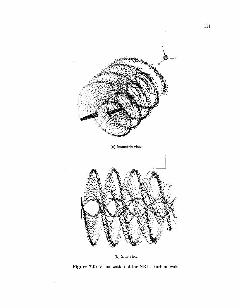
(a) Isometric view.
(b) Side view.
Figure 7.9: Visualization of the NREL turbine wake.
112
The torque produced by the NREL turbine was calculated in SMARTROTOR and
has been superimposed onto the results of the NREL blind comparison study in Figure
7.10. The torque plot was originally published by Leishman [41] and includes results
from 8 of the 18 participants in the NREL blind comparison that are representative
of the extremes predicted by all of the participants. The best prediction of the NREL
power curve was the CFD solution of S0rensen [87] which can be seen in Figure 7.10 as
the line that mimics the experimental data points. Participants in the NREL blind
comparison study were asked to provide results at 7, 10, 13, 15, 20, and 25 m/s,
but additional experimental results were available in 1 m/s intervals from [44] and
added to the original plot from [41] for further validation with SMARTROTOR. The
predicted power output and the predicted turbine thrust predicted are compared to
the NREL experimental results published in [44] in Figures 7.11 and 7.12. As seen
in Figures 7.10 and 7.11, the stall-controlled NREL turbine reaches its rated turbine
power at approximately 10 m/s and the power curve exhibits the wavy behaviour
characteristic of stall-controlled turbines above the rated turbine speed. Above the
rated wind speed, the majority of the turbine blades will be continuously operating in
stalled and deep-stall conditions and the amount of blade stall will govern the output
power.
The errors in the torque and power predictions were within 15% of the experimen
tal data at wind speeds up to and including 10 m/s, and were overpredicted by 35%
to 40% at wind speeds higher than 10 m/s. However, the axial thrust predicted with
SMARTROTOR was within 8% at all simulated wind speeds, indicating that over-
estimation of the radial loading likely contributed to the error in torque and power.
Additionally, overestimation of the effective angle of attack and inadequate character
ization of three-dimensional stall effects over the span of the rotor also contributed to
the observed errors. Blade stall is a three-dimensional phenomenon on wind turbine
rotors and the viscous correction in SMARTROTOR is in effect a two-dimensional
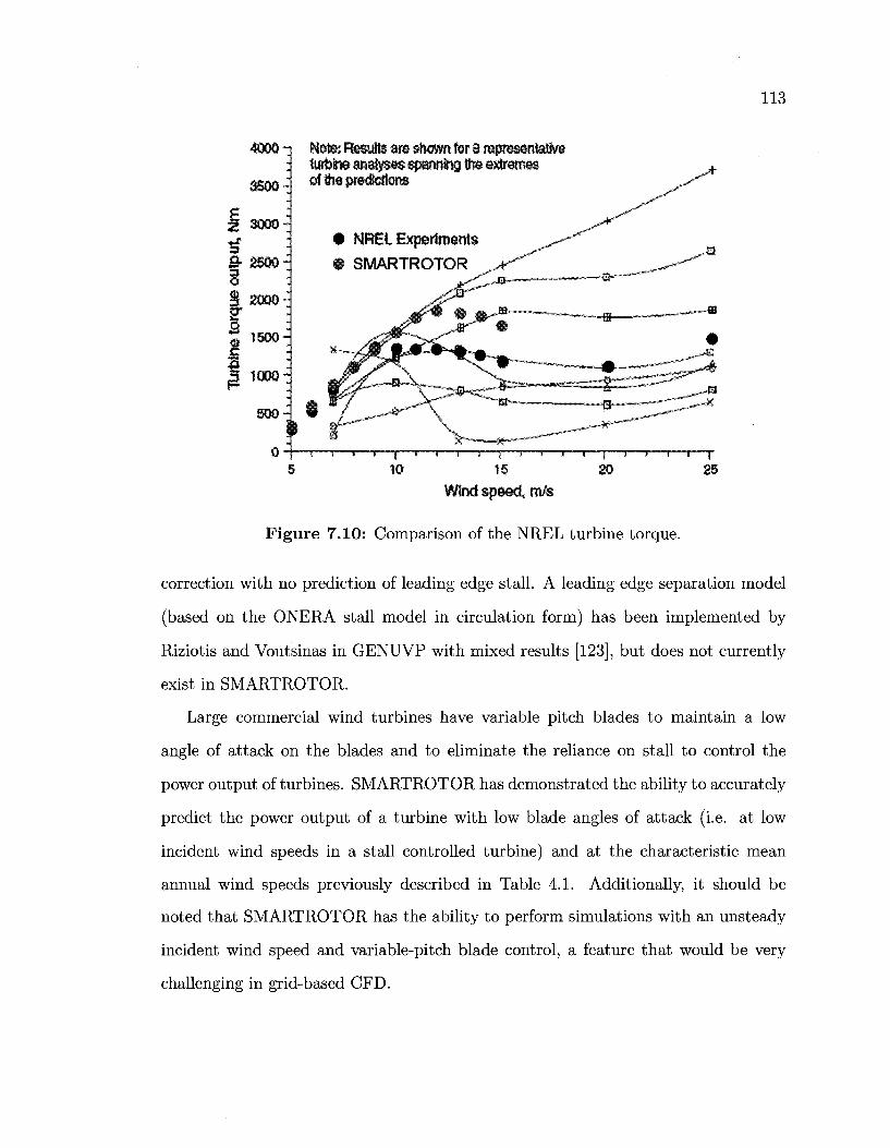
113
4®0 q Note: Results are shown for 8 representative ij turbine angles spannfog the extremes
of the predictions
NREL Experiment
SMARTROTOR
Z WW'
» 2 5 M H 3 O S awH E* o
1 3 1000-
500-H .1 "1 ) % 1 J I 1 1 1 1 1 1 —
10 15 Wtrtd speed, ra/s
20 25
Figure 7.10: Comparison of the NREL turbine torque.
correction with no prediction of leading edge stall. A leading edge separation model
(based on the ONERA stall model in circulation form) has been implemented by
Riziotis and Voutsinas in GENUVP with mixed results [123], but does not currently
exist in SMARTROTOR.
Large commercial wind turbines have variable pitch blades to maintain a low
angle of attack on the blades and to eliminate the reliance on stall to control the
power output of turbines. SMARTROTOR has demonstrated the ability to accurately
predict the power output of a turbine with low blade angles of attack (i.e. at low
incident wind speeds in a stall controlled turbine) and at the characteristic mean
annual wind speeds previously described in Table 4.1. Additionally, it should be
noted that SMARTROTOR has the ability to perform simulations with an unsteady
incident wind speed and variable-pitch blade control, a feature that would be very
challenging in grid-based CFD.
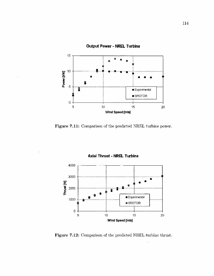
Output Power - NREL Turbine
15
10
o 0.
•
•
i • •
i -
• * • '
• Experimental
•SROTOR
10 15
Wind Speed [m/s]
20
Figure 7.11: Comparison of the predicted NREL turbine power.
Axial Thrust - NREL Turbine
4000
3000
H 2000
1000 II
m *_._* _
• * > •
n •
• Experimental
•SROTOR
10 15
Wind Speed [m/s]
20
Figure 7.12: Comparison of the predicted NREL turbine thrust.
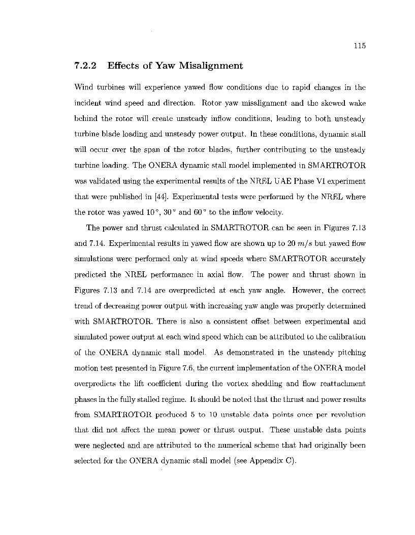
115
7.2.2 Effects of Yaw Misalignment
Wind turbines will experience yawed flow conditions due to rapid changes in the
incident wind speed and direction. Rotor yaw misalignment and the skewed wake
behind the rotor will create unsteady inflow conditions, leading to both unsteady
turbine blade loading and unsteady power output. In these conditions, dynamic stall
will occur over the span of the rotor blades, further contributing to the unsteady
turbine loading. The ONERA dynamic stall model implemented in SMARTROTOR
was validated using the experimental results of the NREL UAE Phase VI experiment
that were published in [44]. Experimental tests were performed by the NREL where
the rotor was yawed 10°, 30° and 60° to the inflow velocity.
The power and thrust calculated in SMARTROTOR can be seen in Figures 7.13
and 7.14. Experimental results in yawed flow are shown up to 20 m/s but yawed flow
simulations were performed only at wind speeds where SMARTROTOR accurately
predicted the NREL performance in axial flow. The power and thrust shown in
Figures 7.13 and 7.14 are overpredicted at each yaw angle. However, the correct
trend of decreasing power output with increasing yaw angle was properly determined
with SMARTROTOR. There is also a consistent offset between experimental and
simulated power output at each wind speed which can be attributed to the calibration
of the ONERA dynamic stall model. As demonstrated in the unsteady pitching
motion test presented in Figure 7.6, the current implementation of the ONERA model
overpredicts the lift coefficient during the vortex shedding and flow reattachment
phases in the fully stalled regime. It should be noted that the thrust and power results
from SMARTROTOR produced 5 to 10 unstable data points once per revolution
that did not affect the mean power or thrust output. These unstable data points
were neglected and are attributed to the numerical scheme that had originally been
selected for the ONERA dynamic stall model (see Appendix C).
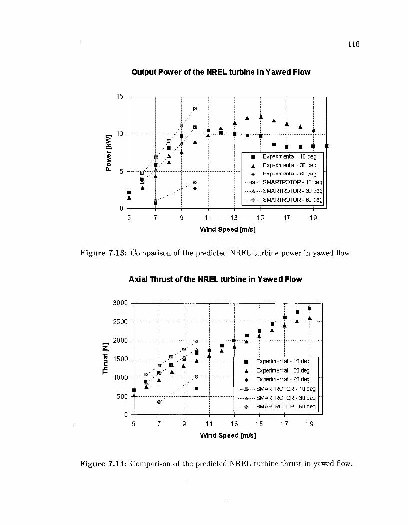
Output Power of the NREL turbine in Yawed Flow
15
10
o 5 4-
¥ A
*
• Experimental -10 deg A Experimental - 30 deg * Experimental - 60 deg
-a— SMARTROTOR-10 deg -4 —SMARTROTOR- 30 deg -©---SMARTROTOR- 60 deg
11 13 15
Wind Speed [m/s]
17 19
Figure 7.13: Comparison of the predicted NREL turbine power in yawed flow.
Axial Thrust of the NREL turbine in Yawed Flow
3000
2500
„ 2000 Z
| 1500
1000
500
0
• A
m ,M A
• A • A t
Experimental-10 deg
Experimental- 30 deg
Experimental- 60 deg
-SMARTROTOR-10deg
-SMARTROTOR-30 deg
SMARTROTOR - 60 deg
11 13
Wind Speed [m/s]
15 17 19
Figure 7.14: Comparison of the predicted NREL turbine thrust in yawed flow.
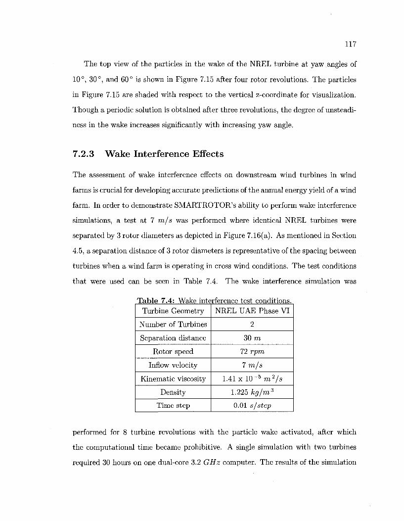
117
The top view of the particles in the wake of the NREL turbine at yaw angles of
10°, 30°, and 60° is shown in Figure 7.15 after four rotor revolutions. The particles
in Figure 7.15 are shaded with respect to the vertical z-coordinate for visualization.
Though a periodic solution is obtained after three revolutions, the degree of unsteadi
ness in the wake increases significantly with increasing yaw angle.
7.2.3 Wake Interference Effects
The assessment of wake interference effects on downstream wind turbines in wind
farms is crucial for developing accurate predictions of the annual energy yield of a wind
farm. In order to demonstrate SMARTROTOR's ability to perform wake interference
simulations, a test at 7 m/s was performed where identical NREL turbines were
separated by 3 rotor diameters as depicted in Figure 7.16(a). As mentioned in Section
4.5, a separation distance of 3 rotor diameters is representative of the spacing between
turbines when a wind farm is operating in cross wind conditions. The test conditions
that were used can be seen in Table 7.4. The wake interference simulation was
Table 7.4: Wake interference test conditions. Turbine Geometry
Number of Turbines
Separation distance
Rotor speed
Inflow velocity
Kinematic viscosity
Density
Time step
NREL UAE Phase VI
2
30 m
72 rpm
7 m/s
1.41 x 10~5 m2/s
1.225 kg/m3
0.01 s/step
performed for 8 turbine revolutions with the particle wake activated, after which
the computational time became prohibitive. A single simulation with two turbines
required 30 hours on one dual-core 3.2 GHz computer. The results of the simulation
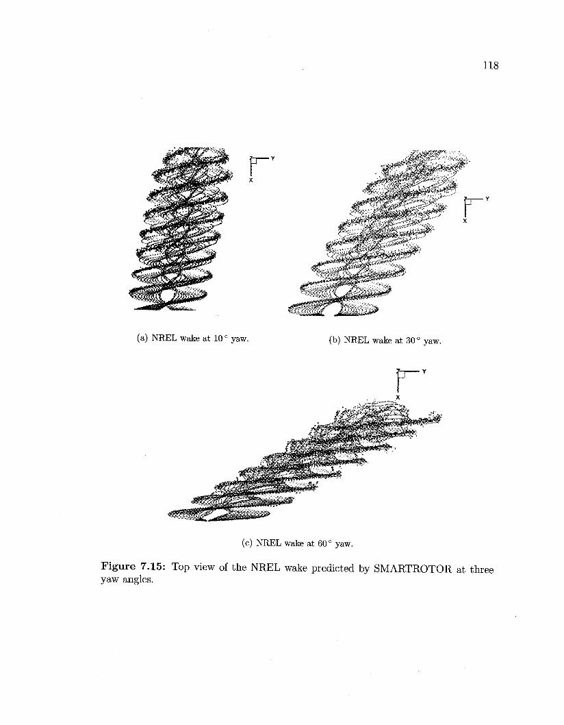
^5S*r3&*^
(a) NREL wake at 10 ° yaw. (b) NREL wake at 30° yaw.
(c) NREL wake at 60 ° yaw.
Figure 7.15: Top view of the NREL wake predicted by SMARTROTOR at three yaw angles.
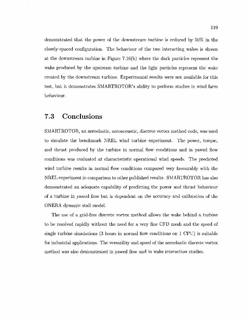
119
demonstrated that the power of the downstream turbine is reduced by 50% in the
closely-spaced configuration. The behaviour of the two interacting wakes is shown
at the downstream turbine in Figure 7.16(b) where the dark particles represent the
wake produced by the upstream turbine and the light particles represent the wake
created by the downstream turbine. Experimental results were not available for this
test, but it demonstrates SMARTROTOR's ability to perform studies in wind farm
behaviour.
7.3 Conclusions
SMARTROTOR, an aeroelastic, aeroacoustic, discrete vortex method code, was used
to simulate the benchmark NREL wind turbine experiment. The power, torque,
and thrust produced by the turbine in normal flow conditions and in yawed flow
conditions was evaluated at characteristic operational wind speeds. The predicted
wind turbine results in normal flow conditions compared very favourably with the
NREL experiment in comparison to other published results. SMARTROTOR has also
demonstrated an adequate capability of predicting the power and thrust behaviour
of a turbine in yawed flow but is dependent on the accuracy and calibration of the
ONERA dynamic stall model.
The use of a grid-free discrete vortex method allows the wake behind a turbine
to be resolved rapidly without the need for a very fine CFD mesh and the speed of
single turbine simulations (3 hours in normal flow conditions on 1 CPU) is suitable
for industrial applications. The versatility and speed of the aeroelastic discrete vortex
method was also demonstrated in yawed flow and in wake interaction studies.
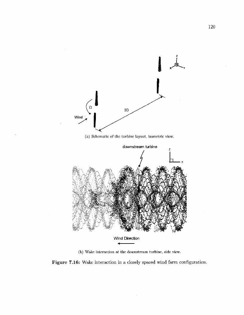
I
(a) Schematic of the turbine layout, isometric view,
downstream turbine
Wind Direction ^
(b) Wake interaction at the downstream turbine, side view.
Figure 7.16: Wake interaction in a closely spaced wind farm configuration.
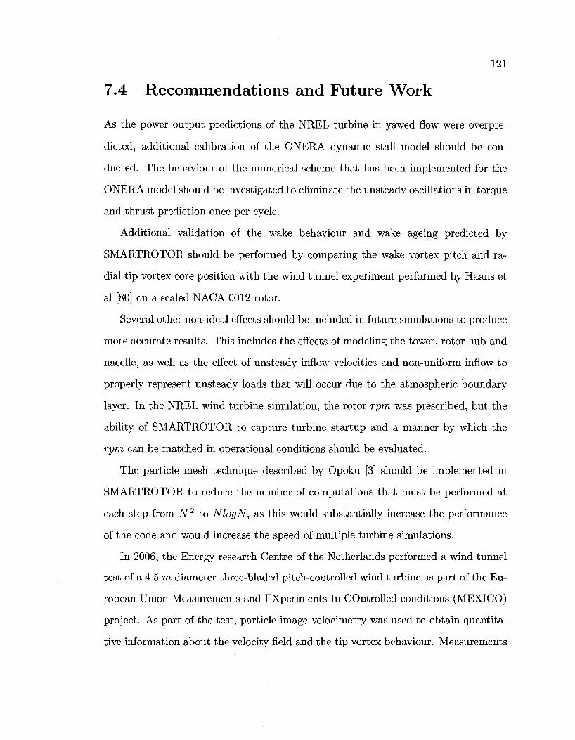
121
7.4 Recommendations and Future Work
As the power output predictions of the NREL turbine in yawed flow were overpre-
dicted, additional calibration of the ONERA dynamic stall model should be con
ducted. The behaviour of the numerical scheme that has been implemented for the
ONERA model should be investigated to eliminate the unsteady oscillations in torque
and thrust prediction once per cycle.
Additional validation of the wake behaviour and wake ageing predicted by
SMARTROTOR should be performed by comparing the wake vortex pitch and ra
dial tip vortex core position with the wind tunnel experiment performed by Haans et
al [80] on a scaled NACA 0012 rotor.
Several other non-ideal effects should be included in future simulations to produce
more accurate results. This includes the effects of modeling the tower, rotor hub and
nacelle, as well as the effect of unsteady inflow velocities and non-uniform inflow to
properly represent unsteady loads that will occur due to the atmospheric boundary
layer. In the NREL wind turbine simulation, the rotor rpm was prescribed, but the
ability of SMARTROTOR to capture turbine startup and a manner by which the
rpm can be matched in operational conditions should be evaluated.
The particle mesh technique described by Opoku [3] should be implemented in
SMARTROTOR to reduce the number of computations that must be performed at
each step from N2 to NlogN, as this would substantially increase the performance
of the code and would increase the speed of multiple turbine simulations.
In 2006, the Energy research Centre of the Netherlands performed a wind tunnel
test of a 4.5 m diameter three-bladed pitch-controlled wind turbine as part of the Eu
ropean Union Measurements and Experiments In Controlled conditions (MEXICO)
project. As part of the test, particle image velocimetry was used to obtain quantita
tive information about the velocity field and the tip vortex behaviour. Measurements
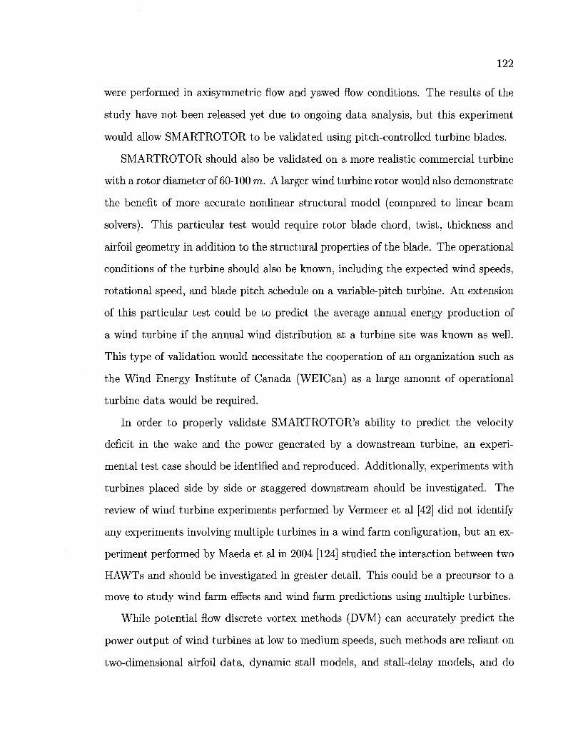
122
were performed in axisymmetric flow and yawed flow conditions. The results of the
study have not been released yet due to ongoing data analysis, but this experiment
would allow SMARTROTOR to be validated using pitch-controlled turbine blades.
SMARTROTOR should also be validated on a more realistic commercial turbine
with a rotor diameter of 60-100 m. A larger wind turbine rotor would also demonstrate
the benefit of more accurate nonlinear structural model (compared to linear beam
solvers). This particular test would require rotor blade chord, twist, thickness and
airfoil geometry in addition to the structural properties of the blade. The operational
conditions of the turbine should also be known, including the expected wind speeds,
rotational speed, and blade pitch schedule on a variable-pitch turbine. An extension
of this particular test could be to predict the average annual energy production of
a wind turbine if the annual wind distribution at a turbine site was known as well.
This type of validation would necessitate the cooperation of an organization such as
the Wind Energy Institute of Canada (WEICan) as a large amount of operational
turbine data would be required.
In order to properly validate SMARTROTOR's ability to predict the velocity
deficit in the wake and the power generated by a downstream turbine, an experi
mental test case should be identified and reproduced. Additionally, experiments with
turbines placed side by side or staggered downstream should be investigated. The
review of wind turbine experiments performed by Vermeer et al [42] did not identify
any experiments involving multiple turbines in a wind farm configuration, but an ex
periment performed by Maeda et al in 2004 [124] studied the interaction between two
HAWTs and should be investigated in greater detail. This could be a precursor to a
move to study wind farm effects and wind farm predictions using multiple turbines.
While potential flow discrete vortex methods (DVM) can accurately predict the
power output of wind turbines at low to medium speeds, such methods are reliant on
two-dimensional airfoil data, dynamic stall models, and stall-delay models, and do
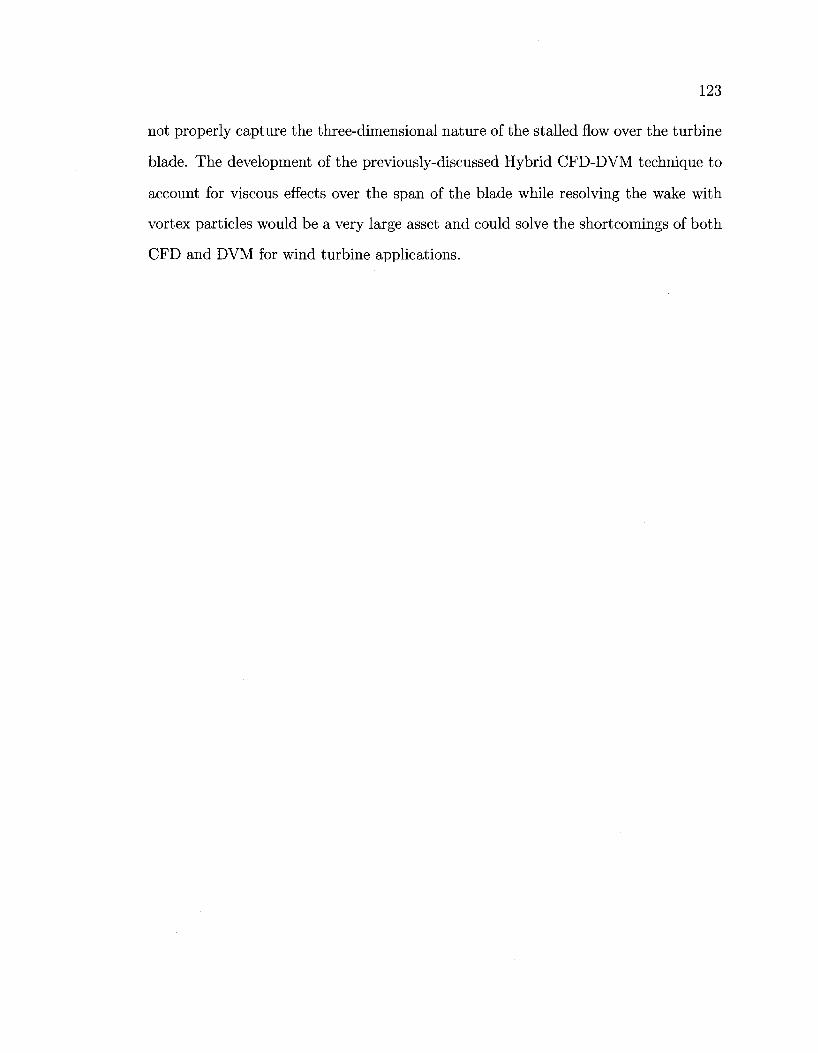
123
not properly capture the three-dimensional nature of the stalled flow over the turbine
blade. The development of the previously-discussed Hybrid CFD-DVM technique to
account for viscous effects over the span of the blade while resolving the wake with
vortex particles would be a very large asset and could solve the shortcomings of both
CFD and DVM for wind turbine applications.
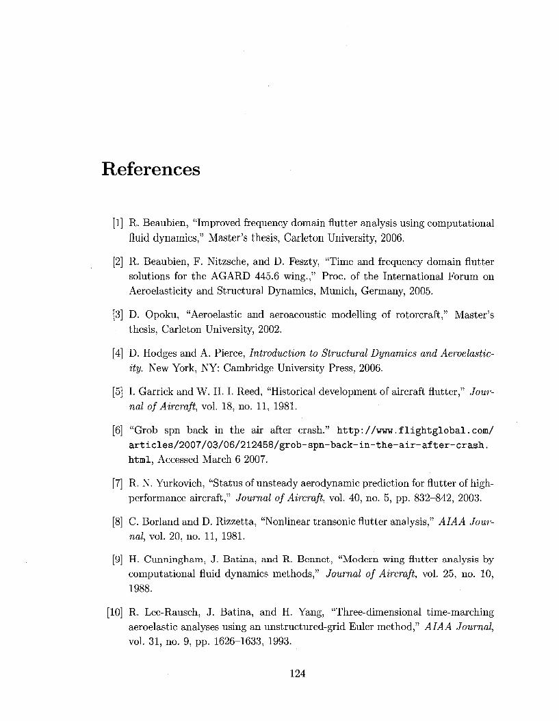
References
R. Beaubien, "Improved frequency domain flutter analysis using computational fluid dynamics," Master's thesis, Carleton University, 2006.
R. Beaubien, F. Nitzsche, and D. Feszty, "Time and frequency domain flutter solutions for the AGARD 445.6 wing.," Proc. of the International Forum on Aeroelasticity and Structural Dynamics, Munich, Germany, 2005.
D. Opoku, "Aeroelastic and aeroacoustic modelling of rotorcraft," Master's thesis, Carleton University, 2002.
D. Hodges and A. Pierce, Introduction to Structural Dynamics and Aeroelasticity. New York, NY: Cambridge University Press, 2006.
I. Garrick and W. H. I. Reed, "Historical development of aircraft flutter," Journal of Aircraft, vol. 18, no. 11, 1981.
"Grob spn back in the air after crash." http:/ /www.flightglobal.com/ ar t ic les /2007/03/06/212458/grob-spn-back- in- the-a i r -af ter -crash . html, Accessed March 6 2007.
R. N. Yurkovich, "Status of unsteady aerodynamic prediction for flutter of high-performance aircraft," Journal of Aircraft, vol. 40, no. 5, pp. 832-842, 2003.
C. Borland and D. Rizzetta, "Nonlinear transonic flutter analysis," AIAA Journal, vol. 20, no. 11, 1981.
H. Cunningham, J. Batina, and R. Bennet, "Modern wing flutter analysis by
computational fluid dynamics methods," Journal of Aircraft, vol. 25, no. 10, 1988.
R. Lee-Rausch, J. Batina, and H. Yang, "Three-dimensional time-marching aeroelastic analyses using an unstructured-grid Euler method," AIAA Journal, vol. 31, no. 9, pp. 1626-1633, 1993.
124

125
[11] E. Lee-Rausch and J. Batina, "Wing flutter boundary prediction using unsteady
Euler aerodynamic method," Journal of Aircraft, vol. 32, no. 2, 1995.
[12] G. S. L. Goura, Time Marching Analysis of Flutter Using Computational Fluid Dynamics. PhD thesis, University of Glasgow, 2001.
[13] C. Farhat, P. Geuzaine, and G. Brown, "Application of a three-field nonlinear fluid-structure formulation to the prediction of the aeroelastic parameters of an F-16 fighter," Computers and Fluids, vol. 32, pp. 3-29, 2003.
[14] K. J. Badcock, B. E. Richards, and M. A. Woodgate, "Elements of computational fluid dynamics on block structured grids using implicit solvers," Progress in Aerospace Sciences, vol. 36, pp. 351-392, 2000.
[15] G. Goura, K. Badcock, M. Woodgate, and B. Richards, "Implicit methods for the time marching analysis of flutter.," The Aeronautical Journal, vol. 105, pp. 169-215, 2001.
[16] "Modeling of turbulence in eros-uk," tech. rep., University of Glasgow, Scotland, 2002.
[17] M. Woodgate, K. Badcock, A. Rampurawala, and B. Richards, "Aeroelastic calculations for the hawk aircraft using the Euler equations," tech. rep., University of Glasgow, Scotland, 2003.
[18] E. Albano and W. Rodden, "A doublet-lattice method for calculating lift distributions on oscillating surfaces in subsonic flows," AIAA Journal, vol. 7, no. 2, pp. 279-285, 1969.
[19] R. G. A. da Silva, A study on correction methods for aeroelastic analysis in transonic flow. PhD thesis, Sao Jose dos Campos, 2004.
[20] R. Bisplinghoff, H. Ashley, and R. Halfman, Aeroelasticity. Mineola, NY: Dover Publications, Inc., 1983.
[21] J. Giesing, T. Kalman, and W. Rodden, "Subsonic unsteady aerodynamics for general configurations, direct application of the non-planar doublet-lattice method," tech. rep., Wright-Patterson Air Force Base, 1972.
[22] T. Kalman, W. Rodden, and J. Giesing, "Aerodynamic influence coefficients by the doublet lattice method for interfering non planar lifting surfaces oscillating in a subsonic flow," tech. rep., 1969.

126
[23] J. D. J. Anderson, Fundamentals of Aerodynamics. New York: McGraw Hill, 3 ed., 2001.
[24] O. Mello, An improved hybrid Navier-Stokes/Full-Potential Method for Computation of Unsteady Compressible Flows. PhD thesis, Georgia Institute of Technology, 1994.
[25] E. Yates, N. Land, and J. Foughner, "Measured and calculated subsonic and transonic flutter characteristics of a 45 ° sweptback wing planform in air and in freon-12 in the Langley transonic dynamics tunnel.," tech. rep., Langley Research Center, Virginia, 1963.
[26] H. Tijdeman and J. W. G. van Nunen, "Transonic wind-tunnel tests on an oscillating wing with external store, part 1: General description," NLR TR 78105 U Part 1, 1978.
[27] R. M. Kolonay, Unsteady Aeroelastic Optimization in the Transonic Regime. PhD thesis, Purdue University, 1996.
[28] W. P. Rodden and J. D. Revell, "The status of unsteady aerodynamic influence coefficients," Fairchild Fund Paper FF-33, 1962.
[29] K. Gupta, "Development of a finite element aeroelastic analysis capability.," Journal of Aircraft, vol. 33, no. 5, 1996.
[30] C. Liu, Y. Zhu, and et al, "Calculation of wing flutter by a coupled fluid-structure method," Journal of Aircraft, vol. 38, no. 2, 2001.
[31] C. Farhat and M. Lesoinne, "High order staggered and subiteration-free algorithm for nonlinear transient aeroelastic problems," AIAA Journal, vol. 36, no. 9, pp. 1754-1757, 1998.
[32] K. J. Badcock, M. A. Woodgate, and B. Richards, "Direct aeroelastic bifurcation analysis of a symmetric wing based on the Euler equations.," tech. rep., University of Glasgow, Scotland, 2003.
[33] "World wind energy - press release." World Wind Energy Association, February 2008.
[34] E. Hau, Wind Turbines: Fundamentals, Technologies, Application and Eco
nomics. Springer, 2 ed., 2005.
127
[35] D. A. Spera, ed., Wind Turbine Technology: Fundamental Concepts of Wind Turbine Engineering. New York: ASME Press, 1994.
[36] S. Gupta, Development of a time-accurate viscous Lagrangian vortex wake model for wind turbine applications. PhD thesis, University of Maryland, 2006.
[37] M. S. Chappel, "Wind energy research and development at the national research council Canada, 1975-1985," tech. rep., National Research Council Canada, Ottawa, Ontario, Canada, 1986.
[38] S. Guha, H. Soloumah, and N. Kar, "Status of and prospect for wind power generation in Canada," Wind Engineering, vol. 29, no. 3, pp. 253-270, 2005.
[39] "Wind farms." h t t p : //www. canwea. ca/f arms/index_e. php, Accessed May 25 2008.
[40] "Basic principles of wind resource evaluation." http://www.awea.org/faq/ basicwr.html, Accessed May 15 2008.
[41] J. G. Leishman, "Challenges in modeling the unsteady aerodynamics of wind turbines," Wind Energy, vol. 5, 2002.
[42] J. Vermeer, L., J. Sorensen, and A. Crespo, "Wind turbine wake aerodynamics," Progress in Aerospace Sciences, vol. 39, 2003.
[43] S. Schreck, "The NREL full-scale wind tunnel experiment - introduction to the special issue," Wind Energy, vol. 5, 2002.
[44] S. Gupta and J. Leishman, "Performance predictions of the NREL phase VI combined experiment rotor using a free-vortex wake model," Proc. of the 44th AIAA Aerospace Sciences Meeting and Exhibit, Paper AIAA 2006-390, Reno, Nevada, 2006.
[45] J. G. Leishman, Principles of Helicopter Aerodynamics. Cambridge Aerospace Series, New York: Cambridge University Press, 2 ed., 2006.
[46] "GH WindFarmer validation report," tech. rep., Bristol, England, 2003.
[47] H. M., J. Sorensen, S. Voutsinas, and et al., "State of the art in wind turbine aerodynamics and aeroelasticity," Progress in Aerospace Sciences, vol. 42, 2006.
128
[48] D. Simms, S. Schreck, M. Hand, and L. Fingersh, "NREL Unsteady Aerodynamics Experiment in the NASA-Ames wind tunnel: A comparison of predictions to measurements," NREL/TP-500-29494, National Renewable Energy Laboratory, Golden, Colorado, USA, 2001.
[49] I. Katie, J. Hostrup, and N. Jensen, "A simple model for cluster efficiency," Proc. of the European Wind Energy Conference, 1986.
[50] "GH WindFarmer theory manual," tech. rep., Bristol, England, 2007.
[51] J. F. Ainslie, "Calculating the flowfield in the wake of wind turbines," Journal
of Wind Engineering and Industrial Aerodynamics, vol. 27, 1988.
[52] B. Lange and et al, "Modeling of offshore wind turbine wakes with the wind farm program FLaP," Proc. of the OWEMES conference, 2003.
[53] J. Ainslie, U. Hassan, and et al, "A wind tunnel investigation of the wake structure within small wind turbine farms," Proc. of the European Wind Energy Conference, P. 547-551, Glasgow, Scotland, 1989.
[54] "Clean energy project analysis: Retscreen engineering and cases." h t t p : //www. retscreen.net /ang/12.php, Updated Nov 2 2007. Accessed May 2 2008.
[55] "Wasp wake model." http://www.wasp.dk/Products/WAsP/ WakeEffectModel.html, Updated Aug 2007. Accessed May 7 2008.
[56] "WAsP 9 help facility and on-line documentation." http://www.wasp.dk/ Support/FAQ/WebHelp/Wasp9.htm, Updated 2007. Accessed May 7 2008.
[57] A. Bowen and N. Mortensen, "Exploring the limits of WAsP the wind atlas analysis and application program," Proc. of the European Union Wind Energy Conference, Sweden, May 1996.
[58] "Oldenburg university wind farm layout program FLaP." http://www. forwind.de/gb/produkte_dienstleistungen/flap/index.shtml, Accessed May 7 2008.
[59] G. Schepers, "Modelling of wake aerodynamics -1- new farm control strategies," Dutch Wind Workshops, Presentation Slides, October 2006.
[60] W. Schlez and et al., "ENDOW: Improvement of wake models within offshore wind farms," Wind Engineering, vol. 25, no. 5, 2001.
129
[61] H. Glauert, "Airplane propellers," in Aerodynamic Theory (W. P. Durand, ed.), vol. 4, (Berlin, Germany), pp. 169-360, Springer-Verlag, 1935.
[62] S. Gupta and J. Leishman, "Comparison of momentum and vortex methods for the aerodynamic analysis of wind turbines,"
[63] M. Hansen, Aerodynamics of Wind Turbines. New York: Earthscan Publications Ltd., 1 ed., 2001.
[64] T. Burton, D. Sharpe, N. Jenkins, and E. Bossanyi, Wind Energy Handbook. New York: John Wiley and Sons, 2001.
[65] D. Molenaar and S. Dijkstra, "State-of-the-art of wind turbine design codes: Main features overview for cost-effective generation," Wind Engineering, vol. 23, 1999.
[66] C. Masson, I. Ammara, and I. Paraschivoiu, "An aerodynamic method for the analysis of isolated horizontal-axis wind turbines," International Journal of Rotating Machines, vol. 3, pp. 21-32, 1997.
[67] T. Wu, "Flow through a heavily loaded actuator disk," Schiffstechnik, vol. 9, pp. 134-138, 1962.
[68] C. Masson, I. Ammara, C. Leclerc, and I. Paraschivoiu, "Numerical simulations of the three-dimensional turbulent flow in a wind park," AIAA Journal - AIAA 98-0058, 1998.
[69] I. Ammara, C. Leclerc, and C. Masson, "A viscous three-dimensional differential/actuator-disk method for aerodynamic analysis of wind farms," Journal of Solar Energy - T ASME, vol. 124, no. 4, pp. 345-356, 2002.
[70] N. Sorensen, J. and C. Kock, "A model for unsteady rotor aerodynamics," Journal of Wind Engineering and Industrial Aerodynamics, vol. 39, pp. 139-149, 1992.
[71] J. Robison, D., F. Coton, R. Galbraith, and M. Vezza, "Application of a prescribed wake aerodynamic prediction scheme to horizontal axis wind turbines in axial flow," Wind Engineering, vol. 19, no. 1, pp. 41-51, 1995.
[72] S. Lain, J. Garcia, and R. Aliod, "Development of a lifting surface - 2D panel method to compute the three-dimensional pressure distribution over the blade of a horizonta-axis wind turbine," Wind Engineering, vol. 19, 1995.
130
[73] T. Wang and F. Coton, "An unsteady aerodynamic model for HAWT performance including tower shadow effects," Wind Engineering, vol. 23, 1999.
[74] S. Schmitz and J.-J. Chattot, "Method for aerodynamic analysis of wind turbines at peak power," AIAA Journal of Propulsion and Power - Technical Notes, vol. 23, no. 1, 2007.
[75] R. Bareiss and S. Wagner, "The free wake/hybrid wake code ROVLM - a tool for the aerodynamic analysis of wind turbines," Proc. of the European Community Wind Energy Conference, P. 424-427, Germany, 1993.
[76] J. Whale, C. G. Anderson, R. Bareiss, and S. Wagner, "An experimental and numerical study of the vortex structure in the wake of a wind turbine," Journal of Wind Engineering and INdustrial Aerodynamics, vol. 84, 2000.
[77] E. Duque, M. Burklund, and W. Johnson, "Navier-Stokes and comprehensive analysis performance predictions of the NREL Phase VI experiment," Proc. of the 41st AIAA Aerospace Sciences Meeting and Exhibit, Paper AIAA 2003-355, Reno, Nevada, 2003.
[78] S. Gupta and J. Leishman, "Validation of a free-vortex wake model for wind turbines in yawed flow," Proc. of the 44th AIAA Aerospace Sciences Meeting and Exhibit, Paper AIAA 2006-389, Reno, Nevada, 2006.
[79] S. Gupta and J. Leishman, "Dynamic stall modeling of the S809 airfoil and comparison with experiments," Proc. of the 44th AIAA Aerospace Sciences Meeting and Exhibit, Paper AIAA 2006-196, Reno, Nevada, 2006.
[80] W. Haans, T. Sant, G. Kuik, and G. Bussel, "Measurement and modelling of tip vortex paths in the wake of a HAWT under yawed flow conditions," Proc. of the 43rd AIAA Aerospace Sciences Meeting and Exhibit, Paper AIAA 2005-590, Reno, Nevada, 2005.
[81] A. Afjeh and T. Keith, "A simplified free wake method for horizontal-axis wind turbine performance prediction," Transactions of the ASME Journal of Fluids Engineering, vol. 108, pp. 303-309, 1986.
[82] F. Simoes and J. Graham, "Preidiction of loading on a horizontal axis wind turbine using a free vortex wake model," Proc. of the GWEA Conference, 1991.
[83] S. Voutsinas, M. Belessis, and S. Huberson, "Dynamic inflow effects and vortex particle methods," Proc. of the European Community Wind Energy Conference, P. 428-431, Germany, 1993.
131
[84] D. Opoku, D. Triantos, F. Nitzsche, and S. Voutsinas, "Rotorcraft aerodynamic and aeroacoustic modelling using vortex particle methods," Proc. of the ICAS 2002 Congress, The International Council of the Aeronautical Sciences, Toronto, Canada, 2002.
[85] D. G. Opoku and F. Nitzsche, "Acoustic validation of a new code using particle wake aerodynamics and geometrically-exact beam structural dynamics," Proc. of the 29th European Rotorcraft Forum, Germany, 2003.
[86] C. Cesnik, D. Opoku, F. Nitzsche, and T. Cheng, "Active twist rotor blade modelling using particle-wake aerodynamics and geometrically exact beam structural dynamics," Journal of Fluids and Structures, vol. 19, pp. 651-668, 2004.
[87] N. N. Sorensen, J. Michelsen, and S. Schreck, "Navier-Stokes predictions of the NREL Phase VI rotor in the NASA Ames 80 ft x 120 ft wind tunnel," Wind Energy, vol. 5, 2002.
[88] N. Sezer-Uzol and L. Long, "3-D time-accurate CFD simulations of wind turbine rotor flow fields," Proc. of the 44th AIAA Aerospace Sciences Meeting and Exhibit, Paper AIAA 2006-394, Reno, Nevada, 2003.
[89] F. Massouh, T. Dobrev, and M. Rapin, "Experimental and numerical survey in the wake of a wind turbine," Proc. of the 45th AIAA Aerospace Sciences Meeting and Exhibit, Paper AIAA 2007-423, Reno, Nevada, 2007.
[90] S. Benjanirat and L. Sankar, "Evaluation of turbulence models for the prediction of wind turbine aerodynamics," Proc. of the 41st AIAA Aerospace Sciences Meeting and Exhibit, Paper AIAA 2003-0517, Reno, Nevada, 2003.
[91] C. Tongchitpakdee, S. Benjanirat, and L. Sankar, "Nmerical simulation of the aerodynamics of horizontal axis wind turbines under yawed flow conditions," Proc. of the 43rd AIAA Aerospace Sciences Meeting and Exhibit, Paper AIAA 2005-773, Reno, Nevada, 2005.
[92] G. Xu, Computational Studies of Horizontal Wind Turibnes. PhD thesis, Georgia Institute of Technology, 2001.
[93] S. Benjanirat and L. Sankar, "Recent improvements to a combined navier-stokes full potential methodology for modeling horizontal axis wind turbines," 42nd AIAA Aerospace Sciences Meeting and Exhibit, Paper AIAA 2004-830, Reno, Nevada, 2004.
132
[94] P. Chaviaropoulos, "Development of a state-of-the-art aeroelastic simulator for horizontal axis wind turbines part 1: Structural aspects," Wind Engineering, vol. 20, no. 6, pp. 405-421, 1996.
[95] A. Hansen and D. Laino, "Validation study for AeroDyn and YawDyn using phase III combined experiment data (prediction of turbine dynamics)," Proc. of the 35th AIAA Aerospace Sciences Meeting and Exhibit, Paper 97-0943, Reno, Nevada, 1997.
[96] D. Hodges, "Review of composite rotor blade modeling," AIAA Journal - Technical Notes, vol. 28, no. 3, pp. 561-565, 1999.
[97] M. Hand, D. Simms, L. Fingersh, and et al., "Unsteady Aerodynamics Experiment Phase VI: Wind tunnel test configuration and available data campaigns," NREL/TP-500-29955, National Renewable Energy Laboratory, Golden, Colorado, USA, 2001.
[98] S. Voutsinas, M. Belessis, and K. Rados, "Investigation of the yawed operation of wind turbines by means of a vortex particle method," tech. rep.
[99] S. Voutsinas and D. Triantos, "High-resolution aerodynamic analysis of full helicopter configurations," Proc. of the 25th European Rotorcraft Forum, Rome, Italy, 1999.
[100] S. Voutsinas, "A generalized unsteady vortex particle method for solving the unsteady flow around multi-component configurations," tech. rep., National Technical University of Athens, Athens, Greece, 1990.
[101] J. Marshall, Inviscid Incompressible Flow. Wiley, 2001.
[102] J. Hess and A. Smith, "Calculation of potential flow about arbitrary bodies," Progress in Aeronautical Sciences, vol. 8.
[103] C. Rehbach, "Calcul d'ecoulements autour d'ailes sans epaisseur avec nappes tourbillonnaires evolutives," la Recherche Aerospatiale, no. 2, pp. 53-61, 1973.
[104] J. Beale and A. Majda, "Vortex methods I: Convegence in three dimensions," Mathematics of Computation, vol. 39, no. 159, pp. 1-27, 1982.
[105] J. Beale and A. Majda, "High order accurate vortex methods with explicit velocity kernels," Journal of Computational Physics, vol. 58, pp. 188-208, 1985.
133
[106] J. Larsen, S. Nielsen, and S. Krenk, "Dynamic stall model for wind turbine airfoils," Journal of Fluids and Structures, vol. 23, pp. 959-982, 2007.
[107] C. T. Tran and D. Petot, "Semi-empirical model for the dynamic stall of airfoils in view to the application to the calculation of responses of a helicopter blade in forward flight," Vertica, vol. 5, no. 1, pp. 35-53, 1981.
[108] D. Gross and F. Harris, "Prediction of in-flight stalled airloads from oscillating airfoil data," Proc. of the 25th annual forum of the American Helicopter Society, Washington DC, 1969.
[109] J. Leishman and T. Beddoes, "A semi-empirical model for dynamic stall," Journal of the American Helicopter Society, vol. 34, no. 3, pp. 3-17, 1989.
[110] S. Voutsinas, V. Riziotis, and P. Chaviaropoulos, "Non-linear aerodynamics and fatigue loading on wind turbines operating at extreme sites," Proc. of the 35th AIAA Aerospace Sciences Meeting and Exhibit, Paper AIAA 97-0935, Reno, Nevada, 1997.
[Ill] D. Petot, "Differential equation modeling of dynamic stall," La Recherche Aerospatiale, vol. 5, pp. 59-72, 1989.
[112] D. Peters, "Toward a unified lift model for use in rotor blade stability analysis," Journal of the American Helicopter Society, vol. 30, pp. 32-42, 1985.
[113] W. Bierbooms, "A comparison between unsteady aerodynamic models," Journal of Wind Engineering and Industrial Aerodynamics, vol. 39, pp. 23-33, 1992.
[114] D. Tang and E. Dowell, "Comments on the ONERA stall aerodynamic model and its impact on aeroelastic stability," Journal of Fluids and Structures, vol. 10, pp. 353-366, 1996.
[115] K. McAlister, O. Lambert, and D. Petot, "Application of the ONERA model of dynamic stall," NASA technical paper 2399, National Aeronautics and Space Administration, 1984.
[116] D. Hodges, "A mixed variational formulation based on exact intrinsic equations for dynamics of moving beams," International Journal of Solids and Structures, vol. 26, no. 11, pp. 1253-1273, 1990.
[117] X. Shang, Aeroelastic Stability of Composite Hingeless Rotors with Finite-State Unsteady Aerodynamics. PhD thesis, Georgia Institute of Technology, 1995.
134
[118] T. Cheng, "Structural dynamics modelling of helicopter blades for computational aeroelasticity," Master's thesis, Massachusetts Institute of Technology, 2002.
[119] S. Shin, Integral Twist Actuation of Helicopter Rotor Blades for Vibration Reduction. PhD thesis, Massachusetts Institute of Technology, 2001.
[120] W. H. Press, Numerical Recipes in FORTRAN 77: The Art of Scientific Computing. New York: Cambridge University Press, 1992.
[121] D. Somers, "Design and experimental results for the s809 airfoil," NREL/SR-440-6918, National Renewable Energy Laboratory, Golden, Colorado, USA, 1997.
[122] R. Ramsay, M. Hoffman, and G. Gregorek, "Effects of grit roughness and pitch oscillations on the s809 airfoil," NREL/TP-442-7817, National Renewable Energy Laboratory, Golden, Colorado, USA, 1995.
[123] V. Riziotis, S. Voutsinas, and A. Zervos, "Investigation of the yaw induced stall and its impact to the design of wind turbines," tech. rep., National Technical University of Athens, Athens, Greece.
[124] T. Maeda, T. Yokota, Y. Shimizu, and K. Adachi, "Wind tunnel study of the interaction between two horizontal axis wind turbines," Wind Engineering, vol. 28, no. 2, pp. 197-209, 2004.
Appendix A
Derivation of the AlC-correction Fourier
Transform
In order to transform the nonlinear lifting pressures obtained from rigid body os
cillatory pitch CFD simulations into the frequency domain, the unsteady pressures
must be Fourier transformed, following which they can be used to correct the linear
frequency domain solution to account for nonlinear transonic effects. The following
derivation has been reproduced from the work of Mello [24] for completeness and was
used by Silva [19] in a similar AlC-correction procedure.
The unsteady oscillatory pitch simulations were performed about a mean angle of
0 °. The complex representation of the motion of the wing during the CFD simulations
is given by Equation A.l
oF (r) = AaeikT (A.l)
where r is the non-dimensional time step, k is the reduced frequency of the pitching
motion, a is the angle of attack, and the superscript c is the complex representation
of the angle of attack at a particular time step. The complex representation of the
steady-state response is given by Equation A.2.
CCP (r) = [Re (CPi) + Urn {CPi)} eikT (A.2)
135
136
The actual motion of the wing is described by the imaginary part of Equation A.l
and so the actual response is described by the imaginary part of Equation A.2. The
actual response CP(T) can be related to the complex representation by Equation A.3
C£ (r) = [Re (CPi) + ilm (CPi)] eikT
= [Re (Cpi) cos (kr) — Im (Cp*) sin (kr)] + i [Re (Cpi) sin (kr) + Im {CPi) cos (kr)]
(A.3)
The imaginary portion of Equation A.3 corresponds to the pressure coefficient re
sponse, as described by Equation A. 4.
CP (r) = [Re {CPi) sin (kr) + Im (CPi) cos (kr)] (A.4)
The real and imaginary components of the unsteady pressure at a particular spanwise
location i can be obtained in terms of the actual pressure coefficient response described
by Equations A.5 and A.6.
T-I+2-K/U
Re (CPi) = - f CP (r) sin {kr) dr (A.5)
Tl
Ti+2ir/fc
Im(CPi) = - f CP (r) cos (kr) dr (A.6)
Tl
In Equations A.5 and A.6, T\ should be selected so that the transient portion of the
unsteady response is not included in the Fourier transform. The real and imaginary
components of the lifting pressures are determined from the discrete Fourier transform
137
of the above two Equations, as seen in Equations A.7 and A.8
kAr mi^T
Re(CPi) = — — 2 ^ CPmsm{kmAr) (A.7) 2nAa
m=rni
kAr mi+mT
Im(Cpi) = ^ j ^ Yl CPmcos(kmAr) (A.8) ra=mi
where m refers to the time step number, mi = T\/AT and rrix = 2n/kAr. The above
two Equations have been normalized with respect to the amplitude of oscillation 2 Aa
and it should be noted that the discrete Fourier transform used in this work as well
as that of Silva [19] includes the Mach number (M) in the numerator as well.
Appendix B
Geometric and Structural Properties of
the NREL UAE Phase VI Wind Turbine
The model of the NREL turbine blade was created based on the geometric and struc
tural information provided by the NREL in [97]. The experimental NREL blade
begins at a radius r = 0.508 m from the centre of the hub with a cylindrical section
until r = 0.883 m. The blade then transitions from a cylindrical cross-section to the
S809 airfoil at r = 1.257 m. In order to simplify the blade for SMARTROTOR, the
cylindrical and transitional sections were neglected and the root of the blade model
was initiated at r = 1.008 m with the S809 airfoil.
The chord and twist distributions of the NREL blade were interpolated to the 17
spanwise panel nodes, as seen in Table B.l, but the blade thickness to chord ratio
of 21% was neglected due to the thin wing representation of the airfoil. The twist
distribution described in Table B.l is positive towards the feathered blade position,
and the tip pitch angle was set to 3 ° for the simulations.
The structural properties of the NREL blade were provided in [97] and were
interpolated to the centre of each of the 16 elements of the structural model. The
mass and stiffness data required at each radial strip in SMARTROTOR includes the
principal mass moments of inertia, the directional mass distribution on each element,
138
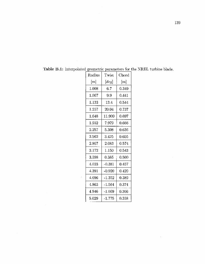
Table B.l: Interpolated geometric parameters for the NREL turbine blade.
Radius
[m]
1.008
1.067
1.133
1.257
1.648
1.952
2.257
2.562
2.867
3.172
3.598
4.023
4.391
4.696
4.863
4.946
5.029
Twist
[deg]
6.7
9.9
13.4
20.04
11.909
7.979
5.308
3.425
2.083
1.150
0.385
-0.381
-0.920
-1.352
-1.564
-1.669
-1.775
Chord
[m]
0.349
0.441
0.544
0.737
0.697
0.666
0.636
0.605
0.574
0.543
0.500
0.457
0.420
0.389
0.374
0.366
0.358
140
the axial stiffness, the torsional stiffness, the flapwise and lead-lag stiffness, and the
elastic axis of the wing. The structural properties used to model the NREL blade
span can be seen Table B.2.
The third component to the NREL blade model was two-dimensional airfoil data
for the S809 airfoil that was used for viscous corrections to the potential forces deter
mined with SMARTROTOR. The NREL report [97] included two-dimensional airfoil
data obtained from an experiment performed at the Ohio State University [122]. The
two-dimensional wind tunnel test performed on the S809 in Reference [122] contained
data at Reynolds numbers from 0.75 to 1.5 million. The lift, drag, and moment co
efficients were available from a — —20° to a = +26° at Reynolds numbers of 0.75
x 106, 1.0 x 10⁶, and 1.5 x 10⁶. However, at a Reynolds number of 1.25 x 10⁶,
two-dimensional coefficients were available up to +40°. As the S809 airfoil did not
exhibit high sensitivity to the Reynolds number in [122], the coefficients at high angle
of attack (above 26°) at a Reynolds number of 1.25 x 10 6 were used to extend the
data sets at the other three Reynolds numbers.
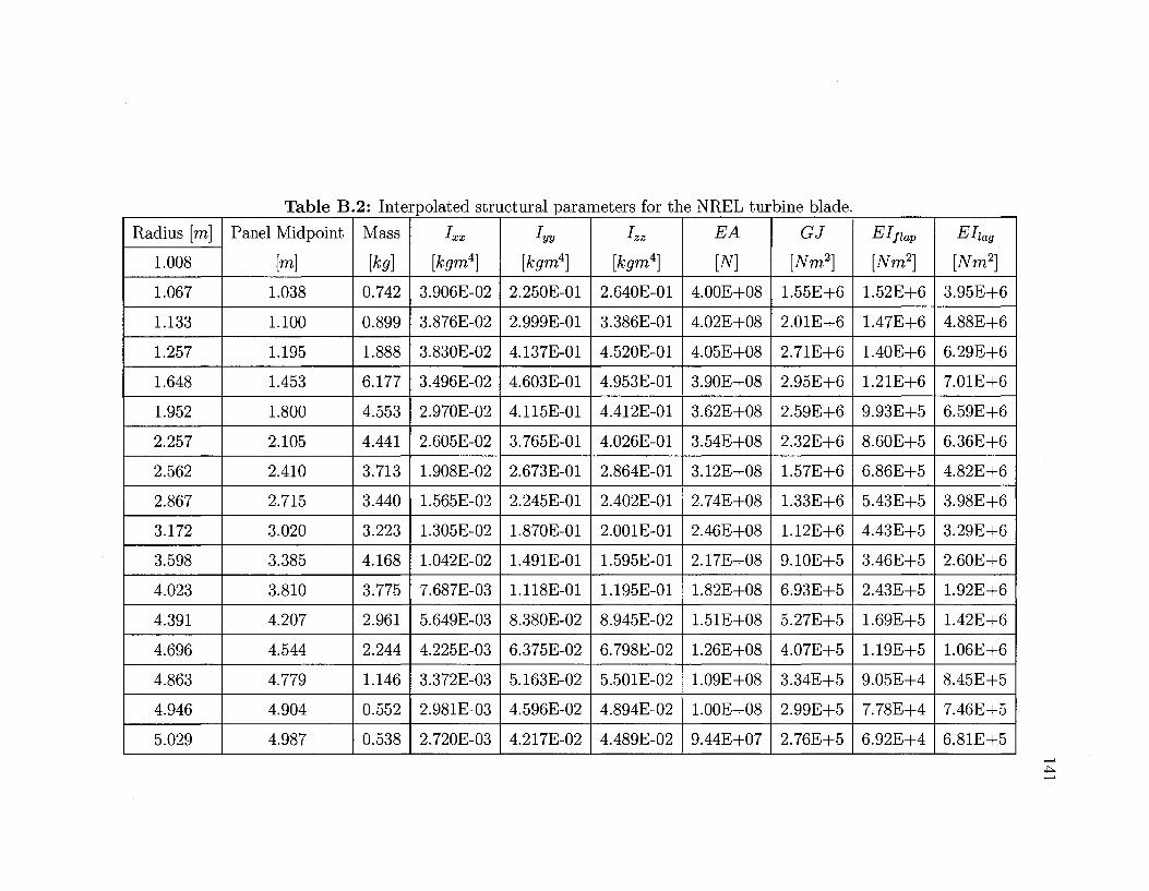
Table B.2: Interpolated structural parameters for the NREL turbine blade.
Radius [m]
1.008
1.067
1.133
1.257
1.648
1.952
2.257
2.562
2.867
3.172
3.598
4.023
4.391
4.696
4.863
4.946
5.029
Panel Midpoint
[m]
1.038
1.100
1.195
1.453
1.800
2.105
2.410
2.715
3.020
3.385
3.810
4.207
4.544
4.779
4.904
4.987
Mass
0.742
0.899
1.888
6.177
4.553
4.441
3.713
3.440
3.223
4.168
3.775
2.961
2.244
1.146
0.552
0.538
[kgm4]
3.906E-02
3.876E-02
3.830E-02
3.496E-02
2.970E-02
2.605E-02
1.908E-02
1.565E-02
1.305E-02
1.042E-02
7.687E-03
5.649E-03
4.225E-03
3.372E-03
2.981E-03
2.720E-03
[kgm4]
2.250E-01
2.999E-01
4.137E-01
4.603E-01
4.115E-01
3.765E-01
2.673E-01
2.245E-01
1.870E-01
1.491E-01
1.118E-01
8.380E-02
6.375E-02
5.163E-02
4.596E-02
4.217E-02
•Izz
[kgm4]
2.640E-01
3.386E-01
4.520E-01
4.953E-01
4.412E-01
4.026E-01
2.864E-01
2.402E-01
2.001E-01
1.595E-01
1.195E-01
8.945E-02
6.798E-02
5.501E-02
4.894E-02
4.489E-02
EA
[N]
4.00E+08
4.02E+08
4.05E+08
3.90E+08
3.62E+08
3.54E+08
3.12E+08
2.74E+08
2.46E+08
2.17E+08
1.82E+08
1.51E+08
1.26E+08
1.09E+08
1.00E+08
9.44E+07
GJ
[Nm2]
1.55E+6
2.01E+6
2.71E+6
2.95E+6
2.59E+6
2.32E+6
1.57E+6
1.33E+6
1.12E+6
9.10E+5
6.93E+5
5.27E+5
4.07E+5
3.34E+5
2.99E+5
2.76E+5
EI flap
[Nm2]
1.52E+6
1.47E+6
1.40E+6
1.21E+6
9.93E+5
8.60E+5
6.86E+5
5.43E+5
4.43E+5
3.46E+5
2.43E+5
1.69E+5
1.19E+5
9.05E+4
7.78E+4
6.92E+4
Ellag
[Nm2]
3.95E+6
4.88E+6
6.29E+6
7.01E+6
6.59E+6
6.36E+6
4.82E+6
3.98E+6
3.29E+6
2.60E+6
1.92E+6
1.42E+6
1.06E+6
8.45E+5
7.46E+5
6.81E+5
Appendix C
Implementation of the ONERA dynamic
stall model
The original ONERA dynamic stall model was implemented in GENUVP and modi
fied in SMARTROTOR for the S809 airfoil. The dynamic stall model was developed
for pitching motions though it can be used for more general motions. An aerody
namic coefficient C is expressed as the sum of two terms in the ONERA dynamic
stall model; one term C\ to account for the attached component of the flow and a
second term Ci to account for the separated flow, as seen in Equation C.l.
0 = ^ + 02 (C.l)
The lift, drag, and pitching moment models will be presented below with the
corresponding discretization, following which the coefficients used in the current work
will be shown. The subscripts z, x, and m in the following sections refer to the lift,
drag, and pitching moment coefficients, respectively, for consistency with the original
ONERA report [111]. In the original report however, the angle of attack is written
as © whereas a will be used here.
142
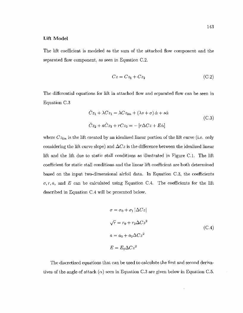
143
Lift Model
The lift coefficient is modeled as the sum of the attached flow component and the
separated flow component, as seen in Equation C.2.
Cz = Cz1 + Cz2 (C.2)
The differential equations for lift in attached flow and separated flow can be seen in
Equation C.3
Cz\ + XCzi — XCzun + (As + a) a + sa (C.3)
Cz2 + aCz2 + rCz2 = - [rACz + Ea]
where Czun is the lift created by an idealized linear portion of the lift curve (i.e. only-
considering the lift curve slope) and ACz is the difference between the idealized linear
lift and the lift due to static stall conditions as illustrated in Figure C.l. The lift
coefficient for static stall conditions and the linear lift coefficient are both determined
based on the input two-dimensional airfoil data. In Equation C.3, the coefficients
cr,r,a, and E can be calculated using Equation C.4. The coefficients for the lift
described in Equation C.4 will be presented below.
a — <j0 + o\ \ACz\
Vr = r0 + r2ACz2
(C.4)
a = a0 + a2ACz2
E = E2ACz2
The discretized equations that can be used to calculate the first and second deriva
tives of the angle of attack (a) seen in Equation C.3 are given below in Equation C.5.
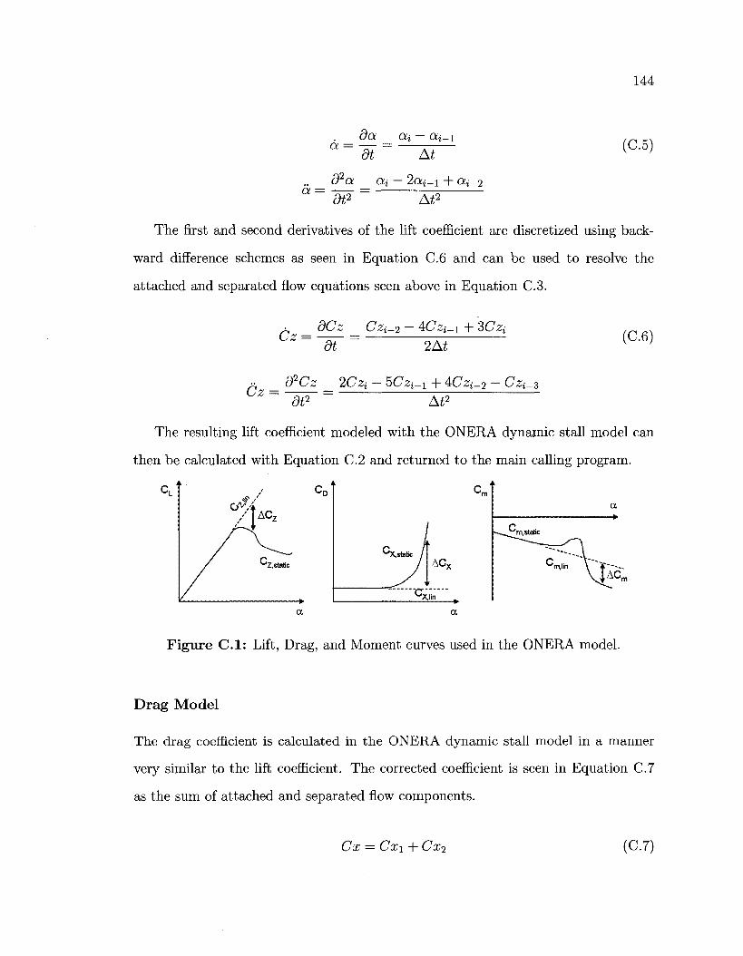
144
a =
da oii — oii-i a = ~dt= A*
d2a ai — 2ctj_i + a
(C.5)
i - 2
dt2 At2
The first and second derivatives of the lift coefficient are discretized using back
ward difference schemes as seen in Equation C.6 and can be used to resolve the
attached and separated flow equations seen above in Equation C.3.
Cz = dCz _ CZJ-2 - 4CZJ-! + 3CZJ
2Ai (C.6)
Cz = d2Cz 2Czi - 5Czi-i + 4Czi-2 - Cz^
dt2 At2
The resulting lift coefficient modeled with the ONERA dynamic stall model can
then be calculated with Equation C.2 and returned to the main calling program.
t
-~^~'m,static
^m.lin
a
\JAC
Figure C.l: Lift, Drag, and Moment curves used in the ONERA model.
Drag Model
The drag coefficient is calculated in the ONERA dynamic stall model in a manner
very similar to the lift coefficient. The corrected coefficient is seen in Equation C.7
as the sum of attached and separated flow components.
Cx = Cx\ + Cx2 (C.7)
145
The attached flow and separated flow equations that are used for the drag coefficient
are presented in Equation C.8. The attached flow term, unlike the lift term, does
not contain a time derivative for the drag coefficient and Cx\ can be solved directly.
The definitions of Cxun and ACx can be seen in Figure C.l. The coefficients and
angle of attack for the drag coefficient are solved using the same equations as for the
lift coefficient (see Equations C.4 and C.5). The coefficients themselves however, are
slightly different for the drag than for the lift component as seen below. A backward
difference method is used to calculate the separated flow term of the drag coefficient
as seen in Equation C.9.
Cx\ — Cxun + (s + a) a + sa (C.8)
Cx2 + aCx2 + rCx2 = - [rACx + Ea]
- d2Cx 2Cxi - 5CXJ_I + 4Ca;i_2 - Cxis Cx = -W = A^ (C'9)
Pitch Model
The pitching moment coefficient is also calculated in the ONERA dynamic stall model
in a manner very similar to the lift coefficient. The corrected coefficient is seen in
Equation CIO as the sum of attached and separated flow components.
Cm^Crrn + Cmz (CIO)
The attached flow and separated flow equations that are used for the pitch coefficient
are presented in Equation C.ll . The attached flow term, unlike the lift term, does
not contain a time derivative term and Cm\ can be solved directly. The definitions of
Crnun and ACm can be seen in Figure C.l. The coefficients and angle of attack for
146
the drag coefficient are solved using the same equations as for the lift coefficient (see
Equations C.4 and C.5). The coefficients themselves however, are slightly different
for the pitching moment than for the lift and drag components as seen below. A
backward difference method is used to calculate the separated flow term of the pitch
coefficient as seen in Equation C.12.
Crrti = Oman + (s + a) a + sa (C.11)
Cm,2 + aCm,2 + rCm^ = — [r ACm + Ea]
- d2Cm 2Cvfii - hCm^x + 4Cmi_2 - Cm^z C m = - d ^ = A ^ ( C 1 2 )
ONERA Coefficients
The ONERA model requires a total of 27 coefficients to describe the time lag be
haviour of the lift, drag, and moment coefficients when in dynamic stall conditions.
Petot had noted that the coefficients are approximately independent of the selected
airfoil, and has suggested coefficients for a mean airfoil if coefficients cannot be de
termined using wind tunnel experiments [111]. As exact coefficients have only been
determined for a few airfoils, it is common practice to use the mean airfoil coefficients
determined for the ONERA model. Two of the coefficients that describe the lift
behaviour of the model were calibrated in this work for the S809 unsteady pitching
experiment performed by the Ohio State University [122]. The 27 coefficients can be
seen below in Table C.l. The two coefficients that were changed from the original
implementation in GENUVP are indicated in italics, with the original value in paren
theses. In the work of Petot, acceptable ranges for the coefficients are provided and
the two model coefficients that were calibrated are within the suggested range.
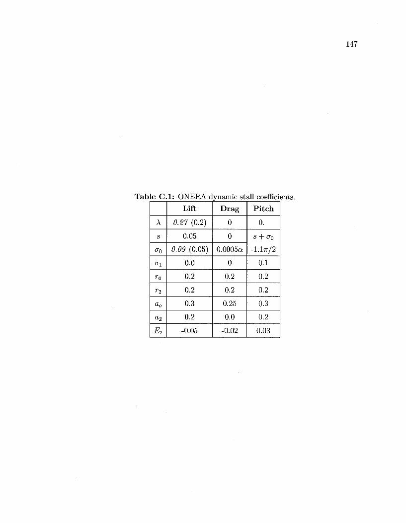
147
le C. l : ONERA d
A
s
0"o
<J\
ro
T2
a0
a2
E<2
Lift
0.27 (0.2)
0.05
0.09 (0.05)
0.0
0.2
0.2
0.3
0.2
-0.05
ynamic stall coeffici
Drag
0
0
0.0005a
0
0.2
0.2
0.25
0.0
-0.02
Pitch
0.
s + a0
-I.ITT/2
0.1
0.2
0.2
0.3
0.2
0.03
Appendix D
Changes made to the SMARTROTOR
Source Code
S809 Airfoil
SMARTROTOR uses a thin wing representation for lifting surfaces where the blade
or wing is modeled by the mean camber line. SMARTROTOR has built-in routines
to determine the mean camber line of any NACA 4-digit or 5-digit airfoil. The mean
camber line for the S809 airfoil was included in SMARTROTOR as a new airfoil
type. The mean camber line was calculated by importing the S809 airfoil surface
coordinates from [121]. The mean camber line was calculated as
Vc = tiL~2 i0-1)
As polynomial description of the camber line is required by SMARTROTOR, a fifth
order polynomial was fit to the points calculated with Equation D.l and is described
by Equation D.2.
yc = 0.5485a;5 - 1.6841a:4 + 1.6949a:3 - 0.6206a;2 + 0.0613a; + 0.0005 (D.2)
148
149
A new subroutine called S809WO was included in the file geomet-3_sp.f (lines 1344-
1372), where J is the spanwise location. The S809 airfoil can be accessed by setting
the input variable IFTYP found in the .bid input file to a value of 8. An additional
if-statement was added in geomet-3_sp.f at line 405 so that an IFTYP input of 8 will
correspond to the S809WO subroutine.
Angle of Attack Convention
The angle of attack convention for wind turbines [34] is typically in the opposite sense
of that for helicopter rotors [45]. As such, the sign in the effective angle of attack
equation (line 1449 in rescpv-3_sp.coupled2.f) was changed from a negative value (for
helicopters or wings) to a positive value (for wind turbines). This should eventually
be incorporated as an input to the code.