Multiparty Communication Complexity for Set Disjointness:

A Lower Bound

Sammy Luo, Brian Shimanuki

May 6, 2016

Abstract

The standard model of communication complexity involves two parties each starting with partialinformation on the inputs to a problem and exchanging a limited amount of information to solve theproblem jointly. In this project we investigate an extension of this model to more than two parties.In particular, we focus on an extension of the set disjointness problem to this k-party setting, wherethe parties wish to compute whether the intersection of the k input sets is nonempty. The main result

is the derivation of a lower bound of Ω((

n 1/4k

)on the randomized communication complexity for

4

DISJn,k. This is taken from Sherstov (STOC ’12).We will begin by introducing the number-on-the-forehead

)model for multiparty communication,

where each party has access to all inputs but their own. We discuss its importance and relevance tocommunication complexity theory in general. We introduce the k-party version of the set disjointnessproblem and extend a simple deterministic protocol from Grolmusz (1994) which yields an upperbound of O(log2 n+ k2n/2k) on the problem’s complexity. We then proceed to describe a series ofattempts at pushing the lower bound closer to the upper bound, illustrating the nuances of sometechniques used for working with this communication model, culminating in the stated main result.

Finally we discuss some direct product results for the problem, and compare the difficulty ofbounding the complexity of set disjointness and its cousin, the generalized inner product.

1 Introduction

1.1 Multiparty Communication

In general, communication complexity theory addresses the problem of computing a function whenno party has access to the entire input. In the typical model, two parties, Alice and Bob, have accessto inputs x ∈ X and y ∈ Y respectively, and wish to evaluate a function f : X × Y → 0, 1 oninput (x, y) using as few bits of communication as possible. The smallest number of bits that needsto be communicated in a protocol evaluating f is called the communication complexity of f . In thecase of randomized communication complexity, we allow the parties to utilize randomness and onlyrequire them to succeed with some probability 1 − ε. Results in communication complexity theoryhave many connections with other areas of complexity theory, such as circuit complexity and proofcomplexity.

It is natural to consider generalizations of the 2-party model to a setup with k ≥ 3 parties.One useful model is the so-called number-on-the-forehead model, introduced by Chandra, Furst,and Lipton [4]. In this model, k parties want to compute f(x1, . . . , xk) for some function f :X1 ×X2 × · · · ×Xk → −1, 1, where the ith party has access to all inputs except xi. (This can bethought of as the ith party has xi written on their forehead, and can see the inputs on everyoneelse’s foreheads.)

Many questions that have been thoroughly analyzed for the 2-party case remain open in thegeneral k-party setting, where lower bounds on communication complexity are much more difficultto prove. The difficulty in proving lower bounds arises from the overlap in the inputs known todifferent parties. Nevertheless, many of the methods for studying problems in the 2-party settinghave natural generalizations for tackling the corresponding multiparty versions of the problems.

1.2 Set Disjointness

One question that remains open in the k-party setting is the communication complexity of theset disjointness problem. The problem is as follows: Given input sets S1, . . . , Sk ⊆ 1, 2, . . . , n,determine whether they have empty intersection, i.e. whether S1 ∩ S2 ∩ · · · ∩ Sk = ∅. Representedas a formula, we have

n k

DISJn,k(x1, x2, . . . , xk) =j

∧=1 i

∨=1

xi

∧k,

j

∨nxij = ¬ ij

=1 =1

where xi is the vector whose jth component is 1 if j ∈ Si and 0 otherwise.gAnother formulation of DISJ comes from a comp∧ osition of∧ functions. Namely, we can defineGn,k :

0, 1n×k → −1,+1 gby Gn,k(x1, . . . , xk) = g( i xi1, . . . , i xin). Note that DISJn,k⊕is just GNORn,k .

n kAnother function of interest is the generalized inner product GIPn,k(x1, . . . , xk) = j=1 i=1 xij ,

which is GPARITYn,k . We will briefly compare these in Section 8.

The unique set disjointness problem, UDISJn,k, is the promise version of DISJn,k: we are

∧guar-

anteed that the intersection of the input sets has size either 0 or 1. The promise version of a problemcan be no harder to solve than the original problem, so giving lower bounds on the communicationcomplexity of UDISJ will give corresponding lower bounds on that of DISJ. Note that the functionUDISJn,k is a partial function, a function f whose domain dom f is a subset of X1×· · ·×Xk. Wherethe distinction is relevant, a function whose domain is the whole set will be called a total function.

The 2-party case of the set disjointness problem is well studied. A tight lower bound of n + 1is known for the deterministic communication complexity, and a tight lower bound of Ω(n) for therandomized communication complexity was shown by Kalyanasundaram and Schnitger [8].

Progress on the general k-party case has been significantly more difficult. In 1994, Grolmusz [7]proved an upper bound of O(log2 n+k2n/2k) for the deterministic complexity that remains the best

1

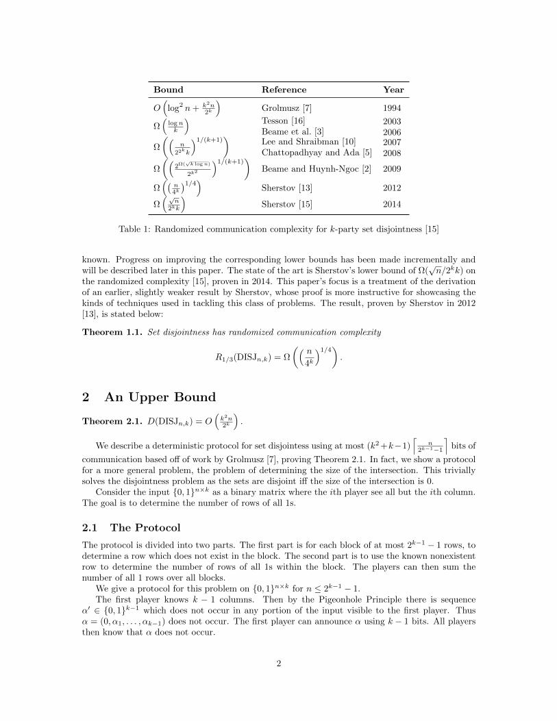
Bound Reference Year

O(

log2 n+ k2n( k

)) Grolmusz [7] 1994

2

Ω logn Tesson [16] 2003((k Beame et al. [3] 20061/(k+1) Lee and Shraibman [10] 2007

Ω nk22 k Chattopadhyay and Ada [5] 2008√ 1

Ω

(( /(k+1)2Ω( k

)logn)

)22k

) )Beame and Huynh-Ngoc [2] 2009

Ω((

n( k

)1/4)) Sherstov [13] 20124√

Ω n2k

Sherstov [15] 2014k

Table 1: Randomized communication complexity for k-party set disjointness [15]

known. Progress on improving the corresponding lower bounds has been made incrementally andwill be described later in this paper. The state of the art is Sherstov’s lower bound of Ω(

√n/2kk) on

the randomized complexity [15], proven in 2014. This paper’s focus is a treatment of the derivationof an earlier, slightly weaker result by Sherstov, whose proof is more instructive for showcasing thekinds of techniques used in tackling this class of problems. The result, proven by Sherstov in 2012[13], is stated below:

Theorem 1.1. Set disjointness has randomized communication complexity

nR1/3(DISJn,k) = Ω

(( 1

4k

) /4).

2 An Upper Bound

Theorem 2.1. D(DISJn,k) = O(k2n2k

).

We describe a deterministic protocol for set disjointess using at most (k2 +k−1)⌈

n bits2k−1 of−1

communication based off of work by Grolmusz [7], proving Theorem 2.1. In fact, we show a proto

⌉col

for a more general problem, the problem of determining the size of the intersection. This triviallysolves the disjointness problem as the sets are disjoint iff the size of the intersection is 0.

Consider the input 0, 1n×k as a binary matrix where the ith player see all but the ith column.The goal is to determine the number of rows of all 1s.

2.1 The Protocol

The protocol is divided into two parts. The first part is for each block of at most 2k−1 − 1 rows, todetermine a row which does not exist in the block. The second part is to use the known nonexistentrow to determine the number of rows of all 1s within the block. The players can then sum thenumber of all 1 rows over all blocks.

We give a protocol for this problem on 0, 1n×k for n ≤ 2k−1 − 1.The first player knows k − 1 columns. Then by the Pigeonhole Principle there is sequence

α′ ∈ 0, 1k−1 which does not occur in any portion of the input visible to the first player. Thusα = (0, α1, . . . , αk 1) does not occur. The first player can announce α using k− − 1 bits. All playersthen know that α does not occur.

2

Given an α which all players know does not occur as a row, we show how to compute the numberof all 1 rows. Without loss of generality, α is of the form (0, . . . , 0, 1, . . . , 1) since the players canrenumber themselves according to α. Define yi as the number of rows in the input of the form(0, . . . , 0, 1, . . . , 1) starting with i 0s. Now supposing α contains l 0s, yl = 0 is the number of timesα occurs. For each i < l, using k bits, the ith player announces zi, the number of rows of the form(0, . . . , 0, ∗, 1, . . . , 1) where the ∗ occurs at the ith column and∑is unknown∑to the ith player. Notethat zi = yi + yi+1. Each player can then privately compute i even zi − i odd zi = y0 + yl = y0.This is the number of all 1 rows.

2.2 Cost Analysis

For each of the⌈

n2k−1−1

⌉blocks, the protocol uses k − 1 bits to determine α, and uses k bits to

determine zi for 0 ≤ i < l. Since l ≤ k, we have this is a total of⌈

n2k−1−1

⌉((k − 1) + k · k) =

(k2 + k − 1)⌈

n bits2k−1−1

⌉as claimed.

3 Preliminaries

For simplicity, we define Boolean functions to use the range −1,+1 with −1 corresponding totrue. We let [m] denote the set 1, . . . ,m. Finally, let f g denote the composition of functions fand g, that is, for functions f : −1,+1n → −1,+1, g : X → −1,+1 we define the compositionf g : Xn → −1,+1 by (f g)(x1, . . . , xn) = f(g(x1), . . . , g(xn)).

3.1 Cylinder Intersections

In 2-party communication complexity, we can model protocols as a decision tree with nodes markedby rectangles. In multiparty communication, we use a generalized analogue, which are called cylinderintersections, as introduced by Babai, Nisan, and Szegedy [1].

Definition 3.1 (Cylinder Intersections). A k-dimensional cylinder intersection is a function χ :k

X1 × X2 × · · · × Xk → 0, 1 of the form χ(x1, . . . .xk) = i=1 χi(x1, . . . , xi−1, xi+1, . . . , xk) withχi : X1 × · · · ×Xi X X 0, 1 .−1 × i+1 × · · · × k →

∏Thus a k-dimensional cylinder is the product of k functions which do not depend on one of the k

coordinates. In the forehead model, this corresponds to a player not knowing the number on his ownforehead. At any point in the protocol, what each player knows is independent of his own number.

Note that when k = 2, we get that χ(x1, x 1 12) = χ1(x2)χ2(x1) = [x2 ∈ S1]1

· [x1 ∈ S2] =[(x1, x2) ∈ S2 × S1] for some S1, S2 ⊆ [n]. This is exactly the indicator for a rectangle.

Recall that in the case of a 2-party protocol, we can divide the input space into rectangles.More explicitly, if Π : X × Y

c→ −1,+1 is a deterministic protocol with cost c, then X × Y can

be divided into 2 (possibly empty) disjoint rectangles which lead to the 2c possible transcripts.The same reasoning on cylinder intersections generalizes to the following proposition in the k-partymodel.

Proposition 3.2. Let Π : X1 × · · · × Xk be a deterministic k-party communication protocol withcost c. Then

2c

Π = aiχii=1

for some cylinder intersections χ1, . . . , χ

∑2c with pairwise disjoint support and some coefficients

a1, . . . , a2c ∈ −1,+1.

3

Now a randomized protocol with cost c is a probability distribution on deterministic protocolsof cost exactly c. So the following corollaries are directly implied by Proposition 3.2.

Corollary 3.3. Let F be a (possibly partial) Boolean function on X1×· · ·×Xk. If Rε(F ) = c, then

ε|F (x1, . . . , xk)−Π(x1, . . . , xk)| ≤1− ε

, (x1, . . . , xk) ∈ domF,

|Π(x1, . . . , xk)| ≤ 1, (x ,

− 1 . . . , xk)1 ε

∈ X1 × · · · ×Xk,

c

where Π =∑χ aχχ is a linear combination of cylinder intersections with

∑|aχ| ≤ 2

χ .1−ε

Corollary 3.4. Let |pi be a randomized k-party protocol with domain X1 ×X2 × · · · ×Xk and costc. Then

P [Π(x1, . . . , xk) = −1] ≡∑

aχχ(x1, . . . , xk)χ

on X1 × · · · ×Xk, where each χ is a cylinder intersection and∑χ |aχ| ≤ 2c.

3.2 Fourier Transform

We define the multidimensional Fourier transform on the Boolean hypercube −1,+1n.

Definition 3.5 (Fourier Transform). Define χS(x) =∏i S xi for S ∈ [n]. Note that these form∈

an orthonormal basis over the vector space of real functions over the Boolean hypercube. Everyfunction∑ ˆ ˆφ : −1,+1n → R has a unique representation φ(x) =

∑S [n] φ(S)χS(x), where φ(S) =

2−n∈

x 1,+1 n φ(x)χS(x) are called the Fourier coefficients of φ.∈−

3.3 Polynomial Approximation

Another useful technique, closely related to the consideration of the Fourier transform of a functionφ, is that of approximating φ by a low-degree polynomial.

Definition 3.6. For a partial function φ : X → R and a nonnegative real ε, the ε-approximatedegree of φ, denoted degε(φ), is defined as the least degree of a real polynomial p with

|φ(x)− p(x)| ≤ ε if x ∈ domφ,

|p(x)| ≤ 1 + ε otherwise.

Define E(φ, d) to be the smallest ε such that degε(φ) ≤ d.

Notice that if φ is a partial Boolean function, then a polynomial p that ε-approximates anyextension of φ to a total Boolean function f also gives an ε-approximation to φ, since |p(x)| ≤|f(x)− p(x)|+ |f(x)| ≤ ε+ 1 when x ∈/ domφ.

We will make use of a few results on approximate degrees. The first is a result due to Sherstov[12], relating approximate degree to an inequality involving a function with no low-order Fouriercoefficients:

Theorem 3.7. Given a partial real-valued function φ on −1,+1n, we have degε(φ) > d if andonly if there exists ψ : −1,+1n → R such that

x

∑φ(x)ψ(x)

domφ

−∑

|ψ(x)| − ε‖ψ‖1 > 0,∈ x∈/domφ

ˆand ψ(S) = 0 for |S| ≤ d.

4

Let ANDn be the promise version of the function ANDn, so its domain consists of sets of inputsat most one of which is false. We have the following bound proven by Nisan and Szegedy [11]:

Theorem 3.8.deg1/3(ANDn) = Θ(

√n),

deg1/3(ANDn) = Θ(√n).

Corollary 3.9.deg1/3(NORn) = deg1/3(ANDn) = Θ(

√n).

The proof of Theorem 3.7 is an application of LP duality; see [12]. Theorem 3.8 follows from asimple analytic result that gives a Θ(

√n) lower bound on the degree of a polynomial given a large

derivative at one point and some bounds on its values at n consecutive integers; see [11]. Corollary 3.9follows from the bijection NORn(x1, . . . , xn) = ANDn(1−x1, . . . , 1−xn), which doesn’t change thedegree.

The importance of Theorem 3.8 to the disjointness problem comes from the observation that for

any m, r, k we have DISJmr,k = ANDm DISJr,k and UDISJmr,k = ANDm UDISJr,k. Similarly,we take notice of Corollary 3.9 because DISJn,k is equivalent to GNOR

n,k .

4 Discrepancy

In the case of randomized communication complexity, our analysis needs some refinement beyondthe direct use of cylinder intersections. The concept of discrepancy is an important tool that servesto generalize the use of monochromatic rectangles in the 2-party case, or of cylinder intersections inthe k-party case, to the analysis of a randomized protocol.

In the 2-party setting, the discrepancy of a (total) function f : X × Y → −1,+1 with respectto a probability distribution P is defined as

discP (f) = maxR=S×T

|P (R ∩ f−1(1))− P (R ∩ f−1(−1))|

= max

∣∣∣∣ ∑∣∣ f(x, y)P (x, y)χR(x, y)R

(x,y)∈X×Y

∣∣∣,

whereR ranges over all rectangles and χR is the indicator function for the

∣∣∣rectangleR (i.e. χR(x, y) =

1 if (x, y) ∈ R and χR(x, y) = 0 otherwise).The last expression for discrepancy above extends well to the k-party setting by simply replacing

rectangles by general cylinder intersections. We have, for a total function F ,

discP (F ) = max

∣∣∣ ∑F (x)P (x)χ(x)

χx∈X1×X2×···×Xk

∣∣∣,

where χ ranges over all cylinder intersections.

∣∣ ∣∣We can extend this definition to a partial function F by setting

discP (F ) =∑

P (x) + maxχ

x∈/domF

∣∣F (x)P (x)χ(x) .

x∈

∑domF

∣∣We define the overall discrepancy to be disc(F ) =

∣∣ ∣∣minP discP (F ), the least

∣∣discrepancy over all

possible probability distributions.

5

Intuitively, discrepancy is a measure of how strongly a function correlates with a particularcylinder intersection, and computing it plays a similar role to finding a Fourier coefficient of maximalmagnitude.

It has been long established [6] for the 2-party model that low discrepancy leads to lowerbounds on communication complexity. Namely, for any function F : 0, 1n → −1,+1, we have2Rε(F ) ≥ 1−2ε . This also holds in the k-party model as well as in the partial functions extension.disc(F )

Sherstov [13] proves the following theorem.

Theorem 4.1 (Discrepancy Method). Let F be a (possibly partial) Boolean function on X1×· · ·×Xk.Then

2Rε(F ) 1− 2ε≥ .disc(F )

A stronger technique is to find a function Ψ which is highly correlated with F but has lowcorrelation with all cylinder intersections. This method is referred to as the generalized discrepancymethod, which is proved in [13].

Theorem 4.2 (Generalized Discrepancy Method). Let F : X1×· · ·×Xk → −1,+1 be a (possiblypartial) Boolean function. Then for every nonzero Ψ : X1 × · · · ×Xk → R,

2Rε(F ) 1− ε≥maxχ |〈χ,Ψ〉|

∑x∈domF

F (x)Ψ(x)−∑

x6∈domF

|Ψ(x)| − εΨ

1− ε‖ ‖1

,

where maxχ is over cylinder intersections χ.

We have the following useful upper bound on discrepancy given in [13], which has a very simpleproof:

Proposition 4.3. For a (total) function F : X × Y → −1, 1 and a probability distribution P onX × Y , define Φ to be the |X| × |Y | matrix Φ = [F (x, y)P (x, y)]x∈X,y∈Y . Then

discP (F ) ≤ ‖Φ‖√|X||Y |.

Here ‖Φ‖ denotes the spectral norm of Φ as a linear map, i.e. ‖Φ‖ = maxx6=0‖Φx‖ , where x‖x‖

ranges over nonzero vectors in RX .

Proof. We have discP (F ) = maxR

∣(x,y) X Y F (x, y)P (x, y)χR(x, y) . Pick χ∈ × R attaining this

maximum. Say R = S × T , and let 1S , 1T be the indicator functions for

∣S, T respectively, and let

v , e

∑S v

∣RYT b the corresponding indicator

∣vectors in RX , respectively. Then

∣∣

discP (F ) =

∣∣∣∣ ∑∣∣ F (x, y)P (x, y)1S(x)1T (y)

∣∣∣∣∣ = |vT · (ΦvS) | ≤ ‖vT ‖‖ΦvS‖(x,y)∈X×Y

≤ ‖vT ‖‖Φ‖‖vS‖ ≤ ‖Φ‖

∣√|X||Y |.

Here we have used Cauchy-Schwarz as well as the definition of the spectral norm.

Sherstov uses this to prove a general discrepancy-type result relevant to the analysis of an XOR ofm copies of UDISJn,k. Before stating this result, we make a few definitions to simplify our notation.Specifically, when X1, . . . , Xr are any 0, 1-matrices or vectors with n rows, let D(X1, . . . , Xr) = −1if for 1 ≤ j ≤ n, one of the Xi has a 0 in row j, and let D(X1, . . . , Xr) = 1 otherwise. So whenx1, . . . , xk are vectors, we have D(x1, . . . , xk) = DISJn,k(x1, . . . , xk).

6

Let Un be the uniform distribution on the set 0, 1n of 0, 1-vectors in Rn, and let µn,k be theuniform distribution on n × k 0, 1-matrices such that exactly one row consists of all ones, thusadmitting at most one coordinate at which disjointness can fail. Hence the support of Un × µn,k−1,viewed as a distribution on sets of k vectors, is contained in the domain of UDISJn,k.

Finally, recall that for a distribution P on a set X, the notation x ∼ P means that x ∈ X is arandom variable∑distributed according to P . For any function F , the expectation with respect to Pis Ex∼P F (x) = x (∈X P (x)F x).

Now, define

m

Γk(n1, n2, . . . , nm) = maxχ

∣∣∣ E χ D(xi,W i) ,(x1,W 1),...,(xm,Wm)

[·i

∏=1

]∣∣∣for any positive integers n i i

1, . . . , nm. Here

∣∣(x ,W ) ∼ Uni

∣∣× µni,k, and χ ranges over cylinder

intersections of dimension k + 1 on X × · · ·X = (0, 1n1+ +1 k+1

··· nm)k+1, where Xj consists of thejth columns of each (xi,W i). That is, we can view the overall distribution µ(m) of all the (xi,W i) asa distribution over (k+ 1)-tuples of collections of m vectors (v1, . . . , vm) ∈ 0, 1n1 × · · · × 0, 1nm ..

The connection with the discrepancy of unique disjointness becomes clear when we notice thatm

Γk(n1, n2, . . . , nm) = discµ(m)(F ), where F = i=1D(xi,W i), viewed as a function on X1+

×· · ·X 1

+1 = (0, 1nk···+nm)k+1. So F =

i−1 if

isfy disjointness. Each parameter (x ,W i) corresp

∏and only if an odd number of the (xi,W i) sat-onds to an instance of UDISJ, so F computes the

XOR of m instances of unique disjointness. That is,

Γk(n1, n2, . . . , nm) = discµ(m)(UDISJn1,k+1⊕ · · · ⊕UDISJnm,k+1).

Sherstov [13] gives the following bound:

Theorem 4.4. For all positive integers n1, n2, . . . , nm and k,

(2k 1)mΓk(n1, n2, . . . , nm)

−≤ √ .n1n2 · · ·nm

The proof given in [13] uses induction on k, reducing to a smaller-dimensional cylinder intersectionthrough use of conditional independence and bounding of the expectations that arise. It is instructiveto look at the proof of the base case, expanding on the proof sketch that Sherstov gives.

Proposition 4.5. For all positive integers n1, n2, . . . , nm,

1Γ1(n1, n2, . . . , nm) ≤ √ .

n1n2 · · ·nm

Proof. Note that for k = 1, each W i in the definition of Γk reduces to a vector with exactly onenonzero component. Thus, W i is effectively a uniformly random integer ji ∈ 1, 2, . . . , ni. ThenD(xi,W i) = −1 if and only if xiji , the jith entry of xi, is 0. So

m

Γ1(n1, n2, . . . , nm) = disc 1+xijiµ(m)

(∏(−1)

i=1

).

As in Proposition 4.3, then, we construct a matrix of the form Φ = [F (x, y)P (x, y)]x∈X,y∈Y , wherex = (x1, . . . , xm) ∈ X = 0, 1n1 × · · · × 0, 1nm and y = (j1, . . . , jm) ∈ Y = [1, n1]

1

× · · · × [1, nm].

So P (x, y) = ∏mi=1 ni2

nifor all x, y, and F (x, y) =

∏mi=1(−1)1+xiji . Since F · P is a product of m

7

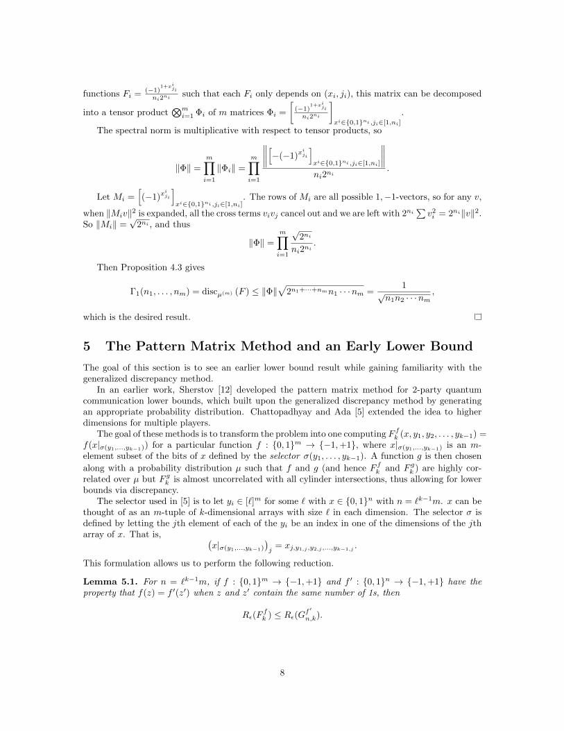
functions Fi = (−1)1+xiji

nisuch that each Fi only dep[ends on (xi, ji), this matrix can be decomposedni2

into a tensor product⊗ i

m (i=1 Φi of m matrices Φi = − 1+x

1) ji

ni2ni

]xi∈0,1ni ,ji∈[1,ni]

.

The spectral norm is multiplicative with respect to tensor products, so

‖Φ‖ =m∏i=1

‖Φi‖ =m∏i=1

∥∥∥∥[−(−1)xiji

]xi∈0,1ni ,ji∈[1,ni]

∥∥∥∥.

ni2ni

Let Mi =[(−1)x

iji

]. The rows of Mi are all possible 1,−1-vectors, so for any v,

xi

2∈0,1ni ,ji∈[1,ni]

when ‖Miv‖ n 2 n 2

So Mi =√ is expanded, all the cross terms v j cancel out and we are left with 2 i

∑v = 2 i

iv i ‖v‖ .‖ ‖ 2ni , and thus

‖Φ‖ =m∏i=1

√2ni

.ni2ni

Then Proposition 4.3 gives

Γ1(n1, . . . , nm) = discµ(m) (F ) ≤ ‖Φ‖√

2n1+···+nmn1 · · ·nm =1

√ ,n1n2 · · ·nm

which is the desired result.

5 The Pattern Matrix Method and an Early Lower Bound

The goal of this section is to see an earlier lower bound result while gaining familiarity with thegeneralized discrepancy method.

In an earlier work, Sherstov [12] developed the pattern matrix method for 2-party quantumcommunication lower bounds, which built upon the generalized discrepancy method by generatingan appropriate probability distribution. Chattopadhyay and Ada [5] extended the idea to higherdimensions for multiple players.

fThe goal of these methods is to transform the problem into one computing Fk (x, y1, y2, . . . , yk−1) =f(x|σ(y1,...,yk 1)) for a particular function f : 0, 1− m → −1,+1, where x|σ(y1,...,yk−1) is an m-element subset of the bits of x defined by the selector σ(y1, . . . , yk 1). A function g is then chosen−

f galong with a probability distribution µ such that f and g (and hence Fk and Fk ) are highly cor-grelated over µ but Fk is almost uncorrelated with all cylinder intersections, thus allowing for lower

bounds via discrepancy.The selector used in [5] is to let yi ∈ [`]m for some ` with x ∈ 0, 1n with n = `k−1m. x can be

thought of as an m-tuple of k-dimensional arrays with size ` in each dimension. The selector σ isdefined by letting the jth element of each of the yi be an index in one of the dimensions of the jtharray of x. That is, (

x|σ(y1,...,yk−1) = xj,yj 1,j ,y2,j ,...,yk−1,j.

This formulation allows us to perform the follo

)wing reduction.

Lemma 5.1. For n = `k−1m, if f : 0, 1m → −1,+1 and f ′ : 0, 1n → −1,+1 have theproperty that f(z) = f ′(z′) when z and z′ contain the same number of 1s, then

fRε(Fk ) ≤ f ′Rε(Gn,k).

8

Proof. There are functions Γi : [`]m → 0, 1n, namely the bitmask for the coordinate in the ithf f ′dimension of each array, such that Fk (x, y1, . . . , yk 1) = Gn,k(x,Γ1(y1), . . . ,Γk 1(y ))− − k−1 for all

fx, y1, . . . , yk can−1. Thus players for Fk privately convert their inputs and use the protocol forf ′Gn,k.

Remark. The functions f = NORm and f ′ = NORn satisfy the conditions of this lemma, and willlead to bounds on DISJn,k.

fWe bound the complexity of Fk in terms of discrepancy.

Lemma 5.2. Let µ be a probability distribution on −1,+1n m k 1

m and let λ be the probability distributionµ(x )

on −1,+1 ×([`] ) − defined from µ as λ(x, y1, . . . , yk−1) =|σ(y ,...,y1 k− )1

`m(k−1)2n−m. If f : −1,+1m →

−1,+1 satisfies Ex∼µ f(x)χS(x) = 0 for all |S| < d and some positive integer d, then

(discλ(F fk )

)2k−1

≤(k−1)m∑j=d

((k − 1)m

j

)(22k−1−1

j

`− 1

).

k

Remark. For `− 1 ≥ 22 (k−1)emd and d > 2, we have discλ(F fk ) ≤ 1

k2d/2 −1 .

Proof sketch. The full proof can be found in [5]. The main idea is to compute the discrepancy withrespect to an arbitrary cylinder intersection and bound it using algebraic and Fourier properties.

We have the discrepancy with respect to cylinder intersection χ is

f fdiscλ(Fk ) =

∣∣∣∣ ∑∣∣ Fk (x, y1, . . . , yk 1)χ(x, y1, . . . , yk 1)λ(x, y1, . . . , y )− − k−1

x,y1,...,yk−1

∣∣∣∣=

∣∣∣∣ E fFk (x, y1, . . . , yk 1)χ(x, y1, . . . , yk 1)µ(xx,y

− − y1,...,y −

∣,...,y

|σ( k 1))1 k−1

∣∣.

With repeated applications of the triangle inequality and the Cauchy-Schwartz ine

∣∣∣quality, this

can be transformed to

( 2k−1

f fdiscλ(Fk ))

≤ E E Fk (x, y1,u1 , . . . , yk 1,uk 1)µ(x σ(y ,...,y )) .

y k0,y1,1,...,y

1 11, k−1,0,yk x

u∈

∏− −

−1,1

∣∣0,1k−1

| −

∣∣∣∣ ∣∣ ∣Let r = the follo

∣∑i |yi,0 ∩ yi,1|. We make wing claims, of which the proofs can be found in [5].

∣∣

Claim 5.3. ∣∣∣∣E ∏f | ∣∣∣∣ ≤ (2k 1∣ −

F (x, y , . . . , y )µ(x )∣ 2 −1)r∣ k 1,u1 k 1,uk 1x− − σ(y1,...,yk−1) .

u∈0,1k−1

This follows from µ being a probability distribution.

∣Claim 5.4. If r < d,∣∣∣∣∣E ∏

f∣ Fk (x, y1,u1, . . . , yk 1

)µ(x− |σ(x

−1,uk y1,...,yk−1)) = 0.

u∈0,1k−1

∣∣∣∣∣∣

9

ˆThis claim can be proved using the Fourier theoretic properties of f(S) = 0 for |S| < d.Together with some probability and combinatorial identities, the bounds made in these claims

can be used to obtain the theorem.

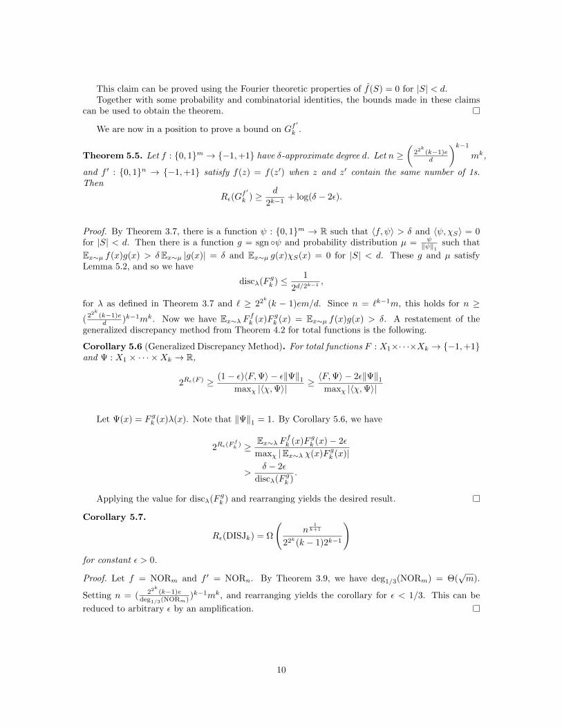
f ′We are now in a position to prove a bound on Gk .

m → − ≥(

k22 (k−1)eTheorem 5.5. Let f : 0, 1 1,+1 have δ-approximate degree d. Let n d

)k−1

mk,

and f ′ : 0, 1n → −1,+1 satisfy f(z) = f(z′) when z and z′ contain the same number of 1s.Then

Rε(Gf ′

k ) ≥ d+ log(δ 2

2k−1− ε).

Proof. By Theorem 3.7, there is a function ψ : 0, 1m → R such that 〈f, ψ〉 > δ and 〈ψ, χS〉 = 0for |S| < d. Then there is a function g = sgn ψ and probability distribution µ = ψ such that‖ψ‖E

1

x µ f(x)g(x) > δ Ex µ |g(x)| = δ and Ex µ g(x)χS(x) = 0 for |S| < d. These g and µ satisfy∼ ∼ ∼Lemma 5.2, and so we have

g 1discλ(Fk ) ≤

2 k ,d/2 −1

for λ as defined in Theorem 3.7 and ` ≥ 22k(k − 1)em/d. Since n = `k−1m, this holds for nk

22 (k

≥( −1)e f)k−1mk. Now we have E g

x E∼λ Fk (x)Fk (x) = x µ f(x)g(x) > δ. A restatement of thed ∼generalized discrepancy method from Theorem 4.2 for total functions is the following.

Corollary 5.6 (Generalized Discrepancy Method). For total functions F : X1×· · ·×Xk → −1,+1and Ψ : X1 × · · · ×Xk → R,

2Rε(F ) (1− ε)〈F,Ψ〉 − ε‖Ψ‖≥ 1

maxχ |〈χ,Ψ〉|≥〈F,Ψ〉 − 2ε‖Ψ‖1

maxχ |〈χ,Ψ〉|

gLet Ψ(x) = Fk (x)λ(x). Note that ‖Ψ‖1 = 1. By Corollary 5.6, we have

f

2Rε(F )kE f g

≥ x λ Fk (x)Fk (x)− 2ε∼

maxχ |Ex∼λ χ(x)F gk (x)|

>δ − 2ε

g .discλ(Fk )

gApplying the value for discλ(Fk ) and rearranging yields the desired result.

Corollary 5.7.

Rε(DISJk) = Ω

(1

n k+1

22k(k − 1)2k−1

)for constant ε > 0.

Proof. Let f = NORm and f ′ = NORn. By Theorem 3.9, we have deg1/3(NORm) = Θ(√m).

k22 (kSetting n = ( −1)e )k 1mk, and rearranging yields the corollary for ε < 1/3. This can bedeg )

−1/3(NORm

reduced to arbitrary ε by an amplification.

10

6 The Main Theorem

The key to Sherstov’s proof of Theorem 1.1 is the following bound relating approximate degree torandomized communication complexity:

Theorem 6.1. Let f be a partial Boolean function on −1,+1n, and let F = f UDISJr,k. Forany ε, δ ≥ 0, let c = Rε(F ) be the randomized communication complexity with error ε of F as ak-party communication problem, and let d = degδ(f). Then we have

2c√

≥ (δ ε(1 + δ))

(d− r

d

2ken

).

Given this theorem, the proof of Theorem 1.1 is straightforward:

Proof of Theorem 1.1. By Theorem 3.8, for some c > 0 we have deg1/3(ANDm) > c√m for all m.

Since UDISJmr,k = ANDm UDISJr,k, applying Theorem 6.1 with ε = 1/5, δ = 1/3, n = m, r =

4k+2m/c2, f = ANDm gives d ≥ c√m and

R1/5(UDISJmr,k) ≥ log

(1/15 + d log

(d2k+2

√m

c2kem

))≥ Ω

(√m log

(4

e

))= Ω(

√m).

Replacing√ R1/5 by R1/3 should only change the bound by a constant factor. Now, setting m ≈c2n/4k+2 gives mr ≈ n, so

R1/3(DISJn,k) ≥ R1/3(UDISJn,k) ≥ Ω( n

4k

)1/4

,

as claimed.

We present two proofs of Theorem 6.1 given by Sherstov in [13], rearranged and clarified here tohighlight the motivation behind each step.

6.1 Primal Proof

The first proof is described as “primal” because, unlike previous work on results of this nature, itdoes not rely on switching to the dual view of the problem. The method used in this proof resurfacesin the proofs of direct product results later in the paper.

Primal proof of Theorem 6.1. The idea of this proof is to construct a low-degree polynomial approx-imating f given a protocol attaining communication cost c = Rε(F ).

As in Section 4, we think of F (X1, . . . , Xn) in the communication protocol setting as a functionon k inputs Y1, . . . , Yk, where Yj ∈ 0, 1r×n consists of the jth columns of each Xi. Then by 3.3,F is approximated by a linear combination Π = χ aχχ of k-dimensional cylinder intersectionsχ(Y1, . . . , Yk) = χ(X1, . . . , Xn), with

∑χ |aχ| ≤ 2c/

∑(1− ε).

We want to convert this approximation into an approximation of f by a low-degree polynomial.To translate the approximation from F to f , we will introduce an operator M sending each functionG : (0, 1r×k)n → −1,+1 to a function MG : 0, 1n → −1,+1. Since F (X1, . . . , Xn) =f(UDISJr,k(X1), . . . ,UDISJr,k(Xn)), M will be an averaging operator that retains information aboutthe values of UDISJr,k on the inputs.

Let µ = Ur × µr,k 1, and let µ ,− +1 µ−1 be the probability distributions that µ induces onUDISJ−1

r,k(−1),UDISJ−1r,k(1) respectively. So, for example, µ+1(X0) is the probability of choosing

X = X0 when sampling X according to µ conditioned on UDISJr,k(X) = 1. Let X = (x,W ) ∼ µ.

11

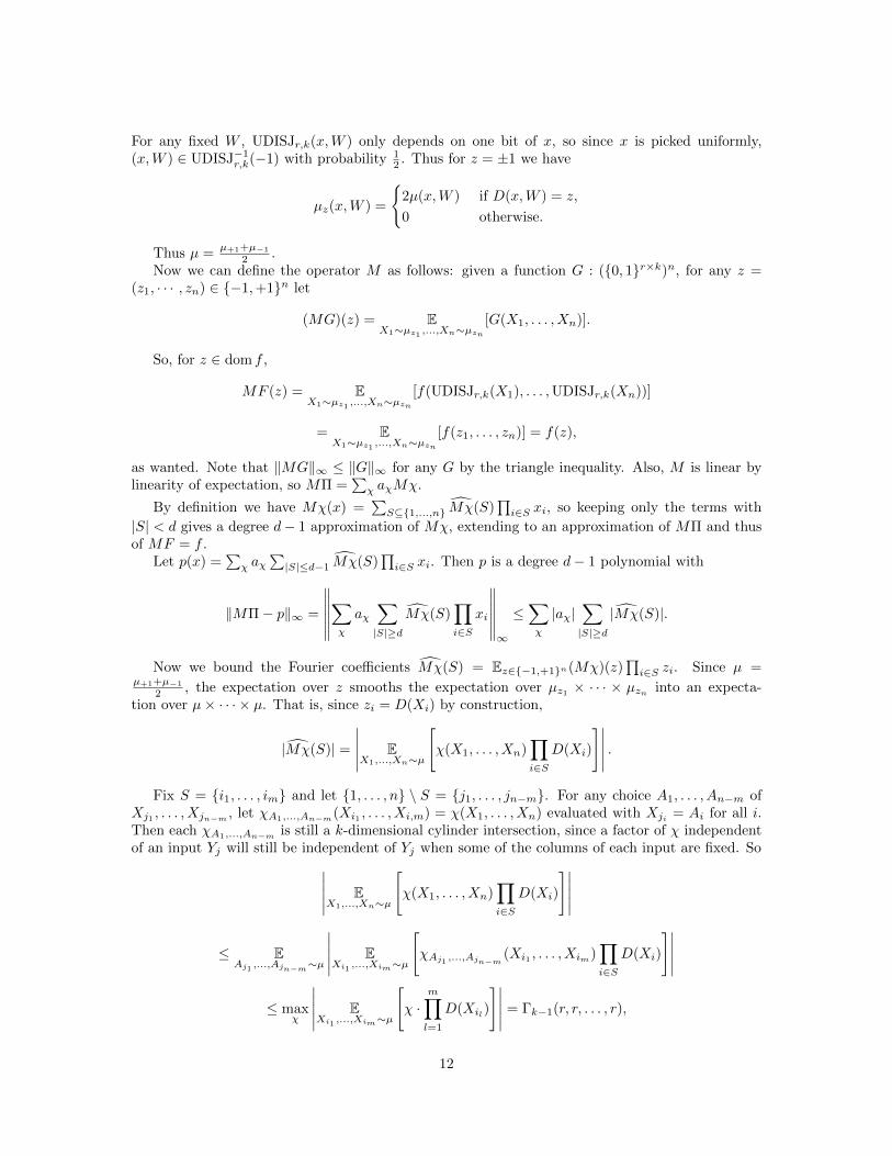
For any fixed W , UDISJr,k(x,W ) only depends on one bit of x, so since x is picked uniformly,(x,W ) ∈ UDISJ−1

r,k(−1) with probability 1 . Thus for z = ±1 we have22µ(x,W ) if D(x,W ) = z,

µz(x,W ) =0 otherwise.

µThus µ = +1+µ−1 .2Now we can define the operator M as follows: given a function G : (0, 1r×k)n, for any z =

(z1, · · · , zn) ∈ −1,+1n let

(MG)(z) = E [G(X1, . . . , Xn)].X1∼µz ,...,Xn1

∼µzn

So, for z ∈ dom f ,

MF (z) = E [f(UDISJr,k(X1), . . . ,UDISJr,k(Xn))]X1∼µz ,...,Xn1

∼µzn

= E [f(z1, . . . , zn)] = f(z),X1∼µz ,...,Xn z1

∼µ n

as wanted. Note that ‖MG‖ ≤ ‖G‖ for any G by the triangle inequality. Also, M is linear by∞ ∞linearity of expectation, so MΠ = χ aχMχ.

By definition we have Mχ(x)

∑=∑S⊆1,...,n Mχ(S) i∈S xi, so keeping only the terms with

|S| < d gives a degree d− 1 approximation of Mχ,of

extending

∏to an approximation of MΠ and thus

MF = f .Let p(x) =

∑χ aχ

∑S d 1 Mχ(S)

∏i S xi. Then p is a degree d− 1 polynomial with| |≤ − ∈

‖MΠ− p‖ =

∥∥∥∥ M

∥∑aχ∑ ∥

χ(S)∏

xi∥∥ ≤

∑|aχ|

∑|Mχ(S)∞

χ |S|≥d i∈S χ

|.|S|≥d∞

Now we bound the Fourier

∥∥coefficients M

∥∥χ(S) = Ez 1,+1 n(Mχ)(z)∈−

∏i∈S zi. Since µ =

µ+1+µ−1 , the expectation over z smooths the expectation over µz2 1× · · · × µzn into an expecta-

tion over µ× · · · × µ. That is, since zi = D(Xi) by construction,

|Mχ(S)| =

∣∣ [∣ E χ(X1, . . . , Xn)∣.

X1,...,Xn∼µi

∏D(Xi)

∈S

]∣∣Fix S = i

∣∣ ∣ 1, . . . , i

m and let 1, . . . , n \ S = j1, . . . , jn m. For any

∣choice A1, . . . , A− n−m of

Xj1 , . . . , Xjn m, let χA1,...,An m

(Xi− − 1, . . . , Xi,m) = χ(X1, . . . , Xn) evaluated with Xji = Ai for all i.

Then each χA1,...,An mis still a k-dimensional cylinder intersection, since a factor of χ independent−

of an input Yj will still be independent of Yj when some of the columns of each input are fixed. So∣∣∣∣∣ E χ(X1, . . . , Xn) D(Xi)X1,...,Xn∼µ

[i

∏∈S

]∣∣∣∣≤ E E χAj ,...,Aj (Xi1 , . . . , X

∣im) D(Xi)

A n mj ,...,Aj µ Xi ,...,X 1

i µ1 n−m∼

∣∣ [ ∏ ]∣∣∣∣ 1 m∼ −i∈S

∣∣∣≤ max

∣∣∣∣∣ E

[χ ·∏m

D(Xi

∣χ Xi ,...,Xim µ

1∼ l

)l=1

]∣∣∣∣∣ = Γk−1(r, r, . . . , r),

12

(2k−1 1)mwhere Γk 1 has m = |S| inputs of r. By Theorem 4.4 we have Γk 1(r, r, . . . , r) ≤ −− − rm/2

≤(2k−1√

m

r

). So,

‖MΠ− p‖∞ ≤∑χ

|aχ|∑ 2k−1

|Mχ(S)| ≤∑χ

|aχ||S|≥d |S

∑|≥d

(√r

)|S|

≤ 2c

1− ε

n∑m=d

(n

m

)(2k−1

√m

r

).

When 2kend√

c

1,r≤ applying binomial sum bounds then gives ‖MΠ− p‖∞ ≤ 2

1−ε

(2kend√r

)d. Other-

wise, replace p by 0. Then ‖MΠ‖∞ ≤ ‖Π‖∞ ≤ 1 by the specifications of the approximation of F1−ε

‖ − ‖ ≤ 2cby Π, so we still have MΠ p ∞ 1−ε

(2kend√r

)d. Hence, E(MΠ, d− 1) ≤ 2c

1−ε

(2kend√

d

r

).

So, for some polynomial p of degree at most d− 1, we have, for x ∈ dom f ,

ε|f(x)− p(x)| ≤ |f(x)−MΠ(x)|+ ‖MΠ− p‖∞ ≤ + E(MΠ, d .− ε

− 1)1

For x ∈/ dom f , we have

1|p(x)| ≤ ‖MΠ‖ +∞ ‖MΠ− p‖∞ ≤1− ε

+ E(MΠ, d− 1) =ε

+ E(MΠ, d1− ε

− 1) + 1.

Soε

E(f, d− 1) ≤1− ε

+ E(MΠ, d− 1) ≤ ε

1− ε+

2c

1− ε

(2ken

d√

d

r

).

Since degδ(f) = d, we must have δ < E(f, d− 1) ≤ ε1−ε + 2c

1−ε

(2kend√

d

r

), which rearranges to the

bound desired.

6.2 Dual Proof

Unlike previous analyses using the generalized discrepancy method and pattern matrix techniques,Sherstov gives an explicit probability distribution, for which a selector can be applied which exploitsconditional properties of the distribution. Namely, the probability distribution acts on a subspace of(0, 1r×k)n, which allows a selector to work which would not have worked on the entire (0, 1r×k)n

space.With this selector, we construct our highly correlated function Ψ and then proceed to bound its

inner product with all k-dimensional cylinder intersections. These allow us to use the generalizeddiscrepancy method to place a bound on F .

Dual proof of Theorem 6.1. We begin by dividing the input (0, 1r×k)n into n blocks of 0, 1r×k.Our selector will select one bit from each block.

Consider the same probability distribution µ = UR × µr,k−1 on the domain of UDISJr,k. Letd = degδ(f). By Theorem 3.7, there is a function ψ : −1,+1n → R which satisfies∑

f(x)ψ(x) ψ(x) > δ,x

−∈dom f x6∈

∑dom f

| |

‖ψ‖1 = 1,

ψ(S) = 0, |S| < d.

13

Recall that each element A from our probability distribution µ has at most one row which cancontain all 1s, namely the unique row of all 1s in the last k − 1 columns as generated by µr,k−1.Thus if we view the columns of A as (x, y1, . . . , yk−1), the columns y1, . . . , yk can act as a selector−1

for the first column in that x|S(y1,...,yk 1) = xj where j is the row of all 1s in y1, . . . , yk− −1.

Define Ψ : (0, 1r×k)n → R by

n

Ψ(X1, . . . , Xn) = 2nψ(DISJr,k(X1), . . . ,DISJr,k(Xn))∏

µ(Xi)i=1

for blocks Xi.Since µ distributes equally onto UDISJ−1

r,k(−1) and UDISJ−1r,k(+1),

‖Ψ‖1 = 2n E ψ(x) = 1.x∈−1,+1n

| |

Similarly,∑F (X1, . . . , Xn)Ψ(X1, . . . , Xn)

domF

−∑

|Ψ(X1, . . . , Xn)| =∑

f(x)ψ(x)−∑

|ψ(x)

domF x∈dom f x6∈dom f

|

> δ.

ˆWe now bound 〈Ψ, χ〉 for all cylinder intersections∣ χ. Since ψ(S) = 0 for |S| < d,

|〈Ψ, χ〉| ≤ 2n∑ ∣∣∣ψ(S)

∣∣ ∣∣ ∣∣∣ E χ(X1, . . . , Xn) DISJr,k(Xi)X1,...,Xn

|S∼µ

|≥d i

∏∈S

∣∣≤

∣ˆ2n

∑ ∣∣ψ(S)

∣∣∣|S|≥d

∣∣∣Γk−1(r︸, . . . , r︷︷ ︸|S|

).

Since maxS⊆[n]

∣∣∣ψ(S)∣∣∣ ≤ 2−n‖ψ‖1,

|〈Ψ, χ〉| ≤∑|S|≥d

Γk−1(r, . . . , r︸ ︷︷ )

|S|

By Theorem 4.4,

︸|〈Ψ, χ〉| ≤

|S

∑|≥d

(2k−1

√r

)|S|.

Since |〈Ψ, χ〉| ≤ ‖Ψ‖1‖χ‖ = 1,∞n

n 2k−1

|〈Ψ, χ〉| ≤ min

1,∑i=d

(i

)(√r

)i

≤(

2ken

d√

d

r

).

Applying the generalized discrepancy method as given by Theorem 4.2 to the bound for |〈Ψ, χ〉| andthe value for ‖Ψ‖1,

2Rε(F ) 1− ε≥ (2kend√r

)d (δ − ε

1− ε

)

= (δ − ε(1 + δ))

(d√r

2ken

)d.

14

7 Direct Product Theorems

Given a computational problem, it is natural to ask how well the cost of solving l instances of theproblem scales with l. In certain situations, we can expect that the cost of solving l instances isapproximately that of solving each of them individually, i.e. l times the cost of solving one instanceof the problem. A result of this form is called a direct product theorem.

More formally, in the setting of a k-party communication problem F , for given ε, l,m we areinterested in finding the randomized communication complexity Rε,m(F, F, . . . , F ) = R (

ε,m(F l)) ofa protocol that, given l instances of the problem, correctly solves at least l − m instances withprobability at least 1 ε. A result guaranteeing that close to lRε(F ) complexity is needed forε = 1 − 2−O(l)

−is known as a threshold direct product theorem (TDPF). If we require m = 0, such

a result is a strong direct product theorem (SDPF). SPDFs tend to be difficult to prove, and oftensimply not true.

The situation for the 2-party disjointness problem has been fully analyzed. Klauck proved thefollowing SDPT in 2010 [9]:

Theorem 7.1. For some absolute constant α > 0 and every l,

(l)R1−2−αl,0(DISJn,2) = lΩ(n).

Klauck’s proof reduces the problem(k)

DISJn,2 to the problem SEARCH(N (x, y) of finding k indicesk)

in which strings x, y of length N match and then uses linear programming duality to show a lowerbound for this problem.

For the general k-party case, Sherstov proved a TDPF of unique disjointness in [13]:

Theorem 7.2. For some absolute constant α > 0 and every l,

(l) nR1−2−αl,αl(UDISJn,k) = lΩ

( 1/4

.4k

The proof of Sherstov’s result echoes the primal proof of Theore

)m 1.1, converting an efficient

communication protocol into a low-degree polynomial approximation. Specifically, we will givepolynomials approximating the probability of a given output string z = (z1, . . . , zl) ∈ −1,+1lbeing produced from each input. To this end we define the notion of approximants:

Definition 7.3. A (σ,m, l)-approximant for a partial Boolean function f is a system of real-valuedfunctions φz on X l, indexed by z ∈ −1,+1l, such that we have∑

|φ x1z(x

1, . . . , xl)| ≤ 1 ∀ , . . . , xl X

∈−1,+1l∈ ,

z∑|φ 1 l 1 l

(z1f(x1),...,zlf(xl))(x , . . . , x )| ≥ σ ∀x , . . . , x ∈ dom f.

z∈−1,+1l|i:zi=−1|≤m

In this definition, φz is intuitively seen to represent the probability that f outputs the stringz given an input (x1, . . . , xl). Interpreting a (σ,m, l)-approximant this way means that any giveninput has a probability at least σ of getting at least l −m of the correct outputs.

Sherstov states the relevant polynomial approximation theorem:

Theorem 7.4. For any sufficiently small β > 0, every (2−βl, βl, l)-approximant φz of a partialBoolean function f on −1,+1n satisfies

max deg φz βl deg1/3(f).z∈−1,+1l

≥

15

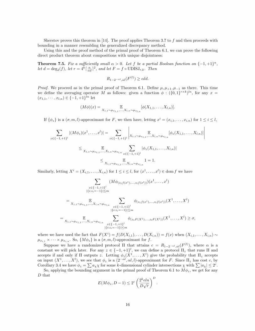
Sherstov proves this theorem in [14]. The proof applies Theorem 3.7 to f and then proceeds withbounding in a manner resembling the generalized discrepancy method.

Using this and the proof method of the primal proof of Theorem 6.1, we can prove the followingdirect product theorem about compositions with unique disjointness:

Theorem 7.5. Fix a sufficiently small α > 0. Let f be a partial Boolean function on −1,+1n,let d = degδ(f), let r = 4kd n Thenαde

2, and let F = f UDISJr,k.

R (l)1−2−αl,αl(F ) ≥ αld.

Proof. We proceed as in the primal proof of Theorem 6.1. Define µ, µ+1, µ−1 as there. This timewe define the averaging operator M as follows: given a function φ : (0, 1r×k)ln, for any x =(x ln

1,1, · · · , xl,n) ∈ −1,+1 let

(Mφ)(x) = E [φ(X1,1, . . . , Xl,n)].X1,1∼µx ,...,Xl,n∼µx1,1 l,n

If φz is a (σ,m, l)-approximant for F , we then have, letting xi = (xi,1, . . . , xi,n) for 1 ≤ i ≤ l,

∑|(Mφ . . , xlz)(x

1, . )| =∑ ∣∣∣∣∣ E [φz(X1,1, . . . , Xl,n)]

X1,1 µx ,...,Xl,n1,1z 1,+1 l z 1,+1 l

∼ ∼µx∈− ∈− l,n

∣∣∣∣≤ E φz(X1,1, . . . , Xl,n)

∣X1,1∼µx ,...,Xl,n∼µx1,1 l,n

|z

∑|

∈−1,+1l

≤ E 1 = 1.X1,1∼µx ,...,Xl,n µx1,1

∼l,n

Similarly, letting Xi = (Xi,1, . . . , X1 l

i,n) for 1 ≤ i ≤ l, for (x , . . . , x ) ∈ dom f we have∑(Mφ )(x1, . . . , xl(z x1),...,zlf(xl1f( )) )

z∈−1,+1l|i:zi=−1|≤m

= E φ(z f(x11 ),...,zlf(xl))(X

1, . . . , X l)X1,1∼µx ,...,Xl,n µx1,1

∼l,n

z∈−|i:zi=

∑1,+1l−1|≤m

= E∑

φ(z 1 l1F (X ),...,zlF (X ))(X

1, . . . , X l) σ,X1,1∼µx ,...,Xl,n µx1,1

∼l,n

z 1,+1l≥

∈−|i:zi=−1|≤m

where we have used the fact that F (Xi) = f(D(Xi,1), . . . , D(Xi,n)) = f(x) when (Xi,1, . . . , Xi,n) ∼µxi,1 × · · · × µxi,n . So, Mφz is a (σ,m, l)-approximant for f .

Suppose we have a randomized protocol Π that attains c = R (F (l)1−2−αl,αl ), where α is a

constant we will pick later. For any z ∈ −1,+1l, we can define a protocol Πz that runs Π andaccepts if and only if Π outputs z. Letting φz(X

1, . . . , X l) give the probability that Πz acceptson input (X1, . . . , X l), we s∑ee that φz is a (2−αl, αl, l)-approximant for F . Since Πz has cost c, byCorollary 3.4 we have φz = aχχ for some k-dimensional cylinder intersections χ with |aχ| ≤ 2c.

So, applying the bounding argument in the primal proof of Theorem 6.1 to Mφz, we

∑get for any

D thatn

E(Mφz, D − 1) 2c(

2kel≤D√r

)D.

16

Assume for the sake of contradiction that c < αld. Setting D = βld then gives

E(Mφz, D − 1) ≤ 2αld(

2keln

βld2kd n(

αd

)βld≤ 2αld αe/β)βld.

e

So there is a system of polynomials pz with degree less than βld satisfyingαld βld

‖Mφz − pz‖∞ ≤2 (αe/β) for each z. Taking α sufficiently small compared to β makes pz − 2αld(αe/β)βldsatisfy the necessary properties for a (2−βld, βl, l)-approximant for f . But deg(pz) < βld for all z,contradicting Theorem 7.4. So in fact we have c ≥ αld, as desired.

Theorem 7.2 follows as a corollary:

Proof of Theorem 7.2. This follows from Theorem 7.5 in the same way that Theorem 1.1 follows

from Theorem 6.1. Specifically, since deg1/3(ANDn) ≥ c√n for some c, letting f = ANDn and

d = c√n in Theorem 7.5 gives a bound equivalent to the result we want.

8 Relation to the Generalized Inner ProductgIn the introduction, we defined Gn,k as a function g on the bits where all players receive a 1. We

noted that DISJn,k = GNORn,k and that the generalized inner product GIPn,k = GPARITY

n,k . Both ofthese are derivatives on the number of shared 1-bits among all players, with GIP being the resultmod 2 and DISJ being whether the result is 0. Despite their similarities in form, it has been mucheasier to prove stronger bounds for GIP than DISJ.

In 1992, Babai, Nisan, and Szegedy [1] showed that R1/3(GIPn,k) = Ω( n4k

). This was soon shown

to be close to optimal, as the original proof by Grolmusz [7] in 1994 showed D(GIPn,k) = O(kn ).2k

As we showed in Section 2, that protocol can be extended to a O(k2n2k

) protocol for DISJ (or anyGgn,k where g depends only on the number of 1s).

Before [13], the best lower bounds for DISJ for k ≥ 3 players were weaker than Ω(( n 132k

) /(k+1))

and [13] improved this only to Ω(( n4k

)1/4). The best lower bound on randomized complexity currently

available is Ω(√nk ). Thus twenty years after [7] showed GIP is Θ(n) for constant k, we still have an

2 k

Ω(n1/2), O(n) gap for DISJ.Intuitively, this difference in difficulty in placing lower bounds comes from the fact that the value

of PARITY depends on all of its inputs while on all but the 0 input, NOR can depend on a singlebit. Informally, this makes PARITY harder to approximate.

In fact, Sherstov [13] in achieving the bound for DISJ uses the hardness of PARITY, as we sawin Section 4 in the definition of Γ = disc(

⊕UDISJ).

9 Discussion

It is natural to ask how far the methods used in proving lower bounds so far can take us. To break thelongstanding barrier and get the first Ω(nc/2O(k)) bound on the randomized complexity of DISJn,kfor a constant c, Sherstov [13] needed to modify the usual approach of applying the generalizeddiscrepancy method and the pattern matrix method, forming bounds on the individual terms of theFourier decomposition, and exploiting properties like conditional independence in the probabilitydistributions. To improve this bound to Ω(n1/2/2O(k)), Sherstov [15] again had to introduce newtechniques, this time including more analytic tools like directional derivatives.

It remains open whether R (DISJ ) ≥ Ω(n/2O(k)1/3 n,k ), and whether such a bound can be proven

using the kinds of approaches that have been used so far like using cylinder intersections, discrep-ancies, and polynomial approximations.

17

In addition, although essentially tight bounds have been proven for the deterministic and quan-tum communication complexity of UDISJn,k using adaptations of Sherstov’s methods in [13], thereare still many other protocol settings to consider for which the sharp bounds have not yet beendetermined. For example, nondeterministic and Merlin-Arthur protocols are two types that areaddressed in [13] and [15], but for which polynomial gaps between upper and lower bounds stillremain.

Finally, results like Theorem 6.1 allow us to generalize our lower bounds to compositions ofdisjointness with other functions f , assuming corresponding polynomial lower bounds on f . Infact, Sherstov [13] also shows that similar bounds on compositions hold with UDISJn,k replacedby different expressions like ORk ∨ ANDk. It is open to determine how much these results can begeneralized – how complicated the functions we compose with in place of UDISJn,k can get – whilestill allowing us to prove strong lower bounds on randomized communication complexity using anessentially similar method.

References

[1] Babai, L., Nisan, N., and Szegedy, M. Multiparty protocols, pseudorandom generators forlogspace, and time-space trade-offs. J. Comput. Syst. Sci. 45, 2 (Oct. 1992), 204–232.

[2] Beame, P., and Huynh-Ngoc, D.-T. Multiparty communication complexity and thresholdcircuit size of AC0. In Proceedings of the 2009 50th Annual IEEE Symposium on Foundations ofComputer Science (Washington, DC, USA, 2009), FOCS ’09, IEEE Computer Society, pp. 53–62.

[3] Beame, P., Pitassi, T., Segerlind, N., and Wigderson, A. A strong direct producttheorem for corruption and the multiparty communication complexity of disjointness. Comput.Complex. 15, 4 (Dec. 2006), 391–432.

[4] Chandra, A. K., Furst, M. L., and Lipton, R. J. Multi-party protocols. In Proceedings ofthe Fifteenth Annual ACM Symposium on Theory of Computing (New York, NY, USA, 1983),STOC ’83, ACM, pp. 94–99.

[5] Chattopadhyay, A., and Ada, A. Multiparty communication complexity of disjointness.CoRR (2008).

[6] Chor, B., and Goldreich, O. Unbiased bits from sources of weak randomness and proba-bilistic communication complexity. SIAM J. Comput. 17, 2 (Apr. 1988), 230–261.

[7] Grolmusz, V. The bns lower-bound for multiparty protocols is nearly optimal. Inf. Comput.112, 1 (July 1994), 51–54.

[8] Kalyanasundaram, B., and Schintger, G. The probabilistic communication complexityof set intersection. SIAM Journal on Discrete Mathematics 5, 4 (1992), 545–557.

[9] Klauck, H. A strong direct product theorem for disjointness. In Proceedings of the forty-secondACM symposium on Theory of computing (2010), ACM, pp. 77–86.

[10] Lee, T., and Shraibman, A. Disjointness is hard in the multi-party number on the foreheadmodel. CoRR (2007).

[11] Nisan, N., and Szegedy, M. On the degree of boolean functions as real polynomials. InProceedings of the Twenty-fourth Annual ACM Symposium on Theory of Computing (New York,NY, USA, 1992), STOC ’92, ACM, pp. 462–467.

18

[12] Sherstov, A. A. The pattern matrix method for lower bounds on quantum communication.In Proceedings of the Fortieth Annual ACM Symposium on Theory of Computing (New York,NY, USA, 2008), STOC ’08, ACM, pp. 85–94.

[13] Sherstov, A. A. The multiparty communication complexity of set disjointness. In Proceedingsof the Forty-fourth Annual ACM Symposium on Theory of Computing (New York, NY, USA,2012), STOC ’12, ACM, pp. 525–548.

[14] Sherstov, A. A. Strong direct product theorems for quantum communication and querycomplexity. SIAM Journal on Computing 41, 5 (2012), 1122–1165.

[15] Sherstov, A. A. Communication lower bounds using directional derivatives. Journal of theACM (JACM) 61, 6 (2014), 34.

[16] Tesson, P. Computational Complexity Questions Related to Finite Monoids and Semigroups.PhD thesis, Montreal, Que., Canada, Canada, 2003.

19

MIT OpenCourseWarehttps://ocw.mit.edu

18.405J / 6.841J Advanced Complexity TheorySpring 2016

For information about citing these materials or our Terms of Use, visit: https://ocw.mit.edu/terms.