nonlocality & communication complexity

Nonlocality &Communication Complexity

Wim van DamWolfson College

Centre for Quantum ComputationDepartment of Physics, University of Oxford

Thesis submitted for the degree of Doctor of Philosophy in Physics at the Faculty ofPhysical Sciences, University of Oxford.

Nonlocality & Communication Complexity

Wim van DamWolfson College, University of Oxford

D.Phil. thesis, Department of PhysicsMichaelmas Term 1999

Abstract

This thesis discusses the connection between the nonlocal behavior of quantum me-chanics and the communication complexity of distributed computations. The first threechapters provide an introduction to quantum information theory with an emphasis onthe description of entangled systems. The next chapter looks at how to measure thecomplexity of distributed computations. This is expressedby the ‘communication com-plexity’, defined as the minimum amount of communication required for the evaluationof a function

� ��—a communication necessary because the input strings� and�are distributed over separated parties. In the theory of quantum communication, we tryto use the nonlocal effects of entangled quantum bits to reduce communication com-plexity. In chapters 5, 6 and 7, such an improvement over classical communication isindeed established for various functions. However, it is also shown that entanglementdoes not lead to a more efficient calculation of the inner product function. We thusreach the conclusion that nonlocality sometimes—but not always—allows a reductionin communication complexity. This subtle relationship between nonlocality and com-munication vanishes when we consider ‘superstrong’ correlations. We demonstrate thatif a violation of the Clauser-Horne-Shimony-Holt inequality with the maximum factorof � is assumed, all decision problems have the same trivial complexity of a single bit.The thesis concludes with an overview of the current status of quantum communicationtheory, and a discussion of the experimental feasability ofthe suggested protocols.

Acknowledgements

I would like to thank Artur Ekert for his guidance during my D.Phil. period at the Cen-tre for Quantum Computation. (I know that he does not like to be called a ‘supervisor’of anything or anybody, so I will refrain from doing so.) He created the freedom forme to do what I thought was best, while giving me ample opportunities to make themost out of my Oxford years. His view—that doing science is a joint effort that shouldbe fun—was refreshing during my first encounters with the academic profession. Andfun it was.

Many people helped me during my scientific explorations. I feel privileged to thankthe following researchers for both their insightful comments and the enjoyable discus-sions I had with them: Andris Ambainis, P.K. Aravind, Guido Bacciagaluppi, SimonBenjamin, Andre Berthiaume, Dik Bouwmeester, Dagmar Bruß, Harvey Brown, HarryBuhrman, Richard Cleve, Mauro D’Ariano, David Deutsch, Mark Ettinger, LanceFortnow, Michael Freedman, Chris Fuchs, Daniel Gottesman,Frederic Green, Pe-ter Grunwald, Rasmus Hvas Hansen, Lucien Hardy, Patrick Hayden, Leah Hender-son, Alexander Holevo, Peter Høyer, Neil Johnson, JonathanJones, Richard Jozsa,Adrian Kent, Sophie Laplante, Helger Lipmaa, Hoi-Kwong Lo,Chiara Macchiavello,Frederic Magniez, David Meyer, Mike Mosca, Ashwin Nayak,Michael Nielsen, AsherPeres, Martin Plenio, Sandu Popescu, John Preskill, John Rogers, Louis Salvail, MiklosSantha, Ben Schumacher, Jason Semitecolos, Sjoerd Stallinga, Andrew Steane, AlainTapp, Barbara Terhal, John Tromp, Umesh Vazirani, Vlatko Vedral, Paul Vitanyi, JohnWatrous, Harald Weinfurter, Reinhard Werner, Ronald de Wolf, and Anton Zeilinger.

This research would not have been possible without the financial support of theInstitute for Logic, Language and Computation in Amsterdam, and the European TMRResearch Network (ERP-4061PL95-1412). I also enjoyed the contributions and hos-pitality of a great many other groups and institutions. Theyenabled me to do an al-most obscene amount of travelling while I was supposed to be working on this thesis,and I want to thank them for this. They are: Berkeley, BRICS Aarhus, CIDEC Es-tonia, CWI Amsterdam, Elsag-Bailey, Hewlett Packard Bristol, Imperial College, ISITorino, LRI Orsay, Microsoft Redmond, the Novartis Foundation, NWO, UNISYS, theTMR-Network of the European Commission, Wolfson College, and the universities ofBielefeld, Delft, Helsinki, Milan, Pavia and Utrecht.

Finally, my parents and friends are thanked for their love, understanding and friend-ship. All of the above should realize however, that they are only ‘second place’, as mygreatest gratitude goes to my dearest Heather. Besides her encouragement, trust andrigorous proofreading, I thank her for our love.

page 3

Preface

This is the D.Phil. thesis of Wim van Dam. It contains the workthat I did as a graduatestudent under the supervision of Artur Ekert at the Centre for Quantum Computation,University of Oxford.

The main part of this thesis deals with the investigation of quantum communicationprotocols that have a smaller complexity than any possible classical protocol: that is,quantum communication complexity. This advantage of quantum over classical is madepossible by the nonlocal correlations, which can be established with entangled quantumbits.

The first four chapters of this thesis are of an introductory nature. In them, I givea brief overview of, respectively, quantum information, quantum communication, non-locality, and communication complexity theory. Chapter 5 gives an example of twoquantum communication protocols that have a reduced complexity when compared toclassical procedures. The results of this chapter are described in

� “Quantum entanglement and communication complexity”, by Harry Buhrman,Richard Cleve, and Wim van Dam, Technical Report RS-97-40 inthe BRICSResearch Series, University of Aarhus; quant-ph archive, report no. 9705033,

where the phrasing of the quantum protocol is due to the author of this thesis.The 6th chapter generalizes the above protocol to the multiparty setting. It was

published earlier as a part of

� “Multiparty quantum communication complexity”, by Harry Buhrman, Wimvan Dam, Peter Høyer, and Alain Tapp,Physical Review A, Volume 60, No. 4,pp. 2737–2741 (1999); quant-ph archive, report no. 9710054.

The proof method of the classical lower bound is my main contribution to this article.Together with Lucien Hardy, I published the paper that is described in Chapter 7,

� “Quantum communication using a nonlocal Zeno effect”, Lucien Hardy andWim van Dam,Physical Review A, Volume 59, No. 4, pages 2635–2640 (1999);quant-ph archive, report no. 9805037.

It shows how the quantum Zeno effect of an entangled pair of qubits can be used toreduce the error in a one-bit communication protocol. The derivation of the minimalclassical error rate is by my hand.

page 4

Chapter 8 shows that there are distributed functions that donot allow a reductionin complexity by the use of entanglement. The analysis of thetwo-bit case is mycontribution to this part, with the corresponding publication

� “Quantum entanglement and the communication complexity ofthe inner prod-uct function”, by Richard Cleve, Wim van Dam, Michael Nielsen, and AlainTapp,Proceedings of the 1st NASA International Conference on Quantum Com-puting and Quantum Communications, in Lecture Notes in Computer Science,No. 1509, (editor: Colin P. Williams), Springer-Verlag, pages 61–74 (1999);quant-ph archive, report no. 9708019.

The last chapter before the Conclusion discusses the consequences of superstrongnonlocality for communication complexity. This work will be published in the nearfuture as a single author article.

page 5

Contents

1 Introducing Quantum Information and Communication 91.1 Modeling Information . . . . . . . . . . . . . . . . . . . . . . . . . . 91.2 Quantum Information . . . . . . . . . . . . . . . . . . . . . . . . . . 101.3 Time Evolution of Quantum Bits . . . . . . . . . . . . . . . . . . . . 111.4 Measurements . . . . . . . . . . . . . . . . . . . . . . . . . . . . . . 111.5 Limitations of Dirac’s Ket Notation . . . . . . . . . . . . . . . . .. 121.6 Density Matrices . . . . . . . . . . . . . . . . . . . . . . . . . . . . 121.7 Separated Systems . . . . . . . . . . . . . . . . . . . . . . . . . . . 141.8 Von Neumann Entropy of Mixed States . . . . . . . . . . . . . . . . 151.9 Operations on Mixed States . . . . . . . . . . . . . . . . . . . . . . . 151.10 Operator Sum Representation . . . . . . . . . . . . . . . . . . . . . .161.11 A Few Elementary Operations . . . . . . . . . . . . . . . . . . . . . 181.12 No Influence-at-a-Distance . . . . . . . . . . . . . . . . . . . . . . .19

2 Quantum Communication 212.1 Entanglement . . . . . . . . . . . . . . . . . . . . . . . . . . . . . . 212.2 An Example: Werner States . . . . . . . . . . . . . . . . . . . . . . . 222.3 Superdense Coding . . . . . . . . . . . . . . . . . . . . . . . . . . . 232.4 Teleportation . . . . . . . . . . . . . . . . . . . . . . . . . . . . . . 242.5 Information versus Information Representation . . . . . .. . . . . . 252.6 Holevo’s Bound and an Appendix to It . . . . . . . . . . . . . . . . . 262.7 Optimality of Superdense Coding and Teleportation . . . .. . . . . . 26

3 Nonlocality 283.1 Bell’s Inequality . . . . . . . . . . . . . . . . . . . . . . . . . . . . . 283.2 Classical or Hidden Variables Models . . . . . . . . . . . . . . . .. 283.3 Two-Party Nonlocality . . . . . . . . . . . . . . . . . . . . . . . . . 303.4 Three-Party Nonlocality . . . . . . . . . . . . . . . . . . . . . . . . 313.5 Locality Loopholes . . . . . . . . . . . . . . . . . . . . . . . . . . . 32

4 Communication Complexity 344.1 Introduction . . . . . . . . . . . . . . . . . . . . . . . . . . . . . . . 344.2 Two-Party Communication Complexity . . . . . . . . . . . . . . . .344.3 Some Observations about Communication Complexity . . . .. . . . 35

page 6

CONTENTS

4.4 Formal Definition of Deterministic Communication . . . . .. . . . . 354.5 Probabilistic Protocols . . . . . . . . . . . . . . . . . . . . . . . . . 384.6 An Application of Von Neumann’s Min-Max Theorem . . . . . . .. 404.7 Proving Probabilistic Bounds . . . . . . . . . . . . . . . . . . . . . .424.8 Relations and Problems with a Promise . . . . . . . . . . . . . . . .434.9 Quantum Communication with Entanglement . . . . . . . . . . . .. 434.10 Other Quantum Communication Models . . . . . . . . . . . . . . . .444.11 Multiparty Communication Complexity . . . . . . . . . . . . . .. . 454.12 Assumptions throughout this Thesis . . . . . . . . . . . . . . . .. . 464.13 History and References . . . . . . . . . . . . . . . . . . . . . . . . . 47

5 Two Simple Quantum Communication Protocols 485.1 Reducing Errors with Nonlocality . . . . . . . . . . . . . . . . . . .485.2 Limitations of Classical Protocols . . . . . . . . . . . . . . . . .. . 495.3 An Exact Three-Party Quantum Protocol . . . . . . . . . . . . . . .. 505.4 Impossibility of a Two Bit Classical Protocol . . . . . . . . .. . . . 51

6 Multiparty Quantum Communication Complexity 536.1 Multiparty Problem and Its Quantum Complexity . . . . . . . .. . . 536.2 The Quantum Protocol . . . . . . . . . . . . . . . . . . . . . . . . . 536.3 Bounds for Promise Functions . . . . . . . . . . . . . . . . . . . . . 546.4 The Lower Bound for the Classical Protocol . . . . . . . . . . . .. . 556.5 Conclusion . . . . . . . . . . . . . . . . . . . . . . . . . . . . . . . 57

7 Quantum Whispers 587.1 Introduction . . . . . . . . . . . . . . . . . . . . . . . . . . . . . . . 587.2 The Two-Party Problem . . . . . . . . . . . . . . . . . . . . . . . . . 587.3 The Quantum Protocol . . . . . . . . . . . . . . . . . . . . . . . . . 597.4 Best Possible Classical Protocol . . . . . . . . . . . . . . . . . . .. 617.5 Multiparty Communication Problem . . . . . . . . . . . . . . . . . .637.6 The Quantum Whispers Protocol . . . . . . . . . . . . . . . . . . . . 637.7 Error of the Quantum Whispers Protocol . . . . . . . . . . . . . . .. 647.8 Possible Classical Whispers . . . . . . . . . . . . . . . . . . . . . . 64

8 Lower Bounds for Quantum Communication 668.1 Introduction . . . . . . . . . . . . . . . . . . . . . . . . . . . . . . . 668.2 The Inner Product Problem . . . . . . . . . . . . . . . . . . . . . . . 678.3 Informal Sketch of Proof . . . . . . . . . . . . . . . . . . . . . . . . 688.4 Quantum Parallelizing Communication Protocols . . . . . .. . . . . 688.5 Bounds on Exact Inner Product Protocols . . . . . . . . . . . . . .. 698.6 Bounds on Probabilistic Inner Product Protocols . . . . . .. . . . . . 708.7 Communication with Classical Bits . . . . . . . . . . . . . . . . . .. 718.8 Inner Product Problem for Two Bits . . . . . . . . . . . . . . . . . . 728.9 The Classical Case for Two Bits . . . . . . . . . . . . . . . . . . . . 728.10 The Quantum Improvement . . . . . . . . . . . . . . . . . . . . . . . 748.11 Communication Complexity versus Quantum Mechanics . .. . . . . 74

page 7

CONTENTS

9 Superstrong Correlations versus Communication Complexity 769.1 Nonlocality Revisited . . . . . . . . . . . . . . . . . . . . . . . . . . 769.2 The Question of Popescu and Rohrlich . . . . . . . . . . . . . . . . .779.3 Distributed Decision Problems as Inner Products . . . . . .. . . . . 789.4 Inner Product and Nonlocality . . . . . . . . . . . . . . . . . . . . . 799.5 Trivial Superstrong Communication Complexity . . . . . . .. . . . . 809.6 Discussion . . . . . . . . . . . . . . . . . . . . . . . . . . . . . . . . 81

10 Conclusion 8210.1 Other Work on Quantum Communication . . . . . . . . . . . . . . . 8210.2 Open Problems and Future Research . . . . . . . . . . . . . . . . . .8310.3 Thresholds for Experimental Implementations . . . . . . .. . . . . . 8410.4 Thresholds for a One Bit Protocol . . . . . . . . . . . . . . . . . . .8510.5 Noisy Entangled States . . . . . . . . . . . . . . . . . . . . . . . . . 8510.6 Inexact Measurement Devices . . . . . . . . . . . . . . . . . . . . . 8510.7 Conclusion . . . . . . . . . . . . . . . . . . . . . . . . . . . . . . . 86

A Appendix to Holevo’s Bound 87A.1 Information Transfer with Quantum States . . . . . . . . . . . .. . . 87A.2 Holevo’s Bound versus Superdense Coding . . . . . . . . . . . . .. 88A.3 Holevo’s Bound in the Presence of Entanglement . . . . . . . .. . . 88

page 8

Chapter 1

Introducing QuantumInformation andCommunication

In this thesis we investigate the theory of quantum information and communication.The current interest in this field is fueled by the discovery that the use of quantummechanical processes provides us with an advantage over thetraditional, classical waysof manipulating information. In this chapter I will introduce the notion of ‘quantuminformation’, and the standard notation as it will be used throughout the rest of thethesis.

Section 1.1 Modeling Information

The term ‘bit’ stands for ‘binary digit’, which reflects the fact that it can be describedand implemented by a two-level system. Conventionally, these two levels are indicatedby the labels “zero” and “one”, or “

�” and “�”. If we want to capture more than two

possibilities, more bits are needed: with� bits we have�� different labels.The abstraction from� two-level systems to the set�� of size�� takes us away

from the physical details of the implementation of a piece ofmemory in a computer,and instead focuses on a more mathematical description of information. This ‘physicsindependent’ approach to standard information theory has been extremely successfulin the past decades: it enables a general understanding of computational and commu-nicational processes that is applicable to all the different ways of implementing theseprocesses. It is for this reason that the Turing machine model of computation gives anaccurate description of both the mechanical computer suggested by Charles Babbageand the latest Silicon based Pentium III processors, despite their obvious physical dif-ferences. This does not mean that Turing’s model ignores thephysical reality of build-ing a computer, on the contrary. The observation that it would be unphysical to assumean infinite or unbounded precision in the components of a computer is expressed by

page 9

1.2. QUANTUM INFORMATION

Turing’s rule that per time-step only a fixed, finite amount ofcomputational work canbe done.[63] The proper analysis of algorithms in the theoryof computational com-plexity relies critically on the exclusion of computational models that are not realistic.Such models often give the wrong impression that certain complicated tasks are easy.(A good example of this is the result that the factorization of integers can be done inpolynomial time if we assume that addition, multiplicationand division of arbitrarybig numbers can be done in constant time. (See Chapter 4.5.4,Exercise 40 in [40] and[60].) There is, however, also a danger with this axiomatization of the physical as-sumptions in information theory: believing that the assumptions are true. This is whathappened with the traditional view on information, forgotten were the implicit clas-sical assumptions that ignore the possibilities of quantummechanics. The realizationthat quantum physics describes a world where information behaves differently than inclassical theory led to the blossoming of several fields—quantum information, quan-tum computing, quantum communication, et cetera. In this thesis I will focus on thedifferences in communication complexity between a classical and a quantum model ofcommunication. Before doing so, it is necessary to define what we mean by quantuminformation and communication.

Section 1.2 Quantum Information

At the heart of quantum mechanical information theory lies thesuperposition principle.Where a classical bit is either in the state “zero” or “one”, aquantum bit is allowed tobe in a superposition of the two states. A qubit with the label� is therefore describedin Dirac’s bra-ket notation by the linear combination:

�� “zero”� � � �“one”��where for the complex valued amplitudes�, � � � , the normalization restriction

�� applies. In this formalism, the state space of a single qubitis built up bythe unit vectors in the two-dimensional Hilbert space. For � qubits, there are��basis states and hence the corresponding superposition is alinear combination of all��possible strings of� bits:

��

Again it is required that the amplitudes�� obey the normalization condition�� . (In Section 1.4 we will see the reason behind this stipulation.) The state space of� qubits is the�-fold tensor product of the state space of a single qubit. This space isidentical with a single��-dimensional Hilbert space:

�� For our purposes we will only use finite sets of quantum bits, so there is no need tolook at infinite-dimensional Hilbert spaces.

page 10

1.3. TIME EVOLUTION OF QUANTUM BITS

Section 1.3 Time Evolution of Quantum Bits

Quantum mechanics only allows transformations of states that are linear and respectthe normalization restriction. When acting on an�-dimensional Hilbert space, theseare the� �� complex valued rotation matrices that are norm preserving:the unitarymatrices of U

��. It is easy to show that this corresponds exactly to the requirement thatthe inverse of

�is the complex conjugate

��of the matrix. (The complex conjugate

is defined by�� , where�

‘row’ � ‘column’�

is used to denote thedifferent matrix entries.)

The effect of a unitary transformation�

on a state� is exactly described by the cor-responding rotation of the vector

�� in the appropriate Hilbert space. For this reason,“�

” stands both for the quantum mechanical transformation as well as for the unitaryrotation:

� ��

� � �� It follows from the associativity of matrix multiplicationthat the effect of two consec-utive transformation

�� and� is the same as the single transformation

�� . Justas matrix multiplication does not commute, so does the orderof a sequence of unitarytransformations matter: in general

�� . We can restate this in a more intu-itive way by saying that it makes a difference if we first do

�� and then�, or the other

way around. (A convincing example is that of the two actions “add five” and “multiplyby two”.)

Section 1.4 Measurements

When measuring the state�� , the probability of observing the outcome

“�” equals

�� . This explains the normalization restriction on the amplitudes: thedifferent probabilities have to add up to one. But what exactly is a ‘measurement’ andan ‘observation’, and how do we describe this mathematically? These are thorny issuesthat this thesis will leave untouched. Here we will only givea formal description of themeasurement process and a short explanation of why this is such a problematic part ofquantum mechanics.

The possible outcomes “�” of � correspond to a set of orthogonal vectors��

of the measuring device. This device can be our own eye or somekind of machine,but the crucial point is that ‘measuring�’ implies ‘interacting with�’. The effect on�of such a measurement is that the statecollapsesaccording to the outcome “

�” of our

observation. This is described by the transformation:

� �� (1.1)

The collapse as described above is a non-unitary transformation. This is typical whenwe try to describe the behavior of� as it interacts with a system that lies outside of the

page 11

1.5. LIMITATIONS OF DIRAC’S KET NOTATION

state. (We say that� is an ‘open system’.) When we view� and the measurement de-vice togetherduring the observation, the evolution becomes unitary again. Our currentexample is then described by the transformation:

� �� measurement device� �

� � �� outcome��The problem with this last description is that it no longer specifies the specific outcome“�” that we seem to observe. It is here where the debate on themeasurement problem

starts and our discussion ends.For the purposes of this thesis it is more convenient to use the terminology of the

collapsing quantum state. We will therefore describe the effect of a measurement as inEquation 1.1 for practical reasons. (This does not imply that I really think that there issuch a collapse, but this issue are not the topic of this text.In this thesis we are mainlyinterested in the differences between the classical and thequantum mechanical theoryof information. These differences, expressed in probabilities et cetera, are independentof the viewpoint that one has on the measurement problem.)

We just described the traditional ‘Von Neumann measurement’ where we observethe state� in the canonical basis spanned by the basis vectors

�. Other, more subtle,

measurement procedures are also possible by choosing an in-or over-complete basis.We will postpone the description of these two options the point when we discuss thedensity matrix formalism, which is more suitable for the general theory of interactingquantum mechanical systems.

Section 1.5 Limitations of Dirac’s Ket Notation

The braket notation that we discussed above is tailor-made for the description of closedquantum mechanical systems. By this we mean the evolution ofstates that do notinteract with an exterior environment. When we also want to consider the behavior ofopen systems, the ket-notation becomes less suitable. Thiswas already obvious in thediscussion of the measurement procedure where we had to expand the set of unitaryoperations with a probabilistic procedure that ‘collapses’ the quantum state to one ofthe basis states. One cannot help but feel uncomfortable about this sudden change ofrules: is it not possible to deal with open and closed quantumsystems in the same way?Luckily, we find in the formalism of density matrices a positive answer to this question.

Section 1.6 Density Matrices

An �-dimensional pure state� can be expressed as a normalized vector�� in the

Hilbert space�. The complex conjugate�� of this vector is the bra

�� , which isan element of the adjoint space�

�. By taking the direct product between the ket��

and the bra�� , we thus obtain an� �� complex valued, Hermitian matrix: thedensity

matrix of �.

page 12

1.6. DENSITY MATRICES

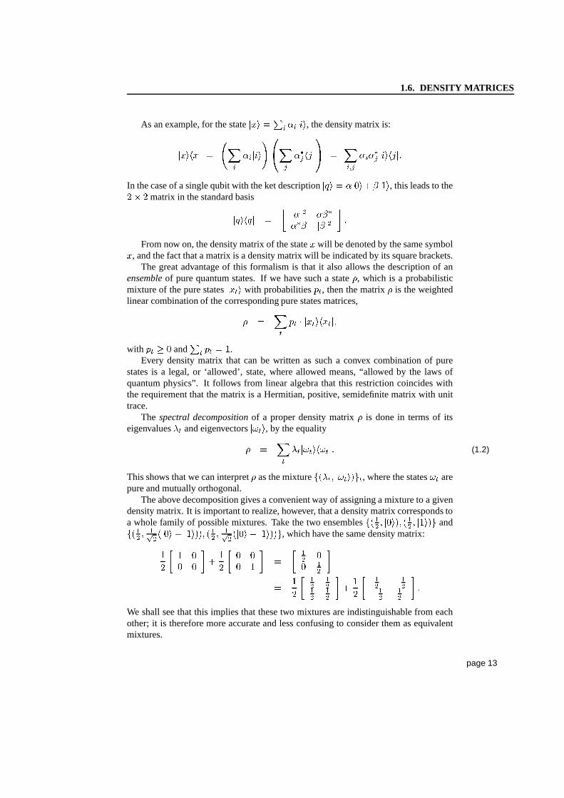
As an example, for the state�� , the density matrix is:

��

In the case of a single qubit with the ket description�� , this leads to the

� ��matrix in the standard basis

�� From now on, the density matrix of the state� will be denoted by the same symbol�, and the fact that a matrix is a density matrix will be indicated by its square brackets.The great advantage of this formalism is that it also allows the description of an

ensembleof pure quantum states. If we have such a state�, which is a probabilisticmixture of the pure states

�� with probabilities��, then the matrix� is the weightedlinear combination of the corresponding pure states matrices,

� � � �� with ��

and�� .Every density matrix that can be written as such a convex combination of pure

states is a legal, or ‘allowed’, state, where allowed means,“allowed by the laws ofquantum physics”. It follows from linear algebra that this restriction coincides withthe requirement that the matrix is a Hermitian, positive, semidefinite matrix with unittrace.

The spectral decompositionof a proper density matrix� is done in terms of itseigenvalues� and eigenvectors

��, by the equality

� � � � �� (1.2)

This shows that we can interpret� as the mixture�� , where the states�� arepure and mutually orthogonal.

The above decomposition gives a convenient way of assigninga mixture to a givendensity matrix. It is important to realize, however, that a density matrix corresponds toa whole family of possible mixtures. Take the two ensembles�� and�� , which have the same density matrix:

��

� � � � ��

� � � � � � ��

� ��

� � � ��

��

We shall see that this implies that these two mixtures are indistinguishable from eachother; it is therefore more accurate and less confusing to consider them as equivalentmixtures.

page 13

1.7. SEPARATED SYSTEMS

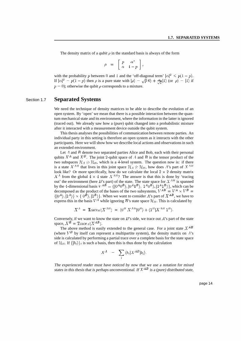
The density matrix of aqubit � in the standard basis is always of the form

� � � � ��

with the probability� between�

and � and the ‘off-diagonal term’�� .

If�� then� is a pure state with

�� (or�� if� � �

); otherwise the qubit� corresponds to a mixture.

Section 1.7 Separated Systems

We need the technique of density matrices to be able to describe the evolution of anopen system. By ‘open’ we mean that there is a possible interaction between the quan-tum mechanical state and its environment, where the information in the latter is ignored(traced out). We already saw how a (pure) qubit changed into aprobabilistic mixtureafter it interacted with a measurement device outside the qubit system.

This thesis analyses the possibilities of communication between remote parties. Anindividual party in this setting is therefore an open systemas it interacts with the otherparticipants. Here we will show how we describe local actions and observations in suchan extended environment.

Let � and� denote two separated parties Alice and Bob, each with their personalqubits�� and��. The joint �-qubit space of� and� is the tensor product of thetwo subspaces� ��, which is a�-level system. The question now is: if thereis a state�� that lives in this joint space� ��, how does�’s part of��look like? Or more specifically, how do we calculate the local� � � density matrix�� from the global� � � state��? The answer is that this is done by ‘tracingout’ the environment (here�’s part) of the state. The state space for�� is spannedby the�-dimensional basis �� , which can bedecomposed as the product of the bases of the two subsystems, �� . When we want to consider�’s part of��, we have toexpress this in the basis � while ignoring�’s state space�. This is calculated by

��

Conversely, if we want to know the state on�’s side, we trace out�’s part of the statespace,��

��.The above method is easily extended to the general case. For ajoint state��

(where � by itself can represent a multipartite system), the densitymatrix on�’sside is calculated by performing a partial trace over a complete basis for the state spaceof �. If �� is such a basis, then this is thus done by the calculation

��

The experienced reader must have noticed by now that we use a notation for mixedstates in this thesis that is perhaps unconventional. If�� is a (pure) distributed state,

page 14

1.8. VON NEUMANN ENTROPY OF MIXED STATES

then�� will refer to the (mixed) subsystem on�’s side. This means that we allowthe symbols�, � and even� to refer to a mixed state. I realize that this is not inaccordance with most of the literature, but it gives us a morenatural way of denotingthe different parts of a distributed system.

Section 1.8 Von Neumann Entropy of Mixed States

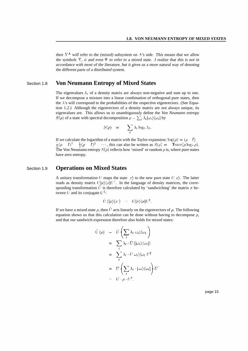
The eigenvalues� of a density matrix are always non-negative and sum up to one.If we decompose a mixture into a linear combination of orthogonal pure states, thenthe’s will correspond to the probabilities of the respective eigenvectors. (See Equa-tion 1.2.) Although the eigenvectors of a density matrix arenot always unique, itseigenvalues are. This allows us to unambiguously define theVon Neumann entropy�� of a state with spectral decomposition� � �� by

�� If we calculate the logarithm of a matrix with the Taylor expansion:�� , this can also be written as

�� .The Von Neumann entropy

�� reflects how ‘mixed’ or random� is, where pure stateshave zero entropy.

Section 1.9 Operations on Mixed States

A unitary transformation�

maps the state�� to the new pure state

� ��. The latterreads as density matrix

� �� . In the language of density matrices, the corre-sponding transformation�� is therefore calculated by ‘sandwiching’ the matrix� be-tween

�and its conjugate

��:

�� If we have a mixed state�, then �� acts linearly on the eigenvectors of�. The followingequation shows us that this calculation can be done without having to decompose�,and that our sandwich expression therefore also holds for mixed states:

��

page 15

1.10. OPERATOR SUM REPRESENTATION

It is clear that the positive eigenvalues� of � remain unchanged, and that�� onlyrotates the eigenvectors�� to the new eigenstates�� .

Unitary operations are an example of completely-positive,trace preserving maps:every positive, semidefinite matrix is mapped to (another) positive, semidefinite matrix,and the trace of the matrix remains unaltered. Complete-positivity, in combination withthe preservation of the trace, assures us that the result of atransformation will be aproper state if we started with a proper one.

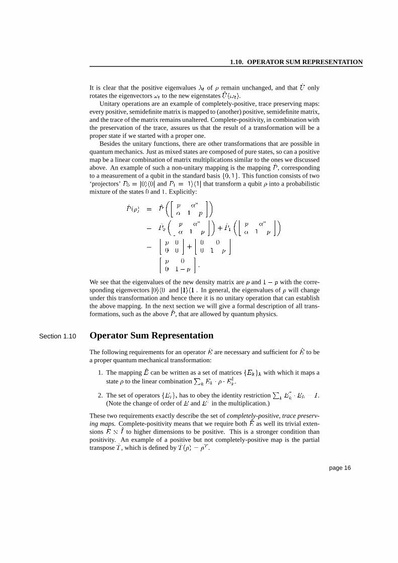
Besides the unitary functions, there are other transformations that are possible inquantum mechanics. Just as mixed states are composed of purestates, so can a positivemap be a linear combination of matrix multiplications similar to the ones we discussedabove. An example of such a non-unitary mapping is the mapping �� , correspondingto a measurement of a qubit in the standard basis�� . This function consists of two‘projectors’

�� and�� that transform a qubit� into a probabilistic

mixture of the states�

and�. Explicitly:

��

� � � � � � ��

� � � ��

We see that the eigenvalues of the new density matrix are� and� �� with the corre-sponding eigenvectors

�� and��. In general, the eigenvalues of� will change

under this transformation and hence there it is no unitary operation that can establishthe above mapping. In the next section we will give a formal description of all trans-formations, such as the above�� , that are allowed by quantum physics.

Section 1.10 Operator Sum Representation

The following requirements for an operator�� are necessary and sufficient for�� to bea proper quantum mechanical transformation:

1. The mapping�� can be written as a set of matrices�� with which it maps astate� to the linear combination��

�� .

2. The set of operators�� has to obey the identity restriction�� .

(Note the change of order of�

and��

in the multiplication.)

These two requirements exactly describe the set ofcompletely-positive, trace preserv-ing maps.Complete-positivity means that we require both�� as well its trivial exten-sions �� to higher dimensions to be positive. This is a stronger condition thanpositivity. An example of a positive but not completely-positive map is the partialtranspose�� , which is defined by�� .

page 16

1.10. OPERATOR SUM REPRESENTATION

We have truly extended the set of unitary transformations and measurements by theabove ‘operator sum’ formalism. An example of this is the mapping that erases a qubitand replaces it with the value zero. This non-unitary function is the combination of twooperators

��

and has the same effect on every qubit�, namely

��

� � � � � ��

� � ��

� � � ��

� � ��

We previously argued that a measurement has a non-unitary effect on a state be-cause we ignored its interaction with an outside system (themeasurement device). Thislesson holds for all allowed transformations:

Every completely-positive, trace preserving transformation �� of a system� can be viewed as a part of unitary mapping�� on a bigger system� ��. That �� by itself appears to be non-unitary is due to the factthat we ignore the space�.

It can be shown that for the extension of the system it is sufficient to assume that thedimension of the appended space� is twice as large as that of�, and that its initialstate is

�� . Hence, for every allowed quantum mechanical transformation �� thatacts on an�-dimensional system, there exists a unitary matrix

�� U�� such that

�� for all �. This is, in more general terms, the difference that we encountered betweenthe Equations 1.1 and 1.2. The non-unitary ‘collapse’ associated with an observation,or any other kind of interaction, is again a unitary transformation when we incorporatethe measurement device into the description of the event.

The converse of the earlier statement also holds: every mapping that can be writ-ten as a traced-out, unitary transformation on a larger Hilbert space is a completely-positive, trace preserving mapping. The reader is referredto the standard book byAsher Peres[53] and the article by Benjamin Schumacher[59]for a more extended andrigorous treatment of this ‘operator sum representation’.

page 17

1.11. A FEW ELEMENTARY OPERATIONS

Section 1.11 A Few Elementary Operations

In quantum computing and communication we look at the possibilities of transforminginformation as is allowed by the laws of quantum mechanics. We usually decomposesuch quantum algorithms in a series of small elementary steps that consist of one andtwo qubit operations. The following unitary gates are so commonly used that we willdefine them here in the introduction; we can therefore then use them throughout therest of the thesis without having to specify them.

The Not gate: This is the same gate that we know of in classical computationwith theadditional characteristic that it respects the superposition of a qubit:

NOT��

Phase Flip: The FLIP gate changes the phase of a qubit conditional on its value:

FLIP��

Phase Rotation: A more general phase rotation is provided by the PHASE operationwhich has a free variable� that determines the angle of the phase change:

PHASE��

(Note: FLIP � PHASE��.)

Hadamard transform: This transformation� maps the zero and one state to a super-position of the two basis states:

� �� and � �� The Hadamard is its own inverse (�

� �) and is often used in parallel on a� qubit register. Such a�-fold application of� translates the information of aclassical string into the phases of a full superposition andback again:��

��

��

where�� is the inner product modulo� of the� bit vectors� and�.

Rotations: With the rotation with an angle�, we mean the unitary one qubit trans-formation:

�� Controlled-Flip: The controlled-flip is a two-qubit operation that applies the FLIP

gate to the target bit, if the control bit equals “�”; otherwise it leaves the targetunchanged:

CFLIP��

�� for all �� .

page 18

1.12. NO INFLUENCE-AT-A-DISTANCE

Section 1.12 No Influence-at-a-Distance

We conclude this chapter by a brief look at the typical example of a two qubit entangledstate. Let�� be the pure state

�� . As a density matrix, thisreads in the standard basis:

��

� � � ��

��

When ‘viewed’ from either side as a subsystem, this pure state equals the maximallymixed qubit:

��

The complete, entangled state is therefore fundamentally different from the tensorproducts of its subsystems:�� . In the next chapters we will see howdifferent these entangled states are from states that can bewritten as tensor products.But before doing that, we will finish our introduction with anexplanation why entan-glementcannotbe used for instantaneous information transfer.

Entanglement between Alice and Bob does not allow Bob to indirectly influencethe state of Alice’s system. Let�� be the joint state (and hence�� the systemAlice’s side). Everything that Bob can do with his part��, can be described with theoperator-sum representation. That this does not effect Alice’s system can be expressedby the following equations. In the most general setting, thesystem�� is a mix-ture of pure states

�� , where each state can be written as a bipartite superposition�� . This gives the following summation with probabilities��,and amplitudes��:

��

� � ��

From this expression we can now calculate the density matrixof Alice’s subsystem�� with the partial trace over Bob’s part. This shows us that�� is independent ofthe local transformations that Bob may have applied to his part ��. For, if we assumethat this action has the operator sum representation��

�� , then the

page 19

1.12. NO INFLUENCE-AT-A-DISTANCE

‘new’ state �� on Alice’s side equals��

� ��

�

��

� �� (The last step in the above derivation uses the fact that�� in combination with the restriction that��

�� .) Clearly, the final outcome�� does not depend on the remote operation�� of Bob, and hence equals the original

state��.

page 20

Chapter 2

Quantum Communication

The theory of quantum communication looks at the consequences for informationtransfer if we allow the settings where we can send qubits anduse entanglement. Inthis chapter some of the possibilities and impossibilitiesof quantum communicationare explored. We pay special attention to the procedure of teleporting quantum stateswith classical signals. Also Holevo’s bound on the amount ofinformation that can betransfered with quantum signals is discussed.

Section 2.1 Entanglement

At the end of the previous chapter, we encountered a combination of two entangledqubits distributed over two parties� and�:

�� . It is impossibleto write this pure state as a tensor product� � �

. Even if we allow a mixture of tensorproducts, such a decomposition remains impossible. We say that the �� is anentangled state.More explicitly, the definition of entanglement is as follows:

A bipartite system�� is separable if and only if it can be expressed as amixture of tensor products:

��

where� is a probability distribution, and�� and�� are quantum states on

� and�’s side respectively.

A state that isnot separableis entangled.

The condition of entanglement is stronger than that of traditional correlations. Twoclassical bits that are either

��or �� (with a

��-��

distribution) can be written asthe unentangled mixture� �� . A system over� and� is uncorrelatedif it can be written as a single tensor product��

with again� and�

(mixed) states on� and�’s side. It is the difference between the ‘�� ’ amplitudes of the entangled state

and the ‘��

’ probabilities of the classical correlation that plays a crucial role here.

page 21

2.2. AN EXAMPLE: WERNER STATES

The question of how to decide, with an efficient procedure, whether a mixed state isentangled or not is still unresolved.[36, 37, 54] Although we have a clear definition ofwhat it means for a state to be separable, it is still not clearhow to search the continuousspace of possible decompositions�� with an algorithm that always gives areliable answer. This is not only due to the finite precision of the algorithm, but, moreimportant, also to the fact that we do not know when we can stopour search for anunentangled decomposition.

Here we will limit ourselves to an example for the entanglement of two qubits inthe presence of noise: the Werner states. After that, we continue with a description ofthe protocols forsuperdense codingandteleportation,which highlight the usefulnessof entanglement for purposes of communication.

Section 2.2 An Example: Werner States

We will use the family of Werner states[66] to clarify the difference between classicaland quantum correlations. The state

�� is entangled, whereas the

two random bits are�� not even correlated. Hence, if we consider the one parameterfamily �� for

� � � �, we cover the whole spectrum fromuncorrelated bits ( � �

), to maximally entangled qubits ( � �). The critical point for�� to be an entangled state is � �� . We will prove this in two parts: the separabilityof �� if � �� , and the entanglement of�� for every � �� .

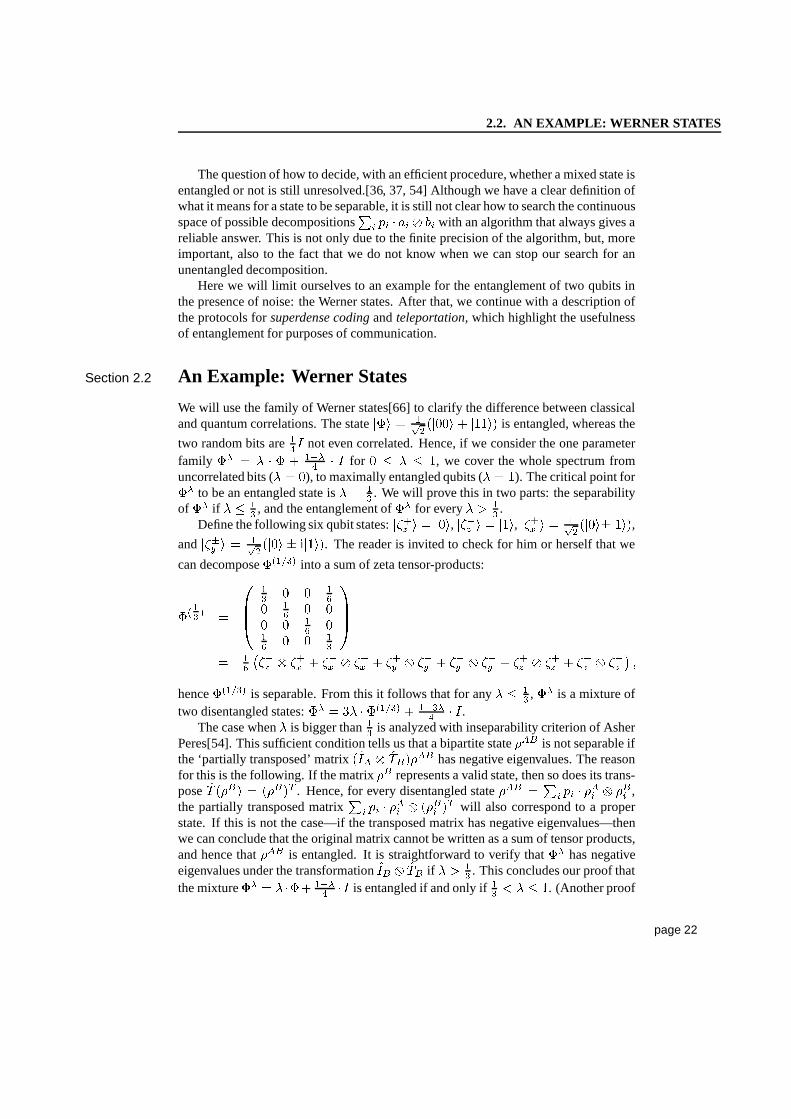
Define the following six qubit states:�� , �� , �� ,

and�� . The reader is invited to check for him or herself that we

can decompose�� into a sum of zeta tensor-products:

��

��

��

��

� ��

hence�� is separable. From this it follows that for any � �� , �� is a mixture oftwo disentangled states:�� .

The case when is bigger than�� is analyzed with inseparability criterion of AsherPeres[54]. This sufficient condition tells us that a bipartite state�� is not separable ifthe ‘partially transposed’ matrix

�� has negative eigenvalues. The reasonfor this is the following. If the matrix�� represents a valid state, then so does its trans-pose �� . Hence, for every disentangled state�� ,the partially transposed matrix�� will also correspond to a properstate. If this is not the case—if the transposed matrix has negative eigenvalues—thenwe can conclude that the original matrix cannot be written asa sum of tensor products,and hence that�� is entangled. It is straightforward to verify that�� has negativeeigenvalues under the transformation�� if � �� . This concludes our proof thatthe mixture�� is entangled if and only if�� . (Another proof

page 22

2.3. SUPERDENSE CODING

of the entanglement of�� can be given in terms of ‘distillable entanglement’. This isdone in [10], where it is shown how one can create near perfectentangled states froman unlimited supply of�� pairs, under the assumption that � �� .)

Section 2.3 Superdense Coding

The procedure of superdense coding shows us how we can transmit two bits of infor-mation with only one qubit. This result was published by Charles Bennett and StephenWiesner in 1992[8], and was one of the first examples of ‘entanglement enhanced com-munication’.

Take two parties Alice and Bob (� and�) that want to communicate with eachother. More specifically, Alice wants to send two classical bits of information to Bobwith a minimum amount of effort. The setting is such that the two parties initiallyshare one entangled pair of qubits�� , and that Alice is allowedto use qubits for her signal, rather than classical bits. Thefollowing single qubit pro-tocol establishes the� bit transmission. (The bits that Alice wants to send are labeled��. The NOT and FLIP operations are unitary, one qubit transformations, definedby NOT

�� and FLIP�� .)

1. Depending on the� and� values, Alice performs the unitary operation NOT� �

FLIP�

to her qubit�� of the entangled pair��. (The qubit that is the result ofthis transformation is indicated by�� .)

2. Next, Alice send her qubit to Bob.

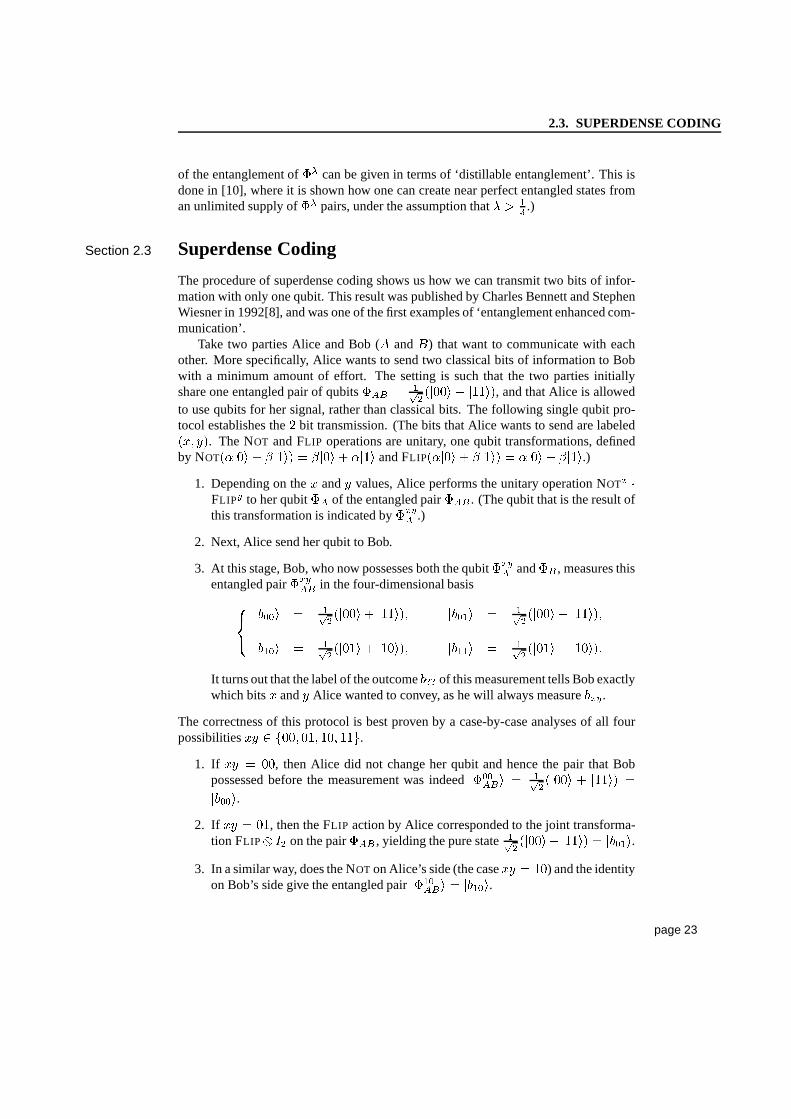
3. At this stage, Bob, who now possesses both the qubit�� and��, measures thisentangled pair�� in the four-dimensional basis

��

��

It turns out that the label of the outcome�� of this measurement tells Bob exactly

which bits� and� Alice wanted to convey, as he will always measure��.

The correctness of this protocol is best proven by a case-by-case analyses of all fourpossibilities�� .

1. If �� , then Alice did not change her qubit and hence the pair that Bob

possessed before the measurement was indeed�� .

2. If �� , then the FLIP action by Alice corresponded to the joint transforma-tion FLIP � � on the pair��, yielding the pure state�� .

3. In a similar way, does the NOT on Alice’s side (the case�� ) and the identityon Bob’s side give the entangled pair

�� .

page 23

2.4. TELEPORTATION

4. The combination of FLIP and NOT on�� results in the state�� , which can be detected with�� reliability, corresponding to the right

answer�� .As the four

�states are mutually orthogonal, no confusion over the outcome is neces-

sary if we assume that Alice and Bob are capable of perfect manipulation, transmissionand observation of their qubits.

Superdense coding shows us how one entangled pair and one qubit of communica-tion can be used to transmit two classical bits of information. The obvious question is:Can we improve this result by either increasing the number ofbits transmitted, or byreducing the resources needed for this protocol? The answeris: No, this is not possible.In the next section, we will collect some of the evidence for this answer by looking attheteleportationprotocol.

Section 2.4 Teleportation

How can we get a qubit across? If we have a perfect quantum channel between twoparties, then we can simply send the quantum information from� to�. But what if wedo not have have this possibility and there is only a classical channel at our disposal?The surprising answer is that the reliable transmission of qubits is still possible if thetwo parties share some entanglement between them. In 1993 Charles Bennett, GillesBrassard, Claude Crepau, Richard Jozsa, Asher Peres and Bill Wootters showed howone entangled pair of qubits and two bits of classical communication are sufficient totransmit an unknown qubit between two parties.[9] (Note that when the properties ofthe qubitare known, a classical description of its parameters can be broadcasted overthe classical channel and no entanglement is required.) This protocol, which has beencoined ‘teleportation’, is in a sense the complement of superdense coding, which usesone entangled pair and one qubit of communication to convey two classical bits ofinformation. The procedure is as follows.

Let Alice have a qubit� that she wants to convey to Bob. Both parties share thestandard entangled pair

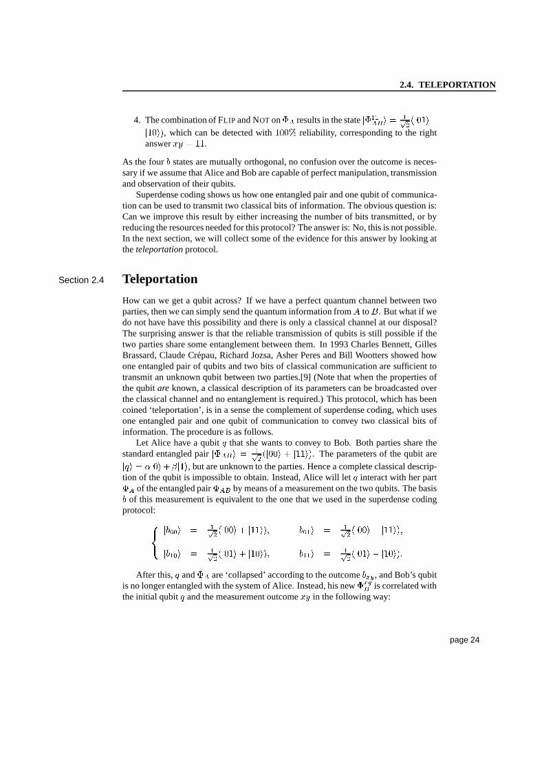
�� . The parameters of the qubit are�� , but are unknown to the parties. Hence a complete classical descrip-tion of the qubit is impossible to obtain. Instead, Alice will let � interact with her part�� of the entangled pair�� by means of a measurement on the two qubits. The basis�

of this measurement is equivalent to the one that we used in the superdense codingprotocol:

��

��

After this, � and�� are ‘collapsed’ according to the outcome��, and Bob’s qubit

is no longer entangled with the system of Alice. Instead, hisnew�� is correlated withthe initial qubit� and the measurement outcome�� in the following way:

page 24

2.5. INFORMATION VERSUS INFORMATION REPRESENTATION

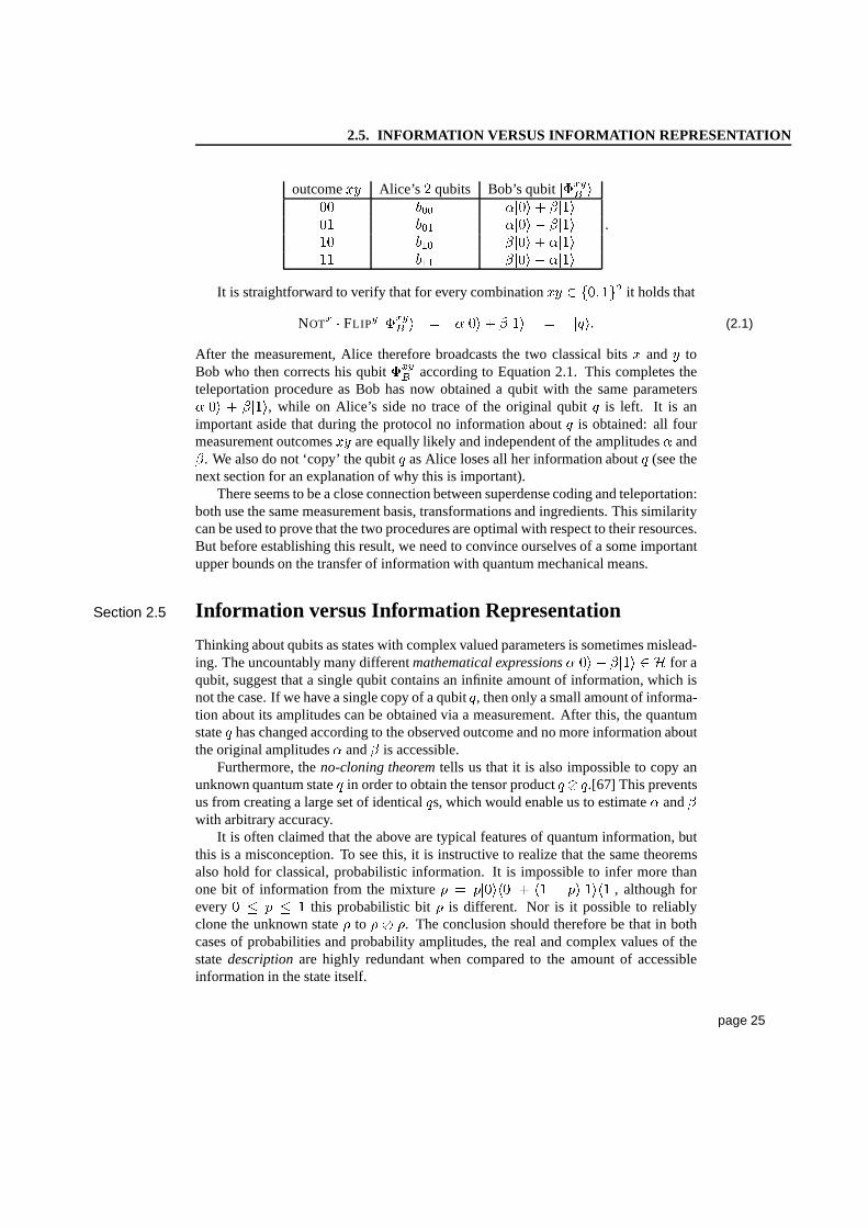
outcome�� Alice’s � qubits Bob’s qubit��

��

.

It is straightforward to verify that for every combination�� it holds that

NOT� �FLIP

� �� (2.1)

After the measurement, Alice therefore broadcasts the two classical bits� and � toBob who then corrects his qubit�� according to Equation 2.1. This completes theteleportation procedure as Bob has now obtained a qubit withthe same parameters�� , while on Alice’s side no trace of the original qubit� is left. It is animportant aside that during the protocol no information about � is obtained: all fourmeasurement outcomes�� are equally likely and independent of the amplitudes� and�. We also do not ‘copy’ the qubit� as Alice loses all her information about� (see thenext section for an explanation of why this is important).

There seems to be a close connection between superdense coding and teleportation:both use the same measurement basis, transformations and ingredients. This similaritycan be used to prove that the two procedures are optimal with respect to their resources.But before establishing this result, we need to convince ourselves of a some importantupper bounds on the transfer of information with quantum mechanical means.

Section 2.5 Information versus Information Representation

Thinking about qubits as states with complex valued parameters is sometimes mislead-ing. The uncountably many differentmathematical expressions�� for aqubit, suggest that a single qubit contains an infinite amount of information, which isnot the case. If we have a single copy of a qubit�, then only a small amount of informa-tion about its amplitudes can be obtained via a measurement.After this, the quantumstate� has changed according to the observed outcome and no more information aboutthe original amplitudes� and� is accessible.

Furthermore, theno-cloning theoremtells us that it is also impossible to copy anunknown quantum state� in order to obtain the tensor product� ��.[67] This preventsus from creating a large set of identical�s, which would enable us to estimate� and�with arbitrary accuracy.

It is often claimed that the above are typical features of quantum information, butthis is a misconception. To see this, it is instructive to realize that the same theoremsalso hold for classical, probabilistic information. It is impossible to infer more thanone bit of information from the mixture� � � �� , although forevery

� � � � � this probabilistic bit� is different. Nor is it possible to reliablyclone the unknown state� to � � �. The conclusion should therefore be that in bothcases of probabilities and probability amplitudes, the real and complex values of thestatedescriptionare highly redundant when compared to the amount of accessibleinformation in the state itself.

page 25

2.6. HOLEVO’S BOUND AND AN APPENDIX TO IT

It is the combination of superpositions with the phenomenonof interferencethatmakes the crucial difference between classical and quantuminformation. The possi-bility of the superpositions�� and �� to evolve to the different

pure states�� and

�� (after a Hadamard transform), somehow suggests that a quantummechanical superposition is more ‘real’ than the probabilistic combination of two bitvalues. It seems as if for a qubit�� , both states are really present, whereasin the probabilistic case, the mixture� �� ‘in reality’ has alreadydecided which binary value it represents. But this does not allow us to confuse a quan-tum mechanical superposition with its deterministic description as a density matrix ona piece of paper. Such confusion leads too easily to an overestimation of the inherentcomplexity of a single quantum state.

Section 2.6 Holevo’s Bound and an Appendix to It

A more accurate analysis on the limitations of qubits to carry classical information isprovided by Alexander Holevo’s theorem on quantum sources[35] and an addendum tothis result by Michael Nielsen (see the original [24] and theappendix of thesis).

For the purpose of this thesis we will focus here on the latter, but the reader isencouraged to familiarize him or herself with Holevo’s result as well as with a recentgeneralization of this theorem by Ashwin Nayak[48].

Nielsen’s result reads as follows. If Alice wants to transmit � bits of informationto Bob and� and� start as unentangled systems, then this can only be done withatleast� (quantum) bits of communication between the two parties. This can be furtherspecified as a lower bound on the amount of communication fromAlice to Bob (being�� qubits), and on the total amount of communication,�� . (where�� isthe number of qubits that Bob sends to Alice during the protocol). The bounds are inaccordance with what we already know to be possible with superdense coding:

� For the communication from Alice to Bob:�� .

� For the total amount of communication:�� .

We can reach Nielsen’s bounds if we let Bob distribute�� (with �� ) entan-

gled pairs by sending�� qubits to Alice, who then uses�� qubits for superdensecoding and� � �� qubits for traditional communication. For every allowed valueof ��, this protocol indeed uses�� (quantum) bits from Aliceto Bob, and�� qubits in total.

Section 2.7 Optimality of Superdense Coding and Teleportation

A direct consequence of Nielsen’s bound is that when Alice sends � qubits to Bob,she can only convey�� classical bits of information. This, in combination with theprotocols for superdense coding and teleportation, gives the following useful limits:

1. If Alice and Bob share initial entanglement and Alice sends� classicalbits, thenonly � bits of information can be transmitted from Alice to Bob.

page 26

2.7. OPTIMALITY OF SUPERDENSE CODING AND TELEPORTATION

2. Superdense coding cannot be used to transmit more than twoclassical bits perqubit.

3. It is impossible to teleport a qubit with less than two classical bits of communi-cation from Alice to Bob.

These three results are easily proven by the strong similarity between superdense cod-ing and teleportation. Respectively:

1. By running two such protocols in parallel, Alice would be able (using superdensecoding) to replace her�� classical bits with� qubits. Hence we would have aprotocol with �� that transmits more than�� bits of information fromAlice to Bob. This is impossible.

2. This is a specific instance of Nielsen’s result.

3. Assume that strictly less than� bits are necessary. For big enough� it shouldthen be possible to teleport� � � qubits with�� classical bits. Hence, if wewould use the� � �qubits as part of a superdense coding procedure, we wouldtransmit more than�� bits with �� bits of classical information. This is notpossible by the first result.

The preceding sections seems to suggest that the differencebetween quantum andprobabilistic bits is ‘a factor of two’ and that teleportation and superdense coding sum-marize everything there is to know about (errorless) quantum communication. The factthat there are many more pages to follow in this thesis indicates that this is not the case.In the next chapter we will touch on a much discussed feature of quantum mechanics:nonlocality. We will see that there is a fundamental difference between the classicaland the quantum theory of information after all, and that isby definitionthat there isno classical explanation of the ‘nonlocal’ correlations that are possible with entangledqubits.

page 27

Chapter 3

Nonlocality

In this chapter the issue of nonlocality is discussed. We look at how local hiddenvariable theories put a limit on the correlations that they can describe. The predictionsof quantum mechanics violate these bounds, which tells us that the theory of quantumphysics does not have a local, probabilistic model. Specialattention is paid to theso-called ‘loopholes’ of experiments that try to verify thenonlocality of Nature.

Section 3.1 Bell’s Inequality

It was in 1964 that John Bell gave a new impulse to the discussion on the foundationsof quantum mechanics with his celebrated inequality of locality.[6, 7] Ever since then,other such inequalities have been derived, corresponding experiments have been per-formed, and heated debates are still being held about the exact implications of it all. Itis the opinion of this author that the most important thing tounderstand about Bell’sinequality is that does not try to say anything about the theory of quantum physics.Instead, it puts a general bound on all possible classical, local models for Nature. Af-ter the derivation of this bound there are two kinds of (possible) violations that drawour attention. The first one is themathematical factthat conventional quantum me-chanics gives predictions that are not possible to describewith a classical model. Theexperimental verificationof the violation of the inequalities is the second and mostimportant aspect of Bell’s result. It is because of this dichotomy between theory andexperiment that the nonlocality of Nature can be verifiedindependentlyof the validityof our current theory of quantum mechanics.

Section 3.2 Classical or Hidden Variables Models

Crucial to a proper understanding of quantum nonlocality isthe definition of what ismeant withclassical locality.In this thesis we adopt the (arguably conventional) inter-pretation of the terms ‘local, realistic theory’ and ‘hidden variable model’, which bothrefer to the same set of classical assumptions about a system. To avoid any unnecessaryconfusion, we will define these terms below.

page 28

3.2. CLASSICAL OR HIDDEN VARIABLES MODELS

When measuring a physical system��, we observe certain outcomes with certainprobabilities. Without loss of generality we assume here that we always have binaryoutcomes “yes” (�) or “no” (

�). The probability of obtaining the answer “yes” when

performing the measurement on system�� is denoted by��

��. A range ofdifferent measurements, �, � � � on the same system leads to a corresponding rangeof probabilities

�� , ��

��, � � � We speak of adeterministic system�

if for each measurement�, the outcome is completely predetermined. In this case,�� is always an element of�� ; and hence, with� different measurementsettings (� � �� ), there are�� different deterministic systems.

A probabilistic system�� is a mixture of deterministic systems�� (indexed by�),

with the probability distribution�: “ �� ”. A measurement on sucha mixture �� will therefore give the answer “yes” with probability

�� . (Note that for the distribution�, it holds that�� and��

.) Just as the outcomes�� for deterministic systems are

predetermined, so are the probabilities��

��completely specified in advance bythe distribution�. This is the ‘realistic’ part of traditional theories: every characteristicthat one can measure about a system is already described (‘isreal’) in that systembefore the actual measurement.

Consider now a deterministic bipartite system�� that is distributed over Alice(whose subsystem is labeled��) and Bob (with his��). A model for��’s behavioris considered ‘local’ if nothing outside the measurement setting � and the state��can influence the outcome of this specific experiment. This means that even though�� was once part of a larger system��, �� by itself contains all the informationabout the way it will ‘react’ to the measurement�. For two different measurements�� and� there are� deterministic subsystems�� . The same applies for exper-iments done by Bob on his part��. From this it follows that we have�� possiblestates�� if �� has to give a local and deterministic descriptionfor the combinations of separated experiments

�� , �� , �� and

�� . Note that when we drop the locality requirement, each experimenthas four possible outcomes, leading to much more,�� , different deterministicmodels.

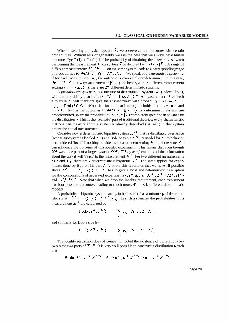
A probabilistic bipartite system can again be described as amixture� of determin-istic states: �� . In such a scenario the probabilities for ameasurement� are calculated by

��

and similarly for Bob’s side by��

The locality restriction does of course not forbid the existence of correlations be-tween the two parts of��. It is very well possible to construct a distribution� suchthat

�� page 29

3.3. TWO-PARTY NONLOCALITY

If there is a local, realistic theory for a system, then the behavior of this �� iscompletely specified by its underlying distribution. Such atheory is therefore alsocalled a ‘hidden variable model’, where the variables are understood to be definingfunction�. Bell’s inequality gives us a limit to what is possible with systems that admitsuch a classical description.

Section 3.3 Two-Party Nonlocality

I will present here the variant of Bell’s inequality as it wasphrased by John Clauser,Michael Horne, Abner Shimony and Richard Holt in 1969: theCHSH inequality.[22]The traditional labeling with spin directions is replaced with an equivalent descriptionin bit values as this is how we will use the result later in the thesis.

Consider two separated parties� and� who both receive a subsystem�� and��. Each side chooses to perform one out of two experiments:�� or �� on Alice’sside, and�� or �� for Bob’s part. This procedure is repeated many times suchthat all four possible measurement settings can be examined. We are interested in thecorrelated (�� ) and anti-correlated (�� ) outcomes for those fourpossibilities. By using binary values in combination with modulo two arithmetic (with��

), we can rewrite these (anti)-correlations as

� �� if the outcomes� and� are correlated,

� if the outcomes� and� are anti-correlated.

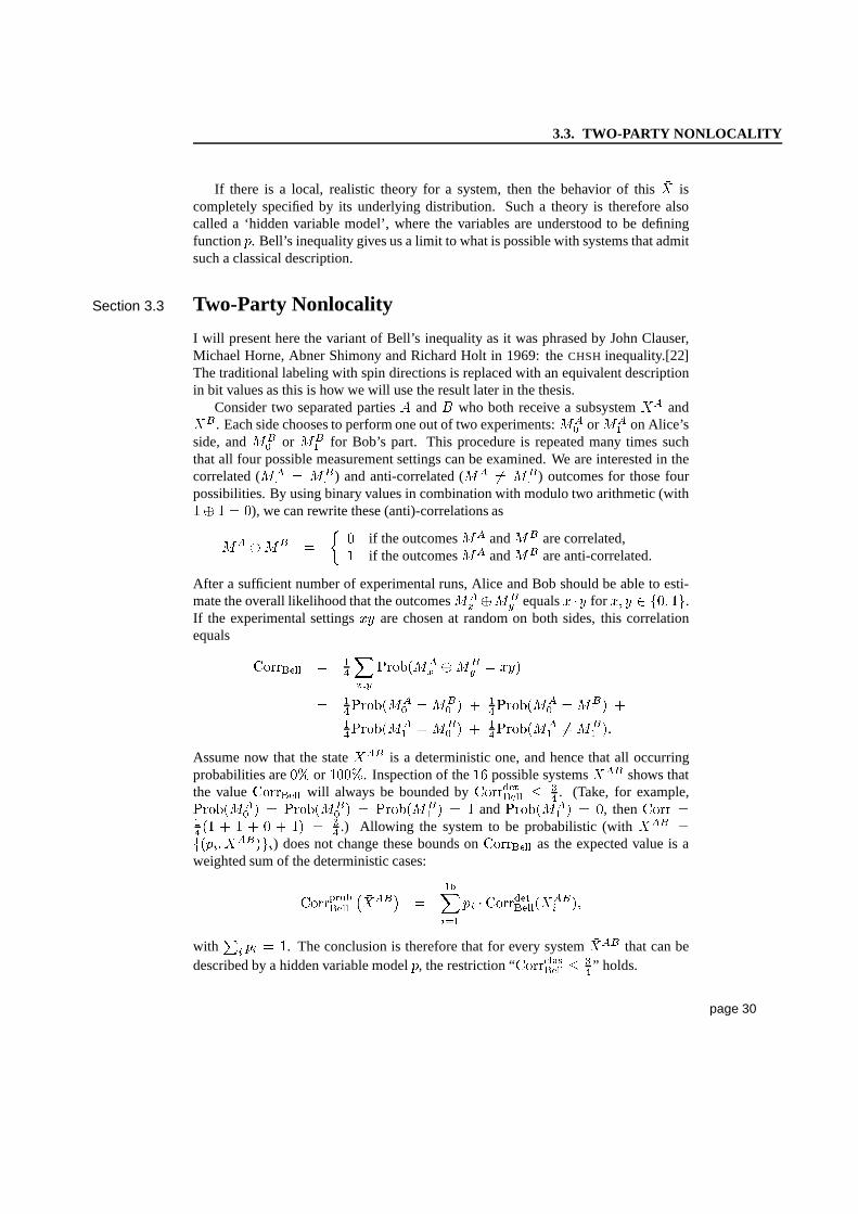
After a sufficient number of experimental runs, Alice and Bobshould be able to esti-mate the overall likelihood that the outcomes�� equals� �� for �� .If the experimental settings�� are chosen at random on both sides, this correlationequals

��

��

� �� Assume now that the state�� is a deterministic one, and hence that all occurringprobabilities are

��or ��. Inspection of the�� possible systems�� shows that

the value�� will always be bounded by

�� . (Take, for example,�� and

�� , then

�� .) Allowing the system to be probabilistic (with��

�� ) does not change these bounds on�� as the expected value is a

weighted sum of the deterministic cases:

��

��

with �� . The conclusion is therefore that for every system�� that can bedescribed by a hidden variable model�, the restriction “

�� ” holds.

page 30

3.4. THREE-PARTY NONLOCALITY

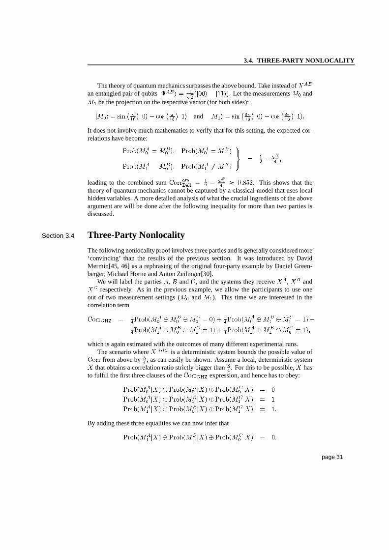
The theory of quantum mechanics surpasses the above bound. Take instead of��an entangled pair of qubits

�� . Let the measurements� and� be the projection on the respective vector (for both sides):

�� and��

It does not involve much mathematics to verify that for this setting, the expected cor-relations have become:

��

��

��

� �

leading to the combined sum��

� � ��. This shows that thetheory of quantum mechanics cannot be captured by a classical model that uses localhidden variables. A more detailed analysis of what the crucial ingredients of the aboveargument are will be done after the following inequality formore than two parties isdiscussed.

Section 3.4 Three-Party Nonlocality

The following nonlocality proof involves three parties andis generally considered more‘convincing’ than the results of the previous section. It was introduced by DavidMermin[45, 46] as a rephrasing of the original four-party example by Daniel Green-berger, Michael Horne and Anton Zeilinger[30].

We will label the parties�, � and�, and the systems they receive��, �� and�� respectively. As in the previous example, we allow the participants to use oneout of two measurement settings (� and�). This time we are interested in thecorrelation term

��

which is again estimated with the outcomes of many differentexperimental runs.The scenario where�� is a deterministic system bounds the possible value of

�� from above by�� , as can easily be shown. Assume a local, deterministic system

� that obtains a correlation ratio strictly bigger than�� . For this to be possible,� has

to fulfill the first three clauses of the�� expression, and hence has to obey:

��

By adding these three equalities we can now infer that

�� page 31

3.5. LOCALITY LOOPHOLES

(We used here the fact that all probabilities are zero or one and thus��

�� for any .) This conclusion contradicts the fourth clause of the

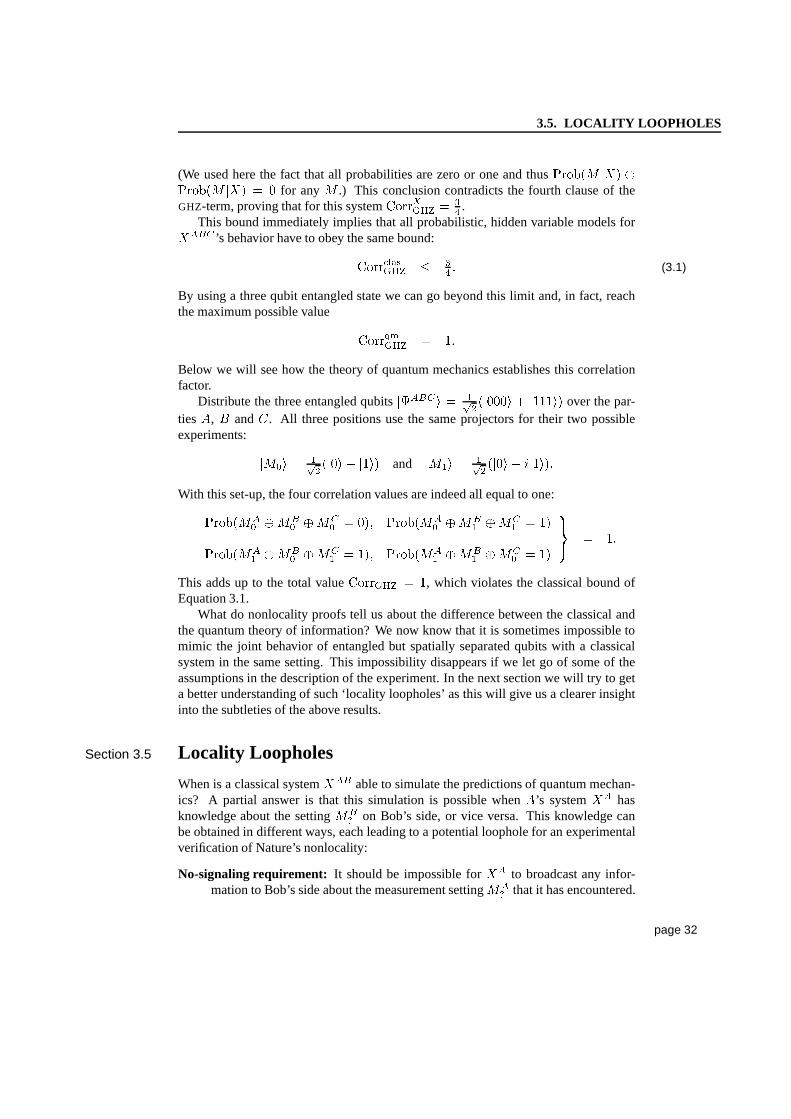
GHZ-term, proving that for this system��

� .This bound immediately implies that all probabilistic, hidden variable models for

��’s behavior have to obey the same bound:

�� (3.1)

By using a three qubit entangled state we can go beyond this limit and, in fact, reachthe maximum possible value

�� Below we will see how the theory of quantum mechanics establishes this correlationfactor.

Distribute the three entangled qubits�� over the par-

ties�, � and�. All three positions use the same projectors for their two possibleexperiments:

�� and��

With this set-up, the four correlation values are indeed allequal to one:

��

��

This adds up to the total value�� , which violates the classical bound of

Equation 3.1.What do nonlocality proofs tell us about the difference between the classical and

the quantum theory of information? We now know that it is sometimes impossible tomimic the joint behavior of entangled but spatially separated qubits with a classicalsystem in the same setting. This impossibility disappears if we let go of some of theassumptions in the description of the experiment. In the next section we will try to geta better understanding of such ‘locality loopholes’ as thiswill give us a clearer insightinto the subtleties of the above results.

Section 3.5 Locality Loopholes

When is a classical system�� able to simulate the predictions of quantum mechan-ics? A partial answer is that this simulation is possible when �’s system�� hasknowledge about the setting�� on Bob’s side, or vice versa. This knowledge canbe obtained in different ways, each leading to a potential loophole for an experimentalverification of Nature’s nonlocality:

No-signaling requirement: It should be impossible for�� to broadcast any infor-mation to Bob’s side about the measurement setting�� that it has encountered.

page 32

3.5. LOCALITY LOOPHOLES

The no-signaling requirement is fulfilled if both measurements� and� arespace-like separated events in space-time. Special relativity then tells us then thatno information can travel between the two acts of measurement. Note that thisspace-like separation is only a method to establish the no-signaling condition.It would be equally valid if we were able to prohibit the transfer of informationbetween� and� by other means.

Unpredictable measurement settings:The transfer of information between the twoparties is unnecessary if the measurement settings are known to the systems��and �� from the start. It is straightforward to reproduce the statistics of quantummechanics if the four different experimental settings�� occur in a regularpattern that can be predicted by the system�� before it separates into twosubsystems. The choice on both sides should therefore be made at random andindependently of each other. (The independence can again beestablished bymaking the two decisions at space-like separated events.)

Besides the aforementioned two restrictions, there is a third, more practical, way fora model to mask its classical foundations: the detector efficiency loophole. In practiceit will almost never be the case that every signal can be detected by the measurementapparatus. As an example, with current technology, the detection of both the polariza-tions of entangled photons succeeds with a success probability of less than one percent.In such situations it is possible to come up with a classical model where the photonsonly ‘reveal’ themselves at� and� if the setting of the devices is in accordancewith a scheme that was agreed upon before�� and �� parted. When one of the pho-tons encounters an undesired setting, this particle then ‘hides’ itself from the detector,resulting in just one of the many unsuccessful polarizationmeasurements. Such (ad-mittedly contrived) ‘conspiracy theories’ are able to givea local explanation for all theperformed nonlocality experiments to date.[52]

The reader might wonder what the practical merits are of these academic objec-tions to the acceptance of nonlocality as a feature of Nature. After all, if our quantumcommunication protocol works as desired, why contemplate the ins and outs of themodel that describes it? The surprising counter argument tothis critique is that theabove conditions translate directly into the requirementsfor a quantum protocol thattruly outperforms the classical ways of processing information. This is the excitingidea behind quantum communication as I will discuss it in this thesis: to use Nature’snonlocality to save on the amount of communication that is necessary in certain set-tings.

In the next chapters, we will see how the above arguments about the foundationsof quantum mechanics can be transformed into procedures that reduce the complexityof distributed calculations. But before we are able to do this, it will be necessary tointroduce a notion from computer science: communication complexity.

page 33

Chapter 4

Communication Complexity

In this chapter we introduce the notion ofcommunication complexity.It is first definedin the traditional, classical sense after which we expand itto the quantum case. Alsothe generalization to multiple parties is made. Special attention is paid to the notionof probabilistic protocols and how they can be viewed as mixtures of deterministiccommunication procedures.

Section 4.1 Introduction

Consider two remote parties Alice and Bob each in possessionof data that is unknownto the other person. If Alice has a natural number� and Bob has�, how many bits doesBob have to send to Alice such that she will be able to determine if � � � is even orodd? Clearly this can be done with a single bit of informationas Alice (who knows�)is only interested in whether or not Bob’s� is even or odd. But what if Alice wants todecide if�� is prime? Intuitively one expects that in order to determinethis decisionproblem, Alice and Bob will have to exchange more information than the previous onebit, and that this amount of communication will depend on thesizes

�� and�� of the

input strings. But how will it depend on the input size? What is the most efficientprotocol? And given this optimal solution, how do we prove that there does not exista better procedure? The theory ofcommunication complexitytries to answer questionslike these.

Section 4.2 Two-Party Communication Complexity

The setting for communication problems where there are two cooperative parties whowant to compute a joint decision problem is as follows.

Alice and Bob are given two strings� and� respectively, both of length�. Theywant to compute a Boolean function

�on these two input strings, hence for a given�,

the function�

will be of the form�� . The communication

complexity of this function is the minimal amount of communication between the two

page 34

4.3. SOME OBSERVATIONS ABOUT COMMUNICATION COMPLEXITY

parties that is necessary for Alice to calculate the binary value��. More precisely,

the complexity of the distributed task�

is expressed by the relation between the inputsize� and the amount of communication necessary for the evaluation of

�� for

the worst case input strings� and�. The following observations should clarify thisdefinition.

Section 4.3 Some Observations about Communication Complexity

The trivial example of the “�� even or odd?” problem in the beginning of this chapteris one of the simple cases where the communication complexity is constant and henceindependent of the input size. The version where Alice triesto determine the primalityof � � � has the obvious upper bound of� (which holds forany

��), because Bob can

always send all his� bits to Alice who then finishes the computation “� � � prime?”on her side. This underlines the fact that thecomputational difficultyof determiningthe function PRIME (or any other function

�) does not play a role here.

Because of the worst case assumption, the following line of reasoning is incorrect:“The sum� � � will be even (and hence composite)

��of the time. This can be

checked with a single bit of communication; therefore, the average communicationcomplexity of the PRIME� problem will be less or equal to� .” Instead, we shouldconclude that the complexity of PRIME is going to be determined by the values of�and� for which their sum is not divisible by two.

The fact that Bob does not have to know the answer after the protocol does not haveany significant consequences: it will only require one additional bit of communicationfor Alice to tell the final answer

� �� to Bob.

Section 4.4 Formal Definition of Deterministic Communication

A deterministic protocol�

fully determines for every possible input�� which party

is going to communicate which bit at what stage of the protocol. At the start of theprocedure, the parties are unaware of each others inputs; therefore, who is going tocommunicate the first bit has to be ‘input independent’ (and hence pre-determined). Ifwe assume that this is Alice, then she has to act according to two decision sets�� and�� in that she sends a “zero” to Bob if and only if her input� � ��, and a “one” if andonly if � � ��. Because we require the protocol to be unambiguous and well-definedfor every�, it follows that�� is emptyand that�� covers the whole set ofpossible inputs for Alice. For the second bit, the situationbecomes more complicatedas we now have the two situations where the first communicatedbit was zero or one.We will make this distinction by putting the relevant history of communication in theupper indices of the decision sets. Hence, we could have the description in the formof the two couples

�� and�� , which would tell us that depending on the

first bit, Alice or Bob announces the second bit. More specifically, if the first valuewas zero, then Alice continues according to the sets�� and��. Otherwise, Bob useshis decision sets�� and��. Again, each couple of sets obeys the above-mentionedrestrictions for a deterministic protocol. In general, we will completely specify what

page 35

4.4. FORMAL DEFINITION OF DETERMINISTIC COMMUNICATION

happens after Alice and Bob have communicated the string� � �� by either apair

�� if Alice has to communicate the next bit, or�� if it is Bob’s turn.

Notice that it is not possible to have a combination of�� and�� as this makes itambiguous who is going to communicate. At the end of the protocol it is Alice whohas to determine the function value

� ��. Similarly, we can represent this with twodecision sets for�, as long as we understand that this time the lower index denotes thefinal decision and is no longer part of the communication.

We can visualize a deterministic protocol as a decision treewhere the nodes arelabeled by the strings� that express the ‘communication so far’ and the branches bythe respective decision sets��, ��, et cetera. Figure 4.1 shows such a tree for a simplethree bit communication protocol, which we shall use for thefollowing example.

Imagine a two-party protocol�

where both Alice and Bob receive two bits (��,�� ) that is described by:

1. If Alice has�� , then she sends a “zero” to Bob, who then knows that the

protocol has ended.

2. Otherwise, Bob will receive the value “�” from Alice, telling him that he has tocommunicate back both his input values�� and�.

3. After the communication has ended, Alice calculates the outcome of the proto-col:

�� is the bit value�� . She is able to do this either because�� , or on the basis of her knowledge of Bob’s two input bits�� and� (in

combination with her own input��).A description such as the one above easily becomes unclear for larger protocols.

It is for this reason that we use the formalism of decision sets. The three steps of theabove example are thus summarized by the pairs of sets:

1. Alice’s sets�� and�� .2. Bob’s first bit with�� and�� ; his second bit:��

�� and�� .3. And the final conclusion of Alice by the table:

�� and �� .

Notice that the ‘completeness requirement’ for the union�� sometimes leads to a redundancy in the sets as they cover input states that do not applyto them. (For example, the fact that��

is an element of�� , which only isused when�� .) By the tree construction we also see that the strings�� of thefinal conclusion sets for Alice form a complete, self-delimiting code such that no�� isthe prefix of another string�� , and any sufficiently long bit string starts with one of thewords��.

page 36

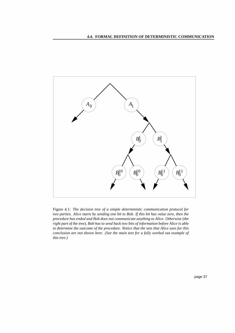
4.4. FORMAL DEFINITION OF DETERMINISTIC COMMUNICATION

AA 10

01B 1B

0B 0B0B0B

1

10 10 11 11

Figure 4.1: The decision tree of a simple deterministic communication protocol fortwo parties. Alice starts by sending one bit to Bob. If this bit has value zero, then theprocedure has ended and Bob does not communicate anything toAlice. Otherwise (theright part of the tree), Bob has to send back two bits of information before Alice is ableto determine the outcome of the procedure. Notice that the sets that Alice uses for thisconclusion are not shown here. (See the main text for a fully worked out example ofthis tree.)

page 37

4.5. PROBABILISTIC PROTOCOLS

The two important characteristics of decision trees and their sets that we mentionedearlier will be repeated here formally.For a deterministic protocol that calculates afunction

�� , the decision sets have to obey the following:

1. Every occurring node� � �� in the tree either contains a pair�� or�� .

2. For every pair�� it holds that�� and�� .

3. All the ‘leaves’ (or end nodes) of the tree are� pairs as these contain the con-clusion of Alice after she has completed the communication with Bob.

The amount of communication before Alice’s conclusion corresponds exactly withthe length

��of the string� that labels the leaves��. The worst case assumption tells usthat the communication complexity of a protocol is the longest possible� that appearsin a leaf. This is identical with the depth of the decision tree, minus one. Our tree-example for the calculation of the function�� therefore has complexity�, despite the fact that for the case��

, it only requires one bit of communication.

Section 4.5 Probabilistic Protocols

We speak of a probabilistic solution if the parties use a protocol that gives Alice thecorrect answer

� ��with high probabilityfor all combinations��. The minimum

correctness ratio�� (a protocol with probability of error�) will in general influencethe amount of communication that is necessary to obtain the confidence level. With� � �

we obviously return to the deterministic case.An important aspect of the definition lies in the phrase “for all combinations

��”which I will clarify here. Imagine a deterministic protocol

�that is successful for all

possible input combinations�� except one. At first glance this may seem a reliable

solution of the problem. But the worst-case assumption tells us, in fact, that with thisprotocol

�, we should expect the values� and� for which the procedure fails. This

teaches us that if there is an input on which a deterministic procedure makes an error,then this protocol has to be considered useless (the error� equals�). For a successfulprobabilistic approach, we need to add randomness as one of our ingredients.

The reason that our deterministic protocol failed was because its errors were alsodeterministic and hence predictable by the worst-case distribution � that specifically‘aims’ at the weak spots of proposed solutions. We counter this by randomizing theerrors ourselves in the sense that we try to ‘spread out’ the values

�� for which weare likely to make a mistake. Such an approach requires Aliceand Bob to share somerandom bits on the basis of which they execute their otherwise deterministic protocol.The following example should be instructive.

Assume that Alice and Bob try to calculate the distributed function�

� � ��

�� (where� stands for the set of input values�� ). Imagine that for each�� there exists an efficient deterministic protocol�� that works correctly

except for the one combination�� . That is, every protocol

�can make a

mistake, but the protocols differ inwherethey err. This allows� and� to adopt thefollowing strategy:

page 38

4.5. PROBABILISTIC PROTOCOLS

1. Alice receives�, Bob receives his� ��.

2. Both parties agreeat randomon a pair�� that determines which one of the�

protocols�

they are going to execute.

3. Alice and Bob perform the deterministic protocol�� .

(Note that the random bits (� �� in total) are usedbeforethe actual communica-tion procedure.) Unlike the earlier non-randomized approach, this protocol is highlysuccessful, as we can easily see. Given any combination

��, Alice and Bob haveprobability �

�� that they ended up executing the flawed protocol�� for this specific

input. We have the remaining probability of�� that the two parties performed one

of the� � �procedures�

that leads to the right answer� ��. For reasonably large�, this will occur with high probability. As it is impossible for the distribution of the

input values to ‘anticipate’ the protocol�� that� and� are going to perform, it is

also impossible to force an error rate higher than the�� that holds for this probabilistic

solution.A few more words about the random bits that the parties use before we give our

final characterization of probabilistic communication protocols. The randomizationthat we saw in the last example wasshared randomness:both parties could agree on therandom numbers

�� without having to communicate this specification to each other.This is also called the ‘public coin model’ of communicationand can be viewed asthe situation where Alice and Bob share an unlimited amount of classically correlatedstates

�� A more restricted model of randomized communication is the one where the partiesonly have ‘private coins’. In this model, shared randomnesscan only be achievedafter one party has communicated some of his or her coin flips to the other participant.Hence, in this ‘private coin’ model we have to take into account the amount of sharedrandomness that the parties have to send to each other for thesuccessful execution oftheir randomized procedure. In this thesis, we will always assume the ‘public coin’model for reasons that will be explained in Section 4.10.

Another issue is that of the moment of randomization in the protocol. If we knowbeforehand the outcomes of all the random coin flips that willoccur during a protocol,then we can again view the procedure as a deterministic one. And because there isnothing during the protocol that can influence the outcome ofa coin flip, we might aswell observe all of them before we start with the procedure

�. As long as we establish

our randomizationafter we received the� and� values, the input distribution cannot‘anticipate’ any weaknesses specific for the outcomes of thecoin flips.

It is for the above reasons that we can assume, without loss ofgenerality, that theprobabilistic protocol

�is executed according to the three steps previously shown:

1. The parties receive their respective inputs.

2. With the help of public coin flips, Alice and Bob agree on a random number�

(according to some fixed distribution�).

page 39

4.6. AN APPLICATION OF VON NEUMANN’S MIN-MAX THEOREM

3. The deterministic protocol�� is executed.

This can be summarized by the statement that the probabilistic procedure�

is a mixtureof deterministic protocols,

� � �� , and that on the input strings��, it

outputs the corresponding probabilistic bit� �� .

The quest for the optimal probabilistic protocol for a function�

can be approachedin two ways:

Given a desired success rate�� , how many bits of communication are required?

Or alternatively:

What is the minimum error rate� that can be obtained with� bits of communication?

Although both kinds of questions will be asked in the coming chapters, we will hereinvestigate problems of the second kind. The next section will show us how we canemploy some standard techniques from game theory for our analysis of communicationcomplexity.

Section 4.6 An Application of Von Neumann’s Min-Max Theorem

Consider again the setting that we described before we endedthe previous section.Alice and Bob want to calculate the distributed function

��

�� with only � bits of communication between them. Our task is to optimize theirrandomized protocol in that we want the highest possible success ratio� � � for thislimited amount of communication�. What do we do if every deterministic protocol(with � � �

) requires more than� bits of communication?As we now know, every probabilistic protocol

�can be expressed as a mixture

�� , where� is the defining probability distribution over the set ofall the de-terministic protocols

��. (Typically, we will have�� for many unreliable proto-

cols��.) Our second relevant distribution is the function� that defines the probability

�� that Alice and Bob receive the input pair

��. Given the distributions�(defining the protocol

�) and� we calculate the error rate by

��

��

� ��

�� where� is the ‘difference function’ with��

if� �

and�� other-wise. The worst case assumption for the input distribution can now be expressed as themaximization of the error over all�’s:

�� But we, in the meantime, are looking for the protocol

�thatminimizesthe error, and

hence we are trying to reach the minimum of this maximum error, which is

��

��

page 40

4.6. AN APPLICATION OF VON NEUMANN’S MIN-MAX THEOREM

where�

is the problem in question, and all�� are deterministic protocols. This is the

situation from the viewpoint of Alice and Bob.Nature, with her worst case behavior, on the other hand, aimsfor the highest possi-

ble error for each protocol�

. This corresponds to an expression that is almost identicalto the previous one,

��

except for the changed order of the two optimizations.This puts us in the situation where we have to analyze two conflicting strategies:

the minimization of� by Alice and Bob, and the maximization of the same term byNature. It is therefore legitimate to ask if the whole setting is properly defined; forit is not inconceivable that the chain of arguments “Alice and Bob use protocol

�”,

“Nature reacts by using the worst possible distribution�”, “knowing this specific�,the two parties change to a better

��”, “Nature counters with a new��”, et cetera,

has no well-defined end. Luckily, Andrew Yao’s usage of Von Neumann’s Min-Maxtheorem assures us that this is not the case, as there is a fixedpoint

�� for thisproblem. (See the article [68] and the references [47, 49, 50, 51] for an introduction togame theory.)

It turns out that the above setting is an example of a ‘zero-sum, two player game’.Let the first player be the duo Alice & Bob with their protocol

�, and the opposing one

Nature with her strategy�. We can rephrase the conflicting goals for the participantsby stating that Nature tries to maximize the error�, whereas Alice and Bob try tomaximize the negated term “��”. This indeed makes it a zero sum game (for twoplayers), and hence Von Neumann’s celebrated Min-Max theorem applies. This resultstates that in the just-described setting there is always a fixed point

�� (a solutionof the game), such that the corresponding� (the uniquevalueof the game) solves theequation

�� As this defines asaddle point,both parties know that any variation in their strategy(� for � and�, and� for Nature) is not going to do them any good because, for thesolution of the game, it holds that

For any alternative protocol��, we obtain an error that cannot be smaller.

All other input distributions�� give an error that cannot be bigger.

In short,�� and��

� �� , for all �� and��.

(Note that it is very well possible that several solutions exist for a game, but all of themwill share the same value�.) The above two characteristics in combination with thedecomposition of a probabilistic protocol as a mixture of deterministic ones, also givesus a technique to easily ‘recognize’ the fixed-point solution of a setting. This will beexplained in the next section.

page 41

4.7. PROVING PROBABILISTIC BOUNDS

Section 4.7 Proving Probabilistic Bounds

We now know that for every probabilistic communication setting, there is a solution inthe form of an ideal protocol

�, a worst case input distribution� and the resulting error

rate�. But how do we determine such a solution? As stated earlier inthis thesis, we aremainly interested in the setting where we try to minimize theerror under a restrictionon the amount of communication. In this setting, a relevant probabilistic protocol

�will have to be a mixture�� of deterministic procedures

�� that all obey thislimitation on the information transfer between Alice and Bob. Hence, if we can exhibita specific input distribution� and an error rate

�for which every alloweddeterministic

protocol�� obeys

��

then we can immediately conclude that anyprobabilistic protocol�

will obey thisbound

�as well. And because� is the maximum of� �� overall distributions�, we

now also know that�

is a lower bound on the value�. In mathematical terms, thisreasoning can be summarized by

� � �� Conversely, if we can prove for the same

�the existence of a protocol

�that obeys

�� for every input distribution� and hence��

, then we can conclude that� � ��

. (The proof of this “��

” is usually done by showing that forevery pair

��, the error probability of the protocol�

is limited by��

.)The combination of the two bounds shows that indeed� � �

, and the solutionfor this value is obtained by the distributions� and� that we used in the proof. Inpractice, it will almost always be the case that we simply suggest a distribution� forwhich it is easy to verify that everydeterministicprotocol has an error rate of at least�. After that lower bound, we then continue by describing a probabilistic protocol with�� for every input pair

��. This is sufficient to provethat

�� is a solution of the communication game with value�. (It is typical forthe worst-case distribution� that it will be zero for any couple

�� for which theprotocol performs above average.)

Some readers might find it unsatisfying that we just ‘state’� and� without givinga method for deriving such solutions. Such a derivation is possible because the Min-Max expression for� is a linear equation, which can be solved in a straightforward way.But this is only possible if we are willing to deal with excessive amounts of data andvariables. In this thesis, we try to avoid such an approach asit only gives a solution,but not much insight and understanding. Instead, the readeris invited to honestly tryout all the possible deterministic protocols when this is suggested, and to see for him orherself that the error rate is indeed the minimum� as stated. This dirty ‘work by hand’is likely to give some insight in both the kind of instances

�� that are ‘problematic’for Alice and Bob, and the set of optimal deterministic protocols that are used in theprobabilistic mixture

�. (This, at least, was my personal experience when I obtained

the results.)

page 42

4.8. RELATIONS AND PROBLEMS WITH A PROMISE

Section 4.8 Relations and Problems with a Promise

We can extend the setting of distributed decision problems of the form�

� � ��

�� to the broader notion ofrelations.Problems of this kind are described by a subset � � �� , where Alice’s input is an element� � � and Bob a� � �

. Thetask for the two parties is to determine a value� � � such that

�� with theminimum amount of communication required. A function is a relation for which everycombination� and� has a uniquely defined� � � �� such that

�� ,and a decision problem is a function with� � �� . (Note that for a general relationit is possible that there exist values of� and � with no corresponding� such that�� . In this case, the input combination

�� is illegal as there is no correctanswer� to the problem.)

In the next chapters, we will use relations to describe the so-calledpromise prob-lems. These are distributed functions

�� for which we are only

interested in the protocol’s behavior on asubset�

of the possible inputs� ��. The

promise is therefore that Alice and Bob only receive� and� such that��

. Thestandard way of describing such a promise problem is to express it as a relation� ��which is a conventional decision problem

�on the proper inputs, but a trivial relation

on the inputs that lie outside�

. Hence,

�� if and only if � �� and� � � �� or��

which shows that, provided that the communication protocolhas a well-defined out-come, every

� �� for the improper inputs��

will be a correct outcome with�� . The protocol therefore has a�� success rate on those in-puts, and hence it follows from the worst-case assumption that Alice and Bob do nothave to expect such trivial cases. This is equivalent to the original setting where thedistribution�

�� is only non-zero for proper values of��

, with the differ-ence, however, that we still require the protocol

�to behave properly onall possible

input values.

Section 4.9 Quantum Communication with Entanglement

It may come as a small surprise that we will not devote a separate chapter to the def-inition of the model for quantum communication, but after the preceding section andchapters this turns out to be unnecessary. In Section 4.5 we saw that the crucial in-gredient for probabilistic communication protocols is therandomness that the partiescan share. This randomness can be described as a ‘public coin-flip’ with the densitymatrix:

�� Besides the supply of these shared random bits, everything else is identical to the settingof deterministic protocols.

page 43

4.10. OTHER QUANTUM COMMUNICATION MODELS

In short, we could say that the same holds for the difference between quantum andclassical communication, with the exception that we replace the classical correlationsof the state�� with the nonlocal correlations of entangled qubits of the form

�� In order to enable Alice and Bob to process their qubits, we also have to ex-

pand their set of local transformations with the unitary operations; our main inter-est however—the communication—is still done with classical bits. The four differentstages of a quantum communication protocol are thus:

1. Alice and Bob share a sufficient amount of public coins�� and entangledqubits��. They also agree on the protocol� that they are going to use.

2. The parties receive their input values� and� with probability��, where�

is the worst case distribution for the protocol�.

3. The protocol� is executed by� and� according to their inputs� and�.

4. Alice announces the (probabilistic) outcome��.Obviously, we could replace the coin flips in step 2 by more entangled qubits as theybehave exactly like�� when measured in the standard basis. Nevertheless, we willrefrain from this, as it would advocate the usage of ‘quantumresources’ where it is notnecessary.

The amount of classical bits of communication during the third phase of the pro-tocol� does not only depend on the pair

��, but also on the randomized measure-ment outcomes on the probabilistic states (classical or quantum) during the protocol.It is customary to define the overall communication complexity of a protocol� as thehighest possible amount of communicated bits between Aliceand Bob, where the pos-sibilities are over the input instance

�� and the randomized variables during step 3.(See Chapter 3 of [42] and references therein for a discussion on this ‘worst-case versusaverage-case’ complexity of randomized protocols.) Thecommunication complexityofa distributed function

�is the minimum complexity over all protocols� that solve

�.

Typical for the approach to communication complexity in this thesis is that wedo not take into account the amount of correlated states thatthe parties need to useto perform the protocol (the number of distributed� states required in the first step).In the next section we will briefly look at some alternative models and discuss theirrelation to our ‘entanglement model of quantum communication’. With this discussionI will also explain why the results in this thesis are not phrased in such ‘qubit models’.

Section 4.10 Other Quantum Communication Models

Quantum communication is often understood as the transfer of information with qubitsinstead of classical bits. This approach has indeed been taken by the very first re-searchers of the field (Andrew Yao[69] and Ilan Kremer[41]).They considered the‘qubit model’ where Alice and Bob are not allowed to share entanglement during step 2,

page 44

4.11. MULTIPARTY COMMUNICATION COMPLEXITY

but where the communication is done by quantum bits. A third possibility is the naturalcombination of the two models that deals with protocols where both initial entangle-ment and communication with qubits are allowed.

With the teleportation procedure that transfers one qubit at the cost of two classicalbits and an entangled pair, the following reduction should be evident.

Any protocol that uses� qubits of communication and� entangled pairscan be perfectly simulated by a qubit protocol that uses� �� qubits, oran entanglement protocol with�� entangled pairs and�� classical bitsof communication.

From this it follows that the entanglement model will differwith at most a factor oftwo from the other models. What is not clear, however, is how to simulate the entan-glement model with the qubit model within a constant factor.This is because we do notknow any bound on the amount of entanglement that might be required for a� qubitcommunication protocol. If we could prove a theorem that states something along thelines of “any protocol that uses� qubits of communication, can be implemented withan a-priori entanglement of�� -qubit pairs”, then it would be clear that with

��

qubits of communication in the qubit model, the same procedure could be executed.Currently, such a theorem, or a counterexample to it, is still lacking. We are thus facedwith the distinct choice of analyzing quantum communication with or without priorentanglement. And in the entanglement case we have to make the additional decisionif we allow communication with quantum bits or or if we restrict ourself to classicalinformation transfer. In this thesis the latter option is chosen, and here I will brieflyexplain why.

If we want to compare the complexity of classical and quantumprotocols, thenwe first have to agree on the measure that we use for our comparison. It is only withclassical bits that we can express the complexity for both models in the same units.Otherwise, it is very tempting to ‘explain’ all of the differences between quantum andclassical communication with a reference to the uncountable continuum of differentquantum bits compared to the two possibilities for a classical bit. The entanglementmodel makes it immediately clear that something more subtleand interesting is go-ing on. Another advantage of this entanglement based approach is that it allows us tostudy the relationship between nonlocality and communication complexitywithout anexplicit reference to the theory of quantum physics.This will be done in Chapter 9 on‘Superstrong Correlations’. There is also the additional complication with qubit com-munication if more than two parties are involved: the no-cloning theorem[67] makes itimpossible to send an unknown qubit to more than one party at the same time.

Section 4.11 Multiparty Communication Complexity

It is natural to generalize the two-party model to the setting where three or more partic-ipants are involved. As we will use this ‘multiparty scenario’ for several of our results,we discuss here the few choices that have to be made for such anextension.

For � parties�� with their respective inputs�� , we look at theprotocols that try to evaluate decision problems

��

� �� on Alice’s

page 45

4.12. ASSUMPTIONS THROUGHOUT THIS THESIS

side (who is labeled��). Almost all characteristics of the analysis for the two-partyscenario translate directly to this setting. It is about theinitial ‘information sharing’ andthe communication by the participants that we have to make some additional choices.From now on we will always assume that

1. Initially, every party�� only knows its value��.2. A bit that is sent by one party becomes known to all the others at the cost of one

bit of communication.

Because of the second characteristic, this setting is also known as the ‘broadcast model’.(A well-known alternative for this is the ‘number on the forehead model’ in which aparticipant�� initially knows every value�� excepthis own input��.)

Section 4.12 Assumptions throughout this Thesis

We have now come to the end of the introductory chapters of this thesis. But before wecontinue with the actual analysis of quantum communicationcomplexity, I will sum-marize below the assumptions that are understood to hold forthe following chapters.

� The communication complexity is measured in classical bits.

� The amount of initial entanglement or classical correlations is ignored in thecomplexity analysis.

� The final stage of a proper protocol is reached when the first party, Alice, knowsthe function value

�(with high probability).

� The complexity is determined by the worst case behavior of both the input dis-tribution � and the randomized measurement outcomes during the execution ofthe protocol.

� The protocols for ‘promise problems’ have to be well defined for illegal inputs.

� In the multiparty setting, the ‘broadcast model’ is assumed, where initially eachparty�� only knows his or her input value�� and where every communicated bitbecomes known to all parties.

� Measurements are always done in the standard basis�� .� The names of the first three parties are Alice, Bob and Carol.

Despite this listing, we will reiterate our assumptions when it is especially relevant for abetter understanding of our results. Before investigatingthe differences between quan-tum and classical communication complexity, we conclude with a very brief historicaloverview.

page 46

4.13. HISTORY AND REFERENCES

Section 4.13 History and References

Two-party communication complexity as described here was introduced by AndrewYao in the influential 1979 paper “Some complexity questionsrelated to distributivecomputing”[68]. The recent book “Communication Complexity” by Eyal Kushilevitzand Noam Nisan[42] gives a thorough and up-to-date overviewof this field of research.

Quantum communication complexity was first mentioned by, again, Yao in the ar-ticle “Quantum Circuit Complexity”[69], where he used communication complexityas a method to derive lower bounds for quantum computation. Already in 1995, IlanKremer, a student of Noam Nisan, wrote an entire Master’s thesis about quantum com-munication complexity. Both Kremer and Yao use the qubit communication modelwhere the parties communicate with qubits rather than with classical bits. Neither au-thors showed an improvement over the classical scenario. Richard Cleve was the firstto establish such a separation (of one bit) in a three-party setting in 1997. This result, inthe entanglement communication setting, was published together with Harry Buhrmanin the article “Substituting Quantum Entanglement for Communication”.[23]

Shortly after this unexpected observation, several other results appeared. Most no-table are the generalization of the original protocol of Cleve to the�-party setting,thereby obtaining an unbounded difference of� �� versus� bits between classicaland quantum communication[19]; the proof that the quantum communication com-plexity of the INNER PRODUCT function cannot substantially be improved with theuse of entanglement[24]; and—most recently—the square-root and even exponentialseparations in the two-party scenario[1, 17, 57].

page 47

Chapter 5

Two Simple QuantumCommunication Protocols

This chapter describes two quantum protocols that have a communication complexitythat is lower than is possible with classical means. The results were published in thearticle “Quantum Entanglement and Communication Complexity” by Harry Buhrman,Richard Cleve and myself.[16] Although both protocols are straightforward applica-tions of the nonlocality arguments of Chapter 3, they do makean important step fromthe correlated outcomes of a set of entangled qubits to a protocol that can be used toperform reliable distributed computation.

Section 5.1 Reducing Errors with Nonlocality

Consider the two-party function with input size�:� ��

The table of this function�

looks like� ��

,

where the columns are indexed by�� and the rows by��.Alice wants to estimate the value

� ��with the highest possible correctness prob-ability, under the restriction that only one bit of communication is allowed. We willshow here that the classical bound on the success rate of

�� can be improved to ap-proximately

�� if we allow Alice and Bob to use an entangled pair of qubits. Thequantum protocol that establishes this probability is closely related to Bell’s inequalityand is implemented by the following procedure.

page 48

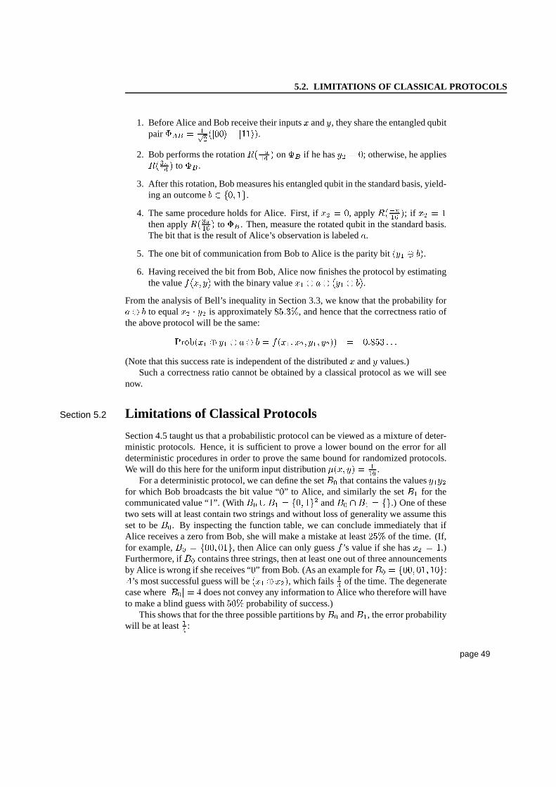
5.2. LIMITATIONS OF CLASSICAL PROTOCOLS

1. Before Alice and Bob receive their inputs� and�, they share the entangled qubitpair�� .

2. Bob performs the rotation�� on�� if he has� � �; otherwise, he applies

�� to ��.

3. After this rotation, Bob measures his entangled qubit in the standard basis, yield-ing an outcome

� � �� .4. The same procedure holds for Alice. First, if� � �

, apply�� ; if � � �then apply�� to ��. Then, measure the rotated qubit in the standard basis.The bit that is the result of Alice’s observation is labeled�.

5. The one bit of communication from Bob to Alice is the paritybit�� .

6. Having received the bit from Bob, Alice now finishes the protocol by estimatingthe value

� �� with the binary value�� .

From the analysis of Bell’s inequality in Section 3.3, we know that the probability for��

to equal� � � is approximately��, and hence that the correctness ratio of

the above protocol will be the same:��

� � � � �� (Note that this success rate is independent of the distributed� and� values.)

Such a correctness ratio cannot be obtained by a classical protocol as we will seenow.

Section 5.2 Limitations of Classical Protocols

Section 4.5 taught us that a probabilistic protocol can be viewed as a mixture of deter-ministic protocols. Hence, it is sufficient to prove a lower bound on the error for alldeterministic procedures in order to prove the same bound for randomized protocols.We will do this here for the uniform input distribution�

�� .For a deterministic protocol, we can define the set�� that contains the values��

for which Bob broadcasts the bit value “�” to Alice, and similarly the set�� for the

communicated value “�”. (With �� and�� .) One of thesetwo sets will at least contain two strings and without loss ofgenerality we assume thisset to be��. By inspecting the function table, we can conclude immediately that ifAlice receives a zero from Bob, she will make a mistake at least �� of the time. (If,for example,�� , then Alice can only guess

�’s value if she has� � �.)

Furthermore, if�� contains three strings, then at least one out of three announcementsby Alice is wrong if she receives “

�” from Bob. (As an example for�� :

�’s most successful guess will be��, which fails �� of the time. The degenerate

case where�� does not convey any information to Alice who therefore will have

to make a blind guess with��

probability of success.)This shows that for the three possible partitions by�� and��, the error probability

will be at least�� :page 49

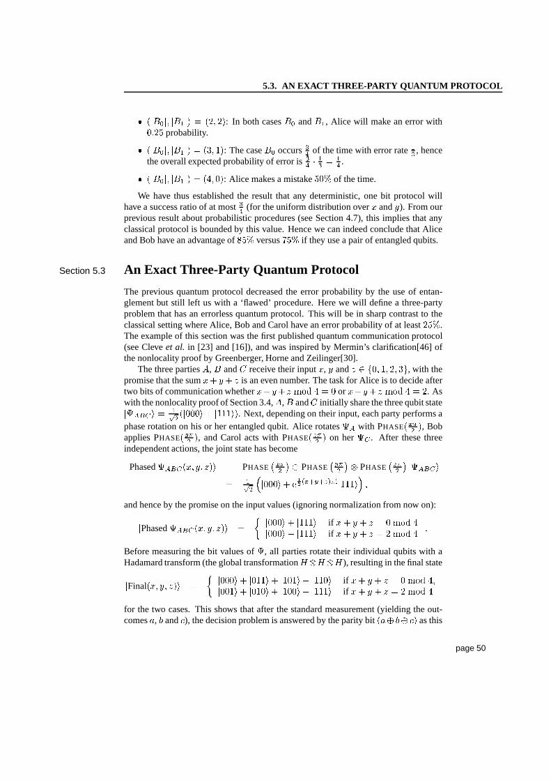
5.3. AN EXACT THREE-PARTY QUANTUM PROTOCOL

�� : In both cases�� and��, Alice will make an error with�� probability.

�� : The case�� occurs

�� of the time with error rate�� , hence

the overall expected probability of error is�� .

�� : Alice makes a mistake

��of the time.

We have thus established the result that any deterministic,one bit protocol willhave a success ratio of at most

�� (for the uniform distribution over� and�). From our

previous result about probabilistic procedures (see Section 4.7), this implies that anyclassical protocol is bounded by this value. Hence we can indeed conclude that Aliceand Bob have an advantage of

��versus

��if they use a pair of entangled qubits.

Section 5.3 An Exact Three-Party Quantum Protocol

The previous quantum protocol decreased the error probability by the use of entan-glement but still left us with a ‘flawed’ procedure. Here we will define a three-partyproblem that has an errorless quantum protocol. This will bein sharp contrast to theclassical setting where Alice, Bob and Carol have an error probability of at least��.The example of this section was the first published quantum communication protocol(see Cleveet al. in [23] and [16]), and was inspired by Mermin’s clarification[46] ofthe nonlocality proof by Greenberger, Horne and Zeilinger[30].

The three parties�, � and� receive their input�, � and� � �� , with thepromise that the sum�� is an even number. The task for Alice is to decide aftertwo bits of communication whether��

or �� . Aswith the nonlocality proof of Section 3.4,�,� and� initially share the three qubit state�� . Next, depending on their input, each party performs aphase rotation on his or her entangled qubit. Alice rotates�� with PHASE

�� , Bobapplies PHASE

�� , and Carol acts with PHASE�� on her��. After these three

independent actions, the joint state has become�Phased��

�� PHASE�� PHASE

�� PHASE��

� ��

and hence by the promise on the input values (ignoring normalization from now on):

�Phased��

�� if � � � � � � � �� if � � � � � � �� Before measuring the bit values of�, all parties rotate their individual qubits with aHadamard transform (the global transformation��), resulting in the final state

�Final

�� if � � � � � � � �� if � � � � � � �� for the two cases. This shows that after the standard measurement (yielding the out-comes�,

�and�), the decision problem is answered by the parity bit

�� as this

page 50

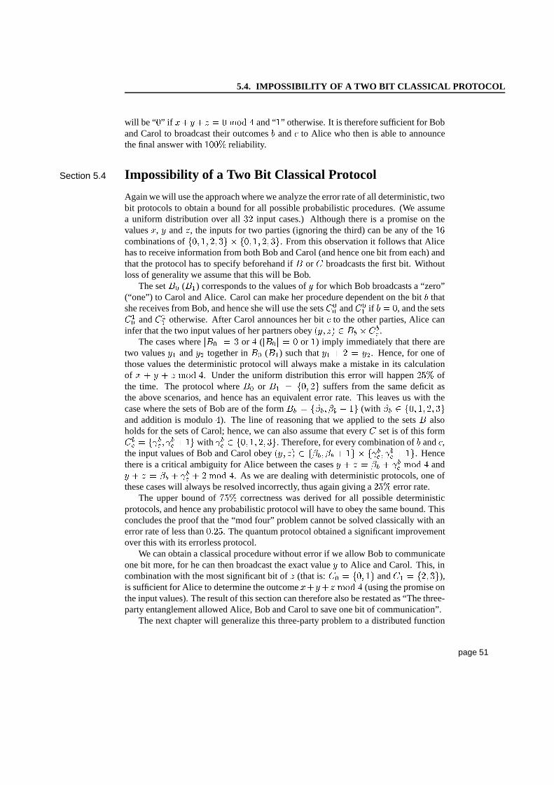
5.4. IMPOSSIBILITY OF A TWO BIT CLASSICAL PROTOCOL

will be “�” if �� and “�” otherwise. It is therefore sufficient for Bob

and Carol to broadcast their outcomes�

and� to Alice who then is able to announcethe final answer with�� reliability.

Section 5.4 Impossibility of a Two Bit Classical Protocol

Again we will use the approach where we analyze the error rateof all deterministic, twobit protocols to obtain a bound for all possible probabilistic procedures. (We assumea uniform distribution over all

�� input cases.) Although there is a promise on thevalues�, � and�, the inputs for two parties (ignoring the third) can be any ofthe ��combinations of�� . From this observation it follows that Alicehas to receive information from both Bob and Carol (and henceone bit from each) andthat the protocol has to specify beforehand if� or � broadcasts the first bit. Withoutloss of generality we assume that this will be Bob.

The set�� (��) corresponds to the values of� for which Bob broadcasts a “zero”(“one”) to Carol and Alice. Carol can make her procedure dependent on the bit

�that

she receives from Bob, and hence she will use the sets�� and�� if� � �

, and the sets�� and�� otherwise. After Carol announces her bit� to the other parties, Alice caninfer that the two input values of her partners obey

��

�.

The cases where��

or � (��

or �) imply immediately that there aretwo values�� and� together in�� (��) such that�� . Hence, for one ofthose values the deterministic protocol will always make a mistake in its calculationof � � � � � �� . Under the uniform distribution this error will happen�� ofthe time. The protocol where�� or �� suffers from the same deficit asthe above scenarios, and hence has an equivalent error rate.This leaves us with thecase where the sets of Bob are of the form��

�� (with �� and addition is modulo�). The line of reasoning that we applied to the sets� alsoholds for the sets of Carol; hence, we can also assume that every � set is of this form��

��

��

�� with ��

�� . Therefore, for every combination of

�and�,

the input values of Bob and Carol obey��

��

��

�� . Hence

there is a critical ambiguity for Alice between the cases� � � � ��

�� and� � � � ��

�� . As we are dealing with deterministic protocols, one of

these cases will always be resolved incorrectly, thus againgiving a�� error rate.The upper bound of

��correctness was derived for all possible deterministic

protocols, and hence any probabilistic protocol will have to obey the same bound. Thisconcludes the proof that the “mod four” problem cannot be solved classically with anerror rate of less than

��. The quantum protocol obtained a significant improvementover this with its errorless protocol.

We can obtain a classical procedure without error if we allowBob to communicateone bit more, for he can then broadcast the exact value� to Alice and Carol. This, incombination with the most significant bit of� (that is:�� and�� ),is sufficient for Alice to determine the outcome�� (using the promise onthe input values). The result of this section can therefore also be restated as “The three-party entanglement allowed Alice, Bob and Carol to save one bit of communication”.

The next chapter will generalize this three-party problem to a distributed function

page 51

5.4. IMPOSSIBILITY OF A TWO BIT CLASSICAL PROTOCOL

for � parties. This will give us an unbounded difference in terms of communicationcomplexity between the quantum and the classical settings.

page 52

Chapter 6

Multiparty QuantumCommunication Complexity

The three-party problem of the previous chapter can be generalized to a� party dis-tributed computation. In this chapter we will show how this leads to a quantum proto-col that gives a reliable answer after only� � �bits of communication, whereas in theclassical setting the parties would require of the order of� �� bits. This result waspublished in the October 1999 issue ofPhysical Review Aunder the title “MultipartyQuantum Communication Complexity”, with co-authors HarryBuhrman, Peter Høyerand Alain Tapp.[19]

Section 6.1 Multiparty Problem and Its Quantum Complexity

In the � party scenario, every participant�� receives a real number�� , withthe joint promise that the total sum�� is a natural number. The task for Alice (��)is to determine whether this sum is an even or an odd number: the calculation of thefunction value

Odd?��

�� Our first result will be that if the parties share a� qubit entangled state, this problemcan be solved with a protocol where each party communicates only one bit to Alice.This is shown by the following procedure which therefore hasa total communicationcomplexity of� � �bits.

Section 6.2 The Quantum Protocol

Let the parties�� initially share the entangled state��

page 53

6.3. BOUNDS FOR PROMISE FUNCTIONS

where each party�� possesses the qubit��. Depending on their input value��, a phaserotation PHASE

�� is applied to this qubit��. Just as for the three-party scenario,this leads to essentially two different possibilities (ignoring normalization)

�Phased�� PHASE

�� PHASE��

��

�� if �� is even,

�� if �� is odd.

Hence, locally applying the Hadamard transform on all� sites results in a superposi-tion of bit strings with an even (odd) Hamming weight, if the summation�� equalsan even (odd) number. The continuation of the protocol should now be obvious: everyparty measures his or her qubit�� in the standard basis and (except Alice) broadcaststhe outcome�� to��. She concludes by calculating the total parity�� of themeasurement outcomes, which directly gives the correct answer to the original ques-tion: “Is �� even or odd?” A protocol with less than� � � bits of communicationis impossible as this implies the exclusion of one of the parties, which cannot give anerrorless procedure.

The core of this chapter is the proof that in the classical case, �� bits ofcommunication are required. This is far from trivial, as we will see in the next sections:a case-by-case analysis (as we did in the three-party case) is no longer possible.

Section 6.3 Bounds for Promise Functions

In the introductory chapter, “Communication Complexity”,we discussed how a deter-ministic communication protocol corresponds to a tree where the leaves label the finaldecisions, and the depth of the tree equals the communication complexity of the pro-tocol. What follows is a general method for obtaining lower bounds on deterministicprotocols that we will use in the next section for our “even versus odd” problem.

First we remind ourselves that a protocol has to be well defined for all inputs�� , even if they do not obey the promise of the function�

�� .This means that for every instance�� , the protocol has to follow one uniquelydetermined path from the root to a ‘decision leaf’. Because our tree is binary, thisimplies that with depth�, the number of leaves is at most��. Hence, if we have aminimum of � leaves, then this corresponds to a communication complexity of at least“depth��” � �� bits. This gives us a good reason to look at the number ofleaves that is required for a deterministic and exact protocol.

For different input combinations, a protocol can end up in the same decision leaf.Assume now that we know of two such combinations

�� and��

that both lead to the same ‘path down the decision tree’ to a leaf�. For a given protocol,the direction that the protocol takes at a specific branch is solely determined by theinput of the then speaking party��. Note now that by our assumption, these directionsare the same for both�� and ��. This means that we can combine the� and �� valuesand still take the same path down to�. In other words, every element of the Cartesian

page 54

6.4. THE LOWER BOUND FOR THE CLASSICAL PROTOCOL

product set�� gives the same path down the tree. We will

therefore call the subset of inputs that lead to the same leaf arectangle,as they willalways be of the form �� , with �� for every

�.

If we want our deterministic protocol to be exact, then the elements of a specificrectangle that are allowed by the promise must all have the same function value

�.

We can assume that every leaf contains at least one allowed input for it would otherwisebe possible to ‘trim down’ the decision tree—by removing this vacuous leaf—withoutchanging the effectiveness of the protocol. These two characteristics are summarizedby saying that the rectangles have to bemonochromatic.

We thus have collected some facts about the leaves of a decision tree that we can usein the following standard method for proving bounds on deterministic communicationprotocols. (See also Section 1.2 in [42].)

Assume a (promise)�-party decision problem�

�� where there isa total of

�� possible input states (both proper and improper in the case of promiseproblems).

1. Show that for the function�

the maximum volume for a monochromatic rectangleis bounded by some limit�.

2. Realize that this bound tells us that there have to be at least�� ‘rectangles-as-

leaves’ in the decision tree.

3. Conclude that a deterministic protocol will therefore needat least� �� bits of communication if it wants to be errorless.

This is the approach that we will now apply to our “Odd?” function.

Section 6.4 The Lower Bound for the Classical Protocol

Before we start our lower bound proof, we will rephrase and restrict the Odd?-problemto the ‘finite and integer input’ version that we already encountered in Section 5.3.This is the situation where we are only interested in values of � up to� bits and wherewe (implicitly) multiply every number with�� such that every�� is viewed as anelement of

��. We therefore have the new promise that�� , forwhich the parties try to determine whether

� �� (“even”), or

�� (“odd”)?

It should be clear that the original Odd?-function isat leastas difficult to solve as thisproblem: as� gets bigger the problem becomes harder and only the limitingcase� �� corresponds to the continuous version with� � �� rather than� � � �� . It turns out however, that for our current purposes the lower bound� �� suffices (in combination with� �). We will now prove the�� lower boundfor this restricted problem.

Let be a�-dimensional rectangle that corresponds to a leaf in the decision tree,hence � � � � � � �� . With modulo�� arithmetic, we define the sum of

page 55

6.4. THE LOWER BOUND FOR THE CLASSICAL PROTOCOL

two sets�� as� � � � ��

. We use this set additionand the ‘sides’�� to define a sequence of� � � sets

�� by:�� and�� for

� � �� . Obviously, for every combination�� in therectangle, the corresponding value�� is an element of

�� . The

requirement that is monochromatic tells us thateither� � �

� or �� , but not

both. This puts a bound on the size of�� and hence on the volume of the rectangle

as we will see with the help of some group theory.Assume without loss of generality that is a zero-rectangle, and hence that

� � ��

and�� . one: � � ��. Now we are at the place where we have to use an

application ofKneser’s addition theoremfor groups[39, 43], which states:

For every pair of subsets�� there exists a subgroup� of��

such that�� and��

��.

We apply this theorem to the cases where� � �� and� � � (and hence��

� �� with� � �� ), which gives us� groups�� that obey

��

� �� This readily shows that for every

�the only possible�� is the trivial subgroup��

��, for if �� is a bigger subgroup, then�� and

�� would not

correspond to a monochromatic rectangle (remember that� � �

�). By the second partof Kneser’s theorem we therefore know that

�� for all�, which

sums up to

��

�� The exclusion of the element�� for the set

�� gives us

�� , leading to

� ��

for the sides of the rectangle, and hence for its maximum volume�

� � � ��

��

�� The last equation shows us an upper bound� on a monochromatic rectangle for an

exact�-party solution to the Odd?-problem (with input size�). The decision tree ofthis protocol has to cover a total of�� inputs and hence needs at least

�� leaves. This

gives the tree a minimum depth of� �� , by the assumptions� �� and� �.The method of the previous section now concludes our proof that every classical

and exact� party protocol for the Odd?-function requires at least� �� bits of communication.

page 56

6.5. CONCLUSION

Section 6.5 Conclusion

We just saw a difference between classical and quantum communication of the order of� �� for � parties. This assures us that the quantum protocol is more efficienteven ifwe want to take into account the distribution of the entangled qubitsduring the initialstage of the protocol. If the cost of transmitting�qubit equals� classical bits, then thequantum complexity still remains linear in�. For large enough� (i.e. ��

)the resources that the classical procedure requires are still more than the costs

�� in the quantum scenario.

page 57

Chapter 7

Quantum Whispers

Probabilities in quantum mechanics depend quadratically on the amplitudes of a state.This phenomenon lies at the heart of the so called ‘quantum Zeno effect’. In thischapter, we will use this effect to establish a difference between classical and quantumcommunication in the probabilistic model. We will show how the error probability ofthe one-bit quantum protocol will always be lower than that of the classical approach.This result is extended to the setting where each party, in a sequence of many parties,is only allowed to communicate one bit to its neighbor (akin to the game of ‘ChineseWhispering’). It is argued that for this multiparty problem, there is no reliable classicalsolution, whereas with entanglement it can be solved easily. The results of this chapterwere published in the article “Quantum communication usinga nonlocal Zeno effect”by Lucien Hardy and myself.[34]


In this chapter, we will employ the ‘quantum Zeno effect’ to construct a new quantumcommunication procedure. This effect relies on the quadratic, rather than linear, rela-tion between the amplitudes and the probabilities of a quantum state. Several authorshave used this phenomenon to obtain proofs of nonlocality that are different from theones that we encountered in the previous chapters of this thesis.[15, 33, 62]

First, we will define a two-party problem Jump?�� for which prior entanglement

enables us to significantly reduce the error over the classical scenario. After that, amultiparty version, “Quantum Whispers”, of the same problem is introduced. For thistask we exhibit a reliable quantum protocol and argue that without entanglement nosuch solution exists.

Section 7.2 The Two-Party Problem

The “jump or no jump?” question that we will discuss in this chapter is a typicalexample of a promise problem. In the two-party setting Aliceand Bob receive their

page 58

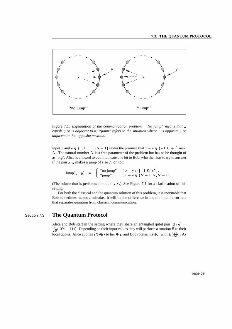
7.3. THE QUANTUM PROTOCOL

‘‘no jump’’ ‘‘jump’’

x x

yy

Figure 7.1: Explanation of the communication problem. “No jump” means that �equals� or is adjacent to it; “jump” refers to the situation where� is opposite� oradjacent to that opposite position.

input� and� � �� under the promise that� �� . The natural number� is a free parameter of the problem but has to be thought ofas ‘big’. Alice is allowed to communicate one bit to Bob, who then has to try to answerif the pair�� makes a jump of size� or not:

Jump?�� “no jump” if � � � � ��,

“jump” if � � � � �� .(The subtraction is performed modulo��.) See Figure 7.1 for a clarification of thissetting.

For both the classical and the quantum solution of this problem, it is inevitable thatBob sometimes makes a mistake. It will be the difference in the minimum error ratethat separates quantum from classical communication.

Section 7.3 The Quantum Protocol

Alice and Bob start in the setting where they share an entangled qubit pair�� . Depending on their input values they will perform a rotation to their

local qubits. Alice applies�� to her��, and Bob rotates his�� with � �� . As

page 59

7.3. THE QUANTUM PROTOCOL

a result of these two actions, the joint state is now of the form

��

��

��

After the rotations, when both parties measure their qubit in the standard basis, theparity of the two outcomes� and

�is strongly correlated with the difference between�

and�:

��

By the periodicity of the trigonometric functions, the parity�� will give a reliable

indication of the “jump versus no jump” question. In the casewhere� and� do notmake a jump, we have

��

and hence

�� no jump between� and��

�� no jump between� and��

Conversely, in the case where there is a jump between� and� we have

��

and consequently

�� jump between� and��

jump between� and��

The above analysis suggests the protocol where Alice sends her measurement out-come� to Bob, who then calculates the parity

�� . By doing so, the error rate of

Bob’s estimation will be bounded by the quadratic expression

��

Next, we will show that anyclassicalprotocol will have a error probability of theorder

�� .

page 60

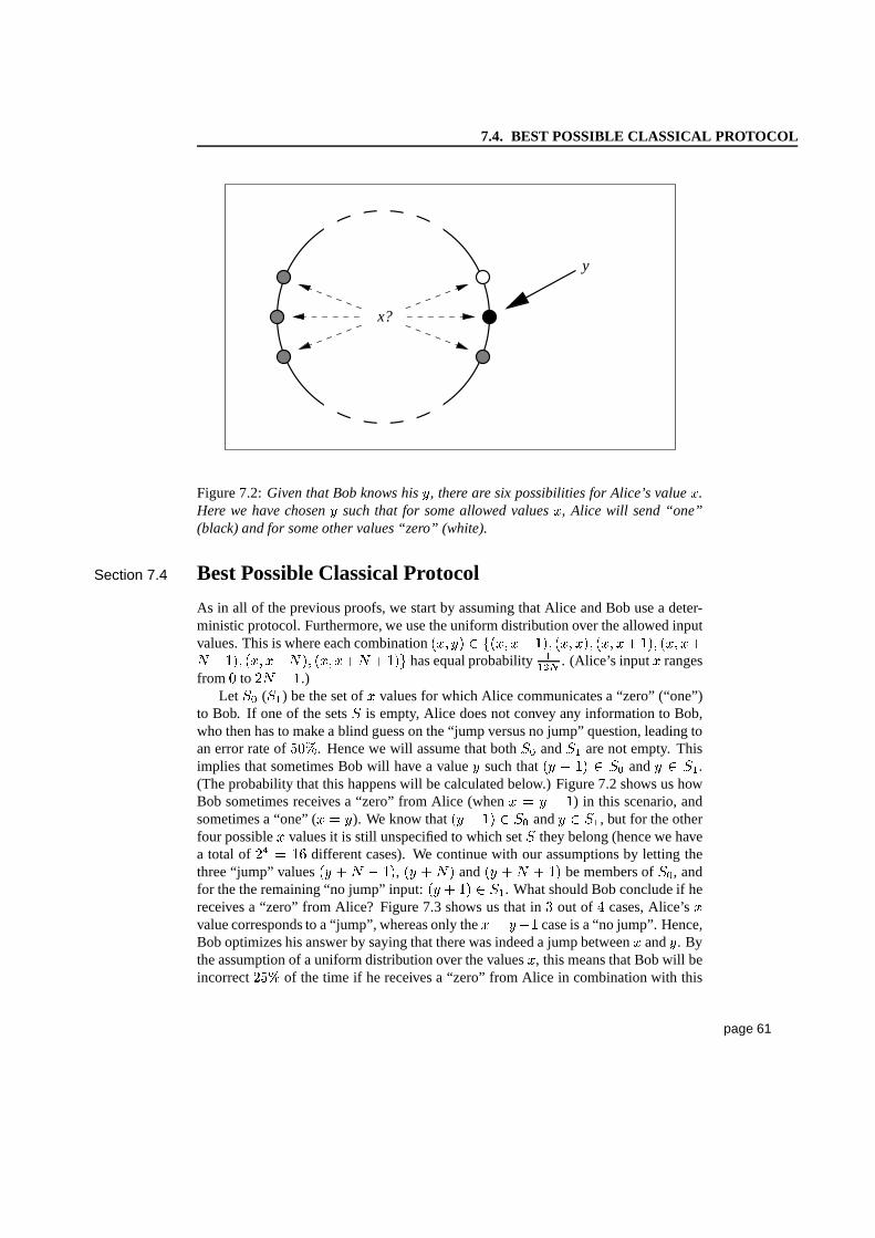
7.4. BEST POSSIBLE CLASSICAL PROTOCOL

y

x?

Figure 7.2:Given that Bob knows his�, there are six possibilities for Alice’s value�.Here we have chosen� such that for some allowed values�, Alice will send “one”(black) and for some other values “zero” (white).

Section 7.4 Best Possible Classical Protocol

As in all of the previous proofs, we start by assuming that Alice and Bob use a deter-ministic protocol. Furthermore, we use the uniform distribution over the allowed inputvalues. This is where each combination

�� has equal probability �� . (Alice’s input� rangesfrom

�to �� .)

Let�� (

��) be the set of� values for which Alice communicates a “zero” (“one”)to Bob. If one of the sets

�is empty, Alice does not convey any information to Bob,

who then has to make a blind guess on the “jump versus no jump” question, leading toan error rate of

��. Hence we will assume that both

�� and�� are not empty. This

implies that sometimes Bob will have a value� such that�� and� � ��.

(The probability that this happens will be calculated below.) Figure 7.2 shows us howBob sometimes receives a “zero” from Alice (when� � � � �) in this scenario, andsometimes a “one” (� � �). We know that

�� and� � ��, but for the otherfour possible� values it is still unspecified to which set

�they belong (hence we have

a total of�� different cases). We continue with our assumptions by letting thethree “jump” values

�� , �� and�� be members of

��, andfor the the remaining “no jump” input:

�� . What should Bob conclude if hereceives a “zero” from Alice? Figure 7.3 shows us that in

�out of � cases, Alice’s�

value corresponds to a “jump”, whereas only the� � ��case is a “no jump”. Hence,Bob optimizes his answer by saying that there was indeed a jump between� and�. Bythe assumption of a uniform distribution over the values�, this means that Bob will beincorrect�� of the time if he receives a “zero” from Alice in combination with this

page 61

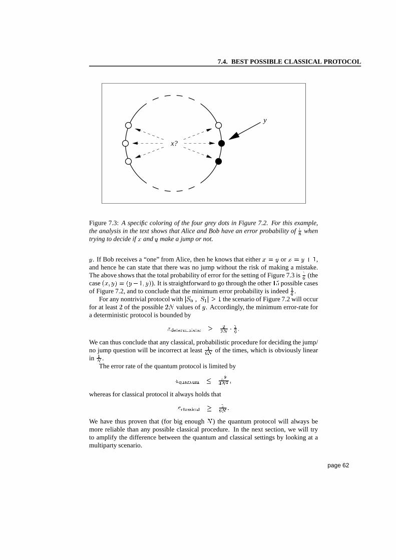
7.4. BEST POSSIBLE CLASSICAL PROTOCOL

y

x?

Figure 7.3:A specific coloring of the four grey dots in Figure 7.2. For this example,the analysis in the text shows that Alice and Bob have an errorprobability of �� whentrying to decide if� and� make a jump or not.

�. If Bob receives a “one” from Alice, then he knows that either� � � or � � � � �,and hence he can state that there was no jump without the risk of making a mistake.The above shows that the total probability of error for the setting of Figure 7.3 is�� (thecase

�� ). It is straightforward to go through the other��possible casesof Figure 7.2, and to conclude that the minimum error probability is indeed �� .

For any nontrivial protocol with�� , �� the scenario of Figure 7.2 will occur

for at least� of the possible�� values of�. Accordingly, the minimum error-rate fora deterministic protocol is bounded by

�� We can thus conclude that any classical, probabilistic procedure for deciding the jump/no jump question will be incorrect at least�� of the times, which is obviously linearin �� .The error rate of the quantum protocol is limited by

��

whereas for classical protocol it always holds that

�� We have thus proven that (for big enough�) the quantum protocol will always bemore reliable than any possible classical procedure. In thenext section, we will tryto amplify the difference between the quantum and classicalsettings by looking at amultiparty scenario.

page 62

7.5. MULTIPARTY COMMUNICATION PROBLEM

Section 7.5 Multiparty Communication Problem

Imagine the above two-party problem as the first step of a multiparty problem. In thisscenario we consider a concatenation of jump/no jump questions for a line-up ofparties that are only allowed to communicate one bit to theirnext neighbor. This settingis reminiscent of the game “Chinese Whispers”, where a message passes through a rowof whispering people. Hence the name “Quantum Whispers”.

Formally the problem is defined as follows. Take parties�� , each havetwo input values

�� except for the first party who only receives an��, and the lastperson�� with his �

�. The promise on the input is the same that we used for thejump versus no jump problem:

��

for all � � � (note that�� and�� are uncorrelated). After having received theirrespective inputs, each party�� is allowed to communicate one bit�� to his or herneighbor��. After these � � bits of communication, the rightmost participant�� has to decide whether there was an even or an odd number of jumps among the � �pairs

�� .We are interested in the error rate in the case where is of the same order as�

(that is, � �� with � � ��. The quantum solution to the quantum whispersproblem will be a straightforward application of the two-party procedure for each cou-ple

�� . For big enough�, this will give us a reliable quantum protocol. Wethen continue by arguing that in the classical setting such areliable protocol does notexist. But it should be stressed that a formal proof of this claim is still lacking.

Section 7.6 The Quantum Whispers Protocol

Before receiving their input values, each pair�� shares an entangled state�� . (This notation as to distinguish the qubit�� that is en-

tangled with the system of�� from �� that is correlated with the qubit�� of��.)

The first two parties start by performing the same rotations,on their respectivequbits�� and�, as was described in the section on the two-party setting.

The standard measurement on both sides yields the classicalbits �� and� (of

which �� will be sent to� by the first party). From earlier investigations, we knowthat the parity

�� indicates with�� certainty whether or not there is a jump

between�� and�.These rotations and measurements are done by all � � couples

�� ontheir qubits�� and�� (the rotations depending on the respective input values��and��). The estimations of the jump/no jump answers are the classical parity bits�� , and hence the question “is there an even or odd number of jumps?” can be

estimated by the total parity�� . Therefore, after�� has sent her�� to

her neighbor,� continues by communicating the bit�� to the third person

in line. This procedure of sending the parity of the receivedbit and the two outcomes

page 63

7.7. ERROR OF THE QUANTUM WHISPERS PROTOCOL

�� and�� to �� is repeated until�� is reached. The bit that this rightmost party

receives from�� corresponds to the previously mentioned sum�� ,minus his own outcome

��. Hence, by taking the parity of the received bit and

��,

he will effectively estimate the odd/even jumps questions by � � repetitions of thetwo-party protocol. This allows an easy analysis of the expected error, as we will seebelow.

Section 7.7 Error of the Quantum Whispers Protocol

In the description of the quantum whispers approach to solving the odd/even jumpsproblem, it was mentioned how it is equivalent with � � applications of the two-party solution. We know that the error rate of this procedureis bounded from aboveby �� . Hence, the probability of success� � �� of the multiparty protocol isthe sum of the probabilities corresponding to an even numberof mistakes among the � �guesses. The lower bound on this probability is calculated by

��

��

� � � ��

�� For some constant� � �

� and a large enough�, this can be approximated by onlyconsidering the

� �case; it hence has a success probability of at least

��

��

This shows that the � �� party version of the quantum whispers protocol has amaximum error rate of the order

�� . In the case of large�, this yields a reliable

quantum protocol.

Section 7.8 Possible Classical Whispers

Here we will argue that there does not exist a reliable classical protocol for the even/oddjumps problem (again for large� and� � �

� � ��).We start by noting that the “jump” versus “no jump” problem isindependent for

each�� pair because there is no correlation between�� and��. The parity of

the number of jumps relies critically on all the��answers to the two-party problemwhich are independent of each other. This strongly suggeststhat it is necessary to solvethe jump/no jump problem for all pairs

�� . Because we only allow a single bitof communication between the parties�� and��, this will always induce an error-rate of at least �� per pair. (See the result of Section 7.4.) With the number of pairs � � � �� , the probability of an odd number of such errors (leading to an

page 64

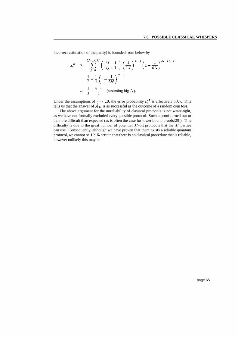
7.8. POSSIBLE CLASSICAL WHISPERS

incorrect estimation of the parity) is bounded from below by

��

� � � � � ��

��

��

� ��

��

� ��

��

� (assuming big�) �Under the assumptions of� � ��, the error probability�� is effectively

��. This

tells us that the answer of�� is as successful as the outcome of a random coin toss.The above argument for the unreliability of classical protocols is not water-tight,

as we have not formally excluded every possible protocol. Such a proof turned out tobe more difficult than expected (as is often the case for lowerbound proofs[29]). Thisdifficulty is due to the great number of potential-bit protocols that the partiescan use. Consequently, although we have proven that there exists a reliable quantumprotocol, we cannot be��certain that there is no classical procedure that is reliable,however unlikely this may be.

page 65

Chapter 8

Lower Bounds for QuantumCommunication

In the previous chapters, we have only seen examples where entanglement reduced thecomplexity of communication protocols. Here we give our first lower bound for quan-tum communication. We will show that for the inner product problem, entanglementdoes not significantly improve the performance over the classical case. The quantumand classical scenario are nevertheless not equivalent. This difference is indicated by asmall reduction of error in the� � � case of the inner product problem with only onebit of communication between the parties. See [24] for the original article by RichardCleve, Alain Tapp, Michael Nielsen and myself.


How can we prove lower bounds for quantum communication? Obviously, some ofthe methods we use for classical communication fail; otherwise there would be nodifference between the two. Hence, we have to look for ‘impossibilities in quantummechanics’ and try to apply them in the setting of distributed computation. The prob-lem is that, at the moment, we do not have many examples of tasks that are impossiblein a nonlocal world. Instead, our path to understanding entanglement is paved with un-expected phenomena that do not exist in classical information theory. One of the few‘no-go’s’ in quantum communication is Holevo’s bound, which tells us that quantumbits are not any better than classical ones for transferringinformation between parties.This bound, in combination with a result by Michael Nielsen (see Appendix A), willindeed be one of the cornerstones for this chapter’s lower bound.

The crucial step in the proof that will follow is to go from theproblem that onlyfocuses on the single bit of the function

� �� to the transfer of the whole bit string�. This is done by considering an�

that is familiar both in communication complexityand in quantum computation: the inner product function.

page 66

8.2. THE INNER PRODUCT PROBLEM

Section 8.2 The Inner Product Problem

For two parties� and� with input strings�� and

�� , the innerproduct function

�� is defined by

��

��

This function is well studied as a classical communication problem. (See [20, 64]and Section 3.5 in [42].) It is easy to see that for a deterministic protocol,� bitsof communication are required. This intractability of

��does not disappear in the

probabilistic scenario. If Alice and Bob want to know�� with a maximum error

of �, then� � �� bits of communication are still necessary. Hence for afixed error rate, the communication complexity is� � ��. Below we will see thatboth for the deterministic and probabilistic cases, the situation does not much improveif the two parties are allowed to use prior entanglement. That is, the inner productfunction is also hard in the setting of quantum communication.

In quantum computation, the��

function is inextricably linked with the Hadamardtransform. This was already mentioned in the section on quantum information, but wewill briefly repeat it here. The one qubit Hadamard transform� is defined by

� �� and � �� which also shows that� is its own inverse:�

� �.When we apply a Hadamard to each individual bit of the string� � �� , we

obtain a superposition of all possible� bit strings� where the information about� isstored in the phases as the inner product between� and the different�’s:

��

��

�� (8.1)

This suggests the following protocol to extract� bits of information�� withthe help of the inner product function

��. We start with the uniform superpositionof all strings� � �� and an empty output register:

��

��Calculating the function values

�� in superposition then yields

��

��We now apply a conditional phase flip (CFLIP) on the output register,

��

��

��

page 67

8.3. INFORMAL SKETCH OF PROOF

after which we inverse the first computation of the function value, thereby giving thefinal state

��

��

�� Equation 8.1 shows us that this last state gives us all the� bits of the string�.

We thus see how the quantum calculation of the inner product for a superpositionof � strings results in a protocol where we obtain� bits of information. We will usethis phenomenon in combination with the known quantum limitations on informationtransfer to prove our lower bounds on the quantum communication complexity of the��

function.

Section 8.3 Informal Sketch of Proof

Before we write down the formal proof of the quantum lower bounds, we will first givean overview of the ideas that lie behind it. Assume that Aliceand Bob can compute theinner product value

�� of their� bit strings with� classical bits of communica-tion. Instead of classical inputs, let Alice use the superposition of all possible strings� while Bob fixes his�. The two parties then continue by executing the protocol ‘inquantum parallel’ that now uses� quantum bits of communication. Having finishedthis procedure, Alice now has a superposition of strings� entangled with the�� func-tion values

��. As we saw in the previous section, this information can easily beconverted into a description of Bob’s� bits �� . Hence Alice has—with� qubitsof communication—obtained� bits of information. The bounds on quantum informa-tion transfer tell us that this is only possible if� � � , which is tight by the method ofSuperdense coding (see Section 2.3).

For the probabilistic bound, we use the same argument by saying: “ � � � the ��function valuesapproximating

�� into a descriptionstrongly correlatedwith� � � � only possible if� is of the order of�.”Our main concern for the formal proof will be the conversion of the protocol for

classical inputs into its quantum superposition variant. This reduction provides a newmethod of analysis that can also be used for other, future lower bounds in quantumcommunication. The formal justification of it will be given in the next section.

Section 8.4 Quantum Parallelizing Communication Protocols

Let Alice and Bob share some initial entanglement�� before they receive their inputs� and�. During the execution of the communication protocol, the two parties will mostlikely need some additional ‘working space’ to perform the appropriate computations,after which Alice writes down the outcome

� ��. Without loss of generality, weassume these ancillas to be initially set to zero, and hence the whole system starts inthe state

�begin

�� page 68

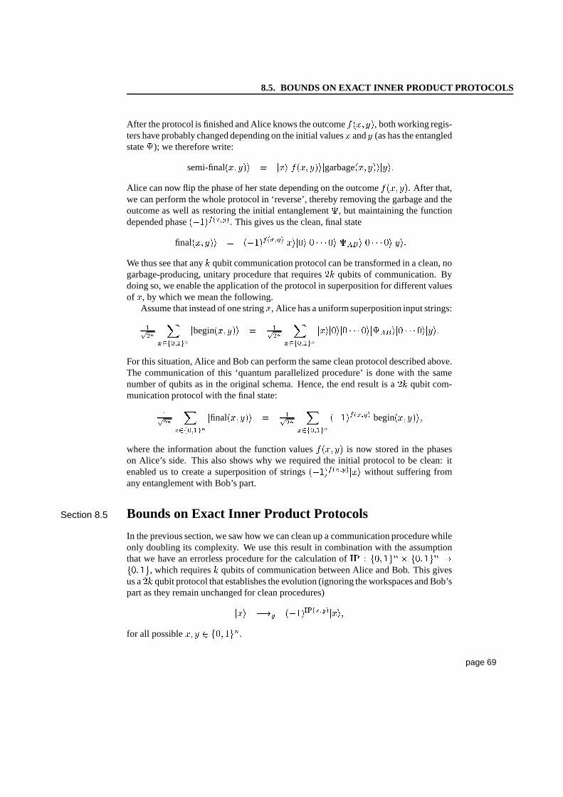
8.5. BOUNDS ON EXACT INNER PRODUCT PROTOCOLS

After the protocol is finished and Alice knows the outcome� ��, both working regis-

ters have probably changed depending on the initial values� and� (as has the entangledstate�); we therefore write:

�semi-final

�� garbage��

Alice can now flip the phase of her state depending on the outcome� ��. After that,

we can perform the whole protocol in ‘reverse’, thereby removing the garbage and theoutcome as well as restoring the initial entanglement�, but maintaining the functiondepended phase

�� . This gives us the clean, final state

�final

��

We thus see that any� qubit communication protocol can be transformed in a clean,nogarbage-producing, unitary procedure that requires�� qubits of communication. Bydoing so, we enable the application of the protocol in superposition for different valuesof �, by which we mean the following.

Assume that instead of one string�, Alice has a uniform superposition input strings:

��

�begin

��

�� For this situation, Alice and Bob can perform the same clean protocol described above.The communication of this ‘quantum parallelized procedure’ is done with the samenumber of qubits as in the original schema. Hence, the end result is a �� qubit com-munication protocol with the final state:

��

�final

��

�� begin

��

where the information about the function values� �� is now stored in the phases

on Alice’s side. This also shows why we required the initial protocol to be clean: itenabled us to create a superposition of strings

�� without suffering from

any entanglement with Bob’s part.

Section 8.5 Bounds on Exact Inner Product Protocols

In the previous section, we saw how we can clean up a communication procedure whileonly doubling its complexity. We use this result in combination with the assumptionthat we have an errorless procedure for the calculation of

��

�� , which requires� qubits of communication between Alice and Bob. This givesus a�� qubit protocol that establishes the evolution (ignoring the workspaces and Bob’spart as they remain unchanged for clean procedures)

��

��

for all possible�� .

page 69

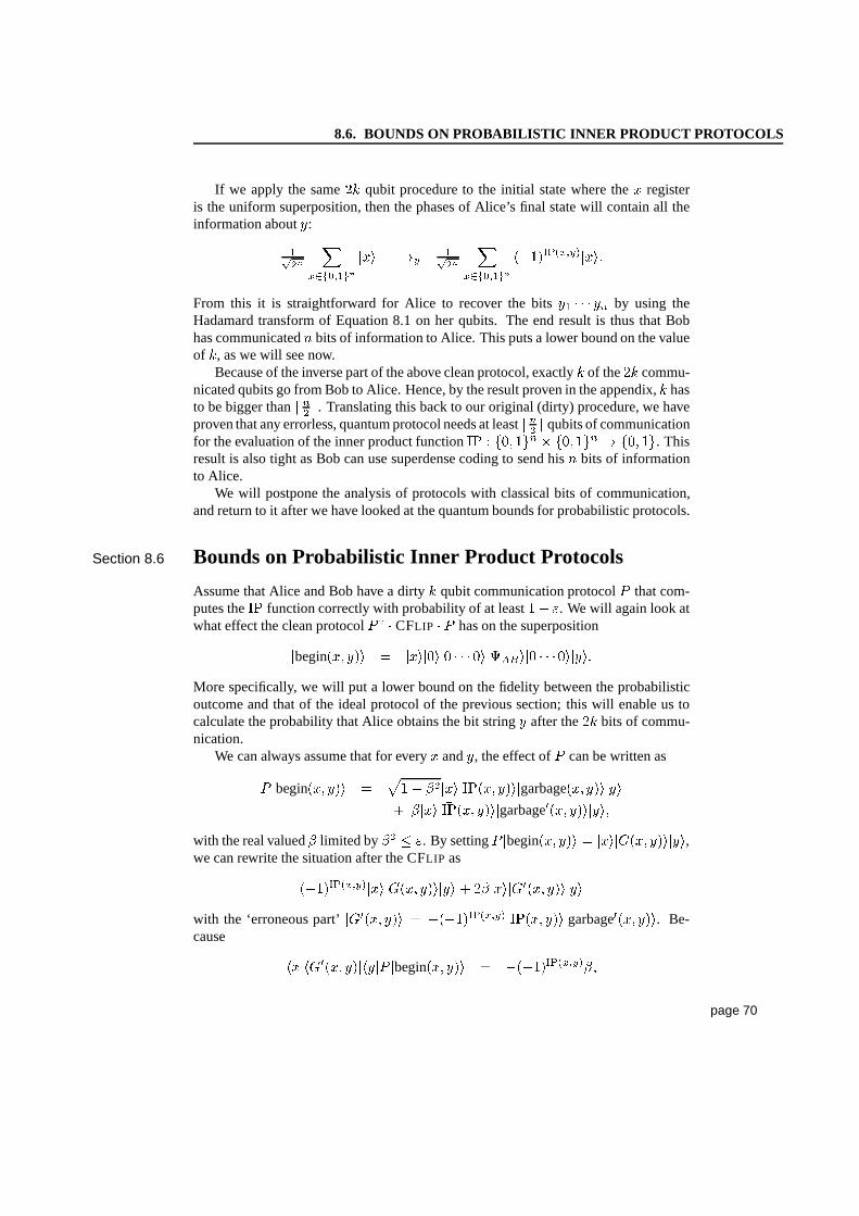
8.6. BOUNDS ON PROBABILISTIC INNER PRODUCT PROTOCOLS

If we apply the same�� qubit procedure to the initial state where the� registeris the uniform superposition, then the phases of Alice’s final state will contain all theinformation about�:

��

��

��

�� From this it is straightforward for Alice to recover the bits�� by using theHadamard transform of Equation 8.1 on her qubits. The end result is thus that Bobhas communicated� bits of information to Alice. This puts a lower bound on the valueof �, as we will see now.

Because of the inverse part of the above clean protocol, exactly � of the�� commu-nicated qubits go from Bob to Alice. Hence, by the result proven in the appendix,� hasto be bigger than�� . Translating this back to our original (dirty) procedure, we haveproven that any errorless, quantum protocol needs at least�� qubits of communicationfor the evaluation of the inner product function

�� . This

result is also tight as Bob can use superdense coding to send his � bits of informationto Alice.

We will postpone the analysis of protocols with classical bits of communication,and return to it after we have looked at the quantum bounds forprobabilistic protocols.

Section 8.6 Bounds on Probabilistic Inner Product Protocols

Assume that Alice and Bob have a dirty� qubit communication protocol�

that com-putes the

��function correctly with probability of at least��. We will again look at

what effect the clean protocol� � �CFLIP �� has on the superposition

�begin

�� More specifically, we will put a lower bound on the fidelity between the probabilisticoutcome and that of the ideal protocol of the previous section; this will enable us tocalculate the probability that Alice obtains the bit string� after the�� bits of commu-nication.

We can always assume that for every� and�, the effect of�

can be written as� �begin

�� garbage

�� garbage�

��with the real valued� limited by� � �. By setting

� �begin

�� ,we can rewrite the situation after the CFLIP as

��

with the ‘erroneous part’��

�� garbage�

��. Be-cause

�� begin

��

��

page 70

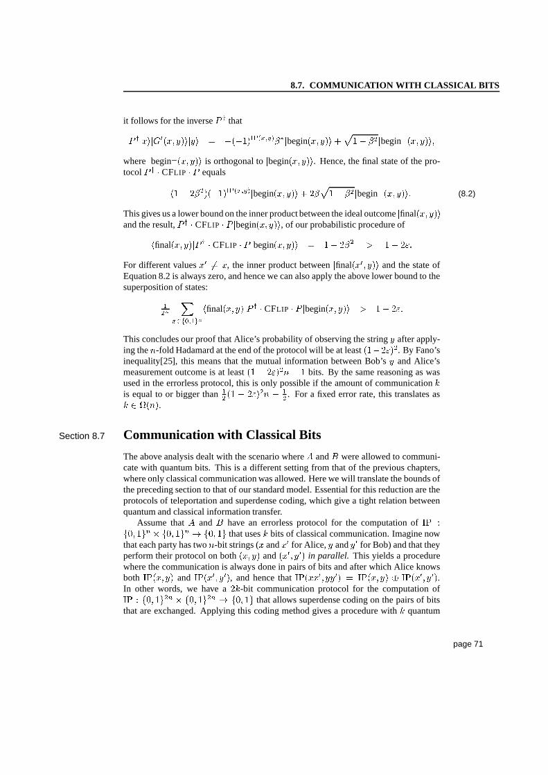
8.7. COMMUNICATION WITH CLASSICAL BITS

it follows for the inverse� �

that� � ��

�� begin�� begin�

��where

�begin�

�� is orthogonal to�begin

��. Hence, the final state of the pro-tocol

� � �CFLIP �� equals

�� begin�� begin�

�� (8.2)

This gives us a lower bound on the inner product between the ideal outcome�final

��and the result,

� � �CFLIP �� begin

��, of our probabilistic procedure of

�final

�� CFLIP �� begin

�� For different values�� , the inner product between

�final

�� and the state ofEquation 8.2 is always zero, and hence we can also apply the above lower bound to thesuperposition of states:

��

�final

�� CFLIP �� begin

�� This concludes our proof that Alice’s probability of observing the string� after apply-ing the�-fold Hadamard at the end of the protocol will be at least

��. By Fano’sinequality[25], this means that the mutual information between Bob’s� and Alice’smeasurement outcome is at least

�� bits. By the same reasoning as wasused in the errorless protocol, this is only possible if the amount of communication�is equal to or bigger than� �� . For a fixed error rate, this translates as� � ��.

Section 8.7 Communication with Classical Bits

The above analysis dealt with the scenario where� and� were allowed to communi-cate with quantum bits. This is a different setting from thatof the previous chapters,where only classical communication was allowed. Here we will translate the bounds ofthe preceding section to that of our standard model. Essential for this reduction are theprotocols of teleportation and superdense coding, which give a tight relation betweenquantum and classical information transfer.

Assume that� and � have an errorless protocol for the computation of��

�

�� that uses� bits of classical communication. Imagine nowthat each party has two�-bit strings (� and�� for Alice, � and�� for Bob) and that theyperform their protocol on both

�� and�� in parallel. This yields a procedure

where the communication is always done in pairs of bits and after which Alice knowsboth

�� and�� , and hence that

�� .In other words, we have a��-bit communication protocol for the computation of��

� �� that allows superdense coding on the pairs of bitsthat are exchanged. Applying this coding method gives a procedure with� quantum

page 71

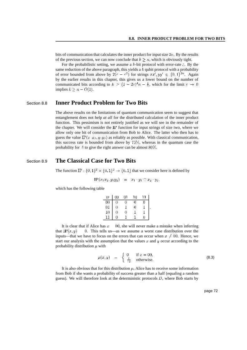
8.8. INNER PRODUCT PROBLEM FOR TWO BITS

bits of communication that calculates the inner product forinput size��. By the resultsof the previous section, we can now conclude that� �, which is obviously tight.

For the probabilistic setting, we assume a�-bit protocol with error-rate�. By thesame reduction of the above paragraph, this yields a� qubit protocol with a probabilityof error bounded from above by�� for strings�� . Againby the earlier results in this chapter, this gives us a lower bound on the number ofcommunicated bits according to� ��

� , which for the limit � � �implies� � ��.

Section 8.8 Inner Product Problem for Two Bits

The above results on the limitations of quantum communication seem to suggest thatentanglement does not helpat all for the distributed calculation of the inner productfunction. This pessimism is not entirely justified as we willsee in the remainder ofthe chapter. We will consider the

��function for input strings of size two, where we

allow only one bit of communication from Bob to Alice. The latter who then has toguess the value

�� as reliably as possible. With classical communication,this success rate is bounded from above by

��, whereas in the quantum case the

probability for� to give the right answer can be almost��

.

Section 8.9 The Classical Case for Two Bits

The function��

� �� that we consider here is defined by

�� which has the following table

IP��

��

.

It is clear that if Alice has� � ��, she will never make a mistake when inferring

that��

. This tells us—as we assume a worst case distribution over theinputs—that we have to focus on the errors that can occur when� ��

. Hence, westart our analysis with the assumption that the values� and� occur according to theprobability distribution� with

��

if � � ��,�� otherwise.

(8.3)

It is also obvious that for this distribution�, Alice has to receive some informationfrom Bob if she wants a probability of success greater than a half (equaling a randomguess). We will therefore look at the deterministic protocols

�, where Bob starts by

page 72

8.9. THE CLASSICAL CASE FOR TWO BITS

sending the bit value� � �

if his � is element of some set�� ,and otherwise the value

� � � if � � ��. (With �� and�� , see the introduction in Section 4.4.) After this, Alice hasto guessthe value of

�� on the basis of her string� and the received bit�. By simply

going through all the options for�� and�� (essentially�), in combination with the

rational choose for Alice (in the light of the assumed distribution�), we can see thatthe following four protocols each have the lowest possible error probability of

�out of

�� .��: The two� sets are�� and�� . Alice’s answer will

simply equal this bit�.

�: If �� and�� then�’s guess is calculated by NOT��.

��: The final answer is NOT�� in combination with Bob’s sets�� and

�� .��: When Bob uses the sets�� and�� , Alice answers

“�� ” if her � � ��and “

�� ” otherwise.

Moreover, if we look at the values� and � for which the above protocols make amistake (which happens only when

� � �), then we see that the error probability isequally distributed over the�� pairs

�� with ��

:

Protocol�� the

�combinations

�� that�� answers incorrectly

�� , �� and��

� �� , �� and��

�� , �� and��

�� , �� and��

.

This suggests a probabilistic protocol that uses two publiccoin flips to chooserandomly between

�� . The following procedure is indeed the best that Al-ice and Bob can do in the classical case after having receivedtheir inputs�� :1: Randomization Alice and Bob determine at random which one of the four deter-

ministic protocols�� or

�� they are going to use.

2: Bob’s communication Depending on his input� and the chosen protocol��, Bob

sends a “zero” or a “one” to Alice. (See the above list of protocol description forthe specifications).

3: Alice’s answer If Alice has� � ��she concludes “

�� ”; otherwise, she

acts in accordance with the protocol�� that was chosen at the first stage.

This communication protocol makes no mistake if� � ��and by its randomization

errs with �� in all the other cases. Therefore, a) there exists no input distribution�� that causes a higher error rate than�� , and b) the distribution� as defined in Equa-tion 8.3 reaches the�� bound and is hence an example of a worst case situation. Inother words,

�� is the highest possible correctness ratio in the classical setting. Thenext section shows that this can be improved if we allow Aliceand Bob to use priorentanglement.

page 73

8.10. THE QUANTUM IMPROVEMENT

Section 8.10 The Quantum Improvement

Here we will show that there is a one bit quantum protocol thatthat has a correctnessrate of

��, which improves the classical bound by almost four percent.The two parties have prior entanglement by the standard pair

�� . Depending on his input�, Bob first applies an operation�� to his��. Afterthis, a measurement is performed on the rotated qubit, yielding a classical bit

�that is

sent to the other party. If the receiver, Alice, has� � ��, she knows with certainty that

�� without having to interact with Bob. If this is not the case (� ��

), sheperforms a unitary transformation�� to her�� and measures the qubit in the standardbasis with outcome�. Alice’s ‘guess’ for

�� will now be the parity bit�� .

With the following rotations for� and�, this protocol will have a correctnessprobability of � � ��

� � �� for the worst case� �� . (If � � ��

, the correctnessrate is��.) Hence, the quantum protocol is more reliable than any classical proce-dure for this particular problem. The� and� rotations that establish this separationare (with

� � �� ):��

��

��

��

��

��

��

��

�

and

��

��

� ��

(In case the reader is wondering about the ratio behind this protocol, the entries of theabove matrices were obtained with the help of a computer program that performed anumerical search for the optimal solution of the inner product problem. The corre-sponding analytical expressions were inferred and verifiedby the author of the com-puter program.)

Section 8.11 Communication Complexity versus Quantum Mechan-ics

We have reached the stage where we are convinced that quantummechanicssometimesallows a significant reduction in communication complexity, but also sometimes doesnot. “The influence that quantum physics has on the theory of distributed computation

page 74

8.11. COMMUNICATION COMPLEXITY VERSUS QUANTUM MECHANICS

is significant but subtle”, should be the tantalizing conclusion for computer scientists.But, to paraphrase Dr Johnson[12], “If physics kicks computer science, should physicsnot be kicked back?” That is, what can we learn about nonlocality and quantum me-chanics from the theory of communication complexity?

The next chapter—which will be the last one before the Conclusion of this thesis—tries to initiate such a ‘back-action’. It will be shown thatthe limits of nonlocalitycoincide with the limits of distributed computing and that both of them can be viewedas a refinement of the ‘no-signaling theorem’.

page 75

Chapter 9

Superstrong Correlations versusCommunication Complexity

How close is the relation between nonlocality and communication with prior entangle-ment? What are the implications of the no-signaling theoremfor the nonlocal behaviorof physics and communication complexity? In this chapter, we will touch on these andrelated questions. We do this by imagining a toy-theory where theCHSH inequality forlocality is maximally violated (stronger than is possible in quantum mechanics) whilestill respecting the axiom of no-signaling. It will be shownthat in such a scenario,the communication complexity of a distributed decision problem becomes a vacuousconcept: it will always be one bit. This approach is inspiredby the work of Popescuand Rohrlich who, in a series of articles, asked the question: “Why is Nature not morenonlocal than she is?”

Section 9.1 Nonlocality Revisited

The Clauser, Horne, Shimony and Holt (CHSH ) inequality for classical theories givesa bound on the strength of correlations between two separated experiments.[22] Wedescribed this nonlocality argument earlier in this thesis, so we will here directly stateit in the form as we will use it in the rest of this chapter.

Imagine two separated parties� and�, each of which can perform one out of twoexperiments on a particle that they receive from a common source. There are there-fore four experimental set-ups that can apply to the combined system:

�� ,�� , �� and�� . The two possible outcomes of the measure-

ments on each side are labeled “�” and “�”, and we will call the�-particle system��.

We repeat the experiment many times such that we have an accurate estimation of allthe possible correlations between the different measurements and their outcomes. Asit is understood that for each trial we will always use the same state-preparation of��, we drop the conditional part when expressing the probabilities. For example, theprobability that both Alice and Bob measure a “one” when theyuse the measurementsettings�� and�� is denoted by

�� .

page 76

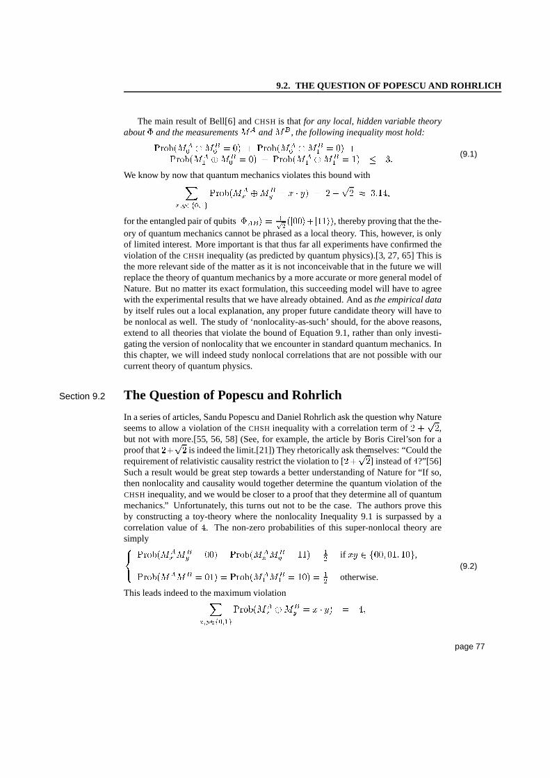
9.2. THE QUESTION OF POPESCU AND ROHRLICH

The main result of Bell[6] andCHSH is thatfor any local, hidden variable theoryabout� and the measurements� and�, the following inequality most hold:

�� (9.1)

We know by now that quantum mechanics violates this bound with

��

�� for the entangled pair of qubits

�� , thereby proving that the the-ory of quantum mechanics cannot be phrased as a local theory.This, however, is onlyof limited interest. More important is that thus far all experiments have confirmed theviolation of theCHSH inequality (as predicted by quantum physics).[3, 27, 65] This isthe more relevant side of the matter as it is not inconceivable that in the future we willreplace the theory of quantum mechanics by a more accurate ormore general model ofNature. But no matter its exact formulation, this succeeding model will have to agreewith the experimental results that we have already obtained. And asthe empirical databy itself rules out a local explanation, any proper future candidate theory will have tobe nonlocal as well. The study of ‘nonlocality-as-such’ should, for the above reasons,extend to all theories that violate the bound of Equation 9.1, rather than only investi-gating the version of nonlocality that we encounter in standard quantum mechanics. Inthis chapter, we will indeed study nonlocal correlations that are not possible with ourcurrent theory of quantum physics.

Section 9.2 The Question of Popescu and Rohrlich

In a series of articles, Sandu Popescu and Daniel Rohrlich ask the question why Natureseems to allow a violation of theCHSH inequality with a correlation term of� � ��,but not with more.[55, 56, 58] (See, for example, the articleby Boris Cirel’son for aproof that�� is indeed the limit.[21]) They rhetorically ask themselves: “Could therequirement of relativistic causality restrict the violation to [��] instead of�?”[56]Such a result would be great step towards a better understanding of Nature for “If so,then nonlocality and causality would together determine the quantum violation of theCHSH inequality, and we would be closer to a proof that they determine all of quantummechanics.” Unfortunately, this turns out not to be the case. The authors prove thisby constructing a toy-theory where the nonlocality Inequality 9.1 is surpassed by acorrelation value of�. The non-zero probabilities of this super-nonlocal theoryaresimply��

�� if �� ,�� otherwise.

(9.2)

This leads indeed to the maximum violation

��

��

page 77

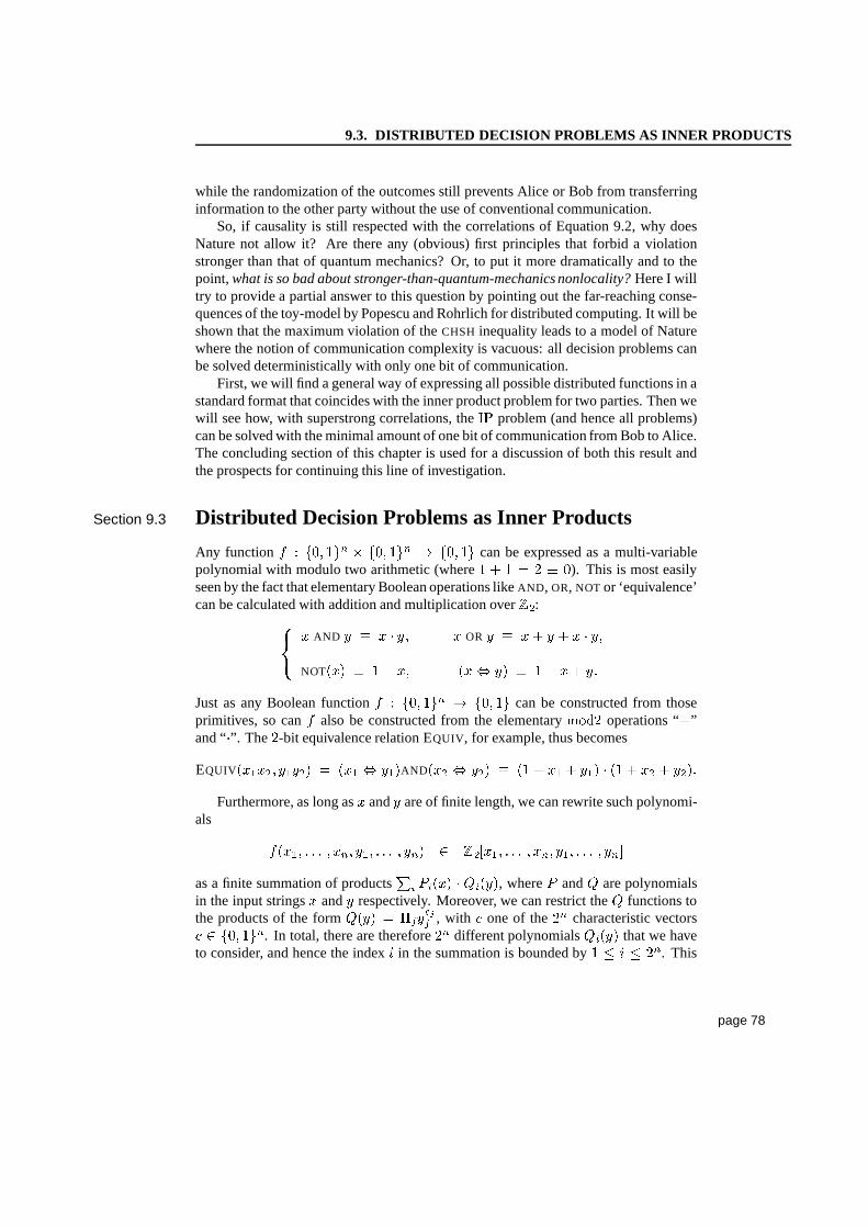
9.3. DISTRIBUTED DECISION PROBLEMS AS INNER PRODUCTS

while the randomization of the outcomes still prevents Alice or Bob from transferringinformation to the other party without the use of conventional communication.

So, if causality is still respected with the correlations ofEquation 9.2, why doesNature not allow it? Are there any (obvious) first principlesthat forbid a violationstronger than that of quantum mechanics? Or, to put it more dramatically and to thepoint,what is so bad about stronger-than-quantum-mechanics nonlocality?Here I willtry to provide a partial answer to this question by pointing out the far-reaching conse-quences of the toy-model by Popescu and Rohrlich for distributed computing. It will beshown that the maximum violation of theCHSH inequality leads to a model of Naturewhere the notion of communication complexity is vacuous: all decision problems canbe solved deterministically with only one bit of communication.

First, we will find a general way of expressing all possible distributed functions in astandard format that coincides with the inner product problem for two parties. Then wewill see how, with superstrong correlations, the

��problem (and hence all problems)

can be solved with the minimal amount of one bit of communication from Bob to Alice.The concluding section of this chapter is used for a discussion of both this result andthe prospects for continuing this line of investigation.

Section 9.3 Distributed Decision Problems as Inner Products

Any function�

� �� can be expressed as a multi-variablepolynomial with modulo two arithmetic (where��

). This is most easilyseen by the fact that elementary Boolean operations likeAND, OR, NOT or ‘equivalence’can be calculated with addition and multiplication over

�:��

� AND � � � � �� OR � � � � � � � � ��NOT

�� Just as any Boolean function

�� can be constructed from those

primitives, so can�

also be constructed from the elementary�� operations “�”and “�”. The �-bit equivalence relation EQUIV, for example, thus becomes

EQUIV�� AND

�� Furthermore, as long as� and� are of finite length, we can rewrite such polynomi-

als

� �� as a finite summation of products�� , where

�and� are polynomials

in the input strings� and� respectively. Moreover, we can restrict the� functions tothe products of the form�� , with � one of the�� characteristic vectors� � �� . In total, there are therefore�� different polynomials�� that we haveto consider, and hence the index

�in the summation is bounded by� � � � ��. This

page 78

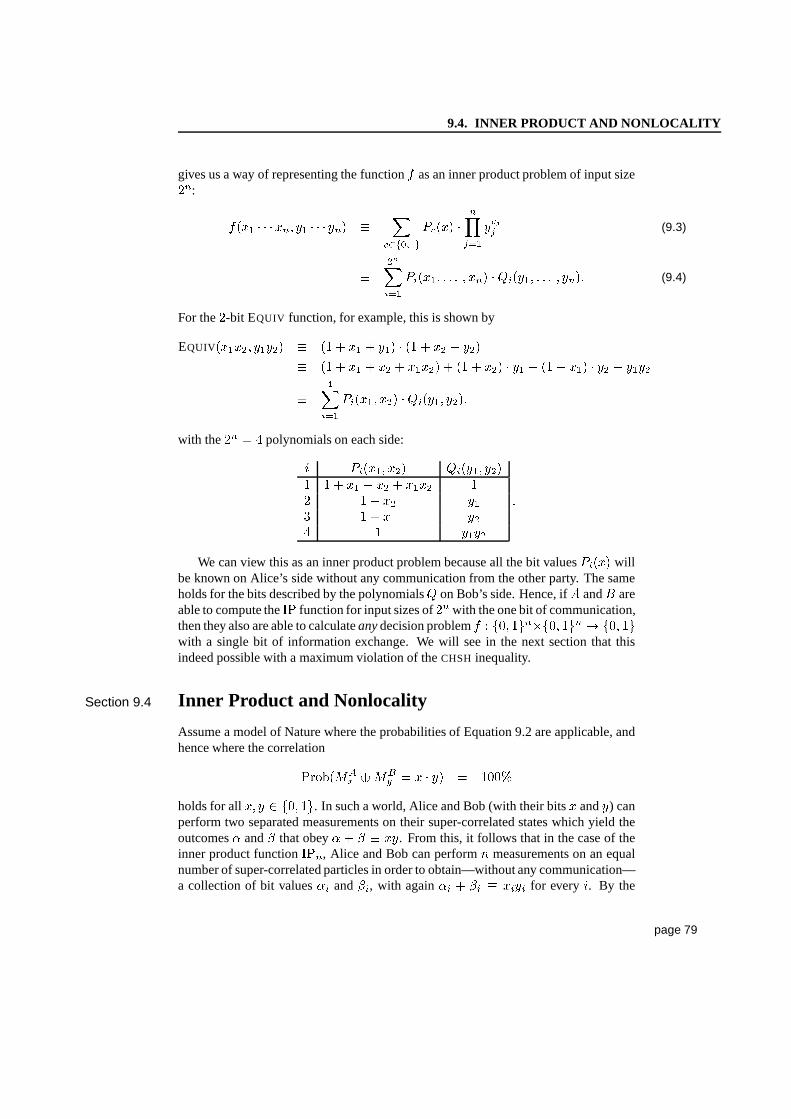
9.4. INNER PRODUCT AND NONLOCALITY

gives us a way of representing the function�

as an inner product problem of input size��:

� ��

��

�� (9.3)

��

�� (9.4)

For the�-bit EQUIV function, for example, this is shown by

EQUIV��

��

��

�

��

with the�� polynomials on each side:

� ��

�

We can view this as an inner product problem because all the bit values�� will

be known on Alice’s side without any communication from the other party. The sameholds for the bits described by the polynomials� on Bob’s side. Hence, if� and� areable to compute the

��function for input sizes of��with the one bit of communication,

then they also are able to calculateanydecision problem�

� �� with a single bit of information exchange. We will see in the next section that thisindeed possible with a maximum violation of theCHSH inequality.

Section 9.4 Inner Product and Nonlocality

Assume a model of Nature where the probabilities of Equation9.2 are applicable, andhence where the correlation

��

holds for all�� . In such a world, Alice and Bob (with their bits� and�) canperform two separated measurements on their super-correlated states which yield theoutcomes� and� that obey� � � � ��. From this, it follows that in the case of theinner product function

��, Alice and Bob can perform� measurements on an equal

number of super-correlated particles in order to obtain—without any communication—a collection of bit values�� and��, with again�� for every

�. By the

page 79

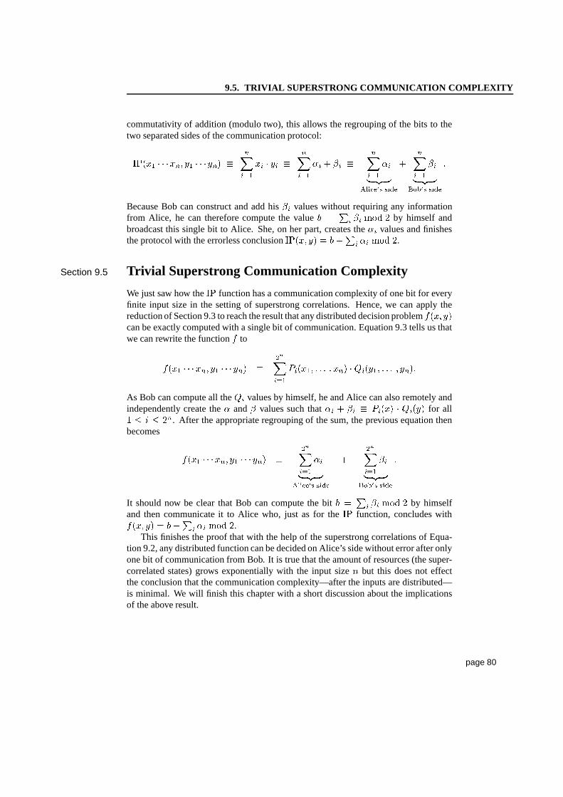
9.5. TRIVIAL SUPERSTRONG COMMUNICATION COMPLEXITY

commutativity of addition (modulo two), this allows the regrouping of the bits to thetwo separated sides of the communication protocol:

��

��

�

��

��

��

��

�

Because Bob can construct and add his�� values without requiring any informationfrom Alice, he can therefore compute the value

� � �� by himself andbroadcast this single bit to Alice. She, on her part, createsthe�� values and finishesthe protocol with the errorless conclusion

�� .

Section 9.5 Trivial Superstrong Communication Complexity

We just saw how the��

function has a communication complexity of one bit for everyfinite input size in the setting of superstrong correlations. Hence, we can apply thereduction of Section 9.3 to reach the result that any distributed decision problem

� ��can be exactly computed with a single bit of communication. Equation 9.3 tells us thatwe can rewrite the function

�to

� ��

�� As Bob can compute all the�� values by himself, he and Alice can also remotely andindependently create the� and� values such that�� for all� � � � ��. After the appropriate regrouping of the sum, the previous equation thenbecomes

� ��

��

� ��

��

It should now be clear that Bob can compute the bit� � �� by himself

and then communicate it to Alice who, just as for the��

function, concludes with� �� .This finishes the proof that with the help of the superstrong correlations of Equa-

tion 9.2, any distributed function can be decided on Alice’sside without error after onlyone bit of communication from Bob. It is true that the amount of resources (the super-correlated states) grows exponentially with the input size� but this does not effectthe conclusion that the communication complexity—after the inputs are distributed—is minimal. We will finish this chapter with a short discussion about the implicationsof the above result.

page 80

9.6. DISCUSSION

Section 9.6 Discussion

We can now rephrase our original question as, “What is so bad for Nature about super-efficient distributed computing?” It is not clear if there isa convincing answer to thisquestion, as it does not seem to conflict with any physical intuition. But trivial com-munication complexitydoesdisprove the existence of an intrinsic ‘complexity’ fordistributed tasks. Even if we need an exponential amount of prior superstrong en-tanglement (as is indeed the case in the derivation of Section 9.5), the solution of allpossible distributed functions with a single bit of communication surely does contra-dict our experiences in computer science. Much as in computability theory, there isa hierarchy of different ‘classes’ of communication problems.[4] Such hierarchies areat the core of theoretical computer science, and their ‘collapse’—as happened here byassuming superstrong correlations—goes against the intuition of most researchers inthe field of complexity theory.

Future investigations along the lines of this chapter can beaimed at obtaining otherimplications of stronger-than-quantum-mechanics correlations. What happens, for ex-ample, if we assume a violation of theCHSH inequality with a factor less than thefour we used here, say with

� �? This is still stronger than allowed by the the nonlo-cality of quantum mechanics, but the consequences for communication complexity areless clear in this scenario. Also, the possible implications for computationalclassesdeserve further research. One can thus investigate how the existence of superstrongcorrelations would enhance the power of, say, logarithmic depth circuits. Could it bethe case that this class NC��

�contains all of P? And even beyond that, what can be

computed in polynomial time under the assumptions of this chapter? The conjecturethat superstrong nonlocality would imply NP�P��

�, is certainly a tempting thought.

page 81

Chapter 10

Conclusion

In this last, chapter I will describe some of the work on communication complexitydone by other authors. This review is concluded with an outline for future research.Finally, the possibilities of experiments that implement one of the protocols will be dis-cussed. We derive some threshold values for the realistic setting of noisy entanglementand faulty detectors. These criteria for a proper quantum communication protocol referdirectly to some of the loopholes that exist for the experimental verification of Nature’snonlocality.

Section 10.1 Other Work on Quantum Communication

Soon after the first publication of a separation between quantum and classical commu-nication complexity[23], other, more spectacular, results were obtained. Besides theones described in this thesis, the following results shouldbe mentioned.

In 1997, Harry Buhrman, Richard Cleve and Avi Wigderson obtained an almostquadratic separation for the well-known two-party disjointness problem in the random-ized setting.[17] In the same article, they also showed an exponential difference be-tween quantum and classical communication for a deterministic, promise problem thatis based the on Deutsch-Jozsa algorithm.[26] The function for the quadratic separationtells if two sets� �� are disjoint or not. Hence,

DISJOINT��

��NOT

�� where� and � � �� are the characteristic vectors for the sets� and

�. The

authors recognized that this function is a distributed caseof a database search for anindex

�such that

�� . Hence, by applying Lov Grover’s search algorithm[14,31, 32] while sending the index register of size��back and forth

�� times, Aliceand Bob can solve this problem with

�� bits of communication. As it wasalready known that a probabilistic solution of the DISJOINT function requires��bits of communication[38] in the classical setting, this established a near quadraticseparation.

page 82

10.2. OPEN PROBLEMS AND FUTURE RESEARCH

The exponential difference is possible for the deterministic, promise problem wherethe function DDJ (‘distributed Deutsch-Jozsa’) is defined by

�� if the string� � � is ‘balanced’,

� if the string� � � is ‘constant’,

where� � � is the bitwiseEXCLUSIVE OR of the � bits�� ,

and the promise on� and� is that this string is either balanced or constant. For thequantum solution of this problem, Bob starts by preparing the state of�� qubits�� , which is then teleported to the other party (requiring� �� bits ofcommunication). Alice, on her side, changes this received state to the final superposi-tion �� , which enables her to decide without error if�� is balancedor not. The proof that of the order of� bits of communication are necessary withoutquantum resources is rather involved and can be found in the original article. The expo-nential separation by Andris Ambainis, Leonard Schulman, Amnon Ta-Shma, UmeshVazirani and Avi Wigderson improves the previous result in that it holds for the morerealistic probabilistic setting.[1] It should be mentioned, however, that the distributed‘sampling’ problem of this article lies outside the standard communication model: it isa not a decision problem, but a multi-valued function instead.

The strongest separation that we currently have was established by Ran Raz in1999.[57] The problem that is analyzed in this article is defined follows. Alice receivesa unit vector�� and two mutually orthogonal subspaces�, � � �� . The inputof Bob consists of a rotation

� � ��. The question that Alice has to answer nowis: “Is

� �� an element (within some error margin) of� or of �?” The input forboth parties consists of� real variables. In the approximating variant, each variableis described by�� bits, which leads to a total input size of�� . Therestriction on the inputs is the promise that

� �� will lie in either� or �, but not inboth. Using teleportation, it is reasonably straightforward to design a quantum protocolwith complexity

�� for this problem. The significance of Raz’s work lies in the�� lower bound he obtains for the probabilistic, classical procedures.

Section 10.2 Open Problems and Future Research

An important open problem in the theory of quantum communication is the poten-tial difference between the qubit and the entanglement model of communication (cf.Section 4.10). We know that every qubit of communication canbe simulated with anentangled pair and two classical bits of communication, butwhat about the inverse ofthis simulation? Is it always the case that� bits of communication in combination witha potentially unbounded amount of entanglement can be converted into a protocol thatuses

�� qubits of communication but no prior entanglement? If thereexists such aconversion, then the qubit model and the entanglement modelare effectively the same.But if this is not the case, then we have to conclude that the quantum complexity of adistributed function consists of two distinct components:1) the amount of prior entan-glement, and 2) the number of communicated bits, where the first can be much largerthan the second.

page 83

10.3. THRESHOLDS FOR EXPERIMENTAL IMPLEMENTATIONS

We already mentioned the almost quadratic reduction in complexity for the DIS-JOINT function. This result is especially interesting as this function plays a role incommunication complexity comparable to the SATISFIABILITY problem for computa-tional tasks. In [4], it was shown by Babaiet al. that it is a complete problem for thecommunication class co-NP��. Hence, the natural and open question of whether thereexists an

�� quantum protocol for the DISJOINT problem is equivalent to asking“NP�� BQP��?”, where we already know that NP�� BPP��.

This brings us to the most prominent open problem in in the field: Does there existan exponential separation between probabilistic classical and quantum communicationfor a function without a promise?We know by the work of Bealset al. that in theblack-box model of computation there can only be a polynomial difference betweenclassical and quantum computers.[5] One wonders if this also holds for communicationproblems, and if so, if the ‘lower bounds by polynomials’ methods of this publicationalso translates to our setting. Recently, Harry Buhrman andRonald de Wolf have madea significant first step in this direction[18]. Yet it is stillunknown how far nonlocalitywill take us from traditional communication.

Section 10.3 Thresholds for Experimental Implementations

Our last discussion in this thesis will be about the experimental feasibility of simplequantum communication protocols. Various experimental results have already con-firmed the nonlocal predictions of quantum mechanics.[3, 27, 65] More recent ideaslike superdense coding or teleportation have also found their way into the laboratory.(See [11, 13, 28, 44] for some examples.) It is therefore natural to wonder if it is pos-sible with current technology to implement the protocols ofthis thesis, and what thecriteria are for a ‘successful experiment’.

In communication complexity theory, we compare procedureson the basis of theamount of information that the parties have to exchange to solve a distributed task. Thishas the fortunate consequence that we are not concerned withthe possibility of ‘somekind of hidden signaling between� and�’, and hence with the criterion of space-like-separation for the measurements� and�. It is perfectly in order for Alice andBob, to have received the prior entanglement and the data a long time before the actualexecution of the protocol. The only resource that counts in the context of this thesisis the number of (quantum) bits that the parties have to communicate. Hence, we cansafely disregard the potential ‘hidden’ communication between the entangled quantumstates. Not because it cannot occur, but because it does not count.

The detector efficiency, on the other hand,doesplay an important role. It increasesthe complexity of the quantum protocol if Alice sometimes has to inform Bob that herphoton detection failed and that the experiment has to be repeated. Assume, for exam-ple, that the error-rate of the detector is so high, that there exists a classical model forthe experiment that gives the same predictions (see [52] foran explanation of this pos-sibility). Then, by the same token, there also exists a classical procedure that achievesthe same correctness ratio as the quantum protocol. Hence, the existence of such a‘detector loophole’ indicates that the quantum mechanicalexperiment does not give animprovement of over the classical lower bound. In the next sections, we derive some

page 84

10.4. THRESHOLDS FOR A ONE BIT PROTOCOL

thresholds for the error-rate of the detectors and the noiseof the entangled states, thattruly separate quantum communication from its classical pendant.

Section 10.4 Thresholds for a One Bit Protocol

Consider the two-party protocol that uses one bit of communication and an entangledpair

�� . (See, for example, the protocols of Chapter 5 or Sec-tion 8.8.) Let

�� be the success rate of the quantum procedure under perfect conditions,

which is higher than the classical bound��. We will answer two questions for this set-

ting: “What is the amount of noise that we can allow for�?” and “What efficiency isrequired for the detection or measurement of the qubits?”

Section 10.5 Noisy Entangled States

Let�� be the probability that Alice and Bob have a random� qubit state rather

than the desired entangled pair�. The density matrix�� of this mixture reads in thecomputational basis as

��

��

��

��

� � � ��

��

The expected probability of success,� ��

, for the quantum procedure with this noisystate is�

�� (under the worst-case assumption that the quantum protocolwith

the completely noisy state corresponds to a coin flip, and hence has an error rate of��

). By the equation� ��

�, this gives the threshold on the quality of the state��

of

� ��

��

� �As an aside, it is interesting to combine the�-threshold with the observation in Sec-

tion 2.2 that for�� the state�� is disentangled. If this is the case, then the quantum

protocol can always be simulated by a classical procedure using the decomposition intensor-products of the state��. Hence we have also a bound on how much

�� and

��

can differ:��

��

� �� .

Chapter 5 gave the example of a function for which�� and

�� .

These values give us the criterion� � �� for the purity of the state�. This

is definitely feasible for entangled photons, for which� rates close to��

are alreadypossible.

Section 10.6 Inexact Measurement Devices

An apparatus that tries to implement a measurement can have two kinds of errors: itgives a random answer, or it gives no answer at all. (The advantage of the second

page 85

10.7. CONCLUSION

is that the party then at least knows that something went wrong.) The probability ofan incorrect answer can be rephrased as a perfect measurement on a noisy state, thecase which we analyzed in the previous section. A faulty measurement that producesa random outcome with probability

�� is equivalent to a perfect measurement onthe noisy state��. If we combine such an imperfect measurement device with a noisystates��, we get a total eta factor of� � � � .

Now we will focus on the second scenario, where there is a probability��

� thata party is not able to read out the (otherwise perfect) measurement outcome. This givesthe probability�

that the protocol is executed without any problems,��

� thatone of the parties does not measure an outcome, and the remaining

�� thatboth

parties do not obtain a measurement result. When a detectionerror occurs, Alice andBob can adopt the strategy that they try to execute the best possible classical procedureas an alternative. This back-up plan will have a correctnessprobability of

��

in thecase that both sides have such an error (the probability

�� ). If only one party has

a problem with his or her measurement, then the protocol willcorrespond again to ablind guess. The overall success of this approach is thus calculated by� �

��

��

��

��

leading to the lower bound for the ‘visibility’ of the qubits

� ��

��

� � ��

For the earlier�� and

��

� , this gives the threshold of� bigger than�� . For photon detections, the detector efficiency threshold is by far themost problematic as state-of-the-art experiments are still limited by a� of the order of�� to ��.

Section 10.7 Conclusion

In this thesis we saw how one can translate the nonlocal phenomena of quantum physicsinto communication protocols that are more efficient than classical procedures. Theseresults highlight the differences between classical and quantum information in waysimilar to that of quantum computation.

The implementation of a quantum protocol that is truly more efficient than anyclassical procedure is problematic because of the detectorinefficiency of our currentmeasurement devices. But, as for the detector loophole for nonlocality experiments, itis not inconceivable that in the near future a sufficiently reliable measurement devicecan be employed to overcome this barrier.

It is debatable if quantum communication will ever reach thestatus of a ‘commer-cial application’. But even if it does not, its ideas will still remain a powerful tool tounderline, explain and investigate the differences between a universe that is governedby classical laws and the one that we are living in.

page 86

Appendix A

Appendix to Holevo’s Bound

‘Holevo’s bound’puts a limit on the amount of classical information that can be trans-mitted with quantum signals. One consequence of this celebrated result is the observa-tion that a�-dimensional closed quantum system can carry no more information than aclassical system of the same dimension:�� bits. More precisely, Holevo’s theoremestablishes an upper bound on the mutual information� �� between the sourceBob and the receiver Alice according to� �� . (See [25, 61] for the notionof ‘mutual information’.) This bound

�� is calculated as follows.By � � �� , we indicate a source that transmits its codewords�� with

probability��. The ‘average’ codeword for such a� is thus expressed by� ��.With this �, thechi quantity of a source is defined by

�� where

�denotes the Von Neumann entropy of a quantum mechanical mixture.

Before we extend this result, we will first take a closer look at the above theoremand try to understandwhythe information transfer is bounded by the difference betweenthe two terms

�� and�� .Section A.1 Information Transfer with Quantum States

Bob can send information if he is able to change the state of Alice in such a waythat she on her side can detect this change. The bigger the state space of the changeis, the more information can be transfered by it. This is captured by the positiveterm “

�� ” in Holevo’s bound, which expresses the randomness�� that Bob can cause on Alice’s side. Here we already see that the informationtransfer is fundamentally bounded by the dimension of the system (because

�� Dim��), independently of the number of messages�� that Bob uses. This phe-

nomenon is most clearly at work when we allow the whole continuum of one-qubitstates�� . Such a source gives an uncountable infinite set ofpossible signals that Alice can receive, yet she will not be able to infer more than

page 87

A.2. HOLEVO’S BOUND VERSUS SUPERDENSE CODING

one bit of information per received signal from it. This is due to the small distin-guishability between most of the messages: on paper it may seem that

�� and�� are very different, but the physical reality is that theyare very similar. In every possible situation (allowed by quantum mechanics),� willbehave almost the same as

�. It is therefore very hard for Alice to discover which one

of the states she has received. All this is captured by the small entropy of the equalmixture

�� .The second, negative, term in Holevo’s bound tells us that the randomness

�� hasto be related to the probabilities�� for the different messages, and not the individualentropies

��. It is not sufficient for Bob to cause a big random effect on theotherparty’s side. For if he wants to convey a message

�, there also has to be a strong,

detectable correlation between the�

and its carrier��. Such a correlation is indicatedif the randomness of� disappears when we know the index

�that Bob has used. But if

the signals�� by themselvesare very random,i.e. their entropies�� are high, then

this will decreasethe effectiveness of the source� � �� . This justifies thesubtraction of the sum�� .

Section A.2 Holevo’s Bound versus Superdense Coding

Is superdense coding not a violation of Holevo’s bound? Are we not using one qubit totransmit two bits of information? No, we are not. It is true that Bob only sends a singlequbit to Alice but this signal is part of a bigger four-dimensional (�-qubit) system thatcancarry the two bits of information. This is again an example where we have to payattention to the fact that entangled qubits should be viewedas a single system.

But is it then also possible to come up with a protocol where the parties initiallyshare� entangled pairs, where after the transmission of one qubit more than two bits ofinformation has been communicated? The following extension of Holevo’s bound byMichael Nielsen tells us that this is not possible and that superdense coding is indeedthe best we can do.

Section A.3 Holevo’s Bound in the Presence of Entanglement

How much can the mutual information� �� of Alice increase if she receives onequbit from Bob? Let� � �� (with the average state� � �� ) be thesituation before the communication of the qubit�, and�� (with �� ) the situation afterwards. This�� is the joint system of� and �, hence wecan use both the subadditivity rule and the Araki-Lieb inequality[2], which tell us that�� for quantum systems

�and�. In our case�

is Alice’s initial state�� and� is the single qubit�� (with� � �� ), implying

the bound�� (A.1)

� �� (A.2)

page 88

A.3. HOLEVO’S BOUND IN THE PRESENCE OF ENTANGLEMENT

where the square brackets indicate the application of the subadditivity/Araki-Lieb re-sult.

Besides the above scenario, other activities during a quantum communication pro-tocol are: 1) unitary operations on Alice or Bob’s side and 2)the communication ofquantum information from Alice to Bob. The entropy

�of a quantum system is in-

variant under unitary transformations, and it also known that tracing out a qubit (whichis what effectively happens on Alice’s side when she sends a qubit to Bob) cannot in-crease the value of

�

. We have thus reached the conclusion that the mutual informationon Alice’s side,� �� , can only increase if she receives a qubit from the otherparty, and that this increase per qubit is bounded from aboveby � bits. This bound isobtained if� and� share initial entanglement and use the superdense coding protocolfrom Bob to Alice to send information.

Furthermore we can also analyze the scenario where the parties do not share initialentanglement. This can be rephrased as the situation where Alice starts with a fixedpure state�� and hence with

�� . This term

��bounds the mutual informationfrom above by� �� and can only increase with one bit when Aliceor Bob sends a qubit to the other party. Therefore, in this setting the total amountof communication has to be at least� bits if Alice wants to obtain� bits of mutualinformation from Bob. This result will be clarified for two standard protocols.

Classical communication from Bob to Alice: Alice starts with a zero register�� andevery time Bob sends her a classical bit of information, the chi factor increaseswith one bit as

�� and�� remains zero. After� bits ofcommunication, this establishes� �� .

Superdense coding from Bob to Alice:First, Alice distributes� entangled pairs be-tween her and Bob (we assume that� is even). This requires� qubits of com-munication from� to � and yields the intermediate situation on her side with�� and hence

� � �. After that, Bob uses the entangled

pairs for superdense coding, thereby reaching the bound of Equation A.2 andcommunicating� bits to Alice.

The main implication of this is that even if Alice is allowed to send out an unlimitedamount of qubits (to create entanglement between her and other parties, for example),it will still be necessary for� to send�� qubits back to� to convey� bits of in-formation to her. This immediately puts a limit on the usefulness of entanglement forinformation transmission: the factor� reduction of superdense coding is the highestpossible.

This result is an expansion of Holevo’s bound, as it encapsulates a more generalsetting where two-way communication is allowed between� and� instead of the oneway communication of the earlier theorem.

page 89

Bibliography

[1] Andris Ambainis, Leonard J. Schulman, Amnon Ta-Shma, Umesh Vazirani, andAvi Wigderson. The quantum communication complexity of sampling. In Pro-ceedings of the 39th Annual Symposium on Foundations of Computer Science(FOCS’98), pages 342–351, Los Alamitos, California, November 1998. IEEEComputer Society Press.

[2] Huzihiro Araki and Elliott H. Lieb. Entropy inequalities. Communications inMathematical Physics, 18:160–170, 1970.

[3] Alain Aspect, Jean Dalibard, and Gerard Roger. Experimental test of Bell’s in-equalities using time-varying analyzers.Physical Review Letters, 49:1804–1807,1982.

[4] Laszlo Babai, Phyllis G. Frankl, and Janos Simon. Complexity classes in com-munication complexity theory. InProceedings of the 27th IEEE Symposium onFoundations of Computer Science, pages 337–347, Los Angeles, Ca., USA, Oc-tober 1986. IEEE Computer Society Press.

[5] Robert Beals, Harry Buhrman, Richard Cleve, Michele Mosca, and Ronaldde Wolf. Quantum lower bounds by polynomials. InProceedings of the 39thAnnual Symposium on Foundations of Computer Science (FOCS’98), pages 352–361, Los Alamitos, California, November 1998. IEEE Computer Society Press.On the quant-ph archive, report no. 9802049.

[6] John S. Bell. On the Einstein-Podolsky-Rosen paradox.Physics, 1:195–200,1964.

[7] John S. Bell. Speakable and unspeakable in quantum mechanics. CambridgeUniversity Press, 1987.

[8] Charles Bennett and Stephen Wiesner. Communication viaone- and two-particleoperators on Einstein-Podolsky-Rosen states.Physical Review Letters, 69:2881–2884, 1992.

[9] Charles H. Bennett, Gilles Brassard, Claude Crepeau, Richard Josza, Asher Peres,and William K. Wootters. Teleporting an unknown quantum state via dual clas-sical and Einstein-Podolsky-Rosen channels.Physical Review Letters, 70:1895–1899, 1993.

page 90

BIBLIOGRAPHY

[10] Charles H. Bennett, Gilles Brassard, Sandu Popescu, Benjamin Schumacher,John A. Smolin, and William K. Wootters. Purification of noisy entanglementand faithful teleportation via noisy channels.Physical Review Letters, 76:722–725, 1996. On the quant-ph archive, report no 9511027.

[11] Danilo Boschi, Salvatore Branca, Francesco De Martini, Lucien Hardy, andSandu Popescu. Experimental realization of teleporting anunknown pure quan-tum state via dual classical and Einstein-Podolski-Rosen channels.Physical Re-view Letters, 80:1121–1125, 1998.

[12] James Boswell.The Life of Samuel Johnson. Penguin Classics. Penguin, London,1979. Edited by Christopher Hibbert.

[13] Dik Bouwmeester, Jian-Wei Pan, Klaus Mattle, Manfred Eibl, Harald Weinfurter,and Anton Zeilinger. Experimental quantum teleportation.Nature, 390:575,1997.

[14] Michel Boyer, Gilles Brassard, Peter Høyer, and Alain Tapp. Tight bounds onquantum searching.Fortschritte der Physik, 46(4–5):493–505, 1998. On thequant-ph archive, report no. 9605034.

[15] Samuel L. Braunstein and Carlton M. Caves. Writing out better Bell inequalities.In Shun ichi Kobayashiet al., editor,Proceedings of the 3rd International Sympo-sium on the Foundations of Quantum Mechanics in the Light of New Technology,pages 161–170. Physical Society of Japan, 1990.

[16] Harry Buhrman, Richard Cleve, and Wim van Dam. Quantum entanglement andcommunication complexity. Technical Report in the BRICS Research Series RS-97-40, BRICS, University of Aarhus (Denmark), January 1998. On the quant-pharchive, report no. 9705033.

[17] Harry Buhrman, Richard Cleve, and Avi Wigderson. Quantum vs. classical com-munication and computation. InProceedings of the 30th Annual ACM Sympo-sium on Theory of Computing (STOC’98), pages 63–68. ACM Press, 1998. Onthe quant-ph archive, report no. 9705033.

[18] Harry Buhrman and Ronald de Wolf. Communication complexity lower boundsby polynomials. cs.CC report 9910010, Los Alamos archive, October 1999.

[19] Harry Buhrman, Wim van Dam, Peter Høyer, and Alain Tapp.Multiparty quan-tum communication complexity.Physical Review A, 60(4):2737–2741, October1999. On the quant-ph archive, report no. 9710054.

[20] Benny Chor and Oded Goldreich. Unbiased bits from sources of weak random-ness and probabilistic communication complexity.SIAM Journal on Computing,17(2):230–261, April 1988.

[21] Boris S. Cirel’son. Quantum generalizations of Bell’sinequality.Letter in Math-ematical Physics, 4:93–100, 1980.

page 91

BIBLIOGRAPHY

[22] John F. Clauser, Michael A. Horne, Abner Shimony, and Richard A. Holt. Pro-posed experiment to test local hidden-variable theories.Physical Review Letters,23:880–884, 1969.

[23] Richard Cleve and Harry Buhrman. Substituting quantumentanglement for com-munication.Physics Review A, 56(2):1201–1204, August 1997. On the quant-pharchive, report no. 9704026.

[24] Richard Cleve, Wim van Dam, Michael Nielsen, and Alain Tapp. Quantum en-tanglement and the communication complexity of the inner product function. InColin P. Williams, editor,Proceedings of the 1st NASA International Confer-ence on Quantum Computing and Quantum Communications (QCQC’98), num-ber 1509 in Lecture Notes in Computer Science, pages 61–74. Springer-Verlag,1999. On the quant-ph archive, report no. 9708019.

[25] Thomas M. Cover and Joy A. Thomas.Elements of Information Theory. WileySeries in Telecommunications. John Wiley & Sons, Inc., 1991.

[26] David Deutsch and Richard Jozsa. Rapid solution of problems by quantum com-putation.Proceedings of the Royal Society of London A, 439:553–558, 1992.

[27] Stuart J. Freedman and John F. Clauser. Experimental test of local hidden-variabletheories.Physical Review Letters, 28:938–941, 1972.

[28] Akira Furusawa, Jens Lykke Sørensen, Samuel L. Braunstein, Christopher A.Fuchs, H. Jeff Kimble, and Eugene S. Polzik. Unconditional quantum teleporta-tion. Science, 282(5389):706–709, 1998.

[29] Michael R. Garey and David S. Johnson.Computers and Intractability (A guide tothe theory of NP-completeness). W.H. Freeman and Company, New York, 1979.

[30] Daniel M. Greenberger, Michael Horne, and Anton Zeilinger. Going beyondBell’s theorem. In Menas Kafatos, editor,Bell’s Theorem, Quantum Theory, andConceptions of the Universe, pages 69–72. Kluwer Academic, 1989.

[31] Lov K. Grover. A fast quantum mechanical algorithm for database search. InProceedings of the 28th Annual ACM Symposium on the Theory ofComputing(STOC’96), pages 212–219, Philadelphia, Pennsylvania, May 1996. ACM. Onthe quant-ph archive, report no. 9605043.

[32] Lov K. Grover. Quantum mechanics helps in searching fora needle in a haystack.Physical Review Letters, 79(2):325–328, july 1997. On the quant-ph archive,report no. 9706033.

[33] Lucien Hardy. A new way to obtain Bell inequalities.Physics Letters A, 161:21–25, 1991.

[34] Lucien Hardy and Wim van Dam. Quantum communication using a nonlocalZeno effect.Physical Review A, 59(4):2635–2640, April 1999. On the quant-pharchive, report no. 9805037.

page 92

BIBLIOGRAPHY

[35] Alexander S. Holevo. Bounds for the quantity of information transmitted by aquantum communication channel.Problemy Peredachi Informatsii, 9(3):3–11,1973. English Translation inProblems in Information Transmission, 9:177–183,1973.

[36] Michał Horodecki, Paweł Horodecki, and Ryszard Horodecki. Separability ofmixed states: Necessary and sufficient conditions.Physics Letters A, 223(1–2):1–8, November 1996. On the quant-ph archive, report no. 9605038.

[37] Michał Horodecki, Paweł Horodecki, and Ryszard Horodecki. Mixed-state en-tanglement and distillation: Is there “bound” entanglement in nature? PhysicalReview Letters, 80(24):5239–5242, June 1998. On the quant-ph archive, reportno. 9801069.

[38] Bala Kalyanasundaram and Georg Schnitger. The probabilistic communicationcomplexity of set intersection.SIAM Journal on Discrete Mathematics, 5(4):545–557, November 1992.

[39] Martin Kneser. Abschatzung der asymptotische Dichtevon Summenmengen.Mathematische Zeitschrift, 58:459–484, 1953.

[40] Donald E. Knuth. The Art of Computer Programming: Seminumerical Algo-rithms, volume 2. Addison-Wesley, Reading, Massachusetts, thirdedition, 1998.

[41] Ilan Kremer. Quantum communication. Master’s thesis,Computer Science De-partment, The Hebrew University of Jerusalem, March 1995.

[42] Eyal Kushilevitz and Noam Nisan.Communication Complexity. Cambride Uni-versity Press, Cambridge, United Kingdom, 1997.

[43] Henry B. Mann.Addition theorems: The addition theorems of group theory andnumber theory, volume 18 ofInterscience tracts in pure and applied mathematics.Interscience Publishers, New York, 1965. See page 6 for a proof of Kneser’sTheorem.

[44] Klaus Mattle, Harald Weinfurter, Paul G. Kwiat, and Anton Zeilinger. Dense cod-ing in experimental quantum communication.Physical Review Letters, 76:4656–4659, 1996.

[45] N. David Mermin. Boojums All the Way Through: Communicating Science in aProsaic Age. Cambridge University Press, Cambridge (England), 1990.

[46] N. David Mermin. What’s wrong with these elements of reality? Physics Today,43(6):9–11, June 1990.

[47] Roger B. Myerson.Game Theory: Analysis of Conflict. Harvard University Press,Cambridge, Massachusetts, 1991.

page 93

BIBLIOGRAPHY

[48] Ashwin Nayak. Optimal lower bounds for quantum automata and random accesscodes. InProceedings of the 40th Annual Symposium on Foundations of Com-puter Science (FOCS’99), pages 369–377, New York, NY, October 1999. IEEEComputer Society Press.

[49] John von Neumann. Zur theorie der gesellschaftsspiele. Mathematische Annalen,100:295–320, 1928. Translated in English in [50].

[50] John von Neumann. On the theory of games and strategy. InHarold W. Kuhnand Albert W. Tucker, editors,Contributions to the Theory of Games, Volume IV,volume 40 ofAnnals of Mathematics Studies, pages 13–42. Princeton UniversityPress, Princeton, New Jersey, 1959. English translation of[49].

[51] John von Neumann and Oskar Morgenstern.Theory of games and economicbehavior. Princeton University Press, Princeton, third edition, 1953.

[52] Philip M. Pearle. Hidden-variable example based upon data rejection.PhysicalReview D, 2(8):1418–1425, 1970.

[53] Asher Peres.Quantum Theory: Concepts and Methods, volume 72 ofFundamen-tal Theories of Physics. Kluwer Academic Publishers, Dordrecht, The Nether-lands, 1995.

[54] Asher Peres. Separability criterion for density matrices.Physical Review Letters,77:1413–1415, 1996. On the quant-ph archive, report no. 9604005.

[55] Sandu Popescu and Daniel Rohrlich. Quantum nonlocality as an axiom.Founda-tions of Physics, 24(3):379–385, 1994.

[56] Sandu Popescu and Daniel Rohrlich. The relativistic EPR argument. In Robert S.Cohen, Michael Horne, and John J. Stachel, editors,Potentiality, entanglementand passion-at-a-distance: quantum mechanical studies for Abner Shimony, Vol-ume Two, volume 194 ofBoston studies in the philosophy of science. Kluwer Aca-demic Publishers, Dordrecht, The Netherlands, 1997. On thequant-ph archive as“Action and Passion at a Distance: An Essay in Honor of Professer Abner Shi-mony”, report no. 9605004.

[57] Ran Raz. Exponential separation of quantum and classical communication com-plexity. In Proceedings of the 31st Annual ACM Symposium on Theory of Com-puting (STOC’99), pages 358–367, Atlanta, Georgia, May 1999. ACM Press.

[58] Daniel Rohrlich and Sandu Popescu. Nonlocality as an axiom for quantum theory.In Ady Mann and Micha Revzen, editors,The dilemma of Einstein, Podolskyand Rosen, 60 years later: International symposium in honour of Nathan Rosen,volume 12 ofAnnals of the Israel Physical Society, chapter 16. Israel PhysicalSociety, Haifa, Israel, 1996. On the quant-ph archive, report no. 9508009.

[59] Benjamin Schumacher. Sending quantum entanglement through noisy channels.Physical Review A, 54(4):2614–2628, October 1996. On the quant-ph archive,report no. 9604023.

page 94

BIBLIOGRAPHY

[60] Adi Shamir. Factoring numbers in�� arithmetic steps.Information Pro-

cessing Letters, 8(1):28–31, January 1979.

[61] Claude E. Shannon and Warren Weaver.The mathematical theory of communica-tion. University of Illinois Press, 1949.

[62] Euan J. Squires, Lucien Hardy, and Harvey R. Brown. Nonlocality from an ana-logue of the quantum Zeno effect.Studies in History and Philosophy of Science,25:425–435, 1994.

[63] Alan Turing. On computable numbers, with an application to the entschei-dungsproblem. Proceedings of the London Mathematical Society, Series 2,42:230–265, 1937.

[64] Umesh V. Vazirani. Towards a strong communication complexity theory or gener-ating quasi-random sequences from two communicating slightly-random sources.In Proceedings of the Seventeenth Annual ACM Symposium on Theory of Comput-ing, pages 366–378, Providence, Rhode Island, May 1985. ACM Press. Extendedabstract.

[65] Gregor Weihs, Thomas Jennewein, Christoph Simon, Harald Weinfurter, and An-ton Zeilinger. Violation of Bell’s inequality under strictEinstein locality condi-tions. Physical Review Letters, 81:5039–5043, 1998. On the quanth-ph archive,report no. 9810080.

[66] Reinhard F. Werner. Quantum states with Einstein-Podolsky-Rosen correlationsadmitting a hidden-variable model.Physical Review A, 40(8):4277–4281, 1989.

[67] William K. Wootters and Wojceich H. Zurek. A single quantum cannot be cloned.Nature, 299:802–803, October 1982.

[68] Andrew Chi-Chih Yao. Some complexity questions related to distributive com-puting. InProceedings of the 11th Annual ACM Symposium on Theory of Com-puting (STOC’79), pages 209–213, New York, 1979. ACM Press.

[69] Andrew Chi-Chih Yao. Quantum circuit complexity. InProceedings of the34th IEEE Symposium on Foundations of Computer Science, pages 352–361, LosAlamitos, California, 1993. IEEE Computer Society Press.

page 95

nonlocality & communication complexity

Documents