advanced space plasma physics - unamaceves/verano/libros/advspaceplasma.pdf · advanced space...
TRANSCRIPT
Advanced Space Plasma Physics
Rudolf A. Treumann & Wolfgang Baumjohann
Max-Planck-Institut fur extraterrestrische Physik, Garching
and
Osterreichische Akademie der Wissenschaften
Institut fur Weltraumforschung, Graz
Revised Edition, Imperial College Press, London, 2001
Preface
This book is the second volume of our introductory text on Space Plasma Physics. Thefirst volume is published under the titleBasic Space Plasma Physicsand covers themore fundamental aspects, i.e., single particle dynamics, fluid equilibria, and waves inspace plasmas. This second volume extends the material to the more advanced fields ofplasma instabilities and nonlinear effects.
Actually, there are already a number of monographs, where the general nonlinearplasma methods are described in considerable detail. But many of these books arequite specialized. The present book selects those methods, which are applied in spaceplasma physics, and, on the expense of detailedness, tries to make them accessible tothe more practically oriented student and researcher by putting the new achievementsand methods into the context of general space physics.
The first part of the book is concerned with the evolution of linear instabilities inplasmas. Instabilities have turned out to be the most interesting and important phenom-ena in physics. They arise when free energy has accumulated in a system which thesystem wants to get rid of. In plasma physics there is a multitude of reasons for theexcitation of instabilities. Inhomogeneities may evolve both in real space and in veloc-ity space. These inhomogeneities lead to the generation of instabilities as a first linearand straightforward reaction of the plasma to such deviations from thermal equilibrium.The first chapters cover a representative selection of the many possible macro- and mi-croinstabilities in space plasmas, from the Rayleigh-Taylor and Kelvin-Helmholtz toelectrostatic and electromagnetic kinetic instabilities. Their quasilinear stabilizationand nonlinear evolution and their application to space physics problems is treated.
As a natural extension of the linear evolution, nonlinear effects do inevitablyevolve in an unstable plasma, simply because an instability cannot persist forever butwill exhaust the available free energy. Therefore all instabilities are followed by nonlin-ear evolution. The second part of the book, the chapters on nonlinear effects, can onlygive an overview about the vast field of nonlinearities. These chapters include the non-linear evolution of single waves, weak turbulence, and strong turbulence, all presentedfrom the view-point of their relevance for space plasma physics. Special topics includesoliton formation, caviton collapse, anomalous transport, auroral particle acceleration,and elements of the theory of collisionless shocks.
v
vi PREFACE
Linear theory occupies about half of the book. The second half reviews nonlineartheory as systematically as possible, given the restricted space. The last chapter presentsa number of applications. The reader may find our selection a bit unsystematic, but wehave chosen to select only those which, in our opinion, demonstrate the currently moreimportant aspects of space physics. There are many other small effects which need to betreated using nonlinear theory, but have been neglected here, since we did not find themfundamental enough to be included in a textbook like the present one. Nevertheless, wehope that the reader will find the book useful as a guide to unstable and nonlinear spaceplasma physics, giving him a taste of the complexity of the problems.
Since space plasma physics has in the past served as a reservoir of ideas and toolsalso for astrophysics, the present volume will certainly be useful for the needs of acourse in non-relativistic plasma astrophysics and for scientists working in this field.With a slight extension to the parameter ranges of astrophysical objects most of theinstabilities and nonlinear effects do also apply to astrophysics, as long as high-energyeffects and relativistic temperatures are not important.
It is a pleasure to thank Rosmarie Mayr-Ihbe for turning our often rough sketchesinto the figures contained in this book and Thomas Bauer, Anja Czaykowska, ThomasLeutschacher, Reiner Lottermoser, and especially Joachim Vogt for carefully readingthe manuscript. We gratefully acknowledge the continuous support of Gerhard Haeren-del, Gregor Morfill and Heinrich Soffel.
Last not least, we would like to mention that we have profited from many booksand reviews on plasma and space physics. References to most of them have been in-cluded into the suggestions for further reading at the end of each chapter. These sug-gestions, however, do not include the large number of original papers, which we madeuse of and are indebted to.
We have made every effort to make the text error-free in this revised edition; unfor-tunately this is a never ending task. We hope that the readers will kindly inform us aboutmisprints and errors, preferentially by electronic mail [email protected].
Contents
Preface v
Contents vii
1. Introduction 11.1. Plasma Properties . . . . . . . . . . . . . . . . . . . . . . . . . . . . . 11.2. Particle Motions . . . . . . . . . . . . . . . . . . . . . . . . . . . . . . 31.3. Basic Kinetic Equations . . . . . . . . . . . . . . . . . . . . . . . . . . 51.4. Plasma Waves . . . . . . . . . . . . . . . . . . . . . . . . . . . . . . . 7
2. Concept of Instability 112.1. Linear Instability . . . . . . . . . . . . . . . . . . . . . . . . . . . . . 122.2. Electron Stream Modes . . . . . . . . . . . . . . . . . . . . . . . . . . 162.3. Buneman-Instability . . . . . . . . . . . . . . . . . . . . . . . . . . . 222.4. Ion Beam Instability . . . . . . . . . . . . . . . . . . . . . . . . . . . 27
3. Macroinstabilities 313.1. Rayleigh-Taylor Instability . . . . . . . . . . . . . . . . . . . . . . . . 313.2. Farley-Buneman Instability . . . . . . . . . . . . . . . . . . . . . . . . 413.3. Kelvin-Helmholtz Instability . . . . . . . . . . . . . . . . . . . . . . . 433.4. Firehose Instability . . . . . . . . . . . . . . . . . . . . . . . . . . . . 513.5. Mirror Instability . . . . . . . . . . . . . . . . . . . . . . . . . . . . . 553.6. Flux Tube Instabilities . . . . . . . . . . . . . . . . . . . . . . . . . . 60
4. Electrostatic Instabilities 694.1. Gentle Beam Instability . . . . . . . . . . . . . . . . . . . . . . . . . . 704.2. Ion-Acoustic Instabilities . . . . . . . . . . . . . . . . . . . . . . . . . 754.3. Electron-Acoustic Instability . . . . . . . . . . . . . . . . . . . . . . . 824.4. Current-Driven Cyclotron Modes . . . . . . . . . . . . . . . . . . . . . 844.5. Loss Cone Instabilities . . . . . . . . . . . . . . . . . . . . . . . . . . 904.6. Electrostatic Cyclotron Waves . . . . . . . . . . . . . . . . . . . . . . 98
vii
viii CONTENTS
5. Electromagnetic Instabilities 1035.1. Weibel Instability . . . . . . . . . . . . . . . . . . . . . . . . . . . . . 1035.2. Anisotropy-Driven Instabilities . . . . . . . . . . . . . . . . . . . . . . 1055.3. Ion Beam Instabilities . . . . . . . . . . . . . . . . . . . . . . . . . . . 1145.4. Upstream Ion Beam Modes . . . . . . . . . . . . . . . . . . . . . . . . 1185.5. Maser Instability . . . . . . . . . . . . . . . . . . . . . . . . . . . . . 120
6. Drift Instabilities 1296.1. Drift Waves . . . . . . . . . . . . . . . . . . . . . . . . . . . . . . . . 1296.2. Kinetic Drift Wave Theory . . . . . . . . . . . . . . . . . . . . . . . . 1336.3. Drift Modes . . . . . . . . . . . . . . . . . . . . . . . . . . . . . . . . 136
7. Reconnection 1437.1. Reconnection Rates . . . . . . . . . . . . . . . . . . . . . . . . . . . . 1447.2. Steady Collisionless Reconnection . . . . . . . . . . . . . . . . . . . . 1507.3. Resistive Tearing Mode . . . . . . . . . . . . . . . . . . . . . . . . . . 1557.4. Collisionless Tearing Mode . . . . . . . . . . . . . . . . . . . . . . . . 1607.5. Percolation . . . . . . . . . . . . . . . . . . . . . . . . . . . . . . . . 168
8. Wave-Particle Interaction 1758.1. Trapping in Single Waves . . . . . . . . . . . . . . . . . . . . . . . . . 1768.2. Exact Nonlinear Waves . . . . . . . . . . . . . . . . . . . . . . . . . . 1818.3. Weak Particle Turbulence . . . . . . . . . . . . . . . . . . . . . . . . . 1848.4. Resonance Broadening . . . . . . . . . . . . . . . . . . . . . . . . . . 1998.5. Pitch Angle Diffusion . . . . . . . . . . . . . . . . . . . . . . . . . . . 2038.6. Weak Macro-Turbulence . . . . . . . . . . . . . . . . . . . . . . . . . 211
9. Weak Wave Turbulence 2199.1. Coherent Wave Turbulence . . . . . . . . . . . . . . . . . . . . . . . . 2209.2. Incoherent Wave Turbulence . . . . . . . . . . . . . . . . . . . . . . . 2279.3. Weak Drift Wave Turbulence . . . . . . . . . . . . . . . . . . . . . . . 2319.4. Nonthermal Radio Bursts . . . . . . . . . . . . . . . . . . . . . . . . . 238
10. Nonlinear Waves 24310.1. Single Nonlinear Waves . . . . . . . . . . . . . . . . . . . . . . . . . . 24410.2. Nonlinear Wave Evolution . . . . . . . . . . . . . . . . . . . . . . . . 25010.3. Inverse-Scattering Method . . . . . . . . . . . . . . . . . . . . . . . . 25510.4. Acoustic Solitons . . . . . . . . . . . . . . . . . . . . . . . . . . . . . 26010.5. Alfven Solitons . . . . . . . . . . . . . . . . . . . . . . . . . . . . . . 26810.6. Drift Wave Turbulence . . . . . . . . . . . . . . . . . . . . . . . . . . 277
CONTENTS ix
11. Strong Turbulence 28311.1. Ponderomotive Force . . . . . . . . . . . . . . . . . . . . . . . . . . . 28411.2. Nonlinear Wave Equation . . . . . . . . . . . . . . . . . . . . . . . . . 28711.3. Modulational Instability . . . . . . . . . . . . . . . . . . . . . . . . . . 29311.4. Langmuir Turbulence . . . . . . . . . . . . . . . . . . . . . . . . . . . 29811.5. Lower-Hybrid Turbulence . . . . . . . . . . . . . . . . . . . . . . . . 30511.6. Particle Effects . . . . . . . . . . . . . . . . . . . . . . . . . . . . . . 307
12. Collective Effects 31712.1. Anomalous Resistivity . . . . . . . . . . . . . . . . . . . . . . . . . . 31812.2. Anomalous Diffusion . . . . . . . . . . . . . . . . . . . . . . . . . . . 32912.3. Collisionless Shock Waves . . . . . . . . . . . . . . . . . . . . . . . . 33412.4. Shock Wave Structure . . . . . . . . . . . . . . . . . . . . . . . . . . . 34112.5. Particle Acceleration . . . . . . . . . . . . . . . . . . . . . . . . . . . 35312.6. Acceleration in Wave Fields . . . . . . . . . . . . . . . . . . . . . . . 362
Epilogue 375
Index 377

x CONTENTS
1. Introduction
Space physics is to a large part plasma physics. This was realized already in the firsthalf of this century, when plasma physics started as an own field of research and whenone began to understand geomagnetic phenomena as effects caused by processes in theuppermost atmosphere, the ionosphere and the interplanetary space. Magnetic storms,bay disturbances, substorms, pulsations and so on were found to have their sources inthe ionized matter surrounding the Earth.
In our companion volume,Basic Space Plasma Physics, we have presented itsconcepts, the basic processes and the basic observations. The present volume builds onthe level achieved therein and proceeds into the domain of instabilities and nonlineareffects in collisionless space plasmas. In this introduction we review some of the verybasics from the companion volume.
1.1. Plasma Properties
Classical non-relativistic plasmas are defined as quasineutral, i.e., in a global sense non-charged mixtures of gases of negatively charged electrons and positive ions, containingvery large numbers of particles such that it is possible to define quantities like numberdensities,ns, thermal velocities,vths, bulk velocities,vs, pressures,ps, temperatures,Ts, and so on. Viewed from kinetic theory, it must be possible to define a distributionfunction,fs(x,v, t), for each speciess = e, i (electrons, ions) in the plasma such that itgives the probability of finding a certain number of particles in the phase space interval[x,v;x + dx,v + dv]. If this is the case, any microscopic electric fields of a testcharge in the plasma, i.e., of every point charge or every particle in the plasma, will bescreened out by the Coulomb fields of the many other charges over the distance of aDebye lengthgiven in Eq. (I.1.3) of our companion book (equation numbers from thatvolume are prefixed by the roman numeral). Here it is written for the particle speciess
λDs =(
ε0kBTs
nee2
)1/2
(1.1)
1
2 1. INTRODUCTION
wherekB is the Boltzmann constant. The Debye length of electrons is abbreviated asΛD = ΛDe throughout this book. The condition for considering a group of particles toconstitute a plasma is then that the number of particles in the Debye sphere is large, orafter Eq. (I.1.5) that theplasma parameter
Λ = neλ3D À 1 (1.2)
In this book we deal mainly with collisionless plasmas. These are plasmas where theCoulomb collision time,τc = 1/νc, is much longer than any other characteristic time ofvariation in the plasma. The quantityνc is the collision frequency between the particles.For Coulomb collisions between electrons and ions it has been derived in Eq. (I.4.9) ofour companion volume,Basic Space Plasma Physics. Plasmas are collisional if
ω ¿ νc (1.3)
whereω is the frequency of the variation under consideration.Plasmas, in general, have a number of such characteristic frequencies. The most
fundamental one is theplasma frequencyof a speciess
ωps =(
nsq2s
msε0
)1/2
(1.4)
It increases with charge,qs, and density,ns, but decreases with increasing mass,ms,of the particle species. It gives the frequency of oscillation of a column of particlesof speciess against the background plasma consisting of all other plasma populations.Thus it is the characteristic frequency by which quasineutrality in a plasma can beviolated if no external electric field is applied to the plasma. Theelectron plasma fre-quencyis the highest plasma frequency, since the electron mass is small and, further-more, quasi-neutrality requiresne =
∑i ni. Between the plasma frequency and the
thermal velocity of a species there is the simple relation
vths = ωpsλDs (1.5)
Magnetized plasmas have another fundamental frequency, thecyclotron frequencygivenin Eq. (I.2.12). For a magnetic field of strengthB this frequency is
ωgs =qsB
ms(1.6)
The cyclotron frequency increases with magnetic field and charge, but, as in the caseof the plasma frequency, heavier particles have a lower cyclotron frequency. Physicallythe cyclotron frequency counts the rotations of the charge around a magnetic field linein its gyromotion (see Sec. 2.2 ofBasic Space Plasma Physics). A given plasma particle
1.2. PARTICLE MOTIONS 3
population can be considered to be magnetized if its cyclotron frequency is larger thanthe frequency of any variation applied to the plasma,ωgs À ω. In the opposite case,when its cyclotron frequency is low, this particular species behaves as if the plasmawould not contain a magnetic field. Because of the different particle masses, differentplasma components may have a different magnetization behavior for a given variationfrequency,ω.
As with the plasma frequency, there is a relation between the thermal velocity of aspecies and the cyclotron frequency of its particles
vths = ωgsrgs (1.7)
This equation defines thegyroradius, rgs, of speciess.The gyroradius given above is actually the thermal gyroradius, because it is defined
through the thermal velocity of the species. It is the average gyroradius of the particlesof the particular species. Of course, each particle has its own gyroradius, depending onits velocity component perpendicular to the magnetic field. The gyroradius increaseswith velocity and also with mass or, better, it increases with particle energy. Energeticparticles thus have large gyroradii.
Finally, we introduce one particular important quantity used in plasma physics,i.e., the ratio of thermal-to-magnetic energy density, the so-calledplasma beta
β =nkBT
B2/2µ0(1.8)
This ratio tells us whether the plasma is dominated by the thermal pressure or if themagnetic field dominates the dynamics of the plasma. Clearly, forβ > 1 the formercase is realized, and the magnetic field plays a relatively subordinate role, while in theopposite case, whenβ < 1, the magnetic field governs the dynamics of the plasma.
1.2. Particle Motions
Single particle motion in a plasma is naturally strongly distorted by the presence of allthe other particles, the propagation of disturbances across a plasma, and a number ofother effects. However, due to the Debye screening, the particles move approximatelyfreely in a dilute collisionless and hot plasma for distances larger than one Debye length.One can assume that the small distortions of the particles caused by their participationin theDebye screeningof the Coulomb fields of the other particles they pass along intheir motion will in the average be small and will constitute only negligible wigglesaround their collisionless orbits. This kind of wiggling in a more precise theory can bedescribed by thethermal fluctuationsof the particle density and velocity.
4 1. INTRODUCTION
Within these assumptions it is possible to calculate the particle orbits. The particleorbits satisfy the single particle equation of motion in which all the collisional inter-actions with other particles and fields are neglected. Given external magnetic,B, andelectric fields,E, this equation of motion reads
msdvs
dt= qs(E + vs ×B) (1.9)
The motion of the particles along the field lines is independent of the magnetic fieldand, in the absence of a parallel electric field component,E‖ = 0, the parallel particlevelocity remains constant,v‖ = const.
The transverse particle motion can be split into a number of independent veloci-ties if it is assumed that the gyromotion is sufficiently fast with respect to a bulk speedperpendicular to the magnetic field (see Chap. 2 ofBasic Space Plasma Physics). Av-eraging over the circulargyromotion, the particle itself can be replaced by itsguidingcenter, i.e., the center of its gyrocircle.
The velocity of the guiding center may be decomposed into a number ofparticledrifts. In a stationary perpendicular electric field theLorentz forceterm in the aboveequation of motion tells that a simple transformation of the whole plasma into a coor-dinate system moving with theconvectionor E×B drift given in Eq. (I.2.19)
vE =E×B
B2(1.10)
cancels the electric field. In this co-moving system the particle motion is independentof E⊥, the perpendicular component of the electric field. It is force-free. Obviously,all particles independent of their mass or charge experience this drift motion, which isa mere result of the Lorentz transformation.
For time varying electric fields another drift arises, the so-calledpolarization driftgiven in Eq. (I.2.24)
vP =1
ωgsB
dE⊥dt
(1.11)
where the time derivative is understood as the total convective derivative. This driftdepends on the mass and charge state of the species under consideration. Heavy particledrift faster than light particles. In addition, the directions of the drifts are opposite foropposite charges, leading to current generation. This drift is important for all low-frequency transverse plasma waves.
These drifts follow from a consideration of single-particle motions in electric andmagnetic fields. As pointed out, plasmas do usually not behave like single particles.Only in rare cases, of which thering current in the inner magnetosphere is an example(see Chap. 3 of the companion volume,Basic Space Plasma Physics), the motion of asingle energetic particle mimics the motion of the entire energetic plasma component,
1.3. BASIC KINETIC EQUATIONS 5
and the single particle drifts are useful tools for the description of the plasma dynamics.In all other cases one must refer to acollective behaviorof the plasma which arises fromthe internal correlations between particles and fields even in the collisionless case. Theplasma may then be considered not to consist of single particles but of particle fluidsspecies. Each fluid can have its own density, bulk speed, pressure and temperature.
Such fluids when immersed into a magnetic field experience adiamagnetic driftwhich has been derived in Eq. (I.7.72). Obviously, this drift is acollective effectinsofaras the collective particle pressure comes into play
vdia,s =B×∇⊥p
qsnsB2(1.12)
Like the polarization drift, this bulkpressure gradient driftmotion leads to currents,drift waves, may cause instability and nonlinear effects.
1.3. Basic Kinetic Equations
Single particle effects, like the particle motion reviewed in the previous section, areoften hidden in a plasma. In general, plasma dynamics cannot be described in such asimple way, but is determined by complicated correlations between particles and fields.The full set of basic equations of a plasma consists of the twoMaxwell equations
∇×B = µ0j +1c2
∂E∂t
(1.13)
∇×E = −∂B∂t
(1.14)
which must be completed by the two additional conditions, the absence of magneticcharges and Poisson’s equation for the electric charge density,ρ
∇ ·B = 0 (1.15)
∇ ·E = ρ/ε0 (1.16)
The current and charge densities are defined as the sums over the current and chargedensities of all species
j =∑
s
qsnsvs (1.17)
ρ =∑
s
qsns (1.18)
The bulk velocities and densities must be calculated from the basic equations determin-ing the dynamics of the plasma. In a purely collisionless state the most fundamental
6 1. INTRODUCTION
equation describing the plasma dynamics is theVlasov equation, taken separately foreach species
[∂
∂t+ v · ∇+
qs
ms(E + v ×B) · ∂
∂v
]fs(x,v, t) = 0 (1.19)
which is a scalar equation for the particledistribution function. For its justification andderivation see Chap. 6 of the companion volume,Basic Space Plasma Physics. Thedensities and bulk velocities entering the current and charges are determined as themomentsof the distribution function,fs, as solution of the Vlasov equation
ns =∫
d3v fs(x,v, t) (1.20)
nsvs =∫
d3v vfs(x,v, t) (1.21)
The Vlasov equation together with the system of field equations and definitions of den-sities and currents turns out to be a highly nonlinear system of equations, in which thefields determine the behavior of the distribution function and the fields themselves aredetermined by the distribution function through the charges and currents.
This self-consistent system of equations forms the basis for collisionless plasmaphysics. In our companion volume we present a number of solutions of this systemof equations for equilibrium and linear deviations from equilibrium. In the followingwe extend this approach to a number of unstable solutions and into the domain wherenonlinearities become important.
The Vlasov equation (1.19) may be used to derivefluid equationsfor the differentparticle components. The methods of constructing fluid equations is given in Chap. 7 ofthe companion volume,Basic Space Plasma Physics. It is based on a moment integra-tion technique of the Vlasov equation which is well known from general kinetic theory.One multiplies the Vlasov equation successively by rising powers of the velocityv andintegrates the resulting equation over the entire velocity space. The system of hydro-dynamic equations obtained consists of an infinite set for the infinitely many possiblemoments of the one-particle distribution function,fs. The first two moment equationsare the continuity equation for the particle density and the momentum conservationequation
∂ns
∂t+∇ · (nsvs) = 0 (1.22)
∂nsvs
∂t+∇ · (nsvsvs) = ns
qs
ms(E + vs ×B)− 1
ms∇ps (1.23)
where, for simplicity, the pressure has been assumed to be isotropic. These equationshave to be completed by another equation for the pressure or by an energy law.
1.4. PLASMA WAVES 7
1.4. Plasma Waves
The system of Vlasov-Maxwell equations or its hydrodynamic simplifications allowfor the propagation of disturbances on the background of the plasma. Generally, thesedisturbances are nonlinear time-varying states the plasma can assume. But as longas their amplitudes are small when compared with the undisturbed field and particlevariables, they can be treated in a linear approximation as small disturbances. Thiscondition can be written as|δA(x, t)| ¿ |A0(x, t)|, whereδA is the amplitude of thevariation of some quantityA(x, t), andA0 is its equilibrium undisturbed value whichmay also vary in time and space. In the linear approximation such disturbances of theplasma state represent propagating waves of frequency,ω(k), and wavenumber,k. Asusual, the phase and group velocities of these waves are defined as
vph =ω(k)k2
k (1.24)
vgr =∂ω(k)
∂k= ∇kω(k) (1.25)
Thephase velocityis directed parallel tok and gives direction and speed of the propa-gation of the wave front or phase
φ(x, t) = k · x− ω(k)t (1.26)
while thegroup velocitycan point into a direction different from the phase velocity. Itgives the direction of the flow of energy and information contained in the wave. Bothcan be calculated from knowledge of the frequency. The latter is the solution of thewave dispersion relation in both the linear approximation and the full nonlinear theory.
In the linear approximation the dispersion relation is particularly simple to derive.Because of the linear approximation, the full set of Maxwell-Vlasov or Maxwell-hydro-dynamic equations contains only linear disturbances. Thus the system can be reducedto a set of linear algebraic equations with vanishing determinant
D(ω,k) = 0 (1.27)
thedispersion relation. The analytical form of the dispersion relation is obtained fromthe linearized wave equation (I.9.45)
∇2δE−∇(∇ · δE)− ε0µ0∂2δE∂t2
= µ0∂δj∂t
(1.28)
The linear current density,δj, on the right-hand side is expressed by the linearOhm’slaw given in Eq. (I.9.46)
δj(x, t) =∫
d3x′t∫
−∞dt′σ(x− x′, t− t′) · δE (1.29)

8 1. INTRODUCTION
with σ(x − x′, t − t′) the linear conductivity tensor. Fourier transformation of Eqs.(1.28) and (1.29) with respect to time and space gives as equation for the Fourier am-plitude of the wave field
[(k2 − ω2
c2
)I− kk− iωµ0σ(ω,k)
]· δE(ω,k) = 0 (1.30)
The linear conductivity,σ(ω,k), is a function of frequency,ω, and wavenumber,k.The fields and the conductivity satisfy the following symmetry relations
δE(−k,−ω) = δE∗(k, ω)σ(−k,−ω) = σ∗(ω,k) (1.31)
The dispersion relation follows from the condition that Eq. (1.30) should have nontrivialsolutions
D(ω,k) = Det[(
k2 − ω2
c2
)I− kk− iωµ0σ(ω,k)
]= 0 (1.32)
It is convenient to introduce thedielectric tensorof the plasma
ε(ω,k) = I +i
ωε0σ(ω,k) (1.33)
and to rewrite the dispersion relation into the shorter version
D(ω,k) = Det[k2c2
ω2
(kkk2
− I)
+ ε(ω,k)]
= 0 (1.34)
This dispersion relation is the basis of all linear plasma theory and is also used in non-linear plasma theory. The dielectric tensor which appears in this relation must be calcu-lated from the dynamical model of the plasma. Its most general analytical form derivedfrom the linearized set of the Maxwell-Vlasov equations has been given in Eq. (I.10.94)of Chap. 10 of the companion volume,Basic Space Plasma Physics. For further refer-ence we repeat this equation here
ε(ω,k) =
(1−
∑s
ω2ps
ω2
)I−
∑s
l=∞∑
l=−∞
2πω2ps
n0sω2
∞∫
0
∞∫
−∞v⊥dv⊥dv‖
(k‖
∂f0s
∂v‖+
lωgs
v⊥
∂f0s
∂v⊥
)Sls(v‖, v⊥)
k‖v‖ + lωgs − ω(1.35)
1.4. PLASMA WAVES 9
The tensor appearing in the integrand,Sls, is of the form
Sls(v‖, v⊥) =
l2ω2gs
k2⊥
J2l
ilv⊥ωgs
k⊥JlJ
′l
lv‖ωgs
k⊥J2
l
− ilv⊥ωgs
k⊥JlJ
′l v2
⊥J ′2l −iv‖v⊥JlJ′l
lv‖ωgs
k⊥J2
l iv‖v⊥JlJ′l v2
‖J2l
(1.36)
and the Bessel functions,Jl, J′l = dJl/dξs, depend on the argumentξs = k⊥v⊥/ωgs.
The determinant of the dispersion relation,D(ω,k), is a function of frequency,wavenumber and a set of plasma parameters. Its solution yields the frequency relationω = ω(k). Different versions of the dispersion determinant are derived in the compan-ion volume,Basic Space Plasma Physics, and solved in several approximations. Gen-erally spoken, in contrast to the vacuum where a continuum of electromagnetic wavescan propagate, there is no continuum of plasma waves. Even in the linear approxi-mation, neglecting all couplings, correlations and nonlinear interactions, plasmas arehighly complicated dielectrics which possess only a few narrow windows where lineardisturbances are allowed. These disturbances are the eigenmodes of the plasma. Theyappear as thediscrete spectrumof eigenvalues of the basic linear system of equationsgoverning the dynamics of a plasma as solutions of Eq. (1.27).
A further difference between wave propagation in vacuum and in a plasma is thatthe plasma allows for two types of waves,transverse electromagnetic wavesand lon-gitudinal electrostatic waves. The latter are nothing else but oscillations of the elec-trostatic potential and are not accompanied by magnetic fluctuations. Somehow theyresemble sound waves in ordinary hydrodynamics, but there is a large zoo of electro-static waves in a plasma most of which are not known in simple hydrodynamics.
The electrostatic modesare confined to the plasma, because oscillations of theelectrostatic potential can be maintained only inside the plasma boundaries. Only twoof theelectromagnetic modessmoothly connect to the free-space electromagnetic waveand can leave the plasma, theO-modeand the high-frequency branch of theX-mode.The other low-frequency electromagnetic waves, theZ-mode, whistlersand electro-magnetic ion-cyclotron modes, and the three magnetohydrodynamic wave modes, theAlfven wave, and thefast modeand theslow mode, are all confined to the plasma. Wehave discussed the properties and propagation characteristics of these modes in Chaps.9 and 10 of the companion volume,Basic Space Plasma Physics.
Waves propagating in a plasma can experiencereflectionandresonance. Reflec-tion occurs when the wavenumber vanishes for finite frequency,k → 0. Here the direc-tion of the wave turns by an angleπ, indicating that the wave is reflected from the partic-ular point where its wavenumber vanishes. Resonance occurs where the wavenumberdiverges at finite frequency,k → ∞. At such a point the wavelength becomes very
10 1. INTRODUCTION
short, and the interaction between the plasma particles becomes very strong. Here thewave may either dissipate its energy or extract energy from the plasma in order to grow.
As long as one looks only into the real solutions of the dispersion relation, noinformation can be obtained about the possible growth of a wave or its damping at theresonant point. However, as the possibility of resonances in a plasma shows, plasmasare active media. This is also realized when remembering that the charges and theirmotions themselves are sources of the fields. In order to investigate these processesone must include the possibility of complex solutions of the dispersion relation. Thefluctuations of the fields can be excited or amplified or, in the opposite case, they canbe absorbed in the plasma. The frequency becomes complex under these conditions
ω(k) → ω(k) + iγ(ω,k) (1.37)
Hereγ(ω,k) is the growth or damping rate of the wave, which depends on the real partof the frequency and on the wavenumber. The wave grows forγ > 0, and it becomesdamped forγ < 0.
In the companion volume we treated the damping rate, i.e., solutions withγ < 0.In the present volume, we will start withγ > 0 solutions. The next chapters are devotedto the discussion of these still linear effects leading to instability, before turning tononlinear effects which arise when the amplitudes of the waves become so large thatthe linear assumption must be abandoned.
Introductory Texts
The literature listed below is a selection of introductory texts into plasma physics andspace plasma physics which should be consulted before attempting to read this book.
[1] W. Baumjohann and R. A. Treumann,Basic Space Plasma Physics(Imperial Col-lege Press, London, 1996).
[2] F. F. Chen,Introduction to Plasma Physics and Controlled Fusion, Vol. 1(PlenumPress, New York, 1984).
[3] N. A. Krall and A. M. Trivelpiece,Principles of Plasma Physics(McGraw-Hill,New York, 1973).
[4] E. M. Lifshitz and L. P. Pitaevskii,Physical Kinetics(Pergamon Press, Oxford,1981).
[5] D. C. Montgomery and D. A. Tidman,Plama Kinetic Theory(McGraw-Hill, NewYork, 1964).
[6] D. R. Nicholson,Introduction to Plasma Theory(Wiley, New York, 1983).
2. Concept of Instability
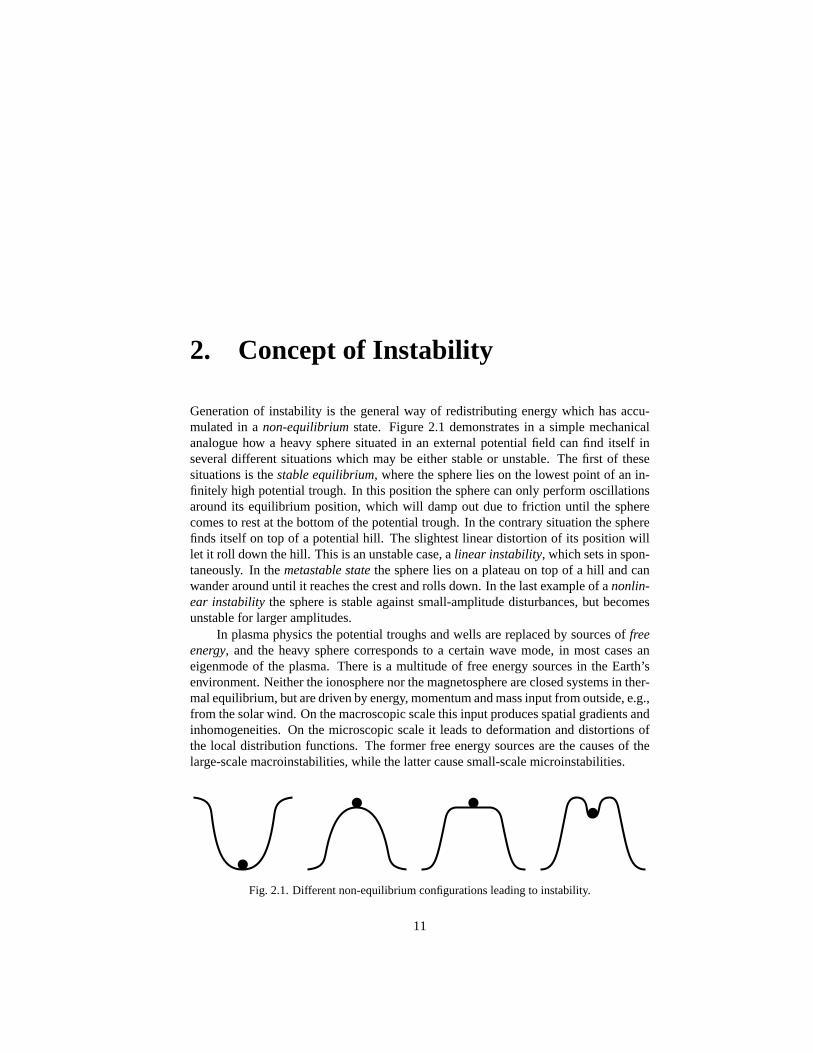
Generation of instability is the general way of redistributing energy which has accu-mulated in anon-equilibriumstate. Figure 2.1 demonstrates in a simple mechanicalanalogue how a heavy sphere situated in an external potential field can find itself inseveral different situations which may be either stable or unstable. The first of thesesituations is thestable equilibrium, where the sphere lies on the lowest point of an in-finitely high potential trough. In this position the sphere can only perform oscillationsaround its equilibrium position, which will damp out due to friction until the spherecomes to rest at the bottom of the potential trough. In the contrary situation the spherefinds itself on top of a potential hill. The slightest linear distortion of its position willlet it roll down the hill. This is an unstable case, alinear instability, which sets in spon-taneously. In themetastable statethe sphere lies on a plateau on top of a hill and canwander around until it reaches the crest and rolls down. In the last example of anonlin-ear instability the sphere is stable against small-amplitude disturbances, but becomesunstable for larger amplitudes.
In plasma physics the potential troughs and wells are replaced by sources offreeenergy, and the heavy sphere corresponds to a certain wave mode, in most cases aneigenmode of the plasma. There is a multitude of free energy sources in the Earth’senvironment. Neither the ionosphere nor the magnetosphere are closed systems in ther-mal equilibrium, but are driven by energy, momentum and mass input from outside, e.g.,from the solar wind. On the macroscopic scale this input produces spatial gradients andinhomogeneities. On the microscopic scale it leads to deformation and distortions ofthe local distribution functions. The former free energy sources are the causes of thelarge-scale macroinstabilities, while the latter cause small-scale microinstabilities.
Fig. 2.1. Different non-equilibrium configurations leading to instability.
11

12 2. CONCEPT OF INSTABILITY
2.1. Linear Instability
The concept of instability arises from a formal consideration of the wave function. Inlinear wave theory the amplitude of the waves is much less than the stationary statevector, so that the wave can be considered a small disturbance. For instance, if thewave is a disturbanceδn of the densityn, thenδn(x, t) ¿ n0, wheren0 can still bea function of space and time, but it is assumed that its variation is much slower thanthat of the disturbance. If this is the case, the wave function can be represented by asuperposition of plane waves oscillating at frequencyω(k), whereω is the solution ofthe linear dispersion relationD(ω,k) = 0. Any wave field componentδA(x, t) canthen be Fourier decomposed as
δA =∑
k
Ak exp(ik · x− iωt) (2.1)
In general the dispersion relation is a complex equation and has a number of frequencysolutions which are also complexω = ωr + iγ. From Eq. (2.1) it is clear that, forrealω, the disturbances are oscillating waves. On the other hand, for complex solutionsthe behaviour of the wave amplitude depends heavily on the sign of the imaginarypart of the frequencyγ(ωr,k). If γ < 0 the real part of the amplitude becomes anexponentially decreasing function of time, and the wave is damped. On the other hand,for γ > 0 the wave amplitude grows exponentially in time, and we encounter a linearinstability. In this case the decrementγ is called thegrowth rateof the correspondingeigenmode. Note, however, that instability can only arise if there are free energy sourcesin the plasma which feed the growing waves. If this is not the case, then a solution witha positiveγ is a fake solution which violates energy conservation and causality.
Growth Rate
The amplitude of an unstable wave increases as
Ak(t) = Ak exp[γ(ωr,k)t] (2.2)
Thus the linear approximation breaks down when the amplitude becomes comparableto the background value of the field, i.e.,Ak(t)/A0 ≈ 1, or at the nonlinear time
tnl ≈ γ−1 ln(
A0
Ak
)(2.3)
The linear approximation for unstable modes holds only for timest ¿ tnl. When thelinear approximation is violated, other processes set on which are called nonlinear be-cause they involve interaction of the waves with each other and with the backgroundplasma, which cannot be treated by linear methods. The timetnl is reached the earlier
2.1. LINEAR INSTABILITY 13
the larger the growth rate is. When the growth rate becomes larger than the wave fre-quency,γ > ω, the wave amplitude explodes and the wave has no time to perform evenone single oscillation during one wave period. The wave concept becomes obsoletein this case and it is reasonable to consider in the first place only instabilities of com-parably small growth rates which satisfy the conditions of linearity during many waveperiods
γ/ω ¿ 1 (2.4)
This remark does not preclude the existence of instabilities with growth rates largerthan the wave frequency. In fact, one of the first examples of an instability will dealwith this case below. One then speaks ofpurely growingor non-oscillatinginstabilitieswith about zero real frequency. Such instabilities appear only in the lowest frequencyrange of a magnetohydrodynamic plasma model.
Weak Instability
Instabilities can be either strong or weak. Strong instabilities have growth rates whichviolate the condition (2.4) and thus coincide in many cases with non-oscillating insta-bilities. For weakly growing instabilities with a growth rate satisfying Eq. (2.4), onecan design a general procedure to deduce the growth rate from the general dispersionrelation given in Eq. (I.9.55) of the companion book,Basic Space Plasma Physics. Thedispersion relation,D(ω,k)=0, is an implicit relation between the wave frequency andthe wavenumber. Given the wavenumber, it is possible to determine the wave frequency.In general,D(ω,k) is a complex function
D(ω,k) = Dr(ω,k) + iDi(ω,k) (2.5)
It therefore provides two equations which can be used to determine either the frequency,ω, in dependence on the wavenumber,k, or vice versa. It is convenient to assume thatk is real. Then the frequency is complex
ω(k) = ωr(k) + iγ(ωr,k) (2.6)
For growth rates satisfying Eq. (2.4) these expressions can be simplified by expandingD(ω,k) around the real part of the frequency,ωr, up to first order. This procedure,which is the same as used for calculating the damping rate in Sec. 10.6 of our compan-ion book,Basic Space Physics, yields
D(ω,k) = Dr(ωr,k) + (ω − ωr)∂Dr(ω,k)
∂ω
∣∣∣∣γ=0
+ iDi(ωr,k) = 0 (2.7)
Sinceω − ωr = iγ, this equation enables us to obtain a dispersion relation for the realpart of the frequency and at the same time an expression for the growth rate as
Dr(ωr,k) = 0 (2.8)
14 2. CONCEPT OF INSTABILITY
γ(ωr,k) = − Di(ωr,k)∂Dr(ω,k)/∂ω|γ=0
(2.9)
The first of these equations is the dispersion relation for real frequencies, while thesecond equation determines the linear growth rate,γ. In the following, as long as noconfusion is caused, we will drop the indexr, taking ω as the real frequency of thewave.
Spontaneous Cherenkov Emission
An illustrative example of wave amplification is the Cherenkov emission. We alreadyknow from Sec. 10.2 of the companion book,Basic Space Plasma Physics, that inverseLandau damping leads to amplification of plasma waves. This process depends onthe shape of the equilibrium distribution function. It is a process in which plasmawave emission is induced by the overpopulation of a higher level, very similar to Laseremission, and is calledinduced emission. Before we come to consider some of themost important plasma instabilities subject to this kind of induced emission, we pointout that there is also a different direct orspontaneous emissionmechanism, which isindependent of the overpopulation of the distribution function and also independent ofthe wave amplitude.
This kind of spontaneous emission is closely related to spontaneous emission ofelectromagnetic waves in a medium of large refraction index and therefore reduced lightvelocity,c′, from particles moving faster than the speed of light in the medium,ve > c′,theCherenkov effect. In a plasma the role of the light velocity is taken over by the phasevelocity of the plasma waves. There are many more than one possible wave modes ina plasma. Hence, spontaneous emission can appear in any of the plasma modes ifsome test particles exceed a certain critical velocity. For instance, if this velocity isthe reduced speed of light, the emission will be in the high-frequency electromagneticmodes. This requires high relativistic velocities of the particles. Since in a Maxwelliandistribution of a thermal plasma there are only very few such particles, this emission isnegligible. But emission in one of the electrostatic plasma modes is still possible. Sucha spontaneous emission occurs if fast test particles are in resonance with the plasmawave. In other words, the fast test particles, typically electrons, must have a velocitywhich is close to being equal to the phase velocity of the plasma wave
ve = ω(k)/k (2.10)
If we take the Langmuir wave, we haveω ≈ ωpe. This is very accurate because emis-sion of the waves by test particles can take place only for small
k2λ2D < 1 (2.11)
2.1. LINEAR INSTABILITY 15
corresponding to long wavelengths. Shorter wavelengths only contribute to the screen-ing of the particle in the Debye sphere. Both conditions together give the condition forspontaneous emission of Langmuir waves
ve = ωpe/k > ωpeλD = vth,e (2.12)
from fast electrons in a plasma. Hence, electrons with velocities faster than the electronthermal velocity contribute to spontaneous emission of Langmuir waves. This effectcan be understood from the expression for the total charge density variation
δρe(ω,k) =δρex(ω,k)
ε(ω,k)(2.13)
through the external charge fluctuation and the dielectric response function. Because ineach of the eigenmodes of the plasma the dielectric function vanishes,ε(ω,k) = 0, theplasma can still excite finite amplitude density fluctuations in the absence of externalfluctuations. In this case both the numerator and denominator of the above expres-sion vanish at the eigenmode yielding a finite charge fluctuation. This is the necessarycondition for spontaneous emission. If the plasma in addition contains particles whichsatisfy Eq. (2.12), it will spontaneously emit Langmuir waves. The rate of spontaneousemission is equal to the energy loss of the fast particles in the ‘collision’ with the long-wavelength eigenmodes. This energy loss of one single particle is
dWe
dt= −πmeω
4pe
2n0
∑
k
k−2 [δ(ω − k · ve) + δ(ω + k · ve)] (2.14)
The sum is over all wavenumbers satisfyingkλD < 1 and the two (not dimensionless!)delta functions account for the parallel and antiparallel resonant wave modes. Changingthe sign and integrating over the velocity distribution yields as a final result
(dWl
dt
)
Ch
=πmeω
4pe
2n0k2
∫d3v f0e(v)δ(ωpe − k · v) (2.15)
as spontaneous emission rate of Langmuir waves. Inserting a Maxwellian distributionof temperatureTe and carrying out the integration, one obtains for the emission rate
(dWl
dt
)
Ch
=4√
πωpekBTe
k5λ5D
(2.16)
in a thermal plasma in equilibrium. This emission is weak. In fact, it is proportional to(kλD)−5. Comparing this dependence with the(kλD)−3 dependence of Landau damp-ing, one recognizes that, for short wavelengths, Landau damping dominates over spon-taneous Cherenkov emission. This is the reason for the weakness of thermal Langmuir
16 2. CONCEPT OF INSTABILITY
fluctuations in the short-wavelength range. But for long wavelengths spontaneous emis-sion becomes stronger, and the Langmuir fluctuation level is relatively high. Clearly,if one adds a nonthermal component of higher velocity, for instance a beam of fastelectrons, the spontaneous emission rate is drastically enhanced.
2.2. Electron Stream Modes
Let us construct the simplest electrostatic dispersion relation leading to instability. Weconsider a cold plasma in order to dismiss any complications due to thermal effects.And we assume sufficiently high frequencies so that ion effects can be neglected. Toprovide a free-energy source we assume that a cold electron beam of densitynb andvelocityvb streams across the electron background of densityn0 and velocityv0 = 0.It is clear that this system is not at equilibrium and that the electrostatic interactionbetween the two plasmas should ultimately lead to dissipation of the extra energy storedin the streaming motion of the beam. The beam will be decelerated and the beamelectrons will mix into the background plasma. During this process the plasma will beheated. The ignition of this complicated process leading to thermodynamic equilibriumwill be caused by an instability.
Beam-Plasma Dispersion Relation
The dispersion relation of a beam-plasma system can be constructed by rememberingthat the plasma response function,ε(ω,k), is the sum of the contributions of the plasmacomponents. Since both components are cold and the plasma is isotropic, we get
ε(ω,k) = 1− ω2p0
ω2− ω2
pb
(ω − k · vb)2= 0 (2.17)
The first term on the right-hand side is the background plasma contribution which, inthe absence of the beam, would yield Langmuir oscillations. The second term is ofexactly the same structure, but with the background plasma frequency replaced by thebeam plasma frequency,ω2
pb = nbe2/ε0me, and the frequency being Doppler-shifted
by the beam velocity. Settingvb = 0, it is easily seen that the above dispersion relationreproduces Langmuir oscillations at the total plasma frequency,ω2
pe = ω2p0 + ω2
pb. Forvb 6= 0, Eq. (2.17) is a fourth-order equation in frequency,ω, which can have conjugatecomplex solutions, one of them with a positive imaginary part leading to instability, theother having a negative imaginary part and thus being damped and fading away in thelong-time limit.
If we neglect the background plasma by settingω2p0 = 0, the dispersion relation
can be solved for the streaming part, yielding
ω = k · vb ± ωpb (2.18)
2.2. ELECTRON STREAM MODES 17
low− ωhigh − ω
Uns
tabl
e
−kb kb 0 k
ωp0
ω
Langmuir
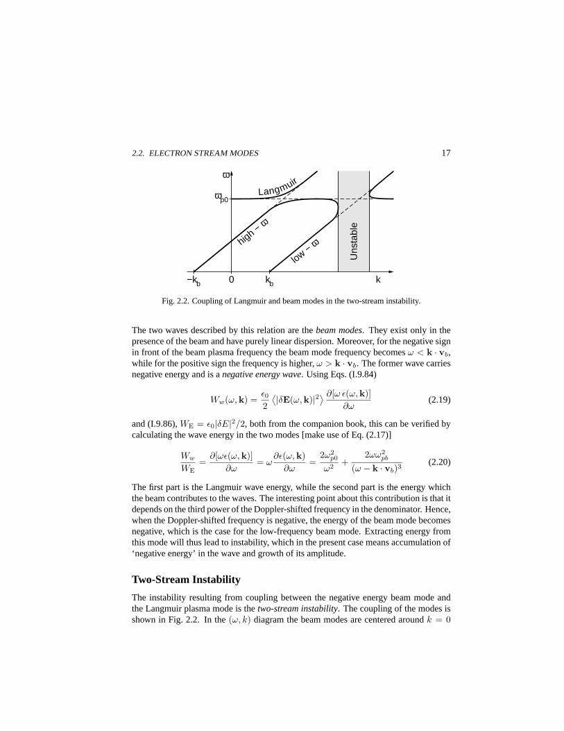
Fig. 2.2. Coupling of Langmuir and beam modes in the two-stream instability.
The two waves described by this relation are thebeam modes. They exist only in thepresence of the beam and have purely linear dispersion. Moreover, for the negative signin front of the beam plasma frequency the beam mode frequency becomesω < k · vb,while for the positive sign the frequency is higher,ω > k · vb. The former wave carriesnegative energy and is anegative energy wave. Using Eqs. (I.9.84)
Ww(ω,k) =ε02
⟨|δE(ω,k)|2⟩ ∂[ω ε(ω,k)]∂ω
(2.19)
and (I.9.86),WE = ε0|δE|2/2, both from the companion book, this can be verified bycalculating the wave energy in the two modes [make use of Eq. (2.17)]
Ww
WE=
∂[ωε(ω,k)]∂ω
= ω∂ε(ω,k)
∂ω=
2ω2p0
ω2+
2ωω2pb
(ω − k · vb)3(2.20)
The first part is the Langmuir wave energy, while the second part is the energy whichthe beam contributes to the waves. The interesting point about this contribution is that itdepends on the third power of the Doppler-shifted frequency in the denominator. Hence,when the Doppler-shifted frequency is negative, the energy of the beam mode becomesnegative, which is the case for the low-frequency beam mode. Extracting energy fromthis mode will thus lead to instability, which in the present case means accumulation of‘negative energy’ in the wave and growth of its amplitude.
Two-Stream Instability
The instability resulting from coupling between the negative energy beam mode andthe Langmuir plasma mode is thetwo-stream instability. The coupling of the modes isshown in Fig. 2.2. In the(ω, k) diagram the beam modes are centered aroundk = 0
18 2. CONCEPT OF INSTABILITY
with slopevb, while the Langmuir mode is a constant line atω = ωp0. Where the beammodes cross the Langmuir mode the dispersion curves couple together. At the low-frequency beam mode coupling point there is a region, where no real solution exists foreitherk or ω. This is the domain of conjugate complexity leading to instability.
In order to calculate the growth rate of the counterstreaming two-stream instability,the dispersion relation Eq. (2.17) must be rewritten as
1− ω2p0
ω2=
ω2pb
(ω − k · vb)2+
ω2pb
(ω + k · vb)2(2.21)
This equation has six roots of which the roots atω ≈ 0 andω ≈ ±k · vb are the mostinteresting. Puttingω = 0 on the right-hand side, the solution is
ω = ±ωp0k · vb/(k · v2b − 2ω2
pb)1/2 (2.22)
At short wavelengthsk · vb > 2ωpb this yields a real-frequency oscillation nearω <ωp0, valid for ωp0 small. At large wavelengths the dispersion relation has two purelyimaginary roots
ω = ±i√
2n0/nb (2.23)
one of them being unstable. The solution nearω ∼ k · vb satisfies the simplified dis-persion relation
1−( ωp0
k · v)2
=ω2
pb
(ω − k · vb)2+
ω2pb
4k · v2 (2.24)
Solving forω yields
ω = k · vb ± ωpbk · vb[k · v2
b − (ω2p0 + ω2
pb/4)]1/2
(2.25)
which for large values ofk · vb > ω2p0 + ω2
pb/4 is a real-frequency oscillation. At longwavelengths one, however, finds a conjugate complex solution
ωts = k · vb
1± iωpb(n0 + nb/4)−1/2
(2.26)
that yields one damped and one unstable mode. The latter has the growth rate
γts = ωpbk · vb/√
n0 (2.27)
Because the situation is symmetric, a similar instability is obtained for negative fre-quencyω ∼ −k · vb.
2.2. ELECTRON STREAM MODES 19
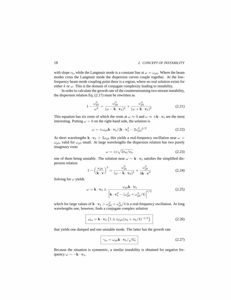
The graphical representation of the solution is shown in Figure 2.3 plotting thetwo sides of the two-stream dispersion relation Eq. (2.21) as two separate functions,εl
andεb, of frequency,ω. shows the principal shape of these functions.εl has a negativepole atω = 0 and approaches the horizontal line at 1 for large|ω|, while εb is alwayspositive, has poles atω = ±k · vb, vanishes for|ω| → ∞ and has a minimum atω = 0.The two crossing points outside the poles are the real high-frequency solutions of thedispersion relation. These are two of the six solutions of the dispersion relation. Theremaining solutions are conjugate-complex and correspond to low-frequency imaginarycrossings at frequencyω < kvb. One of these is the above unstable solution.
The two-stream instability is the simplest instability known. It is a cold electronfluid instability which in practice rarely occurs, because other kinetic instabilities set inbefore it can develop.
For a single cold beam in cold plasma the right-hand side of Eq. (2.21) containsonly one beam term. Nearω ≈ kvb this term is much larger than 1. In this case we get
ω2p0(ω − kvb)2 + ω2
pbω2 = 0 (2.28)
It is easily shown that it has the solutions
ω =kvb
2 + nb/n0
[1± i
(nb
n0
)1/2]
(2.29)
which yields an oscillation in the negative energy mode with a frequency just belowkvb
ωsb =kvb
2 + nb/n0(2.30)
and instability of this mode with growth rate
γsb = ωts
(nb
n0
)1/2
(2.31)
Weak Beam Instability
The two-stream instability is considerably modified when the beam density is much lessthan the density of the ambient plasma,nb ¿ n0. When this happens the Langmuirmode atω = −ωp0 decouples from the other solutions of the two-stream dispersionrelation. At this frequency the plasma behaves as if no beam exists. Decoupling of
20 2. CONCEPT OF INSTABILITY
1
−ωp0 ωp0 −kvb kvb ω
∋
∋
b
∋
b
∋
b ∋
b
∋
l
∋
l
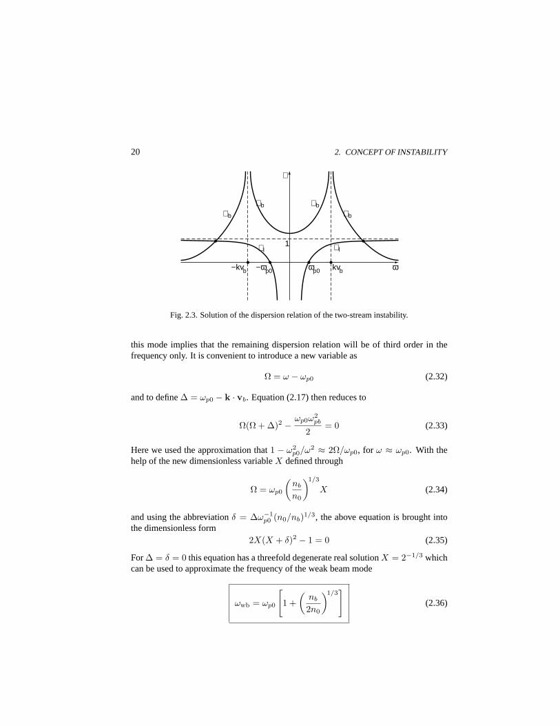
Fig. 2.3. Solution of the dispersion relation of the two-stream instability.
this mode implies that the remaining dispersion relation will be of third order in thefrequency only. It is convenient to introduce a new variable as
Ω = ω − ωp0 (2.32)
and to define∆ = ωp0 − k · vb. Equation (2.17) then reduces to
Ω(Ω + ∆)2 − ωp0ω2pb
2= 0 (2.33)
Here we used the approximation that1 − ω2p0/ω2 ≈ 2Ω/ωp0, for ω ≈ ωp0. With the
help of the new dimensionless variableX defined through
Ω = ωp0
(nb
n0
)1/3
X (2.34)
and using the abbreviationδ = ∆ω−1p0 (n0/nb)1/3, the above equation is brought into
the dimensionless form2X(X + δ)2 − 1 = 0 (2.35)
For∆ = δ = 0 this equation has a threefold degenerate real solutionX = 2−1/3 whichcan be used to approximate the frequency of the weak beam mode
ωwb = ωp0
[1 +
(nb
2n0
)1/3]
(2.36)
2.2. ELECTRON STREAM MODES 21
The growth rate of the unstable solution is found by insertingX = 2−1/3 + iγ into thethird-order equation forX. Solving for the imaginary part one finds thatγ2 = 3Ω2.This yields the growth rate of the weak beam instability
γwb =√
3ωp0
(nb
2n0
)1/3
(2.37)
This growth rate is much lower than that of the two-stream instability, because the freeenergy supplied by the weak beam is small. On the other hand, the instability is a high-frequency instability close to the background plasma frequency. Weak beams exciteLangmuir waves at small growth rates.
Stabilization and Quenching
The weak beam instability is the zero temperature limit of the more general hot beaminstability. One can show that a finite temperature will stabilize the weak beam insta-bility. The condition for instability was|ω − k · vb| ≈ ωp0(nb/2n0)1/3. If the beam isMaxwellian and has a thermal spread of1.4kvthb, Landau damping can be neglected aslong as|ω − k · vb| À 2vthb. On the other hand, the excited waves havek ≈ ωp0/vb.Combining these expressions, Landau damping can be neglected if
vthb
vb¿
(nb
n0
)1/3
¿ 1 (2.38)
Since the beam densities must be small, only relatively fast beams will cause weakbeam instabilities to grow. Otherwise the instability will make the transition to thetwo-stream instability. This is the case more relevant to space plasma physics, wheremost beams have sufficient time to relax and to become warm. But the initial stages ofbeam injection when narrow nearly monoenergetic beams leave from an accelerationsource as for instance auroral electric potential drops or electron beam reflection fromperpendicular shocks will lead to the weak beam instability.
One can estimate when the weak beam instability quenches itself. On p. 224 ofour companion book,Basic Space Physics, it was shown that for Langmuir waves abouthalf the energy is contained in the wave electric fluctuation while the other half is con-tained in the irregular thermal motion of the electrons. Hence, equatingWw/2 with thethermal energy of the beam electrons,Wthb = menbv
2thb/2, and using the threshold
condition in Eq. (2.38), one finds
Ww ≈ 2Wb
(nb
n0
)2/3
(2.39)
22 2. CONCEPT OF INSTABILITY
v0 v
f(v)
fi (v) fe(v)
0
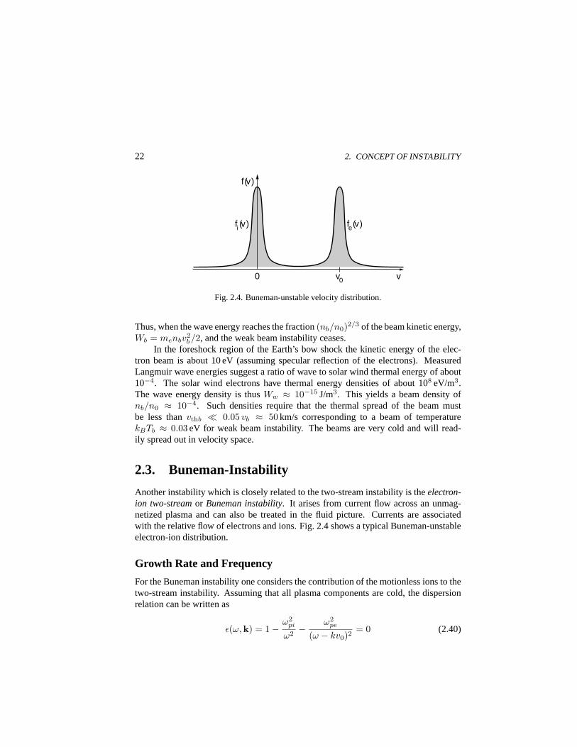
Fig. 2.4. Buneman-unstable velocity distribution.
Thus, when the wave energy reaches the fraction(nb/n0)2/3 of the beam kinetic energy,Wb = menbv
2b/2, and the weak beam instability ceases.
In the foreshock region of the Earth’s bow shock the kinetic energy of the elec-tron beam is about 10 eV (assuming specular reflection of the electrons). MeasuredLangmuir wave energies suggest a ratio of wave to solar wind thermal energy of about10−4. The solar wind electrons have thermal energy densities of about 108 eV/m3.The wave energy density is thusWw ≈ 10−15 J/m3. This yields a beam density ofnb/n0 ≈ 10−4. Such densities require that the thermal spread of the beam mustbe less thanvthb ¿ 0.05 vb ≈ 50 km/s corresponding to a beam of temperaturekBTb ≈ 0.03 eV for weak beam instability. The beams are very cold and will read-ily spread out in velocity space.
2.3. Buneman-Instability
Another instability which is closely related to the two-stream instability is theelectron-ion two-streamor Buneman instability. It arises from current flow across an unmag-netized plasma and can also be treated in the fluid picture. Currents are associatedwith the relative flow of electrons and ions. Fig. 2.4 shows a typical Buneman-unstableelectron-ion distribution.
Growth Rate and Frequency
For the Buneman instability one considers the contribution of the motionless ions to thetwo-stream instability. Assuming that all plasma components are cold, the dispersionrelation can be written as
ε(ω,k) = 1− ω2pi
ω2− ω2
pe
(ω − kv0)2= 0 (2.40)
2.3. BUNEMAN-INSTABILITY 23
Here the ions take over the position of the motionless component, while all electrons areassumed to stream across the ion fluid at their bulk velocity,v0. Clearly this will causea current to flow in the plasma. Because the ion plasma frequency is much smaller thanthe electron plasma frequency the dominating term is the electron term. Instability willarise at the slow negative energy mode
ωn ≈ kv0 − ωpe (2.41)
while the positive energy waveωp = kv0 + ωpe does not couple to the instability. Onecan thus rewrite the above relation as
(ω − ωn)ω2 =ω2
pi(ω − kv0)2
ω − ωp(2.42)
The wavenumber of interest isk ≈ ωpe/v0, because for a two-stream instability thiswavenumber couples to the negative energy wave. In contrast to the electron two-stream instability, the frequency is small compared to the electron plasma frequency,ω ¿ ωpe. With these approximations the dispersion relation becomes
ω3 ≈ − me
2miω3
pe (2.43)
Of the three roots of this equation one is a real negative frequency wave
ω = −(
me
2mi
)1/3
ωpe (2.44)
The other two are complex conjugate, and one of them has positive imaginary part. Tofind these two solutions we putω → ω + iγ to obtain the following two equations
ω(ω2 − 3γ2) = −meω3pe
2mi
γ2 = 3ω2(2.45)
The second equation givesγ = ±√3ω. Inserting into the first equation yields for thefrequency of the maximum unstable Buneman mode
ωbun =(
me
16mi
)1/3
ωpe ≈ 0.03 ωpe (2.46)
from which the growth rate is found to be
γbun =(
3me
16mi
)1/3
ωpe ≈ 0.05 ωpe (2.47)

24 2. CONCEPT OF INSTABILITY
kv0 ω
F(ω)
1
Real Solution
Com
plex
S
olut
ion
Real Solution
ωbun
Fig. 2.5. Graphical solution of the Buneman instability.
This growth rate is very large, of the order of the frequency itself. Hence, the Bunemaninstability is a strong instability driven by the fast bulk motion of all the electrons mov-ing across the plasma. One can expect that this instability will cause violent effects onthe current flow, retarding the current and feeding its energy into heating of the plasma.It is interesting to note that the Buneman two-stream waves propagate parallel to thecurrent flow but otherwise are electrostatic waves. As we will show later, they are thefast part of an ion-acoustic wave, which becomes unstable in weak current flow acrossa plasma.
Mechanism
To obtain an idea of the mechanism of the Buneman instability, we again use a graphicalrepresentation of the dispersion relation in the form
1 =ω2
pi
ω2+
ω2pe
(ω − kv0)2= F (ω) (2.48)
The functionF (ω) is shown in Fig. 2.5. It has two poles atω = 0 andω = kv0. Inbetween it has a minimum, whose position is found by calculating∂F (ω)/∂ω = 0
ωbun =kv0
1 + (mi/me)1/3(2.49)
Inserting this value intoF (ω) and demanding that the minimum ofF (ωbun) > 1, thecondition for instability is found to be
k2v20 < ω2
pe
[1 +
(me
mi
)1/3]3
(2.50)
2.3. BUNEMAN-INSTABILITY 25
Growth Rate
FrequencyT
hres
hold
1.0
0.5
0.5 1.0 1.5 ω2pe/k
2v0
2
1.0
0.5
γ/ω
bun
ω/ω
bun
Stable Unstable
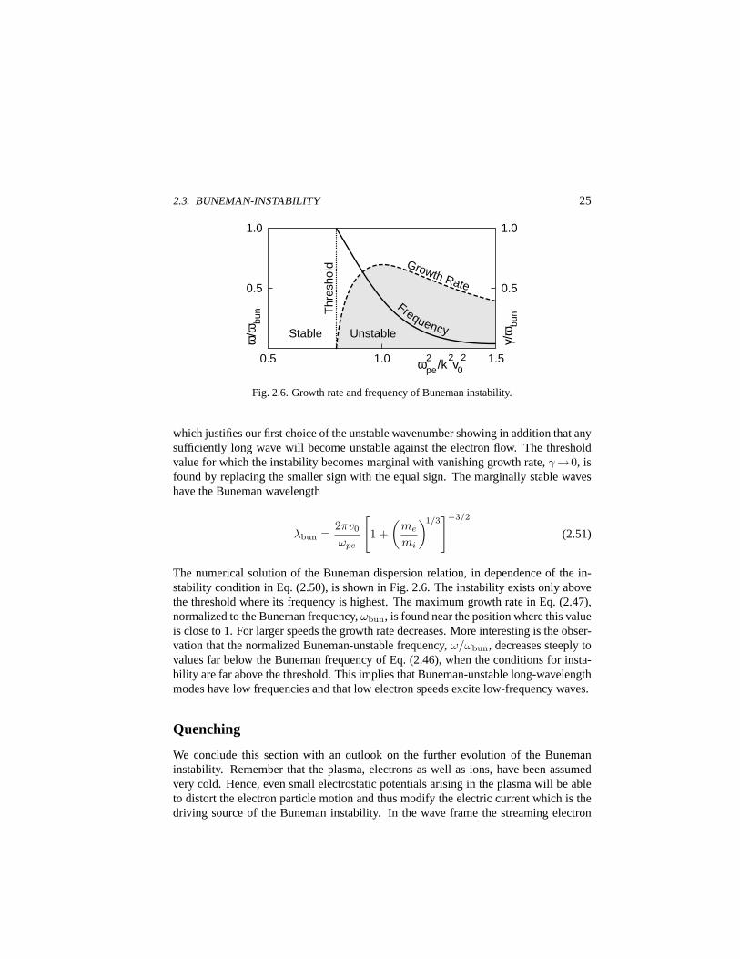
Fig. 2.6. Growth rate and frequency of Buneman instability.
which justifies our first choice of the unstable wavenumber showing in addition that anysufficiently long wave will become unstable against the electron flow. The thresholdvalue for which the instability becomes marginal with vanishing growth rate,γ→0, isfound by replacing the smaller sign with the equal sign. The marginally stable waveshave the Buneman wavelength
λbun =2πv0
ωpe
[1 +
(me
mi
)1/3]−3/2
(2.51)
The numerical solution of the Buneman dispersion relation, in dependence of the in-stability condition in Eq. (2.50), is shown in Fig. 2.6. The instability exists only abovethe threshold where its frequency is highest. The maximum growth rate in Eq. (2.47),normalized to the Buneman frequency,ωbun, is found near the position where this valueis close to 1. For larger speeds the growth rate decreases. More interesting is the obser-vation that the normalized Buneman-unstable frequency,ω/ωbun, decreases steeply tovalues far below the Buneman frequency of Eq. (2.46), when the conditions for insta-bility are far above the threshold. This implies that Buneman-unstable long-wavelengthmodes have low frequencies and that low electron speeds excite low-frequency waves.
Quenching
We conclude this section with an outlook on the further evolution of the Bunemaninstability. Remember that the plasma, electrons as well as ions, have been assumedvery cold. Hence, even small electrostatic potentials arising in the plasma will be ableto distort the electron particle motion and thus modify the electric current which is thedriving source of the Buneman instability. In the wave frame the streaming electron
26 2. CONCEPT OF INSTABILITY
energy is
We =me
2
(v0 − ωbun
kbun
)2
(2.52)
so that the condition for electron orbit distortion becomes
Ww(t) > nWe = 12nmev
20 (2.53)
where we took into account that the electrons move considerably faster than the wave.Now, the Buneman instability is a fast growing instability. The amplitude of the wavewill therefore quickly reach a sufficiently large value to trap the electrons and slowingthem down to the phase velocity of the wave which lies below threshold. The currentwill be disrupted in this case and the instability quenches itself. From the above con-dition we can estimate the time until quenching will happen, assuming that the waveamplitude grows from thermal level
Wtf ≈ kBTe/λ3D (2.54)
which was given in Eq. (I.9.27), as
WE(t) = Wtf exp(2γbunt) (2.55)
For the energy density we find from the Buneman dielectric response function
Ww(t) ≈(
16mi
me
)2/3
WE(t) (2.56)
For the thermal level we can assume that it is well approximated by the thermal levelof high-frequency Langmuir waves given in Eq. (2.54). Inserting all this into Eq. (2.53)and solving for the current disruption time,tcd, gives
ωpetcd ≈(
2mi
3me
)1/3
ln
[(me
16mi
)2/3v20
v2the
nλ3D
](2.57)
This expression depends only weakly on the electron current speed above threshold.The dominating number in the argument of the logarithm is the Debye number,ND =nλ3
D. Its logarithm is typically of the order of 15–30. Hence, in terms of the electronplasma frequency the self-disruption time of the current due to Buneman instability inan electron-proton plasma takes about 200 electron plasma periods or about 10 Bune-man oscillations. Thus the Buneman instability will manifest itself in spiky oscillationsof the current and in bursty emission of electrostatic waves below and up to the Bune-man frequency,ω < ωbun ≈ 0.03 ωpe.
2.4. ION BEAM INSTABILITY 27
2.4. Ion Beam Instability
As for a last introductory example we discuss an instability generated by two counter-streaming plasma flows, theelectrostatic streaming instabilityor counterstreaming ionbeam instability. It is important in many kinds of plasma flows as, for instance, the solarwind. Its electromagnetic counterpart plays a significant role in the foreshock region ofthe Earth’s bow shock.
Cold Electron Background
The dispersion relation of the counterstreaming ion beam instability including hot elec-trons consists of the two cold beam terms and a general hot electron term including theelectron plasma dispersion function
1− 12k2λ2
D
Z ′(
ω
kvthe
)− 1
2
[ω2
pi
(ω − kvb)2+
ω2pi
(ω + kvb)2
]= 0 (2.58)
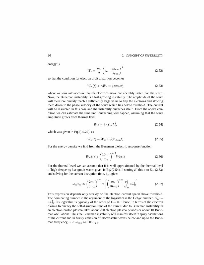
If the electrons are cold the distribution functions of the three components are wellseparated as shown in the left part of Fig. 2.7. The electron dispersion function reducesto ω2
pe/ω2, and the dispersion relation simplifies and can be written in a form similar tothe cold beam instability
1− ω2pe
ω2=
12
[ω2
pi
(ω − kvb)2+
ω2pi
(ω + kvb)2
](2.59)
Its graphical representation is given in Fig. 2.8. The dispersion relation has three polesat ω = 0,±kvb, and the functionF (ω) has two minima at low frequencies whichboth can be unstable. For sufficiently large beam velocities these minima are separatedfar enough to let the instability split into two Buneman-like instabilities, with growthrates given in the previous subsection, and one with positive, the other with negativefrequency.
v
vthe<<vb f(v)
fb (v) fe(v)
0 −vb vb
fb (v)
v
fe(v)
0 −vb vb
f(v)
fb (v) fb (v)
vthe≈vb
Fig. 2.7. Configuration of counterstreaming ion beam distributions.

28 2. CONCEPT OF INSTABILITY
−kvb kvb ω
Com
plex
S
olut
ion F(ω)
1
Real Solution
Com
plex
S
olut
ion
Real Solution
0
vthe<<vb
Fig. 2.8. Cold counterstreaming ion dispersion relation.
Hot Electron Background
On the other hand, when the electrons are hot (right-hand part of Fig. 2.7), we can usethe small argument expansion for the plasma dispersion function because for small fre-quenciesω/kvthe ¿ 1. Introducing the expansion given in App. A.7 of our companionbook, we write the dispersion relation as
1 +1
k2λ2D
=12
[ω2
pi
(ω − kvb)2+
ω2pi
(ω + kvb)2
](2.60)
Instead of Fig. 2.8 we now have Fig. 2.9. The horizontal line at1 + (kλD)−2 is theelectron contribution. The poles of the combined ion terms are atω = ±kvb. Thesolutions are the cross-overs of the ion function with the horizontal. There exist tworeal solutions at frequencies well outside the two poles. But at frequencies|ω| < kvb
real solutions are possible only for low ratiosωpi/kvb. Here the possibility for insta-bility arises. The instability is a low-frequency instability with frequencyω ≈ 0. Ina non-symmetric configuration with differing beam densities and beam velocities thesymmetry of the curves in Fig. 2.9 will be distorted, and the frequency will differ fromzero. The minimum atω = 0 has the valueω2
pi/k2v2b . Hence, instability sets in for
ω2pi
k2v2b
> 1 +1
k2λ2D
(2.61)
It can be satisfied for small beam velocities only. Thus the hot electrons quench thecounterstreaming ion beam instability.
Resonant Thermal Electrons
The instabilities discussed so far are instabilities where the whole plasma is involved.They are bulk ornon-resonantinstabilities. In the case of the counterstreaming ion
2.4. ION BEAM INSTABILITY 29
−kvb kvb ω
Unsta
ble
Sta
ble
ω2 pi
/k2 v b2
1+1/k2λD
2
vthe≈vb
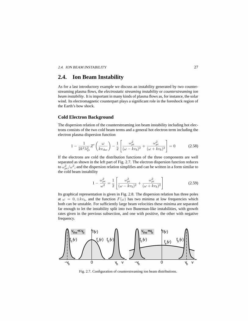
Fig. 2.9. Solution of the counterstreaming ion beam dispersion relation.
beam instability the quenching of the instability by the hot electron component appliesonly to the non-resonant instability. There is another range of frequencies, where thefrequency is of the order of the electron thermal velocity, implying resonant contribu-tion of electrons withv ≈ vthe ≈ ω/k. The frequency of this wave is still of the orderof the ion plasma frequency. Hence, their wavelength is very large compared with theDebye length. In this case the plasma dispersion function cannot be expanded and solu-tions are found only by numerical methods. The maximum growth rate of this resonantcounterstreaming ion beam instability in hot electron plasmas is considerably smallerthan the maximum Buneman growth rate
γib,max ≈ 0.1 γbun,max (2.62)
The small value ofγib,max is easily understood, because in contrast to the Bunemaninstability, where the whole plasma contributes, the counterstreaming ion beam insta-bility is fed by the small number of hot resonant electrons only. As a consequence thewaves cannot gain much energy. They are weakly growing waves and will cause muchless violent effects on the plasma than the ordinary Buneman instability.
Concluding Remarks
The present chapter introduces the reader to the concept of instability and explains thisconcept with a few illustrative examples. Although the concept of instability is math-ematically relatively simple, it presents a number of fundamental physical difficulties.Obtaining a positive imaginary part from a given dispersion relation does not neces-sarily imply that one really encounters an instability. Instabilities do arise only if free
30 2. CONCEPT OF INSTABILITY
energy is available. In other words, instabilities are physically real only when the statefrom which the instability starts is thermodynamically not in equilibrium. In a ther-modynamic equilibrium state, which offers no free energy, growing solutions of thedispersion relation are spurious and must be abandoned.
On the other hand, under thermodynamic non-equilibrium conditions instabili-ties are the most important effects. They cause all of the transitions a system expe-riences when changing from one state to another. In many cases they may cause theformation of new structure, while in other cases they lead to some kind of transitionalstate between total disorder and order, which is calledturbulence. Traditionally, non-equilibrium conditions are considered to be ordered states. This view is only partiallycorrect. Non-equilibrium states appear in the majority of cases only as transitionalstates between two different equilibrium configurations, where the structure is formedvia the onset of instability. Therefore, though instabilities act primarily to re-distributethe available free energy, they cause structure and order which may end up as anotherlong-living ordered equilibrium, which is very different from the most probable ther-modynamic equilibrium state.
Further Reading
Only a small selection of the many books on instabilities is given here. The general the-ory of instabilities is found in [5]. A useful introduction into a number of instabilities isgiven in [2]. Reference [3] contains a more or less systematic but not complete compila-tion of many instabilities which are to some extent relevant for space and astrophysics.Ion beam instabilities are completely reviewed in [4], electron beam instabilities in [1].
[1] R. J. Briggs,Electron-Stream Interaction with Plasmas(MIT Press, Cambridge,1964).
[2] A. Hasegawa,Plasma Instabilities and Nonlinear Effects(Springer Verlag, Heidel-berg, 1975).
[3] D. B. Melrose,Instabilities in Space and Laboratory Plasmas, (Cambridge Univer-sity Press, Cambridge, 1991).
[4] M. V. Nezlin, Physics of Intense Beams in Plasmas(Institute of Physics Publ.,Bristol, 1993).
[5] T. H. Stix,Waves in Plasma(American Institute of Physics, New York, 1992).
3. Macroinstabilities
Because of the multitude of free energy sources, a very large number of instabilities candevelop in a plasma. It is sometimes convenient to divide them into two large groupsaccording to the spatial scale involved in the instability. If this scale is of macroscopicsize, comparable to the bulk scales of the plasma, the instabilities are called macroinsta-bilities. On the other hand, if the characteristic size of the instabilities is microscopic,of the scale size of the particle inertial lengths and gyroradii, the instabilities are calledmicroinstabilities. In the latter case it is natural to assume that kinetic effects willbecome of greater importance than in the former case. Thus microinstabilities are typ-ically also kinetic instabilities while macroinstabilities can be treated in the frameworkof fluid plasma theory. In some cases, however, it is useful to account for kinetic ef-fects in macroinstabilities as well. The present section will cover the most importantmacroinstabilities appearing in space plasmas.
3.1. Rayleigh-Taylor Instability
On global scales plasma inhomogeneities cannot be neglected and several macroinsta-bilities are caused by plasma gradients. The simplest such instability is theRayleigh-Taylor instabilityor interchange instability. It is the instability of a plasma boundaryunder the influence of a gravitational field. Because of this reason it is also calledgravitational instability. Since the centrifugal force acts on a particle moving alongcurved magnetic field lines in a similar way as a gravitational force (see Sec. 2.4 of ourcompanion book,Basic Space Plasma Physics), this can lead to similar effects. Thisinstability is calledflute instability.
Mechanism
Consider a heavy plasma supported against the gravitational force by a magnetic fieldas shown in Fig. 3.1. The boundary between plasma and magnetic field is the horizontal(x, y) plane, and the magnetic field points in the direction ofx, so thatB0 = B0ex. Thegravitational accelerationg = −gez acts downward, while the plasma density gradient,
31

32 3. MACROINSTABILITIES
y
z
B0 g Vacuum Plasma
−δvEz
δvEz
−δEy
+δEy + + +
− − −
+ + +
− − −
Fig. 3.1. Rayleigh-Taylor unstable plasma configuration.
∇n0 = [∂n0(z)/∂z]ez points upward and
g · ∇n0 < 0 (3.1)
Let us for the moment neglect any thermal effects and assume that the plasma is colli-sionless. When the plasma boundary is distorted by a small purely electrostatic pertur-bation in the(x, y) plane, an instability can develop.
Consider a distortion of the boundary so that the plasma density makes a sinusoidalexcursion in thez direction. The gravitational field causes an ion drift and current inthe negativey direction,viy = −mig/eB0. The electrons, because of their negligiblemass, do not participate in this motion. Hence, in the region where the density distur-bance causes a density enhancement, below the boundary between plasma and vacuum,the ion motion leads to a charge separation and accumulation of positive charges asshown. As a result, a charge separation electric field,δEy, evolves. The horizontalelectric disturbance field in the+y direction,+δEy, causes an upward electric fielddrift, δvEz = +δEy/B0, in the external magnetic field while in the region of−δEy,the drift is downward,δvEz = −δEy/B0. These motions are in opposing directions;both of them amplify the initial distortion of the equilibrium density configuration atthe plasma-vacuum magnetic field boundary.
Hence, the dilutions of the plasma caused by the initial rarefaction begin to riseup into the plasma while the initial density increases below the boundary begin to falldown. This mechanism causes light dilute plasma bubbles to rise up into the denseplasma and, under the action of gravity, it causes plasma originally supported by themagnetic field to fall down into the plasma-free magnetic field region thereby eroding
3.1. RAYLEIGH-TAYLOR INSTABILITY 33
the boundary and causing loss of plasma. This is shown in the sequence of Fig. 3.1. Thebubbles themselves develop steep plasma boundaries which become unstable againstthe same Rayleigh-Taylor instability and deteriorate into smaller bubbles during thefurther evolution of the instability and the rise and fall of the bubbles. In the finalnonlinear stage of the instability the boundary will become diffuse and the wavelengthspectrum of the Rayleigh-Taylor mode becomes broadband, containing a wide range ofwavelengths reaching from the long initial one to the smallest possible scales.
Dispersion Relation
In order to quantify the discussion, we linearize the cold ion equation of motion includ-ing the gravitational force and introduce the plane wave ansatz for the ion velocity andthe electric field
δvi = δvi(ω,k) exp[i(k · x− ωt)]δE = −ikδφ(ω,k) exp[i(k · x− ωt)]
(3.2)
to obtain (ω +
gk⊥ωgi
)δvi⊥ =
e
mi(k⊥δφ− iB0ex × δvi⊥) (3.3)
Since the frequency of the disturbance will be much smaller than the ion gyrofrequency(ω′ ¿ ωgi) the solution for the velocity disturbance is
δvi⊥ = −δφ
[ik⊥ × ex +
k⊥ωgiB0
(ω +
gk⊥ωgi
)](3.4)
Using this equation to eliminate the velocity disturbance from the ion continuity equa-tion
ωδni = n0k · δvi − iδvi · ∇n0 (3.5)
one finds for the density disturbance
δni = n0δφ
[e
mi
(k2‖
ω2− k2
⊥ω2
gi
)+
k⊥B0Ln
(ω +
gk⊥ωgi
)−1]
(3.6)
We have introduced here the undisturbed inverse density gradient scale length
L−1n =
d lnn0(z)dz
> 0 (3.7)
Because the electrons are cold and do not drift in our model, the electron continuity andmomentum equations yield
δne = −δφn0
B0
(ωge
ω
k2‖
ω− k⊥
Lnω
)(3.8)
34 3. MACROINSTABILITIES
For these low-frequency variations one can safely assume that the condition of quasineu-trality, δne = δni, is satisfied. Inserting the expressions for the two oscillating densitiesleads to the dispersion relation
ωgi
ω
1k⊥Ln
(1− ω
ω + gk⊥/ωgi
)−
(1 +
mi
me
)ω2
gik2‖
ω2k2⊥
+ 1 = 0 (3.9)
This is a general dispersion relation for the Rayleigh-Taylor instability.
Growth Rate and Frequency
The highest growth rate of this instability is found for purely perpendicular propagationof the disturbance since in this case the electric field amplitude will lead to the largestvertical drift of the plasma for the longitudinal mode. Thus puttingk‖ = 0 and assuminga weak gravitational effect so thatω À k⊥g/ωgi, one can expand the term in bracketsin Eq. (3.9) to first order in this small parameter and obtains
ω2 = −g/Ln (3.10)
which has purely imaginary solutions and thus one purely growing solution with
γ0rt =(
g
Ln
)1/2
(3.11)
It is the same expression as found for fluids under the action of gravity.The non-oscillatory character of this instability results from the assumption of
smallk⊥g/ωgiω. Expanding up to second order in Eq. (3.9) yields
ω3 +g
Lnω − g2k⊥
2ωgiLn= 0 (3.12)
This equation has one real and two conjugate complex solutions. The unstable solutionhas frequency
ωrt = γ0rtcosh[
13cosh−1
(k⊥Lnγ0rt
2ωgi
)](3.13)
proportional to the zero-order growth rate,γ0rt. The corrected growth rate of this oscil-lating Rayleigh-Taylor mode is
γrt =√
3γ0rtsinh[
13cosh−1
(k⊥Lnγ0rt
2ωgi
)](3.14)
An approximate closed solution of Eq. (3.12) can be constructed for the complex fre-quencyω → ωrt + iγ. Separating the real and imaginary parts of Eq. (3.12) yields
3.1. RAYLEIGH-TAYLOR INSTABILITY 35
γ2 − 3ω2 = g/Ln
ω
(ω2 − 3γ2 +
g
Ln
)=
g2k⊥2ωgiLn
(3.15)
Together with Eq. (3.11) the first of these equations requires thatγrt À√
3ω, and thesecond equation gives for the frequency
ωrt = − gk⊥4ωgi
(3.16)
Consistency with the above condition demandsk⊥Ln ¿ 4ωgi(Ln/g)1/2, or in termsof the Rayleigh-Taylor wavelength
λrt
LnÀ π
2γ0rt
ωgi(3.17)
The right-hand side of this expression is small. So the condition of long wavelengths iseasily satisfied in all cases of interest.
For oblique propagation of the disturbance,k‖ 6= 0, part of the electric field isparallel to the magnetic field and can be short-circuited by the fast electron motion alongthe magnetic field thus causing a field-aligned current but at the same time partiallyquenches the instability. Let us write the dispersion relation for this case including thesecond term in Eq. (3.9)
ω2 = − g
Ln+
mi
me
k2‖
k2⊥
ω2gi (3.18)
When the condition
k‖k⊥
>
(me
mi
g
ω2giLn
)1/2
=(
me
mi
)1/2γ0rt
ωgi(3.19)
is satisfied, the right-hand side of this expression becomes positive, and the instabilityceases. Thus for a given density gradient scale,Ln, the last condition defines a marginalangle around the perpendicular direction. Inside this angle the Rayleigh-Taylor insta-bility can evolve. This angular range is very narrow, in the ionosphere typically lessthan one degree and the Rayleigh-Taylor mode is nearly-perpendicular here.
Magnetospheric Growth Rates
To obtain an idea of the magnitude of the growth rate of the Rayleigh-Taylor instabilityin the vicinity of the Earth, we introduce the gravitational accelerationg0(1RE) ≈
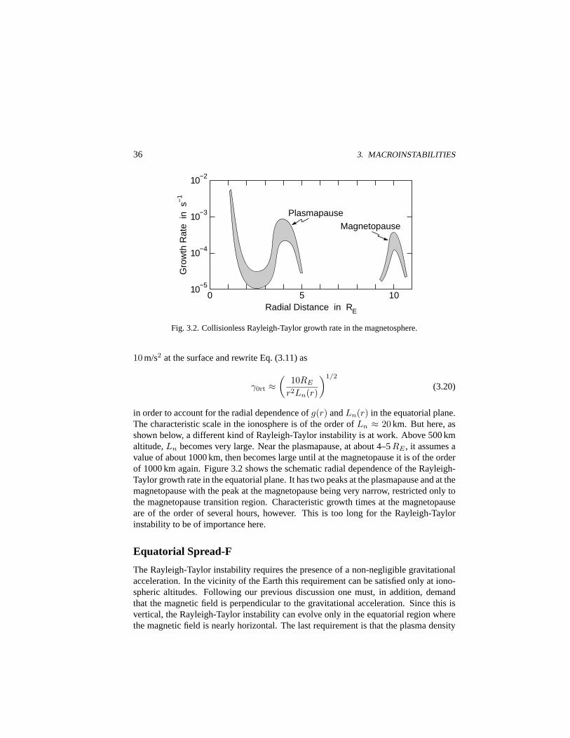
36 3. MACROINSTABILITIES
Plasmapause
Magnetopause
0 5 10
10−4
10−3
10−2
Radial Distance in RE
Gro
wth
Rat
e in
s−
1
10−5
Fig. 3.2. Collisionless Rayleigh-Taylor growth rate in the magnetosphere.
10 m/s2 at the surface and rewrite Eq. (3.11) as
γ0rt ≈(
10RE
r2Ln(r)
)1/2
(3.20)
in order to account for the radial dependence ofg(r) andLn(r) in the equatorial plane.The characteristic scale in the ionosphere is of the order ofLn ≈ 20 km. But here, asshown below, a different kind of Rayleigh-Taylor instability is at work. Above 500 kmaltitude,Ln becomes very large. Near the plasmapause, at about 4–5RE , it assumes avalue of about 1000 km, then becomes large until at the magnetopause it is of the orderof 1000 km again. Figure 3.2 shows the schematic radial dependence of the Rayleigh-Taylor growth rate in the equatorial plane. It has two peaks at the plasmapause and at themagnetopause with the peak at the magnetopause being very narrow, restricted only tothe magnetopause transition region. Characteristic growth times at the magnetopauseare of the order of several hours, however. This is too long for the Rayleigh-Taylorinstability to be of importance here.
Equatorial Spread-F
The Rayleigh-Taylor instability requires the presence of a non-negligible gravitationalacceleration. In the vicinity of the Earth this requirement can be satisfied only at iono-spheric altitudes. Following our previous discussion one must, in addition, demandthat the magnetic field is perpendicular to the gravitational acceleration. Since this isvertical, the Rayleigh-Taylor instability can evolve only in the equatorial region wherethe magnetic field is nearly horizontal. The last requirement is that the plasma density
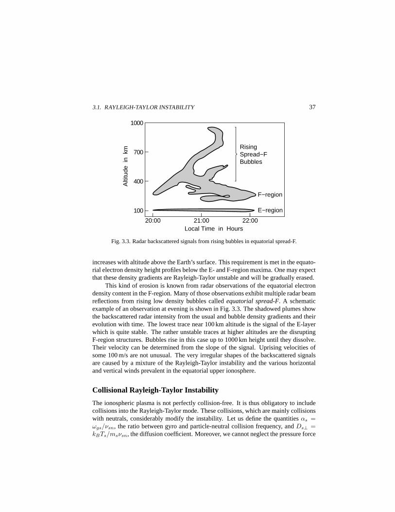
3.1. RAYLEIGH-TAYLOR INSTABILITY 37
20:00
100
Local Time in Hours
Alti
tude
in
km
400
700
1000
21:00 22:00
Rising Spread−F Bubbles
F−region
E−region
Fig. 3.3. Radar backscattered signals from rising bubbles in equatorial spread-F.
increases with altitude above the Earth’s surface. This requirement is met in the equato-rial electron density height profiles below the E- and F-region maxima. One may expectthat these density gradients are Rayleigh-Taylor unstable and will be gradually erased.
This kind of erosion is known from radar observations of the equatorial electrondensity content in the F-region. Many of those observations exhibit multiple radar beamreflections from rising low density bubbles calledequatorial spread-F. A schematicexample of an observation at evening is shown in Fig. 3.3. The shadowed plumes showthe backscattered radar intensity from the usual and bubble density gradients and theirevolution with time. The lowest trace near 100 km altitude is the signal of the E-layerwhich is quite stable. The rather unstable traces at higher altitudes are the disruptingF-region structures. Bubbles rise in this case up to 1000 km height until they dissolve.Their velocity can be determined from the slope of the signal. Uprising velocities ofsome 100 m/s are not unusual. The very irregular shapes of the backscattered signalsare caused by a mixture of the Rayleigh-Taylor instability and the various horizontaland vertical winds prevalent in the equatorial upper ionosphere.
Collisional Rayleigh-Taylor Instability
The ionospheric plasma is not perfectly collision-free. It is thus obligatory to includecollisions into the Rayleigh-Taylor mode. These collisions, which are mainly collisionswith neutrals, considerably modify the instability. Let us define the quantitiesαs =ωgs/νsn, the ratio between gyro and particle-neutral collision frequency, andDs⊥ =kBTs/msνsn, the diffusion coefficient. Moreover, we cannot neglect the pressure force
38 3. MACROINSTABILITIES
term in the fluid momentum equations. Solving the stationary momentum conservationequation for the particle velocity, we obtain
vs =Vs
1 + αs+
αs
1 + αsVs × B0
B0(3.21)
whereVs =
e
msνsnE +
gνsn
−Ds⊥∇ ln n (3.22)
For electrons the second term in Eq. (3.21) dominates becauseαe À 1. We thereforeneglect the first term in the electron velocity. Multiplying by the corresponding chargesand densities and subtracting ion and electron velocities yields for the current
j = σP E +en
ωgig × B0
B0− kB(Te + Ti)
B20
∇n×B0 (3.23)
whereσP is the Pedersen conductivity defined in Eq. (I.4.27) of our companion book.Due to their large mass the ions contribute most of the gravitational current permittingto approximate the plasma velocity by the ion velocity. Taking the divergence ofvi,assumingE0 = 0, we find
∇ · v = ∇ ·[g ×B0 +
kBTi
miB0 ×∇(ln n)
]= 0 (3.24)
which can be used on the right-hand side of the continuity equation
∂n
∂t+ v · ∇n = −n∇ · v = 0 (3.25)
Hence, the flow is practically incompressible. This approximation is very good for theF-region, but breaks down in the E-region. We linearize the continuity equation and theequation of vanishing current divergence
∇ · j = 0 (3.26)
using Eq. (3.23) forj. We further assume quasineutrality,ne = ni = n, for the low-frequency disturbances we expect and obtain
∇ · [(n0 + δn) (g ×B0 + νinδE)] = 0 (3.27)
This equation and the continuity equation together can be Fourier transformed. Intro-ducing the gradient scale length,Ln, and the electrostatic potential,δφ, the two trans-formed linear equations obtained are
3.1. RAYLEIGH-TAYLOR INSTABILITY 39
δn
n0+ i
k⊥νin
gB0δφ = 0
(ω
k⊥− g
ωgi
)δn
n0− 1
B0Lnδφ = 0
(3.28)
Solving this homogeneous system gives the dispersion relation of collision-dominatedRayleigh-Taylor modes in the equatorial ionosphere
ω =k⊥g
ωgi+ i
g
νinLn(3.29)
It is interesting that in this case a real part of the mode frequency appears naturally. Itsimply shows that the Rayleigh-Taylor mode propagates with phase velocity
ω
k⊥=
g
ωgi(3.30)
into perpendicular direction. This direction is easily found to be the eastward direction,g ×B0, in the equatorial ionosphere since the magnetic field points toward north andthe gravitational acceleration is vertically downward. The growth rate is this time givenby
γrtn =g
νinLn=
γ20rt
νin(3.31)
It depends on the collision frequency between ions and neutrals and is positive onlywhen the density gradient points upward.
The Rayleigh-Taylor instability in the ionosphere is clearly collision-dominated, asis obvious from its growth rate in Eq. (3.31). For vanishing collision frequency,νin→0,the growth rate would diverge. This non-physical behavior results from the approxima-tions made in the present theory. Actually, in a more elaborated theory which takes intoaccount the full particle dynamics and is not restricted to the fluid-drift approximation,one finds a smooth transition from the collisional to the collisionless Rayleigh-Taylorinstability. Formally this transition can be modelled as
γrt = γ0rt
[1− exp
(−γ0rt
νin
)](3.32)
a formula which describes both limits. In the limit of large collision frequency, the ex-ponential can be expanded and yields the growth rate in Eq. (3.31), while for vanishingcollisions the exponential dependence onνin disappears.
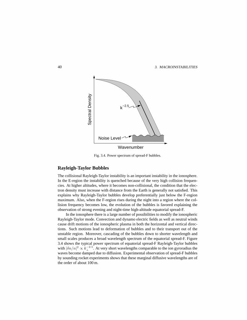
40 3. MACROINSTABILITIES
Wavenumber
Spe
ctra
l Den
sity
k−2.5
Noise Level
Fig. 3.4. Power spectrum of spread-F bubbles.
Rayleigh-Taylor Bubbles
The collisional Rayleigh-Taylor instability is an important instability in the ionosphere.In the E-region the instability is quenched because of the very high collision frequen-cies. At higher altitudes, where it becomes non-collisional, the condition that the elec-tron density must increase with distance from the Earth is generally not satisfied. Thisexplains why Rayleigh-Taylor bubbles develop preferentially just below the F-regionmaximum. Also, when the F-region rises during the night into a region where the col-lision frequency becomes low, the evolution of the bubbles is favored explaining theobservation of strong evening and night-time high-altitude equatorial spread-F.
In the ionosphere there is a large number of possibilities to modify the ionosphericRayleigh-Taylor mode. Convection and dynamo electric fields as well as neutral windscause drift motions of the ionospheric plasma in both the horizontal and vertical direc-tions. Such motions lead to deformation of bubbles and to their transport out of theunstable region. Moreover, cascading of the bubbles down to shorter wavelength andsmall scales produces a broad wavelength spectrum of the equatorial spread-F. Figure3.4 shows the typical power spectrum of equatorial spread-F Rayleigh-Taylor bubbleswith |δn/n|2 ∝ k−2.5
⊥ . At very short wavelengths comparable to the ion gyroradius thewaves become damped due to diffusion. Experimental observation of spread-F bubblesby sounding rocket experiments shows that these marginal diffusive wavelengths are ofthe order of about 100 m.
3.2. FARLEY-BUNEMAN INSTABILITY 41
3.2. Farley-Buneman Instability
Another instability is closely related to the ionospheric Rayleigh-Taylor instability. Itis also driven by transverse currents in the collisional ionosphere, but the nature of thecurrents is not gravitational. Rather these currents are drift currents, and the resultinginstability is amodified two-stream instabilityor Farley-Buneman instability. The in-stability arises from a difference in the drifts of electrons and ions forνin À ωgi (seeSec. 4.4 of our companion book).
Dispersion Relation
Let the electric field point vertically downward,E0 = −E0ez. In the crossed horizontalnorthward magnetic and vertical electric fields the electrons perform an eastwardE×Bdrift motion with a velocityvE = −E0/B0. The linearized and Fourier transformedelectron continuity equation yields for the disturbance of the electron velocity
δvey =(
ω
k⊥− vE
)δn
n0(3.33)
where quasineutrality has been assumed as usual for low-frequency waves. Neglectingelectron inertia and the action of gravity on the electrons but keeping electron-neutralcollisions we find after linearizing the electron equation of motion
ωgeδvey + νenδvez = 0
νenδvey − ωgeδvez = −ik⊥
(e
meδφ− kBTe
me
δn
n0
)(3.34)
Due to the high ion-neutral collision frequency ions do not move in the vertical direc-tion, viz ≈ 0, and the corresponding ion equations are
δviy − ω
k⊥
δn
n0= 0
(ω − iνin)δviy − k⊥v2thi
δn
n0=
e
mik⊥δφ
(3.35)
This linear homogeneous system of equations is solved by setting its determinant tozero, giving the dispersion relation
ω
(1 + iψ0
ω − iνin
νin
)= k⊥vE + iψ0
k2⊥c2
ia
νin(3.36)
42 3. MACROINSTABILITIES
The combined effect of electron and ion collisions and electron and ion gyrofrequenciesis contained in the quantity
ψ0 =νenνin
ωgeωgi=
νenνin
ω2lh
(3.37)
and the ion-acoustic speed is defined asc2ia = kB(Te + Ti)/mi. Electron and ion
gyration effects lead to the appearance of the lower-hybrid resonance frequency,ωlh, intheψ0-parameter.
Growth Rate and Frequency
As in the case of the Buneman instability the dispersion relation is a third-order equationin ω and can be solved in the same way. The weakly unstable solution yields for thefrequency
ωfb =k⊥vE
1 + ψ0(3.38)
and the growth rate
γfb =ψ0
νin
ω2fb − k2
⊥c2ia
1 + ψ0(3.39)
Buneman-Farley instability sets in whenever the wave phase velocity exceeds the ionacoustic speed,ωfb/k⊥ > cia or when the vertical drift velocity exceeds the threshold
vE > (1 + ψ0)cia (3.40)
Typical Altitude Range
This instability is of importance in the equatorial electrojet region, where large verticalelectric fields cause a strong horizontal drift current to flow above the equator. It letsbubbles rise into the current region and distorts the current flow in a way similar tothe Buneman instability. The parameterψ0 depends strongly on altitude. Recallingthe definition of the neutral collision frequency in Eq. (I.4.1) of our companion book,νsn = nnσn〈vs〉, one observes thatψ0 is proportional to the square of the neutral gasdensity. The latter satisfies the barometric law of Eq. (I.4.29),nn(z) = n0 exp(−z/H).
Hence,ψ0(z) decreases exponentially withz, as does the growth rate. The Farley-Buneman instability is thus restricted to lower altitudes. For a numerical value onehasψ0 ≈ 0.22 at z = 105 km. Assuming a scale height of 10 km, it readily becomessmall with altitude and can be neglected in Eqs. (3.38) and (3.39) abovez = 130 −150 km. The altitude range of the Farley-Buneman instability therefore is the equatorialE-region.
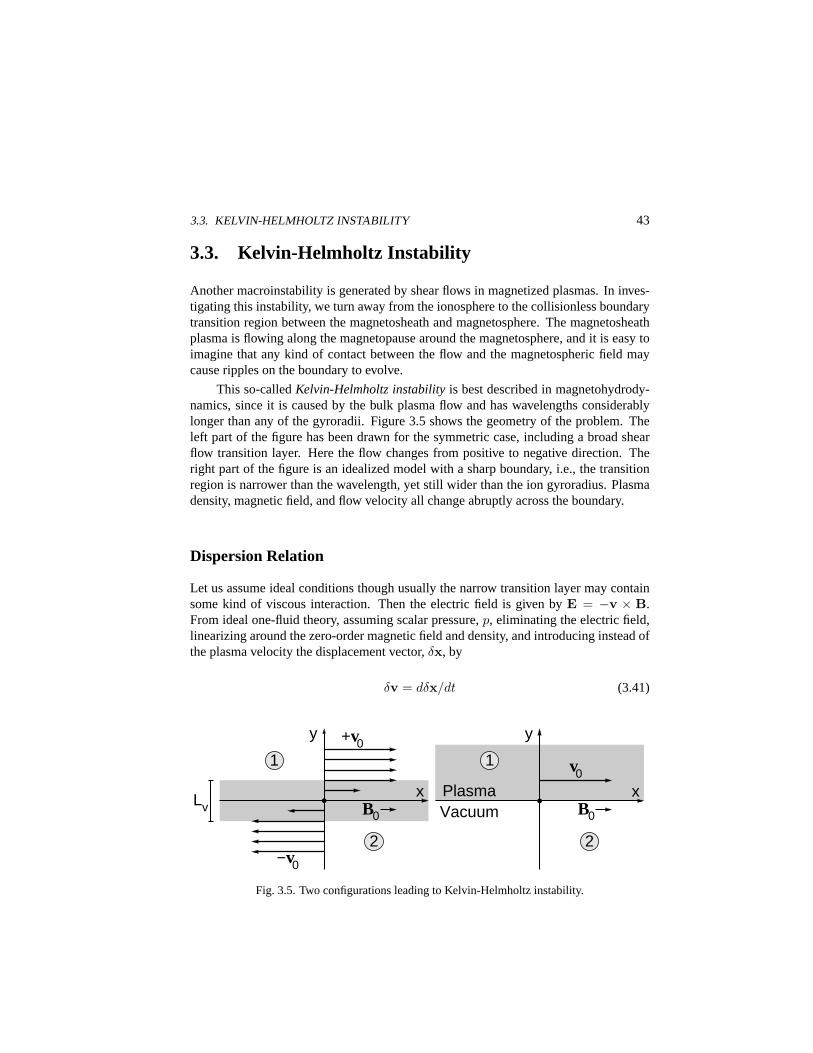
3.3. KELVIN-HELMHOLTZ INSTABILITY 43
3.3. Kelvin-Helmholtz Instability
Another macroinstability is generated by shear flows in magnetized plasmas. In inves-tigating this instability, we turn away from the ionosphere to the collisionless boundarytransition region between the magnetosheath and magnetosphere. The magnetosheathplasma is flowing along the magnetopause around the magnetosphere, and it is easy toimagine that any kind of contact between the flow and the magnetospheric field maycause ripples on the boundary to evolve.
This so-calledKelvin-Helmholtz instabilityis best described in magnetohydrody-namics, since it is caused by the bulk plasma flow and has wavelengths considerablylonger than any of the gyroradii. Figure 3.5 shows the geometry of the problem. Theleft part of the figure has been drawn for the symmetric case, including a broad shearflow transition layer. Here the flow changes from positive to negative direction. Theright part of the figure is an idealized model with a sharp boundary, i.e., the transitionregion is narrower than the wavelength, yet still wider than the ion gyroradius. Plasmadensity, magnetic field, and flow velocity all change abruptly across the boundary.
Dispersion Relation
Let us assume ideal conditions though usually the narrow transition layer may containsome kind of viscous interaction. Then the electric field is given byE = −v × B.From ideal one-fluid theory, assuming scalar pressure,p, eliminating the electric field,linearizing around the zero-order magnetic field and density, and introducing instead ofthe plasma velocity the displacement vector,δx, by
δv = dδx/dt (3.41)
+v0
−v0
1
2
Lv x
y
B0
v0
B0
x
y
Plasma Vacuum
1
2
Fig. 3.5. Two configurations leading to Kelvin-Helmholtz instability.
44 3. MACROINSTABILITIES
the linearized induction and momentum conservation equations can be written as
δB = ∇× (δx×B0) = B0 · ∇δx− δx · ∇B0 −B0∇ · δxµ0min0d
2δx/dt2 = −µ0∇δp− δB× (∇×B0)−B0 × (∇× δB)(3.42)
The induction law in the above version has been integrated with respect to timet. Wedefine the first order variation of the total pressure by
µ0δptot = µ0δp + B0 · δB (3.43)
EliminatingδB from the second Eq. (3.42), one obtains forδx
min0
[(vA · ∇)2 − ∂2
∂t2
]δx = ∇δptot + a (3.44)
We have introduced here the Alfven velocity,vA = B0/√
µ0min0, defined by thebackground parameters. The vectora on the right-hand side of this equation, whichresults from a combination of the vector operations in Eq. (3.42), is defined as
a = −δB · ∇B0 + B0 · ∇(B0∇ · δx + δx · ∇B0) (3.45)
Equation (3.44) shows the coupling of the Alfven wave on the left-hand side to the totalpressure disturbance on the right-hand side. Because the divergences of both the zero-order and the disturbed magnetic field components vanish,∇ · δB = ∇ ·B0 = 0, Eq.(3.42) can also be manipulated into an equation for the total pressure variation
∇2δptot = −mi∇ ·(
n0d2δxdt2
)+
1µ0∇ · (δB · ∇B0 + B0 · ∇δB) (3.46)
Now we assume that the plasma and the flow are homogeneous on both sides of the dis-continuity, so that total pressure balance is satisfied to all orders outside the boundary.This assumption implies that the perturbation is incompressible,∇·δv = 0. With theseassumptions the right-hand side of Eq. (3.46) vanishes, and the disturbance of the totalpressure satisfies
∇2δptot = 0 (3.47)
The only change inδptot occurs right at the infinitely thin boundary, while the pressuredisturbance fades with increasing distance from the boundary. This condition identifiesany possible linear disturbance as a surface wave. Another consequence of the assump-tion of homogeneity of the plasma outside the boundary is the vanishing of the vectora in Eq. (3.44). Equations (3.44) and (3.47), completed with the appropriate boundaryconditions at the discontinuity, form the basic linearized system of equations describingthe surface waves propagating along the boundary between the two media.
3.3. KELVIN-HELMHOLTZ INSTABILITY 45
The homogeneity of the problem along the interface between the two media allowsone to use a plane wave ansatz in the(x, z)-plane for both variables,δx andδptot, withhorizontal wavenumber,k = kxex + kzez, and frequencyω. From the equation for thedisplacement of the boundary one has
δx =∇δptot
min0 [ω2 − (k · vA)2](3.48)
and the variation of the pressure as solution of Eq. (3.47) is given by
δptot = p0 exp(−k|y|) exp[−i(ωt− kxx− kzz)] (3.49)
with k2 = k2x+k2
z . The exponentialy-dependence of this solution takes into account thedecay of the amplitude of the disturbance in the direction perpendicular to the interface.The physical reason behind this decay in an otherwise homogeneous medium is that theexcitation of the disturbance is located at the boundary between the two media, whereit must be largest. Outside the boundary the wave is evanescent, because no free energyis available there to further feed its amplitude.
The physical boundary conditions to be applied to the above solutions must alsoaccount for this fact. Hence, we choose that at a infinitely thin boundary the normalcomponent of the displacement,δxy, must be continuous. In addition total pressurebalance across the boundary is demanded, as is reasonable for a tangential disconti-nuity. Further, since the plasma parameters may change across the boundary we mustdistinguish the quantities to both sides by appropriate indices 1 and 2. Finally, in region1 the plasma streams with constant velocity,v0. This implies that the wave frequencyin region 1 will be Doppler-shifted toω1 = ω2 − k · v0, whereω2 = ω is the non-shifted frequency in region 2. Sinceδptot is continuous, the condition of continuity ofthe vertical component of the displacement yields
1n02 [ω2 − (k · vA2)2]
+1
n01 [(ω − k · v0)2 − (k · vA1)2]= 0 (3.50)
In deriving this equation one must take into account that the normals to both sides ofthe discontinuity are directed oppositely.
Equation (3.50) is the dispersion relation of the Kelvin-Helmholtz instability. For-mally this relation is very similar to the dispersion relations familiar from investigationof streaming instabilities. However, in the present case the role of the plasma modes istaken over by the two Alfven waves propagating in regions 1 and 2. Actually, the firstterm in Eq. (3.50) is the Alfven wave in the non-streaming region, while the secondterm is the Alfven wave in the streaming region as seen from region 2. The role of theinterface is merely to couple these two Alfven modes together. The Kelvin-Helmholtzinstability may therefore be identified as a streaming magnetohydrodynamic instability
46 3. MACROINSTABILITIES
which acts on Alfven waves. Of course, we have not distinguished between the dif-ferent species. Hence, it is no surprise that the dispersion relation obtained describessingle fluid waves. However, the above discussion shows that the Kelvin-Helmholtzinstability is one way to excite Alfven waves in a fluid by feeding surface waves fromextracting energy out of a shear flow along a boundary.
Frequency and Growth
Equation (3.50) is quadratic in frequency and yields an unstable solution
ωkh =n01k · v0
n01 + n02(3.51)
corresponding to the appearance of a conjugate complex root
(k · v0)2 >n01 + n02
n01n02
[n01(k · vA1)2 + n02(k · vA2)2
](3.52)
The Kelvin-Helmholtz instability thus occurs for a sufficiently large streaming veloc-ity in region 1. It is the relative streaming between the two plasmas on both sides ofthe thin boundary which drives the mode as a surface wave. Its frequency is that of aweighted beam mode with the geometric average of the two densities as weighting coef-ficient. Actually, the instability condition can be easiest satisfied for waves propagatingperpendicular to the unperturbed magnetic field. In the linear regime of the instabilitythe rigidity of the magnetic field provides the dominant restoring force, which sets athreshold on the instability.
Geomagnetic Pulsations
The Kelvin-Helmholtz instability is of considerable interest for the excitation of the ge-omagnetic pulsations discussed in Sec. 9.7 of our companion book. It is responsible forthe generation of surface wave modes at the magnetopause boundary by the fast tail-ward magnetosheath plasma flow along the magnetopause. The instability is restrictedto the boundary, but it is not localized to a certain position at the boundary. Ratherthe wave is convected tailward with the flow while its amplitude grows. Hence, largeamplitudes and consequently nonlinear behavior are expected only at the flanks of themagnetopause, while at the dayside magnetopause the amplitude of the surface wave isstill small. The surface undulation caused by it may then trigger resonances in the mag-netosphere which appear as pulsations. It is clear from the Kelvin-Helmholtz instabilitycondition that such pulsations will arise predominantly during cases of fast solar windor magnetosheath flows, and the faster the flow the shorter is the excited wavelength.

3.3. KELVIN-HELMHOLTZ INSTABILITY 47
KH−WaveKH−Wave
B0
Magnetopause
M’sheath Flo
wM
’sheath Flow
Fig. 3.6. Convective growth of magnetopause Kelvin-Helmholtz waves.
For the excitation of geomagnetic pulsations it is of interest to investigate the po-larization of the Kelvin-Helmholtz vortices inside the magnetosphere. Let us assumethat the wavenumber has only a very small component in thez direction. Then, fromthe condition of incompressibility,∇ · δx ≈ 0, we find that−kδxy + ikxδxx = 0.Hence, we obtain for the ratio
δxy
δxx=
ikx
(k2x + k2
z)1/2(3.53)
which shows that the Kelvin-Helmholtz waves are elliptically polarized in just the wayas used for the explanation of geomagnetic pulsations in Sec. 9.7 of our companionbook. Figure 3.6 shows a schematic of a Kelvin-Helmholtz wave flowing downtail andgrowing convectively during its propagation.
Kinetic Alfv en Waves
The dispersion relation of the Kelvin-Helmholtz instability, Eq. (3.50), contains the dis-persion relations of the Alfven waves on both sides of the transition layer. If we assumethat the transition layer is narrow, but that the variations along the boundary becomecomparable to the ion gyroradius, finite Larmor radius effects become important. TheAlfv en wave will then be replaced by the oblique kinetic Alfven wave (not by the shearAlfv en wave, sinceβ > me/mi at the magnetopause; see Fig. 10.12 of our companionvolume). The condition of instability for kinetic Kelvin-Helmholtz instability is still ofthe form of Eq. (3.52), but now with the kinetic Alfven velocity from Eq. (I.10.179)
48 3. MACROINSTABILITIES
vka‖ = vA
[1 + k2
⊥r2gi
(34
+Te
Ti
)]1/2
vka⊥ =k‖vA
k⊥
[1 + k2
⊥r2gi
(34
+Te
Ti
)]1/2 (3.54)
The field-aligned velocity of these waves is larger than that of the normal Alfven waves,but the velocity perpendicular to the field along the surface is reduced due to the smallratiok‖/k⊥. Correspondingly the kinetic surface wave excited by the Kelvin-Helmholtzinstability at the magnetopause not only propagates in the direction perpendicular toB0,but its speed is slow in this direction so that the instability has longer time to evolve. Inaddition, because for the kinetic Alfven wave the perpendicular wavenumber is largethe Doppler effect on the frequency in medium 1 is dominated byk⊥. Thus it is large forperpendicular convective flow so that the instability condition can be satisfied more eas-ily than in the ordinary Alfven case and the growth rate of the kinetic Kelvin-Helmholtzinstability will be larger than that of the ordinary instability.
Nonlinear Evolution
Application of the theory as given here to geomagnetic pulsations must be taken withcare. Some of the conditions set for our derivation of the Kelvin-Helmholtz instabil-ity are barely satisfied at the magnetopause. For instance, the magnetopause plasmais clearly not incompressible. Inclusion of compressibility complicates the problem,but does not suppress the instability entirely. However, the transition from the magne-tosheath to the magnetosphere has been found not to be steep. A broad boundary layerand plasma mantle is covering the magnetopause from its inner side. Here tangen-tial plasma flows have been frequently found, and density gradients are rather gradual.Hence, one must include gradual transitions in a calculation of the Kelvin-Helmholtzinstability.
Moreover, the magnetic field is not ideally tangential to the magnetopause. Nor-mal components caused by reconnection are the rule and violate the planar geometryassumption. Finally, dissipation must be included as well as the difference betweenelectron and ion dynamics, because the ion scales are comparable with the width of thetransition layer. Both have been neglected so far.
All these effects can be considered only in a more elaborated theory, coveringthe nonlinear evolution of the instability. Then the Kelvin-Helmholtz instability alsocontributes to plasma and momentum transport across the magnetopause by mixingof the two regions. When kinetic Alfven waves replace the magnetohydrodynamicwave mode at the magnetopause, parallel electric fields and field-aligned currents areproduced by the Kelvin-Helmholtz instability at the magnetopause, too.
3.3. KELVIN-HELMHOLTZ INSTABILITY 49
Auroral Kelvin-Helmholtz Instability
The Kelvin-Helmholtz instability may also occur in the upper auroral ionosphere. Herestrong shear flows have been observed near auroral arcs or bands. These shear flows areaccompanied by large perpendicular electric fields, which necessarily lead toE × Bflows of the upper ionospheric plasma. These flows are to good approximation hori-zontal in the nearly perpendicular auroral zone background magnetic field. Such shearflows, when exceeding the instability condition for Kelvin-Helmholtz instability, willcontribute to folding of the auroral structures. Here the incompressible approximationis quite reasonable because of the strong background magnetic field, but the existenceof field-aligned currents and the narrowness of the structures suggest that kinetic Alfvenwave are involved here. In this region the waves propagate in the shear kinetic Alfvenmode (see Sec. 10.6 of our companion book).
However, let us neglect all these effects, and just assume a negatively charged layerof auroral electrons with a width2d in the horizontalx direction, but of infinite extentalong the horizontaly and the verticalz axis. The magnetic field is, of course, alignedwith the vertical axis. Such a layer will cause strong shear flow along they axis due tothe polarization electric field directed toward the layer, parallel and antiparallel to thexaxis. Because the flow is caused by the electron charges and thus by a charge separationfield, this problem is fully electrostatic and can, outside of the charges, be described byLaplace’s equation
∇2δφ = 0 (3.55)
for the electric potential field disturbance,δφ. This disturbance is caused by the narrowcharge layer, which we consider as a charged surface. A wavelike disturbance of thepotential can be assumed as a surface undulation in the same way as for the conventionalKelvin-Helmholtz instability, this time for the potential field
δφ = δφ0 exp[±kx + i(ky − ωt)] (3.56)
The layer is uniform along the field, i.e., along thez axis, the wave amplitude decays inthe±x direction, and the wave propagates along they axis. The solution of Laplace’sequation in regions 1 and 2 and inside the layer,d, can be written as
δφ1(x, y)δφd(x, y)δφ2(x, y)
=
Aekx
Bekx + Ce−kx
De−kx
exp[i(ky − ωt)] (3.57)
The constants must be determined from the boundary conditions atx = ±d. Theseconditions are the continuity of the tangential electric field,δEy = −∂(δφ)/∂y, and therequirement that the jump in the normal electric field component,δEx, is the surfacecharge. The latter must be determined from the continuity equation for the electrons

50 3. MACROINSTABILITIES
under the condition that the flow is caused as a
δv = δE×B0/B20 (3.58)
motion in the undisturbed magnetic field. Clearly, the flow is incompressible and thelinearized continuity equation becomes
∂δn
∂t+ (v0·)∇δn = −(δv·)∇n0 (3.59)
The perturbation of the electron density at the boundaries,x = ±d, is calculated fromthe last two equations
δn
n0
∣∣∣∣±d
=δφ(±d)
B0(ω/k ∓ v0)∂ ln n0
∂x
∣∣∣∣±d
(3.60)
For sharp boundaries the derivative ofln n0 atx = ±d is discontinuous
∂ ln n0
∂x
∣∣∣∣±d
= δ(x + d)− δ(x− d) (3.61)
When we use this expression and multiply by the elementary charge we obtain thesurface charge,σs, which is the source of the electric field
σs(±d) = ±en0
B0
δφ
ω/k − v0(3.62)
The continuity ofδEy yields
A = B exp(2kd) + C
D = B + C exp(2kd)(3.63)
The discontinuity of the normal electric field component at the two surfaces gives
A + B exp(2kd)− C = σs(+d)/ε0
−D −B + C exp(2kd) = σs(−d)/ε0(3.64)
Combining the algebraic equations for the four coefficients and using the expressionsfor the surface charge densities we arrive at the dispersion relation
ω2 =ω4
pe
4ω2ge
[(1− 2ωgekv0
ω2pe
)2
− exp(−4kd)
](3.65)
which describes the evolution of Kelvin-Helmholtz waves in the auroral ionosphere un-der collisionless conditions, but in the presence of strong shear flows. The requirement
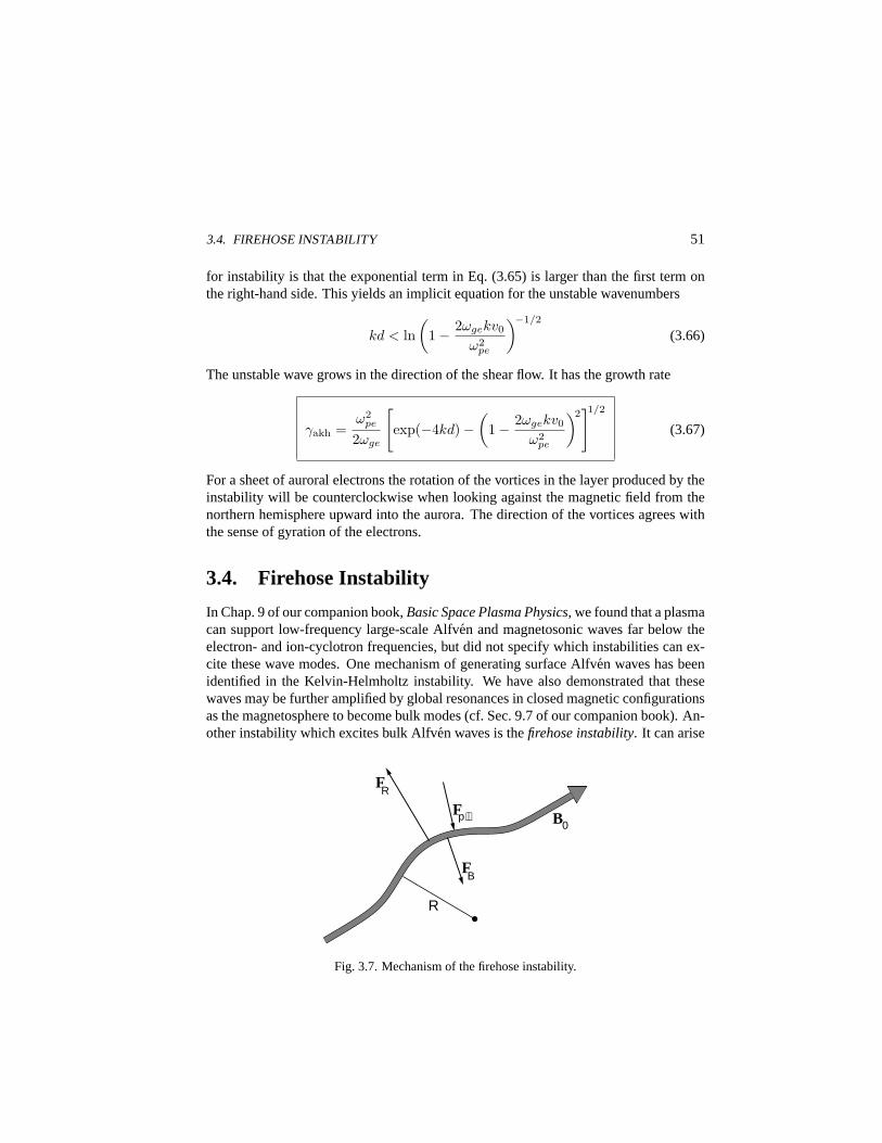
3.4. FIREHOSE INSTABILITY 51
for instability is that the exponential term in Eq. (3.65) is larger than the first term onthe right-hand side. This yields an implicit equation for the unstable wavenumbers
kd < ln(
1− 2ωgekv0
ω2pe
)−1/2
(3.66)
The unstable wave grows in the direction of the shear flow. It has the growth rate
γakh =ω2
pe
2ωge
[exp(−4kd)−
(1− 2ωgekv0
ω2pe
)2]1/2
(3.67)
For a sheet of auroral electrons the rotation of the vortices in the layer produced by theinstability will be counterclockwise when looking against the magnetic field from thenorthern hemisphere upward into the aurora. The direction of the vortices agrees withthe sense of gyration of the electrons.
3.4. Firehose Instability
In Chap. 9 of our companion book,Basic Space Plasma Physics, we found that a plasmacan support low-frequency large-scale Alfven and magnetosonic waves far below theelectron- and ion-cyclotron frequencies, but did not specify which instabilities can ex-cite these wave modes. One mechanism of generating surface Alfven waves has beenidentified in the Kelvin-Helmholtz instability. We have also demonstrated that thesewaves may be further amplified by global resonances in closed magnetic configurationsas the magnetosphere to become bulk modes (cf. Sec. 9.7 of our companion book). An-other instability which excites bulk Alfven waves is thefirehose instability. It can arise
FR
B0
FB
Fp⊥
R
Fig. 3.7. Mechanism of the firehose instability.
52 3. MACROINSTABILITIES
in a plasma when the plasma pressure becomes anisotropic. Then Eq. (I.7.21) from thecompanion book
P = p⊥I + (p‖ − p⊥)BBB2
(3.68)
holds. Under certain conditions a magnetic flux tube containing an anisotropic plasmacan be stimulated to perform global transverse oscillations similar to the oscillations ofa string brushed by a bow or of a firehose.
Mechanism
The physical mechanism of the firehose instability can be understood as follows. Imag-ine a magnetic flux tube and let the plasma flow along the magnetic field at averageparallel velocity〈v‖〉. As shown in Fig. 3.7, whenever a flux tube is slightly bent, theplasma will exert a centrifugal force,FR = min0v
2th‖/R, on the flux tube with curva-
ture radius,R.The centrifugal force is directed outward and tends to increase the amplitude of the
initial bending. In the absence of any restoring forces the flux tube would immediatelykink. However, the thermal pressure force in the plane perpendicular to the flux tube,Fp⊥, as well as the magnetic stresses of the flux tube,FB , resist the centrifugal force.Hence, instability sets in only for sufficiently large centrifugal forces or average parallelplasma velocities sufficiently large to overcome the restoring effects. Requiring forceequilibrium in the bending zone implies
min0v2th‖
R=
p⊥R
+B2
0
µ0R(3.69)
The terms on the left-hand side of this expression yield the parallel pressure forcep‖/R.Thus the condition for firehose instability is
p‖ > p⊥ + B20/µ0 (3.70)
Growth Rate
To derive the growth rate, we need the ideal magnetohydrodynamic equations (I.7.41)and (I.7.45), which forρE = 0 and together with Eq. (I.7.60) and the frozen-in condi-tion (I.7.54), all from the companion book, can be written as
∂n
∂t+∇ · (nv) = 0
∂(nmv)∂t
+∇ · (nmvv) = −∇ · P− 1µ0
B× (∇×B) (3.71)
∂B∂t
= ∇× (v ×B)

3.4. FIREHOSE INSTABILITY 53
together with the anisotropic equations of state from Eqs. (I.7.27) and (I.7.30), againfrom our companion book
d
dt
p⊥nB
= 0
d
dt
p‖p2⊥
n5= 0
(3.72)
Linearizing around an equilibrium state,n0, p0⊥, p0‖,B0,v0 = 0, and Fourier trans-forming, one obtains the dispersion relation
ω2 = 12k2v2
A
[A1 ± (A2
2 + A23)
1/2]
(3.73)
with
A1 = 12β0⊥(1 + sin2 θ) + β0‖ cos2 θ + 1
A2 = 12β0⊥(1 + sin2 θ)− 2β0‖ cos2 θ + 1 (3.74)
A3 = β0⊥ sin θ cos θ
whereθ is the angle betweenk andB0, andβ⊥0 = 2µ0p⊥0/B20 andβ0‖ = 2µ0p0‖/B2
0
are the parallel and perpendicular plasma beta parameters. When dividing both sides ofEq. (3.73) byk2, the right-hand side becomes independent ofk. Hence, the waves arenon-dispersive. It is easy to confirm that for propagation in the perpendicular direction,θ = 90, no instability can arise. For parallel propagation,θ = 0, we haveA3 = 0,and there are two solutions. One is purely real
ω2 = 3k2‖p0‖/n0mi (3.75)
and the stable parallel-propagating ion-acoustic wave. The other has a phase velocity
ω2
k2‖
= 12v2
A(β0⊥ + 2− β0‖) (3.76)
yielding instability under the condition (3.70), or in terms of parallel and perpendicularplasma beta
β0‖ > β0⊥ + 2 (3.77)
This is the condition for firehose instability which we derived above in Eq. (3.70) fromsimple physical considerations. Its growth rate is
γfh =k‖vA√
2(β0‖ − β0⊥ − 2)1/2 (3.78)
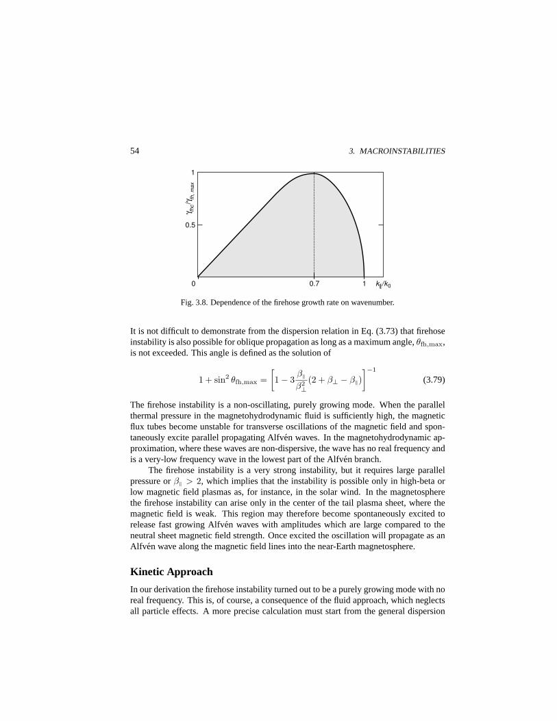
54 3. MACROINSTABILITIES
0 0.7 k||/k01
γ fhc/γ fh
, max
1
0.5
Fig. 3.8. Dependence of the firehose growth rate on wavenumber.
It is not difficult to demonstrate from the dispersion relation in Eq. (3.73) that firehoseinstability is also possible for oblique propagation as long as a maximum angle,θfh,max,is not exceeded. This angle is defined as the solution of
1 + sin2 θfh,max =[1− 3
β‖β2⊥
(2 + β⊥ − β‖)]−1
(3.79)
The firehose instability is a non-oscillating, purely growing mode. When the parallelthermal pressure in the magnetohydrodynamic fluid is sufficiently high, the magneticflux tubes become unstable for transverse oscillations of the magnetic field and spon-taneously excite parallel propagating Alfven waves. In the magnetohydrodynamic ap-proximation, where these waves are non-dispersive, the wave has no real frequency andis a very-low frequency wave in the lowest part of the Alfven branch.
The firehose instability is a very strong instability, but it requires large parallelpressure orβ‖ > 2, which implies that the instability is possible only in high-beta orlow magnetic field plasmas as, for instance, in the solar wind. In the magnetospherethe firehose instability can arise only in the center of the tail plasma sheet, where themagnetic field is weak. This region may therefore become spontaneously excited torelease fast growing Alfven waves with amplitudes which are large compared to theneutral sheet magnetic field strength. Once excited the oscillation will propagate as anAlfv en wave along the magnetic field lines into the near-Earth magnetosphere.
Kinetic Approach
In our derivation the firehose instability turned out to be a purely growing mode with noreal frequency. This is, of course, a consequence of the fluid approach, which neglectsall particle effects. A more precise calculation must start from the general dispersion
3.5. MIRROR INSTABILITY 55
relation for electromagnetic waves in the very-low frequency limit, using the magne-tized dielectric tensor in Eq. (I.10.147). The firehose mode is a solution of the left-handdispersion relation given in Eq. (I.10.156), including temperature anisotropy. If thisrelation is expanded up to second order ink‖vths/ωgs, i.e., in the ratio of gyroradius towavelength, the wave frequency retains a non-vanishing real part of the frequency
ωfh = γfhk‖/k0 (3.80)
whereγfh is the zero-order growth rate of the purely growing firehose mode obtainedabove from the fluid approach, and the wavenumberk0 describes a short wavelengthcut-off of the corrected growth rate
γfhc = γfh(1− k2‖/k2
0)1/2 (3.81)
which becomes effective when the wavelength of the firehose mode approaches the iongyroradius. This cut-off wavenumber is, for largeβ‖, given by
k20
4=
(γfh
k‖
)2(
1 +∑
s
ω2ps
ω2gs
)2 ∑s
ω2ps
ω3gs
[(γfh
k‖
)2
+(2Ts⊥ − 3Ts‖)
ms
]−2
(3.82)
The maximum growth rate is found at a wavenumberk‖ = k0/√
2, yielding for themaximum firehose growth rate
γfh,max = γfh
(k‖=k0/
√2)
/√
2 (3.83)
The oscillation is caused by the kinetic finite-gyroradius effect on the instability. Figure3.8 shows the dependence of the corrected growth rate on wavenumber. The modedisappears atk‖ > k0, above which it becomes heavily damped.
3.5. Mirror Instability
An instability complementary to the firehose instability is the so-calledmirror instabil-ity. It evolves at nearly perpendicular propagation of the waves. Though this instabilityis a macroinstability, affecting a large plasma volume and manifesting its effects on thelow-frequency scale in the macroscopic plasma parameters, it cannot be treated easilyin a magnetohydrodynamic model. The reason for this difficulty is that in this instabilitythe single particle motion along and perpendicular to the magnetic field must be takeninto account, which is not contained in the fluid picture of the plasma. One thereforeuses kinetic methods in the very-low frequency limit.
56 3. MACROINSTABILITIES
Dispersion Relation
The starting point is the kinetic dispersion relation of magnetized plasma waves in Eq.(I.10.147), which includes the temperature anisotropy,As, from Eq. (I.10.149), bothgiven in the companion book. For extremely low frequency modes,ω ¿ ωgi, withvery long wavelengths,krgi ¿ 1, these equations simplify. Because there is no bulkmotion of the particles, the tensor componentεs2 vanishes, and the dispersion relationwith k = k‖e‖ + k⊥ex splits into
N2‖ − εs1 = 0
(N2‖ + N2
⊥)−(
εs1 − εs0 +ε2s5εs3
)= 0
(3.84)
The first equation describes incompressible Alfven modes, including the anisotropyeffect and is thus the kinetic equivalent to the dispersion equation of the firehose mode.We note without proof that it can be brought into the form
ω2 = k2‖v
2A
[1− 1
2
∑s
(βs‖ − βs⊥)
](3.85)
which is the generalization of the firehose dispersion relation in Eq. (3.76) to two parti-cle species. As before, instability sets in when the right-hand side is negative.
The second dispersion relation describes compressible slow magnetosonic modes.In the low-frequency domain forεs3 À 1 it can be simplified. In this case the electronshave sufficient time during one oscillation to extinguish the ion-acoustic parallel electricwave field which is still coupled into the dispersion relation by the second term in thebrackets. Dropping this term we arrive at
(N2‖ + N2
⊥)− (εs1 − εs0) = (N2‖ + N2
⊥)− εyy = 0 (3.86)
as the dispersion relation for compressible modes. In explicit form and definingζs =ω/k‖vths‖ it reads
εyy =∑
s
ω2
ps
ω2gs
− N2‖
2
[βs⊥ − βs‖ + βs⊥
k2⊥
k2‖
(2 +
βs⊥βs‖
Z ′(ζs))]
(3.87)
Taking the very-low frequency limit and assuming that the phase velocities are small,ω/k‖vthi ∼ ω/kvA ¿ 1, we can simplify this relation even more by using the asymp-totic large argument expansion for the plasma dispersion function
i(π
2
)1/2 β2i⊥
βi‖
ω
k‖vthi‖= 1 +
∑s
(βs⊥ − β2
s⊥βs‖
)+
k2‖
k2⊥
[1 + 1
2
∑s
(βs⊥ − βs‖)
]
(3.88)

3.5. MIRROR INSTABILITY 57
δv||
δn |B|
Satellite Path
Fig. 3.9. Satellite measurements across a mirror-unstable region.
Only the ion component contributes to the imaginary part at these frequencies. Thefrequency of this mode is purely imaginary. It can be negative, in which case anymirror mode wave injected into the plasma will be quickly damped and will be unableto propagate. But if the bracketed term is negative, damping turns into growth.
Growth Rate
The mirror mode grows if the free energy of the pressure anisotropy is sufficiently largeand must be dissipated. A change in the sign ofω can be achieved in two ways. Whenwe assume that the waves propagate about parallel to the magnetic field,k2
‖ À k2⊥, the
second term in the brackets dominates, and the instability condition is∑
s
βs‖ > 2 +∑
s
βs⊥ (3.89)
which is the condition for firehose instability in Eq. (3.77). We have thus found that thefirehose mode can occur for compressible nearly-parallel propagating Alfven waves,too. This shows that any kind of Alfven waves will under the same condition of pressureanisotropy become unstable against firehose instability.
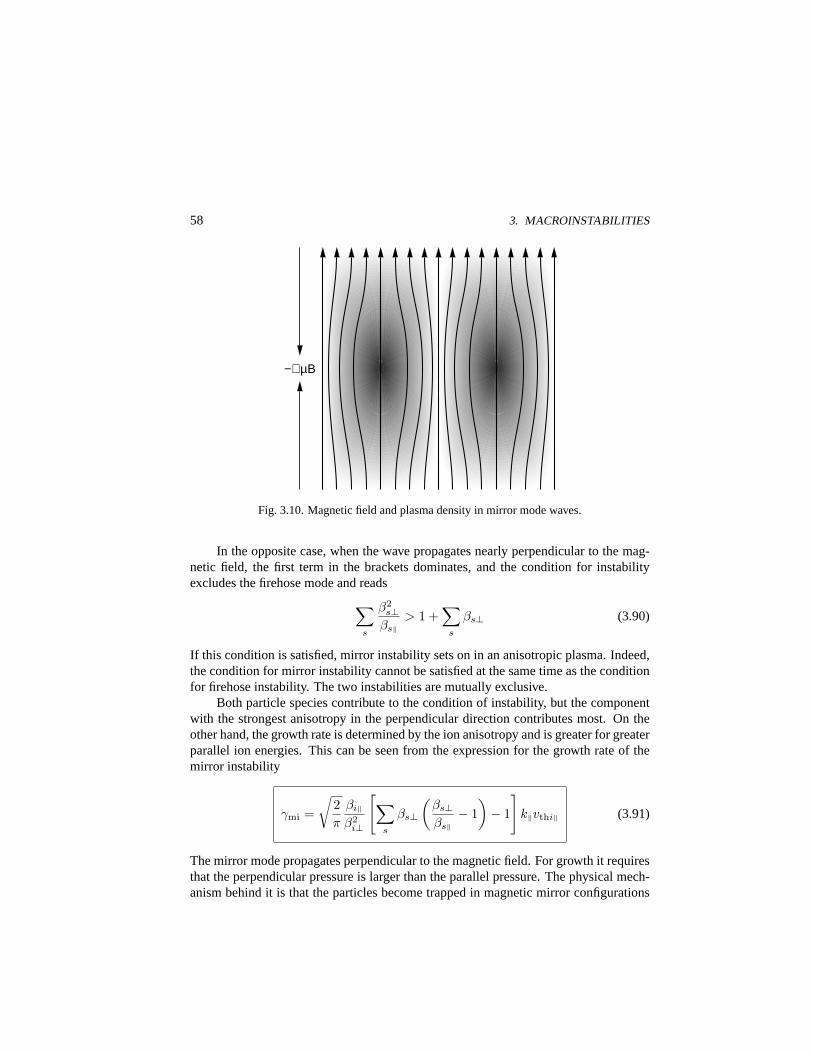
58 3. MACROINSTABILITIES
−∇µB
Fig. 3.10. Magnetic field and plasma density in mirror mode waves.
In the opposite case, when the wave propagates nearly perpendicular to the mag-netic field, the first term in the brackets dominates, and the condition for instabilityexcludes the firehose mode and reads
∑s
β2s⊥
βs‖> 1 +
∑s
βs⊥ (3.90)
If this condition is satisfied, mirror instability sets on in an anisotropic plasma. Indeed,the condition for mirror instability cannot be satisfied at the same time as the conditionfor firehose instability. The two instabilities are mutually exclusive.
Both particle species contribute to the condition of instability, but the componentwith the strongest anisotropy in the perpendicular direction contributes most. On theother hand, the growth rate is determined by the ion anisotropy and is greater for greaterparallel ion energies. This can be seen from the expression for the growth rate of themirror instability
γmi =
√2π
βi‖
β2i⊥
[∑s
βs⊥
(βs⊥βs‖
− 1)− 1
]k‖vthi‖ (3.91)
The mirror mode propagates perpendicular to the magnetic field. For growth it requiresthat the perpendicular pressure is larger than the parallel pressure. The physical mech-anism behind it is that the particles become trapped in magnetic mirror configurations
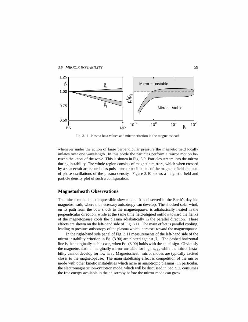
3.5. MIRROR INSTABILITY 59
MP BS
0.50
0.75
1.00
1.25
β⊥
β||
Mirror − unstable
β ⊥2 /β||
10−1 100 101 102 β⊥
Mirror − stable
β
Fig. 3.11. Plasma beta values and mirror criterion in the magnetosheath.
whenever under the action of large perpendicular pressure the magnetic field locallyinflates over one wavelength. In this bottle the particles perform a mirror motion be-tween the knots of the wave. This is shown in Fig. 3.9. Particles stream into the mirrorduring instability. The whole region consists of magnetic mirrors, which when crossedby a spacecraft are recorded as pulsations or oscillations of the magnetic field and out-of-phase oscillations of the plasma density. Figure 3.10 shows a magnetic field andparticle density plot of such a configuration.
Magnetosheath Observations
The mirror mode is a compressible slow mode. It is observed in the Earth’s daysidemagnetosheath, where the necessary anisotropy can develop. The shocked solar wind,on its path from the bow shock to the magnetopause, is adiabatically heated in theperpendicular direction, while at the same time field-aligned outflow toward the flanksof the magnetopause cools the plasma adiabatically in the parallel direction. Theseeffects are shown on the left-hand side of Fig. 3.11. The main effect is parallel cooling,leading to pressure anisotropy of the plasma which increases toward the magnetopause.
In the right-hand side panel of Fig. 3.11 measurements of the left-hand side of themirror instability criterion in Eq. (3.90) are plotted againstβ⊥. The dashed horizontalline is the marginally stable case, when Eq. (3.90) holds with the equal sign. Obviouslythe magnetosheath is marginally mirror-unstable for highβi⊥, while the mirror insta-bility cannot develop for lowβi⊥. Magnetosheath mirror modes are typically excitedcloser to the magnetopause. The main stabilizing effect is competition of the mirrormode with other kinetic instabilities which arise in anisotropic plasmas. In particular,the electromagnetic ion-cyclotron mode, which will be discussed in Sec. 5.2, consumesthe free energy available in the anisotropy before the mirror mode can grow.
60 3. MACROINSTABILITIES
3.6. Flux Tube Instabilities
The Kelvin-Helmholtz, the firehose, and the mirror instability are instabilities which aremagnetohydrodynamic in nature. We have discussed them in a different context becausethey do not push the magnetohydrodynamic viewpoint into the foreground. There is alarge number of instabilities which deserve the name magnetohydrodynamic with moreright. These modes evolve in laboratory magnetohydrodynamic devices and are relatedto resistive effects and plasma confinement. Few of these modes have relevance to spaceplasma physics. In the present section we are going to briefly discuss the foundations oftheir treatment and in the next section some flux tube instabilities of interest for spaceresearch will be analysed.
Magnetohydrodynamic stability depends on the inhomogeneity of the plasma, be-cause free energy in ideal magnetohydrodynamics can only be stored in inhomogeneousconfigurations. Good examples of such unstable situations aresolar flareswhich arebelieved to evolve in so-called active magnetic configurations, which evolve dynami-cally and possibly explosively. The instability of these magnetic configurations leadsto violent energy releases and causes the particle acceleration, matter ejection, opticalflashes, and the various radiation processes observed in the optical, radio, x- andγ-rayenergy ranges duringsolar flares. Another instability of magnetohydrodynamic natureis the reconnectionprocess, first introduced in Sec. 5.1 of our companion book. Tostudy these instabilities, it is convenient to formulate an energy principle. Such a prin-ciple is a global measure of the tendency of a magnetohydrodynamic configuration toundergo instability. In short, when the total energy variation turns out to be negative,one can expect the magnetohydrodynamic configuration to become unstable.
Energy Principle
Let us again introduce, as we have done in connection with the Kelvin-Helmholtz in-stability, the displacement vector,δx. The general form of the non-resistive linearizedmagnetohydrodynamic equations, except for the momentum equation, and integratedonce with respect to time is
δn = −∇ · (n0δx)δp = −δx · ∇p0 − γp0∇ · δx (3.92)
δB = ∇× (δx×B0)
Inserting these forms into the linearized momentum equation in Eq. (3.71), expressedin terms of the linear displacement gives
n0mid2δx/dt2 = δF(δx) (3.93)
3.6. FLUX TUBE INSTABILITIES 61
whereδF is defined as
µ0δF = −B0 × (∇× δB)− δB× (∇×B0) + µ0∇(δx · ∇p0 + γp0∇ · δx) (3.94)
The zero-order quantities are allowed to change in space. Since the above equations areall linear, it is convenient to eliminate the time dependence by Fourier transformationin time, yielding
n0miω2δx = −δF(δx) (3.95)
When we multiply this equation by the complex conjugate of the displacement vector,δx∗, and integrate over all space, we obtain
miω2
∫n0 |δx|2 d3x = −
∫δx∗ · δF(δx)d3x (3.96)
Subtract now the complex conjugate
miω∗2
∫n0 |δy|2 d3y = −
∫δy∗ · δF(δy)d3y (3.97)
from this equation. Clearly, the integrals over all space over different dummy variablesare the same. Thus one finds that the frequency is either real or purely imaginary,ω2 = ω∗2, which proves our previous finding that the Kelvin-Helmholtz, the firehoseand the mirror instability had only purely growing solutions. This is a general propertyof the magnetohydrodynamic equations.
To derive the energy principle, we multiply Eq. (3.93) by the displacement veloc-ity, δv = dδx/dt, and integrate over space
∫dδxdt
·[δF(δx)−min0(δx)
d2δxdt2
]d3x = 0 (3.98)
Becausen0(δx) and δF(δx) do not explicitly depend on time, this equation can betrivially integrated over time,t. We introduce the two quantities
∆W (δx, δx) = − 12
∫δx · δF(δx)
∆U(δx, δx) = 12mi
∫n0(δx) |δx|2 d3x
(3.99)
and can write the integrated equation as
∆W (δx, δx) + ∆U
(dδxdt
,dδxdt
)= const (3.100)
The constant on the right-hand side is the total displacement energy. Since this energyis unchanged and∆U ≥ 0, one immediately recognizes that the disturbance energy,
62 3. MACROINSTABILITIES
∆W , must be positive definite in order to guarantee the stability of the system, becauseonly then the mode cannot grow over the limitδU = 0. As a consequence of thisconclusion, we find in the opposite case that instability requires that
∆W (δx, δx) < 0 (3.101)
This is theenergy principlefor magnetohydrodynamic instability. The proof of its ne-cessity is a little more involved and can be found in the literature cited in the suggestionsfor further reading at the end of this chapter.
Energy Contributions
The energy variation,∆W , contains three contributions, the first is the plasma contri-bution,∆WP , provided by the integral over the plasma volume. The second,∆WA,comes from the surface integral over the plasma surface. The third is the vacuum con-tribution, ∆WV , which is the integral over all the outer space. This last contributionis
∆WV =1
2µ0
∫
>
|δBV |2 d3x (3.102)
with the integration over the outer volume of the plasma. Here one has to prescribeboundary conditions. These conditions are complicated. They are some form of theboundary conditions discussed in Chap. 8 of our companion book,Basic Space PlasmaPhysics, when one of the regions is assumed to be a vacuum. In space plasma physicswhen the plasma is assumed to be infinitely extended, the boundary is at infinity, andthe vacuum term can be dropped. But for finite systems, as for instance solar activeregions, it must be kept and introduces severe complications.
Similar arguments apply to the plasma surface contribution. It can be written as
∆WA = 12
∮
A
[∇
(p0 +
B20
2µ0
)]
A
· d(δF) |n · δx|2 (3.103)
wheren is the outer normal of the plasma volume and integration is over its surface.As in Chap. 8 of our companion book, the bracketed quantity here is the jump at thesurface. When surface currents are absent in equilibrium pressure equilibrium requiresthat this jump vanishes, and the integral is zero. This is the general case of an extendedplasma volume.
The most important contribution to the energy variation comes from∆WP
∆WP = 12
∫
P
d3x[µ−1
0 |δB|2 + γp0 |∇ · δx|2
+δx⊥ · ∇p0∇ · δx∗⊥ + δx∗ · (δB× j0)] (3.104)
3.6. FLUX TUBE INSTABILITIES 63
where the perpendicular and parallel direction refer to the equilibrium magnetic field.Introducing the unit vectore‖, the right-hand side of this formula can be written as
∆WP = 12
∫
P
d3x
µ−10 |δB⊥|2 + µ−1
0 |δB‖ − (δx⊥ · ∇p0)e‖/B0|2 + γp0 |∇ · δx|2
−(j0‖ · e‖)δB · (δx∗⊥ × e‖)− 2(δx⊥ · ∇p0) [(e‖ · ∇e‖) · δx∗] (3.105)
For instability to set in, the positive definite terms in this expression must be sufficientlysmall. The last of the positive terms can be eliminated by demanding that compress-ibility is small compared with the other terms. Then∇ · δx ≈ 0 can be neglected.Moreover,|δB|2 ' |B0 · ∇δx|2 is small and can be dropped whenever the radial gra-dients ofδx are much larger than the parallel variation of the displacement. This is truewhen field line bending can be neglected. Hence, one observes that instability occursfor large field-aligned current flow and for large perpendicular density gradients. Thesecond case is the case of interchange modes, the first is the case of kink modes.
Pinch Instability
There are three instabilities which are purely magnetohydrodynamic instabilities. Allof them are instabilities which can develop in a thin magnetic flux tube carrying alongitudinal current. These instabilities are thus caused by thej0-term in Eq. (3.105).These are the pinch, kink, and helical instabilities.
The physical picture of thepinch instabilityis that a field-aligned current in a fluxtube of radiusr produces its own azimuthal field,Bθ(r) ∝ 1/r, around the isolatedcurrent carrying flux tube. A slight distortion of the homogeneity of the flux tube alongits direction, as for instance a minor decrease in its radius and cross-section, will im-mediately cause an increase in this azimuthal field due to its1/r-dependence on theflux tube radius. This effect is self-amplifying and thus an instability. The final stateof this instability is that the current becomes pinched-off and is ultimately disrupted.Figure 3.12 shows the action of the pinch instability. The condition for instability of thepinch mode can be derived for a cylindrical straight flux tube assuming conservation ofmagnetic flux and current. It reads (without derivation)
B20θ ≈
(µ0I0
2πr
)2
> 2|B0‖|2 (3.106)
HereI0 is the current in the flux tube. Only strong currents can cause the pinch to de-velop. In the magnetosphere the pinch instability is probably of no importance becauseof the strong background magnetic field. But in solar coronal active regions extremelystrong field-aligned currents can evolve, which may become pinch-unstable, disrupt thecurrent, and change the magnetic field configuration.
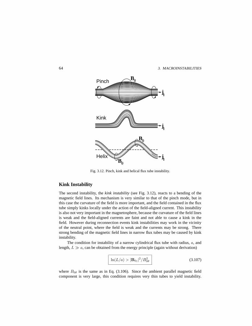
64 3. MACROINSTABILITIES
Bθ
j||
Pinch
j||
Kink
Bθ
Bθ
j||
Helix
Fig. 3.12. Pinch, kink and helical flux tube instability.
Kink Instability
The second instability, thekink instability (see Fig. 3.12), reacts to a bending of themagnetic field lines. Its mechanism is very similar to that of the pinch mode, but inthis case the curvature of the field is more important, and the field contained in the fluxtube simply kinks locally under the action of the field-aligned current. This instabilityis also not very important in the magnetosphere, because the curvature of the field linesis weak and the field-aligned currents are faint and not able to cause a kink in thefield. However during reconnection events kink instabilities may work in the vicinityof the neutral point, where the field is weak and the currents may be strong. Therestrong bending of the magnetic field lines in narrow flux tubes may be caused by kinkinstability.
The condition for instability of a narrow cylindrical flux tube with radius,a, andlength,L À a, can be obtained from the energy principle (again without derivation)
ln(L/a) > |B0‖|2/B20θ (3.107)
whereB0θ is the same as in Eq. (3.106). Since the ambient parallel magnetic fieldcomponent is very large, this condition requires very thin tubes to yield instability.
3.6. FLUX TUBE INSTABILITIES 65
Field-aligned currents in the inner auroral magnetosphere are unable to excite it, butagain in the solar corona or in the reconnection region of the tail kinking is not excluded.
Helical Instability
Thehelical instability(see Fig. 3.12) is very common in the solar corona. Its instabilitycondition is much lower than that of the other two so it will develop earlier if only astrong enough field-aligned current is flowing. Its effect is to transform a thin stretchedmagnetic flux tube into a spiral under the action of the self-magnetic effect of the field-aligned current. Flux tubes turn into helixes if it sets on. Such helical flux tubes havebeen observed in the x-ray light detected from the solar corona and emitted from hugesolar loops which have a twisted shape. The helical mode is unstable for
L/a > 2π|B0‖|/B0θ (3.108)
and is much easier to satisfy than the above two conditions. The latter condition favorslong flux tubes to become helically unstable. Remembering the definition ofB0θ thiscondition can be written
µ0I0L > 4π2a2|B0‖| = 4πΦ (3.109)
whereΦ is the constant magnetic flux inside the flux tube. Since the field-alignedcurrent strength inside the flux tube is constant, too, it is impossible to estimate at whatposition of the flux tube helical instability may set in.
As an example for this type of instabilities, let us outline the derivation of thedispersion equation for the helical mode. Assuming the magnetic field inside the tubeto be uniform, we find from Eq. (3.46) that the Laplace equation governs the evolutionof the total pressure disturbance
∇2δptot = 0 (3.110)
whereptot is the total internal pressure. The displacement vector is given by the sameexpression as for the Kelvin-Helmholtz instability
δx =∇δptot
min0(ω2 − k2v2A)
(3.111)
wherek is the azimuthal wave vector. In the region outside the flux tube the magneticdisturbance is a potential field,δBex = −∇ψ, with
∇2ψ = 0 (3.112)
66 3. MACROINSTABILITIES
because∇ × δBex = 0. These equations must be completed by boundary conditionswhich are relatively complex. One must impose pressure balance
ptot,in = (B0ex + δBex)2/2µ0 (3.113)
at the boundaryx = x0 + δxnn, wheren is the outer normal to the surface of theflux tube, andδxn is the normal displacement. One must also impose continuity of thetangential electric field
δEt = −(δv ×B0ex)t (3.114)
Linearizing the pressure condition for small displacements, one obtains
2µ0δptot = 2B0ex · δBex + δxn
[∂B2
0ex/∂n]
(3.115)
where the brackets again symbolize the jump. In cylindrical geometry this becomes
2µ0ptot = 2B0ex · δBex + δxn
(∂B2
0ex/∂n)
(3.116)
The condition on the electric field is rewritten using Faraday’s law
δBnex = n · ∇ × (δx×B0ex) (3.117)
We can solve these equations in a cylindrical geometry, taking into account the bound-ary conditions to determine the free constants when solving for the inner and outerregions. This procedure is standard and similar to the case of the Kelvin-Helmholtz in-stability, but complicated by the inhomogeneity and cylindric geometry of the problem.The dispersion relation ultimately obtained is
µ0min0ω2 = k2B2
0 +(
kB0‖ex +lB0θex
a
)2
− lB20θex
a2(3.118)
For the mode withl = 1 we find the unstable helical perturbation just under the condi-tion (3.108). This is the lowest wavenumber mode. Other modes with higher wavenum-bers may also exist but have higher thresholds as is immediately clear because to twistthe field more requires more energy and thus stronger currents.
In the magnetosphere the helical instability does not seem to occur. Since thecondition for instability is independent of the coordinate along the flux tube, we candiscuss numbers for ionospheric altitudes. At auroral latitudes, where the strongestfield-aligned currents are located, the magnetic field strength is|B0‖| ≈ 4 · 10−5 T.The length of a flux tube in a dipole field is about twice the equatorial distance fromthe center of the Earth,L = 2 LERE , and withLE ≈ 6 for the auroral zone, we getL ≈ 8 · 107 m. Using Eq. (3.109), we estimate that the field-aligned current density,j0 = I0/πa2, must be larger than 5µA/m2 for the onset of the helical instability. This
3.6. FLUX TUBE INSTABILITIES 67
value is about the same as the density of the strongest field-aligned current of cyclindri-cal geometry observed, i.e., the upward current connected to the head of the westwardtraveling surge (see Sec. 5.6 of our companion book). Hence, that current tube is onthe edge of instability. Possibly the helical instability limits the current to this uppervalue. However, there is no unambiguous observational evidence for the presence ofthe helical instability in the auroral zone. The probable reason for this is that in themagnetosphere a flux tube is surrounded by strong background field lines which, whenthe tube becomes distorted, start exerting strong forces onto the flux tube which coun-teract instability.
Flux tubes at the magnetopause have typical sizes ofa ≈ 103 km, fields of 100 nT,andL ≈ 20 RE . This suggests that field-aligned currents ofI0 > 3 ·104 A will becomeunstable against the helical instability. If such currents exist, instability should developat the outermost flux tube contacting the magnetosheath flow and should mix into theKelvin-Helmholtz instability. Since the flow stabilizes the mode, it should probablyevolve only in the vicinity of the stagnation point, where the flow velocity is low.
The helical instability also develops in the solar corona. Foot point field strengthsare of the order of 0.1 T, flux tube lengths between105 km and107 km, and foot pointdiameters of the order of104 km. Hence, currents of the order of1011 A will force theflux tube to twist. Since highly twisted flux tubes have frequently been observed, thecurrents in the solar corona may be strong enough to exceed the limit of stability.
Concluding Remarks
The overview of macroinstabilities given in the present chapter is not exhaustive. Itmerely provides a guide to the basic ideas. Macroinstabilities, because they deal withinhomogeneous plasmas, are usually rather difficult to treat even in the linear approxi-mation. They are important at large scales, when one needs to calculate the stability ofglobal plasma configurations. Such scales are common in astrophysical problems andin large fusion devices, where they cause violent changes in plasma configurations dur-ing instability like plasma disruptions. As a rule, macroinstabilities do affect the globalstructure of a plasma, e.g., the overall configuration of an active magnetic region onthe sun or that of the entire magnetosphere. Because of this reason they have attractedconsiderable interest in astrophysics and space physics. Macroinstabilities, because oftheir global properties and the inclusion of large-scale inhomogeneity into their treat-ment inevitably lead to the necessity of inclusion of boundary conditions. In addition tothe complication introduced by the boundary conditions, this is another property whichdistinguishes them from the wide field of microinstabilities treated in the next chapters.
68 3. MACROINSTABILITIES
Further Reading
Macroinstabilities are covered by [2] and [4]. For a general proof of the magnetohy-drodynamic energy principle for stability and instability see [1]. Here one also findsexplicit expressions for the vacuum-plasma boundary conditions and the theory of thecylindrical kink and helical modes. The theory of the mirror instability is given byHasegawa,Phys. Fluids, 12 (1969) 2642. For its nonlinear theory we have followedYoon,Phys. Fluids B, 4 (1992) 3627. Applications of macroinstabilities to solar physicsare given in [5] and [6]. Applications to the ionosphere can be found in [3], from wherewe have also taken the spread-F backscattered data. The measurements on which thedependences of the mirror criterion are based are found in Hill et al.,J. Geophys. Res.,100(1995) 9575.
[1] D. Biskamp, Nonlinear Magnetohydrodynamics(Cambridge University Press,Cambridge, 1993).
[2] A. Hasegawa,Plasma Instabilities and Nonlinear Effects(Springer Verlag, Heidel-berg, 1975).
[3] M. C. Kelley,The Earth’s Ionosphere(Academic Press, San Diego, 1989).
[4] D. B. Melrose,Instabilities in Space and Laboratory Plasmas, (Cambridge Univer-sity Press, Cambridge, 1991).
[5] E. Priest,Solar Magnetohydrodynamics(D. Reidel Publ. Co., Dordrecht, 1984).
[6] J. O. Stenflo,Solar Magnetic Fields(Kluwer Academic Publ., Dordrecht, 1994).
4. Electrostatic Instabilities
While macroinstabilities are caused by configuration space accumulations of free en-ergy in spatial inhomogeneities and affect the bulk or even global plasma properties,the effects of instabilities fed by velocity space inhomogeneities, i.e.,microinstabilities,are observed on smaller and sometimes microscopic scales. Free energy can be easilystored in deviations of the velocity distribution from its thermal equilibrium shape. Asa rule the equilibrium distributions are Maxwellian distribution functions (see Sec. 6.3of our companion book,Basic Space Plasma Physics). In an open system, like in spaceplasmas, a slight deformation of the Maxwellian distribution can be readily producedand there are many possibilities of such deviations from equilibrium. Correspondingly,a very large number of microinstabilities can arise in a plasma. The present chapterselects those which have been detected in space plasmas. We, however, restrict to elec-trostatic instabilities only leaving electromagnetic microinstabilities to the next chapter.Furthermore, we assume that the plasma is homogeneous which allows to neglect anyeffects caused by gradients and curvatures or by boundaries. The plasma is assumed tobe infinitely extended, and the source of free energy is taken to be invariable. The firstassumption is in many cases well satisfied because the typical scale of microinstabilitiesis small compared with the scales of the plasma. The second assumption, however, isvalid only over the short linear time scale of the instability, unless the source of freeenergy is maintained constant by external means. Usually for growing waves the in-stability quickly reaches the nonlinear stage and the free energy is diminished. Theseprocesses are inevitable but will be reserved for discussion in later chapters.
The starting point of a theory of linear microinstabilities is the linearized Vlasovequation
∂f
∂t+ v · ∇xf +
q
m(E + v ×B) · ∇vf = 0 (4.1)
or one of its derivatives introduced in Sec. 6.2 of our companion book, with the station-ary non-equilibrium distribution as ingredient. The procedure to obtain the dispersionrelation is the same as in Chap. 10 of the companion book. As in the case of macroin-stabilities, the dispersion relation must be solved for the frequency,ω, including itsimaginary part,γ. For weak instabilities the growth rate can be determined by usingthe methods developed in Sec. 2.1, since in these cases the growth rate yields only a
69
70 4. ELECTROSTATIC INSTABILITIES
small correction to the wave frequency and no new wave modes are introduced by thenon-equilibrium distribution functions. Instead, the free energy is used to excite one ofthe known kinetic plasma modes.
We will in most cases simply use the general dispersion relations from Eqs. (1.35)and (I.10.147), which are both derived in the companion volume, rewrite them for theparticular case, and model the unstable distribution as a combination of Maxwellians.For other non-thermal distributions analytical solutions do normally not exist.
4.1. Gentle Beam Instability
Electromagnetic waves may propagate from the outside into a plasma. In contrast,electrostatic waves cannot leave a plasma and cannot penetrate it. They must be excitedinternally. Since they are easily excited, they are the appropriate tool for the plasmato eliminate and redistribute the electric potential differences, which may arise dueto local charge separations, and to rearrange particles in the distribution function toachieve thermal equilibrium. These effects arise when the plasma is unmagnetized.They arise also when particle motion is allowed only along the magnetic field. In allsuch cases the kinetic electrostatic waves are excited by electrostatic instabilities.
Bump-in-Tail Distribution
The simplest kinetic instability is that of an electron beam propagating on a backgroundplasma. Figure 4.1 shows the phase space geometry of a beam plasma configurationcalledgentle beamor bump-in-tailconfiguration. The plasma is assumed thermal withfixed ions as neutralizing background and a certain electron temperature,Te, leading tothe thermal spread,vthe, of the background distribution function. Superposed on thisdistribution is a group of fast electrons at speedvb > vthe but much smaller densitythan the background plasma,nb ¿ n0, and of narrow thermal spread,vthb.
This phase space configuration is the classical case of a non-thermal distributionsubject to beam instability, but since we permit for finite beam temperatures, corre-sponding to deformation of the equilibrium distribution function, the instability willaffect only that part of the distribution function which contains the deviation from ther-mal equilibrium, while the bulk distribution remains unchanged. To treat this kind ofinstability we must go from the fluid to a kinetic treatment.
Inverse Landau Damping
A system consisting only of electrons will be subject to Langmuir oscillations or, whenincluding thermal effects, to propagating Langmuir waves with a dispersion given by
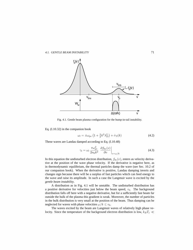
4.1. GENTLE BEAM INSTABILITY 71
vthb fb(v)
fe(v)
vthe vb v
∆(ω/k)
Ww
v
Fig. 4.1. Gentle beam plasma configuration for the bump-in-tail instability.
Eq. (I.10.32) in the companion book
ωl = ±ωpe
(1 + 3
2k2λ2D
)+ iγl(k) (4.2)
These waves are Landau damped according to Eq. (I.10.48)
γl = ωl
πω2pe
2n0k2
∂f0e(v)∂v
∣∣∣∣v=ω/k
(4.3)
In this equation the undisturbed electron distribution,f0e(v), enters as velocity deriva-tive at the position of the wave phase velocity. If the derivative is negative here, asin thermodynamic equilibrium, the thermal particles damp the wave (see Sec. 10.2 ofour companion book). When the derivative is positive, Landau damping inverts andchanges sign because there will be a surplus of fast particles which can feed energy tothe wave and raise its amplitude. In such a case the Langmuir wave is excited by thegentle beam instability.
A distribution as in Fig. 4.1 will be unstable. The undisturbed distribution hasa positive derivative for velocities just below the beam speed,vb. The backgrounddistribution falls off here with a negative derivative, but for a sufficiently fast beam faroutside the bulk of the plasma this gradient is weak. Moreover, the number of particlesin the bulk distribution is very small at the position of the beam. Thus damping can beneglected for waves with phase velocitiesω/k ≤ vb.
The waves excited by the beam are Langmuir waves of relatively high phase ve-locity. Since the temperature of the background electron distribution is low,kBTe ¿

72 4. ELECTROSTATIC INSTABILITIES
Wb = mev2b/2, the frequency of the waves will be close to the background plasma
frequency,ω ≈ ωpe. The condition of resonance,ω ≈ kvb, then requires that thewavenumber is small. Langmuir waves driven unstable by the beam will have longwavelengths.
Growth Rate
To calculate the growth rate of gentle beam excited Langmuir waves we consider aone-dimensional case, where the distribution function is the sum of two Maxwellians
f0e(v) = f0(v) + fb(v − vb) (4.4)
wheref0(v) is the Maxwellian background distribution, andfb(v − vb) is a shiftedMaxwellian. The dielectric function of the combined distribution is
ε(ω, k) = 1− ω2p0
ω2
(1 + 3k2λ2
D0
)− πiω2
p0
n0k2
∂f0(v)∂v
∣∣∣∣v=ω/k
− ω2pb
ω2
(1 + 3k2λ2
Db
)− πiω2
pb
nbk2
∂fb(v − vb)∂v
∣∣∣∣v=ω/k
(4.5)
If the beam density and temperature are low, the beam contribution to the real part of thedispersion relation can be neglected. The real part ofε yields the bulk plasma Langmuirwave dispersion relation,ω2
l = ω2p0(1+3k2λ2
D0). The weak beam causes a weak beaminstability. Thus we apply Eq. (2.9) to calculate the growth rate. The derivative of thereal part ofε(ωl, k) with respect toωl gives
∂εr
∂ωl=
2ω2p0
ω3l
(1 + 3k2λ2D0) (4.6)
The general expression for the growth rate is the sum of the plasma and beam terms. Itcan be brought into the following form
γ =
√πω3
l ω2pb
(1 + 3k2λ2D0)ω
2p0k
2v3thb
(vb − ωl
k
)exp
[− (vb − ωl/k)2
v2thb
]
− n0T3/2b
nbT3/20
ωl
kexp
(− ω2
l
k2v2th0
)(4.7)
The first term in the brackets on the right-hand side is the beam term, while the secondis the background plasma contribution. It is obvious that the plasma contributes todamping while the beam causes instability. But the growth rate is positive only for phasevelocities smaller than the beam velocity,ωl/k < vb. The phase velocity must also be
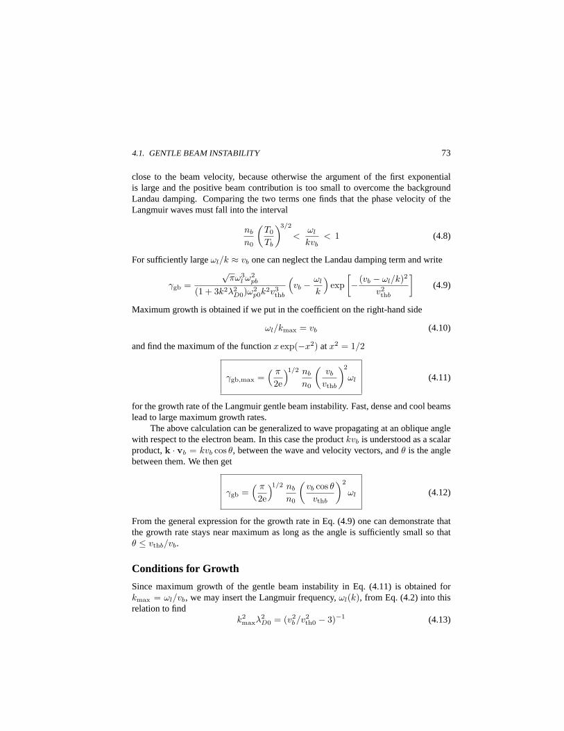
4.1. GENTLE BEAM INSTABILITY 73
close to the beam velocity, because otherwise the argument of the first exponentialis large and the positive beam contribution is too small to overcome the backgroundLandau damping. Comparing the two terms one finds that the phase velocity of theLangmuir waves must fall into the interval
nb
n0
(T0
Tb
)3/2
<ωl
kvb< 1 (4.8)
For sufficiently largeωl/k ≈ vb one can neglect the Landau damping term and write
γgb =
√πω3
l ω2pb
(1 + 3k2λ2D0)ω
2p0k
2v3thb
(vb − ωl
k
)exp
[− (vb − ωl/k)2
v2thb
](4.9)
Maximum growth is obtained if we put in the coefficient on the right-hand side
ωl/kmax = vb (4.10)
and find the maximum of the functionx exp(−x2) atx2 = 1/2
γgb,max =( π
2e
)1/2 nb
n0
(vb
vthb
)2
ωl (4.11)
for the growth rate of the Langmuir gentle beam instability. Fast, dense and cool beamslead to large maximum growth rates.
The above calculation can be generalized to wave propagating at an oblique anglewith respect to the electron beam. In this case the productkvb is understood as a scalarproduct,k · vb = kvb cos θ, between the wave and velocity vectors, andθ is the anglebetween them. We then get
γgb =( π
2e
)1/2 nb
n0
(vb cos θ
vthb
)2
ωl (4.12)
From the general expression for the growth rate in Eq. (4.9) one can demonstrate thatthe growth rate stays near maximum as long as the angle is sufficiently small so thatθ ≤ vthb/vb.
Conditions for Growth
Since maximum growth of the gentle beam instability in Eq. (4.11) is obtained forkmax = ωl/vb, we may insert the Langmuir frequency,ωl(k), from Eq. (4.2) into thisrelation to find
k2maxλ
2D0 = (v2
b/v2th0 − 3)−1 (4.13)
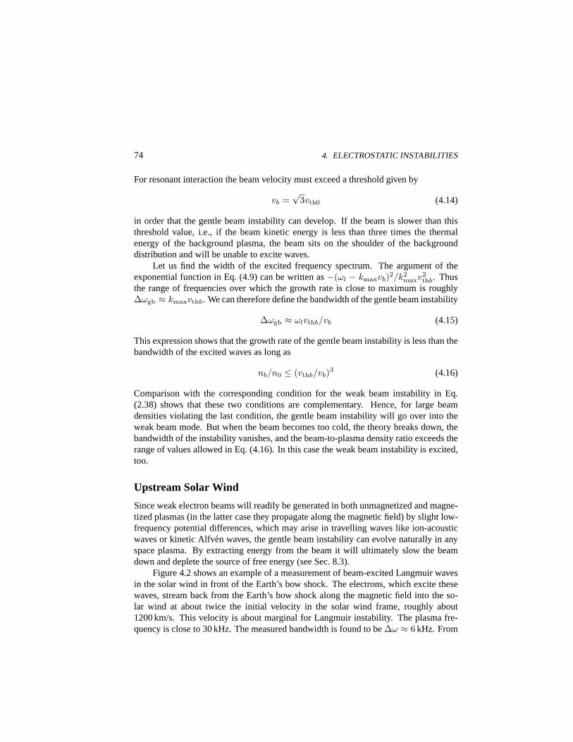
74 4. ELECTROSTATIC INSTABILITIES
For resonant interaction the beam velocity must exceed a threshold given by
vb =√
3vth0 (4.14)
in order that the gentle beam instability can develop. If the beam is slower than thisthreshold value, i.e., if the beam kinetic energy is less than three times the thermalenergy of the background plasma, the beam sits on the shoulder of the backgrounddistribution and will be unable to excite waves.
Let us find the width of the excited frequency spectrum. The argument of theexponential function in Eq. (4.9) can be written as−(ωl − kmaxvb)2/k2
maxv2thb. Thus
the range of frequencies over which the growth rate is close to maximum is roughly∆ωgb ≈ kmaxvthb. We can therefore define the bandwidth of the gentle beam instability
∆ωgb ≈ ωlvthb/vb (4.15)
This expression shows that the growth rate of the gentle beam instability is less than thebandwidth of the excited waves as long as
nb/n0 ≤ (vthb/vb)3 (4.16)
Comparison with the corresponding condition for the weak beam instability in Eq.(2.38) shows that these two conditions are complementary. Hence, for large beamdensities violating the last condition, the gentle beam instability will go over into theweak beam mode. But when the beam becomes too cold, the theory breaks down, thebandwidth of the instability vanishes, and the beam-to-plasma density ratio exceeds therange of values allowed in Eq. (4.16). In this case the weak beam instability is excited,too.
Upstream Solar Wind
Since weak electron beams will readily be generated in both unmagnetized and magne-tized plasmas (in the latter case they propagate along the magnetic field) by slight low-frequency potential differences, which may arise in travelling waves like ion-acousticwaves or kinetic Alfven waves, the gentle beam instability can evolve naturally in anyspace plasma. By extracting energy from the beam it will ultimately slow the beamdown and deplete the source of free energy (see Sec. 8.3).
Figure 4.2 shows an example of a measurement of beam-excited Langmuir wavesin the solar wind in front of the Earth’s bow shock. The electrons, which excite thesewaves, stream back from the Earth’s bow shock along the magnetic field into the so-lar wind at about twice the initial velocity in the solar wind frame, roughly about1200 km/s. This velocity is about marginal for Langmuir instability. The plasma fre-quency is close to 30 kHz. The measured bandwidth is found to be∆ω ≈ 6 kHz. From
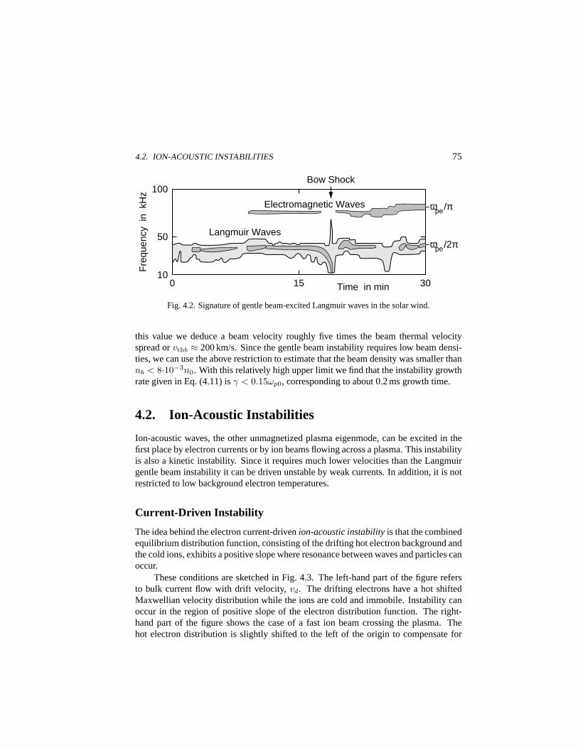
4.2. ION-ACOUSTIC INSTABILITIES 75
100
10
50 ωpe/2π
ωpe/π
Time in min 0 30 15
Fre
quen
cy i
n k
Hz
Bow Shock
Electromagnetic Waves
Langmuir Waves
Fig. 4.2. Signature of gentle beam-excited Langmuir waves in the solar wind.
this value we deduce a beam velocity roughly five times the beam thermal velocityspread orvthb ≈ 200 km/s. Since the gentle beam instability requires low beam densi-ties, we can use the above restriction to estimate that the beam density was smaller thannb < 8·10−3n0. With this relatively high upper limit we find that the instability growthrate given in Eq. (4.11) isγ < 0.15ωp0, corresponding to about 0.2 ms growth time.
4.2. Ion-Acoustic Instabilities
Ion-acoustic waves, the other unmagnetized plasma eigenmode, can be excited in thefirst place by electron currents or by ion beams flowing across a plasma. This instabilityis also a kinetic instability. Since it requires much lower velocities than the Langmuirgentle beam instability it can be driven unstable by weak currents. In addition, it is notrestricted to low background electron temperatures.
Current-Driven Instability
The idea behind the electron current-drivenion-acoustic instabilityis that the combinedequilibrium distribution function, consisting of the drifting hot electron background andthe cold ions, exhibits a positive slope where resonance between waves and particles canoccur.
These conditions are sketched in Fig. 4.3. The left-hand part of the figure refersto bulk current flow with drift velocity,vd. The drifting electrons have a hot shiftedMaxwellian velocity distribution while the ions are cold and immobile. Instability canoccur in the region of positive slope of the electron distribution function. The right-hand part of the figure shows the case of a fast ion beam crossing the plasma. Thehot electron distribution is slightly shifted to the left of the origin to compensate for
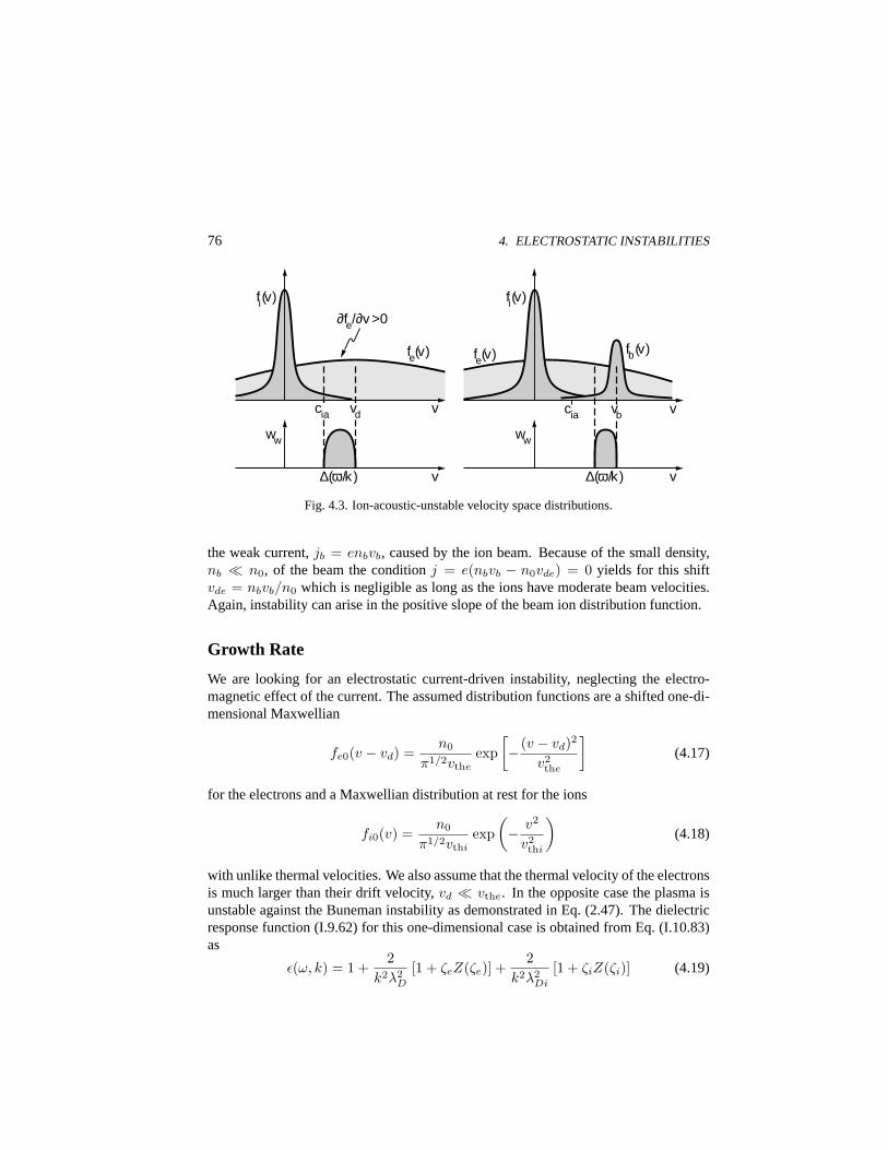
76 4. ELECTROSTATIC INSTABILITIES
cia
fb(v)
vb v cia vd v
fi(v)
v ∆(ω/k )
ww
v ∆(ω/k )
ww
fe(v) fe(v)
fi(v)
∂fe/∂v >0
Fig. 4.3. Ion-acoustic-unstable velocity space distributions.
the weak current,jb = enbvb, caused by the ion beam. Because of the small density,nb ¿ n0, of the beam the conditionj = e(nbvb − n0vde) = 0 yields for this shiftvde = nbvb/n0 which is negligible as long as the ions have moderate beam velocities.Again, instability can arise in the positive slope of the beam ion distribution function.
Growth Rate
We are looking for an electrostatic current-driven instability, neglecting the electro-magnetic effect of the current. The assumed distribution functions are a shifted one-di-mensional Maxwellian
fe0(v − vd) =n0
π1/2vtheexp
[− (v − vd)2
v2the
](4.17)
for the electrons and a Maxwellian distribution at rest for the ions
fi0(v) =n0
π1/2vthiexp
(− v2
v2thi
)(4.18)
with unlike thermal velocities. We also assume that the thermal velocity of the electronsis much larger than their drift velocity,vd ¿ vthe. In the opposite case the plasma isunstable against the Buneman instability as demonstrated in Eq. (2.47). The dielectricresponse function (I.9.62) for this one-dimensional case is obtained from Eq. (I.10.83)as
ε(ω, k) = 1 +2
k2λ2D
[1 + ζeZ(ζe)] +2
k2λ2Di
[1 + ζiZ(ζi)] (4.19)
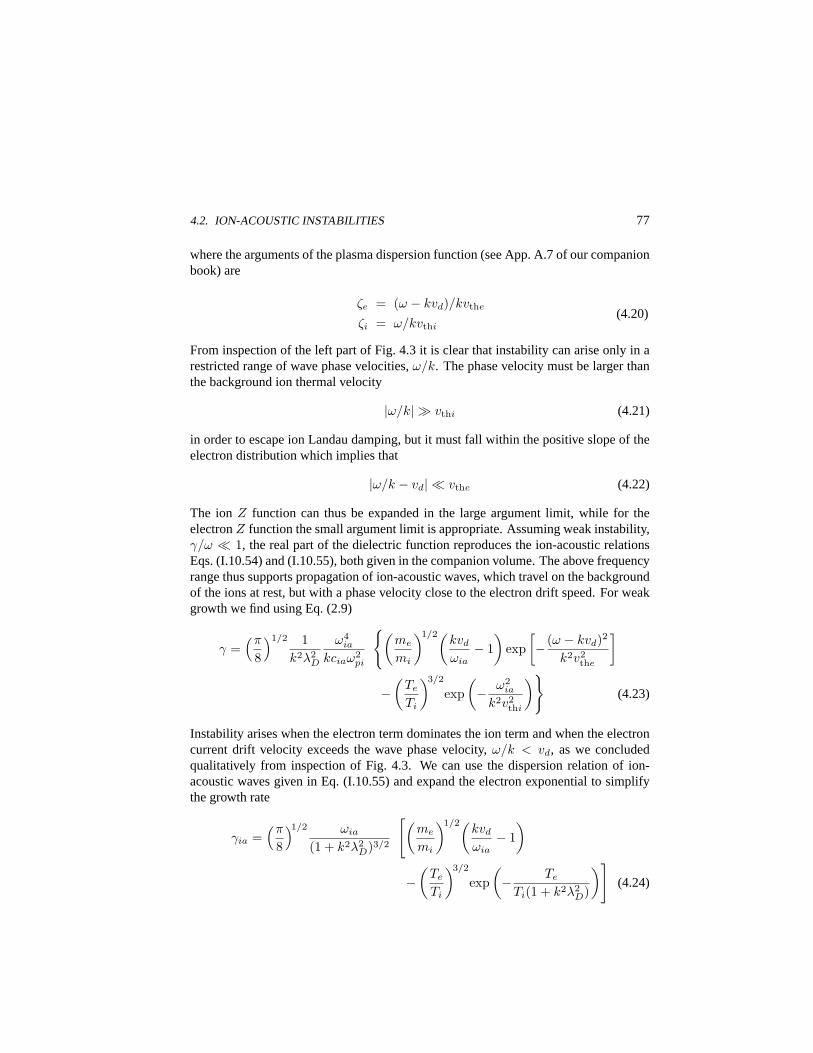
4.2. ION-ACOUSTIC INSTABILITIES 77
where the arguments of the plasma dispersion function (see App. A.7 of our companionbook) are
ζe = (ω − kvd)/kvthe
ζi = ω/kvthi(4.20)
From inspection of the left part of Fig. 4.3 it is clear that instability can arise only in arestricted range of wave phase velocities,ω/k. The phase velocity must be larger thanthe background ion thermal velocity
|ω/k| À vthi (4.21)
in order to escape ion Landau damping, but it must fall within the positive slope of theelectron distribution which implies that
|ω/k − vd| ¿ vthe (4.22)
The ionZ function can thus be expanded in the large argument limit, while for theelectronZ function the small argument limit is appropriate. Assuming weak instability,γ/ω ¿ 1, the real part of the dielectric function reproduces the ion-acoustic relationsEqs. (I.10.54) and (I.10.55), both given in the companion volume. The above frequencyrange thus supports propagation of ion-acoustic waves, which travel on the backgroundof the ions at rest, but with a phase velocity close to the electron drift speed. For weakgrowth we find using Eq. (2.9)
γ =(π
8
)1/2 1k2λ2
D
ω4ia
kciaω2pi
(me
mi
)1/2(kvd
ωia− 1
)exp
[− (ω − kvd)2
k2v2the
]
−(
Te
Ti
)3/2
exp(− ω2
ia
k2v2thi
)(4.23)
Instability arises when the electron term dominates the ion term and when the electroncurrent drift velocity exceeds the wave phase velocity,ω/k < vd, as we concludedqualitatively from inspection of Fig. 4.3. We can use the dispersion relation of ion-acoustic waves given in Eq. (I.10.55) and expand the electron exponential to simplifythe growth rate
γia =(π
8
)1/2 ωia
(1 + k2λ2D)3/2
[(me
mi
)1/2(kvd
ωia− 1
)
−(
Te
Ti
)3/2
exp(− Te
Ti(1 + k2λ2D)
)](4.24)
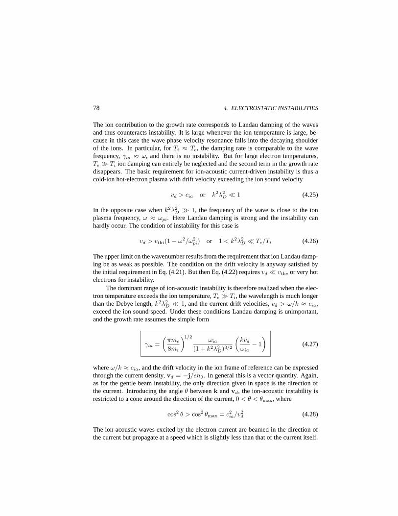
78 4. ELECTROSTATIC INSTABILITIES
The ion contribution to the growth rate corresponds to Landau damping of the wavesand thus counteracts instability. It is large whenever the ion temperature is large, be-cause in this case the wave phase velocity resonance falls into the decaying shoulderof the ions. In particular, forTi ≈ Te, the damping rate is comparable to the wavefrequency,γia ≈ ω, and there is no instability. But for large electron temperatures,Te À Ti ion damping can entirely be neglected and the second term in the growth ratedisappears. The basic requirement for ion-acoustic current-driven instability is thus acold-ion hot-electron plasma with drift velocity exceeding the ion sound velocity
vd > cia or k2λ2D ¿ 1 (4.25)
In the opposite case whenk2λ2D À 1, the frequency of the wave is close to the ion
plasma frequency,ω ≈ ωpi. Here Landau damping is strong and the instability canhardly occur. The condition of instability for this case is
vd > vthi(1− ω2/ω2pi) or 1 < k2λ2
D ¿ Te/Ti (4.26)
The upper limit on the wavenumber results from the requirement that ion Landau damp-ing be as weak as possible. The condition on the drift velocity is anyway satisfied bythe initial requirement in Eq. (4.21). But then Eq. (4.22) requiresvd ¿ vthe or very hotelectrons for instability.
The dominant range of ion-acoustic instability is therefore realized when the elec-tron temperature exceeds the ion temperature,Te À Ti, the wavelength is much longerthan the Debye length,k2λ2
D ¿ 1, and the current drift velocities,vd > ω/k ≈ cia,exceed the ion sound speed. Under these conditions Landau damping is unimportant,and the growth rate assumes the simple form
γia =(
πme
8mi
)1/2ωia
(1 + k2λ2D)3/2
(kvd
ωia− 1
)(4.27)
whereω/k ≈ cia, and the drift velocity in the ion frame of reference can be expressedthrough the current density,vd = −j/en0. In general this is a vector quantity. Again,as for the gentle beam instability, the only direction given in space is the direction ofthe current. Introducing the angleθ betweenk andvd, the ion-acoustic instability isrestricted to a cone around the direction of the current,0 < θ < θmax, where
cos2 θ > cos2 θmax = c2ia/v2
d (4.28)
The ion-acoustic waves excited by the electron current are beamed in the direction ofthe current but propagate at a speed which is slightly less than that of the current itself.
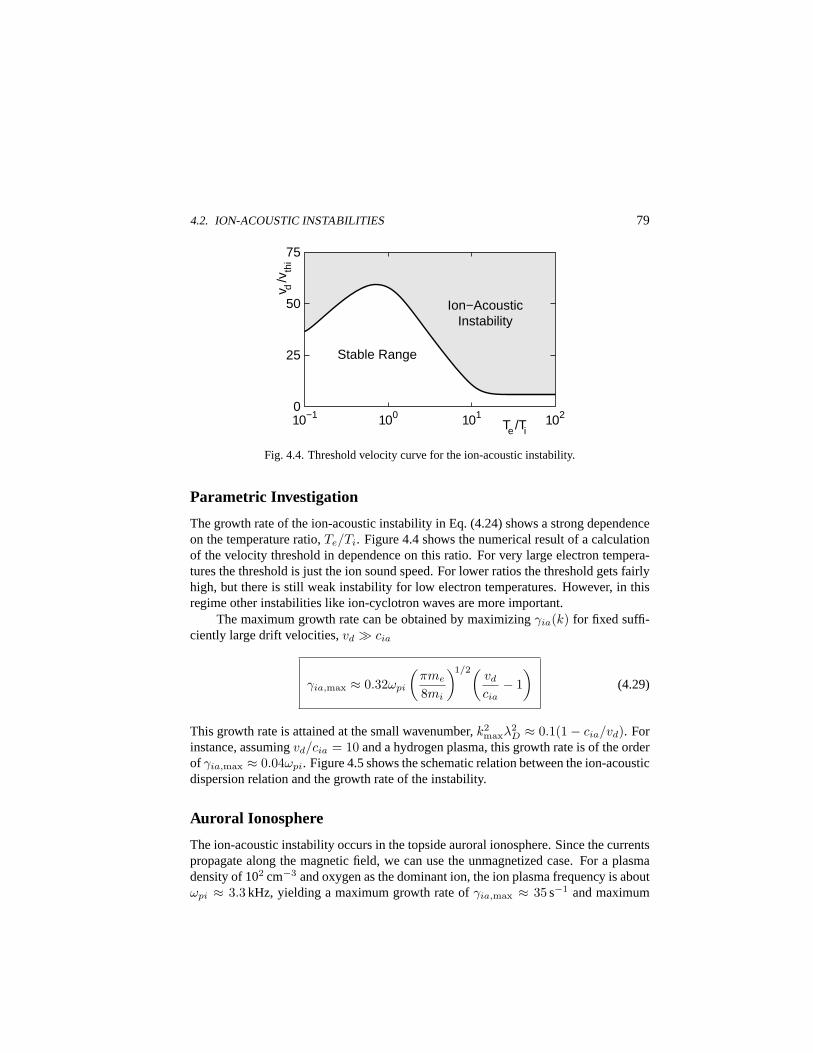
4.2. ION-ACOUSTIC INSTABILITIES 79
0
25
50
75
10−1 100 101 102
Ion−Acoustic Instability
Stable Range
Te /Ti
v d/v
thi
Fig. 4.4. Threshold velocity curve for the ion-acoustic instability.
Parametric Investigation
The growth rate of the ion-acoustic instability in Eq. (4.24) shows a strong dependenceon the temperature ratio,Te/Ti. Figure 4.4 shows the numerical result of a calculationof the velocity threshold in dependence on this ratio. For very large electron tempera-tures the threshold is just the ion sound speed. For lower ratios the threshold gets fairlyhigh, but there is still weak instability for low electron temperatures. However, in thisregime other instabilities like ion-cyclotron waves are more important.
The maximum growth rate can be obtained by maximizingγia(k) for fixed suffi-ciently large drift velocities,vd À cia
γia,max ≈ 0.32ωpi
(πme
8mi
)1/2(vd
cia− 1
)(4.29)
This growth rate is attained at the small wavenumber,k2maxλ
2D ≈ 0.1(1− cia/vd). For
instance, assumingvd/cia = 10 and a hydrogen plasma, this growth rate is of the orderof γia,max ≈ 0.04ωpi. Figure 4.5 shows the schematic relation between the ion-acousticdispersion relation and the growth rate of the instability.
Auroral Ionosphere
The ion-acoustic instability occurs in the topside auroral ionosphere. Since the currentspropagate along the magnetic field, we can use the unmagnetized case. For a plasmadensity of 102 cm−3 and oxygen as the dominant ion, the ion plasma frequency is aboutωpi ≈ 3.3 kHz, yielding a maximum growth rate ofγia,max ≈ 35 s−1 and maximum
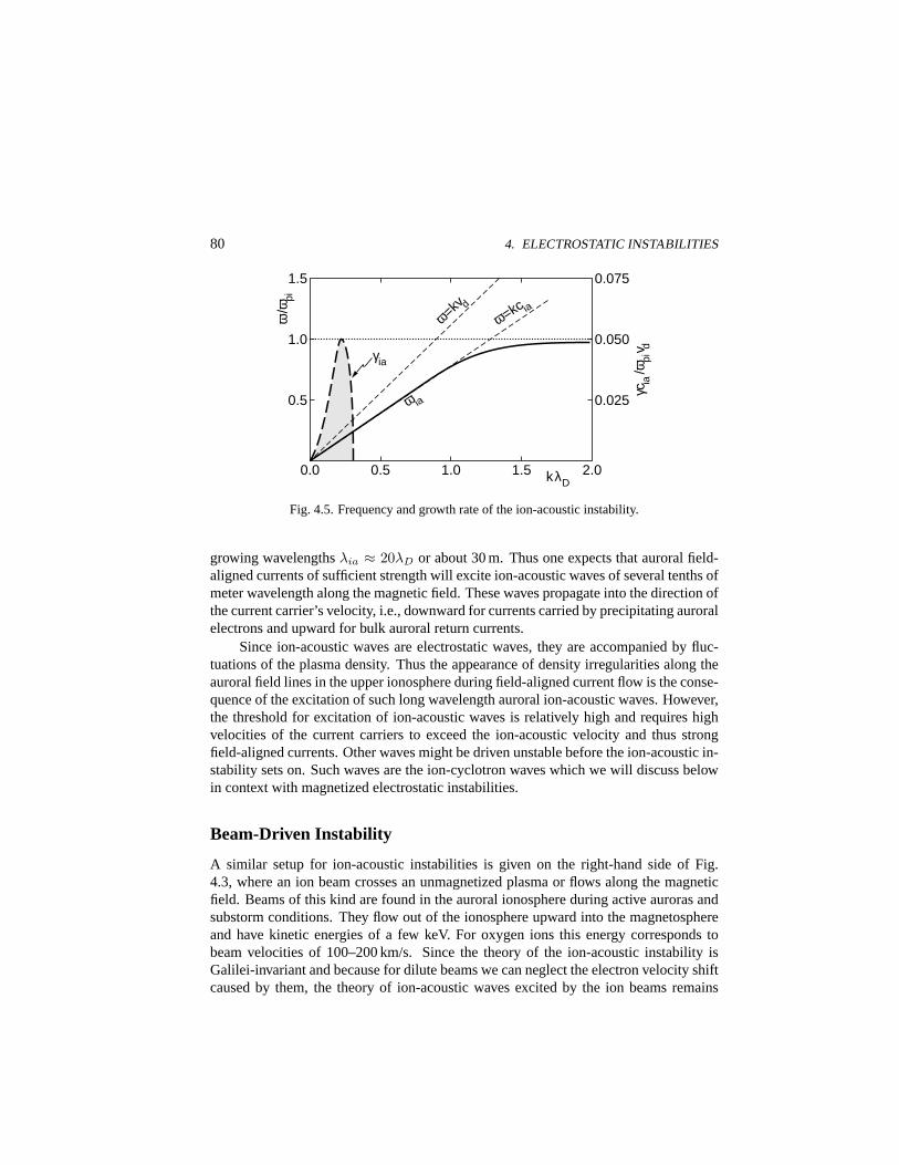
80 4. ELECTROSTATIC INSTABILITIES
1.0
ω=kc iaω=kv d
ω ia
kλD
ω/ω
pi
γcia
/ωpi
v d
0.0
γia
2.0
1.0
1.5
0.5
0.5 1.5
0.050
0.075
0.025
Fig. 4.5. Frequency and growth rate of the ion-acoustic instability.
growing wavelengthsλia ≈ 20λD or about 30 m. Thus one expects that auroral field-aligned currents of sufficient strength will excite ion-acoustic waves of several tenths ofmeter wavelength along the magnetic field. These waves propagate into the direction ofthe current carrier’s velocity, i.e., downward for currents carried by precipitating auroralelectrons and upward for bulk auroral return currents.
Since ion-acoustic waves are electrostatic waves, they are accompanied by fluc-tuations of the plasma density. Thus the appearance of density irregularities along theauroral field lines in the upper ionosphere during field-aligned current flow is the conse-quence of the excitation of such long wavelength auroral ion-acoustic waves. However,the threshold for excitation of ion-acoustic waves is relatively high and requires highvelocities of the current carriers to exceed the ion-acoustic velocity and thus strongfield-aligned currents. Other waves might be driven unstable before the ion-acoustic in-stability sets on. Such waves are the ion-cyclotron waves which we will discuss belowin context with magnetized electrostatic instabilities.
Beam-Driven Instability
A similar setup for ion-acoustic instabilities is given on the right-hand side of Fig.4.3, where an ion beam crosses an unmagnetized plasma or flows along the magneticfield. Beams of this kind are found in the auroral ionosphere during active auroras andsubstorm conditions. They flow out of the ionosphere upward into the magnetosphereand have kinetic energies of a few keV. For oxygen ions this energy corresponds tobeam velocities of 100–200 km/s. Since the theory of the ion-acoustic instability isGalilei-invariant and because for dilute beams we can neglect the electron velocity shiftcaused by them, the theory of ion-acoustic waves excited by the ion beams remains

4.2. ION-ACOUSTIC INSTABILITIES 81
unchanged. The beam will excite ion-acoustic waves propagating close to the beamvelocity if far enough away from the thermal electron distribution for not being Landaudamped. The condition for instability is
ω/k À vthe (4.30)
and the growth rate can be written as
γiab =(π
8
)1/2 ω4
ω2pi|k|3ciaλ2
D
nib
n0
(Te
Tib
)1/2
(kvb
ω− 1
)exp
[− (ω − kvb)2
k2v2thib
]−
(me
mi
)1/2
exp(− ω2
k2v2the
)(4.31)
where we neglected the contribution of the background ions, and the total density isn0 = ne0 = ni0 + nib. The condition for beam ion-acoustic instability is the sameas for current instability with replacement of the current drift speed by the ion beamvelocity,vib > cia. Compared to the electron current-driven instability this growth rateis smaller by the ratio of beam to plasma densities. Thus the ion beam driven mode is aweaker instability than the electron current ion-acoustic instability.
Heat Flux-Driven Instability
Ion-acoustic waves can also be destabilized by heat currents. These currents play a rolesimilar to real electric currents in a plasma. But they depend on the presence of heatflows and thus on the presence of temperature gradients in a plasma. Such temperaturegradients are familiar from observations in the solar wind, at the magnetopause and inthe various boundary layers of the magnetosphere. One may therefore expect that heatflux-driven ion-acoustic modes will exist in these regions.
In most cases the heat flux is carried by electrons, since they move faster alongthe magnetic field. The mechanism of the instability is exactly the same as that for theelectron current-driven ion-acoustic instability. The only difference is that the electrondrift speed is now calculated from the parallel heat flux,q‖, under the condition that theelectric current vanishes,j‖ = 0. The two equations for the parallel heat flux and cur-rent in a zero-order parallel electric field,E0‖, and parallel temperature gradient∇‖Te,are
qe‖ = ηe‖E0‖ − κe‖∇‖Te
je‖ = σe‖E0‖ + ζe‖∇‖Te = 0(4.32)
Heat fluxes can evolve only in the presence of non-vanishing transport coefficients(see App. B.2 in our companion book). We therefore allow for non-ideal conditions

82 4. ELECTROSTATIC INSTABILITIES
and finite electric and thermal conductivities,σe‖, κe‖, and thermoelectric conductiv-ities, ηe‖, ζe‖. From the definition of the transport coefficients one knows thatζe‖ ≈0.7σe‖/e. The vanishing current equation yields for the electric field
E0‖ ≈ −0.7∇‖Te/e (4.33)
This electric field enters the heat flux equation so that
qe‖ ≈ −(κe‖ − 0.7ηe‖/e)∇‖Te (4.34)
from where it is seen that it is the temperature gradient which gives rise to the heat fluxor, vice versa, it is the heat flux which causes the parallel electric field. This electricfield accelerates the electrons until a stationary state is reached between the accelerationand collisional retardation due to the non-zero electron-ion collision frequency,νei 6= 0.Equating the two forces
eE0‖ = meνeivd (4.35)
the drift velocity enforced by the heat flux and being used in the growth rate of theion-acoustic instability in Eq. (4.27) is given by
vd ≈ 0.7∇‖Te/meνei > cia (4.36)
This is the condition for ion acoustic instability.
Solar Wind
In a nearly collisionless plasma like the solar wind the collision frequency is smalland the instability threshold is easily exceeded, even for weak temperature gradients.There is no unambiguous experimental confirmation of a heat flux-driven instability inthe solar wind from observations of ion-acoustic waves, but heat fluxes are connectedwith most deviations of the parallel electron equilibrium distribution from Maxwelliansymmetry. Such non-symmetric shapes are a general feature of solar wind electrondistributions and can be the cause of heat flux-excited ion-acoustic waves.
4.3. Electron-Acoustic Instability
To excite electron-acoustic waves a drifting hot electron component is needed in addi-tion to the cold background electrons. The ions are assumed to neutralize the charge.Moreover, zero current flow is assumed for the electrons,ncvdc + nhvdh = 0. Forvanishing drifts and low cold electron temperatures three weakly damped modes canexist. These are Langmuir waves, ion-acoustic waves and electron-acoustic waves. Thefrequency of the latter is close to the cold electron plasma frequency,ωea ≈ ωpc. When
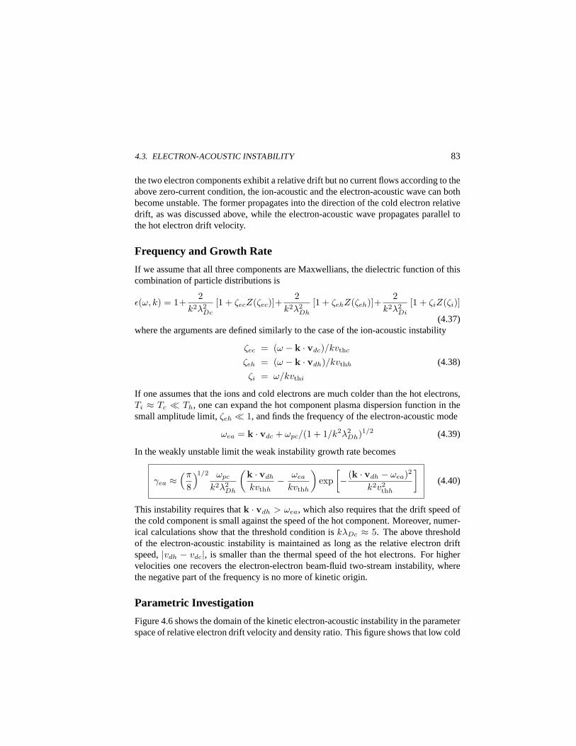
4.3. ELECTRON-ACOUSTIC INSTABILITY 83
the two electron components exhibit a relative drift but no current flows according to theabove zero-current condition, the ion-acoustic and the electron-acoustic wave can bothbecome unstable. The former propagates into the direction of the cold electron relativedrift, as was discussed above, while the electron-acoustic wave propagates parallel tothe hot electron drift velocity.
Frequency and Growth Rate
If we assume that all three components are Maxwellians, the dielectric function of thiscombination of particle distributions is
ε(ω, k) = 1+2
k2λ2Dc
[1 + ζecZ(ζec)]+2
k2λ2Dh
[1 + ζehZ(ζeh)]+2
k2λ2Di
[1 + ζiZ(ζi)]
(4.37)where the arguments are defined similarly to the case of the ion-acoustic instability
ζec = (ω − k · vdc)/kvthc
ζeh = (ω − k · vdh)/kvthh (4.38)
ζi = ω/kvthi
If one assumes that the ions and cold electrons are much colder than the hot electrons,Ti ≈ Tc ¿ Th, one can expand the hot component plasma dispersion function in thesmall amplitude limit,ζeh ¿ 1, and finds the frequency of the electron-acoustic mode
ωea = k · vdc + ωpc/(1 + 1/k2λ2Dh)1/2 (4.39)
In the weakly unstable limit the weak instability growth rate becomes
γea ≈(π
8
)1/2 ωpc
k2λ2Dh
(k · vdh
kvthh− ωea
kvthh
)exp
[− (k · vdh − ωea)2
k2v2thh
](4.40)
This instability requires thatk · vdh > ωea, which also requires that the drift speed ofthe cold component is small against the speed of the hot component. Moreover, numer-ical calculations show that the threshold condition iskλDc ≈ 5. The above thresholdof the electron-acoustic instability is maintained as long as the relative electron driftspeed,|vdh − vdc|, is smaller than the thermal speed of the hot electrons. For highervelocities one recovers the electron-electron beam-fluid two-stream instability, wherethe negative part of the frequency is no more of kinetic origin.
Parametric Investigation
Figure 4.6 shows the domain of the kinetic electron-acoustic instability in the parameterspace of relative electron drift velocity and density ratio. This figure shows that low cold
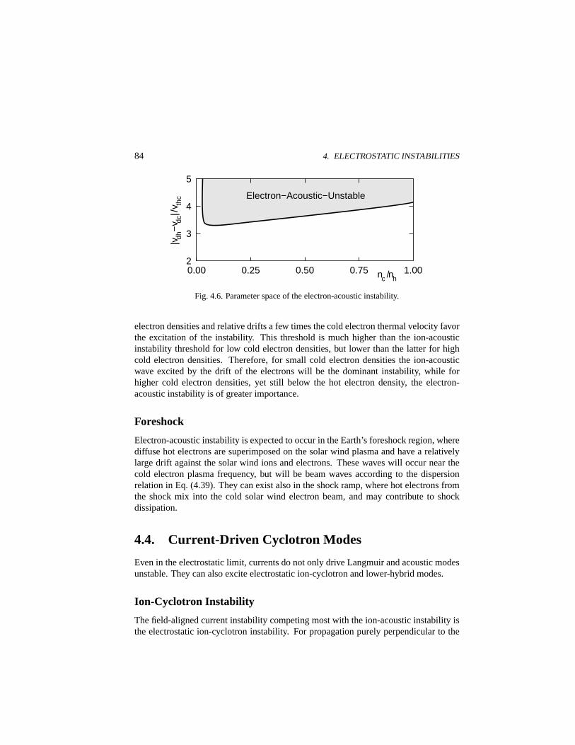
84 4. ELECTROSTATIC INSTABILITIES
Electron−Acoustic−Unstable
0.00 0.50 1.00 nc /nh
|v dh−
v dc|/
v thc
2
5
3
4
0.25 0.75
Fig. 4.6. Parameter space of the electron-acoustic instability.
electron densities and relative drifts a few times the cold electron thermal velocity favorthe excitation of the instability. This threshold is much higher than the ion-acousticinstability threshold for low cold electron densities, but lower than the latter for highcold electron densities. Therefore, for small cold electron densities the ion-acousticwave excited by the drift of the electrons will be the dominant instability, while forhigher cold electron densities, yet still below the hot electron density, the electron-acoustic instability is of greater importance.
Foreshock
Electron-acoustic instability is expected to occur in the Earth’s foreshock region, wherediffuse hot electrons are superimposed on the solar wind plasma and have a relativelylarge drift against the solar wind ions and electrons. These waves will occur near thecold electron plasma frequency, but will be beam waves according to the dispersionrelation in Eq. (4.39). They can exist also in the shock ramp, where hot electrons fromthe shock mix into the cold solar wind electron beam, and may contribute to shockdissipation.
4.4. Current-Driven Cyclotron Modes
Even in the electrostatic limit, currents do not only drive Langmuir and acoustic modesunstable. They can also excite electrostatic ion-cyclotron and lower-hybrid modes.
Ion-Cyclotron Instability
The field-aligned current instability competing most with the ion-acoustic instability isthe electrostatic ion-cyclotron instability. For propagation purely perpendicular to the
4.4. CURRENT-DRIVEN CYCLOTRON MODES 85
magnetic field its dispersion relation is that of Eq. (I.10.133) and the wave is an ionBernstein mode. To find an instability we must allow parallel wave propagation. In thiscase the dispersion relation is a version of Eq. (I.10.104), modified due to the presenceof the field-aligned current. Assuming that this current is carried exclusively by theelectrons, its dielectric function becomes
ε(ω,k) = 1−∑
s
∞∑
l=−∞
ω2psΛl(ηs)k2v2
ths
[Z ′(ζs)− 2lωgs
k‖vthsZ(ζs)
]= 0 (4.41)
We assume isotropic conditions for both kinds of particles, electrons and ions. The ar-guments of the plasma dispersion functions are
ζi = (ω − lωgi)/k‖vthi
ζe = (ω + lωge − k‖vd)/k‖vthe(4.42)
The above dispersion relation allows instability at every ion-cyclotron harmonic fre-quency,ω = lωgi. For purely parallel propagation andTe À Ti it also containsion-acoustic waves, since this case corresponds to the field-free case. Hence, to coverion-cyclotron waves we consider the wavenumber rangek‖ ¿ k⊥, and temperatureratiosTe ≈ Ti. We may expect that the strongest instability will occur for the low-est harmonic,l = 1, because it requires the smallest amount of energy to increase itsamplitude. The ion-cyclotron wave solution
ω ≈ ωgi
[1 +
Λ1(ηi)1 + Ti/Ti −G
](4.43)
whereG = Λ1 + (1 − Λ0)/ηi, is obtained under the conditions thatηe ¿ 1 and, asfor the ion-acoustic instability,ζe ¿ 1, while the ion plasma dispersion function isexpanded in the large argument limit.
SinceG < 1, Λ1 < 1, the correction term on the cyclotron frequency is usuallysmaller than 0.5, so that the frequency of the ion-cyclotron wave is close toωgi, butshifts away fromωgi for decreasingTe/Ti. On the other hand, whenTe À Ti andηi ¿ 1, the termG → 1, and the correction increases. In the limitηi → 0 thefrequency becomes
ω ≈ ωgi(1 + k2⊥c2
ia/2ω2gi) = ωgi(1 + ∆) (4.44)
valid in the long wavelength limit and applicable to perpendicular propagation.For oblique propagation the expression for the growth rate is complicated. It is
more interesting to determine the marginally unstable current drift velocity for the ioncyclotron wave above which the instability sets in. The procedure is to put the growthrateγ = 0 in the dielectric response, setting its real partεr(ω, k‖, k⊥) = 0, and solving
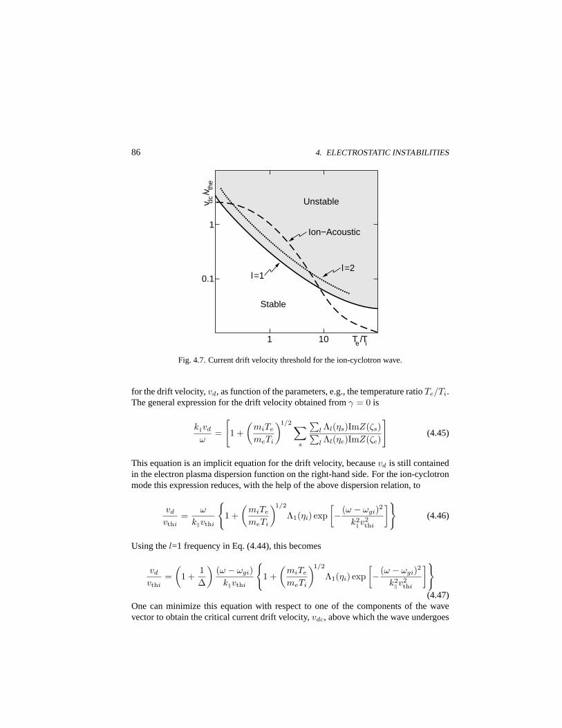
86 4. ELECTROSTATIC INSTABILITIES
Unstable
Stable
Ion−Acoustic
l=2 l=1 0.1
1
1 10 Te/Ti
v dc/v th
e
Fig. 4.7. Current drift velocity threshold for the ion-cyclotron wave.
for the drift velocity,vd, as function of the parameters, e.g., the temperature ratioTe/Ti.The general expression for the drift velocity obtained fromγ = 0 is
k‖vd
ω=
[1 +
(miTe
meTi
)1/2 ∑s
∑l Λl(ηs)ImZ(ζs)∑l Λl(ηe)ImZ(ζe)
](4.45)
This equation is an implicit equation for the drift velocity, becausevd is still containedin the electron plasma dispersion function on the right-hand side. For the ion-cyclotronmode this expression reduces, with the help of the above dispersion relation, to
vd
vthi=
ω
k‖vthi
1 +
(miTe
meTi
)1/2
Λ1(ηi) exp[− (ω − ωgi)2
k2‖v
2thi
](4.46)
Using thel=1 frequency in Eq. (4.44), this becomes
vd
vthi=
(1 +
1∆
)(ω − ωgi)
k‖vthi
1 +
(miTe
meTi
)1/2
Λ1(ηi) exp[− (ω − ωgi)2
k2‖v
2thi
]
(4.47)One can minimize this equation with respect to one of the components of the wavevector to obtain the critical current drift velocity,vdc, above which the wave undergoes
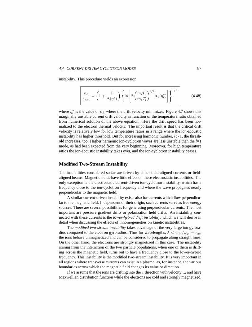
4.4. CURRENT-DRIVEN CYCLOTRON MODES 87
instability. This procedure yields an expression
vdc
vthi=
(1 +
1∆(η∗i )
) ln
[2
(miTe
meTi
)1/2
Λ1(η∗i )
]1/2
(4.48)
whereη∗i is the value ofk⊥ where the drift velocity minimizes. Figure 4.7 shows thismarginally unstable current drift velocity as function of the temperature ratio obtainedfrom numerical solution of the above equation. Here the drift speed has been nor-malized to the electron thermal velocity. The important result is that the critical driftvelocity is relatively low for low temperature ratios in a range where the ion-acousticinstability has higher threshold. But for increasing harmonic number,l>1, the thresh-old increases, too. Higher harmonic ion-cyclotron waves are less unstable than thel=1mode, as had been expected from the very beginning. Moreover, for high temperatureratios the ion-acoustic instability takes over, and the ion-cyclotron instability ceases.
Modified Two-Stream Instability
The instabilities considered so far are driven by either field-aligned currents or field-aligned beams. Magnetic fields have little effect on these electrostatic instabilities. Theonly exception is the electrostatic current-driven ion-cyclotron instability, which has afrequency close to the ion-cyclotron frequency and where the wave propagates nearlyperpendicular to the magnetic field.
A similar current-driven instability exists also for currents which flow perpendicu-lar to the magnetic field. Independent of their origin, such currents serve as free energysources. There are several possibilities for generating perpendicular currents. The mostimportant are pressure gradient drifts or polarization field drifts. An instability con-nected with these currents is thelower-hybrid drift instability, which we will derive indetail when discussing the effects of inhomogeneities on kinetic instabilities.
Themodified two-stream instabilitytakes advantage of the very large ion gyrora-dius compared to the electron gyroradius. Thus for wavelengths,λ < vthi/ωgi = rgi,the ions behave unmagnetized and can be considered to propagate along straight lines.On the other hand, the electrons are strongly magnetized in this case. The instabilityarising from the interaction of the two particle populations, when one of them is drift-ing across the magnetic field, turns out to have a frequency close to the lower-hybridfrequency. This instability is the modified two-stream instability. It is very important inall regions where transverse currents can exist in a plasma, as, for instance, the variousboundaries across which the magnetic field changes its value or direction.
If we assume that the ions are drifting into thex direction with velocityvd and haveMaxwellian distribution function while the electrons are cold and strongly magnetized,
88 4. ELECTROSTATIC INSTABILITIES
the wave obeys the dispersion relation
ε(ω, k‖, k⊥) = 1 +ω2
pe
ω2ge
− k2‖
k2
ω2pe
ω2+
2ω2pi
k2⊥v2
thi
[1 + ζiZ(ζi)] (4.49)
where the ion argument is given byζi = (ω−k⊥vd)/k⊥vthi. This argument is assumedto be large enough,ζi À 1, for the large argument expansion of the plasma dispersionto be applicable so that the dispersion relation becomes
1− ω2lh
(ω − k⊥vd)2− mik
2‖
mek2
ω2lh
ω2= 0 (4.50)
an expression very similar to the Buneman dispersion relation. The frequency,ωlh =ωpi/(1+ω2
pe/ω2ge)
1/2, appearing in the numerators of the above equation, is the lower-hybrid frequency. The similarity of Eq. (4.50) to the Buneman dispersion relation
1− ω2pi
ω2− ω2
pe
(ω − kv0)2= 0 (4.51)
suggests the following replacements in the equations for the latter
ωpe → ωlh
ω2pi → (mik
2‖/mek
2)ω2lh
(4.52)
By the same reasoning used to derive the threshold condition in Eq. (2.50) for the Bune-man instability we find that the frequency of the modified two-stream instability is
ωmts = k⊥vb
[1 +
(mek
2
mik2‖
)1/3]−1
(4.53)
and as condition on the drift velocity for modified two-stream instability
k2⊥v2
b
ω2lh
<
(mek
2
mik2‖
)1/3[1 +
(mik
2‖
mek2
)1/3]3
(4.54)
As in the case of the Buneman instability, this condition sets a limit on the combinationof wavenumber and drift velocity. Since the right-hand side of this condition dependson the lower-hybrid frequency, which is lower than the electron plasma frequency, themodified two-stream instability is driven unstable by much lower velocities than theBuneman instability.
4.4. CURRENT-DRIVEN CYCLOTRON MODES 89
Since in the discussion of the Buneman instability the densities of the particleswere equal, the maximum growing wavenumber now is found at
max(
k2‖
k2⊥
)=
me
mi¿ 1 (4.55)
Hence, the parallel wavelength of the modified two-stream wave is much longer than theperpendicular wavelength and the wave propagates nearly perpendicular to the magneticfield. Its maximum growth rate
γmts,max = ωlh/2 (4.56)
is obtained atk⊥maxvd ≈ ωlh/2 (4.57)
if the growth rate is maximized with respect tok⊥. This growth rate is nearly thelower-hybrid frequency and thus nearly the wave frequency itself.
The modified two-stream instability is a fairly strong instability which will eas-ily be driven unstable by ion streams propagating perpendicular to the magnetic field.Knowing the drift velocity of these ions or the corresponding current, the wave fre-quency at maximum growth assumes the value
ωmts,max = k⊥maxvd/2 (4.58)
Magnetopause
The modified two-stream instability can be excited at the magnetopause, during timeswhen it is a tangential discontinuity. Assuming a non-zero magnetosheath field of about30–40 nT, the jump in the magnetic field across the magnetopause is of the order of∆B ≈ 60 nT. The width of the magnetopause is of the order of 1000 km or less. Thesevalues suggest a current of4.8 · 10−8 A/m2. For a plasma density ofn ≈ 30 cm−3 thedrift velocity is vd ≈ 10 km/s. The lower-hybrid frequency is of the order of 65 Hz.This corresponds to a maximum perpendicular wavenumber ofk⊥ ≈ 0.082 and a wavegrowth rate of 200 s−1.
Hence, fast growth at the lower-hybrid frequency is expected at the magnetopausewith wavelengths of the order of 70 m, shorter than the ion gyroradius. These wavesaccount for lower-hybrid wave spectra observed during magnetopause crossing and willbe able to dissipate part of the kinetic energy of the magnetopause current. This cur-rent is continuously restored by the interaction of solar wind and geomagnetic field.The energy fed into the modified two-stream lower-hybrid waves originates from thisinteraction and thus from the solar wind kinetic energy.
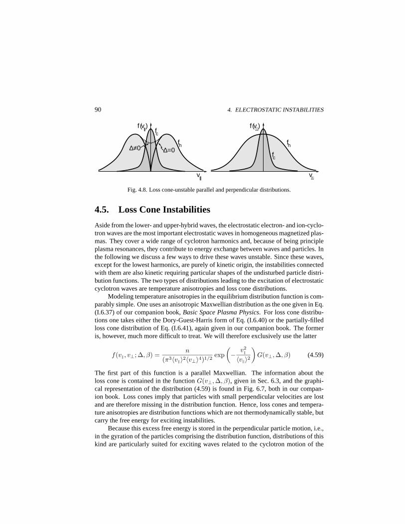
90 4. ELECTROSTATIC INSTABILITIES
∆≠0 ∆=0
v||
fc
fh
f (v||)
fh
fc
v⊥
f (v⊥)
Fig. 4.8. Loss cone-unstable parallel and perpendicular distributions.
4.5. Loss Cone Instabilities
Aside from the lower- and upper-hybrid waves, the electrostatic electron- and ion-cyclo-tron waves are the most important electrostatic waves in homogeneous magnetized plas-mas. They cover a wide range of cyclotron harmonics and, because of being principleplasma resonances, they contribute to energy exchange between waves and particles. Inthe following we discuss a few ways to drive these waves unstable. Since these waves,except for the lowest harmonics, are purely of kinetic origin, the instabilities connectedwith them are also kinetic requiring particular shapes of the undisturbed particle distri-bution functions. The two types of distributions leading to the excitation of electrostaticcyclotron waves are temperature anisotropies and loss cone distributions.
Modeling temperature anisotropies in the equilibrium distribution function is com-parably simple. One uses an anisotropic Maxwellian distribution as the one given in Eq.(I.6.37) of our companion book,Basic Space Plasma Physics. For loss cone distribu-tions one takes either the Dory-Guest-Harris form of Eq. (I.6.40) or the partially-filledloss cone distribution of Eq. (I.6.41), again given in our companion book. The formeris, however, much more difficult to treat. We will therefore exclusively use the latter
f(v‖, v⊥;∆, β) =n
(π3〈v‖〉2〈v⊥〉4)1/2exp
(− v2
‖
〈v‖〉2)
G(v⊥,∆, β) (4.59)
The first part of this function is a parallel Maxwellian. The information about theloss cone is contained in the functionG(v⊥, ∆, β), given in Sec. 6.3, and the graphi-cal representation of the distribution (4.59) is found in Fig. 6.7, both in our compan-ion book. Loss cones imply that particles with small perpendicular velocities are lostand are therefore missing in the distribution function. Hence, loss cones and tempera-ture anisotropies are distribution functions which are not thermodynamically stable, butcarry the free energy for exciting instabilities.
Because this excess free energy is stored in the perpendicular particle motion, i.e.,in the gyration of the particles comprising the distribution function, distributions of thiskind are particularly suited for exciting waves related to the cyclotron motion of the
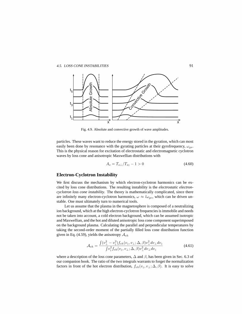
4.5. LOSS CONE INSTABILITIES 91
t1
t3
t5
Conve
ctive
Gro
wth
x x
Abs
olut
e G
row
th
Fig. 4.9. Absolute and convective growth of wave amplitudes.
particles. These waves want to reduce the energy stored in the gyration, which can mosteasily been done by resonance with the gyrating particles at their gyrofrequency,ωgs.This is the physical reason for excitation of electrostatic and electromagnetic cyclotronwaves by loss cone and anisotropic Maxwellian distributions with
As = Ts⊥/Ts‖ − 1 > 0 (4.60)
Electron-Cyclotron Instability
We first discuss the mechanism by which electron-cyclotron harmonics can be ex-cited by loss cone distributions. The resulting instability is theelectrostatic electron-cyclotron loss cone instability. The theory is mathematically complicated, since thereare infinitely many electron-cyclotron harmonics,ω ≈ lωge, which can be driven un-stable. One must ultimately turn to numerical tools.
Let us assume that the plasma in the magnetosphere is composed of a neutralizingion background, which at the high electron-cyclotron frequencies is immobile and needsnot be taken into account, a cold electron background, which can be assumed isotropicand Maxwellian, and the hot and diluted anisotropic loss cone component superimposedon the background plasma. Calculating the parallel and perpendicular temperatures bytaking the second-order moment of the partially filled loss cone distribution functiongiven in Eq. (4.59), yields the anisotropyAeh
Aeh =
∫(v2⊥ − v2
‖)feh(v‖, v⊥;∆, β)v2⊥dv⊥dv‖∫
v2‖feh(v‖, v⊥;∆, β)v2
⊥dv⊥dv‖(4.61)
where a description of the loss cone parameters,∆ andβ, has been given in Sec. 6.3 ofour companion book. The ratio of the two integrals warrants to forget the normalizationfactors in front of the hot electron distribution,feh(v‖, v⊥;∆, β). It is easy to solve
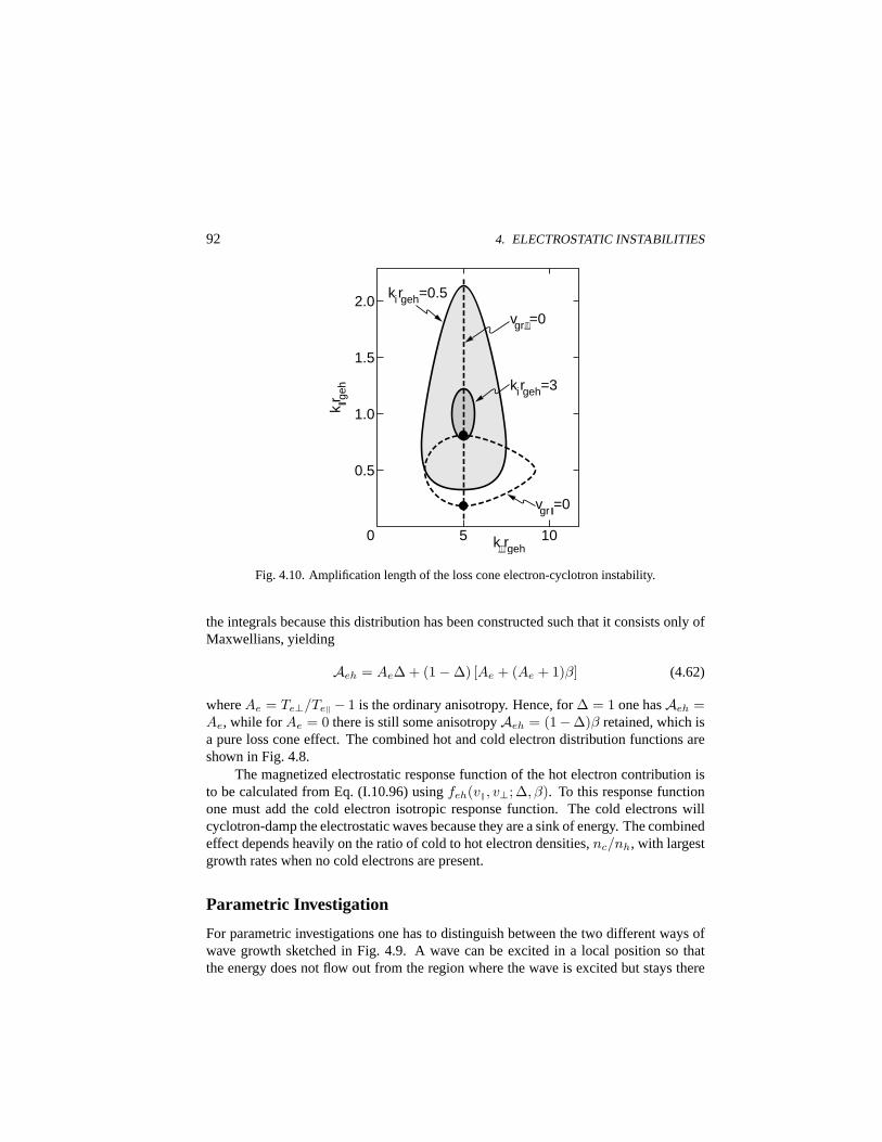
92 4. ELECTROSTATIC INSTABILITIES
0
0.5
1.0
1.5
2.0
5 10 k⊥rgeh
k ||r geh
kirgeh=0.5
vgr⊥=0
vgr ||=0
kirgeh=3
Fig. 4.10. Amplification length of the loss cone electron-cyclotron instability.
the integrals because this distribution has been constructed such that it consists only ofMaxwellians, yielding
Aeh = Ae∆ + (1−∆) [Ae + (Ae + 1)β] (4.62)
whereAe = Te⊥/Te‖ − 1 is the ordinary anisotropy. Hence, for∆ = 1 one hasAeh =Ae, while for Ae = 0 there is still some anisotropyAeh = (1−∆)β retained, which isa pure loss cone effect. The combined hot and cold electron distribution functions areshown in Fig. 4.8.
The magnetized electrostatic response function of the hot electron contribution isto be calculated from Eq. (I.10.96) usingfeh(v‖, v⊥;∆, β). To this response functionone must add the cold electron isotropic response function. The cold electrons willcyclotron-damp the electrostatic waves because they are a sink of energy. The combinedeffect depends heavily on the ratio of cold to hot electron densities,nc/nh, with largestgrowth rates when no cold electrons are present.
Parametric Investigation
For parametric investigations one has to distinguish between the two different ways ofwave growth sketched in Fig. 4.9. A wave can be excited in a local position so thatthe energy does not flow out from the region where the wave is excited but stays there
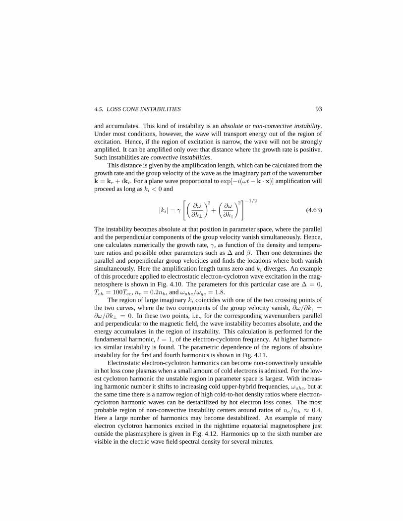
4.5. LOSS CONE INSTABILITIES 93
and accumulates. This kind of instability is anabsoluteor non-convective instability.Under most conditions, however, the wave will transport energy out of the region ofexcitation. Hence, if the region of excitation is narrow, the wave will not be stronglyamplified. It can be amplified only over that distance where the growth rate is positive.Such instabilities areconvective instabilities.
This distance is given by the amplification length, which can be calculated from thegrowth rate and the group velocity of the wave as the imaginary part of the wavenumberk = kr + iki. For a plane wave proportional toexp[−i(ωt− k · x)] amplification willproceed as long aski < 0 and
|ki| = γ
[(∂ω
∂k⊥
)2
+(
∂ω
∂k‖
)2]−1/2
(4.63)
The instability becomes absolute at that position in parameter space, where the paralleland the perpendicular components of the group velocity vanish simultaneously. Hence,one calculates numerically the growth rate,γ, as function of the density and tempera-ture ratios and possible other parameters such as∆ andβ. Then one determines theparallel and perpendicular group velocities and finds the locations where both vanishsimultaneously. Here the amplification length turns zero andki diverges. An exampleof this procedure applied to electrostatic electron-cyclotron wave excitation in the mag-netosphere is shown in Fig. 4.10. The parameters for this particular case are∆ = 0,Teh = 100Tec, nc = 0.2nh, andωuhc/ωge = 1.8.
The region of large imaginaryki coincides with one of the two crossing points ofthe two curves, where the two components of the group velocity vanish,∂ω/∂k‖ =∂ω/∂k⊥ = 0. In these two points, i.e., for the corresponding wavenumbers paralleland perpendicular to the magnetic field, the wave instability becomes absolute, and theenergy accumulates in the region of instability. This calculation is performed for thefundamental harmonic,l = 1, of the electron-cyclotron frequency. At higher harmon-ics similar instability is found. The parametric dependence of the regions of absoluteinstability for the first and fourth harmonics is shown in Fig. 4.11.
Electrostatic electron-cyclotron harmonics can become non-convectively unstablein hot loss cone plasmas when a small amount of cold electrons is admixed. For the low-est cyclotron harmonic the unstable region in parameter space is largest. With increas-ing harmonic number it shifts to increasing cold upper-hybrid frequencies,ωuhc, but atthe same time there is a narrow region of high cold-to-hot density ratios where electron-cyclotron harmonic waves can be destabilized by hot electron loss cones. The mostprobable region of non-convective instability centers around ratios ofnc/nh ≈ 0.4.Here a large number of harmonics may become destabilized. An example of manyelectron cyclotron harmonics excited in the nighttime equatorial magnetosphere justoutside the plasmasphere is given in Fig. 4.12. Harmonics up to the sixth number arevisible in the electric wave field spectral density for several minutes.
94 4. ELECTROSTATIC INSTABILITIES
0
1
10
5 9 ωuhc /ωge
n c/n
h
1
l=4
l=1
Fig. 4.11. Regions of instability for electron-cyclotron harmonics.
Ion-Cyclotron Instability
The cyclotron resonance symmetry between electrons and ions suggests that anelectro-static ion-cyclotron loss cone instabilityshould complement the electrostatic electron-cyclotron instability discussed. This is indeed the case. The technique to determine thenon-convective instability in parameter space is the same as that for the electrostaticelectron-cyclotron waves. The only difference is found in exchanging the hot electronloss cone distribution with the hot ion loss cone distribution in Eq. (I.10.96), but inaddition one must retain the electron contribution to the dielectric response function
ε(ω,k) = 1 +ω2
pe
ω2ge
k2⊥
k2− 1
k2λ2D
Z ′(ζe)
+ω2
pi
k2
∑
l
∞∫
−∞dv‖
Gli(v‖)f0i(v‖, v⊥;∆, β)ω − k‖v‖ − lωgi
= 0 (4.64)
where the dimensionless operator function,Gli, is defined as
Gli = 2π
∫ ∞
0
v⊥dv⊥J2l (k⊥rgi)
[k‖
∂
∂v‖+
lωgi
v⊥
∂
∂v⊥
](4.65)
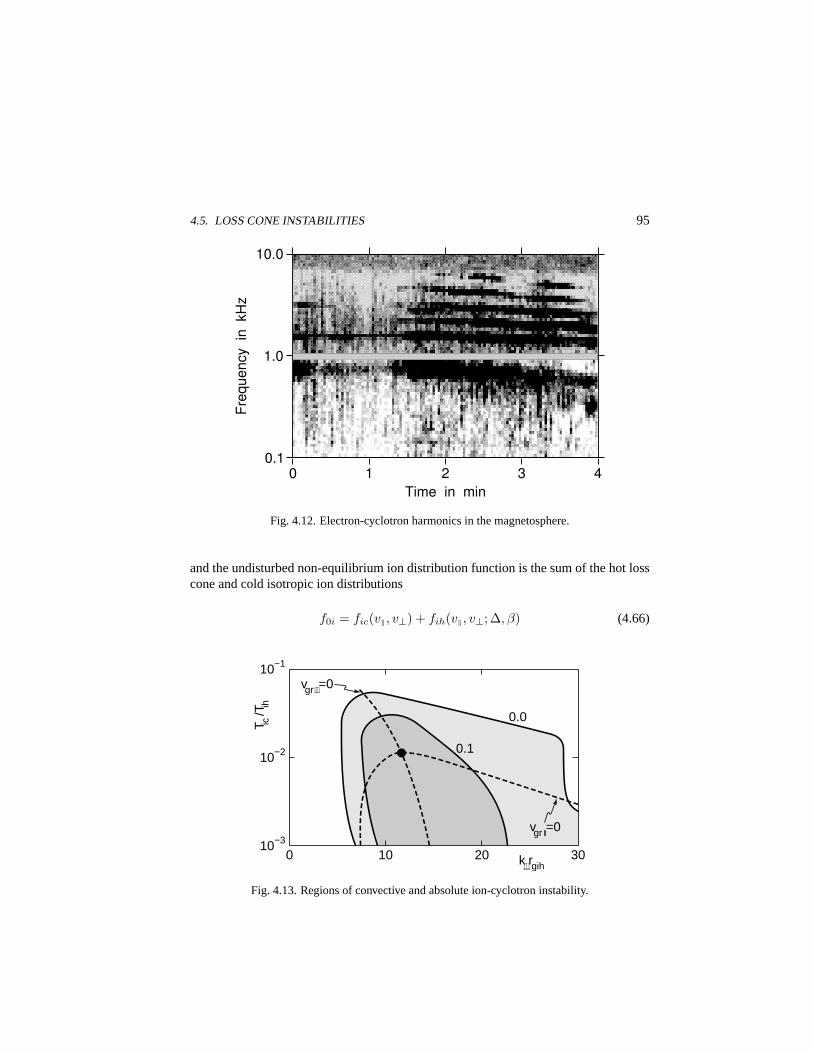
4.5. LOSS CONE INSTABILITIES 95
0.1
1.0
10.0 Fr
eque
ncy
in k
Hz
4 3 2 1 0 Time in min
Fig. 4.12. Electron-cyclotron harmonics in the magnetosphere.
and the undisturbed non-equilibrium ion distribution function is the sum of the hot losscone and cold isotropic ion distributions
f0i = fic(v‖, v⊥) + fih(v‖, v⊥;∆, β) (4.66)
10−3
10−2
10−1
0 10 20 30
T ic/T
ih
k⊥rgih
vgr⊥=0
vgr ||=0
0.0
0.1
Fig. 4.13. Regions of convective and absolute ion-cyclotron instability.
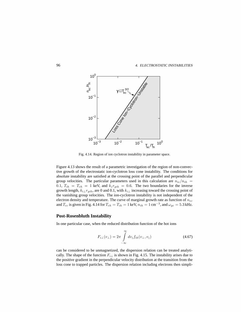
96 4. ELECTROSTATIC INSTABILITIES
10−3
10−2
10−1
100
10−3 10−2 10−1 100
Tec /Tih
n ec/n
ih
γ ∝Tec3/2
Loss
Con
eIo
n−C
yclo
tron−
Uns
tabl
e
Fig. 4.14. Region of ion cyclotron instability in parameter space.
Figure 4.13 shows the result of a parametric investigation of the region of non-convec-tive growth of the electrostatic ion-cyclotron loss cone instability. The conditions forabsolute instability are satisfied at the crossing point of the parallel and perpendiculargroup velocities. The particular parameters used in this calculation arenic/nih =0.1, Tih = Teh = 1 keV, andk‖rgih = 0.6. The two boundaries for the inversegrowth length,ki⊥rgih, are 0 and 0.1, withki⊥ increasing toward the crossing point ofthe vanishing group velocities. The ion-cyclotron instability is not independent of theelectron density and temperature. The curve of marginal growth rate as function ofnec
andTec is given in Fig. 4.14 forTeh = Tih = 1 keV,nih = 1 cm−3, andωge = 5.3 kHz.
Post-Rosenbluth Instability
In one particular case, when the reduced distribution function of the hot ions
Fi⊥(v⊥) = 2π
∞∫
−∞dv‖fih(v⊥, v‖) (4.67)
can be considered to be unmagnetized, the dispersion relation can be treated analyti-cally. The shape of the functionFi⊥ is shown in Fig. 4.15. The instability arises due tothe positive gradient in the perpendicular velocity distribution at the transition from theloss cone to trapped particles. The dispersion relation including electrons then simpli-
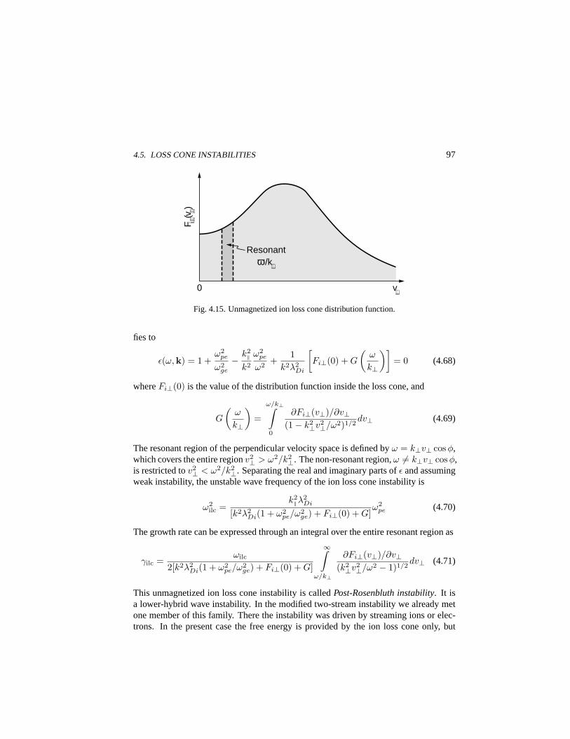
4.5. LOSS CONE INSTABILITIES 97
0
Resonant ω /k⊥
v⊥
F i⊥(v ⊥
)
Fig. 4.15. Unmagnetized ion loss cone distribution function.
fies to
ε(ω,k) = 1 +ω2
pe
ω2ge
− k2‖
k2
ω2pe
ω2+
1k2λ2
Di
[Fi⊥(0) + G
(ω
k⊥
)]= 0 (4.68)
whereFi⊥(0) is the value of the distribution function inside the loss cone, and
G
(ω
k⊥
)=
ω/k⊥∫
0
∂Fi⊥(v⊥)/∂v⊥(1− k2
⊥v2⊥/ω2)1/2
dv⊥ (4.69)
The resonant region of the perpendicular velocity space is defined byω = k⊥v⊥ cos φ,which covers the entire regionv2
⊥ > ω2/k2⊥. The non-resonant region,ω 6= k⊥v⊥ cos φ,
is restricted tov2⊥ < ω2/k2
⊥. Separating the real and imaginary parts ofε and assumingweak instability, the unstable wave frequency of the ion loss cone instability is
ω2ilc =
k2‖λ
2Di
[k2λ2Di(1 + ω2
pe/ω2ge) + Fi⊥(0) + G]
ω2pe (4.70)
The growth rate can be expressed through an integral over the entire resonant region as
γilc =ωilc
2[k2λ2Di(1 + ω2
pe/ω2ge) + Fi⊥(0) + G]
∞∫
ω/k⊥
∂Fi⊥(v⊥)/∂v⊥(k2⊥v2
⊥/ω2 − 1)1/2dv⊥ (4.71)
This unmagnetized ion loss cone instability is calledPost-Rosenbluth instability. It isa lower-hybrid wave instability. In the modified two-stream instability we already metone member of this family. There the instability was driven by streaming ions or elec-trons. In the present case the free energy is provided by the ion loss cone only, but
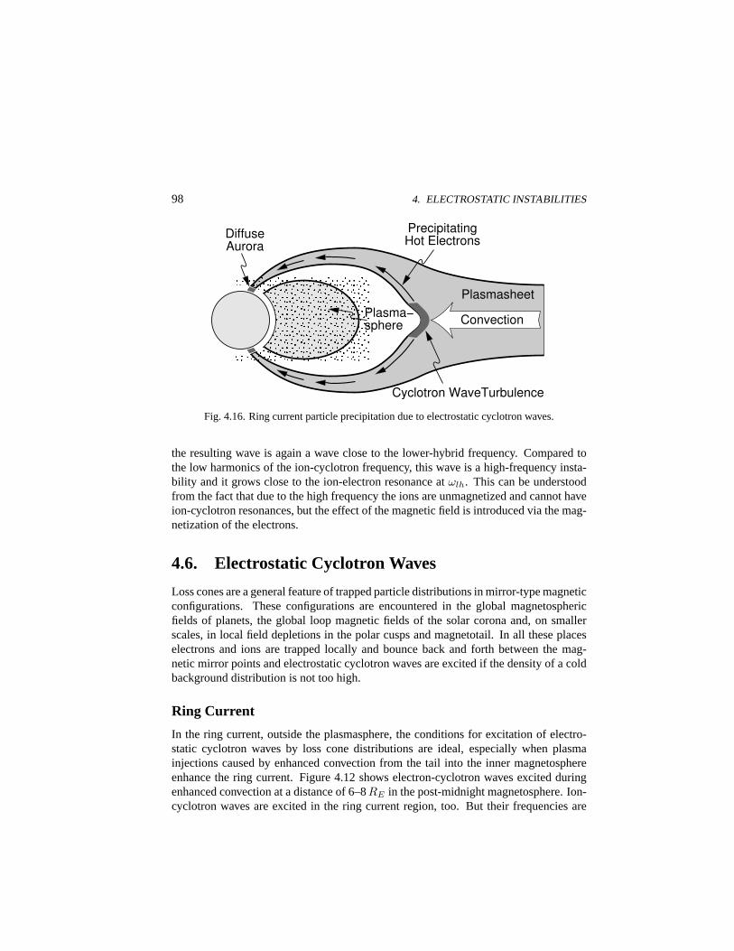
98 4. ELECTROSTATIC INSTABILITIES
Convection Plasma− sphere
Cyclotron WaveTurbulence
Diffuse Aurora
Precipitating Hot Electrons
Plasmasheet
Fig. 4.16. Ring current particle precipitation due to electrostatic cyclotron waves.
the resulting wave is again a wave close to the lower-hybrid frequency. Compared tothe low harmonics of the ion-cyclotron frequency, this wave is a high-frequency insta-bility and it grows close to the ion-electron resonance atωlh. This can be understoodfrom the fact that due to the high frequency the ions are unmagnetized and cannot haveion-cyclotron resonances, but the effect of the magnetic field is introduced via the mag-netization of the electrons.
4.6. Electrostatic Cyclotron Waves
Loss cones are a general feature of trapped particle distributions in mirror-type magneticconfigurations. These configurations are encountered in the global magnetosphericfields of planets, the global loop magnetic fields of the solar corona and, on smallerscales, in local field depletions in the polar cusps and magnetotail. In all these placeselectrons and ions are trapped locally and bounce back and forth between the mag-netic mirror points and electrostatic cyclotron waves are excited if the density of a coldbackground distribution is not too high.
Ring Current
In the ring current, outside the plasmasphere, the conditions for excitation of electro-static cyclotron waves by loss cone distributions are ideal, especially when plasmainjections caused by enhanced convection from the tail into the inner magnetosphereenhance the ring current. Figure 4.12 shows electron-cyclotron waves excited duringenhanced convection at a distance of 6–8RE in the post-midnight magnetosphere. Ion-cyclotron waves are excited in the ring current region, too. But their frequencies are
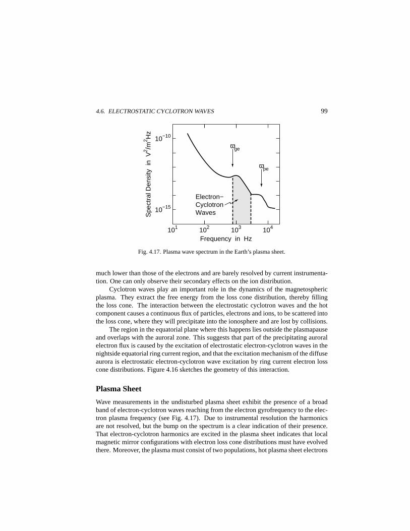
4.6. ELECTROSTATIC CYCLOTRON WAVES 99
ωge
ωpe
10−15
10−10
103 102 101 104
Electron− Cyclotron Waves
Frequency in Hz
Spe
ctra
l Den
sity
in
V2 /m
2 Hz
Fig. 4.17. Plasma wave spectrum in the Earth’s plasma sheet.
much lower than those of the electrons and are barely resolved by current instrumenta-tion. One can only observe their secondary effects on the ion distribution.
Cyclotron waves play an important role in the dynamics of the magnetosphericplasma. They extract the free energy from the loss cone distribution, thereby fillingthe loss cone. The interaction between the electrostatic cyclotron waves and the hotcomponent causes a continuous flux of particles, electrons and ions, to be scattered intothe loss cone, where they will precipitate into the ionosphere and are lost by collisions.
The region in the equatorial plane where this happens lies outside the plasmapauseand overlaps with the auroral zone. This suggests that part of the precipitating auroralelectron flux is caused by the excitation of electrostatic electron-cyclotron waves in thenightside equatorial ring current region, and that the excitation mechanism of the diffuseaurora is electrostatic electron-cyclotron wave excitation by ring current electron losscone distributions. Figure 4.16 sketches the geometry of this interaction.
Plasma Sheet
Wave measurements in the undisturbed plasma sheet exhibit the presence of a broadband of electron-cyclotron waves reaching from the electron gyrofrequency to the elec-tron plasma frequency (see Fig. 4.17). Due to instrumental resolution the harmonicsare not resolved, but the bump on the spectrum is a clear indication of their presence.That electron-cyclotron harmonics are excited in the plasma sheet indicates that localmagnetic mirror configurations with electron loss cone distributions must have evolvedthere. Moreover, the plasma must consist of two populations, hot plasma sheet electrons
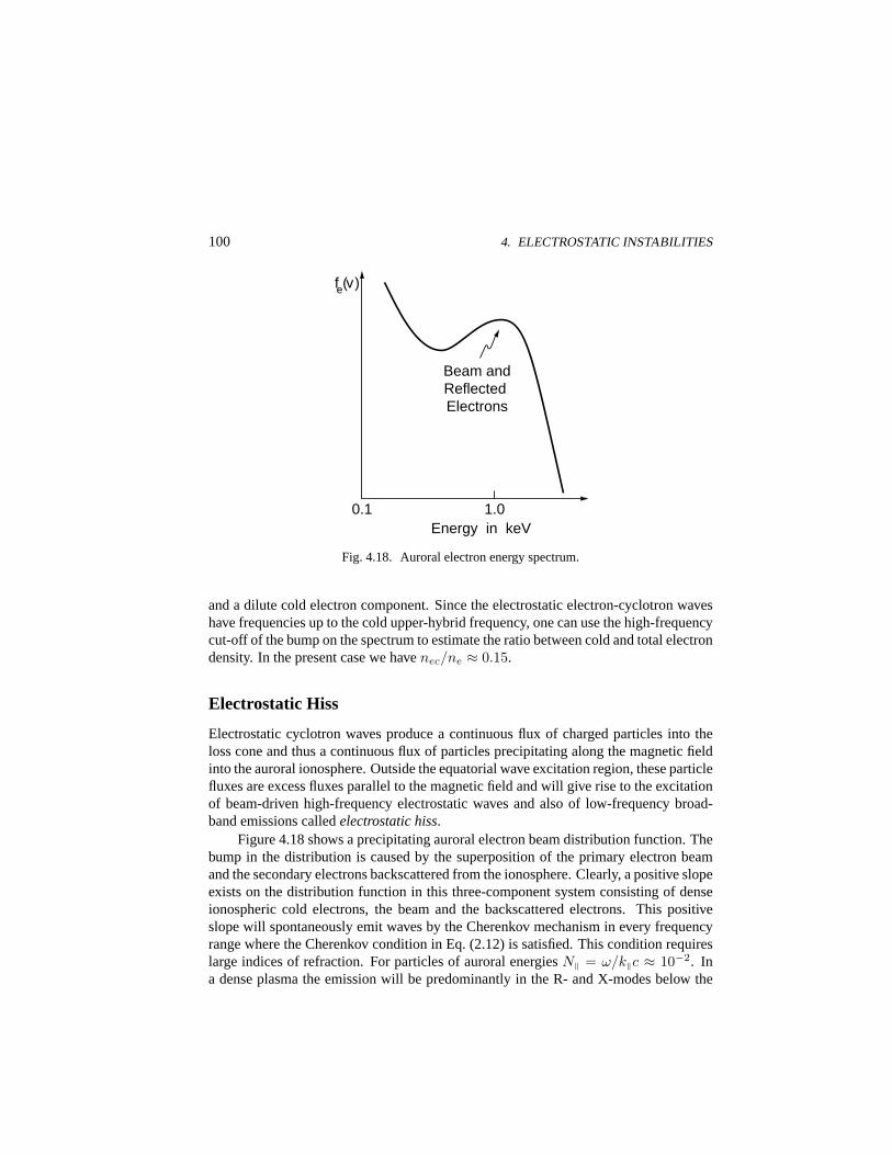
100 4. ELECTROSTATIC INSTABILITIES
Beam and Reflected Electrons
fe(v)
0.1 1.0 Energy in keV
Fig. 4.18. Auroral electron energy spectrum.
and a dilute cold electron component. Since the electrostatic electron-cyclotron waveshave frequencies up to the cold upper-hybrid frequency, one can use the high-frequencycut-off of the bump on the spectrum to estimate the ratio between cold and total electrondensity. In the present case we havenec/ne ≈ 0.15.
Electrostatic Hiss
Electrostatic cyclotron waves produce a continuous flux of charged particles into theloss cone and thus a continuous flux of particles precipitating along the magnetic fieldinto the auroral ionosphere. Outside the equatorial wave excitation region, these particlefluxes are excess fluxes parallel to the magnetic field and will give rise to the excitationof beam-driven high-frequency electrostatic waves and also of low-frequency broad-band emissions calledelectrostatic hiss.
Figure 4.18 shows a precipitating auroral electron beam distribution function. Thebump in the distribution is caused by the superposition of the primary electron beamand the secondary electrons backscattered from the ionosphere. Clearly, a positive slopeexists on the distribution function in this three-component system consisting of denseionospheric cold electrons, the beam and the backscattered electrons. This positiveslope will spontaneously emit waves by the Cherenkov mechanism in every frequencyrange where the Cherenkov condition in Eq. (2.12) is satisfied. This condition requireslarge indices of refraction. For particles of auroral energiesN‖ = ω/k‖c ≈ 10−2. Ina dense plasma the emission will be predominantly in the R- and X-modes below the
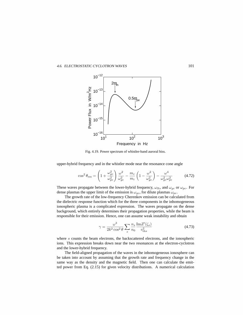
4.6. ELECTROSTATIC CYCLOTRON WAVES 101
2ωlh
103 102 101
Frequency in Hz
0.5ωpe
Pow
er F
lux
in W
/m2 H
z
10−15
10−14
10−13
10−12
10−16
Fig. 4.19. Power spectrum of whistler-band auroral hiss.
upper-hybrid frequency and in the whistler mode near the resonance cone angle
cos2 θres =
(1 +
ω2ge
ω2pe
)ω2
ω2ge
− me
mi
(1− ω2
ω2ge
)− ω4
ω2geω
2pe
(4.72)
These waves propagate between the lower-hybrid frequency,ωlh, andωge or ωpe. Fordense plasmas the upper limit of the emission isωge, for dilute plasmasωpe.
The growth rate of the low-frequency Cherenkov emission can be calculated fromthe dielectric response function which for the three components in the inhomogeneousionospheric plasma is a complicated expression. The waves propagate on the densebackground, which entirely determines their propagation properties, while the beam isresponsible for their emission. Hence, one can assume weak instability and obtain
γ =ω3
2k2 cos2 θ
∑s
ns
n0
ImZ ′(ζs)v2ths
(4.73)
wheres counts the beam electrons, the backscattered electrons, and the ionosphericions. This expression breaks down near the two resonances at the electron-cyclotronand the lower-hybrid frequency.
The field-aligned propagation of the waves in the inhomogeneous ionosphere canbe taken into account by assuming that the growth rate and frequency change in thesame way as the density and the magnetic field. Then one can calculate the emit-ted power from Eq. (2.15) for given velocity distributions. A numerical calculation
102 4. ELECTROSTATIC INSTABILITIES
is shown in Fig. 4.19. The electron beams generate a broad band of electrostatic hissaboveωlh and additional hiss at and aboveωpe. When including more secondaries inthe electrons, the emission maximum is lowered and shifted to higher frequencies.
Concluding Remarks
The microinstabilities discussed in the present chapter are caused by deviations fromthe Maxwellian distribution. However, Maxwellians describe the final state of thermo-dynamic equilibrium of a closed system which is perfectly relaxed. This situation ishardly realized in nature. The normal case will be equilibria between energy inflowand dissipation in a system and the equilibrium distributions will often not resembleideal Maxwellian distributions. Instabilities of various kinds may arise in these equilib-ria, compete dynamically, saturate, and deform the distribution function, causing otherinstabilities to grow and so on. Most of these processes are highly nonlinear, coupledifferent wave modes and affect the motion of the particles.
Further Reading
A number of microinstabilities are reviewed in [1], [4], and [5], where the latter is astandard reference for most of the linear plasma instabilities. Ionospheric instabilitiesare discussed in connection with electrojet theory in [2]. The current-drift velocitythresholds for ion-cyclotron modes were first calculated by Kindel and Kennel,J. Geo-phys. Res. 76 (1971) 3055. The linear and nonlinear theory of electrostatic loss cone-driven cyclotron modes is found in [3]. Cyclotron waves and instabilities are found in[6]. Power spectra of whistler-band auroral hiss were calculated by Maggs,J. Geophys.Res. 34 (1976) 1707, and the plasma sheet wave spectra are from Baumjohann et al.,J.Geophys. Res.95 (1990) 3811.
[1] A. Hasegawa,Plasma Instabilities and Nonlinear Effects(Springer Verlag, Heidel-berg, 1975).
[2] M. C. Kelley,The Earth’s Ionosphere(Academic Press, San Diego, 1989).
[3] C. F. Kennel and M. Ashour-Abdalla, inMagnetospheric Plasma Physics, ed. A.Nishida (D. Reidel Publ. Co., Dordrecht, 1982), p. 245.
[4] D. B. Melrose,Instabilities in Space and Laboratory Plasmas(Cambridge Univer-sity Press, Cambridge, 1991).
[5] A. B. Mikhailovskii, Theory of Plasma Instabilities I(Consultants Bureau, NewYork, 1974).
[6] T. H. Stix,Waves in Plasma(American Institute of Physics, New York, 1992).
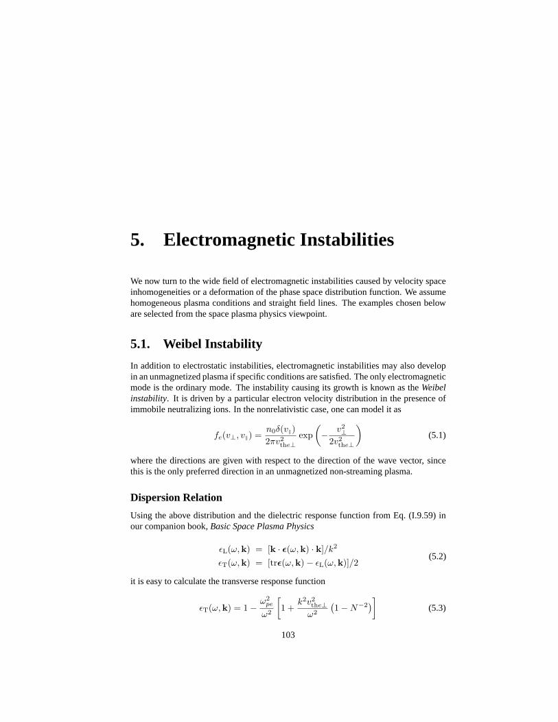
5. Electromagnetic Instabilities
We now turn to the wide field of electromagnetic instabilities caused by velocity spaceinhomogeneities or a deformation of the phase space distribution function. We assumehomogeneous plasma conditions and straight field lines. The examples chosen beloware selected from the space plasma physics viewpoint.
5.1. Weibel Instability
In addition to electrostatic instabilities, electromagnetic instabilities may also developin an unmagnetized plasma if specific conditions are satisfied. The only electromagneticmode is the ordinary mode. The instability causing its growth is known as theWeibelinstability. It is driven by a particular electron velocity distribution in the presence ofimmobile neutralizing ions. In the nonrelativistic case, one can model it as
fe(v⊥, v‖) =n0δ(v‖)2πv2
the⊥exp
(− v2
⊥2v2
the⊥
)(5.1)
where the directions are given with respect to the direction of the wave vector, sincethis is the only preferred direction in an unmagnetized non-streaming plasma.
Dispersion Relation
Using the above distribution and the dielectric response function from Eq. (I.9.59) inour companion book,Basic Space Plasma Physics
εL(ω,k) = [k · ε(ω,k) · k]/k2
εT(ω,k) = [trε(ω,k)− εL(ω,k)]/2(5.2)
it is easy to calculate the transverse response function
εT(ω,k) = 1− ω2pe
ω2
[1 +
k2v2the⊥
ω2
(1−N−2
)](5.3)
103
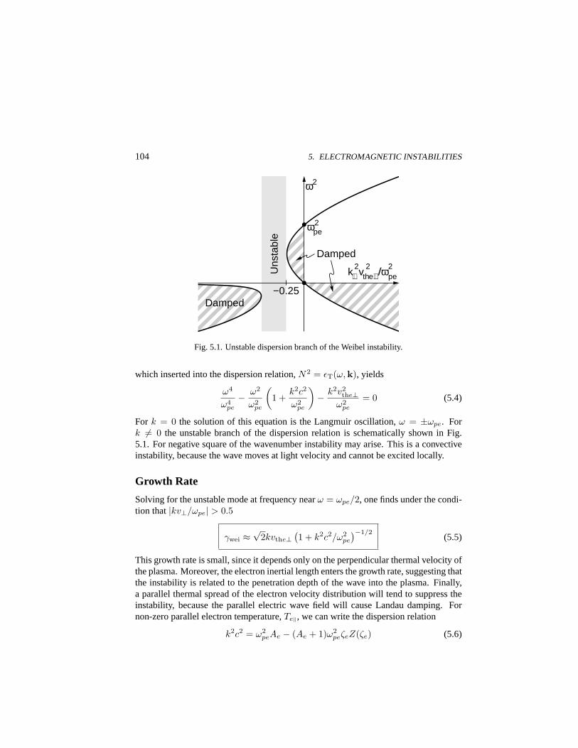
104 5. ELECTROMAGNETIC INSTABILITIES
k⊥2vth
2e⊥/ω2
pe
ω2
ωp2e
Damped
Uns
tabl
e
−0.25 Damped
Fig. 5.1. Unstable dispersion branch of the Weibel instability.
which inserted into the dispersion relation,N2 = εT(ω,k), yields
ω4
ω4pe
− ω2
ω2pe
(1 +
k2c2
ω2pe
)− k2v2
the⊥ω2
pe
= 0 (5.4)
For k = 0 the solution of this equation is the Langmuir oscillation,ω = ±ωpe. Fork 6= 0 the unstable branch of the dispersion relation is schematically shown in Fig.5.1. For negative square of the wavenumber instability may arise. This is a convectiveinstability, because the wave moves at light velocity and cannot be excited locally.
Growth Rate
Solving for the unstable mode at frequency nearω = ωpe/2, one finds under the condi-tion that|kv⊥/ωpe| > 0.5
γwei ≈√
2kvthe⊥(1 + k2c2/ω2
pe
)−1/2(5.5)
This growth rate is small, since it depends only on the perpendicular thermal velocity ofthe plasma. Moreover, the electron inertial length enters the growth rate, suggesting thatthe instability is related to the penetration depth of the wave into the plasma. Finally,a parallel thermal spread of the electron velocity distribution will tend to suppress theinstability, because the parallel electric wave field will cause Landau damping. Fornon-zero parallel electron temperature,Te‖, we can write the dispersion relation
k2c2 = ω2peAe − (Ae + 1)ω2
peζeZ(ζe) (5.6)
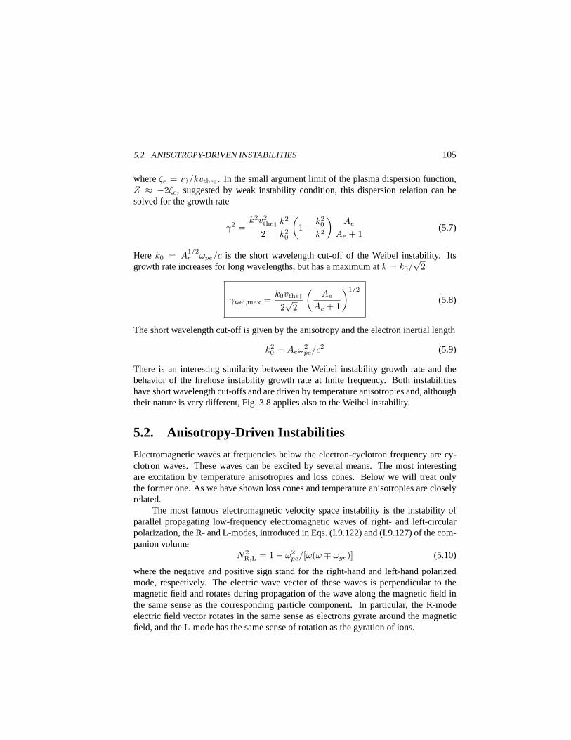
5.2. ANISOTROPY-DRIVEN INSTABILITIES 105
whereζe = iγ/kvthe‖. In the small argument limit of the plasma dispersion function,Z ≈ −2ζe, suggested by weak instability condition, this dispersion relation can besolved for the growth rate
γ2 =k2v2
the‖
2k2
k20
(1− k2
0
k2
)Ae
Ae + 1(5.7)
Herek0 = A1/2e ωpe/c is the short wavelength cut-off of the Weibel instability. Its
growth rate increases for long wavelengths, but has a maximum atk = k0/√
2
γwei,max =k0vthe‖
2√
2
(Ae
Ae + 1
)1/2
(5.8)
The short wavelength cut-off is given by the anisotropy and the electron inertial length
k20 = Aeω
2pe/c2 (5.9)
There is an interesting similarity between the Weibel instability growth rate and thebehavior of the firehose instability growth rate at finite frequency. Both instabilitieshave short wavelength cut-offs and are driven by temperature anisotropies and, althoughtheir nature is very different, Fig. 3.8 applies also to the Weibel instability.
5.2. Anisotropy-Driven Instabilities
Electromagnetic waves at frequencies below the electron-cyclotron frequency are cy-clotron waves. These waves can be excited by several means. The most interestingare excitation by temperature anisotropies and loss cones. Below we will treat onlythe former one. As we have shown loss cones and temperature anisotropies are closelyrelated.
The most famous electromagnetic velocity space instability is the instability ofparallel propagating low-frequency electromagnetic waves of right- and left-circularpolarization, the R- and L-modes, introduced in Eqs. (I.9.122) and (I.9.127) of the com-panion volume
N2R,L = 1− ω2
pe/[ω(ω ∓ ωge)] (5.10)
where the negative and positive sign stand for the right-hand and left-hand polarizedmode, respectively. The electric wave vector of these waves is perpendicular to themagnetic field and rotates during propagation of the wave along the magnetic field inthe same sense as the corresponding particle component. In particular, the R-modeelectric field vector rotates in the same sense as electrons gyrate around the magneticfield, and the L-mode has the same sense of rotation as the gyration of ions.
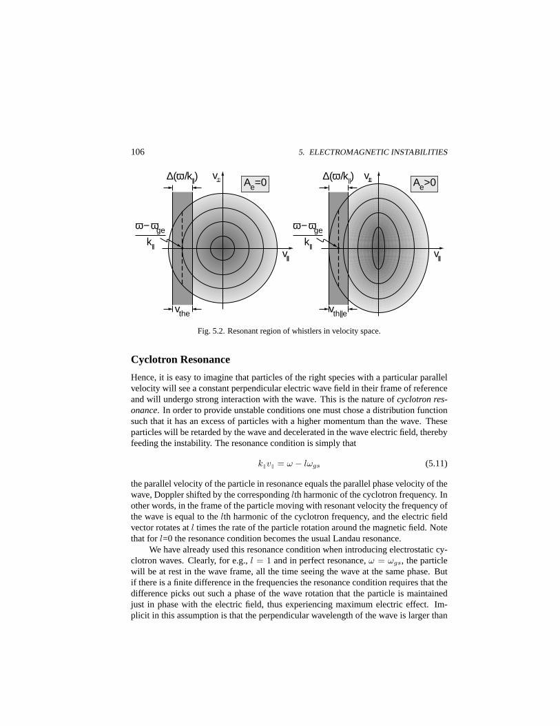
106 5. ELECTROMAGNETIC INSTABILITIES
Ae=0
v||
v⊥
v||
v⊥ ∆(ω /k||)
vthe vth||e
Ae>0 ∆(ω /k||)
ω−ωge
k||
ω−ωge
k||
Fig. 5.2. Resonant region of whistlers in velocity space.
Cyclotron Resonance
Hence, it is easy to imagine that particles of the right species with a particular parallelvelocity will see a constant perpendicular electric wave field in their frame of referenceand will undergo strong interaction with the wave. This is the nature ofcyclotron res-onance. In order to provide unstable conditions one must chose a distribution functionsuch that it has an excess of particles with a higher momentum than the wave. Theseparticles will be retarded by the wave and decelerated in the wave electric field, therebyfeeding the instability. The resonance condition is simply that
k‖v‖ = ω − lωgs (5.11)
the parallel velocity of the particle in resonance equals the parallel phase velocity of thewave, Doppler shifted by the correspondinglth harmonic of the cyclotron frequency. Inother words, in the frame of the particle moving with resonant velocity the frequency ofthe wave is equal to thelth harmonic of the cyclotron frequency, and the electric fieldvector rotates atl times the rate of the particle rotation around the magnetic field. Notethat forl=0 the resonance condition becomes the usual Landau resonance.
We have already used this resonance condition when introducing electrostatic cy-clotron waves. Clearly, for e.g.,l = 1 and in perfect resonance,ω = ωgs, the particlewill be at rest in the wave frame, all the time seeing the wave at the same phase. Butif there is a finite difference in the frequencies the resonance condition requires that thedifference picks out such a phase of the wave rotation that the particle is maintainedjust in phase with the electric field, thus experiencing maximum electric effect. Im-plicit in this assumption is that the perpendicular wavelength of the wave is larger than

5.2. ANISOTROPY-DRIVEN INSTABILITIES 107
z
E
E E
t1, z1
t3, z3
t2, z2
t2, z2
t3, z3
t1, z1
v > ω /k
v < ω /k
Fig. 5.3. Cyclotron resonance mechanism.
the gyroradius of the particles, warranting that the particles are magnetized. But thiscondition is irrelevant for strictly parallel propagation, because then the wave field ishomogeneous in the perpendicular direction with infinite perpendicular wavelength.
The resonance condition is not as easy to understand intuitively as Landau reso-nance. This has to do with the coupling of parallel and perpendicular particle motionin the resonance. Firstly, it cannot be satisfied for arbitrary velocities. For instance,for electron whistlers withl = 1 and no harmonics at largerl, the whistler frequencygiven in Eq. (I.9.125),ωw < ωge, is smaller than the electron-cyclotron frequency, andωw − ωge is negative, implying that electrons in resonance with whistlers propagateopposite to the whistler along the magnetic field.
In a velocity space representation like that of Fig. 5.2, the resonant region is locatedin the negativev‖ plane. For an isotropic Maxwellian plasma withAe = 0 andTe⊥ =Te‖, the isodensity contours of the velocity are circles, and the width of the resonantregion can be estimated to be of the order of the isotropic electron thermal velocity,vthe. For an anisotropic distribution the width is the parallel thermal speed,vthe‖. Inthe isotropic case there is no free energy available and no instability can arise.
The physical mechanism of cyclotron damping and instability is sketched in Fig.5.3. A right-hand circularly polarized wave is moving along the magnetic field, in thez direction. The electric field vector rotates as shown when the wave moves from leftto right. In the electron frame, where the electron is stationary, the wave is passing tothe right if the electron is slow with respect to the wave and to the left if the electronis faster than the wave. A slow electron will see wave vectors in the succession shownby the arrow in the lower part of the figure. Hence, the electric field experienced bythe electron rotates in the same direction as the electron. In this case the electron inresonance will be accelerated by the wave field in the perpendicular direction, leading
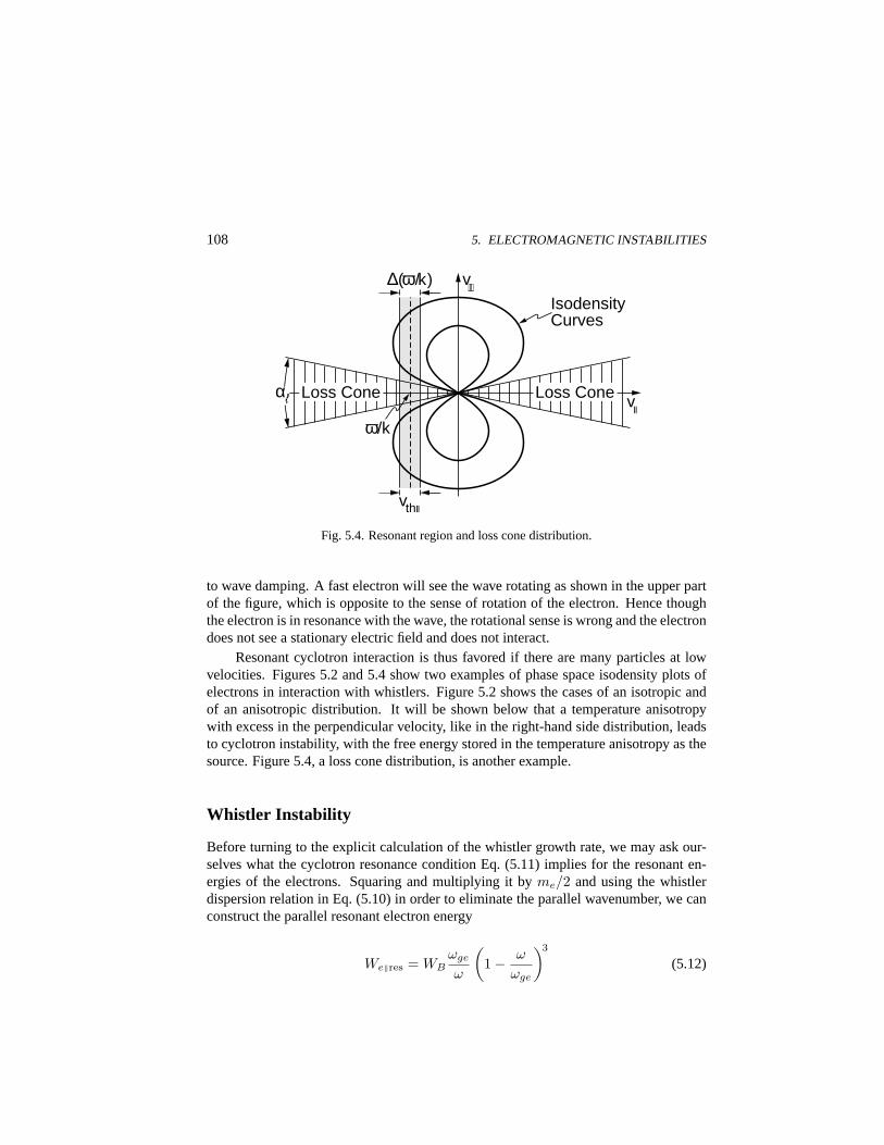
108 5. ELECTROMAGNETIC INSTABILITIES
vll
ω/k
vthll
∆(ω/k) v⊥
Loss Cone Loss Cone
Isodensity Curves
α
Fig. 5.4. Resonant region and loss cone distribution.
to wave damping. A fast electron will see the wave rotating as shown in the upper partof the figure, which is opposite to the sense of rotation of the electron. Hence thoughthe electron is in resonance with the wave, the rotational sense is wrong and the electrondoes not see a stationary electric field and does not interact.
Resonant cyclotron interaction is thus favored if there are many particles at lowvelocities. Figures 5.2 and 5.4 show two examples of phase space isodensity plots ofelectrons in interaction with whistlers. Figure 5.2 shows the cases of an isotropic andof an anisotropic distribution. It will be shown below that a temperature anisotropywith excess in the perpendicular velocity, like in the right-hand side distribution, leadsto cyclotron instability, with the free energy stored in the temperature anisotropy as thesource. Figure 5.4, a loss cone distribution, is another example.
Whistler Instability
Before turning to the explicit calculation of the whistler growth rate, we may ask our-selves what the cyclotron resonance condition Eq. (5.11) implies for the resonant en-ergies of the electrons. Squaring and multiplying it byme/2 and using the whistlerdispersion relation in Eq. (5.10) in order to eliminate the parallel wavenumber, we canconstruct the parallel resonant electron energy
We‖res = WBωge
ω
(1− ω
ωge
)3
(5.12)
5.2. ANISOTROPY-DRIVEN INSTABILITIES 109
where we introduced the magnetic energy per particle,WB = B2/2µ0n. Thus theparticles in resonance with the whistler have a particular parallel energy.
Let us assume that the plasma contains a hot electron component with positivetemperature anisotropy,Ae > 0. This component should be of sufficiently low density,nh ¿ n0, in order to not disturb the propagation of the whistler mode. In such acase the dispersion of the whistler wave is still described by the dispersion relation(I.10.164). In other words, the whistlers propagate on the background of the cold andisotropic plasma component. Since we require this background electron plasma to besufficiently cold, the cyclotron damping term in Eq. (I.10.165) shows that the wavesare practically undamped forvthec → 0. Whistler instability may arise due to the freeenergy stored in the temperature anisotropy of the hot electron component.
Dispersion Relation
Retaining the anisotropy forces allows to use the right-hand dispersion relation of aanisotropic Maxwellian plasma derived in Eq. (I.10.159) of our companion volume
k2‖c
2
ω2= 1 +
∑
s=c,h
ω
k‖vth‖s
ω2ps
ω2
[Z(ζs,1)− k‖vth‖s
ωAesZ
′(ζs,1)]
(5.13)
We need to consider only the imaginary part of this dispersion relation when lookingfor weak growth entirely provided by the hot component. Using the large argumentexpansion of the hot electron plasma dispersion function, the imaginary part of thedispersion relation can be written as
Di(ω, k‖) =√
πω
|k‖|vthh‖
ω2ph
ω2
[1−Ae
(1− ωge
ω
)]exp
[− (ω − ωge)2
k2‖v
2thh‖
](5.14)
The real part of the dispersion relation is taken in its simplified version, since we as-sumed a cold dense background plasma
Dr =k2‖c
2
ω2− 1 +
ω2pc
ω(ω − ωge)(5.15)
Growth Rate
Weak instability is determined by the relationγ = −Di/(∂Dr/∂ω)|γ=0. Performingthe simple algebraic calculations yields the whistler growth rate
γw =
√πω2
ph
|k‖|vthh‖
[1−Ae
(1− ωge
ω
)]exp
[− (ω − ωge)2
k2‖v
2thh‖
][2 +
ω2pcωge
ω(ω − ωge)2
]−1
(5.16)
110 5. ELECTROMAGNETIC INSTABILITIES
Two interesting conclusions can be drawn from this expression. First, since the whistlerfrequency depends on the cold plasma frequency, the growth rate is proportional to theratio of hot-to-cold electron densities,γ ∝ nh/nc. The second and more importantconclusion is that the growth rate is positive only under the condition that
Ae > Aec = ω/(ωge − ω) (5.17)
whereAec is the critical anisotropy for instability. This condition can also be written asa condition on the unstable frequency range for a given anisotropy
ω < ωc = ωgeAe/(Ae + 1) (5.18)
whereωc is the critically unstable frequency. Using this expression in the low-frequencywhistler dispersion relation gives a lower limit on the whistler wavelength
k2‖ < k2
‖c = ω2pcAe/c2 (5.19)
For a given temperature anisotropy of the hot electron distribution function there willalways be an unstable range of frequencies and wavenumbers, which will be excitedand will deplete the temperature anisotropy. Clearly, this frequency range is below theelectron-cyclotron frequency and may be found at very low frequencies. The lowestreasonable frequency, up to which the ion effects can be neglected, is the lower-hybridfrequency,ωlh. Hence, this theory is valid up to anisotropies as small asAe ≈ 0.02.
Threshold
We are now in the position to estimate the lowest threshold for the resonant energy ofthe electrons for instability. Inserting the critical frequency into Eq. (5.12) produces
We‖res >WB
Ae(Ae + 1)2(5.20)
For resonance and instability the electron energy must exceed the limit set by this con-dition. Otherwise instability will be inhibited. Low anisotropies require very highelectron energies to drive whistlers unstable. In the magnetosphere the anisotropies arerelatively low, of the order ofAe ≈ 0.1 − 0.5 in the electron radiation belts and evenlower in the near-Earth plasma sheet.
Parallel energies must thus exceed the Alfven energy several times in order to gen-erate whistlers. But this condition is easily satisfied by the trapped radiation belt particle
5.2. ANISOTROPY-DRIVEN INSTABILITIES 111
component and, under certain favorable conditions, also in the near-Earth plasma sheet.In these regions broadband low-frequency whistler noise is generated and frequentlyobserved as one of the fundamental electromagnetic low-frequency emissions. Thesewaves have a strong effect on the trapped and quasi-trapped particle distributions of theradiation belt and the plasma sheet electrons, leading to enhanced precipitation of hotelectrons during excitation of whistler mode noise due to enhanced anisotropies.
Since enhanced anisotropies are caused by convection of plasma from the tail intothe inner magnetosphere, as we have shown in Eq. (I.2.63) of our companion book,increase of the cross-tail electric field during substorms will often be associated withwhistler mode noise excitation in the near-Earth plasma sheet and enhanced hot electronprecipitation into the diffuse aurora. Similarly, trapping of large amounts of very en-ergetic electrons in the Earth’s radiation belts will also lead to enhanced whistler noisegeneration at lower latitudes and cause radiation belt electrons to precipitate. Hence,whistler mode noise is a very important resonator for anisotropic energetic electrons inthe magnetosphere.
Ion-Cyclotron Waves
An entirely equivalent theory can be developed for the left-hand polarized parallel prop-agating mode at low frequencies, the electromagnetic ion-cyclotron wave. It is easy tofollow the same reasoning as presented for whistlers, using only the different defini-tion of the ion-cyclotron dispersion relation (I.9.140) given in the companion volume,to find that ion-cyclotron waves of frequencyω < ωgi also experience instability inanisotropic hot ion plasmas superimposed on a cold isotropic ion background. Thedispersion relation in this case includes the effect of the electrons and becomes
D(ω, k‖) = 1− k2‖c
2
ω2+
ω2pe
ω2ge
− ω2pe
ωgeω+
+ω2
pi
ω2
ω
k‖vthiZ(ζi) + Ai [1 + ζiZ(ζi)]
(5.21)
whereζi = (ω − ωi)/k‖vthi and charge neutrality requires that
ω2pe
ωge= −ω2
pi
ωgi(5.22)
When neglecting the effect of the electrons, the solution to this dispersion relation sim-ply parallels that of the electron whistler case. Ion-cyclotron instability driven by tem-perature anisotropies of hot ions is found in the frequency range
ω < ωc = ωgiAi/(Ai + 1) (5.23)
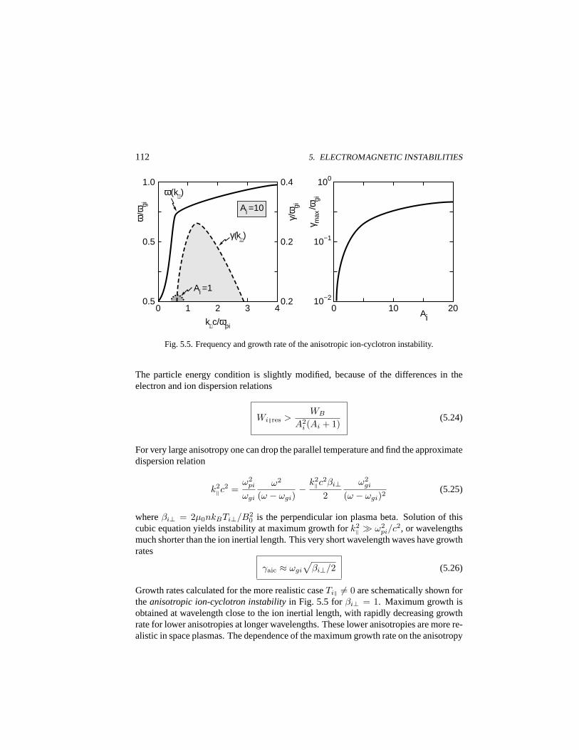
112 5. ELECTROMAGNETIC INSTABILITIES
ω(k⊥)
Ai =10
γ/ω gi
0.2
0.4
0.2 1 3 0 2 4
k⊥c/ωpi
0 10 20 Ai
Ai =1
γ(k⊥) 0.5
1.0
ω/ω
gi
0.5 γ m
ax/ω
gi
10−1
100
10−2
Fig. 5.5. Frequency and growth rate of the anisotropic ion-cyclotron instability.
The particle energy condition is slightly modified, because of the differences in theelectron and ion dispersion relations
Wi‖res >WB
A2i (Ai + 1)
(5.24)
For very large anisotropy one can drop the parallel temperature and find the approximatedispersion relation
k2‖c
2 =ω2
pi
ωgi
ω2
(ω − ωgi)− k2
‖c2βi⊥2
ω2gi
(ω − ωgi)2(5.25)
whereβi⊥ = 2µ0nkBTi⊥/B20 is the perpendicular ion plasma beta. Solution of this
cubic equation yields instability at maximum growth fork2‖ À ω2
pi/c2, or wavelengthsmuch shorter than the ion inertial length. This very short wavelength waves have growthrates
γaic ≈ ωgi
√βi⊥/2 (5.26)
Growth rates calculated for the more realistic caseTi‖ 6= 0 are schematically shown fortheanisotropic ion-cyclotron instabilityin Fig. 5.5 forβi⊥ = 1. Maximum growth isobtained at wavelength close to the ion inertial length, with rapidly decreasing growthrate for lower anisotropies at longer wavelengths. These lower anisotropies are more re-alistic in space plasmas. The dependence of the maximum growth rate on the anisotropy
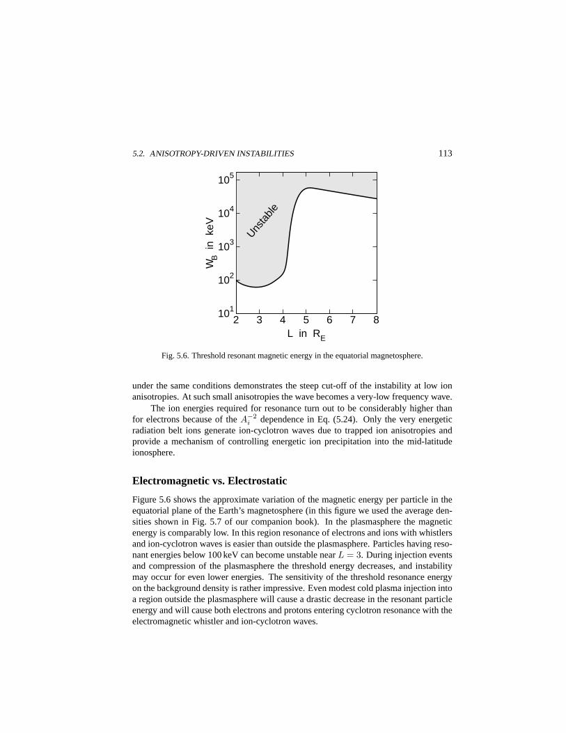
5.2. ANISOTROPY-DRIVEN INSTABILITIES 113
L in RE
101
2 3 4 5 6 7 8
102
103
104
105
WB i
n k
eV
Unsta
ble
Fig. 5.6. Threshold resonant magnetic energy in the equatorial magnetosphere.
under the same conditions demonstrates the steep cut-off of the instability at low ionanisotropies. At such small anisotropies the wave becomes a very-low frequency wave.
The ion energies required for resonance turn out to be considerably higher thanfor electrons because of theA−2
i dependence in Eq. (5.24). Only the very energeticradiation belt ions generate ion-cyclotron waves due to trapped ion anisotropies andprovide a mechanism of controlling energetic ion precipitation into the mid-latitudeionosphere.
Electromagnetic vs. Electrostatic
Figure 5.6 shows the approximate variation of the magnetic energy per particle in theequatorial plane of the Earth’s magnetosphere (in this figure we used the average den-sities shown in Fig. 5.7 of our companion book). In the plasmasphere the magneticenergy is comparably low. In this region resonance of electrons and ions with whistlersand ion-cyclotron waves is easier than outside the plasmasphere. Particles having reso-nant energies below 100 keV can become unstable nearL = 3. During injection eventsand compression of the plasmasphere the threshold energy decreases, and instabilitymay occur for even lower energies. The sensitivity of the threshold resonance energyon the background density is rather impressive. Even modest cold plasma injection intoa region outside the plasmasphere will cause a drastic decrease in the resonant particleenergy and will cause both electrons and protons entering cyclotron resonance with theelectromagnetic whistler and ion-cyclotron waves.
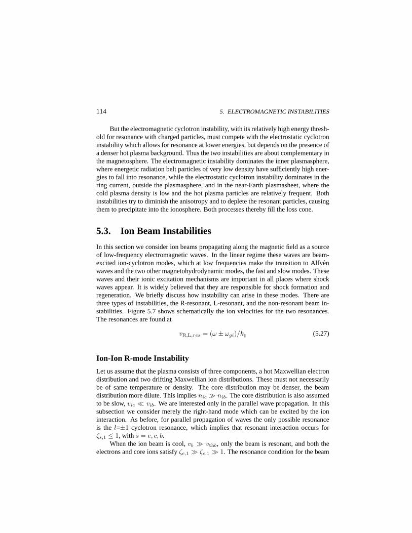
114 5. ELECTROMAGNETIC INSTABILITIES
But the electromagnetic cyclotron instability, with its relatively high energy thresh-old for resonance with charged particles, must compete with the electrostatic cyclotroninstability which allows for resonance at lower energies, but depends on the presence ofa denser hot plasma background. Thus the two instabilities are about complementary inthe magnetosphere. The electromagnetic instability dominates the inner plasmasphere,where energetic radiation belt particles of very low density have sufficiently high ener-gies to fall into resonance, while the electrostatic cyclotron instability dominates in thering current, outside the plasmasphere, and in the near-Earth plasmasheet, where thecold plasma density is low and the hot plasma particles are relatively frequent. Bothinstabilities try to diminish the anisotropy and to deplete the resonant particles, causingthem to precipitate into the ionosphere. Both processes thereby fill the loss cone.
5.3. Ion Beam Instabilities
In this section we consider ion beams propagating along the magnetic field as a sourceof low-frequency electromagnetic waves. In the linear regime these waves are beam-excited ion-cyclotron modes, which at low frequencies make the transition to Alfvenwaves and the two other magnetohydrodynamic modes, the fast and slow modes. Thesewaves and their ionic excitation mechanisms are important in all places where shockwaves appear. It is widely believed that they are responsible for shock formation andregeneration. We briefly discuss how instability can arise in these modes. There arethree types of instabilities, the R-resonant, L-resonant, and the non-resonant beam in-stabilities. Figure 5.7 shows schematically the ion velocities for the two resonances.The resonances are found at
vR,L,res = (ω ± ωgi)/k‖ (5.27)
Ion-Ion R-mode Instability
Let us assume that the plasma consists of three components, a hot Maxwellian electrondistribution and two drifting Maxwellian ion distributions. These must not necessarilybe of same temperature or density. The core distribution may be denser, the beamdistribution more dilute. This impliesnic À nib. The core distribution is also assumedto be slow,vic ¿ vib. We are interested only in the parallel wave propagation. In thissubsection we consider merely the right-hand mode which can be excited by the ioninteraction. As before, for parallel propagation of waves the only possible resonanceis the l=±1 cyclotron resonance, which implies that resonant interaction occurs forζs,1 ≤ 1, with s = e, c, b.
When the ion beam is cool,vb À vthb, only the beam is resonant, and both theelectrons and core ions satisfyζe,1 À ζc,1 À 1. The resonance condition for the beam
5.3. ION BEAM INSTABILITIES 115
f (v||)
vL,res vR,res
fic
fib
v||
Fig. 5.7. Ion beam resonances with R- and L-modes.
with the R-mode is
ω = k‖vb − ωgi (5.28)
and the mode propagates along the beam withk‖ > 0. The growth rate for this insta-bility is found numerically to be of the order of the frequency,γ ≈ ω. The real part ofthe dispersion relation under these conditions is
k2c2
ω2= 1−
∑s
ω2ps(ω − k‖vsb)
ω2(ω ± ωgs − k‖vsb)(5.29)
and the weakly unstable growth rate for drifting Maxwellians is obtained by replacingω → ω − k‖vsb in the imaginary part of the dispersion relation. This yields
γ = ω
√π
2
∑s
ω2ps
ω2
(vsb
vths− ω
k‖vths
)exp
[− (ω ± ωgs − k‖vsb)2
k2‖v
2ths
](5.30)
Under the above assumptions and forvib À vA, the maximum growth rate is
γiib,max = ωgi
(nb
2n0
)1/3
(5.31)
This electromagneticion-ion beam R-mode instabilityresembles the electrostatic beaminstability in Eq. (2.37). Wave growth is obtained above a threshold beam speed of
vib ≥ vA (5.32)
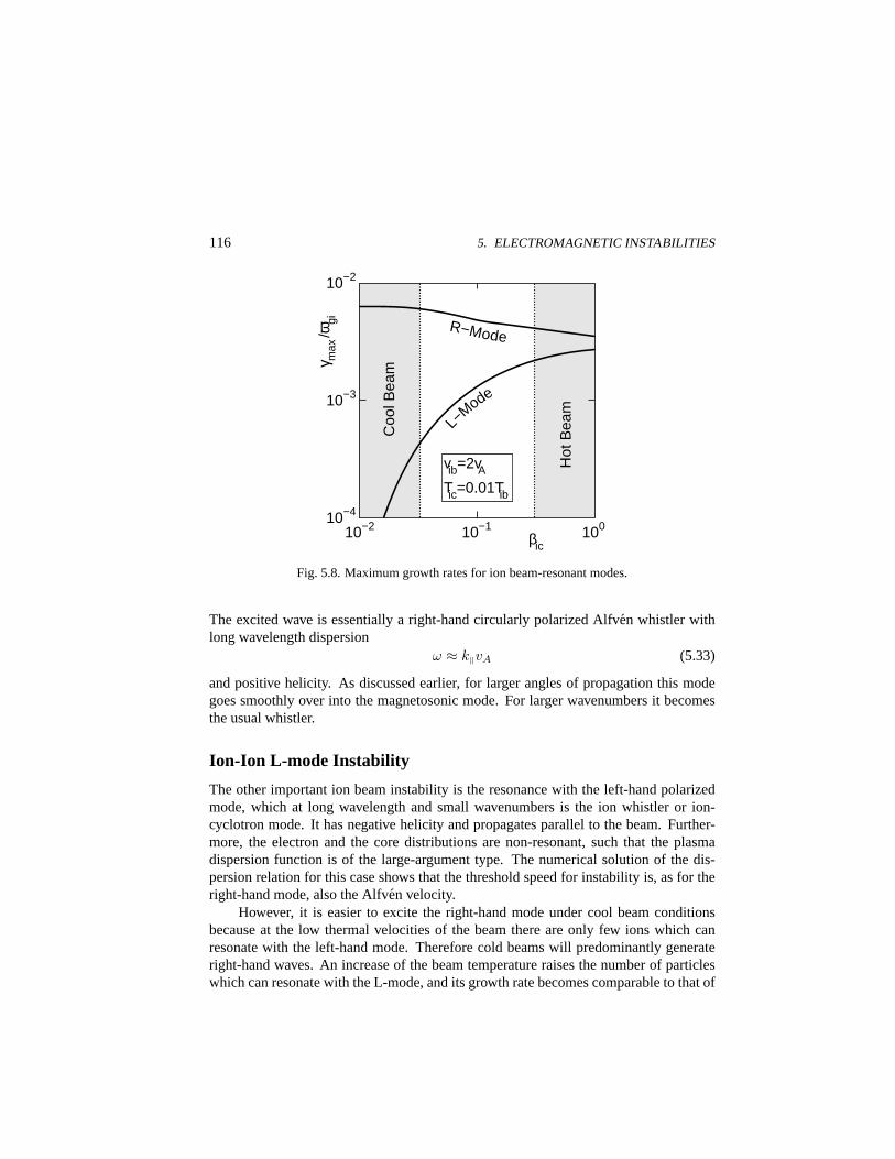
116 5. ELECTROMAGNETIC INSTABILITIES
L−Mode
R−Mode
Coo
l Bea
m
Hot
Bea
m
10−4
10−3
10−2
γ max
/ωgi
10−2 10−1 100 βic
vib=2vA
Tic=0.01Tib
Fig. 5.8. Maximum growth rates for ion beam-resonant modes.
The excited wave is essentially a right-hand circularly polarized Alfven whistler withlong wavelength dispersion
ω ≈ k‖vA (5.33)
and positive helicity. As discussed earlier, for larger angles of propagation this modegoes smoothly over into the magnetosonic mode. For larger wavenumbers it becomesthe usual whistler.
Ion-Ion L-mode Instability
The other important ion beam instability is the resonance with the left-hand polarizedmode, which at long wavelength and small wavenumbers is the ion whistler or ion-cyclotron mode. It has negative helicity and propagates parallel to the beam. Further-more, the electron and the core distributions are non-resonant, such that the plasmadispersion function is of the large-argument type. The numerical solution of the dis-persion relation for this case shows that the threshold speed for instability is, as for theright-hand mode, also the Alfven velocity.
However, it is easier to excite the right-hand mode under cool beam conditionsbecause at the low thermal velocities of the beam there are only few ions which canresonate with the left-hand mode. Therefore cold beams will predominantly generateright-hand waves. An increase of the beam temperature raises the number of particleswhich can resonate with the L-mode, and its growth rate becomes comparable to that of
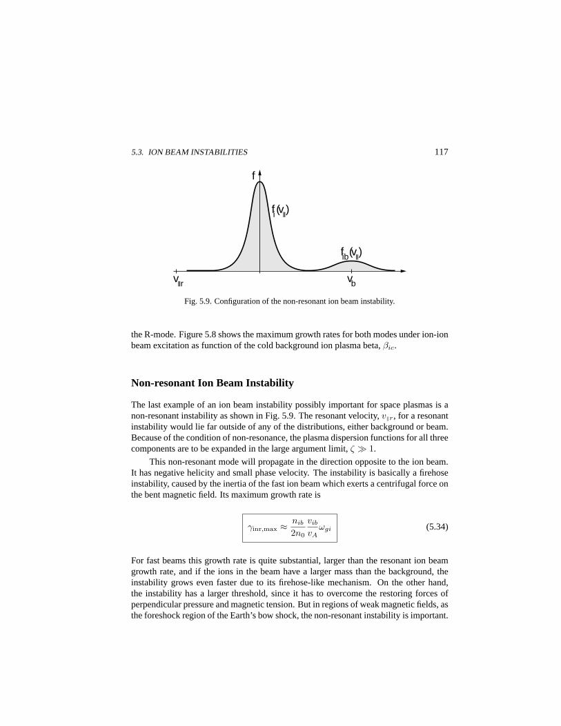
5.3. ION BEAM INSTABILITIES 117
f
fi (vll)
fib(vll)
vb vllr
Fig. 5.9. Configuration of the non-resonant ion beam instability.
the R-mode. Figure 5.8 shows the maximum growth rates for both modes under ion-ionbeam excitation as function of the cold background ion plasma beta,βic.
Non-resonant Ion Beam Instability
The last example of an ion beam instability possibly important for space plasmas is anon-resonant instability as shown in Fig. 5.9. The resonant velocity,v‖r, for a resonantinstability would lie far outside of any of the distributions, either background or beam.Because of the condition of non-resonance, the plasma dispersion functions for all threecomponents are to be expanded in the large argument limit,ζ À 1.
This non-resonant mode will propagate in the direction opposite to the ion beam.It has negative helicity and small phase velocity. The instability is basically a firehoseinstability, caused by the inertia of the fast ion beam which exerts a centrifugal force onthe bent magnetic field. Its maximum growth rate is
γinr,max ≈ nib
2n0
vib
vAωgi (5.34)
For fast beams this growth rate is quite substantial, larger than the resonant ion beamgrowth rate, and if the ions in the beam have a larger mass than the background, theinstability grows even faster due to its firehose-like mechanism. On the other hand,the instability has a larger threshold, since it has to overcome the restoring forces ofperpendicular pressure and magnetic tension. But in regions of weak magnetic fields, asthe foreshock region of the Earth’s bow shock, the non-resonant instability is important.
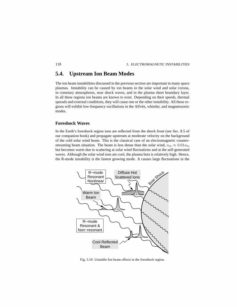
118 5. ELECTROMAGNETIC INSTABILITIES
5.4. Upstream Ion Beam Modes
The ion beam instabilities discussed in the previous section are important in many spaceplasmas. Instability can be caused by ion beams in the solar wind and solar corona,in cometary atmospheres, near shock waves, and in the plasma sheet boundary layer.In all these regions ion beams are known to exist. Depending on their speeds, thermalspreads and external conditions, they will cause one or the other instability. All these re-gions will exhibit low-frequency oscillations in the Alfven, whistler, and magnetosonicmodes.
Foreshock Waves
In the Earth’s foreshock region ions are reflected from the shock front (see Sec. 8.5 ofour companion book) and propagate upstream at moderate velocity on the backgroundof the cold solar wind beam. This is the classical case of an electromagnetic counter-streaming beam situation. The beam is less dense than the solar wind,nib ≈ 0.01n0,but becomes warm due to scattering at solar wind fluctuations and at the self-generatedwaves. Although the solar wind ions are cool, the plasma beta is relatively high. Hence,the R-mode instability is the fastest growing mode. It causes large fluctuations in the
BowShock
Cool Reflected Beam
Diffuse Hot Scattered Ions
R−mode Resonant &
Non−resonant
Warm Ion Beam
R−mode Resonant Nonlinear
Fig. 5.10. Unstable Ion beam effects in the foreshock region.
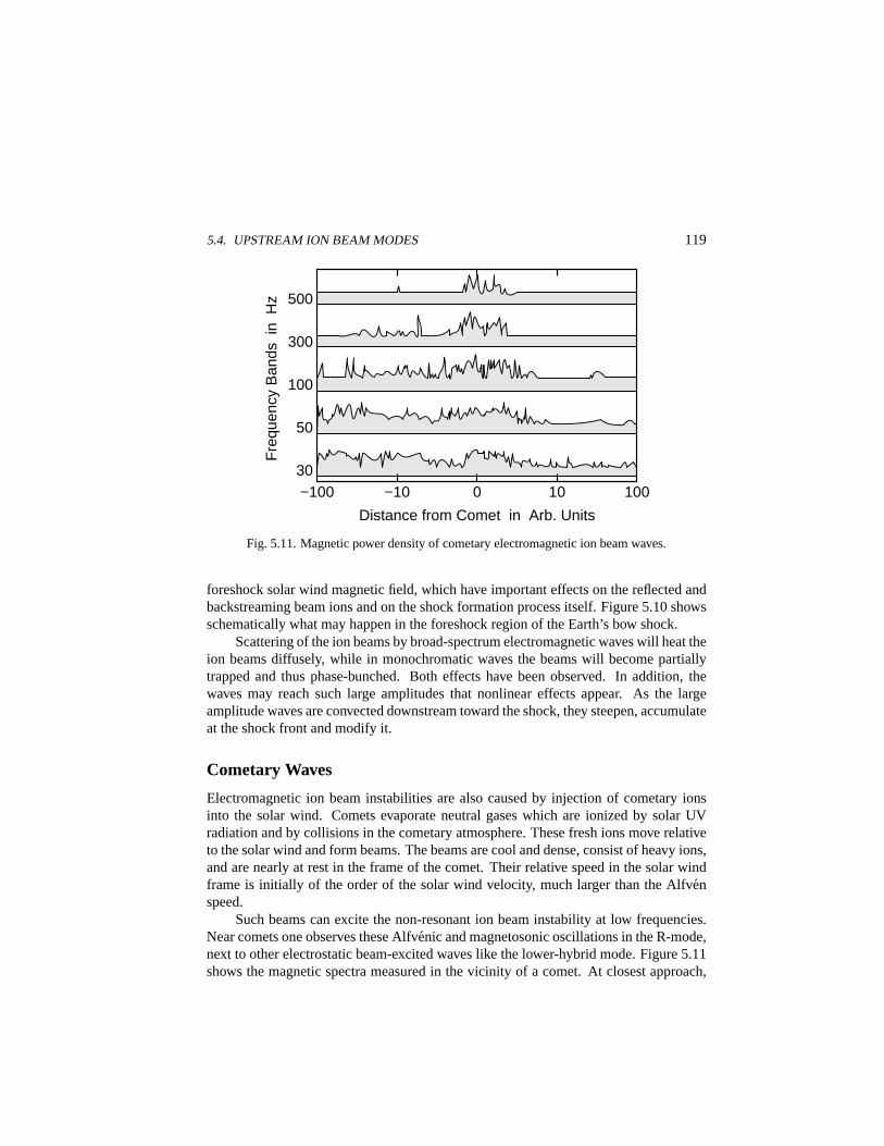
5.4. UPSTREAM ION BEAM MODES 119
30
50
100
300
500
−100 −10 0 10 100
Distance from Comet in Arb. Units
Fre
quen
cy B
ands
in
Hz
Fig. 5.11. Magnetic power density of cometary electromagnetic ion beam waves.
foreshock solar wind magnetic field, which have important effects on the reflected andbackstreaming beam ions and on the shock formation process itself. Figure 5.10 showsschematically what may happen in the foreshock region of the Earth’s bow shock.
Scattering of the ion beams by broad-spectrum electromagnetic waves will heat theion beams diffusely, while in monochromatic waves the beams will become partiallytrapped and thus phase-bunched. Both effects have been observed. In addition, thewaves may reach such large amplitudes that nonlinear effects appear. As the largeamplitude waves are convected downstream toward the shock, they steepen, accumulateat the shock front and modify it.
Cometary Waves
Electromagnetic ion beam instabilities are also caused by injection of cometary ionsinto the solar wind. Comets evaporate neutral gases which are ionized by solar UVradiation and by collisions in the cometary atmosphere. These fresh ions move relativeto the solar wind and form beams. The beams are cool and dense, consist of heavy ions,and are nearly at rest in the frame of the comet. Their relative speed in the solar windframe is initially of the order of the solar wind velocity, much larger than the Alfvenspeed.
Such beams can excite the non-resonant ion beam instability at low frequencies.Near comets one observes these Alfvenic and magnetosonic oscillations in the R-mode,next to other electrostatic beam-excited waves like the lower-hybrid mode. Figure 5.11shows the magnetic spectra measured in the vicinity of a comet. At closest approach,
120 5. ELECTROMAGNETIC INSTABILITIES
where the newly injected ion density is highest, one sees strong magnetic emissions inthe Alfven and whistler bands.
5.5. Maser Instability
Propagating plasma waves contribute to redistribution of energy and to transport ofinformation. The various instabilities discussed so far generate waves which are trappedin the plasma. But there is also radiation which can escape from the plasma. Suchradiation is observed from natural plasmas, like the solar corona, magnetized stars, thelarge planets like Jupiter, and also from the magnetosphere. Radiation is emitted byaccelerated electrons moving in the curved magnetic field. This gyro or synchrotronradiation requires highly energetic electrons, which exist only in the radiation belts.
However, there is also nonthermal radiation like theauroral kilometric radiationobserved in the magnetosphere during substorms. Auroral kilometric radiation is veryimpulsive and intense and cannot be generated as gyro-emission from trapped particles.Thus one needs a linear excitation mechanism, an instability in either the O-mode orthe X-mode. Mechanisms of this kind can exist only under extreme plasma conditions,because the escaping branches of both modes propagate at very high speeds and there-fore need very long amplification lengths to reach reasonable amplitudes and requirerelativistic electrons to interact with.
Relativistic electrons modify the resonant orbits in the (v‖, v⊥) plane and favorresonance with one of the escaping modes. Numerically, a strong instability can be ob-tained if the weakly relativistic electron distribution has a loss cone. Such distributionsare common in magnetospheres, in the solar atmosphere, and in mirror-type magneticfield configuration. That the electrons have to be relativistic is only a weak restriction.Even 10 keV electrons are sufficiently relativistic to yield an instability. Also weaklyrelativistic parallel electron beams, as observed in the aurora, are capable of direct am-plification of the escaping modes.
In effect, the physical mechanism of the direct electromagnetic mode instabilityis an inversion of the absorption coefficient of the plasma by the combination of therelativistic effect and the presence of the loss cone. The excess energy stored in theparticles outside the loss cone and the positive gradient in the perpendicular velocitydistribution of the particles are responsible for this turn-around. Because of this reasonthe plasma starts behaving not as an absorber but as a nearly coherent emitter. This isthe reason why one is speaking of acyclotron maser instability.
Cyclotron Emissions
All mechanisms of direct cyclotron radiation are based on linear instability of theplasma in one of the free space modes. Such instabilities depend on the resonance
5.5. MASER INSTABILITY 121
conditionk‖v‖ − ω + lωge = 0 (5.35)
where only the electron-cyclotron frequency enters for the high-frequency modes. Theions serve as a neutralizing background, as was the case for the solutions of the disper-sion relation (I.9.115) given in the companion volume. The above resonance conditioncontains resonances at all harmonics. Thel=0 resonance is the Cherenkov resonance,which requiresN2 cos2 θ = k2
‖c2/ω2 > 1 for emission and thus very fast particles.
Electrostatic Cherenkov emission (see Secs. 2.1 and 4.6) is of no interest here, but thel=0 resonance for parallel or oblique propagation will always cause Landau damping.
Cyclotron emission is obtained forω ≈ lωge À |k‖v‖|. Actually, this condition isappropriate for escaping waves, because for these wavesN2 < 1 and thus for nonrel-ativistic particlesk‖v‖ = N(v‖/c)ω cos θ ¿ 1. For nonrelativistic resonant particlesleading to emission of waves one speaks ofcyclotron emission, mildly relativistic parti-cles producegyro-emission, and ultra-relativistic particles lead tosynchrotron emission.In both relativistic cases the relativistic dependence of the cyclotron frequency on thevelocity must be taken into account. This requires redefinition ofωge
ωge → ωge/γR (5.36)
The right-hand side contains the relativistic gamma factor
γR =(1− v2/c2
)−1/2(5.37)
which shows that the resonance condition (5.35) becomes a complicated function ofboth components of the particle velocity, which implies that it now describes a fullres-onance curvein the velocity plane. The straight resonance strips of the low-frequencyR- and L-modes thereby deform into resonance regions for the high-frequency modes.
For mildly relativistic electronsγR can be expanded, and Eq. (5.35) states that
k‖v‖ − ω + lωge
[1− (v2
‖ + v2⊥)/2c2
]= 0 (5.38)
which is a quadratic equation for the resonant frequency. One obtains two resonantvalues forv‖ depending onv⊥, instead of the single nonrelativistic resonance,v‖ =(ω− lωge)/k‖. Sincev/c < 1, the physical solutions of the resonance condition are re-stricted to the region inside a circle of radiusv/c in the(v‖/c, v⊥/c) plane. To identifythe curve described by the above resonance condition, we rewrite it as
v2⊥
c2+
(v‖ − k‖c2/lωge)2
c2=
v2r
c2(5.39)
In three-dimensional velocity space this equation describes a sphere centered atvc⊥ =0 andvc‖/c = k‖c/lωge with radius
vr
c=
vc‖
c
[1− 2c2(ω − lωge)
lωgev2c‖
]1/2
(5.40)
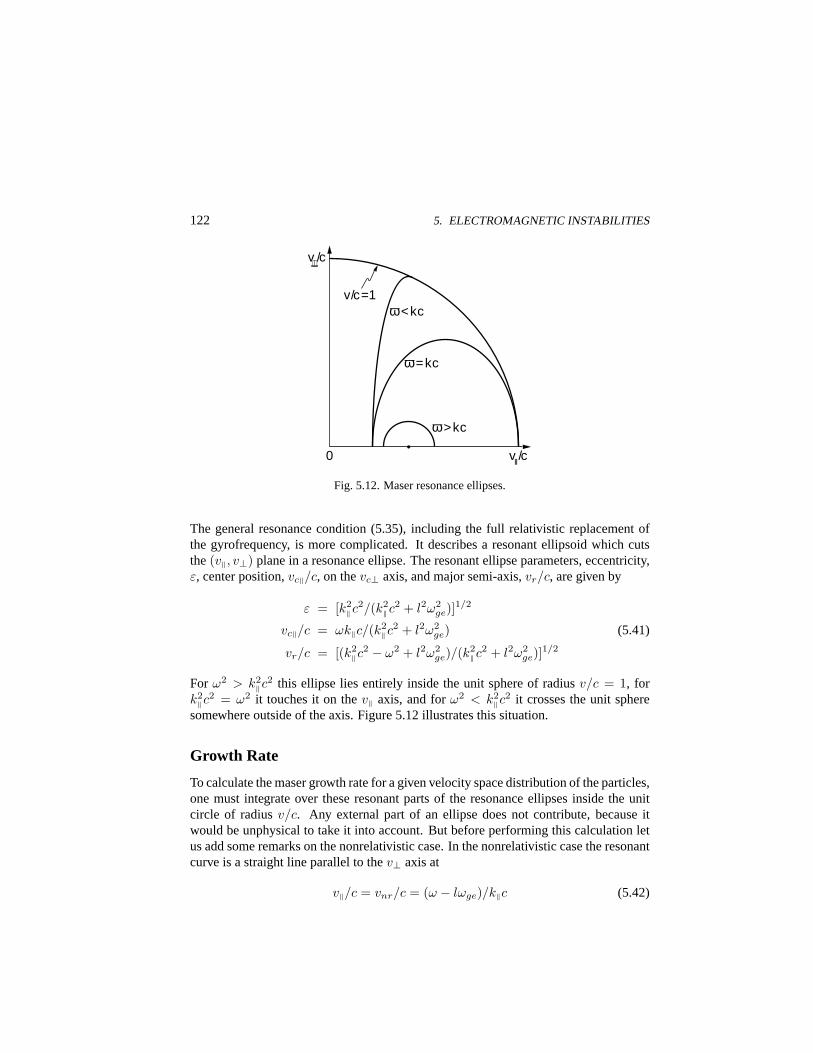
122 5. ELECTROMAGNETIC INSTABILITIES
vll/c
v⊥/c
0
ω <kc
ω =kc
ω >kc
v/c=1
Fig. 5.12. Maser resonance ellipses.
The general resonance condition (5.35), including the full relativistic replacement ofthe gyrofrequency, is more complicated. It describes a resonant ellipsoid which cutsthe(v‖, v⊥) plane in a resonance ellipse. The resonant ellipse parameters, eccentricity,ε, center position,vc‖/c, on thevc⊥ axis, and major semi-axis,vr/c, are given by
ε = [k2‖c
2/(k2‖c
2 + l2ω2ge)]
1/2
vc‖/c = ωk‖c/(k2‖c
2 + l2ω2ge) (5.41)
vr/c = [(k2‖c
2 − ω2 + l2ω2ge)/(k2
‖c2 + l2ω2
ge)]1/2
For ω2 > k2‖c
2 this ellipse lies entirely inside the unit sphere of radiusv/c = 1, fork2‖c
2 = ω2 it touches it on thev‖ axis, and forω2 < k2‖c
2 it crosses the unit spheresomewhere outside of the axis. Figure 5.12 illustrates this situation.
Growth Rate
To calculate the maser growth rate for a given velocity space distribution of the particles,one must integrate over these resonant parts of the resonance ellipses inside the unitcircle of radiusv/c. Any external part of an ellipse does not contribute, because itwould be unphysical to take it into account. But before performing this calculation letus add some remarks on the nonrelativistic case. In the nonrelativistic case the resonantcurve is a straight line parallel to thev⊥ axis at
v‖/c = vnr/c = (ω − lωge)/k‖c (5.42)
5.5. MASER INSTABILITY 123
This straight line is a tangent to one of the ellipses in the resonant plane at smallv‖and, of course, also for smallv⊥. But sincevnr must be nonrelativistic, one requires inaddition that the relativistic shift of the center of the resonant curve must be large so that|vc‖| ≈ vr À |vnr| ≈ |vr−vc‖|. That this tangent is not a good approximation in manycases is immediately obvious from the shapes of the resonance curves. Moreover, theintegration in the nonrelativistic case is performed along this straight line up to infinity,where the resonance curve has long deviated from it.
In the mildly relativistic case, when one integrates along the shifted-circle reso-nance curve, integration is performed only over a limited range of perpendicular veloc-ities,v⊥ < vr. Let us write the variables of integration along the resonant circle as
v‖ = vc‖ − w cosψ
v⊥ = w sin ψ(5.43)
This transformation allows to rewrite the resonant delta function as
δ(k‖v‖ − ω + lωge/γR) ≈ (c2/vrlωge)δ(w − vr) (5.44)
In calculating the resonant growth rate, we make the usual assumption of weak insta-bility, linearize the Vlasov equation, and use the cold plasma dispersion relation for thefree space electromagnetic O- and X-modes. But one cannot use the conventional ap-proach of the plasma dispersion function. Instead, one must explicitly integrate alongthe resonant circle over the given equilibrium distribution function,fe0(v‖, v⊥). Thiscan be simplified by replacing the variables in the velocity integrals with the help of theabove definitions as follows
2π
∫v⊥dv⊥dv‖ = 2π
∫w2dw
∫ π
0
dψ (5.45)
The limits on thew integration are given by the resonant delta function. It simplyrequires that the integrand has to be taken atw = vr, the radius of the resonant circlefor the mildly relativistic electrons.
In symbolic form the growth rate of the cyclotron maser instability can be ex-pressed as the integral over the angular variableψ over the resonant half-circle
γcm = −∞∑
l=−∞
4π2vrω2peR(k)
lωgeωn0
∫ π
0
|Al|2(k,v)Olfe0(v‖, v⊥)∣∣∣w=vr
dψ (5.46)
The operatorOl and the factorR(k) are defined as
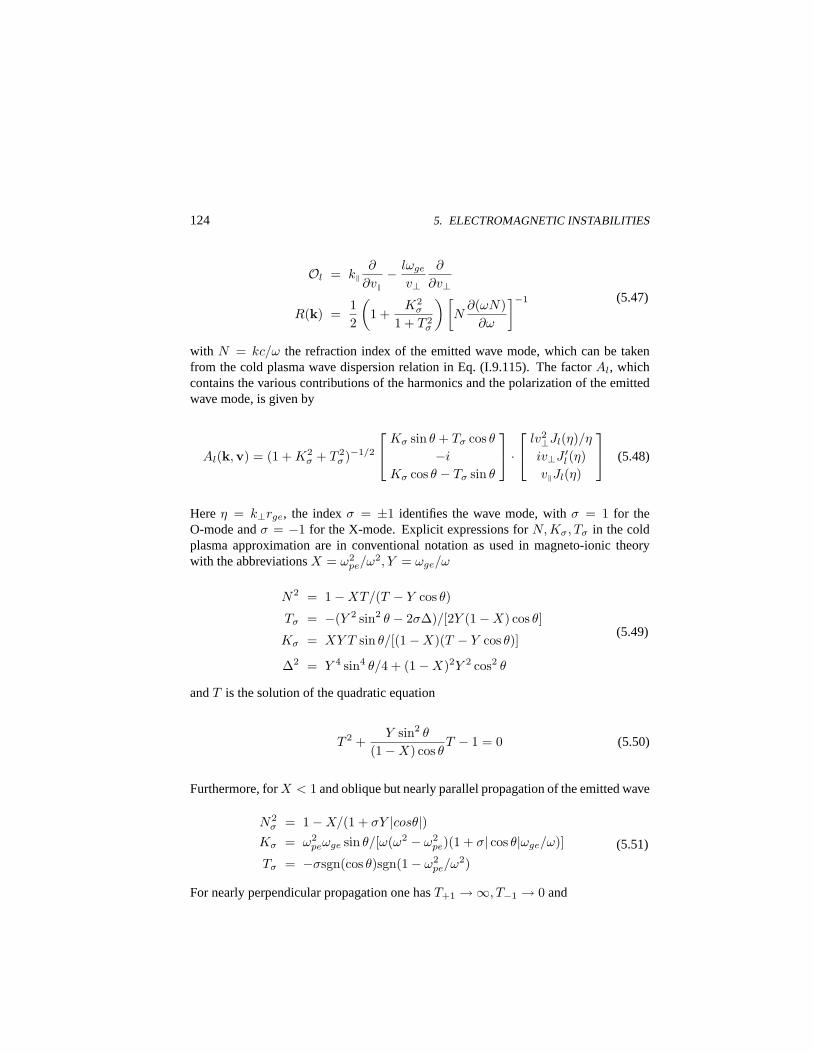
124 5. ELECTROMAGNETIC INSTABILITIES
Ol = k‖∂
∂v‖− lωge
v⊥
∂
∂v⊥
R(k) =12
(1 +
K2σ
1 + T 2σ
)[N
∂(ωN)∂ω
]−1 (5.47)
with N = kc/ω the refraction index of the emitted wave mode, which can be takenfrom the cold plasma wave dispersion relation in Eq. (I.9.115). The factorAl, whichcontains the various contributions of the harmonics and the polarization of the emittedwave mode, is given by
Al(k,v) = (1 + K2σ + T 2
σ )−1/2
Kσ sin θ + Tσ cos θ
−i
Kσ cos θ − Tσ sin θ
·
lv2⊥Jl(η)/η
iv⊥J ′l (η)v‖Jl(η)
(5.48)
Hereη = k⊥rge, the indexσ = ±1 identifies the wave mode, withσ = 1 for theO-mode andσ = −1 for the X-mode. Explicit expressions forN, Kσ, Tσ in the coldplasma approximation are in conventional notation as used in magneto-ionic theorywith the abbreviationsX = ω2
pe/ω2, Y = ωge/ω
N2 = 1−XT/(T − Y cos θ)
Tσ = −(Y 2 sin2 θ − 2σ∆)/[2Y (1−X) cos θ]
Kσ = XY T sin θ/[(1−X)(T − Y cos θ)]
∆2 = Y 4 sin4 θ/4 + (1−X)2Y 2 cos2 θ
(5.49)
andT is the solution of the quadratic equation
T 2 +Y sin2 θ
(1−X) cos θT − 1 = 0 (5.50)
Furthermore, forX < 1 and oblique but nearly parallel propagation of the emitted wave
N2σ = 1−X/(1 + σY |cosθ|)
Kσ = ω2peωge sin θ/[ω(ω2 − ω2
pe)(1 + σ| cos θ|ωge/ω)]
Tσ = −σsgn(cos θ)sgn(1− ω2pe/ω2)
(5.51)
For nearly perpendicular propagation one hasT+1 →∞, T−1 → 0 and
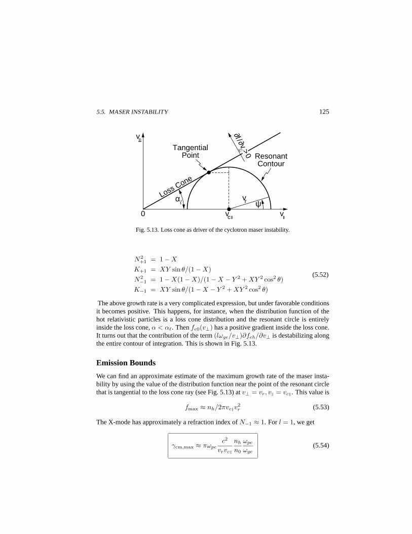
5.5. MASER INSTABILITY 125
vll
v⊥
vc ll
vr Loss Cone
Resonant Contour
Tangential Point
0
∂f /∂v⊥ >
0
α ψ
Fig. 5.13. Loss cone as driver of the cyclotron maser instability.
N2+1 = 1−X
K+1 = XY sin θ/(1−X)N2−1 = 1−X(1−X)/(1−X − Y 2 + XY 2 cos2 θ)
K−1 = XY sin θ/(1−X − Y 2 + XY 2 cos2 θ)
(5.52)
The above growth rate is a very complicated expression, but under favorable conditionsit becomes positive. This happens, for instance, when the distribution function of thehot relativistic particles is a loss cone distribution and the resonant circle is entirelyinside the loss cone,α < α`. Thenfe0(v⊥) has a positive gradient inside the loss cone.It turns out that the contribution of the term(lωge/v⊥)∂feh/∂v⊥ is destabilizing alongthe entire contour of integration. This is shown in Fig. 5.13.
Emission Bounds
We can find an approximate estimate of the maximum growth rate of the maser insta-bility by using the value of the distribution function near the point of the resonant circlethat is tangential to the loss cone ray (see Fig. 5.13) atv⊥ = vr, v‖ = vc‖. This value is
fmax ≈ nh/2πvc‖v2r (5.53)
The X-mode has approximately a refraction index ofN−1 ≈ 1. For l = 1, we get
γcm,max ≈ πωpec2
vrvc‖
nh
n0
ωpe
ωge(5.54)
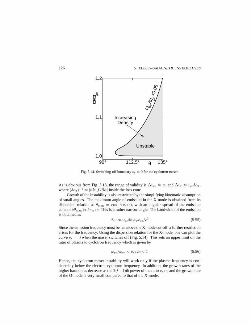
126 5. ELECTROMAGNETIC INSTABILITIES
Unstable
Increasing Density
ω pe/ω ge
=0.0
51.0
1.1
1.2
90° 135° θ
ω/ω
ge
112.5°
Fig. 5.14. Switching-off boundaryvr = 0 for the cyclotron maser.
As is obvious from Fig. 5.13, the range of validity is∆vc‖ ≈ vr and∆vr ≈ vc‖δα`,where(δα`)−1 ≈ |∂ ln f/∂α| inside the loss cone.
Growth of the instability is also restricted by the simplifying kinematic assumptionof small angles. The maximum angle of emission in the X-mode is obtained from itsdispersion relation asθmax = cos−1(vr/c), with an angular spread of the emissioncone ofδθmax ≈ δvc‖/c. This is a rather narrow angle. The bandwidth of the emissionis obtained as
∆ω ≈ ωgeδα`vrvc‖/c2 (5.55)
Since the emission frequency must be far above the X-mode cut-off, a further restrictionarises for the frequency. Using the dispersion relation for the X-mode, one can plot thecurvevr = 0 when the maser switches off (Fig. 5.14). This sets an upper limit on theratio of plasma to cyclotron frequency which is given by
ωpe/ωge < vr/2c < 1 (5.56)
Hence, the cyclotron maser instability will work only if the plasma frequency is con-siderably below the electron-cyclotron frequency. In addition, the growth rates of thehigher harmonics decrease as the2(l−1)th power of the ratiovr/c, and the growth rateof the O-mode is very small compared to that of the X-mode.
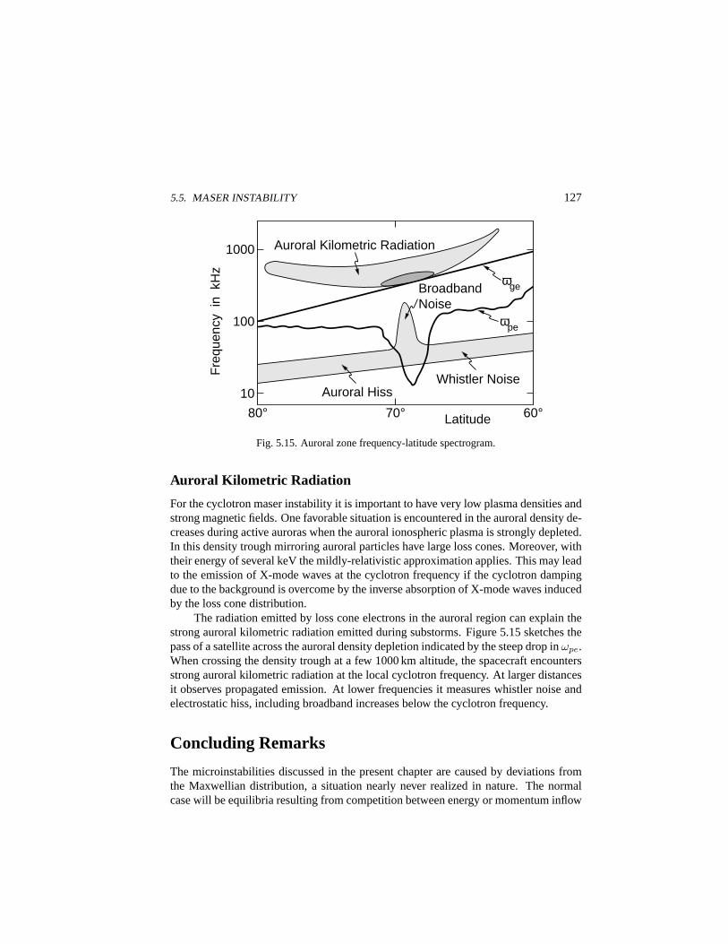
5.5. MASER INSTABILITY 127
10
100
1000 Auroral Kilometric Radiation
Broadband Noise
Auroral Hiss Whistler Noise
80° 70° 60° Latitude
Fre
quen
cy i
n k
Hz
ωge
ωpe
Fig. 5.15. Auroral zone frequency-latitude spectrogram.
Auroral Kilometric Radiation
For the cyclotron maser instability it is important to have very low plasma densities andstrong magnetic fields. One favorable situation is encountered in the auroral density de-creases during active auroras when the auroral ionospheric plasma is strongly depleted.In this density trough mirroring auroral particles have large loss cones. Moreover, withtheir energy of several keV the mildly-relativistic approximation applies. This may leadto the emission of X-mode waves at the cyclotron frequency if the cyclotron dampingdue to the background is overcome by the inverse absorption of X-mode waves inducedby the loss cone distribution.
The radiation emitted by loss cone electrons in the auroral region can explain thestrong auroral kilometric radiation emitted during substorms. Figure 5.15 sketches thepass of a satellite across the auroral density depletion indicated by the steep drop inωpe.When crossing the density trough at a few 1000 km altitude, the spacecraft encountersstrong auroral kilometric radiation at the local cyclotron frequency. At larger distancesit observes propagated emission. At lower frequencies it measures whistler noise andelectrostatic hiss, including broadband increases below the cyclotron frequency.
Concluding Remarks
The microinstabilities discussed in the present chapter are caused by deviations fromthe Maxwellian distribution, a situation nearly never realized in nature. The normalcase will be equilibria resulting from competition between energy or momentum inflow
128 5. ELECTROMAGNETIC INSTABILITIES
and dissipation in a system. A plasma is very sensitive to both of these because ofthe high mobility of its free or quasi-free particles. Instabilities of various kinds mayarise in these equilibria, saturate, and deform the distribution function, causing otherinstabilities to grow. Most of these processes are highly nonlinear, couple differentwave modes and affect the motion of the particles resonantly and non-resonantly.
Further Reading
The full drift kinetic electromagnetic tensor is derived in [4] and, in a particularly trans-parent form, in [1]. Microinstabilities, including a number of electromagnetic instabili-ties, are reviewed in [2], and [5]. Cyclotron waves and instabilities are found in [7] and[8]. The full theory of the whistler mode is contained in [6]. Numerical calculationsof many growth rates of electromagnetic instabilities are given in [1]. The cyclotronmaser mechanism is best reviewed in [5]. The auroral zone wave spectra are modeledafter Viking observations by Pottelette et al.,J. Geophys. Res. 97 (1992) 12029. Thedispersion curves and growth rates of the ion-cyclotron instability have been taken from[1].
[1] S. P. Gary,Theory of Space Plasma Microinstabilities(Cambridge University Press,Cambridge, 1993).
[2] A. Hasegawa,Plasma Instabilities and Nonlinear Effects(Springer Verlag, Heidel-berg, 1975).
[3] M. C. Kelley,The Earth’s Ionosphere(Academic Press, San Diego, 1989).
[4] N. A. Krall and A. W. Trivelpiece,Principles of Plasma Physics(McGraw-Hill,New York, 1971).
[5] D. B. Melrose,Instabilities in Space and Laboratory Plasmas, (Cambridge Univer-sity Press, Cambridge, 1991).
[6] S. Sazhin,Whistler-Mode Waves in a Hot Plasma(Cambridge University Press,Cambridge, 1993).
[7] T. H. Stix,Waves in Plasma(American Institute of Physics, New York, 1992).
[8] A. D. M. Walker, Plasma Waves in the Magnetosphere(Springer Verlag, Heidel-berg, 1993).
6. Drift Instabilities
The effect of spatial inhomogeneities in the plasma on the instabilities has so far beenneglected. However, for longer wavelengths, which are comparable to the natural scalesof the plasma,Ln = |∇ ln n|−1, LB = |∇ ln B|−1, andLT = |∇ ln T |−1, the changein the plasma parameters with space must be taken into account in the calculation of thewave properties. The result is a new type of waves calleddrift modeswhich are entirelydue to the presence of the plasma inhomogeneity..
Inclusion of inhomogeneity introduces a severe complication. In the fluid ap-proach it implies that the coefficients of the field variables become spatially dependent,and straight forward Fourier transformation of the basic equations is inhibited. In thesimplest case, when the inhomogeneity is only in one spatial direction, say onx, theplane wave ansatz is still possible in the two directionsy, z transverse to the directionof inhomogeneity. One then reduces the basic system of equations to an ordinary dif-ferential equation inx. For weak inhomogeneity one can take advantage of the furtherapproximation of expanding the inhomogeneities around a particular spatial position tofirst order inx. This approach is the local approximation and is used in the followingtheory.
6.1. Drift Waves
The fact that all plasmas are inevitably inhomogeneous and thus affected by gradientsin the plasma parameters implies that all plasmas are subject to drift wave propagationand drift instability. Accordingly, one calls the drift instability alsouniversal instability,meaning all kinds of drift instabilities without further specification. Clearly, drift insta-bilities can arise for all kinds of waves from electromagnetic Alfven and magnetosonicwaves up to ion-acoustic and plasma waves.
How the drift frequency arises can be understood from a dimensional inspectionof the linearized one-dimensional ion continuity equation in an inhomogeneous incom-pressible plasma
∂δni
∂t+ δvix
∂n0
∂x= 0 (6.1)
129
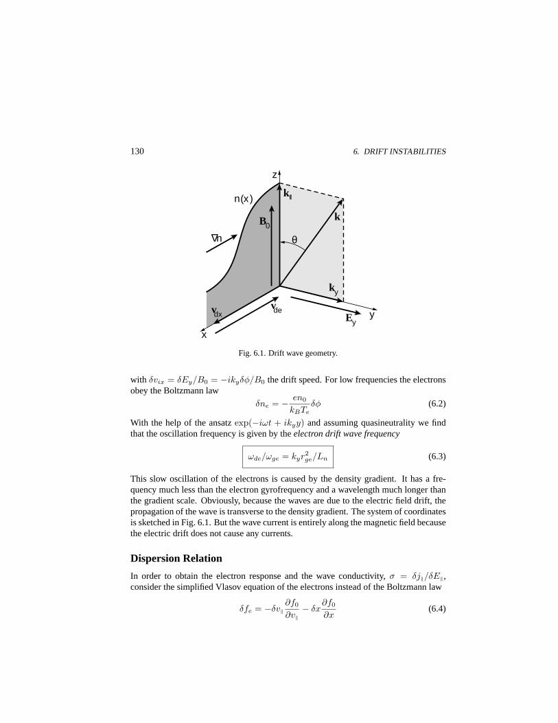
130 6. DRIFT INSTABILITIES
z
y vdx vde
B0
ky
k
θ
∆
n
n(x )
Ey
kll
x
Fig. 6.1. Drift wave geometry.
with δvix = δEy/B0 = −ikyδφ/B0 the drift speed. For low frequencies the electronsobey the Boltzmann law
δne = − en0
kBTeδφ (6.2)
With the help of the ansatzexp(−iωt + ikyy) and assuming quasineutrality we findthat the oscillation frequency is given by theelectron drift wave frequency
ωde/ωge = kyr2ge/Ln (6.3)
This slow oscillation of the electrons is caused by the density gradient. It has a fre-quency much less than the electron gyrofrequency and a wavelength much longer thanthe gradient scale. Obviously, because the waves are due to the electric field drift, thepropagation of the wave is transverse to the density gradient. The system of coordinatesis sketched in Fig. 6.1. But the wave current is entirely along the magnetic field becausethe electric drift does not cause any currents.
Dispersion Relation
In order to obtain the electron response and the wave conductivity,σ = δj‖/δE‖,consider the simplified Vlasov equation of the electrons instead of the Boltzmann law
δfe = −δv‖∂f0
∂v‖− δx
∂f0
∂x(6.4)

6.1. DRIFT WAVES 131
with the following expression for the linear excursion,δx, along the density gradient
δx = iδvx/(ω − k‖v‖) (6.5)
Furthermore, for electrostatic perturbations with vanishing∇× δE = 0 one has
k‖δEy = kyδE‖ (6.6)
and, sinceδvx = δEy/B0, the variation of the parallel electron distribution function is
δfe = −δE‖ie
me(ω − k‖v‖)
(∂
∂v‖+
ky
k‖ωge
∂
∂x
)f0 (6.7)
Using Plemelj’s formula (see Eq. (I.A.78) in the appendix of our companion book,Basic Space Plasma Physics) to replace the resonant denominator this becomes
δfe =πeδE‖
meδ(ω − k‖v‖)
(∂
∂v‖+
ky
k‖ωge
∂
∂x
)f0 (6.8)
One can express the parallel current by the integral
δj‖ = σδE‖ = −e
∞∫
−∞v‖dv‖δfe (6.9)
Since this is proportional to the disturbed electric field,δE‖, the wave conductivity is
σ(ω,k) = −πε0ω2pe
n0|k‖|ω
k‖
(∂
∂v‖+
ky
k‖ωge
∂
∂x
)f0
∣∣∣∣v‖=ω/k‖
(6.10)
Let the plasma density be inhomogeneous and otherwise use a Maxwellian undisturbeddistribution function, then the conductivity assumes the form
σe =π1/2ε0ω
2
k2‖λ
2D|k‖|vthe
(1− ωde
ω
)(6.11)
This expression, inserted into the dielectric function, given in Eq. (I.9.54) of the com-panion book, and repeated here
ε(ω,k) = I +iσ(ω,k)
ωε0(6.12)
yields a positive imaginary part ofε(ω,k) and may thus produce a drift instability.
132 6. DRIFT INSTABILITIES
Frequency and Growth Rate
An example of a drift wave instability due to a density gradient can be obtained bytaking a more precise fluid picture for the ions than used above in the dimensionalderivation of the drift frequency. If only density gradients exist,Ln is finite while allother scales go to infinity. The ion continuity equation then reads
∂δni/∂t +∇ · (n0δvi) = 0 (6.13)
where the density varies in space, and the oscillating ion velocity is given by the lin-earized and Fourier transformed ion drift velocity
δvi = δvE +ie
miω
(δE‖e‖ − ω2
ω2gi
δE⊥
)(6.14)
For simplicity the ions are assumed to be cold. Combining these equations and usingfor electrostatic wavesδE = −∇φ, one gets for a density gradient alongy
δni =en0
mi
(k2‖
ω2− k2
⊥ω2
gi
− k⊥Lnωωgi
)δφ (6.15)
The perturbed electron density is found from the above disturbed distribution as
δne = −(ik2‖/eω)σeδφ (6.16)
Since the plasma is quasineutral, combining the densities yields the dispersion relation
ε(ω,k) = 1 +k2⊥c2
ia
ω2gi
− k2‖c
2ia
ω2− ωde
ω+ i
(π
2
)1/2 ω
|k‖|vthe
(1− ωde
ω
)= 0 (6.17)
From here the real and imaginary parts of the frequency are obtained under the assump-tion thatk2
‖c2ia/ω2 < k2
⊥c2ia/ω2
gi ¿ 1 as
ωkd = ωde
(1− k2
⊥c2ia
ω2gi
)(6.18)
and
γkd =(π
2
)1/2 k2⊥c2
ia
ω2gi
ω2kd
|k‖|vthe(6.19)
This is the firstkinetic drift instabilitywe encounter. It is driven by the density gradientand exists only under the above condition on the parallel wavenumber. We note that forfinite plasmaβ this instability is quenched due to electron Landau damping.
6.2. KINETIC DRIFT WAVE THEORY 133
6.2. Kinetic Drift Wave Theory
If the influence of the plasma inhomogeneity on wave propagation and instability issmall, it will change the frequency only slightly. The natural drift wave frequency willthus fall into the low-frequency range so that the particle magnetic moments are con-served. Hence, the relevant kinetic equation to start from is either the gyrokinetic equa-tion (I.6.25) or the drift kinetic equation (I.6.27) from our companion book. Choosingthe latter
∂fd
∂t+
∂
∂xd· (vdfd) +
∂
∂v‖
(F‖m
fd
)= 0 (6.20)
with xd the guiding center coordinate and
vd⊥ = vE +F×BqB2
≈ vE +1
ωgB
dE⊥dt
vE =E×B
B2+
E‖ × δBB2
F = qE‖BB− µ∇B − 2kBT‖
R2c
Rc −mdvE
dt
(6.21)
Hereµ is the magnetic moment of the particles which is conserved during particle mo-tion in the low-frequency wave field, andRc = −(B/B·∇)B/B is the curvature radiusof the magnetic field. In addition we took into account the electric drift in a transversemagnetic field componentδB caused in presence of an electromagnetic wave.
Drift Kinetic Equation
In order to obtain the dispersion relation in a linearized theory, we take the followingseparation of the distribution function
fd(xd, µ, v‖, t) = f0d(xd, µ, v‖) + δfd(xd, µ, v‖, t) (6.22)
The undisturbed part does still depend on the spatial inhomogeneity of the plasma. Weneed to determine the plasma wave conductivity which enters the dielectric responsefunction. Hence, we need to calculate the disturbed plasma current. This current isgiven as the sum over all speciess in the guiding center approximation as
δj =∑
s
∫ [qsδvdsf0ds −∇×
(BB
µsδfds
)]dµdv‖ (6.23)
Note the normalization∫
fddµdv‖ = n0. The first term on the right-hand side accountsfor the drift current of the components, while the second term adds the diamagneticcurrent due to the gradients in the distribution function. For the latter we assume that
134 6. DRIFT INSTABILITIES
they are weak and that their characteristic scales are longer than the wavelength. Thusthe waves have wavelength short compared to the gradient scales.
We have the freedom to change the system of coordinates and to put the gradientalong they axis and let the wave vector,k = (k⊥, k‖), be in the(x, z) plane. Lookingfor electrostatic waves with electric field
δE = −∇δφ = −i(k⊥, 0, k‖)δφ (6.24)
the drift velocity in the inhomogeneous oscillating wave electric field is
δvd = −i
(k⊥B
ey +ω − k‖v‖
ωgBk⊥ex
)δφ (6.25)
The next step is to linearize the drift kinetic equation under the condition that the driftis caused in the inhomogeneous and oscillating wave field in the undisturbed inhomo-geneous plasma which yields
i(k‖v‖ − ω)δfd + δvdy∂fd0
∂y+ ik · δvd⊥fd0 +
q
mδE‖
∂fd0
∂v‖= 0 (6.26)
The undisturbed drifting distribution function,fd0, contains the inhomogeneity of theplasma, while the wave produces the polarization andE ×B drifts.
Dispersion Relation
Since the waves are electrostatic, we are interested only in the longitudinal part of thedielectric response function (5.2). By using the definition of the dielectric tensor in Eq.(6.12), this part can be expressed through the current. Then one can show that
k · σ · k = ik · δj/δφ (6.27)
where we used Ohm’s law for waves and the above representation of the wave electricfield through the electrostatic potential. Inserting into Eqs. (6.12) and (5.2) yields
εL(ω,k,x) = 1− k · δjε0ωk2δφ
(6.28)
Using an inhomogeneous but isotropic Maxwellian distribution as the undisturbed dis-tribution and evaluating the current, one gets the dielectric response function of driftwaves
εL(ω,k,x) = 1 +∑
s
ω2
ps
ω2gs
k2⊥
k2+
1k2λ2
Ds
[1−
(1− ωds
ω
)Z(ζs)
](6.29)
6.2. KINETIC DRIFT WAVE THEORY 135
The argument of the dispersion function isζs = ω/k‖vths and the drift wave frequencyωds which appears in the dispersion function is determined by
ωds = k · vds0 (6.30)
The zero-order drift velocity entering this expression is given by
vds0 = sgn(qs)vthsB× [(rrs∇) ln fds0] /B (6.31)
This drift frequencydepends on the inhomogeneity of the plasma which is containedin the spatial dependence of the zero-order distribution function. The drift velocity isthe diamagnetic drift velocity for the speciess. It is thus interesting that it is only thediamagnetic drift which gives rise to drift waves in a plasma. In other words, it is thevarious gradients which the pressure variation contributes that give rise to drift waves.
Electromagnetic Corrections
The simplified analysis presented here is based on two assumptions, the assumption ofsmall particle gyroradii and the electrostatic or longitudinal assumption. A more preciseand more sophisticated approach starts from the full Vlasov equation and expands thedistribution function up to first order iny with the expansion coefficientsL−1
n , L−1B ,
andL−1T , yielding for the longitudinal dielectric function
εL(ω,k,x) = 1 +∑
s
χLs(ω,k,x) (6.32)
with the susceptibilities,χLs, defined as
χLs(ω,k,x) =1
k2λ2Ds
1−
∞∑
l=−∞
[1−Os
(1 +
lω
ηsωgs
)]ω
ω − lωgsΛl(ηs)Z(ζs)
(6.33)where the differential operator,Os, is defined as
Os = sgn(qs)k⊥rgs cos θωgs
ω
[(rgs∇⊥) ln ns + (rgs∇⊥Ts)
∂
∂Ts
](6.34)
with θ the angle betweenk⊥ and thex axis. In many cases this operator can be approx-imated byOs ≈ ωds/ω.
The expression for the dielectric tensor becomes more complicated if one takesinto account electromagnetic interactions. In order to obtain it one follows the pro-cedure used to derive the magnetized dielectric tensor in Sec. 10.4 of our companionbook. The resulting dispersion relation becomes a function of frequency, wavenumber,and space coordinate
D(ω,k, x) = 0 (6.35)
136 6. DRIFT INSTABILITIES
Again, as has implicitly been done in the electrostatic case, this dispersion relation isevaluated in thelocal approximation, atx = 0, under the assumption that the gradientsare weak and the gradient length is longer than the wavelength and the gyroradius
rgs ¿ Ln, LB , LT (6.36)
a condition which is a prerequisite for the validity of the theory of adiabatic particlemotion. The most important change in the dispersion relation introduced by a densitygradient is that the resonant denominator in Eq. (1.35) is replaced according to
(k‖v‖ + lωgs − ω) → [k‖v‖ + (k⊥v2⊥/2Lnωgs) + lωgs − ω] (6.37)
This change of the resonance leads to the appearance of drift modes.
6.3. Drift Modes
Spatial inhomogeneities and the associated drift modes interact best with low-frequencywaves. Hence, the drift instability is most important for the excitation of ion-cyclotron,Alfv en, and lower-hybrid waves.
Drift-Cyclotron Instability
Cyclotron modes can become unstable in density gradients and excite thedrift-cyclotroninstability. From the electrostatic magnetized dispersion relation (1.35) one can derivethe following response function
ε(ω,k) = 1 +ω2
pe
ω2ge
+1
k2λ2Di
(1− ωdi
ω
) (1− ω√
2πk⊥rgi(ω − lωgi)
)= 0 (6.38)
Clearly, this equation has cyclotron harmonic solutions near the harmonics of the ioncyclotron frequencyω = lωgi. Instability is obtained under the condition that
rgi
Ln> 2l
(me
mi
)1/2(
1 +ω2
pe
ω2ge
)1/2
(6.39)
The right-hand side of the last condition reduces to the root of the mass ratio times2l whenever the plasma density is low. It is interesting to note that the condition forinstability sets an upper limit on the number of cyclotron harmonics. This propertydiffers from the current-, beam- or loss cone-driven cyclotron instabilities discussedabove, where the limit was set by the decrease of the growth rate. Here it appears as
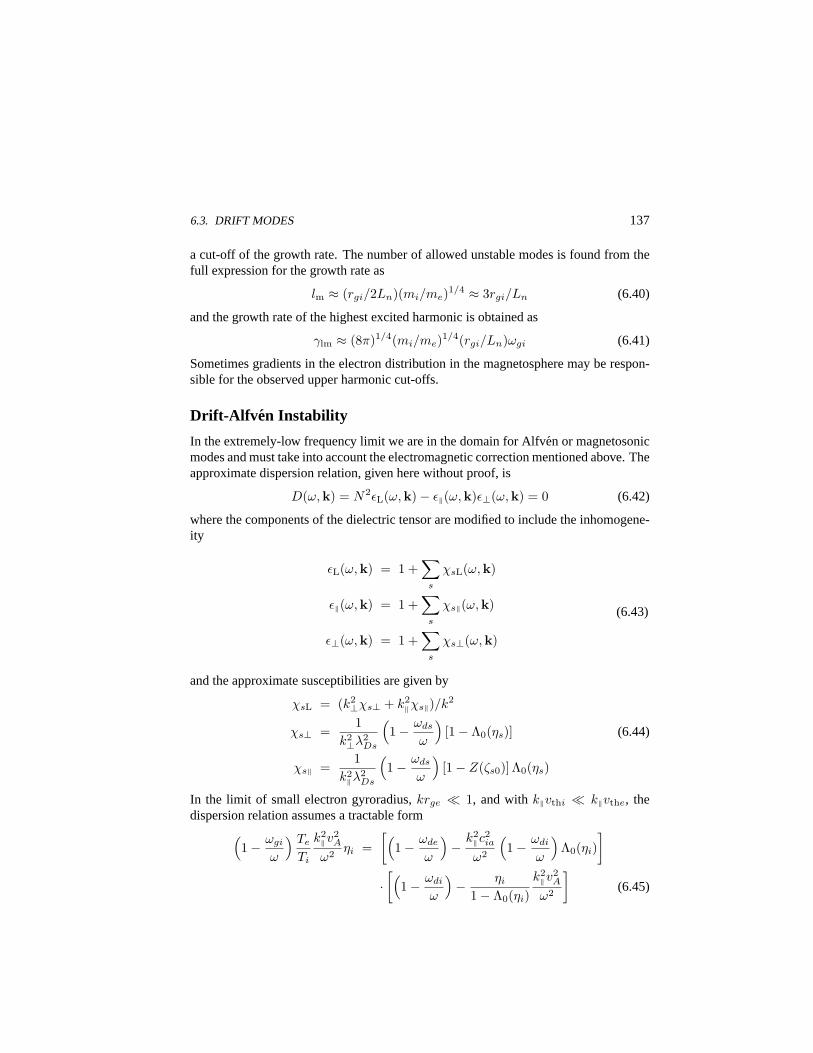
6.3. DRIFT MODES 137
a cut-off of the growth rate. The number of allowed unstable modes is found from thefull expression for the growth rate as
lm ≈ (rgi/2Ln)(mi/me)1/4 ≈ 3rgi/Ln (6.40)
and the growth rate of the highest excited harmonic is obtained as
γlm ≈ (8π)1/4(mi/me)1/4(rgi/Ln)ωgi (6.41)
Sometimes gradients in the electron distribution in the magnetosphere may be respon-sible for the observed upper harmonic cut-offs.
Drift-Alfv en Instability
In the extremely-low frequency limit we are in the domain for Alfven or magnetosonicmodes and must take into account the electromagnetic correction mentioned above. Theapproximate dispersion relation, given here without proof, is
D(ω,k) = N2εL(ω,k)− ε‖(ω,k)ε⊥(ω,k) = 0 (6.42)
where the components of the dielectric tensor are modified to include the inhomogene-ity
εL(ω,k) = 1 +∑
s
χsL(ω,k)
ε‖(ω,k) = 1 +∑
s
χs‖(ω,k)
ε⊥(ω,k) = 1 +∑
s
χs⊥(ω,k)
(6.43)
and the approximate susceptibilities are given by
χsL = (k2⊥χs⊥ + k2
‖χs‖)/k2
χs⊥ =1
k2⊥λ2
Ds
(1− ωds
ω
)[1− Λ0(ηs)] (6.44)
χs‖ =1
k2‖λ
2Ds
(1− ωds
ω
)[1− Z(ζs0)] Λ0(ηs)
In the limit of small electron gyroradius,krge ¿ 1, and withk‖vthi ¿ k‖vthe, thedispersion relation assumes a tractable form
(1− ωgi
ω
) Te
Ti
k2‖v
2A
ω2ηi =
[(1− ωde
ω
)− k2
‖c2ia
ω2
(1− ωdi
ω
)Λ0(ηi)
]
·[(
1− ωdi
ω
)− ηi
1− Λ0(ηi)k2‖v
2A
ω2
](6.45)
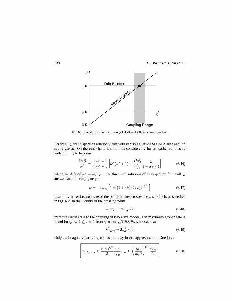
138 6. DRIFT INSTABILITIES
Coupling Range
Drift Branch
ω*
1.0
0.0
−0.5
k
Alfvén Branch
Fig. 6.2. Instability due to crossing of drift and Alfven wave branches.
For smallηi this dispersion relation yields with vanishing left-hand side Alfven and ionsound waves. On the other hand it simplifies considerably for an isothermal plasmawith Te = Ti to become
k2‖v
2A
ω2=
1ηi
ω∗ − 1ω∗ + 1
[ω∗(ω∗ + 1)− k2
‖v2A
ω2de
ηi
1− Λ0(ηi)
](6.46)
where we definedω∗ = ω/ωde. The three real solutions of this equation for smallηi
areωde, and the conjugate pair
ω = − 12ωde
[1± (
1 + 4k2‖v
2A/ω2
de
)1/2]
(6.47)
Instability arises because one of the pair branches crosses theωde branch, as sketchedin Fig. 6.2. In the vicinity of the crossing point
k‖vA =√
5ωde/4 (6.48)
instability arises due to the coupling of two wave modes. The maximum growth rate isfound forηe ¿ 1, ζ0e ¿ 1 from γ ∝ Im εL/(∂D/∂ω). It occurs at
k2‖max ≈ 2ω2
de/v2A (6.49)
Only the imaginary part ofεL comes into play in this approximation. One finds
γdA,max ≈ (πηi)1/2
3vA
vtheωde ≈
(me
miβ
)1/2vthi
Ln(6.50)
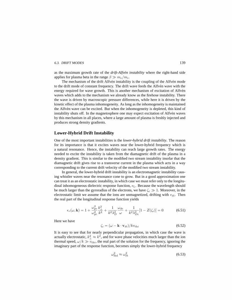
6.3. DRIFT MODES 139
as the maximum growth rate of thedrift-Alfven instabilitywhere the right-hand sideapplies for plasma beta in the rangeβ À me/mi.
The mechanism of the drift Alfven instability is the coupling of the Alfven modeto the drift mode of constant frequency. The drift wave feeds the Alfven wave with theenergy required for wave growth. This is another mechanism of excitation of Alfvenwaves which adds to the mechanism we already know as the firehose instability. Therethe wave is driven by macroscopic pressure differences, while here it is driven by thekinetic effect of the plasma inhomogeneity. As long as the inhomogeneity is maintainedthe Alfven wave can be excited. But when the inhomogeneity is depleted, this kind ofinstability shuts off. In the magnetosphere one may expect excitation of Alfven wavesby this mechanism in all places, where a large amount of plasma is freshly injected andproduces strong density gradients.
Lower-Hybrid Drift Instability
One of the most important instabilities is thelower-hybrid drift instability. The reasonfor its importance is that it excites waves near the lower-hybrid frequency which isa natural resonance. Hence, the instability can reach large growth rates. The energyneeded to excite the instability is taken from the diamagnetic drift of the plasma in adensity gradient. This is similar to the modified two stream instability insofar that thediamagnetic drift gives rise to a transverse current in the plasma which acts in a waycorresponding to the current drift velocity of the modified two stream instability.
In general, the lower-hybrid drift instability is an electromagnetic instability caus-ing whistler waves near the resonance cone to grow. But in a good approximation onecan treat it as an electrostatic instability, in which case we must refer only to the longitu-dinal inhomogeneous dielectric response function,εL. Because the wavelength shouldbe much larger than the gyroradius of the electrons, we haveζe À 1. Moreover, in theelectrostatic limit we assume that the ions are unmagnetized, drifting withvdi. Thenthe real part of the longitudinal response function yields
εr(ω,k) = 1 +ω2
pe
ω2ge
k2⊥
k2+
1k2λ2
D
ωde
ω+
1k2λ2
Di
[1− Z(ζi)] = 0 (6.51)
Here we haveζi = (ω − k · vdi)/kvthi (6.52)
It is easy to see that for nearly perpendicular propagation, in which case the wave isactually electrostatic,k2
⊥ ≈ k2, and for wave phase velocities much larger than the ionthermal speed,ω/k À vthi, the real part of the solution for the frequency, ignoring theimaginary part of the response function, becomes simply the lower-hybrid frequency
ω2lhd ≈ ω2
lh (6.53)
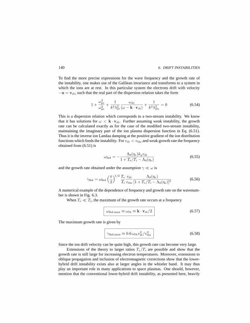
140 6. DRIFT INSTABILITIES
To find the more precise expressions for the wave frequency and the growth rate ofthe instability, one makes use of the Galilean invariance and transforms to a system inwhich the ions are at rest. In this particular system the electrons drift with velocity−u = vdi, such that the real part of the dispersion relation takes the form
1 +ω2
pe
ω2ge
+1
k2λ2D
ωde
(ω − k · vdi)+
1k2λ2
Di
= 0 (6.54)
This is a dispersion relation which corresponds to a two-stream instability. We knowthat it has solutions forω < k · vdi. Further assuming weak instability, the growthrate can be calculated exactly as for the case of the modified two-stream instability,maintaining the imaginary part of the ion plasma dispersion function in Eq. (6.51).Thus it is the inverse ion Landau damping at the positive gradient of the ion distributionfunctions which feeds the instability. Forvdi < vthi and weak growth rate the frequencyobtained from (6.51) is
ωlhd = − Λ0(ηe)kyvdi
1 + Te/Ti − Λ0(ηe)(6.55)
and the growth rate obtained under the assumptionγ ¿ ω is
γlhd = ωlhd
(π
2
)1/2 Te
Ti
vdi
vthi
Λ0(ηe)[1 + Te/Ti − Λ0(ηe)]2
(6.56)
A numerical example of the dependence of frequency and growth rate on the wavenum-ber is shown in Fig. 6.3.
WhenTe ¿ Ti, the maximum of the growth rate occurs at a frequency
ωlhd,max ≈ ωlh ≈ k · vdi/2 (6.57)
The maximum growth rate is given by
γlhd,max ≈ 0.6 ωlhv2di/v2
thi (6.58)
Since the ion drift velocity can be quite high, this growth rate can become very large.Extensions of the theory to larger ratiosTe/Ti are possible and show that the
growth rate is still large for increasing electron temperatures. Moreover, extensions tooblique propagation and inclusion of electromagnetic corrections show that the lower-hybrid drift instability exists also at larger angles in the whistler band. It may thusplay an important role in many applications to space plasmas. One should, however,mention that the conventional lower-hybrid drift instability, as presented here, heavily

6.3. DRIFT MODES 141
krgi
ω/ω
gi
2
γ/ω gi
4
6
8
10
0 10 20 30 40 50
0.5
1.0
1.5
2.0 ωlhd
γlhd
Fig. 6.3. Lower-hybrid drift instability forrgi/Ln = 0.5.
depends on plasmaβ. Whenβ increases toβ > 1, the instability is quenched. On theother hand, temperature gradients help to destabilize the instability. These are importantfacts which must be taken into account when applying the lower-hybrid drift instabilityto real space plasma conditions.
The lower-hybrid drift instability has been applied to low-frequency electrostaticwaves excited in the shock front region of the Earth’s bow shock, the density gradientregion at the magnetopause and in the low latitude boundary layer, the density gradientregion in the Earth’s magnetotail plasma sheet, and the density gradients in the upperionosphere. Excitation of lower-hybrid drift waves at the bow shock is probably sup-pressed by the high beta of the oncoming solar wind. More important is the excitationof lower-hybrid drift waves in the gradients at the magnetopause, both the transitionregion and the low latitude boundary layer. Relatively high wave intensities have beenreported here close to the lower-hybrid frequency. Lower-hybrid waves may add totransport of cold plasma across the magnetopause if the wave intensities are high.
Lower-hybrid waves can be excited in the tail plasma sheet as long as one staysoutside of the neutral sheet current layer proper. The increase in the measured electricwave spectra toward low frequencies in Fig. 4.17 is an indication of the presence oflower-hybrid waves in the tail (for plasma sheet conditions the lower-hybrid frequencyis close to 10 Hz). In the ionosphere, in spite of the steep density gradients appearing inthe E- and F-layers, the lower-hybrid drift instability is stabilized by the presence of fre-quent collisions. Nevertheless, it can evolve under special circumstances at occasionalvery steep gradients.
142 6. DRIFT INSTABILITIES
Concluding Remarks
Drift instabilities are sometimes also calleduniversal instabilitiesa term indicating thatdrift instabilities are the most general linear instabilities which appear in almost everyplace and at all occasions. The reason is that plasmas are always inhomogeneous at leaston the microscopic scales. One may therefore be sure that drift instabilities will be metunder all realistic conditions. Their importance cannot be overestimated. Neverthelesswe have treated them only in passing because their linear treatment is standard.
In space and astrophysical plasmas drift instabilities naturally play an importantrole. However, though in space plasmas they have been detected in situ and are wellknown to generate particle loss, excite waves and lead to anomalous transport, heatingand energy dissipation, their importance has not yet been recognized for astrophysicalplasmas. In particular, the lower hybrid drift instability, which we have treated in length,is very important in providing anomalous resistivities, transport, and heat conduction.Some of these questions will be treated in the last chapter of this volume.
Further Reading
The full drift kinetic electromagnetic tensor is derived in [2], in [3], and in a particularlytransparent form in [1]. A short but informative article on instabilities in inhomoge-neous plasmas is found in [4].
[1] S. P. Gary,Theory of Space Plasma Microinstabilities(Cambridge University Press,Cambridge, 1993).
[2] N. A. Krall and A. W. Trivelpiece,Principles of Plasma Physics(McGraw-Hill,New York, 1971).
[3] A. B. Mikhailovskii, Theory of Plasma Instabilities II(Consultants Bureau, NewYork, 1976).
[4] A. B. Mikhailovskii, in Handbook of Plasma Physics, Vol. 1, eds. A. A. Galeev andR. N. Sudan (North-Holland Publ. Co., Amsterdam, 1983), p. 586
7. Reconnection
The magnetohydrodynamic instabilities discussed in Chap. 3 are ideal instabilities.They lead to bending and deformation of magnetic flux tubes, but the frozen-in con-dition remains valid. This condition breaks down when the plasma becomes non-ideal.Whenever this happens, the magnetic field starts diffusing across the plasma, and mag-netic flux can be exchanged between different plasmas in mutual contact. The processof magnetic flux exchange is a diffusive process with magnetic diffusivity resultingfrom either collisions or being the consequence of nonlinear interactions of the kindreviewed in Chap. 12. Any such diffusion process implies that the magnetic field lines,which in an ideal plasma can be considered as unbreakable strings, are re-ordered suchthat the field line configuration after re-ordering looks different from the initial one.
Physically the magnetic flux is rearranged during diffusion, a process which usu-ally is slow. However, in some model cases this kind of re-ordering can become com-parably fast when the diffusion process is restricted to a region of small spatial extent.This is the important case when one speaks ofmagnetic reconnection. Magnetic re-connection or merging plays a key role in the processes at the magnetopause, in themagnetotail, in solar active regions, and in a number of astrophysical applications likeaccretion disks. It has experienced enormous attention in the space plasma communityduring the last forty years. Both, remote and in situ observations of magnetic diffusionprocesses in space have revealed that re-ordering of magnetic fields may proceed atvery high speeds when restricted to narrow spatial regions.
It must be emphasized that from the physical point of view there is nothing par-ticular about reconnection insofar as any process which causes violation of the idealconditions in a plasma and thus leads to collisional effects, always results in diffusionof magnetic fields and thus reconnection and rearranged magnetic field topology. Thereal question is how and where such diffusivities are generated in an otherwise idealor collisionless plasma. But once they exist, it is quite natural that oppositely directedfield components will cancel each other and cause reconnection. In the following wereview the currently accepted and competing reconnection models for both collisionaland collisionless plasmas. Since in the collisional case the diffusivity is natural and itsorigin must not be explained, we start with the collisional reconnection models beforediscussing some versions of collisionless reconnection.
143

144 7. RECONNECTION
7.1. Reconnection Rates
Consider two mutually approaching ideal magnetohydrodynamic flows containing op-positely directed magnetic fields until they meet in a plane atx = 0, as shown in Fig.7.1. In ideal magnetohydrodynamics the frozen-in condition requires that each flowelement is fixed to its particular field line. Hence, when the flows meet they will beunable to mix and pressure balance will slow them down and force them to rest. Butif the magnetic fields in the two flows are oppositely directed and of the same strength,they may annihilate each other at the plane of contact, allowing the plasmas to mix.
Magnetic Diffusion
Mixing and annihilation is permitted only when the plasma is non-ideal, because onlythen the magnetic field can diffuse across the flow and annihilate. This is described bythe general induction equation (I.5.2) in our companion book
∂B∂t
= ∇× (v ×B) +1
µ0σ∇2B (7.1)
whereσ is the constant electrical conductivity. The diffusion time of the magnetic fieldis given in Eq. (I.5.6) of our companion book
τd = L2σµ0 (7.2)
whereL is the global length scale of the change inB, and the diffusion velocity is
vd = L/τd = 1/Lσµ0 (7.3)
z
x
−vx +vx
+Bz
−Bz
Fig. 7.1. Counterstreaming flows leading to reconnection.
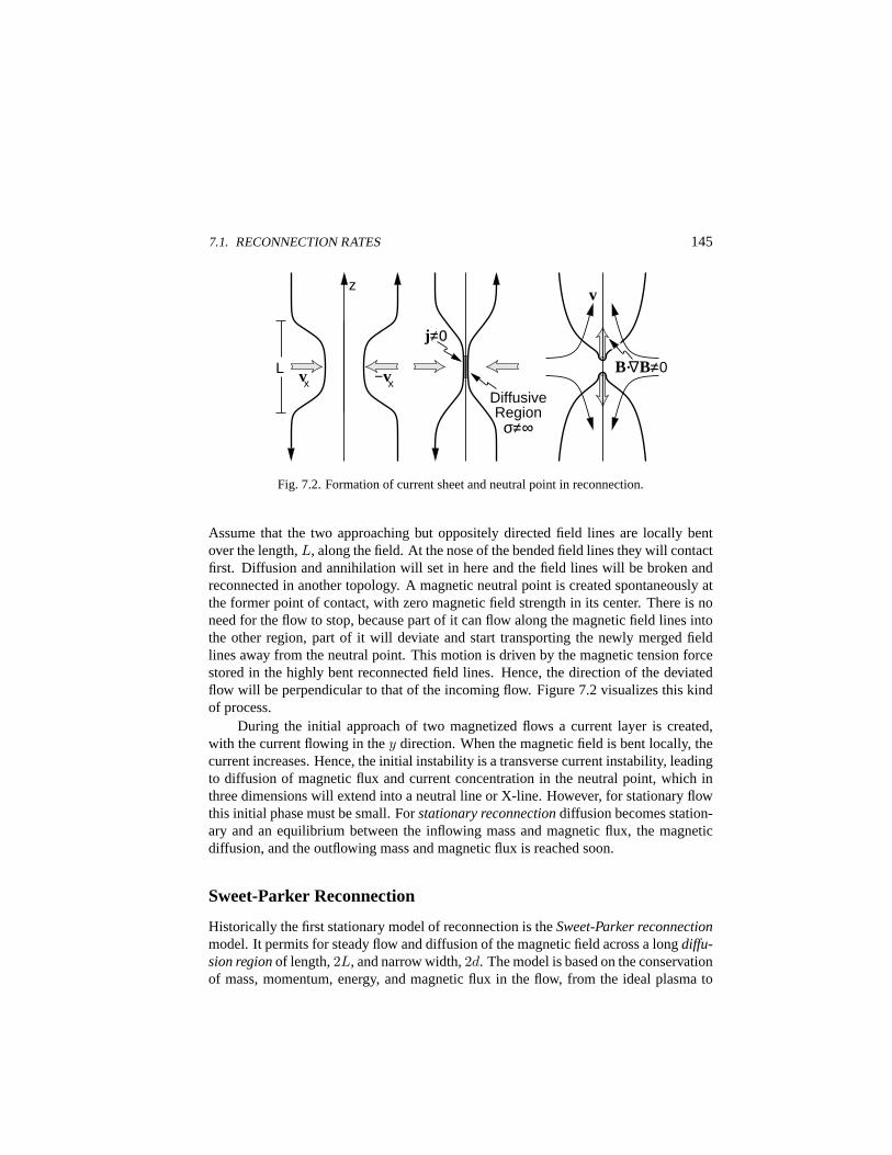
7.1. RECONNECTION RATES 145
j≠0
Diffusive Region
σ≠∞
L vx −vx
z v
B· B≠0
∆
Fig. 7.2. Formation of current sheet and neutral point in reconnection.
Assume that the two approaching but oppositely directed field lines are locally bentover the length,L, along the field. At the nose of the bended field lines they will contactfirst. Diffusion and annihilation will set in here and the field lines will be broken andreconnected in another topology. A magnetic neutral point is created spontaneously atthe former point of contact, with zero magnetic field strength in its center. There is noneed for the flow to stop, because part of it can flow along the magnetic field lines intothe other region, part of it will deviate and start transporting the newly merged fieldlines away from the neutral point. This motion is driven by the magnetic tension forcestored in the highly bent reconnected field lines. Hence, the direction of the deviatedflow will be perpendicular to that of the incoming flow. Figure 7.2 visualizes this kindof process.
During the initial approach of two magnetized flows a current layer is created,with the current flowing in they direction. When the magnetic field is bent locally, thecurrent increases. Hence, the initial instability is a transverse current instability, leadingto diffusion of magnetic flux and current concentration in the neutral point, which inthree dimensions will extend into a neutral line or X-line. However, for stationary flowthis initial phase must be small. Forstationary reconnectiondiffusion becomes station-ary and an equilibrium between the inflowing mass and magnetic flux, the magneticdiffusion, and the outflowing mass and magnetic flux is reached soon.
Sweet-Parker Reconnection
Historically the first stationary model of reconnection is theSweet-Parker reconnectionmodel. It permits for steady flow and diffusion of the magnetic field across a longdiffu-sion regionof length,2L, and narrow width,2d. The model is based on the conservationof mass, momentum, energy, and magnetic flux in the flow, from the ideal plasma to

146 7. RECONNECTION
both sides of the diffusion region into and out of the diffusion region. From Ampereslaw the current flowing in the diffusion region is given by
jdy ≈ B0z/µ0d (7.4)
The Lorentz force entering the momentum conservation equation consists of two terms,the magnetic pressure and the magnetic stress resulting from the bending of the mag-netic field lines during magnetic merging and subsequent reconnection. The pressureforce term is compensated due to general pressure balance, provided the boundary is atrest. The magnetic stresses accelerate the plasma into thez direction over the lengthL
(jdy ×Bdx) · ez ≈ jdyBdx = B0zBdx/µ0d (7.5)
In the stationary case, this force balances the nonlinear velocity term in the momentumequation
nmi(v · ∇)vdz ≈ nmiv2dz/L ≈ B0zBdx/µ0d (7.6)
Since the magnetic field is divergence-free, we have
B0z/L ≈ Bdx/d (7.7)
so that the equation for the outflow velocity becomes
v2dz ≈ B2
0z/µ0nmi = v2A0 (7.8)
which is the Alfven speed in the inflowing plasma. For a plasma moving into the dif-fusion region with inflow speedv0x we can estimate the efficiency of the reconnectionprocess by defining areconnection rate, R = v0x/vdz = MA0, which is equal tothe incident Mach number. Under stationary conditions the plasma leaves the neutralpoint region with the Alfven speed of the inflowing plasma. Hence, the reconnectionproceeds via a large-amplitude Alfven wave. Actually, it is a rotational discontinuity,where the normal component of the magnetic field is produced by the reconnectionprocess.
The magnetic field is incompressible and carried into and out of the diffusion re-gion at the speed of the flow. Hence, we have in analogy to Eq. (7.3)
v0x = 1/dσµ0 (7.9)
with 2d the width of the diffusion region. Conservation of mass requires that the rate ofmass inflow equals that of the outflow. Because of the incompressibility of the medium
v0xL ≈ vA0d (7.10)
Now we can eliminate the width of the diffusion layer,d, obtaining
v20x ≈ vA0/Lσµ0 (7.11)
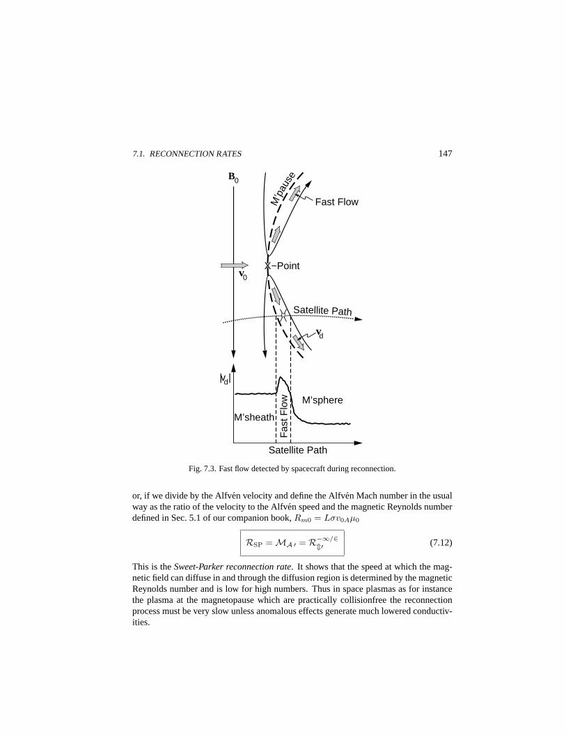
7.1. RECONNECTION RATES 147
X
Satellite Path
M’p
ause
−Point
B0
v0
M’sphere
vd
Fast Flow
Fas
tFlo
w
|vd|
M’sheath
Satellite Path
Fig. 7.3. Fast flow detected by spacecraft during reconnection.
or, if we divide by the Alfven velocity and define the Alfven Mach number in the usualway as the ratio of the velocity to the Alfven speed and the magnetic Reynolds numberdefined in Sec. 5.1 of our companion book,Rm0 = Lσv0Aµ0
RSP = MA ′ = R−∞/∈m′ (7.12)
This is theSweet-Parker reconnection rate. It shows that the speed at which the mag-netic field can diffuse in and through the diffusion region is determined by the magneticReynolds number and is low for high numbers. Thus in space plasmas as for instancethe plasma at the magnetopause which are practically collisionfree the reconnectionprocess must be very slow unless anomalous effects generate much lowered conductiv-ities.
148 7. RECONNECTION
Reconnection implies that the inflowing magnetic energy density is much largerthan the inflowing kinetic energy
µ0nmiv20x/B2
0z = M2A0 ¿ 1 (7.13)
Concerning the outflow, we recognize that magnetic flux must be conserved
v0xB0z = vdzBdx (7.14)
Forming the ratio of the outflowing kinetic power,nmiv3dzd/2, to the inflowing mag-
netic power,v0xB20zL/µ0, we get
µ0nmiv3dzd
2 v0xB20zL
=v3
dz
2v3A0
=12
(7.15)
Half the inflowing magnetic energy is converted into flow energy and thus transformedinto acceleration. Hence, reconnection at neutral points generates high-speed flows es-caping from the neutral point and serves as a plasma acceleration mechanism. Thesehigh-speed flows have actually been detected by spacecraft during high magnetic shearmagnetopause crossings, thus indicating that the magnetopause can behave as a rota-tional discontinuity undergoing magnetic merging. From the direction of the flow onecan determine the position of the neutral point relative to the spacecraft (see Fig. 7.3).
Petschek Reconnection
Sweet-Parker reconnection requires long current sheets and is a rather slow process.When the finite conductivity is restricted to a more localized region, the reconnectionprocess becomes faster becauseL is shorter. This mechanism does, however, requiremore complicated processes to work at the magnetopause near the reconnection site.The outer region has no current flow and, since reconnection proceeds only in a smalldiffusion region around the neutral point, not all plasma can cross the diffusion region.Most of the plasma must turn around before reaching the interface between the twocounterstreaming flows. Because this change in flow direction and speed will be abrupt,it must occur at a shock. Since the magnetic field lines are refracted toward the shocknormal, the shocks involved areslow mode shocks(cf. Fig. 8.11 in our companion bookand Fig. 7.4 in this volume). Here 3/5 of the inflowing magnetic energy are convertedinto kinetic energy behind the shock, the remaining 2/5 are used to heat the plasma.
Although there is no reconnection at the shocks, a normal component,Bn, exists.The slow shocks are large-amplitude slow magnetosonic waves, which in a hot plasmatravel with the Alfven speed based on its normal field
v2ss = B2
n/nmiµ0 (7.16)

7.1. RECONNECTION RATES 149
−B0
+B0
+Bn x
z −Bn
∆
2 B=
0
∆
2 B=
0
L
−Bn
Slow Shocks
Pat
h o
f In
tegr
atio
n
+Bn
Fig. 7.4. Mechanism of Petschek Reconnection.
Figure 7.4 shows the idealized geometry of the Petschek model with the narrow andshort diffusion region of length along z and the four slow shocks connected to it.These shocks extend into the current-free environment, where∇2B = 0. The shockschange the direction of the magnetic field by 90, as is required for reconnection. Thesefields are the reconnected fields which leave, as in the Sweet-Parker model, from thediffusion region and are driven by magnetic stresses.
The field change at the shock is a disturbance of the initial external field,B0, inthe outer region. This disturbance can be calculated assuming that each element of theshock causes a small magnetic disturbance,δB = b/z, which decays with distanceof the element from the diffusion region along the shock surface,z. The flux causedby it is the product of the disturbance field and the surface element in one dimension,πz, yieldingπzb/z = bπ. But because the element has the lengthdz along the shock,the flux is also equal to2Bndz and thusb = (2Bn/π)dz. Integrating along the shocklength,L, over all contributions of the elements excluding the diffusion region of length,`, where no shocks exist, gives
2Bn
π
(∫ −`/2
−L/2
dz
z−
∫ L/2
`/2
dz
z
)= −4Bn
πln
(L
`
)(7.17)
This field must be added to the external field at large distances. The result is
B0z = B0
[1− 4MA0
πln
(L
`
)](7.18)
150 7. RECONNECTION
where Eq. (7.16) and the definition of the Mach number have been used. The externalMach number is small. Therefore the total external field is nearly the field at largedistances in this case. If we write the ratio of the length of the diffusion region to thelateral scale as
`/L = 1/(Rm0MA0) (7.19)
it is obvious that the dimension,`, of the diffusion region will decrease if either themagnetic Reynolds number or the reconnection rate increase. Hence, high reconnectionrates require a narrow diffusion region and the process stops when their lateral extentbecomes too short. As Petschek suggested, the maximum reconnection rate will beachieved forB0z = B0/2. This yields, instead of the Sweet-Parker reconnection rategiven in Eq. (7.12), in the limit of large Reynolds numbers the much faster maximumPetschek reconnection rate
RP ≈ π/∀ lnRm′ (7.20)
It depends only logarithmically on the Reynolds number and varies much less withconductivity. Petschek reconnection is therefore a very efficient mechanism to mergemagnetic fields and to provide magnetic diffusion through narrow diffusion regions.
Because the conductivities in space plasmas are so high, Sweet-Parker reconnec-tion is usually a very inefficient process which will not lead to violent mixing of mag-netic fields and the related energy releases. Processes which locally decrease the con-ductivity will enhance reconnection. But Petschek reconnection, whenever it occurs,will always be much faster providing fast dissipation and effective mixing as well asviolent acceleration of plasma from the reconnection region. However, it is at presentnot clear that Petschek reconnection can evolve in natural systems.
7.2. Steady Collisionless Reconnection
The reconnection rates given in the previous section all refer to the collisional regimewith at least a small resistivity. In space plasmas such resistivities do not exist a priori.Hence, the magnetohydrodynamic approach becomes invalid, and one should switch toa steady kinetic approach where particle dynamics initiates reconnection. In the nextsections we will consider an instability, thetearing mode, which may work in both theresistive and collisionless regimes. Here we briefly discuss the possibility of a steadycollisionless state.
Linear Regime
Consider a two-dimensional configuration with all quantities independent ofy. Thisconfiguration is shown schematically in Fig. 7.5. Then the magnetic field can be repre-sented asB = −ey × ∇A(x, z), whereA is the only surviving vector potential com-
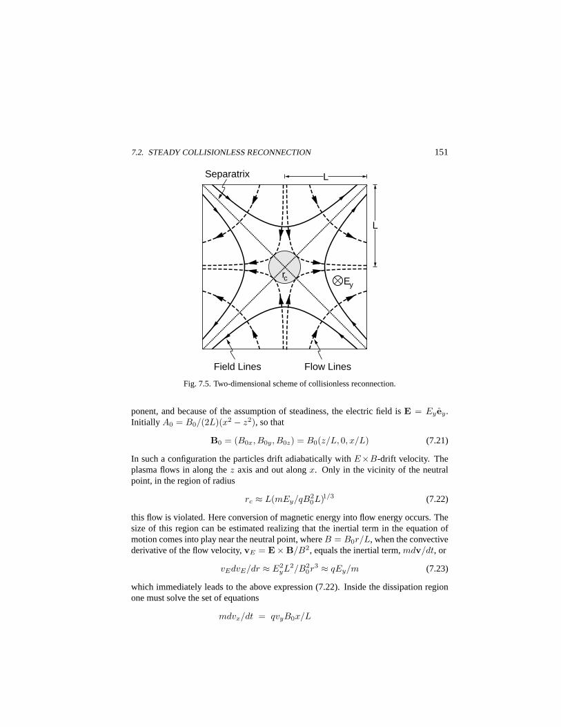
7.2. STEADY COLLISIONLESS RECONNECTION 151
Flow Lines Field Lines
L
L
Ey rc
Separatrix
Fig. 7.5. Two-dimensional scheme of collisionless reconnection.
ponent, and because of the assumption of steadiness, the electric field isE = Eyey.Initially A0 = B0/(2L)(x2 − z2), so that
B0 = (B0x, B0y, B0z) = B0(z/L, 0, x/L) (7.21)
In such a configuration the particles drift adiabatically withE×B-drift velocity. Theplasma flows in along thez axis and out alongx. Only in the vicinity of the neutralpoint, in the region of radius
rc ≈ L(mEy/qB20L)1/3 (7.22)
this flow is violated. Here conversion of magnetic energy into flow energy occurs. Thesize of this region can be estimated realizing that the inertial term in the equation ofmotion comes into play near the neutral point, whereB = B0r/L, when the convectivederivative of the flow velocity,vE = E×B/B2, equals the inertial term,mdv/dt, or
vEdvE/dr ≈ E2yL2/B2
0r3 ≈ qEy/m (7.23)
which immediately leads to the above expression (7.22). Inside the dissipation regionone must solve the set of equations
mdvx/dt = qvyB0x/L
152 7. RECONNECTION
mdvy/dt = qEy + q(vzBx − vxBz) (7.24)
mdvz/dt = −qvyB0z/L
A particle entering the X-point is accelerated by the electric field in they direction andreceives a speedvy(t) ≈ qEyt/m, while theBz component wants to eject the particlefrom the X-line in thex direction, andBx leads to an oscillation alongz, so that
d2x/dt2 = tx/t3c
d2z/dt2 = −ω2b (t)z
(7.25)
where the critical acceleration time inx and the oscillation period inz are given by
tc = (m2L/q2B0Ey)1/3
ωb(t) = (q2B0Eyt/m2L)1/2 (7.26)
Hence, the ejection from the X-line proceeds exponentially asexp(t/tc)3/2, and theparticle reachesrc at timetc when the velocity becomesvc ≈ rc/tc ≈ (qE2
yL/mB)1/3.The gain in particle velocity is in thevy component and is of course of the order ofvc.It is thus transformed into the transverse energy of the particle drifting away from theX-line. The energy turns out to be proportional tom1/3 such that the main dissipationis due to ions rather than electrons. Moreover, the net electric current is carried bythe ions, because it is basically a polarization current,I ≈ enivcr
2c . It is therefore
sufficient to consider the ion motion. In other words, the collisionless reconnection inthis approximation is driven by ion inertia.
Outside the dissipation region ion dynamics is simple electric drift with stream-lines
dx/vEx = dz/vEz (7.27)
which are hyperbolic withxz = const. The ion flux entering the dissipation region isbounded by the streamline withxc ≈ zc ≈ rc and, for steady flow,
n0xLvEz(L) = nixcvEz(rc) (7.28)
wherene is the undisturbed electron background density, and the indexL as well as thedependence onL indicate that the corresponding quantities must be taken at distanceL(or at infinity). Taking into account the electric field drift expressions, one finds for ionnumber and current densities
ni ≈ n0(rc/L)2 ≈ n0(miEy/eLB20)2/3
j ≈ enivc ≈ en0(Ey/B0)(miEy/eLB20)1/3 (7.29)

7.2. STEADY COLLISIONLESS RECONNECTION 153
Thus the total magnetic energy dissipation is proportional to the third power of theelectric field,QB = EyI ∝ E3
y .When the magnetic field generated by the electric current becomes comparable to
the initial field,B0, this linear approximation will break down. This takes place at afield strengthδB ∝ µ0jr/2. Replacing the current density and radius in this expressionand using the external Mach number,MA0 = v0/vA0, with v0 = Ey/B0 gives thefollowing limit for the linear regime
MA0 ≤ Mc = R−1/4m0 (7.30)
where the Reynolds number has been defined as the ratio of the total length to theexternal ion inertial length,Rm0 = (Lωpi/c)1/2. This indicates that the reconnectionis determined by the ion inertia. The collisionless Reynolds number is very large forlargeL and small inertial lengths. But the Reynolds number enters at the fourth root ofthis ratio. For larger reconnection rates one must extend the calculation to the nonlinearregime.
We now simplify to the incompressible case outside the reconnection region faraway from the X-line. Then the external ion density is equal ton0, and
j ≈ en0v0 ≈ en0(eLE2y/miB0)1/3 (7.31)
The linear approximation holds under the restriction on the electric field
Ey ≤ Eyc = miv2A0c/eL2ωpi (7.32)
which may be written asMA0 ≤ M∗ ≈ R−1m0. This condition is more restrictive than
Eq. (7.30) and readily violated. Then reconnection enters the nonlinear regime.
Nonlinear Regime
We now sketch the nonlinear estimates for the assumed large reconnection rates. Theelectric field isEy > Eyc. Let us use dimensionless quantities with the electric fieldnormalized toEyc, length toc/ωpi, magnetic field toB0c/Lωpi, and time toL/vA0.This yields the normalized vector potentialA0 = (x2 − z2)/2. The geometry is shownin Fig. 7.6. It is an elongated reconnection site of length2L and width2d for the nor-malized electric fieldEy À 1, far above the critical field,Eyc. ThendBx/dz ≈ j forthe normalized magnetic field and current in the reconnection site, under the assumptionthat we can take the current as constant. From the condition∇ ·B = 0 we obtain
Bz(x) ≈ jd
π
L+x∫
L−x
dξ
ξ≈ 2jd
π
x
L(7.33)
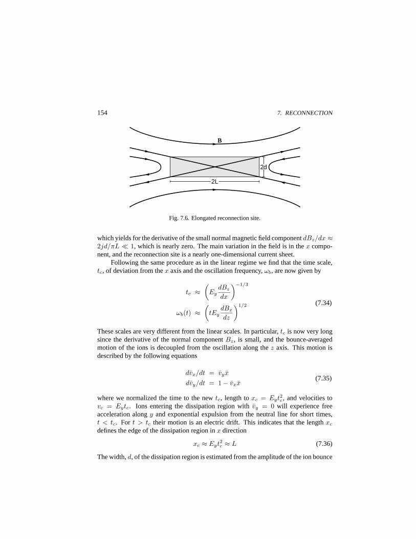
154 7. RECONNECTION
B
2L
2d
Fig. 7.6. Elongated reconnection site.
which yields for the derivative of the small normal magnetic field componentdBz/dx ≈2jd/πL ¿ 1, which is nearly zero. The main variation in the field is in thex compo-nent, and the reconnection site is a nearly one-dimensional current sheet.
Following the same procedure as in the linear regime we find that the time scale,tc, of deviation from thex axis and the oscillation frequency,ωb, are now given by
tc ≈(
EydBz
dx
)−1/3
ωb(t) ≈(
tEydBx
dz
)1/2 (7.34)
These scales are very different from the linear scales. In particular,tc is now very longsince the derivative of the normal componentBz, is small, and the bounce-averagedmotion of the ions is decoupled from the oscillation along thez axis. This motion isdescribed by the following equations
dvx/dt = vyx
dvy/dt = 1− vxx(7.35)
where we normalized the time to the newtc, length toxc = Eyt2c , and velocities tovc = Eytc. Ions entering the dissipation region withvy = 0 will experience freeacceleration alongy and exponential expulsion from the neutral line for short times,t < tc. For t > tc their motion is an electric drift. This indicates that the lengthxc
defines the edge of the dissipation region inx direction
xc ≈ Eyt2c ≈ L (7.36)
The width,d, of the dissipation region is estimated from the amplitude of the ion bounce
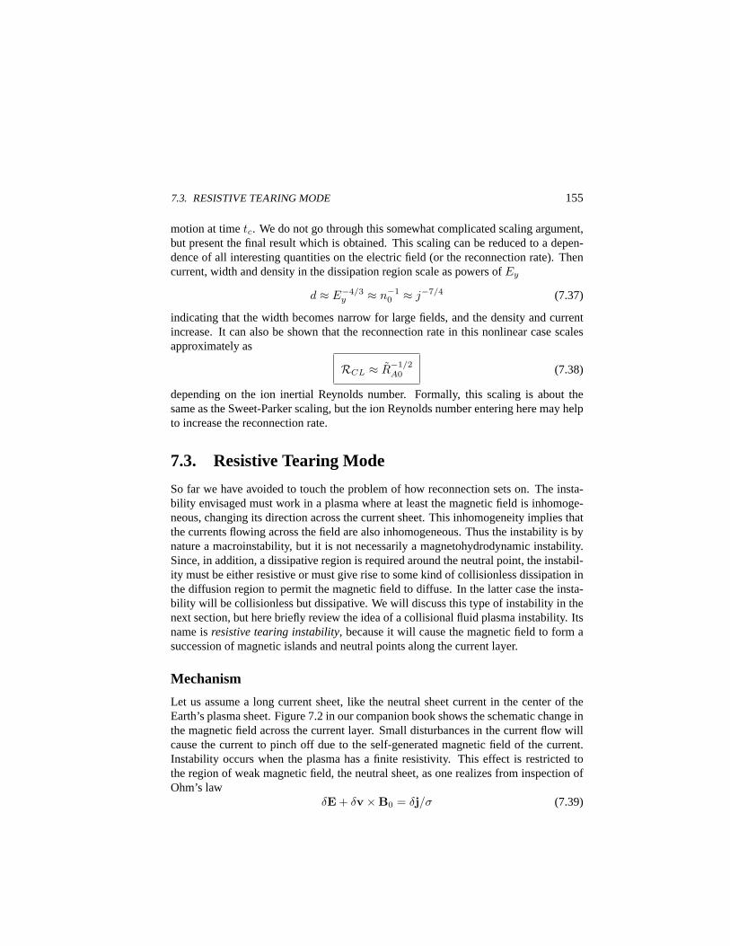
7.3. RESISTIVE TEARING MODE 155
motion at timetc. We do not go through this somewhat complicated scaling argument,but present the final result which is obtained. This scaling can be reduced to a depen-dence of all interesting quantities on the electric field (or the reconnection rate). Thencurrent, width and density in the dissipation region scale as powers ofEy
d ≈ E−4/3y ≈ n−1
0 ≈ j−7/4 (7.37)
indicating that the width becomes narrow for large fields, and the density and currentincrease. It can also be shown that the reconnection rate in this nonlinear case scalesapproximately as
RCL ≈ R−1/2A0 (7.38)
depending on the ion inertial Reynolds number. Formally, this scaling is about thesame as the Sweet-Parker scaling, but the ion Reynolds number entering here may helpto increase the reconnection rate.
7.3. Resistive Tearing Mode
So far we have avoided to touch the problem of how reconnection sets on. The insta-bility envisaged must work in a plasma where at least the magnetic field is inhomoge-neous, changing its direction across the current sheet. This inhomogeneity implies thatthe currents flowing across the field are also inhomogeneous. Thus the instability is bynature a macroinstability, but it is not necessarily a magnetohydrodynamic instability.Since, in addition, a dissipative region is required around the neutral point, the instabil-ity must be either resistive or must give rise to some kind of collisionless dissipation inthe diffusion region to permit the magnetic field to diffuse. In the latter case the insta-bility will be collisionless but dissipative. We will discuss this type of instability in thenext section, but here briefly review the idea of a collisional fluid plasma instability. Itsname isresistive tearing instability, because it will cause the magnetic field to form asuccession of magnetic islands and neutral points along the current layer.
Mechanism
Let us assume a long current sheet, like the neutral sheet current in the center of theEarth’s plasma sheet. Figure 7.2 in our companion book shows the schematic change inthe magnetic field across the current layer. Small disturbances in the current flow willcause the current to pinch off due to the self-generated magnetic field of the current.Instability occurs when the plasma has a finite resistivity. This effect is restricted tothe region of weak magnetic field, the neutral sheet, as one realizes from inspection ofOhm’s law
δE + δv ×B0 = δj/σ (7.39)
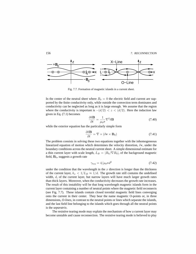
156 7. RECONNECTION
z z
x x
+B0
jy L jy
−B0
X−Line
O−Line
Fig. 7.7. Formation of magnetic islands in a current sheet.
In the center of the neutral sheet whereB0 = 0 the electric field and current are sup-ported by the finite conductivity only, while outside the convection term dominates andconductivity can be neglected as long as it is large enough. We assume that the regionwhere the conductivity is important is−(d/2) < z < (d/2). Here the induction lawgiven in Eq. (7.1) becomes
∂δB∂t
=1
µ0σ∇2δB (7.40)
while the exterior equation has the particularly simple form
∂δB∂t
= ∇× (δv ×B0) (7.41)
The problem consists in solving these two equations together with the inhomogeneouslinearized equation of motion which determines the velocity distortion,δv, under theboundary conditions across the neutral current sheet. A simple dimensional estimate fora thin current layer with scale length,LB = |B0/∇B0|, of the background magneticfield,B0, suggests a growth rate
γtea = 4/µ0σd2 (7.42)
under the condition that the wavelength in thex direction is longer than the thicknessof the current layer,kx < 1/LB ≈ 1/d. The growth rate still contains the undefinedwidth, d, of the current layer, but narrow layers will have much larger growth ratesthan thick layers. Moreover, when the conductivity decreases the growth rate increases.The result of this instability will be that long wavelength magnetic islands form in thecurrent layer containing a number of neutral points where the magnetic field reconnects(see Fig. 7.7). These islands contain closed toroidal magnetic field lines convergingonto the current in their center. They bear the name magnetic O-points or, in threedimensions,O-lines, in contrast to the neutral points or lines which separate the islands,and the last field line belonging to the islands which goes through all the neutral pointsis theseparatrix.
The resistive tearing mode may explain the mechanism of how a current layer maybecome unstable and cause reconnection. The resistive tearing mode is believed to play
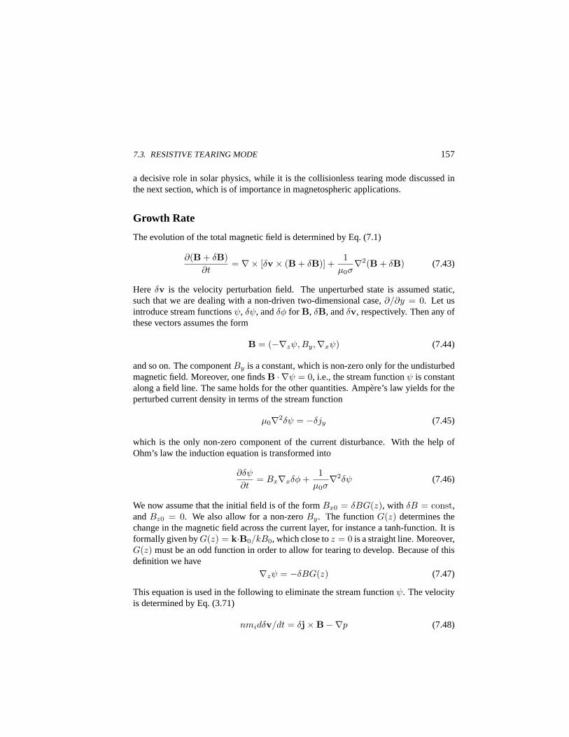
7.3. RESISTIVE TEARING MODE 157
a decisive role in solar physics, while it is the collisionless tearing mode discussed inthe next section, which is of importance in magnetospheric applications.
Growth Rate
The evolution of the total magnetic field is determined by Eq. (7.1)
∂(B + δB)∂t
= ∇× [δv × (B + δB)] +1
µ0σ∇2(B + δB) (7.43)
Here δv is the velocity perturbation field. The unperturbed state is assumed static,such that we are dealing with a non-driven two-dimensional case,∂/∂y = 0. Let usintroduce stream functionsψ, δψ, andδφ for B, δB, andδv, respectively. Then any ofthese vectors assumes the form
B = (−∇zψ, By,∇xψ) (7.44)
and so on. The componentBy is a constant, which is non-zero only for the undisturbedmagnetic field. Moreover, one findsB · ∇ψ = 0, i.e., the stream functionψ is constantalong a field line. The same holds for the other quantities. Ampere’s law yields for theperturbed current density in terms of the stream function
µ0∇2δψ = −δjy (7.45)
which is the only non-zero component of the current disturbance. With the help ofOhm’s law the induction equation is transformed into
∂δψ
∂t= Bx∇xδφ +
1µ0σ
∇2δψ (7.46)
We now assume that the initial field is of the formBx0 = δBG(z), with δB = const,andBz0 = 0. We also allow for a non-zeroBy. The functionG(z) determines thechange in the magnetic field across the current layer, for instance a tanh-function. It isformally given byG(z) = k·B0/kB0, which close toz = 0 is a straight line. Moreover,G(z) must be an odd function in order to allow for tearing to develop. Because of thisdefinition we have
∇zψ = −δBG(z) (7.47)
This equation is used in the following to eliminate the stream functionψ. The velocityis determined by Eq. (3.71)
nmidδv/dt = δj×B−∇p (7.48)
158 7. RECONNECTION
wherep is the pressure which does not play a role in the incompressible case we con-sider. Linearizing and introducing the following ansatz for the stream functions
[δψ
δφ
]=
[δψ0(z) cos(kxx)δg(z)γ(kxδB)−1 sin(kxx)
]exp(γt) (7.49)
the whole system of linearized equations for the stream functions, resulting from theincompressible equation of motion, the induction law, and Ohm’s law, can be reducedafter some tedious algebra to two coupled linear equations
δψ0 −Gδg =1
γτd
(d2δψ0
dz2− κ2δψ0
)
−γ2κ−2τ2A
(d2δg
dz2− κ2δg
)= G
(d2δψ0
dz2− κ2δψ0
)− δψ0
d2G
dz2
(7.50)
for δψ andδg, where we definedκ = kxd, the Alfven time
τA = d/vA (7.51)
and used the diffusion time given in Eq. (7.2). Moreover, the coordinates are madedimensionless by definingz → z/d. In the external region these equations, neglectingresistivity, yieldτd →∞ andδψ0 = Gδg and thus
G
(d2δψ0
dz2− κ2δψ0
)= δψ0
d2G
dz2(7.52)
We specify the external field by choosingG(z) = tanh z and find for the solutionsbelow and above the current sheet
δψ0+(+|z|) =(1 + κ−1tanh z
)exp(−κz)
δψ0−(−|z|) =(1− κ−1tanh z
)exp(κz)
(7.53)
The boundary conditions areδψ0± → 1 at the center of the current sheet,z → 0.The derivative,dδψ0/dz = δψ′0, of δψ0 stays discontinuous here. If we use∆ =[δψ′0+ − δψ′0−]z=0/δψ0(0), we obtain for the jump in the derivative ofδψ0
∆ = 2(1− κ2)/κ (7.54)
Now solve for the interior of the dissipation region. Since this region is very narrow,δψwill be constant inside. Moreover,G = tanh z ≈ z here. Furthermore, the wavelengthof the tearing mode is much larger than the width of the diffusion region, such thatκ2|δψ0| ¿ |d2δψ0/dz2| and κ2|δg| ¿ |d2δg/dz2|. This requirement reduces the
7.3. RESISTIVE TEARING MODE 159
differential equations forδψ0 andδg to
d2δψ0
dz2= γτd [δψ0(0)− zδg]
d2δψ0
dz2=
γ2τ2A
κ2
1z
d2δg
dz2
(7.55)
The matching condition demands that the derivatives ofδψ0 account for the abovejump∆ at the boundary of the dissipation region,z = 1. We integrate the second of theabove equations with respect toz over the dissipation layer to obtain the jump in thederivative expressed in terms ofg(z), divide by the constantδψ0(0) in the inner regionand compare with∆ to obtain
∆ = − γ2τ2A
δψ(0)κ2
∞∫
−∞
dz
z
d2δg
dz2(7.56)
This is the matching condition. In order to find its explicit form one must solve forg(z). This is achieved in the following way. One eliminates the second derivative ofδψ from the two differential equations (7.55) and transforms the resulting differentialequation into the simple form
y′′ + q2y = q (7.57)
where the prime indicates differentiation with respect toq = z(κ2τd/γτ2A)1/4, and
y = −δgq/δψ0(0). As q →∞ the functiony → −1/q.The solution of the above differential equation can be expressed as a definite inte-
gral. The matching condition (7.56) requires integration overy′′. Hence, we get
∆ = γ5/4τ3/4d τ
1/2A κ−1/2I (7.58)
whereI =∫∞−∞ y′′dq/q is a numerical value. The equation for the growth rateγ, i.e.,
the dispersion relation, is obtained by combining this formula with the expression for∆ obtained from Eq. (7.54). Numerical solutions have shown that it is sufficient toput q = 2 for the halfwidth of the diffusion region. Combining all the variables oneultimately obtains for the growth rate
γtea =1τd
[2(1− κ2)Iκ1/2
]4/5(τd
τA
)2/5
(7.59)
This is the general expression for the resistive tearing mode growth rate in a narrowplane current sheet of the particular shape given by the functionG(z). Due to constancyinside the layer, it diverges forκ = 0. A more precise calculation leads toκmax =
160 7. RECONNECTION
(4τA/τd)1/4 and a maximum growth rate
γtea,max ≈ (2τAτd)−1/2 (7.60)
This growth rate depends on the inverse of the diffusive and Alfven times in the currentlayer. Large diffusive and Alfven times will decrease it. In the magnetosphere andsolar wind the diffusive times are very long. Hence, resistive tearing will not playan important role. One must consider collisionless wave-particle interactions as therelevant processes for initiating fast reconnection here.
7.4. Collisionless Tearing Mode
When the plasma is collisionless, reconnection can evolve only as kinetic instabilitywith ion inertia as the force which mixes the magnetic fields. The resulting instabilityis thecollisionless tearing instability.
Configuration
As in the case of resistive tearing consider a planar current sheet (see Fig. 7.7), but noresistivity. A small disturbance in the position of the distribution of the current filamentsalongx will cause the filaments to attract each other and magnetic islands will start toform spontaneously. In a two-dimensional current sheet the magnetic field field is fullydescribed by the only non-vanishing component of the vector potential,Ay, as
B(x, z) =(−∂Ay
∂z, 0,
∂Ay
∂x
)(7.61)
Initially the magnetic field is a Harris-type field with noBz component (see Fig. 7.2in our companion book). The tearing mode will produce a periodic variation alongx.Hence, the distorted electric and vector potentials can be represented as plane waves
δAy(x, z, t) = δA(z) exp(−iωt + ikx)δφ(x, z, t) = δΦ(z) exp(−iωt + ikx)
(7.62)
It is most convenient to use the energy principle, derived in Sec. 3.6, to the evolution ofthe instability. In this simple two-dimensional case, it can be written as the energy bal-ance between the magnetic fluctuation energy and the energy dissipated by the currentin the Harris sheet
12µ0
∂
∂t
∫|δB|2 dz = −
∫δj · δE∗dz (7.63)
7.4. COLLISIONLESS TEARING MODE 161
where the asterisk indicates the conjugate complex of the electric wave field. The right-hand side is the Ohmic loss in the reconnecting current sheet. It accounts for the growthor damping of the magnetic field.
Electron Tearing Instability
Let us use a slightly modified Harris equilibrium with the magnetic field given as
B0 = exB0 tanh(z/d) + B0zez (7.64)
where the zero-order normal component of the magnetic field is small such that the ionsbehave unmagnetized in this component while the electrons are magnetized, implying
rge
d<
(B0z
B0
)2
<rgi
d(7.65)
Intuitively one may argue that the strong magnetization of the electrons in the fieldB0z
will introduce some stiffness of the magnetic field and thus a stabilizing effect on theelectron-driven tearing mode, theelectron tearing instability. In addition, the half widthof the current layer,∆, is assumed to be larger than the ion gyroradius
∆2 < rgid (7.66)
Electrons will thus be strongly magnetized while the ions are weakly magnetized.With the help of the above definitions the zero-order undisturbed but inhomoge-
neous particle distribution functions are
fs0(v, z) =n0
π3/2v3ths
exp[−v2 + v2
ds
v2ths
+2msvds(vy + qsA0y)
kBTs− qsφ0
kBTs
](7.67)
where the diamagnetic drift velocity in the density gradient of the Harris current layerof halfwidthd = Ln has been introduced as
vds = −kBTs/qsB0Ln (7.68)
Solving the linearized Vlasov equation for the disturbanceδfs of the particle distribu-tion functions using the representations of the electric and magnetic fields through thepotentials yields
δfs(v, z, t) =qsf0s
kBTs
[vdsδAy − δφ + iω
∫ t
−∞(vyδAy − δφ)dt′
](7.69)
As usual, the integration overt′ must be performed along the undisturbed particle orbits.This requires the solution of the undisturbed particle motion inside and outside the
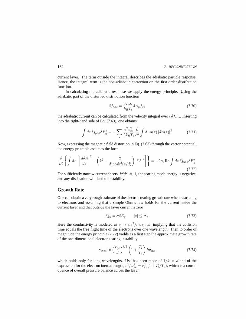
162 7. RECONNECTION
current layer. The term outside the integral describes the adiabatic particle response.Hence, the integral term is the non-adiabatic correction on the first order distributionfunction.
In calculating the adiabatic response we apply the energy principle. Using theadiabatic part of the disturbed distribution function
δfads =qsvds
kBTsδAyf0s (7.70)
the adiabatic current can be calculated from the velocity integral overvδfads. Insertinginto the right-hand side of Eq. (7.63), one obtains
∫dz δjyadδE∗
y = −∑
s
e2v2ds
2kBTs
∂
∂t
∫dz n(z) |δA(z)|2 (7.71)
Now, expressing the magnetic field distortion in Eq. (7.63) through the vector potential,the energy principle assumes the form
∂
∂t
∫dz
[∣∣∣∣dδA
dz
∣∣∣∣2
+(
k2 − 2d2cosh2(z/d)
)|δA|2
]= −2µ0Re
∫dz δjyadδE∗
y
(7.72)For sufficiently narrow current sheets,k2d2 ¿ 1, the tearing mode energy is negative,and any dissipation will lead to instability.
Growth Rate
One can obtain a very rough estimate of the electron tearing growth rate when restrictingto electrons and assuming that a simple Ohm’s law holds for the current inside thecurrent layer and that outside the layer current is zero
δjy = σδEy |z| ≤ ∆e (7.73)
Here the conductivity is modeled asσ ≈ ne2/mevthek, implying that the collisiontime equals the free flight time of the electrons over one wavelength. Then to order ofmagnitude the energy principle (7.72) yields as a first step the approximate growth rateof the one-dimensional electron tearing instability
γetea ≈(rge
d
)3/2(
1 +Ti
Te
)kvthe (7.74)
which holds only for long wavelengths. Use has been made of1/k > d and of theexpression for the electron inertial length,c2/ω2
pe = r2ge(1 + Ti/Te), which is a conse-
quence of overall pressure balance across the layer.
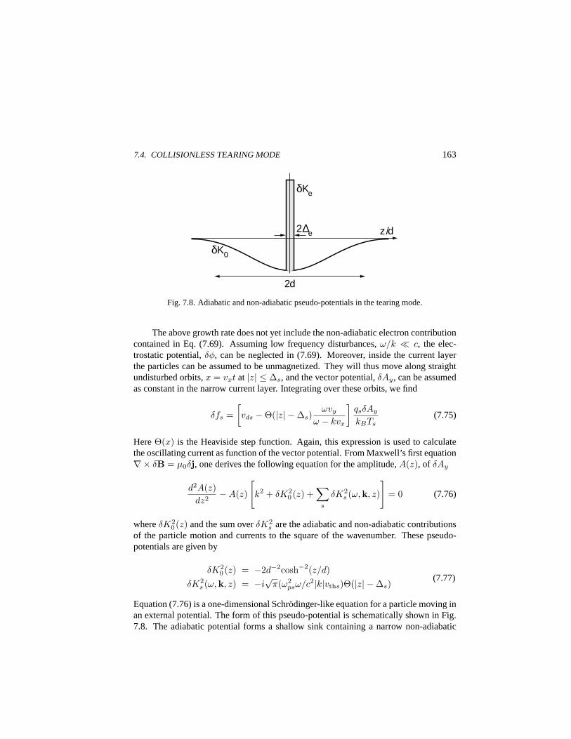
7.4. COLLISIONLESS TEARING MODE 163
δKe
2∆e z /d
2d
δK0
Fig. 7.8. Adiabatic and non-adiabatic pseudo-potentials in the tearing mode.
The above growth rate does not yet include the non-adiabatic electron contributioncontained in Eq. (7.69). Assuming low frequency disturbances,ω/k ¿ c, the elec-trostatic potential,δφ, can be neglected in (7.69). Moreover, inside the current layerthe particles can be assumed to be unmagnetized. They will thus move along straightundisturbed orbits,x = vxt at |z| ≤ ∆s, and the vector potential,δAy, can be assumedas constant in the narrow current layer. Integrating over these orbits, we find
δfs =[vds −Θ(|z| −∆s)
ωvy
ω − kvx
]qsδAy
kBTs(7.75)
HereΘ(x) is the Heaviside step function. Again, this expression is used to calculatethe oscillating current as function of the vector potential. From Maxwell’s first equation∇× δB = µ0δj, one derives the following equation for the amplitude,A(z), of δAy
d2A(z)dz2
−A(z)
[k2 + δK2
0 (z) +∑
s
δK2s (ω,k, z)
]= 0 (7.76)
whereδK20 (z) and the sum overδK2
s are the adiabatic and non-adiabatic contributionsof the particle motion and currents to the square of the wavenumber. These pseudo-potentials are given by
δK20 (z) = −2d−2cosh−2(z/d)
δK2s (ω,k, z) = −i
√π(ω2
psω/c2|k|vths)Θ(|z| −∆s)(7.77)
Equation (7.76) is a one-dimensional Schrodinger-like equation for a particle moving inan external potential. The form of this pseudo-potential is schematically shown in Fig.7.8. The adiabatic potential forms a shallow sink containing a narrow non-adiabatic
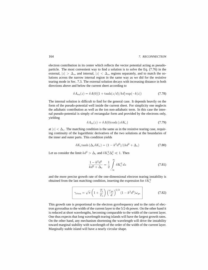
164 7. RECONNECTION
electron contribution in its center which reflects the vector potential acting as pseudo-particle. The most convenient way to find a solution is to solve the Eq. (7.76) in theexternal,|z| > ∆s, and internal,|z| < ∆s, regions separately, and to match the so-lutions across the narrow internal region in the same way as we did for the resistivetearing mode in Sec. 7.3. The external solution decays with increasing distance in bothdirections above and below the current sheet according to
δAex(z) = δA(0)[1 + tanh(z/d)/kd] exp(−k|z|) (7.78)
The internal solution is difficult to find for the general case. It depends heavily on theform of the pseudo-potential well inside the current sheet. For simplicity one neglectsthe adiabatic contribution as well as the ion non-adiabatic term. In this case the inter-nal pseudo-potential is simply of rectangular form and provided by the electrons only,yielding
δAin(z) = δA(0)cosh (zδKe) (7.79)
at |z| < ∆e. The matching condition is the same as in the resistive tearing case, requir-ing continuity of the logarithmic derivatives of the two solutions at the boundaries ofthe inner and outer parts. This condition yields
δKetanh (∆eδKe) = (1− k2d2)/(kd2 + ∆e) (7.80)
Let us consider the limitkd2 > ∆e andδK2e∆2
e ¿ 1. Then
1− k2d2
kd2 + ∆e=
12
∞∫
−∞δK2
e dz (7.81)
and the more precise growth rate of the one-dimensional electron tearing instability isobtained from the last matching condition, inserting the expression forδK2
e
γetea =√
π
(1 +
Ti
Te
) (rge
d
)5/2
(1− k2d2)ωge (7.82)
This growth rate is proportional to the electron gyrofrequency and to the ratio of elec-tron gyroradius to the width of the current layer to the 5/2-th power. On the other hand itis reduced at short wavelengths, becoming comparable to the width of the current layer.One thus expects that long wavelength tearing islands will have the largest growth rates.On the other hand, any mechanism shortening the wavelength will drive the instabilitytoward marginal stability with wavelength of the order of the width of the current layer.Marginally stable island will have a nearly circular shape.

7.4. COLLISIONLESS TEARING MODE 165
Ion Tearing Instability
So far we have neglected the effect of the small normal magnetic field component,B0z,on the evolution of the one-dimensional tearing instability. Realistic current sheets andequilibria are always two-dimensional with non-vanishing normal magnetic fields andthe magnetic field across the sheet will never turn exactly zero in any place. As wealready mentioned, the bulk low-energy electron component will in such a case becomestrongly magnetized in theB0z field component in the center of the magnetic neutralsheet. It will stay frozen-in and not allow the electron tearing mode to become unstable.In such cases the ions drive the instability due to their larger inertia and unmagnetizednature, if their gyroradius is large enough across the current sheet. A calculation verysimilar to that presented in the previous section leads to the growth rate of the one-dimensionalion tearing instability
γitea ≈√
π(rgi
d
)5/2(
1 +Te
Ti
)(1− k2d2)ωgi (7.83)
This growth rate scales as the ion-cyclotron frequency. It is positive as long as thetearing wavelength is longer than the halfwidth of the current sheet,k2d2 < 1. Thecorresponding mode grows much slower than the electron tearing mode and is of longerwavelength. Similarly, the marginally stable width of the islands will be of the orderof the ion gyroradius. Since the electron tearing mode is stabilized much earlier, itis reasonable to assume that the dominant tearing mode under collisionless conditionsis ion tearing driven by inertial effects. Whenkd increases beyond one, the mode isdamped. However, strongest damping occurs fork2d2 = 5. For current sheets of largerwidth the damping goes to zero again.
Two-Dimensional Tearing
However, because of the two-dimensionality of the problem, this is not the full story.One must take into account the energy contribution of the frozen-in magnetized elec-trons. This case corresponds to the range of ratios given in Eq. (7.65). The magnetizedelectrons perform a gyration about the normal magnetic field component,B0z, in thecurrent neutral sheet and a bounce motion between the two mirror points of the mag-netic field at the boundaries. Both motions are fast oscillations, which do not contributeto instability and can be averaged out when determining the electron motion. We arethus left with an effective average drift motion
δvex = δEy/Boz (7.84)
of the electrons in the bounce- and gyro-averaged electric wave field of the tearingmode. This value is inserted in the averaged electron continuity equation, and the wave
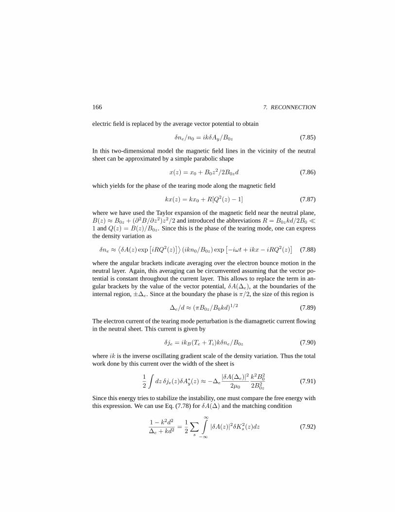
166 7. RECONNECTION
electric field is replaced by the average vector potential to obtain
δne/n0 = ikδAy/B0z (7.85)
In this two-dimensional model the magnetic field lines in the vicinity of the neutralsheet can be approximated by a simple parabolic shape
x(z) = x0 + B0z2/2B0zd (7.86)
which yields for the phase of the tearing mode along the magnetic field
kx(z) = kx0 + R[Q2(z)− 1] (7.87)
where we have used the Taylor expansion of the magnetic field near the neutral plane,B(z) ≈ B0z + (∂2B/∂z2)z2/2 and introduced the abbreviationsR = B0zkd/2B0 ¿1 andQ(z) = B(z)/B0z. Since this is the phase of the tearing mode, one can expressthe density variation as
δne ≈⟨δA(z) exp
[iRQ2(z)
]⟩(ikn0/B0z) exp
[−iωt + ikx− iRQ2(z)]
(7.88)
where the angular brackets indicate averaging over the electron bounce motion in theneutral layer. Again, this averaging can be circumvented assuming that the vector po-tential is constant throughout the current layer. This allows to replace the term in an-gular brackets by the value of the vector potential,δA(∆e), at the boundaries of theinternal region,±∆e. Since at the boundary the phase isπ/2, the size of this region is
∆e/d ≈ (πB0z/B0kd)1/2 (7.89)
The electron current of the tearing mode perturbation is the diamagnetic current flowingin the neutral sheet. This current is given by
δje = ikB(Te + Ti)kδne/B0z (7.90)
whereik is the inverse oscillating gradient scale of the density variation. Thus the totalwork done by this current over the width of the sheet is
12
∫dz δje(z)δA∗y(z) ≈ −∆e
|δA(∆e)|22µ0
k2B20
2B20z
(7.91)
Since this energy tries to stabilize the instability, one must compare the free energy withthis expression. We can use Eq. (7.78) forδA(∆) and the matching condition
1− k2d2
∆e + kd2=
12
∑s
∞∫
−∞|δA(z)|2δK2
s (z)dz (7.92)

7.4. COLLISIONLESS TEARING MODE 167
to obtain the condition for instability in the particular form
1− k2d2
k2∆ed(kd + ∆e/d)>
12
B20
B20z
(7.93)
This condition implies that the compression energy of the plasma in the narrow currentlayer is not large enough to exceed the free energy, if
rge/d < B0z/B0 < (rge/d)1/2 (7.94)
In this case most of the electrons drift along thex direction inside the neutral sheet ofsize∆e ≈
√rged, while exhibiting a bounce oscillation between the boundaries of the
neutral sheet and performing a gyratory motion in the normal field,B0z. The smallthickness of the electron current layer allows to neglect∆e ¿ d againstd to obtain
1k2d2
− 1 >
(B0
B0z
)2 (rge
d
)1/2 kd
2(7.95)
as condition of instability. Under these favorable conditions, the ion tearing instabilitywill grow at the growth rate in Eq. (7.83) whenever the growth rate exceeds the value
γitea = γ′ωgi(1− k2d2) > ωgiB0z/B0 (7.96)
with γ′ =√
π (rgi/d)5/2(1 + Te/Ti). Eqs. (7.95) and (7.96) set thresholds on the iontearing instability: a large normal component of the magnetic field in the center of theneutral sheet tends to stabilize the collisionless tearing mode. To visualize the unstablerange we combine the conditions into one, definingb = (B0z/B0). Then instabilityarises for
γ′(1− k2d2) > b > (kd)3/2(1− k2d2)−1/2(rge/d)1/4 (7.97)
The graphic representation of this condition is shown in Fig. 7.9. For givenb andγ′ in-stability arises in the shaded region. Hence, there is a restricted domain of wavenumbersand of normal magnetic field components, depending on the electron and ion gyroradii,where the ion tearing mode can develop.
Magnetospheric Substorms
The collisionless ion tearing mode is part of the most successful substorm model (seeSec. 5.6 of our companion book). Under quiet conditions the magnetic field in the centerof the Earth’s plasma sheet is dipolar, with a relatively large non-negligible normalcomponent,B0z, and the tearing mode is stabilized by the pressure of the electronstrapped in the center of the neutral sheet. In the substorm growth phase new open
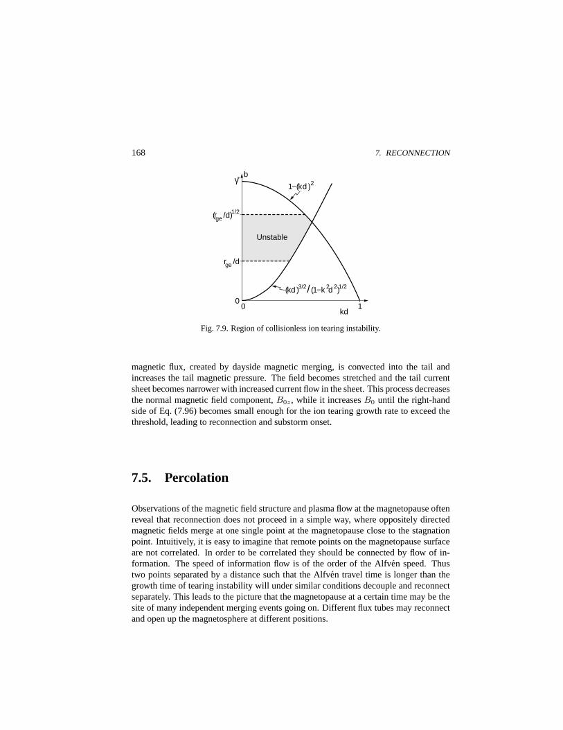
168 7. RECONNECTION
γ"
0 0
1−(kd )2
Unstable
(kd )3/2/ (1−k 2d 2)1/2
b
1 kd
rge /d
(rge /d)1/2
Fig. 7.9. Region of collisionless ion tearing instability.
magnetic flux, created by dayside magnetic merging, is convected into the tail andincreases the tail magnetic pressure. The field becomes stretched and the tail currentsheet becomes narrower with increased current flow in the sheet. This process decreasesthe normal magnetic field component,B0z, while it increasesB0 until the right-handside of Eq. (7.96) becomes small enough for the ion tearing growth rate to exceed thethreshold, leading to reconnection and substorm onset.
7.5. Percolation
Observations of the magnetic field structure and plasma flow at the magnetopause oftenreveal that reconnection does not proceed in a simple way, where oppositely directedmagnetic fields merge at one single point at the magnetopause close to the stagnationpoint. Intuitively, it is easy to imagine that remote points on the magnetopause surfaceare not correlated. In order to be correlated they should be connected by flow of in-formation. The speed of information flow is of the order of the Alfven speed. Thustwo points separated by a distance such that the Alfven travel time is longer than thegrowth time of tearing instability will under similar conditions decouple and reconnectseparately. This leads to the picture that the magnetopause at a certain time may be thesite of many independent merging events going on. Different flux tubes may reconnectand open up the magnetosphere at different positions.
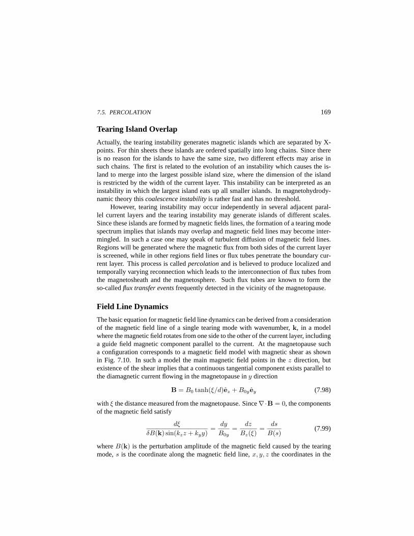
7.5. PERCOLATION 169
Tearing Island Overlap
Actually, the tearing instability generates magnetic islands which are separated by X-points. For thin sheets these islands are ordered spatially into long chains. Since thereis no reason for the islands to have the same size, two different effects may arise insuch chains. The first is related to the evolution of an instability which causes the is-land to merge into the largest possible island size, where the dimension of the islandis restricted by the width of the current layer. This instability can be interpreted as aninstability in which the largest island eats up all smaller islands. In magnetohydrody-namic theory thiscoalescence instabilityis rather fast and has no threshold.
However, tearing instability may occur independently in several adjacent paral-lel current layers and the tearing instability may generate islands of different scales.Since these islands are formed by magnetic fields lines, the formation of a tearing modespectrum implies that islands may overlap and magnetic field lines may become inter-mingled. In such a case one may speak of turbulent diffusion of magnetic field lines.Regions will be generated where the magnetic flux from both sides of the current layeris screened, while in other regions field lines or flux tubes penetrate the boundary cur-rent layer. This process is calledpercolationand is believed to produce localized andtemporally varying reconnection which leads to the interconnection of flux tubes fromthe magnetosheath and the magnetosphere. Such flux tubes are known to form theso-calledflux transfer eventsfrequently detected in the vicinity of the magnetopause.
Field Line Dynamics
The basic equation for magnetic field line dynamics can be derived from a considerationof the magnetic field line of a single tearing mode with wavenumber,k, in a modelwhere the magnetic field rotates from one side to the other of the current layer, includinga guide field magnetic component parallel to the current. At the magnetopause sucha configuration corresponds to a magnetic field model with magnetic shear as shownin Fig. 7.10. In such a model the main magnetic field points in thez direction, butexistence of the shear implies that a continuous tangential component exists parallel tothe diamagnetic current flowing in the magnetopause iny direction
B = B0 tanh(ξ/d)ez + B0yey (7.98)
with ξ the distance measured from the magnetopause. Since∇·B = 0, the componentsof the magnetic field satisfy
dξ
δB(k) sin(kzz + kyy)=
dy
B0y=
dz
Bz(ξ)=
ds
B(s)(7.99)
whereB(k) is the perturbation amplitude of the magnetic field caused by the tearingmode,s is the coordinate along the magnetic field line,x, y, z the coordinates in the
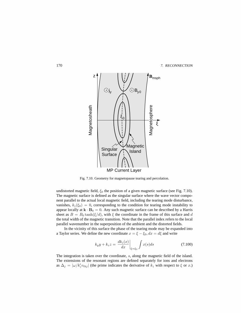
170 7. RECONNECTION
jy By0
Magnetic Island Singular
Surface
ξ
z Bmsph
Mag
neto
shea
th
Mag
neto
sphe
re
MP Current Layer
ξ0
Fig. 7.10. Geometry for magnetopause tearing and percolation.
undistorted magnetic field,ξ0 the position of a given magnetic surface (see Fig. 7.10).The magnetic surface is defined as the singular surface where the wave vector compo-nent parallel to the actual local magnetic field, including the tearing mode disturbance,vanishes,k‖(ξ0) = 0, corresponding to the condition for tearing mode instability toappear locally atk ·B0 = 0. Any such magnetic surface can be described by a Harrissheet asB = B0 tanh(ξ/d), with ξ the coordinate in the frame of this surface anddthe total width of the magnetic transition. Note that the parallel index refers to the localparallel wavenumber in the superposition of the ambient and the distorted fields.
In the vicinity of this surface the phase of the tearing mode may be expanded intoa Taylor series. We define the new coordinatex = ξ − ξ0, dx = dξ and write
kyy + kzz =dk‖(x)
dx
∣∣∣∣ξ=ξ0
∫x(s)ds (7.100)
The integration is taken over the coordinate,s, along the magnetic field of the island.The extensions of the resonant regions are defined separately for ions and electronsas∆j = |ω/k′‖vthj | (the prime indicates the derivative ofk‖ with respect toξ or x.)
7.5. PERCOLATION 171
Integrating the above equation yields the result
x = ±
2δB(k)k′‖B0
[2λ2 − 1− cos
(k′‖
∫x(s)ds
)]1/2
(7.101)
The integration constantλ2 determines whether the magnetic surfaces are open,λ >1, or closed,λ < 1. The separatrix between open and closed island field lines isdetermined by the conditionλ = 1. This yields the halfwidth of the islands of a givenwavenumber,k, at the particular resonant surface position
w(ξ0,k) = 2[δB(k)/B0k′‖(ξ0,k)]1/2 (7.102)
This width is a function of the position,ξ0, of the singular resonant layer, the centerof the magnetic surface. In addition it depends on the wavenumber. Hence, it can bedifferent for different layers and wavenumbers. The widths form an entire spectrum ofdifferent lengths and magnetic islands belonging to different layers may overlap. Fortwo different islands at the resonant surfaces,ξ01 andξ02, the overlap condition is
w1(ξ01,k1) + w2(ξ02,k2) > |ξ01 − ξ02| (7.103)
Migration Coefficient
Whenever this condition is satisfied, the two magnetic surfaces cease to exist separatelybut belong to both islands at the same time. The magnetic field lines of these twoislands mix, the common surface and the field lines start migrating across the islandsand the layers. This process is comparable to some kind of Brownian motion with aspatial step,∆x ≈ w, performed during a characteristic stepping time,τw = s/v,wherev is a characteristic velocity of a magnetic perturbation. The length of the fieldline corresponding to one Brownian step is estimated by
sw ≈ (k′‖w)−1 (7.104)
Using this expression for the width of the islands allows to define a geometric field linemigration coefficient. This coefficient has the dimension of a length
Dgeo ≈ w2
sw≈
∣∣∣∣δB(k)|k′‖|1/3B0
∣∣∣∣3/2
(7.105)
In this expression the magnetic fluctuation spectrum,[δB(k)]2, appears.The geometric migration coefficient can be rewritten with the help of the total
turbulent magnetic energy,Wtea =∑
k |δB(k)|2/B20 , normalized to the undisturbed
magnetic energy. The number of islands in the total layer isN ≈ d/〈w〉, where〈w〉 ≈

172 7. RECONNECTION
w is the average width of the islands. This yields for the normalized turbulent magneticenergy density in the shear tearing mode:
Wtea ≈ N(δB/B0)2 ≈ w3k′2‖ d (7.106)
which is approximately the normalized energy released during the shear tearing modeinstability under the condition that many modes are excited. The geometric field linediffusion coefficient can now be expressed as
Df,geo ≈ Wtea
|k′‖|d≈ π
∑
k
[ |δB(k)|2B2
0
]δ[k‖(x)] (7.107)
This version of the migration coefficient is the quasilinear resonant diffusion coefficientof migrating field lines, valid for random phase interactions between the overlappingmodes. Hence, the overlap of the islands can be interpreted as a randomization of fieldlines whenever the tearing mode islands overlap.
Some of the magnetic flux tubes will start migrating across the current layer, lead-ing to interconnected magnetosheath-magnetosphere flux tubes which appear as fluxtransfer events in magnetic recordings. Figure 7.11 illustrates such an overlap and howa magnetic flux tube may locally penetrate across the magnetopause current layer form-ing a flux transfer event. The number of singular surfaces and X-points along theξ axisacross the magnetopause boundary layer is always an odd number and in the overlapregions the local magnetic field is amplified. Because of the finite shear component,B0y 6= 0, the magnetic field in the X-points is not zero. Only thez components of themagnetic field cancel each other. A flux tube will usually enter as aB0y-tube throughone of the X-points on one side and turn around the overlapping islands until it leavesfrom an X-point on the other side of the current layer. Hence, any migrating flux tubewill constitute a three-dimensional entity.
The geometric field line diffusion coefficient does not have the dimension of adiffusion coefficient. In order to get a real diffusion coefficient, one has to multiplyDf,geo by the characteristic velocity,v, of a magnetic perturbation. The appropriatespeed is the Alfven velocity. Hence, overlap of magnetic island will cause migration ofmagnetic field field lines corresponding to a percolation diffusion coefficient
Dper ≈ vAWtea/|k′‖|d (7.108)
This diffusion coefficient can be applied only to magnetic flux tube diffusion and onlyto those regions where islands overlap. Particle diffusion is not described by it.
As already mentioned earlier, stabilization of the tearing mode will occur when theisland width becomes comparable to the ion gyroradius,w ≈ rgi. Thus the diffusioncoefficient at stabilization is proportional to the third power of the ion gyroradius. If we

7.5. PERCOLATION 173
FTE
−B0z
B0y
B0z
X1
X2 X3
0 ξ1 ξ2 ξ3 ξ
Fig. 7.11. Percolation in tearing island overlap.
replace the derivative of the singular wavenumber byk′‖ ≈ kB0/B0yd, the percolationdiffusion coefficient at saturation
Dper,sat ≈vAkr3
gi
d
B0
B0y(7.109)
assumes a particularly simple form which is valid as long as the shear component of themagnetic field has a finite value,B0y. For vanishing shear, percolation ceases to existand the character of the tearing mode changes.
Concluding Remarks
Reconnection is one particular and very fruitful concept of fast and localized magneticfield line diffusion. It is based on two assumptions. The first assumption is that the
174 7. RECONNECTION
two interacting magnetic fields possess antiparallel components which may annihilatewhen contacting each other. The second assumption is that in the region of contactsome mechanism exists which decouples the plasma from the field. In magnetohydro-dynamics, the model where reconnection is best studied, decoupling can be achievedby resistive interactions among the particles. From a naive point of view they are thusnot applicable to conditions at the magnetopause or in most space plasmas. But thisview is incorrect insofar as locally in many cases anomalous collisions may be gener-ated nonlinearly. We will discuss such possibilities in Chap. 12 below. The anomalouscollisions replace the particle collisions and may cause local resistive reconnection.
Collisionless reconnection is based on more realistic plasma models which includethe different inertia of electrons and ions. The latter may decouple the particles fromthe field and allow for field line rearrangements. The electrons are very sensitive to thepresence of normal magnetic fields in the reconnection site and may cause stabilization.But ion inertia may still provide sufficient slip of the magnetic field for reconnection tobe maintained. Magnetic shear is important and may lead to island overlap and mag-netic field migration giving rise to the formation of flux transfer events at the daysidemagnetopause and flux ropes in the magnetotail.
Further Reading
Reconnection in magnetohydrodynamics is reviewed in [1] and [3]. Magnetohydrody-namic aspects of reconnection including simulations are described by Biskamp,Phys.Reps., 237(1994) 179. Collisional reconnection has been reviewed by White in [4]. Thestationary collisionless reconnection theory is taken from Vekstein and Priest,Phys.Plasmas2 (1995) 3169. In the theory of the collisionless tearing mode we followed[2]. The section about percolation theory is based on Galeev et al.,Space Sci. Rev.44(1986) 1.
[1] D. Biskamp, Nonlinear Magnetohydrodynamics(Cambridge University Press,Cambridge, 1993).
[2] A. A. Galeev, inMagnetospheric Plasma Physics, edited by A. Nishida (D. ReidelPubl. Co., Dordrecht, 1982), p. 143.
[3] E. Priest,Solar Magnetohydrodynamics(D. Reidel Publ. Co., Dordrecht, 1984).
[4] M. N. Rosenbluth and R. Z. Sagdeev,Handbook of Plasma Physics, Vol. 1: BasicPlasma Physics I, edited by A. A. Galeev and R. N. Sudan (North-Holland Publ.Co., Amsterdam, 1983), p. 611.
8. Wave-Particle Interaction
With this chapter we enter the field ofnonlinear effectsin space plasma physics. Wehave chosen to split the discussion of the nonlinear effects into two parts. The first part(Chaps. 8–9) discusses weakly turbulent effects, which are usually dealt with by usingperturbation theory, while the second part (Chaps. 10–11) concentrates on stronglyturbulent phenomena. Chapter 12 concludes this volume with a number of selectedapplications of nonlinear space plasma theory.
The presentation of the nonlinear theory differs from that of linear theory in thatit is more review-like than tutorial. The reason for this difference is twofold. Plasmaphysics is fundamentally nonlinear. Linear theory illuminates only a narrow windowout of the wealth of all effects which can proceed in a plasma. Mathematically, lineartheory uses a well-developed apparatus of algorithms. Naturally, for the much widerfield of nonlinear theory no such general algorithms are available.
While discussing the linear aspects of space plasma physics has filled our compan-ion bookBasic Space Plasma Physicsand the first half of the present volume, describ-ing the nonlinearities in comparable depth would expand this presentation to unreason-able size. Even if we wanted, it would be impossible, because nonlinear plasma physicsis still, after 35 years of intensive research, in its infancy. Few analytical methods areknown to treat nonlinear effects, and most of these methods rely on approximationsand lowest-order perturbation theory. This methodological lack of a general nonlineartheory and the difficulties and restrictions of nonlinear analytical methods have drivenmost researchers into the partly qualitative field of numerical simulations.
The present chapter starts with describing the primary effect of large amplitudewaves on the particle orbits, leading toparticle trapping in a wave, followed by adiscussion ofexact nonlinear waves, which can be calculated in a one-dimensionalelectrostatic plasma in the kinetic approximation. Then we present the theory ofweakturbulenceor weakwave-particle interaction, and a discussion ofquasilinear theoryfor different types of waves, the today still most important part in space plasma appli-cations. We continue with an application of this theory topitch angle diffusion. Thefinal sections deal with a brief introduction intowave-wave interaction, in the two ap-proximations ofcoherentandincoherentinteractions, and its application to solar radiobursts.
175
176 8. WAVE-PARTICLE INTERACTION
8.1. Trapping in Single Waves
The simplest nonlinear effect is particle trapping. When a plasma wave reaches largeamplitudes, either because it has been injected at large amplitude into the plasma byexternal means or because it has grown to large amplitude due to instability, severalentirely new effects set in. The first and simplest one is particle trapping in the potentialfield of the wave.
Particles Trapped in a Well
Consider, for instance, a potential well created by an ion in a plasma. In the fluiddescription electrons in the vicinity of the ion will readily deplete this well outside theDebye radius,λD. But if one takes into account the different velocities of the electrons,say, in a Maxwellian distribution of particles, it becomes clear that only low energyelectrons will be trapped in the vicinity of the ion in the potential trough. The conditionfor trapping is that the particle energy is less than the potential energy of the electricfield, We < e|φ|. The particle distribution then splits into a trapped and a non-trappeddistribution. In a shallow potential well it is reasonable to assume that the trappeddistribution is constant,ftr(We) = fe(0), wherefe(0) is the distribution at the centerof the well. The particle density is calculated from the moment of the distributionfunction as
ne(φ) = 2n0
[∫ ∞
ξ
fe(We, φ)dv +∫ ξ
0
fe(0)dv
](8.1)
andξ = (2eφ/me)1/2. The factor 2 takes care of the symmetry of distribution functionand potential well. It is reasonable to choose a Boltzmann distribution for the electrondistribution function
fe(W,φ) =(me
2πmekBTe)1/2exp
(−We − eφ
kBTe
)(8.2)
Calculating the integrals, one finds that the density can be represented as a sum of threeterms which depend onψ = eφ/kBTe
ne(ψ) = n0
[1− erf(ψ1/2)
]eψ + 2(ψ/π)1/2
(8.3)
Here the functionerf(x) is Gauss’ error integral
erf(x) =2
π1/2
∫ x
0
exp(−t2)dt (8.4)
8.1. TRAPPING IN SINGLE WAVES 177
For very shallow potentials and potential energies much less than the electron thermalenergy, the integral can be expanded in the small-amplitude limit to obtain
ne(φ) = n0
[1 +
eφ
kBTe− 4
3π1/2
(eφ
kBTe
)3/2]
(8.5)
This expression shows that to lowest order the dependence of the density on the poten-tial is a linear function. However, due to the trapping of particles, another nonlinearterm comes into play.
For large argument,ξ ∝ ψ À 1, the first two terms in the full expression of thedensity cancel because the error function becomes unity. The density is determinedentirely by the trapped particle component
ne = 2n0
(eφ
πkBTe
)1/2
(8.6)
The density increases only as the half power of the potential, yielding a weaker depen-dence on the potential than in the Boltzmann case.
Particle Trapping in a Monochromatic Wave
Similarly, particles can become trapped in a wave potential if the particle kinetic energyin the wave frame is less than the potential energy of the wave. It is immediately clearthat trapping will be largest for resonant particles moving at approximately the samevelocity as the wave and experiencing a nearly stationary electric wave potential
φ(x, t) = φ0 cos(kx− ωt) = φ0 cos(kx′) (8.7)
where the wave coordinates have been transformed into the wave frame by
x′ = x− (ω/k)t (8.8)
The particle velocity also transforms and becomes
v′ = v − ω/k (8.9)
such that the total energy of the particle in the wave frame of reference is
We = 12mv′2 − eφ0 cos kx′ (8.10)
When considering the motion of the electron in the two-dimensional particle phasespace(x′, v′), the particle moves along the lines of constant energyWe. Figure 8.1shows the schematic form of these lines. There are two families of curves in this phase
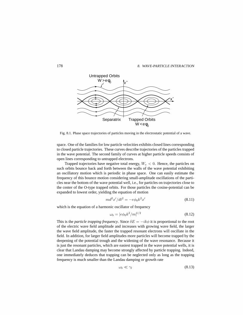
178 8. WAVE-PARTICLE INTERACTION
v"
Untrapped Orbits W >eφ0
Trapped Orbits W <eφ0
Separatrix
x"
Fig. 8.1. Phase space trajectories of particles moving in the electrostatic potential of a wave.
space. One of the families for low particle velocities exhibits closed lines correspondingto closed particle trajectories. These curves describe trajectories of the particles trappedin the wave potential. The second family of curves at higher particle speeds consists ofopen lines corresponding to untrapped electrons.
Trapped trajectories have negative total energy,We < 0. Hence, the particles onsuch orbits bounce back and forth between the walls of the wave potential exhibitingan oscillatory motion which is periodic in phase space. One can easily estimate thefrequency of this bounce motion considering small-amplitude oscillations of the parti-cles near the bottom of the wave potential well, i.e., for particles on trajectories close tothe center of the O-type trapped orbits. For those particles the cosine-potential can beexpanded to lowest order, yielding the equation of motion
md2x′/dt2 = −eφ0k2x′ (8.11)
which is the equation of a harmonic oscillator of frequency
ωb = |eφ0k2/m|1/2 (8.12)
This is theparticle trapping frequency. SinceδE = −ikφ it is proportional to the rootof the electric wave field amplitude and increases with growing wave field, the largerthe wave field amplitude, the faster the trapped resonant electrons will oscillate in thefield. In addition, for larger field amplitudes more particles will become trapped by thedeepening of the potential trough and the widening of the wave resonance. Because itis just the resonant particles, which are easiest trapped in the wave potential wells, it isclear that Landau damping may become strongly affected by particle trapping. Indeed,one immediately deduces that trapping can be neglected only as long as the trappingfrequency is much smaller than the Landau damping or growth rate
ωb ¿ γl (8.13)
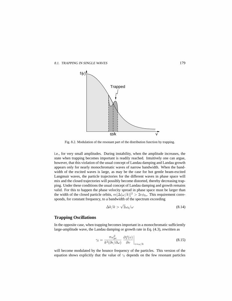
8.1. TRAPPING IN SINGLE WAVES 179
Trapped
f (v)
v ω /k
Fig. 8.2. Modulation of the resonant part of the distribution function by trapping.
i.e., for very small amplitudes. During instability, when the amplitude increases, thestate when trapping becomes important is readily reached. Intuitively one can argue,however, that this violation of the usual concept of Landau damping and Landau growthappears only for nearly monochromatic waves of narrow bandwidth. When the band-width of the excited waves is large, as may be the case for hot gentle beam-excitedLangmuir waves, the particle trajectories for the different waves in phase space willmix and the closed trajectories will possibly become distorted, thereby decreasing trap-ping. Under these conditions the usual concept of Landau damping and growth remainsvalid. For this to happen the phase velocity spread in phase space must be larger thanthe width of the closed particle orbits,m[∆(ω/k)]2 > 2eφ0,. This requirement corre-sponds, for constant frequency, to a bandwidth of the spectrum exceeding
∆k/k >√
2ωb/ω (8.14)
Trapping Oscillations
In the opposite case, when trapping becomes important in a monochromatic sufficientlylarge-amplitude wave, the Landau damping or growth rate in Eq. (4.3), rewritten as
γl =πω2
pe
k2(∂ε/∂ω)∂f(v)
∂v
∣∣∣∣v=ω/k
(8.15)
will become modulated by the bounce frequency of the particles. This version of theequation shows explicitly that the value ofγl depends on the few resonant particles
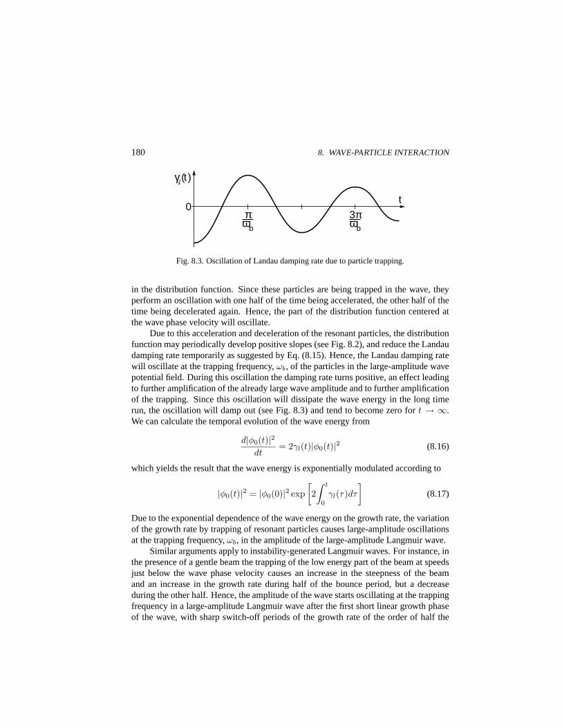
180 8. WAVE-PARTICLE INTERACTION
γ (t )
0
ωb
π 3π ωb
t
Fig. 8.3. Oscillation of Landau damping rate due to particle trapping.
in the distribution function. Since these particles are being trapped in the wave, theyperform an oscillation with one half of the time being accelerated, the other half of thetime being decelerated again. Hence, the part of the distribution function centered atthe wave phase velocity will oscillate.
Due to this acceleration and deceleration of the resonant particles, the distributionfunction may periodically develop positive slopes (see Fig. 8.2), and reduce the Landaudamping rate temporarily as suggested by Eq. (8.15). Hence, the Landau damping ratewill oscillate at the trapping frequency,ωb, of the particles in the large-amplitude wavepotential field. During this oscillation the damping rate turns positive, an effect leadingto further amplification of the already large wave amplitude and to further amplificationof the trapping. Since this oscillation will dissipate the wave energy in the long timerun, the oscillation will damp out (see Fig. 8.3) and tend to become zero fort → ∞.We can calculate the temporal evolution of the wave energy from
d|φ0(t)|2dt
= 2γl(t)|φ0(t)|2 (8.16)
which yields the result that the wave energy is exponentially modulated according to
|φ0(t)|2 = |φ0(0)|2 exp[2∫ t
0
γl(τ)dτ
](8.17)
Due to the exponential dependence of the wave energy on the growth rate, the variationof the growth rate by trapping of resonant particles causes large-amplitude oscillationsat the trapping frequency,ωb, in the amplitude of the large-amplitude Langmuir wave.
Similar arguments apply to instability-generated Langmuir waves. For instance, inthe presence of a gentle beam the trapping of the low energy part of the beam at speedsjust below the wave phase velocity causes an increase in the steepness of the beamand an increase in the growth rate during half of the bounce period, but a decreaseduring the other half. Hence, the amplitude of the wave starts oscillating at the trappingfrequency in a large-amplitude Langmuir wave after the first short linear growth phaseof the wave, with sharp switch-off periods of the growth rate of the order of half the
8.2. EXACT NONLINEAR WAVES 181
trapping frequency. In addition, because resonance is slightly shifted, it also becomespossible that the frequency of the Langmuir wave starts oscillating. However, these finestructure effects are difficult to detect in space plasmas.
8.2. Exact Nonlinear Waves
The former sections have made clear that trapping plays an important role in the non-linear evolution of plasma waves. In principle, when investigating the dynamics of suchwave from a kinetic point of view one should distinguish between two components ofthe particle distribution function, the trapped and the transmitted particles. Both dis-tributions are not independent neither mutually nor of the wave amplitude. They aredetermined by the Vlasov equation and the Poisson equation. The question arises then,under which conditions one can find exact solutions of this system of equations whichdetermine in a self-consistent way all three quantities.
The complex nonlinear equations describing the evolution of plasma waves canusually not be solved exactly. There is a very small number of occasions when suchsolutions can be constructed. The simplest one is in the magnetohydrodynamic ap-proximation, where it can be demonstrated that incompressible Alfven waves in idealmagnetohydrodynamics also exist at large amplitudes. The more interesting question is,however, what kind of exact nonlinear waves can exist in a Vlasov plasma. Such wavesexist only in one-dimensional plasmas and are known asBernstein-Greene-Kruskalwavesor simply BGK modes.
BGK Modes
BGK modes are exact one-dimensional electrostatic solutions of the unmagnetized Vla-sov-Poisson system of equations. In the wave frame they are non-oscillating entitieswhich move at a certain velocity,v0 = const, across the plasma laboratory frame andcan be considered as large-amplitude stationary structures. Inside these structures oneencounters an equilibrium between the particles and the waves, the stability of whichagainst external disturbances can be considered separately. It is of considerable interestthat the plasma allows such structures to exist for comparably long times.
If a one-dimensional system of Vlasov-Poisson equations is transformed by re-placingx → x − v0t andv → v − v0 to a stationary moving system,∂/∂t → 0, thenow stationary distribution function,fs0(x− v0t, v − v0), and stationary electric field,E(x− v0t), obey
182 8. WAVE-PARTICLE INTERACTION
v∂fs0(x, v)
∂x= − qs
msE(x)
∂fs0(x, v)∂v
∂E(x)∂x
=∑
s
qs
ε0
∫dv fs0(x, v)
(8.18)
Introducing the new energy variable
Ws = 12msv
2s + qsφ(x) (8.19)
whereE = −∂φ/∂x, andφ the electrostatic potential, it is possible to express thesolution of the Vlasov equation as a superposition of solutions for the negative andpositive energy domains,fs< andfs>, respectively
fs0[Ws, sgn(v)] = fs<(Ws)Θ(−v) + fs>(Ws)Θ(v) (8.20)
whereΘ(v) is the Heaviside step function. Substituting the distribution (8.20) into thestationary Poisson equation and replacingdv = ±dWs[2ms(Ws − qsφ)]−1/2, we find
∂2φ
∂x2= −
∑s
∞∫
qsφ
fs<(Ws) + fs>(Ws)ε0[2ms(Ws − qsφ)]1/2
dWs (8.21)
Formally this equation can be regarded as the equation of motion of a pseudo-particleat ‘positionφ’ in ‘time x’. For such a particle one can derive a ‘first integral of motion’via multiplying by∂φ/∂x and integrating once with respect tox
12
(∂φ
∂x
)2
+ V (φ) = const (8.22)
The pseudo-potentialV (φ) is obtained from the right-hand side of Eq. (8.21), denotedby G(φ), as
V (φ) = −φ∫
φ0
dφG(φ) (8.23)
Depending on the geometrical form of this potential function, one obtains periodic andaperiodic solutions forφ(x) by a simple quadrature of Eq. (8.22)
x− x0 =±1√
2
φ∫
φ0
dφ
|V (φ)− V (φ0)|1/2(8.24)
8.2. EXACT NONLINEAR WAVES 183
If the pseudo-potentialV (φ) for given particle distributions in the trapped and un-trapped regions has a well in the region of interest, one gets a discrete spectrum ofperiodic waves. These periodic solutions forφ(x) represent spatial modulations of thewave potential caused by the interaction of the large-amplitude wave with the trappedparticles.
Particle Distribution Functions
Equation (8.21) can be used to determine the distribution function of the trapped particlecomponent. The trapped electrons have energiesWe< < −eφmin. Their distribution isdefined as
fetr = fe> + fe< = 2fe> = 2fe< (8.25)
If we define their number density as
g(eφ) =
−eφmin∫
−eφ
fetr dWe
[2me(We + eφ)]1/2(8.26)
which vanishes at the minimum potential,g(eφmin) = 0, the solution of Eq. (8.21) forthe trapped electron component can be expressed as
fetr(We) =(2me)1/2
π
−We∫
eφmin
dg(u)du
du
(−u−We)1/2(8.27)
This solution holds as long asWe < −eφmin, so that the expression in the root term inthe denominator is real. The expression forg(u) entering this solution is a complicatedexpression of the untrapped particle distributions
g(u)− ε0e
∂2φ
∂x2=
∞∫
u
(fi< + fi>)dWi
[2mi(Wi − u)]1/2−
∞∫
−umin
(fe< + fe>)dWi
[2me(We + u)]1/2(8.28)
The untrapped distribution can be freely chosen. For simple sinusoidal potential func-tion,φ = φ0 cos kx, with the ion distribution function being a monoenergetic ion beam,fi> = 0, and
fi< = ai[2mi(W+ + u)]1/2δ(Wi −W+) for W+ > u (8.29)
to make sure that no ions are trapped, withfe> = 0 for the untrapped electrons, and
fe< = ae[2me(W− − u)]1/2δ(We −W−) for W− > u (8.30)
184 8. WAVE-PARTICLE INTERACTION
one obtains simple expressions for the densities of ions and untrapped electrons
ns = as
[W± ± u0
W± ∓ u(x)
]1/2
(8.31)
where the upper sign corresponds to ions, the lower to electrons. These definitionspermit to determine the functiong
g(u) = −ε0k2u
e2+
∑s
ns(u) (8.32)
and with its help to find the trapped electron distribution. This distribution is given for
ε0k2u/e2 = ae − ai (8.33)
which serves as the relation between the so far undetermined constants,ae andai, theamplitude of the wave,u, and the wavenumber,k. The trapped solution is given by
πfetr(We) = [2me(eφ0 −We)]1/2
(−2ε0k
2
e2+
ai
W+ + We+
ae
W− −We
)(8.34)
This distribution function must be positive, a condition which can be expressed as
ae ≥ ε0k2
e2
(2W+ − eφ0)(W− + eφ0)(W+ + W−)
(8.35)
where we putWe = −eφ0, since this maximizes the number of trapped particles.
8.3. Weak Particle Turbulence
The previous section has convinced us that nonlinear interactions between waves andparticles can lead under certain circumstances to stationary states consisting of large-amplitude waves and particle distributions separated into trapped and untrapped popu-lations. Since it is in most cases impossible to search for such exact stationary states,a different approach for treating nonlinear problems must be looked for. The simplestsuch an approach is based on a perturbation expansion. This is the approach chosenin the treatment of weakly turbulent wave-particle interactions in a plasma. The corre-sponding theory is also known under the name ofweak plasma turbulence.
Quasilinear Theory
Quasilinear theory is the first and zero-order step in weak particle interaction theory.Its assumptions are that the particle distribution in a plasma is weakly affected by the
8.3. WEAK PARTICLE TURBULENCE 185
presence of the self-excited wave spectrum in a random-phase uncorrelated way, andthis effect on the particle distribution will self-consistently quench the instability. In thissection we derive the basic equations of quasilinear theory. In spite of the restrictionsimposed, these equations are, however, of more general use when discussing particleacceleration and diffusion later in a generalized context.
The starting point is the full Maxwell-Vlasov system of equations, of which wewrite down only the Vlasov equation
∂fs
∂t+ v · ∇fs +
qs
ms(E + v ×B) · ∂fs
∂v= 0 (8.36)
for the s component of the plasma. Splitting the distribution function and fields intoaverage slowly varying parts,fs0, E0 = 0 andB0, and oscillating partsδfs, δE andδB, and assuming that the long-time, large-volume averages over the oscillating fieldsand distribution vanish
〈δfs〉 = 〈δE〉 = 〈δB〉 = 0 (8.37)
the average of the Vlasov equation (8.36) gives
∂fs0
∂t+ v · ∇fs0 +
qs
ms(v ×B) · ∂fs0
∂v= − qs
ms
⟨(δE + v × δB) · ∂δfs
∂v
⟩
(8.38)This equation describes the phase space evolution of the slowly varying ensemble av-eraged part of the distribution function under the action of the fields and the interactionbetween the fluctuations of the fields and those of the probability distribution. The latterare contained in the non-vanishing averaged term in angular brackets on the right-handside of Eq. (8.38). Since we have not made any assumption about the smallness of thefluctuations, Eq. (8.38) is generally valid for any fluctuation amplitude, as long as thereis a clear separation between the fluctuations and the average behavior of the plasma.This assumption is usually well satisfied.
Equation (8.38) is the fundamental equation describing the nonlinear dynamics ofthe plasma. Solving it is a formidable task, because it requires a priori knowledge of thefluctuation fields in order to calculate the average term on the right-hand side. This termhas the nature of a Boltzmann collision term. Hence, even in a collisionless plasma,where all particle correlations can be neglected, there are still some kind of collisions,which affect the evolution of the average distribution function and presumably drivethe plasma ultimately towards thermal equilibrium. These collisions are of anomalousnature. They are entirely due to the nonlinear coupling between the particles and thefluctuating wave fields. Actually, they are the result of scattering the particle motion inthe short-wavelength high-frequency field fluctuations.

186 8. WAVE-PARTICLE INTERACTION
Weak Gentle Beam Turbulence
Equation (8.38) is valid under the random-phase approximation. Only then when allfluctuating phases mix in an irregular way, such that their effects cancel in the averagestatistical ensemble, the contribution of the correlation between the wave and parti-cle fluctuations can be condensed into an average pseudo-collision integral of the kindshown on the right-hand side of Eq. (8.38). If this is the case, the structure of this cor-relation term allows for a very efficient formulation of the average interaction betweenthe particles and fields in terms of aweakly turbulent wave-particle interactiontheory.
Assuming that the fluctuations are small, they can be calculated from linear theory,and the pseudo-collisional correlation term is calculated as the random-phase averagedcorrelation of the linear fluctuations. Introducing a smallness parameter,λ, chosen asthe ratio of the average fluctuation energy to the average thermal energy of the averagedistribution function,
λ =〈ε0δ|E(x, t)|2〉
2〈n〉kB〈T 〉 ¿ 1 (8.39)
the perturbation expansions for distribution function and electric field are given as
fs = fs0 + λδfs1 + λ2δfs2 + . . .
δE = λδE1 + λ2δE2 + . . .(8.40)
where the indices,1, 2, . . . indicate the different orders.Turbulence theory derives equations for each of these orders in ascending suc-
cession. Let us discuss here the purely electrostatic case and the first order only. Wealso restrict ourselves to Langmuir waves with the ions as immobile neutralizing back-ground, as in Sec. 10.1 of our companion book,Basic Space Plasma Physics. But thistime we do not specify the undisturbed distribution function to be a Maxwellian, sincewe are interested in the modification of the zero-order distribution due to the unstablewave spectrum. However, because such a reaction can be expected only at large waveamplitudes, we suppose that a gentle beam of low density crosses the plasma and leadsto instability. In such a case the wave frequency and growth rate of the broadbandLangmuir waves are given by Eqs. (4.2) and (4.3)
ω(k) = ωpe
(1 + 3
2k2λ2D
)(8.41)
γ(k, t) = ω(k)πω2
pe
2k2
∂f0b(v, t)∂v
∣∣∣∣v=ω/k
(8.42)
The waves propagate on the cool background plasma, and the instability is driven bythe positive slope of the zero-order beam distribution,f0b(v, t), at the resonance. Thisdistribution function evolves with time and will thus determine the evolution of thegrowth rate of the Langmuir waves. As a consequence, the electrostatic wave field,
8.3. WEAK PARTICLE TURBULENCE 187
δE(t) = −ikδφ(k, t), will also evolve with time according to
δE(k, t) = δE(k, 0) exp−
∫ t
0
[iω(k)− γ(k, τ)]dτ
(8.43)
Intuitively, one expects that the change in the distribution function due to the grow-ing wave field will deplete the positive slope of the distribution function, decrease thegrowth rate, and saturate the instability.
To demonstrate this behavior we need to derive the equation for the zero-orderdistribution function and solve it together with the above equation for the wave am-plitude. We start from the one-dimensional unmagnetized electrostatic version of Eq.(8.38), assuming, for simplicity, that the zero-order state is homogeneous for all times.This permits to drop the second term on the left-hand side, which contains the gradientof the zero-order distribution function. This yields the simplified equation for the timeevolution of the zero-order electron beam distribution function
∂f0b(v, t)∂t
=e
me
⟨δE
∂δf
δv
⟩(8.44)
The correlation term on the right-hand side of this expression can be calculated intro-ducing the linear solutions for the Fourier components of the electric wave field,δE(k),and the disturbance of the distribution function
δf(k) = ie
me
δE(k)ω − kv
∂f0b(v, t)∂v
(8.45)
and integrating over space and time. The last expression makes the distortion of thedistribution function a function of the zero-order distribution.
The integrals over the product of the two Fourier series can be performed whenobserving that the single terms are orthogonal. This leads to the replacement ofk →−k, ω → −ω in the terms of one of the series, while all cross-multiplied terms are zero.The two sums thereby reduce to one single sum over the productδE(k, ω)δE(−k,−ω).Since the wave field must be real,δE(−k,−ω) = δE∗(k, ω). Hence, we arrive at
∂f0b(v, t)∂t
=∂
∂v
[D(v, t)
∂f0b(v, t)∂v
](8.46)
This equation has the form of a diffusion equation for the zero-order beam distributionfunction,f0b(v, t), in velocity space with diffusion coefficient
D(v, t) = Re
ie2
m2e
∑
k
|δE(k)|2kv − ω(k) + iγ(k, t)
exp[2
∫ t
0
γ(k, τ)dτ
](8.47)
188 8. WAVE-PARTICLE INTERACTION
It is a special case of the much more generalFokker-Planck equation. The beam distri-bution will thus spread with time in the velocity space under the action of the unstableLangmuir wave field. This process does not proceed in real space and can thus only beobserved in the measured wave field or in a direct measurement of the particle distri-bution function. The diffusion coefficient is proportional to the spectral density of theelectric wave field,|δE(k)|2. For large average wave amplitudes it will be high. Theactual evolution of the wave field is described by Eq. (8.43), with the growth rate givenby Eq. (8.42).
Since the diffusion coefficient is a velocity and time dependent quantity, the fullsystem of nonlinear equations for the beam distribution function is not easy to solve.However, one realizes that the interaction between the waves and the beam distributiontakes place basically in the resonant region, with particles from outside the resonantregion to a large extent being insensitive to the presence of the wave spectrum. This al-lows to replace the resonant denominator in the diffusion coefficient by a delta function
D(v, t) =πe2
m2e
∫Ww(k, t)δ(ω − kv) dk (8.48)
where we replaced the sum over the various field amplitudes by an integral∫
Ww(k, t) dk =∑
k
|δE(k)|2 exp[2
∫ t
0
γ(k, τ)dτ
](8.49)
over the temporally variable spectral density function of the wave continuum,Ww(k, t),and write instead of Eq. (8.43)
∂Ww(k, t)∂t
= 2γ(k, t)Ww(k, t) (8.50)
Equations (8.46), (8.48) and (8.50) together with the expression for the growth rateform the basic system of equations of thequasilinear theoryof beam excited Langmuirwaves. These equations are also called thequasilinear equationsin order to expressthat they are the lowest order state of the nonlinear theory, where only the reaction ofthe entire resonant broadband wave spectrum on the zero-order distribution functionis considered while all other kinds of wave-wave and wave-particle interactions aredropped. Neglecting these other interactions, which are proportional to the square ofthe wave intensity,W 2
w(k), is justified as long as the wave intensity is small such that
γ/ω À Ww/n0kBTe (8.51)
Fortunately the structure of the quasilinear equations is such that it is possible to rear-range them into a form, which allows to get insight into the physics of the quasilinear re-laxation process. If we multiply the quasilinear diffusion coefficient given in Eq. (8.48)
8.3. WEAK PARTICLE TURBULENCE 189
by ∂f0b/∂v, we can replacedk = (dk/dv)dv and take advantage of theδ-function toreplacek = ωpe/v. With Eqs. (8.42) and Eq. (8.50), we get
D(v, t)∂f0b(v, t)
∂v= − e2
m2eωpe
1v3
∂
∂tWw
(ωpe
v
)(8.52)
After substitution into Eq. (8.46), we obtain the following conservation law
∂
∂t
[f0b(v, t) +
e2
m2eωpe
1v3
∂
∂tWw
(ωpe
v
)]= 0 (8.53)
Assuming that the initial energy in the turbulence is negligibly small, of the order ofthe thermal fluctuation energy, integration over the region of the positive slope of thedistribution function, fromvmin to v, gives
e2
m2eωpev3
limt→∞
Ww
(ωpe
v
)= −
v∫
vmin
dv [f0b(v,∞)− f0b(v, 0)] = A (8.54)
From this expression one can estimate the quasilinear saturation level of the Langmuirturbulence excited by the gentle beam in the resonant region. The constant,A, on theright-hand side is approximately proportional to the area under the positive slope of thebeam distribution function. The saturation energy can be defined as
Wwsat =ε02
∑
k
|δE(k,∞)|2 ≈ Ww(k,∞)∆k (8.55)
where∆k is the spectral width. Hence, the saturation level is
Wwsat
n0kBTe≈ ∆k
2ωpe
v3b
v2the
A (8.56)
Because∆k ≈ ωpe/vb and for instabilityvb >√
3vthe, the saturation level turns out tobe of the order ofWwsat/n0kBTe > 3A. We thus find that quasilinear velocity spacediffusion produces a final stationary wave spectrum, the total intensity of which is pro-portional to the resonant area under the beam distribution function and increases withbeam velocity,vb. Of course, this is only approximately correct, because we neglectedall interactions between the waves themselves. In the long-time limit these interactionsbecome important and will lead to additional modulation of the wave saturation level.
The most important result obtained from quasilinear theory can be drawn from aninspection of Eq. (8.52). In the final state the right-hand side of this equation vanishes,since the wave spectrum saturates at a constant time-independent level
D(v,∞)∂f0b(v,∞)
∂v= 0 (8.57)
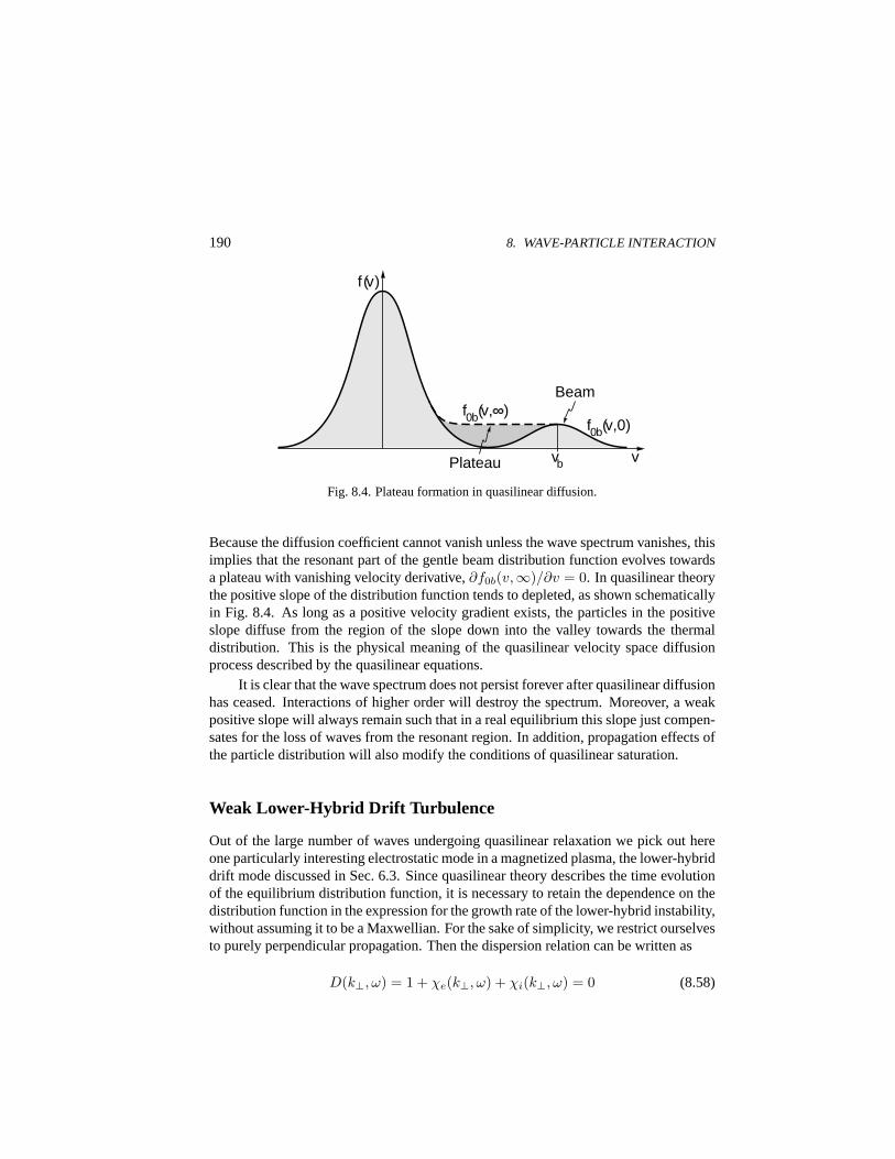
190 8. WAVE-PARTICLE INTERACTION
f (v)
v vb
f0b(v,∞) f0b(v,0)
Beam
Plateau
Fig. 8.4. Plateau formation in quasilinear diffusion.
Because the diffusion coefficient cannot vanish unless the wave spectrum vanishes, thisimplies that the resonant part of the gentle beam distribution function evolves towardsa plateau with vanishing velocity derivative,∂f0b(v,∞)/∂v = 0. In quasilinear theorythe positive slope of the distribution function tends to depleted, as shown schematicallyin Fig. 8.4. As long as a positive velocity gradient exists, the particles in the positiveslope diffuse from the region of the slope down into the valley towards the thermaldistribution. This is the physical meaning of the quasilinear velocity space diffusionprocess described by the quasilinear equations.
It is clear that the wave spectrum does not persist forever after quasilinear diffusionhas ceased. Interactions of higher order will destroy the spectrum. Moreover, a weakpositive slope will always remain such that in a real equilibrium this slope just compen-sates for the loss of waves from the resonant region. In addition, propagation effects ofthe particle distribution will also modify the conditions of quasilinear saturation.
Weak Lower-Hybrid Drift Turbulence
Out of the large number of waves undergoing quasilinear relaxation we pick out hereone particularly interesting electrostatic mode in a magnetized plasma, the lower-hybriddrift mode discussed in Sec. 6.3. Since quasilinear theory describes the time evolutionof the equilibrium distribution function, it is necessary to retain the dependence on thedistribution function in the expression for the growth rate of the lower-hybrid instability,without assuming it to be a Maxwellian. For the sake of simplicity, we restrict ourselvesto purely perpendicular propagation. Then the dispersion relation can be written as
D(k⊥, ω) = 1 + χe(k⊥, ω) + χi(k⊥, ω) = 0 (8.58)
8.3. WEAK PARTICLE TURBULENCE 191
where we introduced the abbreviations
χe(k⊥, ω) =ω2
pe
ω2ge
[1− 1
k⊥Ln
ωge
ω − k⊥vde
]
χi(k⊥, ω) =ω2
pi
k⊥
∫dv⊥
ω − k⊥vde
∂f0i(v⊥, t)∂v⊥
(8.59)
This time it is the ion distribution function which carries the free energy, and thereforethe ion distribution function will evolve quasilinearly in time. The growth rate in thelow drift velocity regime,vde < vthi, is obtained from the linear instability theory andgiven by
γ = − πv2thik
2⊥vde
2|k⊥|(1 + k2⊥/k2
max)2∂f0i
∂v⊥
∣∣∣∣v⊥=ω/k⊥
(8.60)
wherevde = −vdi, andkmax is defined as
k2maxλ
2Di = 2/(1 + ω2
pe/ω2ge) (8.61)
the value of the perpendicular wavenumber where the growth rate maximizes. Hence,quasilinear saturation of lower-hybrid turbulence can proceed in two ways, either bydepleting the resonant part of the distribution function, such that the velocity gradienttends to zero as for Langmuir turbulence, or by reduction of the drift speed,vde → 0.
The evolution of the spectral density follows Eq. (8.50), which we now write as
∂Ww(k⊥, t)/∂t = 2γ(k⊥, t)Ww(k⊥, t) (8.62)
Remembering thatWE(k⊥, t) = ε0|δE(k⊥, t)|2/2 is the electric field energy, and thatthe wave energy contains a contribution from the displacement of the electrons, i.e., acontribution from the polarization of the medium,∂(ωε)/∂ω, we can write the waveenergy as
Ww(k⊥, t) =(1 + ω2
pe/ω2ge
)WE(k⊥, t) (8.63)
The resonantly unstable region covers the range of ion velocities0 < v < vde = vE .In this resonant range the ion velocity evolves according to the quasilinear equation
∂f0i(v, t)∂t
=∂
∂v·[Di(v, t) · ∂f0i(v, t)
∂v
](8.64)
which is the three-dimensional generalization of the electrostatic quasilinear diffusionequation (8.46). Here the diffusion coefficient is defined as
Di(v, t) =2iω2
pi
n0mi
∫d3k
k2
kkWE(k, t)ω(k)− k · v (8.65)
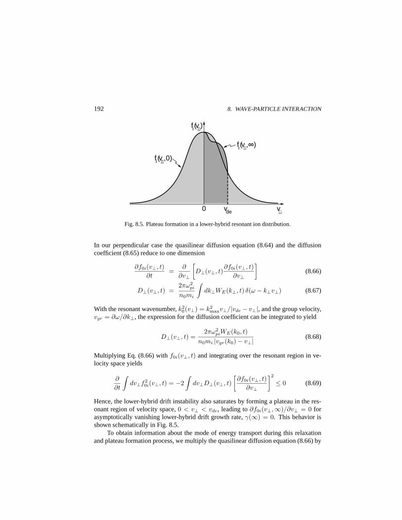
192 8. WAVE-PARTICLE INTERACTION
fi(v⊥)
v⊥ vde 0
fi(v⊥,∞)
fi(v⊥,0)
Fig. 8.5. Plateau formation in a lower-hybrid resonant ion distribution.
In our perpendicular case the quasilinear diffusion equation (8.64) and the diffusioncoefficient (8.65) reduce to one dimension
∂f0i(v⊥, t)∂t
=∂
∂v⊥
[D⊥(v⊥, t)
∂f0i(v⊥, t)∂v⊥
](8.66)
D⊥(v⊥, t) =2πω2
pi
n0mi
∫dk⊥WE(k⊥, t) δ(ω − k⊥v⊥) (8.67)
With the resonant wavenumber,k20(v⊥) = k2
maxv⊥/|vde − v⊥|, and the group velocity,vgr = ∂ω/∂k⊥, the expression for the diffusion coefficient can be integrated to yield
D⊥(v⊥, t) =2πω2
piWE(k0, t)n0mi |vgr(k0)− v⊥| (8.68)
Multiplying Eq. (8.66) withf0i(v⊥, t) and integrating over the resonant region in ve-locity space yields
∂
∂t
∫dv⊥f2
0i(v⊥, t) = −2∫
dv⊥D⊥(v⊥, t)[∂f0i(v⊥, t)
∂v⊥
]2
≤ 0 (8.69)
Hence, the lower-hybrid drift instability also saturates by forming a plateau in the res-onant region of velocity space,0 < v⊥ < vde, leading to∂f0i(v⊥,∞)/∂v⊥ = 0 forasymptotically vanishing lower-hybrid drift growth rate,γ(∞) = 0. This behavior isshown schematically in Fig. 8.5.
To obtain information about the mode of energy transport during this relaxationand plateau formation process, we multiply the quasilinear diffusion equation (8.66) by
8.3. WEAK PARTICLE TURBULENCE 193
v2⊥ and integrate. Inserting the diffusion coefficient from Eq. (8.67) and performing the
integration over theδ-function yields
n0mi
2∂
∂t
∫v2⊥f0idv⊥ =
∫2γ(k⊥, t)Ww(k⊥, t)dk⊥ (8.70)
Since∂Ww/∂t = 2γWw from Eq. (8.62), this equation becomes a conservation lawcontaining the resonant ion kinetic energy density,Wires = (n0mi/2)
∫dv⊥v2
⊥f0i
∂(Wires −Ww)/∂t = 0 (8.71)
Thus the quasilinear saturation level can be estimated by calculating the final resonantparticle kinetic energy level in the plateau region. Fig. 8.5 shows that there is a par-ticular velocity,v∗, inside the resonant region, for which during plateau formation thenumber of particles is conserved. This implies that the value of the distribution func-tion atv⊥ = v∗ is unchanged for all times, and in particularf0i(v∗, 0) = f0i(v∗,∞).Assuming that the initial distribution is a Maxwellian,f0i,m, we get
vdef0i,m(v∗) =∫ vde
0
dv⊥f0i,m(v⊥) (8.72)
Forv2de ¿ v2
thi this equation simply yieldsv∗ = vde/√
3. Calculating for this low driftvelocity regime the net energy change
∆Wires = Wires(∞)−Wires(0) ≈ 0.05 n0kBTi (vde/vthi)5 (8.73)
we find that it goes as the fifth power of the drift-to-thermal velocity ratio. Since thetotal energy is conserved, this is also the change in wave energy between initial andsaturated state,∆Ww. Since the initial wave energy is at the thermal fluctuation leveland can be neglected, we can integrate the wave spectral energy,Ww(k⊥), from Eq.(8.63), over the wavenumber space and obtain the wave energy
(1 +
ω2pe
ω2ge
) ∫dk⊥
(1 +
k2⊥
k2max
)WE(k⊥,∞) = ∆Wires (8.74)
which can be used to estimate the saturated electric field fluctuation level,WE(k⊥,∞).This becomes particularly easy when one assumes that the spectrum is peaked at themaximum wavenumber. Then the bracket containing the ratio of wavenumber to maxi-mum wavenumber under the integral becomes 2, and one finds that
WE(k⊥,∞) = 0.1mi
me
(vde
vthi
)3
Weq (8.75)
194 8. WAVE-PARTICLE INTERACTION
The quantityWeq introduced here is the electric field fluctuation level, which is obtainedwhen the final state can be characterized by equipartition between the kinetic energy andthe wave energy. In this final state one half of the energy is in the waves
Weq =n0mev
2de
8(1 + ω2pe/ω2
ge)(8.76)
This would be the predicted saturation level if current relaxation instead of quasilinearplateau formation would be the mechanism which saturates the lower-hybrid drift in-stability. Equipartition of particle and wave energy is frequently assumed in situationswhere the saturation mechanism is unknown. However, the equipartition saturationlevel may differ strongly from the quasilinearly reached saturation level.
The quasilinear theory gives the possibility to estimate the quasilinear relaxationtime of the ion distribution function until plateau formation is nearly completed. Thisasymptotic time interval, taken to be infinite in the above calculation, is a long but finitetime span, given approximately by the ratio of the square of the ion thermal velocity tothe quasilinear diffusion coefficient
τql ≈ v2thi/2D⊥ (8.77)
To order of magnitude, we can estimate the quasilinear diffusion coefficient
D⊥ ≈ 4π
n0mi
ω2pi
kmaxvdeWE (8.78)
where we used the maximum growing wavenumber andv = vde/2. Since we alreadyknow the saturation level, the quasilinear relaxation time is estimated to
τql ≈ kmaxvde
4πω2pi
n0kBTi
WE(8.79)
Hence, knowing the spectral energy of the electric fluctuations in the lower-hybrid driftinstability, one can estimate the relaxation time. Using the above expressions and theexpression for the maximum linear growth rate,γmax = ωlh(
√2π/8)(v2
de/v2thi), one
findsτqlγmax ≈ 1.4(vthi/vde)2 (8.80)
For completeness we investigate the behavior of the non-resonant ions and electrons.Both are described by the same quasilinear equation, but with the non-resonant part ofthe diffusion coefficient, i.e., the principal-value part and not theδ-function resonantpart. Formally this equation can be written for the ions as
∂F0i
∂t=
∂
∂v⊥
[Dnr(v⊥, t)
∂F0i
∂v⊥
](8.81)
8.3. WEAK PARTICLE TURBULENCE 195
where we used a capitalF to distinguish the non-resonant from the resonant distribu-tion functions, and the non-resonant diffusion coefficient is obtained assuming that thefrequency is low enough to allow to write
Dnr(v⊥, t) =2ω2
pi
min0
∫dk⊥
γ(k⊥, t)WE(k⊥, t)k2⊥v2
⊥(8.82)
With the help of this equation the energy conservation assumes the form
n0mi
2∂
∂t
∫v2⊥dv⊥F0i = −2ω2
pi
∫dk⊥k2⊥
γWE
∫dv⊥v⊥
∂F0i
∂v⊥(8.83)
Because in the non-resonant region the distribution function remains approximatelyunchanged, it can be replaced by a Maxwellian on the right-hand side. After carryingout the differentiation this removes the singularity and produces
∂
∂t
[Wi,nr − 2
∫dk⊥
k2⊥λ2
Di
WE(k⊥, t)]
= 0 (8.84)
whereWi,nr = (n0mi/2)∫
v2⊥dv⊥F0i is the non-resonant kinetic ion energy and the
spectral field energy is replaced by its time variation,2γWE = ∂WE/∂t. At maximumgrowth rate we havek2
⊥ = k2max, and thek⊥-integral over the spectral density gives the
total energy density of the wave field,WE = 2(1 + ω2pe/ω2
ge)∫
dk⊥WE(k⊥) and thus
∂(Wi,nr − 12Ww)/∂t = 0 (8.85)
The non-resonant ion interaction is thus non-negligible in the total energy budget. Thissmall distortion of the non-resonant bulk distribution is best accounted for as a non-resonant heating effect of the bulk ion plasma by the non-resonant absorption of thelower-hybrid wave energy. We can estimate this kind of heating from the last equation,by defining the relative increase in the ion temperature as
∆Ti
Ti=
∆Ww
n0kBTi≈ 2
(1 +
ω2pe
ω2ge
)Weq
n0kBTi(8.86)
or using the wave saturation level
∆Ti/Ti ≈ 0.05(vde/vthi)5 ¿ 1 (8.87)
which in the slow drift limit used here is small. Therefore the bulk plasma heating bythe lower-hybrid drift instability is only weak.
However, the equivalent investigation for electrons shows that electron heating canbe quite substantial. In response to the lower-hybrid drift instability the electrons gainenergy as described by
n0me
2∂
∂t
∫dv⊥(v⊥ − vde)2f0e(v⊥, t) =
ω2pe
ω2ge
∂WE
∂t(8.88)
196 8. WAVE-PARTICLE INTERACTION
Thus the heating rate of the electrons is quite substantial if the plasma-to-cyclotronfrequency ratio is large. The electrons gain heat at a very fast rate, faster than thewave fluctuations grow. But the heating of the bulk of the electrons still remains small.Energy is only fed to the few resonant electrons which are accelerated in the wave field.
Weak Whistler Turbulence
We now turn to electromagnetic waves below the electron-cyclotron frequency. Forsimplicity we consider only parallel propagation of the R- and L-modes (see Sec. 10.6of our companion book). The linear distortion of the distribution function caused bythese waves is given in Eq. (I.10.91) in terms of the initial non-equilibrium distribution,f0s. For parallel propagation, performing the integration over the gyrating particle orbit,we get for the linear disturbance
δfsR,L(k,v, t) = − iqs
2ms
δER,L(k, t)ω(k, t)− kv‖ ± ωgs[
1− kv‖ω(k, t)
]∂
∂v⊥+
kv⊥ω(k, t)
∂
∂v‖
f0s(v⊥, v‖, t) (8.89)
wherek = k‖ is the parallel wavenumber, and we have indicated explicitly the depen-dence on wavenumber and time in the frequency,ω, and in the undisturbed backgrounddistribution, f0s(t). The time dependence in the frequency leads to the time evolu-tion of the growth rate,γ(k, t), which we again expect to vanish asymptotically in thelong-time limit, when the quasilinear stable state is reached. This growth rate mustbe positive,γ(k, t) > 0, because otherwise the wave field dies out and there is no re-markable distortion of the distribution function. Growing whistlers and electromagneticion-cyclotron waves are obtained, for instance, for an excess temperature in the perpen-dicular direction,As > 0. But there are also other possibilities to drive these wavesunstable, such as loss cones and beams.
The linear growth rate is determined from the linear dispersion relation, which foran unspecified distribution function is given as
DR,L = 1− k2c2
ω2(k, t)+
∑s
ω2ps
2ω2(k, t)
∫d3v
v⊥ω(k, t)− kv‖ ∓ ωgs
·[
1− kv‖ω(k, t)
]∂
∂v⊥+
kv⊥ω(k, t)
∂
∂v‖
f0s(v⊥, v‖, t) = 0 (8.90)
Finding the quasilinear equation of weak turbulence in even this simple case of par-allel propagation requires quite some algebra. The steps of the calculation are as fol-lows. Take the quasilinear equation (8.38) and write it for parallel propagation and agyrotropic undisturbed distribution function, which does not depend on the gyration
8.3. WEAK PARTICLE TURBULENCE 197
angle,φ, of the particles. Then replace the wave fields on the right-hand side in theensemble-averaged part by the right- and left-polarized electromagnetic fields
δER,L(k, t) = δEx(k, t)∓ iδEy(k, t) (8.91)
thereby expressing the magnetic through the electric wave field using Maxwell’s secondequation. Now expand the wave field and the disturbance of the distribution on theright-hand side into Fourier series both in space and time, using differentk andω in thetwo Fourier integrals. At this point insertδf from Eq. (8.89) to express the right-handside in terms of the electric wave field and the background distribution function only.
The next step is to interpret the average as integrals over the fast space-time vari-ation of the wave field, keeping the background distribution and frequency constantand assuming that averages over linear quantities vanish in the random-phase approx-imation. Performing this integration over all space and time reduces the two Fourierintegrals to just one, because the random-phase approximation producesδ-functions ofthe typeδ(ω − ω1 − ω2)δ(k − k1 − k2). Remembering that the wave fields are real,δE(k, ω)δE(−k,−ω) = |δE(k, ω)|2, we define
ε0⟨|δE(k, t)|2⟩ = 2WE(k, t) (8.92)
where the time dependence refers to the slow variation of the averages only, since fasttime variations have been averaged out. Finally, we average over the gyration angle,ψ,from 0 to 2π using that due to gyrotropy of the initial background distribution
12π
∫ 2π
0
dψ∂f0s
∂ψ= 0 (8.93)
which shows that the final average distribution is also gyrotropic, despite the presenceof the waves and their modifying effect. We then obtain
∂f0s
∂t=
iω2ps
2msns
∑±
∫dkWE(k, t)
[1 +
kv‖ω(−k, t)
]1v⊥
∂
∂v⊥
− kv⊥ω(−k, t)
∂
∂v‖
1
ω(k, t)− kv‖ ± ωgs
1− kv‖
ω(k, t)∂
∂v⊥+
kv⊥ω(k, t)
∂
∂v‖
f0s
(8.94)
for the general parallel kinetic equation of weak electromagnetic plasma turbulencetheory. The sum in this equation is over the two resonant contributions, correspondingto the two directions of propagation parallel and antiparallel to the magnetic field,±k.
The complicated expression on the right-hand side, in front of the slowly varyingbackground distribution function, is the velocity space diffusion term. Obviously, in themagnetized plasma it depends on the two velocity derivatives parallel and perpendicular
198 8. WAVE-PARTICLE INTERACTION
to the magnetic field. The important conclusion drawn from the above quasilinear weakturbulence kinetic equation (8.94) is that the background resonant distribution functionexperiences a two-dimensional velocity space diffusion inv‖ andv⊥ under the actionof the parallel propagating electromagnetic R- and L-modes, while the evolution of thewave spectral density in this theory follows Eq. (8.50)
∂WE(k, t)/∂t = 2γ(k, t)WE(k, t) (8.95)
We will now apply the present theory to whistlers excited by a temperature anisotropy,under the assumption that|ω(k) − ωge| À kvthe and|γ(k)/ω(k)| ¿ 1. The growthrate of the whistler, expressed through the initial undisturbed distribution is
γ(k, t) =π
2ω(k)ω2
pe
∫d3v
v⊥δ(ω − kv‖ − ωge)ω2 + c2k2 + ω2ω2
pe/(ω − ωge)2
·[(ω − kv‖)
∂
∂v⊥+ kv⊥
∂
∂v‖
]f0e (8.96)
Taking into account only resonant interactions leads to the replacement of the denomi-nator by theδ-function. The same replacement must be used also in the diffusion termof Eq. (8.94), which becomes
∂f0e(t)∂t
=πω2
pe
2men0
∫
k≥0
dkWE(k, t)[(
1− kv‖ω
)1v⊥
∂
∂v⊥v⊥ +
kv⊥ω
∂
∂v‖
]
δ(kv‖ − ω + ωge)[(
1− kv‖ω
)∂
∂v⊥+
kv⊥ω
∂
∂v‖
]f0e(t) (8.97)
whereω(k) is the whistler frequency, given as the solution of the real part of the disper-sion relation in Eq. (5.10). The kinetic equation (8.97) describes the nonlinear evolutionof the resonant part of the unstable electron distribution function. As for the Langmuirand lower-hybrid waves, we multiply Eq. (8.97) by the distribution function,f0e, andintegrate over the resonant part of the phase space to find
d
dt
∫d3vf2
0e(t) = − πω2pe
men0
∫dk
ω(k)WE(k, t)
∫d3v δ(kv‖ − ω + ωge)
·[(ω − kv‖)
∂f0e
∂v⊥+ kv⊥
∂f0e
∂v‖
]2
≤ 0 (8.98)
The right-hand side is always negative. Hence, the evolution of the resonant part of thedistribution function tends towards an equilibrium, where the expression in the bracketsvanishes for all resonant velocities
vres = [ω(k)− ωge]/k (8.99)
8.4. RESONANCE BROADENING 199
In the long-time asymptotic limit this bracket must vanish, simply because the trivialpossibility that the wave spectral density becomes zero makes sense only for dampedwaves, in which case the quasilinear theory is of no interest. One thus requires as thefinal state of the distribution function in the resonant interval of phase space
kv⊥∂f0e(∞)/∂v‖|v‖=vres+ (ω − kv‖)∂f0e(∞)/∂v⊥|v‖=vres
= 0 (8.100)
This condition is equivalent to the requirement that in the final state of quasilinearevolution of the whistler turbulence the linear growth rate has turned zero,γ(∞) = 0.
In order to determine what this conclusion implies for the evolution of the distri-bution function in the resonant phase space interval, we observe that Eq. (8.100) hasthe characteristic differential equation
dv‖/dv⊥ = v⊥/[(ω/k)− v‖] (8.101)
whereω(k)/k must be taken at the resonant velocity (8.99). Integration yields that
v2⊥ + v2
‖
2−
∫ vres
0
dv‖ω(v‖)
k= const (8.102)
is a constant of motion of the particles in the resonant region in the whistler wave fieldin the final state. Hence, the final resonant velocity distribution is given by
f0e(v⊥, v‖,∞) = f0e
[v2‖ + v2
⊥2
−∫ vres
0
dv‖ω(v‖)
k
](8.103)
We know, however, that the resonant strip in(v⊥, v‖)-space is centered at the nega-tive wave phase velocityv‖ = −(ω/k) but otherwise parallel to thev⊥-axis (see theunstable right-hand part of Fig. 5.2). This strip has the coordinates
[ω(k1)− ωge]/k1 < v‖ < [ω(k2)− ωge]/k2 (8.104)
and0 < v⊥ < ∞. The curves where the argument of the asymptotically stable resonantelectron distribution function is constant are the sections of the circles in(v⊥, v‖)-spacecentered atv‖ = −(ω/k), v⊥ = 0. During quasilinear evolution the distribution evolvesin phase space along these stable orbits.
8.4. Resonance Broadening
In the derivation of quasilinear wave-particle interaction we have continuously assumedthat the orbits of the particles remain undisturbed by the wave field. This assumptionholds for very weak wave fields. However, when the wave grows to large amplitudes,
200 8. WAVE-PARTICLE INTERACTION
the orbits of the particles may become distorted. Particle trapping in the wave is one ofthe possible effects. In a broad random-phase wave spectrum this trapping is not veryimportant, but distortion of the particle orbits will nevertheless occur. In such a case onecannot consider these orbits as unperturbed, but must include the average wave field incalculating the particle orbits. This is a very involved task. It is considerably simplerto assume that the distortion of the particle orbits produces a shift in the resonant wavefrequencies and thus causesresonance broadeningin a wide wave spectrum containinga large number of harmonics. Resonance broadening leads to leakage of particles outof the resonance and is thus it is another important mechanism of wave saturation andstabilization of instabilities.
Mechanism
The equation for the linear variation of the distribution function in random phase inter-action between particles and waves can be written
[i(k · v − ω)− ∂
∂v·(
D∂
∂v
)]δfs(k) = − qs
msδE(k) · ∂f0s
∂v(8.105)
where, for purely electrostatic variations withδE||k, the diffusion coefficient,D, is
D = −Reiq2
s
m2s
∑
k′
k′k′
k′2|δE(k′)|2
(k′ + k) · v − (ω′ + ω)(8.106)
That the equation forδf already contains a term which depends on the diffusion coef-ficient of the plasma in the wave field, arises from the interaction of the particles withtheir distorted orbits with the broadband wave field and is a deviation from linear theory.
When operating with this new expression forδf and building the modified quasi-linear equations, one arrives at a quasilinear diffusion equation which contains the dif-fusion coefficient in a much more complicated version. To demonstrate this behaviorlet us, for the sake of simplicity, restrict ourselves to one dimension only. In additionwe assume that the diffusion coefficient is constant. Then Eq. (8.105) simplifies to
i(kv − ω)δfs(k)−D∂2δfs(k)
∂v2= − qs
msδE(k)
∂f0s
∂v(8.107)
Fourier-transforming the disturbed distribution function in velocity space
δf(k, v) =12π
∫δf(τ) exp(ivτ)dτ (8.108)
yields for the Fourier-transform,δf(τ) =∫
δf(k, v) exp(−ivτ)dv
dδfs(τ)dτ
+(
iω
k− τ2
kD
)δfs(τ) =
qs
ms
δE(k)k
∫∂f0s
∂vexp(−ivτ)dv (8.109)
8.4. RESONANCE BROADENING 201
The solution of this equation is obtained by direct integration. The result is
δfs(τ) =qsδE(k)
mskexp
[− (iωτ/k −Dτ3/3k
)] ∫ τ
−∞dτ ′
exp
[− (iωτ ′/k −Dτ ′3/3k
)] ∫dv′
∂f0s
∂vexp(−iv′τ ′)
(8.110)
This shows the exponential dependence of the disturbed distribution function on thediffusion coefficient,D, destroying the delta-function character of the resonance. Wedefine the velocity half-width of the particle resonance asδ ≈ k−1(k2D/3)1/3, solvethe Fourier integral overτ , and interpret the result as a resonant denominator
δfs(k) ≈ − iqs
ms
δE(k)ω − kv + ikδ
∂f0s
∂v(8.111)
The distortion of the particle orbits introduces an additional term into the resonant de-nominator inδfs, which causes the broadening of the resonance during the interactionbetween waves and particles. The resonance diffuses until the instability saturates.
Ion-Acoustic Mode
In particular, for resonant excitation of ion-acoustic waves by hot field-aligned electroncurrents and cold ions (see Sec. 4.2), the resonance broadening appear on the electronsonly. In this case the imaginary part of the dielectric constant, including the resonancebroadeningδ = (k2D/3)1/3, is proportional to
Im ε ∝∫
dv (∂f0e/∂v) δ
[ω − k(v0 + u)]2 + δ2(8.112)
wherev0 is the current speed, andu is the width of the resonance. For large resonancebroadening,δ À kv0, the integral tends to zero as1/δ. This implies a vanishinggrowth rate and thus saturation. The instability considered is resonant in the intervalcia < v0 < vthe. Thus stabilization is achieved when the resonance broadens beyondthis domain. This happens when the resonant width,∆ω, approaches the value
∆ω = kvthe = (k2D/3)1/3 (8.113)
Using the bandwidth,∆k, the diffusion coefficient can be expressed as
D ≈(
mi
me
)1/2 πω2pe
∆kvthe
WE
n0kBTev2the (8.114)
202 8. WAVE-PARTICLE INTERACTION
This enables us to determine the saturation level of the ion-acoustic instability, when-ever the saturation is provided by simple resonance broadening in the turbulent wavefield
WE,ia
n0kBTe≈
(me
mi
)1/2
kλD (8.115)
This saturation level is surprisingly low. It indicates that the distortion of the electronorbits in the wave field of the current-driven ion-acoustic wave is very strong. Theparticle orbits are readily deformed, resonance broadening sets on, and the instabilitysaturates on the low level given by Eq. (8.115).
Ion-Cyclotron Resonance Broadening
Another important case is the excitation of electrostatic ion-cyclotron waves by field-aligned currents which has been discussed in Sec. 4.4. This case includes the effects ofthe magnetic field on the particle motion and is considerably more involved than reso-nance broadening in ion-acoustic waves. We write the dielectric response susceptibilityof speciess including the resonance broadening in the denominator
χs(k, ω) =1
k2λ2Ds
[1− (ω − k‖vds)
∞∑
l=−∞
∫d3v fs(v)
J2l (k⊥v⊥/ωgs)
ω + i∆ωs(v)− k‖v‖ − lωgs
]
(8.116)The resonance broadening in frequency symbolized by the imaginary frequency termin the denominator contains of course the full magnetized diffusion tensor. But fork‖/k ¿ 1 the resonance broadening is predominantly transverse to the magnetic field.Resonance broadening is now due to the ions because at these low frequencies theelectrons behave adiabatically. Restricting toD⊥ only, it can be estimated to
k2⊥D⊥ ≈
(k⊥δE
B0
)2 ∆ωiG(k⊥v⊥/ωgi)(ω − k‖v‖ − ωgi)2 + ∆ω2
i
(8.117)
where we used only the first harmonic,l=1, neglected electrons, and introduced
G(ζi) = 14
[J2
0 (ζi) + 2J21 (ζi) + J2
2 (ζi)]
(8.118)
Saturation occurs for∆ωi = k2⊥D⊥, a condition which yields for the ion-cyclotron
mode the wave amplitude at saturation
eδEsat
k⊥kBTe≈ ω2
giΛ1(k2⊥v2
thi/ω2gi)
k2⊥v2
thi[G(21/2k⊥vthi/ωgi)]1/2(8.119)
Here we used the functionΛl(ζ) = Il(ζ) exp(−ζ). This saturation amplitude is inde-pendent of the growth rate which at saturation is zero, and the above result is valid as
8.5. PITCH ANGLE DIFFUSION 203
long as the linear growth rate satisfies the conditionγ/(ω − ωgi) ¿ 1. This saturationamplitude of current driven electrostatic ion cyclotron waves plays an important rolein the calculation of anomalous collision frequencies in ion-cyclotron turbulence, forresonance broadening is the main saturation mechanism in this type of waves.
8.5. Pitch Angle Diffusion
The quasilinear theory developed in the last section can be applied to the particle dy-namics in the magnetosphere. One must, however, distinguish between energetic parti-cles and particles of lower energy. Energetic particles interact better with electromag-netic waves, simply because their energy may exceed the threshold resonance energyfor this kind of interaction. The low energy component requires a different mechanism.
Whistler Turbulence
Assume that an energetic electron component is trapped in the dipolar geomagneticfield close to the Earth, performing bounce motions along the magnetic field betweenthe mirror points of the particles, and at the same time gyrating about the geomagneticfield. Electrons having their mirror point in the deep ionosphere will be lost from themagnetic mirror due to collisions with the neutrals and the dense ionospheric plasma.Therefore the energetic particle distribution function of the trapped electrons will be aloss cone distribution. The trapped electrons will thus have some kind of temperatureanisotropy,Aeh > 0. In addition, the radiation belts are at comparably low geomagneticlatitudes inside the dense plasmasphere withn0 À neh.
Under these conditions, for sufficiently large trapped radiation belt electron fluxes,the hot electron component will excite whistler wave turbulence at frequencies belowthe threshold frequency,ω < ωc, where
ωc/ωge = Aeh/(Aeh + 1) (8.120)
The growth rate of these waves is proportional to the ratio of trapped-to-plasmasphericelectrons,neh/n0, and the whistlers propagate on the background plasmaspheric plasma.The whistler waves, being trapped in the geomagnetic field and bouncing in space be-tween the lower-hybrid resonance points, readily reach large amplitudes, thereby enter-ing the quasilinear regime. They start scattering the electrons and building up a platformin the resonant velocity space. Intuitively the only way to deplete the resonant electronsis to scatter them into the loss cone. This mechanism explains in a simple and satis-factory way the enhanced precipitation of electrons from the radiation belts in all caseswhen the flux of electrons in the radiation belts is enhanced, e.g., during substormswhen transversely accelerated energetic electrons are injected into the radiation beltsfrom the Earth’s tail.
204 8. WAVE-PARTICLE INTERACTION
Consider the distribution function in the quasilinear limit given in Eq. (8.103). Inthis readily reached final stage the change in total energy of an electron,We, associatedwith the change in the parallel energy,We‖, is given by
dWe
dWe‖=
ω
kv‖=
ω
ω − ωc(8.121)
As a consequence, one expects that the particle energy is nearly unchanged for fre-quencies sufficiently far below the critical frequency. At such frequencies, which arehighly plausible because their resonant particle energy is lowest, the diffusion causedby the interaction of the electron distribution and the whistlers is apitch angle diffusion,turning the particle orbits into the loss cone. The quasilinear diffusion equation for theelectrons then becomes a pure pitch angle diffusion equation
∂f0e(v, α, t)∂t
=1
sin α
∂
∂α
[D(v, α, t) sin α
∂f0e(v, α, t)∂α
](8.122)
whereα = tan−1(v‖/v⊥) is the pitch angle of a particle with velocityv and the diffu-sion coefficient for constant energy, rewritten in terms of the magnetic fluctuation fieldcomponent instead of the electric field, is given by
D(v, α, t) = π2ω2c
∑
k
1|k‖|
∣∣∣∣δB(k)
B0
∣∣∣∣2
δ
(v cos α− ω − ωc
k‖
)(8.123)
In order to describe the stationary state achieved in equilibrium between injection andprecipitation, it is convenient to assume that the particles are injected in the nightsideequatorial plane with pitch angles outside the equatorial loss cone angle,α > α`. Withan injection source,Se(v, α), the stationary diffusion equation becomes
1sinα
∂
∂α
[D(v, α) sin α
∂f0e(v, α)∂α
]= Se(α, v) (8.124)
Within the loss cone atα < α`, and forα` ¿ 1, the diffusion equation must besupplemented by a loss term which can simply be modeled asf(α, v)/τ`(α, v). Hereτ` is the characteristic loss time of the precipitating particles which is determined bytheir bounce motion along the magnetic field and is for immediate loss equal to onequarter bounce period. This choice allows to write
1α
∂
∂α
[αD(α, v)
∂f(α, v)∂α
]− f(α, v)
τ`(α, v)= 0 (8.125)
These two equations together with the appropriate boundary condition, that the distribu-tion functions and their derivatives be continuous across the boundary of the loss cone
8.5. PITCH ANGLE DIFFUSION 205
atα = α`, and an appropriate expression for the diffusion coefficient describe the pitchangle scattering in a spatially homogeneous radiation belt.
The choice made for the diffusion coefficient depends on the interaction mech-anism between the whistlers and the particles. A simple choice is to assume thatD ≈ D0α
q for small pitch angles inside the loss cone. Integrating Eq. (8.124) twicewith respect toα and defining
〈Se(v)〉 =∫ π/2
α`
dα′ sin α′Se(α′, v) (8.126)
and assuming for simplicity that the injection is atα = π/2 only, such thatSe(v, α′) =S(v)δ(α′ − π/2), the external solution is
fe(α, v) = 〈Se(v)〉[∫ α
α`
dα′′
sin α′′D(α′′)+ h(α`)
](8.127)
The arbitrary function,h(α), has to be determined from the boundary conditions. Theinterior solution may be expressed in terms of modified Bessel functions. DemandingthatD0α
q+1` ∂h/∂α|α`
= 〈S〉, one finds
h(α) =1
D0αq/2
(D0τ`
α2`
)1/2 Iq/(2−q)
[(1− q/2)−1(α2−q/D0τ`)1/2
]
Iq/(2−q)
[(1− q/2)−1(α2−q
` /D0τ`)1/2] (8.128)
Two limiting cases are of interest. The first isweak pitch angle diffusion, when theparticles drift into the loss cone at a much slower rate than they are lost, implying thatthe diffusion time is longer than one quarter bounce period. In this limitD0τ` ¿ 1 and
hwd(α) ≈ 1D0αq/2
(D0τ`
α2`
)1/2(α`
α
)2−q4
exp
(
α2−q
D0τ`
)1/2
−(
α2−q`
D0τ`
)1/2
(8.129)One realizes that this solution contains one special limiting case,q = 2, when thesolution changes character. Forq > 2 the solution decays exponentially from the losscone boundary down toα = 0. Because there are only few particles inside the losscone and few particles per unit time enter it, the particle precipitation is a slow drizzleof particles into the ionosphere. This is the usual weak diffusion precipitation case.Qualitatively this behavior is the same for allq.
The other case of interest is when the diffusion into the loss cone is so strong thatthe particles enter the loss cone in a time comparable to or shorter than the quarterbounce period. ThenD0τ` À 1 and the Bessel functions can then be expanded in thesmall-amplitude limit, yielding
hsd(α) ≈ 2τ`/α2` À 1 (8.130)
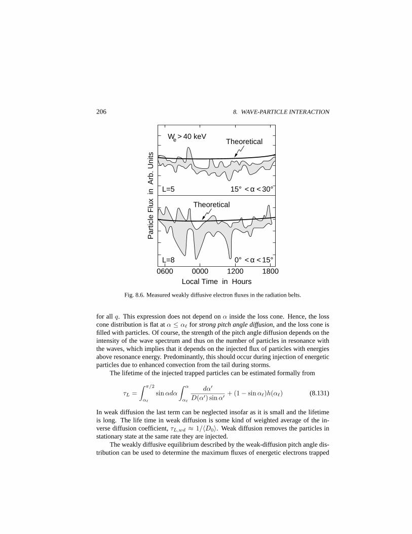
206 8. WAVE-PARTICLE INTERACTION
15° < α < 30°
0° < α < 15° L=8
L=5
Theoretical
0600 0000 1200 1800 Local Time in Hours
Par
ticle
Flu
x in
Arb
. Uni
ts
We > 40 keV Theoretical
Fig. 8.6. Measured weakly diffusive electron fluxes in the radiation belts.
for all q. This expression does not depend onα inside the loss cone. Hence, the losscone distribution is flat atα ≤ α` for strong pitch angle diffusion, and the loss cone isfilled with particles. Of course, the strength of the pitch angle diffusion depends on theintensity of the wave spectrum and thus on the number of particles in resonance withthe waves, which implies that it depends on the injected flux of particles with energiesabove resonance energy. Predominantly, this should occur during injection of energeticparticles due to enhanced convection from the tail during storms.
The lifetime of the injected trapped particles can be estimated formally from
τL =∫ π/2
α`
sin αdα
∫ α
α`
dα′
D(α′) sin α′+ (1− sinα`)h(α`) (8.131)
In weak diffusion the last term can be neglected insofar as it is small and the lifetimeis long. The life time in weak diffusion is some kind of weighted average of the in-verse diffusion coefficient,τL,wd ≈ 1/〈D0〉. Weak diffusion removes the particles instationary state at the same rate they are injected.
The weakly diffusive equilibrium described by the weak-diffusion pitch angle dis-tribution can be used to determine the maximum fluxes of energetic electrons trapped
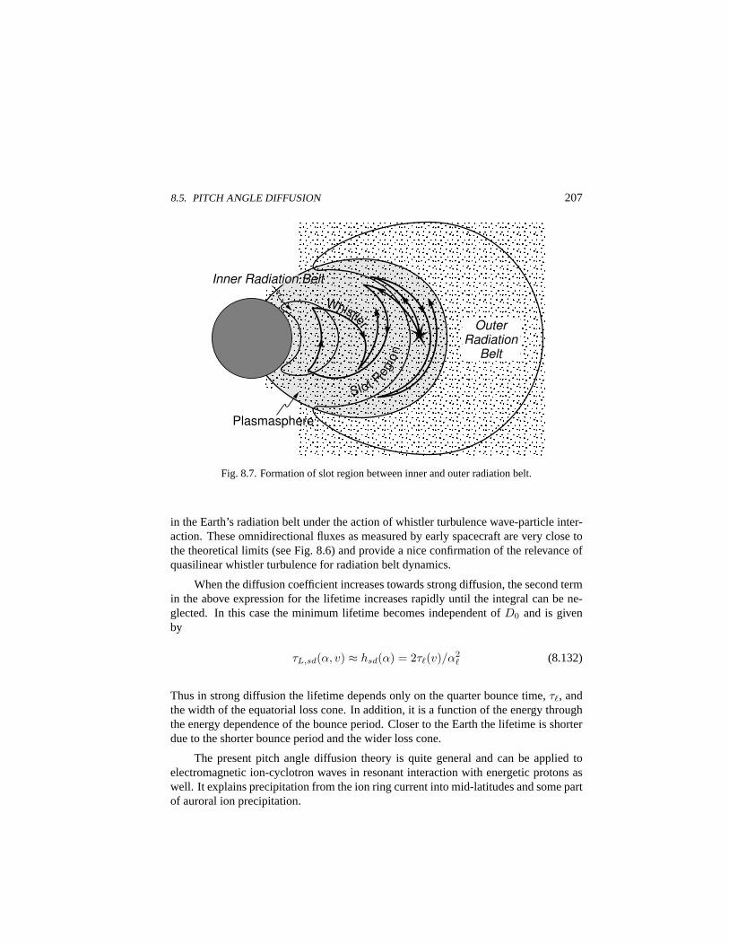
8.5. PITCH ANGLE DIFFUSION 207
Whistler
Slot Regio
n
Inner Radiation Belt
Outer Radiation
Belt
Plasmasphere
Fig. 8.7. Formation of slot region between inner and outer radiation belt.
in the Earth’s radiation belt under the action of whistler turbulence wave-particle inter-action. These omnidirectional fluxes as measured by early spacecraft are very close tothe theoretical limits (see Fig. 8.6) and provide a nice confirmation of the relevance ofquasilinear whistler turbulence for radiation belt dynamics.
When the diffusion coefficient increases towards strong diffusion, the second termin the above expression for the lifetime increases rapidly until the integral can be ne-glected. In this case the minimum lifetime becomes independent ofD0 and is givenby
τL,sd(α, v) ≈ hsd(α) = 2τ`(v)/α2` (8.132)
Thus in strong diffusion the lifetime depends only on the quarter bounce time,τ`, andthe width of the equatorial loss cone. In addition, it is a function of the energy throughthe energy dependence of the bounce period. Closer to the Earth the lifetime is shorterdue to the shorter bounce period and the wider loss cone.
The present pitch angle diffusion theory is quite general and can be applied toelectromagnetic ion-cyclotron waves in resonant interaction with energetic protons aswell. It explains precipitation from the ion ring current into mid-latitudes and some partof auroral ion precipitation.
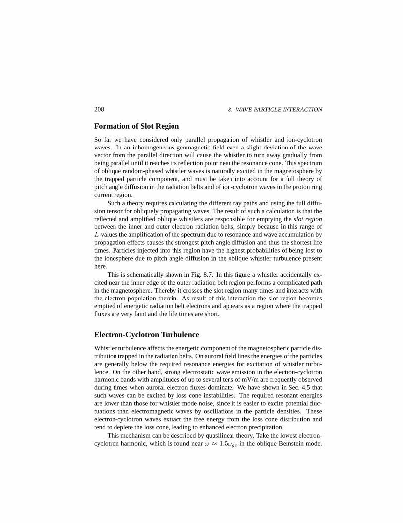
208 8. WAVE-PARTICLE INTERACTION
Formation of Slot Region
So far we have considered only parallel propagation of whistler and ion-cyclotronwaves. In an inhomogeneous geomagnetic field even a slight deviation of the wavevector from the parallel direction will cause the whistler to turn away gradually frombeing parallel until it reaches its reflection point near the resonance cone. This spectrumof oblique random-phased whistler waves is naturally excited in the magnetosphere bythe trapped particle component, and must be taken into account for a full theory ofpitch angle diffusion in the radiation belts and of ion-cyclotron waves in the proton ringcurrent region.
Such a theory requires calculating the different ray paths and using the full diffu-sion tensor for obliquely propagating waves. The result of such a calculation is that thereflected and amplified oblique whistlers are responsible for emptying theslot regionbetween the inner and outer electron radiation belts, simply because in this range ofL-values the amplification of the spectrum due to resonance and wave accumulation bypropagation effects causes the strongest pitch angle diffusion and thus the shortest lifetimes. Particles injected into this region have the highest probabilities of being lost tothe ionosphere due to pitch angle diffusion in the oblique whistler turbulence presenthere.
This is schematically shown in Fig. 8.7. In this figure a whistler accidentally ex-cited near the inner edge of the outer radiation belt region performs a complicated pathin the magnetosphere. Thereby it crosses the slot region many times and interacts withthe electron population therein. As result of this interaction the slot region becomesemptied of energetic radiation belt electrons and appears as a region where the trappedfluxes are very faint and the life times are short.
Electron-Cyclotron Turbulence
Whistler turbulence affects the energetic component of the magnetospheric particle dis-tribution trapped in the radiation belts. On auroral field lines the energies of the particlesare generally below the required resonance energies for excitation of whistler turbu-lence. On the other hand, strong electrostatic wave emission in the electron-cyclotronharmonic bands with amplitudes of up to several tens of mV/m are frequently observedduring times when auroral electron fluxes dominate. We have shown in Sec. 4.5 thatsuch waves can be excited by loss cone instabilities. The required resonant energiesare lower than those for whistler mode noise, since it is easier to excite potential fluc-tuations than electromagnetic waves by oscillations in the particle densities. Theseelectron-cyclotron waves extract the free energy from the loss cone distribution andtend to deplete the loss cone, leading to enhanced electron precipitation.
This mechanism can be described by quasilinear theory. Take the lowest electron-cyclotron harmonic, which is found nearω ≈ 1.5ωge in the oblique Bernstein mode.
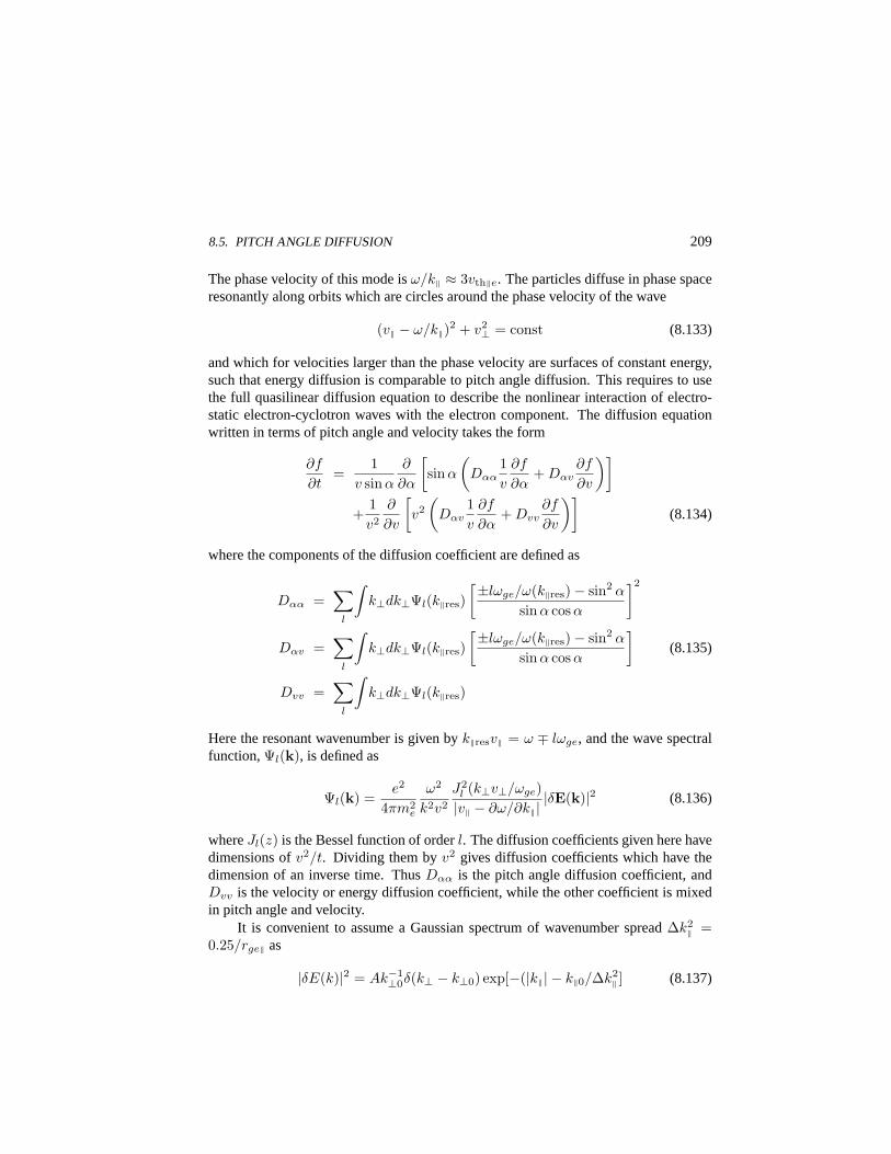
8.5. PITCH ANGLE DIFFUSION 209
The phase velocity of this mode isω/k‖ ≈ 3vth‖e. The particles diffuse in phase spaceresonantly along orbits which are circles around the phase velocity of the wave
(v‖ − ω/k‖)2 + v2⊥ = const (8.133)
and which for velocities larger than the phase velocity are surfaces of constant energy,such that energy diffusion is comparable to pitch angle diffusion. This requires to usethe full quasilinear diffusion equation to describe the nonlinear interaction of electro-static electron-cyclotron waves with the electron component. The diffusion equationwritten in terms of pitch angle and velocity takes the form
∂f
∂t=
1v sinα
∂
∂α
[sin α
(Dαα
1v
∂f
∂α+ Dαv
∂f
∂v
)]
+1v2
∂
∂v
[v2
(Dαv
1v
∂f
∂α+ Dvv
∂f
∂v
)](8.134)
where the components of the diffusion coefficient are defined as
Dαα =∑
l
∫k⊥dk⊥Ψl(k‖res)
[±lωge/ω(k‖res)− sin2 α
sin α cosα
]2
Dαv =∑
l
∫k⊥dk⊥Ψl(k‖res)
[±lωge/ω(k‖res)− sin2 α
sin α cosα
](8.135)
Dvv =∑
l
∫k⊥dk⊥Ψl(k‖res)
Here the resonant wavenumber is given byk‖resv‖ = ω ∓ lωge, and the wave spectralfunction,Ψl(k), is defined as
Ψl(k) =e2
4πm2e
ω2
k2v2
J2l (k⊥v⊥/ωge)|v‖ − ∂ω/∂k‖| |δE(k)|2 (8.136)
whereJl(z) is the Bessel function of orderl. The diffusion coefficients given here havedimensions ofv2/t. Dividing them byv2 gives diffusion coefficients which have thedimension of an inverse time. ThusDαα is the pitch angle diffusion coefficient, andDvv is the velocity or energy diffusion coefficient, while the other coefficient is mixedin pitch angle and velocity.
It is convenient to assume a Gaussian spectrum of wavenumber spread∆k2‖ =
0.25/rge‖ as
|δE(k)|2 = Ak−1⊥0δ(k⊥ − k⊥0) exp[−(|k‖| − k‖0/∆k2
‖ ] (8.137)
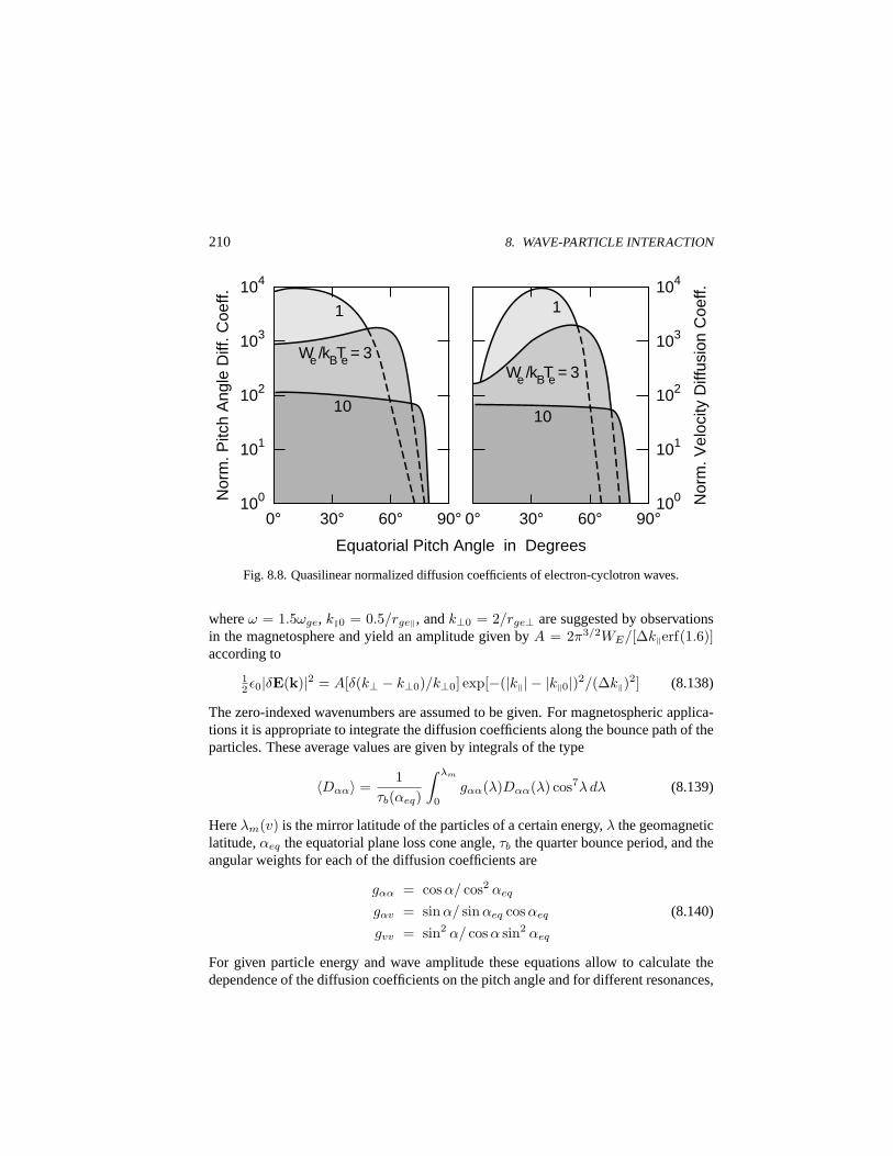
210 8. WAVE-PARTICLE INTERACTION
0° 30° 60° 90° 100
101
102
103
104
0° 30° 60° 90° 100
101
102
103
104
Equatorial Pitch Angle in Degrees
Nor
m. P
itch
Ang
le D
iff. C
oeff.
Nor
m. V
eloc
ity D
iffus
ion
Coe
ff.
1
10 10
1
We /kBTe = 3 We /kBTe = 3
Fig. 8.8. Quasilinear normalized diffusion coefficients of electron-cyclotron waves.
whereω = 1.5ωge, k‖0 = 0.5/rge‖, andk⊥0 = 2/rge⊥ are suggested by observationsin the magnetosphere and yield an amplitude given byA = 2π3/2WE/[∆k‖erf(1.6)]according to
12ε0|δE(k)|2 = A[δ(k⊥ − k⊥0)/k⊥0] exp[−(|k‖| − |k‖0|)2/(∆k‖)2] (8.138)
The zero-indexed wavenumbers are assumed to be given. For magnetospheric applica-tions it is appropriate to integrate the diffusion coefficients along the bounce path of theparticles. These average values are given by integrals of the type
〈Dαα〉 =1
τb(αeq)
∫ λm
0
gαα(λ)Dαα(λ) cos7λ dλ (8.139)
Hereλm(v) is the mirror latitude of the particles of a certain energy,λ the geomagneticlatitude,αeq the equatorial plane loss cone angle,τb the quarter bounce period, and theangular weights for each of the diffusion coefficients are
gαα = cos α/ cos2 αeq
gαv = sinα/ sin αeq cosαeq (8.140)
gvv = sin2 α/ cosα sin2 αeq
For given particle energy and wave amplitude these equations allow to calculate thedependence of the diffusion coefficients on the pitch angle and for different resonances,
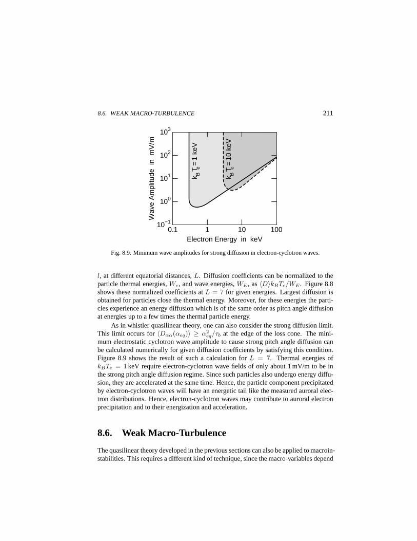
8.6. WEAK MACRO-TURBULENCE 211
10−1
100
101
102
103
0.1 1 10 100 Electron Energy in keV
Wav
e A
mpl
itude
in
mV
/m
k BT e
=1
keV
k BT e
=10
keV
Fig. 8.9. Minimum wave amplitudes for strong diffusion in electron-cyclotron waves.
l, at different equatorial distances,L. Diffusion coefficients can be normalized to theparticle thermal energies,We, and wave energies,WE , as〈D〉kBTe/WE . Figure 8.8shows these normalized coefficients atL = 7 for given energies. Largest diffusion isobtained for particles close the thermal energy. Moreover, for these energies the parti-cles experience an energy diffusion which is of the same order as pitch angle diffusionat energies up to a few times the thermal particle energy.
As in whistler quasilinear theory, one can also consider the strong diffusion limit.This limit occurs for〈Dαα(αeq)〉 ≥ α2
eq/τb at the edge of the loss cone. The mini-mum electrostatic cyclotron wave amplitude to cause strong pitch angle diffusion canbe calculated numerically for given diffusion coefficients by satisfying this condition.Figure 8.9 shows the result of such a calculation forL = 7. Thermal energies ofkBTe = 1 keV require electron-cyclotron wave fields of only about 1 mV/m to be inthe strong pitch angle diffusion regime. Since such particles also undergo energy diffu-sion, they are accelerated at the same time. Hence, the particle component precipitatedby electron-cyclotron waves will have an energetic tail like the measured auroral elec-tron distributions. Hence, electron-cyclotron waves may contribute to auroral electronprecipitation and to their energization and acceleration.
8.6. Weak Macro-Turbulence
The quasilinear theory developed in the previous sections can also be applied to macroin-stabilities. This requires a different kind of technique, since the macro-variables depend
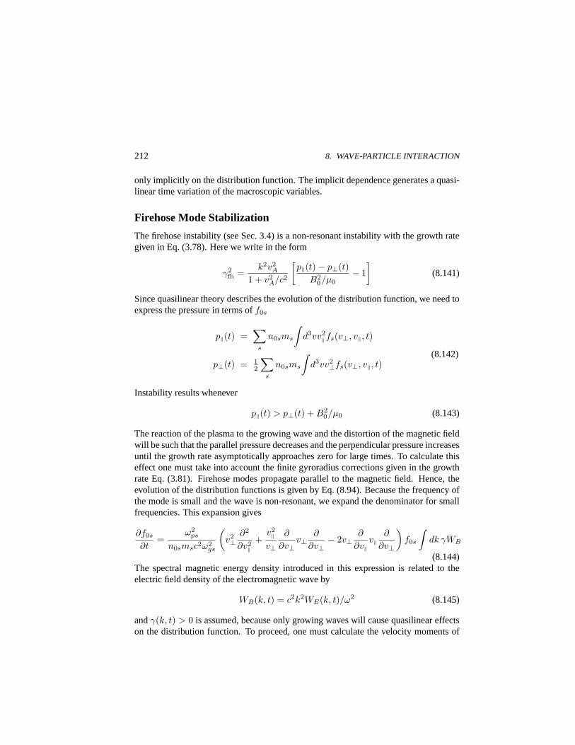
212 8. WAVE-PARTICLE INTERACTION
only implicitly on the distribution function. The implicit dependence generates a quasi-linear time variation of the macroscopic variables.
Firehose Mode Stabilization
The firehose instability (see Sec. 3.4) is a non-resonant instability with the growth rategiven in Eq. (3.78). Here we write in the form
γ2fh =
k2v2A
1 + v2A/c2
[p‖(t)− p⊥(t)
B20/µ0
− 1]
(8.141)
Since quasilinear theory describes the evolution of the distribution function, we need toexpress the pressure in terms off0s
p‖(t) =∑
s
n0sms
∫d3vv2
‖fs(v⊥, v‖, t)
p⊥(t) = 12
∑s
n0sms
∫d3vv2
⊥fs(v⊥, v‖, t)(8.142)
Instability results whenever
p‖(t) > p⊥(t) + B20/µ0 (8.143)
The reaction of the plasma to the growing wave and the distortion of the magnetic fieldwill be such that the parallel pressure decreases and the perpendicular pressure increasesuntil the growth rate asymptotically approaches zero for large times. To calculate thiseffect one must take into account the finite gyroradius corrections given in the growthrate Eq. (3.81). Firehose modes propagate parallel to the magnetic field. Hence, theevolution of the distribution functions is given by Eq. (8.94). Because the frequency ofthe mode is small and the wave is non-resonant, we expand the denominator for smallfrequencies. This expansion gives
∂f0s
∂t=
ω2ps
n0smsc2ω2gs
(v2⊥
∂2
∂v2‖
+v2‖
v⊥
∂
∂v⊥v⊥
∂
∂v⊥− 2v⊥
∂
∂v‖v‖
∂
∂v⊥
)f0s
∫dk γWB
(8.144)The spectral magnetic energy density introduced in this expression is related to theelectric field density of the electromagnetic wave by
WB(k, t) = c2k2WE(k, t)/ω2 (8.145)
andγ(k, t) > 0 is assumed, because only growing waves will cause quasilinear effectson the distribution function. To proceed, one must calculate the velocity moments of

8.6. WEAK MACRO-TURBULENCE 213
the perturbed equation. This yields the quasilinear evolution equations for the hydro-dynamic pressure
dp⊥(t)dt
= p‖(t)∫
dkγ(k, t)WB(k, t)
B20/2µ0
dp‖(t)dt
= −2[2p‖(t)− p⊥(t)]∫
dkγ(k, t)WB(k, t)
B20/2µ0
(8.146)
∂WB(k, t)∂t
= 2γ(k, t)WB(k, t)
Initially, as long as the instability works, one has2p‖ > p⊥, and consequently
dp‖/dt ≤ 0dp⊥/dt ≥ 0
(8.147)
indicating that the parallel pressure decreases from the very beginning while the perpen-dicular pressure increases. The instability cools the plasma in the parallel and heats itin the perpendicular directions as one expects from simple logic. In the long-time limitthe parallel pressure decreases as long until the growth rate vanishes, and one obtainsin the final state some kind of equipartition law for the firehose mode
p‖(∞) = p⊥(∞) + B20/µ0 (8.148)
Because, in addition, the cut-off wavenumber is proportional to the growth rate (seeSec. 3.4),k0(∞) → 0 together with the growth rate. The wavelength of the firehosemode thus increases with time in nonlinear interaction with the plasma.
From Eq. (8.146) we find that the evolution of the two pressure terms follows
dp⊥dp‖
= − p‖/22p‖ − p⊥
(8.149)
If the changes in the pressure close to the stable state att → ∞ are small, this can beexpanded to obtain
p‖(∞)− p‖0 ≈ −Z(0)2p‖0(2p‖0 − p⊥0)p⊥(∞)− p⊥0 ≈ Z(0)p2
‖0(8.150)
whereZ(0) = (p‖0 − p⊥0 −B2
0/µ0)/p‖0(5p‖0 − 2p⊥0) (8.151)
The final spectral energy density in the magnetic field fluctuation follows from theenergy conservation law
12p‖0 + p⊥0 +
∫dkWB(k, t) = const (8.152)
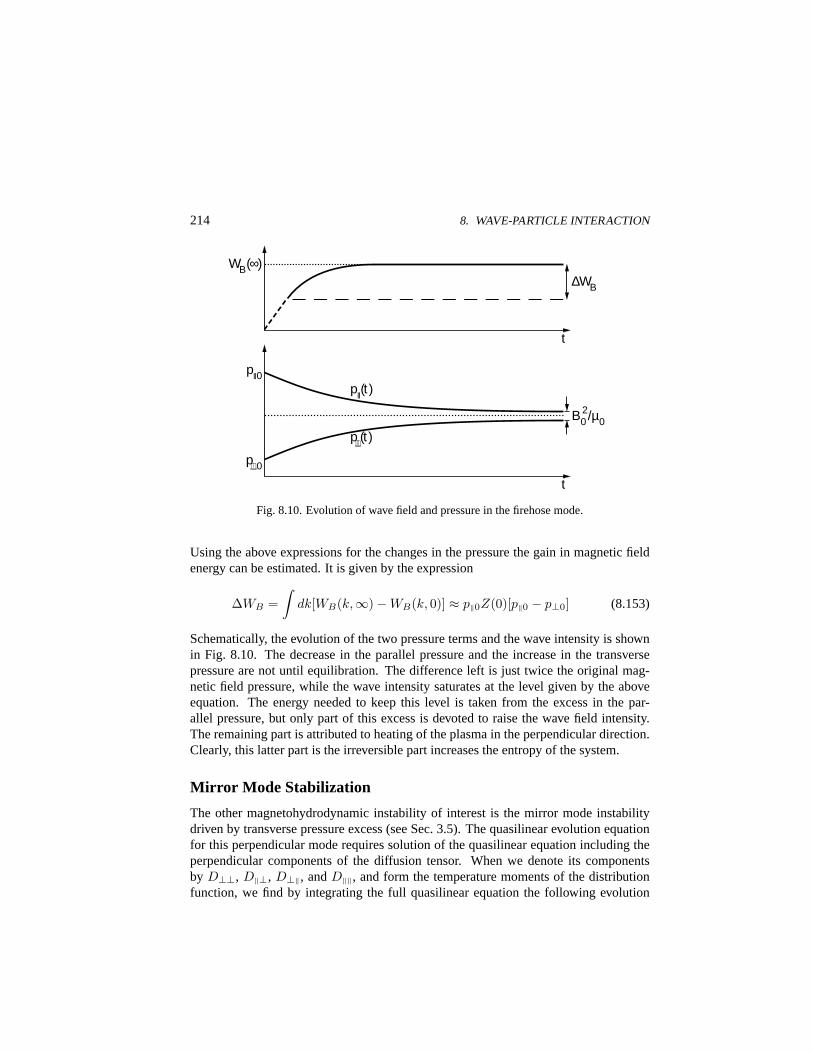
214 8. WAVE-PARTICLE INTERACTION
t
t
B02/µ0
∆WB
WB(∞)
pll(t )
p⊥(t )
pll0
p⊥0
Fig. 8.10. Evolution of wave field and pressure in the firehose mode.
Using the above expressions for the changes in the pressure the gain in magnetic fieldenergy can be estimated. It is given by the expression
∆WB =∫
dk[WB(k,∞)−WB(k, 0)] ≈ p‖0Z(0)[p‖0 − p⊥0] (8.153)
Schematically, the evolution of the two pressure terms and the wave intensity is shownin Fig. 8.10. The decrease in the parallel pressure and the increase in the transversepressure are not until equilibration. The difference left is just twice the original mag-netic field pressure, while the wave intensity saturates at the level given by the aboveequation. The energy needed to keep this level is taken from the excess in the par-allel pressure, but only part of this excess is devoted to raise the wave field intensity.The remaining part is attributed to heating of the plasma in the perpendicular direction.Clearly, this latter part is the irreversible part increases the entropy of the system.
Mirror Mode Stabilization
The other magnetohydrodynamic instability of interest is the mirror mode instabilitydriven by transverse pressure excess (see Sec. 3.5). The quasilinear evolution equationfor this perpendicular mode requires solution of the quasilinear equation including theperpendicular components of the diffusion tensor. When we denote its componentsby D⊥⊥, D‖⊥, D⊥‖, andD‖‖, and form the temperature moments of the distributionfunction, we find by integrating the full quasilinear equation the following evolution
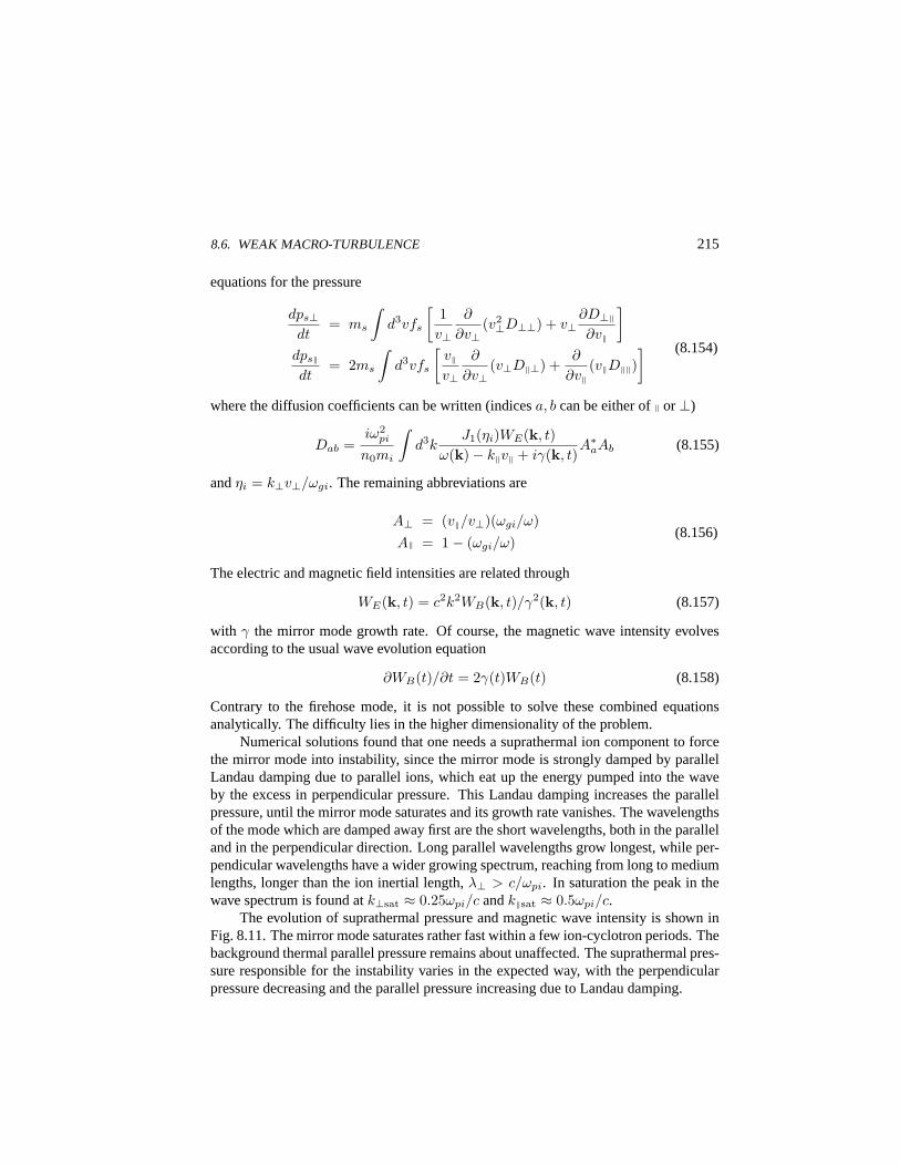
8.6. WEAK MACRO-TURBULENCE 215
equations for the pressure
dps⊥dt
= ms
∫d3vfs
[1v⊥
∂
∂v⊥(v2⊥D⊥⊥) + v⊥
∂D⊥‖∂v‖
]
dps‖
dt= 2ms
∫d3vfs
[v‖v⊥
∂
∂v⊥(v⊥D‖⊥) +
∂
∂v‖(v‖D‖‖)
] (8.154)
where the diffusion coefficients can be written (indicesa, b can be either of‖ or⊥)
Dab =iω2
pi
n0mi
∫d3k
J1(ηi)WE(k, t)ω(k)− k‖v‖ + iγ(k, t)
A∗aAb (8.155)
andηi = k⊥v⊥/ωgi. The remaining abbreviations are
A⊥ = (v‖/v⊥)(ωgi/ω)A‖ = 1− (ωgi/ω)
(8.156)
The electric and magnetic field intensities are related through
WE(k, t) = c2k2WB(k, t)/γ2(k, t) (8.157)
with γ the mirror mode growth rate. Of course, the magnetic wave intensity evolvesaccording to the usual wave evolution equation
∂WB(t)/∂t = 2γ(t)WB(t) (8.158)
Contrary to the firehose mode, it is not possible to solve these combined equationsanalytically. The difficulty lies in the higher dimensionality of the problem.
Numerical solutions found that one needs a suprathermal ion component to forcethe mirror mode into instability, since the mirror mode is strongly damped by parallelLandau damping due to parallel ions, which eat up the energy pumped into the waveby the excess in perpendicular pressure. This Landau damping increases the parallelpressure, until the mirror mode saturates and its growth rate vanishes. The wavelengthsof the mode which are damped away first are the short wavelengths, both in the paralleland in the perpendicular direction. Long parallel wavelengths grow longest, while per-pendicular wavelengths have a wider growing spectrum, reaching from long to mediumlengths, longer than the ion inertial length,λ⊥ > c/ωpi. In saturation the peak in thewave spectrum is found atk⊥sat ≈ 0.25ωpi/c andk‖sat ≈ 0.5ωpi/c.
The evolution of suprathermal pressure and magnetic wave intensity is shown inFig. 8.11. The mirror mode saturates rather fast within a few ion-cyclotron periods. Thebackground thermal parallel pressure remains about unaffected. The suprathermal pres-sure responsible for the instability varies in the expected way, with the perpendicularpressure decreasing and the parallel pressure increasing due to Landau damping.
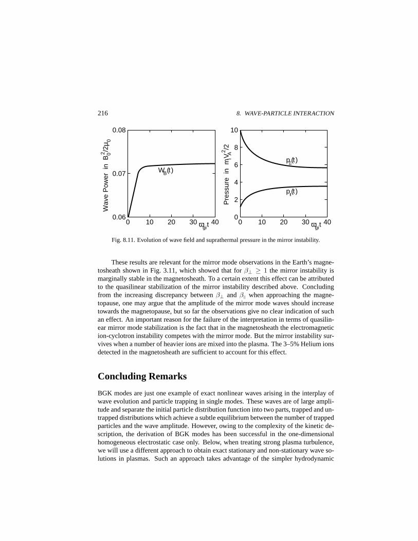
216 8. WAVE-PARTICLE INTERACTION
0.06
0.07
0.08
0 10 20 30 40
Wav
e P
ower
in
B02 /2
µ 0
ωgit
WB(t )
0 0 10 20 30 40
Pre
ssur
e in
miV
A2 /2
ωgit
2
4
6
8
10
pll(t )
p⊥(t )
Fig. 8.11. Evolution of wave field and suprathermal pressure in the mirror instability.
These results are relevant for the mirror mode observations in the Earth’s magne-tosheath shown in Fig. 3.11, which showed that forβ⊥ ≥ 1 the mirror instability ismarginally stable in the magnetosheath. To a certain extent this effect can be attributedto the quasilinear stabilization of the mirror instability described above. Concludingfrom the increasing discrepancy betweenβ⊥ and β‖ when approaching the magne-topause, one may argue that the amplitude of the mirror mode waves should increasetowards the magnetopause, but so far the observations give no clear indication of suchan effect. An important reason for the failure of the interpretation in terms of quasilin-ear mirror mode stabilization is the fact that in the magnetosheath the electromagneticion-cyclotron instability competes with the mirror mode. But the mirror instability sur-vives when a number of heavier ions are mixed into the plasma. The 3–5% Helium ionsdetected in the magnetosheath are sufficient to account for this effect.
Concluding Remarks
BGK modes are just one example of exact nonlinear waves arising in the interplay ofwave evolution and particle trapping in single modes. These waves are of large ampli-tude and separate the initial particle distribution function into two parts, trapped and un-trapped distributions which achieve a subtle equilibrium between the number of trappedparticles and the wave amplitude. However, owing to the complexity of the kinetic de-scription, the derivation of BGK modes has been successful in the one-dimensionalhomogeneous electrostatic case only. Below, when treating strong plasma turbulence,we will use a different approach to obtain exact stationary and non-stationary wave so-lutions in plasmas. Such an approach takes advantage of the simpler hydrodynamic
8.6. WEAK MACRO-TURBULENCE 217
description of the plasma.Trapping of particles in waves may change the wave dynamics in many ways. The
most obvious one is that trapping extracts part of the resonant particles from the dis-tribution function. These particles loose their capability of further feeding instability.Hence trapping will cause stabilization of the instability. But this applies to instabilitiesof single modes. When the bandwidth of the mode becomes large, trapping becomesless important, and other effects set on which we are going to discuss in the next chap-ters. The main remaining effect of trapping is then the distortion of the particle orbitby the broadband spectrum. This causes resonance broadening in wave-particle inter-action.
In this chapter we presented only the wave-particle aspect the weak turbulence the-ory, the zero-order response of the plasma to the presence of a random-phased broad-band spectrum of unstable waves. In addition to quasilinear stabilization of the wavespectrum as result of this response, the deformation of the particle distribution functionimplies a number of effects like particle heating, resonant acceleration, energy diffu-sion, and pitch-angle diffusion, of which only the latter two have been discussed sofar. Clearly, quasilinear weak wave-particle turbulence has a much wider applicationthan mere pitch-angle diffusion. Examples not treated here are the diffusion of cosmicrays across astrophysical plasmas and acceleration of particles in their self-consistentlyexcited low-frequency wave spectra in front of shock waves. In particular, in particleacceleration theory the quasilinear approach has proved to be very useful.
But quasilinear theory has also its drawbacks. For instance, in the context of gen-tle beam stabilization it causes severe problems when applying it to electron streamsejected from the solar corona which are the cause of solar type III radio bursts. Quasi-linear theory would not permit these streams to propagate large distances in the corona,contrary to what is suggested by observation. Thus, quasilinear theory and weak wave-particle turbulence cannot be the last word spoken in nonlinear plasma theory. In thefollowing chapters we explore other nonlinear effects which are ignored in quasilineartheory.
Further Reading
There is a small number of excellent books on nonlinear plasma theory, e.g., [1], [3],[7], and [9], which all were written in the sixties and early seventies. Meanwhile,nonlinear plasma physics has grown into a wide field, but no comprehensive moderntext is available. The reason is that analytical theory has not developed much during thelast twenty years, while the activities and interests have turned to numerical simulations.A contemporary summary of numerical plasma simulations is given in [8].
Particle trapping is described, at least in rudimentary form, in most books on non-linear plasma physics as for instance [1], [7] and [2]. Single wave stabilization for
218 8. WAVE-PARTICLE INTERACTION
Bernstein modes and whistler waves by particle trapping may be found in the originalliterature. The former have been applied in space plasma physics context to radio emis-sion from the Sun during solar type IV bursts. For references consult [4] and [6]. BGKmodes are treated extensively by Davidson [1]. Quasilinear theory is the main sub-ject of most books on nonlinear theory, e.g., [1] and [7]. The ion-cyclotron resonancebroadening saturation theory has been taken from Dum and Dupree,Phys. Fluids13(1970) 2064. Pitch-angle diffusion, as one of the results of quasilinear theory, has wideapplication in space, and even in astrophysics, where it has been applied successfullyto the diffusion theory of cosmic rays. The readers interested more deeply in spaceapplications of pitch angle scattering are referred to [5].
[1] R. C. Davidson,Methods in Nonlinear Plasma Theory(Academic Press, New York,1972).
[2] A. Hasegawa,Plasma Instabilities and Nonlinear Effects(Springer Verlag, Heidel-berg, 1975).
[3] B. B. Kadomtsev,Plasma Turbulence(Academic Press, New York, 1965).
[4] D. J. McLean and N. R. Labrum (eds.),Solar Radiophysics(Cambridge UniversityPress, Cambridge, 1985).
[5] L. R. Lyons and D. J. Williams,Quantitative Aspects of Magnetospheric Physics(D. Reidel Publ. Co., Dordrecht, 1984).
[6] D. B. Melrose,Plasma Astrophysics(Gordon and Breach, New York, 1980).
[7] R. Z. Sagdeev and A. A. Galeev,Nonlinear Plasma Theory(W. A. Benjamin, NewYork, 1969).
[8] T. Tajima,Computational Plasma Physics(Addison-Wesley Publ. Co., RedwoodCity, 1989).
[9] V. N. Tsytovich,Nonlinear Effects in Plasmas(Plenum Press, New York, 1970).

9. Weak Wave Turbulence
Quasilinear theory of wave-particle interaction is only one side of weak turbulencetheory. It is that part dealing with the simplest random-phase reaction of the unstablyexcited wave field on the initial non-equilibrium distribution function. If only this kindof interaction would occur in a plasma, the plasma would approach thermal equilibriumin a straight way. In real plasmas this is by no means the case. In most cases, andlong before quasilinear interaction manages to stabilize the plasma, other modes ofinteraction between the waves themselves come into play. Waves of certain frequenciesand wavenumbers start colliding and exchange momentum and energy. These mutualinteractions among the waves are described by the theory ofwave-wave interaction, theother part of weak turbulence theory.
Wave-wave interaction theory or weak wave turbulence theory, as it is also called,ignores the particle response to the presence and mutual interaction of the waves. Theplasma plays the role of an exciter and wave carrier but is otherwise a passive back-ground, on top of which the various wave processes take place. In this chapter we treatthe waves and their interaction in a manner as if the plasma would be absent, but theproperties of the waves are still determined by the plasma dielectric properties. Wedo not account for wave dissipation in the plasma but for simplicity assume that anydissipation appears only among the waves themselves.
Dissipation is, however, a very important item insofar as it imposes a naturalthreshold on the interaction of the waves and on the nonlinear instabilities which seton when the waves may transform into each other. In most of space plasma physicsthese processes are still out of reach. The presentation given here ignores them becauseof this reason. But under certain conditions, such as heating of plasma in the iono-sphere and the lower corona, and in dissipative wave transformation, neglecting wavedissipation is not justified.
The present chapter presents essentially three different approaches to wave turbu-lence in a plasma: the coherent approach, the incoherent or random-phase approach,and one particular form of incoherent wave interaction theory for the very-low fre-quency range of drift waves, which may be important for the evolution of low-frequencyturbulence in space plasmas.
219
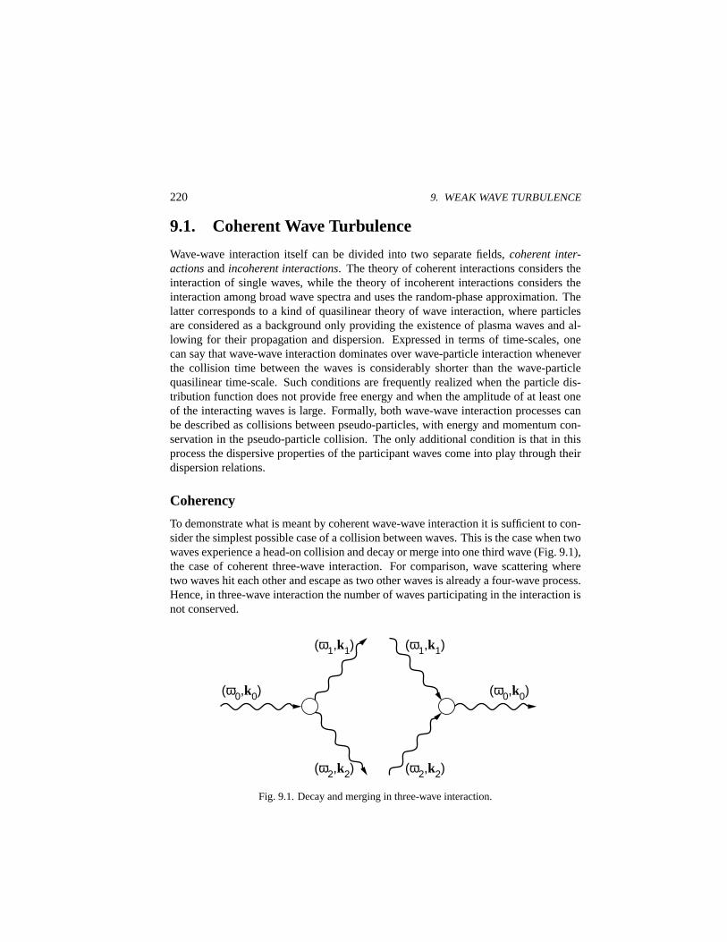
220 9. WEAK WAVE TURBULENCE
9.1. Coherent Wave Turbulence
Wave-wave interaction itself can be divided into two separate fields,coherent inter-actionsandincoherent interactions. The theory of coherent interactions considers theinteraction of single waves, while the theory of incoherent interactions considers theinteraction among broad wave spectra and uses the random-phase approximation. Thelatter corresponds to a kind of quasilinear theory of wave interaction, where particlesare considered as a background only providing the existence of plasma waves and al-lowing for their propagation and dispersion. Expressed in terms of time-scales, onecan say that wave-wave interaction dominates over wave-particle interaction wheneverthe collision time between the waves is considerably shorter than the wave-particlequasilinear time-scale. Such conditions are frequently realized when the particle dis-tribution function does not provide free energy and when the amplitude of at least oneof the interacting waves is large. Formally, both wave-wave interaction processes canbe described as collisions between pseudo-particles, with energy and momentum con-servation in the pseudo-particle collision. The only additional condition is that in thisprocess the dispersive properties of the participant waves come into play through theirdispersion relations.
Coherency
To demonstrate what is meant by coherent wave-wave interaction it is sufficient to con-sider the simplest possible case of a collision between waves. This is the case when twowaves experience a head-on collision and decay or merge into one third wave (Fig. 9.1),the case of coherent three-wave interaction. For comparison, wave scattering wheretwo waves hit each other and escape as two other waves is already a four-wave process.Hence, in three-wave interaction the number of waves participating in the interaction isnot conserved.
(ω0,k0)
(ω1,k1)
(ω2,k2)
(ω0,k0)
(ω1,k1)
(ω2,k2)
Fig. 9.1. Decay and merging in three-wave interaction.

9.1. COHERENT WAVE TURBULENCE 221
Non−deca
y Type
Decay Typ
eFre
quen
cy
Wave Number
Fig. 9.2. Dispersion curves which may and may not yield wave-wave interaction.
Interaction of waves makes only sense if the waves are in resonance. This impliesthe following. Each wave is described by its frequency,ω, and its wavenumber,k. Thefirst corresponds to its energy,hω, the second to its momentum,hk. Conservation oftotal energy and momentum during the collision of the three waves, considered as acollision between three quasi-particles, requires that
ω − ω′ − ω′′ = 0k− k′ − k′′ = 0
(9.1)
Here the three waves are distinguished by the primes. The two conditions (9.1) havethe form of resonant denominators and are therefore called the resonance conditionsor matching conditions, but physically spoken they are the two conservation laws ofenergy and momentum.
Of course, not all waves of arbitrary dispersion can participate in such an inter-action, because satisfying the resonance conditions demands that|k′ + k′′| = |k| ≤|k′| + |k′′|. Hence, three waves belonging to the same dispersion branch can interactonly if this branch is convex from below as shown in Fig. 9.2. Only in this case thetriangle inequality can be satisfied. A high energy mode may decay spontaneously intotwo lower energy modes (left part of Fig. 9.1) of the same kind if the dispersion relationis convex from below, while it cannot decay if it is concave from below.
Decay is, of course, not restricted to the same mode. A given high-energy wavemode with convex dispersion can decay into another wave of its own mode and a low-frequency wave of a different mode. This would be the case for the convex disper-

222 9. WEAK WAVE TURBULENCE
sion relation of Langmuir waves. These waves can easily decay spontaneously into alonger-wavelength, lower-frequency Langmuir wave and, for instance, a much lower-frequency, similar-wavelength ion-acoustic wave. This process is frequently realized innature, whenever the plasma is warm enough to permit the ion-acoustic wave to grow.On the other hand, the inverse process is possible as well, when an ion-acoustic wavecollides with a Langmuir wave to mix the Langmuir frequency up.
Resonant Three-Wave Interaction
The resonant interaction requires that the waves satisfy the linear dispersion relation,ε(k, ωk) = 0; for brevity we indicate the dependence of the frequency on the wavenum-ber by an indexk. We consider the simplest electrostatic and unmagnetized three-waveinteraction case, i.e., Langmuir-ion-acoustic wave interaction. It is clear that the interac-tion causes energy and momentum transfer and thus produces small shifts in frequency,∆ω, and wavenumber,∆k, from the initial (linear) values,k0, ωk0 . Expansion of thedispersion relation around the initial values gives for the variation ofε
δε(k) = Re δε(k0) + iIm δε(k0) +∂δε
∂ω
∣∣∣∣k0
∆ω +∂δε
∂k
∣∣∣∣k0
·∆k (9.2)
For electrostatic waves it is most convenient to consider the variation of the electrostaticpotential. The latter becomes a function of time,τ , related to the frequency shift, andspace,ξ, related to the wavenumber shift. With this in mind we can replace the shiftsby the equivalent operators∆ω → i∂/∂τ and∆k → −i∇ξ, where∇ξ = ∂/∂ξ isthe spatial gradient operator acting on the displacement vector,ξ. Moreover, using thegroup velocity
vgr0 = ∂ωk/∂k|k=k0(9.3)
and interpreting the variation of the dielectric function as an operator acting on thevariation of the potential, one obtains the following equation for the potential amplitude
δε(k)δφ(k0) = i∂ε
∂ω0
(∂
∂τ ′− γ0
)δφ(k0) (9.4)
where the following abbreviations have been used
∂
∂τ ′=
∂
∂τ− vgr0 · ∇ξ
∂ε
∂ω0=
∂[Re δε(k)]∂ωk
∣∣∣∣k=k0
(9.5)
γ0 = − Im δε(k)(∂ε/∂ω0)
9.1. COHERENT WAVE TURBULENCE 223
The quantityγ0 is clearly the linear growth rate of the wave with frequencyω(k0).This interpretation is easy to understand. The dispersion relation of electrostatic wavesresults from the equationεδφ = 0 for non-vanishing potential amplitude. Thus, whenthe linear dispersion relation is satisfied for the initial wave, the remaining relation isthe product of the two distortions. This nonlinear term has been neglected in the devel-opment of the linear theory. The wave-wave interaction theory is thus, from the pointof view of an expansion with respect to amplitudes, the first step of a true nonlineartheory. Since the distortion of the dielectric function depends on space and time, it be-comes an operator acting on the distortion of the wave field. This is the content of theabove nonlinear differential equation forδφ.
Coupled Wave Equations
We have found a representation of the nonlinear operator with the unprimed wave asthe modified wave. The wave system consists of three waves, however. Hence, the fulldispersion relation depends on all tree waves, implying that we must vary it with respectto the three wave amplitudes. This yields up to the second-order variation
δε(k)δφ(k) +∑
k=k′+k′′δε(k′,k′′)δφ(k′)δφ(k′′) = 0 (9.6)
where we made use of the condition that in the coupling term only such couplingsappear which satisfy the conservation laws. Moreover, taking only a sum over threewaves in the second term restricts the consideration to three-wave interactions. Higherorder interactions would provide addition sums. If we now substitute Eq. (9.5) into Eq.(9.6), we obtain the following coupled equations
(∂
∂τ ′− γ0
)∂ε
∂ω0δφ(k0) = iδε(k0,k1,k2)δφ(k1)δφ(k2)
(∂
∂τ ′− γ1
)∂ε
∂ω1δφ(k1) = iδε(k1,−k2,k0)δφ(−k2)δφ(k0) (9.7)
(∂
∂τ ′− γ2
)∂ε
∂ω2δφ(k2) = iδε(k2,k0,−k1)δφ(k0)δφ(−k1)
This system results by taking each of the three waves as the initial one and letting itcollide with the two others. Moreover, since the wave fields are real,δφ(−k) = δφ(k)∗.Because each of the three waves can play the role of the initial wave, it is convenientto symmetrize these three evolution equations for the three wave amplitudes under theaction of the two other waves. We define a normalized complex wave amplitude
A(kj ; τ, ξ) = δφ(kj ; τ, ξ)
∣∣∣∣∣∂(ωε)∂ω(kj)
ε0k2j
2ω(kj)
∣∣∣∣∣
1/2
(9.8)

224 9. WEAK WAVE TURBULENCE
The derivative ofε in this expression is the expression which enters the fluctuationenergy in one wave mode given in Eq. (2.19). The sign of the wave amplitude canbe positive or negative and is determined as the sign of the derivative of the dielectricfunction
sgn(∂ε/∂ωj) = S(kj) (9.9)
such that the spectral energy density isW (kj), and the wave action can be written as
S(kj)|A(kj)|2 = W (kj)/ω(kj) = hN(kj) (9.10)
whereN(kj) is the number of wave quanta contained in the mode of wavenumberkj .Since the time derivative of the action is the energy, the new abbreviations can be usedto write the above system of equations in its simplest symmetrized form
S(k0)∂A(k0)/∂τ ′ = −iV A(k1)A(k2)S(k1)∂A(k1)/∂τ ′ = −iV A(k0)A(k∗2) (9.11)
S(k2)∂A(k2)/∂τ ′ = −iV A(k∗1)A(k0)
The common factor,V = V (k0,k1,k2), on the right-hand sides of these equationsis the three-wave coupling coefficient. The three wave modes have been numberedconsecutively here. The coupling coefficient written satisfies the following symmetries
V (k1,−k2,k0) = V (k2,k0,−k1) = V (k0,k1,k2) (9.12)
and is given by the rather complicated expression
V (k0,k1,k2) =√
2k20ε(k0,k1,k2)
ε0 |[k20∂ε/∂ω(k0)][k2
1∂ε/∂ω(k1)][k22∂ε/∂ω(k2)]|1/2
(9.13)
Wave Decay
These expressions close the system of equations for the amplitudes of the three waves.All three waves are coupled, but because we have neglected all other ingredients in theinteraction apart from just these three waves, the total energy in this interaction andthe total momentum is necessarily conserved. This conservation can be checked byexpressing the complex amplitude by its modulus and a phase as
A = |A(τ)| exp[iθ(τ)] (9.14)
Introducing this ansatz into the above system of equations, it can be reduced to the fol-lowing form (for simplicity we use the subscripts 0, 1, 2, instead of the wavenumbers)
S0∂|A0|/∂τ = −V |A1||A2| sin θ
S1∂|A1|/∂τ = +V |A0||A2| sin θ (9.15)
S2∂|A2|/∂τ = +V |A0||A1| sin θ
9.1. COHERENT WAVE TURBULENCE 225
and another equation for the time variation of the phase
∂θ/∂τ = V cos(θ0 − θ1 − θ2)∂[ln(|A0||A1||A2|)]/∂τ (9.16)
These equations determine the constants of motion during the interaction of the threewaves. The last equation immediately gives
|A0||A1||A2| cos θ = const (9.17)
The amplitude equations can, after multiplication with the appropriate amplitudes ofthe waves and addition as well as using the resonance conditions, be managed to bebrought into the form of an energy density conservation law
W0 + W1 + W2 = const (9.18)
Also, integration of the amplitude equations (9.15) yields the conservation equations ofthe wave occupation numbers
N0 + N1 = constN0 + N2 = const (9.19)
N1 −N2 = const
These latter equations are equivalent to the creation and annihilation processes of oc-cupations of states known from quantum field theory. Actually, taking one quantumaway from the 0-mode, it appears in the 1- and 2-modes such that∆N0 = −1 causes∆N1 = ∆N2 = 1, a process which describes the decay of the 0-mode. Such decayprocesses may stabilize an instability of the 0-mode. To demonstrate how this happens,let us assume that|A0| is much larger initially than the amplitudes of the other twowaves. In this case we can linearize the amplitude equations (9.15) in a decay process,in which the 0-mode can be considered to be a quasi-constant pump wave, the 1- and2-modes both turn out to grow linearly in time according to
|A1,2| ∝ exp[V |A0|τ ] (9.20)
Of course, this linear growth phase is valid only for the short initial time interval, aslong as the 0-mode does not loose too much energy. The more exact solution to theabove system of equation with initial condition|A0(0)|2 = N0(0) À N1(0) and|A2(0)|2 = N2(0) = 0 can be expressed in terms of elliptic functions. Clearly, theprocess involving only three waves is a purely reversible process. The two small am-plitudes grow in time on the expense of the pump wave. When the energy of the pumpwave is consumed, the daughter waves start pumping energy back into the mother wave,and so on, as long as no dissipation is involved. Figure 9.3 shows the strictly reversibleevolution of the occupation numbers of the three waves.
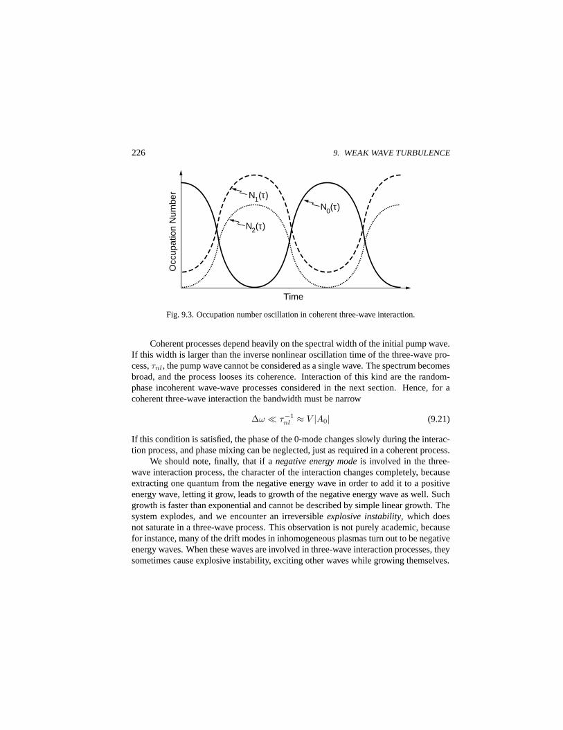
226 9. WEAK WAVE TURBULENCE
Time
Occ
upat
ion
Num
ber N1(τ)
N2(τ)
N0(τ)
Fig. 9.3. Occupation number oscillation in coherent three-wave interaction.
Coherent processes depend heavily on the spectral width of the initial pump wave.If this width is larger than the inverse nonlinear oscillation time of the three-wave pro-cess,τnl, the pump wave cannot be considered as a single wave. The spectrum becomesbroad, and the process looses its coherence. Interaction of this kind are the random-phase incoherent wave-wave processes considered in the next section. Hence, for acoherent three-wave interaction the bandwidth must be narrow
∆ω ¿ τ−1nl ≈ V |A0| (9.21)
If this condition is satisfied, the phase of the 0-mode changes slowly during the interac-tion process, and phase mixing can be neglected, just as required in a coherent process.
We should note, finally, that if anegative energy modeis involved in the three-wave interaction process, the character of the interaction changes completely, becauseextracting one quantum from the negative energy wave in order to add it to a positiveenergy wave, letting it grow, leads to growth of the negative energy wave as well. Suchgrowth is faster than exponential and cannot be described by simple linear growth. Thesystem explodes, and we encounter an irreversibleexplosive instability, which doesnot saturate in a three-wave process. This observation is not purely academic, becausefor instance, many of the drift modes in inhomogeneous plasmas turn out to be negativeenergy waves. When these waves are involved in three-wave interaction processes, theysometimes cause explosive instability, exciting other waves while growing themselves.
9.2. INCOHERENT WAVE TURBULENCE 227
9.2. Incoherent Wave Turbulence
The previous section dealt with the coherent case, considering single waves. The sit-uation becomes fundamentally different when many waves of different phases are in-volved in the interaction process. In such a case the conservation laws are not satisfiedindependently in each particular case of interaction, but in the average over all phasesin the global interaction. This does not mean that they are not satisfied microscopically,it means only that there is no information available over the exact microscopic inter-action to the outer world. The information is provided in such a way that the energyand momentum conservation laws are satisfied globally, while it is not important toknow which waves exactly had interchanged their momenta and energies at a particularinstant of time.
Random-Phase Wave-Wave Interaction
When Eq. (9.21) is strongly violated, the wave spectrum is broad enough to providesufficient phase mixing, and the interaction between the waves can be described in astatistical version of weak turbulence theory, where the phases are considered to berandomly distributed in exactly the same manner as in weakly turbulent wave-particleinteraction theory. In such a case the wave amplitude is represented as superposition ofmany waves, and the time averaged amplitude,〈A(k)〉 = 0, vanishes because the phaseof the wave varies much faster than the amplitude factor
〈A(k, τ)〉 = limT→∞
1T
∫ T
0
A(k, τ) exp[iθ(t)]dt = 0 (9.22)
This integral is zero because the slowly variable amplitude factor with time scaleτcan be extracted from the integral. The presence of many waves with different wavenumbers in the random-phase approximation then implies that in the equations for thewave amplitudes (9.11) we sum over all possible combinations of wavenumbers satis-fying the momentum conservation condition. But in addition we must permit for smallfrequency shifts,∆ω(k), which may arise in the interaction. These shifts correspondto energy uncertainties caused by the random phases. The interacting waves do notknow precisely with which phase they have interacted. Of course, these mismatches infrequency are not free, but must satisfy the conservation laws as well.
The general theory for many-wave interaction is very complicated. We thus willdiscuss only the random-phase or incoherent weakly turbulent three-wave interactionprocess. Summing over all possible combinations of wavenumbers gives
S0∂A0
∂t= −i
∑
k0=∆0
V (k0,k′,k′′)A(k′)A(k′′) exp(i∆ω0t)
228 9. WEAK WAVE TURBULENCE
S1∂A1
∂t= −i
∑
k1=∆1
V (k1,−k′′,k)A(−k′′)A(k) exp(−i∆ω1t) (9.23)
S2∂A2
∂t= −i
∑
k2=∆2
V (k2,k,−k′)A(k)A(−k′) exp(−i∆ω2t)
The definitions of the quantities are the same as in the foregoing section, and the mis-matches and summation conditions are
∆0 = k′ + k′′
∆1 = k− k′′ (9.24)
∆2 = k− k′
and
∆ω0 = ω(k0)− ω(k′)− ω(k′′)∆ω1 = ω(k)− ω(k1)− ω(k′′) (9.25)
∆ω2 = ω(k)− ω(k2)− ω(k′)
For a continuous broad spectrum one can replace the sums in these expressions byintegrals over the primed wavenumbers and introduce aδ-function taking care of theresonances. Then the master equation for an amplitude is of the form
S0∂A0
∂t=
∫ ∫d3k1d
3k2δ(k0 − k1 − k2)V A1A2 exp[i∆ω0t] (9.26)
whereV = V (k0,k1,k2) is the three-wave coupling coefficient defined in Eq. (9.13).The equations for the two other wave amplitudes are obtained by permutation of theindices and observation of the symmetries inV .
Amplitude Equations
In the framework of a perturbation approach we assume that in any of the integrationsor summations performed, the amplitudes under the integrals or sums can be consid-ered to be slowly variable and can therefore be held constant in the time integration.Calculating the square of the amplitude by multiplication with the complex conjugate,one obtains for the energy density or occupation number of the 0-mode
∂|A0|2∂t
= −iS0
∑
k0=k1+k2
[V 〈A∗0A1A2 exp(i∆ω0t)〉 − V ∗ 〈A0A∗1A
∗2 exp(−i∆ω0t)〉]
(9.27)

9.2. INCOHERENT WAVE TURBULENCE 229
and similar expressions for the energy densities of the other modes. In this formula thereappear time averages over three amplitudes. The amplitudes to be used are calculatedfrom the amplitude equations (9.23) in the manner indicated above by assuming thatthe product of amplitudes appearing in their integrands varies slowly and can be con-sidered to be constant. The remaining integrals contain exponentials of the frequencymismatches and thus produce resonant denominators∆ω0,1,2 +iδ, where a small imag-inary part is added to make the integrals converge. This imaginary part will later be setto zero. In the random-phase approximation one now assumes that any average of aproduct of amplitudes satisfies a condition like
〈A1A2〉 = |A1|2δ(k1 + k2) (9.28)
where, since the wave amplitudes are real quantities, we also haveA(−k) = A∗(k).All the coupling coefficients,V , become symmetric functions of the wavenumbers un-der this condition. Moreover, we replace the resonant denominators using Plemelj’sformula (see Eq. (I.A.78) in the appendix of our companion book) by
(∆ω ± iδ)−1 = P/∆ω ∓ iπδ(∆ω) (9.29)
with P indicating the principal value, and theδ-function taking care of the exact res-onance and energy conservation (note that theδ-function arises exclusively from thesmall imaginary part,iδ, in the resonant denominator in the limitδ → 0). Carrying outall these calculations, Eq. (9.27) becomes
∂|A0|2∂t
= 4πS0
∑
∆k0
|δ(∆ω0)V |2[S0|A1|2|A2|2 − S1|A0|2|A2|2 − S2|A0|2|A1|2
]
(9.30)and similar equations for the energy densities of the remaining wave modes. For abroad spectrum it is convenient to replace the sum by an integral. In order to do this onedefines, as in Eq. (9.26), continuous spectral energy densities,|Aj |2 → hN(k)jd
3kj ,which are expressed in the number densities of the photons contained in the particularmodej = 0, 1, 2, as given in Eq. (9.10). Moreover, when transforming the sum into anintegral one must take care of the restriction of the summation due to the requirementof the conservation of the wave momentum, which is expressed in the fact that thesums are taken only over the values∆k0, etc. Hence, in the integral appears anotherδ-function, i.e.,δ(k0 − k1 − k2) = δ(∆k0) and similar expressions for the other twomodes
∆k0 = k0 − k1 − k2
∆k1 = k1 − k2 − k0 (9.31)
∆k2 = k2 − k0 − k1
230 9. WEAK WAVE TURBULENCE
After all these preliminaries, we are now in the position to perform this transformation.As result the equation for the number density of wave quanta in the 0-mode is obtained
∂N0
∂t= 4πS0
∫ ∫d3k1d
3k2 |V |2 [S0N1N2 − S1N0N2 − S2N0N1] δ(∆k0)δ(∆ω0)
(9.32)The corresponding equations for the other quantum occupation numbers are obtainedby permutations (forN1 : 0→1, 1→−2, 2→0, for N2 : 0→2, 1→0, 2→−1) and ob-serving the symmetry relations,S−0 = −S0, V (0, 1, 2) = V (1,−2, 0) = V (2, 0,−1),andN(−k) = N(k), with S−0 = S(−k0), from Eq. (9.10)
∂N1
∂t= −4πS1
∫ ∫d3k0d
3k2|V |2 [S0N1N2 − S1N0N2 − S2N0N1] δ(∆k0)δ(∆ω0)
∂N2
∂t= −4πS2
∫ ∫d3k0d
3k1|V |2 [S0N1N2 − S1N0N2 − S2N0N1] δ(∆k0)δ(∆ω0)
(9.33)
The integrands of these three last equations (9.32) and (9.33) are identical. Only signsand integration variables have changed. Taken together these are thewave kinetic equa-tionsfor incoherent three-wave interaction.
The wave kinetic equations resemble the coherent wave equations (9.11). Thereare two important differences between the coherent and the incoherent descriptions.The first concerns the coupling time scale of evolution of the wave energies or ampli-tudes. In the coherent case the time scale is inversely proportional to the amplitude ofthe wave while in the incoherent random-phase case it is inversely proportional to theenergy of the wave or, equivalently, the number density of wave quanta. This impliesthat the coherent time scale of the evolution is much shorter than the incoherent timescale. Coherent systems evolve much faster than incoherent systems. In addition, thecoherent evolution was strictly reversible, while the incoherent interaction of the wavesis irreversible. In the random-phase interaction the waves forget what their initial phasehas been, and the systems can never return to this initial state. This can be demonstratedby defining an entropy function for the random-phase interaction as
S(t) =∑
j=0,1,2
∫d3k ln Nj(kj) (9.34)
Differentiating with respect to time and inserting the wave kinetic equations into thisform yields an ever-positive right-hand side such thatdS/dt ≥ 0, which implies that theentropy will always grow, and the system is irreversible. The condition for a stationaryfinal state is found to be given by
S0
N0− S1
N1− S2
N2= 0 (9.35)

9.3. WEAK DRIFT WAVE TURBULENCE 231
which must be satisfied for each particular set of wavenumbers and frequencies satisfy-ing the energy and momentum conservation laws or the resonance conditions. This sta-tionary state implies some kind of equipartition between the quanta in the wave modes.
9.3. Weak Drift Wave Turbulence
The general theory of wave turbulence developed in the previous sections can be appliedto all cases of wave interaction. Here we consider the particular case of drift waves inthe plane perpendicular to the magnetic field, where a special two-dimensional kineticwave equation can be derived. It describes drift wave turbulence and is important inspace plasma applications where long wavelength modes are relevant in the particleand energy diffusion processes.
Drift Wave Equations
The drift wave equation applies to the very low frequency range below the ion-cyclotronfrequency,ω < ωgi, which is of interest for large-scale plasma turbulence. The long-wavelength range is defined as the domain of wavenumberskcia/ωgi ¿ 1. The wavespectrum at shorter wavelengths, wherekcia/ωgi ≈ 1, is caused by scattering of thelong-wavelength mode. For the shorter wavelength part of the spectrum it is necessaryto include the inhomogeneity of the plasma. What we are interested in is the evolutionequation for this spectrum.
Turning to a fluid description, the following model equations are used as startingpoint. Electrons are considered in the magnetized drift approximation with negligibleinertia parallel to the magnetic field
∂δn
∂t+∇⊥ · (n0vd) = 0 (9.36)
wheren0 is the unperturbed density,vd = vE + vP is the sum of the electric fieldand polarization drifts defined in Eqs. (1.10) and (1.11), and∇⊥ is the perpendiculargradient operator. The electric field and thus the polarization drift is expressed throughthe electric potential,φ, but includes the full nonlinearity caused by the transverse con-vective derivative
vE = −∇⊥φ×B0
B20
vP = − 1ωgiB0
[∂
∂t∇⊥ + (vE · ∇⊥)∇⊥
]φ
(9.37)
232 9. WEAK WAVE TURBULENCE
Parallel to the magnetic field the electrons obey Boltzmann’s equation
δn
n0=
eφ
kBTe(9.38)
The nonlinearity in the polarization drift of the ions is the driving force for the nonlinearcoupling.
Hasegawa-Mima Equation
From this set of equations one can derive a nonlinear equation. Using the identity
∇ · [(e‖ ×∇φ) · ∇]∇φ = [(e‖ ×∇φ) · ∇]∇2φ (9.39)
and normalizingn, t,x, φ to n0, 1/ωgi, cia/ωgi, kBTe/e, respectively, the above sys-tem of equations can be reduced to the following nonlinear equation forφ
∂
∂t(∇2φ− φ) = −[(e‖ ×∇φ) · ∇]∇2φ (9.40)
This is theHasegawa-Mima equation. It describes the temporal and spatial evolutionof the potential of nonlinear drift waves in the very low-frequency approximation. TheHasegawa-Mima equation is very similar to an equation describing incompressible hy-drodynamic turbulence, but Eq. (9.40) describes turbulence of drift waves in compress-ible plasma physics, with the compression given by the field-aligned electron motion.
Constants of Motion
The Hasegawa-Mima equation (9.40) has two constants of motion which indicate thatthere are two different inertial ranges. These constants of motion are obtained by multi-plying Eq. (9.40) byφ and integration over the entire volume. Then the nonlinear termbecomes
∫d3xφ[(e‖ ×∇φ) · ∇]∇2φ =
∫d3x∇ · [φ∇2φ(e‖ ×∇φ)] (9.41)
This expression can be transformed into a surface integral. Thus one finds that
∂W1
∂t=
12
∂
∂t
∫d3x [φ2 + (∇φ)2] = −
∫j1 · dA (9.42)
where the current density is given by
j1 = −φ∇∂φ
∂t+
12(∇2φ)2e‖ ×∇φ (9.43)
9.3. WEAK DRIFT WAVE TURBULENCE 233
In non-normalized variablesn = n0eφ/kBTe andv2E = (∇φ)2/B2
0 , we find for thefirst conserved quantity, which turns out to be the total energy
W1 = (n2kBTe/n0 + min0v2E)/2 (9.44)
The second conserved quantity is obtained by multiplying Eq. (9.40) by∇2φ
∂W2
∂t=
12
∂
∂t
∫d3x [(∇φ)2 + (∇2φ)2] = −
∫j2 · dA (9.45)
where the second current density is given by
j2 = ∇φ∂φ
∂t+
12(∇2φ)2e‖ ×∇φ (9.46)
It can also be shown that the second conserved quantity,W2 = Wkin + Ω2, is the sumof the kinetic energy and the squaredvorticity
Ω2 = (∇× vE)2 = (∇2φ)2(kBTe/eB0)2 (9.47)
Adding up both constants,W3 = W1 + W2, gives as an alternative conserved quantitythe expression
W3 =[
n
n0− (∇× vE)2
e2B20
k2BT 2
e
]2
(9.48)
This is the squaredenstrophyin a compressible two-dimensional medium as can beseen from the following derivation. Write the ion equation of motion
midvi
dt= e(E + vi ×B)− 1
n∇p (9.49)
and consider an electromagnetic perturbation. Let us define the vorticity vector asΩ = ∇ × vi + (e/mi)B. Taking the curl of the above equation, using Faraday’slaw, ∂E/∂t = −∇×B, and the identityv · ∇v = 1
2∇v2 − v ×∇× v, one gets
∂Ω∂t
−∇× vi ×Ω =1
min2∇n×∇p (9.50)
The divergence of the vorticity vanishes,∇ ·Ω = 0. Therefore we have for the curl ofthe cross product of velocity and vorticity,∇×v×Ω = −Ω∇·v+Ω ·∇v−v ·∇Ω.The second term in this expression vanishes because there is no variation of the velocityin the direction of the vorticity, and the above equation for the vorticity transforms into
dΩdt
+ Ω∇ · vi =1
min2∇n×∇p (9.51)
234 9. WEAK WAVE TURBULENCE
For a cold ion fluid the ion pressure vanishes. Using the continuity equation to expressthe divergence of the ion velocity∇× vi = −d(ln n)/dt, one finds
d
dt
(Ωn
)2
= 0 (9.52)
an equation which expresses conservation of enstrophy in a compressible fluid. Nowusing Boltzmann’s distribution for the densityn this expression reduces to the conser-vation of the quantityW3, showing that the compressible enstrophy is conserved by theHasegawa-Mima equation.
Kinetic Drift Wave Equation
The first step in the derivation of the nonlinear kinetic wave equation is standard andfollows the procedure discussed in the previous sections. One expands the electric wavepotential function into a spatial Fourier series
φ(x, t) = 12
∑
k⊥
[φ(k⊥, t) exp(ik⊥ · x) + c.c.] (9.53)
Let us normalize time to the inverse ion gyroperiod,1/ωgi, and lengths tocia/ωgi. Thisimplies that the frequencies are normalized to the ion-cyclotron frequency,ω/ωgi → ω.The Fourier ansatz transforms the above set of nonlinear equations into the followingevolution equation for the spatial Fourier amplitudes
∂φ(k, t)∂t
+ iωd(k)φ(k, t) = 12
∑
∆k=0
V (k,k′,k′′)φ(k′, t)φ(k′′, t) (9.54)
where∆k = k− k′ − k′′ and where we explicitly indicated thek- andt-dependences,but dropped the⊥-sign onk. The interaction matrix is given by
V (k,k′,k′′) =k′′2 − k′2
1 + k2e‖ · (k′ × k′′) (9.55)
The new frequency,ωd, is the drift wave frequency normalized to the ion-cyclotronfrequency,ωgi, and given by
ωd(k) = − kBTe
ωgieB0
k⊥Ln
1 + k2(9.56)
with Ln = 1/∇⊥(lnn0) the gradient scale length.Because of the assumption of very small parallel wavenumbers,k‖ ≈ 0, Eq. (9.54)
describes two-dimensional electrostatic low-frequency drift wave turbulence in magne-tized plasmas. The drift frequency appearing in this equation plays somewhat the role
9.3. WEAK DRIFT WAVE TURBULENCE 235
of a viscosity. For very smallk the right-hand side can be dropped and the problembecomes a linear one, with the dominating linear term yieldingω = ωd and no wave-wave interaction present. For very large normalizedk À 1 the drift wave frequencyvanishes, and the linear term must be replaced by some kind of viscosity or ion Landaudamping. Here the wave energy is dissipated. This is logical because one expects thatdamping occurs at very short wavelengths. The turbulent state belongs to wavenumbersclose tok ≈ 1, when all the couplings are included.
One can solve the above equation using the methods of weak turbulence by as-suming that a large-amplitude wave exists initially at very long wavelengths. The firststep is to integrate Eq. (9.54) with respect to time to obtain
φ(k, t) = 12
∑
∆k=0
V (k,k′,k′′)
t∫
0
dt′ φ(k′, t)φ(k′′, t) exp[−iωd(k)(t− t′)] (9.57)
In order to find an equation for the root-mean square amplitude, we follow the usualprocedure by multiplying Eq. (9.54) by the conjugate complex functions,φ∗(k, t), andadding the complex conjugate product. Then one obtains the symmetric equation
∂
∂t|φ(k, t)|2 =
12
∑
∆k=0
V (k,k′,k′′)[φ(k′, t)φ(k′′, t)φ∗(k, t) + c.c.] (9.58)
This last equation determines the evolution of the wave intensity. One now substitutesthe integrated version of the wave potential in Eq. (9.57) for each of the amplitudes,φ, into Eq. (9.58). Subsequently one takes the ensemble average of the resulting ex-pression. Because we assume a broad spectrum, we can apply the random-phase ap-proximation of the incoherent wave-wave interaction. This approximation produces atwo-point correlation function on the right-hand side which can be written as
〈φ(k, t)φ(k′, t)〉 = δ(k− k′)|φ(k, t)|2 exp[−(iω + γ)(t− t′)] (9.59)
The damping rate,γ, of the two-point correlation function has been introduced explic-itly. As we know from incoherent interaction theory, it is necessary to introduce this asa decoherence parameter in order to obtain non-diverging results. If we now follow theindicated path, substituting Eq. (9.57) into Eq. (9.58), and using Eq. (9.59), we obtainthe wave kinetic equation of weak low-frequency drift wave turbulence
∂
∂t|φ(k, t)|2 =
12
∑
k′V (k,k′,k− k′)
[V (k,k′,k− k′)
γ(k′) + γ(k− k′)|φ(k′)|2|φ(k− k′)|2
V (k,k,−k′)γ(k) + γ(k′)
|φ(k)|2|φ(k′)|2 +V (k,k,k′ − k)
γ(k) + γ(k′ − k)|φ(k)|2|φ(k′ − k)|2
](9.60)

236 9. WEAK WAVE TURBULENCE
This is thedrift wave kinetic equationfor the wave-coupling in two-dimensional driftwave turbulence in a magnetized plasma, with the turbulence being in the plane perpen-dicular to the magnetic field. It is thek-space version of the Hasegawa-Mima equation(9.40). Interpreting the three terms on the right-hand side shows that the first termis the mode coupling term, while the two other terms describe the self-interaction ofthe wave, which without the introduction of the imaginary damping part would lead todivergence.
Spectral Evolution
Let us assume that a large-amplitude drift wave of initial potential amplitudeφ(k0) and|φ(k0)|2 À |φ(k)|2 has been excited by some instability mechanism. One particularexample of such drift waves would be lower-hybrid drift modes. This wave is of longwavelength,|k0| ¿ 1, corresponding to injection of wave energy at small wavenum-bers. Moreover, we assume that the damping of the initial wave is much smaller thanthe damping of the shorter wavelengths waves,|γ(k0)| ¿ |γ(k)|. Under these condi-tions one can linearize the above wave kinetic equation (9.60) with respect to the weakshort-wave intensity in order to determine the spectral width of the shorter waves. Tothis end we need the intensity of the shorter waves. This is obtained exactly along thesame lines as in the previous section. We multiply Eq. (9.54) by its conjugate com-plex and use Eq. (9.57) to obtain an equation for the correlation of the small amplitudeshort-wave spectrum
[∂
∂t+ iωd(k)− |φ(k0)|2
4γ(k)V (k,k0,k− k0)V (k,k,−k0)
]〈φ(k, t)φ∗(k, t)〉 = 0
(9.61)Using Eq. (9.59) yields the following equality
2γ2(k) =12
(k× k0)2
1 + k2
(k2 − 2k · k0)(k2 − k20)
1− (k− k0)2|φ(k0)|2 (9.62)
from where one obtains for the damping rate
γ(k) =1
23/2
k0k3
1 + k2
[1− k2
0
k2
(k2 − k21)(k
2 − k22)
1 + k2
]|φ(k0)| (9.63)
wherek21,2 = −1 ± 1/
√2 and we have assumed that|φ(k)|2 is isotropic, such that it
is allowed to average over the angle betweenk andk0. Only the lowest-order term ink20/k2 is retained. As one observes, for small wavenumbers the spectral width behaves
like γ ∝ k3. On the other handω ∝ k. Hence, the width may become smaller than thefrequency, in contradiction to our assumption of small frequency. This sets a limitationon the theory.
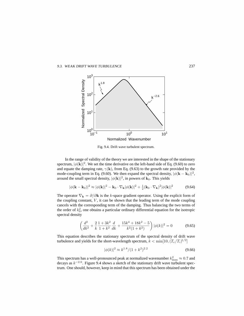
9.3. WEAK DRIFT WAVE TURBULENCE 237
100
10−1 100 101
101
102
103
k1.8
k−2.6
Normalized Wavenumber
Nor
mal
ized
Spe
ctra
l Den
sity
Fig. 9.4. Drift wave turbulent spectrum.
In the range of validity of the theory we are interested in the shape of the stationaryspectrum,|φ(k)|2. We set the time derivative on the left-hand side of Eq. (9.60) to zeroand equate the damping rate,γ(k), from Eq. (9.63) to the growth rate provided by themode-coupling term in Eq. (9.60). We then expand the spectral density,|φ(k − k0)|2,around the small spectral density,|φ(k)|2, in powers ofk0. This yields
|φ(k− k0)|2 ≈ |φ(k)|2 − k0 · ∇k|φ(k)|2 + 12 (k0 · ∇k)2|φ(k)|2 (9.64)
The operator∇k = ∂/∂k is thek-space gradient operator. Using the explicit form ofthe coupling constant,V , it can be shown that the leading term of the mode couplingcancels with the corresponding term of the damping. Thus balancing the two terms ofthe order ofk2
0, one obtains a particular ordinary differential equation for the isotropicspectral density
(d2
dk2+
2k
1 + 3k2
1 + k2
d
dk+
15k4 + 18k2 − 5k2(1 + k2)
)|φ(k)|2 = 0 (9.65)
This equation describes the stationary spectrum of the spectral density of drift waveturbulence and yields for the short-wavelength spectrum,k < min[10, (Te/Ti)1/2]
|φ(k)|2 ≈ k1.8/(1 + k2)2.2 (9.66)
This spectrum has a well-pronounced peak at normalized wavenumberk2max ≈ 0.7 and
decays ask−2.6. Figure 9.4 shows a sketch of the stationary drift wave turbulent spec-trum. One should, however, keep in mind that this spectrum has been obtained under the

238 9. WEAK WAVE TURBULENCE
assumption that the turbulence is weak and that the waves interact with random phases.At a later stage we will encounter a different kind of drift wave turbulence where theinteraction is much stronger. The present theory applies to weak drift wave turbulenceonly, while the theory which we are going to develop in Chap. 10 of the present volumeapplies to strong drift wave turbulence.
9.4. Nonthermal Radio Bursts
There are numerous applications of both the coherent and the incoherent wave-wave in-teraction theories to space plasma problems. Coherent wave-wave interaction has beenfavored in the explanation of various kinds of nonthermal radio wave emissions fromspace plasmas. The three best-known examples are solar radio emissions originating inthe corona and in interplanetary space, radio emission from the Earth’s foreshock, andauroral kilometric radiation.
The solar coronal examples include escaping radio radiation mostly in theX-modeduring solar type III events when electron beams travel across the low density corona,during solar type II events, when matter ejected from the solar atmosphere drives a fastshock wave in front of the ejecta, during solar type IV bursts when particles trappedin magnetic mirror configurations generated electrostatic electron-cyclotron harmon-ics, and during solar type I bursts, when local reconnection events occur. In all thesecases different types of plasma waves are generated which by interaction with Langmuirwaves excited by fast electrons produce an escaping radio wave at a frequency higherthan the local plasma frequency. These examples are ideal examples of three-wave in-teractions in which the two electrostatic wave frequencies mix up into a high-frequencyelectromagnetic wave.
Solar Type III Bursts
During a type III solar radio burst, when the merging waves are two oppositely directedLangmuir waves(`), excited by a gentle electron beam in the solar corona, which un-dergo a head-on collision, such a process can be symbolically described as
`1 + `2 → t0 (9.67)
Heret0 is the transverse electromagnetic radio wave. Clearly, because the wavelengthof the transverse wave is much longer than the wavelengths of the two Langmuir waves,the two wave vectorsk1 andk2 must be about of equal length but opposite direction.Since for Langmuir waves the dispersion curve is convex from below, this process ispossible. One could object that such a process is strictly reversible and thus would notlead to an escaping wave. However, since the solar corona is an open system, oncethe transverse wave comes into life during the interaction, it will, because of its high

9.4. NONTHERMAL RADIO BURSTS 239
AKR AKR Type ΙΙΙ
0 10 20 30 40 50 60 0.1
0.2
0.4
1.0
2.0
Fre
quen
cy i
n M
Hz
Time in Minutes
Fig. 9.5. Spectrogram of interplanetary type III burst and auroral kilometric radiation.
phase and group velocities close to the velocity of light,c, immediately escape from thegeneration region. In this case there will be no chance for the wave to re-decay into theLangmuir waves by which it had been created. The coherent interaction works here asa generator of radiation very similar to a coherent laser.
The same mechanism applies to the generation of type III burst radiation in inter-planetary space from travelling 10 keV electron beams ejected from the sun. An exam-ple is shown in Fig. 9.5 where an electron beam encounters the Earth’s orbit and emitslocal radiation at twice the local plasma frequency by the above mechanism. Close tothe Sun the density is high and the radiation has high frequencies. Close to the Earththe density is low and nearly constant in the solar wind. Therefore the frequency at latertimes, when the beam is closer to the Earth, is low and becomes nearly constant. Fromthe slope of the emission the velocity of the beam travelling across the solar wind canbe determined. It corresponds to a beam energy of about 10 keV. Moreover, the densityprofile in the solar wind can be deduced, showing that the solar wind density decayswith distance from the sun asnsw(r) ∝ r−2.
The auroral kilometric radiation shown in Fig. 9.5 is generated close to the Earthin the auroral zone and escaping into the solar wind. This radiation is not related tothe type III emission. Most of it is generated by a cyclotron maser mechanism in theauroral magnetosphere, as described in Sec. 5.5.
Solar Type I Bursts
During type I solar radio bursts the radiation properties are different from type III burst.Then presumably low-frequency electrostatic (or electromagnetic) waves generated inthe reconnection region may merge with Langmuir waves. The corresponding symbolicequation reads
`1 + s2 → t0 (9.68)
240 9. WEAK WAVE TURBULENCE
where` is again the Langmuir wave, ands is the low-frequency wave which can be anion-acoustic current generated wave or a lower-hybrid wave (in which case the Lang-muir wave is to be replaced by an upper-hybrid wave). Observations suggest that theradiation produced in this case is very intense and impulsive. Hence, the mechanismmust be strictly coherent. Ion-acoustic wave interaction is a good candidate. The wavesmay be generated by the current in the reconnection region itself. On the other hand,lower-hybrid waves at the boundary of the reconnection region are another candidatebecause, being a natural resonance, they may grow to large amplitudes.
Solar Type II Bursts
Solar type II burst radiation is caused by travelling shock waves. Here the radiationis produced by the reflected electrons in the foreshock region which excite Langmuirwaves. But shock radiation has also another so far unexplained strong component whichis attributed to the shock front itself and may arise from lower-hybrid wave interactionswith upper-hybrid waves. Part of the emission might be random-phased.
A nice example of an observation of this kind of wave-wave interaction, locallyproducing an electromagnetic wave in the foreshock region at twice the electron plasmafrequency, is included in Fig. 4.2. The upper frequency band above the locally observedplasma frequency shows the weak radiation. The much higher intensity of the Langmuirwave emission indicates that the process does not have a very high efficiency. In fact,referring to the equations for the three-wave interaction, we see that the efficiency isproportional to the square of the wave amplitude in the coherent case, leading to a muchlower wave amplitude in the upmixed electromagnetic wave than in the electrostaticwave.
Solar Type IV Bursts
Solar type IV emission is predominantly generated by a cyclotron maser mechanism,whenever the density is low enough or the particle energies are relativistic, but random-phased interaction between electron-cyclotron modes (oblique Bernstein modes) withupper-hybrid modes, i.e., interaction among different harmonics of these waves, mayalso play some role. Saturation of the electrostatic waves may be due to resonancebroadening.
Concluding Remarks
Though space plasma physics is inherently nonlinear and though most of the processesin the solar atmosphere, solar corona, solar wind, and magnetosphere are nonlinear
9.4. NONTHERMAL RADIO BURSTS 241
processes, only a few practical applications of nonlinear plasma physics and weak tur-bulence theory exist. The reasons are manyfold.
First, observations are often not sophisticated enough to resolve the higher-ordernonlinear effects, and linear or macroscopic theory does in many cases explain the ob-servations well enough. Second, the methodological difficulties in the nonlinear analyt-ical treatment of nonlinear effects have, with the exception of the simplest quasilinearones, prevented people from wide application of these methods.
Third and most important, in most cases space plasmas reach a final long-term statebefore they are observed by instrumentation. As a result, the real situations encounteredby spacecraft are final states of evolved nonlinear equilibria, which to a certain extenthave entirely forgotten their initial state. It is therefore nearly impossible to extractinformation about this initial state from observations and to properly reconstruct thewhole nonlinear chain of interaction which led to the formation of this state. Onlywhen observing bursty and explosive effects, and when asking for anomalous transportcoefficients and the origin of nonlinear equilibria leading to stable non-Maxwelliandistribution functions, nonlinear theory comes into play.
Last, researchers are now treating nonlinear phenomena by numerical simulations.This new kind of approach to nonlinear plasma physics encompasses the difficultiesencountered when trying to solve the complicated nonlinear equations analytically. Itis therefore not only very attractive but also successful, if its results are properly inter-preted.
Because of the scarceness of applications, we also do not extend our presenta-tion of weak turbulence to the next step in perturbation theory by including higher-order wave-particle interactions. Usually these theories are collected under the nameof induced scatteringor nonlinear wave-particle interactionto distinguish them fromquasilinear theory.
Inclusion of dissipative effects into wave turbulence theory would extend the the-ory into another important direction, which we have ignored here. Dissipation sets athreshold on wave-wave instabilities, both in the coherent and in the incoherent cases.A wave which would become unstable in the dissipationless interaction among wavesmust, in addition, overcome the damping provided by the dissipative processes in aplasma. Hence, dissipationa introduces a threshold into the interaction, just as in linearinstability theory.
Further Reading
The theory of coherent wave-wave interactions is described in many of the books citedbelow. An extensive presentation is given in [9], but here we follow the shorter pre-sentation in [3]. The general theory of incoherent plasma wave turbulence is containedin [1]. A simplified shorter version is given in [8]. For a lucid derivation of the wavekinetic equations and discussion of their properties see [1]. Drift wave effects are con-
242 9. WEAK WAVE TURBULENCE
tained in [4]. The Hasegawa-Mima drift theory is taken from the original papers byHasegawa and Mima inPhys. Rev. Lett.39 (1977) 205, and inPhys. Fluids21 (1978)87. Dissipative effects in wave-wave turbulence in application to ionospheric physicsare described in [2]. The general theory is given in [5]. Finally, the wave-wave theoryand observations of solar radio bursts can be found in [6] and [7].
[1] R. C. Davidson,Methods in Nonlinear Plasma Theory(Academic Press, New York,1972).
[2] A. V. Gurevich,Nonlinear Phenomena in the Ionosphere(Springer Verlag, Heidel-berg, 1978).
[3] A. Hasegawa,Plasma Instabilities and Nonlinear Effects(Springer Verlag, Heidel-berg, 1975).
[4] B. B. Kadomtsev,Plasma Turbulence(Academic Press, New York, 1965).
[5] P. K. Kaw et al., inAdvances in Plasma Physics, eds. A. Simon and W. B. Thomp-son (Wiley Interscience, New York, 1976).
[6] D. J. McLean and N. R. Labrum (eds.),Solar Radiophysics(Cambridge UniversityPress, Cambridge, 1985).
[7] D. B. Melrose,Plasma Astrophysics(Gordon and Breach, New York, 1980).
[8] R. Z. Sagdeev and A. A. Galeev,Nonlinear Plasma Theory(W. A. Benjamin, NewYork, 1969).
[9] J. Weiland and H. Wilhelmsson,Coherent Nonlinear Interaction of Waves in Plas-mas(Pergamon Press, Oxford, 1977).
10. Nonlinear Waves
When perturbation theory cannot be applied to describe the evolution of the wave spec-trum and its interaction with the particle component, one is forced to look for methodswhich avoid the conventional WKB perturbation technique. In such cases it is difficultto find a small parameter which can serve as an expansion parameter. The interactionis then subject to long-range forces. Methods to treat conditions of this kind are sparse.They have been developed in the past few decades and have provided insight into someaspects of the physics, which is closely related to so-calledstrong plasma turbulence.As in the previous chapter, the reader should consult the original literature for partic-ular applications. Here we give a brief overview of the basic ideas with only a fewillustrative applications.
One may naively believe that strong plasma turbulence sets in simply when thewave amplitudes have grown to high values. But this condition was also at the funda-ment of weak turbulence theory and is thus not the decisive one to distinguish betweenweak and strong turbulence. Rather it is decisive how the turbulence presents itself tothe observer. If it can be considered as a mixture of a large number of waves, withthe probability of collisions between the waves decreasing with the number of wavesinvolved in a collision, or as an ensemble of waves and particles, with the probabilityof the interaction falling with the number of participants, the turbulence is weak.
On the other hand, this condition ceases to be applicable in many cases. Consider,for instance, a single wave which grows in the absence of any other waves. Growthof the wave must be limited by some process which becomes important at large am-plitudes. At very large wave amplitudes an expansion of the disturbance with respectto the ratio of the wave amplitude to the background equilibrium values fails, and theresulting nonlinear evolution of the wave will not be describable by weak turbulencetheory. Cases like this one are typical for strong plasma turbulence. To treat them oneseeks for non-perturbative methods.
Because it is very difficult to treat strong turbulence on the basis of kinetic theory,one usually returns to a fluid description of the plasma. The dominant nonlinearity isthen the nonlinearity in the convective derivative term. But even this comparably simpleand for more than two centuries well-known nonlinearity introduces a large numberof new and unexpected effects. It is, in principle, responsible for the whole field of
243
244 10. NONLINEAR WAVES
hydrodynamic turbulence in fluid dynamics. In plasma physics new effects arise due tothe relatively short-range Coulomb interactions. Sometimes this makes investigation ofstrong turbulence easier than in hydrodynamics.
In the present chapter we consider several basic nonlinear equations which leadto the development of strong turbulence. The basic ingredient is that strong turbulenceconsists of a large number of localized wave solutions of these equations, so-calledsolitonsor sometimes alsocavitons. We prefer to call them solitons and to reserve thename cavitons for the structures produced in strong plasma turbulent interaction (seeChap. 11). The number of equations leading to such solutions is surprisingly small, andwe discuss only those which are of relevance for space plasma physics.
10.1. Single Nonlinear Waves
When perturbation theory cannot be applied to describe the interactions in a plasma,one speaks of strong plasma turbulence. This happens when the wave amplitudes havegrown to such high values that an expansion of the disturbance with respect to the smallparameter, i.e., the ratio of the wave amplitude to the background equilibrium values,fails. Hence, the primary concern of strong plasma turbulence is the treatment of theevolution of single large-amplitude nonlinear waves. Surprisingly, such an approachreadily leads to the evolution of turbulence.
Wave Steepening
We have already been familiar with one type of exact nonlinear waves, the BGK modestreated in Sec. 8.2. These were based on kinetic theory. A considerably more simpleapproach is to treat nonlinear waves in terms of the hydrodynamic picture. Consider, forexample, the following one-dimensional nonlinear equation for the velocity amplitudeof a wave in a medium supported by some force,F
∂v
∂t+ v
∂v
∂x= F (10.1)
The left-hand side of this equation is nothing else but the convective derivative in afluid-like medium and thus of fairly general validity. The nonlinear term on the left-hand side, when expanded into a Fourier series, contains a large number of wave-waveinteraction terms. Therefore this term can be considered as a coupling term betweenmany waves of different wavelengths.
Superposition and coupling of waves of different wavelength implies deformationof the wave profile. This is easily understood. Assume that an initial wave,δv(x, t) =δv cos[k(x − v0t)], is injected into the plasma, withv0 being the convection speed.
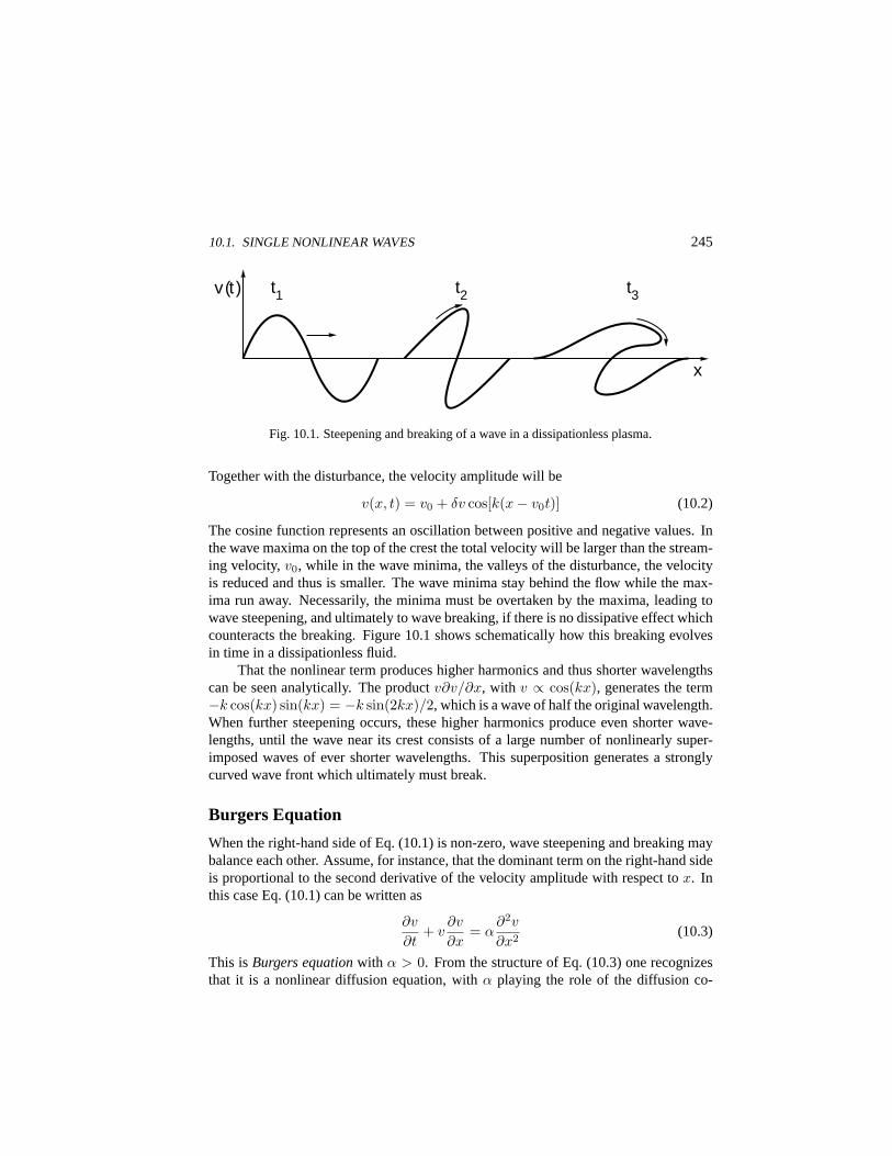
10.1. SINGLE NONLINEAR WAVES 245
t2 t1 t3 v (t )
x
Fig. 10.1. Steepening and breaking of a wave in a dissipationless plasma.
Together with the disturbance, the velocity amplitude will be
v(x, t) = v0 + δv cos[k(x− v0t)] (10.2)
The cosine function represents an oscillation between positive and negative values. Inthe wave maxima on the top of the crest the total velocity will be larger than the stream-ing velocity,v0, while in the wave minima, the valleys of the disturbance, the velocityis reduced and thus is smaller. The wave minima stay behind the flow while the max-ima run away. Necessarily, the minima must be overtaken by the maxima, leading towave steepening, and ultimately to wave breaking, if there is no dissipative effect whichcounteracts the breaking. Figure 10.1 shows schematically how this breaking evolvesin time in a dissipationless fluid.
That the nonlinear term produces higher harmonics and thus shorter wavelengthscan be seen analytically. The productv∂v/∂x, with v ∝ cos(kx), generates the term−k cos(kx) sin(kx) = −k sin(2kx)/2, which is a wave of half the original wavelength.When further steepening occurs, these higher harmonics produce even shorter wave-lengths, until the wave near its crest consists of a large number of nonlinearly super-imposed waves of ever shorter wavelengths. This superposition generates a stronglycurved wave front which ultimately must break.
Burgers Equation
When the right-hand side of Eq. (10.1) is non-zero, wave steepening and breaking maybalance each other. Assume, for instance, that the dominant term on the right-hand sideis proportional to the second derivative of the velocity amplitude with respect tox. Inthis case Eq. (10.1) can be written as
∂v
∂t+ v
∂v
∂x= α
∂2v
∂x2(10.3)
This isBurgers equationwith α > 0. From the structure of Eq. (10.3) one recognizesthat it is a nonlinear diffusion equation, withα playing the role of the diffusion co-

246 10. NONLINEAR WAVES
v (x ) v (−∞)
v (∞)
Fig. 10.2. Shock ramp solution of Burgers dissipative equation.
efficient and the convective term providing the nonlinearity. However, in comparisonwith a linear diffusion equation lacking the nonlinear term the character of the solutionschange totally. The reason is that the diffusive second order derivative may compensatefor the nonlinearity. For increasing nonlinear steepening the second derivative startscontributing more and more until it becomes comparable to the nonlinear term and thesteepening ceases. In this state the solution is stationary with vanishing time derivative.
The stationary solution can be found when transforming to a coordinate systemmoving with the wave. Let the velocity of the wave beu and introduce the new coordi-nate,y = x− ut, Burgers equation is written
α∂2v
∂y2= (v − u)
∂v
∂y(10.4)
We are only interested in localized solutions which are regular at infinity. The solutionobtained is
v − u = −u tanh[u(x− ut)/2α] (10.5)
The form of this solution is ashock ramp. Figure 10.2 shows the form of the shockramp as solution of Burgers equation. The height of the ramp isu, the thickness ofthe ramp isα/u, and the shock propagates with velocityu alongx. Hence, Burgersequation yields as stationary solutions propagating shock waves where the dissipationcontained in the diffusion coefficient becomes effective in the steep gradient inside theramp where it balances the nonlinearity.
Korteweg-de Vries Equation
Balancing the nonlinearity with the help of dissipation is only one possibility. Whenthere is no dissipation in the medium, the right-hand side of Eq. (10.1) may contain a

10.1. SINGLE NONLINEAR WAVES 247
third-order derivative with respect tox. Third-order spatial derivatives describe disper-sion. The equation obtained is theKorteweg-de Vries equation
∂v
∂t+ v
∂v
∂x+ β
∂3v
∂x3= 0 (10.6)
The simplest way to understand the origin of nonlinear equations of the type of theBurgers and the Korteweg-de Vries equations is to consider the general one-dimensionaldispersion relation,ω(k) = 0, where the frequency is an arbitrary function of thewavenumber. With a Taylor expansion of the frequency with respect tok we get
ω(k) = ω(0) + vgrk +12
∂2ω
∂k2k2 +
16
∂3ω
∂k3k3 + . . . (10.7)
If we now interpret frequency and wavenumber as one-dimensional operators
ω = i∂/∂t
k = −i∂/∂x(10.8)
acting on the wave function,ψ(x, t), it is easy to see that the terms up to the third-orderderivative just reconstitute an equation which contains both the Burgers and Korteweg-de Vries equations. In such an approach one can ignore the linear term in the aboveexpansion of the frequency, because this term describes only a Doppler shift. Hence,all discussion which follows refers to a frame of reference which moves at the constantgroup velocity,vgr.
The coefficients in front of the operators are derivatives of the frequency withrespect to wavenumber. It is the frequency which contains all information about thenonlinear evolution of the system. This can be understood by analogy to quantum me-chanics when one recognizes that the frequency is the energy and, hence, plays the roleof the Hamiltonian of the system in which all the information is stored. Burgers equa-tion is obtained when cutting the expansion after the second derivative term, while theKorteweg-de Vries equation follows when dropping the second derivative but keepingthe third-order derivative ofω(k).
Similar to Burgers equation, the Korteweg-de Vries equation also allows for sta-tionary localized solutions. But because dispersion causes only reversible effects, sucha solution will be restricted to a finite spatial interval. Assume that it exists and movesat speedu. Again introducing the coordinatey = x− ut, measured from the center ofthe localized solution, the Korteweg-de Vries equation (10.6) can be transformed intothe third-order ordinary differential equation
(v − u)∂v
∂y+ β
∂3v
∂y3= 0 (10.9)
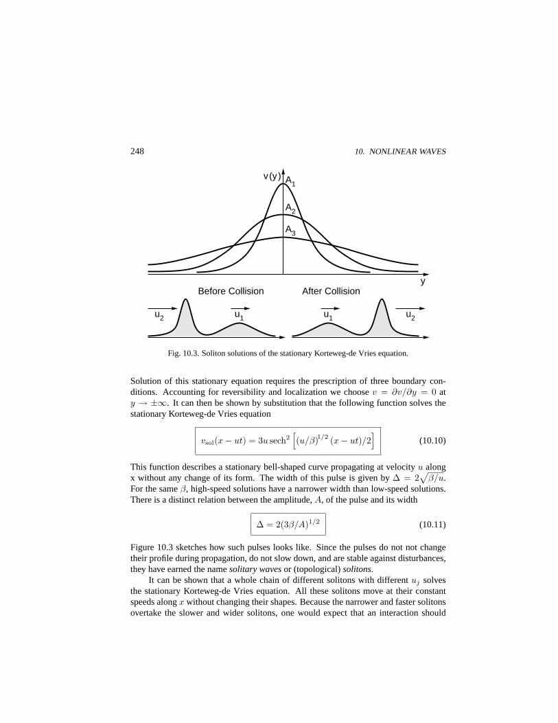
248 10. NONLINEAR WAVES
v (y ) A1
A2
A3
y
u2
Before Collision After Collision
u1 u1 u2
Fig. 10.3. Soliton solutions of the stationary Korteweg-de Vries equation.
Solution of this stationary equation requires the prescription of three boundary con-ditions. Accounting for reversibility and localization we choosev = ∂v/∂y = 0 aty → ±∞. It can then be shown by substitution that the following function solves thestationary Korteweg-de Vries equation
vsol(x− ut) = 3u sech2[(u/β)1/2 (x− ut)/2
](10.10)
This function describes a stationary bell-shaped curve propagating at velocityu alongx without any change of its form. The width of this pulse is given by∆ = 2
√β/u.
For the sameβ, high-speed solutions have a narrower width than low-speed solutions.There is a distinct relation between the amplitude,A, of the pulse and its width
∆ = 2(3β/A)1/2 (10.11)
Figure 10.3 sketches how such pulses looks like. Since the pulses do not not changetheir profile during propagation, do not slow down, and are stable against disturbances,they have earned the namesolitary wavesor (topological)solitons.
It can be shown that a whole chain of different solitons with differentuj solvesthe stationary Korteweg-de Vries equation. All these solitons move at their constantspeeds alongx without changing their shapes. Because the narrower and faster solitonsovertake the slower and wider solitons, one would expect that an interaction should

10.1. SINGLE NONLINEAR WAVES 249
occur. But calculations and numerical experiments show that collisions between two ormore solitons have practically now effect on the solitons. After collision they reappearand separate at their initial speeds as sketched in the lower part of Fig. 10.3.
This behavior is characteristic for topological solitons and stationary structures.In systems described by equations of the same family as the Korteweg-de Vries equa-tion, characterized by dispersion effects only, topological solitons constitute a naturalfundamental eigenmode system of waves. On the other hand, when a wave evolvesinto a chain of solitons of different amplitudes, widths and speeds, the plasma assumesa grainy quasi-irregular structure, which cannot be described anymore by weak turbu-lence theory. This is the origin of the notion that the soliton state of a plasma corre-sponds to the state ofstrong plasma turbulence. In this state the plasma is filled withlocalized waves and assumes the character of a gas of particles with the solitons con-stituting the particles of different speeds, momenta and energies. One possibility todescribe such a strongly turbulent state would thus be a kinetic quasi-particle descrip-tion with the particles being solitons.
Stationary Solution of the Korteweg-de Vries Equation
We have guessed the solution of the stationary Korteweg-de Vries equation. Let usnow demonstrate, how this solution is found. Equation (10.9) can be directly integratedonce. Applying the boundary conditions at infinity, the integration constant turns out tobe zero yielding the result
β∂2v
∂y2= v(u− 1
2v) (10.12)
Inspection of this equation shows immediately that it is of the type of the equation ofmotion of a pseudo-particle with the left-hand side the acceleration,β the mass, andthe right-hand side the force. Such an equation can be solved by multiplying it with thepseudo-velocity,∂v/∂y. The right-hand side can be represented as the derivative of apseudo-potentialor Sagdeev potential, S(v). Integrating once more and again applyingthe boundary conditions at infinity gives the pseudo-energy conservation law
β
2
(∂v
∂y
)2
=v2
2
(u− 1
3v
)= −S(v) (10.13)
This equation allows for a first conclusion. Because the left-hand side is a positivequantity, solutions exist only under the condition that the pseudo-potential is negative
S(v) =v2
2
(13v − u
)< 0 (10.14)
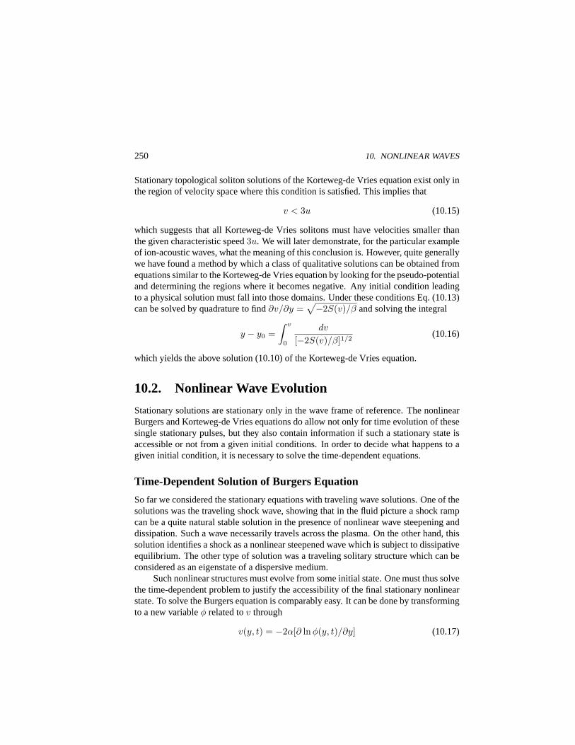
250 10. NONLINEAR WAVES
Stationary topological soliton solutions of the Korteweg-de Vries equation exist only inthe region of velocity space where this condition is satisfied. This implies that
v < 3u (10.15)
which suggests that all Korteweg-de Vries solitons must have velocities smaller thanthe given characteristic speed3u. We will later demonstrate, for the particular exampleof ion-acoustic waves, what the meaning of this conclusion is. However, quite generallywe have found a method by which a class of qualitative solutions can be obtained fromequations similar to the Korteweg-de Vries equation by looking for the pseudo-potentialand determining the regions where it becomes negative. Any initial condition leadingto a physical solution must fall into those domains. Under these conditions Eq. (10.13)can be solved by quadrature to find∂v/∂y =
√−2S(v)/β and solving the integral
y − y0 =∫ v
0
dv
[−2S(v)/β]1/2(10.16)
which yields the above solution (10.10) of the Korteweg-de Vries equation.
10.2. Nonlinear Wave Evolution
Stationary solutions are stationary only in the wave frame of reference. The nonlinearBurgers and Korteweg-de Vries equations do allow not only for time evolution of thesesingle stationary pulses, but they also contain information if such a stationary state isaccessible or not from a given initial conditions. In order to decide what happens to agiven initial condition, it is necessary to solve the time-dependent equations.
Time-Dependent Solution of Burgers Equation
So far we considered the stationary equations with traveling wave solutions. One of thesolutions was the traveling shock wave, showing that in the fluid picture a shock rampcan be a quite natural stable solution in the presence of nonlinear wave steepening anddissipation. Such a wave necessarily travels across the plasma. On the other hand, thissolution identifies a shock as a nonlinear steepened wave which is subject to dissipativeequilibrium. The other type of solution was a traveling solitary structure which can beconsidered as an eigenstate of a dispersive medium.
Such nonlinear structures must evolve from some initial state. One must thus solvethe time-dependent problem to justify the accessibility of the final stationary nonlinearstate. To solve the Burgers equation is comparably easy. It can be done by transformingto a new variableφ related tov through
v(y, t) = −2α[∂ ln φ(y, t)/∂y] (10.17)
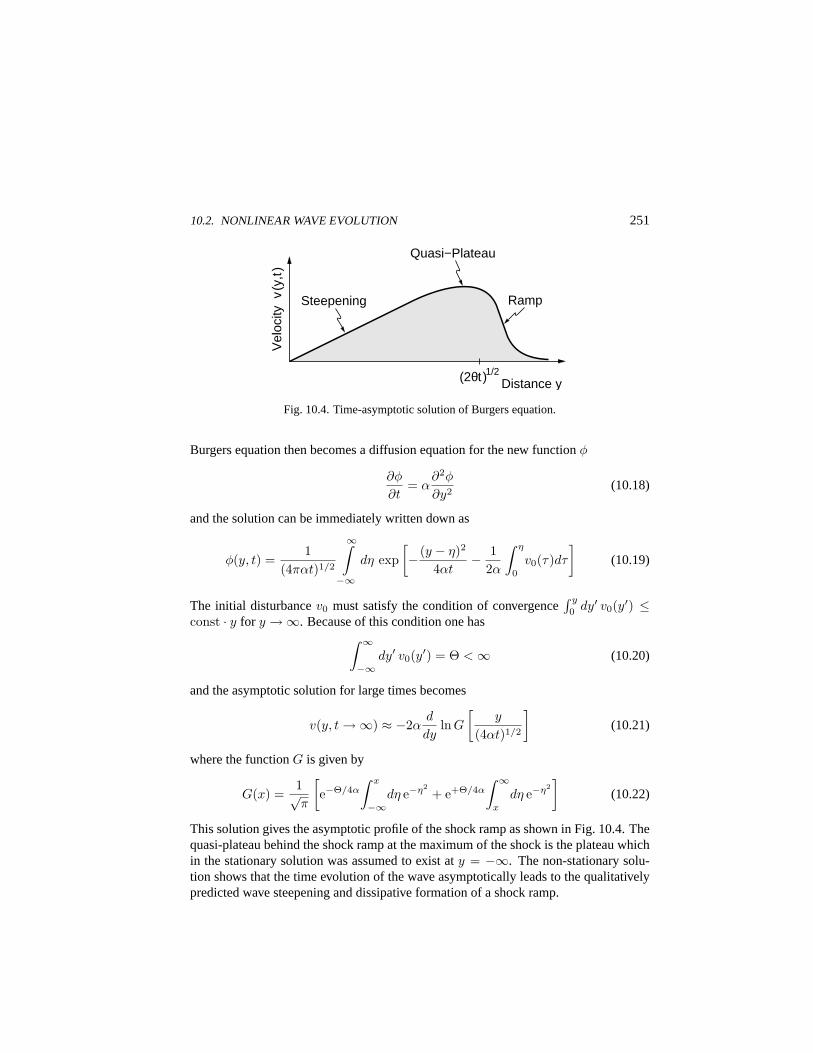
10.2. NONLINEAR WAVE EVOLUTION 251
(2θt )1/2
Steepening
Quasi−Plateau
Ramp
Distance y
Vel
ocity
v(y
,t)
Fig. 10.4. Time-asymptotic solution of Burgers equation.
Burgers equation then becomes a diffusion equation for the new functionφ
∂φ
∂t= α
∂2φ
∂y2(10.18)
and the solution can be immediately written down as
φ(y, t) =1
(4παt)1/2
∞∫
−∞dη exp
[− (y − η)2
4αt− 1
2α
∫ η
0
v0(τ)dτ
](10.19)
The initial disturbancev0 must satisfy the condition of convergence∫ y
0dy′ v0(y′) ≤
const · y for y →∞. Because of this condition one has∫ ∞
−∞dy′ v0(y′) = Θ < ∞ (10.20)
and the asymptotic solution for large times becomes
v(y, t →∞) ≈ −2αd
dyln G
[y
(4αt)1/2
](10.21)
where the functionG is given by
G(x) =1√π
[e−Θ/4α
∫ x
−∞dη e−η2
+ e+Θ/4α
∫ ∞
x
dη e−η2]
(10.22)
This solution gives the asymptotic profile of the shock ramp as shown in Fig. 10.4. Thequasi-plateau behind the shock ramp at the maximum of the shock is the plateau whichin the stationary solution was assumed to exist aty = −∞. The non-stationary solu-tion shows that the time evolution of the wave asymptotically leads to the qualitativelypredicted wave steepening and dissipative formation of a shock ramp.
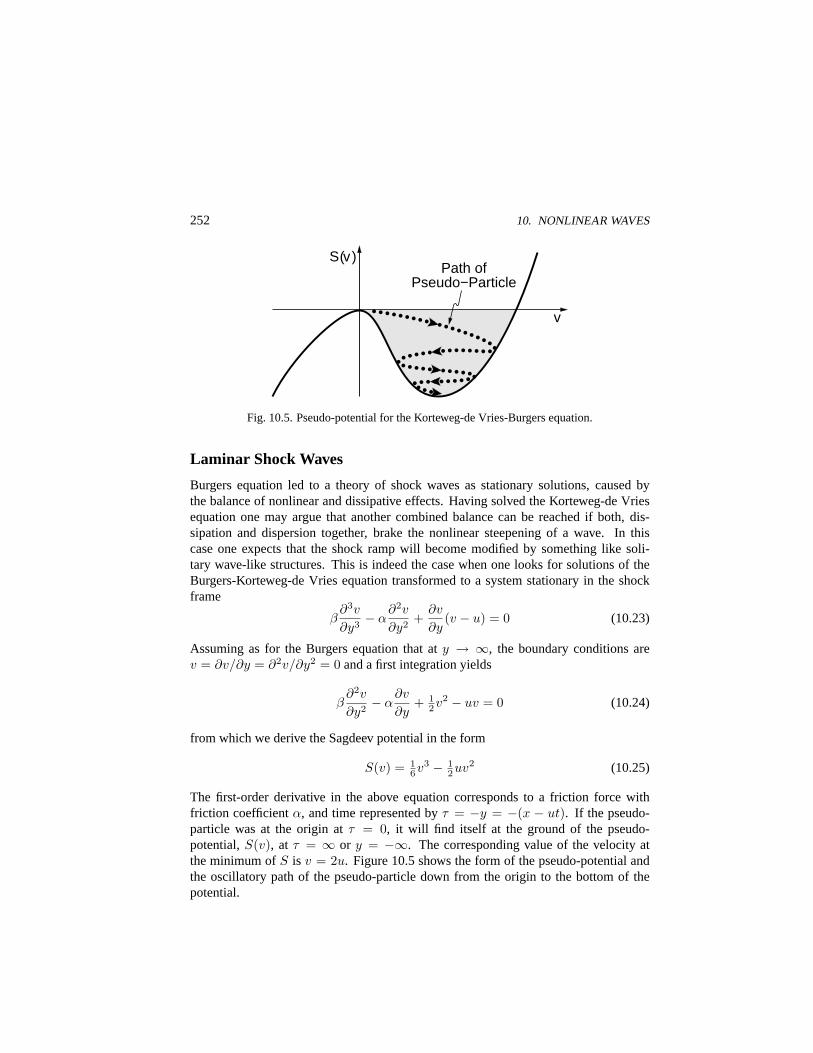
252 10. NONLINEAR WAVES
Path of Pseudo−Particle
S(v )
v
Fig. 10.5. Pseudo-potential for the Korteweg-de Vries-Burgers equation.
Laminar Shock Waves
Burgers equation led to a theory of shock waves as stationary solutions, caused bythe balance of nonlinear and dissipative effects. Having solved the Korteweg-de Vriesequation one may argue that another combined balance can be reached if both, dis-sipation and dispersion together, brake the nonlinear steepening of a wave. In thiscase one expects that the shock ramp will become modified by something like soli-tary wave-like structures. This is indeed the case when one looks for solutions of theBurgers-Korteweg-de Vries equation transformed to a system stationary in the shockframe
β∂3v
∂y3− α
∂2v
∂y2+
∂v
∂y(v − u) = 0 (10.23)
Assuming as for the Burgers equation that aty → ∞, the boundary conditions arev = ∂v/∂y = ∂2v/∂y2 = 0 and a first integration yields
β∂2v
∂y2− α
∂v
∂y+ 1
2v2 − uv = 0 (10.24)
from which we derive the Sagdeev potential in the form
S(v) = 16v3 − 1
2uv2 (10.25)
The first-order derivative in the above equation corresponds to a friction force withfriction coefficientα, and time represented byτ = −y = −(x − ut). If the pseudo-particle was at the origin atτ = 0, it will find itself at the ground of the pseudo-potential,S(v), at τ = ∞ or y = −∞. The corresponding value of the velocity atthe minimum ofS is v = 2u. Figure 10.5 shows the form of the pseudo-potential andthe oscillatory path of the pseudo-particle down from the origin to the bottom of thepotential.
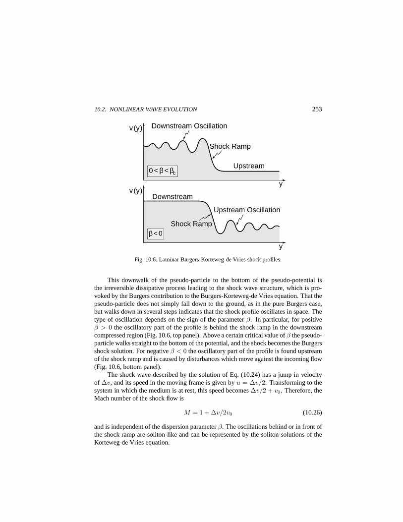
10.2. NONLINEAR WAVE EVOLUTION 253
v (y)
y v (y)
y
Downstream Oscillation
Downstream
Upstream Oscillation
Shock Ramp
Shock Ramp
Upstream 0 < β < βc
β < 0
Fig. 10.6. Laminar Burgers-Korteweg-de Vries shock profiles.
This downwalk of the pseudo-particle to the bottom of the pseudo-potential isthe irreversible dissipative process leading to the shock wave structure, which is pro-voked by the Burgers contribution to the Burgers-Korteweg-de Vries equation. That thepseudo-particle does not simply fall down to the ground, as in the pure Burgers case,but walks down in several steps indicates that the shock profile oscillates in space. Thetype of oscillation depends on the sign of the parameterβ. In particular, for positiveβ > 0 the oscillatory part of the profile is behind the shock ramp in the downstreamcompressed region (Fig. 10.6, top panel). Above a certain critical value ofβ the pseudo-particle walks straight to the bottom of the potential, and the shock becomes the Burgersshock solution. For negativeβ < 0 the oscillatory part of the profile is found upstreamof the shock ramp and is caused by disturbances which move against the incoming flow(Fig. 10.6, bottom panel).
The shock wave described by the solution of Eq. (10.24) has a jump in velocityof ∆v, and its speed in the moving frame is given byu = ∆v/2. Transforming to thesystem in which the medium is at rest, this speed becomes∆v/2 + v0. Therefore, theMach number of the shock flow is
M = 1 + ∆v/2v0 (10.26)
and is independent of the dispersion parameterβ. The oscillations behind or in front ofthe shock ramp are soliton-like and can be represented by the soliton solutions of theKorteweg-de Vries equation.
254 10. NONLINEAR WAVES
Invariants of Korteweg-de Vries’ Equation
Solving the time-dependent Korteweg-de Vries equation requires considerably moreeffort. Before discussing the general method, we demonstrate that the Korteweg-deVries equation has a large number of invariants
In =∫ ∞
−∞Nn(x, t) dx (10.27)
where the generalized number densities,Nn, and generalized momentum flux densities,Pn, satisfy the following one-dimensional conservation laws
∂Nn/∂t +∇xPn = 0 for n = 1, 2, 3 . . . (10.28)
The Korteweg-de Vries equation can be written as a conservation law forn = 1
∂v/∂t +∇x
(12v2 + β∇2
xv)
= 0 (10.29)
The generalized first-order number density is the velocity itself, while the first-ordermomentum flux density is defined as the term in brackets, identifying the Korteweg-de Vries equation as the conservation law of the generalized momentum
∫v(x, t) dx.
The higher-order conservation laws can be obtained by successive multiplication of theKorteweg-de Vries equation byv, v2, . . . The next conservation law is
12
∂v2
∂t= −∇x
[v3
3+ β
(v∇2
xv − 12∇2
xv
)](10.30)
This equation corresponds to an energy conservation law. The other higher-order con-servation laws have no direct physical interpretation. The point is that the Korteweg-deVries equation functions similar to a kinetic equation. It is the basic equation of ahierarchy of conservation laws, which can be derived as moment equations in a waysimilar to the derivation of moment equations for the hydrodynamic variables from theLiouville equation.
It can be shown that thenth order ‘density’ invariants can be represented as poly-nomials inv,∇xv when expanding with respect to the small dispersion parameter,β
Nn = vn/n− 12 (n− 1)(n− 2)βvn−3(∇xv)2 + O(β2) (10.31)
For the Korteweg-de Vries soliton (10.10) the solution forv is given, and the invariantscan be calculated explicitly
In,sol =∫ ∞
−∞dxNn[vsol] = (12β)1/2(3u)(n−1/2)2n[(n− 1)!]2/(2n− 1)! (10.32)
These invariants play a central role in the time-dependent solution of the Korteweg-deVries equation.
10.3. INVERSE-SCATTERING METHOD 255
10.3. Inverse-Scattering Method
In this section we present one very general method of solving time-dependent nonlinearequations, which applies to a whole class of equations. We use this method for solvingthe Korteweg-de Vries equation.
Inverse-Scattering Solution of Korteweg-de Vries Equation
It is quite simple to solve the linearized Korteweg-de Vries equation and to guess itsstationary nonlinear condition, but it is much more involved to find analytical time-de-pendent solutions of the nonlinear equation. The idea of the method is as follows. Inquantum mechanics the Schrodinger equation describes the energy states of a systemexposed to an external potential. Knowing the full spectrum of these states it is possi-ble to perfectly reconstruct this external potential by solving a particular GLM-integralequation given by Gelfand, Levitan and Marchenko. Assuming that this potential isthe unknown solution of the Korteweg-de Vries equation and using the well-knownmethods of solving the Schrodinger equation and the GLM-equation, together with theknowledge of the initial condition and the form of the above invariants, the solutionof the Korteweg-de Vries equation can be constructed. This way of solving nonlin-ear equations is calledinverse scattering method, because the inverse problem of theSchrodinger equation arises in the investigation of light-scattering problems in astro-physics.
In order to sketch how this method works, consider Schrodinger’s equation for thewave function,ψ(x, t), in the particular form
∇2xψ + 1
6 [λ(t)− v(x, t)] ψ = 0 (10.33)
The factor 1/6 has been extracted for convenience. The potentialv(x, t) is chosen asthe unknown function in the time-dependent KdV-equation. The Schrodinger equationis assumed to be stationary and depends on time only via the time dependence ofvand the corresponding time dependence of the energy eigenvalues,λ. Thus the timedependence is only parametric and determined by the conditions onv
∂v
∂t+ v∇xv +∇3
xv = 0 (10.34)
which is the Korteweg-de Vries equation withβ = 1, andv(x, 0) = 0 at x → ±∞.Note that the solutions of the Korteweg-de Vries equation are reversible. The choice ofβ corresponds to the following rescaling:v → β1/5v, t → β1/5t, x → β2/5x. Insertingv from (10.33) into (10.34) gives
∇x
(ψ∇x −∇xψ)
[∂ψ
∂t− 1
2(v + λ)∇xψ +∇3
xψ
]= −6ψ2 ∂λ
∂t(10.35)
256 10. NONLINEAR WAVES
The left-hand side of this expression is a divergence which, when integrating over allspace and taking into account that the solution of the Korteweg-de Vries equation andthus also that of the Schrodinger equation is bounded, must vanish. Hence, the eigen-values of the discrete spectrum of the Schrodinger equation must be time-independent,wheneverv is a solution of the Korteweg-de Vries equation,∂λ/∂t = 0. Consequently,one finds by integrating the last equation twice that the wave function satisfies the con-dition
∂ψ
∂t− 1
2(v + λ)∇xψ +∇3
xψ = ψ
(A + B
∫dxψ2
)(10.36)
The coefficientsA,B vanish for the discrete spectrum, since in the limitx → ±∞the left-hand side must vanish and because of the normalization condition of the wavefunction. In the case of a continuous spectrum one must, however, take into accountthat a wave can fall in from infinity. In this caseA,B 6= 0.
In the discrete part of the spectrumψ is represented as the expansion with respectto eigenfunctions,ψn, of the Schrodinger equation in the Hilbert space representation.These eigenfunctions must be regular forx → ±∞, such that
ψn(x, t) ≈ cn±(t) exp(∓knx) for x → ±∞ (10.37)
where the spatial decay decrement isk2n = −λn/6. In order to find the coefficients,
one inserts this asymptotic expression into the above condition onψ and finds
cn±(t) = cn±(0) exp(±4k3nt) (10.38)
Similarly, the regular eigenfunctions of the continuous spectrum may be chosen as
ψcont ≈ c±(k, t) exp(±ikx) + δ∓ exp(−ikx) for x → ±∞ (10.39)
Hereδ+ = 1 andδ− = 0. Again inserting into Eq. (10.36) allows to determine thecoefficients of the continuous spectrum asB = 0, A = 4ik3, and one finds
c+(k, t) = c+(k, 0) exp(4ik3t)c−(k, t) = c−(k, 0)
(10.40)
Clearly,c+ is the reflection coefficient, whilec− is the transmission coefficient of thewave incident fromx = +∞, and we must have in addition
|c−|2 + |c+|2 = 1 (10.41)
The former expressions show that the time dependence of the coefficientscn andc isentirely determined by the spectrum. One has to find only the initial coefficients att = 0. This can be done by solving the time independent Schrodinger equation using
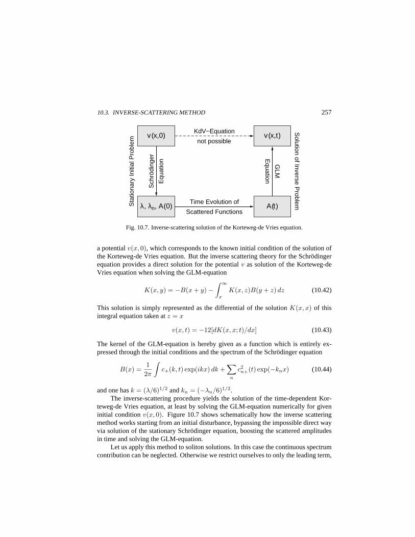
10.3. INVERSE-SCATTERING METHOD 257
v (x,0) v (x,t) KdV−Equation
λ, λn, A(0) A(t)
not possible
Time Evolution of
Scattered Functions
Sta
tiona
ry In
itial
Pro
blem
Solution of Inverse P
roblem
Sch
rödi
nger
Equ
atio
n GLM
Equation
Fig. 10.7. Inverse-scattering solution of the Korteweg-de Vries equation.
a potentialv(x, 0), which corresponds to the known initial condition of the solution ofthe Korteweg-de Vries equation. But the inverse scattering theory for the Schrodingerequation provides a direct solution for the potentialv as solution of the Korteweg-deVries equation when solving the GLM-equation
K(x, y) = −B(x + y)−∫ ∞
x
K(x, z)B(y + z) dz (10.42)
This solution is simply represented as the differential of the solutionK(x, x) of thisintegral equation taken atz = x
v(x, t) = −12[dK(x, x; t)/dx] (10.43)
The kernel of the GLM-equation is hereby given as a function which is entirely ex-pressed through the initial conditions and the spectrum of the Schrodinger equation
B(x) =12π
∫c+(k, t) exp(ikx) dk +
∑n
c2n+(t) exp(−knx) (10.44)
and one hask = (λ/6)1/2 andkn = (−λn/6)1/2.The inverse-scattering procedure yields the solution of the time-dependent Kor-
teweg-de Vries equation, at least by solving the GLM-equation numerically for giveninitial condition v(x, 0). Figure 10.7 shows schematically how the inverse scatteringmethod works starting from an initial disturbance, bypassing the impossible direct wayvia solution of the stationary Schrodinger equation, boosting the scattered amplitudesin time and solving the GLM-equation.
Let us apply this method to soliton solutions. In this case the continuous spectrumcontribution can be neglected. Otherwise we restrict ourselves to only the leading term,
258 10. NONLINEAR WAVES
n = 1, in the sum in the functionB(x). This allows to write asymptotically
B(x, t) = c21(0) exp(8k3
1t− k1x) (10.45)
where we used the fact that asymptoticallyx ≈ 8k21t. With this expression the GLM-
equation gives
K(x, y; t) = −c21(0)
exp[−k1(x + y) + 8k3
1t]
1 + [c21(0)/2k1] exp [−2k1x + 8k3
1t](10.46)
which, when inserted in the prescription of obtaining the solution of the Korteweg-deVries equation from the derivative ofK, yields the soliton solution
v(x, t) = −12k21 sech2
[k1(x− x0)− 4k2
1t]
(10.47)
with c21(0) = 2k1 exp(2k1x0). The amplitude of the soliton is now12k2
1, and its veloc-ity one third of this, which coincides with the solution found earlier.
Self-Similar Solution
Let us return to the Korteweg-de Vries equation (10.34) and write the initial conditionv(x, 0) = uφ(x/`) such that the functionφ describes the self-similar shape of thesolution,ξ = x/` is a dimensionless coordinate, and` is the characteristic width ofthe localized solution which for the soliton solutionvsol is ` = (4β/u)1/2. It is thenpossible to rewrite the Schrodinger equation
ψ′′(ξ) + 16σ2[Wn + φ(ξ)]ψ(ξ) = 0 (10.48)
where the double prime denotes the second spatial derivative, and the quantityσ2 =u`2/β serves as a parameter. The amplitudes,cn, of the soliton solutions of the Korte-weg-de Vries equation are related to the energy eigenvalues of the Schrodinger equation
cn = −2uWn (10.49)
The structure of the Schrodinger equation then shows that forφ(ξ) < 0 no discretespectrum and therefore no solitons exist. Initial disturbances of this kind do not evolveinto localized solutions. The discrete spectrum requires that
Φ =∫
φ(ξ) dξ > 0 (10.50)
and the number of solitons which evolve depends on the value of the similarity parame-ter,σ, such that for smallσ only one eigenvalue and thus one soliton exists. This valueis found by a lengthy perturbation calculation
W1 = −(σ2/24)Φ2 for σ2 ¿ 12 = σ2sol (10.51)
10.3. INVERSE-SCATTERING METHOD 259
and the amplitude of this solitons can be represented through
c1 = 2uΦ (10.52)
The quantityσsol is the similarity parameter for the stationary soliton solution. Thisimplies that under non-stationary conditions an initial disturbance will decay into manysolitons of small amplitude. From this consideration it becomes clear that for large val-ues ofσ the number of solitons which evolve from a given initial disturbance becomeslarge by itself. The nature of the Korteweg-de Vries equation is thus to split a givenlarge initial disturbance into a large number of small-amplitude nonlinear structureswhich, after formation, behave as independent non-interacting entities, while giving theplasma a grainy texture which we call strong turbulence. The large-amplitude singlesoliton found under stationary conditions is thus an idealized solution, which probablydoes not exist when evolving from an initial condition.
Soliton Distribution
In the case of large initial disturbances it is possible to calculate the number of solitonswhich evolve out of the disturbance. This number can be estimated using the infinite setof invariants of the Korteweg-de Vries equation. Because the amplitudes of the evolv-ing solitons are determined by these invariants and are not equally large, one can finda distribution function of soliton amplitudes or, because the amplitudes are unambigu-ously related to the soliton speeds, a distribution function of the solitons with respect totheir velocities. The numberdN of solitons with amplitudes in the interval[u, u + du]can be defined as
dN = F (u) du (10.53)
On the other hand, the density of energy levels of the Schrodinger equation in the dis-crete spectrum is given as
dN
dW=
σ√24π
∫dξ
[φ(ξ)−W ]1/2(10.54)
in the region of positive initial disturbance,φ > 0. These two expressions enable oneto find the distribution functionF (u) of the soliton amplitudes
F (u) =σ
4π(3u0)1/2
∫dξ [2u0φ(ξ)− 3u]−1/2 (10.55)
The integration is to be taken over the positive part of the argument of the square root,2u0φ > 3u. The lengthy derivation is not given here. Integrating from zero to infinityone can find the number of solitons
N =∫
F (u)du =σ√6π
∫dξ φ1/2(ξ) (10.56)

260 10. NONLINEAR WAVES
These equations can serve to estimate the graininess of a Korteweg-de Vries turbulentplasma. They also play a role in more general theories of strong plasma turbulencecaused by drift waves and electron acoustic waves.
10.4. Acoustic Solitons
To obtain nonlinear equations governing the evolution of plasma waves, it is necessaryto reduce the full set of complicated nonlinear equations of plasma physics which can-not be solved by analytical methods to one of the nonlinear equations derived in theprevious sections. This can in general not be done, but there are a number of caseswhen it is possible to apply some reduction methods which lead to the Korteweg-deVries or Burgers equations. In this section we show how this reduction method worksfor a ion-acoustic, electron-acoustic, and kinetic Alfven waves.
Reductive Perturbation Method
Both the Burgers and Korteweg-de Vries equations are general equations which do notapply exclusively to plasmas. As a first example of solitons in a plasma we considernonlinear ion-acoustic waves in the two-fluid approximation. This means that we arenot interested in the instability causing these waves, but assume that an ion-acousticwave exists in the plasma and that this wave undergoes nonlinear evolution. Whatthen is the dynamics of this evolution and which of the nonlinear equations governsit? Hence, we are interested in reducing the full nonlinear set of two-fluid equationsto one master equation, which describes nonlinear ion-acoustic waves. The general re-duction scheme of finding such a reduced equation is the reductive method of stretchedcoordinates.
Consider the invariance of the Korteweg-de Vries equation with respect to thefollowing coordinate transformations
t → εt x → ε1/3x v → ε−2/3v (10.57)
All its solutions have the same shape if transformed accordingly and are calledself-similar. They can be written
v(x, t) = β(3βt)−2/3ψ[x/(3βt)1/3] (10.58)
A transformation of this kind is called aself-similarity transformation. A self-similaritytransformation can also be found for the Burgers equation. It can be applied to reducea system of partial differential equations of the kind for the column vector,U
∂U∂t
+ A · ∇xU +q∑
µ=1
p∏ν=1
(Hν
µ
∂U∂t
+ Kνµ∇xU
)= 0 (10.59)
10.4. ACOUSTIC SOLITONS 261
with Hνµ , Kν
µ matrices which themselves depend onU, to a simpler nonlinear equation.One introduces a small parameterε ¿ 1 and expands
U = U0 + εU1 + . . . (10.60)
while at the same time introducing the stretched coordinates
ξ = εa(x− ut) τ = εa+1t (10.61)
wherea = (p − 1)−1. If we now require thatU1 → 0 for x → ∞, write U1 = Rφ,and chose the equation which determines the column eigenvector,R, from the matrixequation
(A − uI) ·R = 0 (10.62)
we can reduce the above very complicated system asymptotically to the simpler self-similar equation forφ
∂φ
∂τ+ αφ∇ξφ + β∇p
ξφ = 0 (10.63)
This equation is a nonlinear dispersive equation with a dispersion of orderp. Its coeffi-cients can be expressed through the velocityu andR. β is the solution of the dispersionrelation of the linear system
ω = uk + ip−1βkp + . . . (10.64)
andα = ∇u · (u0R0). Here we used that the wavenumberk = O(εp) is of orderp.
Ion-Acoustic Solitons
The first example of solitons relevant for space plasmas are acoustic solitons. We con-sider a one-dimensional system in which ion-acoustic waves have been excited by,for example, a field-aligned current instability. In the one-dimensional field-alignedcase the physics is independent of the magnetic field. Normalizing all quantities,nj →nj/n0, vj → vj/cia, E→ eE/(mekBTe)1/2ωpe (or φ→ eφ/kBTe), x→ x/λD,andt→ωpit, and assuming Boltzmann-distributed electrons, the equations describingthe evolution of the plasma are
∂ni
∂t+
∂(nivi)∂x
= 0
∂vi
∂t+ vi
∂vi
∂x= −∂φ
∂x(10.65)
∂2φ
∂x2= −ni + exp(φ)
262 10. NONLINEAR WAVES
When linearizing these equations one obtains the dispersion relation
ω2 = k2/(1 + k2) (10.66)
which in the small wavenumber limit,k2 ¿ 1, can be expanded and reduced to
ω = k(1− k2/2) (10.67)
One immediately recognizes that the dispersion coefficient will have the value|β| =1/2. We now assume initial quasineutrality,ni = ne, and rewrite the equation ofmotion as
∂vi
∂t+ vi
∂vi
∂x= − 1
ni
∂ni
∂x(10.68)
This equation is identical with the momentum conservation equation of a gas with soundvelocity cia = 1, in which the electrons exert a pressure on the plasma through theelectric field,E = −∇xφ. Therefore the nonlinear wave is an ion-acoustic wave. Butwhen the wave steepens, the left-hand side of the Poisson equation,∇2
xφ, grows dueto inertial effects of the steepening gradients, and quasineutrality becomes obsolete.This causes the dispersive effects in the dispersion relation, which ultimately lead tostabilization of the nonlinear steepening. One therefore expects that ion-acoustic wavesmay lead to the formation of topological solitons.
Let us look for a solution of the above nonlinear equations, which depends onx, tin the formξ = x − ut, and let us further assume homogeneous boundary conditionsfor |ξ|→∞, i.e.,ni→1, vi = φ = ∇ξφ→0. Then we get
12 (∇ξφ)2 = exp(φ) + u(u2 − 2φ)1/2 − (u2 + 1) (10.69)
Setting the left-hand side of this expression to zero and assuming that the potential hasan extremum,φmax, at the place where its derivative vanishes, we obtain for the speedof the structure
u2 =[exp φmax − 1]2
2[expφmax − 1− φmax](10.70)
Further assuming thatφmax ¿ 1, andu− 1 = δu ¿ 1, one gets
(∇ξφ)2 = 23φ2(3δu− φ) = −S(φ) (10.71)
where the right-hand side is the pseudo-potential of the ion-acoustic wave. We imme-diately identify this equation as the first integral of the stationary Korteweg-de Vriesequation. The solution is the Korteweg-de Vries soliton
φ = 3δu sech2
[(δu
2
)1/2
(x− ut)
](10.72)
10.4. ACOUSTIC SOLITONS 263
which is valid for small-amplitude slow ion-acoustic solitons. The maximum amplitudeof the soliton is given by the condition that the pseudo-potential must be negative forsolitons to occur. One finds thatφmax = u2/2. Inserting for the speed into Eq. (10.70)yields φmax ≈ 1.3 and therefore as the maximum speed of the solitonumax ≈ 1.6.Since this speed is normalized to the ion-acoustic velocity, we find that ion-acousticsolitons exist for Mach numbers
Mia,sol < 1.6 (10.73)
The stationary solution obtained is, of course, not the full story because the systemmust evolve toward the state where the soliton has formed. We now apply the reductiveperturbation method to the initial system of equations describing the nonlinear evolutionof ion-acoustic waves in order to find the basic nonlinear equation. Eliminating the iondensity and electric field from the equations, the system is reduced to the following twoequations
∂ne
∂t+∇x(nevi)−∇x
[(∂
∂t+ vi∇x
)∇x ln ne
]= 0 (10.74)
∂vi
∂t+ vi∇xvi +∇x ln ne = 0 (10.75)
From this equation we read thatp = 3, q = 1, a = 1/2, andβ = 1/2. It is then possibleto find expressions for the vectors and matrices. To zero order inε the two componentsof the column vectorU0 are(1, 0). The eigenvalues of the matrixA0 are thenu0 = ±1.The column vectorR has the components(1, 1), and∇u · (u0R0) = (0, 1), whichyieldsα = 1. The stretched coordinates are
ξ = ε1/2(x− u0t)τ = ε3/2t
(10.76)
and the nonlinear equation obtained for the first-order inε is a version of the Korteweg-de Vries equation written in terms of the electron density
∂ne1
∂τ+ ne1
∂ne1
∂ξ+
12
∂3ne1
∂ξ3= 0 (10.77)
But because of the Boltzmann relation,ne1 = exp φ1 − 1 ≈ φ1, the same equationholds for the electrostatic potential of the nonlinear wave. Thus its stationary solutionis the soliton found above.
The Korteweg-de Vries equation (10.77), derived for the ion-acoustic wave evo-lution, implies that ion-acoustic waves will under most conditions by their inner dy-namics, which determines their dispersive properties, evolve into a chain of solitons of
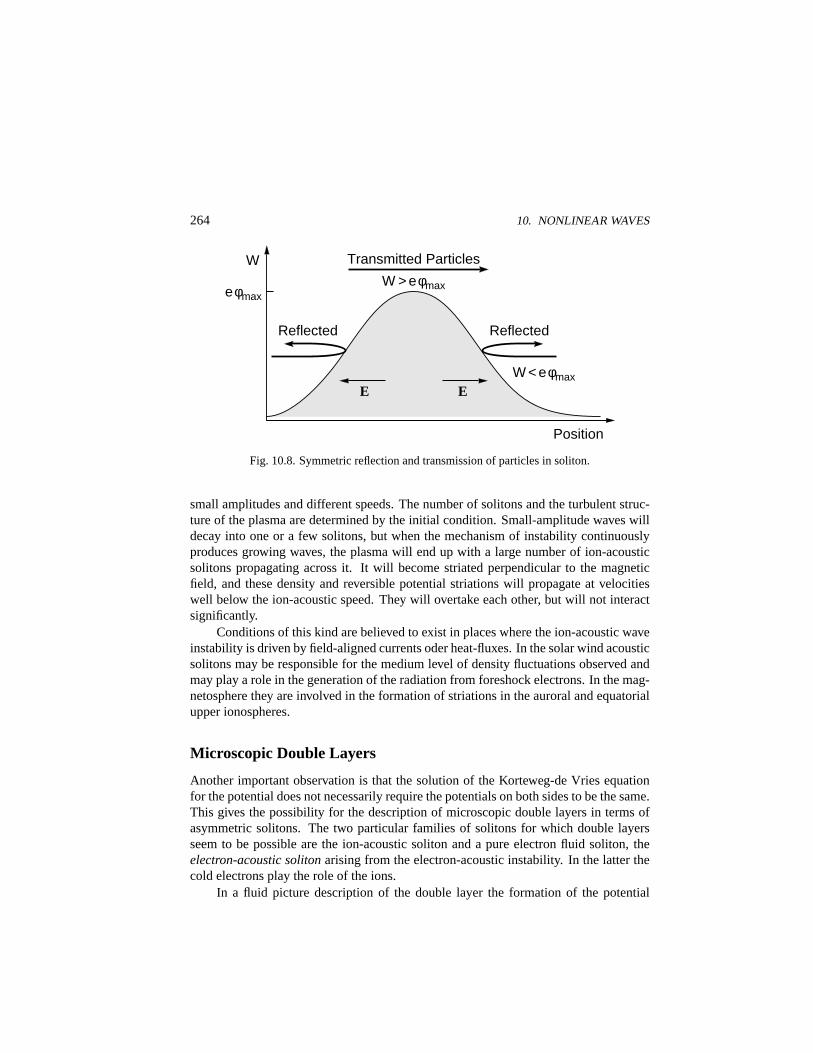
264 10. NONLINEAR WAVES
Transmitted Particles
Reflected Reflected
E E
eφmax
W < eφmax
W
W > eφmax
Position
Fig. 10.8. Symmetric reflection and transmission of particles in soliton.
small amplitudes and different speeds. The number of solitons and the turbulent struc-ture of the plasma are determined by the initial condition. Small-amplitude waves willdecay into one or a few solitons, but when the mechanism of instability continuouslyproduces growing waves, the plasma will end up with a large number of ion-acousticsolitons propagating across it. It will become striated perpendicular to the magneticfield, and these density and reversible potential striations will propagate at velocitieswell below the ion-acoustic speed. They will overtake each other, but will not interactsignificantly.
Conditions of this kind are believed to exist in places where the ion-acoustic waveinstability is driven by field-aligned currents oder heat-fluxes. In the solar wind acousticsolitons may be responsible for the medium level of density fluctuations observed andmay play a role in the generation of the radiation from foreshock electrons. In the mag-netosphere they are involved in the formation of striations in the auroral and equatorialupper ionospheres.
Microscopic Double Layers
Another important observation is that the solution of the Korteweg-de Vries equationfor the potential does not necessarily require the potentials on both sides to be the same.This gives the possibility for the description of microscopic double layers in terms ofasymmetric solitons. The two particular families of solitons for which double layersseem to be possible are the ion-acoustic soliton and a pure electron fluid soliton, theelectron-acoustic solitonarising from the electron-acoustic instability. In the latter thecold electrons play the role of the ions.
In a fluid picture description of the double layer the formation of the potential
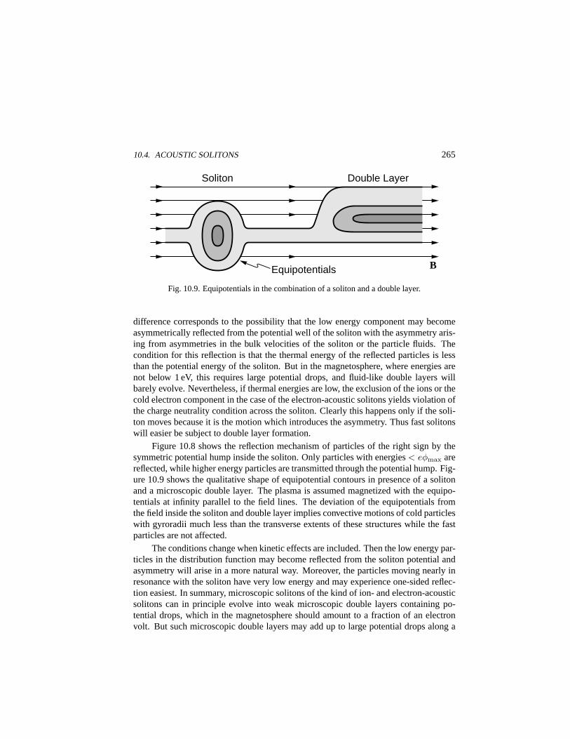
10.4. ACOUSTIC SOLITONS 265
Equipotentials
Soliton Double Layer
B
Fig. 10.9. Equipotentials in the combination of a soliton and a double layer.
difference corresponds to the possibility that the low energy component may becomeasymmetrically reflected from the potential well of the soliton with the asymmetry aris-ing from asymmetries in the bulk velocities of the soliton or the particle fluids. Thecondition for this reflection is that the thermal energy of the reflected particles is lessthan the potential energy of the soliton. But in the magnetosphere, where energies arenot below 1 eV, this requires large potential drops, and fluid-like double layers willbarely evolve. Nevertheless, if thermal energies are low, the exclusion of the ions or thecold electron component in the case of the electron-acoustic solitons yields violation ofthe charge neutrality condition across the soliton. Clearly this happens only if the soli-ton moves because it is the motion which introduces the asymmetry. Thus fast solitonswill easier be subject to double layer formation.
Figure 10.8 shows the reflection mechanism of particles of the right sign by thesymmetric potential hump inside the soliton. Only particles with energies< eφmax arereflected, while higher energy particles are transmitted through the potential hump. Fig-ure 10.9 shows the qualitative shape of equipotential contours in presence of a solitonand a microscopic double layer. The plasma is assumed magnetized with the equipo-tentials at infinity parallel to the field lines. The deviation of the equipotentials fromthe field inside the soliton and double layer implies convective motions of cold particleswith gyroradii much less than the transverse extents of these structures while the fastparticles are not affected.
The conditions change when kinetic effects are included. Then the low energy par-ticles in the distribution function may become reflected from the soliton potential andasymmetry will arise in a more natural way. Moreover, the particles moving nearly inresonance with the soliton have very low energy and may experience one-sided reflec-tion easiest. In summary, microscopic solitons of the kind of ion- and electron-acousticsolitons can in principle evolve into weak microscopic double layers containing po-tential drops, which in the magnetosphere should amount to a fraction of an electronvolt. But such microscopic double layers may add up to large potential drops along a
266 10. NONLINEAR WAVES
magnetic field line if they are aligned along the field with correct polarity.Let us consider electron-acoustic double layers. The basic one-dimensional fluid
equations for the cold,s = c, and warm,s = h, electron components and neutralizingcold ion,s = i, background are
∂ns
∂t+∇x(nsvs) = 0
msns
(∂vs
∂t+ vs∇xvs
)= −∇xps − ns∇xφ (10.78)
∂ps
∂t+ vs∇xps + ps∇xvs = 0
which must be completed by the Poisson equation
∇2xφ = n0h exp φ−
∑
s=i,c
ns (10.79)
The quantities have been normalized for simplicity here. For instance, the normaliza-tion of the potential iseφ/kBTh→φ and so on. In addition one implies the followingboundary conditions
φ → 0 ∇xφ → 0 ∇2xφ → 0
ns → n0s ps → p0s vs → 0
for x →∞ (10.80)
In order to derive the nonlinear equation describing the double layer formation we in-troduce the following stretching transformation
ξ = ε(x− ut)τ = ε3t
(10.81)
which differs from the one used before. We now expand all fluid quantities and thepotential in powers ofε and follow the procedure described in the previous section. Wethen obtain the following nonlinear equation for the first order expansion term of thepotential
∂φ1
∂τ+
a1
2∇ξφ
21 + a2∇ξφ
31 + a3∇3
ξφ1 = 0 (10.82)
This is themodified Korteweg-de Vries equation. It contains a third order nonlinearityand is valid as long as|a1/a3| = O(ε), and the coefficients are
a1 = − (n0c/n0h)2 + 3(n0c/n0h + 4Tc)2(n0c/n0h)(n0c/n0h + 3Tc)1/2
a2 = − (n0c/n0h)4 − 15(n0c/n0h)2 − 180Tc(n0c/n0h)− 432T 2c
12(n0c/n0h)3(n0c/n0h + 3Tc)1/2(10.83)
a3 = (n0c/n0h)2/2n0c(n0c/n0h + 3Tc)1/2
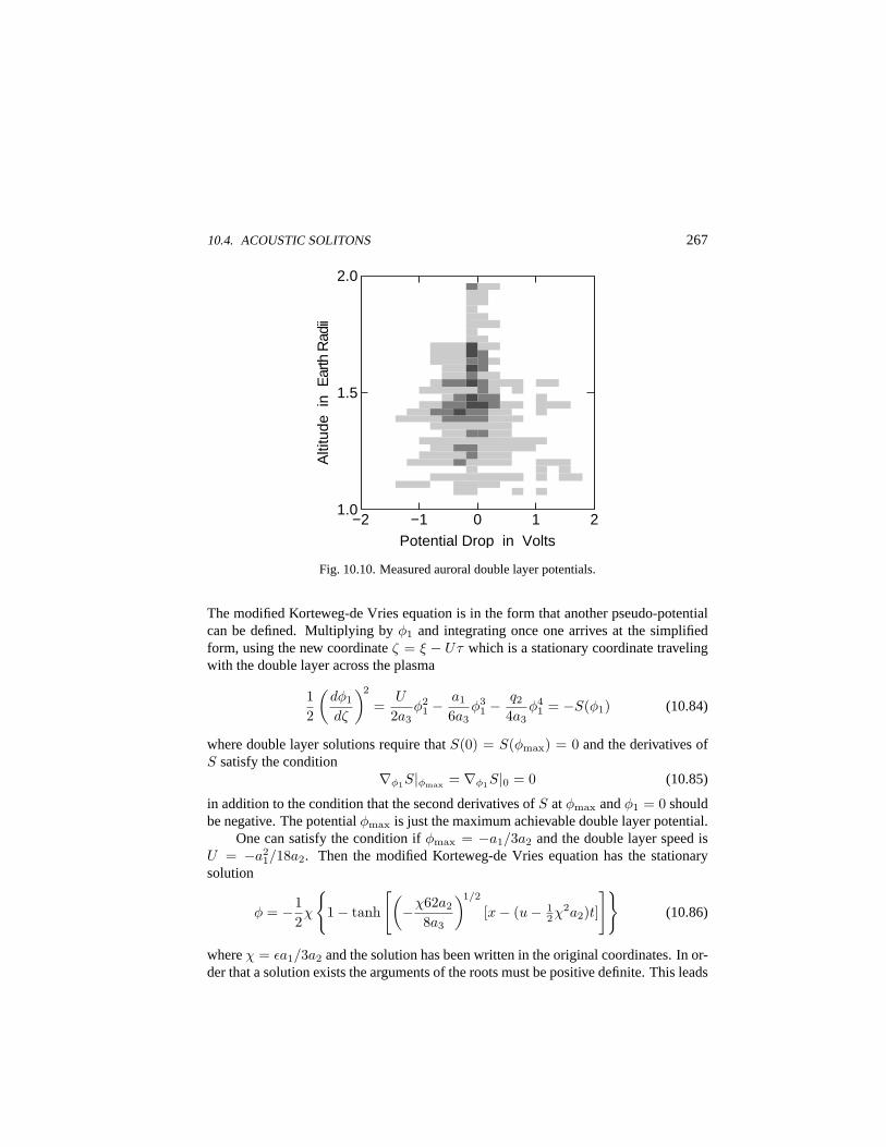
10.4. ACOUSTIC SOLITONS 267
−2 −1 1 2 1.0
1.5
2.0
Potential Drop in Volts
Alti
tude
in
Ear
th R
adii
0
Fig. 10.10. Measured auroral double layer potentials.
The modified Korteweg-de Vries equation is in the form that another pseudo-potentialcan be defined. Multiplying byφ1 and integrating once one arrives at the simplifiedform, using the new coordinateζ = ξ − Uτ which is a stationary coordinate travelingwith the double layer across the plasma
12
(dφ1
dζ
)2
=U
2a3φ2
1 −a1
6a3φ3
1 −q2
4a3φ4
1 = −S(φ1) (10.84)
where double layer solutions require thatS(0) = S(φmax) = 0 and the derivatives ofS satisfy the condition
∇φ1S|φmax = ∇φ1S|0 = 0 (10.85)
in addition to the condition that the second derivatives ofS atφmax andφ1 = 0 shouldbe negative. The potentialφmax is just the maximum achievable double layer potential.
One can satisfy the condition ifφmax = −a1/3a2 and the double layer speed isU = −a2
1/18a2. Then the modified Korteweg-de Vries equation has the stationarysolution
φ = −12χ
1− tanh
[(−χ62a2
8a3
)1/2
[x− (u− 12χ2a2)t]
](10.86)
whereχ = εa1/3a2 and the solution has been written in the original coordinates. In or-der that a solution exists the arguments of the roots must be positive definite. This leads
268 10. NONLINEAR WAVES
to a condition on the normalized cold plasma temperature as function of the densityratio
Tc = −45δ
216
1±
[1− 108
2025(15− δ2)
]1/2
(10.87)
whereδ = n0c/n0h is the density ratio which for solutions to exist needs to beδ >√15. Hence, as the theory demonstrates, electron-acoustic double layers are theoreti-
cally possible, but the restriction on their existence is rather severe requiring large coldelectron densities in which case any instability may become suppressed.
This is an interesting result which may throw some doubt onto the real existenceof stationary double layers in agreement with the experimental finding that only burstyand very low voltages have been observed in real plasmas. Figure 10.10 gives a feelingfor the realistic values of double layer potentials in the lower auroral magnetosphere asfunction of height above the Earth’s surface. Precise measurement of parallel electricpotentials is very difficult to perform. The voltages are differences between measuredand background potentials. Though occasionally potentials up to –2 V are detected, thedistribution of the voltages centers at very low potential values near zero. These dataindicate that most of the real double layers are very weak and microscopic double layerswhich may have arisen from particle reflection at solitary structures.
10.5. Alfven Solitons
Solitons exist also for low-frequency Alfven waves, both for the kinetic and shear ki-netic modes. We will not go through the whole process of reductive perturbation, butlook for solutions which are stationary in the frame of the traveling structure.
Kinetic Alfv en Solitons
As we know, there are two kinetic Alfven modes, one for plasma betaβ > me/mi,the other underβ < me/mi conditions. Remembering the two different dispersionrelations
ω =
k‖vA(1 + k2
⊥r2gi)
1/2 for β > me/mi
k‖vA(1 + k2⊥c2/ω2
pe)−1/2 for β < me/mi
(10.88)
we first find that kinetic Alfven solitons, if they exist, are intrinsically two-dimensional.The second observation is that solitons resulting from the first of these dispersion re-lation, which describes the proper kinetic mode, have dispersive properties differentfrom those of the ion-acoustic and electron-acoustic modes discussed so far. The shearkinetic mode described by the second of the dispersion relations, on the other hand, hasdispersive properties similar to the ion-acoustic wave. These differences will necessar-ily affect the properties of the solitons resulting from the underlying dynamics.

10.5. ALFVEN SOLITONS 269
Let us consider the kinetic mode first, because it promises to confront us withsome new effects. Referring to the fluid picture, we use the representation with twoelectric potentials (cf. Sec. 10.6 of our companion book,Basic Space Plasma Physics),E⊥ = −∇⊥φ⊥, E‖ = −∇‖φ‖. Assuming quasineutrality,ni = ne, and Boltzmann-distributed electrons
ne = n0 exp(eφ‖/kBTe) (10.89)
the basic equations describing the evolution of nonlinear kinetic Alfven waves are
∂B⊥∂t
= ∇⊥∇‖(φ⊥ − φ‖)
∇2⊥∇2
‖(φ⊥ − φ‖) = µ0∇‖∂j‖∂t
(10.90)
∂ni
∂t=
1ωgiB0
∇⊥(
ni∇⊥ ∂φ⊥∂t
)
The field-aligned current is entirely carried by the hot electron component. Hence
∇‖j‖ = e(∂ne/∂t) (10.91)
In dimensionless variables, withξ → xωgi/cia, ζ → zωpi/c, τ → ωgit, n → n/n0,eφ⊥/kBTe → φ⊥, eφ‖/kBTe → φ‖, this system of equations can be made stationarywhen transforming to the following co-moving coordinate
η = κ⊥ξ + κ‖ζ − τ (10.92)
This coordinate is introduced in order to transform to a frame which moves togetherwith the localized kinetic Alfvenic structure. However, in the present case it is impor-tant to note that this motion is neither parallel nor perpendicular to the magnetic field,but is a two-dimensional motion in a direction oblique to the external field. It turns outthat the system of fundamental equations allows for such a transformation, reducing thephysics to a one-dimensional problem.
Being interested in localized solutions, the boundary conditions at infinity are cho-sen such that the derivatives of the density parallel and perpendicular to the magneticfield vanish at infinity,∇⊥n = 0 at ξ→±∞, and∇‖n = 0 at ζ →±∞. Hence, ex-pressed in terms of the potentials, this implies that the potentials and their first, second,and third derivatives vanish at infinity. Under these conditions it is easy to see that thesystem of equations becomes stationary and does not explicitly depend on time. Onemay combine it and integrate it one to find the following equation
κ2⊥κ2
‖nd2 ln n
dη2= (1− n)(n− κ2
‖) (10.93)
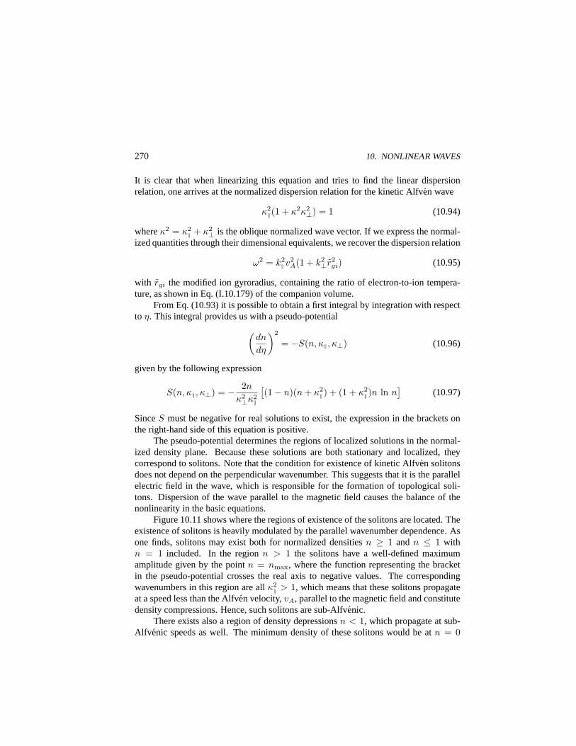
270 10. NONLINEAR WAVES
It is clear that when linearizing this equation and tries to find the linear dispersionrelation, one arrives at the normalized dispersion relation for the kinetic Alfven wave
κ2‖(1 + κ2κ2
⊥) = 1 (10.94)
whereκ2 = κ2‖ + κ2
⊥ is the oblique normalized wave vector. If we express the normal-ized quantities through their dimensional equivalents, we recover the dispersion relation
ω2 = k2‖v
2A(1 + k2
⊥r2gi) (10.95)
with rgi the modified ion gyroradius, containing the ratio of electron-to-ion tempera-ture, as shown in Eq. (I.10.179) of the companion volume.
From Eq. (10.93) it is possible to obtain a first integral by integration with respectto η. This integral provides us with a pseudo-potential
(dn
dη
)2
= −S(n, κ‖, κ⊥) (10.96)
given by the following expression
S(n, κ‖, κ⊥) = − 2n
κ2⊥κ2
‖
[(1− n)(n + κ2
‖) + (1 + κ2‖)n ln n
](10.97)
SinceS must be negative for real solutions to exist, the expression in the brackets onthe right-hand side of this equation is positive.
The pseudo-potential determines the regions of localized solutions in the normal-ized density plane. Because these solutions are both stationary and localized, theycorrespond to solitons. Note that the condition for existence of kinetic Alfven solitonsdoes not depend on the perpendicular wavenumber. This suggests that it is the parallelelectric field in the wave, which is responsible for the formation of topological soli-tons. Dispersion of the wave parallel to the magnetic field causes the balance of thenonlinearity in the basic equations.
Figure 10.11 shows where the regions of existence of the solitons are located. Theexistence of solitons is heavily modulated by the parallel wavenumber dependence. Asone finds, solitons may exist both for normalized densitiesn ≥ 1 andn ≤ 1 withn = 1 included. In the regionn > 1 the solitons have a well-defined maximumamplitude given by the pointn = nmax, where the function representing the bracketin the pseudo-potential crosses the real axis to negative values. The correspondingwavenumbers in this region are allκ2
‖ > 1, which means that these solitons propagateat a speed less than the Alfven velocity,vA, parallel to the magnetic field and constitutedensity compressions. Hence, such solitons are sub-Alfvenic.
There exists also a region of density depressionsn < 1, which propagate at sub-Alfv enic speeds as well. The minimum density of these solitons would be atn = 0
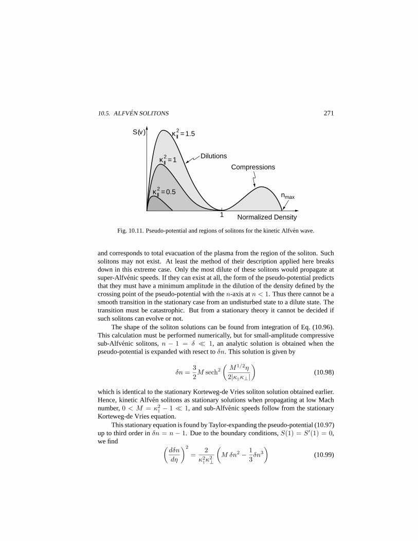
10.5. ALFVEN SOLITONS 271
Dilutions
Compressions
nmax
κ2|| = 1.5
κ2|| = 1
κ2|| = 0.5
Normalized Density
S(v )
1
Fig. 10.11. Pseudo-potential and regions of solitons for the kinetic Alfven wave.
and corresponds to total evacuation of the plasma from the region of the soliton. Suchsolitons may not exist. At least the method of their description applied here breaksdown in this extreme case. Only the most dilute of these solitons would propagate atsuper-Alfvenic speeds. If they can exist at all, the form of the pseudo-potential predictsthat they must have a minimum amplitude in the dilution of the density defined by thecrossing point of the pseudo-potential with then-axis atn < 1. Thus there cannot be asmooth transition in the stationary case from an undisturbed state to a dilute state. Thetransition must be catastrophic. But from a stationary theory it cannot be decided ifsuch solitons can evolve or not.
The shape of the soliton solutions can be found from integration of Eq. (10.96).This calculation must be performed numerically, but for small-amplitude compressivesub-Alfvenic solitons,n − 1 = δ ¿ 1, an analytic solution is obtained when thepseudo-potential is expanded with resect toδn. This solution is given by
δn =32M sech2
(M1/2η
2|κ‖κ⊥|)
(10.98)
which is identical to the stationary Korteweg-de Vries soliton solution obtained earlier.Hence, kinetic Alfven solitons as stationary solutions when propagating at low Machnumber,0 < M = κ2
‖ − 1 ¿ 1, and sub-Alfvenic speeds follow from the stationaryKorteweg-de Vries equation.
This stationary equation is found by Taylor-expanding the pseudo-potential (10.97)up to third order inδn = n − 1. Due to the boundary conditions,S(1) = S′(1) = 0,we find (
dδn
dη
)2
=2
κ2‖κ
2⊥
(M δn2 − 1
3δn3
)(10.99)
272 10. NONLINEAR WAVES
If we now take the second derivative of both sides of this equation, we arrive at thedesired equation
δn′ +2M
δn δn′ − δn′ − κ2‖κ
2⊥
Mδn′′′ = 0 (10.100)
Supplementing it by the missing time derivative, a form of the Korteweg-de Vries equa-tion is recovered. As we expected, low but finite amplitude sub-Alfvenic compressivekinetic Alfven waves evolve into solitons under the competitive action of their nonlin-earity and their dispersive properties. If an initial condition is given, one thus expectsthat kinetic Alfven waves decay into a chain of low amplitude solitons which may bedistributed according to their amplitudes by a distribution law of the kind given in Eq.(10.55).
Because there is no threshold for this kind of evolution of kinetic Alfven waves,they will always tend to evolve into solitons. Soliton formation will be restricted onlyby other factors as the dimensions of the system, inhomogeneities, wave transformationand wave coupling. The number of solitons which can be formed depends not onlyon the initial disturbance but also on the available length of the field lines. In themagnetosphere this length is restricted by two conditions, the value of the plasma betaand the distance between the point whereβ > me/mi and the plasma sheet. Alongthis length a magnetic pulse injected from the plasma sheet by, say, reconnection canbreak off into a number of kinetic Alfven solitons, which travel as low amplitude pulsesinto the inner magnetosphere up to the point whereβ < me/mi, where they possiblytransform into shear kinetic Alfven waves. The larger amplitude solitons will propagateat higher speed and may overcome the lower amplitude pulses. How the transformationworks is unknown. The simplest way is that at the altitude of transition fromβ >me/mi to β < me/mi the incoming kinetic Alfven solitons serve as initial conditionsfor the evolution of shear kinetic Alfven solitons.
Shear Kinetic Alfv en Solitons
Shear kinetic Alfven waves can evolve into solitons in a way entirely analog to kineticAlfv en waves. The difference in the dispersive properties of the two modes suggeststhat shear kinetic waves behave similar to ion-acoustic solitons with a negative disper-sion factor.
It is simple matter to derive the pseudo-potential for these waves and to discussthe conditions of existence of such solitons. The dynamics of low-amplitude solitons isalso governed by a Korteweg-de Vries equation, but the solitons have slightly differentproperties. The basic equations for this case are the same as for the former case, withthe exception that one replaces the Boltzmann law for the electrons with the full com-pressive electrons dynamics, as before in dimensionless variables
10.5. ALFVEN SOLITONS 273
∂ne
∂τ+∇ζ(neve) = 0
∂ve
∂τ+ 1
2∇ζv2e = 1
2α∇ζ [φ‖ − ln ne](10.101)
The coefficientα is defined asα = (mi/me)βe, whereβe is the electron plasma beta.We change to the co-moving coordinates,η = κ‖ζ + κ⊥ξ − τ , and use homogeneousboundary conditions at infinity. The basic equations then reduce to
(n− κ‖nve)′ = 0(ve − 1
2κ‖v2e
)′= − 1
2ακ‖(φ‖ − ln n)′(n− κ2
⊥nφ′′⊥)′
= 0
κ2⊥κ‖(φ⊥ − φ‖)′′′′ = (nve)′′
(10.102)
The primes indicate the number of total derivatives with respect to the co-moving coor-dinateη.
The last equation can be integrated twice, the other equations once inη from−∞to η, and the variables may be expressed by the quasineutral normalized density,n
ve = (n− 1)/nκ‖
φ‖ = lnn + [(1− n2)/ακ2‖n
2]φ′′⊥ = (κ‖/κ⊥)ve
φ′′‖ = −(1− n)(n− κ2‖)/nκ2
⊥κ2‖
(10.103)
Sinceφ‖ depends only implicitly onη and since all variables can be expressed throughthe density,n(η), it is sufficient to consider only the last of the above equations and tosolve forφ‖. This equation is readily transformed into a form containing the pseudo-potential. We chose to write it as
12
(dn
dη
)2
=S(n; α, κ‖)
κ2⊥F 2(n; α, κ‖)
(10.104)
where we haveF = (ακ2‖/2)Ψ(n) andΨ(n) = (1− 2/n2ακ2
‖)/n. Then we can write
S = [Ψ2(n)κ2⊥κ2
‖]−1
∫ n
1
1− ξ
ξ(ξ − κ2
‖)Ψ(ξ) dξ (10.105)
Solving the last integral, the pseudo-potential becomes explicitly
S =α2κ2
‖
4
[1− n
n(n + κ2
‖) + (1 + κ2‖) ln n +
(1− n)2
αn2
(1κ2‖− n + 2
3n
)](10.106)
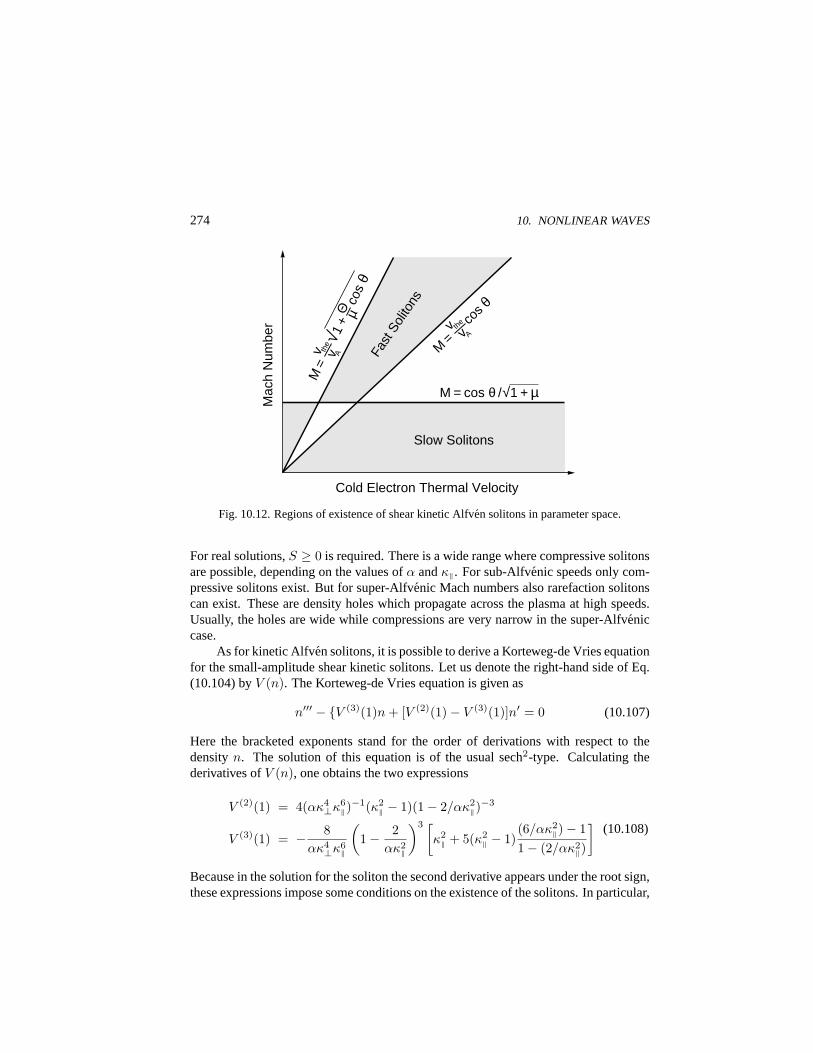
274 10. NONLINEAR WAVES
Fast
Sol
itons
Slow Solitons
Cold Electron Thermal Velocity
Mac
h N
umbe
r
M = cos θ /√1 + µ
M=v the
cos θ
vA v A
µ
M=
v the √1
+Θ
cos
θ
Fig. 10.12. Regions of existence of shear kinetic Alfven solitons in parameter space.
For real solutions,S ≥ 0 is required. There is a wide range where compressive solitonsare possible, depending on the values ofα andκ‖. For sub-Alfvenic speeds only com-pressive solitons exist. But for super-Alfvenic Mach numbers also rarefaction solitonscan exist. These are density holes which propagate across the plasma at high speeds.Usually, the holes are wide while compressions are very narrow in the super-Alfveniccase.
As for kinetic Alfven solitons, it is possible to derive a Korteweg-de Vries equationfor the small-amplitude shear kinetic solitons. Let us denote the right-hand side of Eq.(10.104) byV (n). The Korteweg-de Vries equation is given as
n′′′ − V (3)(1)n + [V (2)(1)− V (3)(1)]n′ = 0 (10.107)
Here the bracketed exponents stand for the order of derivations with respect to thedensityn. The solution of this equation is of the usual sech2-type. Calculating thederivatives ofV (n), one obtains the two expressions
V (2)(1) = 4(ακ4⊥κ6
‖)−1(κ2
‖ − 1)(1− 2/ακ2‖)−3
V (3)(1) = − 8ακ4
⊥κ6‖
(1− 2
ακ2‖
)3 [κ2‖ + 5(κ2
‖ − 1)(6/ακ2
‖)− 11− (2/ακ2
‖)
](10.108)
Because in the solution for the soliton the second derivative appears under the root sign,these expressions impose some conditions on the existence of the solitons. In particular,

10.5. ALFVEN SOLITONS 275
Den
sity
0 −1 1
3
Distance η
Cold Dilution
Hot Compression
2
1
Fig. 10.13. Cold plasma depletion containing a hot electron sheet.
for compressive kinetic Alfven solitons to exist one can derive the restriction
2(vA/vthc)2 < κ2‖ < 7(vA/vthc)2 (10.109)
which must be satisfied simultaneously withκ2‖ < 1.5. Combining both we find the
condition on the Mach number for shear kinetic compressive solitons (θ is the anglebetween the original wave and the ambient magnetic field)
17 (vA/vthc) cos2 θ < M2 < 1
2 (vA/vthc) cos2 θ (10.110)
The corresponding condition for sub-Alfvenic rarefactive solitons to exist is
M2 < 17 (vA/vthc) cos2 θ (10.111)
Two-Electron Kinetic Alfv en Solitons
We now investigate one particularly interesting case when the plasma contains twoelectron components of different densities and temperatures. The cold and hot electronpopulations are indexed by the subscriptsc andh, respectively. Quasineutrality requiresthat, in normalized coordinates,
ni = (nc + µnh)/(1 + µ) (10.112)
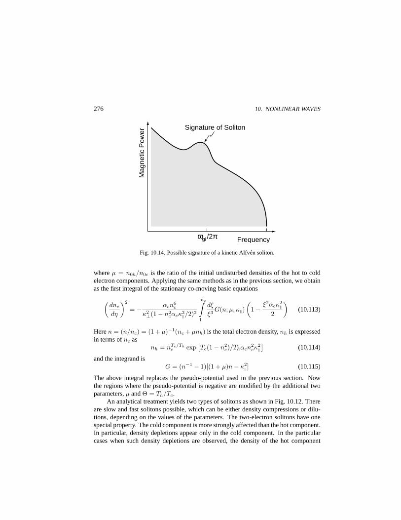
276 10. NONLINEAR WAVES
ωgi /2π Frequency
Mag
netic
Pow
er Signature of Soliton
Fig. 10.14. Possible signature of a kinetic Alfven soliton.
whereµ = n0h/n0c is the ratio of the initial undisturbed densities of the hot to coldelectron components. Applying the same methods as in the previous section, we obtainas the first integral of the stationary co-moving basic equations
(dnc
dη
)2
= − αcn6c
κ2⊥(1− n2
cαcκ2‖/2)2
nc∫
1
dξ
ξ3G(n; µ, κ‖)
(1− ξ2αcκ
2‖
2
)(10.113)
Heren = (n/nc) = (1 + µ)−1(nc + µnh) is the total electron density,nh is expressedin terms ofnc as
nh = nTc/Thc exp
[Tc(1− n2
c)/Thαcn2cκ
2‖]
(10.114)
and the integrand isG = (n−1 − 1)[(1 + µ)n− κ2
‖] (10.115)
The above integral replaces the pseudo-potential used in the previous section. Nowthe regions where the pseudo-potential is negative are modified by the additional twoparameters,µ andΘ = Th/Tc.
An analytical treatment yields two types of solitons as shown in Fig. 10.12. Thereare slow and fast solitons possible, which can be either density compressions or dilu-tions, depending on the values of the parameters. The two-electron solitons have onespecial property. The cold component is more strongly affected than the hot component.In particular, density depletions appear only in the cold component. In the particularcases when such density depletions are observed, the density of the hot component
10.6. DRIFT WAVE TURBULENCE 277
peaks in the center of the cold depletion, forming a compressive hot electron structureinside the diluted cold plasma. Figure 10.13 shows one example of such a soliton. Thecold plasma depletion contain a hot electron layer, with the peak density of the hotelectrons raised by more than a factor ten in order to compensate for the cold electrondecrease. It is the concentration of the hot electrons which pushes the cold plasma outof the center of the soliton.
Two-electron plasmas are frequently encountered in space plasma physics. In theplasmasphere it is the mixture of the ring current plasma and the low energy plasma-spheric plasma of atmospheric origin. At auroral latitudes the mixture of cold iono-spheric and warm plasma sheet plasma leads to conditions where the present theory ofkinetic Alfven solitons is applicable. In the region of the low-latitude boundary layeradjacent to the magnetopause the warm magnetospheric plasma blends into the coldmagnetosheath plasma on a scale where kinetic Alfven waves and solitons may formand contribute to the dynamics. An example of the presumable observation of the sig-nature of a kinetic Alfven soliton in the low latitude boundary layer with frequencyclose to the ion-cyclotron frequency is given in Fig. 10.14.
10.6. Drift Wave Turbulence
Weak drift wave turbulence is described by the Hasegawa-Mima equation (9.40) in thetwo-dimensional approximation, which is based on wave-wave interactions. When thedrift waves evolve nonlinearly, the weakly turbulent wave-wave interaction approxima-tion breaks down. The drift waves may decay into large-amplitude solitons. When suchsolitons appear in large numbers, they constitute a state of turbulence which is verydifferent from weak turbulence and deserves the name ofstrong turbulence.
Drift Wave Solitons
We consider the simplest case of drift waves when the electrons, for low wave frequen-cies, can be considered as Boltzmann-distributed, and the ions as cold. Then the ionsperform a simpleE×B-drift in the crossed ambient magnetic and wave electric fields,a process which provides the nonlinearity, because when the waves are driven by theions, as in the case of the lower-hybrid drift instability, this coupling couples the waveback to the motion of the ions. The waves, with their perpendicular and parallel electricfield components, propagate obliquely to the magnetic field. We introduce the densityand temperature scalesLn andLT and scale all lengths with respect torgi = cia/ωgi.
Because of the obliqueness of the problem the nonlinear wave is two-dimensional.It is governed by theKadomtsev-Petviashvili equation, which is the two-dimensionalgeneralization of the Korteweg-de Vries equation. But fork2
⊥r2gi < 1 andkyk2
⊥r3gi ¿
278 10. NONLINEAR WAVES
rgi/LT this equation can be reduced to the Korteweg-de Vries equation proper
∂φ
∂τ+∇⊥φ +∇3
⊥φ− φ∇⊥φ = 0 (10.116)
for the normalized electrostatic potential,φ(x, t). Here timeτ is measured in units ofrgi/vde, where the drift velocity isvde = rgicia/Ln = kBTe/eB0Ln.
In the linear approximation the system evolves into drift modes which are eigen-modes of the system considered. Because the nonlinear evolution of these drift wavesis governed by the Korteweg-de Vries equations, we expect that solitons will be gener-ated in large number for sufficiently large initial wave amplitudes, and the system willbecome turbulent consisting of non-interacting solitons of frequency,ω(k) ≈ kvde, anddispersion relationωs = ku, whereu > vde is the soliton speed. The drift wave field isthen assumed to be composed of a large numberN of solitons
φ(x, τ) =N∑
l=1
φs(x, τ, xl, ul) (10.117)
each having a different central position,xl, and speed,ul, with the speed satisfying thesoliton dispersion relation. Since the single solitons are nearly independent solutions ofthe Korteweg-de Vries equation, their analytical representation is of the form
φs(x, τ, x0, u) = −3(u− 1)sech2[ 12 (u− 1)1/2(x− x0 − uτ)] (10.118)
Collisions are elastic and produce only an unimportant phase shift of the soliton posi-tion.
The inverse scattering method gives us the possibility to define a distribution func-tion of the soliton amplitudes and velocities, given in Eq. (10.55). The soliton amplitudeis A = 3(u− 1). With β = ` = 1 and3u0→A, we haveσ = 1/3 and
F [u] =1
12π
∫
φ<−A/2
dx
[−2φ(x)−A]1/2(10.119)
a formula which is valid for the negative-potential drift wave solitons withφ < 0.
Spectrum of Drift Wave Solitons
Equation (10.119) may serve as starting point for a statistical description through anaverage over initial configurations. One may assume that the final turbulent state isreached as the most probable state of a number of initial configurations, such thatthe system containing many solitons will saturate at some randomly phased spectrum,〈|φ(k)|2〉, with the angular brackets indicating the averaging procedure, andφ(k) being
10.6. DRIFT WAVE TURBULENCE 279
the Fourier transformed potential amplitude. The spread of the random-phased field,φ,can be taken as given by some mean square amplitude,〈|φ|2〉 = φ2
0.Given such an initial amplitude, knowing the distribution (10.119) of soliton am-
plitudes resulting from the solution of the Korteweg-de Vries equation, the distributionof solitons can be obtained by calculating the average overF [u] with random-phasedamplitudes. For a broad wavenumber spectrum the initial spectrum can be taken aswhite noise. Then the average ofF [u] is a Gaussian integral written in discrete form as
fsol(u) =1Z
l∏
j=1
∫dφj exp
[−φ2
j
2φ20
]F [u; φ] (10.120)
Normalization requires that the integral overu-space just gives the total number ofsolitons in the system ∫ ∞
vde
fsol(u)du = N (10.121)
Moreover, the indexed potentials are the soliton potential functions at positionsxj . Itis now possible to convert the integral in the functionalF [u] into a sum and to performthe Gaussian integrations. Using a representation of the parabolic cylinder functionD−1/2(x) one finds
fsol(u) =1
24π
L√φ0
exp[−9(u− 1)2
16φ20
]D−1/2
[3(u− 1)
2φ0
](10.122)
L is the length of the system, defined asL =∑l
j xj , wherexj = (j/l)L. This is thedistribution function for drift wave solitons, which is provided in drift wave turbulencearising from the random-phased initial condition with amplitudeφ0. The distributionof the soliton velocities turns out to be not purely Gaussian even in this simple caseof strong turbulence. The parabolic cylinder function introduces a skewing into thedistribution which is caused by the concentration of the wave energy in the solitarywave solutions of the Korteweg-de Vries equation. As one of the consequences theturbulent spectrum gets harder than a spectrum of randomly distributed waves.
It is not very difficult to calculate the spectral density of the soliton field know-ing the distribution function. The spectral density,S(k, ω), is defined as the Fouriertransform of the two-point correlation function. Takingφsol from Eq. (10.117) and cal-culating the Fourier transform of〈φsol(x+ ζ, t+ τ)φsol(x, t)〉 one finds for the spectralshape
S(k, ω) =96k2
√3L
fsol
(ω
k
)cosech2
[πkrgi
(kvde
ω − kvde
)1/2]
(10.123)
280 10. NONLINEAR WAVES
Note thatk, vde, L are all normalized quantities. This result has been obtained by re-placing the sum over the solitons inφsol with an integral using the soliton distribution,fsol, as weight, andu = ω/k, which is justified for a large number of solitons. Thisnumber is defined as
N =∫ ∞
vde
du fsol(u) = QLφ1/20 (10.124)
whereQ ≈ Γ(3/4)/119. The first important property of the spectrum of solitons isthat it vanishes for frequenciesω < kvde, simply because there are no solitons in thisrange with speeds smaller thanu < vde. Secondly, the spectrum peaks at frequenciesω ≈ kvde[1 + O(φ0)] above the lower frequency cut-off. If one expands the paraboliccylinder function for small and for large arguments these peaks are found at
ωmax ≈
kvde(1 +√
2φ0) for π2k2 ¿ φ0
kvde[1 +√
2(πkφ20)
2/5] for π2k2 À φ0
(10.125)
The interesting conclusion is thus that the calculation of the soliton spectrum verifiesthe suspicion that the turbulent spectrum of a soliton gas, in this case the drift-solitongas, is harder than the spectrum of drift waves themselves from which it developed.
Application of this kind of turbulence to waves in equatorial spread-F and to in-stabilities of the kind of the lower-hybrid drift instability in the Earth’s plasma sheetand low-latitude boundary layer seems promising, but has not yet been tried. Spectra inthese regions look relatively structureless and thus do point on the existence of evolvedscale-independent or self-similar turbulence.
Similar considerations may also apply to kinetic Alfven soliton turbulence, to ionacoustic turbulence and electron acoustic turbulence. For these waves it is known thatthe turbulence follows the Korteweg-de Vries equation as long as the amplitudes do notbecome too large. One may expect that when this happens, particle reflection at themany solitary structures in the turbulent plasma will produce dissipation and introduceirreversibility, and the second-order derivative will become non-negligible, small po-tential differences will arise, and the plasma will make the transition to micro-doublelayer turbulence. The existence of this kind of turbulence manifests itself in localizedholes in phase space and may be very important in particle acceleration.
Concluding Remarks
A number of equations has been derived in this chapter, which lead to localized large-amplitude wave solutions travelling across the plasma. The important insight is thatthese solitons evolve as nonlinear dynamical equilibria between nonlinearity and dis-persivity of single waves, but that the equations allow a given initial condition to decayinto a large number of such solitons, travelling at their own and well-defined speeds
10.6. DRIFT WAVE TURBULENCE 281
with negligible interaction, thus comprising a turbulent state of the plasma which canbe described in a statistical way.
A few examples are given in this chapter, e.g., ion-acoustic, electron-acoustic, ki-netic Alfven, and drift wave solitons. Their application to space plasmas is still open.The reason is that in spite of the well-known importance of soliton turbulence only fewobservations allow for an unambiguous interpretation in terms of solitons. In this situ-ation the link between theory and observation in space plasma physics is still missing.
Further Reading
There is a small number of excellent books on nonlinear plasma theory like [1], [5], and[11], which all were written in the seventies. Meanwhile nonlinear plasma physics hasgrown into a wide field, but no comprehensive modern text is available. The reason isthat analytically not so much has been achieved during the last twenty years while theactivities and interests have turned to numerical simulations. A contemporary summaryof numerical plasma simulations is given in [7].
Derivation of the Burgers and Korteweg-de Vries equations from the general hy-drodynamics set of Navier-Stokes equations is given in [4]. Derivation from plasmafluid equations are contained in [8]. The inverse scattering method has found wideapplication in the theory of one-dimensional nonlinear wave equations. It is given in[4], [8], and many other texts. Drift wave turbulence is treated in [3]. The doublelayer theory is taken from Mace and Hellberg,J. Plasma Phys. 49 (1993) 283. For theKadomtsev-Petviashvili equation we followed Meiss and Horton,Phys. Rev. Lett. 48(1982) 1362. Kinetic Alfven soliton theory is included in [2]. Double layer potentialswere measured by Malkki et al.,J. Geophys. Res. 99 (1994) 6045. Shear kinetic Alfvensoliton theory for one- and two-electron fluids is taken from Treumann et al.,Astron.Astrophys.236 (1990) 242. Observational information on shocks is found in [6] and[10]. Laminar and turbulent shocks are discussed in [9].
[1] R. C. Davidson,Methods in Nonlinear Plasma Theory(Academic Press, NewYork, 1972).
[2] A. Hasegawa and C. Uberoi,The Alfven Wave(U.S. Dept. of Energy, Springfield,1982).
[3] B. B. Kadomtsev,Plasma Turbulence(Academic Press, New York, 1965).
[4] V. I. Karpman,Nichtlineare Wellen in dispersiven Medien(Vieweg Verlag, Braun-schweig, 1977).
[5] R. Z. Sagdeev and A. A. Galeev,Nonlinear Plasma Theory(W. A. Benjamin, NewYork, 1969).
282 10. NONLINEAR WAVES
[6] R. G. Stone and B. T. Tsurutani (eds.),Collisionless Shocks in the Heliosphere: ATutorial Review(American Geophysical Union, Washington, 1985).
[7] T. Tajima,Computational Plasma Physics(Addison-Wesley Publ. Co., RedwoodCity, 1989).
[8] T. Taniuti and K. Nishihara,Nonlinear Waves(Pitman Advanced Publ., Boston,1983).
[9] D. A. Tidman and N. A. Krall,Shock Waves in Collisionless Plasmas(Wiley In-terscience, New York, 1971).
[10] B. T. Tsurutani and R. G. Stone (eds.),Collisionless Shocks in the Heliosphere:Reviews of Current Research(American Geophysical Union, Washington, 1985).
[11] V. N. Tsytovich,Nonlinear Effects in Plasmas(Plenum Press, New York, 1970).
11. Strong Turbulence
The previous chapter attempted the first step into strong turbulence theory. We consid-ered the evolution of large-amplitude waves when the dispersion competes with nonlin-earity and obtained that plasmas may in this case evolve into turbulent states containinglarge numbers of quasi-stable solitary waves, so-called topological solitons, which con-stitute turbulence.
Another important effect arising in a plasma is a consequence of the fact thatplasma waves are carriers of energy. The energy density stored in a plasma wave cor-responds to a real pressure exerted on the plasma. Any inhomogeneity developing onthe wave spectrum by localized reflection, for instance, by absorption or interactionwith other waves and particles or simply by focussing or spreading of a wave, causes awave-pressure force, theponderomotive force. This force appears as an ordinary forceon the particles or fluid and may act on the plasma and change the propagation proper-ties of the wave itself or may affect the propagation of other waves. It also may lead tointerchanges between the waves. We expect that under such conditions another type ofturbulence will develop and call itstrong turbulence, a term whose meaning will haveto be clarified in this chapter.
Strong turbulence has a number of different aspects. In a first step we are go-ing to derive the ponderomotive force which is exerted by the plasma wave pressureonto the background plasma. This can be done with the elementary knowledge of ba-sic plasma physics using a simple high-frequency wave model. The simple theory canthen be extended to a much more general case, but for the purposes of understandingthe elementary theory is sufficient. Hereafter, we consider the basic equations whichin the presence of nonlinearity and wave pressure govern strong turbulence. Solutionof these equations leads to caviton formation instead of solitons. Cavitons behave dif-ferently from solitons. Their dynamics will be discussed in detail for Langmuir wavesuncovering some entirely new effects.
283
284 11. STRONG TURBULENCE
11.1. Ponderomotive Force
The wave pressure force exerted by a large-amplitude wave on the plasma backgroundis the ponderomotive force of the inhomogeneous wave field experienced by the parti-cle components. Such forces can be generated by any wave transporting energy, i.e.,moving at a certain group velocity and thus being spatially inhomogeneous.
Radiation Pressure Force
The simplest example of such a force is the radiation pressure of a high-frequencyelectromagnetic field experienced by an isotropic medium of dielectric function givenin Eq. (I.9.36) of our companion book
ε(ω) = 1− ω2pe/ω2 (11.1)
The pressure force in this most simple case can be estimated as follows. The electricfield energy density is known to be given by
Ww =∂(ωε)∂ω
WE (11.2)
with WE = (ε0/2)|δE|2. This energy density is equal to the wave field pressure which,from the point of view of the background medium carrying the wave, behaves exactlylike an ordinary gas pressure acting on a hydrodynamic fluid. The radiation pressure orponderomotive forceis then simply defined as
Fpm = − 12n0
∇Ww (11.3)
where we divide by the number density in order to obtain the force acting on one par-ticle. There is an additional factor of 1/2 in this expression, the origin of which willbecome clear below. Inserting the expression for the dielectric function (11.1) and car-rying out the differentiations with respect to the frequency,ω, yields
Fpm =ε− 12n0
∇WE(x, t) +WE(x, t)
2n0∇ε (11.4)
For approximately constantε the last term disappears, and the ponderomotive pressureforce assumes the particularly simple form
Fpm =ε− 12n0
∇WE(x, t) = − ε0ω2pe
4n0ω2∇|δE(x, t|2 (11.5)
11.1. PONDEROMOTIVE FORCE 285
In the present case this force is a potential force, with potential given by
φpm = −ε(ω)− 12n0
WE =e2
4meω2|δE|2 (11.6)
Because the Debye length is much smaller than the characteristic length of the fieldinhomogeneity, the electrons obey the Boltzmann law in the ponderomotive force po-tential
ne = n0 exp[−φpm/kB(Te + Ti)] = n0 exp[−|δE(x, t)|2/E2c ] (11.7)
where the ponderomotive critical electric field is given by
E2c = 4meω
2kB(Te + Ti)/e2 (11.8)
Therefore, for wave electric field intensities coming close to the critical electric field,the nonlinear pressure force effects become large and the distortions of the plasmadensity may become of the same order as the background density.
Density Variation
The nonlinear ponderomotive effect may result in a violent modification of the plasmabackground caused by the waves, in which case the plasma looses its homogeneouscharacter, but changes on a comparably short spatial scale. This is a typical propertyof turbulence. Strong turbulence may thus be caused by the ponderomotive effects oflarge amplitude waves. The nonlinear distortion of the density for moderate turbulenceis obtained from the Boltzmann law by small amplitude expansion
δnnl/n0 ≈ −|δE(x, t)|2/E2c (11.9)
This variation in the density is a negative modulation. For the model under considera-tion the expected modulation of the background plasma density in presence of a large-amplitude electromagnetic wave, which exerts a radiation pressure onto the plasma, theexpected density variation will always result in a local decrease of the plasma densityin the region of large amplitudes. Such depletions of density are usually calledcavitonsand should be distinguished from the ordinary or topological solitons discussed in theprevious chapter, because of the entirely different physics involved in their productionand evolution.
It should, however, be mentioned that the consideration of the ponderomotive forcein this section is not restricted to the radiation pressure of the electromagnetic wave.Our only assumption was that the wave frequency should be high enough to neglectother effects. Therefore the same argument also applies to Langmuir waves. Theirresponse function is the same, since their high frequencies radiation pressure works inexactly the same way as discussed above. But because Langmuir waves have very lowphase and group velocities, their ponderomotive effect may even be stronger than thatof electromagnetic waves when their energy accumulates locally.
286 11. STRONG TURBULENCE
Fluid Theory
The intuitive approach to the ponderomotive force given in the previous section mustbe based on safer grounds and at the same time must be extended to arbitrary large-amplitude waves. It is easiest to start from the hydrodynamic set of equations of aplasma and to average over the fast time scale of the large-amplitude wave. Dependingon the fluid model used one obtains different results.
Here we only sketch the derivation of the ponderomotive force. The simplestmodel is that of a magnetohydrodynamic fluid. We assume that the fluid is subjectto a nonlinear large-amplitude magnetohydrodynamic or electromagnetic wave
[δB(x, t), δE(x, t)] = [δB0(x, t), δE0(x, t)] exp(k · x− ωt) (11.10)
where the amplitudes are slowly varying functions of space and time. The nonlinearterms in the magnetohydrodynamic equations, i.e., the convective derivative,v · ∇v,the flux term,nv, and the Lorentz force term,j×B, contain products of the amplitudesand after fast-time and fast-space averaging will contribute to a wave force term.
The easiest way is to calculate the components of the wave stress tensor,Σ, undersuch an averaging. The ponderomotive force density is then defined as
fpm(x, t) = ∇ ·Σ (11.11)
When the wave amplitude depends on space and time as a slowly varying function,i.e., when the wave field is inhomogeneous and varying, the ponderomotive force willalso be a function of space and time. Performing the calculations, one finds that theponderomotive force density obtained is composed of two terms according to
fpm(x, t) = fpm,∇(x, t) + fpm,t(x, t) (11.12)
The first term results from the spatial dependence of the wave amplitude and is givenby
fpm,∇ =ε04
[∇
(δE∗
l δEm n∂εlm
∂n
)− δE∗
l δEm
(∇εlm − ∂εlm
∂B0j∇B0j
)](11.13)
Here we have written the tensorε = εlm in index notation. It depends on the plasmadensity,n, and on the ambient magnetic field,B0.
The second term in (11.12) comes from the slow time variation of the wave ampli-tude and is given by
fpm,t =ε0
4µ0
∂
∂t[(ε− I) · δE× δB∗] +
[(ω
∂ε
∂ω· ∂δE
∂t
)× δB∗
]+ c.c.
(11.14)
where c.c. stands for the conjugate complex part. These expressions simplify for planecircularly polarized waves of parallel wavenumber,k‖, and frequency,ω. In this case
11.2. NONLINEAR WAVE EQUATION 287
one simply adds the two components of the ponderomotive force
fpm‖ =ε− 1
2∇‖WE +
k‖2ω2
∂ω2(ε− 1)∂ω
∂WE
∂t
fpm⊥ = −12
∂ω(ε− 1)∂ω
∇⊥WE − B0
µ0∇⊥δB‖
(11.15)
to the stationary Lorentz force on the right-hand side of the equation of motion. Forvanishing time dependence and otherwise homogeneous conditions and for an inci-dent electromagnetic wave one recovers the simple wave pressure force of the previoussection. But already Alfven or whistler waves in the stationary case give different ex-pressions for the ponderomotive force than the simple pressure force.
When the magnetohydrodynamic ponderomotive force is extended to the two-fluidcase, it turns out that the ponderomotive force is different for each of the species. Thusit may drive currents and not only give rise to motions as in the magnetohydrodynamiccase. Another possible effect is that the ponderomotive force may contribute to newterms in Ohm’s law and affect plasma transport or accelerate particles.
11.2. Nonlinear Wave Equation
Imagine an intense but localized wave entering a low density plasma with a plasma fre-quency just above the electron-cyclotron frequency. If the wave pressure force pushesthe plasma out of the region of the wave and dilutes the plasma below the electron-cyclotron frequency, the properties of the plasma change drastically, and wave propa-gation becomes very different from what it was before the wave was injected into theplasma. This simple example demonstrates the importance of wave pressure effects.
Effects of this kind are common in plasmas where the number of the possiblemodes is large. One immediately realizes that these effects must have to do with theamplitude of the wave instead of the wavenumber. In this section we investigate theimportance of the wave amplitude on the dispersive properties and propagation of thewave.
Nonlinear Dispersion Relation
Let us assume that the wave dispersion relation is not only a function of the wavenum-ber,k, but also depends on the wave amplitude. In linear dispersion theory and in theconsideration of the topological effects leading to the Burgers and Korteweg-de Vriesequations any explicit dependence of the frequency on the wave amplitude had beenneglected. Abandoning this neglect, introduces an entirely new view into wave theory.
Let us denote the wave function of the large-amplitude disturbance symbolically
288 11. STRONG TURBULENCE
by A, whereA can be either a scalar or a column vector. A quite general ansatz forA isto extract a plane wave rapidly variable phase factor from its space and time dependenceand to assume that this plane wave is modulated by a possibly slower varying amplitudefactor,A0(x, t), which is also a function of space and time
A = A0(x, t) exp[i(k0x− ω0t)] (11.16)
The wavenumber,k0, and frequency,ω0, belong to the fast carrier wave part of the wavefield. The amplitude itself may now be written as the product of another unspecifiedphase factor and an amplitude which is again variable in space and time as
A0(x, t) = A(x, t) exp[iϕ(x, t)] (11.17)
Clearly, in the linear approximation the wave function,A, satisfies a linear equationwith ω0(k0) being the solution of the linear dispersion relation. In the general nonlinearcase the frequency of the nonlinear wave which we denote byω will become a functionof the wave energy as well.
Let us derive an equation which takes into account this energy dependence of thefrequency. The energy of a wave is proportional to the square of its amplitude,A, sincewhen taking the productA·A∗, the complex phase factors cancel. Letting the frequencydepend on energy, thenonlinear dispersion relationcan formally be written as
ω = ω(k, A2) (11.18)
For simplicity we supposed an isotropic case and realA. Extensions to non-isotropiccases and complexA are straightforward. In the latter case one replacesA2 → |A|2.
Finite-Amplitude Equations
Let us assume that the dependence on the energy is weak. In this case the nonlineardispersion relation or frequency can be expanded with respect to the energy
ω = ω0(k) + ∇Aω|0 A2 + O(A4) (11.19)
where∇Aω is defined as∇Aω = ∂ω/∂(A2) (11.20)
and the index0 implies that the indexed quantity has to be taken at zero wave amplitude.Thusω0 is the usual dispersion relation with its full dependence on the wavenumber,k,which has been used in the previous sections. It contains the nonlinearities describedthere. Taking into account the dependence on the wave amplitude therefore introducesanother nonlinearity which we so far has not been aware of.
In order to illuminate the nature of this kind of nonlinearity, let us assume that thewave is nearly stationary. In this case one applies the eikonal approximation, assuming
11.2. NONLINEAR WAVE EQUATION 289
that the phase of the wave varies slowly under the influence of its evolution, while itsamplitude may be a function of space and time,A(x, t). We write the total phase as
φ(x, t) = k0 · x− ω0t + ϕ(x, t) (11.21)
with ϕ the small disturbance of the phase which is introduced by the amplitude depen-dence. Geometrical optics prescribes the following relations between the frequency,wavenumber and the phase
ω(x, t) = −∂φ(x, t)/∂t = ω0 − ∂ϕ(x, t)/∂t
k(x, t) = ∇φ(x, t) = k0 +∇ϕ(x, t)(11.22)
These definitions can be used in Eq. (11.19) to derive an equation for the variation inthe phase function. Restricting to terms of second order inA and in∇ϕ gives
dϕ
dt+
ggr0
2(∇xϕ)2 +
vgr0
2k0(∇⊥ϕ)2 + ∇Aω|0 A2 = 0 (11.23)
where the convective derivative
d/dt = (∂/∂t) + vgr0 · ∇ (11.24)
is defined with the help of the zero-order group velocity
vgr0 = ∇kω(k, A2)∣∣k0,A=0
(11.25)
and the coordinatex points in the direction ofvgr0. Moreover, the derivative of thegroup velocity is defined by
ggr0 = ∇2kω(k, A2)
∣∣k0,A=0
= ∇k · vgr0 = 3vgr0/k +∇kvgr0 (11.26)
Equation (11.23) is an equation for the variation in the phase of the wave. The under-lying assumption is that the wave constitutes a wave packet with well-defined groupvelocity, whose evolution can be described by following its phase variation. But an-other equation is needed for the wave amplitude. This equation is provided by theenergy equation, which can be written in the following form
∂A2/∂t +∇ · (A2vW
)= 0 (11.27)
In this equation energy dissipation is suppressed. The velocity of energy convection,vW (A2,k), is itself a function of the wavenumber as defined in Eq. (11.22) and thesquare of the wave amplitude. Since we restrict ourselves to second-order expressions
290 11. STRONG TURBULENCE
only, theA2-dependence in the convective term in the energy transport equation con-tains only the zero-order energy convection velocity which is the zero-order group ve-locity
vW (0,k) = vgr0 = vgr0k/k (11.28)
with k given in Eq. (11.22). Written explicitly the two components are
vW‖ = vgr0 + ggr0∇xϕ
vW⊥ = (vgr0/k)∇⊥ϕ(11.29)
and the equation for the wave amplitude follows from the energy transport equation
(∂
∂t+ vgr0∇x
)A2 +
[ggr0∇x(A2∇x) +
vgr0
k0∇⊥(A2∇⊥)
]ϕ = 0 (11.30)
The two equations (11.23) and (11.30) describe the nonlinear evolution of the waveamplitude and phase variation up to second order in the amplitude. The amplitude isassumed to be small but finite.
The important conclusion which can be drawn from these two fundamental equa-tions for the evolution of finite-amplitude nonlinear waves is that it is sufficient to de-termine the nonlinear dispersion relation in order to obtain the full set of nonlinearequations, from which the further behavior of the wave amplitude and phase can be de-termined. The problem is therefore reduced to finding the nonlinear dispersion relationbefore solving the above set of equations.
Nonlinear Parabolic Equation
The set of nonlinear equations (11.23) and (11.30) derived above can be combined intoone single equation, which is known under the namenonlinear parabolic equation.Under some simplifying conditions it can be written in the form of anonlinear Schro-dinger equation, which we will use in later sections.
Let us return to the initial definition of our wave function,A(x, t). Formally intro-ducing a response function,F (ω), the linearized equation forA can be written as
[−∇2 − F0
(i∂
∂t
)]A(x, t) = 0 (11.31)
With the help of−i∇ = k andi∂/∂t = ω one obtains the linear dispersion relation
k2 = F0(ω) (11.32)
11.2. NONLINEAR WAVE EQUATION 291
The functionF0(ω) is the inverse of our usual linear dispersion relations which wewrote in the formω = ω(k), here written down for the isotropic case which is easilygeneralized to non-isotropic conditions.
Since we are dealing with the nonlinear case, the functionF (ω) is an operatorfunction acting on the complex wave amplitude,A(x, t). But if the change in the am-plitude proceeds slow enough that the wave performs a number of oscillations beforethe amplitude has changed remarkably, we can expand the nonlinear equation corre-sponding to Eq. (11.31) with the full functionF (ω) instead ofF0(ω), aroundF0(ω0)to obtain
F0(ω)A =[F0(ω0) + i
dF0(ω)dω
∣∣∣∣0
∂
∂t− 1
2d2F0(ω)
dω2
∣∣∣∣0
∂2
∂t2
]A0(x, t)e−i(k0x−ω0t)
(11.33)From the linear dispersion equation we havek2
0 = F0(ω0) and the resulting two rela-tions for the derivatives of the response function are
dF0(ω)/dω|0 = 2k0/vgr0
d2F0(ω)/dω2∣∣0
= 2(vgr0 − k0ggr0)/v3gr0
(11.34)
With the help of these three expressions we can rewrite the general dispersion relationin terms of an equation for the complex amplitude
[id
dt+
ggr0
2∇2
x +vgr0
2k0∇2⊥
]A0(x, t) = 0 (11.35)
In the derivation of this equation we took into account only the nonlinearity of theresponse function, but still neglected the amplitude dependence. The coefficient of themissing term is proportional toA2 = |A0|2, as we found before in the last term ofEq. (11.23). Moreover, it is proportional to the derivative of the frequency with respectto the amplitude. Hence, adding it to the above equation (11.35) gives the nonlinearequation we are looking for
[id
dt+
ggr0
2∇2
x +vgr0
2k0∇2⊥ − (∇Aω|0) |A0(x, t)|2
]A0(x, t) = 0 (11.36)
This is thenonlinear parabolic equationfor the slowly varying complex wave ampli-tude,A0(x, t). It is third order in the amplitude, but the nonlinearity is only in themodulus and not in the phase of the amplitude, which simplifies the equation a little.
The physical meaning of the nonlinear equation (11.36) or the equivalent systemof equations for the square of the amplitude,A2, and its phase,ϕ, is that the large-amplitude wave affects its own temporal and spatial evolution. Thisself-modulationof
292 11. STRONG TURBULENCE
the wave is caused by the reaction of the background medium to the wave energy flowand therefore to the wave pressure exerted by the wave on the medium. The pressurevariations change the local conditions of wave propagation by affecting the backgroundplasma density and temperature, and in magnetized plasmas also the magnetic fieldpressure and stresses. When these changes become susceptible, they cause the plasmadielectric response function to deviate from its linear form. As a consequence, the waveproperties themselves are modulated, and the nonlinear wave may look very unlike thefamiliar linear waves. Famous examples are hydrodynamic and plasma turbulence,where the media are highly distorted and the wave modes present cannot in a simpleway be identified with the well-known linear hydrodynamic or plasma modes.
Nonlinear Schrodinger Equation
For electromagnetic waves with the dielectric constant given by Eq. (11.1), the nonlin-ear parabolic equation assumes a particularly simple form. As we already know, large-amplitude waves exert a dynamic pressure on the plasma which leads to a pondero-motive potential and ponderomotive force. Using a very simple quantum-mechanicalargument, one can obtain an equation for the wave amplitude which is a generalizationof the Schrodinger equation to include nonlinear effects, thenonlinear Schrodingerequation.
Before presenting this argument, we will derive the nonlinear Schrodinger equa-tion from the nonlinear parabolic equation (11.36). The dielectric (11.1) allows to writethe refraction indexN2(ω, A2) = ε(ω,A2) as function of the wave intensity. Thesquare of the wave amplitude isA2 = |δE|2. Expanding with respect to|δE|2, oneobtains
N2(ω, |δE|2) = N20 (ω)(1 + α|δE|2) (11.37)
whereN20 (ω) is the linear refraction index. Withggr0 = (−v3
gr0/c)[∂2(ωN0)/∂ω2],and∇Aω = −(vgr0k0/2N2
0 )∇AN2 along the wave ray path, the nonlinear parabolicequation can be rewritten into the following equation for the amplitude of the electricfield
[2i
(∂
∂t+ vgr0∇x
)− v3
gr0
∂2k0
∂ω20
∇2x +
vgr0
k0∇2⊥ + vgr0k0α|δE|2
]δE = 0
(11.38)This is one form of the nonlinear Schrodinger equation. It is now trivial to see that thisequation actually has the form of a quantum-mechanical wave equation if the amplitude,E(x, t), of the electric field is interpreted as being proportional to the wave function,ψ(x, t). Schrodinger’s equation of a particle in a potential,U , reads
[ih
∂
∂t+
h2
2m∇2 − U(x)
]ψ(x, t) = 0 (11.39)
11.3. MODULATIONAL INSTABILITY 293
Except for the linear spatial derivatives in Eq. (11.38), which can be absorbed by asuitable transformation of the coordinates, the two equations are formally identical.The nonlinear dependence of the ponderomotive potential on the wave amplitude is themain difference between both equations. It describes the self-modulation of the plasmawave.
The peculiar nonlinearity of the nonlinear Schrodinger equation (11.38) is of thirdorder in the wave amplitude. In this respect the nonlinear Schrodinger equation differsfrom the other nonlinear wave equations, which contained first-order nonlinearities onlybut higher derivatives. Instead, the Schrodinger equation is second-order in space butthird-order in the wave function equation. In the version given here it is free of anydissipation and has localized solutions similar to the Korteweg-de Vries equation.
But the present solutions are physically very different from those of the Korteweg-de Vries equation. The localized solutions of the latter equation are topological de-formation of the wave profile. In contrast, the solutions of the nonlinear Schrodingerequation are holes in the background plasma density which is the carrier of the wave.Thesecavitiesare caused by the wave pressure force, and the wave itself is trappedinside the cavities with the cavities formingenvelopesaround the region of high waveintensity. In a stationary state the localized solution is produced by the equilibriumbetween the plasma and wave pressures or, more precisely, between the total pressure,including plasma and magnetic pressure, and the wave pressure.
11.3. Modulational Instability
Before proceeding to find a method to solve the nonlinear parabolic or nonlinear Schro-dinger equations (11.36) and (11.38) for a number of particular cases, we investigatethe stability of Eq. (11.36) or the equivalent set of equations (11.23) and (11.30).
Linearization Around Initial Wave
The idea is the following. Given a finite-amplitude wave of amplitudeA2(0), it isasked if the above nonlinear equations allow for an instability to arise and what are theconditions of instability. This means that we are going to investigate the evolution ofdeviations from the initial large amplitude of the wave caused by the nonlinear characterof the interaction between the wave and the plasma. Rewriting Eq. (11.23) for thisparticular case, we obtain
dϕ
dt+
ggr0
2(∇xϕ)2 +
vgr0
2k0(∇⊥ϕ)2 + (∇Aω|0) [A2 −A2(0)] = 0 (11.40)
Note thatd/dt is the convective derivative. The formal replacement ofA2 → A2 −A2(0) is justified by Eq. (11.19). It shows that in an external initial wave field of
294 11. STRONG TURBULENCE
amplitudeA(0) the frequency is Doppler-shifted by− ∇Aω|0 A2(0), which impliesthat the operator∂ϕ/∂t is to be replaced by(∂ϕ/∂t)− ∇Aω|0 A2(0).
As taken from Eq. (11.40), the stationary wave has the solutionA = A(0), ϕ = 0.The one-dimensional non-stationary case obeys the nonlinear equations
∂ϕ
∂t′+
12[∇x′ϕ]2 +
12ggr0
(∇Aω|0) [A2 −A2(0)] = 0
∂A2
∂t′+∇x′ [A2∇x′ϕ] = 0
(11.41)
These equations have been written in the new coordinates,t′ = ggr0t andx′ = x −vgr0t, in order to get rid of the linear derivative with respect tox. They are similar to thehydrodynamic set of equations ifA2 is interpreted as a density, and∇x′ϕ as a velocity.The first equation is then a Hamilton-Jacobi equation, and the velocity of pseudo-soundcan be read from the pseudo-pressure term as
c2s0 = (A2(0)/ggr0) ∇Aω|0 (11.42)
Instability Criteria
It follows immediately that instability arises if the pseudo-sound speed becomes nega-tive, because then the linear pseudo-sound dispersion relation
ω = ±ik|cs0| (11.43)
has complex conjugate imaginary solutions for the frequency,ω. The condition forparallel instability, theLighthill condition, is therefore
∇Aω|0/ggr0 < 0 (11.44)
Note thatggr0 may be positive or negative and that parallel is meant with respect tothe direction of the zero-order group velocity. Similarly, linearizing the above equa-tions one easily finds that transverse disturbances become unstable under the simplercondition
∇Aω|0 < 0 (11.45)
Again it is sufficient to know the nonlinear dispersion relation in order to decide whetheror not the finite amplitude wave will become unstable. The initial behavior of the large-amplitude wave is entirely determined by its dispersive properties which, in contrast tothe Korteweg-de Vries equation, in this case depends also on the wave amplitude.
11.3. MODULATIONAL INSTABILITY 295
The instability found is a result of the presence of the large-amplitude wave and thechange of the properties of the medium on top of which the wave propagates caused bythe pressure of the wave. This change modifies the dispersion properties, and instabilityof the wave amplitude may arise. As result of this instability the amplitude of thewave is modulated locally. Instabilities of this kind are therefore calledmodulationalinstabilities. They do not exist in the linear theory of waves and are a very peculiardynamical response of the plasma to the presence of finite amplitude waves.
The modulational instability can formally be considered as a four-wave interac-tion which could also be described in the terms of the weakly turbulent wave-waveinteraction theory. The four waves are the high-frequency carrier mode of the initialfinite-amplitude spatially inhomogeneous wave, its slowly varying envelope wave andthe two end products, the large-amplitude envelope and the modified carrier wave. Itmust, however, be emphasized that such a description, sometimes called theoscillatingtwo-stream instabilityis valid only in the initial linear phase of the modulational insta-bility. Later evolution cannot be described anymore by wave-wave interaction theorybecause of the strong coupling of the interaction which is implied by the dependence ofthe nonlinear dispersion relation on the large amplitude of the wave.
Modulational instabilities constitute the initial step of the nonlinear evolution oflarge-amplitude waves. Further evolution must take into account the dynamical effect ofthe nonlinearity, which in many cases leads to saturation and modification of the wave,formation of solitary structures and self-focussing. In some particular cases, however,further instability sets in leading to plasma collapse. Some of these problems will bebriefly investigated below.
Nonlinear Schrodinger Equation
The above theory can be applied to the nonlinear Schrodinger equation (11.38), whichin terms of the initial large-amplitude wave and in co-moving coordinates
β = −∇|δE|2/(∂2ω/∂k20)
ξ = x− t(∂ω/∂k0) (11.46)
τ = t(∂2ω/∂k20)
reads [i
∂
∂τ+
12∇2
ξ + β(|δE|2 − |δE0|2
)]δE(ξ, τ) = 0 (11.47)
where|δE0|2 is the large-amplitude electric wave amplitude, which is injected into theplasma and tends to modulate itself.
We again introduce new variables, the modulated amplitude,a, and the modulatedphase,φ, of the wave according toδE = a exp iφ, and find after substitution
296 11. STRONG TURBULENCE
∂a2
∂τ+∇ξ(a2∇ξφ) = 0
14a2
∇2ξa
2 − 18a4
(∇ξa2)2 + β(a2 − a2
0)−∂φ
∂τ− 1
2(∇2
ξφ)2 = 0(11.48)
We linearize this set of equations around the initial amplitude factor,a20, and phase,
φ0 = 0, and solve the linearized set with the usual plane wave ansatz,exp i(κξ −$τ),for a andφ. This yields linearly oscillating wave solutions of wavenumber,κ, andfrequency,$, resulting from the dispersion relation
$2 = (κ2 − 2βa20)
2/4− β2a40 (11.49)
This dispersion relation allows for purely growing or damped solutions. Withβ > 0instability becomes possible for smallκ. The maximum growth rate is obtained forκ = (2βa2
0)1/2 with maximum growth rate
γmax = Im$max = βa20 (11.50)
Instability sets on for wavelengthsλ > λcr where the critical threshold wavelength is
λcr = π/a0β1/2 (11.51)
The nonlinear Schrodinger equation provides an example how a large-amplitude waveunder the action of its own pressure force begins to self-modulate. Self-modulationof its amplitude commences with a simple linear phase, which can be described as amodulational instability. As mentioned before, this instability can be envisioned as afour-wave process where the initial large-amplitude wave, a low-frequency sound wave,the modulated wave and the growing sound wave are involved. But this description isvalid only for the initial short linear state. Later on the modulation becomes strong andgenerates a very large number of waves in both modes, the sound and the modulatedwave mode which must be described by a broad spectrum nonlinear theory. Here themodulational instability picture fails and we deal with what we call strong turbulence.In the next section we give a brief account of strong turbulence in one particular mode,the Langmuir wave in a non-magnetized plasma.
Envelope Cavitons
We now proceed to solve thestationary nonlinear Schrodinger equation(11.38). Forsimplicity we write it in one-dimensional form
[i
(∂
∂t+
∂ω
∂k0∇x
)+
12
∂2ω
∂k20
∇2x −
(∇|δE|2ω) |δE|2
]δE = 0 (11.52)
11.3. MODULATIONAL INSTABILITY 297
and use the explicit expressions for the coefficients. In co-moving normalized coordi-nates the linear term in the nonlinear Schrodinger equation disappears
(i
∂
∂τ+
12∇2
ξ + β|δE|2)
δE = 0 (11.53)
For localized solutions with vanishing fields and derivatives at infinity we can write
δE(ξ, τ) = a(ξ, τ) exp iφ(ξ, τ) (11.54)
The two coupled equations obtained for reala andφ area2∇ξφ = const, and
d
da2
[1
4a2
(∂a2
∂ξ
)2
+ βa4
]−
(∂φ
∂ξ
)2
= 0 (11.55)
Sinceφ can be expressed througha2, this equation becomes an ordinary differentialequation fora2 which is of the form of the energy conservation equation(da2/dξ)2 =−S(a2) with pseudo-potential
S(a2) = 4βa6 − 8c1a4 − c2a
2 + 4c3 (11.56)
For β > 0 the localized solution requiresc2 = c3 = 0. Introducinga2m = 2c1/β for
the nonlinear maximum amplitude, the conservation equation can be written as
(da2/dξ)2 = −4βa4(a2 − a2m) (11.57)
Its solution is, like for the Korteweg-de Vries equation, a hyperbolic function
a = am sech(amξβ1/2
)(11.58)
In order to exist, the amplitude of the initial wave must be positive,am > 0. In contrastto the Korteweg-de Vries soliton solution the envelope caviton solution is proportionalto the first power of the hyperbolic secans of the wave amplitude. Cavitons filled withtrapped waves are wider than the corresponding topological solitons. Another differ-ence is that the caviton moves at the group velocity of the waves, and this is independentof the wave amplitude. In the case of the topological soliton the velocity depends onthe amplitude, leading to faster speeds for larger amplitudes, but cavitons move all atthe same group velocity and therefore do not overtake each other.
Forβ < 0, we havec3 6= 0, and the basic equation can be written witha = const
(da2/dξ)2 = 4|β|(a2 − a2m)(a2 − a2)2 (11.59)
298 11. STRONG TURBULENCE
which when integrated yields the inverse caviton solution
a = a[1− b2sech2(ξb|aβ|1/2)
]1/2
(11.60)
where we used the normalized quantityb2 = (a2 − a2m)/a2 < 1. This solution corre-
sponds formally to the accumulation of density in a region where the wave intensity isvery low. It is another question if such solutions exist at all and if they are stable.
11.4. Langmuir Turbulence
Strong Langmuir turbulence is concerned with the formation of cavitons under the ac-tion of spatially inhomogeneous radiation pressure of large-amplitude Langmuir waves.For the purposes of the dynamics of the Langmuir wave field it is not important to askhow the Langmuir waves can be excited. The most frequent generation mechanism forLangmuir turbulence will be the gentle bump-in-tail instability of an electron beam.The linear theory of this instability has been discussed in Sec. 4.1. A certain problemarises insofar as we have shown that on a comparably short time scale this instabil-ity will quasilinearly saturate with the electron escaping from resonance towards lowerspeeds. The quasilinear saturation level may not be strong enough to drive modula-tional instability and to initiate strong turbulence. But when modulational instabilitysets in on a time scale short compared with the quasilinear time scale, the system willnecessarily evolve towards strong turbulence. We will follow such a philosophy beforejustifying our assumptions a posteriori.
Zakharov Equations
Consider a large-amplitude Langmuir wave. The energy density of the wave is assumedto be inhomogeneously distributed over the plasma. In such a case the radiation pressureof the wave will exert a ponderomotive force (11.5) on the background plasma, whichwill drive low-frequency waves. In an unmagnetized homogeneous plasma there is onlyone other eigenmode, the ion-acoustic wave at low frequency below the ion plasmafrequency,ωpi. Its frequency is much less than the plasma frequency. Hence, it is themode which is driven by the radiation pressure of the high frequency Langmuir wave.
In a two-fluid model, with ions and electrons as separate fluids, the wave equationfor the ion-acoustic wave is given by
[∂2
∂t2− c2
ia∇2
]δn
n0=
ε04min0
∇2|δE|2 (11.61)
11.4. LANGMUIR TURBULENCE 299
This equation follows from a combination of the ion continuity equation and the ion-momentum conservation equation if the ponderomotive pressure-force term is includedinto the latter equation. Quasineutrality has been imposed, and the ion-acoustic speedis given byc2
ia = (γekBTe + γikBTi)/mi. The ion-acoustic oscillations described bythe wave equation part on the left-hand side of Eq. (11.61) are driven by the pondero-motive source term on the right-hand side of Eq. (11.61). Hence, they are by no meansfree oscillations, but exist only because the high-frequency Langmuir wave-field feedsenergy into the low-frequency waves and excites low-frequency density fluctuations.
In the presence of these self-excited low-frequency density fluctuations, whichmay reach large amplitudes, the dispersion relation
ω = ωpe
(1 + 3
2k2λ2D
)(11.62)
of the high-frequency Langmuir waves will change, because the plasma switches fromthe originally homogeneous to an inhomogeneous state. Let us assume that the den-sity fluctuations are slow enough and any variations in the electron temperature canbe smoothed out within one oscillation. Then the electron temperature can be consid-ered constant, and the variation of the frequency in the dispersion relation is entirelydetermined by the density variation
δω1 = (δn/2n0)ωpe0 (11.63)
whereω2pe0 = e2n0/ε0me is the plasma frequency with respect to the undisturbed
density,n0. The total variation,δωtot, of the frequency in the long-wavelength region(small k) is the sum of the above variation in the plasma frequency, caused by thedensity modulation, plus the thermal correction term,3k2λ2
D/2, which is of the sameorder asδω1
δωtot =ωpe0
2
(δn
n0+ 3k2λ2
D
)(11.64)
We interpret this expression as an operator acting on the electric field amplitude andobtain the following equation
[i∂
∂tI +
32ωpe0λ
2D∇∇·
]δE(x, t) =
ωpe0
2
(δn
n0
)δE(x, t) (11.65)
Equations (11.61) and (11.65) are theZakharov equationsof strong Langmuir turbu-lence. They describe the coupling between the high-frequency Langmuir wave and thelow-frequency ion-acoustic wave via the density fluctuation caused by the ponderomo-tive force and the reaction on the amplitude of the electric Langmuir wave field. Thelatter of the two Zakharov equations has the form of the nonlinear Schrodinger equa-tion.
300 11. STRONG TURBULENCE
Modulation Threshold
We have already found that Langmuir waves may exert a kind of radiation pressure onthe plasma. Assume that we have a large number of Langmuir plasmons whose numberdensity obeys a Boltzmann distribution with respect to their momenta,hk, around anaverage momentum,hk0
N(k) ≈ N0(2πk20)−1/2 exp(−k2/2k2
0) (11.66)
In the presence of a density perturbation,δn, we have shown that the dispersion relationof the Langmuir plasmons, i.e., is their energy law, includes the density variation of Eq.(11.64), and the plasmon distribution becomes
N`(k) ≈ N0(2πk20)−1/2 exp
− [12k2λ2
D + 13 (δn/n0)
]/k2
0λ2D
(11.67)
The total plasmon density is then the integral over all wavenumbers,k, of this expres-sion
N`,tot =∫
dk N`(k) = N0 exp(− 1
3k20λ
2D
δn
n0
)(11.68)
From this we can calculate the variation of the density of plasmons, which is simplygiven by the argument of the exponential. The radiation pressure turns out to be pro-portional to this plasmon density variation
δppm ≈ − ppm0
3k20λ
2D
δn
n0(11.69)
and we obtain the threshold for instability when we require that this variation exceedsthe variation in the plasma pressure,kBTeδn. So the instability criterion becomessimply that the initial radiation pressure satisfies
ppm0 > 3k20λ
2Dn0kBTe (11.70)
which tells us that for smallk0 modulational instability will set on. This is exactly thesame conclusion as drawn above in the general discussion of modulational instability,but now specialized to Langmuir wave turbulence. Using Eq. (11.5), the instabilitycondition is written as
ε0|δE|22n0kBTe
> 6k20λ
2D (11.71)
which shows that it is sufficient to know the initial wavenumber,k0, and the plasmaparameters to decide if a Langmuir wave of a certain initial amplitude will undergomodulational instability. The above condition tells that the wavelength of the Langmuirwave must be sufficiently long for modulational instability to evolve. We are now goinginto the more interesting effects which arise when this is the case.
11.4. LANGMUIR TURBULENCE 301
Subsonic Cavitons
The exact solution of the system of Zakharov equations is a formidable task. So faronly numerical solutions have been obtained. But there are two limiting cases whichallow a qualitative discussion of the behavior of its solutions.
The first limit is obtained when the time-derivative term in the ion equation (11.61)can be neglected. Formally this case corresponds to changes with velocity$/k ¿ cia,where$ and k are the frequency and wavenumber of the driven ion-acoustic wave.When we assume that this wave will be localized, the ratio$/k = u is interpretedas the speed of the ion-acoustic wave. Therefore this case is known as thesubsonicapproximationto the Zakharov equations. We find that in this approximation
δn ≈ − ε04mic2
ia
|δE|2 (11.72)
Inserting forδn/n0 into the right-hand side of Eq. (11.65) just reproduces the nonlinearSchrodinger equation for the Langmuir wave amplitude
[i∂
∂tI +
32ωpe0λ
2D∇∇·
]δE(x, t) = − ε0ωpe0
8min0c2ia
[|δE(x, t)|2δE(x, t)]
(11.73)
We have shown in Eq. (11.58) that the one-dimensional version of this equation, trans-formed to the co-moving system of coordinates centered on the localized caviton, hasa solutionδE ∝ (Lβ1/2)−1sech(x/L), which is a caviton of widthL. The shape ofthis caviton is preserved during its evolution, because in this one-dimensional state thenonlinearity and the dispersion just balance each other. One immediately observes thatthe wave intensity in the caviton changes with the inverse square of its width
|δE|2 ∝ L−2 (11.74)
Intense one-dimensional Langmuir cavitons will be narrower than weak cavitons. Thisresembles Korteweg-de Vries solitons. Remember, however, that here all cavitons moveat the same speed. The one-dimensional nonlinear Schrodinger equation can also besolved by the inverse scattering method, in which case it generates a large number ofcavitons from a given initial large-amplitude Langmuir wave in close similarity to thebehavior of the solutions of the Korteweg-de Vries equation. In the purely one-dimen-sional case subsonic Langmuir turbulence will decay into a large number of cavitonswhich may fill the plasma volume and generate small-scale large-amplitude densityfluctuations with all the cavitons being density depletions filled with Langmuir plas-mons.
Let us check the dependence of stable caviton formation on the dimensionality,d,of the system. The number of Langmuir plasmons trapped in one caviton is
N` ∝∫
ddx|δE|2 (11.75)
302 11. STRONG TURBULENCE
BecauseN` is finite and conserved, we immediately find instead of Eq. (11.74) thegeneral dependence of the wave intensity on the characteristic dimension of the caviton
|δE|2(t) ∝ L−d(t) (11.76)
We found from Eq. (11.64) thatδn/n0 ≈ k2(t)λ2D. Sincek(t) ≈ L−1(t) we have
δn2 ∝ L(t) (11.77)
which is independent of the dimensionalityd. The pressure of the expelled plasma isproportional toδn and thus is also independent ofd, while the radiation pressure fromEq. (11.76) varies asL−d. Therefore, ford = 1 the radiation pressure can be balancedby the plasma pressure. In other words, ford = 1 one obtains one well-defined widthL from pressure balance for the width of the caviton during the evolution, and a stablecaviton is formed. The pressure equilibrium condition just produces the above cavitonsolution with its relation between the amplitude and the width of the caviton.
However, ford > 1 shrinking of the caviton in the course of the modulationcannot be halted by the plasma pressure. The cavitons gets deeper and narrower withtime progressing. This behavior is known asplasma collapse. Of course, shrinkingwill proceed only down to a width of the order of the Debye length, when the trappedplasmon wavelength becomes so short that the Langmuir waves are strongly Landaudamped.
Caviton Collapse
Collapse of cavitons proceeds for|E|2 > L−2 (in normalized variables). In addition tothe plasmon number density, there are two other invariants of the nonlinear Schrodingerequation for Langmuir waves, the total momentumP, and the total energy,H
2P = i
∫ddx(δE∇ · δE∗ − δE∗∇ · δE)
2H =∫
ddx(|∇ · δE|2 − |δE|4)(11.78)
These quantities satisfy a virial theorem. Defining the root mean square spatial width ofthe cavitons as〈(∆L)2〉 = 〈(L−〈L〉)2〉, where the average is〈f〉 =
∫fddx|δE|2/N`,
it can be shown that∂〈L〉/∂t = P/N` = const and
∂2〈(∆L)2〉/∂t2 = H/N` − P 2/N2` + (2− d)〈|δE|2〉 (11.79)
Integrating this virial theorem twice with respect to time yields
〈(∆L)2〉 = c1t2 + c2t + c3 + (2− d)
∫ t
0
dt′∫ t′
0
dt′′〈|δE|2〉 (11.80)
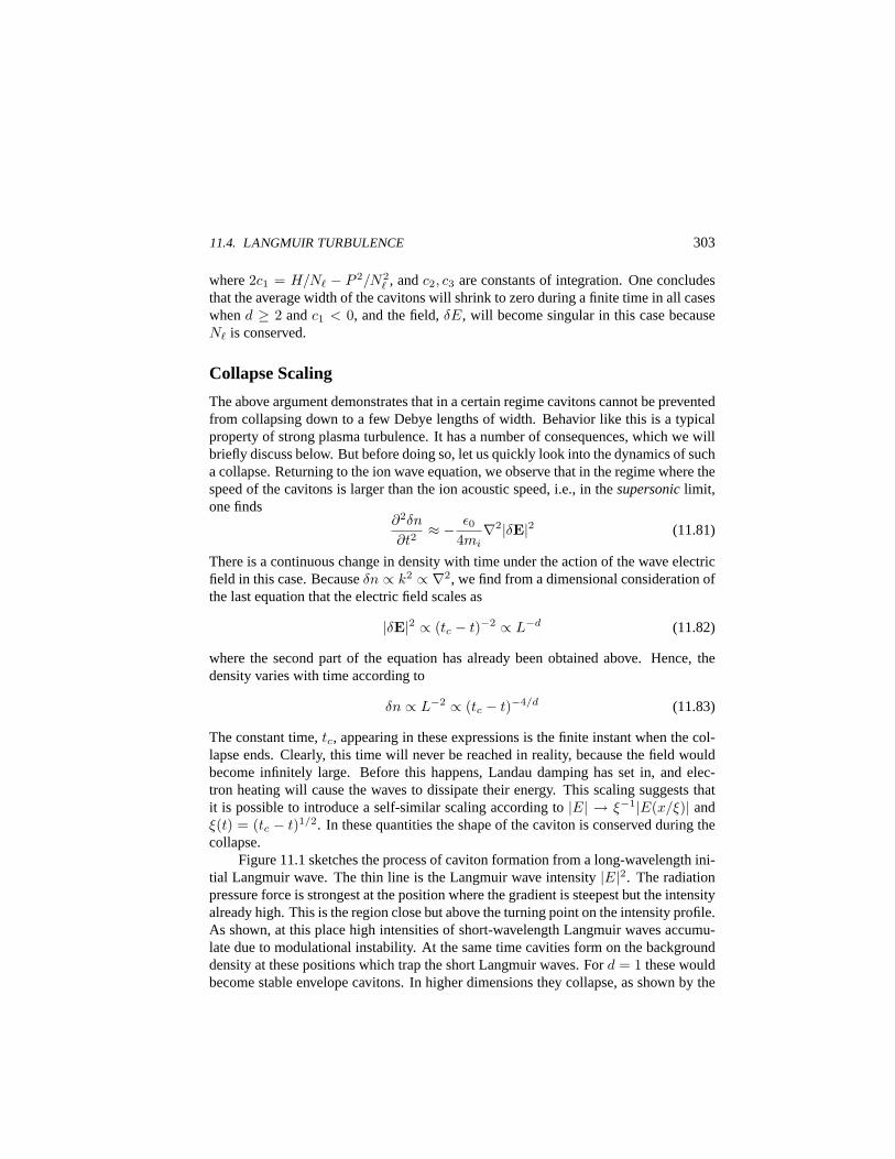
11.4. LANGMUIR TURBULENCE 303
where2c1 = H/N` − P 2/N2` , andc2, c3 are constants of integration. One concludes
that the average width of the cavitons will shrink to zero during a finite time in all caseswhend ≥ 2 andc1 < 0, and the field,δE, will become singular in this case becauseN` is conserved.
Collapse Scaling
The above argument demonstrates that in a certain regime cavitons cannot be preventedfrom collapsing down to a few Debye lengths of width. Behavior like this is a typicalproperty of strong plasma turbulence. It has a number of consequences, which we willbriefly discuss below. But before doing so, let us quickly look into the dynamics of sucha collapse. Returning to the ion wave equation, we observe that in the regime where thespeed of the cavitons is larger than the ion acoustic speed, i.e., in thesupersoniclimit,one finds
∂2δn
∂t2≈ − ε0
4mi∇2|δE|2 (11.81)
There is a continuous change in density with time under the action of the wave electricfield in this case. Becauseδn ∝ k2 ∝ ∇2, we find from a dimensional consideration ofthe last equation that the electric field scales as
|δE|2 ∝ (tc − t)−2 ∝ L−d (11.82)
where the second part of the equation has already been obtained above. Hence, thedensity varies with time according to
δn ∝ L−2 ∝ (tc − t)−4/d (11.83)
The constant time,tc, appearing in these expressions is the finite instant when the col-lapse ends. Clearly, this time will never be reached in reality, because the field wouldbecome infinitely large. Before this happens, Landau damping has set in, and elec-tron heating will cause the waves to dissipate their energy. This scaling suggests thatit is possible to introduce a self-similar scaling according to|E| → ξ−1|E(x/ξ)| andξ(t) = (tc − t)1/2. In these quantities the shape of the caviton is conserved during thecollapse.
Figure 11.1 sketches the process of caviton formation from a long-wavelength ini-tial Langmuir wave. The thin line is the Langmuir wave intensity|E|2. The radiationpressure force is strongest at the position where the gradient is steepest but the intensityalready high. This is the region close but above the turning point on the intensity profile.As shown, at this place high intensities of short-wavelength Langmuir waves accumu-late due to modulational instability. At the same time cavities form on the backgrounddensity at these positions which trap the short Langmuir waves. Ford = 1 these wouldbecome stable envelope cavitons. In higher dimensions they collapse, as shown by the
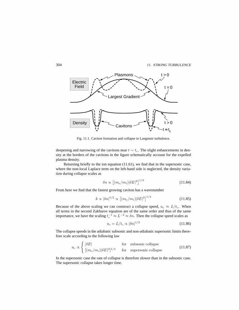
304 11. STRONG TURBULENCE
Largest Gradient
Cavitons
t = 0
Plasmons
Electric Field
Density
t > 0
t > 0
t ≈ tc
Fig. 11.1. Caviton formation and collapse in Langmuir turbulence.
deepening and narrowing of the cavitons neart ∼ tc. The slight enhancements in den-sity at the borders of the cavitons in the figure schematically account for the expelledplasma density.
Returning briefly to the ion equation (11.61), we find that in the supersonic case,where the non-local Laplace term on the left-hand side is neglected, the density varia-tion during collapse scales as
δn ∝ [(me/mi)|δE|2
]1/2(11.84)
From here we find that the fastest growing caviton has a wavenumber
k ∝ |δn|1/2 ∝ [(me/mi)|δE|2
]1/4(11.85)
Because of the above scaling we can construct a collapse speed,uc ≈ L/tc. Whenall terms in the second Zakharov equation are of the same order and thus of the sameimportance, we have the scalingt−1
c ≈ L−2 ≈ δn. Then the collapse speed scales as
uc = L/tc ∝ |δn|1/2 (11.86)
The collapse speeds in the adiabatic subsonic and non-adiabatic supersonic limits there-fore scale according to the following law
uc ∝|δE| for subsonic collapse
[(me/mi)|δE|2]1/4 for supersonic collapse(11.87)
In the supersonic case the rate of collapse is therefore slower than in the subsonic case.The supersonic collapse takes longer time.
11.5. LOWER-HYBRID TURBULENCE 305
11.5. Lower-Hybrid Turbulence
Langmuir waves are only one example of modulational instability, caviton formationand collapse. A large number of other waves may experience the same or similar fate.Among those waves are kinetic Alfven waves, magnetosonic waves, electromagneticcavitons driven by intense laser and maser pulses, whistler waves in weakly magnetizedplasmas, and, as a particularly important application, lower-hybrid waves.
Musher-Sturman Equations
Lower-hybrid waves have the particular property that they propagate perpendicular tothe magnetic field and are intrinsically two-dimensional. As a consequence, the waveradiation pressure becomes an anisotropic tensor, and the ponderomotive forces par-allel and perpendicular to the magnetic field are different. The equations describingstrong lower-hybrid turbulence are not as simple as the Zakharov equations (11.65). Inparticular, the parabolic equation cannot be written in the simple form of a cubic non-linear Schrodinger equation. This is obvious from a first glance at the linear dispersionrelation of lower hybrid waves
ω = ωlh
(1 +
R2k2
2+
mi
2me
k2‖
k2− ω2
pe
k2c2
ω2pe
ω2pe + ω2
ge
)(11.88)
where the quantityR is a typical dispersion length of lower-hybrid waves
R2 =3kBTi
miω2lh
+2kBTe
meω2ge
ω2pe
ω2ge + ω2
pe
(11.89)
which in the case of a dense plasma withωpe À ωge is the electron gyroradius.If one takes the variation of the frequency in the same way as we did in strong
Langmuir turbulence, the resulting expression contains variations with respect to den-sity, δn, magnetic field,δB, and terms containing the parallel, perpendicular, and fullwavenumbers. Interpreting the latter components as operators in space, the resultingequations contain complicated and mixed derivatives of the electric field vector,E, inall directions. One may, however, introduce a number of approximations. The simplestone is the assumption that the wave field is purely electrostatic and that the electric fielddrifts contribute most. In this case the electric field obeys the following set of equations
(∂2
∂t2− c2
ia∇2
)δn =
iε04mi
ω2pe
ωgeωlh∇2 (∇δφ∗ ×∇δφ)‖
(2i
ωlh∇2 ∂
∂t+ R2∇4 − mi
me∇2‖ −
mi
me
ω2pe
c2
ω2lh
ω2ge
)δφ =
i
n0
mi
me
ωlh
ωge(∇δφ×∇δn)‖
(11.90)
306 11. STRONG TURBULENCE
These equations are written in terms of the electric wave potential,δφ, instead of theelectric field,δE. They are calledMusher-Sturman equationsand govern strong lower-hybrid turbulence and lower-hybrid collapse.
Lower-Hybrid Collapse Scaling
The Musher-Sturman equations (11.90) are written in terms of the wave potential andthe density variation in the background. The latter is simply the ion-acoustic waveequation as before, but takes into account the anisotropy. The cross-products appearbecauseE×B motions and polarization motions are important in the lower-hybridwave. Solving these equations is much more difficult than in the Langmuir cavitoncase. But it can also be shown that their solutions yield cavitons, which are formed bymodulational instability. The cavitons turn out to be two-dimensional structures, whichform cigars or pancakes of transverse and parallel lengths
L⊥ ≈ R
[αme
2mi
n0kB(Te + Ti)Wlh
]1/2
L‖ ≈ L2⊥
R
(mi
me
)1/2 (11.91)
Hence, these cavitons are elongated along the magnetic field but propagate at the ion-acoustic velocity. They also experience self-similar collapse which can be described byself-similar formulae. The threshold for modulational instability and caviton formationis given by
WE
n0kB(Te + Ti)≈ 2∆0
(1 +
k2
k20
) (1 +
ω2pe
ω2ge
)−1
(11.92)
The abbreviations used are
∆0 =12
(R2k2 − αω2
pe
k2c2 + k20c
2+
αω2pe
k20c
2+
mi
me
k2‖
k2 + k20
)(11.93)
andα = (1 + ω2ge/ω2
pe)−1. This threshold condition shows that the threshold is fairly
low for lower-hybrid waves and that they can easily reach the regime of modulationalinstability. Once the threshold given in Eq. (11.92) is exceeded, lower-hybrid waves willinevitably undergo modulational instability, caviton formation and collapse in a waysimilar to Langmuir turbulence. But this collapse is two-dimensional and anisotropicand shows a number of differences when compared with Langmuir collapse.
In case of collapse, the length scales of the caviton become functions of the waveintensity, and the time of caviton formation is equal to the inverse growth rate of the

11.6. PARTICLE EFFECTS 307
modulation of the lower-hybrid wave,tmod ∝ γ−1mod, where
γmod ≈ ωlhmi
me
(1 +
ω2pe
ω2ge
)WE
2n0kB(Te + Ti)(11.94)
If one considers the self-similar evolution, one finds from the basic equations that thedensity evolves asδn ∝ (tc − t)−1, while the speed of the collapse, which has beendefined above for Langmuir waves, isuc ∝ (tc − t)−1/2.
11.6. Particle Effects
So far we have neglected the effects on the particles and how the reaction of these par-ticles affects the evolution of the collapse. Before performing some relevant estimateslet us explain the physics of this interaction.
Langmuir Turbulence Effects
The Zakharov equations with the ion wave equation (11.61) and the nonlinear Schro-dinger equation (11.65) describe the localized excitation of ion-acoustic waves form-ing cavitons and the trapping of short-wavelength Langmuir waves in these cavitonsunder the action of the Langmuir wave radiation pressure. The initial state is a long-wavelength Langmuir pump wave, excited presumably by a gentle beam instability.
As the linear theory of the gentle beam instability suggests, Langmuir modes ofthis kind are resonant with the positive slope part of the beam. Such waves may becomescattered at background cold ions in the plasma, in which process they transfer a largepart of their momentum to the ions. This scattering is symbolically described by
` + i → `′ + i′ (11.95)
where` stands for the Langmuir wave,i stands for the ion, and a prime indicates scat-tered products. In particular, for the wavenumber this equation reads
hk` + pi → hk′` + p′i (11.96)
Since the momentum,hk`, of a wave is proportional to its wavenumber,k, loss ofmomentum implies increase of the Langmuir wavelength and decreasing wavenumber.The Langmuir spectrum, in the course of many scattering events, cascades down to lowk.
This implies that the phase velocity of the scattered wave,ω/k, increases consid-erably, and the waves shift out of resonance to high velocities, where no particles existwhich could Landau damp the waves. This scenario is depicted in Fig. 11.2. Clearly
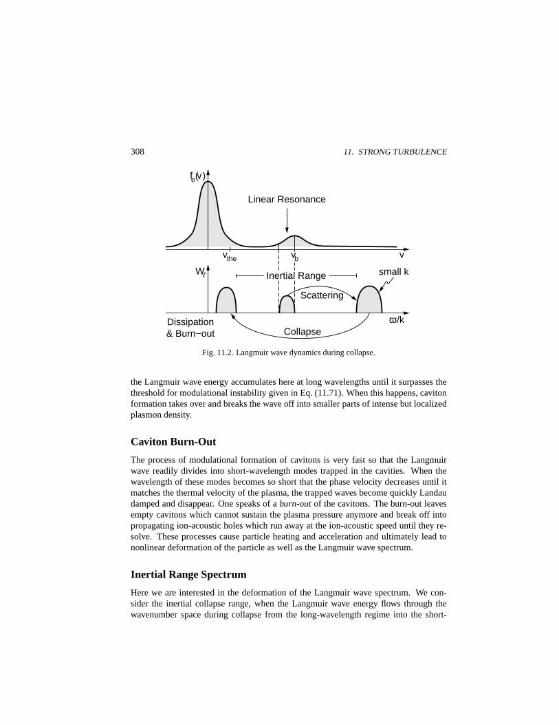
308 11. STRONG TURBULENCE
fe(v)
W
vthe vb
Scattering
Collapse Dissipation & Burn−out
small k
Linear Resonance
v
ω /k
Inertial Range
Fig. 11.2. Langmuir wave dynamics during collapse.
the Langmuir wave energy accumulates here at long wavelengths until it surpasses thethreshold for modulational instability given in Eq. (11.71). When this happens, cavitonformation takes over and breaks the wave off into smaller parts of intense but localizedplasmon density.
Caviton Burn-Out
The process of modulational formation of cavitons is very fast so that the Langmuirwave readily divides into short-wavelength modes trapped in the cavities. When thewavelength of these modes becomes so short that the phase velocity decreases until itmatches the thermal velocity of the plasma, the trapped waves become quickly Landaudamped and disappear. One speaks of aburn-outof the cavitons. The burn-out leavesempty cavitons which cannot sustain the plasma pressure anymore and break off intopropagating ion-acoustic holes which run away at the ion-acoustic speed until they re-solve. These processes cause particle heating and acceleration and ultimately lead tononlinear deformation of the particle as well as the Langmuir wave spectrum.
Inertial Range Spectrum
Here we are interested in the deformation of the Langmuir wave spectrum. We con-sider the inertial collapse range, when the Langmuir wave energy flows through thewavenumber space during collapse from the long-wavelength regime into the short-
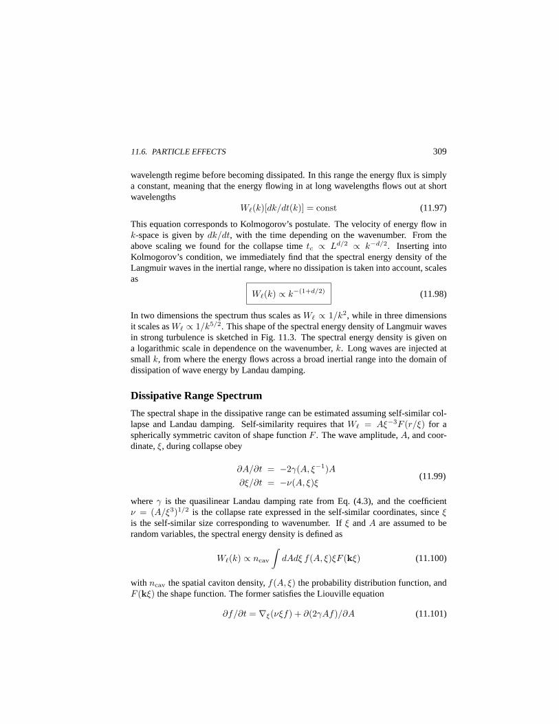
11.6. PARTICLE EFFECTS 309
wavelength regime before becoming dissipated. In this range the energy flux is simplya constant, meaning that the energy flowing in at long wavelengths flows out at shortwavelengths
W`(k)[dk/dt(k)] = const (11.97)
This equation corresponds to Kolmogorov’s postulate. The velocity of energy flow ink-space is given bydk/dt, with the time depending on the wavenumber. From theabove scaling we found for the collapse timetc ∝ Ld/2 ∝ k−d/2. Inserting intoKolmogorov’s condition, we immediately find that the spectral energy density of theLangmuir waves in the inertial range, where no dissipation is taken into account, scalesas
W`(k) ∝ k−(1+d/2) (11.98)
In two dimensions the spectrum thus scales asW` ∝ 1/k2, while in three dimensionsit scales asW` ∝ 1/k5/2. This shape of the spectral energy density of Langmuir wavesin strong turbulence is sketched in Fig. 11.3. The spectral energy density is given ona logarithmic scale in dependence on the wavenumber,k. Long waves are injected atsmallk, from where the energy flows across a broad inertial range into the domain ofdissipation of wave energy by Landau damping.
Dissipative Range Spectrum
The spectral shape in the dissipative range can be estimated assuming self-similar col-lapse and Landau damping. Self-similarity requires thatW` = Aξ−3F (r/ξ) for aspherically symmetric caviton of shape functionF . The wave amplitude,A, and coor-dinate,ξ, during collapse obey
∂A/∂t = −2γ(A, ξ−1)A∂ξ/∂t = −ν(A, ξ)ξ
(11.99)
whereγ is the quasilinear Landau damping rate from Eq. (4.3), and the coefficientν = (A/ξ3)1/2 is the collapse rate expressed in the self-similar coordinates, sinceξis the self-similar size corresponding to wavenumber. Ifξ andA are assumed to berandom variables, the spectral energy density is defined as
W`(k) ∝ ncav
∫dAdξ f(A, ξ)ξF (kξ) (11.100)
with ncav the spatial caviton density,f(A, ξ) the probability distribution function, andF (kξ) the shape function. The former satisfies the Liouville equation
∂f/∂t = ∇ξ(νξf) + ∂(2γAf)/∂A (11.101)
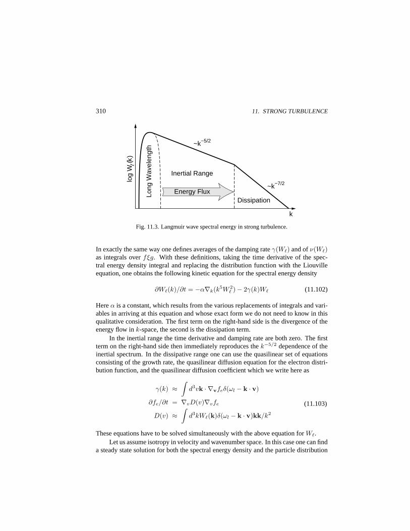
310 11. STRONG TURBULENCE
Long
Wav
elen
gth
Inertial Range
Dissipation
~k−7/2
k
~k−5/2
log
W (k
)
Energy Flux
Fig. 11.3. Langmuir wave spectral energy in strong turbulence.
In exactly the same way one defines averages of the damping rateγ(W`) and ofν(W`)as integrals overfξg. With these definitions, taking the time derivative of the spec-tral energy density integral and replacing the distribution function with the Liouvilleequation, one obtains the following kinetic equation for the spectral energy density
∂W`(k)/∂t = −α∇k(k5W 2` )− 2γ(k)W` (11.102)
Hereα is a constant, which results from the various replacements of integrals and vari-ables in arriving at this equation and whose exact form we do not need to know in thisqualitative consideration. The first term on the right-hand side is the divergence of theenergy flow ink-space, the second is the dissipation term.
In the inertial range the time derivative and damping rate are both zero. The firstterm on the right-hand side then immediately reproduces thek−5/2 dependence of theinertial spectrum. In the dissipative range one can use the quasilinear set of equationsconsisting of the growth rate, the quasilinear diffusion equation for the electron distri-bution function, and the quasilinear diffusion coefficient which we write here as
γ(k) ≈∫
d3vk · ∇vfeδ(ωl − k · v)
∂fe/∂t = ∇vD(v)∇vfe
D(v) ≈∫
d3kW`(k)δ(ωl − k · v)kk/k2
(11.103)
These equations have to be solved simultaneously with the above equation forW`.Let us assume isotropy in velocity and wavenumber space. In this case one can find
a steady state solution for both the spectral energy density and the particle distribution
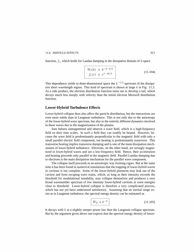
11.6. PARTICLE EFFECTS 311
function,fe, which holds for Landau damping in the dissipative domain ofk-space
W`(k) ∝ k−2−d/2
fe(v) ∝ v1−3d/2(11.104)
This dependence yields in three-dimensional space thek−7/2 spectrum of the dissipa-tive short wavelength region. This kind of spectrum is shown at largek in Fig. 11.3.As a side product, the electron distribution function turns out to develop a tail, whichdecays much less steeply with velocity than the initial electron Maxwell distributionfunction.
Lower-Hybrid Turbulence Effects
Lower-hybrid collapse does also affect the particle distribution, but the interactions areeven more subtle than in Langmuir turbulence. This is not only due to the anisotropyof the lower-hybrid wave spectrum, but also to the entirely different dynamics involvedin these waves due to the magnetization of the plasma.
Ions behave unmagnetized and observe a wave field, which is a high-frequencyfield on their time scales. In such a field they can readily be heated. However, be-cause the wave field is predominantly perpendicular to the magnetic field with only asmall parallel electric field component, ion heating is predominantly transverse. Thistransverse heating implies transverse damping and is one of the main dissipation mech-anisms of lower-hybrid turbulence. Electrons, on the other hand, are strongly magne-tized in lower-hybrid waves and see a low-frequency field. Hence, their accelerationand heating proceeds only parallel to the magnetic field. Parallel Landau damping dueto electrons is the main dissipation mechanism for the parallel wave component.
The collapse itself proceeds in an anisotropic way forming cigars. But at the sametime it has been found in numerical simulations that the trapping of lower-hybrid wavesin cavitons is not complete. Some of the lower-hybrid plasmons may leak out of thecaviton and form escaping wave trains, which, as long as their intensity exceeds thethreshold for modulational instability, may collapse themselves and produces a verybroad wavenumber spectrum of low intensity lower-hybrid cavitons at wave energiesclose to threshold. Lower-hybrid collapse is therefore a very complicated process,which has not yet been understood satisfactory. Assuming that an inertial range ex-ists as in Langmuir turbulence, the spectral energy density can be estimated as
WE ∝ k−3 (11.105)
It decays withk at a slightly steeper power law than the Langmuir collapse spectrum.But by the argument given above one expects that the spectral energy density of lower-
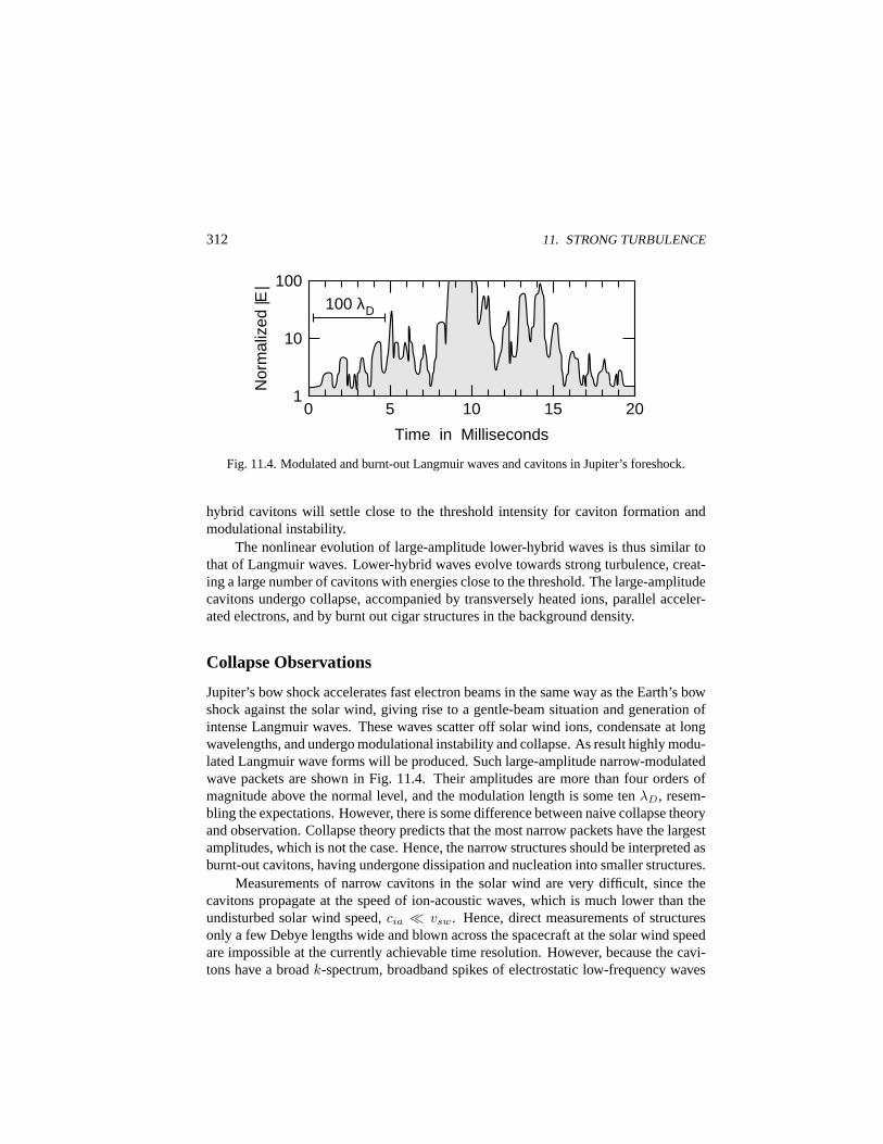
312 11. STRONG TURBULENCE
0 5 10 15 20
Time in Milliseconds
100 λD
1
10
100 N
orm
aliz
ed |E
|
Fig. 11.4. Modulated and burnt-out Langmuir waves and cavitons in Jupiter’s foreshock.
hybrid cavitons will settle close to the threshold intensity for caviton formation andmodulational instability.
The nonlinear evolution of large-amplitude lower-hybrid waves is thus similar tothat of Langmuir waves. Lower-hybrid waves evolve towards strong turbulence, creat-ing a large number of cavitons with energies close to the threshold. The large-amplitudecavitons undergo collapse, accompanied by transversely heated ions, parallel acceler-ated electrons, and by burnt out cigar structures in the background density.
Collapse Observations
Jupiter’s bow shock accelerates fast electron beams in the same way as the Earth’s bowshock against the solar wind, giving rise to a gentle-beam situation and generation ofintense Langmuir waves. These waves scatter off solar wind ions, condensate at longwavelengths, and undergo modulational instability and collapse. As result highly modu-lated Langmuir wave forms will be produced. Such large-amplitude narrow-modulatedwave packets are shown in Fig. 11.4. Their amplitudes are more than four orders ofmagnitude above the normal level, and the modulation length is some tenλD, resem-bling the expectations. However, there is some difference between naive collapse theoryand observation. Collapse theory predicts that the most narrow packets have the largestamplitudes, which is not the case. Hence, the narrow structures should be interpreted asburnt-out cavitons, having undergone dissipation and nucleation into smaller structures.
Measurements of narrow cavitons in the solar wind are very difficult, since thecavitons propagate at the speed of ion-acoustic waves, which is much lower than theundisturbed solar wind speed,cia ¿ vsw. Hence, direct measurements of structuresonly a few Debye lengths wide and blown across the spacecraft at the solar wind speedare impossible at the currently achievable time resolution. However, because the cavi-tons have a broadk-spectrum, broadband spikes of electrostatic low-frequency waves
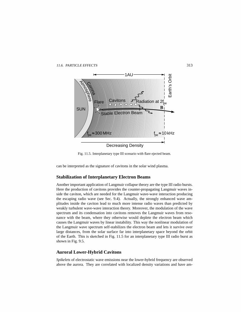
11.6. PARTICLE EFFECTS 313
Flare
fpe ≈ 300 MHz
B
Ear
th’s
Orb
it
Stable Electron Beam
Corona
Atmosphere
1AU
Decreasing Density
fpe ≈ 10 kHz
SUN
Cavitons Radiation at 2fpe
Fig. 11.5. Interplanetary type III scenario with flare ejected beam.
can be interpreted as the signature of cavitons in the solar wind plasma.
Stabilization of Interplanetary Electron Beams
Another important application of Langmuir collapse theory are the type III radio bursts.Here the production of cavitons provides the counter-propagating Langmuir waves in-side the caviton, which are needed for the Langmuir wave-wave interaction producingthe escaping radio wave (see Sec. 9.4). Actually, the strongly enhanced wave am-plitudes inside the caviton lead to much more intense radio waves than predicted byweakly turbulent wave-wave interaction theory. Moreover, the modulation of the wavespectrum and its condensation into cavitons removes the Langmuir waves from reso-nance with the beam, where they otherwise would deplete the electron beam whichcauses the Langmuir waves by linear instability. This way the nonlinear modulation ofthe Langmuir wave spectrum self-stabilizes the electron beam and lets it survive overlarge distances, from the solar surface far into interplanetary space beyond the orbitof the Earth. This is sketched in Fig. 11.5 for an interplanetary type III radio burst asshown in Fig. 9.5.
Auroral Lower-Hybrid Cavitons
Spikeletsof electrostatic wave emissions near the lower-hybrid frequency are observedabove the aurora. They are correlated with localized density variations and have am-
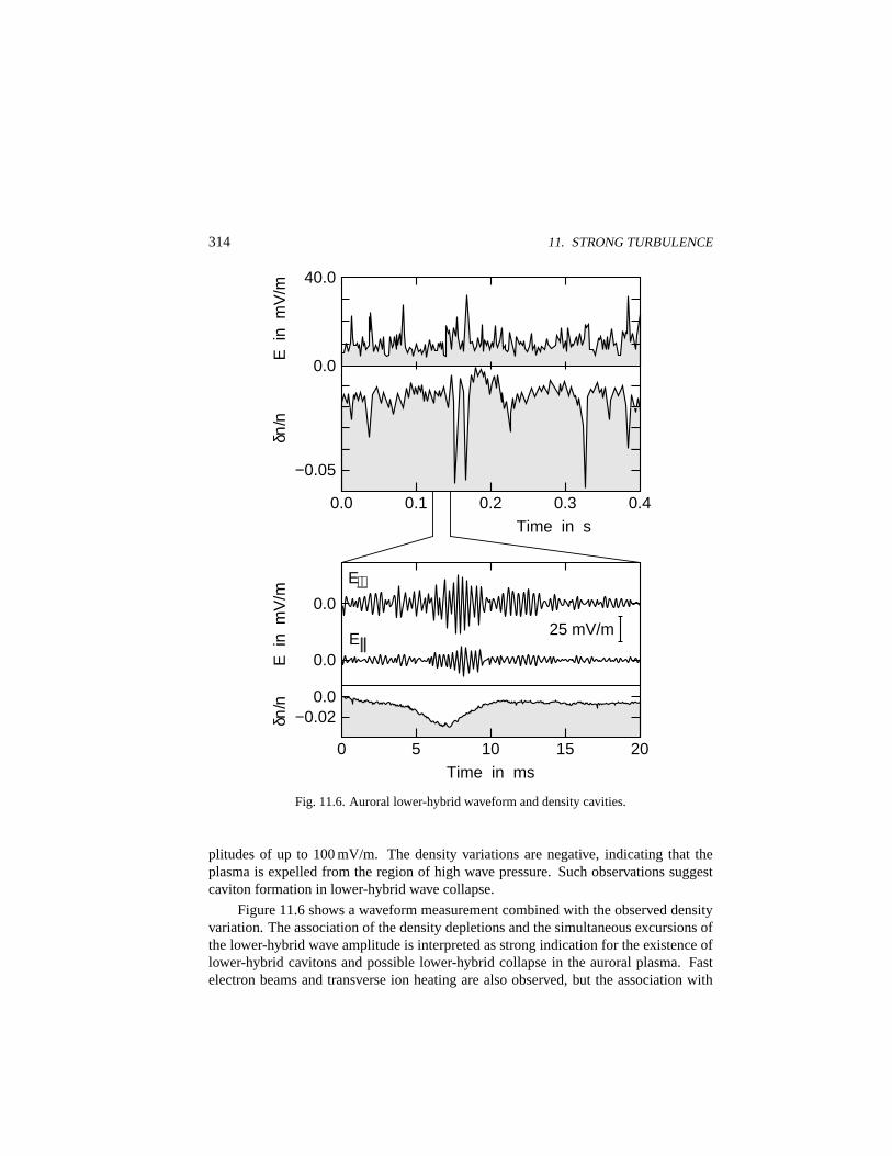
314 11. STRONG TURBULENCE
0.0
−0.05
E i
n m
V/m
δn
/n
0.0 0.2 0.4
0.0
0.0
0.0 −0.02
0 5 10 15 20
E i
n m
V/m
25 mV/m
E⊥
E||
0.1 0.3
Time in ms
Time in s
40.0 δn
/n
Fig. 11.6. Auroral lower-hybrid waveform and density cavities.
plitudes of up to 100 mV/m. The density variations are negative, indicating that theplasma is expelled from the region of high wave pressure. Such observations suggestcaviton formation in lower-hybrid wave collapse.
Figure 11.6 shows a waveform measurement combined with the observed densityvariation. The association of the density depletions and the simultaneous excursions ofthe lower-hybrid wave amplitude is interpreted as strong indication for the existence oflower-hybrid cavitons and possible lower-hybrid collapse in the auroral plasma. Fastelectron beams and transverse ion heating are also observed, but the association with
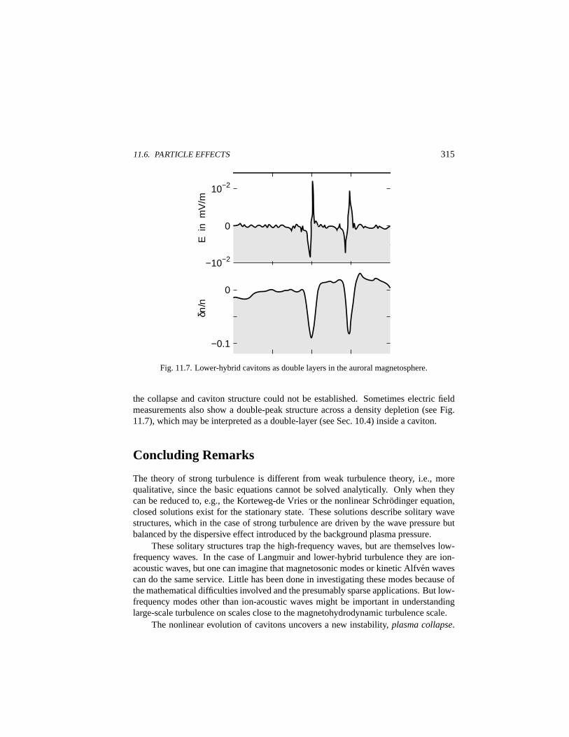
11.6. PARTICLE EFFECTS 315
E i
n m
V/m
10−2
0
−10−2
0
−0.1
δn/n
Fig. 11.7. Lower-hybrid cavitons as double layers in the auroral magnetosphere.
the collapse and caviton structure could not be established. Sometimes electric fieldmeasurements also show a double-peak structure across a density depletion (see Fig.11.7), which may be interpreted as a double-layer (see Sec. 10.4) inside a caviton.
Concluding Remarks
The theory of strong turbulence is different from weak turbulence theory, i.e., morequalitative, since the basic equations cannot be solved analytically. Only when theycan be reduced to, e.g., the Korteweg-de Vries or the nonlinear Schrodinger equation,closed solutions exist for the stationary state. These solutions describe solitary wavestructures, which in the case of strong turbulence are driven by the wave pressure butbalanced by the dispersive effect introduced by the background plasma pressure.
These solitary structures trap the high-frequency waves, but are themselves low-frequency waves. In the case of Langmuir and lower-hybrid turbulence they are ion-acoustic waves, but one can imagine that magnetosonic modes or kinetic Alfven wavescan do the same service. Little has been done in investigating these modes because ofthe mathematical difficulties involved and the presumably sparse applications. But low-frequency modes other than ion-acoustic waves might be important in understandinglarge-scale turbulence on scales close to the magnetohydrodynamic turbulence scale.
The nonlinear evolution of cavitons uncovers a new instability,plasma collapse.
316 11. STRONG TURBULENCE
During collapse the plasma pressure cannot balance the pressure of the wave field,and the plasma is expelled from the region until the wavelength of the trapped wavesbecomes so short that dissipation sets in and the wave field burns out. Collapse maytherefore provide the basic mechanism for dissipation of wave energy out of resonance.It causes localized plasma heating and particle acceleration and redistributes energy.
Further Reading
The theory of modulation of large-amplitude waves can be found in [8]. In the deriva-tion of the nonlinear parabolic equation we used [3]. The nonlinear Schrodinger equa-tion is given in [1], [2], [4], and many other books. A short account of modulationalinstability is found in [2]. The ponderomotive force is derived in the magnetohydrody-namic approximation by Karpman and Washimi,J. Plasma Phys., 18 (1977) 173. Thebriefest reference for the theory of strong Langmuir turbulence is Sagdeev,Rev. Mod.Phys., 51 (1979) 1. Waves in the foreshock region and reports on strong turbulence aregiven in [5] and [7]. The observation of Langmuir wave packets is taken from Gurnettet al.,J. Geophys. Res., 86 (1981) 8833. Formation of shock waves in nonlinear waveevolution is found in [6]. In lower-hybrid collapse theory we followed Shapiro et al.,Phys. Fluids B, 5 (1993) 3148. The measurements of lower-hybrid cavitons are takenfrom Eriksson et al.,Geophys. Res. Lett., 21 (1994) 1843, and Dovner et al.,Geophys.Res. Lett., 21 (1994) 1827.
[1] R. C. Davidson,Methods in Nonlinear Plasma Theory(Academic Press, New York,1972).
[2] A. Hasegawa,Plasma Instabilities and Nonlinear Effects(Springer Verlag, Heidel-berg, 1975).
[3] V. I. Karpman,Nichtlineare Wellen in dispersiven Medien(Vieweg Verlag, Braun-schweig, 1977).
[4] D. R. Nicholson,Introduction to Plasma Theory(Wiley, New York, 1983).
[5] R. G. Stone and B. T. Tsurutani (eds.),Collisionless Shocks in the Heliosphere: ATutorial Review(American Geophysical Union, Washington, 1985).
[6] D. A. Tidman and N. A. Krall,Shock Waves in Collisionless Plasmas(Wiley Inter-science, New York, 1971).
[7] B. T. Tsurutani and R. G. Stone (eds.),Collisionless Shocks in the Heliosphere:Reviews of Current Research(American Geophysical Union, Washington, 1985).
[8] G. B. Whitham,Linear and Nonlinear Waves(Wiley, New York, 1974).
12. Collective Effects
In this last chapter we consider three special types of collective interactions, the gen-eration of anomalous collisions and diffusion in an otherwise collisionless plasma, col-lisionless shock waves, and the acceleration of plasma particles to high energies. Thisselection of topics is guided by practical needs in space physics. Of course, all chap-ters of this book include collective effects. But the present chapter selects those effectswhich fall somewhat outside the main course of the theory-oriented presentation, whichproceeded from linear instability to the nonlinear processes.
The first effect, anomalous collisions, is probably the most important macroscopiceffect in a collisionless plasma. It is caused by close correlations between the parti-cles, which replace the two-body collisions in ordinary collision-dominated systems.Binary collisions let collisional systems evolve towards relaxation and equilibrium andallow for a macroscopic description in terms of a fluid theory. In a collisionless plasmathere are no binary collisions. Instead the collisions are replaced by interactions be-tween the particles and various kinds of waves, which are responsible for relaxationprocesses in collisionless plasmas and ultimately justify the use of a fluid description.The immediate consequence of anomalous collisions is anomalous plasma resistivity,the appearance of finite relaxation times, and plasma diffusivity. These enter the phe-nomenological fluid equations of the plasma as transport coefficients and lead to itsnon-ideality.
Collisionless shock waves, the second collective effect selected, play a dominantrole in many fast flows encountered in space. Since the magnetosphere including itsdynamics is the result of the interaction of the fast solar wind flow with the geomagneticfield as an obstacle, the investigation of the processes at bow shock is of vital interest.Shock physics can be studied in situ by investigating its properties. Many of the resultshave been extrapolated to other shocks in the solar system and astrophysical objects.
The last collective effect treated in this chapter is particle acceleration in collision-less plasmas, leading to particle heating and particle beams. We discuss a number ofconditions under which such acceleration can appear. This discussion is by no meansexhaustive nor even complete. Only some basic acceleration processes are sketched.
317

318 12. COLLECTIVE EFFECTS
12.1. Anomalous Resistivity
The determination of transport coefficients is one of the most important aspects of mi-croscopic theory. Measured quantities, like density, flow velocity, and temperature, areusually of macroscopic nature. These quantities are mutually related through macro-scopic conservation laws or evolution equations. The latter are derived from the mi-croscopic equations, as demonstrated in Chap. 7 of our companion book,Basic SpacePlasma Physics. In collisionless plasmas, the absence of collision and correlation termsin the Vlasov equation corresponds to a lack of transport coefficients and, hence, to theabsence of any obvious irreversible effects. Transport of a macroscopic quantity in thiscase proceeds by convection. This means that only macroscopic motions like flow andwave propagation lead to transport.
In such a case there would be no energy exchange, and in reality this is not pos-sible. We have learned that instabilities arise and that irreversible processes may existin a collision-free plasma. The irreversible processes are a consequence of nonlinearinteractions between the fields and particles. Viewed from a macroscopic position, theyproduce transport coefficients which are calledanomalous, because they arise fromthese pseudo-collisions. These pseudo-collisions are a result of the property of theVlasov equation to generate unstable and irreversible interactions between fields andparticles, which can formally be reflected in the appearance of an average correlationterm on the right-hand side of the general quasilinear equation (8.38).
Determination of anomalous transport coefficients requires to solve this equationand to derive the macroscopic evolution or transport equations by taking moments ofEq. (8.38). This is a difficult problem. In the present section we give a short account onhow to calculate anomalous resistivities in a plasma under certain restrictive conditions.
Anomalous Collisions
Resistivity is caused by friction. Friction results from collisions between particles.The problem of finding the resistivity is thus reduced to the problem of finding thecollision frequency. Instead of anomalous resistivity one may speak of anomalous col-lision frequencies. How collision frequencies are determined in the collisional casehas been shown in Chap. 4 of our companion book. Let us restrict ourselves to theone-dimensional unmagnetized case and consider the electron equation of motion in anexternal electric field
me dve/dt = −eE −meνve (12.1)
Under stationary conditions the current is defined asj = −en0ve = σE. The electricalresistivity,η = 1/σ, is given by
η = ν/ω2peε0 (12.2)
12.1. ANOMALOUS RESISTIVITY 319
For a collisional plasma, with electron-ion Coulomb collisions dominating the dynam-ics, Eq. (I.4.9) from our companion book suggests that the Spitzer collision frequencycan be expressed as
νei ∝ ωpe
n0λ3D
=ωpeWtf
n0kBTe(12.3)
The classical collision frequency in a plasma thus turns out to be proportional to theenergy density of thermal fluctuations,Wtf in Eq. (2.54), normalized to the thermal en-ergy density of the plasma. One thus realizes that in Coulomb collisions the interactionbetween electrons and ions is mediated by the thermal fluctuation energy stored in theLangmuir wave field, assuming that the plasma is in thermal equilibrium. The collidingelectrons are scattered by the oscillations in the thermal wave field.
This picture is somewhat surprising, but it explains the physical mechanism andmay serve as starting point of a theory of anomalous collisions, since if one can increasethe strength of the wave fluctuation field by some means, e.g., by instability, one alsoenhances the collision frequency. This is the basic idea of the mechanism of anoma-lous collisions. It is of particular importance in plasmas which are so dilute and hotthat Coulomb collisions are spurious, as in the case of most space plasmas. Instabil-ities which saturate the wave fields on a high level, orders of magnitudes higher thanthe thermal fluctuation level, may be responsible for the observed enhanced collisions,dissipation, and transport.
Collisions do not act on electrons and ions in the same way. Electrons are typicallyaffected most. Hence, collision frequencies will always cause currents and the problemof finding self-consistent anomalous collision frequencies becomes the problem of cur-rent instabilities. Initially a sufficiently strong current excites plasma oscillations whichgrow until saturation. At that time the current is either disrupted by strong anomalousresistivity or at least retarded, with the energy of the current transformed into irregularelectron scattering and anomalous Joule heating of the plasma. Thus the anomalousresistivity will heavily depend on the kind of instability, on the instability threshold,and on the strength of the current.
A simple expression for the anomalous collision frequency arising from any linearcurrent instability can be found in a way, which formally duplicates the above derivationof the classical collision frequency. There the collision frequency has been definedimplicitly as the rate of momentum transfer between the electron fluid and the wavefluctuations. In the presence of an unstable current-driven wave spectrum and understationary conditions, when both the instability has saturated and an equilibrium hasbeen established between the friction the electrons experience and the electric forcewhich accelerates them, the momentum transfer is determined by
meνanvde = −eE (12.4)
The momentum on the left-hand side of this equation is transferred to the wave withenergy densityWw. Remember that the wave momentum can be defined as the wave

320 12. COLLECTIVE EFFECTS
energy divided by frequency,ω, and multiplied by wavenumber,k. Thus the change inwave momentum,∆pw, is
∆pw =∫
d3k
8π3
kω(k)
γ(k)Ww(k) (12.5)
In equilibrium between the change in electron momentum and wave momentum, thisexpression gives an estimate of the anomalous collision frequency
νan ≈ 1n0mev2
de
∫d3k
8π3
k · vde
ω(k)γ(k)Ww(k) (12.6)
in terms of the phase velocity of the unstable spectrum, the wave spectral energy density,and the drift velocity of the electrons which provide the electric current. The problemis thus reduced to the problem of finding the saturated spectral density (2.19) of thewaves,Ww(k). The growth rate entering Eq. (12.6) is understood in the quasilinearsense as the growth rate before saturation, but depending on the saturation mechanism.
Let us assume, for example, that we are dealing with the current-driven ion-acoustic instability. The ion-acoustic instability is an electrostatic resonant instabilitywith drifting electrons. The quasilinear equation for the electron distribution functionresponsible for an electrostatic resonant instability can be written as
∂f0e(t)∂t
=e2
8π2m2e
∫d3k k · ∂
∂v
[|δφ(k, t)|2 δ(ω − k · v)k · ∂
∂v
]f0e(t) (12.7)
were δφ(k) is the wave electric potential. We multiply this equation withmv andintegrate over velocity space, using the dispersion relation for ion-acoustic waves. Inthe stationary state the integral over the term on the right-hand side gives the frictionterm
νanmen0vde =1
8π3
∫d3k
kω(k)
γ(k)Ww(k) (12.8)
where we replacedWw = (∂ωε/∂ω)WE . This expression agrees with Eq. (12.6).
Sagdeev Formula
Estimates for the anomalous collision frequencies can be obtained in a particular caseby calculating the saturated wave amplitudes and finding the growth rates. The simplestway is to use the linear maximum growth rates and the wave dispersion relations. Themaximum growth rate for the ion-acoustic instability given in Eq. (4.27) can be used,for instance, to find an estimate for the ion-acoustic anomalous resistivity. As we know,the ion-acoustic wave becomes unstable for current driftsvde > cia. The maximumunstable wavelength is of the order of the Debye length, such thatkmax ≈ 1/λD. We
12.1. ANOMALOUS RESISTIVITY 321
approximateγ ≈ ωvde/vthe for large drifts and find theSagdeev formulafor the ion-acoustic anomalous collision frequency
νia,an ≈ ωpeWw/n0kBTe (12.9)
which leaves us with the determination of the saturation level of ion-acoustic waves.
Buneman Collision Frequency
The Buneman instability is a very strong instability, which must switch off itself whenevolving. Its phase velocity isω/k ≈ vthe
√me/mi, and the wave energy density is
Ww ≤ Wi, less or equal to the ion thermal energy. Hence, the collision frequencyturns out to beνbun,an ≈ ωpi, which is of the order of the ion plasma frequency, thehighest possible frequency of ion-acoustic waves. For example, in the solar wind theion plasma frequency is of the order of 3 kHz. If one compares this with the Spitzercollision frequency of roughly 0.5 collisions per 1 AU, or1.4 · 10−4 Hz, one realizesthat the anomalous collision frequency caused by the Buneman instability is about2·107
times larger than the Spitzer collision frequency.
Ion-Acoustic Collision Frequency
In order to find the ion-acoustic collision frequency, one must calculate the wave sat-uration level, which depends on the mechanism by which the waves saturate. Thereare several possibilities. The instability can saturate quasilinearly, by particle trappingin the wave and subsequent resonance broadening, by wave-wave interaction betweenthe current-driven ion-acoustic wave and Langmuir waves, resulting in escaping radia-tion, by other kinds of wave-wave interactions with Langmuir or lower-hybrid waves,leading to the formation of envelope solitons or cavitons, by nonlinear evolution of theion-acoustic waves into topological solitons, or, finally, by generation of holes in phasespace and hole collisions. Few of these mechanisms have been explored and some ofthem may be unimportant, since the fastest saturation mechanism will in most casesdominate. In particular, single wave effects as particle trapping, topological solitonformation or envelope solitons will be of little importance in broadband ion-acousticturbulence excited by currents at sufficiently large speeds above threshold.
In the weak turbulence approximation the evolution of the wave energy density isdescribed in the simplest case by the evolution equation
∂Ww(k)∂t
=
[2γ(k)−Aω(k)
Ww
n0kBTe−Bω(k)
(Ww
n0kBTe
)2
+ . . .
]Ww(k)
(12.10)
322 12. COLLECTIVE EFFECTS
The different terms in the expansion on the right-hand side of this equation correspondto the quasilinear, three-wave, four-wave interaction, etc. The coefficientsA,B in thisexpression are in fact integral operators describing the different coupling terms con-tributing to the second and third orders in the expansion. Clearly, the mere expansionrequires that the wave energy density is small compared to the plasma energy, thus ex-cluding non-perturbative nonlinearities like solitons. The only process contributing tothe quadratic term is scattering of ion-acoustic waves on ions with the resonance condi-tion ω−ω′ = (k−k′) ·vi. Under stationary conditions the terms on the right-hand sidebalance. Usually one keeps only the two first terms balancing the linear growth rate andthe scattering of waves by ions at very large electron temperatures,Te À Ti, when theion-acoustic instability can develop. It leads to the following anomalous ion-acousticcollision frequency
νan,ia = 0.01 ωpivde
cia
Te
Tiθ−2 (12.11)
where the small factor 0.01 is partially compensated by the large electron-to-ion temper-ature ratio. Also, for large current drift velocities, exceeding the ion-acoustic velocityby far, and for narrow wave scattering angle,θ, the anomalous collision frequency canbecome substantial and of the order of the Buneman collision frequency.
Critical Electric Field
The production of anomalous resistivity by scattering of current-carrying electrons offthe self-excited ion-acoustic waves will reduce the current and thus lead to quasilineareffects and possible reduction of the current, such that the current speed is reduceduntil some equilibrium is reached. This equilibrium depends on the applied electricfield. Quasilinearly the current will saturate at a certain velocity,jcr = −envd,cr.
But when the electric field is very large, larger than another critical value,E =Ecr, the current will again increase, since then fast electrons, therun-away electronpart of the distribution function, start to escape the collisions because of their largemean free paths. Actually, the fast electrons ignore the field fluctuations like a fast carignores the short-length roughness of a street cover.
The electron-ion Spitzer collision frequency is given by
νei = n0σc〈ve〉 (12.12)
where the angular brackets indicate the ensemble average as well as the average overthe electron deflection angle. The Spitzer collisional cross-section (I.4.9) is a functionof the actual electron velocity,ve. It can be written as
σc =ω4
pe
16πn20v
4e
(12.13)

12.1. ANOMALOUS RESISTIVITY 323
Linear Ohm’s Law
Quasilinear Regime
jcr = −en vd,cr
jcr
Ecr
j∝E1/3
Electric Field
Cur
rent
Den
sity
Fig. 12.1. Relation between current and field in a collisionless plasma.
All the electrons with velocities up to the thermal speed,〈ve〉 = vthe, are confined bycollisions. However, for the much faster tail electrons the collision frequency decreasesasv−3
e , such that these electrons become asymptotically free again.For large electric fields and given collision frequency,ν, no equilibrium can be
reached because the acceleration of the electrons by the field is faster than the collisionaldeceleration. The critical electric field above which the electrons become free is easilyfound from the one-dimensional non-relativistic electron equation of motion
medve/dt = −eE −meνve (12.14)
Hence, the marginal field amplitude for equilibrium is given by
Ecr = meνve/e (12.15)
Inserting the Spitzer collision frequency yields theDreicer fieldstrength
ED = e/16πε0λ2D (12.16)
But Eq. (12.15) holds more generally for any anomalous collision frequency. It may beexpressed through the wave intensity using the Sagdeev formula (12.9)
Ecr = Ww/2en0λD (12.17)
324 12. COLLECTIVE EFFECTS
In the ion-acoustic case, the critical electric field is given approximately by
Ecr ≈ 0.01mi
e
(me
mi
)1/4
ωpicia (12.18)
The critical current stays constant for an increasing electric field as long asE < Ecr.But whenE exceedsEcr, the current increases drastically. The increase in the currentaboveEcr is approximatelyj ∝ E1/3. This is shown schematically in Fig. 12.1.
Ion-Cyclotron Collision Frequency
A number of other instabilities can also be excited by currents (see Sec. 4.4). Most im-portant are ion-cyclotron waves excited by field-aligned currents. These waves saturatepredominantly by resonance broadening of the otherwise narrow spectral band (see Sec.8.4), causing the collision frequency to be of the order of a fraction of the ion-cyclotronfrequency
νic,an ≈ 0.25ωgi
(π
2
)1/2 k‖vthe
ωgi(12.19)
This value is clearly much lower than that of the ion-acoustic instability. Nevertheless,anomalous collisions due to ion-cyclotron waves may sometimes be important when thethreshold of the ion-acoustic instability is not exceeded by weak field-aligned currentsand ion-cyclotron waves undergo instability. This may occur in strong magnetic fieldswhen the plasma is underdense,ωpe ¿ ωge, like in the upper auroral ionosphere.
Electron-Cyclotron Collision Frequency
Similar to ion-cyclotron waves, electron-cyclotron waves may also become unstable inthe presence of field-aligned currents. One can imagine that these waves are excitedby the electron beam constituting the current, especially if the current is carried byenergetic electrons. In this case the wave also saturates by resonance broadening.
If the current is carried by the bulk electrons, the current flow will Doppler-shiftthe frequency down toω′ = lωge − k‖vde in the rest frame of the ions, which donot participate in the current flow. Forω′ ≈ k‖vthi the ions can interact with theelectron-cyclotron waves, and a negative energy wave will be excited. This happenseven for low electron temperatures, but saturation of the waves occurs at very smallamplitudes due to trapping and broadening. The wavenumber of the growing waves isaboutk‖ ≈ ωge/vde, and the collision frequency becomes
νec,an ≈ 0.1ωge(vde/vthe)3 (12.20)
12.1. ANOMALOUS RESISTIVITY 325
Because the current drift speed is generally much less than the electron thermal velocity,this value is low. For instance, in the auroral magnetosphere, where this instabilitymight be important, the drift velocity is of the order of the ion-acoustic speed, implyingνec,an ≈ 10−6ωge. The most important region for auroral processes is the excitationregion of auroral kilometric radiation at about 3000 km altitude. There the electron-cyclotron frequency is about 300 kHz. Multiplying with2π one finds that the collisionfrequency becomes not more thanνec,an ≈ 1 Hz, too low to be of any importance.
Lower-Hybrid Drift Collision Frequency
The last instability important for the excitation of anomalous collisions is the lower-hybrid drift instability. The quasilinear saturation level of this instability is given inEq. (8.75). We recall that the lower-hybrid drift instability is caused by transverse cur-rents, not by the field-aligned currents discussed so far. This instability will thereforebe most important for interrupting perpendicular currents, which exist in extended cur-rent layers subject to reconnection. One can expect that it will provide the diffusivityand anomalous resistivity needed to initiate reconnection in such current sheets and todisrupt magnetic fields and release magnetic field energy stored in transverse currents.
Lower-hybrid drift instabilities require density and temperature gradients but arestabilized by magnetic shear which counteracts the density gradients. On the otherhand, plasma streaming may help to destabilize the waves by coupling it to the Kelvin-Helmholtz mode and low-frequency turbulence. However, it is generally believed thatlow-β conditions are needed to keep this instability growing while high-β conditionsshould inhibit its growth. This is true for the excitation of the instability, but if a guidefield is present and the current causes an additional transverse shear in the field, this ar-gument does not apply, because the guide field makes up for the low-β condition whilethe transverse field may in the region of anomalous resistivity merge and reconnect.
The anomalous collision frequency caused by the lower-hybrid drift instability ina dense plasma,ωpe > ωge, can be represented as
νlh,an ≈(π
2
)1/2 ω2pe
ωlh
WE(k⊥,∞)n0kBTi
(12.21)
Using Eq. (8.75) to express the saturation level of the lower-hybrid drift instabilityunder the assumption that saturation proceeds via quasilinear plateau formation, onegets
νlh,an ≈(π
2
)1/2(
rgi
4Ln
)2
ωlh (12.22)
This value is of the order of the lower-hybrid frequency itself. In a strong magneticfield with steep density gradients of the order of the ion gyroradius, it becomes equal
326 12. COLLECTIVE EFFECTS
to the ion plasma frequency. In weaker magnetic fields it is the geometric mean of theelectron- and ion-cyclotron frequencies.
Thatνlh,an becomes proportional to the cyclotron frequency implies that the colli-sion frequency is proportional to the magnetic field. The lower-hybrid drift anomalouscollision frequency will be very important whenever the plasma is able to evolve shortscale density gradients. Such situations are encountered in the auroral magnetosphere,near the magnetopause and the bow shock, and in some regions of the magnetotail.
The critical electric field for the lower-hybrid drift instability, above which elec-trons will escape, can be estimated from the collision frequency, if one assumes that thewaves propagate at a large angle to the magnetic field. In this casek‖/k⊥ ¿ 1, onlythe parallel field plays a role in the confinement, and the critical electric field is givenby
Ecr ≈ mirgi
e
k2‖
k2⊥
(πTe
2Ti
)1/2 (rgi
4Ln
)2
ω2lh (12.23)
Electric fields exceeding this value will readily accelerate the electrons parallel to themagnetic field. However, due to the small angular factor these parallel fields can bequite small. On the other hand, regions of strong lower-hybrid drift wave turbulencemay serve as sources of parallel electron fluxes. Below we will show that in suchregions electrons may be accelerated to substantially high energies fitting into the rangeof auroral electron energies.
Strongly Turbulent Collisions
Anomalous collision frequencies are dominated by the level of wave turbulence. Thelowest level is the thermal fluctuation level, which in the case of Langmuir fluctuationsjust leads to the Spitzer collision frequency given in Eq. 12.12. In the former sectionswe estimated fluctuation levels based on saturation levels of various plasma instabili-ties in weak turbulence. However, in many cases the state of weak turbulence is notreached, and the plasma undergoes modulational instability and switches over to strongturbulence. In strong turbulence the wave spectrum breaks off into a large number ofsolitons and cavitons with heavily modulated background density. Electron-ion colli-sions become considerably more frequent and violent under these conditions, and thecollision frequencies may exceed the quasilinear and weakly turbulent values.
In order to determine the strongly turbulent collision frequencies, one can followthe same line of arguments as before and substitute the strong turbulence level of thecorresponding waves into the Sagdeev formula (12.9). Let us write this formula for astrong turbulence wave level,Wst
νan ≈ αωpe (Wst/n0kBTe) (12.24)
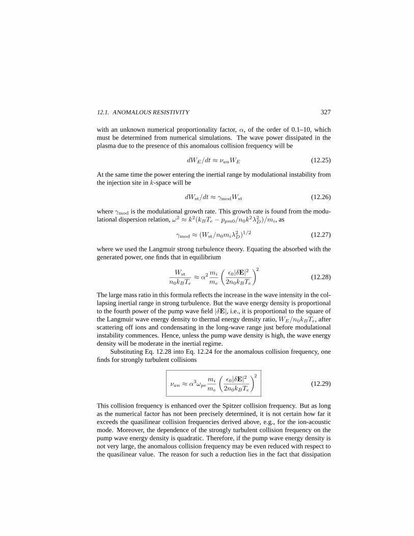
12.1. ANOMALOUS RESISTIVITY 327
with an unknown numerical proportionality factor,α, of the order of 0.1–10, whichmust be determined from numerical simulations. The wave power dissipated in theplasma due to the presence of this anomalous collision frequency will be
dWE/dt ≈ νanWE (12.25)
At the same time the power entering the inertial range by modulational instability fromthe injection site ink-space will be
dWst/dt ≈ γmodWst (12.26)
whereγmod is the modulational growth rate. This growth rate is found from the modu-lational dispersion relation,ω2 ≈ k2(kBTe − ppm0/n0k
2λ2D)/mi, as
γmod ≈ (Wst/n0miλ2D)1/2 (12.27)
where we used the Langmuir strong turbulence theory. Equating the absorbed with thegenerated power, one finds that in equilibrium
Wst
n0kBTe≈ α2 mi
me
(ε0|δE|2
2n0kBTe
)2
(12.28)
The large mass ratio in this formula reflects the increase in the wave intensity in the col-lapsing inertial range in strong turbulence. But the wave energy density is proportionalto the fourth power of the pump wave field|δE|, i.e., it is proportional to the square ofthe Langmuir wave energy density to thermal energy density ratio,WE/n0kBTe, afterscattering off ions and condensating in the long-wave range just before modulationalinstability commences. Hence, unless the pump wave density is high, the wave energydensity will be moderate in the inertial regime.
Substituting Eq. 12.28 into Eq. 12.24 for the anomalous collision frequency, onefinds for strongly turbulent collisions
νan ≈ α3ωpemi
me
(ε0|δE|2
2n0kBTe
)2
(12.29)
This collision frequency is enhanced over the Spitzer collision frequency. But as longas the numerical factor has not been precisely determined, it is not certain how far itexceeds the quasilinear collision frequencies derived above, e.g., for the ion-acousticmode. Moreover, the dependence of the strongly turbulent collision frequency on thepump wave energy density is quadratic. Therefore, if the pump wave energy density isnot very large, the anomalous collision frequency may be even reduced with respect tothe quasilinear value. The reason for such a reduction lies in the fact that dissipation
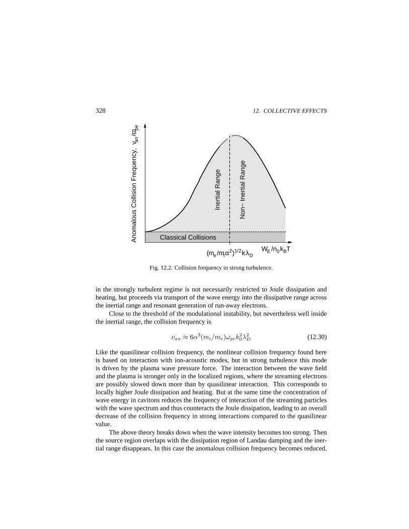
328 12. COLLECTIVE EFFECTS
Classical Collisions
Iner
tial R
ange
Non
− In
ertia
l Ran
ge
WE /n0kBT
Ano
mal
ous
Col
lisio
n F
requ
ency
, ν a
n/ω
pe
(me /miα2)1/2kλD
Fig. 12.2. Collision frequency in strong turbulence.
in the strongly turbulent regime is not necessarily restricted to Joule dissipation andheating, but proceeds via transport of the wave energy into the dissipative range acrossthe inertial range and resonant generation of run-away electrons.
Close to the threshold of the modulational instability, but nevertheless well insidethe inertial range, the collision frequency is
νan ≈ 6α3(mi/me)ωpek20λ
2D (12.30)
Like the quasilinear collision frequency, the nonlinear collision frequency found hereis based on interaction with ion-acoustic modes, but in strong turbulence this modeis driven by the plasma wave pressure force. The interaction between the wave fieldand the plasma is stronger only in the localized regions, where the streaming electronsare possibly slowed down more than by quasilinear interaction. This corresponds tolocally higher Joule dissipation and heating. But at the same time the concentration ofwave energy in cavitons reduces the frequency of interaction of the streaming particleswith the wave spectrum and thus counteracts the Joule dissipation, leading to an overalldecrease of the collision frequency in strong interactions compared to the quasilinearvalue.
The above theory breaks down when the wave intensity becomes too strong. Thenthe source region overlaps with the dissipation region of Landau damping and the iner-tial range disappears. In this case the anomalous collision frequency becomes reduced.

12.2. ANOMALOUS DIFFUSION 329
Figure 12.2 shows the dependence of the anomalous collision frequency on the initialpump wave energy density. The collision frequency increases in the inertial range andpresumably decays when the inertial range disappears for very strong initial wave am-plitudes. The absolute scale can be determined only after the unknown factorα hasbeen determined by numerical simulations.
12.2. Anomalous Diffusion
It is natural to extend the discussion of anomalous collision frequencies to other pro-cesses where collision frequencies play a role. Such processes are thermal conductionand diffusion of matter. Thermal conductivities are known to be inversely proportionalto the collision frequency. Hence, substantial increases in the collision frequency assuggested in the previous section will tend to inhibit thermal conduction and decreasethe heat flux, supporting storage of heat in regions bounded by zones of high anoma-lous collision frequencies. When anomalous collisions arise in regions of strong currentflow, the heat flux from this region will become strongly inhibited, the region will ther-mally decouple from the environment, and will heat up to substantial temperatures. Inregions of field-aligned currents the zone of anomalous collision frequency and resistiv-ity along the magnetic field lines will always become a region of strong plasma heatingand accumulation of heat.
The other important effect is plasma diffusion. Anomalous collision frequenciescause diffusion coefficients to change. Parallel diffusion behaves similar to heat con-ductivity. Since it is defined as
D‖ = kBT/mν (12.31)
use of the anomalous collision frequency in the place ofν indicates that diffusion par-allel to the magnetic field is strongly inhibited in regions of high anomalous collisionfrequency. Particles are trapped in these regions due to the large number of collisionsthey experience. Moreover, ambipolar effects set on and limit the diffusion of bothparticle components to about the diffusivity of the lesser mobile species, thereby main-taining plasma quasineutrality.
For perpendicular diffusion with a diffusion coefficient defined as
D⊥ = D‖/(1 + ω2ge/ν2) (12.32)
no ambipolar diffusion arises, because a transverse electric field can exist in magnetizedplasmas. They simply reflect plasma motions. In strong magnetic fields perpendiculardiffusion is proportional to the anomalous collision frequency and is strongly enhanceddue to the scattering of particles in the wave fields in all directions, which provides atransverse motion of the particles. Classically, the diffusion is known to be inverselyproportional to the square of the magnetic field.
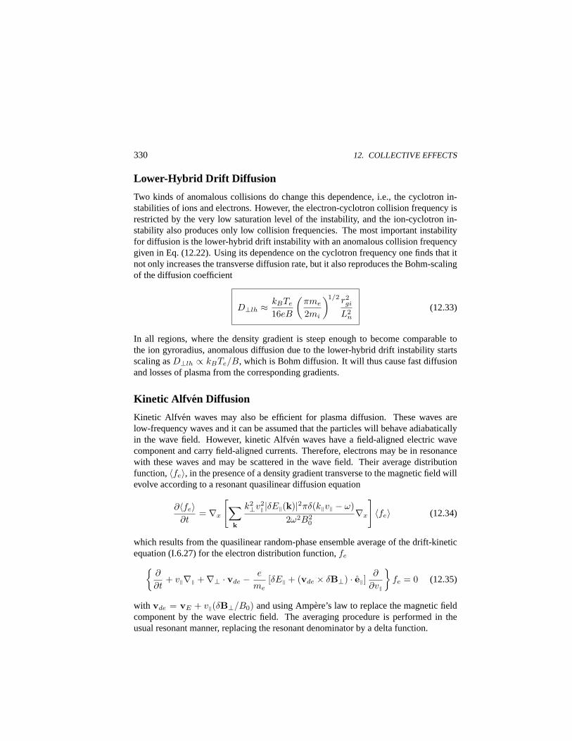
330 12. COLLECTIVE EFFECTS
Lower-Hybrid Drift Diffusion
Two kinds of anomalous collisions do change this dependence, i.e., the cyclotron in-stabilities of ions and electrons. However, the electron-cyclotron collision frequency isrestricted by the very low saturation level of the instability, and the ion-cyclotron in-stability also produces only low collision frequencies. The most important instabilityfor diffusion is the lower-hybrid drift instability with an anomalous collision frequencygiven in Eq. (12.22). Using its dependence on the cyclotron frequency one finds that itnot only increases the transverse diffusion rate, but it also reproduces the Bohm-scalingof the diffusion coefficient
D⊥lh ≈ kBTe
16eB
(πme
2mi
)1/2 r2gi
L2n
(12.33)
In all regions, where the density gradient is steep enough to become comparable tothe ion gyroradius, anomalous diffusion due to the lower-hybrid drift instability startsscaling asD⊥lh ∝ kBTe/B, which is Bohm diffusion. It will thus cause fast diffusionand losses of plasma from the corresponding gradients.
Kinetic Alfv en Diffusion
Kinetic Alfv en waves may also be efficient for plasma diffusion. These waves arelow-frequency waves and it can be assumed that the particles will behave adiabaticallyin the wave field. However, kinetic Alfven waves have a field-aligned electric wavecomponent and carry field-aligned currents. Therefore, electrons may be in resonancewith these waves and may be scattered in the wave field. Their average distributionfunction,〈fe〉, in the presence of a density gradient transverse to the magnetic field willevolve according to a resonant quasilinear diffusion equation
∂〈fe〉∂t
= ∇x
[∑
k
k2⊥v2
‖ |δE‖(k)|2πδ(k‖v‖ − ω)2ω2B2
0
∇x
]〈fe〉 (12.34)
which results from the quasilinear random-phase ensemble average of the drift-kineticequation (I.6.27) for the electron distribution function,fe
∂
∂t+ v‖∇‖ +∇⊥ · vde − e
me[δE‖ + (vde × δB⊥) · e‖] ∂
∂v‖
fe = 0 (12.35)
with vde = vE + v‖(δB⊥/B0) and using Ampere’s law to replace the magnetic fieldcomponent by the wave electric field. The averaging procedure is performed in theusual resonant manner, replacing the resonant denominator by a delta function.
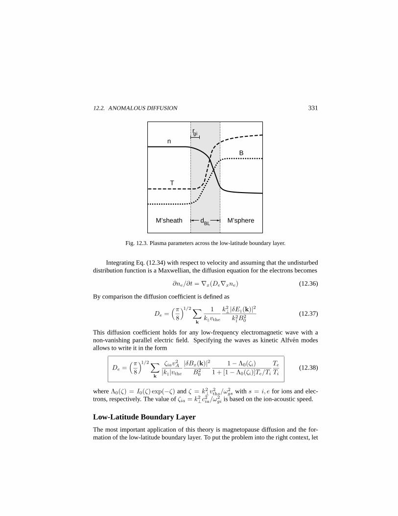
12.2. ANOMALOUS DIFFUSION 331
dBL
n
T
B
rgi
M’sheath M’sphere
Fig. 12.3. Plasma parameters across the low-latitude boundary layer.
Integrating Eq. (12.34) with respect to velocity and assuming that the undisturbeddistribution function is a Maxwellian, the diffusion equation for the electrons becomes
∂ne/∂t = ∇x(De∇xne) (12.36)
By comparison the diffusion coefficient is defined as
De =(π
8
)1/2 ∑
k
1k‖vthe
k2⊥|δE‖(k)|2
k2‖B
20
(12.37)
This diffusion coefficient holds for any low-frequency electromagnetic wave with anon-vanishing parallel electric field. Specifying the waves as kinetic Alfven modesallows to write it in the form
De =(π
8
)1/2 ∑
k
ζiav2A
|k‖|vthe
|δBx(k)|2B2
0
1− Λ0(ζi)1 + [1− Λ0(ζi)]Te/Ti
Te
Ti(12.38)
whereΛ0(ζ) = I0(ζ) exp(−ζ) andζ = k2⊥v2
ths/ω2gs with s = i, e for ions and elec-
trons, respectively. The value ofζia = k2⊥c2
ia/ω2gi is based on the ion-acoustic speed.
Low-Latitude Boundary Layer
The most important application of this theory is magnetopause diffusion and the for-mation of the low-latitude boundary layer. To put the problem into the right context, let

332 12. COLLECTIVE EFFECTS
10−2 100 102 104 10−16
10−12
10−8
10−4
100
Frequency in Hz
Spe
ctra
l Den
sity
in
V2 /m
2H
z
Fig. 12.4. Typical boundary layer electric wave spectrum.
us recall the physical conditions at the magnetopause. Figure 12.3 shows a schematiccollection of the variation of magnetic field, density, and temperature during a transitionfrom the magnetosheath across the low-latitude boundary layer of thicknessdBL intothe magnetosphere. For northward interplanetary magnetic field, the magnetopause isa non-permeable sharp discontinuity between the turbulent magnetosheath plasma andthe magnetosphere. The width of the boundary transition layer should be of the orderof the ion gyroradius, roughly 100 km. But observations demonstrate that the averagewidth of the transition is 1000–1200 km.
Estimates of the diffusion required for maintenance of such a thick boundary layershow that it must reach the Bohm limit, which at the magnetopause is of the orderof DB ≈ 109 m2/s, a comparably large value. It is hardly possible to reproduce thisvalue with any of the anomalous collision frequencies except for the lower-hybrid driftanomalous collision frequency. In order to compare with measured wave intensities itis convenient to use
Ww =(
1 +ω2
ω2ge
)(1 +
k2v2thi
ω2lh
)WE (12.39)
Usingγmax ≈ 0.3(vde/vthi)2ωlh, the collision frequency can be expressed as
νan,lh ≈ ωlh
(π
8
)1/2 mi
me
(1 +
ω2pe
ω2ge
)WE
nkBTi(12.40)
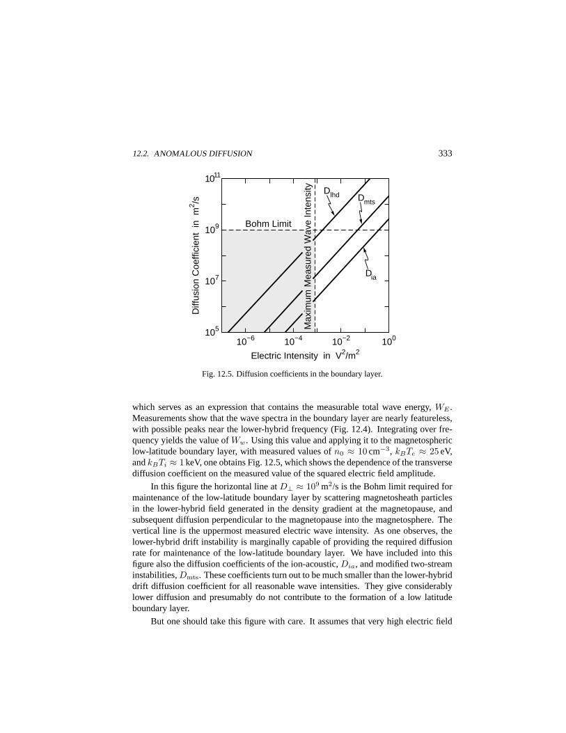
12.2. ANOMALOUS DIFFUSION 333
10−6 10−4 10−2 100
Electric Intensity in V2/m2
105
107
109
1011
Diff
usio
n C
oeffi
cien
t in
m2 /s
Dlhd Dmts
Dia
Bohm Limit
Max
imum
Mea
sure
d W
ave
Inte
nsity
Fig. 12.5. Diffusion coefficients in the boundary layer.
which serves as an expression that contains the measurable total wave energy,WE .Measurements show that the wave spectra in the boundary layer are nearly featureless,with possible peaks near the lower-hybrid frequency (Fig. 12.4). Integrating over fre-quency yields the value ofWw. Using this value and applying it to the magnetosphericlow-latitude boundary layer, with measured values ofn0 ≈ 10 cm−3, kBTe ≈ 25 eV,andkBTi ≈ 1 keV, one obtains Fig. 12.5, which shows the dependence of the transversediffusion coefficient on the measured value of the squared electric field amplitude.
In this figure the horizontal line atD⊥ ≈ 109 m2/s is the Bohm limit required formaintenance of the low-latitude boundary layer by scattering magnetosheath particlesin the lower-hybrid field generated in the density gradient at the magnetopause, andsubsequent diffusion perpendicular to the magnetopause into the magnetosphere. Thevertical line is the uppermost measured electric wave intensity. As one observes, thelower-hybrid drift instability is marginally capable of providing the required diffusionrate for maintenance of the low-latitude boundary layer. We have included into thisfigure also the diffusion coefficients of the ion-acoustic,Dia, and modified two-streaminstabilities,Dmts. These coefficients turn out to be much smaller than the lower-hybriddrift diffusion coefficient for all reasonable wave intensities. They give considerablylower diffusion and presumably do not contribute to the formation of a low latitudeboundary layer.
But one should take this figure with care. It assumes that very high electric field
334 12. COLLECTIVE EFFECTS
strengths can be reached. It is not established so far that such wave fields are realistic.Measurements do not sufficiently resolve the wave structures in space or time. In localgradients, however, where the gradient scale may even be near the electron gyroradius,wave intensities may be high enough to make lower-hybrid drift waves an efficientdiffusion mechanism. During disturbed times one would expect that reconnection willcause formation of the low-latitude boundary layer and yield plasma transport into themagnetosphere. In this case the anomalous lower-hybrid drift collisions provide thediffusivity which the successful models of reconnection are looking for.
12.3. Collisionless Shock Waves
One of the most important aspects of nonlinear plasma theory are collisionless shockwaves. Collisionless shocks exist both in laboratory and space plasma physics. Theproblem is to explain what causes the dissipation needed to generate the shock frontand to provide the irreversibility and entropy increase during the transition. When dis-cussing magnetohydrodynamic discontinuities in Chap. 8 of our companion book, itwas assumed that these dissipative processes are restricted to the narrow shock fronttransition layer. Hence, anomalous transport coefficients must be generated thereinby some instability mechanism. Most probable are ion-acoustic anomalous collisions,electron-acoustic anomalous collisions, though these are known to be low, Bunemananomalous collisions, though these can act only temporarily, and lower-hybrid driftanomalous collision, which need low plasmaβ. Related to the latter are modified two-stream anomalous collisions, which survive in high-β plasmas but have lower collisionfrequencies.
Because of the irreversibility of the shock transition process, a shock wave can-not be described as a purely steepened nonlinear wave. While wave steepening is atransitory process which, when not stopped, inevitably leads to wave breaking, shockwaves are stationary states with the breaking prevented by some other process, in gen-eral by dissipation. Any fast, slow, or intermediate shock is, from a macroscopic pointof view, a steepened fast, slow, or intermediate magnetosonic wave, with breaking in-hibited due to the balance of steepening and dissipation. Hence, nonlinear wave theoryis applicable to the shock process. The steepening of a fast magnetosonic wave is theignitor of the follow-up microscopic processes, which provide the dissipation insidethe shock front and cause irreversibility. In principle, such a picture will be correct forsufficiently slow shocks, where the flow speed leaves sufficient time for the steepeningand the subsequent evolution of the microscopic processes.
Low Mach number shocks will follow this scenario. But in high Mach numbershocks there will be not enough time for the anomalous process to provide the requiredcollision frequencies. When a critical Mach number is surpassed, new effects like par-ticle reflection from the shock front arise. Such shocks are called supercritical. In
12.3. COLLISIONLESS SHOCK WAVES 335
addition, the shock character depends strongly on the magnetic field direction. Quasi-perpendicular shocks behave more regularly than quasi-parallel shocks.
Rankine-Hugoniot Conditions
The Rankine-Hugoniot conditions do neither provide any information about the forma-tion of shocks nor about the intrinsic dissipative processes which are at work in theshock transition layer. Moreover, they are based on the one-fluid model of the plasma,which is a very rough approximation to reality. Therefore, they hold only sufficientlyfar away from the shock front itself, deep in the ideal magnetohydrodynamic regions toboth sides of the shock front. Prescribing the inflow parameters the serve as conditionsfrom which the outflow parameters can be calculated.
Denoting the upstream and downstream values by the indices 1 and 2, and defin-ing the following new variablesN = n2/n1, un = vn2/vn1, ut2 = vt2/vn1, uth1 =vth1/vn1, uth2 = vth2/vn1, bt1 = Bt1/(µ0min1v
2n1)
1/2, bt2 = Bt2/(µ0min1v2n1)
1/2,andbn = Bn/(µ0min1v
2n1)
1/2, the whole set of the shock jump conditions with non-vanishing flow across the shock may be written as
Nun = 12N(u2
th2 + u2n) + b2
t2 = 2(u2th1 + 1) + b2
t1
unbt2 − ut2bn = bt1 (12.41)
bt2bn − ut2 = bt1bn
5u2th2 + u2
n + u2t2 + 2bt2bt1 = 5u2
th1 + 1 + 2b2t1
From the third and fourth equation one finds for the tangential magnetic and velocityfields behind the shock
bt2 = bt1(1− b2n)/(un − b2
n)ut2 = bt1bn(1− un)/(un − b2
n)(12.42)
The rest of the equations can be reduced to a cubic equation for the normal velocity,un,behind the shock. But it is more interesting at this stage to consider the limiting caseof a perpendicular shock. This case is defined asbn = ut2 = 0, bt1 6= 0. The cubicequation becomes quadratic in this case
u2n −
(14 + 5
4u2th1 + 5
8b2t1
)un − 1
8b2t1 = 0 (12.43)
This equation yields the values of the quantities behind the shock in terms of those infront of the shock. In particular, the density, velocity and magnetic field jumps are all
336 12. COLLECTIVE EFFECTS
given by the same expression
1N
= un =(
bt2
bt1
)−1
=18
1 + 5u2
th1 + b2t1 +
[(1 + 5u2
th1 + 52b2
t1
)2+ 8b2
t1
]1/2
(12.44)and the jump in the temperature or the thermal velocity follows as
u2th2 = u2
th1 + 15 [1− u2
n + 2b2t1(1− u−1
n )] (12.45)
For the shock to exist one requires that the medium behind the shock is slowed down,and thereforeun < 1. This condition leads to the additional condition on the magne-tosonic Mach number of the incident flow
M =(
53u2
th1 + b2t1
)−1/2> 1 (12.46)
The last condition simply means that the flow is super-magnetosonic for fast perpen-dicular shocks to develop.
The jump conditions of the perpendicular shock given in Eq. (12.44) depend onthe upstream ratio of thermal-to-magnetic field energy density, i.e., on the plasma betaparameter in the upstream flow,β1. Forβ1 ¿ 1 the influence of the magnetic field isstrong. In this case the Mach number becomes the upstream Alfvenic Mach number,MA = vn1/vA1. In the opposite case, it is negligible, and the magnetohydrodynamicshock resembles a simple hydrodynamic shock. But one should be careful with thisconclusion, since the magnetohydrodynamic approximation readily fails in reality, andparticle and wave processes may become extremely important in shock dynamics.
The most important conclusion drawn from the above jump conditions is that forrelatively high Mach numbersM À 1 the jumps simplify to some expressions whichcan easily be used for estimating the strongest possible changes of the field quantitiesacross the shock transition in perpendicular shocks. For the original unormalized quan-tities these are written as
n1/n2 = Bt1/Bt2 = vn2/vn1 ≈ 1/4kBT2/mi ≈ 3v2
n1/16(12.47)
These conditions show that the density and magnetic fields in a perpendicular shock willnot increase by more than a factor of 4.
Theoretically, parallel shocks should behave like ordinary gasdynamic shocks, be-cause the magnetic field inside the shock is aligned exactly along the inflow and theshock normal, and thus drops out of the magnetohydrodynamic Rankine-Hugoniot con-ditions. But, again, one must be careful in drawing such a conclusion, since for fast
12.3. COLLISIONLESS SHOCK WAVES 337
shocks with strong magnetic fields,β1 < 1, the fast magnetosonic velocity parallel tothe field becomes the shear Alfven velocity, and the fast wave couples over to the shearAlfv en wave, which has a transverse magnetic field component. At the shock front themagnetosonic wave steepens, and this perpendicular field component increases. Hence,strictly parallel shock waves do not exist in a plasma. Near the shock front these shockscontain a transverse magnetic field component, and the shock wave becomes necessar-ily oblique and exhibits a complicated magnetic structure.
Critical Mach Numbers
The limit of extremely high Mach numbers given above is unrealistic. When the Machnumber of a collisionless shock becomes too large, the character of the shock transi-tion changes from laminar to turbulent. This change has to do with the process whichdissipates the inflowing kinetic and magnetic energies in order to increase the entropyduring shock transition and to generate irreversibility.
Laminar shock waves are steepened magnetohydrodynamic waves with breakingof the wave inhibited by dissipative effects. Two kinds of such dissipative effects maywork in laminar shock fronts. The first is Joule heating due to the generation of anoma-lous collisions and resistivities in the current layer inside the shock, the second is vis-cous interaction in the shock front. Both processes are mutually related. In wave steep-ening both processes account for the production of different flow, density, and potentiallevels on both sides of the shock front. Therefore, neglecting dissipation and consid-ering a solitary wave state should give an estimate of the maximum possible Machnumber in laminar shocks.
Figure 12.6 shows a soliton-shock configuration withB1 the undisturbed upstreamtangential magnetic field,Bm the soliton, andBs the shock amplitude. Consider theone-dimensional two-fluid model of magnetosonic waves at a perpendicular shock withthe magnetic field parallel to the front
d(nvsx)/dx = 0dBz/dx = µ0envey
mevixdvix/dx = eEx + eviyBz (12.48)
mevixdviy/dx = eEy − evixBz
mevixdviz/dx = 0
which is to be completed by the condition for the continuity of the tangential electricfield, dEy/dx = 0, and quasineutrality,ne ≈ ni. The x direction is normal to theshock front,z andy are tangential. The first of these equations is the continuity equa-tion, which holds for electrons and ions. The second equation is Ampere’s law withthe current carried exclusively by the electrons,jy = −envey. The three remainingequations are the equations of motion of the ions.

338 12. COLLECTIVE EFFECTS
Bz
Bm
Bs
B1
x
Shock
Soliton
Fig. 12.6. Magnetosonic soliton-shock model to estimateMcr.
The continuity equation implies constancy of the flux for both plasma componentssuch thatn = n1v1/vsx, where the index 1 refers to the values far upstream of theshock atx = −∞. There the electron and ion densities and speeds are the same. Hence,for the assumed quasineutrality the ion and electron perpendicular speeds are approx-imately the same at the shock as well,vix ≈ vex = vn. It follows thatEy = v1B1,n = n1v1/vn, and isEx = −Bzvey. This equation results from neglecting the verysmall contribution of the ions to they component of the velocity or from the fact thatonly the electrons are frozen-in. Remember that we consider perpendicular shocks withthe magnetic field only in thez direction and changing in value only across the shocktransition. In addition, summing the species in the equation forBz and integrating onceproduces for the normal component of the velocity
vn = vix = vex = v1 − (B2z −B2
1)/2µ0min1v1 (12.49)
which shows that the normal fluid velocity decreases in the shock. This form can beused to express the current speed
vey =1
µ0en1
dBz
dx
(1− B2
z −B21
2µ0min1v21
)(12.50)
With the help of these expressions one derives an equation for the magnetic field com-ponent tangential to the shock,Bz, which can be integrated once with respect tox inorder to be written in the form of the energy conservation of a pseudo-particle
(dBz/dx)2 = −2S(Bz) (12.51)
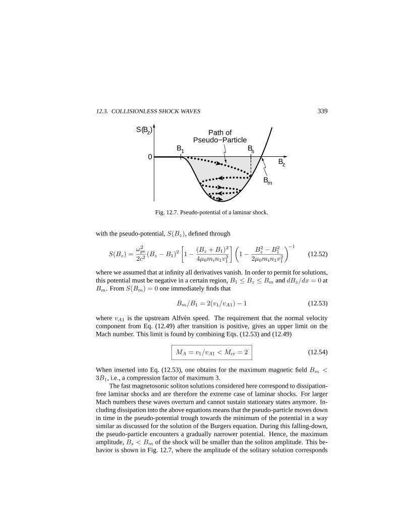
12.3. COLLISIONLESS SHOCK WAVES 339
S(Bz)
0 B1 Bs
Bz
Bm
Path of Pseudo−Particle
Fig. 12.7. Pseudo-potential of a laminar shock.
with the pseudo-potential,S(Bz), defined through
S(Bz) =ω2
pe
2c2(Bz −B1)2
[1− (Bz + B1)2
4µ0min1v21
](1− B2
z −B21
2µ0min1v21
)−1
(12.52)
where we assumed that at infinity all derivatives vanish. In order to permit for solutions,this potential must be negative in a certain region,B1 ≤ Bz ≤ Bm anddBz/dx = 0 atBm. FromS(Bm) = 0 one immediately finds that
Bm/B1 = 2(v1/vA1)− 1 (12.53)
wherevA1 is the upstream Alfven speed. The requirement that the normal velocitycomponent from Eq. (12.49) after transition is positive, gives an upper limit on theMach number. This limit is found by combining Eqs. (12.53) and (12.49)
MA = v1/vA1 < Mcr = 2 (12.54)
When inserted into Eq. (12.53), one obtains for the maximum magnetic fieldBm <3B1, i.e., a compression factor of maximum 3.
The fast magnetosonic soliton solutions considered here correspond to dissipation-free laminar shocks and are therefore the extreme case of laminar shocks. For largerMach numbers these waves overturn and cannot sustain stationary states anymore. In-cluding dissipation into the above equations means that the pseudo-particle moves downin time in the pseudo-potential trough towards the minimum of the potential in a waysimilar as discussed for the solution of the Burgers equation. During this falling-down,the pseudo-particle encounters a gradually narrower potential. Hence, the maximumamplitude,Bs < Bm of the shock will be smaller than the soliton amplitude. This be-havior is shown in Fig. 12.7, where the amplitude of the solitary solution corresponds

340 12. COLLECTIVE EFFECTS
to the zero-point of the pseudo-potential,Bm, with the shock amplitude being the firstdownward oscillation,Bs, in the potential.
Let us define the ratio of the maximum shock to the maximum soliton amplitude,Bs/Bm = α ≤ 1. Requiring thatvn > 0 and repeating the same calculation as before,we have approximately
Mcr ≈ 2α/(2α− 1) α > 1/2 (12.55)
for a resistive shock wave to exist in fast flows. For instance, forα = 0.9 one obtainsMcr = 2.25.
However, an absolute upper limit on the possible Mach number for resistive shocksis obtained from the simple argument that the downstream flow velocity,vn = vn2,should be less than the relevant downstream wave speed for information transport be-tween the obstacle and the shock. If this condition is not satisfied, the information aboutthe obstacle cannot reach the shock in a flow time, resistivity cannot sustain the shock,and resistive shocks cannot evolve. The condition imposed is related to theevolution-ary conditionof the shock. For fast shocks the wave speed for information transportfrom the obstacle to the shock is the fast mode velocity given in Eq. (I.9.100) of ourcompanion book. Heating of the plasma in the shock and behind increases the soundspeed. It is thus sufficient to require that the downstream flow speed should be less thanthe downstream sound speed,vn2 < cia2.
Evaluating this condition, by using the temperature jump and velocity drop acrossa perpendicular shock, it can be shown that the critical dissipative Mach number up towhich shocks can resistively be sustained is about
Mcr1 ≈ 2.7 (12.56)
This limit is valid for strictly perpendicular shocks with a magnetic field to shock nor-mal angleθBn = 90. For oblique shocks with smaller angles, the critical Mach num-ber decreases, and the shock becomes supercritical already at moderate Mach numbers.Enhancing the resistivity will cause the shock transition to widen. But resistivity cannotprevent supercritical shocks to break and to become turbulent. The most common andmost efficient way is the generation of shock feet and foreshock.
The critical Mach number,Mcr1, is only approximate and is obtained on the as-sumption that resistivity is the basic dissipation mechanism. A second, slightly largercritical Mach number,Mcr2, can be defined if anomalous viscosity is added. Anoma-lous viscosity heats the ions, increasing their momentum when passing through theshock. Accordingly, the second critical Mach number is defined as the Mach numberat which the downstream speed equals the downstream heated ion thermal velocity,vn = vthi2. Mcr2 depends on the downstream electron-to-ion temperature ratio, theincident plasma beta,β1, and the angleθBn1. It can be several times the first critical
12.4. SHOCK WAVE STRUCTURE 341
Mach number. BelowMcr2 the shock is sustained by resistivity and viscosity. AboveMcr2 it can only be supported by ion reflection into the upstream region as the basicdissipation mechanism.
But for extremely strong shocks with very high Mach numbers even ion reflectioncannot support the shock anymore, and a third critical Mach number will exist, becauseeven a very fast flow into the shock cannot reflect more ions than a certain percentageof the incident ions. Suchsuper-supercriticalshocks will heat the plasma to such hightemperatures that the magnetic field can be neglected and the shock will become gas-dynamic. Actually, compression of the magnetic field is restricted. Hence, the plasmamay indeed become super-heated. The third critical Mach number,Mcr3, would bethe solution of the balance equation between the downstream flow and sound speeds,vn = cs, wherecs is to be calculated by accounting for the unknown ion dynamics,reflection, and heating processes.
12.4. Shock Wave Structure
Collisionless shocks have a well-defined substructure, which depends on the angle be-tween the upstream magnetic field and the shock normal (see Sec. 8.5 of the companionvolume). For a given upstream magnetic field structure, this angle often depends onthe form and nature of the obstacle. For obstacles of finite extension around which theincident matter can flow, it changes with location along the shock. Shocks can have atotally different character at different locations and may thus have different structure.
Shock Foot
Mach numbers exceeding one or more of the the critical Mach numbers are not unusualin space and astrophysical plasmas. The solar wind has variable Mach numbers in therange1.5 < M < 15, with the lower and upper bounds depending on the state of solaractivity. Clearly, even during times of high Mach numbers the Earth’s bow shock waveexists. Astrophysical shock waves may have Mach numbers up to several thousands.Such shocks aresupercriticalor evensuper-supercriticalin contrast to thesubcriticalshocks with low Mach numbers. How can such shocks be sustained and how do theymanage to generate the required dissipation?
Within the framework of the cold plasma theory used in the previous section, thewidth of the soliton transition is determined by the electron inertial length,c/ωpe. Thisassumption is unrealistic for a shock. Widening due to dissipation increases the widthto v1/νan, and one expects the transition to be of the order of the ion gyroradius inthe compressed magnetic field of the shock ramp. The main property of supercriticalshocks is that they need to reflect particles from the shock front into the undisturbedflow region upstream of the shock. For some part of the incident particle population,
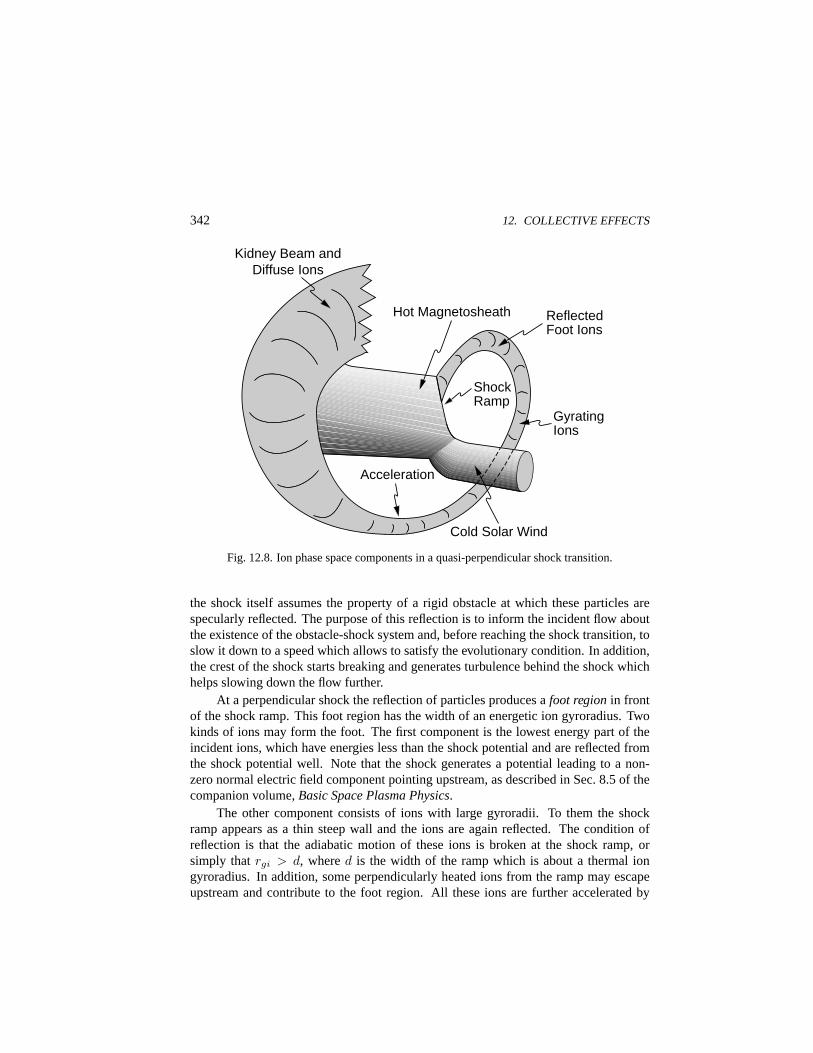
342 12. COLLECTIVE EFFECTS
Kidney Beam and Diffuse Ions
Reflected Foot Ions
Gyrating Ions
Shock Ramp
Hot Magnetosheath
Cold Solar Wind
Acceleration
Fig. 12.8. Ion phase space components in a quasi-perpendicular shock transition.
the shock itself assumes the property of a rigid obstacle at which these particles arespecularly reflected. The purpose of this reflection is to inform the incident flow aboutthe existence of the obstacle-shock system and, before reaching the shock transition, toslow it down to a speed which allows to satisfy the evolutionary condition. In addition,the crest of the shock starts breaking and generates turbulence behind the shock whichhelps slowing down the flow further.
At a perpendicular shock the reflection of particles produces afoot regionin frontof the shock ramp. This foot region has the width of an energetic ion gyroradius. Twokinds of ions may form the foot. The first component is the lowest energy part of theincident ions, which have energies less than the shock potential and are reflected fromthe shock potential well. Note that the shock generates a potential leading to a non-zero normal electric field component pointing upstream, as described in Sec. 8.5 of thecompanion volume,Basic Space Plasma Physics.
The other component consists of ions with large gyroradii. To them the shockramp appears as a thin steep wall and the ions are again reflected. The condition ofreflection is that the adiabatic motion of these ions is broken at the shock ramp, orsimply thatrgi > d, whered is the width of the ramp which is about a thermal iongyroradius. In addition, some perpendicularly heated ions from the ramp may escapeupstream and contribute to the foot region. All these ions are further accelerated by
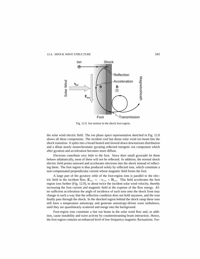
12.4. SHOCK WAVE STRUCTURE 343
B B
+ Ion Shock
Reflection
Transmission Foot
Sol
ar W
ind Acceleration
Magnetosheath
vsw
Esw
Fig. 12.9. Ion motion in the shock foot region.
the solar wind electric field. The ion phase space representation sketched in Fig. 12.8shows all these components. The incident cool but dense solar wind ion beam hits theshock transition. It splits into a broad heated and slowed-down downstream distributionand a dilute nearly monochromatic gyrating reflected energetic ion component whichafter gyration and acceleration becomes more diffuse.
Electrons contribute very little to the foot. Since their small gyroradii let thembehave adiabatically, most of them will not be reflected. In addition, the normal shockelectric field points sunward and accelerates electrons into the shock instead of reflect-ing them. The foot region is thus produced solely by reflected ions, which constitute anon-compensated perpendicular current whose magnetic field forms the foot.
A large part of the gyratory orbit of the foot-region ions is parallel to the elec-tric field in the incident flow,Esw = −vsw × Bsw. This field accelerates the footregion ions further (Fig. 12.9), to about twice the incident solar wind velocity, therebyincreasing the foot current and magnetic field at the expense of the flow energy. Af-ter sufficient acceleration the angle of incidence of such ions onto the shock front maychange in such a way that the reflection condition does not hold anymore, and the ionsfinally pass through the shock. In the shocked region behind the shock ramp these ionsstill have a temperature anisotropy and generate anisotropy-driven wave turbulence,until they are quasilinearly scattered and merge into the background.
Foot-region ions constitute a fast ion beam in the solar wind flow and, in addi-tion, cause instability and wave activity by counterstreaming beam interaction. Hence,the foot region contains an enhanced level of low-frequency magnetic fluctuations. Fur-
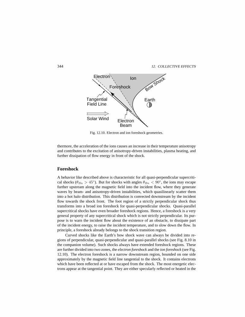
344 12. COLLECTIVE EFFECTS
Ion
Foreshock
Electron
Tangential Field Line
Solar Wind Electron Beam
Earth
Bow Shock
Fig. 12.10. Electron and ion foreshock geometries.
thermore, the acceleration of the ions causes an increase in their temperature anisotropyand contributes to the excitation of anisotropy-driven instabilities, plasma heating, andfurther dissipation of flow energy in front of the shock.
Foreshock
A behavior like described above is characteristic for all quasi-perpendicular supercriti-cal shocks (θBn > 45). But for shocks with anglesθBn < 90, the ions may escapefurther upstream along the magnetic field into the incident flow, where they generatewaves by beam- and anisotropy-driven instabilities, which quasilinearly scatter theminto a hot halo distribution. This distribution is convected downstream by the incidentflow towards the shock front. The foot region of a strictly perpendicular shock thustransforms into a broad ion foreshock for quasi-perpendicular shocks. Quasi-parallelsupercritical shocks have even broader foreshock regions. Hence, a foreshock is a verygeneral property of any supercritical shock which is not strictly perpendicular. Its pur-pose is to warn the incident flow about the existence of an obstacle, to dissipate partof the incident energy, to raise the incident temperature, and to slow down the flow. Inprinciple, a foreshock already belongs to the shock transition region.
Curved shocks like the Earth’s bow shock wave can always be divided into re-gions of perpendicular, quasi-perpendicular and quasi-parallel shocks (see Fig. 8.10 inthe companion volume). Such shocks always have extended foreshock regions. Theseare further divided into two zones, theelectron foreshockand theion foreshock(see Fig.12.10). The electron foreshock is a narrow downstream region, bounded on one sideapproximately by the magnetic field line tangential to the shock. It contains electronswhich have been reflected at or have escaped from the shock. The most energetic elec-trons appear at the tangential point. They are either specularly reflected or heated in the
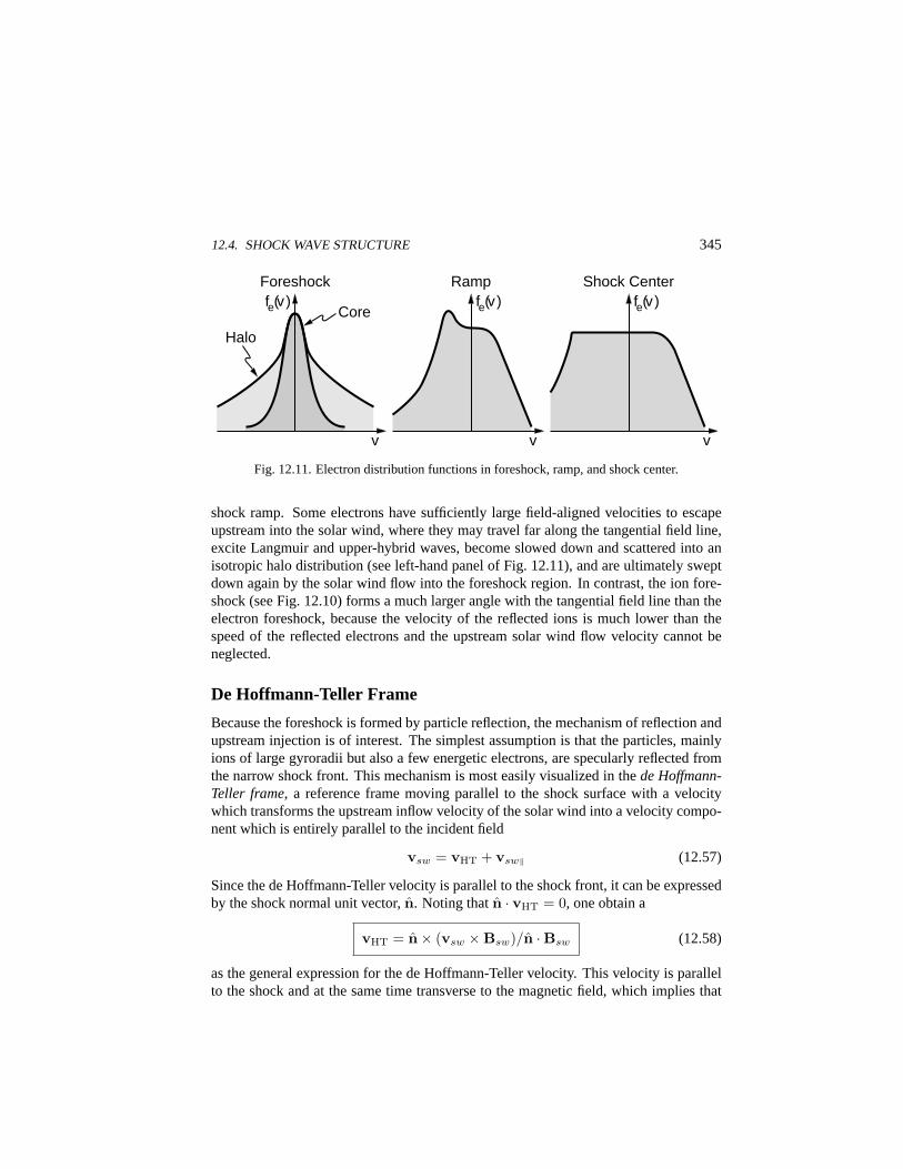
12.4. SHOCK WAVE STRUCTURE 345
v
fe(v ) Core
Halo
Foreshock
v
Ramp fe(v )
Shock Center fe(v )
v
Fig. 12.11. Electron distribution functions in foreshock, ramp, and shock center.
shock ramp. Some electrons have sufficiently large field-aligned velocities to escapeupstream into the solar wind, where they may travel far along the tangential field line,excite Langmuir and upper-hybrid waves, become slowed down and scattered into anisotropic halo distribution (see left-hand panel of Fig. 12.11), and are ultimately sweptdown again by the solar wind flow into the foreshock region. In contrast, the ion fore-shock (see Fig. 12.10) forms a much larger angle with the tangential field line than theelectron foreshock, because the velocity of the reflected ions is much lower than thespeed of the reflected electrons and the upstream solar wind flow velocity cannot beneglected.
De Hoffmann-Teller Frame
Because the foreshock is formed by particle reflection, the mechanism of reflection andupstream injection is of interest. The simplest assumption is that the particles, mainlyions of large gyroradii but also a few energetic electrons, are specularly reflected fromthe narrow shock front. This mechanism is most easily visualized in thede Hoffmann-Teller frame, a reference frame moving parallel to the shock surface with a velocitywhich transforms the upstream inflow velocity of the solar wind into a velocity compo-nent which is entirely parallel to the incident field
vsw = vHT + vsw‖ (12.57)
Since the de Hoffmann-Teller velocity is parallel to the shock front, it can be expressedby the shock normal unit vector,n. Noting thatn · vHT = 0, one obtain a
vHT = n× (vsw ×Bsw)/n ·Bsw (12.58)
as the general expression for the de Hoffmann-Teller velocity. This velocity is parallelto the shock and at the same time transverse to the magnetic field, which implies that
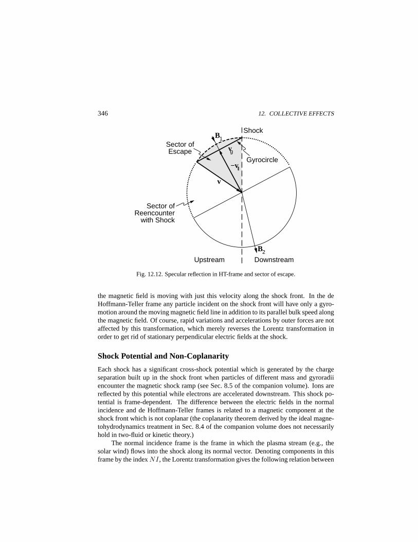
346 12. COLLECTIVE EFFECTS
B1
B2
Downstream Upstream
Sector of Reencounter
with Shock
Sector of Escape
Shock
Gyrocircle −v||
v
vg
Fig. 12.12. Specular reflection in HT-frame and sector of escape.
the magnetic field is moving with just this velocity along the shock front. In the deHoffmann-Teller frame any particle incident on the shock front will have only a gyro-motion around the moving magnetic field line in addition to its parallel bulk speed alongthe magnetic field. Of course, rapid variations and accelerations by outer forces are notaffected by this transformation, which merely reverses the Lorentz transformation inorder to get rid of stationary perpendicular electric fields at the shock.
Shock Potential and Non-Coplanarity
Each shock has a significant cross-shock potential which is generated by the chargeseparation built up in the shock front when particles of different mass and gyroradiiencounter the magnetic shock ramp (see Sec. 8.5 of the companion volume). Ions arereflected by this potential while electrons are accelerated downstream. This shock po-tential is frame-dependent. The difference between the electric fields in the normalincidence and de Hoffmann-Teller frames is related to a magnetic component at theshock front which is not coplanar (the coplanarity theorem derived by the ideal magne-tohydrodynamics treatment in Sec. 8.4 of the companion volume does not necessarilyhold in two-fluid or kinetic theory.)
The normal incidence frame is the frame in which the plasma stream (e.g., thesolar wind) flows into the shock along its normal vector. Denoting components in thisframe by the indexNI, the Lorentz transformation gives the following relation between
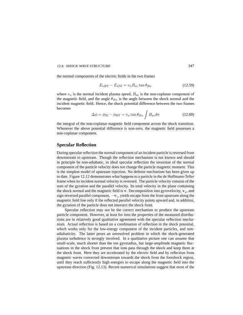
12.4. SHOCK WAVE STRUCTURE 347
the normal components of the electric fields in the two frames
EnHT − EnNI = vnBnc tan θBn (12.59)
wherevn is the normal incident plasma speed,Bnc is the non-coplanar component ofthe magnetic field, and the angleθBn is the angle between the shock normal and theincident magnetic field. Hence, the shock potential difference between the two framesbecomes
∆φ = φNI − φHT = vn tan θBn
∫Bncdn (12.60)
the integral of the non-coplanar magnetic field component across the shock transition.Whenever the above potential difference is non-zero, the magnetic field possesses anon-coplanar component.
Specular Reflection
During specular reflection the normal component of an incident particle is reversed fromdownstream to upstream. Though the reflection mechanism is not known and shouldin principle be non-adiabatic, in ideal specular reflection the inversion of the normalcomponent of the particle velocity does not change the particle magnetic moment. Thisis the simplest model of upstream injection. No definite mechanism has been given upto date. Figure 12.12 demonstrates what happens to a particle in the de Hoffmann-Tellerframe when its incident normal velocity is reversed. The particle velocity consists of thesum of the gyration and the parallel velocity. Its total velocity in the plane containingthe shock normal and the magnetic field isv. Decomposition into gyrovelocity,vg, andsign-reversed parallel component,−v‖, yields escape from the front upstream along themagnetic field line only if the reflected parallel velocity points upward and, in addition,the gyration of the particle does not intersect the shock front.
Specular reflection may not be the correct mechanism to produce the upstreamparticle component. However, at least for ions the properties of the measured distribu-tions are in relatively good qualitative agreement with the specular reflection mecha-nism. Actual reflection is based on a combination of reflection in the shock potential,which works only for the low-energy component of the incident particles, and non-adiabaticity. The latter poses an unresolved problem in which the shock-generatedplasma turbulence is strongly involved. In a qualitative picture one can assume thatsmall-scale, much shorter than the ion gyroradius, but large-amplitude magnetic fluc-tuations in the shock front prevent that ions pass through the shock and keep them atthe shock front. Here they are accelerated by the electric field and by reflection frommagnetic waves convected downstream towards the shock from the foreshock region,until they reach sufficiently high energies to escape along the magnetic field into theupstream direction (Fig. 12.13). Recent numerical simulations suggest that most of the

348 12. COLLECTIVE EFFECTS
Sho
ck
B
Escaping Ion
B Incident Ion Path
Upstream
Trapped
Downstream
Fig. 12.13. Trapping and acceleration of ion in shock ramp.
specularly reflected ions are captured in the shock reformation process by the newlyformed shock and find themselves soon after reflection behind the shock ramp in thedownstream region. The upstream escaping particle component is thus composed justof the shock confined ions which are at rest in the de Hoffmann-Teller frame until theybecome energized sufficiently much and may escape from the shock.
Populating the foreshock region, these ion beams excite a high level of wave inten-sity, which scatters the ions self-consistently into so-calledkidney beamdistributions.Further down in the foreshock the ion distributions evolve into a nearly isotropicringdistribution. This ring distribution is taken up by the solar wind in the foreshock andflows in the direction of the shock. Figure 12.14 shows the evolution of a reflectedion beam in the foreshock into a kidney and a ring around the solar wind beam, whenpassing from the boundary of the foreshock into the heart of the foreshock.
Upstream Waves and Shock Reformation
The reflected ion beams in the foreshock region are a source of free energy and driveseveral ion-ion beam instabilities. The two beams involved in the interaction are thedense but cold incident solar wind and the warm reflected ion beam, which is only alittle less dense than the solar wind. The dominant ion beam instability in the fore-shock is the right-hand resonant instability (see Fig. 5.10). The mode is an Alfven-cyclotron mode, which scatters the ion beam into the diffuse ion distribution of thedeeper foreshock. Part of this diffuse distribution may reach high energies due to addi-
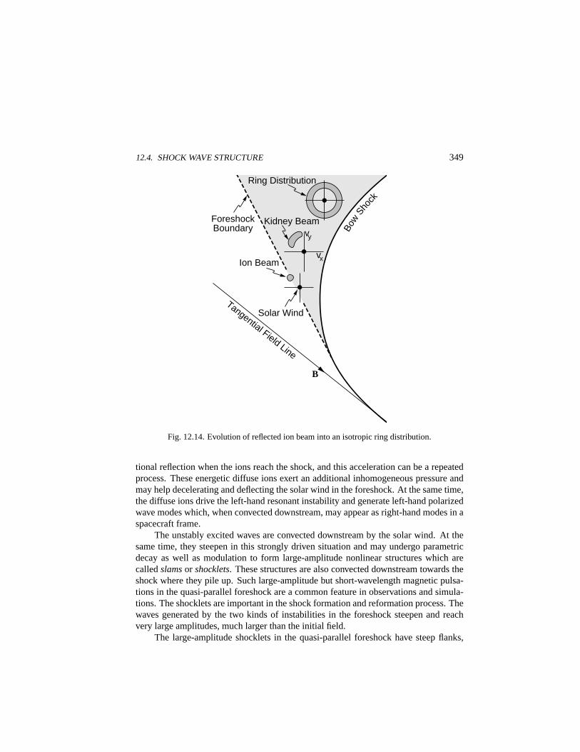
12.4. SHOCK WAVE STRUCTURE 349
Bow
Shock
Ring Distribution
Foreshock Boundary
Ion Beam
Solar Wind
B
vy
vx
Tangential Field Line
Kidney Beam
Fig. 12.14. Evolution of reflected ion beam into an isotropic ring distribution.
tional reflection when the ions reach the shock, and this acceleration can be a repeatedprocess. These energetic diffuse ions exert an additional inhomogeneous pressure andmay help decelerating and deflecting the solar wind in the foreshock. At the same time,the diffuse ions drive the left-hand resonant instability and generate left-hand polarizedwave modes which, when convected downstream, may appear as right-hand modes in aspacecraft frame.
The unstably excited waves are convected downstream by the solar wind. At thesame time, they steepen in this strongly driven situation and may undergo parametricdecay as well as modulation to form large-amplitude nonlinear structures which arecalledslamsor shocklets. These structures are also convected downstream towards theshock where they pile up. Such large-amplitude but short-wavelength magnetic pulsa-tions in the quasi-parallel foreshock are a common feature in observations and simula-tions. The shocklets are important in the shock formation and reformation process. Thewaves generated by the two kinds of instabilities in the foreshock steepen and reachvery large amplitudes, much larger than the initial field.
The large-amplitude shocklets in the quasi-parallel foreshock have steep flanks,
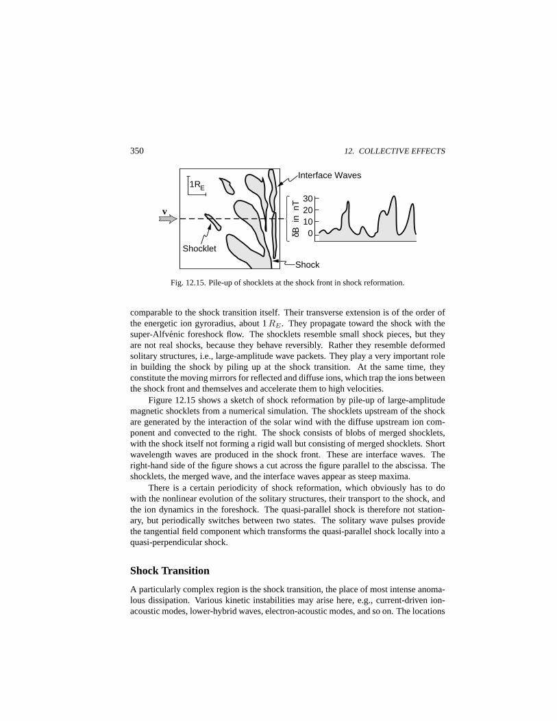
350 12. COLLECTIVE EFFECTS
Shock
Shocklet
Interface Waves
30 20 10 0
v
δB i
n n
T
1RE
Fig. 12.15. Pile-up of shocklets at the shock front in shock reformation.
comparable to the shock transition itself. Their transverse extension is of the order ofthe energetic ion gyroradius, about 1RE . They propagate toward the shock with thesuper-Alfvenic foreshock flow. The shocklets resemble small shock pieces, but theyare not real shocks, because they behave reversibly. Rather they resemble deformedsolitary structures, i.e., large-amplitude wave packets. They play a very important rolein building the shock by piling up at the shock transition. At the same time, theyconstitute the moving mirrors for reflected and diffuse ions, which trap the ions betweenthe shock front and themselves and accelerate them to high velocities.
Figure 12.15 shows a sketch of shock reformation by pile-up of large-amplitudemagnetic shocklets from a numerical simulation. The shocklets upstream of the shockare generated by the interaction of the solar wind with the diffuse upstream ion com-ponent and convected to the right. The shock consists of blobs of merged shocklets,with the shock itself not forming a rigid wall but consisting of merged shocklets. Shortwavelength waves are produced in the shock front. These are interface waves. Theright-hand side of the figure shows a cut across the figure parallel to the abscissa. Theshocklets, the merged wave, and the interface waves appear as steep maxima.
There is a certain periodicity of shock reformation, which obviously has to dowith the nonlinear evolution of the solitary structures, their transport to the shock, andthe ion dynamics in the foreshock. The quasi-parallel shock is therefore not station-ary, but periodically switches between two states. The solitary wave pulses providethe tangential field component which transforms the quasi-parallel shock locally into aquasi-perpendicular shock.
Shock Transition
A particularly complex region is the shock transition, the place of most intense anoma-lous dissipation. Various kinetic instabilities may arise here, e.g., current-driven ion-acoustic modes, lower-hybrid waves, electron-acoustic modes, and so on. The locations
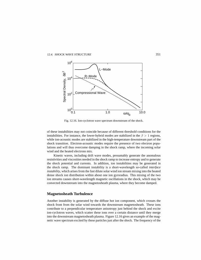
12.4. SHOCK WAVE STRUCTURE 351
L−Mode
R−Mode
Compressional Wave
100
102
104
106 S
pect
ral D
ensi
ty,
δB2
0.1 1.0 10.0 ω /ωgi
Fig. 12.16. Ion-cyclotron wave spectrum downstream of the shock.
of these instabilities may not coincide because of different threshold conditions for theinstabilities. For instance, the lower-hybrid modes are stabilized in theβ > 1 regions,while ion-acoustic modes are stabilized in the high-temperature downstream part of theshock transition. Electron-acoustic modes require the presence of two electron popu-lations and will thus overcome damping in the shock ramp, where the incoming solarwind and the heated electrons mix.
Kinetic waves, including drift wave modes, presumably generate the anomalousresistivities and viscosities needed in the shock ramp to increase entropy and to generatethe shock potential and currents. In addition, ion instabilities may be generated inthe shock ramp. The dominant instability is a short-wavelength so-calledinterfaceinstability, which arises from the fast dilute solar wind ion stream mixing into the heateddense shock ion distribution within about one ion gyroradius. This mixing of the twoion streams causes short-wavelength magnetic oscillations in the shock, which may beconvected downstream into the magnetosheath plasma, where they become damped.
Magnetosheath Turbulence
Another instability is generated by the diffuse hot ion component, which crosses theshock front from the solar wind towards the downstream magnetosheath. These ionscontribute to a perpendicular temperature anisotropy just behind the shock and exciteion-cyclotron waves, which scatter these ions over a certain distance until they mergeinto the downstream magnetosheath plasma. Figure 12.16 gives an example of the mag-netic wave spectrum excited by these particles just after the shock. The frequency of the
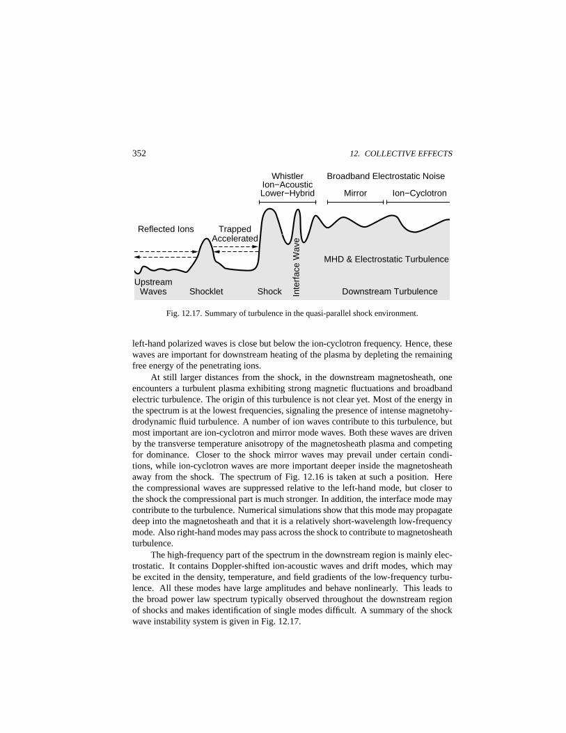
352 12. COLLECTIVE EFFECTS
Whistler Ion−Acoustic Lower−Hybrid
Broadband Electrostatic Noise
Mirror Ion−Cyclotron
Trapped Accelerated
Reflected Ions
Upstream Waves Shocklet Shock In
terf
ace
Wav
e Downstream Turbulence
MHD & Electrostatic Turbulence
Fig. 12.17. Summary of turbulence in the quasi-parallel shock environment.
left-hand polarized waves is close but below the ion-cyclotron frequency. Hence, thesewaves are important for downstream heating of the plasma by depleting the remainingfree energy of the penetrating ions.
At still larger distances from the shock, in the downstream magnetosheath, oneencounters a turbulent plasma exhibiting strong magnetic fluctuations and broadbandelectric turbulence. The origin of this turbulence is not clear yet. Most of the energy inthe spectrum is at the lowest frequencies, signaling the presence of intense magnetohy-drodynamic fluid turbulence. A number of ion waves contribute to this turbulence, butmost important are ion-cyclotron and mirror mode waves. Both these waves are drivenby the transverse temperature anisotropy of the magnetosheath plasma and competingfor dominance. Closer to the shock mirror waves may prevail under certain condi-tions, while ion-cyclotron waves are more important deeper inside the magnetosheathaway from the shock. The spectrum of Fig. 12.16 is taken at such a position. Herethe compressional waves are suppressed relative to the left-hand mode, but closer tothe shock the compressional part is much stronger. In addition, the interface mode maycontribute to the turbulence. Numerical simulations show that this mode may propagatedeep into the magnetosheath and that it is a relatively short-wavelength low-frequencymode. Also right-hand modes may pass across the shock to contribute to magnetosheathturbulence.
The high-frequency part of the spectrum in the downstream region is mainly elec-trostatic. It contains Doppler-shifted ion-acoustic waves and drift modes, which maybe excited in the density, temperature, and field gradients of the low-frequency turbu-lence. All these modes have large amplitudes and behave nonlinearly. This leads tothe broad power law spectrum typically observed throughout the downstream regionof shocks and makes identification of single modes difficult. A summary of the shockwave instability system is given in Fig. 12.17.
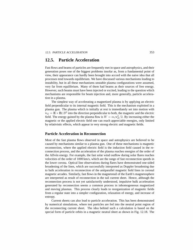
12.5. PARTICLE ACCELERATION 353
12.5. Particle Acceleration
Fast flows and beams of particles are frequently met in space and astrophysics, and theirgeneration poses one of the biggest problems insofar as, from a fundamental point ofview, their appearance can hardly been brought into accord with the naive idea that allprocesses tend towards equilibrium. We have discussed various mechanisms leading toinstability, but in all these mechanisms unstable plasma configurations were assumed,very far from equilibrium. Many of them had beams as their sources of free energy.However, such beams must have been injected or excited, leading to the question whichmechanisms are responsible for beam injection and, more generally, particle accelera-tion in a plasma.
The simplest way of accelerating a magnetized plasma is by applying an electricfield perpendicular to its internal magnetic field. This is the mechanism exploited in aplasma gun. The plasma which is initially at rest is immediately set into motion withvE = E×B/B2 into the direction perpendicular to both, the magnetic and the electricfield. The energy gained by the plasma flow isW = miv2
E/2. By increasing either themagnetic or the applied electric field one can reach appreciable energies, only limitedby relativistic effects, which appear in very strong electric and magnetic fields.
Particle Acceleration in Reconnection
Most of the fast plasma flows observed in space and astrophysics are believed to becaused by mechanisms similar to a plasma gun. One of these mechanisms is magneticreconnection, where the applied electric field is the induction field caused in the re-connection process, and the acceleration of the plasma reaches energies of the order ofthe Alfven energy. For example, the fast solar wind outflow during solar flares reachesvelocities of the order of 1000 km/s, which are the range of fast reconnection speeds inthe lower corona. Optical line observations during flares have demonstrated one-sidedbroadening of the lines, which are successfully interpreted as Doppler broadening dueto bulk acceleration in reconnection of the antiparallel magnetic field lines in coronalmagnetic arcades. Similarly, fast flows in the magnetotail of the Earth’s magnetosphereare interpreted as result of reconnection in the tail current sheet. Hence, although thereconnection process is not yet satisfactorily understood, impulsive bulk accelerationgenerated by reconnection seems a common process in inhomogeneous magnetizedand moving plasmas. This process clearly leads to reorganization of magnetic fieldsfrom a regular state into a simpler configuration, relaxation of energy, and increase ofentropy.
Current sheets can also lead to particle acceleration. This has been demonstratedby numerical simulations, where test particles are fed into the neutral point region ofthe reconnecting current sheet. The idea behind such a calculation is based on thespecial form of particle orbits in a magnetic neutral sheet as shown in Fig. 12.18. The
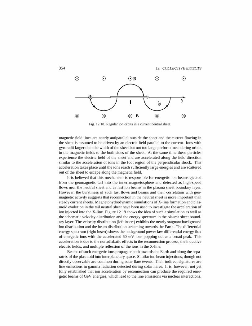
354 12. COLLECTIVE EFFECTS
B
−B
+ rgi j y
Fig. 12.18. Regular ion orbits in a current neutral sheet.
magnetic field lines are nearly antiparallel outside the sheet and the current flowing inthe sheet is assumed to be driven by an electric field parallel to the current. Ions withgyroradii larger than the width of the sheet but not too large perform meandering orbitsin the magnetic fields to the both sides of the sheet. At the same time these particlesexperience the electric field of the sheet and are accelerated along the field directionsimilar to the acceleration of ions in the foot region of the perpendicular shock. Thisacceleration takes place until the ions reach sufficiently large energies and are scatteredout of the sheet to escape along the magnetic field.
It is believed that this mechanism is responsible for energetic ion beams ejectedfrom the geomagnetic tail into the inner magnetosphere and detected as high-speedflows near the neutral sheet and as fast ion beams in the plasma sheet boundary layer.However, the burstiness of such fast flows and beams and their correlation with geo-magnetic activity suggests that reconnection in the neutral sheet is more important thansteady current sheets. Magnetohydrodynamic simulations of X-line formation and plas-moid evolution in the tail neutral sheet have been used to investigate the acceleration ofion injected into the X-line. Figure 12.19 shows the idea of such a simulation as well asthe schematic velocity distribution and the energy spectrum in the plasma sheet bound-ary layer. The velocity distribution (left insert) exhibits the nearly stagnant backgroundion distribution and the beam distribution streaming towards the Earth. The differentialenergy spectrum (right insert) shows the background power law differential energy fluxof energetic ions with the accelerated 60 keV ions popping out as a broad peak. Thisacceleration is due to the nonadiabatic effects in the reconnection process, the inductiveelectric fields, and multiple reflection of the ions in the X-line.
Beams of such energetic ions propagate both towards the Earth and along the sepa-ratrix of the plasmoid into interplanetary space. Similar ion beam injections, though notdirectly observable are common during solar flare events. Their indirect signatures areline emissions in gamma radiation detected during solar flares. It is, however, not yetfully established that ion acceleration by reconnection can produce the required ener-getic beams of GeV energies, which lead to the line emissions via nuclear interactions.
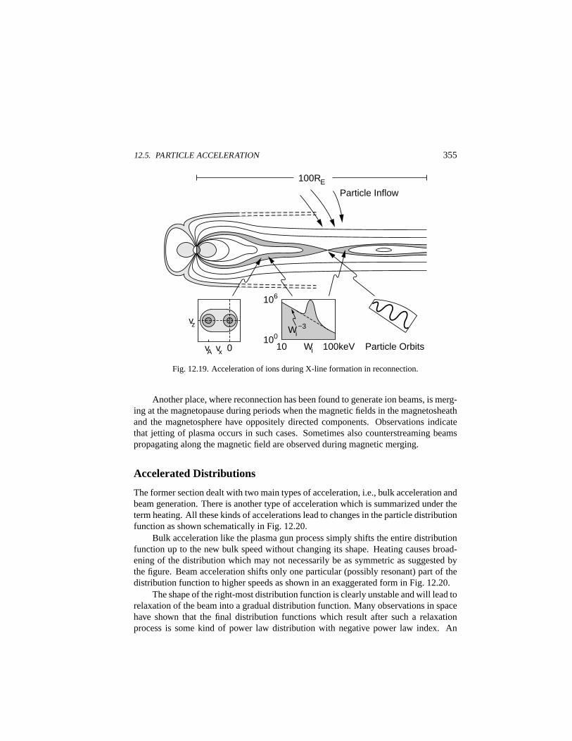
12.5. PARTICLE ACCELERATION 355
100RE
Particle Orbits
vz
vA 0 vx
106
100
10 100keV Wi
Wi−3
Particle Inflow
Fig. 12.19. Acceleration of ions during X-line formation in reconnection.
Another place, where reconnection has been found to generate ion beams, is merg-ing at the magnetopause during periods when the magnetic fields in the magnetosheathand the magnetosphere have oppositely directed components. Observations indicatethat jetting of plasma occurs in such cases. Sometimes also counterstreaming beamspropagating along the magnetic field are observed during magnetic merging.
Accelerated Distributions
The former section dealt with two main types of acceleration, i.e., bulk acceleration andbeam generation. There is another type of acceleration which is summarized under theterm heating. All these kinds of accelerations lead to changes in the particle distributionfunction as shown schematically in Fig. 12.20.
Bulk acceleration like the plasma gun process simply shifts the entire distributionfunction up to the new bulk speed without changing its shape. Heating causes broad-ening of the distribution which may not necessarily be as symmetric as suggested bythe figure. Beam acceleration shifts only one particular (possibly resonant) part of thedistribution function to higher speeds as shown in an exaggerated form in Fig. 12.20.
The shape of the right-most distribution function is clearly unstable and will lead torelaxation of the beam into a gradual distribution function. Many observations in spacehave shown that the final distribution functions which result after such a relaxationprocess is some kind of power law distribution with negative power law index. An
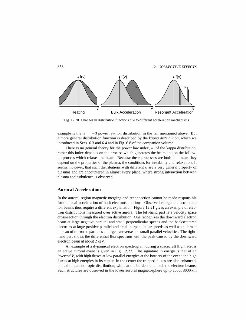
356 12. COLLECTIVE EFFECTS
f(v) f(v)
Heating Bulk Acceleration
f(v)
Resonant Acceleration v v v
Fig. 12.20. Changes in distribution functions due to different acceleration mechanisms.
example is theα = −3 power law ion distribution in the tail mentioned above. Buta more general distribution function is described by thekappa distribution, which weintroduced in Secs. 6.3 and 6.4 and in Fig. 6.8 of the companion volume.
There is no general theory for the power law index,κ, of the kappa distribution,rather this index depends on the process which generates the beam and on the follow-up process which relaxes the beam. Because these processes are both nonlinear, theydepend on the properties of the plasma, the conditions for instability and relaxation. Itseems, however, that such distributions with differentκ are a very general property ofplasmas and are encountered in almost every place, where strong interaction betweenplasma and turbulence is observed.
Auroral Acceleration
In the auroral region magnetic merging and reconnection cannot be made responsiblefor the local acceleration of both electrons and ions. Observed energetic electron andion beams thus require a different explanation. Figure 12.21 gives an example of elec-tron distributions measured over active aurora. The left-hand part is a velocity spacecross-section through the electron distribution. One recognizes the downward electronbeam at large negative parallel and small perpendicular speeds and the backscatteredelectrons at large positive parallel and small perpendicular speeds as well as the broadplateau of mirrored particles at large transverse and small parallel velocities. The right-hand part shows the differential flux spectrum with the peak caused by the downwardelectron beam at about 2 keV.
An example of a dynamical electron spectrogram during a spacecraft flight acrossan active auroral event is given in Fig. 12.22. The signature in energy is that of aninverted V, with high fluxes at low parallel energies at the borders of the event and highfluxes at high energies in its center. In the center the trapped fluxes are also enhanced,but exhibit an isotropic distribution, while at the borders one finds the electron beams.Such structures are observed in the lower auroral magnetosphere up to about 3000 km
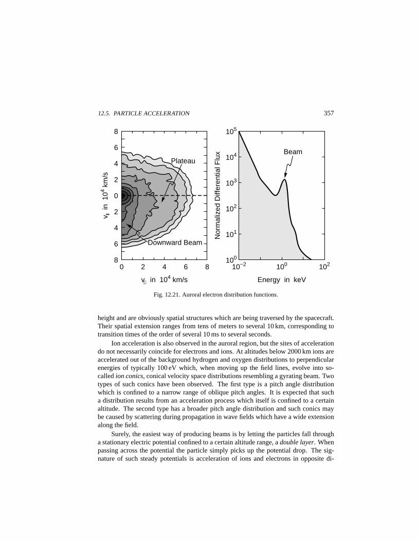
12.5. PARTICLE ACCELERATION 357
101
103
105
Beam
10−2 100 102
Energy in keV
Nor
mal
ized
Diff
eren
tial F
lux
0
v⊥ in 104 km/s
v ||
in 1
04 km
/s
Plateau
8 2 4 6 8
6
4
2
0
2
4
6
8
Downward Beam
100
102
104
Fig. 12.21. Auroral electron distribution functions.
height and are obviously spatial structures which are being traversed by the spacecraft.Their spatial extension ranges from tens of meters to several 10 km, corresponding totransition times of the order of several 10 ms to several seconds.
Ion acceleration is also observed in the auroral region, but the sites of accelerationdo not necessarily coincide for electrons and ions. At altitudes below 2000 km ions areaccelerated out of the background hydrogen and oxygen distributions to perpendicularenergies of typically 100 eV which, when moving up the field lines, evolve into so-calledion conics, conical velocity space distributions resembling a gyrating beam. Twotypes of such conics have been observed. The first type is a pitch angle distributionwhich is confined to a narrow range of oblique pitch angles. It is expected that sucha distribution results from an acceleration process which itself is confined to a certainaltitude. The second type has a broader pitch angle distribution and such conics maybe caused by scattering during propagation in wave fields which have a wide extensionalong the field.
Surely, the easiest way of producing beams is by letting the particles fall througha stationary electric potential confined to a certain altitude range, adouble layer. Whenpassing across the potential the particle simply picks up the potential drop. The sig-nature of such steady potentials is acceleration of ions and electrons in opposite di-
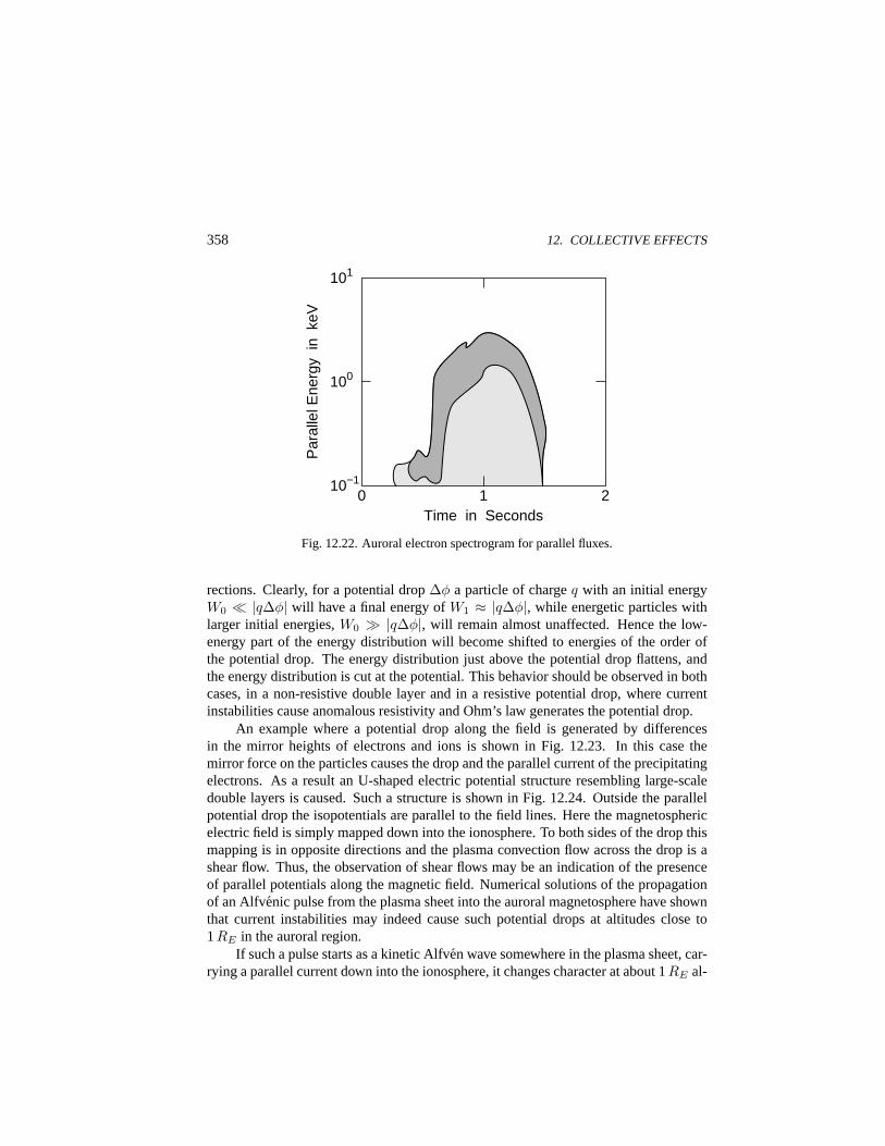
358 12. COLLECTIVE EFFECTS
0 10−1
100
101
Par
alle
l Ene
rgy
in k
eV
Time in Seconds 1 2
Fig. 12.22. Auroral electron spectrogram for parallel fluxes.
rections. Clearly, for a potential drop∆φ a particle of chargeq with an initial energyW0 ¿ |q∆φ| will have a final energy ofW1 ≈ |q∆φ|, while energetic particles withlarger initial energies,W0 À |q∆φ|, will remain almost unaffected. Hence the low-energy part of the energy distribution will become shifted to energies of the order ofthe potential drop. The energy distribution just above the potential drop flattens, andthe energy distribution is cut at the potential. This behavior should be observed in bothcases, in a non-resistive double layer and in a resistive potential drop, where currentinstabilities cause anomalous resistivity and Ohm’s law generates the potential drop.
An example where a potential drop along the field is generated by differencesin the mirror heights of electrons and ions is shown in Fig. 12.23. In this case themirror force on the particles causes the drop and the parallel current of the precipitatingelectrons. As a result an U-shaped electric potential structure resembling large-scaledouble layers is caused. Such a structure is shown in Fig. 12.24. Outside the parallelpotential drop the isopotentials are parallel to the field lines. Here the magnetosphericelectric field is simply mapped down into the ionosphere. To both sides of the drop thismapping is in opposite directions and the plasma convection flow across the drop is ashear flow. Thus, the observation of shear flows may be an indication of the presenceof parallel potentials along the magnetic field. Numerical solutions of the propagationof an Alfvenic pulse from the plasma sheet into the auroral magnetosphere have shownthat current instabilities may indeed cause such potential drops at altitudes close to1RE in the auroral region.
If such a pulse starts as a kinetic Alfven wave somewhere in the plasma sheet, car-rying a parallel current down into the ionosphere, it changes character at about 1RE al-
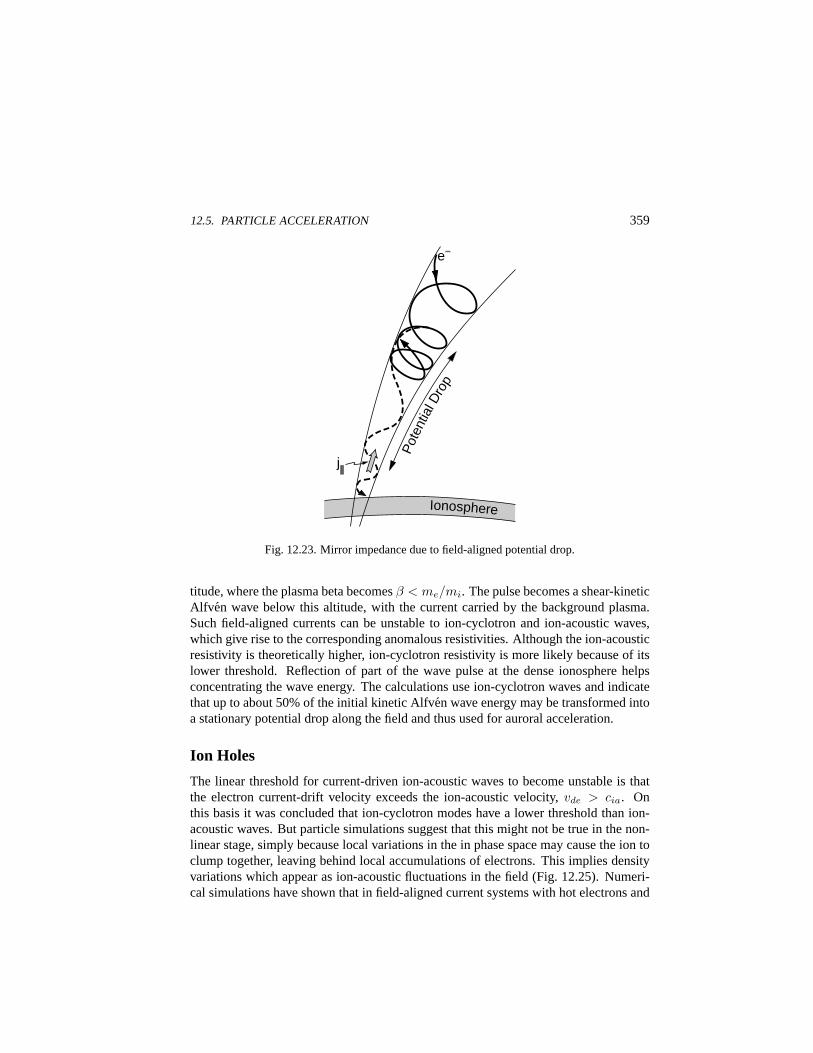
12.5. PARTICLE ACCELERATION 359
j||
Pot
entia
l Dro
p
Ionosphere
e−
Fig. 12.23. Mirror impedance due to field-aligned potential drop.
titude, where the plasma beta becomesβ < me/mi. The pulse becomes a shear-kineticAlfv en wave below this altitude, with the current carried by the background plasma.Such field-aligned currents can be unstable to ion-cyclotron and ion-acoustic waves,which give rise to the corresponding anomalous resistivities. Although the ion-acousticresistivity is theoretically higher, ion-cyclotron resistivity is more likely because of itslower threshold. Reflection of part of the wave pulse at the dense ionosphere helpsconcentrating the wave energy. The calculations use ion-cyclotron waves and indicatethat up to about 50% of the initial kinetic Alfven wave energy may be transformed intoa stationary potential drop along the field and thus used for auroral acceleration.
Ion Holes
The linear threshold for current-driven ion-acoustic waves to become unstable is thatthe electron current-drift velocity exceeds the ion-acoustic velocity,vde > cia. Onthis basis it was concluded that ion-cyclotron modes have a lower threshold than ion-acoustic waves. But particle simulations suggest that this might not be true in the non-linear stage, simply because local variations in the in phase space may cause the ion toclump together, leaving behind local accumulations of electrons. This implies densityvariations which appear as ion-acoustic fluctuations in the field (Fig. 12.25). Numeri-cal simulations have shown that in field-aligned current systems with hot electrons and
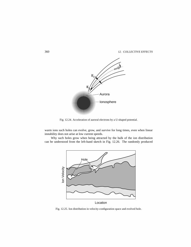
360 12. COLLECTIVE EFFECTS
Ionosphere
E⊥
Aurora
j||
E||
Fig. 12.24. Acceleration of auroral electrons by a U-shaped potential.
warm ions such holes can evolve, grow, and survive for long times, even when linearinstability does not arise at low current speeds.
Why such holes grow when being attracted by the bulk of the ion distributioncan be understood from the left-hand sketch in Fig. 12.26. The randomly produced
Hole
Location
Ion
Vel
ocity
Fig. 12.25. Ion distribution in velocity-configuration space and evolved hole.
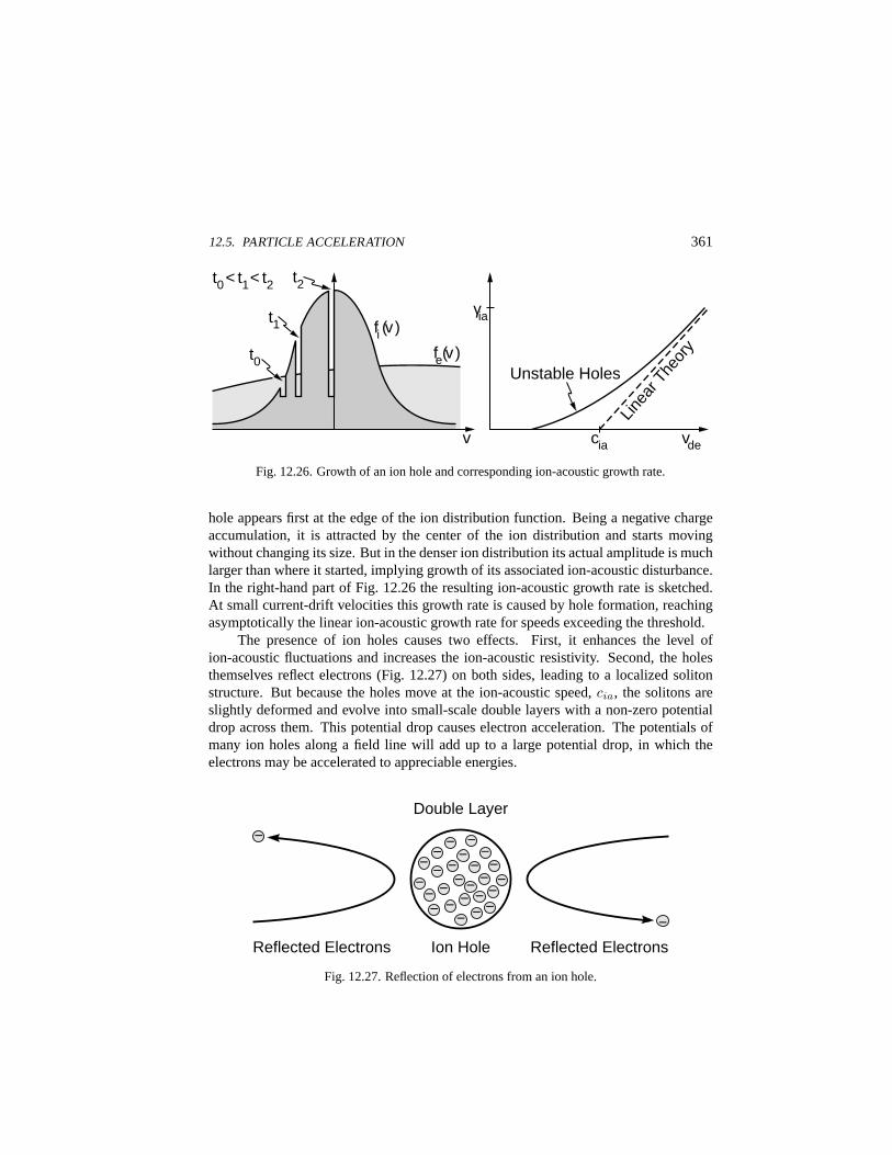
12.5. PARTICLE ACCELERATION 361
γia
cia vde
Unstable Holes
v
fe(v )
fi (v )
t0
t1
t2 t0< t1< t2
Line
arTh
eory
Fig. 12.26. Growth of an ion hole and corresponding ion-acoustic growth rate.
hole appears first at the edge of the ion distribution function. Being a negative chargeaccumulation, it is attracted by the center of the ion distribution and starts movingwithout changing its size. But in the denser ion distribution its actual amplitude is muchlarger than where it started, implying growth of its associated ion-acoustic disturbance.In the right-hand part of Fig. 12.26 the resulting ion-acoustic growth rate is sketched.At small current-drift velocities this growth rate is caused by hole formation, reachingasymptotically the linear ion-acoustic growth rate for speeds exceeding the threshold.
The presence of ion holes causes two effects. First, it enhances the level ofion-acoustic fluctuations and increases the ion-acoustic resistivity. Second, the holesthemselves reflect electrons (Fig. 12.27) on both sides, leading to a localized solitonstructure. But because the holes move at the ion-acoustic speed,cia, the solitons areslightly deformed and evolve into small-scale double layers with a non-zero potentialdrop across them. This potential drop causes electron acceleration. The potentials ofmany ion holes along a field line will add up to a large potential drop, in which theelectrons may be accelerated to appreciable energies.
−
Double Layer
Ion Hole Reflected Electrons Reflected Electrons
− − − −
− − − − −
− −
− −
− − −
− − −
− − − −
−
−
−
Fig. 12.27. Reflection of electrons from an ion hole.
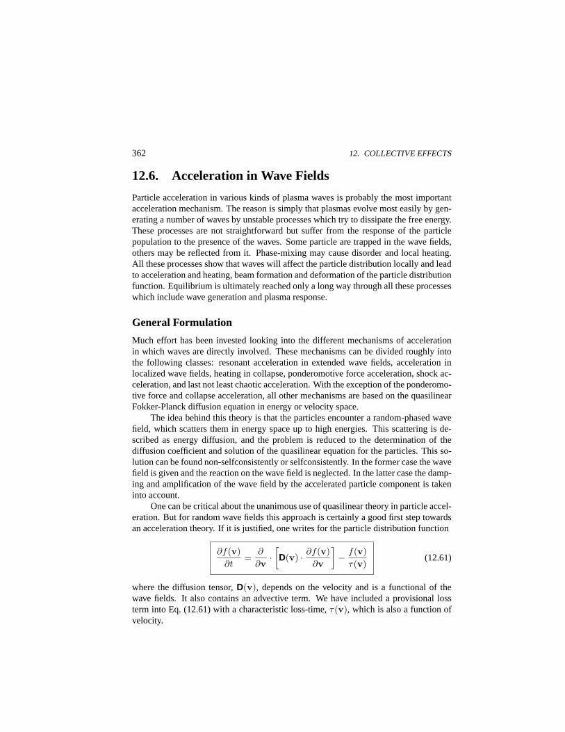
362 12. COLLECTIVE EFFECTS
12.6. Acceleration in Wave Fields
Particle acceleration in various kinds of plasma waves is probably the most importantacceleration mechanism. The reason is simply that plasmas evolve most easily by gen-erating a number of waves by unstable processes which try to dissipate the free energy.These processes are not straightforward but suffer from the response of the particlepopulation to the presence of the waves. Some particle are trapped in the wave fields,others may be reflected from it. Phase-mixing may cause disorder and local heating.All these processes show that waves will affect the particle distribution locally and leadto acceleration and heating, beam formation and deformation of the particle distributionfunction. Equilibrium is ultimately reached only a long way through all these processeswhich include wave generation and plasma response.
General Formulation
Much effort has been invested looking into the different mechanisms of accelerationin which waves are directly involved. These mechanisms can be divided roughly intothe following classes: resonant acceleration in extended wave fields, acceleration inlocalized wave fields, heating in collapse, ponderomotive force acceleration, shock ac-celeration, and last not least chaotic acceleration. With the exception of the ponderomo-tive force and collapse acceleration, all other mechanisms are based on the quasilinearFokker-Planck diffusion equation in energy or velocity space.
The idea behind this theory is that the particles encounter a random-phased wavefield, which scatters them in energy space up to high energies. This scattering is de-scribed as energy diffusion, and the problem is reduced to the determination of thediffusion coefficient and solution of the quasilinear equation for the particles. This so-lution can be found non-selfconsistently or selfconsistently. In the former case the wavefield is given and the reaction on the wave field is neglected. In the latter case the damp-ing and amplification of the wave field by the accelerated particle component is takeninto account.
One can be critical about the unanimous use of quasilinear theory in particle accel-eration. But for random wave fields this approach is certainly a good first step towardsan acceleration theory. If it is justified, one writes for the particle distribution function
∂f(v)∂t
=∂
∂v·[D(v) · ∂f(v)
∂v
]− f(v)
τ(v)(12.61)
where the diffusion tensor,D(v), depends on the velocity and is a functional of thewave fields. It also contains an advective term. We have included a provisional lossterm into Eq. (12.61) with a characteristic loss-time,τ(v), which is also a function ofvelocity.
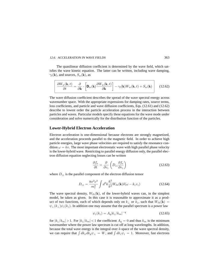
12.6. ACCELERATION IN WAVE FIELDS 363
The quasilinear diffusion coefficient is determined by the wave field, which sat-isfies the wave kinetic equation. The latter can be written, including wave damping,γl(k), and sources,Sw(k), as
∂Ww(k, t)∂t
=∂
∂k·[Dw(k)
∂Ww(k, t)∂k
]− γl(k)Ww(k, t) + Sw(k) (12.62)
The wave diffusion coefficient describes the spread of the wave spectral energy acrosswavenumber space. With the appropriate expressions for damping rates, source terms,loss coefficients, and particle and wave diffusion coefficients, Eqs. (12.61) and (12.62)describe to lowest order the particle acceleration process in the interaction betweenparticles and waves. Particular models specify these equations for the wave mode underconsideration and solve numerically for the distribution function of the particles.
Lower-Hybrid Electron Acceleration
Electron acceleration is one-dimensional because electrons are strongly magnetized,and the acceleration proceeds parallel to the magnetic field. In order to achieve highparticle energies, large wave phase velocities are required to satisfy the resonance con-dition ω = kv. The most important electrostatic wave with high parallel phase velocityis the lower-hybrid wave. Restricting to parallel energy diffusion only, the parallel elec-tron diffusion equation neglecting losses can be written
∂fe
∂t=
∂
∂v‖
(D‖‖
∂fe
∂v‖
)(12.63)
whereD‖‖ is the parallel component of the electron diffusion tensor
D‖‖ =8π2e2
m2e
∫d3k
k2‖
k2Wlh(k)δ(ω − k‖v‖) (12.64)
The wave spectral density,Wlh(k), of the lower-hybrid waves can, in the simplestmodel, be taken as given. In this case it is reasonable to approximate it as a prod-uct of two functions, each of which depends only onk⊥ or k‖, such thatWlh(k) =ψ⊥(k⊥)ψ‖(k‖). In addition one may assume that the parallel spectrum is a power law
ψ‖(k‖) = Aq|k‖/km|−q (12.65)
for |k‖/km|> 1. For |k‖/km|< 1 the coefficientAq = 0 and thuskm is the minimumwavenumber where the power law spectrum is cut off at long wavelengths. In addition,because the total wave energy is the integral overk-space of the wave spectral density,we can require that
∫dkxdkyψ⊥ = W , and
∫dk‖ψ‖ = 1. Moreover, fast electrons
364 12. COLLECTIVE EFFECTS
have speeds larger than the group velocity of the lower-hybrid wave,vgr‖ ¿ v‖. Thusthe parallel diffusion coefficient can be approximated as
D‖‖ ≈ Aq|v‖|−3|kmv‖/ω|q (12.66)
whereAq = 2πω2pev
20WAq/men0 is another coefficient. We now set formallyω =
k⊥v0 and introduce normalized parallel velocities and times according tou = v‖/vthe
andτ = t(Aq/v5the)|kmvthe/ω|q, which allows us to rewrite the parallel electron ve-
locity space diffusion equation into the simple form
∂fe(u, τ)∂τ
=∂
∂u
(1
|u|3−q
∂fe(u, t)∂u
)(12.67)
This equation must be solved under an appropriate initial condition. For example, onecan assume that the initial distribution function at timeτ = 0 is a Maxwellian
f0(u) = π−1/2n0 exp(−u2) (12.68)
It should be noted that the above equation has a trivial solution forq = 3, becausefor the corresponding spectrum the diffusion coefficient is constant, and the solution issimply that of a dispersing heat pulse. However, this solution is of little interest, sinceit is inappropriate for nearly all conditions encountered in space plasmas. The solutionof the diffusion equation for generalq can be constructed with the help of the Laplacetransform technique. It is represented in the form of an integral
fe(u, τ) =∫ ∞
0
du′gq(u, u′, τ)f0(u′) (12.69)
where the Green’s function is determined from the Laplace transform of the above one-dimensional electron diffusion equation. One finds
gq(u, u′, τ) =(uu′)2−q/2
(5− q)τI−ν(η) exp
[−u5−q + u′5−q
(5− q)2τ
](12.70)
with the following abbreviationsν = (4−q)/(5−q) andη = 2(uu′)(5−q)/2/(5−q)2τ ,andI−ν a Bessel function.
For any given parallel power law index,q, this expression shows a complicateddependence on velocity and time, but as is typical for diffusive processes, the entiredistribution will decrease with time and will at the same time broaden inu-space withincreasing time. This implies that the initial Maxwellian will spread out inu to generatea long extended tail indicating continuous acceleration of electrons to high energies.The long-time behavior for a power law index ofq = 4, say, is found to evolve like
fe(u, τ) ≈ n0τ−1 exp(−|u|/τ) (12.71)
This function decays much less steeply with velocity than the Gaussian function.
12.6. ACCELERATION IN WAVE FIELDS 365
Localized Lower-Hybrid Waves
The theory presented above shows that extended lower-hybrid wave fields may, in con-tinuous interaction with an electron distribution, generate tails on the distribution andaccelerate electrons to high energies. But this model is unrealistic, because electronsmove rather fast along the magnetic field and will readily leave from the region occu-pied by the waves. In addition, lower hybrid waves of high intensity may evolve intolocalized wave packets, with the interaction between electrons and waves limited to thetransition time of the electrons across the packets which may be described as cavitonsfilled with lower-hybrid plasmons. The observation of such lower-hybrid cavitons incorrelation with the appearance of auroral electron beams strongly suggests that accel-eration in localized wave fields is more important in most cases than acceleration inextended fields.
Localization of the wave field considerably complicates the simple theory of theprevious section. Progress can be made by assuming that the electric wave field enteringthe diffusion coefficient is derived from an electrostatic potential
Φ(ξ, t) = (2π)−1/2V (ξ, t)∑
k
Q(k) exp i[kξ − ω(k)t] (12.72)
with V (ξ, t) the slowly variable envelope potential, andξ the spatial coordinate parallelto the direction of the lower-hybrid wave vector. The functionQ(k) is thek-spectrum ofthe waves trapped inside the caviton. If the wave is a single mode, then this spectrum isa delta-function, and thek-dependence is solely given by the transform of the envelope.Since the caviton moves at speedu0, the coordinate in the moving frame isx = ξ −u0t cos θ, andθ is the angle against the magnetic field. This propagation speed is nearlyparallel to the magnetic field.
In order to determine the diffusion coefficient we need the spectral energy densityof the waves. This can be calculated from the correlation function knowing the waveelectric field
E(x, t) = −(2π)−1/2V (x)∑
k
R(k) exp i(kx−$t) (12.73)
with $ = ω − ku0 cos θ andR = ikQ. For the envelope we assume the cavitonfunction
V (x) = A sech(bx) (12.74)
But for technical purposes it is simpler to actually use a corresponding Gaussian profile,V (x) = A exp(−bx2), which has a similar shape. Calculating the correlation functionof the total lower-hybrid wave field
C(x, t) =∫ ∫
dζdτE∗(ζ, τ)E(x + ζ, t + τ) (12.75)
366 12. COLLECTIVE EFFECTS
one finds that the correlation function can be represented as
C(x, t) = C0g(√
2a, x/2L⊥)∑
k
|R(k)|2 exp i(kx−$t) (12.76)
whereC0 = A2/8(2aπ)1/2, the functiong is defined as
g(v, w) = erf[v(w + 1)]− erf[v(w − 1)] exp(−v2|w|2) (12.77)
anda = bL2⊥. The length scaleL⊥ is the perpendicular scale of the caviton as obtained
from the nonlinear Schrodinger theory. It is related to the amplitude,A, by Eq. (11.58)
A2L2⊥
∑
k
|Q(k)|2 ≈ (12λDikBTe/e)2 (12.78)
The next step is to take the Fourier transform of the correlation function to obtain thespectral energy density as
W (κ, Ω) = W0
∑
k
|R(k)|2δ(Ω−$)g(a1/2, w) exp(−a|w|2) (12.79)
and from it to construct the parallel electron velocity space diffusion coefficient
D(v) =W0 cos θ
2|v|∑
k
|R(k)|2g(a1/2, γ
)exp(−1|γ|2) (12.80)
where we used the abbreviations,W0 = A2L⊥/8a(2π)1/2, andw = i(k − κ)L⊥/2a.In addition,γ = iαkL⊥/2a andα = [ω − k(u0 + v) cos θ]/kv cos θ.
This diffusion coefficient is shown in the left-hand part of Fig. 12.28 as a functionof the normalized electron velocity,v/vthe. It peaks well outside the center of theelectron distribution, thus leaving the lowest energy electrons unaffected since they donot come into resonance with the waves trapped in the caviton. Hence, cavitons orlocalized waves cause different electron dynamics than extended wave fields. Only arelatively narrow range of electron energies will be accelerated by the localized packets,since an electron can spend only finite time in the caviton.
The above diffusion coefficient can be used to solve the diffusion equation forelectrons. A Monte-Carlo simulation solution using many electrons initially distributedas a parallel Maxwellian is shown in the right-hand panel of Fig. 12.28. In the long-time limit the distribution function starts exhibiting well expressed maxima outside themain peak. These maxima are at about 16 times the thermal energy of the electrons, inrough agreement with observations. Also, the shape of the spectrum resembles thosemeasured in the auroral magnetosphere.
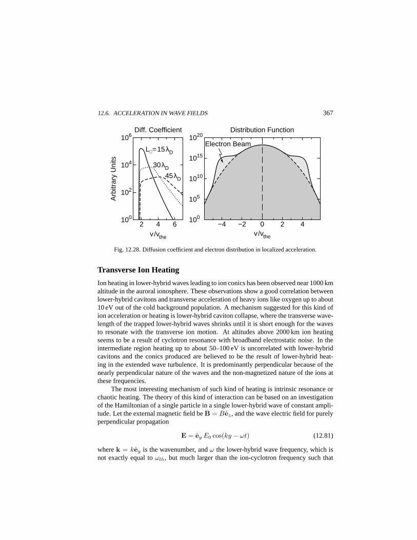
12.6. ACCELERATION IN WAVE FIELDS 367
1020
1010
100
105
1015
Distribution Function
Electron Beam
0 −2 −4 2 4 v /vthe
Diff. Coefficient
L⊥=15λD
30λD
45λD
v /vthe
2 4 6 100
102
104
106
Arb
itrar
y U
nits
Fig. 12.28. Diffusion coefficient and electron distribution in localized acceleration.
Transverse Ion Heating
Ion heating in lower-hybrid waves leading to ion conics has been observed near 1000 kmaltitude in the auroral ionosphere. These observations show a good correlation betweenlower-hybrid cavitons and transverse acceleration of heavy ions like oxygen up to about10 eV out of the cold background population. A mechanism suggested for this kind ofion acceleration or heating is lower-hybrid caviton collapse, where the transverse wave-length of the trapped lower-hybrid waves shrinks until it is short enough for the wavesto resonate with the transverse ion motion. At altitudes above 2000 km ion heatingseems to be a result of cyclotron resonance with broadband electrostatic noise. In theintermediate region heating up to about 50–100 eV is uncorrelated with lower-hybridcavitons and the conics produced are believed to be the result of lower-hybrid heat-ing in the extended wave turbulence. It is predominantly perpendicular because of thenearly perpendicular nature of the waves and the non-magnetized nature of the ions atthese frequencies.
The most interesting mechanism of such kind of heating is intrinsic resonance orchaotic heating. The theory of this kind of interaction can be based on an investigationof the Hamiltonian of a single particle in a single lower-hybrid wave of constant ampli-tude. Let the external magnetic field beB = Bez, and the wave electric field for purelyperpendicular propagation
E = ey E0 cos(ky − ωt) (12.81)
wherek = key is the wavenumber, andω the lower-hybrid wave frequency, which isnot exactly equal toωlh, but much larger than the ion-cyclotron frequency such that

368 12. COLLECTIVE EFFECTS
dy dt
dy dt
=ν
B y
Location of Resonance Kick
Fig. 12.29. A gyrating ion gets a kick at resonance.
ν = ω/ωgi À 1. Thus the ions behave nearly unmagnetized at these high frequencies,but they still perform a gyratory motion. At some places on this orbit, where the un-magnetized resonance condition,ω = k · v, is satisfied, they experience a kick in theirmotion extracting energy out of the wave, and become accelerated in the perpendiculardirection. Thereby they increase their gyroradius on the expense of the wave amplitude.
We consider a non-selfconsistent problem in which the wave amplitude and energyare kept constant. Using normalized coordinates, with time normalized to1/ωgi, lengthto 1/k, and velocity toωgi/k, the Hamiltonian of the ions becomes
H = 12 [(px + y)2 + p2
y]− α sin(y − νt) (12.82)
The coefficientα controls the behavior of the ion motion. It is given by
α = kE0/ωgiB (12.83)
The momentum,px, is a constant, because the Hamiltonian does not depend onx.From this Hamiltonian it is possible to derive the equations of motion of the ion in
the lower-hybrid wave field. The first equation is simply
dx/dt = y (12.84)
The second equation is a driven oscillator equation
(d2y/dt2) + y = α cos(y − νt) (12.85)
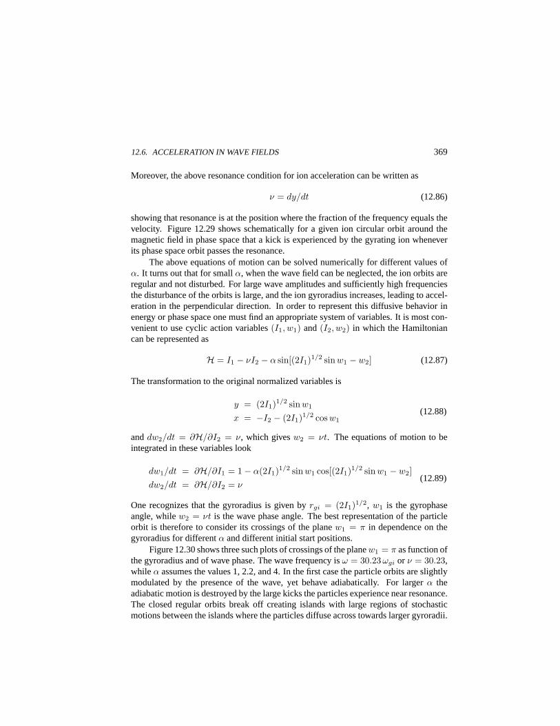
12.6. ACCELERATION IN WAVE FIELDS 369
Moreover, the above resonance condition for ion acceleration can be written as
ν = dy/dt (12.86)
showing that resonance is at the position where the fraction of the frequency equals thevelocity. Figure 12.29 shows schematically for a given ion circular orbit around themagnetic field in phase space that a kick is experienced by the gyrating ion wheneverits phase space orbit passes the resonance.
The above equations of motion can be solved numerically for different values ofα. It turns out that for smallα, when the wave field can be neglected, the ion orbits areregular and not disturbed. For large wave amplitudes and sufficiently high frequenciesthe disturbance of the orbits is large, and the ion gyroradius increases, leading to accel-eration in the perpendicular direction. In order to represent this diffusive behavior inenergy or phase space one must find an appropriate system of variables. It is most con-venient to use cyclic action variables(I1, w1) and(I2, w2) in which the Hamiltoniancan be represented as
H = I1 − νI2 − α sin[(2I1)1/2 sin w1 − w2] (12.87)
The transformation to the original normalized variables is
y = (2I1)1/2 sin w1
x = −I2 − (2I1)1/2 cosw1(12.88)
anddw2/dt = ∂H/∂I2 = ν, which givesw2 = νt. The equations of motion to beintegrated in these variables look
dw1/dt = ∂H/∂I1 = 1− α(2I1)1/2 sin w1 cos[(2I1)1/2 sin w1 − w2]dw2/dt = ∂H/∂I2 = ν
(12.89)
One recognizes that the gyroradius is given byrgi = (2I1)1/2, w1 is the gyrophaseangle, whilew2 = νt is the wave phase angle. The best representation of the particleorbit is therefore to consider its crossings of the planew1 = π in dependence on thegyroradius for differentα and different initial start positions.
Figure 12.30 shows three such plots of crossings of the planew1 = π as function ofthe gyroradius and of wave phase. The wave frequency isω = 30.23 ωgi or ν = 30.23,while α assumes the values 1, 2.2, and 4. In the first case the particle orbits are slightlymodulated by the presence of the wave, yet behave adiabatically. For largerα theadiabatic motion is destroyed by the large kicks the particles experience near resonance.The closed regular orbits break off creating islands with large regions of stochasticmotions between the islands where the particles diffuse across towards larger gyroradii.
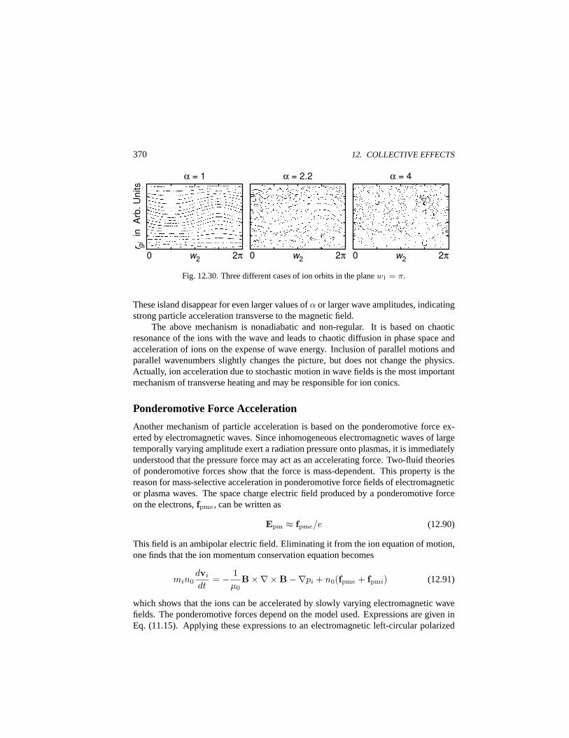
370 12. COLLECTIVE EFFECTS
r gi i
n A
rb. U
nits
0 w2 2π 0 w2 2π 0 w2 2π
α = 1 α = 2.2 α = 4
Fig. 12.30. Three different cases of ion orbits in the planew1 = π.
These island disappear for even larger values ofα or larger wave amplitudes, indicatingstrong particle acceleration transverse to the magnetic field.
The above mechanism is nonadiabatic and non-regular. It is based on chaoticresonance of the ions with the wave and leads to chaotic diffusion in phase space andacceleration of ions on the expense of wave energy. Inclusion of parallel motions andparallel wavenumbers slightly changes the picture, but does not change the physics.Actually, ion acceleration due to stochastic motion in wave fields is the most importantmechanism of transverse heating and may be responsible for ion conics.
Ponderomotive Force Acceleration
Another mechanism of particle acceleration is based on the ponderomotive force ex-erted by electromagnetic waves. Since inhomogeneous electromagnetic waves of largetemporally varying amplitude exert a radiation pressure onto plasmas, it is immediatelyunderstood that the pressure force may act as an accelerating force. Two-fluid theoriesof ponderomotive forces show that the force is mass-dependent. This property is thereason for mass-selective acceleration in ponderomotive force fields of electromagneticor plasma waves. The space charge electric field produced by a ponderomotive forceon the electrons,fpme, can be written as
Epm ≈ fpme/e (12.90)
This field is an ambipolar electric field. Eliminating it from the ion equation of motion,one finds that the ion momentum conservation equation becomes
min0dvi
dt= − 1
µ0B×∇×B−∇pi + n0(fpme + fpmi) (12.91)
which shows that the ions can be accelerated by slowly varying electromagnetic wavefields. The ponderomotive forces depend on the model used. Expressions are given inEq. (11.15). Applying these expressions to an electromagnetic left-circular polarized
12.6. ACCELERATION IN WAVE FIELDS 371
ion wave, the acceleration parts in the ion equation of motion can be written as
min0dvi‖
dt= − ω2
pi
ω ωgi
[ω
ω − ωgi∇‖ − k
ω
(1− ω2
gi
(ω − ωgi)2
)∂
∂t
]WE
min0dvi⊥dt
= −ω2pe
ω2ge
[1− me
mi
ω2ge
(ω − ωgi)2
]∇⊥WE
(12.92)
Obviously, there is acceleration of ions in the field of an electromagnetic ion-cyclotronwave with the acceleration acting in both directions. Parallel to the field it will resultin acceleration, the transverse effect is heating. The above equations suggest that ionacceleration is significantly enhanced when the frequency is close to the ion-cyclotronfrequency. But this conclusion must be taken with care because close to the cyclotronresonance the ponderomotive effect is changed by other kinetic effects.
Diffuse Fermi Acceleration
Very often one observes ion distributions which are not simple beams but diffuselyaccelerated distributions. We have mentioned such examples in connection with ion re-flection and further evolution of the so-called kidney distributions into diffuse ring dis-tributions at the Earth’s bow shock wave in the quasi-parallel foreshock region wherelarge-amplitude low-frequency magnetic turbulence evolves into shocklets. The in-teraction of this turbulence with the non-isotropic ion distribution is believed to leadto strong ion heating and ion acceleration in these cases. This process is usually re-ferred to assecond-order Fermiacceleration, but in essence it is stochastic accelerationin extended large-amplitude low-frequency electromagnetic waves propagating in thewhistler or ion-cyclotron band.
This process is formally described by Eqs. (12.61) and (12.62). The accelerationprocess is quasilinear. In order to solve these equations, assumptions must be intro-duced about the damping, growth, and loss rates of particles and waves and about theparticle and wave diffusion coefficients. So far these assumptions have been basedonly on simple considerations, and nonlinear effects have never been taken into ac-count. Usually a spatial diffusion coefficient parallel to the magnetic field,κ‖ =〈(∆s)2〉/(2∆t), is introduced. This coefficient gives the diffusive escape time of theparticles asτd ≈ L2/8κ‖, whereL = 2∆s is the length of the system along the mag-netic field. An approximation forκ‖ is obtained from pitch angle diffusion theory. Theresulting approximative expression for the particle loss-time is
τd =9π2e2
4c2
L2
m2i v
3
∞∫
k0
dk‖k‖
(1− k2
0
k2‖Ww(k‖
)(12.93)
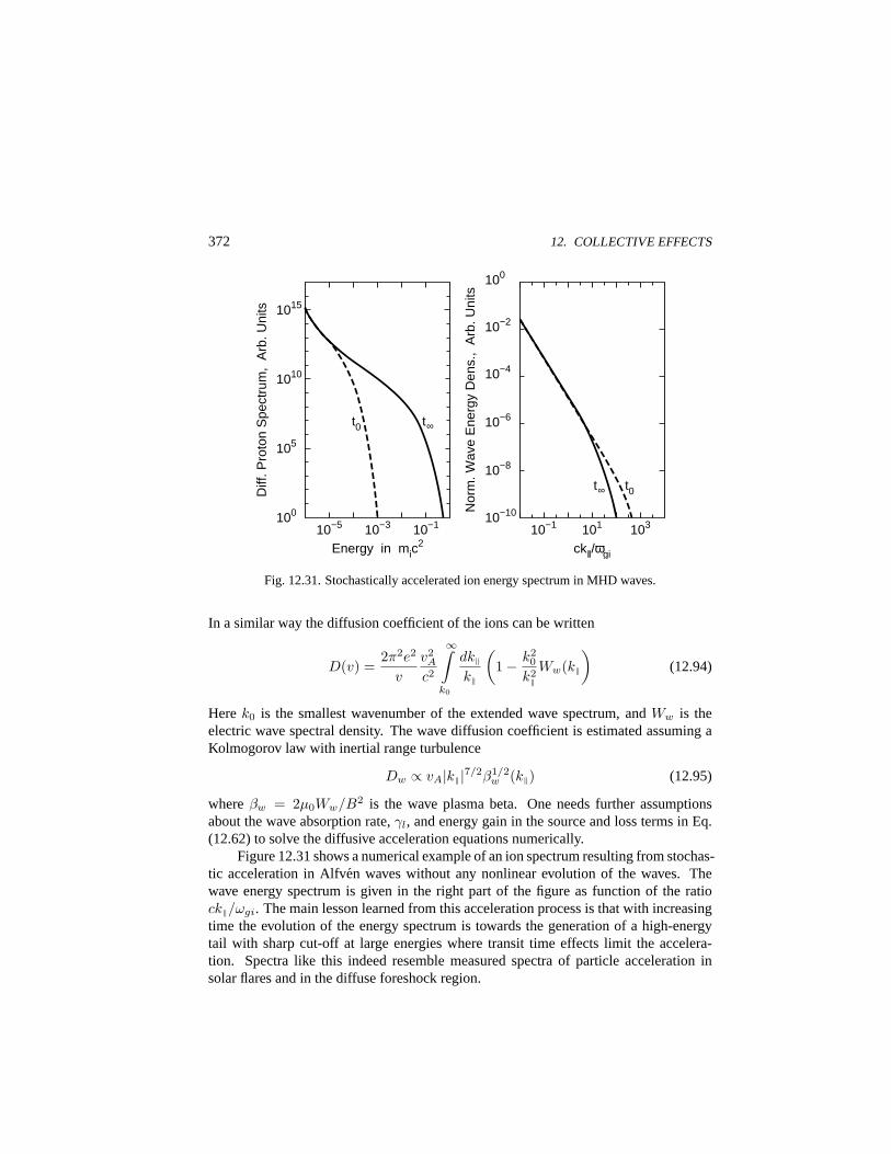
372 12. COLLECTIVE EFFECTS
Energy in mic2
10−5 10−3 10−1 10−1 101 103
ck ||/ωgi
100
105
1010
1015
Diff
. Pro
ton
Spe
ctru
m,
Arb
. Uni
ts
10−10
10−8
10−6
10−4
Nor
m. W
ave
Ene
rgy
Den
s.,
Arb
. Uni
ts
10−2
100
t0 t∞
t∞ t0
Fig. 12.31. Stochastically accelerated ion energy spectrum in MHD waves.
In a similar way the diffusion coefficient of the ions can be written
D(v) =2π2e2
v
v2A
c2
∞∫
k0
dk‖k‖
(1− k2
0
k2‖Ww(k‖
)(12.94)
Herek0 is the smallest wavenumber of the extended wave spectrum, andWw is theelectric wave spectral density. The wave diffusion coefficient is estimated assuming aKolmogorov law with inertial range turbulence
Dw ∝ vA|k‖|7/2β1/2w (k‖) (12.95)
whereβw = 2µ0Ww/B2 is the wave plasma beta. One needs further assumptionsabout the wave absorption rate,γl, and energy gain in the source and loss terms in Eq.(12.62) to solve the diffusive acceleration equations numerically.
Figure 12.31 shows a numerical example of an ion spectrum resulting from stochas-tic acceleration in Alfven waves without any nonlinear evolution of the waves. Thewave energy spectrum is given in the right part of the figure as function of the ratiock‖/ωgi. The main lesson learned from this acceleration process is that with increasingtime the evolution of the energy spectrum is towards the generation of a high-energytail with sharp cut-off at large energies where transit time effects limit the accelera-tion. Spectra like this indeed resemble measured spectra of particle acceleration insolar flares and in the diffuse foreshock region.
12.6. ACCELERATION IN WAVE FIELDS 373
The current theory is semi-selfconsistent. It takes into account the modificationof the spectrum and particle fluxes under the interaction, but it introduces severe as-sumptions about the spatial extent of the waves and about the growth, damping, loss,and diffusion rates. Nevertheless, it explains the generation of very high energy tails asobserved in foreshocks, solar flares, and in cosmic rays.
Concluding Remarks
We have excluded many facts and fields from this last chapter, mainly because of lackof space. In particular, we regret not having been able to review slow and intermediateshock theories, which all still are under ongoing discussion. Also shock accelerationin its two variants, first-order Fermi and shock drift acceleration, has been left aside.In spite of their wide application in cosmic ray physics and astrophysics these theoriesform the simpler part of all acceleration mechanisms.
Further Reading
The general theory of transport coefficients is summarized in [1]. The calculation ofanomalous transport coefficients is described in [2] and [4]. The calculation of formfactors is given in [3]. Thresholds of ion-acoustic turbulence were determined by Kindeland Kennel,J. Geophys. Res.76 (1971) 3055. Ion-cyclotron collision frequencies aregiven by Dum and Dupree,Phys. Fluids13 (1970) 2064. Ion-acoustic resistivity is thesubject of Dum,Phys. Fluids, 21 (1978) 945. Strongly turbulent Langmuir collisionfrequencies are found in Sagdeev,Rev. Mod. Phys., 51 (1979) 1.
Observational information on shocks is found in [7] and [9]. The older theoriesof laminar and turbulent shocks are discussed in [8], more recent information is foundin [6]. The various critical Mach numbers are discussed by Kennel et al. in [7]. Mi-croinstabilities and their effects on shocks are found in Wu et al.,Space Sci. Rev., 37(1984) 63. Ion distributions in the foreshock are given in Sckopke et al.,J. Geophys.Res., 88 (1983) 6121. Measured ion-cyclotron spectra are presented by Sckopke et al.,J. Geophys. Res., 95 (1990) 6337. Waves in the magnetosheath are summarized by La-combe and Belmont in [6]. A summary of electron distribution functions in and nearshocks is given by Feldman in [9]. Upstream waves, slams and shocklets and their rolein reformation are discussed by Scholer,J. Geophys. Res., 98 (1993) 47.
For the kinetic Alfven wave mechanism of auroral acceleration we followed Lysakand Dum,J. Geophys. Res., 88 (1983) 365. Ion hole formation is taken from Tetreault,J. Geophys. Res., 96 (1991) 3549 and Gray et al.,Geophys. Res. Lett., 18 (1991) 1675.For the acceleration in extended lower-hybrid wave fields see Wu et al.,J. PlasmaPhys., 25 (1981) 391. The theory of localized electron acceleration follows work byDubouloz et al.,Geophys. Res. Lett., 22 (1995) 2969. Perpendicular ion heating is the
374 12. COLLECTIVE EFFECTS
subject of Karney,Phys. Fluids, 21 (1978) 1584 &22 (1979) 2188. Ion acceleration inextended wave fields is discussed by Miller and Roberts,Astrophys. J., 452(1995) 912.Ponderomotive force acceleration was mentioned first by Pottelette et al. in [5].
[1] S. I. Braginskii, inReviews of Plasma Physics 1, ed. M. A. Leontovich (Consul-tants Bureau, New York, 1965), p. 205.
[2] A. A. Galeev and R. Z. Sagdeev, inReviews of Plasma Physics 7, ed. M. A. Leon-tovich (Consultants Bureau, New York, 1979), p. 1.
[3] S. Ichimaru,Basic Principles of Plasma Physics(W. A. Benjamin, Reading,1973).
[4] B. B. Kadomtsev,Plasma Turbulence(Academic Press, New York, 1965).
[5] R. L. Lysak (ed.),Auroral Plasma Dynamics(American Geophysical Union,Washington, 1993).
[6] C. T. Russell (ed.),Advances of Space Research 15: Physics of CollisionlessShocks(Pergamon, Oxford, 1995).
[7] R. G. Stone and B. T. Tsurutani (eds.),Collisionless Shocks in the Heliosphere: ATutorial Review(American Geophysical Union, Washington, 1985).
[8] D. A. Tidman and N. A. Krall,Shock Waves in Collisionless Plasmas(Wiley In-terscience, New York, 1971).
[9] B. T. Tsurutani and R. G. Stone (eds.),Collisionless Shocks in the Heliosphere:Reviews of Current Research(American Geophysical Union, Washington, 1985).
[10] V. N. Tsytovich,Nonlinear Effects in Plasmas(Plenum Press, New York, 1970).

Epilogue
There would be infinitely more to say about observation and theory of space and astro-physical plasmas. But an introductory text must close at some point. In our two books,Basic Space Plasma PhysicsandAdvanced Space Plasma Physics, we have tried to givean overview of the current state of the art in space plasma physics on a level which wehope is accessible to the student and to the beginning researcher. Clearly, both volumesshould be taken together in order to get a relatively complete picture of space plasmaphysics, reaching from the elementary level of particle motion in crossed electric andmagnetic fields through the state of plasma equilibria up to the more sophisticated levelof nonlinear plasma theory.
As far as the available space allowed, we tried to follow the demand of theoreticalrigor. However, the reader will find that this intention has been violated at severalplaces, where we skipped the derivation and went on to a verbal description. In all thesecases we have put effort into a relatively clear description of the physics involved and adiscussion of its consequences. We feel that sometimes such a choice is more valuablethan being lost in the rigorous but complicated mathematical jungle. In most of thosecases we tried, however, to write down the fundamental mathematical expressions.
As the authors of this text we are left with the unpleasant feeling that we haveonly touched the problems, skipped a large number of important and interesting effects,which we either felt to go too far beyond an introductory presentation or, worse, wehave not been aware of. In the latter case we would be grateful for hints which fieldsshould be included in any possible forthcoming edition. However, the inevitable incom-pleteness of this course may be compensated by consulting the book edited by M. G.Kivelson and C. T. Russell,Introduction to Space Physics. There the reader will find amore phenomenological description of many space plasma phenomena which we havementioned (or neglected). In a sense the two approaches to space plasma physics giventhere and here complement each other.
Numerical simulations are the largest field which we have excluded from this in-troduction to space plasma physics. Contemporary theoretical space plasma physics isto a large part based on numerical simulations. The great advantage of simulations isthat they include the nonlinear evolution of the simulated system in a quite natural way.Thus they provide deep insight into the evolution of many phenomena which sometimes
375

376 EPILOGUE
cannot even be formulated analytically. There are many examples, especially involv-ing inhomogeneities and nonlinearities, where problems could only be solved by thesimulation technique.
Interestingly, numerical simulations create a different view of the phenomena. Nu-merical simulation can be taken as an experiment done not on real but model plasmas.Space plasma physics has used this possibility in order to investigate those aspects ofwhich real experiments in space can give only sporadic information. This tendencyis interesting and challenging, because for a really deep understanding of the variousnatural and simulated phenomena the combination of observation, simulation, and an-alytical investigation is required. To provide the basis for the latter was the intentionof the writing of this book. But in application to real problems the contemporary re-searcher will typically enter numerical simulations. A small number of books where anintroduction into numerical simulation technique can be found have been mentioned inthe last few chapters.
Index
absolute instability, 93acceleration, 362adiabatic collapse, 304Alfv en soliton, 268Alfv en wave, 44, 52, 56, 118, 137, 146ambipolar diffusion, 329ambipolar field, 370anisotropy-driven instability, 105anomalous diffusion, 329anomalous resistivity, 318, 358auroral acceleration, 356auroral arc, 49auroral electrons, 100, 208, 358auroral folds, 49auroral ionosphere, 79, 313auroral kilometric radiation, 127, 325
beam instability, 27, 70, 80, 81, 114beam turbulence, 186Bernstein wave, 85, 91BGK modes, 181Bohm diffusion, 330Boltzmann law, 285boundary layer, 331bow shock, 22, 74, 118, 312, 326broadband noise, 111, 127bump-in-tail distribution, 70bump-in-tail instability, 298Buneman collision, 321Buneman instability, 22, 321Burgers equation, 245, 250, 287
carrier wave, 293caviton, 244, 283caviton burn-out, 308caviton collapse, 302caviton dimension, 302cavity, 293chaotic acceleration, 370Cherenkov emission, 14, 101
coalescence instability, 169coherent interaction, 220collapse scaling, 304, 306collapse speed, 304collective interaction, 5collision frequency, 38, 82, 318, 320collisional plasma, 2collisionless plasma, 3collisionless reconnection, 150, 160cometary waves, 119convection, 4convective instability, 93coplanarity violation, 346counterstreaming instability, 27critical current, 324critical electric field, 285, 322, 326critical Mach number, 337current saturation, 322current-driven instability, 75, 84, 87cyclotron emission, 121cyclotron frequency, 2cyclotron resonance, 106
damping rate, 10de Hoffmann-Teller frame, 345Debye length, 1Debye screening, 3density depletion, 315diamagnetic drift, 5, 135, 139dielectric tensor, 8diffuse acceleration, 371diffuse aurora, 99, 111diffusion coefficient, 38, 187, 191, 199diffusion region, 146dispersion relation, 7, 13, 290distribution function, 6double layer, 264, 315, 358Dreicer field, 323drift instability, 136drift kinetic equation, 133, 330
377
378 INDEX
drift wave, 129, 133, 136, 231drift wave instability, 129, 133drift wave soliton, 277drift wave turbulence, 231, 277drift-Alfv en instability, 137drift-cyclotron instability, 136
E-region ionosphere, 37electron acceleration, 312, 366electron beam, 312, 313, 315, 366electron diffusion, 331electron friction, 319electron-acoustic instability, 82electron-acoustic soliton, 264electron-acoustic wave, 82, 264, 351electron-cyclotron collision, 324electron-cyclotron instability, 91, 108, 120,
196, 208electron-cyclotron turbulence, 196, 208electron-cyclotron wave, 91, 108, 196, 208,
324electrostatic hiss, 100, 127energy principle, 60enstrophy, 233entropy, 334, 353entropy function, 230envelope caviton, 293, 296, 304envelope soliton, 285equation of motion, 4equatorial electrojet, 42E×B drift, 4explosive instability, 226extraordinary mode, 120, 127
F-region ionosphere, 37Farley-Buneman instability, 41field-aligned current, 63, 79, 85, 324, 360firehose instability, 51, 212fluid equations, 6flute instability, 31flux ropes, 174flux transfer event, 169, 172Fokker-Planck equation, 188, 362foreshock, 22, 84, 118, 344, 350, 371, 373four-wave interaction, 295free energy, 11
gentle beam instability, 70, 186, 298, 307gravitational instability, 31
group velocity, 7growth rate, 10, 12, 13guiding center, 4gyroemission, 121gyroradius, 3
Hamilton-Jacobi equation, 294Harris sheet, 160, 170Hasegawa-Mima equation, 232heat flux instability, 81helical instability, 65
incoherent interaction, 227induced emission, 14induction equation, 144inertial length, 104, 112interchange instability, 31interface instability, 351inverse caviton, 298inverse scattering method, 255inverted V events, 357ion acceleration, 344ion beam, 344, 348, 354ion beam instability, 27, 114, 349ion conics, 357, 367ion heating, 312, 367ion holes, 359ion reflection, 342ion-acoustic collision, 321ion-acoustic instability, 75, 201, 361ion-acoustic soliton, 261ion-acoustic wave, 53, 75, 201, 261, 298,
351ion-cyclotron collision, 324, 359ion-cyclotron diffusion, 330ion-cyclotron instability, 84, 94, 111, 202,
324ion-cyclotron wave, 85, 94, 111, 136, 202,
324, 352, 371ion-ion instability, 114, 116, 349
Joule heating, 319, 337
kappa distribution, 356Kelvin-Helmholtz instability, 43kidney beam distribution, 348kinetic Alfven diffusion, 330kinetic Alfven wave, 47, 49, 268, 315kinetic equation, 5

INDEX 379
kink instability, 64Kolmogorov spectrum, 309Korteweg-de Vries equation, 246, 254, 266,
287, 294, 297
laminar shock, 337Landau damping, 15, 70, 78, 179, 302Langmuir caviton, 298, 307Langmuir condensate, 308Langmuir instability, 73Langmuir spectrum, 308, 309Langmuir turbulence, 298, 307Langmuir wave, 14, 70, 179, 298Langmuir wave cascading, 307Lighthill condition, 294linear approximation, 7linear instability, 11, 12Lorentz force, 4loss cone, 90, 98, 203loss cone instability, 90lower-hybrid acceleration, 363lower-hybrid caviton, 305, 313, 365lower-hybrid collapse, 306lower-hybrid collision, 325lower-hybrid diffusion, 330lower-hybrid drift instability, 139, 190, 325lower-hybrid drift turbulence, 190lower-hybrid drift wave, 139, 190lower-hybrid plasmon, 365lower-hybrid turbulence, 305, 306, 311lower-hybrid wave, 87, 98, 139, 305, 351
Mach number, 146, 147, 336, 337macroinstabilities, 31magnetic diffusion, 144, 172magnetic flux tube, 63magnetic merging, 143, 167magnetic pressure, 3magnetic pulsations, 46, 59magnetopause, 43, 67, 89, 141, 326, 331,
355magnetopause diffusion, 333magnetosheath, 59, 352magnetosheath turbulence, 351magnetotail, 326, 353maser instability, 120merging, 150metastable state, 11microinstabilities, 69
migration coefficient, 171mirror force, 358mirror instability, 55, 214, 352mirror mode, 55, 59modified two-stream instability, 87modulation length, 312modulation threshold, 300modulational instability, 293, 295, 327Musher-Sturman equation, 305
negative energy wave, 17, 226neutral line, 145neutral point, 64, 145neutral sheet, 54, 155, 354non-adiabatic collapse, 304non-convective instability, 93non-equilibrium, 11non-oscillating instability, 13nonlinear instability, 11nonlinear wave, 181, 243, 244, 287nonthermal emission, 120, 238
O-line, 156Ohm’s law, 7, 322ordinary mode, 103, 120
parabolic equation, 290parallel diffusion, 329parallel shock, 337particle energy loss, 15Pedersen conductivity, 38percolation, 168perpendicular diffusion, 329perpendicular shock, 337Petschek reconnection, 148phase space diffusion, 370phase space holes, 280, 359phase velocity, 7pinch instability, 63pitch angle diffusion, 203, 208, 371pitch angle scattering, 99plasma beta, 3plasma collapse, 295, 326plasma frequency, 2plasma heating, 329plasma moments, 6plasma parameter, 2plasma sheet, 99, 111, 114, 141, 354plasmapause, 36
380 INDEX
plasmasphere, 113plasmon density, 300polarization drift, 4ponderomotive force, 284, 286, 370ponderomotive potential, 285Post-Rosenbluth instability, 96potential drop, 358potential trough, 11pressure gradient drift, 5pseudo-potential, 297pseudo-sound, 294
quasi-neutrality, 2quasi-parallel shock, 350quasilinear diffusion, 187, 191, 199, 362quasilinear theory, 188
radiation belt, 111, 113, 203, 208radiation pressure, 283, 284, 304random-phase interaction, 227Rankine-Hugoniot conditions, 335Rayleigh-Taylor instability, 31reconnection, 143, 150, 167, 326, 354reconnection rate, 146, 147, 150reductive perturbation method, 260resonance, 75, 106, 121, 179resonance broadening, 199, 324resonant acceleration, 355response function, 15Reynolds number, 147ring current, 98, 114ring distribution, 348rotational discontinuity, 146
Sagdeev formula, 320Sagdeev potential, 249, 252Schrodinger equation, 257, 290, 295second-order Fermi acceleration, 371self-focussing wave, 295self-modulation, 292, 293, 296separatrix, 156, 354shock dissipation, 84shock foot, 341shock jump conditions, 336shock potential, 342, 346shock ramp, 84, 246, 252shock reflection, 347shock reformation, 348, 350shock transition, 350
shock wave, 21, 148, 252, 334shocklets, 349, 371slow mode shock, 148solar corona, 65, 67, 238solar flare, 60, 313, 353, 373solar radio burst, 238, 313solar wind, 74, 82soliton, 244, 248, 260, 283, 337specular reflection, 347spikelets, 314Spitzer cross-section, 322Spitzer resistivity, 319spontaneous emission, 14spread-F, 36, 40stable equilibrium, 11stagnation point, 67stochastic acceleration, 371streaming instability, 16, 114strong instability, 13strong turbulence, 175, 243, 249, 283subsonic caviton, 301substorm, 167supercritical shock, 341supersonic collapse, 303Sweet-Parker reconnection, 145synchrotron emission, 121
tangential discontinuity, 45tearing instability, 155, 161, 165, 169thermal conduction, 329thermal conductivity, 82thermal equilibrium, 11thermal fluctuations, 26, 319thermal pressure, 3thermoelectric conductivity, 82topological soliton, 285, 297transport coefficients, 82trapped particles, 176turbulence, 30, 175, 184two-stream instability, 17, 22, 41, 87, 295
universal instability, 129, 142upstream waves, 348
virial theorem, 302viscous interaction, 337Vlasov equation, 6, 69, 130, 185vorticity, 233
wave acceleration, 362

INDEX 381
wave amplitude, 12wave conductivity, 8, 131wave decay, 224wave kinetic equation, 197, 230, 236wave spectrum, 9wave steepening, 244wave susceptibility, 135, 137wave turbulence, 219wave-particle interaction, 75, 106, 179, 199wave-wave interaction, 219weak beam instability, 19weak instability, 12, 13weak turbulence, 184, 186, 219, 243Weibel instability, 103westward traveling surge, 67whistler, 108, 116, 118, 139, 196, 203, 208whistler instability, 108, 196, 203whistler turbulence, 196, 203
X-line, 145, 354
Zakharov equations, 298, 305