advanced statistical learning
TRANSCRIPT

Advanced Statistical Learning
Chapter 0: Organisation & General Information
Bernd Bischl, Julia Moosbauer, Andreas Groll
Department of Statistics – TU Dortmund
Winter term 2020/21

Acknowledgement
Special thanks go to Prof. Dr. Bernd Bischl andMs. Julia Moosbauer from LMU Munich for providingmaterials from their courses on Advanced
computer-intensive methods and Deep learning.
Bernd Bischl, Julia Moosbauer, Andreas Groll c� Winter term 2020/21 Advanced Statistical Learning – 1 / 6

ORGANISATION
Lecture
Tuesday, 4-6 pm, temporarily on Zoom (EF 50/HS3)
Thursday, 4-6 pm, temporarily on Zoom (EF 50/HS3)
Andreas Groll ([email protected])
Exercises
Monday, 12-2 pm, M/E 21 (still planned in physical presence)
Thursday, 2-4 pm, Zoom
Guillermo Briseno Sánchez ([email protected])Dmitri ArtjuchJonas GlowinskiYuliya Shrub
Bernd Bischl, Julia Moosbauer, Andreas Groll c� Winter term 2020/21 Advanced Statistical Learning – 2 / 6

ORGANISATION
Website
https://moodle.tu-dortmund.de/course/view.php?id=21855
Password: ASL2021
Written exams (in physical presence)
Date 1: ??
Date 2: ??
Exercises
At least 50% from the points in the exercise sheets needed; studentsshould form groups of 3-4 members, which should remain the samethroughout the semester. For more details see info sheet in Moodle.
Bernd Bischl, Julia Moosbauer, Andreas Groll c� Winter term 2020/21 Advanced Statistical Learning – 3 / 6

GOALS
learn to understand advanced models and analyzing methods andare aware of their limitations
become able to adapt methods to unusually structured data
learn to choose appropriate methods for real data and apply themby means of statistical software
understand the underlying mathematical theory
Partly builds upon the BA course “Introduction to Statistical Learning”.
=) For a short recap consult the pre-course eLearning slides withvideos by Alexander Gerharz:
https://moodle.tu-dortmund.de/course/view.php?id=16736
(Password: vlds)
Bernd Bischl, Julia Moosbauer, Andreas Groll c� Winter term 2020/21 Advanced Statistical Learning – 4 / 6

(PRELIMINARY PLANNED) CONTENT
1 Introduction and Formalization2 Classification Tasks3 Hypothesis Spaces and Capacity4 Risk Minimization5 Univariate and Linear Modeling6 Information Theory7 (Multiclass Classification)8 Curse of Dimensionality9 Boosting
10 Advanced Performance Evaluation11 Automatic Machine Learning12 Feature Selection13 Imbalanced Classification problems14 Advanced Trees and Forests15 Deep Learning / Neural Networks
Bernd Bischl, Julia Moosbauer, Andreas Groll c� Winter term 2020/21 Advanced Statistical Learning – 5 / 6

LITERATURE
References
Hastie, T., R. Tibshirani, and J. Friedman. "The elements ofstatistical learning: prediction, inference and data mining."Springer-Verlag, New York (2009).
James, G., Witten, D., Hastie, T., and Tibshirani, R. (2013). "Anintroduction to statistical learning". New York: Springer.
Alpaydin, E. (2009). "Introduction to machine learning." MIT press.
Bishop, C. M. (2006). Pattern recognition and machine learning.Springer.
Shalev-Shwartz, S., and Ben-David, S. (2014). "Understandingmachine learning: From theory to algorithms." Cambridgeuniversity press.
Robert, C. (2014). "Machine learning: A probabilistic perspective."MIT press.
Bernd Bischl, Julia Moosbauer, Andreas Groll c� Winter term 2020/21 Advanced Statistical Learning – 6 / 6

Advanced Statistical Learning
Chapter 0: Data Descriptions
Bernd Bischl, Julia Moosbauer, Andreas Groll
Department of Statistics – TU Dortmund
Winter term 2020/21
Boston Housing Dataset
Bernd Bischl, Julia Moosbauer, Andreas Groll c� Winter term 2020/21 Advanced Statistical Learning – 1 / 99

BOSTON HOUSING DATA SET
A widely used dataset to benchmark algorithms is the Boston housingdataset. The data was originally published 1978 by David Harrison andDaniel Rubinfeld in Hedonic Housing Prices and the Demand for CleanAir.This paper investigates the methodological problems associated withthe use of housing market data to measure the willingness to pay forclean air.
Bernd Bischl, Julia Moosbauer, Andreas Groll c� Winter term 2020/21 Advanced Statistical Learning – 2 / 99

BOSTON HOUSING DATA SETExample Data: Boston Housing
Variable Descriptionmedv median value of owner-occupied homes in USD 1000’scrim per capita crime rate by townzn prop. of residential land zoned for lots over 25,000 sq.ftindus proportion of non-retail business acres per townchas Charles River dummy variable (= 1 if tract bounds river; 0 otherwise)nox nitric oxides concentration (parts per 10 million)rm average number of rooms per dwellingage proportion of owner-occupied units built prior to 1940dis weighted distances to five Boston employment centresrad index of accessibility to radial highwaystax full-value property-tax rate per USD 10,000ptratio pupil-teacher ratio by townb 1000(B � 0.63)2 where B is the prop. of blacks by townlstat percentage of lower status of the population
506 obs., 13 features, medv numerical target.
Bernd Bischl, Julia Moosbauer, Andreas Groll c� Winter term 2020/21 Advanced Statistical Learning – 3 / 99

IMPORTING THE DATA
We use OpenML(R-Package) to download the dataset in amachine-readable format and convert it into a data.frame:
# load the dataset from OpenML Library
d = OpenML::getOMLDataSet(data.id = 531)
# convert the OpenML object to a tibble (enhanced data.frame)
bh = tibble::as_tibble(d)
Bernd Bischl, Julia Moosbauer, Andreas Groll c� Winter term 2020/21 Advanced Statistical Learning – 4 / 99
EXPLORATORY DATA ANALYSIS
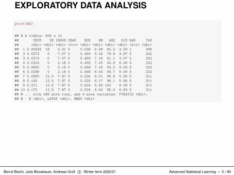
print(bh)
## # A tibble: 506 x 14## CRIM ZN INDUS CHAS NOX RM AGE DIS RAD TAX## <dbl> <dbl> <dbl> <fct> <dbl> <dbl> <dbl> <dbl> <fct> <dbl>## 1 0.00632 18 2.31 0 0.538 6.58 65.2 4.09 1 296## 2 0.0273 0 7.07 0 0.469 6.42 78.9 4.97 2 242## 3 0.0273 0 7.07 0 0.469 7.18 61.1 4.97 2 242## 4 0.0324 0 2.18 0 0.458 7.00 45.8 6.06 3 222## 5 0.0690 0 2.18 0 0.458 7.15 54.2 6.06 3 222## 6 0.0298 0 2.18 0 0.458 6.43 58.7 6.06 3 222## 7 0.0883 12.5 7.87 0 0.524 6.01 66.6 5.56 5 311## 8 0.145 12.5 7.87 0 0.524 6.17 96.1 5.95 5 311## 9 0.211 12.5 7.87 0 0.524 5.63 100 6.08 5 311## 10 0.170 12.5 7.87 0 0.524 6.00 85.9 6.59 5 311## # ... with 496 more rows, and 4 more variables: PTRATIO <dbl>,## # B <dbl>, LSTAT <dbl>, MEDV <dbl>
Bernd Bischl, Julia Moosbauer, Andreas Groll c� Winter term 2020/21 Advanced Statistical Learning – 5 / 99
EXPLORATORY DATA ANALYSISFactor variables
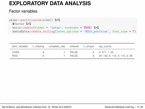
skimr::partition(skim(bh)) %>%.$factor %>%knitr::kable(format = ’latex’, booktabs = TRUE) %>%kableExtra::kable_styling(latex_options = ’HOLD_position’, font_size = 7)
skim_variable n_missing complete_rate ordered n_unique top_counts
CHAS 0 1 FALSE 2 0: 471, 1: 35RAD 0 1 FALSE 9 24: 132, 5: 115, 4: 110, 3: 38
Bernd Bischl, Julia Moosbauer, Andreas Groll c� Winter term 2020/21 Advanced Statistical Learning – 6 / 99

EXPLORATORY DATA ANALYSISBarplots of discrete features
DataExplorer::plot_bar(bh, ggtheme = ggpubr::theme_pubr())
CHAS RAD
0 100 200 300 400 0 50 1007128634524
1
0
Frequency
Bernd Bischl, Julia Moosbauer, Andreas Groll c� Winter term 2020/21 Advanced Statistical Learning – 7 / 99

EXPLORATORY DATA ANALYSISNumeric variables
skimr::partition(skim(bh)) %>%.$numeric %>%dplyr::select(skim_variable, n_missing, mean, sd) %>%knitr::kable(format = ’latex’, booktabs = TRUE) %>%kableExtra::kable_styling(latex_options = ’HOLD_position’, font_size = 6)
skim_variable n_missing mean sd
CRIM 0 3.614 8.602ZN 0 11.364 23.322INDUS 0 11.137 6.860NOX 0 0.555 0.116RM 0 6.285 0.703
AGE 0 68.575 28.149DIS 0 3.795 2.106TAX 0 408.237 168.537PTRATIO 0 18.456 2.165B 0 356.674 91.295
LSTAT 0 12.653 7.141MEDV 0 22.533 9.197
Bernd Bischl, Julia Moosbauer, Andreas Groll c� Winter term 2020/21 Advanced Statistical Learning – 8 / 99

EXPLORATORY DATA ANALYSISHistograms of numerical features
DataExplorer::plot_histogram(bh, ggtheme = ggpubr::theme_pubr())
PTRATIO RM TAX ZN
INDUS LSTAT MEDV NOX
AGE B CRIM DIS
12.515.017.520.022.5 4 5 6 7 8 9 200300400500600700 0 25 50 75 100
0 10 20 0 10 20 30 10 20 30 40 50 0.4 0.5 0.6 0.7 0.8 0.9
0 25 50 75 100 0 100 200 300 400 0 25 50 75 2.5 5.0 7.510.012.50204060
02040
0100200300
0100200300
0204060
050100
0100200
01020304050
020406080
01020304050
050100
050100150
value
Frequency
Bernd Bischl, Julia Moosbauer, Andreas Groll c� Winter term 2020/21 Advanced Statistical Learning – 9 / 99

EXPLORATORY DATA ANALYSISIt is always useful to check the correlation among variables:
DataExplorer::plot_correlation(bh, ggtheme = ggpubr::theme_pubr(base_size = 10),type = "c", cor_args = list(use = "complete.obs"))
1 −0.2 0.41 0.42 −0.22 0.35 −0.38 0.58 0.29 −0.39 0.46 −0.39−0.2 1 −0.53 −0.52 0.31 −0.57 0.66 −0.31 −0.39 0.18 −0.41 0.360.41 −0.53 1 0.76 −0.39 0.64 −0.71 0.72 0.38 −0.36 0.6 −0.480.42 −0.52 0.76 1 −0.3 0.73 −0.77 0.67 0.19 −0.38 0.59 −0.43−0.22 0.31 −0.39 −0.3 1 −0.24 0.21 −0.29 −0.36 0.13 −0.61 0.70.35 −0.57 0.64 0.73 −0.24 1 −0.75 0.51 0.26 −0.27 0.6 −0.38−0.38 0.66 −0.71 −0.77 0.21 −0.75 1 −0.53 −0.23 0.29 −0.5 0.250.58 −0.31 0.72 0.67 −0.29 0.51 −0.53 1 0.46 −0.44 0.54 −0.470.29 −0.39 0.38 0.19 −0.36 0.26 −0.23 0.46 1 −0.18 0.37 −0.51−0.39 0.18 −0.36 −0.38 0.13 −0.27 0.29 −0.44 −0.18 1 −0.37 0.330.46 −0.41 0.6 0.59 −0.61 0.6 −0.5 0.54 0.37 −0.37 1 −0.74−0.39 0.36 −0.48 −0.43 0.7 −0.38 0.25 −0.47 −0.51 0.33 −0.74 1
CRIMZN
INDUSNOXRM
AGEDISTAX
PTRATIOB
LSTATMEDV
CRIM
ZN
INDU
S
NOX
RM AGE
DIS
TAX
PTRA
TIO
B
LSTA
T
MED
V
Features
Feat
ures
−1.0 −0.5 0.0 0.5 1.0Correlation Meter
Bernd Bischl, Julia Moosbauer, Andreas Groll c� Winter term 2020/21 Advanced Statistical Learning – 10 / 99

Credit Data Set
Bernd Bischl, Julia Moosbauer, Andreas Groll c� Winter term 2020/21 Advanced Statistical Learning – 11 / 99

CREDIT DATA SET
German Credit Dataset is a research dataset from the University ofHamburg from 1994 and donated by Prof. Hans Hoffman.
Each entry represents a person who takes a credit by a bank.Each person is classified as "good" or "bad" credit risks accordingto the set of attributes.
Bernd Bischl, Julia Moosbauer, Andreas Groll c� Winter term 2020/21 Advanced Statistical Learning – 12 / 99

CREDIT DATA SETVariable Descriptionclass "good" | "bad"checking_status Status of existing checking accountduration Duration in monthcredit_history Credit historycredit_amount Amount of the desired creditsaving_status Amount in savings accountemployment Present employment since, in yearsinstallment_commitment Installment rate in percentage of disposable incomepersonal_status Personal status and sexother_parties Other debtors or guarantorsresidence_since Current residence since, in yearsage Age in yearsother_payment_plans Other installment plansexisting_credits Number of existing credits at this bankjob Current jobnum_dependents Number of people being liable to provide maintenance forown_telephone Telephone (yes|no)foreign_worker foreign worker (yes|no)
1000 obs., 21 features, class binary target.
Bernd Bischl, Julia Moosbauer, Andreas Groll c� Winter term 2020/21 Advanced Statistical Learning – 13 / 99

IMPORTING THE DATA
We use OpenML (R-Package) to download the dataset in amachine-readable format and convert it into a data.frame:
# load the dataset from OpenML Library
d = OpenML::getOMLDataSet(data.id = 31)
# convert the OpenML object to a tibble (enhanced data.frame)
credit = tibble::as_tibble(d)
Bernd Bischl, Julia Moosbauer, Andreas Groll c� Winter term 2020/21 Advanced Statistical Learning – 14 / 99

EXPLORATORY DATA ANALYSIS
print(head(credit))
## # A tibble: 6 x 21## checking_status duration credit_history purpose credit_amount savings_status employment## <fct> <dbl> <fct> <fct> <dbl> <fct> <fct>## 1 <0 6 critical/othe~ radio/~ 1169 no known savi~ >=7## 2 0<=X<200 48 existing paid radio/~ 5951 <100 1<=X<4## 3 no checking 12 critical/othe~ educat~ 2096 <100 4<=X<7## 4 <0 42 existing paid furnit~ 7882 <100 4<=X<7## 5 <0 24 delayed previ~ new car 4870 <100 1<=X<4## 6 no checking 36 existing paid educat~ 9055 no known savi~ 1<=X<4## # ... with 14 more variables: installment_commitment <dbl>, personal_status <fct>,## # other_parties <fct>, residence_since <dbl>, property_magnitude <fct>, age <dbl>,## # other_payment_plans <fct>, housing <fct>, existing_credits <dbl>, job <fct>,## # num_dependents <dbl>, own_telephone <fct>, foreign_worker <fct>, class <fct>
Bernd Bischl, Julia Moosbauer, Andreas Groll c� Winter term 2020/21 Advanced Statistical Learning – 15 / 99

EXPLORATORY DATA ANALYSISFactor Variables
skimr::partition(skim(credit)) %>%.$factor %>%knitr::kable(format = ’latex’, booktabs = TRUE) %>%kableExtra::kable_styling(latex_options = ’HOLD_position’, font_size = 5)
skim_variable n_missing complete_rate ordered n_unique top_counts
checking_status 0 1 FALSE 4 no : 394, <0: 274, 0<=: 269, >=2: 63credit_history 0 1 FALSE 5 exi: 530, cri: 293, del: 88, all: 49purpose 0 1 FALSE 10 rad: 280, new: 234, fur: 181, use: 103savings_status 0 1 FALSE 5 <10: 603, no : 183, 100: 103, 500: 63employment 0 1 FALSE 5 1<=: 339, >=7: 253, 4<=: 174, <1: 172
personal_status 0 1 FALSE 4 mal: 548, fem: 310, mal: 92, mal: 50other_parties 0 1 FALSE 3 non: 907, gua: 52, co : 41property_magnitude 0 1 FALSE 4 car: 332, rea: 282, lif: 232, no : 154other_payment_plans 0 1 FALSE 3 non: 814, ban: 139, sto: 47housing 0 1 FALSE 3 own: 713, ren: 179, for: 108
job 0 1 FALSE 4 ski: 630, uns: 200, hig: 148, une: 22own_telephone 0 1 FALSE 2 non: 596, yes: 404foreign_worker 0 1 FALSE 2 yes: 963, no: 37class 0 1 FALSE 2 goo: 700, bad: 300
Bernd Bischl, Julia Moosbauer, Andreas Groll c� Winter term 2020/21 Advanced Statistical Learning – 16 / 99

EXPLORATORY DATA ANALYSISBarplots of discrete features
plot_bar(credit[, 1:14], ggtheme = ggpubr::theme_pubr(base_size = 7.5))
other_parties property_magnitude other_payment_plans
savings_status employment personal_status
checking_status credit_history purpose
0 250 500 750 0 100 200 300 0 200 400 600 800
0 200 400 600 0 100 200 300 0 200 400
0 100 200 300 400 0 200 400 0 100 200retraining
domestic applianceother
repairseducationbusinessused car
furniture/equipmentnew carradio/tv
male div/sep
male mar/wid
female div/dep/mar
male single
stores
bank
none
no credits/all paidall paid
delayed previouslycritical/other existing credit
existing paid
unemployed<1
4<=X<7>=7
1<=X<4
no known property
life insurance
real estate
car
>=200
0<=X<200
<0
no checking
>=1000500<=X<1000
100<=X<500no known savings
<100
co applicant
guarantor
none
Frequency
Bernd Bischl, Julia Moosbauer, Andreas Groll c� Winter term 2020/21 Advanced Statistical Learning – 17 / 99

EXPLORATORY DATA ANALYSISBarplots of discrete features
plot_bar(credit[, 15:21], ggtheme = ggpubr::theme_pubr(base_size = 9))
foreign_worker class num_dependents
housing job own_telephone
0 250 500 750 1000 0 200 400 600 0 200 400 600 800
0 200 400 600 0 200 400 600 0 200 400 600
yes
none
2
1
unemp/unskilled non res
high qualif/self emp/mgmt
unskilled resident
skilled
bad
good
for free
rent
own
no
yes
Frequency
Bernd Bischl, Julia Moosbauer, Andreas Groll c� Winter term 2020/21 Advanced Statistical Learning – 18 / 99

EXPLORATORY DATA ANALYSISNumerical Variables
skimr::partition(skim(credit)) %>%.$numeric %>%dplyr::select(skim_variable, n_missing, mean, sd) %>%knitr::kable(format = ’latex’, booktabs = TRUE)
skim_variable n_missing mean sd
duration 0 20.90 12.059credit_amount 0 3271.26 2822.737installment_commitment 0 2.97 1.119residence_since 0 2.85 1.104age 0 35.55 11.375
existing_credits 0 1.41 0.578num_dependents 0 1.16 0.362
Bernd Bischl, Julia Moosbauer, Andreas Groll c� Winter term 2020/21 Advanced Statistical Learning – 19 / 99

EXPLORATORY DATA ANALYSISHistograms of numerical features
plot_histogram(credit, ggtheme = ggpubr::theme_pubr())
installment_commitment residence_since
age credit_amount duration existing_credits
1 2 3 4 1 2 3 4
20 40 60 0 50001000015000 0 20 40 60 1 2 3 40
200
400
600
050100150
050100150200
0100200300400
0255075
0100200300400
value
Frequency
Bernd Bischl, Julia Moosbauer, Andreas Groll c� Winter term 2020/21 Advanced Statistical Learning – 20 / 99

EXPLORATORY DATA ANALYSISIt is always useful to check the correlation among variables:
DataExplorer::plot_correlation(credit, ggtheme = ggpubr::theme_pubr(base_size = 10),type = "c", cor_args = list(use = "complete.obs"))
1 0.62 0.07 0.03 −0.04 −0.01 −0.020.62 1 −0.27 0.03 0.03 0.02 0.020.07 −0.27 1 0.05 0.06 0.02 −0.070.03 0.03 0.05 1 0.27 0.09 0.04−0.04 0.03 0.06 0.27 1 0.15 0.12−0.01 0.02 0.02 0.09 0.15 1 0.11−0.02 0.02 −0.07 0.04 0.12 0.11 1
durationcredit_amount
installment_commitmentresidence_since
ageexisting_credits
num_dependents
dura
tion
cred
it_am
ount
inst
allm
ent_
com
mitm
ent
resi
denc
e_si
nce
age
exis
ting_
cred
its
num
_dep
ende
nts
Features
Feat
ures
−1.0 −0.5 0.0 0.5 1.0Correlation Meter
Bernd Bischl, Julia Moosbauer, Andreas Groll c� Winter term 2020/21 Advanced Statistical Learning – 21 / 99

Iris Data Set
Bernd Bischl, Julia Moosbauer, Andreas Groll c� Winter term 2020/21 Advanced Statistical Learning – 22 / 99

IRIS DATA SET
The iris dataset was introduced by the statistician Ronald Fisher and isone of the most frequent used datasets. Originally it was designed forlinear discriminant analysis.The set is a typical test case for many statistical classificationtechniques and has its own wikipedia page.
Setosa Versicolor Virginica
Source: https://en.wikipedia.org/wiki/Iris_flower_data_set
Bernd Bischl, Julia Moosbauer, Andreas Groll c� Winter term 2020/21 Advanced Statistical Learning – 23 / 99

IMPORTING THE DATA
We use OpenML (R-Package) to download the dataset in amachine-readable format and convert it into a data.frame:
# load the dataset from OpenML Library
d = OpenML::getOMLDataSet(data.id = 61)
# convert the OpenML object to a tibble (enhanced data.frame)
iris = tibble::as_tibble(d)
Bernd Bischl, Julia Moosbauer, Andreas Groll c� Winter term 2020/21 Advanced Statistical Learning – 24 / 99

IMPORTING THE DATA150 iris flowers (50 setosa, 50 versicolor, 50 virginica), speciesshould be predicted.
Sepal length / width and petal length / width in [cm].
Source: https://holgerbrandl.github.io/kotlin4ds_kotlin_night_frankfurt//krangl_example_report.html
Bernd Bischl, Julia Moosbauer, Andreas Groll c� Winter term 2020/21 Advanced Statistical Learning – 25 / 99

IMPORTING THE DATAprint(iris)
## # A tibble: 150 x 5## sepallength sepalwidth petallength petalwidth class## <dbl> <dbl> <dbl> <dbl> <fct>## 1 5.1 3.5 1.4 0.2 Iris-setosa## 2 4.9 3 1.4 0.2 Iris-setosa## 3 4.7 3.2 1.3 0.2 Iris-setosa## 4 4.6 3.1 1.5 0.2 Iris-setosa## 5 5 3.6 1.4 0.2 Iris-setosa## 6 5.4 3.9 1.7 0.4 Iris-setosa## 7 4.6 3.4 1.4 0.3 Iris-setosa## 8 5 3.4 1.5 0.2 Iris-setosa## 9 4.4 2.9 1.4 0.2 Iris-setosa## 10 4.9 3.1 1.5 0.1 Iris-setosa## # ... with 140 more rows
Bernd Bischl, Julia Moosbauer, Andreas Groll c� Winter term 2020/21 Advanced Statistical Learning – 26 / 99

EXPLORATORY DATA ANALYSIS
Factor variables
skimr::partition(skim(iris)) %>%.$factor %>%knitr::kable(format = ’latex’, booktabs = TRUE) %>%kableExtra::kable_styling(latex_options = ’HOLD_position’, font_size = 7)
skim_variable n_missing complete_rate ordered n_unique top_counts
class 0 1 FALSE 3 Iri: 50, Iri: 50, Iri: 50
Bernd Bischl, Julia Moosbauer, Andreas Groll c� Winter term 2020/21 Advanced Statistical Learning – 27 / 99

EXPLORATORY DATA ANALYSISBarplots of discrete features
DataExplorer::plot_bar(iris, ggtheme = ggpubr::theme_pubr())
class
0 10 20 30 40 50
Iris−setosa
Iris−versicolor
Iris−virginica
Frequency
Bernd Bischl, Julia Moosbauer, Andreas Groll c� Winter term 2020/21 Advanced Statistical Learning – 28 / 99

EXPLORATORY DATA ANALYSISNumeric variables
skimr::partition(skim(iris)) %>%.$numeric %>%dplyr::select(skim_variable, n_missing, mean, sd) %>%knitr::kable(format = ’latex’, booktabs = TRUE) %>%kableExtra::kable_styling(latex_options = ’HOLD_position’, font_size = 8)
skim_variable n_missing mean sd
sepallength 0 5.84 0.828sepalwidth 0 3.05 0.434petallength 0 3.76 1.764petalwidth 0 1.20 0.763
Bernd Bischl, Julia Moosbauer, Andreas Groll c� Winter term 2020/21 Advanced Statistical Learning – 29 / 99

EXPLORATORY DATA ANALYSISHistograms of numerical features
DataExplorer::plot_histogram(iris, ggtheme = ggpubr::theme_pubr())
petallength petalwidth sepallength sepalwidth
2 4 6 0.0 0.5 1.0 1.5 2.0 2.5 5 6 7 8 2.0 2.5 3.0 3.5 4.0 4.5
0
10
20
0.0
2.5
5.0
7.5
10.0
12.5
0
10
20
0
10
20
value
Frequency
Bernd Bischl, Julia Moosbauer, Andreas Groll c� Winter term 2020/21 Advanced Statistical Learning – 30 / 99

Ozone Data Set
Bernd Bischl, Julia Moosbauer, Andreas Groll c� Winter term 2020/21 Advanced Statistical Learning – 31 / 99

OZONE DATA SET
All measurements were taken in the area of Upland, CA, east ofLos Angeles.
The aim is to predict the daily maximum one-hour-average ozonereading (V4).
Introduced in Breiman, L. and Friedman, J. (1985), "EstimatingOptimal Transformations for Multiple Regression and Correlation",Journal of the American Statistical Association, 80, 580-598.
Bernd Bischl, Julia Moosbauer, Andreas Groll c� Winter term 2020/21 Advanced Statistical Learning – 32 / 99

IMPORTING THE DATA
We load the data from the mlbench package:
library(mlbench)data(Ozone)
# convert the OpenML object to a tibble (enhanced data.frame)
ozone = tibble::as_tibble(Ozone)
The variables are: elevation, temperature (surface and air), ozone, airpressure, and cloud cover (low, mid, and high).
Bernd Bischl, Julia Moosbauer, Andreas Groll c� Winter term 2020/21 Advanced Statistical Learning – 33 / 99
EXPLORATORY DATA ANALYSIS
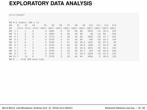
print(ozone)
## # A tibble: 366 x 13## V1 V2 V3 V4 V5 V6 V7 V8 V9 V10 V11 V12 V13## <fct> <fct> <fct> <dbl> <dbl> <dbl> <dbl> <dbl> <dbl> <dbl> <dbl> <dbl> <dbl>## 1 1 1 4 3 5480 8 20 NA NA 5000 -15 30.6 200## 2 1 2 5 3 5660 6 NA 38 NA NA -14 NA 300## 3 1 3 6 3 5710 4 28 40 NA 2693 -25 47.7 250## 4 1 4 7 5 5700 3 37 45 NA 590 -24 55.0 100## 5 1 5 1 5 5760 3 51 54 45.3 1450 25 57.0 60## 6 1 6 2 6 5720 4 69 35 49.6 1568 15 53.8 60## 7 1 7 3 4 5790 6 19 45 46.4 2631 -33 54.1 100## 8 1 8 4 4 5790 3 25 55 52.7 554 -28 64.8 250## 9 1 9 5 6 5700 3 73 41 48.0 2083 23 52.5 120## 10 1 10 6 7 5700 3 59 44 NA 2654 -2 48.4 120## # ... with 356 more rows
Bernd Bischl, Julia Moosbauer, Andreas Groll c� Winter term 2020/21 Advanced Statistical Learning – 34 / 99

EXPLORATORY DATA ANALYSISVariable DescriptionV1 Month: 1 = January, ..., 12 = DecemberV2 Day of monthV3 Day of week: 1 = Monday, ..., 7 = SundayV4 Daily maximum one-hour-average ozone readingV5 500 millibar pressure height (m) measured at Vandenberg AFBV6 Wind speed (mph) at Los Angeles International Airport (LAX)V7 Humidity (%) at LAXV8 Temperature (degrees F) measured at Sandburg, CAV9 Temperature (degrees F) measured at El Monte, CAV10 Inversion base height (feet) at LAXV11 Pressure gradient (mm Hg) from LAX to Daggett, CAV12 Inversion base temperature (degrees F) at LAXV13 Visibility (miles) measured at LAX
366 obs., 13 features, V4 numeric target.
Bernd Bischl, Julia Moosbauer, Andreas Groll c� Winter term 2020/21 Advanced Statistical Learning – 35 / 99

EXPLORATORY DATA ANALYSISFactor Variables
skimr::partition(skim(ozone)) %>%.$factor %>%knitr::kable(format = ’latex’, booktabs = TRUE) %>%kableExtra::kable_styling(latex_options = ’HOLD_position’, font_size = 7)
skim_variable n_missing complete_rate ordered n_unique top_counts
V1 0 1 FALSE 12 1: 31, 3: 31, 5: 31, 7: 31V2 0 1 FALSE 31 1: 12, 2: 12, 3: 12, 4: 12V3 0 1 FALSE 7 4: 53, 5: 53, 1: 52, 2: 52
Bernd Bischl, Julia Moosbauer, Andreas Groll c� Winter term 2020/21 Advanced Statistical Learning – 36 / 99

EXPLORATORY DATA ANALYSISNumerical Variables
skimr::partition(skim(ozone)) %>%.$numeric %>%dplyr::select(skim_variable, n_missing, mean, sd) %>%knitr::kable(format = ’latex’, booktabs = TRUE) %>%kableExtra::kable_styling(latex_options = ’HOLD_position’, font_size = 7)
skim_variable n_missing mean sd
V4 5 11.53 7.92V5 12 5752.97 104.99V6 0 4.87 2.12V7 15 58.48 19.76V8 2 61.91 14.28
V9 139 56.85 11.66V10 15 2590.94 1796.83V11 1 17.80 36.11V12 14 60.93 13.87V13 0 123.30 80.28
Bernd Bischl, Julia Moosbauer, Andreas Groll c� Winter term 2020/21 Advanced Statistical Learning – 37 / 99
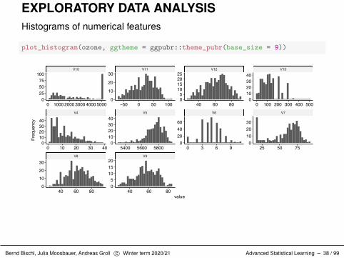
EXPLORATORY DATA ANALYSISHistograms of numerical features
plot_histogram(ozone, ggtheme = ggpubr::theme_pubr(base_size = 9))
V8 V9
V4 V5 V6 V7
V10 V11 V12 V13
40 60 80 40 60 80
0 10 20 30 40 5400 5600 5800 0 3 6 9 25 50 75
0 1000 2000 3000 4000 5000 −50 0 50 100 40 60 80 0 100 200 300 400 500010203040
0102030
0510152025
0204060
0
10
20
30
010203040
05101520
0255075100
010203040
0
10
20
30
value
Frequency
Bernd Bischl, Julia Moosbauer, Andreas Groll c� Winter term 2020/21 Advanced Statistical Learning – 38 / 99

EXPLORATORY DATA ANALYSISIt seems that we have quite some missing observations. Let’s take acloser look:
DataExplorer::plot_missing(ozone, ggtheme = ggpubr::theme_pubr())
0%0%0%
1.37%3.28%
0%
4.1%
0.55%
37.98%
4.1%
0.27%
3.83%
0%
V9V7
V10V12V5V4V8
V11V1V2V3V6
V13
0 50 100Missing Rows
Feat
ures
Band Good OK
Bernd Bischl, Julia Moosbauer, Andreas Groll c� Winter term 2020/21 Advanced Statistical Learning – 39 / 99
PID Data Set
Bernd Bischl, Julia Moosbauer, Andreas Groll c� Winter term 2020/21 Advanced Statistical Learning – 40 / 99
PID DATA SET
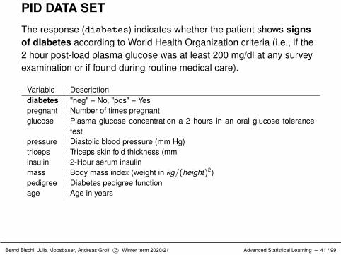
The response (diabetes) indicates whether the patient shows signsof diabetes according to World Health Organization criteria (i.e., if the2 hour post-load plasma glucose was at least 200 mg/dl at any surveyexamination or if found during routine medical care).
Variable Descriptiondiabetes "neg" = No, "pos" = Yespregnant Number of times pregnantglucose Plasma glucose concentration a 2 hours in an oral glucose tolerance
testpressure Diastolic blood pressure (mm Hg)triceps Triceps skin fold thickness (mminsulin 2-Hour serum insulinmass Body mass index (weight in kg/(height)2)pedigree Diabetes pedigree functionage Age in years
Bernd Bischl, Julia Moosbauer, Andreas Groll c� Winter term 2020/21 Advanced Statistical Learning – 41 / 99

Sonar Data Set
Bernd Bischl, Julia Moosbauer, Andreas Groll c� Winter term 2020/21 Advanced Statistical Learning – 42 / 99

SONAR DATA SET
This is the data set used by Gorman and Sejnowski in their study("Analysis of Hidden Units in a Layered Network Trained to ClassifySonar Targets" in Neural Networks, Vol. 1, pp. 75-89.) of theclassification of sonar signals using a neural network. The task is totrain a network to discriminate between sonar signals bounced off ametal cylinder and those bounced off a roughly cylindrical rock.
attribute_[1-60]: Each variable represents the energy withina particular frequency band, integrated over a certain period oftime. The integration aperture for higher frequencies occur later intime, since these frequencies are transmitted later during the chirp.
class: "Rock" / "Mine (metal cylinder)"
The numbers in the labels are in increasing order of aspect angle, butthey do not encode the angle directly.
Bernd Bischl, Julia Moosbauer, Andreas Groll c� Winter term 2020/21 Advanced Statistical Learning – 43 / 99

IMPORTING THE DATA
We use OpenML (R-Package) to download the dataset in amachine-readable format and convert it into a data.frame:
# load the dataset from OpenML Library
d = OpenML::getOMLDataSet(data.id = 40)
# convert the OpenML object to a tibble (enhanced data.frame)
sonar = tibble::as_tibble(d)
Bernd Bischl, Julia Moosbauer, Andreas Groll c� Winter term 2020/21 Advanced Statistical Learning – 44 / 99

EXPLORATORY DATA ANALYSIS
print(head(sonar, n = 2L))
## # A tibble: 2 x 61## attribute_1 attribute_2 attribute_3 attribute_4 attribute_5 attribute_6 attribute_7## <dbl> <dbl> <dbl> <dbl> <dbl> <dbl> <dbl>## 1 0.02 0.0371 0.0428 0.0207 0.0954 0.0986 0.154## 2 0.0453 0.0523 0.0843 0.0689 0.118 0.258 0.216## # ... with 54 more variables: attribute_8 <dbl>, attribute_9 <dbl>, attribute_10 <dbl>,## # attribute_11 <dbl>, attribute_12 <dbl>, attribute_13 <dbl>, attribute_14 <dbl>,## # attribute_15 <dbl>, attribute_16 <dbl>, attribute_17 <dbl>, attribute_18 <dbl>,## # attribute_19 <dbl>, attribute_20 <dbl>, attribute_21 <dbl>, attribute_22 <dbl>,## # attribute_23 <dbl>, attribute_24 <dbl>, attribute_25 <dbl>, attribute_26 <dbl>,## # attribute_27 <dbl>, attribute_28 <dbl>, attribute_29 <dbl>, attribute_30 <dbl>,## # attribute_31 <dbl>, attribute_32 <dbl>, attribute_33 <dbl>, attribute_34 <dbl>,## # attribute_35 <dbl>, attribute_36 <dbl>, attribute_37 <dbl>, attribute_38 <dbl>,## # attribute_39 <dbl>, attribute_40 <dbl>, attribute_41 <dbl>, attribute_42 <dbl>,## # attribute_43 <dbl>, attribute_44 <dbl>, attribute_45 <dbl>, attribute_46 <dbl>,## # attribute_47 <dbl>, attribute_48 <dbl>, attribute_49 <dbl>, attribute_50 <dbl>,## # attribute_51 <dbl>, attribute_52 <dbl>, attribute_53 <dbl>, attribute_54 <dbl>,## # attribute_55 <dbl>, attribute_56 <dbl>, attribute_57 <dbl>, attribute_58 <dbl>,## # attribute_59 <dbl>, attribute_60 <dbl>, Class <fct>
Bernd Bischl, Julia Moosbauer, Andreas Groll c� Winter term 2020/21 Advanced Statistical Learning – 45 / 99
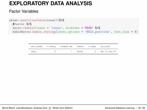
EXPLORATORY DATA ANALYSISFactor Variables
skimr::partition(skim(sonar))%>%.$factor %>%knitr::kable(format = ’latex’, booktabs = TRUE) %>%kableExtra::kable_styling(latex_options = ’HOLD_position’, font_size = 5)
skim_variable n_missing complete_rate ordered n_unique top_counts
Class 0 1 FALSE 2 Min: 111, Roc: 97
Bernd Bischl, Julia Moosbauer, Andreas Groll c� Winter term 2020/21 Advanced Statistical Learning – 46 / 99

EXPLORATORY DATA ANALYSISBarplots of discrete features
plot_bar(sonar, ggtheme = ggpubr::theme_pubr(base_size = 7))
Class
0 30 60 90
Rock
Mine
Frequency
Bernd Bischl, Julia Moosbauer, Andreas Groll c� Winter term 2020/21 Advanced Statistical Learning – 47 / 99

EXPLORATORY DATA ANALYSISNumerical Variables
skimr::partition(skim(sonar[, 1:15])) %>%.$numeric %>%dplyr::select(skim_variable, n_missing, mean, sd) %>%knitr::kable(format = ’latex’, booktabs = TRUE) %>%kableExtra::kable_styling(latex_options = ’HOLD_position’, font_size = 4)
skim_variable n_missing mean sd
attribute_1 0 0.029 0.023
attribute_2 0 0.038 0.033
attribute_3 0 0.044 0.038
attribute_4 0 0.054 0.047
attribute_5 0 0.075 0.056
attribute_6 0 0.105 0.059
attribute_7 0 0.122 0.062
attribute_8 0 0.135 0.085
attribute_9 0 0.178 0.118
attribute_10 0 0.208 0.134
attribute_11 0 0.236 0.133
attribute_12 0 0.250 0.140
attribute_13 0 0.273 0.141
attribute_14 0 0.297 0.164
attribute_15 0 0.320 0.205
Bernd Bischl, Julia Moosbauer, Andreas Groll c� Winter term 2020/21 Advanced Statistical Learning – 48 / 99

EXPLORATORY DATA ANALYSISHistograms of numerical features
plot_histogram(sonar[, 1:16], ggtheme = ggpubr::theme_pubr(base_size = 7))
attribute_6 attribute_7 attribute_8 attribute_9
attribute_2 attribute_3 attribute_4 attribute_5
attribute_13 attribute_14 attribute_15 attribute_16
attribute_1 attribute_10 attribute_11 attribute_12
0.0 0.1 0.2 0.3 0.4 0.0 0.1 0.2 0.3 0.0 0.1 0.2 0.3 0.4 0.0 0.2 0.4 0.6
0.00 0.05 0.10 0.15 0.20 0.0 0.1 0.2 0.3 0.0 0.1 0.2 0.3 0.4 0.0 0.1 0.2 0.3 0.4
0.0 0.2 0.4 0.6 0.00 0.25 0.50 0.75 1.00 0.00 0.25 0.50 0.75 1.00 0.00 0.25 0.50 0.75 1.00
0.00 0.05 0.10 0.0 0.2 0.4 0.6 0.0 0.2 0.4 0.6 0.0 0.2 0.4 0.605101520
05101520
0102030
05101520
05101520
0510152025
010203040
0
10
20
05101520
0
10
20
0102030
0
10
20
0
10
20
30
051015
0102030
0
10
20
30
value
Frequency
Bernd Bischl, Julia Moosbauer, Andreas Groll c� Winter term 2020/21 Advanced Statistical Learning – 49 / 99

EXPLORATORY DATA ANALYSISHistograms of numerical features
plot_histogram(sonar[, 17:32], ggtheme = ggpubr::theme_pubr(base_size = 7))
attribute_29 attribute_30 attribute_31 attribute_32
attribute_25 attribute_26 attribute_27 attribute_28
attribute_21 attribute_22 attribute_23 attribute_24
attribute_17 attribute_18 attribute_19 attribute_20
0.00 0.25 0.50 0.75 1.00 0.00 0.25 0.50 0.75 1.00 0.00 0.25 0.50 0.75 1.00 0.00 0.25 0.50 0.75
0.00 0.25 0.50 0.75 1.00 0.25 0.50 0.75 1.00 0.00 0.25 0.50 0.75 1.00 0.00 0.25 0.50 0.75 1.00
0.00 0.25 0.50 0.75 1.00 0.00 0.25 0.50 0.75 1.00 0.00 0.25 0.50 0.75 1.00 0.00 0.25 0.50 0.75 1.00
0.00 0.25 0.50 0.75 1.00 0.00 0.25 0.50 0.75 1.00 0.00 0.25 0.50 0.75 1.00 0.25 0.50 0.75 1.000
5
10
0
5
10
15
051015
0
5
10
15
051015
0
5
10
0
10
20
30
0
5
10
15
05101520
0
5
10
15
0
5
10
15
051015
051015
0
5
10
0
5
10
15
051015
value
Frequency
Bernd Bischl, Julia Moosbauer, Andreas Groll c� Winter term 2020/21 Advanced Statistical Learning – 50 / 99

EXPLORATORY DATA ANALYSISHistograms of numerical features
plot_histogram(sonar[, 33:48], ggtheme = ggpubr::theme_pubr(base_size = 7))
attribute_45 attribute_46 attribute_47 attribute_48
attribute_41 attribute_42 attribute_43 attribute_44
attribute_37 attribute_38 attribute_39 attribute_40
attribute_33 attribute_34 attribute_35 attribute_36
0.0 0.2 0.4 0.6 0.0 0.2 0.4 0.6 0.0 0.2 0.4 0.0 0.1 0.2 0.3
0.00 0.25 0.50 0.75 0.0 0.2 0.4 0.6 0.8 0.0 0.2 0.4 0.6 0.8 0.0 0.2 0.4 0.6 0.8
0.00 0.25 0.50 0.75 1.00 0.00 0.25 0.50 0.75 1.00 0.00 0.25 0.50 0.75 1.00 0.00 0.25 0.50 0.75
0.00 0.25 0.50 0.75 1.00 0.00 0.25 0.50 0.75 1.00 0.00 0.25 0.50 0.75 1.00 0.00 0.25 0.50 0.75 1.00051015
051015
0
10
20
0510152025
0
5
10
15
05101520
0510152025
0
10
20
051015
05101520
05101520
0
10
20
30
05101520
051015
051015
0
10
20
30
value
Frequency
Bernd Bischl, Julia Moosbauer, Andreas Groll c� Winter term 2020/21 Advanced Statistical Learning – 51 / 99

EXPLORATORY DATA ANALYSISHistograms of numerical features
plot_histogram(sonar[, 49:61], ggtheme = ggpubr::theme_pubr(base_size = 7))
attribute_57 attribute_58 attribute_59 attribute_60
attribute_53 attribute_54 attribute_55 attribute_56
attribute_49 attribute_50 attribute_51 attribute_52
0.00 0.01 0.02 0.03 0.00 0.01 0.02 0.03 0.04 0.00 0.01 0.02 0.03 0.00 0.01 0.02 0.03 0.04
0.00 0.01 0.02 0.03 0.04 0.00 0.01 0.02 0.03 0.00 0.01 0.02 0.03 0.04 0.00 0.01 0.02 0.03 0.04
0.00 0.05 0.10 0.15 0.20 0.00 0.02 0.04 0.06 0.08 0.000 0.025 0.050 0.075 0.100 0.00 0.02 0.04 0.060
10
20
30
0
10
20
30
0
10
20
30
40
0
10
20
30
40
0
10
20
30
0
10
20
30
0
5
10
15
20
0
10
20
0
10
20
30
0510152025
0
5
10
15
20
0
10
20
30
value
Frequency
Bernd Bischl, Julia Moosbauer, Andreas Groll c� Winter term 2020/21 Advanced Statistical Learning – 52 / 99

EXPLORATORY DATA ANALYSISLet’s take a look at the correlation among the variables:
DataExplorer::plot_correlation(sonar, ggtheme = ggpubr::theme_pubr(base_size = 7))
attribute_1attribute_2attribute_3attribute_4attribute_5attribute_6attribute_7attribute_8attribute_9attribute_10attribute_11attribute_12attribute_13attribute_14attribute_15attribute_16attribute_17attribute_18attribute_19attribute_20attribute_21attribute_22attribute_23attribute_24attribute_25attribute_26attribute_27attribute_28attribute_29attribute_30attribute_31attribute_32attribute_33attribute_34attribute_35attribute_36attribute_37attribute_38attribute_39attribute_40attribute_41attribute_42attribute_43attribute_44attribute_45attribute_46attribute_47attribute_48attribute_49attribute_50attribute_51attribute_52attribute_53attribute_54attribute_55attribute_56attribute_57attribute_58attribute_59attribute_60Class_MineClass_Rockat
tribu
te_1
attri
bute
_2at
tribu
te_3
attri
bute
_4at
tribu
te_5
attri
bute
_6at
tribu
te_7
attri
bute
_8at
tribu
te_9
attri
bute
_10
attri
bute
_11
attri
bute
_12
attri
bute
_13
attri
bute
_14
attri
bute
_15
attri
bute
_16
attri
bute
_17
attri
bute
_18
attri
bute
_19
attri
bute
_20
attri
bute
_21
attri
bute
_22
attri
bute
_23
attri
bute
_24
attri
bute
_25
attri
bute
_26
attri
bute
_27
attri
bute
_28
attri
bute
_29
attri
bute
_30
attri
bute
_31
attri
bute
_32
attri
bute
_33
attri
bute
_34
attri
bute
_35
attri
bute
_36
attri
bute
_37
attri
bute
_38
attri
bute
_39
attri
bute
_40
attri
bute
_41
attri
bute
_42
attri
bute
_43
attri
bute
_44
attri
bute
_45
attri
bute
_46
attri
bute
_47
attri
bute
_48
attri
bute
_49
attri
bute
_50
attri
bute
_51
attri
bute
_52
attri
bute
_53
attri
bute
_54
attri
bute
_55
attri
bute
_56
attri
bute
_57
attri
bute
_58
attri
bute
_59
attri
bute
_60
Cla
ss_M
ine
Cla
ss_R
ock
Features
Feat
ures
−1.0 −0.5 0.0 0.5 1.0Correlation Meter
Bernd Bischl, Julia Moosbauer, Andreas Groll c� Winter term 2020/21 Advanced Statistical Learning – 53 / 99

Spam Data Set
Bernd Bischl, Julia Moosbauer, Andreas Groll c� Winter term 2020/21 Advanced Statistical Learning – 54 / 99

SPAM DATA SET
A data set collected at Hewlett-Packard Labs, which classifies 4601e-mails as spam or non-spam (variable "class").
The spam dataset is one of the datasets used in The Elements ofStatistical Learning by Trevor Hastie, Robert Tibshirani, and JeromeFriedman.
Besides the option to import it from OpenML it also comes as anexample dataset in the packages ElemStatLearn and kernlab.
Bernd Bischl, Julia Moosbauer, Andreas Groll c� Winter term 2020/21 Advanced Statistical Learning – 55 / 99

SPAM DATA SETclass : 0 = no spam, 1 = spam
word_freq_*: 48 features corresponding to the relative frequencyof a specific word in an e-mail
char_freq_*: 6 features that measures the percentage of asequence of specific characters occurs relative to the total numberof characters
capital_run_length_[average, longest, total]: 3features indicating the average, longest, and sum of uninterruptedsequence of capital letters
Bernd Bischl, Julia Moosbauer, Andreas Groll c� Winter term 2020/21 Advanced Statistical Learning – 56 / 99

IMPORTING THE DATA
We use OpenML (R-Package) to download the dataset in amachine-readable format and convert it into a data.frame:
# load the dataset from OpenML Library
d = OpenML::getOMLDataSet(data.id = 44)
# convert the OpenML object to a tibble (enhanced data.frame)
spam = tibble::as_tibble(d)
Bernd Bischl, Julia Moosbauer, Andreas Groll c� Winter term 2020/21 Advanced Statistical Learning – 57 / 99

EXPLORATORY DATA ANALYSIS
print(head(spam, n = 5L))
## # A tibble: 5 x 58## word_freq_make word_freq_addre~ word_freq_all word_freq_3d word_freq_our word_freq_over## <dbl> <dbl> <dbl> <dbl> <dbl> <dbl>## 1 0 0.64 0.64 0 0.32 0## 2 0.21 0.28 0.5 0 0.14 0.28## 3 0.06 0 0.71 0 1.23 0.19## 4 0 0 0 0 0.63 0## 5 0 0 0 0 0.63 0## # ... with 52 more variables: word_freq_remove <dbl>, word_freq_internet <dbl>,## # word_freq_order <dbl>, word_freq_mail <dbl>, word_freq_receive <dbl>,## # word_freq_will <dbl>, word_freq_people <dbl>, word_freq_report <dbl>,## # word_freq_addresses <dbl>, word_freq_free <dbl>, word_freq_business <dbl>,## # word_freq_email <dbl>, word_freq_you <dbl>, word_freq_credit <dbl>,## # word_freq_your <dbl>, word_freq_font <dbl>, word_freq_000 <dbl>,## # word_freq_money <dbl>, word_freq_hp <dbl>, word_freq_hpl <dbl>,## # word_freq_george <dbl>, word_freq_650 <dbl>, word_freq_lab <dbl>,## # word_freq_labs <dbl>, word_freq_telnet <dbl>, word_freq_857 <dbl>,## # word_freq_data <dbl>, word_freq_415 <dbl>, word_freq_85 <dbl>,## # word_freq_technology <dbl>, word_freq_1999 <dbl>, word_freq_parts <dbl>,## # word_freq_pm <dbl>, word_freq_direct <dbl>, word_freq_cs <dbl>,## # word_freq_meeting <dbl>, word_freq_original <dbl>, word_freq_project <dbl>,## # word_freq_re <dbl>, word_freq_edu <dbl>, word_freq_table <dbl>,## # word_freq_conference <dbl>, char_freq_.3B <dbl>, char_freq_.28 <dbl>,## # char_freq_.5B <dbl>, char_freq_.21 <dbl>, char_freq_.24 <dbl>, char_freq_.23 <dbl>,## # capital_run_length_average <dbl>, capital_run_length_longest <dbl>,## # capital_run_length_total <dbl>, class <fct>
Bernd Bischl, Julia Moosbauer, Andreas Groll c� Winter term 2020/21 Advanced Statistical Learning – 58 / 99

EXPLORATORY DATA ANALYSISFactor variables
skimr::partition(skim(spam)) %>%.$factor %>%knitr::kable(format = ’latex’, booktabs = TRUE) %>%kableExtra::kable_styling(latex_options = ’HOLD_position’, font_size = 7)
skim_variable n_missing complete_rate ordered n_unique top_counts
class 0 1 FALSE 2 0: 2788, 1: 1813
Bernd Bischl, Julia Moosbauer, Andreas Groll c� Winter term 2020/21 Advanced Statistical Learning – 59 / 99

EXPLORATORY DATA ANALYSISBarplots of discrete features
DataExplorer::plot_bar(spam, ggtheme = ggpubr::theme_pubr())
class
0 1000 2000
1
0
Frequency
Bernd Bischl, Julia Moosbauer, Andreas Groll c� Winter term 2020/21 Advanced Statistical Learning – 60 / 99

EXPLORATORY DATA ANALYSISThe distribution of most variables is highly skewed:
DataExplorer::plot_histogram(spam[, 1:16], ggtheme = ggpubr::theme_pubr())
word_freq_receive word_freq_remove word_freq_report word_freq_will
word_freq_order word_freq_our word_freq_over word_freq_people
word_freq_free word_freq_internet word_freq_mail word_freq_make
word_freq_3d word_freq_address word_freq_addresses word_freq_all
0 1 2 0 2 4 6 0.0 2.5 5.0 7.5 10.0 0.0 2.5 5.0 7.5 10.0
0 2 4 0.0 2.5 5.0 7.5 10.0 0 2 4 6 0 2 4
0 5 10 15 20 0 3 6 9 0 5 10 15 0 1 2 3 4
0 10 20 30 40 0 5 10 15 0 1 2 3 4 0 1 2 3 4 50
10002000
0100020003000
01000200030004000
0500100015002000
01000200030004000
0100020003000
0100020003000
01000200030004000
01000200030004000
01000200030004000
0100020003000
01000200030004000
01000200030004000
0100020003000
01000200030004000
01000200030004000
value
Frequency
Bernd Bischl, Julia Moosbauer, Andreas Groll c� Winter term 2020/21 Advanced Statistical Learning – 61 / 99

EXPLORATORY DATA ANALYSISHistograms of numerical features
DataExplorer::plot_histogram(spam[, 17:32], ggtheme = ggpubr::theme_pubr())
word_freq_money word_freq_telnet word_freq_you word_freq_your
word_freq_hp word_freq_hpl word_freq_lab word_freq_labs
word_freq_credit word_freq_email word_freq_font word_freq_george
word_freq_000 word_freq_650 word_freq_857 word_freq_business
0 5 10 0 5 10 0 5 10 15 20 0 3 6 9
0 5 10 15 20 0 5 10 15 0 5 10 15 0 2 4 6
0 5 10 15 0.0 2.5 5.0 7.5 0 5 10 15 0 10 20 30
0 2 4 0.0 2.5 5.0 7.5 0 1 2 3 4 5 0 2 4 60100020003000
01000200030004000
01000200030004000
0500100015002000
01000200030004000
01000200030004000
01000200030004000
050010001500
01000200030004000
0100020003000
01000200030004000
01000200030004000
01000200030004000
01000200030004000
0100020003000
01000200030004000
value
Frequency
Bernd Bischl, Julia Moosbauer, Andreas Groll c� Winter term 2020/21 Advanced Statistical Learning – 62 / 99

EXPLORATORY DATA ANALYSISHistograms of numerical features
DataExplorer::plot_histogram(spam[, 33:48], ggtheme = ggpubr::theme_pubr())
word_freq_project word_freq_re word_freq_table word_freq_technology
word_freq_meeting word_freq_original word_freq_parts word_freq_pm
word_freq_cs word_freq_data word_freq_direct word_freq_edu
word_freq_1999 word_freq_415 word_freq_85 word_freq_conference
0 5 10 15 20 0 5 10 15 20 0.0 0.5 1.0 1.5 2.0 0 2 4 6 8
0 5 10 15 0 1 2 3 0 2 4 6 8 0 3 6 9
0 2 4 6 0 5 10 15 0 1 2 3 4 5 0 5 10 15 20
0 2 4 6 0 1 2 3 4 5 0 5 10 15 20 0.0 2.5 5.0 7.5 10.001000200030004000
01000200030004000
01000200030004000
01000200030004000
01000200030004000
01000200030004000
01000200030004000
01000200030004000
01000200030004000
01000200030004000
01000200030004000
0100020003000
01000200030004000
01000200030004000
01000200030004000
01000200030004000
value
Frequency
Bernd Bischl, Julia Moosbauer, Andreas Groll c� Winter term 2020/21 Advanced Statistical Learning – 63 / 99
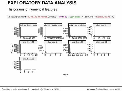
EXPLORATORY DATA ANALYSISHistograms of numerical features
DataExplorer::plot_histogram(spam[, 49:58], ggtheme = ggpubr::theme_pubr())
char_freq_.5B
char_freq_.23 char_freq_.24 char_freq_.28 char_freq_.3B
capital_run_length_average capital_run_length_longest capital_run_length_total char_freq_.21
0 1 2 3 4
0 5 10 15 20 0 2 4 6 0.0 2.5 5.0 7.5 10.0 0 1 2 3 4
0 300 600 900 0 25005000750010000 0 50001000015000 0 10 20 300
1000200030004000
01000200030004000
0100020003000
0100020003000
01000200030004000
0100020003000
01000200030004000
01000200030004000
01000200030004000
value
Frequency
Bernd Bischl, Julia Moosbauer, Andreas Groll c� Winter term 2020/21 Advanced Statistical Learning – 64 / 99
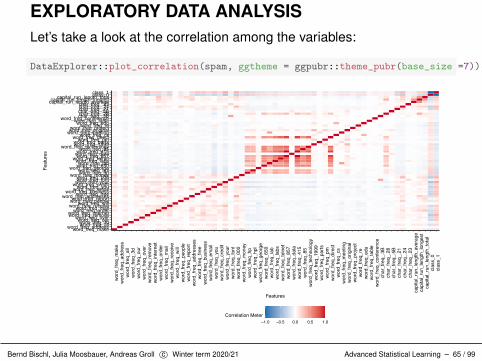
EXPLORATORY DATA ANALYSISLet’s take a look at the correlation among the variables:
DataExplorer::plot_correlation(spam, ggtheme = ggpubr::theme_pubr(base_size =7))
word_freq_makeword_freq_addressword_freq_allword_freq_3dword_freq_ourword_freq_overword_freq_removeword_freq_internetword_freq_orderword_freq_mailword_freq_receiveword_freq_willword_freq_peopleword_freq_reportword_freq_addressesword_freq_freeword_freq_businessword_freq_emailword_freq_youword_freq_creditword_freq_yourword_freq_fontword_freq_000word_freq_moneyword_freq_hpword_freq_hplword_freq_georgeword_freq_650word_freq_labword_freq_labsword_freq_telnetword_freq_857word_freq_dataword_freq_415word_freq_85word_freq_technologyword_freq_1999word_freq_partsword_freq_pmword_freq_directword_freq_csword_freq_meetingword_freq_originalword_freq_projectword_freq_reword_freq_eduword_freq_tableword_freq_conferencechar_freq_.3Bchar_freq_.28char_freq_.5Bchar_freq_.21char_freq_.24char_freq_.23capital_run_length_averagecapital_run_length_longestcapital_run_length_totalclass_0class_1
word
_fre
q_m
ake
word
_fre
q_ad
dres
swo
rd_f
req_
all
word
_fre
q_3d
word
_fre
q_ou
rwo
rd_f
req_
over
word
_fre
q_re
mov
ewo
rd_f
req_
inte
rnet
word
_fre
q_or
der
word
_fre
q_m
ail
word
_fre
q_re
ceive
word
_fre
q_w
illwo
rd_f
req_
peop
lewo
rd_f
req_
repo
rtwo
rd_f
req_
addr
esse
swo
rd_f
req_
free
word
_fre
q_bu
sine
sswo
rd_f
req_
emai
lwo
rd_f
req_
you
word
_fre
q_cr
edit
word
_fre
q_yo
urwo
rd_f
req_
font
word
_fre
q_00
0wo
rd_f
req_
mon
eywo
rd_f
req_
hpwo
rd_f
req_
hpl
word
_fre
q_ge
orge
word
_fre
q_65
0wo
rd_f
req_
lab
word
_fre
q_la
bswo
rd_f
req_
teln
etwo
rd_f
req_
857
word
_fre
q_da
tawo
rd_f
req_
415
word
_fre
q_85
word
_fre
q_te
chno
logy
word
_fre
q_19
99wo
rd_f
req_
parts
word
_fre
q_pm
word
_fre
q_di
rect
word
_fre
q_cs
word
_fre
q_m
eetin
gwo
rd_f
req_
orig
inal
word
_fre
q_pr
ojec
two
rd_f
req_
rewo
rd_f
req_
edu
word
_fre
q_ta
ble
word
_fre
q_co
nfer
ence
char
_fre
q_.3
Bch
ar_f
req_
.28
char
_fre
q_.5
Bch
ar_f
req_
.21
char
_fre
q_.2
4ch
ar_f
req_
.23
capi
tal_
run_
leng
th_a
vera
geca
pita
l_ru
n_le
ngth
_lon
gest
capi
tal_
run_
leng
th_t
otal
clas
s_0
clas
s_1
Features
Feat
ures
−1.0 −0.5 0.0 0.5 1.0Correlation Meter
Bernd Bischl, Julia Moosbauer, Andreas Groll c� Winter term 2020/21 Advanced Statistical Learning – 65 / 99

Titanic Data Set
Bernd Bischl, Julia Moosbauer, Andreas Groll c� Winter term 2020/21 Advanced Statistical Learning – 66 / 99

TITANIC DATA SET
The original Titanic dataset, describing the survival status ofindividual passengers (1309) on the Titanic. The titanic data does notcontain information from the crew, but it does contain actual ages of halfof the passengers. The principal source for data about Titanicpassengers is the Encyclopedia Titanica.
One of the original sources is Eaton & Haas (1994). Titanic: Triumphand Tragedy, Patrick Stephens Ltd. It includes a passenger list createdby many researchers (edited by Michael A. Findlay).
Bernd Bischl, Julia Moosbauer, Andreas Groll c� Winter term 2020/21 Advanced Statistical Learning – 67 / 99

TITANIC DATA SETVariable Descriptionsurvived 0 = No, 1 = Yespclass 1 = 1st; 2 = 2nd; 3 = 3rdname First and last Namesex SexAge Agesibsp Number of Siblings/Spouses Aboardparch Number of Parents/Children AboardTicket Ticket Numberfare Passenger Farecabin Cabinembarked Port of Embarkation C = Cherbourg; Q = Queenstown;
S = Southamptonbody Body Identification Numberboat Boat numberhome.dest Home destination
Bernd Bischl, Julia Moosbauer, Andreas Groll c� Winter term 2020/21 Advanced Statistical Learning – 68 / 99

IMPORTING THE DATA
We use OpenML (R-Package) to download the dataset in amachine-readable format and convert it into a data.frame:
# load the dataset from OpenML Library
d = OpenML::getOMLDataSet(data.id = 40945)
# convert the OpenML object to a tibble (enhanced data.frame)
titanic = tibble::as_tibble(d)
Bernd Bischl, Julia Moosbauer, Andreas Groll c� Winter term 2020/21 Advanced Statistical Learning – 69 / 99

EXPLORATORY DATA ANALYSIS
print(titanic)
## # A tibble: 1,309 x 14## pclass survived name sex age sibsp parch ticket fare cabin embarked boat body## <dbl> <fct> <chr> <fct> <dbl> <dbl> <dbl> <chr> <dbl> <chr> <fct> <chr> <dbl>## 1 1 1 Alle~ fema~ 29 0 0 24160 211. B5 S 2 NA## 2 1 1 Alli~ male 0.917 1 2 113781 152. C22 ~ S 11 NA## 3 1 0 Alli~ fema~ 2 1 2 113781 152. C22 ~ S <NA> NA## 4 1 0 Alli~ male 30 1 2 113781 152. C22 ~ S <NA> 135## 5 1 0 Alli~ fema~ 25 1 2 113781 152. C22 ~ S <NA> NA## 6 1 1 Ande~ male 48 0 0 19952 26.6 E12 S 3 NA## 7 1 1 Andr~ fema~ 63 1 0 13502 78.0 D7 S 10 NA## 8 1 0 Andr~ male 39 0 0 112050 0 A36 S <NA> NA## 9 1 1 Appl~ fema~ 53 2 0 11769 51.5 C101 S D NA## 10 1 0 Arta~ male 71 0 0 PC 17~ 49.5 <NA> C <NA> 22## # ... with 1,299 more rows, and 1 more variable: home.dest <chr>
Bernd Bischl, Julia Moosbauer, Andreas Groll c� Winter term 2020/21 Advanced Statistical Learning – 70 / 99

EXPLORATORY DATA ANALYSISFactor variables
skimr::partition(skim(titanic)) %>%.$factor %>%knitr::kable(format = ’latex’, booktabs = TRUE) %>%kableExtra::kable_styling(latex_options = ’HOLD_position’, font_size = 8)
skim_variable n_missing complete_rate ordered n_unique top_counts
survived 0 1.000 FALSE 2 0: 809, 1: 500sex 0 1.000 FALSE 2 mal: 843, fem: 466embarked 2 0.998 FALSE 3 S: 914, C: 270, Q: 123
Bernd Bischl, Julia Moosbauer, Andreas Groll c� Winter term 2020/21 Advanced Statistical Learning – 71 / 99

EXPLORATORY DATA ANALYSISBarplots of discrete features
DataExplorer::plot_bar(titanic, ggtheme = ggpubr::theme_pubr())
boat
survived sex embarked
0 200 400 600 800
0 200 400 600 800 0 200 400 600 800 0 250 500 750NA
QCS
female
male
1
0
13 15 B15 165 98 1013 155 7C D1BA2126D1678119351041415C13NA
Frequency
Bernd Bischl, Julia Moosbauer, Andreas Groll c� Winter term 2020/21 Advanced Statistical Learning – 72 / 99

EXPLORATORY DATA ANALYSISNumeric variables
skimr::partition(skim(titanic)) %>%.$numeric %>%dplyr::select(skim_variable, n_missing, mean, sd) %>%knitr::kable(format = ’latex’, booktabs = TRUE) %>%kableExtra::kable_styling(latex_options = ’HOLD_position’, font_size = 8)
skim_variable n_missing mean sd
pclass 0 2.295 0.838age 263 29.881 14.413sibsp 0 0.499 1.042parch 0 0.385 0.866fare 1 33.295 51.759
body 1188 160.810 97.697
Bernd Bischl, Julia Moosbauer, Andreas Groll c� Winter term 2020/21 Advanced Statistical Learning – 73 / 99

EXPLORATORY DATA ANALYSISHistograms of numerical features
DataExplorer::plot_histogram(titanic, ggtheme = ggpubr::theme_pubr())
pclass sibsp
age body fare parch
1.0 1.5 2.0 2.5 3.0 0 2 4 6 8
0 20 40 60 80 0 100 200 300 0 100200300400500 0.0 2.5 5.0 7.50
250
500
750
1000
0100200300400
0
2
4
6
0
250
500
750
0
30
60
90
0
200
400
600
value
Frequency
Bernd Bischl, Julia Moosbauer, Andreas Groll c� Winter term 2020/21 Advanced Statistical Learning – 74 / 99

EXPLORATORY DATA ANALYSISIt seems that we have quite some missing observations. Let’s take acloser look:
DataExplorer::plot_missing(titanic, ggtheme = ggpubr::theme_pubr())
0%0%0%0%
20.09%
0%0%0%
0.08%
77.46%
0.15%
62.87%
90.76%
43.09%
bodycabinboat
home.destage
embarkedfare
pclasssurvived
namesex
sibspparchticket
0 250 500 750 1000Missing Rows
Feat
ures
Band Bad Good OK Remove
Bernd Bischl, Julia Moosbauer, Andreas Groll c� Winter term 2020/21 Advanced Statistical Learning – 75 / 99
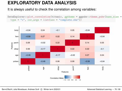
EXPLORATORY DATA ANALYSISIt is always useful to check the correlation among variables:
DataExplorer::plot_correlation(titanic, ggtheme = ggpubr::theme_pubr(base_size = 10),type = "c", cor_args = list(use = "complete.obs"))
1 −0.49 0.06 0.09 −0.59 −0.04
−0.49 1 −0.17 −0.02 0.27 0.04
0.06 −0.17 1 0.22 0.22 −0.1
0.09 −0.02 0.22 1 0.14 0.05
−0.59 0.27 0.22 0.14 1 −0.04
−0.04 0.04 −0.1 0.05 −0.04 1
pclass
age
sibsp
parch
fare
bodypc
lass
age
sibs
p
parc
h
fare
body
Features
Feat
ures
−1.0 −0.5 0.0 0.5 1.0Correlation Meter
Bernd Bischl, Julia Moosbauer, Andreas Groll c� Winter term 2020/21 Advanced Statistical Learning – 76 / 99

Breast Cancer Data Set
Bernd Bischl, Julia Moosbauer, Andreas Groll c� Winter term 2020/21 Advanced Statistical Learning – 77 / 99

BREAST CANCER DATA SET
Dataset with information on the diagnosis of breast tissues (Class; M= malignant, B = benign). Features are computed from a digitizedimage of a fine needle aspirate (FNA) of a breast mass. They describecharacteristics of the cell nuclei present in the image.
Source: https://www.kaggle.com/uciml/breast-cancer-wisconsin-data
Bernd Bischl, Julia Moosbauer, Andreas Groll c� Winter term 2020/21 Advanced Statistical Learning – 78 / 99

IMPORTING THE DATA
We use OpenML (R-Package) to download the dataset in amachine-readable format and convert it into a data.frame:
# load the dataset from OpenML Library
d = OpenML::getOMLDataSet(data.id = 15)
# convert the OpenML object to a tibble (enhanced data.frame)
bc = tibble::as_tibble(d)
Bernd Bischl, Julia Moosbauer, Andreas Groll c� Winter term 2020/21 Advanced Statistical Learning – 79 / 99

EXPLORATORY DATA ANALYSIS
print(bc)
## # A tibble: 699 x 10## Clump_Thickness Cell_Size_Unifo~ Cell_Shape_Unif~ Marginal_Adhesi~ Single_Epi_Cell~## <dbl> <dbl> <dbl> <dbl> <dbl>## 1 5 1 1 1 2## 2 5 4 4 5 7## 3 3 1 1 1 2## 4 6 8 8 1 3## 5 4 1 1 3 2## 6 8 10 10 8 7## 7 1 1 1 1 2## 8 2 1 2 1 2## 9 2 1 1 1 2## 10 4 2 1 1 2## # ... with 689 more rows, and 5 more variables: Bare_Nuclei <dbl>, Bland_Chromatin <dbl>,## # Normal_Nucleoli <dbl>, Mitoses <dbl>, Class <fct>
Bernd Bischl, Julia Moosbauer, Andreas Groll c� Winter term 2020/21 Advanced Statistical Learning – 80 / 99

EXPLORATORY DATA ANALYSISFactor variables
skimr::partition(skim(bc)) %>%.$factor %>%knitr::kable(format = ’latex’, booktabs = TRUE) %>%kableExtra::kable_styling(latex_options = ’HOLD_position’, font_size = 7)
skim_variable n_missing complete_rate ordered n_unique top_counts
Class 0 1 FALSE 2 ben: 458, mal: 241
Bernd Bischl, Julia Moosbauer, Andreas Groll c� Winter term 2020/21 Advanced Statistical Learning – 81 / 99
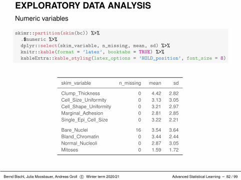
EXPLORATORY DATA ANALYSISNumeric variables
skimr::partition(skim(bc)) %>%.$numeric %>%dplyr::select(skim_variable, n_missing, mean, sd) %>%knitr::kable(format = ’latex’, booktabs = TRUE) %>%kableExtra::kable_styling(latex_options = ’HOLD_position’, font_size = 8)
skim_variable n_missing mean sd
Clump_Thickness 0 4.42 2.82Cell_Size_Uniformity 0 3.13 3.05Cell_Shape_Uniformity 0 3.21 2.97Marginal_Adhesion 0 2.81 2.85Single_Epi_Cell_Size 0 3.22 2.21
Bare_Nuclei 16 3.54 3.64Bland_Chromatin 0 3.44 2.44Normal_Nucleoli 0 2.87 3.05Mitoses 0 1.59 1.72
Bernd Bischl, Julia Moosbauer, Andreas Groll c� Winter term 2020/21 Advanced Statistical Learning – 82 / 99

EXPLORATORY DATA ANALYSISBarplots of discrete features
DataExplorer::plot_bar(bc, ggtheme = ggpubr::theme_pubr())
Class
0 100 200 300 400
malignant
benign
Frequency
Bernd Bischl, Julia Moosbauer, Andreas Groll c� Winter term 2020/21 Advanced Statistical Learning – 83 / 99

EXPLORATORY DATA ANALYSISHistograms of numerical features
DataExplorer::plot_histogram(bc, ggtheme = ggpubr::theme_pubr())
Single_Epi_Cell_Size
Clump_Thickness Marginal_Adhesion Mitoses Normal_Nucleoli
Bare_Nuclei Bland_Chromatin Cell_Shape_Uniformity Cell_Size_Uniformity
2.5 5.0 7.5 10.0
2.5 5.0 7.5 10.0 2.5 5.0 7.5 10.0 2.5 5.0 7.5 10.0 2.5 5.0 7.5 10.0
2.5 5.0 7.5 10.0 2.5 5.0 7.5 10.0 2.5 5.0 7.5 10.0 2.5 5.0 7.5 10.00
100200300400
0100200300400
0100200300
0200400600
050100150
0100200300400
0100200300400
050100150
0100200300400
value
Frequency
Bernd Bischl, Julia Moosbauer, Andreas Groll c� Winter term 2020/21 Advanced Statistical Learning – 84 / 99

EXPLORATORY DATA ANALYSISLet’s take a look at the correlation among the variables:
DataExplorer::plot_correlation(bc, ggtheme = ggpubr::theme_pubr(base_size = 8))
1 0.64 0.65 0.49 0.52 0.56 0.54 0.35 −0.72 0.720.64 1 0.91 0.71 0.75 0.76 0.72 0.46 −0.82 0.820.65 0.91 1 0.68 0.72 0.74 0.72 0.44 −0.82 0.820.49 0.71 0.68 1 0.6 0.67 0.6 0.42 −0.7 0.70.52 0.75 0.72 0.6 1 0.62 0.63 0.48 −0.68 0.68
10.56 0.76 0.74 0.67 0.62 1 0.67 0.34 −0.76 0.760.54 0.72 0.72 0.6 0.63 0.67 1 0.43 −0.71 0.710.35 0.46 0.44 0.42 0.48 0.34 0.43 1 −0.42 0.42−0.72 −0.82 −0.82 −0.7 −0.68 −0.76 −0.71 −0.42 1 −10.72 0.82 0.82 0.7 0.68 0.76 0.71 0.42 −1 1
Clump_Thickness
Cell_Size_Uniformity
Cell_Shape_Uniformity
Marginal_Adhesion
Single_Epi_Cell_Size
Bare_Nuclei
Bland_Chromatin
Normal_Nucleoli
Mitoses
Class_benign
Class_malignant
Clu
mp_
Thic
knes
s
Cel
l_Si
ze_U
nifo
rmity
Cel
l_Sh
ape_
Uni
form
ity
Mar
gina
l_Ad
hesi
on
Sing
le_E
pi_C
ell_
Size
Bare
_Nuc
lei
Blan
d_C
hrom
atin
Nor
mal
_Nuc
leol
i
Mito
ses
Cla
ss_b
enig
n
Cla
ss_m
alig
nant
Features
Feat
ures
−1.0 −0.5 0.0 0.5 1.0Correlation Meter
Bernd Bischl, Julia Moosbauer, Andreas Groll c� Winter term 2020/21 Advanced Statistical Learning – 85 / 99

EXPLORATORY DATA ANALYSISIt seems that we have quite some missing observations. Let’s take acloser look:
DataExplorer::plot_missing(bc, ggtheme = ggpubr::theme_pubr())
0%
0%
0%
0%
0%
2.29%
0%
0%
0%
0%
Bare_Nuclei
Clump_Thickness
Cell_Size_Uniformity
Cell_Shape_Uniformity
Marginal_Adhesion
Single_Epi_Cell_Size
Bland_Chromatin
Normal_Nucleoli
Mitoses
Class
0 5 10 15Missing Rows
Feat
ures
Band Good
Bernd Bischl, Julia Moosbauer, Andreas Groll c� Winter term 2020/21 Advanced Statistical Learning – 86 / 99

Forbes Data
Bernd Bischl, Julia Moosbauer, Andreas Groll c� Winter term 2020/21 Advanced Statistical Learning – 87 / 99

FORBES DATA
The Forbes2000 data include the top 2000 list of world leadingcompanies from the year 2004. The data are collected from the wellknown *Forbes Magazine*.
The magazine is well known for its lists andrankings, including of the richest Americans(the Forbes 400), of the world’s top com-panies (the Forbes Global 2000), and TheWorld’s Billionaires.
Source: https://en.wikipedia.org/wiki/Forbes
Bernd Bischl, Julia Moosbauer, Andreas Groll c� Winter term 2020/21 Advanced Statistical Learning – 88 / 99

FORBES DATAThe HSAUR2 package provides the data set, which can be imported intoR via
## rank name country category sales profits assets marketvalue## 1 1 Citigroup United States Banking 94.7 17.85 1264 255## 2 2 General Electric United States Conglomerates 134.2 15.59 627 329## 3 3 American Intl Group United States Insurance 76.7 6.46 648 195## 4 4 ExxonMobil United States Oil & gas operations 222.9 20.96 167 277## 5 5 BP United Kingdom Oil & gas operations 232.6 10.27 178 174## 6 6 Bank of America United States Banking 49.0 10.81 736 118
Note: Not all data sets contained in R packages do have help files.
Bernd Bischl, Julia Moosbauer, Andreas Groll c� Winter term 2020/21 Advanced Statistical Learning – 89 / 99

FORBES DATAFor each company, the following eight variables are available:
rank : the ranking of the company,
name : the name of the company,
country : where the company is situated,
category : products the company produces,
sales : the amount of sales of the company, US dollars,
profits : the profit of the company,
assets : the assets of the company,
marketvalue : the market value of the company.
Bernd Bischl, Julia Moosbauer, Andreas Groll c� Winter term 2020/21 Advanced Statistical Learning – 90 / 99

Heptathlon Data
Bernd Bischl, Julia Moosbauer, Andreas Groll c� Winter term 2020/21 Advanced Statistical Learning – 91 / 99

HEPTATHLON DATAThe heptathlon data includes 25 athletes of the Olympic Heptathlonin Seoul 1988. The dataset can be loaded after insatlling the HSAUR3package via:
data("heptathlon", package = "HSAUR3")
Source:https://en.wikipedia.org/wiki/1988_Summer_Olympics
Bernd Bischl, Julia Moosbauer, Andreas Groll c� Winter term 2020/21 Advanced Statistical Learning – 92 / 99

HEPTATHLON DATAThe heptathlon datasets includes the the results of each of the sevendisciplins:
## hurdles highjump shot run200m longjump javelin run800m score## Joyner-Kersee (USA) 12.7 1.86 15.8 22.6 7.27 45.7 129 7291## John (GDR) 12.8 1.80 16.2 23.6 6.71 42.6 126 6897## Behmer (GDR) 13.2 1.83 14.2 23.1 6.68 44.5 124 6858## Sablovskaite (URS) 13.6 1.80 15.2 23.9 6.25 42.8 132 6540## Choubenkova (URS) 13.5 1.74 14.8 23.9 6.32 47.5 128 6540## Schulz (GDR) 13.8 1.83 13.5 24.6 6.33 42.8 126 6411
Bernd Bischl, Julia Moosbauer, Andreas Groll c� Winter term 2020/21 Advanced Statistical Learning – 93 / 99

Flights Data
Bernd Bischl, Julia Moosbauer, Andreas Groll c� Winter term 2020/21 Advanced Statistical Learning – 94 / 99
FLIGHTS DATA
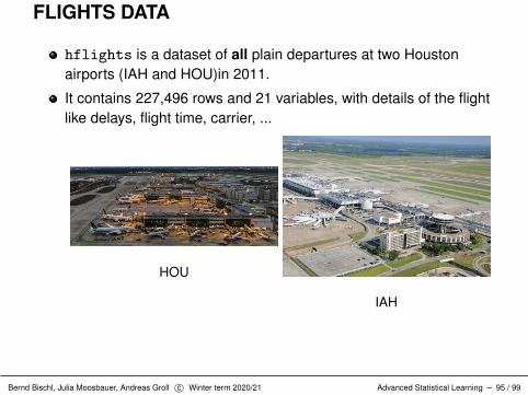
hflights is a dataset of all plain departures at two Houstonairports (IAH and HOU)in 2011.
It contains 227,496 rows and 21 variables, with details of the flightlike delays, flight time, carrier, ...
HOU
IAH
Bernd Bischl, Julia Moosbauer, Andreas Groll c� Winter term 2020/21 Advanced Statistical Learning – 95 / 99

FLIGHTS DATAThe dataset is contained within an additional package also calledhflights
The package needs to be installed and loaded to access the data:
## Year Month DayofMonth## Min. :2011 Min. : 1.00 Min. : 1.0## 1st Qu.:2011 1st Qu.: 4.00 1st Qu.: 8.0## Median :2011 Median : 7.00 Median :16.0## Mean :2011 Mean : 6.51 Mean :15.7## 3rd Qu.:2011 3rd Qu.: 9.00 3rd Qu.:23.0## Max. :2011 Max. :12.00 Max. :31.0
Bernd Bischl, Julia Moosbauer, Andreas Groll c� Winter term 2020/21 Advanced Statistical Learning – 96 / 99

Munich Rent Index
Bernd Bischl, Julia Moosbauer, Andreas Groll c� Winter term 2020/21 Advanced Statistical Learning – 97 / 99

MUNICH RENT INDEX 2015
The Munich rent index is published by Prof. Kauermann and MichaelWindmann from the Department of Statistics at the LMU. The data weprovide is anonymised and reduced to 1000 observations:
kable(rbind(head(rent15), c("...")))
rent size rooms year good best hw0 ch0 bathtiled0 bathextra kitchen822.6 110 5 1957.5 0 0 0 1 1 1 0595 70 3 1972 0 0 0 0 0 0 01100 91 4 2000.5 0 0 0 0 1 1 0693.36 64 3 1957.5 0 0 0 0 1 0 0700 56 2 1992.5 0 0 0 0 1 1 1686 55 2 2000.5 0 0 0 0 1 0 1... ... ... ... ... ... ... ... ... ... ...
Bernd Bischl, Julia Moosbauer, Andreas Groll c� Winter term 2020/21 Advanced Statistical Learning – 98 / 99

MUNICH RENT INDEX 2015The data contains the following variables:
rent: the net rent in euros.
size: living space in square meter.
rooms: number of rooms.
year: year of construction.
good: good address / residential area (yes: 1, no: 0).
best: best address / residential area (yes: 1, no: 0).
hw0: hot water supply (1: no, 0: yes).
ch0: central heating (1: no, 0: yes).
bathtiled0: tiled bathroom (1: no, 0: yes).
bathextra: special furniture in bathroom (1: yes, 0: no).
kitchen: well equipped kitchen (1: yes, 0: no).
Bernd Bischl, Julia Moosbauer, Andreas Groll c� Winter term 2020/21 Advanced Statistical Learning – 99 / 99

Advanced Statistical Learning
Chapter 0: Notation and definitions
Bernd Bischl, Julia Moosbauer, Andreas Groll
Department of Statistics – TU Dortmund
Winter term 2020/21

FUNDAMENTAL DEFINITIONS AND NOTATION
X : p-dim. input space, usually we assume X = Rp, butcategorical features can occur as well.
Y : target space, e.g. Y = R, Y = {0, 1}, Y = {�1, 1},Y = {1, . . . , g} or Y = {label1 . . . label
g
}x : feature vector, x = (x1, . . . , xp
)T 2 Xy : target / label / output. y 2 YP
xy
: joint probability distribution on X ⇥ Yp(x, y) or p(x, y | ✓) : joint pdf for x and y
Bernd Bischl, Julia Moosbauer, Andreas Groll c� Winter term 2020/21 Advanced Statistical Learning – 1 / 7

FUNDAMENTAL DEFINITIONS AND NOTATIONRemark:This lecture is mainly developed from a frequentist perspective. Ifparameters appear behind the "|", this is for better reading, and doesnot imply that we condition on them in a Bayesian sense (but thisnotation would actually make a Bayesian treatment simple). Soformally, p(x|✓) should be read as p✓(x) or p(x,✓) or p(x;✓).
Bernd Bischl, Julia Moosbauer, Andreas Groll c� Winter term 2020/21 Advanced Statistical Learning – 2 / 7

FUNDAMENTAL DEFINITIONS AND NOTATION�x(i), y (i)
�: i-th observation or instance
D =��
x(1), y (1)�, . . . ,
�x(n), y (n)
� : data set with n observations
Dtrain, Dtest : data for training and testing, often D = Dtrain[ Dtest
f (x) or f (x | ✓) 2 R or Rg : prediction function (model) learnedfrom data, we might suppress ✓ in notation
h(x) or h(x|✓) 2 Y : discrete prediction for classification (see later)
✓ 2 ⇥ : model parameters(some models may traditionally use different symbols)
H : hypothesis space. f lives here; it restricts the functional formof f
✏ = y � f (x) or ✏(i) = y
(i) � f
�x(i)
�: residual in regression
yf (x) or y
(i)f
�x(i)
�: margin for binary classification with
Y = {�1, 1} (see later)
Bernd Bischl, Julia Moosbauer, Andreas Groll c� Winter term 2020/21 Advanced Statistical Learning – 3 / 7

FUNDAMENTAL DEFINITIONS AND NOTATION⇡
k
(x) = P(y = k | x) : posterior probability for class k , given x, incase of binary labels we might abbreviate ⇡(x) = P(y = 1 | x)
⇡k
= P(y = k) : prior probability for class k , in case of binarylabels we might abbreviate ⇡ = P(y = 1)
L(✓) and `(✓) : Likelihood and log-Likelihood for a parameter ✓,based on a statistical model
f , h, ⇡k
(x), ⇡(x) and ✓ : learned functions and parameters
Remark: With a slight abuse of notation we write random variables,e.g., x and y , in lowercase, as normal variables or function arguments.The context will make clear what is meant.
Bernd Bischl, Julia Moosbauer, Andreas Groll c� Winter term 2020/21 Advanced Statistical Learning – 4 / 7

FUNDAMENTAL DEFINITIONS AND NOTATIONIn the simplest case we have i.i.d. data D, where the input and outputspace are both real-valued and one-dimensional.
10
15
20
25
30
35
2 3 4 5x
y
Bernd Bischl, Julia Moosbauer, Andreas Groll c� Winter term 2020/21 Advanced Statistical Learning – 5 / 7

FUNDAMENTAL DEFINITIONS AND NOTATIONDesign matrix (with or w/o intercept term):
X =
0
B@x
(1)1 · · · x
(1)p
......
...
x
(n)1 · · · x
(n)p
1
CA X =
0
B@1 x
(1)1 · · · x
(1)p
......
......
1 x
(n)1 · · · x
(n)p
1
CA
xj
=⇣
x
(1)j
, . . . , x(n)j
⌘T
: j-th observed feature vector.
y =�y
(1), . . . , y (n)�
T
: vector of target values.
The design matrix on the right demonstrates the trick to encodethe intercept via an additional constant-1 feature, so the featurespace will be (p + 1)-dimensional. This allows to simplify notation,e.g., to write f (x) = ✓T x, instead of f (x) = ✓0 + ✓T x.
Bernd Bischl, Julia Moosbauer, Andreas Groll c� Winter term 2020/21 Advanced Statistical Learning – 6 / 7

BINARY LABEL CODING
Remark: Notation in binary classification can be sometimes confusingbecause of different coding styles, and as we have to talk aboutpredicted scores, classes and probabilities.
A binary variable can take only two possible values. For probability /likelihood-based model derivations a 0-1-coding, for geometric /loss-based models the -1/+1-coding is often preferred:
Y = {0, 1}. Here, the approach often models ⇡(x), the posteriorprobability for class 1 given x. Usually, we then defineh(x) = [⇡(x) � 0.5] 2 Y .
Y = {�1, 1}. Here, the approach often models f (x), a real-valuedscore from R given x. Usually, we define h(x) = sign(f (x)) 2 Y ,and we interpret |f (x)| as “confidence” for the predicted class h(x).
Bernd Bischl, Julia Moosbauer, Andreas Groll c� Winter term 2020/21 Advanced Statistical Learning – 7 / 7