advanced statistical methods002
TRANSCRIPT


13-1 Designing Engineering Experiments
Every experiment involves a sequence of activities:
1. Conjecture – the original hypothesis that motivates the experiment.
2. Experiment – the test performed to investigate the conjecture.
3. Analysis – the statistical analysis of the data from the experiment.
4. Conclusion – what has been learned about the original conjecture from the experiment. Often the experiment will lead to a revised conjecture, and a new experiment, and so forth.

13-2 The Completely Randomized Single-Factor Experiment
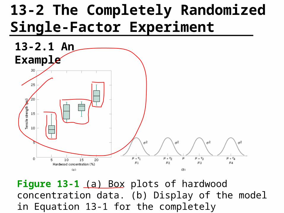
13-2.1 An Example

13-2 The Completely Randomized Single-Factor Experiment
13-2.1 An Example

13-2 The Completely Randomized Single-Factor Experiment
13-2.1 An Example
• The levels of the factor are sometimes called treatments.
• Each treatment has six observations or replicates.
• The runs are run in random order.
13-2 The Completely Randomized Single-Factor Experiment
Figure 13-1 (a) Box plots of hardwood concentration data. (b) Display of the model in Equation 13-1 for the completely randomized single-factor experiment
13-2.1 An Example
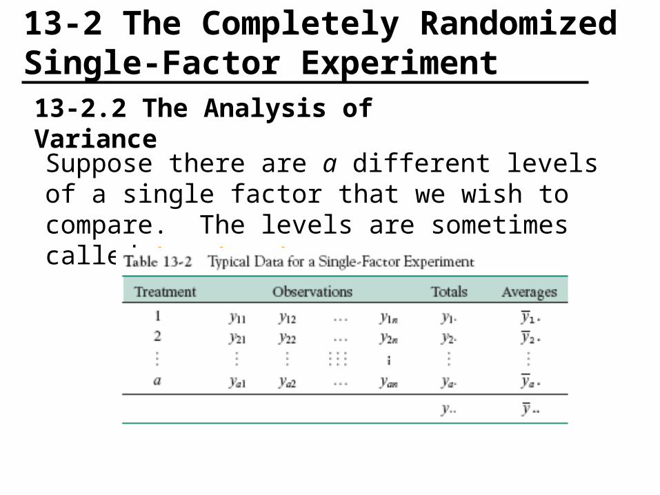
13-2 The Completely Randomized Single-Factor Experiment13-2.2 The Analysis of Variance
Suppose there are a different levels of a single factor that we wish to compare. The levels are sometimes called treatments.

13-2 The Completely Randomized Single-Factor Experiment13-2.2 The Analysis of Variance
We may describe the observations in Table 13-2 by the linear statistical model:
The model could be written as

13-2 The Completely Randomized Single-Factor Experiment13-2.2 The Analysis of Variance
Fixed-effects Model
The treatment effects are usually defined as deviations from the overall mean so that:
Also,

13-2 The Completely Randomized Single-Factor Experiment13-2.2 The Analysis of Variance
We wish to test the hypotheses:
The analysis of variance partitions the total variability into two parts.

13-2 The Completely Randomized Single-Factor Experiment13-2.2 The Analysis of Variance
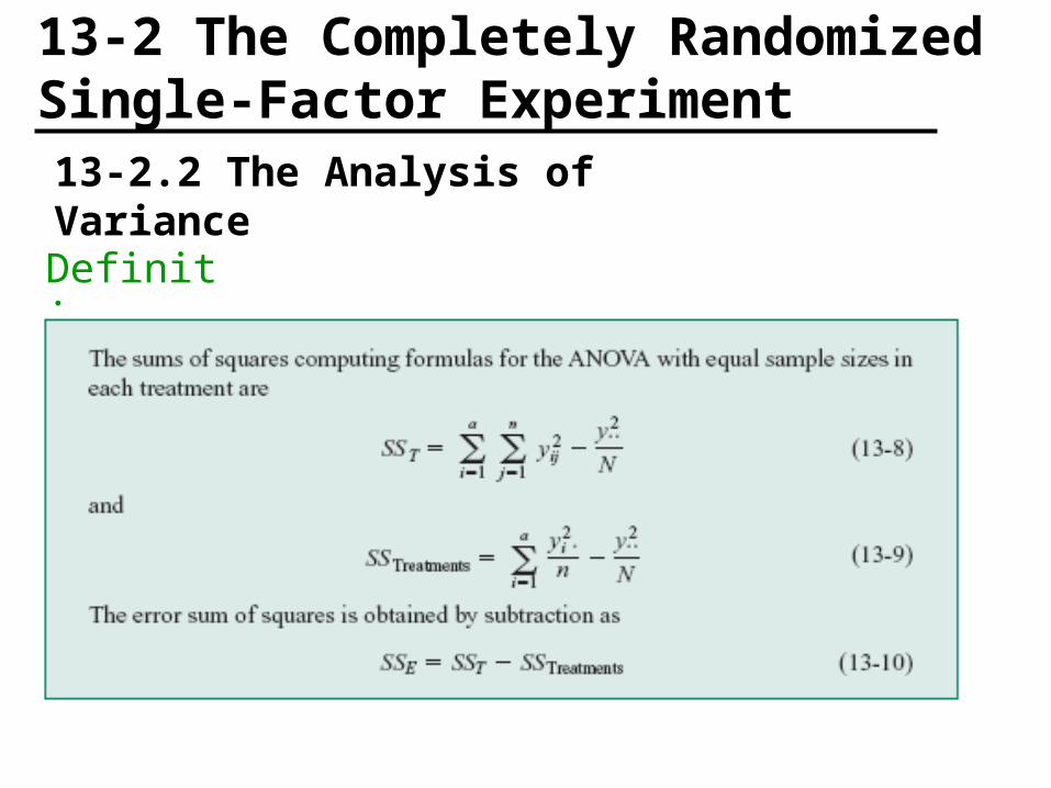
Definition
13-2 The Completely Randomized Single-Factor Experiment13-2.2 The Analysis of Variance
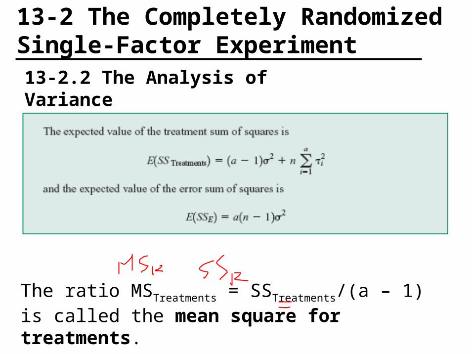
The ratio MSTreatments = SSTreatments/(a – 1) is called the mean square for treatments.

13-2 The Completely Randomized Single-Factor Experiment13-2.2 The Analysis of Variance
The appropriate test statistic is
We would reject H0 if f0 > f,a-1,a(n-1)
13-2 The Completely Randomized Single-Factor Experiment13-2.2 The Analysis of Variance
Definition

13-2 The Completely Randomized Single-Factor Experiment13-2.2 The Analysis of Variance
Analysis of Variance Table

13-2 The Completely Randomized Single-Factor Experiment
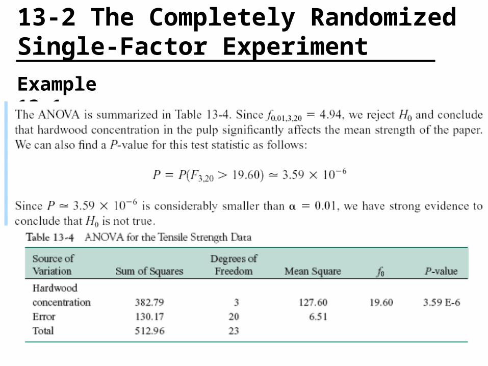
Example 13-1

13-2 The Completely Randomized Single-Factor Experiment
Example 13-1
13-2 The Completely Randomized Single-Factor Experiment
Example 13-1


13-2 The Completely Randomized Single-Factor Experiment
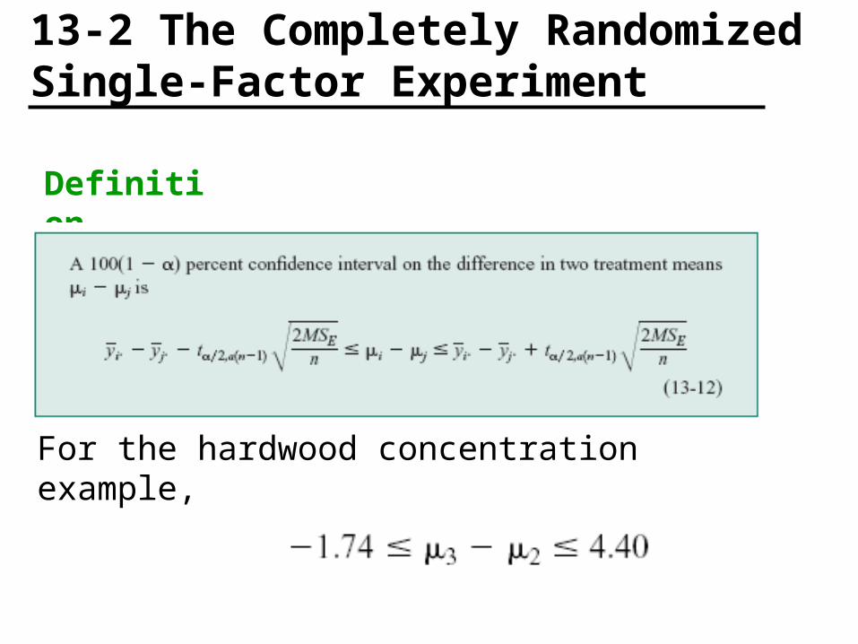
Definition
For 20% hardwood, the resulting confidence interval on the mean is
13-2 The Completely Randomized Single-Factor Experiment
Definition
For the hardwood concentration example,

13-2 The Completely Randomized Single-Factor Experiment
An Unbalanced Experiment
13-2 The Completely Randomized Single-Factor Experiment
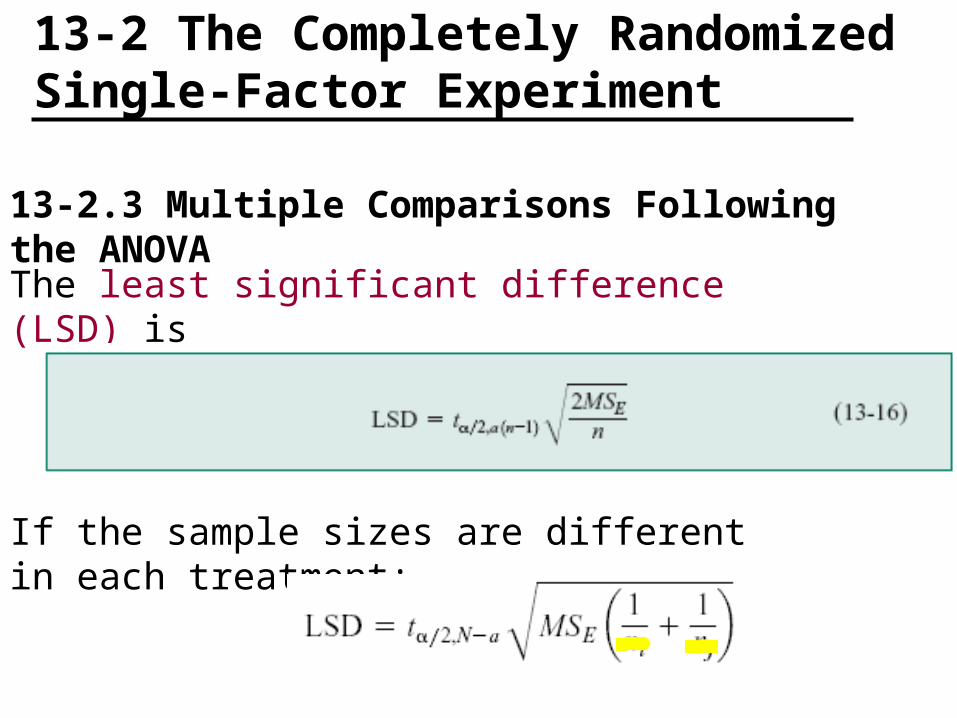
13-2.3 Multiple Comparisons Following the ANOVA
The least significant difference (LSD) is
If the sample sizes are different in each treatment:

13-2 The Completely Randomized Single-Factor Experiment
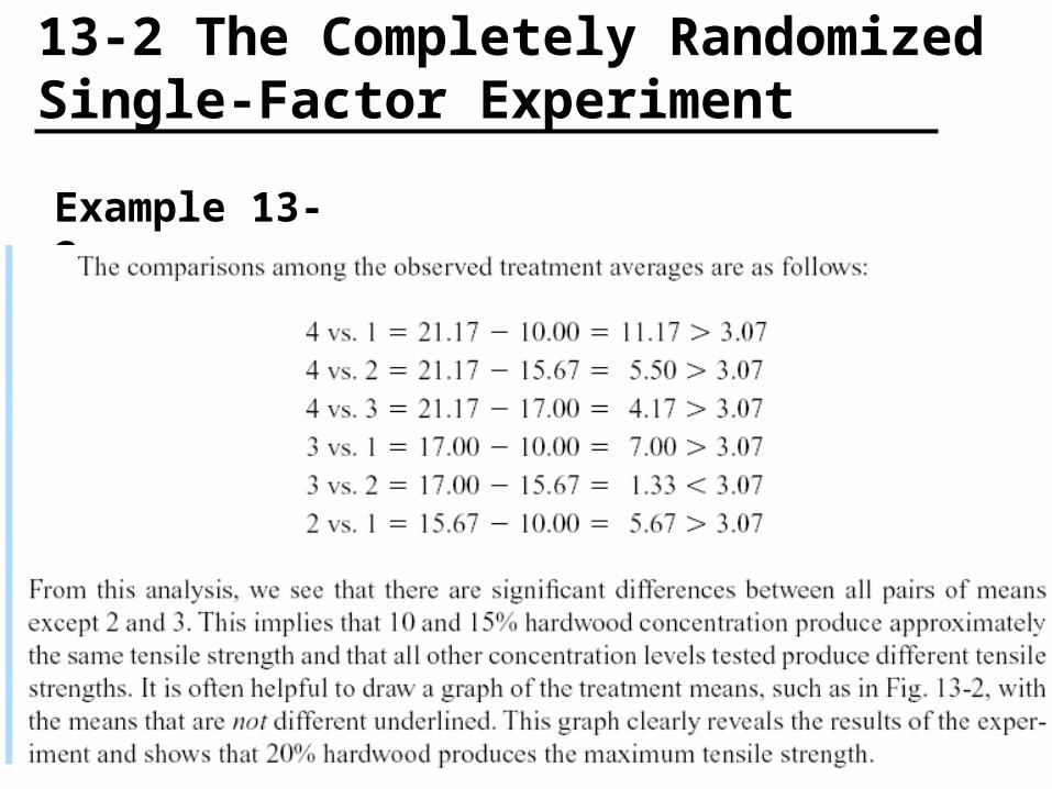
Example 13-2
13-2 The Completely Randomized Single-Factor Experiment
Example 13-2

13-2 The Completely Randomized Single-Factor Experiment
Example 13-2
Figure 13-2 Results of Fisher’s LSD method in Example 13-2

13-2 The Completely Randomized Single-Factor Experiment
13-2.5 Residual Analysis and Model Checking

13-2 The Completely Randomized Single-Factor Experiment
13-2.5 Residual Analysis and Model Checking
Figure 13-4 Normal probability plot of residuals from the hardwood concentration experiment.

13-2 The Completely Randomized Single-Factor Experiment
13-2.5 Residual Analysis and Model Checking
Figure 13-5 Plot of residuals versus factor levels (hardwood concentration).

13-2 The Completely Randomized Single-Factor Experiment
13-2.5 Residual Analysis and Model Checking
Figure 13-6 Plot of residuals versus iy

13-3 The Random-Effects Model
13-3.1 Fixed versus Random Factors

13-3 The Random-Effects Model
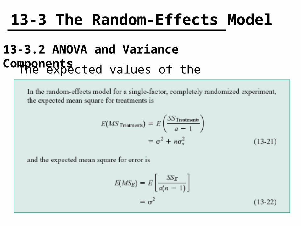
13-3.2 ANOVA and Variance Components
The linear statistical model is
The variance of the response is
Where each term on the right hand side is called a variance component.

13-3 The Random-Effects Model
13-3.2 ANOVA and Variance Components
For a random-effects model, the appropriate hypotheses to test are:
The ANOVA decomposition of total variability is still valid:
13-3 The Random-Effects Model
13-3.2 ANOVA and Variance Components
The expected values of the mean squares are

13-3 The Random-Effects Model
13-3.2 ANOVA and Variance Components
The estimators of the variance components are

13-3 The Random-Effects Model
Example 13-4

13-3 The Random-Effects Model
Example 13-4

13-3 The Random-Effects Model
Figure 13-8 The distribution of fabric strength. (a) Current process, (b) improved process.

13-4 Randomized Complete Block Designs
13-4.1 Design and Statistical Analyses
The randomized block design is an extension of the paired t-test to situations where the factor of interest has more than two levels.
Figure 13-9 A randomized complete block design.

13-4 Randomized Complete Block Designs
13-4.1 Design and Statistical Analyses
For example, consider the situation of Example 10-9, where two different methods were used to predict the shear strength of steel plate girders. Say we use four girders as the experimental units.

13-4 Randomized Complete Block Designs
13-4.1 Design and Statistical Analyses
General procedure for a randomized complete block design:

13-4 Randomized Complete Block Designs
13-4.1 Design and Statistical Analyses
The appropriate linear statistical model:
We assume
• treatments and blocks are initially fixed effects
• blocks do not interact
•

13-4 Randomized Complete Block Designs
13-4.1 Design and Statistical Analyses
We are interested in testing:

13-4 Randomized Complete Block Designs
13-4.1 Design and Statistical Analyses
The mean squares are:
13-4 Randomized Complete Block Designs
13-4.1 Design and Statistical Analyses
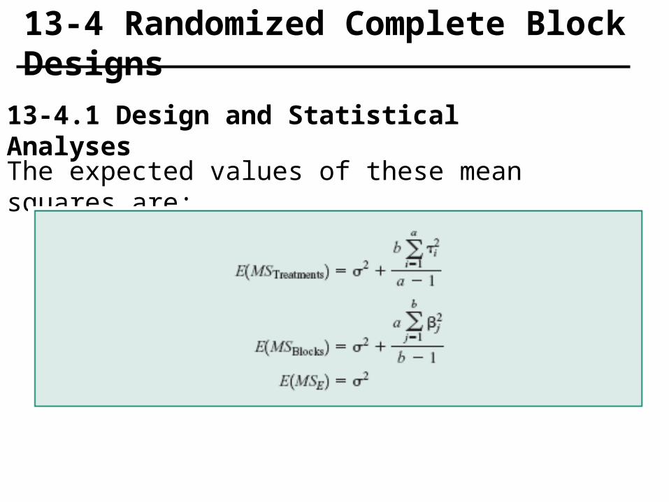
The expected values of these mean squares are:

13-4 Randomized Complete Block Designs
13-4.1 Design and Statistical Analyses
Definition

13-4 Randomized Complete Block Designs
13-4.1 Design and Statistical Analyses

13-4 Randomized Complete Block Designs
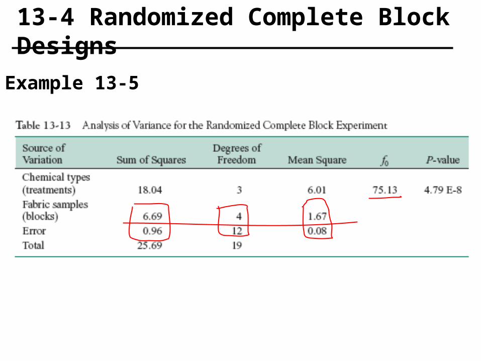
Example 13-5

13-4 Randomized Complete Block Designs
Example 13-5

13-4 Randomized Complete Block Designs
Example 13-5
13-4 Randomized Complete Block Designs
Example 13-5

13-4 Randomized Complete Block Designs
Minitab Output for Example 13-5

13-4 Randomized Complete Block Designs
13-4.2 Multiple Comparisons
Fisher’s Least Significant Difference for Example 13-5
Figure 13-10 Results of Fisher’s LSD method.

13-4 Randomized Complete Block Designs
13-4.3 Residual Analysis and Model Checking
Figure 13-11 Normal probability plot of residuals from the randomized complete block design.

13-4 Randomized Complete Block Designs
Figure 13-12 Residuals by treatment.

13-4 Randomized Complete Block Designs
Figure 13-13 Residuals by block.
13-4 Randomized Complete Block Designs
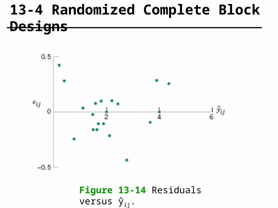
Figure 13-14 Residuals versus ŷij.
