advances in abstract categorial grammars
TRANSCRIPT

Advances in Abstract Categorial Grammars
Language Theory and Linguistic Modeling
Lecture 3
Reduction of second-order ACGs to to DatalogExtension to “almost linear” second-order ACGs
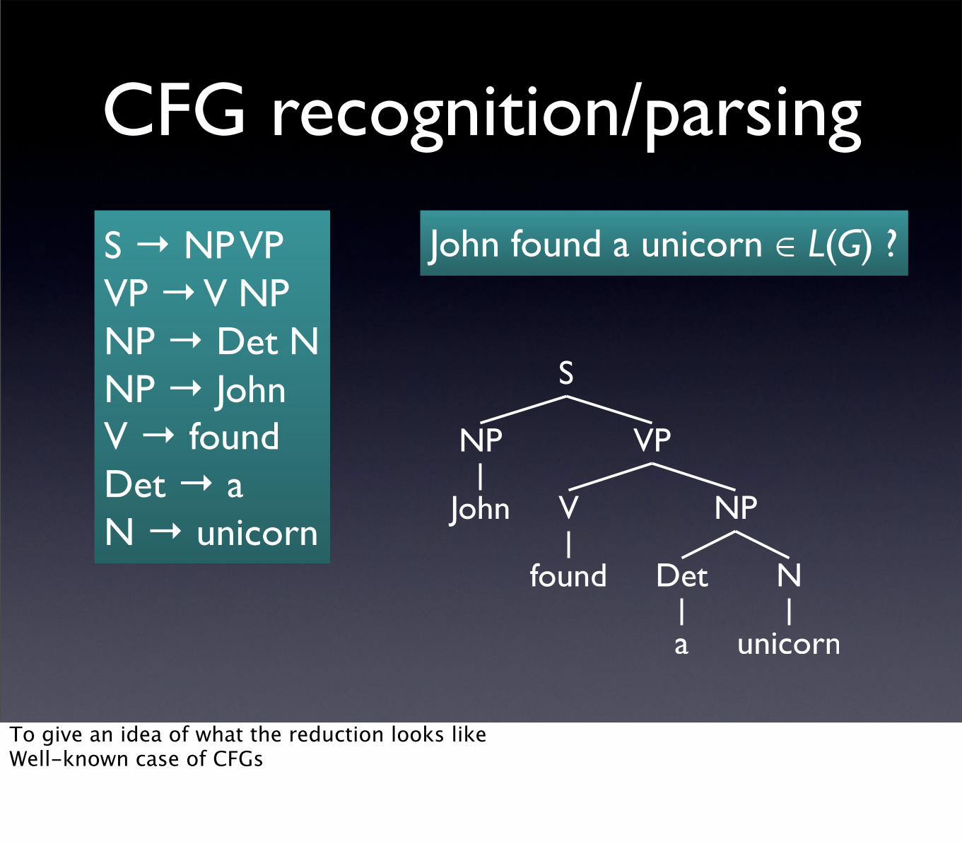
CFG recognition/parsing
S → NP VPVP → V NPNP → Det NNP → JohnV → foundDet → aN → unicorn
John found a unicorn ∈ L(G) ?
To give an idea of what the reduction looks likeWell-known case of CFGs

Datalog query evaluation
S(i, k) :- NP(i, j), VP(j, k).VP(i, k) :- V(i, j), NP(j, k).NP(i, k) :- Det(i, j), N(j, k).NP(i, j) :- John(i, j).V(i, j) :- found(i, j).Det(i, j) :- a(i, j).N(i, j) :- unicorn(i, j).
John(0, 1).found(1, 2).a(2, 3).unicorn(3, 4).
?- S(0, 4).program
database
query
Definite clause grammar representationExecutable as Prolog code

0 1John found 2 a 3 unicorn 4
John(0, 1) found(1, 2) a(2, 3) unicorn(3, 4)
i jNP VP k
S(i, k) :- NP(i, j), VP(j, k).
?- S(0, 4).
The conversion is very straightforwardString -> string graph

CFG recognition/parsing ≈ Datalog query evaluation
CFG derivation tree and Datalog derivation tree isomorphic to each otherFinding one amounts to finding the other

Recognition/Parsing
almost linearsecond-order
ACGs
Parsing and generation as Datalog query evaluation
Recognition/Parsing
Generation
CFGMCFGRTG
MRTGCFTGIO
…
CFG, etc. + Montague semantics†
† when almost linear
Kanazawa 2007
Datalog queryevaluation
The Datalog representation extends to various grammars through (almost linear) second-order ACGsNeed non-linear terms to represent logical formulas

Parsing and generation as Datalog query evaluation
• Algorithms
- Seminaive bottom-up ≈ CYK
- Magic-sets rewriting ≈ Earley
• Computational complexity
- Fixed grammar recognition
- Uniform recognition
- Parsing
Allows a uniform approach to parsing and generationSophisticated evaluation methods for Datalog apply to parsing/generation

Polynomial-time algorithm
facts that immediately follow from one fact in agenda[i] plus
some facts in chart
holds facts with derivation tree of minimal height i
≈ well-formed substring table
Works for Datalog programs in general

Outputting shared forest
instances of rules with right-hand side consisting of
one fact in agenda[i] and some facts in chart
holds instances of rules that can be used in derivation
trees
shared parse forest
facts that immediately follow from one fact in agenda[i] plus
some facts in chart
Parsing algorithms are often not explicitly stated in textbooks.

Computational complexity
• CFG
Fixed grammar recognition
Uniform recognition
ε-free uniform recognition
LOGCFL-complete
P-complete
LOGCFL-complete
Same holds for classes of grammars that can be represented by Datalog programs of bounded degree

Computational complexity
• Almost linear second-order ACGs with bounded width and rank
Fixed grammar recognition
Uniform recognition
ε-free uniform recognition
LOGCFL-complete
P-complete
LOGCFL-complete
width = |σ(B)| = arity of B in Datalogrank = number of subgoals
ε-rule = Datalog rule with empty right-hand sideε-rule = rule whose right-hand side is empty and whose left-hand side argument is a pure λ-term

LOGCFL
• The class of problems that reduce to some context-free language in logarithmic space
• The smallest computational complexity class that includes the context-free languages
AC0 ⊆ NC1 ⊆ L ⊆ NL ⊆ LOGCFL ⊆ AC1 ⊆ NC2 ⊆ P ⊆ NP
A very important complexity classImplies the existence of efficient parallel algorithm

Datalog in computational linguistics
• Definite Clause Grammar
• Deduction system
• Uninstantiated parsing system
Pereira and Warren 1980
Shieber et al. 1997
Sikkel 1997
[NP, i, j] [VP, j, k][S, i, k]
The idea of using Datalog is not new.DCG is too powerful.Datalog notation is more convenient.

CFG + Montague semantics
S(X1X
2)→ NP(X
1) VP(X
2)
VP(λx .X2(λy .X
1yx ))→ V(X
1) NP(X
2)
V(λyx .X2(X
1yx )(X
3yx ))→ V(X
1) Conj(X
2) V(X
3)
NP(X1X
2)→ Det(X
1) N(X
2)
NP(λu.u Johne )→ John
V(finde→e→t )→ found
V(catche→e→t )→ caught
Conj(∧ t→t→t )→ and
Det(λuv .∃(e→t )→t (λy .∧ t→t→t (uy )(vy )))→ a
N(unicorne→t )→ unicorn
λuv .∃y(u(y )∧ v(y ))
One way of writing Montague semantics with CFG

(λu.u John)(λx .(λuv .∃(λy .∧(uy )(vy ))unicorn(λy .find y x ))
∃(λy .∧(unicorn y )(find y John))↠β
∃y(unicorn(y )∧ find(John, y ))≈logical form
Grammar rules associates a lambda-term to each nodeMust reduce to normal form to get the desired representation
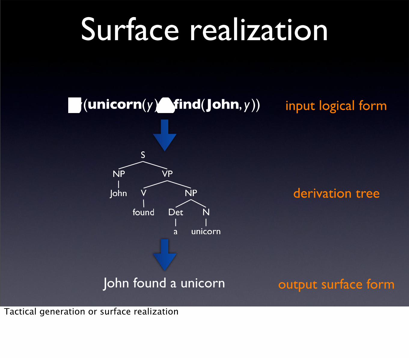
Surface realization
John found a unicorn
∃y(unicorn(y )∧ find(John, y )) input logical form
output surface form
derivation tree
Tactical generation or surface realization

Parsing of input logical form
∃y(unicorn(y )∧ find(John, y )) input logical form
derivation tree
Can concentrate on the semantic half of the grammar

Recognition of surface realizability
∃y(unicorn(y )∧ find(John, y )) input logical form
yes/no
surface realizable?
Solving this problem almost amounts to solving surface realization

Context-free grammar on λ-terms
S(X1X
2) :−NP(X
1), VP(X
2)
VP(λx .X2(λy .X
1yx )) :− V(X
1),NP(X
2).
V(λyx .X2(X
1yx )(X
3yx )) :− V(X
1),Conj(X
2), V(X
3).
NP(X1X
2) :−Det(X
1),N(X
2).
NP(λu.u Johne ).
V(finde→e→t ).
V(catche→e→t ).
Conj(∧ t→t→t ).
Det(λuv .∃(e→t )→t (λy .∧ t→t→t (uy )(vy ))).
N(unicorne→t ).
CFG + Montague - CFG = CFLGGenerates a set of lambda-terms

Context-free grammar on λ-terms
S(X1X
2) :−NP(X
1), VP(X
2)
VP(λx .X2(λy .X
1yx )) :− V(X
1),NP(X
2).
V(λyx .X2(X
1yx )(X
3yx )) :− V(X
1),Conj(X
2), V(X
3).
NP(X1X
2) :−Det(X
1),N(X
2).
NP(λu.u Johne ).
V(finde→e→t ).
V(catche→e→t ).
Conj(∧ t→t→t ).
Det(λuv .∃(e→t )→t (λy .∧ t→t→t (uy )(vy ))).
N(unicorne→t ).
σ (S) = t
σ (VP) = e → t
σ (NP) = (e → t)→ t
σ (V) = e → e → t
σ (Conj) = t → t → t
σ (Det) = (e → t)→ (e → t)→ t
σ (N) = e → t
A nonterminal is associated with a type.Arguments are λ-terms of that type.

Context-free grammars on λ-terms = second-order non-linear ACGs
π: B(M) :− B1(X
1),…,B
n(X
n).
π : B1→→ B
n→ B
abstractconstant
type of π
object realization of
π λX
1…X
n.M
L

S(X1X
2) :−NP(X
1), VP(X
2)
VP(λx .X2(λy .X
1yx )) :− V(X
1),NP(X
2).
V(λyx .X2(X
1yx )(X
3yx )) :− V(X
1),Conj(X
2), V(X
3).
NP(X1X
2) :−Det(X
1),N(X
2).
NP(λu.u Johne ).
V(finde→e→t ).
V(catche→e→t ).
Conj(∧ t→t→t ).
Det(λuv .∃(e→t )→t (λy .∧ t→t→t (uy )(vy ))).
N(unicorne→t ).
S(λz.X1(X
2z)) :−NP(X
1), VP(X
2)
VP(λz.X1(X
2z)) :− V(X
1),NP(X
2).
V(λz.X1(X
2(X
3z))) :− V(X
1),Conj(X
2), V(X
3).
NP(λz.X1(X
2z)) :−Det(X
1),N(X
2).
NP(λz. John z).
V(λz.found z).
V(λz.caught z).
Conj(λz.and z).
Det(λz.a z).
N(λz.unicorn z).
/ John found a unicorn / ∃(λy .∧(unicorn y )(find y John))
A pair of second-order (non-linear) ACGs as a “synchronous” grammar

From second-order ACG recognition to Datalog query evaluation
S(X1X
2) :−NP(X
1) VP(X
2)
VP(λx .X2(λy .X
1yx )) :− V(X
1),NP(X
2).
V(λyx .X2(X
1yx )(X
3yx )) :− V(X
1),Conj(X
2), V(X
3).
NP(X1X
2) :−Det(X
1),N(X
2).
NP(λu.u Johne ).
V(finde→e→t ).
V(catche→e→t ).
Conj(∧ t→t→t ).
Det(λuv .∃(e→t )→t (λy .∧ t→t→t (uy )(vy ))).
N(unicorne→t ).
∃(λy .∧(unicorn y )(find y John))∈L(G )?

From second-order ACG recognition to Datalog query evaluation
S(i1) :−NP(i
1, i
2, i
3) VP(i
2, i
3)
VP(i1, i
4) :− V(i
2, i
4, i
3),NP(i
1, i
2, i
3).
V(i1, i
4, i
3) :− V(i
2, i
4, i
3),Conj(i
1, i
5, i
2), V(i
5, i
4, i
3).
NP(i1, i
4, i
5) :−Det(i
1, i
4, i
5, i
2, i
3),N(i
2, i
3).
NP(i1, i
1, i
2) :− John(i
2).
V(i1, i
3, i
2) :− find(i
1, i
3, i
2).
V(i1, i
3, i
2) :− catch(i
1, i
3, i
2).
Conj(i1, i
3, i
2) :− ∧(i
1, i
3, i
2).
Det(i1, i
5, i
4, i
3, i
4) :− ∃(i
1, i
2, i
4),∧(i
2, i
5, i
3).
N(i1, i
2) :−unicorn(i
1, i
2).
∃(1,2,4).
∧(2,5,3).
unicorn(3,4).
find(5,6,4).
John(6).
?− S(1).
Given conversion to Datalog, can use general Datalog techniques.

0 1John found 2 a 3 unicorn 4
John(0, 1) found(1, 2) a(2, 3) unicorn(3, 4)
i jNP VP k
S(i, k) :- NP(i, j), VP(j, k).
?- S(0, 4).
The way the program, the database, and the query are obtained is similar to the CFG case.Objects derived by the grammar are represented by (hyper)graphs.

i1
a
∃
i2
λy
∧
i3
i4
u
y
i5
i6
v
y
∃(λy .∧(uy )(vy ))
tree graph
i1
∃
i2
∧
i3
i4
u
y
i5
v
term graph
λuv .∃(λy .∧(uy )(vy ))
term graph withexternal nodes
i1
∃
i2
∧
i3
i4
u
y
i5
v
1
2
35
4
λ-terms can also be represented by hypergraphs (when almost linear).A hypergraph is a “term graph” when each node is the “result node” of a unique hyperedge.A hyperedge is “directed”: the nodes it attaches to are ordered.

Det(λuv .∃(e→t )→t (λy .∧ t→t→t (uy )(vy ))).
i1
∃
i2
∧
i3
i4
u
y
i5
v
1
2
35
4
Det(i1, i
5, i
4, i
3, i
4) :− ∃(i
1, i
2, i
4),∧(i
2, i
5, i
3).
How a rule is converted to a Datalog rule.External nodes become arguments of the head.Edges labeled by constants become subgoals.Edges labeled by free variables (none in this example) become subgoals.

1
∃
2
∧
3
4
unicorn
y
5
find
6
John
∃(λy .∧(unicorn y )(find y John))
∃(1,2,4).
∧(2,5,3).
unicorn(3,4).
find(5,6,4).
John(6).
?− S(1).
1
How the input λ-term is converted to database and query.Edges labeled by constants constitute the database.External nodes become arguments of the query.

From ACG recognition to Datalog query evaluation• The reduction is correct when all λ-terms
in the grammar are almost linear.
λIalmost affine
Vacuous abstraction is not allowed.If a variable occurs twice in a subterm, it must have an atomic type.

Context-free grammar on λ-terms
S(X1X
2) :−NP(X
1), VP(X
2)
VP(λx .X2(λy .X
1yx )) :− V(X
1),NP(X
2).
V(λy exe .X2(X
1y exe )(X
3y exe )) :− V(X
1),Conj(X
2), V(X
3).
NP(X1X
2) :−Det(X
1),N(X
2).
NP(λu.u Johne ).
V(finde→e→t ).
V(catche→e→t ).
Conj(∧ t→t→t ).
Det(λuv .∃(e→t )→t (λy e .∧ t→t→t (uye )(vy e ))).
N(unicorne→t ).
All λ-terms almost linear.Generates β-normal forms of almost linear λ-terms.

Almost linear λ-terms
• The class of almost linear λ-terms is not closed under β-reduction.
(λxe .y e→e→t xx )(ze→ewe )→β y(zw )(zw )

A formal definition of graph(M)
λy exe .∧ t→t→t (X1e→e→t yx )(X
3yx )
A formal definition of the hypergraph associated with an almost linear λ-term.The input may have to be β-expanded first.The graph of a constant or variable of type α has |α| nodes, all of which are external.

For Mα→βNα, the last |α| external nodes of graph(M) are identified with the external nodes of graph(N).The new external nodes are the remaining external nodes of graph(M).

The edges labeled by the same variable (and the nodes they attach to) are also merged.Such a variable is atomic-typed.
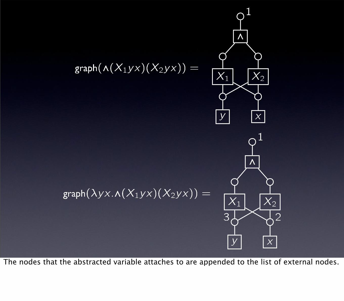
The nodes that the abstracted variable attaches to are appended to the list of external nodes.

M = λuv .∃(e→t )→t (λy .∧ t→t→t (uy )(vy ))
i1
∃
i2
∧
i3
i4
u
y
i5
v
1
2
35
4
principal typing
The construction of the graph gives a principal typing (i.e., most general typing).

Typed λ-calculus
• If M is typable, M has a unique principal typing.
• Subject Reduction:
General facts of importance.All other typings are instantiations of the principal typing.

Pure linear λ-terms
• The principal typing of an affine λ-term is balanced.
• If M has a balanced typing, it is affine.
Belnap 1976
Hirokawa 1992
Many properties of linear λ-terms carry over to almost linear.Linear = affine + λI“Balanced” means that there is at most one positive and at most one negative occurrence of any atomic type.
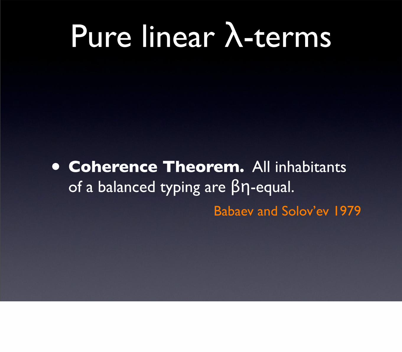
Pure linear λ-terms
• Coherence Theorem. All inhabitants of a balanced typing are βη-equal.
Babaev and Solov’ev 1979

Pure linear λ-terms
• Subject Expansion Theorem.
non-erasingnon-duplicating Hindley
β

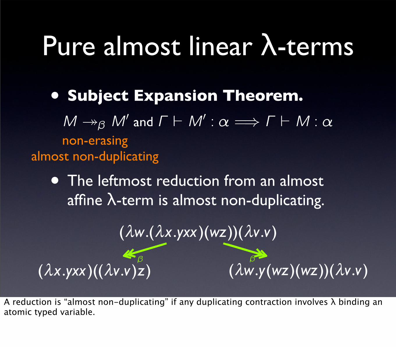
Pure almost linear λ-terms
• The principal typing of an almost affine λ-term is negatively non-duplicated.
• If M has a negatively non-duplicated typing, it is βη-equal to an almost affine λ-term.
Aoto 1999
M = λuv .∃(e→t )→t (λy .∧ t→t→t (uy )(vy ))
Almost linear = almost affine + λI“Negatively non-duplicated” means that there is at most one negative occurrence of any atomic type.

Pure almost linear λ-terms
• Coherence Theorem. All inhabitants of a negatively non-duplicated typing are βη-equal.
Aoto and Ono 1994
Pure almost linear λ-terms
• Subject Expansion Theorem.
• The leftmost reduction from an almost affine λ-term is almost non-duplicating.
non-erasingalmost non-duplicating
(λw .(λx .yxx )(wz))(λv .v )
(λw .y(wz)(wz))(λv .v ) (λx .yxx )((λv .v )z)ββ
A reduction is “almost non-duplicating” if any duplicating contraction involves λ binding an atomic typed variable.

yes!

no!
A tricky case.

yes!

• Given an input λ-term, find the most compact term graph (≈ fully collapsed form) representing it.
• This graph represents a pure almost linear λ-term.
Reduction to Datalog
The two occurrences of John are identified, but not the two occurrences of ∧.
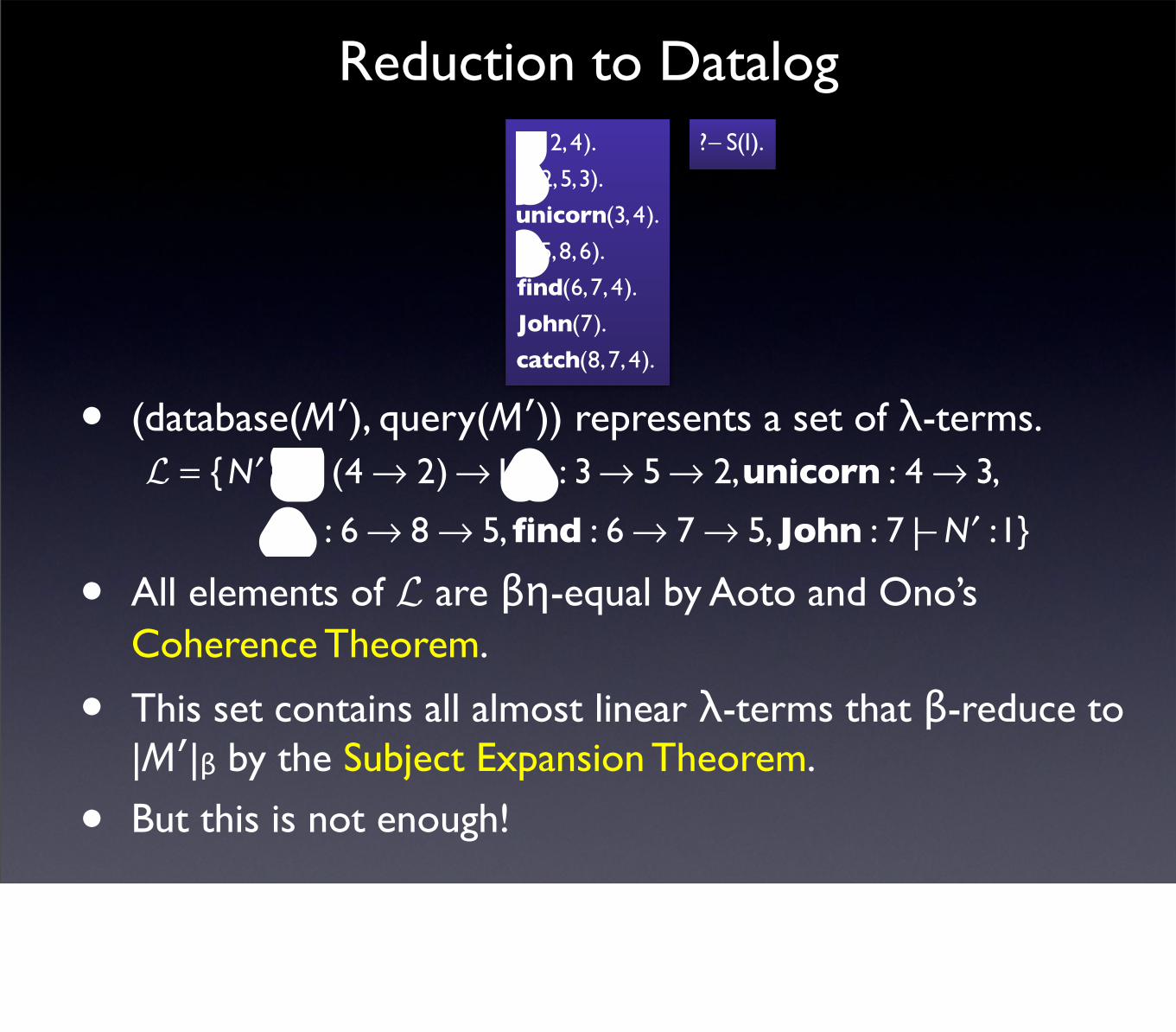
• (database(M′), query(M′)) represents a set of λ-terms.
• All elements of L are βη-equal by Aoto and Ono’s Coherence Theorem.
• This set contains all almost linear λ-terms that β-reduce to |M′|β by the Subject Expansion Theorem.
• But this is not enough!
Reduction to Datalog
L = { ′N | ∃ : (4 → 2)→1,∧1: 3→ 5→ 2,unicorn : 4 → 3,
∧2
: 6 → 8 → 5, find : 6 → 7 → 5, John : 7 |− ′N :1}
∃(1,2,4).
∧(2,5,3).
unicorn(3,4).
∧(5,8,6).
find(6,7,4).
John(7).
catch(8,7,4).
?− S(1).

• (database(M′), query(M′)) represents a set of λ-terms.
• Since M′ is the most compact almost linear λ-term such that M′θ ↠β M (where θ is the substitution that gives back the original constants), for every almost linear N such that N ↠β M, there is an N′∈ L such that N′θ = N.
Reduction to Datalog
L = { ′N | ∃ : (4 → 2)→1,∧1: 3→ 5→ 2,unicorn : 4 → 3,
∧2
: 6 → 8 → 5, find : 6 → 7 → 5, John : 7 |− ′N :1}
∃(1,2,4).
∧(2,5,3).
unicorn(3,4).
∧(5,8,6).
find(6,7,4).
John(7).
catch(8,7,4).
?− S(1).


A Datalog derivation tree determines a grammar derivation plus a typing of the associated λ-term.


Limitations

Regular sets as input
• For a linear grammar G, (database(A), query(A)) representing a finite (string or tree) automaton can be used with program(G).

Regular sets as input
• For a tree generating almost linear grammar G, (database(A), query(A)) representing a deterministic bottom-up finite tree automaton A can be used with program(G).
- PMCFG recognition via PMRTG
- generation from regular sets as underspecified representations