Special Issue Article

Advances in Mechanical Engineering2016, Vol. 8(10) 1–11� The Author(s) 2016DOI: 10.1177/1687814016671447aime.sagepub.com

Structural reliability analysis ofmultiple limit state functions usingmulti-input multi-output supportvector machine

Hong-Shuang Li1, An-Long Zhao1 and Kong Fah Tee2

AbstractSelecting and using an appropriate structural reliability method is critical for the success of structural reliability analysisand reliability-based design optimization. However, most of existing structural reliability methods are developed anddesigned for a single limit state function and few methods can be used to simultaneously handle multiple limit state func-tions in a structural system when the failure probability of each limit state function is of interest, for example, in areliability-based design optimization loop. This article presents a new method for structural reliability analysis with multi-ple limit state functions using support vector machine technique. A sole support vector machine surrogate model for alllimit state functions is constructed by a multi-input multi-output support vector machine algorithm. Furthermore, thismulti-input multi-output support vector machine surrogate model for all limit state functions is only trained from onedata set with one calculation process, instead of constructing a series of standard support vector machine models whichhas one output only. Combining the multi-input multi-output support vector machine surrogate model with directMonte Carlo simulation, the failure probability of the structural system as well as the failure probability of each limit statefunction corresponding to a failure mode in the structural system can be estimated. Two examples are used to demon-strate the accuracy and efficiency of the presented method.

KeywordsStructural reliability, multi-input multi-output support vector machine, multiple limit state functions, Latin hypercubesampling, Monte Carlo simulation

Date received: 15 June 2016; accepted: 6 September 2016

Academic Editor: Yongming Liu

Introduction

During the past few decades, structural reliability meth-ods have been gained increasing interest for rationaltreatment of the uncertainties in engineering structures.Despite the structural reliability community hasachieved many advanced development on the theoreti-cal research, serious computational obstacles arisewhen involving practical problems. For example, itusually involves the reliability assessment of multiplelimit state functions (LSFs) in reliability-based designoptimization (RBDO) of a structure, and many

structures may have multiple failure modes which resultin multiple LSFs. A structural reliability method capa-ble of dealing multiple LSFs from the same system with

1College of Aerospace Engineering, Nanjing University of Aeronautics

and Astronautics, Nanjing, China2Department of Engineering Science, University of Greenwich, London,

UK

Corresponding author:

Hong-Shuang Li, College of Aerospace Engineering, Nanjing University of

Aeronautics and Astronautics, Nanjing 210016, China.

Email: hongshuangli@nuaa.edu.cn

Creative Commons CC-BY: This article is distributed under the terms of the Creative Commons Attribution 3.0 License

(http://www.creativecommons.org/licenses/by/3.0/) which permits any use, reproduction and distribution of the work without

further permission provided the original work is attributed as specified on the SAGE and Open Access pages (https://us.sagepub.com/en-us/nam/

open-access-at-sage).

a single run is more preferable for RBDO problemsand multiple-LSF problems. When one examines theexisting structural reliability methods, an importancefact is found that most of them are developed for a sin-gle LSF, for example, the most commonly used first-order reliability method (FORM) and second-orderreliability method (SORM).1–5 Although one mayrepeat to apply the existing structural reliability meth-ods on each LSF, the computational and developmenteffort cannot meet the demands in many practicalcases. Therefore, the study of structural reliabilitymethods which can deal with multiple LSFs simultane-ously has progressively attracted attention recently,especially on computer-based simulation methods. Dueto its excellent universality, direct Monte Carlo simula-tion (MCS) is suitable for a problem with multipleLSFs. However, the huge computational effort forsmall reliability level hinders its applications, just likethe situation for a single LSF.6–8 Based on subset simu-lation (SS),6 Hsu and Ching9 developed a simulationalgorithm for the failure probabilities of multiple LSFs.In their algorithm, a principle variable is proposed tocorrelate with all LSFs of interest and drive the simula-tion to gradually approach the multiple failure regions.However, it is a non-trivial task for the determinationof a proper principle variable. Li et al.10 proposed ageneralized SS to use unified intermediate events toresolve the sorting difficulty in the original one. In gen-eral, the generalized SS is much easy to carry out areliability analysis of multiple LSFs simultaneously,compared with Hsu and Ching’s method. Like MCS,SS is also very time-consuming when structural analy-ses involve large numerical models, for example, finiteelement models.11

In practical problems, LSFs are established basedon certain structural failure mechanism, for example,stress, displacement, and fatigue, and do not have ana-lytical expressions. Furthermore, the failure regionsusually possess complicated geometry and boundaries.In order to reduce the computational effort of struc-tural reliability analysis, surrogate models, for example,response surface method (RSM),12–20 artificial neuralnetworks (ANNs),21–24 and support vector machine(SVM),25–29are generally suggested to approximate theactual LSF in a structural reliability problem. RSMmay be the most popular methods among them. It aimsto fit an LSF around the so-called design point as nearas possible. However, its approximate precision isgreatly influenced by an LSF’s complexity, polynomialform and order, and location of supporting points.11,21

It has been proved that even a response surface withaccuracy as one wish may produce an erroneous esti-mation for failure probability.30 Moreover, RSM is notapplicable to the situation of multiple LSFs. ANN isone of the popular alternatives to RSM. Various kindsof ANNs may estimate the failure probabilities of

multiple LSFs simultaneously with the aid of its highparallelism. However, in the case of a small number oftraining samples, the estimated results are greatly influ-enced by the initial parameter setting, and the trainingprocess is easy to fall into local optimum because ANNis mainly based on the principle of empirical risk mini-mization (ERM).31–33 Recently, Chojaczyk et al.22 pro-vided a comprehensive review on the application ofANN in structural reliability analysis.

SVM was first proposed by Cortes and Vapnik31 in1995, which reveals many unique advantages in patternrecognition with small samples, nonlinear and highdimensions. It was further extended for nonlinearregression by Vapnik.32,33 From the point of view ofstatistical learning theory, SVM has several advantagesover RSM and ANN for the approximation of anLSF.25 SVM adopts the structural risk minimization(SRM) principle rather than the ERM principle so thatSVM has better generalization ability. In addition,there is no local optimal issue when searching the algo-rithm parameters in an SVM. Due to its superior per-formance, SVMs have been developed to combine withconventional structural reliability methods to establishnew structural reliability methods. Those advantagesmentioned previously can inhere in the structural relia-bility methods based on various SVMs. Hurtado andAlvarez25 proposed an interesting method composed ofSVM and stochastic finite element method to deal withstructural reliability analysis by means of regarding theproblem of structural reliability analysis as a patternrecognition problem. By combining SVM with FORMand MCS, the two approaches, SVM-based FORMand SVM-based MCS, were proposed by Li et al.26 forstructural reliability analysis. Guo and Bai27 suggesteda method that combines the least square SVM withMCS. It indicates the method based on the least squareSVM is superior to the method based on traditionalSVM. Dai et al.28 developed a SVM-based importancesampling to perform structural reliability analysis, inwhich SVM is used to construct the sampling densityfor the optimal important sampling density to reducethe number of training samples. Jiang et al.29 paid aspecial attention to generating uniform support vectorfor the SVMs’ application on structural reliabilityanalysis.

Although SVMs have been widely used in reliabilitycommunity, a series of traditional SVM models whichonly have one output are needed to be constructedwhen dealing with multiple LSFs simultaneously.34

This strategy may have very low computational effi-ciency, because both actual LSFs and their surrogatemodels are required to be called for a large number oftimes during surrogate model construction and reliabil-ity estimation.

As an alternative to the traditional SVMs, multiple-input multiple-output SVMs (MIMO-SVMs)35–38 are

2 Advances in Mechanical Engineering

good choice since they can model the multiple-inputmultiple-output relationship between the input randomvariables and the multiple failure modes in a structuralsystem and have been applied in many engineering andscience fields. The newly developed multiple-task least-squares SVMs (MTLS-SVMs) which is proposed byXu et al.35,36 aims for establishing a surrogate modelbetween input parameters and multiple outputs formultiple classification and regression problems. Thisarticle presents a new method for structural reliabilityanalysis of multiple LSFs, which utilizes the recentlydeveloped MTLS-SVM. To our best knowledge, this isthe first attempt to employ MTLS-SVM for structuralreliability analysis of multiple LSFs. A new randomsampling method, combining the Latin hypercube sam-pling (LHS) and uniform sampling (US), is also devel-oped to generate the training data (supporting points)set with a good coverage of the input random space.Then, the MTLS-SVM is trained to be a single surro-gate model for all LSFs in the problem of interest.Finally, based on the trained MTLS-SVM model, MCSis employed to estimate the failure probabilities of allLSFs simultaneously. The computational efficiency andaccuracy of the presented method are also studied inthis article.

SVM technique

In this section, some basic concepts of SVM are brieflyreviewed. More details of SVM can be referred toVapnik.32 It is well known that SVM is a statisticallearning algorithm based on SRM, which can be usedfor classification and regression problems. Here, wefocus on the regression problems, that is, function fit-ting problems.

Considering a training data set

S = x1, y1ð Þ, x2, y2ð Þ, . . . , xl, ylð Þf g, xi 2 Rn, yi 2 R

ð1Þ

where l is sample size, xi is the input parameters, and yis the scalar output, respectively.

The nonlinear relationship between the inputs andoutput can be described by a regression functionobtained from SVM theory

f xð Þ=u xð ÞTw+ b=Xxi2SV

ai � a�i� �

K xi, xj

� �+ b ð2Þ

where f (x) is the regression function, u(x) is a mappingfunction for a higher dimensional Hilbert space, w isthe control parameter of the hyperplane in the Hilbertspace, ai and a�i are the Lagrange multipliers, andK(xi, xj) is the kernel function which meets the Mercercondition,32,33 respectively. Furthermore, a small por-tion of samples in the whole training data set have non-

zero ai and a�i . These samples, which are used to con-struct a regression function rather than the whole dataset, are called support vectors (SVs). The values of ai,a�i , and b can be obtained by minimizing the followingdual objective function with constraints

min1

2

Xl

i, j= 1

ai � a�i� �

aj � a�j

� �K xi, xj

� �

+ eXl

i= 1

ai +a�i� �

�Xl

i= 1

yi a�i � ai

� �

s:t:Xl

i= 1

a�i � ai

� �= 0, 0�ai, a�i � c

i, j= 1, 2, . . . , lð Þ

ð3Þ

where c is a regularization parameter used to measurethe complexity and the loss of compromise, and e is alinear insensitive loss function. According to theKarush–Kuhn–Tucker (KKT) complementary condi-tions, equation (3) has a global optimal solutionbecause SVM converts a regression problem into aquadratic optimization problem.

The kernel function K(xi, xj) is one of key compo-nents of SVM. In SVM, a nonlinear problem in theinput space is converted into a linear problem in ahigh-dimensional feature space. The inner product inthe feature space will be replaced by the kernel functionK(xi, xj) which meets the Mercer condition. Therefore,the expression of nonlinear transformation will not beneeded any more. Several kinds of commonly used ker-nel functions are given below: (1) liner kernel functionK(xi, xj)= hxi, xji; (2) polynomial kernel functionK(xi, xj)= (hxi, xji+ 1)q; (3) radial basis kernel func-tion K(xi, xj)= exp (� xi � xj

�� ��2=s2); and (4) sigmoid

kernel function K(xi, xj)= tanh (vhxi, xji+ a).

The least square MIMO-SVM

The above-mentioned SVM technique is able to beapplied to a system with a single output only. Thus, itcannot be used for dealing with a complex system withmultiple outputs, for example, the demand of dealingwith multiple LSFs in an RBDO problem as in thisstudy. To overcome this issue, various MIMO-SVMtechniques have been proposed to meet this demand.35–38

In this article, a MTLS-SVM35,36 is employed to buildup a single surrogate model which can approximate mul-tiple LSFs.

Considering a system has m outputs, the trainingsample size is l. The training data set in equation (1)becomes as

S = xi, yið Þli= 1

n o, xi 2 Rn, yi 2 Rm

i= 1, 2, . . . , lð4Þ

Li et al. 3

where n is the dimension of input parameters.According to the Hierarchical Bayesian,39,40 the controlparameter wi can be expressed as wi =w0 + vi, whichreflects the relationship and difference among the out-puts. Here, the mean vector w0 is small when the out-put quantities are very different to each other,otherwise the vector is small. Therefore, w0 embodiesthe common information among the outputs, and vi

embodies the information of the specialty of the ithoutput.

To solve the regression problem of multiple outputssystem, MIMO-SVM determines w0, vi, and bi simulta-neously by minimizing the following objective functionwith constraints

min1

2wT

0w0 +1

2

l

m

Xm

i= 1

vTi vi + c

Xm

i= 1

jTi ji

s:t: yi =ZTi w0 + við Þ+ bi 1l + ji

i= 1, 2, . . . , mð Þ

ð5Þ

where l and c are two positive real regularized para-meters, 1l =(1, . . . , 1)T 2 Rl, Zi =(f(xi, 1),f(xi, 2), . . . ,f(xi, l)), ji =(ji, 1, ji, 2, . . . , ji, l)

T.Pm

i= 1 jTi ji is a quad-ratic loss function instead of the linear insensitive lossfunction e in section ‘‘SVM technique.’’

The Lagrange function is introduced to solve theoptimization problem in equation (6)

L w0, vi, b, ji,aið Þ= 1

2wT

0w0 +1

2

l

m

Xm

i= 1

vTi vi + cXm

i= 1

jTi ji

�Xm

i= 1

aTi ZT

i w0 + við Þ+ bi 1l + ji � yi

� �

i= 1, 2, . . . , mð Þ ð6Þ

where ai =(ai, 1,ai, 2, . . . ,ai, l)T are the Lagrange multi-

pliers. The KKT conditions for equation (6) are givenby

∂L

∂w0

= 0,∂L

∂vi

= 0,∂L

∂bi

= 0,∂L

∂ji

= 0,

∂L

∂ai

= 0 i= 1, 2, . . . , mð Þ ð7Þ

The following linear equations are obtained

w0 =Zavi =

mlZiaiPm

i= 1

ai = 0

ai = 2cji

yi =ZTi w0 + við Þ+ bi 1l + ji

8>>>>>><>>>>>>:

i= 1, 2, . . . , m

ð8Þ

where Z=(Z1,Z2, . . . ,Zm), and a=(aT1 , a

T2 , . . . ,

aTm)

T. Then, one has a matrix equation

0m 3 m OT

O H

� �� b

a

� �=

0m

y

� �ð9Þ

where O=(1l1 , 1l2 , . . . , 1lm ) is a block diagonal matrix,the positive definite matrix H=ZTZ+(1=2c)Il +(m=l)B, Il is unitary matrix, and B=(K1,K2, . . . ,Km)is a block diagonal matrix with the element Ki =ZT

i Zi,respectively. Let the solution to equation (9) bea�=(a�T1 , a�T2 , . . . , a�Tm )T and b=(b�1, b�2, . . . , b�m)

T.Then, the regression estimate functions can beexpressed as

fi xð Þ=f xð ÞT w�0 + v�i� �

+ b�i

=f xð ÞT Za�+m

lZia

�i

� �+ b�i

=Xm

i9 = 1

Xl

j= 1

a�i9, jK xi9, j, x� �

+m

l

Xl

j= 1

a�i9, jK xi, j, x� �

+b�i

i= 1, 2, . . . ,m

ð10Þ

More details about the MIMO-SVM algorithm canbe seen in Xu et al.35,36

Structural reliability analysis based onMIMO-SVM

It is well known that LSF is the foundation of the struc-tural reliability analysis. In this article, MIMO-SVM isused to construct a single surrogate model of all multi-ple LSFs through a single run. On the basis of this sur-rogate model, MCS is then employed to calculate thefailure probabilities of all LSFs simultaneously. Thissection starts with the development of a new randomsampling method. Then, the implementation procedureof the presented method is provided.

The generation of training samples

For most of surrogate model methods, the trainingsample size and position are critical to construct anappreciate surrogate model which can meet the require-ments of efficiency and accuracy. Although SVM tech-niques possess a good generalization performancecompared with other machine learning algorithms, asmall number of training samples is always preferableto construct a high accuracy surrogate model. From ageneral sense, MCS may be used to generate a trainingdata set. However, random samples, generated accord-ing to the underlying probability distribution of ran-dom variables in MCS, usually cluster in a localdomain and cannot completely represent the inputspace well. Moreover, MCS is not easy to obtain failuresamples which represent structural characteristics in thefailure domain, especially for small failure probabilitylevels. The training data set without failure samples still

4 Advances in Mechanical Engineering

may be used to train a surrogate model. However, itsprecision and generalization cannot be guaranteed.Thus, MCS is not suitable to generate the training dataset for the purpose of training a proper surrogatemodel.

An LHS technique41,42 is employed to generate thetraining samples in this article. In essence, LHS is akind of multi-dimensional stratified sampling methodin order to obtain a good coverage of input space andreduce the statistical uncertainty associated with MCS.Suppose that N training samples are required, the accu-mulative probability interval [0,1] of a random variableis divided into N non-overlapping subintervals

ui =u

N+

i� 1

Ni� 1

N\ui\

i

N

8><>: i= 1, 2, . . . ,N ð11Þ

where u is a uniform random number in the interval[0,1] and ui is the random number in the ith subinterval(i� 1=N)\ui\(i=N ), respectively. Then, the samplingin each subinterval is isoprobable and independent.This strategy avoids the large number of random sam-pling using MCS. The median LHS is adopted in thisarticle, that is, u= 0:5. Let u=(u1, u2, . . . , uN )

T be arandom set of ui. The sampling point xi can be obtainedaccording to the inverse cumulative distribution func-tion of their marginal distributions

xi =F�1j uið Þ i= 1, 2, . . . , N ð12Þ

where F�1(ui) is the inverse cumulative distributionfunction of the jth random variable. Without loss ofgenerality, the input random variables are assumed tobe independent. Even the input random variables aredependent, the above procedure still can be used togenerate the training samples since the correlationamong the input random variables is not needed to beconsidered at this stage. The above procedure can beeasily extended to a problem of n-dimension. Suppose,the N sampling points are needed to be generated in ann-dimensional input space, first, the n-dimensionalinput space is split into Nn equal-sized hypercubes.Then in each hypercube, a random sample is generated.It should be pointed out that the N hypercubes need tobe satisfied by the following requirement: only onehypercube can be chosen in any direction parallel withany of the axes.

If the associated failure probability of an LSF is toosmall, the training data set generated by LHS techniquemay not include any failure points. In order to addressthis issue, an improved sampling method, combiningLHS technique and uniform sampling (US), is proposedto provide a good coverage of the whole input random

space. This new method is denoted as LHS + US inthis article. After generating ui by LHS technique, xi isobtained through a uniform mapping, that is, ui ismapped from the interval [0,1] to a compatible interval½mj � ksj,mj + ksj�, instead of the complex inversemanipulation. Here, parameter k is a constant, which isused to describe the coverage of the training data set.Therefore, the selection of k should guarantee that thereare enough failure points in the training data set. Anempirical experience is that the value of k falls into aninterval [3, 9] because the maximum allowable failureprobability of a practical structure is less than 1023.Here, a system with two LSFs is used to show the effectof parameter k. These two LSFs are given by

g1 xð Þ= 2� x2 + exp �0:1x1ð Þ2 + 0:2x1ð Þ4

g2 xð Þ= 4:5� x1x2

ð13Þ

where x1 and x2 are two standard normal variables.Figure 1 shows 20 samples generated by LHS and

LHS + US separately. Figure 1(a) presents the samplesobtained by LHS technique. It can be seen that these 20samples do not contain any failure samples and thencannot cover the input space well. Figure 1(b)–(d)shows the training samples obtained by LHS + US. Itcan be seen that the higher the value of k, the more thefailure points will be generated and the better the cover-age of random samples.

To select a proper value for k, a practical way is tostart with k=6 and check the percentage of failuresamples. If this value is larger than 20%, the generationof training samples can be terminated. Otherwise, alarger value of k needs to be set.

Procedure of the presented method

Considering a structural system with m LSFs

g1 Xð Þ= g1 x1, x2, . . . , xkð Þ...

gm Xð Þ= g1 x1, x2, . . . , xkð Þ

8><>: ð14Þ

The general procedure of the presented method isgiven below. First, the training samples required to con-struct a surrogate model are generated by LHS + US.Then, in order to select an appropriate kernel function,the corresponding parameters are determined by a grid-search method43 according to the selected kernel functionand the training samples. After that, the sole surrogatemodel of all m LSFs is trained, based on the above infor-mation and the sampling algorithm presented in section‘‘The generation of training samples.’’ Finally, MCS isemployed to estimate the failure probabilities of all mLSFs based on the MIMO-SVM surrogate model. Forthe jth LSF, its failure probability is estimated as

Li et al. 5

Pfj =P gj Xð Þ\0� �

’nj

N, j= 1, 2, . . . ,m ð15Þ

where gj(X) is the jth LSF from the trained surrogatemodel, N is the total number of samples or simulationsin MCS, and nj is the total number of failure samplesfor LSF gj(X), respectively. The above procedure issummarized in Figure 2.

Numerical examples

Two examples are used to illustrate the accuracy andefficiency of the presented method in this section,including one numerical example and one engineeringproblem. Example 1 is a two-dimensional structuralsystem with four LSFs. It gives a visual representationof the effect of MIMO-SVM and the impact of trainingsample size and kernel function. Example 2 has 11seven-dimensional LSFs, which is used to demonstratethe capacity of dealing with multiple LSFs by MIMO-SVM.

Example 1

Considering a reliability analysis problem of a struc-tural system with 4 two-dimensional LSFs, it was takenand modified from Waarts.11 System failure is definedas gs(x)= minfg1(x), g2(x), g3(x), g4(x)g, and all fourLSFs are given by

g1 xð Þ= 0:1 x1 � x2ð Þ2 � x1 + x2ffiffiffi2p + 3

g2 xð Þ= x1 � x2 + 3:5ffiffiffi2p

g3 xð Þ= 0:1 x1 � x2ð Þ2 + x1 + x2ffiffiffi2p + 3

g4 xð Þ= � x1 + x2 + 3:5ffiffiffi2p

ð16Þ

where x1 and x2 are independent standard normal ran-dom variables. Both the failure probability of systemand the failure probability of each LSF are requiredto be estimated simultaneously. In this problem,LHS + US is employed to generate random samples

Figure 1. Random sampling by LHS and LHS + US: (a) LHS, (b)LHS + US with k = 3, (c) LHS + US with k = 6, and (d)LHS + US with k = 9.

6 Advances in Mechanical Engineering

with k=8, and sample size is chosen as 10 and 20 forillustrative purpose. The quadratic and cubic polyno-mial kernel functions and the radial basis kernel func-tion are used for training MIMO-SVM surrogatemodel. Figure 3 shows the fitting results with differentkernel functions and different sample size. MCS with106 samples is employed to estimate the failure prob-abilities of interest, based on the trained MIMO-SVMmodel. The failure probabilities of LSFs are summar-ized in Table 1.

It can be seen from Figure 3 that the MIMO-SVMmodel possesses highly approximated precision whenan appropriate number of failure samples is included inthe training data set. However, the sample size seems tohave a small influence on the approximated precisionof the MIMO-SVM model when it is larger than 10.For this example, the MIMO-SVM models with differ-ent kernel functions may have similar precision.The simulation results from MCS (the second row inTable 1) are considered as ‘‘actual’’ ones, and they areused to compare to the computational results obtainedby the proposed method. Table 1 indicates the pre-sented method is as accurate as MCS. It is more effi-cient than the latter because it only needs a smallnumber of training samples.

It is worth noting that the MIMO-SVM model isconstructed only by one training run, while the number

of training runs of a single-output SVM is identicalwith the number of LSFs in a system. Furthermore, asingle-output SVM may require a different trainingdata set for each LSF in the system. In this example,the MIMO-SVM model and the single-output SVMmodel have very similar precision, while the formerneeds as less as 10 training samples and the latter needs40 training samples.

Example 2

As shown in Figure 4, a speed reducer44 has beendesigned to minimize its weight. There are 11 prob-abilistic constraints, and they represent bending, con-tact stress, longitudinal displacement, stress of theshaft, and geometry constraints. This design optimi-zation problem has seven design variables: gear width(x1), teeth module (x2), number of teeth in the pinion(x3), distance between bearings (x4, x5), and axis dia-meters (x6 and x7). Input random variables x1–x7 aremutually independent normal random variables witha standard deviation of 0.005. The objective functionand the formulae of the probabilistic optimization aregiven by

find x= x1, . . . , x7ð Þmin f xð Þ= 0:7854x1x2

2

3:3333x23 + 14:0934x3 � 43:0934

� �� 1:508x1 x2

6 + x27

� �+ 7:477 x3

6 + x37

� �+

0:7854 x4x26 + x5x2

7

� �s:t: Pr gi xð Þ.0½ � � 1� F bið Þ, i= 1, . . . , 11

ð17Þ

and

Figure 2. Flowchart of the presented method.

Table 1. The failure probabilities of all LSFs in Example1 (3 10–3).

LSFs g1(x) g2(x) g3(x) g4(x) gs(x)

MCS 0.853 0.229 0.879 0.240 2.22Single SVM 0.904 0.204 0.852 0.256 2.22M-poly-2 (10) 0.904 0.204 0.852 0.256 2.22M-poly-3 (10) 0.876 0.246 0.866 0.224 2.21M-poly-2 (20) 0.904 0.204 0.852 0.256 2.22M-RBF (10) 0.976 0.212 0.924 0.260 2.37M-RBF (20) 0.904 0.204 0.848 0.256 2.21

LSF: limit state function; MCS: Monte Carlo simulation; SVM: support

vector machine; RBF: radial basis function; MIMO-SVM: multi-input

multi-output support vector machine.

M is MIMO-SVM.

The numbers in the parentheses are the sample size.

Li et al. 7

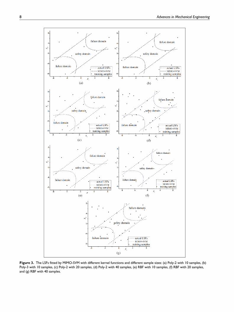
Figure 3. The LSFs fitted by MIMO-SVM with different kernel functions and different sample sizes: (a) Poly-2 with 10 samples, (b)Poly-3 with 10 samples, (c) Poly-2 with 20 samples, (d) Poly-2 with 40 samples, (e) RBF with 10 samples, (f) RBF with 20 samples,and (g) RBF with 40 samples.

8 Advances in Mechanical Engineering

g1 xð Þ= 27

x1x22x3

� 1, g2 xð Þ= 397:5

x1x22x2

3

� 1

g3 xð Þ= 1:93x34

x2x3x46

� 1, g4 xð Þ= 1:93x35

x2x3x47

� 1

g5 xð Þ=

ffiffiffiffiffiffiffiffiffiffiffiffiffiffiffiffiffiffiffiffiffiffiffiffiffiffiffiffiffiffiffiffiffiffiffiffiffiffiffiffiffiffiffiffiffiffiffiffiffiffiffiffiffiffiffiffiffiffiffi745x4= x2x3ð Þð Þ2 + 16:9 3 106

q0:1x3

6

� 1100

g6 xð Þ=

ffiffiffiffiffiffiffiffiffiffiffiffiffiffiffiffiffiffiffiffiffiffiffiffiffiffiffiffiffiffiffiffiffiffiffiffiffiffiffiffiffiffiffiffiffiffiffiffiffiffiffiffiffiffiffiffiffiffiffiffiffi745x5= x2x3ð Þð Þ2 + 157:5 3 106

q0:1x3

7

� 850

g7 xð Þ= x2x3 � 40, g8 xð Þ= 5� x1

x2

g9 xð Þ= x1

x2

� 12, g10 xð Þ= 1:5x6 + 1:9

x4

� 1,

g11 xð Þ= 1:1x7 + 1:9

x5

� 1

b1 = � � �b11 = 3:0

2:6� x1� 3:6, 0:7� x2� 0:8, 17� x3� 28,

7:3� x4� 8:3, 7:3� x5� 8:3, 2:9� x6� 3:9,

5:0� x7� 5:5

ð18Þ

It is obvious that all these 11 probabilistic con-straints are required to be estimated in each iterationduring the optimization process regardless of the usageof a double-loop or a single-loop optimization algo-rithm. Here, this study focuses on how to solve 11probabilistic constraints simultaneously based on thepresented method to reduce the total computationalcost. Table 2 summarizes three groups of optimizationresults reported in the literature,44 and these optimiza-tion results are selected to perform our illustration.

In this numerical example, 10 training samples aregenerated by LHS. Radial basis kernel function is cho-sen and the corresponding parameters are determinedby grid-search method. The single MIMO-SVM surro-gate model is trained according to the above informa-tion. Then, based on the trained MIMO-SVM model,MCS with 105 samples is employed to estimate the fail-ure probabilities of all 11 LSFs. In this article, the fail-ure probabilities of all 11 probabilistic constraints forthe three optimization cases are verified, that is, deter-ministic optimum, performance measure approach(PMA), and PMA + envelope function.44 The compu-tational results are summarized in Table 3.

Similar to Example 1, a single MIMO-SVM surro-gate model is constructed for all 11 LSFs, while 11SVM surrogate models with one output are needed tobe constructed in a traditional way. The training

Figure 4. Schematic speed reducer configuration.

Table 2. The optimization results given by Lee and Lee.44

Optimizationmethod

Objectivefunction

Design variables

Deterministic 2992 (3.50, 0.70, 17.0, 7.30, 7.72,3.35, 5.29)

PMA 3037 (3.60, 0.70, 17.8, 7.30, 7.79,3.40, 5.34)

PMA+ envelopefunction

3100 (3.60, 0.70, 17.2, 8.30, 8.30,3.58, 5.45)

Table 3. The failure probabilities of all LSFs in Example 2.

LSF Deterministic PMA PMA + envelope function

MCS MIMO-SVM MCS MIMO-SVM MCS MIMO-SVM

g1(x) 0.0000 0.0000 0.0000 0.0000 0.0000 0.0000g2(x) 0.0000 0.0000 0.0000 0.0000 0.0000 0.0000g3(x) 0.0000 0.0000 0.0000 0.0000 0.0000 0.0000g4(x) 0.0000 0.0000 0.0000 0.0000 0.0000 0.0000g5(x) 0.0923 0.0908 0.0000 0.0000 0.0000 0.0000g6(x) 0.1763 0.1768 0.0000 0.0000 0.0000 0.0000g7(x) 0.0000 0.0000 0.0000 0.0000 0.0000 0.0000g8(x) 0.4999 0.4978 4.5100 3 1025 3.700 3 1025 4.3000 3 1025 4.6 3 1025

g9(x) 0.0000 0.0000 0.0000 0.0000 0.0000 0.0000g10(x) 0.0000 0.0000 0.0000 0.0000 0.0000 0.0000g11(x) 0.4667 0.4668 0.0157 0.0154 0.0000 0.0000

LSF: limit state function; MCS: Monte Carlo simulation; MIMO-SVM: multiple-input multiple-output SVM.

Li et al. 9

sample size is only 10 for the presented MIMO-SVMsurrogate model, while at most 110 samples may beneeded when using a single-output SVM model. It canbe seen from Table 3 that the computational resultsobtained by the presented MIMO-SVM surrogatemodel with MCS are very close to those obtaineddirectly by MCS. This indicates that the presentedMIMO-SVM model has high accuracy under the con-dition of small number of samples and moderatedimensions.

Conclusion

It is well known that most of traditional structuralreliability methods cannot be applied to deal with mul-tiple LSFs simultaneously, when the failure probabilityof each LSF is of interest. A new structural reliabilitymethod using MIMO-SVM is presented to handle mul-tiple LSFs for this issue which may arise in an RBDOproblem and/or a problem with multiple failure modes.The main idea of the presented method is to constructa single surrogate model for all multiple LSFs usingMIMO-SVM because all LSFs share the commoninput parameters and model (numerical or physicalone). In order to obtain a good coverage of input para-meter space, LHS and LHS + US are proposed togenerate a training data set with a portion of failuresamples. Finally, the failure probabilities of all LSFsare estimated by MCS based on the trained MIMO-SVM surrogate model. The most attractive advantagesof this presented method are that all LSFs are approxi-mated only using one training data set and the trainingoperation is only run one time. These will be benefitedfor the estimation of probabilistic constraints in RBDOand structural reliability analysis with multiple failuremodes. Numerical examples indicate that that the pre-sented method needs a small amount of computationalcost to achieve an accurate reliability analysis. Thus, itis suitable for RBDO with multiple probabilistic con-straints and multiple modes reliability analysis.

A limitation of this study is the passive way of gen-eration of training samples. Future work will involvecombining the active learning techniques and MIMO-SVM to further reduce the computational cost andthen apply it in practical RBDO.

Declaration of conflicting interests

The author(s) declared no potential conflicts of interest withrespect to the research, authorship, and/or publication of thisarticle.

Funding

The author(s) disclosed receipt of the following financial sup-port for the research, authorship, and/or publication of this

article: The authors are grateful for the supports by theNational Science Foundation of China (Grant No. U1533109and 11102084), Fundamental Research Funds for the CentralUniversities (Grant No. NS2015007), and a Project Fundedby the Priority Academic Program Development of JiangsuHigher Education Institutions.

References

1. Hasofer AM and Lind NC. An exact and invariant first

order reliability format. J Eng Mech 1974; 100: 111–121.2. Zhao YG and Ono T. A general procedure for first/sec-

ond-order reliability method (FORM/SORM). Struct

Saf 1999; 21: 95–112.3. Rackwitz R. Reliability analysis—a review and some per-

spectives. Struct Saf 2001; 23: 365–395.4. Rackwitz R and Flessler B. Structural reliability under

combined random load sequences. Comput Struct 1978;

9: 489–494.5. Tvedt L. Distribution of quadratic forms in normal

space—application to structural reliability. J Eng Mech

1990; 116: 1183–1197.6. Au SK and Beck JL. Estimation of small failure prob-

abilities in high dimensions by subset simulation. Proba-

bilist Eng Mech 2001; 16: 263–277.7. Ditlevsen O and Madsen HO. Structural reliability meth-

ods. Hoboken, NJ: John Wiley & Sons, 1996.8. Bucher C. Computational analysis of randomness in struc-

tural mechanics. London: CRC Press, 2009.9. Hsu WC and Ching J. Evaluating small failure probabil-

ities of multiple limit states by parallel subset simulation.

Probabilist Eng Mech 2010; 25: 291–304.10. Li HS, Ma YZ and Cao Z. A generalized Subset Simula-

tion approach for estimating small failure probabilities of

multiple stochastic responses. Comput Struct 2015; 153:

239–251.11. Waarts PH. Structural reliability using finite element meth-

ods: an appraisal of DARS: directional adaptive response

surface sampling. Amsterdam: Delft University Press,

2000.12. Bucher CG and Bourgund U. A fast and efficient

response surface approach for structural reliability prob-

lems. Struct Saf 1990; 7: 57–66.13. Rajashekhar MR and Ellingwood BR. A new look at the

response surface approach for reliability analysis. Struct

Saf 1993; 12: 205–220.

14. Kim SH and Na SW. Response surface method using vec-

tor projected sampling points. Struct Saf 1997; 19: 3–19.15. Kaymaz I and McMahon CA. A response surface

method based on weighted regression for structural relia-

bility analysis. Probabilist Eng Mech 2005; 20: 11–17.16. Gavin HP and Yau SC. High-order limit state functions

in the response surface method for structural reliability

analysis. Struct Saf 2008; 30: 162–179.17. Li D, Chen Y, Lu W, et al. Stochastic response surface

method for reliability analysis of rock slopes involving

correlated non-normal variables. Comput Geotech 2011;

38: 58–68.18. Wang Z and Wang P. A new approach for reliability

analysis with time-variant performance characteristics.

Reliab Eng Syst Safe 2013; 115: 70–81.

10 Advances in Mechanical Engineering

19. Li HS, Lu ZZ and Qiao HW. A new high-order responsesurface method for structural reliability analysis. StructEng Mech 2010; 34: 779–799.

20. Li HS. Reliability-based design optimization via highorder response surface method. J Mech Sci Technol 2013;27: 1021–1029.

21. Deng J, Gu D, Li X, et al. Structural reliability analysisfor implicit performance functions using artificial neuralnetwork. Struct Saf 2005; 27: 25–48.

22. Chojaczyk AA, Teixeira AP, Neves LC, et al. Reviewand application of artificial neural networks models inreliability analysis of steel structures. Struct Saf 2015; 52:78–89.

23. Cheng J and Li QS. Reliability analysis of structuresusing artificial neural network based genetic algorithms.Comput Method Appl M 2008; 197: 3742–3750.

24. Cheng J, Li QS and Xiao RC. A new artificial neural

network-based response surface method for structuralreliability analysis. Probabilist Eng Mech 2008; 23: 51–63.

25. Hurtado J and Alvarez D. Classification approach forreliability analysis with stochastic finite-element model-ing. J Struct Eng 2003; 129: 1141–1149.

26. Li HS, Lu ZZ and Yue ZF. Support vector machine forstructural reliability analysis. Appl Math Mech 2006; 27:1295–1303.

27. Guo Z and Bai G. Application of least squares supportvector machine for regression to reliability analysis. Chi-nese J Aeronaut 2009; 22: 160–166.

28. Dai H, Zhang H and Wang W. A support vector density-based importance sampling for reliability assessment.Reliab Eng Syst Saf 2012; 106: 86–93.

29. Jiang Y, Luo J, Liao G, et al. An efficient method forgeneration of uniform support vector and its applicationin structural failure function fitting. Struct Saf 2015; 54:1–9.

30. Li J and Xiu D. Evaluation of failure probability via sur-rogate models. J Comput Phys 2010; 229: 8966–8980.

31. Cortes C and Vapnik V. Support-vector networks. Mach

Learn 1995; 20: 273–297.32. Vapnik VN. The nature of statistical learning theory. New

York: Springer, 1995.

33. Vapnik VN. An overview of statistical learning theory.

IEEE T Neural Networ 1999; 10: 988–999.34. Anirban B, Sylvain L and Samy M. Constrained efficient

global optimization with probabilistic support vector

machines. In: 13th AIAA/ISSMO multidisciplinary analy-

sis optimization conference, Fort Worth, TX, 13–15 Sep-

tember 2010. Reston, VA: American Institute of

Aeronautics and Astronautics.35. Xu S, An X, Qiao X, et al. Multi-output least-squares

support vector regression machines. Pattern Recogn Lett

2013; 34: 1078–1084.36. Xu S, An X, Qiao X, et al. Multi-task least-squares sup-

port vector machines. Multimed Tools Appl 2014; 71:

699–715.37. Mao W, Tian M and Yan G. Research of load identifica-

tion based on multiple-input multiple-output SVM model

selection. Proc IMechE, Part C: J Mechanical Engineering

Science 2012; 226: 1395–1409.38. Mao W, Xu J, Wang C, et al. A fast and robust model

selection algorithm for multi-input multi-output support

vector machine. Neurocomputing 2014; 130: 10–19.39. Heskes T. Empirical bayes for learning to learn. In: Pro-

ceedings of 17th international conference on machine learn-

ing, Stanford, CA, 29 June–2 July 2000, pp.367–374. San

Francisco, CA: Morgan Kaufmann Publishers.40. Arora N, Allenby GM and Ginter JL. A hierarchical

bayes model of primary and secondary demand. Market

Sci 1998; 17: 29–44.41. Stein M. Large sample properties of simulations using

Latin hypercube sampling. Technometrics 1987; 29:

143–151.42. Olsson A, Sandberg G and Dahlblom O. On Latin hyper-

cube sampling for structural reliability analysis. Struct

Saf 2003; 25: 47–68.43. Hsu CW, Chang CC and Lin CJ. A practical guide to sup-

port vector classification. Taipei, Taiwan: Department of

Computer Science, National Taiwan University, 200344. Lee JJ and Lee BC. Efficient evaluation of probabilistic

constraints using an envelope function. Eng Optimiz

2005; 37: 185–200.

Li et al. 11