advancing population ecology with integral projection...

REVIEW

Advancing population ecologywith integral projection

models: a practical guide

CoryMerow1,2*, JohanP. Dahlgren3,4, C. Jessica E.Metcalf5,6, Dylan Z. Childs7, Margaret E.K.

Evans8, Eelke Jongejans9, SydneRecord10, Mark Rees7, Roberto Salguero-G�omez11,12 and

SeanM.McMahon1

1Smithsonian Environmental ResearchCenter, 647 ConteesWharf Rd, Edgewater, MD 21307Edgewater, MD21307-0028,

USA; 2Ecology andEvolutionary Biology, University of Connecticut, Storrs, CT 06269, USA; 3Department of Ecology,

Environment and Plant Sciences, StockholmUniversity, Stockholm, Sweden; 4Department of Biology andMax-Planck

OdenseCenter on the Biodemography of Aging, University of Southern Denmark, Odense, Denmark; 5Department of Zoology,

Oxford University, Oxford, UK; 6Department of Ecology and Evolutionary Biology, PrincetonUniversity, Princeton, NJ, USA;7Department of Animal and Plant Sciences, University of Sheffield, Sheffield, UK; 8Laboratory of Tree-RingResearch and

Department of Ecology andEvolutionary Biology, University of Arizona, Tucson, AZ, USA; 9Department of Animal Ecology and

Ecophysiology, Institute forWater andWetlandResearch, RadboudUniversity Nijmegen, Nijmegen, TheNetherlands;10Harvard University, Harvard Forest, Petersham,MA, USA; 11MaxPlanck Institute for Demographic Research, Evolutionary

Demography laboratory, Rostock, Germany; and 12Centre for Biodiversity andConservation Science, University of

Queensland, St Lucia, Qld, Australia

Summary

1. Integral projection models (IPMs) use information on how an individual’s state influences its vital rates – sur-

vival, growth and reproduction – to make population projections. IPMs are constructed from regression models

predicting vital rates from state variables (e.g. size or age) and covariates (e.g. environment). By combining

regressions of vital rates, an IPM provides mechanistic insight into emergent ecological patterns such as popula-

tion dynamics, species geographic distributions or life-history strategies.

2. Here, we review important resources for building IPMs and provide a comprehensive guide, with extensive R

code, for their construction. IPMs can be applied to any stage-structured population; here, we illustrate IPMs for

a series of plant life histories of increasing complexity and biological realism, highlighting the utility of various

regression methods for capturing biological patterns. We also present case studies illustrating how IPMs can be

used to predict species’ geographic distributions and life-history strategies.

3. IPMs can represent a wide range of life histories at any desired level of biological detail. Much of the strength

of IPMs lies in the strength of regressionmodels.Many subtleties arise when scaling from vital rate regressions to

population-level patterns, so we provide a set of diagnostics and guidelines to ensure that models are biologically

plausible. Moreover, IPMs can exploit a large existing suite of analytical tools developed for matrix projection

models.

Key-words: demography, elasticity, life history, matrix projection model, population growth rate,

population projectionmodel, sensitivity, stage structure, vital rates

Introduction

Demography underpins many contemporary challenges in

ecology. From understanding species’ distributions to the fate

of biodiversity under climate change, demography links the

processes that affect individuals to population- and commu-

nity-level patterns (e.g. Adler, Ellner & Levine 2010). Integral

projection models (IPMs; Easterling, Ellner & Dixon 2000)

have emerged as a powerful tool for quantifying how the vital

rates of individuals (i.e. survival, growth and fecundity) govern

such higher-level properties, partly because they rely on the

flexibility and simplicity of regression models. IPMs provide a

mechanistic approach to understanding and linking biological

processes across scales, which permits evaluation of the biolog-

ical plausibility of models at each step of the analysis to make

robust predictions (Fig. 1).

Building IPMs typically begins by obtaining longitudinal

data describing individuals’ vital rates. The minimum data

required for an IPMconsists of two censuses of individual state

and fate (typically for estimation of survival and growth and

optionally fecundity; Appendix S1-S7). The fundamental*Correspondence author. E-mail: [email protected]

© 2013 The Authors. Methods in Ecology and Evolution © 2013 British Ecological Society

Methods in Ecology and Evolution 2014, 5, 99–110 doi: 10.1111/2041-210X.12146

building blocks of IPMs are regression models that relate the

state of an individual (e.g. size, age and location) to its vital

rates. The regressionsmay also include additional biotic or abi-

otic covariates that explain variation in vital rates beyond the

effects of individual state (Appendix S1,F; Dahlgren & Ehrl�en

2009; Adler, Ellner & Levine 2010; Dalgleish et al. 2011;

Nicol�e et al. 2011). In this way, IPMs can link observations of

an individual (Fig. 1a) to variation in vital rates among

individuals (Fig. 1b) to project population dynamics (Fig. 1c)

and emergent biological patterns such as fitness land-

scapes (Appendix S1,G) or range limits (Appendix S1,F;

Fig. 1d).

Previous work has highlighted some of the strengths of

IPMs as they compare to matrix population models (MPMs;

cf. Caswell 2001; Easterling, Ellner & Dixon 2000; Ellner &

Rees 2006; Coulson 2012; Ozgul et al. 2012). A primary differ-

ence between the two frameworks is that MPMs assume that

individuals occupy discrete stages, whereas IPMs naturally

accommodate both discrete and continuous state variables

(e.g. Childs et al. 2003; Jacquemyn, Brys & Jongejans 2010;

Yule, Miller & Rudgers 2013). For some organisms, it is natu-

ral to divide the life cycle into discrete components (e.g. insects

with particular instars), but for many others using a continu-

ous state variable is more appropriate (e.g. size). The artificial

discretization imposed by MPMs can have substantial effects

on demographic predictions because it ignores variability

among individuals within each stage (Easterling, Ellner &

Dixon 2000; Salguero G�omez & Plotkin 2010). IPMs are usu-

ally parameterized with simple regressions, whereas MPMs

typically estimate probabilities from observed transitions (but

seeMorris &Doak 2002). The vital rate regressions that under-

lie IPMs require many fewer parameters thanMPMs when fit-

ted to the same data (Ellner & Rees 2006; Ramula, Rees &

Buckley 2009). For example, rather than estimating multiple

matrix elements corresponding to stasis, shrinkage and growth

(e.g. Evans, Holsinger & Menges 2010), one can fit a single

regression for these dynamics. Such regressions can avoid over-

fitting to sparsely sampled transitions (Ramula, Rees & Buck-

ley 2009; Dahlgren, Garc�ıa & Ehrl�en 2011). Regression

modelling allows vital rates to be estimated at any value of the

state variable, which allows IPMs to describe state transitions

at very high resolution. IPM predictions are thus only as good

as the parametric assumptions and inferred transitions from

vital rate regressions.

Here, we emphasize how IPMs enable mechanistic insight

into population-level patterns by modelling the ecological fac-

tors influencing vital rates.We attempt tomake applications of

IPMs to ecology and evolution, specifically more complex

examples, more transparent. There is a growing body of work

on IPMs in animal populations (e.g. Coulson, Tuljapurkar &

Childs 2010; Ozgul et al. 2010; Coulson 2012), but here, we

focus on building IPMs for plants and note that our discussion

(a) (b)

(c) (d)

Fig. 1. Workflow for Integral projection models (IPMs). Regression is used to link demographic observations to biological inference. (a) A typical

relationship between an individual’s size in successive time intervals (g(z0|z)). (b) The expected size at time t + 1 is modelled using a quadratic

regression (red line) of size at time t. The variance ismodelled as a decreasing linear function of size at time t and illustrated with density functions for

four initial sizes. A grid is overlaid on these continuous regression functions to perform the integration (using the midpoint rule) necessary for an

IPM. (c) The discretized IPM kernel, derived from combining the growthmodel (b) with a survival and fecundity model, depicted as a heat map. (d)

Projecting IPMs across a landscape to produce a habitat suitabilitymap (Appendix S1-S7).

© 2013 The Authors. Methods in Ecology and Evolution © 2013 British Ecological Society, Methods in Ecology and Evolution, 5, 99–110

100 C. Merow et al.

readily applies to other organisms. To do this, we describe how

to build each component of an IPM for a series of increasingly

complex life histories and provide extensive R code (R Core

Team 2013) for a series of case studies in seven appendices.We

discuss diagnostic tools for IPMs and provide advice for build-

ing biologically complex IPMs.

How to build an IPM

The core of an IPM is the kernel – a function that describes

how the state of an individual at one time dictates its state and

that of its offspring at some future time. Individuals can be

characterized in terms of one or more state variables that

explain variation in vital rates; often the state variable is some

measure of size (hereafter, we simply refer to size: e.g. basal

rosette area for herbs or body length formammals).

The kernel describes how the size (z) distribution of individ-

uals at time t, nt(z), changes over one time step. Time step

length is chosen to reflect the life cycle or census interval, for

example, 1 year for long-lived organisms or seasons for short-

lived organisms. The integral of nt(z) over a size interval

I (∫I nt(z) dz) represents the number of individuals in that inter-

val. The kernel,K(z0, z),maps this size distribution at time t to

a size distribution at time t + 1 (one time step later) by

describing how individuals survive, change in state (e.g. grow

or shrink) and reproduce:

ntþ1ðz0Þ ¼ZXKðz0; zÞntðzÞdz eqn 1

where z0 indicates size at t + 1 and Ω denotes the possible

range of individual sizes (see ‘Analyzing the model’). The inte-

gral in eqn (1) performs a sum over all possible ways (survival,

growth and reproduction) of changing from size z at time t to

size z0 at time t + 1.

DECOMPOSING THE KERNEL: V ITAL RATES

To construct the kernel K(z0,z), one must first explore how

vital rates change with individual state. For most organisms,

the kernel can be split into a survival/growth kernel, P, and a

fecundity kernel, F, such that K(z0,z) = P(z0, z) + F(z0, z).The survival/growth kernel describes the probability that an

individual survives the census interval, and if so, the probabil-

ity distribution for the size it might become. The fecundity

kernel describes the number of offspring produced by repro-

ductive individuals during the census interval, and the size dis-

tribution of those new offspring. Below, we illustrate how to

construct a kernel from vital rate functions using five models

for perennial plants with life histories of increasing complexity.

In the next section (Regressions), we discuss how to

parameterize these vital rate functions using regression

models.

Example 1: A long-lived perennial plant with no seedbank

Webegin bymodelling the life history of a long-lived perennial

plant. We assume that once seeds germinate, individuals grow

until they are large enough to produce seeds, after which they

continue to reproduce until they die. Growth, fecundity and

survival are all size-dependent. In the simplest case, the

survival/growth kernel is given by P(z0, z) = s(z) g(z0|z).The survival function, s(z), depends on the size of an individ-

ual at time t and describes the probability that an individual

will survive to t + 1. The growth function, g(z0| z), describesthe probability density of size z0 that an individual of size z can

grow to during one time step, conditional on having survived.

In perennial plants, with individuals censused before seeds are

released (a ‘pre-reproductive’ census), the fecundity kernel

commonly distinguishes total seed production from all sources

of seed loss (e.g. predation, dispersal to an unsuitable habitat).

If the sources of seed loss are unknown, it is common to use an

establishment probability, pestab, as a ‘black box’ that describes

the ratio of recruits observed at t + 1 comparedwith the seeds

produced at t (Metcalf et al. 2008). The fecundity kernel can

be modelled as F(z0, z) = pflower(z) fseeds(z) pestab frecruit

size(z0), where pflower(z) is the probability of flowering as a

function of individual size z, fseeds(z) describes the number of

seeds produced as a function of individual size, and frecruit

size(z0) describes the size distribution of recruits observed at

time t + 1. Taken together, pflower(z), fseeds(z) and pestabdescribe the production of recruits, which follow the size distri-

bution frecruit size(z0).

This example exhibits a few generalities that will recur in

subsequent examples. The survival/growth and fecundity

kernels each have two components, which we term the

individual component and a size redistribution component. The

individual components are typically only functions of z (e.g.

survival, flowering probability and seed number) and describe

the number or proportion of individuals that follow the size

redistribution component. Size redistribution components are

functions of z0 (and optionally z), because they describe the sizeof individuals in the next year (e.g. growth and recruit size

distribution).

Example 2:Monocarpic perennial plant

The life cycle of monocarpic perennials is slightly more com-

plex because flowering is fatal (Rees & Rose 2002; Metcalf

et al. 2008; Rees & Ellner 2009). Distinguishing death due to

flowering from other sources of mortality is necessary because

flowering-related death has a positive effect on populations (if

a sufficient number of seeds are produced), while death before

flowering has a negative effect on populations. For a pre-repro-

ductive census, the survival/growth kernel is given by P(z0, z)=s(z)*[1 � pflower(z)]*g(z

0|z). The individual component

of P(z0, z) has two parts: one part due to flowering (pflower(z))

and one part for vegetative individuals (s(z)). Fecundity is

modelled as in Example 1.

Example 3: Perennial plant with seedbank

IPMs can also handle complex life histories using discrete

stages, such as a seedbank. In this case, we assume that all seeds

in the seedbank are demographically equivalent, regardless of


IPM guide 101

their size or age. Ramula, Rees & Buckley (2009) described an

IPM incorporating a seedbank for perennial herbs, with plants

censused before reproduction, which we illustrate here. Incor-

porating a discrete state for seed dynamics requires an addi-

tional equation to describe the number of seeds in the

seedbank. We can construct this as follows: let Bt denote the

number of seeds in the seedbank at time t, sseed surv denote the

survival probability of seeds in the seedbankover one time step,

srecruit bank denote the probability of recruiting from the seed-

bank, and srecruit direct denote the probability of skipping the

seedbank and recruiting. Then, number of seeds in the seed-

bank at t + 1 is given by:

Btþ1|{z}total seeds in seed bank

¼ Btsseed survð1�srecruit bankÞ|fflfflfflfflfflfflfflfflfflfflfflfflffl{zfflfflfflfflfflfflfflfflfflfflfflfflffl}seeds remaining in seed bank

þRX

pflowerðzÞfseedsðzÞð1�srecruit dorectÞnðzÞdz:|fflfflfflfflfflfflfflfflfflfflfflfflfflfflfflfflfflfflfflfflfflfflfflfflffl{zfflfflfflfflfflfflfflfflfflfflfflfflfflfflfflfflfflfflfflfflfflfflfflfflffl}

new seeds to seed bank

eqn 2

The term [Bt sseed surv (1 � srecruit bank)] describes the number

of seeds that will remain in the seedbank until the next year:

the total number of seeds already in the seedbank (Bt) is

reduced by those lost to mortality (sseed surv) and those lost to

recruitment (1�srecruit bank). The term [∫O pflower(z) fseeds(z)

(1�srecruit direct) nt(z) dz] describes the number of new seeds

entering the seedbank as the product of the number of new

seeds produced and the proportion that go directly to the seed-

bank (1�srecruit direct).

Equation 2 is linked to the following continuous stage

model, which describes the dynamics of the established individ-

uals:

nðz0Þ|{z}sizedestributionnextyear

¼ Btsrecruitbankfrecruitsizeðz0Þ|fflfflfflfflfflfflfflfflfflfflfflfflffl{zfflfflfflfflfflfflfflfflfflfflfflfflffl}recruitsfromseedbank

þRX½Pðz;z0 ÞþFðz;z0Þ�nðzÞdz:|fflfflfflfflfflfflfflfflfflfflfflfflfflfflffl{zfflfflfflfflfflfflfflfflfflfflfflfflfflfflffl}

transitionsincontinuousstagesandrecruitsskippingseedbank

eqn 3

The term [Bt srecruit bank frecruit size(z0)] describes the number

and size distribution of recruits germinating from the seed-

bank, that is, the total number of seeds in the seedbank (Bt)

multiplied by the proportion that recruit (srecruit bank), with the

new recruits distributed according to the size distribution

(frecruit size(z0)). The fecundity kernel inside the integral

describes the number of recruits arising from seeds that skip

the seedbank: F(z0, z)=pflower(z) fseeds(z) srecruit direct frecruit

size(z0). The function F(z0, z) differs from the two previous

examples only by the inclusion of srecruit direct, which is incorpo-

rated in the individual component and reduces the total num-

ber of seeds establishing next year by the proportion that go

into the seedbank. Any appropriate kernel for P(z0, z) can be

used. For an iteroparous herb, Ramula, Rees & Buckley

(2009) used P(z0, z) = s(z) g(z0|z), exactly as described in

Examples 1 and 2. Operationally, adding a discrete seedbank is

straightforward: it adds an extra row and column to the dis-

cretized kernel (top-most row and left-most column in Fig. 1c),

whose values are given by eqn (2) (Appendix S1,C; Hesse,

Rees &M€uller Sch€arer 2008).

Example 4: Perennial plant withmultiple discrete stages

In Example 3, seedlings were part of the continuous stage

(eqn 3), but in some cases, it is better to assign seedlings to a

separate, discrete class (St) if their vital rates have different size

dependence than larger individuals. For a model of the forest

herb Actaea spicata (Ranunculaceae; Appendix S1,F), seed-

lings were treated as a discrete class because seedling survival

was lower than expected based on their size (Dahlgren &

Ehrl�en 2009, 2011). This IPM is described with the following

three equations:

Btþ1 ¼ZXpflowerðzÞffruitðzÞfseeds=fruitntðzÞdz eqn 4

Stþ1 ¼ pestabBt eqn 5

ntþ1ðz0Þ ¼ sseed survfrecruit sizeðz0ÞSt þZXsðzÞgðz0jzÞntðzÞdz

eqn 6

A seedbank (eqn 4) accounts for the fact that under-

ground germination occurs 1 year after seed release and

above-ground recruitment 1 year later. Equation 4 differs

from the seedbank in eqn 2 in that all seeds go into the

seedbank and seeds cannot stay in the seedbank. Equa-

tion 4 also differs from eqn 2 in that the number of seeds is

modelled as a function of size in eqn 2, whereas here, the

number of fruits is modelled as a function of size (ffruit(z)),

with this multiplied by the average number of seeds per

fruit (fseeds/fruit). Seeds that survive and germinate (pestab)

become seedlings (St) for 1 year (eqn 2), and if they survive

(sseedling surv), establish the following year with the size distri-

bution given by frecruit size(z0) (eqn 6). The dynamics of

established individuals is described by eqn 6, which is

directly analogous to eqn 3.

Example 5: Perennial plant withmultiple discrete stages and

environmental covariates

Vital rate functions can readily accommodate covariates,

such as environmental conditions, that help to predict

individuals’ vital rates above and beyond the state vari-

able. For the model in Example 4, two modifications

were needed to capture population dynamics in Dahlgren

& Ehrl�en (2009, 2011); Appendix S1,F). They included

the effect of soil potassium concentration (Kconc) on

growth (replacing g(z0|z) with g(z0|z, Kconc) and the effect

of fruit predation (ppred) on the number of seeds pro-

duced per individual (replacing ffruit(z) with ffruit(z, ppred)).

This enabled them to model the temporal dynamics as a

function of changes in soil potassium concentration due

to the successional dynamics of spruce forests (details in

Appendix S1,F). The functional forms of all vital rate

functions were determined by regression and are shown in

Table 1.


102 C. Merow et al.

A wide range of life histories can be incorporated into an

IPM by including more complex discrete (e.g. seedbank and

seedlings; Appendix S1,F) or continuous stages (e.g. clonally

produced individuals; Appendix S1,B) and partitioning the

kernel into the appropriate vital rate functions. We expect that

models with multiple discrete and continuous stages represent

the future of IPMs; for example, Jacquemyn, Brys & Jongejans

(2010) used three discrete stages and two continuous stages to

describe the following life cycle of a perennial orchid: proto-

corm ? tuber ? non-flowering plants (of various sizes) ?flowering rosette (of various sizes)? protocorm; the third dis-

crete stage being dormant plants. Ultimately, the limit to

model complexity is data availability. Fortunately, one can

determine whether the data are sufficient to parameterize a

particular vital rate model using the tried and tested methods

of regression.

In principal, describing the life history for animal

populations is conceptually the same as for plants because

populations are governed by survival, growth and reproduc-

tion (e.g. Coulson, Tuljapurkar & Childs 2010; Bruno et al.

2011; Childs et al. 2011;Wallace, Leslie &Coulson 2012). Ani-

mal IPMs may be moderately high dimensional, as individual

performance is influenced by multiple developmental stages

(Ozgul et al. 2012), sex (Schindler et al. 2013), and vital rates

vary with age as well as body size (Ozgul et al. 2010; Coulson

et al. 2011). In animal populations, data on the dependence of

offspring size on parental size may be more readily available,

enabling slightly more complex fecundity models (e.g. frecruit

size(z0|z)).

REGRESSIONS

Most of the strengths of IPMs are strengths of regressions. The

simplicity of regression facilitates an iterative approach to

modelling, allowing researchers to move between data, vital

rate models and population-level predictions in order to arrive

at robust IPMs. Here, we provide a brief description of the

most common vital rate regressions, shown in Table 1, and

provide more detailed discussion in Appendix S1,D. While we

focus on the simplest case –modelling vital rates as a function

of a single state variable – strength lies in incorporating other

predictors. These predictors could include additional state

variables such as age (Childs et al. 2003; Ellner & Rees 2006),

sex, infection status (Bruno et al. 2011), or genotype (Coulson

et al. 2011) or covariates such as successional stage (Metcalf,

McMahon & Clark 2009a; Metcalf et al. 2009b), trait differ-

ences (e.g. specific leaf area), abiotic environments (Appendix

S1,F; Dahlgren & Ehrl�en 2009; Dalgleish et al. 2011, Nicol�e

et al. 2011), time-lags (Kuss et al. 2008) or competition (Adler,

Ellner & Levine 2010). Importantly, if vital rate functions

include covariates (e.g. environmental conditions; Appendix

Table 1. Model components used by the IPM for a perennial plant

(Actaea spicata) with multiple discrete stages in Examples 4 and 5 and

Appendix S1,F. z is the size of an individual at time t and z0 is size attime t + 1

Model component Function

Vital rates

Survival (s(z)) logit(s) = �1�39 + 0�49 zGrowth (g(z0, z)) z0 = 2�13 + 0�71 z + 0�013Kconc,

r2 = 1�25Flowering (pflower) logit(pflower) = �9�90 + 1�18 zFruit number (ffruit(z)) log(ffruit) = 0�31 + 0�28 zSeed number

(fseeds/fruit(ppred))

fseeds/fruit = 0�39ppred + 9�26(1 � ppred)

Germination (pestab) pestab = 0�0062Seedling survival (sseed surv) sseed surv = 0�24Seedling size (frecruit size) frecruit size: mean = 3�08,

s.d. = 1�45Covariates

Potassium concentration

(Kconc)

Kconc = 1�72exp(3�01�0�53*pspruce)

Proportion spruce (pspruce) pspruce = 1/(1 + exp

(�0�09t + 5))

Proportion fruits predated (ppred) ppred = 0�2

IPM, integral projectionmodels.

Table 2. Analyses illustrated inAppendices to this paper

Appendix Title LifeHistory Vital RateModel Features IPMAnalysis Biological inference

S1,A A simple IPM Long-lived

perennial

Compare growthmodels;

Correct eviction

k; Sensitivity; Elasticity; Life-history diagnostics

Functional form of

growthmodels

S2,B Fecunditymodels Long-lived

perennial, clonal

Compare state variables, vital

rate complexity; Clonal

reproduction

k; Parameter sensitivity;

Elasticity decomposition

Life cycle

construction

S3,C IPMs for complex

life cycles

Perennial herb,

seedbank,

dormancy

Complex fecundity; Discrete

stages

Life table response experiment Understanding

differences among

populations

S4,D Regression

techniques

Canopy trees Regression techniques; Sample

size issues;Missing Fecundity

Passage time; Life expectancy Uncertainty in

population statistics

S5,E Stochastic IPMs Simulated;

Canopy trees

Compoundmatrices to describe

environmental transitions

Transient dynamics;

Stochastic k; Passage time;

Life expectancy

Response to variable

environment

S6,F Demography-based

NicheModels

Perennial herb Discrete stages; Including

environmental covariates

k; Transient dynamics Mapping current and

future distribution

S7,G Evolutionary

demography of

monocarps

Monocarpic

perennial

Density dependence R0; Stochastic environment;

Adaptive dynamics

Evolutionarily stable

flowering strategies


IPM guide 103

S1,F), a different kernel is built for each unique set of covari-

ates, which assumes that all individuals experience the same

environment.

Survival (s(z))

Survival data are binomial, with the possible outcomes either

death (0) or survival (1), so it is modelled with logistic regres-

sion (a generalized linearmodel with a binomial link function).

Growth (g(z’|z))

Growth is often modelled with a linear regression, which is

taken as the mean of normal (or log-normal) distribution. The

linear regression describes the expected size at the next census,

while the normal distribution describes the range of possible

sizes about this expectation (Fig. 1b). The variance of the nor-

mal distribution is often taken to be equal to the variance of

the residuals from the linear regression. Figure 1b,c shows a

model where the variance increases linearly with size, fit using

generalized least squares regression.

Probability of life-history transition (e.g. flowering) (pflower(z))

As with survival, life-history transition data are typically bin-

ary, thus logistic regression is used. Such transitions might

include flowering or transitioning between discrete stages (e.g.

between protocorms and tubers in orchids or metamorphosis

in arthropods).

Offspring number (fseeds(z))

The number of offspring is typically treated as count data and

modelled using Poisson regression (a generalized linear model

with a log link function) (Easterling, Ellner & Dixon 2000).

For plants, proximate measures of the total offspring number

are often used: for example, one canmodel the number of flow-

ering rosettes and multiply by the average number of seeds per

rosette (Salguero-Gomez et al. 2012).

Establishment probability (pestab)

Many vital rates that enter the individual component of the

kernel, such as germination or recruitment probability, are

commonly modelled as constants either because they are size-

independent or there are insufficient data to determine the size

dependence.

Recruit size distribution (frecruit(z’|z))

When parentage is unknown (common in plant studies), it is

common to model the size distribution of recruits as a normal

or log-normal distribution fit to the sizes of recruits at t + 1

(Ellner & Rees 2006). For vegetative or asexual reproduction,

or when parentage is known, offspring size is modelled as a

function of maternal size using linear regression (Easterling,

Ellner &Dixon 2000, Coulson et al. 2011, Appendix S1,B).

ANALYSING THE MODEL

To build a kernel, the regression functions (Table 1) are com-

bined according to the life history (see ‘Decomposing the

kernel: Vital rates’). The kernel is used to project the size distri-

bution forward in time by integrating eqn 1. To do so, the user

must specify the limits of integration (Ω in eqn 1). Limits typi-

cally span values much smaller and larger than the observed

individuals (Easterling, Ellner & Dixon 2000; Williams, Miller

& Ellner 2012). Generally, minor changes to Ω should leave

long-term dynamics unaffected because individuals will rarely

be recruited at, or survive to, such sizes, respectively (Appendix

S1,B,C).

Numerical integration methods are used with IPMs because

kernel functions are often complex and not analytically inte-

grable. Numerical methods discretize the kernel, which gener-

ates a large matrix (Easterling, Ellner & Dixon 2000; Zuidema

et al. 2010). The most commonly used integration method is

the midpoint rule and evaluates the kernel at mesh points (cell

centres) on an evenly spaced grid (Fig. 2; Easterling, Ellner &

Dixon 2000). The grid dimension is typically between 50 and

200; it should be chosen such that the resulting eigenvalues/

vectors are not sensitive to grid size (Appendix S1,B,C;

Zuidema et al. 2010).

Integral projection models and matrix projections models

(MPMs) are similar objects mathematically (Fig. 2), which

means that many of the tools developed for MPMs are easily

transferable to IPMs. When a cell-based integration method is

used, such as the ‘midpoint rule,’ the discretized kernel can be

thought of as an MPM with a very large number of stages

(Easterling, Ellner & Dixon 2000, Ellner & Rees 2006). An

IPM matrix is obtained solely for numerical integration, and

boundaries between matrix elements have no biological basis.

Analytical tools for IPMs are based on the same types of analy-

ses used for MPM and hence predict the same population sta-

tistics (Appendix S1,A–G; Caswell 2001;Morris &Doak 2002;

deKroon, vanGroenendael &Ehrl�en 2000):

1. The size distribution and population growth rate (k) to

which a population converges in the absence of perturbation

(i.e. if the demographic transitions do not change), can be

extracted directly from eigenanalysis of the discretized kernel.

The ‘stable size distribution’ is defined by the right eigenvector

of the matrix, and the ‘asymptotic growth rate’ by the largest

eigenvalue. The corresponding reproductive value, or contri-

bution to long-term population size for each size, is defined by

the left eigenvector.

2. Asymptotic analyses may describe general characteristics of

a population, but may poorly predict short-term dynamics.

Transient dynamics are important when the population differs

from the stable distribution (Williams et al. 2011). These

changes can be simply quantified by projecting the population

forward in time viamatrixmultiplication, starting from the ini-

tial size distribution and the discretized kernel (Appendix S1,

A). One can determine whether transient dynamics are impor-

tant using the damping ratio (q) (i.e. the ratio between the first

and second eigenvalues) to describe the time-scale of transient

dynamics (Caswell 2001).


104 C. Merow et al.

3. Using Markov chain theory, models of structured popula-

tions can be extended to incorporate stochastic changes in vital

rates over time (Tuljapurkar 1990). These have proven power-

ful for exploring evolutionary dynamics (evolutionarily stable

strategies; Appendix S1,G; Childs et al. 2004; Rees et al. 2006;

Ellner&Rees 2007), management questions (risk of extinction;

Fieberg & Ellner 2001; Morris & Doak 2002) and predicting

environmental responses (Fieberg & Ellner 2001; Morris &

Doak 2002).

4. Sensitivity and elasticity (proportional sensitivity) analyses

can determine how different parts of the kernel influence popu-

lation statistics (de Kroon, van Groenendael & Ehrl�en 2000;

Caswell 2001). These analyses can illustrate the relative impor-

tance of different transitions, showing in a continuous ‘land-

scape’ which vital rates and which size ranges contribute most

to k or other population statistics (Appendix S1,A,B). Sensitiv-

ity and elasticity values can be used to estimate selection gradi-

ents in evolutionary studies (Caswell 2001) or to compare

effects of different management options in conservation plan-

ning (Morris &Doak 2002).Methods exist to estimate sensitiv-

ity of an array of population characteristics in the context of

transient dynamics (Caswell 2007; Haridas & Tuljapurkar

2007) and stochastic dynamics.

5. Another strength of IPMs is the ability to explore vital rate

parameter sensitivity (Appendix S1,B). Distinct from transi-

tion sensitivities (as above), for example, the sensitivity of k to

growth regression parameters can be used to investigate the

effects of changes in individual growth rate across all stages

simultaneously (intercept), or in a manner that favours larger

individuals over smaller individuals (slope).

6. Many other population statistics are readily calculated from

IPMmatrices, such as passage times to life-history events (e.g.

maturation; Fig. 3c), life expectancy (Fig. 3d), net reproduc-

tive rate (R0) or generation length (Appendix S1,A; Caswell

2001; Smallegange&Coulson 2013).

IPMDiagnostics

In this section, we highlight some common issues encountered

when building regressions, and using IPMs, and suggest

solutions.

VITAL RATE MODEL DIAGNOSTICS

Though typically limited by the available data, in principle one

must choose how to decompose the life cycle into vital rate

functions. Capturing more biological detail with more vital

rate functions or parameters comes at the expense of requiring

more data. For example, the transition from seeds to new

recruits can be modelled simply using parent-seedling ratios,

thereby ignoring processes that affect establishment (pestab, as

above; Appendix S1,A). Alternatively, the same reproductive

process can be represented in greater detail by modelling the

probability of reproduction, number of reproductive struc-

tures, number of propagules per reproductive structure, germi-

nation probability and seedling survival probability (Appendix

S1,B,C; Yang et al. 2011; Salguero-Gomez et al. 2012).

Siz

e (t+

1)

7

5

3

1

Size (t)

0·209

0·761

0·035

0

0·052

0·888

0·103

0

0·152

0·001

0·999

0

0·204

0

0

1

Siz

e (t+

1)

7

5

3

1

Size (t)

Siz

e (t+

1)

7

5

3

1

Size (t)

1 7

0·0

0·2

0·4

0·6

0·8

1·0

1 70·

00·

10·

20·

30·

40·

50·

6

1

3 5

3 5

3 5 7

0·00

0·05

0·10

(a)

(b)

(c)

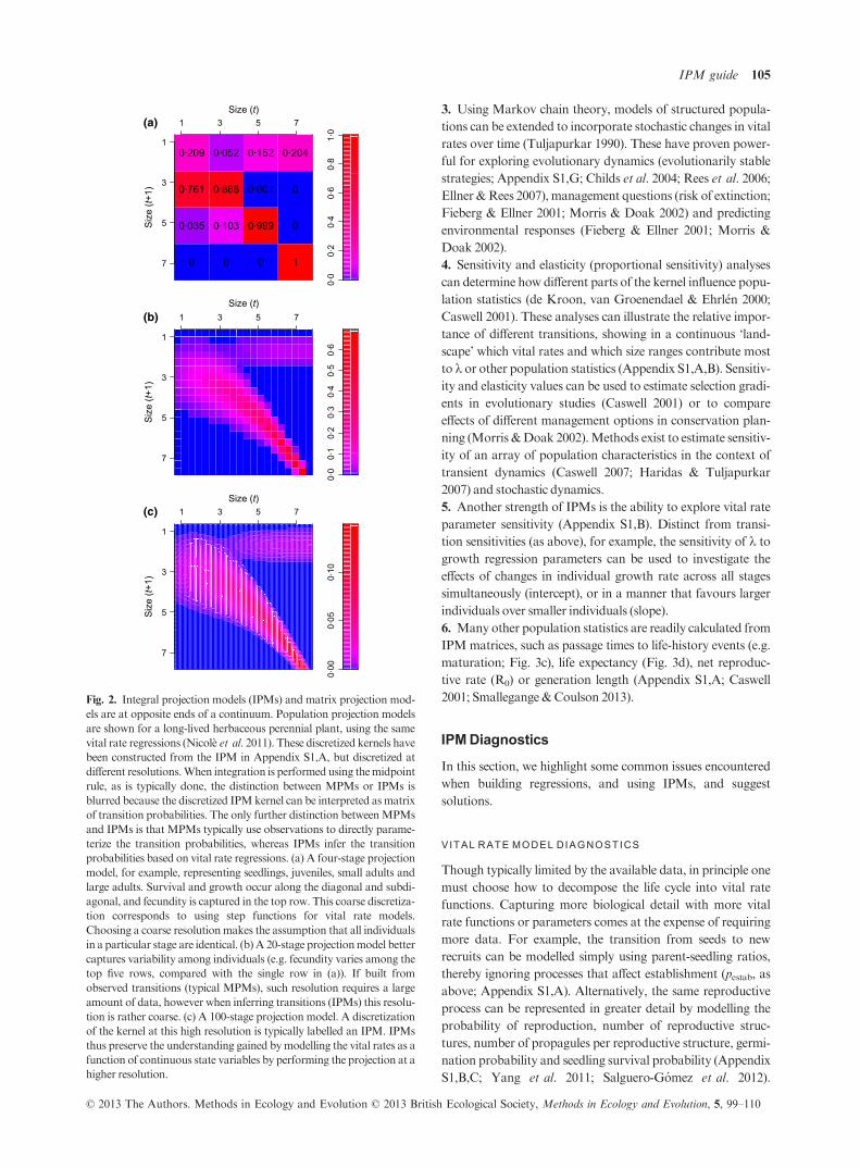
Fig. 2. Integral projection models (IPMs) and matrix projection mod-

els are at opposite ends of a continuum. Population projection models

are shown for a long-lived herbaceous perennial plant, using the same

vital rate regressions (Nicol�e et al. 2011). These discretized kernels havebeen constructed from the IPM in Appendix S1,A, but discretized at

different resolutions.When integration is performed using themidpoint

rule, as is typically done, the distinction between MPMs or IPMs is

blurred because the discretized IPMkernel can be interpreted asmatrix

of transition probabilities. The only further distinction betweenMPMs

and IPMs is that MPMs typically use observations to directly parame-

terize the transition probabilities, whereas IPMs infer the transition

probabilities based on vital rate regressions. (a) A four-stage projection

model, for example, representing seedlings, juveniles, small adults and

large adults. Survival and growth occur along the diagonal and subdi-

agonal, and fecundity is captured in the top row. This coarse discretiza-

tion corresponds to using step functions for vital rate models.

Choosing a coarse resolutionmakes the assumption that all individuals

in a particular stage are identical. (b)A 20-stage projectionmodel better

captures variability among individuals (e.g. fecundity varies among the

top five rows, compared with the single row in (a)). If built from

observed transitions (typical MPMs), such resolution requires a large

amount of data, however when inferring transitions (IPMs) this resolu-

tion is rather coarse. (c) A 100-stage projection model. A discretization

of the kernel at this high resolution is typically labelled an IPM. IPMs

thus preserve the understanding gained bymodelling the vital rates as a

function of continuous state variables by performing the projection at a

higher resolution.


IPM guide 105

Ideally, the level of biological detail is chosen based on the

importance of life-history transitions and the biological ques-

tions at hand.

The choice of state variable is also fundamentally important.

For example, size can be measured in a variety of ways, thus it

is worth exploring how vital rates vary in response to the choice

of state variable, or transforming the state variable to empha-

size certain parts of the state variable range (Appendix S1,B).

Typically, the state variable that best differentiates the size

dependence of fecundity and survival is chosen.

Even if vital rate models have a good statistical fit, they may

not be biologically reasonable for all values of the state variable

(Appendix S1,D). For example, in large-scale demographic

studies, data are typically missing for some values of the state

variable or covariates, and it is important to check whether

interpolated estimates are reasonable for unobserved cases.

For example, in Fig. 1b, we can reasonably predict growth

transitions for any individual across the range of sizes if we

believe the growth regression is satisfactory. As another exam-

ple of evaluating biological plausibility, consider survival mod-

els for long-lived canopy trees (Appendix S1,D). If mortality of

large individuals is not observed (a common issue), a standard

logistic regression can reach the asymptote of 1 andpredict that

those individuals are effectively immortal.A hierarchicalmodel

can provide a more biologically realistic survival estimate by

borrowing strength from other, better sampled groups. If col-

lecting more data at the extreme values of size is not possible,

one could set a maximum survival probability based on prior

expectations of the species’ life span. Life expectancy can be

explicitly calculated from the discretized kernel to check that

these expectations aremet (Appendix S1,A).

Accurately modelling variance is important, as this can have

a strong influence on projections. Although the expected

growth of an individual is based on the fitted model (e.g. the

regression of increment on size), the realized growth is a proba-

bility distribution around that expectation (Figs 1b and 3).

The probability distributions shown vertically in Fig. 1b illus-

trate how size at time t determines the possible sizes that an

individual might attain at time t + 1. A large variance around

the expected growth indicates that many individuals grow fas-

ter or slower than the expected amount. Because of Jensen’s

inequality, increasing the variance of growth can change the

mean population growth rate (higher or lower, depending on

the shape of the individual growth model) and lead to different

passage times and life expectancies (Fig. 3). Describing the

variation among the potential future sizes does not explain the

variation in future sizes directly, but characterizes the magni-

tude of process (and observation) uncertainty and describes

heterogeneity among individuals (cf. Clark 2003). Estimating

variance is thus biologically important (Clark 2003).

Survival/Growth Kernelwith sd = 1

Size (t)

Siz

e (t+

1)

Survival/Growth Kernelwith sd = 3

Size (t)

Siz

e (t+

1)

0 10 20 30 40 50

5

10

15

Mean life expectancy

Size

Year

s

sd = 1sd = 3

0 1 2 3 4 5 6 7

0

1

2

3

4

5

6

Passage time to size 8

Size

Year

s

sd = 1sd = 3

(a) (b)

(c) (d)

Fig. 3. A comparison of population inference due to differences in the variance in individual growth. Growth models were fit to simulated data

where the standard deviation of the fits was set at 1 and 3. This leads to (a–b) different survival/growth kernels, (c) different life expectancy patterns

and (d) different passage time patterns.


106 C. Merow et al.

It is important to consider how the predictions of the vital

rate model interact with one another to influence population

statistics. For example, if the mean growth curve described by

g(z0|z) is always greater than the 1:1 (or the z0 = z) line,

surviving individuals can grow indefinitely (Appendix S1,A). If

large individuals survive with a high probability, there is effec-

tively no upper limit on size. Conversely, the point where

g(z0|z) crosses the 1:1 line identifies the asymptotic meanmaxi-

mum size for individuals (conditional on survival). If uncon-

strained growth is unrealistic and produces extreme population

projections (i.e. unrealistically large individuals in the stable

population distribution), one should check whether the data

support alternative models that reduce growth or senescence

for large individuals (e.g. fitting a negative quadratic term in the

growth and/or survival function in Appendix S1,B,D). Alterna-

tively, parameters can be adjusted based on prior knowledge.

Vital rate regression models facilitate parsimonious and sta-

tistically grounded modelling of uncertainty in IPMs. Uncer-

tainty in regression parameter estimates can be propagated to

population statistics simply by (bootstrap) sampling from the

estimated parameter distributions and recalculating kernels

and population statistics (e.g. Ellner & Rees 2006; Jongejans,

Sheppard & Shea 2006). Regression models draw inference

across a continuous state variable, meaning that the shape of

that predictive vital rate function can be influenced by outliers,

sampling bias and other features of the model, making uncer-

tainty analyses particularly critical. Uncertainty in parameter

values may be used as a proxy for temporal variability in sto-

chastic simulation models if uncertainty likely derives from

temporal, rather than spatial, variability. Uncertainty analysis

can also be used in conjunction with sensitivity analysis to

understand the implications of uncertainty on population sta-

tistics (cf. Buckley et al. 2005; Hegland, Jongejans & Rydgren

2010). In Appendix S1,D, we discuss in more detail howmodel

structure and sample size can influence population inference.

KERNEL DIAGNOSTICS

Once the kernel is specified, it is important to evaluate whether

population statistics are affected by the choice of integration

method and size limits (Metcalf et al. 2013; Ω in eqn 1), and

whether those statistics correspond to observed (or expert

opinion) population characteristics. When discretizing the

kernel, the grid resolution should be sufficiently high to accu-

rately characterize the topography of the kernel, avoiding grid

cells that large enough to average over peaks and valleys.

When this is done, using the midpoint rule for integration

should be sufficient. However, the midpoint rule can be

impractical for slow-growing species (e.g. trees) that require

extremely large matrices (Zuidema et al. 2010). Any of a

number of numerical integration methods can be used, the

details of which are beyond the scope of this guide.

A common problem that can result from a poor choice of

size limits is the unintentional ‘eviction’ of individuals, which

leads to underestimation of survival (Appendix S1,A; Dalgle-

ish et al. 2011; Williams, Miller & Ellner 2012). Because the

growth and recruit size distributions are probability densities

than can extend to �∞, predicted values can fall outside of

the size range chosen for the IPM, causing individuals to be

‘evicted’ from the model. Detecting eviction is straightfor-

ward: the predicted values of size-specific survival (for

growth) and size-specific establishment (for reproduction)

should equal the column sums of the discretized survival/

growth and fecundity kernels, respectively. If the column

sums are lower than the predicted values, individuals will be

evicted from projections. One can resolve eviction either by

transforming the data or using non-Gaussian distributions,

so that transitions are not predicted beyond the range of the

models (Williams, Miller & Ellner 2012). Eviction can also

be resolved by expanding the size range in the model to

include sizes that were previously evicted, or adding discrete

size classes at the extremes of the size range that include all

individuals predicted at sizes beyond the extremes with an

upper/lower bound on the transition probability (Appendices

A, F; Williams, Miller & Ellner 2012).

Ecologists are likely to have substantial prior knowledge

about population statistics that are easy to obtain from any

IPM, which can help to diagnose the plausibility of a model.

For example, populations in a stable environment can be

expected to have an asymptotic growth rate close to 1 (between

0�95 and 1�05 for the forest herb modelled in Appendix S1,F).

In contrast, populations in unstable (abiotic or biotic) environ-

ments can be expected to have growth rates different from 1.

As a second example, the majority of established individuals in

stable populations of long-lived species would typically be

large. In contrast, increasing populations of short-lived species

with high adult mortality rates compensated by high rates of

recruitment should be composedmainly of smaller individuals.

As a third example, in populations with high reproductive out-

put but low juvenile survival rates, reproductive value would

be expected to increase dramatically with size, such that a large

reproductive individual of a long-lived species may have a

reproductive value that is several orders of magnitude higher

than that of a juvenile. In contrast, in a population where large

individuals have a high risk of mortality, reproductive values

would not be expected to differ much between individuals of

different size. In short, the practitioner should rely on the

fundamentals of comparative demography.

Many other model diagnostics are equivalent to those used

for MPMs; hence, the vast literature on MPM construction

also applies to IPMs (Caswell 2001;Morris &Doak 2002). For

example, the projected timing of critical life-history events such

as age at first reproduction, generation time and mean life

expectancy should match observations should be consistent

with field data or conventional knowledge (Fig. 3; Caswell

2001). Also, calculating confidence (credible) intervals on pop-

ulation statistics from bootstrap analysis (posterior samples) is

critical to determine whether the IPM reasonably narrows

down the range of possible population dynamics (Alvarez-

Buylla & Slatkin 1994). Understanding the range of possible

predictions is particularly important for IPMs because demo-

graphic transitions are interpolated from vital rate regressions

and estimates of uncertainty help quantify the quality of that

interpolation.


IPM guide 107

Biological challenges for IPMs

Integral projection models enable biologists to address old but

important questions in a new, mechanistically informed

manner. Below, we highlight some promising biological

advances made possible by IPMs and discuss their inherent

challenges to highlight avenues for future research.

Much of the theoretical development and application of

IPMs have taken place in the context of plant populations and

although extension to animal is typically straightforward,

some unique challenges may exist when modelling animal

populations. The larger number of potential state variables rel-

evant for animals, compared with plants, could necessitate

more sophisticated techniques of numerical integration, as the

commonly used midpoint rule will be inefficient for high

dimensional integrals. One area where IPMs could make an

important contribution is in the development of demographic

models structured by sex (Schindler et al. 2013), behavioural

(e.g. date of egg laying) or physiological (e.g. immune function)

measures of state. Longitudinal physiological data from field

populations are starting to become available (e.g. Nussey et al.

2011), which paves the way for data-driven models that link

physiology and population dynamics. The theory for such

models is already well worked out (Ellner & Rees 2006),

though significant practical challenges need to be overcome.

Missing data in animal populations often presents challenges,

and imputing state variables using hierarchical models may be

necessary (cf. Colchero, Jones&Rebke 2012).

Implicit and explicit spatial population dynamics can be

included in IPMs by bringing together local demography and

dispersal (Jongejans, Skarpaas & Shea 2008). One way of

incorporating spatial structure of multiple populations into a

traditional matrix model is to build a ‘mega-matrix’ model,

wherein each submatrix represents a different population and

dispersal is captured by transitions among the submatrices

(Hunter &Caswell 2005). Neighbourhood-specific competitive

interactions can also be captured with spatially implicit models

(Adler, Ellner & Levine 2010; Adler, Dalgleish & Ellner 2011).

By modelling vital rates as a function of environment (e.g. pre-

cipitation), IPMs can be used to forecast the spatial distribu-

tion of population dynamics (Appendix S1,F). Spatially

explicit IPMs also borrow from traditional matrix model

approaches: Jongejans et al. (2011) combined the IPM frame-

work with integrodifference equation models for spread in dis-

crete time and homogeneous space (Neubert & Caswell 2000).

If spatial heterogeneity is important, a simulation approach

can be used to redistribute individuals at each time step among

populations based on a dispersal kernel (Record 2010).

Integral projection models can produce proxies for fitness,

such as population growth rates given phenotype differences;

this application falls at the nexus between evolutionary biology

and ecology. At a scale that could be referred to as ‘meso-

evolutionary’ – that is, models of a single species, with implicit,

relatively simple genetics, stochastic IPMs have been used to

successfully predict the evolutionarily stable life-history strate-

gies for maturation and offspring size: projections often closely

resemble trait distributions observed in natural populations

(Appendix S1,D; Rees & Rose 2002; Metcalf, Rose & Rees

2003; Metcalf & Pavard 2007; Childs et al. 2011; Miller et al.

2012). IPMs have also been used to understand short-term

eco-evolutionary dynamics of population size distributions,

genotype distributions and other state variables in response to

environmental change (Coulson, Tuljapurkar & Childs 2010;

Coulson 2012; Smallegange & Coulson 2013). Extending the

power of these evolutionary analyses will require the incorpo-

ration of additional state variables. The introduction of

two-sex IPMs could be used to describe the complexities of

frequency dependence. More realistic representations of the

quantitative genetic structure underlying traits are another

challenging but important direction.

Density dependence may be difficult to quantify at the indi-

vidual level but models without density dependence can result

in unrealistic projections of stage structure (Appendix S1,G;

Metcalf, Rose & Rees 2003; Hesse, Rees & M€uller Scharer

2008; Dahlgren & Ehrl�en 2009; Eager et al. 2013). A recently

developed approach that can incorporate density dependence

relies on using a time-series of the population size distribution

to constrain projections (Ghosh, Gelfand & Clark 2012).

Future IPM researchwould benefit from a synthesis of popula-

tion-level data (repeated observations of state distributions) to

improve the accuracy of projections while using individual-

level data to understand how underlying vital rates relate to

state transitions (Ellner 2012).

IPMs are useful for understanding population-level patterns

that could not be inferred from data on survival, growth and

fecundity, or models of these vital rates alone. The ease of

incorporating biotic and abiotic factors into vital rate models

places demography in an ecological context. This leads to a

more mechanistic understanding of populations and poten-

tially better predictions of population dynamics – both in eco-

logical and evolutionary terms (Smallegange &Coulson 2013).

IPMs offer ecologists a powerful workflow – from data,

through vital rate models, to population inference –with every

step of IPM development requiring hypotheses, diagnostics

and ecological understanding.

Acknowledgements

This paper originated during a working group on IPMs hosted at theMax Plank

Institute for Demographic Research (MPIDR; Rostock, Germany). We thank

Florence Nicol�e for providing data forAppendices A andG. C.M. acknowledges

funding from NSF Grant 1046328 and NSF Grant 1137366. R.S.-G, C.J.E.M,

S.M, C.M. and E.J. acknowledge financial support for the working group from

the EvolutionaryDemography laboratory andModeling the Evolution ofAging-

independent group of the MPIDR. E.J. further acknowledges financial support

from the Netherlands Organization for Scientific Research (NWO-meerwaarde

Grant 840.11.001). DZC acknowledges support from the Natural Environment

ResearchCouncil (NE/I022027/1).

References

Adler, P.B., Dalgleish, H.J. & Ellner, S.P. (2011) Forecasting plant community

impacts of climate variability and change: when do competitive interactions

matter? Journal of Ecology, 100, 478–487.Adler, P.B., Ellner, S.P. & Levine, J.M. (2010) Coexistence of perennial plants: an

embarrassment of niches.Ecology Letters, 13, 1019–1029.Alvarez-Buylla, E.R. & Slatkin, M. (1994) Finding confidence limits on popula-

tion growth rates: three real examples revised.Ecology, 75, 255–260.


108 C. Merow et al.

Bruno, J., Ellner, S., Vu, I., Kim, K. &Harvell, C. (2011) Impacts of aspergillosis

on sea fan coral demography: modeling a moving target. Ecological Mono-

graphs, 81, 123–139.Buckley, Y.M., Brockerhoff, E., Langer, L., Ledgard, N., North, H. & Rees, M.

(2005) Slowing down a pine invasion despite uncertainty in demography and

dispersal. Journal of Applied Ecology, 42, 1020–1030.Caswell, H. (2001) Matrix Population Models: Construction, Analysis, and Inter-

pretation. Sinauer, Sunderland,MA.

Caswell, H. (2007) Sensitivity analysis of transient population dynamics. Ecology

Letters, 10, 1–15.Childs,D.Z., Rees,M.,Rose,K.E.,Grubb,P.J. &Ellner, S.P. (2003) Evolutionof

complex flowering strategies: an age- and size-structured integral projection

model.Proceedings of theRoyal SocietyB:Biological Sciences, 270, 1829–1838.Childs, D.Z., Rees, M., Rose, K.E., Grubb, P.J. & Ellner, S.P. (2004) Evolution

of size-dependent flowering in a variable environment: construction and analy-

sis of a stochastic integral projection model. Proceedings of the Royal Society

B: Biological Sciences, 271, 425–434.Childs, D.Z., Coulson, T.N., Pemberton, J.M., Clutton-Brock, T.H. & Rees, M.

(2011) Predicting trait values and measuring selection in complex life histories:

reproductive allocation decisions in Soay sheep.Ecology Letters, 14, 985–992.Clark, J.S. (2003) Uncertainty and variability in demography and population

growth: a hierarchical approach.Ecology, 84, 1370–1381.Colchero, F., Jones, O.R. & Rebke, M. (2012) BaSTA: an R package for Bayes-

ian estimation of age-specific survival from incomplete mark-recapture/recov-

ery datawith covariates.Methods in Ecology and Evolution, 3, 466–470.Coulson, T. (2012) Integral projections models, their construction and use in

posing hypotheses in ecology.Oikos, 121, 1337–1350.Coulson, T., Tuljapurkar, S. & Childs, D.Z. (2010) Using evolutionary demogra-

phy to link life history theory, quantitative genetics and population ecology.

Journal of Animal Ecology, 79, 1226–1240.Coulson, T., MacNulty, D.R., Stahler, D.R., vonHoldt, B., Wayne, R.K. &

Smith,D.W. (2011)Modeling effects of environmental change onwolf popula-

tiondynamics, trait evolution, and life history.Science, 334, 1275–1278.Dahlgren, J.P. &Ehrl�en, J. (2009) Linking environmental variation to population

dynamics of a forest herb. Journal of Ecology, 97, 666–674.Dahlgren, J.P. & Ehrl�en, J. (2011) Incorporating environmental change over suc-

cession in an integral projection model of population dynamics of a forest

herb.Oikos, 120, 1183–1190.Dahlgren, J., Garc�ıa, M.B. & Ehrl�en, J. (2011) Nonlinear relationships between

vital rates and state variables in demographicmodels.Ecology, 92, 1–7.Dalgleish, H.J., Koons, D.N., Hooten, M.B., Moffet, C.A. & Adler, P.B. (2011)

Climate influences the demography of three dominant sagebrush steppe plants.

Ecology, 92, 75–85.Eager, E.A., Haridas, C.V., Pilson, D., Rebarber, R. & Tenhumberg, B. (2013)

Disturbance frequency and vertical distribution of seeds affect long-termpopu-

lation dynamics: a mechanistic seed bank model. American Naturalist, 182,

180–190.Easterling, M., Ellner, S. & Dixon, P. (2000) Size-specific sensitivity: applying a

new structured populationmodel.Ecology, 81, 694–708.Ellner, S.P. (2012) Comments on: Inference for size demography from point pat-

tern data using integral projection models. Journal of Agricultural, Biological,

and Environmental Statistics, 17, 682–689.Ellner, S. & Rees, M. (2006) Integral projection models for species with complex

demography.AmericanNaturalist, 167, 410–428.Ellner, S. & Rees, M. (2007) Stochastic stable population growth in integral pro-

jection models: theory and application. Journal of Mathematical Biology, 54,

227–256.Evans,M.E.K., Holsinger, K.E. &Menges, E.S. (2010) Fire, vital rates, and pop-

ulation viability: a hierarchical Bayesian analysis of the endangered Florida

scrubmint.EcologicalMonographs, 80, 627–649.Fieberg, J. & Ellner, S.P. (2001) Stochastic matrix models for conservation and

management: a comparative review ofmethods.Ecology Letters, 4, 244–266.Ghosh, S.,Gelfand,A.E.&Clark, J.S. (2012) Inference for size demography from

point pattern data using integral projection models. Journal of Agricultural,

Biological, and Environmental Statistics, 17, 641–667.Haridas, C.V. & Tuljapurkar, S. (2007) Time, transients and elasticity. Ecology

Letters, 10, 1143–1153.Hegland, S.J., Jongejans, E. & Rydgren, K. (2010) Investigating the interaction

between ungulate grazing and resource effects on Vaccinium myrtillus popula-

tions with integral projectionmodels.Oecologia, 163, 695–706.Hesse, E., Rees, M. & M€uller Sch€arer, H. (2008) Life-history variation in con-

trasting habitats: flowering decisions in a clonal perennial herb (Veratrum

album).AmericanNaturalist, 172, E196–E213.Hunter, C.M. & Caswell, H. (2005) The use of the vec-permutation matrix in

spatial matrix populationmodels.EcologicalModelling, 188, 15–21.

Jacquemyn, H., Brys, R. & Jongejans, E. (2010) Size-dependent flowering and

costs of reproduction affect population dynamics in a tuberous perennial

woodland orchid. Journal of Ecology, 98, 1204–1215.Jongejans, E., Sheppard, A.W. & Shea, K. (2006) What controls the population

dynamics of the invasive thistle Carduus nutans in its native range? Journal of

Applied Ecology, 43, 877–886.Jongejans, E., Skarpaas, O. & Shea, K. (2008) Dispersal, demography and spatial

population models for conservation and control management. Perspective in

Plant Ecology, Evolution and Systematics, 9, 153–170.Jongejans, E., Shea, K., Skarpaas, O., Kelly, D. &Ellner, S. (2011) Importance of

individual and environmental variation for invasive species spread: a spatial

integral projectionmodel.Ecology, 92, 86–97.de Kroon, H., van Groenendael, J. & Ehrl�en, J. (2000) Elasticities: a review of

methods andmodel limitations.Ecology, 81, 607–618.Kuss, P., Rees, M., Aegisd�ottir, H.H., Ellner, S.P. & St€ocklin, J. (2008) Evolu-

tionary demography of long-lived monocarpic perennials: a time-lagged inte-

gral projectionmodel. Journal of Ecology, 96, 821–832.Metcalf, C.J.E., McMahon, S.M. & Clark, J.S. (2009a) Overcoming data sparse-

ness and parametric constraints in modeling of tree mortality: a new nonpara-

metric Bayesianmodel.Canadian Journal of Forestry Research, 39, 1677–1687.Metcalf, C.J.E. & Pavard, S. (2007) Why evolutionary biologists should be

demographers.Trends in Ecology and Evolution, 22, 205–212.Metcalf, J., Rose,K.&Rees,M. (2003) Evolutionary demography ofmonocarpic

perennials.Trends in Ecology and Evolution, 18, 471–480.Metcalf, C., Rose, K., Childs, D., Sheppard, A., Grubb, P. & Rees, M. (2008)

Evolution of flowering decisions in a stochastic, density-dependent environ-

ment.Proceedings of the National Academy of Sciences, 105, 10466.

Metcalf, C., Horvitz, C., Tuljapurkar, S. & Clark, D. (2009b) A time to grow and

a time to die: a new way to analyze the dynamics of size, light, age, and death

of tropical trees.Ecology, 90, 2766–2778.Metcalf, C., McMahon, S.M., Salguero-G�omez, R. & Jongejans, E. (2013) IPM-

pack: an R package for integral projection models. Methods in Ecology and

Evolution, 4, 195–200.Miller, T.E.X., Williams, J.L., Jongejans, E., Brys, R. & Jacquemyn, H. (2012)

Evolutionary demography of iteroparous plants: incorporating non-lethal

costs of reproduction into integral projection models. Proceedings of the Royal

Society B: Biological Sciences, 279, 2831–2840.Morris,W. &Doak, D. (2002)Quantitative Conservation Biology: the Theory and

Practice of Population Viability Analysis. Sinauer Associates, Sunderland,

MA.

Neubert, M.G. & Caswell, H. (2000) Demography and dispersal: calculation and

sensitivity analysis of invasion speed for structured populations. Ecology, 81,

1613–1628.Nicol�e, F., Dahlgren, J.P., Vivat, A., Till-Bottraud, I. & Ehrl�en, J. (2011) Interde-

pendent effects of habitat quality and climate on population growth of an

endangered plant. Journal of Ecology, 99, 1211–1218.Nussey, D.H.,Watt, K., Pilkington, J.G., Zamoyska, R&McNeilly, T.N. (2011)

Age-related variation in immunity in a wild mammal population. Aging Cell,

11, 178–180.Ozgul, A., Childs, D.Z., Oli, M.K., Armitage, K.B., Blumstein, D.T., Olson,

L.E., Tuljapurkar, S. & Coulson, T. (2010) Coupled dynamics of body mass

and population growth in response to environmental change. Nature, 466,

482–485.Ozgul,A., Coulson,T., Reynolds,A., Cameron, T.C.&Benton,T.G. (2012) Pop-

ulation responses to perturbations: the importance of trait-based analysis illus-

trated through amicrocosm experiment.AmericanNaturalist, 179, 582–594.R Core Team (2013) R: A Language and Environment for Statistical Computing.

RFoundation for Statistical Computing, Vienna, Austria.

Ramula, S., Rees,M.&Buckley,Y.M. (2009) Integral projectionmodels perform

better for small demographic data sets than matrix population models: a case

study of two perennial herbs. Journal of Applied Ecology, 46, 1048–1053.Record, S. (2010)ConservationWhile Under Invasion: Insights from a Rare Hemi-

parasitic Plant, SwampLouseword (Pedicularis lanceolataMichx.). PhDthesis,

University ofMassachusetts, Amherst,Massachusetts

Rees,M.&Ellner, S. (2009) Integral projectionmodels for populations in tempo-

rally varying environments.EcologicalMonographs, 78, 575–594.Rees, M. & Rose, K.E. (2002) Evolution of flowering strategies in Oenothera

glazioviana: an integral projection model approach. Proceedings of the Royal

Society B: Biological Sciences, 269, 1509–1515.Rees,M., Childs, D.Z.,Metcalf, J.C., Rose, K.E., Sheppard, A.W. &Grubb, P.J.

(2006) Seed dormancy and delayed flowering in monocarpic plants: selective

interactions in a stochastic environment.AmericanNaturalist, 168, E53–E71.Salguero G�omez, R. & Plotkin, J.B. (2010) Matrix dimensions bias demographic

inferences: implications for comparative plant demography. American Natu-

ralist, 176, 710–722.


IPM guide 109

Salguero-G�omez, R., Siewert, W., Casper, B.B. & Tielborger, K. (2012) A

demographic approach to study effects of climate change in desert plants.

Philosophical Transactions of the Royal Society B: Biological Sciences, 367,

3100–3114.Schindler, S., Neuhaus, P., Gaillard, J.-M. & Coulson, T. (2013) The influ-

ence of nonrandom mating on population growth. American Naturalist,

182, 28–41.Smallegange, I.M. & Coulson, T. (2013) Towards a general, population-level

understanding of eco-evolutionary change. Trends in Ecology and Evolution,

28, 143–148.Tuljapurkar, S. (1990) Population Dynamics in Variable Environments. Lecture

Notes in Biomathematics 85, Springer, NewYork.

Wallace,K., Leslie, A.&Coulson, T. (2012)Re-evaluating the effect of harvesting

regimes on Nile crocodiles using an integral projection model. Journal of

Animal Ecology, 82, 155–165.Williams, J.L., Miller, T.E. & Ellner, S.P. (2012) Avoiding unintentional eviction

from integral projectionmodels.Ecology, 93, 2008–2014.Yang, S., Jongejans, E., Yang, S. & Bishop, J.G. (2011) The effect of consumers

andmutualists ofVacciniummembranaceum atMount St. Helens: dependence

on successional context.PLoSONE, 6, e26094.

Yule,K.M.,Miller, T.E.X.&Rudgers, J.A. (2013)Costs, benefits, and loss of ver-

tically transmitted symbionts affect host population dynamics. Oikos, 122,

1512–1520.Zuidema, P.A., Jongejans, E., Chien, P.D., During, H.J. & Schieving, F. (2010)

Integral Projection Models for trees: a new parameterization method and a

validation ofmodel output. Journal of Ecology, 98, 345–355.

Received 23 September 2013; accepted 19November 2013

Handling Editor: Satu Ramula

Supporting Information

Additional Supporting Information may be found in the online version

of this article. Data for examples in supplementary materials is available

at DOI: 10.5061/dryad.6575f

Appendix S1.Rcode for various IPMs.


110 C. Merow et al.

advancing population ecology with integral projection...

Documents