NASA Contractor Report 4753

Aeroelastic Calculations Using CFD for aTypical Business Jet Model

Michael Do Gibbons

Contract NAS1-19000

Prepared for Langley Research Center

September 1996

https://ntrs.nasa.gov/search.jsp?R=19970001894 2018-05-19T14:08:37+00:00Z

NASA Contractor Report 4753

Aeroelastic Calculations Using CFD for aTypical Business Jet Model

Michael D. Gibbons

Lockheed Martin Engineering & Sciences Company • Hampton, Virginia

National Aeronautics and Space AdministrationLangley Research Center ° Hampton, Virginia 23681-0001

Prepared for Langley Research Centerunder Contract NAS1-19000

September 1996

Printed copies available from the following:

NASA Center for AeroSpace Information

800 Elkridge Landing Road

Linthicum Heights, MD 21090-2934

(301) 621-0390

National Technical Information Service (NTIS)5285 Pon Royal Road

Springfield, VA 22161-2171

(703) 487-4650

Aeroelastic Calculations Using CFD for a Typical BusinessJet Model

In MemoriamMichael D. Gibbons

(1960 -- 1994)

This report is being published posthumously and is dedicated to the author,

Michael D. Gibbons. It should be noted that this report was not complete at

the time of Mike's death. He had mentioned to several of his co-workers that

he had gathered all of the information necessary to complete the report, but

obviously had not had time to process and incorporate all of the data. Mike

was a meticulous note-taker, and so with very little effort, we were able to find

and extract the necessary information to complete and publish this valuable, well-

presented, research. This report stands as a testament to the accuracy, attention

to detail, and overall thoroughness Mike applied to all facets of his work.

In the fall of 1994, Mike's Lockheed and NASA co-workers had resigned

themselves to the fact that their day-to-day relationship with him was about

to change drastically, since he had recently accepted a position with Boeing in

Seattle, Washington. Nobody truly felt Mike was leaving since he would always

be a phone call, or as he preferred, an e-mail message away. Everyone was

excited for him and preparing to offer their best-wishes and farewells when he

tragically died just two days before his scheduled departure.

Mike dedicated virtually his entire career to aeroelastic analysis and the

prediction of flutter. He was responsible for the development and verification

of many of the flutter prediction techniques using computational fluid dynamics

in practice today. His work in the application of Transonic Small Disturbance

(TSD) potential flow methods to problems in aeroelasticity is unsurpassed. Due

to this work, he had established himself as one of the premier computational

aeroelasticians in the industry. The research discussed in this report breaks ground

in several different areas. From a numerical standpoint, it is a comprehensive

study of the impact of varying equation accuracy on unsteady aerodynamic and

aeroelastic simulations. Data are presented and compared using methods ranging

from linear theory to TSD to full Euler/Navier-Stokes formulations. Second, and

more importantly, it provides valuable insight into the role of viscous effects in

flutter, especially in the vicinity of the "transonic dip."

This effort was basically Mike's first foray into the world of Euler/Navier-

Stokes aerodynamics and its application to aeroelastic problems. As evidenced by

this report, it is obvious that he possessed the talent, willingness and dedication

required to excel in this field, and the industry will miss him dearly.

To many of us, Mike was a loyal friend who cheered us with his kindness

and warm smile. He touched us deeply, and along with his family, we grieve

his untimely death. We will always have those happy memories of working and

playing with this special friend. His passing has left not only a technical void in

the Langley community, but an emotional one as well.

Aeroelastic Calculations Using CFD

for a Typical Business Jet Model

Michael D. Gibbons

Lockheed Martin Engineering and Sciences Company

Summary

Two time-accurate Computational Fluid Dynamics (CFD) codes were used

to compute several flutter points of a typical business jet wind tunnel model.

The model consisted of a rigid fuselage with a flexible semispan wing and was

tested in the Transonic Dynamics Tunnel at NASA Langley Research Center

where experimental flutter data were obtained from Mo_----0.628 to Moo---0.888.

The computational results were computed using CFD codes based on the inviscid

TSD equation (CAP-TSD) and the Euler/Navier-Stokes equations (CFL3D-AE).

Comparisons are made between analytical results and with experiment where

appropriate. The results presented here show that the Navier-Stokes method is

required near the transonic dip due to the strong viscous effects while the TSD

and Euler methods used here provide good results at the lower Mach numbers.

Nomenclature

C

Cr

ct

C

ct

Cp

f, Hz.

fiK

m

M

Moo

qi

q_

O

S

local chord

root chord (1.8942 ft)

tip chord (0.5433 ft)

damping matrix

sectional lift coefficient

pressure coefficient

frequency

mode shapes (i=l, 6)

stiffness matrix

mass of wing (0.56522 Slugs)

mass matrix

freestream Mach number

generalized displacements (i=l, 6)

freestream dynamic pressure

generalized forces

semi-span of wing (4.0392 ft)

t

UfV

Vf

x,y,z

#

Pf

_f

nondimensional time

flutter velocity

volume of truncated cone that encloses wing (5.1945 ft 3)

flutter speed index 2u

nondimensional cartesian coordinates

ratio of specific heats

mass ratio

flutter density

small disturbance potential

flutter frequency, rad./sec.

modal frequencies (i=l, 6), rad./sec.

Introduction

Several years ago a significant effort was devoted to the development of a

Computational Fluid Dynamics (CFD) method that solves the inviscid Transonic

Small Disturbance (TSD) equation for use in aeroelastic analysis. This work was

undertaken in order to provide an alternative to the widely used linear methods,

such as doublet lattice, and to improve upon previous TSD codes. The code

developed to solve the TSD equation is called CAP-TSD tl' 21 and allows transonic

effects to be included in flutter calculations. Subsequent to the CAP-TSD effort,

a version of CFL3D [3' 4] which solves the Euler/Navier-Stokes equations was

modified to allow dynamic aeroelastic calculations, tS] This version of the code is

known as CFL3D-AE, and it was used to compute all of the Euler/Navier-Stokes

calculations presented in this report. The advantage of using the Euler/Navier-

Stokes equations is the improved accuracy in modeling the flow physics. Both

CAP-TSD and CFL3D were developed at NASA Langley Research Center.

The purpose of this report is to further assess the above CFD methods for

transonic flutter applications. Previously CAP-TSD has been used to compute the

flutter boundary of various wings, including thin highly swept delta wings, t6, 7]

the AGARD 445.6 wing, [8] and an Active Flexible Wing. [9] CFL3D has been used

to solve the Euler [l°l and the Navier-Stokes I11l equations for the AGARD 445.6

wing. This report presents results for a typical business jet configuration [12l that

was tested in the Transonic Dynamics Tunnel at NASA Langley Research Center.

The results include spatial and temporal convergence studies, surface pressure

coefficient comparisons for rigid and statically deformed cases, and a discussion

of the aeroelastic results using the TSD, Euler, and Navier-Stokes methods.

Numerical Method

This section gives a brief description of the methods used to numerically

solve the TSD, Euler/Navier-Stokes, and aeroelastic equations as contained in the

CAP-TSD and CFL3D computer codes, respectively.

The CAP-TSD code solves the unsteady transonic small disturbance equa-

tion using an implicit time-accurate approximate factorization algorithm with the

optional use of internal subiterations to minimize linearization and factorization

errors. The unsteady aerodynamics are simultaneously integrated in time along

with the structural equations of motion, which allows a time history of the struc-

tural response to some initial conditions to be studied. The structure is modeled as

a series of orthogonal mode shapes weighted by time varying coefficients known

as the generalized displacements. Since the modal deflections in the streamwise

and spanwise directions are small in comparison to the vertical modal displace-

ments, they are neglected and the position of the wing at any point in time can

be given by

modes

z(x,y,t)= E qi(t)fi(x,y)i

where qi is the time varying generalized displacements and fi represents the

vertical components of the mode shapes. This allows the structural equations

of motion to be written in generalized coordinates

[M]{_} + [C]{/t} + [K]{q} = {Q}

where [M], [C], and [K] are the generalized mass, damping and stiffness matrices

and {Q} is the generalized aerodynamic forces. The unsteady aerodynamics

can be computed using different forms of the TSD equation by choosing different

coefficients. Two different forms of the TSD equation were used here by choosing

either the linear equation coefficients or the so-called AMES coefficients. The

linear results were computed using the form

a 2ML )-_ (-M_ ck, -

0

+ _(0 -/L)_)

0

+

)=o

The nonlinear results were computed using the TSD equation written using the

AMES coefficients given by

0. M2 2M_¢,)N(- -

+ _x (i - ML)¢, - 7(7 + 1)M2¢_ + 7(3' -

0

+ _y (¢, (1 - (')' - 1)MLCz))

=0

When the linear equation was used, the wing was modeled as a flat plate in order

to produce results similar to other linear methods such as doublet lattice. When the

nonlinear equation was used, the wing was modeled using the appropriate airfoil

shapes so that nonlinear effects (such as moving shock waves) could be modeled.

All CAP-TSD calculations included the effects of shock generated entropy and

vorticity. 113] The linear pressure coefficient equation was used to compute the

surface pressure values. Version 1.3 of CAP-TSD was used in all calculations.

The CFL3D code solves either the Euler or Navier-Stokes equations using an

implicit time-accurate approximate factorization algorithm involving either flux

vector splitting or flux difference splitting. For the calculations presented here,

flux-vector splitting was used. For the Navier-Stokes calculations, turbulence was

modeled using the Baldwin-Lomax model. Coupling of the structural equations of

motion with the aerodynamics was done similar to that implemented in CAP-TSD.

As with CAP-TSD, only the vertical component of the mode shape is used.

Aeroelastic Calculations for a Typical Business Jet

This section discusses the numerical results obtained for a business jet con-

figuration. Details of the geometry and the CFD models used in the calculations

are included. Every attempt was made to verify the spatial and temporal con-

vergence of the solutions. Results are presented which show the convergence of

selected cases. Sensitivity of the aeroelastic solutions to the initial conditions are

also presented. Surface pressure comparisons are made for the static rigid and

static aeroelastic cases. Finally, dynamic aeroelastic results are presented using

different equation levels, and comparisons are made with experimental data.

Model Geometry

The business jet configuration consisted of a semispan wing/fuselage con-

figuration which was tested in the Transonic Dynamics Tunnel (TDT) at NASA

Langley Research Center. Figure 1 shows an illustration of this model mounted on

the wall of the TDT. The model was tested in air for a range of freestream Mach

numbersto obtain flutter points. The model, however, was not instrumented to

measure surface pressure data. Experimental flutter data were obtained for Mach

numbers ranging from 0.628 to 0.888 [141. The wing root angle-of-attack was var-

ied during the test to minimize loading with the maximum angle needed for this

purpose being 0.2 degrees. The wing has a taper ratio of 0.29 and a midchord

sweep of 23 degrees. The airfoil thickness varies from 13 percent at the symmetry

plane (for the extended wing configuration) to 8.5 percent at the wing tip. The

fuselage has a circular cross-section with a conical aft end.

The CAP-TSD calculations for the wing/fuselage configuration involved a

100x50x80 point computational grid with 45 points along the chord of the

wing and 25 points along the span. Figure 2 shows a perspective view of the

wing/fuselage surface grid. Figure 3 shows the four airfoil sections used to define

the wing surface. Linear interpolation is used to define the airfoil sections at

other spanwise locations. Calculations were also performed for a wing alone

configuration to study the effect of the fuselage on the results. Calculations for

the wing alone used the same grid as the wing/fuselage configuration but with the

wing extended to the symmetry plane.

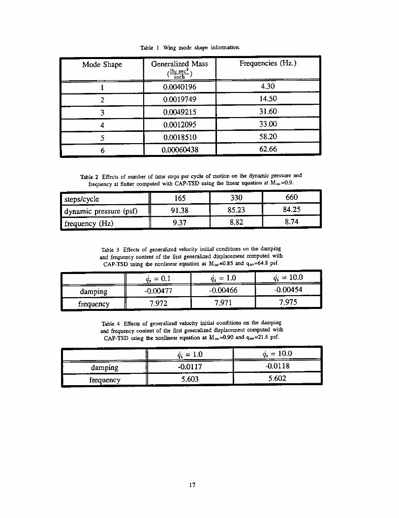
Figure 4 shows the mode shapes for the wing, and Table 1 gives the general-

ized masses and frequencies used in the aeroelastic calculations. The mode shapes

and generalized masses were computed from a finite element structural model us-

ing NASTRAN. The frequencies are experimental values measured during testing

of the model in the TDT. As with most models of this type, a yaw mode is present

which includes very small vertical displacements. In all subsequent analyses, this

yaw mode is neglected and is not shown in the above figure.

The CFL3D calculations for the extended wing were made primarily with two

grids as shown in Figures 5 and 6. The Euler mesh contained 153 points around

the airfoil and wake, 57 points out the span with some clustering around the wing

tip, and 33 points normal to the wing surface. There were 113 points around each

airfoil section and 41 points On the wing spanwise. The Navier-Stokes mesh was

virtually identical except there were 51 points normal to the wing. Both meshes

used a C-H topology. No attempt was made to model the fuselage since inviscid

TSD results showed that it has little effect on the flutter solution as discussed

later. Viscous interactions between the wing and fuselage could impact flutter

results, but detailed analyses of these types of interactions are beyond the scope

of this effort.

Spatial and Temporal Convergence

Prior to making numerous aeroelastic calculations, a convergence study was

done with CAP-TSD and the CFL3D-Euler results. The effect of time step

on the CAP-TSD solutions is shown using the linear and nonlinear equations,

and the effect of grid density is shown for a case using the nonlinear equation.

Spatial and temporal convergence of the CFL3D-Euler results are shown. No

convergence study was done using the CFL3D-Navier-Stokes version due to the

large computational time required. By making these calculations, a grid density

and time step were chosen which produced solutions of acceptable accuracy and

yet require the minimum amount of computer time.

CAP-TSD

The temporal convergence study was performed at Moo--0.6 with CAP-TSD

using the nonlinear equation and at Moo=0.9 using the linear and nonlinear

equation. Table 2 shows the effect of time step on the predicted flutter dynamic

pressure at Moo---0.9 using the linear TSD equation. The table shows the flutter

dynamic pressure and frequency computed using a time step based on 165, 330,

and 660 steps per cycle of motion in the third modal frequency (31.6 Hz).

Increasing the number of time steps from 165 to 330 results in roughly a 7

percent reduction in predicted flutter dynamic pressure whereas increasing from

330 to 660 only produces about a 1 percent reduction in flutter dynamic pressure.

Figure 7 shows the first generalized displacement computed at Moo--0.6 using

the exact same input files except for the time step. The figure shows the large

error when the solution is not converged temporally. Using a time step of 0.1

results in an unstable structural response whereas a value of 0.0339 produces a

stable structural response. Reducing the time step further to 0.0166 resulted in no

significant change from the response at 0.0339. The nonlinear case at Moo=0.9

is shown in Figure 8. The transients shown correspond to 330 and 660 steps

per cycle of motion. Figure 8 indicates that at Moo---0.9 a temporally converged

solution was obtained when using 330 steps/cycle. The time step used in the

remaining unsteady calculations was based on 330 steps per cycle of motion

since the increased accuracy at 660 was deemed minimal.

A spatial convergence study for a nonlinear case at M_--0.9 and qoo=21.6

psf is shown in Figure 9 using two different grid densities. The first grid size

was 100x50x80 and is used in all the other results computed in this paper; the

second grid size was 140x70x90. The second grid has 60 points along the chord

and 35 points along the span with clustering near the wing tip. Figure 9 shows

that the two solutions are nearly identical. This good comparison suggests that

the 100x50x80 grid produces solutions of acceptable spatial accuracy.

CFL3D-Euler

Three different grid densities were used to study spatial convergence of the

CFL3D-Euler solution at Moo--0.9 and zero degrees angle of attack. The grids

used were constructed using a C-H topology. These grids contained 153x43x33,

153x57x33, and 263x57x33 grid points. The index refers to the number of points

around the airfoil chord, spanwise, and normal to the surface, respectively. Figure

10 shows the comparisons between the three solutions. Each grid gives nearly

the same solution with the spanwise index having the greatest influence on the

location of the uppersurfaceshocknearthe wing tip, and thechordwiseindexaffecting the resolutionof a small lower surfaceshocknear the tip. Basedonthesecalculations,the 153x57x33grid wasselectedasproducinga solutionwithanacceptablelevel of spatialaccuracyfor the aeroelasticcalculationspresentedin this report.

The CFL3D-Eulercalculationsuseda time stepof 0.05 for all the unsteadyresultspresented.To determinehow sensitivethe solutionswereto time step, acalculationwasdonewith a time stepof 0.01for anaeroelasticcaseat Moo=0.9and qoo=36.0psf. Figure 11showsa plot of the first generalizeddisplacementfor thetwo different time steps.Sincethetwo solutionsarenearly identical, thelarger time stepof 0.05wasusedfor further dynamicaeroelasticcalculations.

Initial Conditions

Each dynamic aeroelastic calculation is computed by using the converged

static aeroelastic solution with some form of initial condition prescribed for the

generalized displacements or velocities of each structural mode. Typically, the

initial condition on the generalized displacements of each mode is taken to be

zero which should help to reduce numerical transients which otherwise might be

created by the wing instantaneously being displaced. To initiate the motion of

the wing, the generalized velocities of each mode have been set to 1.0 in all

the dynamic aeroelastic calculations presented unless noted otherwise. By setting

all of the generalized velocities to 1.0 (ie, cii = 1.0, i = 1,6), each mode actively

participates in the structural response. This allows for accurate values of damping

and frequency to be extracted from each generalized displacement.

The choice of using an initial generalized velocity of 1.0 is somewhat arbitrary

and its effect on the structural response depends on how the mode shapes were

scaled. To show the effect that different values have on the solution, values

of 0.1, 1.0, and 10.0 were used as initial conditions at Moo=0.85, q_=64.8

psf for the wing/fuselage configuration. These calculations were done using the

CAP-TSD code. Figure 12 shows the structural response of the first generalized

displacement. Each response was normalized by the initial condition amplitude

for direct comparison. Figure 12 indicates that the responses are quite similar,

and when damping and frequency information is extracted from each curve, the

frequency values are nearly identical, as shown in Table 3, while the damping

values range within five percent of each other. The amplitude of motion at the

wing tip leading edge caused by the different initial conditions varied from a

maximum of +/- 0.015 degrees to +/- 1.5 degrees for the initial conditions 0.1

and 10.0, respectively. These calculations indicate the aeroelastic response to

a set of initial conditions behaves in a linear fashion with the initial conditions

even though the mean flow field contains nonlinear features. Similar results were

obtained at a higher Mach number, Moo--0.9, for the wing alone case as shown

in Figure 13 and Table 4.

Methodology to Locate Flutter Crossing

To compute the point at which flutter occurs for a given Mach number, several

executions of a code are required. First, a static aeroelastic solution is computed

using a value of the dynamic pressure that is assumed to be near that which pro-

duces flutter (neutral stability). Next, a dynamic aeroelastic solution is computed

by restarting the calculation from the converged static aeroelastic solution with

some initial condition on the vertical velocity of the wing. The generalized dis-

placements from the dynamic case are fit with a series of exponentially damped

sine waves [15] allowing the stability of the system to be determined. If the aeroe-

lastic solution was stable, a higher value for the dynamic pressure is chosen and

the static and dynamic aeroelastic solutions are again computed. Once two or

more transients have been computed, the flutter dynamic pressure value is deter-

mined by linear extrapolation using the damping information from the curve fitting

process. Linear extrapolation or interpolation gives an estimate of the conditions

that produce flutter. However, further refinement can be obtained by additional

aeroelastic calculations if improved accuracy is desired.

An alternative method to calculate the flutter crossing is to vary free stream ve-

locity while holding density constant (usually to the experimental flutter density).

This approach allows the mass ratio of the calculation to match the experimental

value. Since this method generally requires that the flutter solution be known be-

fore it is computed, the method of varying density is generally used. An additional

reason to vary density rather than velocity is that the flutter dynamic pressure is

generally more sensitive to changes in density than velocity thus making it easier

to determine the point of neutral stability.

Static Rigid Results

In this section, comparisons of the surface pressure coefficients computed

with CAP-TSD and CFL3D are shown for the extended wing at zero degrees

angle of attack. Due to the lack of experimentally measured surface pressures,

comparisons are made between different codes. The most direct comparison to

make with CAP-TSD is the CFL3D-Euler results since both methods assume the

flow to be inviscid. Comparisons between CFL3D-Euler and CFL3D-Navier-

Stokes generated surface pressure distributions are shown to indicate the effect

that viscosity has on the steady solution. These calculations were made for the

extended wing configuration only since the fuselage was not modeled in the

CFL3D calculations.

Comparisons between CAP-TSD and CFL3D-Euler surface pressure coeffi-

cients are shown for Moo--0.7 and Moo=0.9 at zero degrees angle of attack. Figures

14 and 15 show that CAP-TSD compares favorably with the CFL3D-Euler re-

sults. At M_--0.7, both methods are in excellent agreement for this subsonic case.

When the Mach number is increased to 0.9, a shock wave develops along the up-

per surface with a weaker shock wave on the lower surface. Comparisons between

the two methods indicate a slight difference in the surface pressure magnitude at

some span stations. On the lower surface near midspan, CAP-TSD predicts the

shock is located further upstream than the Euler results. Part of this difference

may be due to the CAP-TSD grid which had a finer spacing in the spanwise direc-

tion near the wing root than the Euler grid did. Although not shown, additional

CAP-TSD calculations with a finer spacing at the wing trailing edge, resulted in

excellent comparisons of the surface pressure coefficients near the wing trailing

edge but the refinement had little effect on the overall surface pressures.

Comparisons are also shown between the sectional lift coefficients for the

above two cases in Figure 16. As expected, the comparison between CAP-TSD

and CFL3D is fairly good at Moo--0.7 but shows some significant differences at

Moo=0.9. These differences are due to the slight disagreement in the surface

pressures shown in Figure 15.

To show the effect that viscosity has on the position and strength of the shock

waves, a comparison was made between the CFL3D-Euler and CFL3D-Navier-

Stokes results at Moo---0.9, zero degrees angle of attack, and Re = 1.107x106. This

Reynolds number is typical of the value obtained during flutter tests this model

in the TDT. Figure 17 shows how the shock on the upper surface is significantly

weakened and shifted forward. The rapid recompression at the trailing edge is

also weakened due to the presence of the boundary layer. Aeroelastically, the

most important features are the forward shift in the shock resulting in a forward

shift in the aerodynamic center and the lower loads experienced on the wing due

to the weakening of the shock.

Static Aeroelastic Results

Prior to making a dynamic aeroelastic calculation, the wing was allowed to

deform due to the static air loads. To obtain a converged static aeroelastic solution,

six normal modes were used. A structural damping value of 0.99 (nearly critically

damped) was used for each mode while the solution was marched in time. Surface

pressure distributions are shown, and comparisons are made between CAP-TSD

and CFL3D-Euler results. The aerodynamic center and its relationship to the first

torsion node line, based on CAP-TSD calculations, are also plotted.

Figure 18 shows a three dimensional view of the upper and lower surface

pressure coefficients computed with CAP-TSD for the wing/fuselage configura-

tion. Results are shown at Moo--0.8, 0.85, 0.9, and 0.95 for the converged static

aeroelastic deflections near the flutter dynamic pressure. These figures show the

development of strong shocks on the surface of the wing. At Moo---0.95, the upper

and lower surface shock has reached the trailing edge with the recompression oc-

curring slightly downstream of the wing trailing edge. The occurrence of a shock

near the wing root trailing edge is due to the aft shape of the fuselage which

results in a rapid expansion followed by a shock. As Figure 2 shows, the fuselage

becomes conical at approximately eight tenths root chord. Figure 18 shows that

the shockcompletelydisappearswhen the aft end of the fuselagewas replacedby a cylinderextendingto thedownstreamboundary.In reality, thedevelopmentof suchstrongshocksmay not occurdue to the effect of viscosity which tendsto weakenshocksandmove them forward.

Comparisonsbetweenthe CAP-TSDand CFL3D-Eulerstaticaeroelasticso-lutions at Moo--0.7and Moo--0.9areshownin Figures 19and 20. At Moo=0.7andqoo=115.2psf, comparisonsbetweentheCAP-TSDandCFL3D-Eulerresultsare quite good. At this Mach numbera strong suction peak exists along thelower surfaceleadingedge.This is due to thenegativeeffective angleof attackproducedby the twist of the deformedwing.

At Moo=0.9and qoo=36.0psf, comparisonsbetweenCAP-TSDandCFL3D-Euler pressures(Figure 20) are good. However, CAP-TSD predicts the lowersurfaceshockwaveto be locatedfurtherforward nearthewing tip thanpredictedby CFL3D. Partof thedifferencein thesolutionsis dueto thestaticallydeformedshape. The loading predictedwith CAP-TSD results in the wing tip leadingedgebeing deflected1.81degreesnosedown whereasCFL3D-Euler predictsadeflectionof 1.74degrees.Sincetheloadson thewing wereslightly different forthe rigid case,the resultingstatic aeroelasticshapemust bedifferent.

A comparisonof thesectionallift at Moo---0.7andMoo=0.9is shownin Figure21. At Moo----0.7,the comparisonbetweenCAP-TSD andCFL3D sectionallift isfairly goodwith somediscrepancynearthe wing tip. At thehigherMachnumberof Moo--0.9,CAP-TSD tendsto predicta higher loadingat the wing tip and alower loading at wing root againdue in part to the differencein the staticallydeformedshape.

Figure 22showshow theaerodynamiccenter,computedwith CAP-TSDneartheflutter dynamicpressure,variesasthe Mach numberincreasesfrom Moo---0.7to Moo---0.9.At Moo---0.7,the aerodynamiccenteris locatedwell forward of thefirst torsion nodeline nearthequarterchordline asexpected.This is onereasonwhy subsonicallya higher dynamicpressureis requiredto produceflutter. Asthe Mach numberincreases,the aerodynamiccentermovesaft and at Moo=0.9lies close to the first torsion nodeline. This reducesthe aerodynamicdampingof the wing. With lessdampingthe dynamicpressurewhich will produceflutteris expectedto decrease.Although not shown, calculationswherethe dynamicpressurewas varied at a constantMach number indicatedlittle changein thelocation of the aerodynamiccenter.

Dynamic Aeroelastic Results

The flow conditions which produce flutter that are presented in this section

were computed using TSD, Euler and the Navier-Stokes equations. Calculations

for the wing/fuselage configuration and the extended wing configuration were

made with CAP-TSD. Since the presence of the fuselage appeared to have little

effect on the aeroelastic solutions, the Euler and Navier-Stokes calculations were

lO

madeonly for the extendedwing. Calculationsarepresentedto showthe effectof the fuselage,massratio, and equationlevel.

For eachcalculationthe resultswere tabulatedandplotted. To eliminateanypossibleconfusiononhowcertainquantitieswerecalculated,theexpressionsusedare givenhere. The massratio wascomputedusing

m

where

#- Vpf

1

V = _s(c _, + c, cr + C_r)

and 'm' is the mass of the wing, 's' is the semispan of the wing, 'ct' is the tip

chord, and 'Cr' is the root chord at the wing fuselage intersection. The subscript on

density refers to the value at flutter. The reduced frequency was computed using

k- crwt2Uf

where wf is the flutter oscillatory frequency, and Uf is the flutter free stream

speed. The flutter speed index was computed using

2UfVf-

CrY3

where w3 is the third modal frequency corresponding to first torsion.

CAP-TSD results

Several flutter points were computed with CAP-TSD using the linear and

nonlinear equations. For both sets of results, the flutter points were computed by

holding velocity constant and varying density unless stated otherwise. No struc-

tural damping was used in these calculations. All calculations were performed

with the wing root set at zero degrees angle of attack. Each dynamic aeroelastic

calculation was restarted from a converged static aeroelastic solution. The ma-

jority of the unsteady calculations were computed using 330 steps per cycle of

the third modal frequency. Typical CPU execution times were 3.1 micro seconds

per grid point per time step on a CRAY 2. Flutter data for the business jet wing

are tabulated in Tables 5 through 13. Experimental data obtained in the NASA

Langley Research Center Transonic Dynamics Tunnel are presented in Table 5

for comparison with the following computed results.

Figure 23 (Table 6) shows that the CAP-TSD linear results for the

wing/fuselage configuration at low Mach number are in excellent agreement with

the experimental results. The good agreement between CAP-TSD linear results

and experiment at the lower Mach numbers should be expected since nonlin-

ear aerodynamic effects are insignificant whereas linear theory is thought to give

reasonable answers at higher Mach numbers due to the counteracting effects of

11

thickness and viscosity. Thickness has a destabilizing effect at transonic speeds

for inviscid flows whereas viscosity tends to be stabilizing. A comparison between

the CAP-TSD results computed with the linear (Table 6) and nonlinear (Table 7)

equation in Figure 23 show that thickness has a significant effect above Moo---0.7.

The large differences between the results using the linear and nonlinear equations

are due to the presence of strong shocks in the flow field.

For the results computed with the nonlinear equation, calculations at Moo=0.9

indicated a very low dynamic pressure may have been needed to obtain a flutter

crossing. At this Mach number all solutions computed by varying density down

to a dynamic pressure of 7.2 psf were unstable with low damping. Since such

an unrealistically low dynamic pressure may have been needed to obtain a flutter

crossing no point was plotted for this case.

The effect of the fuselage on the flutter results is shown by two calculations

in which the fuselage was removed and the wing extended to the symmetry plane.

Results of this analysis are tabulated in Table 8. As shown in Figure 24, the effect

of the fuselage is minimal. This is expected since the generalized aerodynamic

forces are weighted by the mode shapes, and near the root where the interference

effects of the fuselage are greatest, the modal displacements are nearly zero thus

resulting in a contribution to the generalized aerodynamic forces which is far

smaller than the contributions from the loading near the wing tip where the modal

displacements are greatest.

Figure 25 (Table 9) shows the effect of matching the mass ratio to the

experimental value. These calculations are done by holding density constant

at a linear extrapolation of the experimental density and varying both dynamic

pressure and velocity. At Moo--0.8, there is no significant difference between

the calculations which match velocity or density. However, at Moo--0.9, a solid

flutter point was obtained with CAP-TSD while the velocity was being varied.

This is in contrast to the unstable solutions computed by varying density while

holding velocity constant. Based on the improved solutions computed by varying

velocity, one should not conclude that this provides more accurate answers than

varying density. Varying velocity effectively changes the phase lag, which has

been pointed out by Zwann [16] as being a primary cause of the transonic dip. Thus,

if the theoretical flutter velocity is significantly different from the experimental

velocity, the flow physics may not be the same as those in the experimental data

making direct comparisons meaningless. This implies the velocity should be held

fixed at the experimental value; however, a somewhat different argument might

be made for varying density which affects wing loading.

Figure 26 provides further insight into the inviscid flutter by showing the

modal interactions for the previous CAP-TSD results computed with the nonlinear

equation for the wing/fuselage configuration in root locus form. These figures

show frequency versus damping for each mode with stable roots on the left and

unstable roots on the right of each of the figures. In Figures 26a, 26b, and 26c, the

mode which first becomes unstable is first bending. These results are very similar

12

to thoseobtainedby Mohr, Batina,andYangt171who showa studyof the fluttermechanismfor awing similar to theonestudiedhere. In Reference[17]however,themassratio washeldconstant,whereasin thepresentstudy,themassratio wasallowedto vary with increasingMach number. Calculationswith CAP-TSD atlower massratiosfor the Moo=0.9case(Table 10)showedthat asthemassratiodecreases,thedynamicpressurewhich producesflutter increases,andthe typeofmodeshift shownin Reference[17] occurs;thatis, thefirst torsionmodeappearsto be theprimaryflutter mechanism.With thehighermassratiosencounteredforthe CAP-TSD calculationsvarying density,there doesnot appearto be a shiftin the primary flutter mechanism,which remainsfirst bendinginto supersonicflow. Reference[17] attributesthemodeshift to the uppersurfaceshockpassingacrossthe first torsion node line. Similar results shown here indicate that asthe shockmovesaft, there is a reductionin aerodynamicdamping due to theaft movementof the aerodynamiccenter. As the Mach numberincreasesfromMoo--0.7to Moo--0.85,the largeststablevalue of dampinggraduallydecreaseswith the frequencydecreasingfor zerodamping. The decreasein frequencyisalso shownin Figure 23b. Furthercalculationshave shownthat the third modeeventuallygoesunstable,but atmuchhigherdynamicpressures.At M_--0.9, boththe first bendingmodeandfirst torsiongounstableandappearto beunstableevenat dynamicpressuresnearzero (largemassratios).

CFL3D results

The following section presents aeroelastic results which were computed using

the Euler and Navier-Stokes equations as solved by CFL3D. These results were

computed using the extended wing configuration with no structural damping and

with the wing root angle-of-attack at zero degrees. Both the Euler and Navier-

Stokes solutions were computed by holding velocity constant and varying density

unless stated otherwise. As with the TSD calculations, the dynamic aeroelastic

calculations were restarted from a converged static aeroelastic solution. The

Euler calculations were made with a 153x57x33 grid while the Navier-Stokes

calculations used a 153x57x51 grid. Typical execution times were approximately

46.0 micro seconds per grid point per time step for the Euler calculations and

50.0 micro seconds per grid point per time step for the Navier-Stokes calculations

on a CRAY 2.

Figure 27 shows a comparison between Euler (Table 11) and TSD (Table 8)

results. The comparison shows that both methods give nearly the same result

at Moo--0.7 and Moo--0.85. At slightly higher Mach numbers of 0.92 and 0.94,

the Euler calculations predict unstable responses down to 7.2 psf similar to the

results at Moo--0.9 computed with CAP-TSD. Apparently, inviscid solutions for

this configuration do not contain sufficient aerodynamic damping and result in a

free response as the Mach number approaches values around 0.92. Both Euler

and TSD calculations performed near this Mach number exhibit very low flutter

dynamic pressures, which are not displayed on this plot. As the Mach number is

13

increasedto Moo=l.05, a clearboundarybetweenstableandunstableaeroelastictransientsallowedaflutterpointto becomputed.An examinationof thefrequencyat flutter indicatesa modeshift hasoccurredwhich is apparentlydue to secondbending.

Figure 28 shows the effectsof massratio on the computedflutter points.Sincevarying velocity while holding densityconstanthad a significanteffect onthe CAP-TSD solutionat Moo=0.9,this methodwasusedto computethe fluttercrossingwith CFL3D-Euler(Table12). As with theCAP-TSD massratio resultsshown in Figure 25, there is little differencein the method used to computethe flutter point below Moo=0.85. At Moo----0.9the method of varying velocitypredictsa slightly higher flutter speedindex.

The effectsof viscosityon the flutter solutionareshownin Figure29. Thesecalculationswerecomputedby holdingvelocityconstantandvaryingdensityusingtheNavier-Stokesequations.Figure29comparestheNavier-StokessolutionswiththeEulerresults.Comparisonsshowthattheadditionof viscosityresultsin asmallincreasein the flutter speedat Moo--0.85while at Moo--0.9thereis a significantincreasein the predictedflutter speedindex. As the Mach number is increasedfurther to Moo--0.92,the predictedboundarybeginsto turn upwardsindicatingthat the transonicdip occursnear Moo=0.9.The significantdifferencebetweentheEulersolutionatMoo--0.9,which is effectivelyatan infinite Reynoldsnumber,and the Navier-Stokessolution indicatesthe importancethat viscosityplays forthis configuration. Since the Reynoldsnumber is approximatelyone millionfor both the Navier-Stokescalculationsand experimentaldata near Moo----0.9,it is interestingto note that the experimentaldata may be nonconservativeincomparisonto flight testssincetheyusually occurat Reynoldsnumbersgreaterthanonemillion. The Navier-Stokesresultspresentedin Figure 29 aretabulatedin Table 13.

Conclusions

Detailed aeroelastic calculations have been presented for a business jet config-

uration computed using the TSD equation, Euler equations, and the Navier-Stokes

equations. The TSD calculations were computed with CAP-TSD while the Euler

and Navier-Stokes were computed with CFL3D.

Comparisons with experiment show that CAP-TSD does a fairly good job

in predicting the flutter boundary for the business jet model at the lower Mach

numbers with the results becoming conservative for the higher Mach numbers.

The reason for the discrepancy appears to be due to the inviscid nature of the

calculations. Without viscosity, shocks are typically much stronger and further

aft resulting in greater loads at a given value of dynamic pressure. Calculation of

the flutter points by varying density or velocity showed no significant differences

although varying velocity at Moo--0.9 did allow for a flutter point to be obtained.

14

Calculationswith theEulerequationsshowedtittle differencefrom theCAP-TSD solutions; both methodspredicteda rapidly dropping flutter boundaryasMoo--0.9wasapproached.Apparently,the assumptionsmadewith TSD, suchassmall perturbationsand irrotational flow, are adequatefor thesecases. Calcu-lation of the flutter points by varying densityor velocity showedno significantdifferences.

The resultscomputedwith theNavier-Stokesequationsshoweda significantimprovementin thecomparisonsbetweenthecomputedflutter pointsandexperi-ment. The remainingdifferencesbetweenexperimentandcomputedvaluesmightbefurther improvedby usingaturbulencemodelwhich modelsseparationsuchasthe Johnson-Kingturbulencemodel. Someimprovementmight alsobe obtainedby using a finer mesh. Other factors affecting the accuracyof the computedflutter points include the accuracyof the structuralmodeshapes.The structureis generallymodeledusinga subsetof orthogonalmodeshapesand an accuratecorrelationof the computedmodeshapeswith experimentallymeasuredvaluesmay be necessary;if, for instance,the torsionnode line nearthe wing tip wereinaccuratelypredicted,it could resultin a completelydifferentpitching moment.Additionally, thestructuraldampingof thewing shouldbemeasuredandincludedsincethe transonicdip region tendsto bea regionof low aerodynamicdamping.

The goal of this report was to further study the useof CFD for predictingflutter. Theresultspresentedhereindicatethatgoodagreementwith experimentaldatacan be obtainedwith the Navier-Stokescode near the transonicdip. Atthe lower Mach numbers,the TSD andEuler resultsshow goodagreementwithexperimentaldata.Comparisonsbetweenthevariousequationslevelsshowedtheimportanceof modelingviscositynearthetransonicdip andhowit hadlittle effecton the resultsat the lowerMachnumbers.Sincedifferent configurationsmaybemore or lesssensitiveto viscouseffects, thenobtaininggood comparisonswithexperimentaldataat aminimumcost(CPUtime)requiresselectingtheappropriatemethod for the flow conditions.

Bibliography

[1] Batina, J. T., "Efficient Algorithm for Solution of the Unsteady Transonic

Small-Disturbance Equation," Journal of Aircraft, vol. 25, pp. 598-605, July

1988.

[2] Batina, J. T., "Unsteady Transonic Algorithm Improvements for Realistic

Aircraft Applications," Journal of Aircraft, vol. 26, pp. 131-139, Feb. 1989.

[3] Anderson, W. K., Thomas, J. L., and Van Leer, B., "Comparison of Finite

Volume Flux Vector Splittings for the Euler Equations," AIAA Journal, vol. 24,

pp. 1453-1460, 1986.

15

[4] Anderson, W. K., Thomas, J. L., and Rumsey, C. L., "Extension and

Application of Flux-Vector Splitting to Unsteady Calculations on Dynamic

Meshes," AIAA Paper No. 87-1153, June 1987.

[5] Robinson, B. A., Batina, J. T., and Yang, H. T. Y., "Aeroelastic Analysis

of Wings using the Euler Equations with a Deforming Mesh," Journal of

Aircraft, vol. 28, pp. 781-788, Nov. 1991.

[6] Gibbons, M. D., Soistmann, D. L., and Bennett, R. M., "Flutter Analysis of

Highly Swept Delta Wings by Conventional Methods," NASA TM 101530,

Nov. 1988.

[7] Soistmann, D. L., and Gibbons, M. D., "Some Analytical Transonic Flutter

Calculations of a Highly Swept Delta Wing," NASP CR 1084, May 1990.

[8] Cunningham, H. J., Batina, J. T., and Bennett, R. M., "Modem Wing Flutter

Analysis by Computational Fluid Dynamics Methods," Journal of Aircraft,

vol. 25, pp. 962-968, Oct. 1988.

[9] Silva, W. A., "Investigation of the Aeroelastic Stability of the AFW Wind-

Tunnel Model using CAP-TSD," AGARD Structures and Materials Panel

Specialists Meeting on Transonic Unsteady Aerodynamics and Aeroelasticity,

San Diego, California, Oct. 1991.

[10]Lee-Rausch, E. M., and Batina, J. T., "Wing Flutter Boundary Prediction using

Unsteady Euler Aerodynamic Method," AIAA Paper No. 93-1422, Apr. 19-

21 1993.

[ll]Lee-Rausch, E. M., and Batina, J. T., "Calculation of Agard Wing 445.6

Flutter using Navier-Stokes Aerodynamics," AIAA Paper No. 93-3476,

Aug. 9-11 1993.

[12]Doggett, R. V. Jr., "Viscosity and Reynolds Number Effects on Transonic

Flutter - Status Report," Aerospace Flutter and Dynamics Council Meeting,

Scottsdale, AZ, May 5-6 1994.

[13]Batina, J. T., "Unsteady Transonic Small-Disturbance Theory Including

Entropy and Vorticity Effects," Journal of Aircraft, vol. 26, pp. 531-538,

June 1989.

[14]Keller, D. F., unpublished NASA Langley Transonic Dynamics Tunnel data,

NASA Langley Research Center, 1993.

[15]Bennett, R. M., and Desmarais, R. N., "Curve Fitting of Aeroelastic Transient

Response Data with Exponential Functions," Flutter Testing Techniques,

NASA SP-415, May 1975.

[16]Zwann, R. J., "Aeroelastic Problems of Wings in Transonic Flow," NLR MP

81005U, National Aerospace Laboratory, Amsterdam, Feb. 1981.

[17]Mohr, R. W., Batina, J. T., and Yang, H. T. Y., "Mach number effects on

transonic aeroelastic forces and flutter characteristics," AIAA Paper No. 88-

2304, Apr. 18-20 1988.

16

Mode Shape

Table 1

Generalized Mass(_

inch /

Wing mode shape information.

Frequencies (Hz.)

1 0.0040196 4.30

2 14.500.0019749

0.0049215

0.0012095

0.0018510

0.000604386

31.60

33.00

58.20

62.66

Table 2 Effects of number of time steps per cycle of motion on the dynamic pressure and

frequency at flutter computed with CAP-TSD using the linear equation at Mo_--0.9.

steps/cycle 165 330 660

dynamic pressure (psf) 91.38 85.23 84.25

frequency (Hz) 9.37 8.82 8.74

Table 3 Effects of generalized velocity initial conditions on the damping

and frequency content of the first generalized displacement computed with

CAP-TSD using the nonlinear equation at Moo--0.85 and qo0=64.8 psf.

qi =0.1

damping -0.00477

frequency 7.972

qi = 1.0 qi = 10.0

-0.00466 -0.00454

7.971 7.975

Table 4 Effects of generalized velocity initial conditions on the damping

and frequency content of the first generalized displacement computed with

CAP-TSD using the nonlinear equation at Moo--0.90 and qo0=21.6 psf.

damping

frequency

qi = 1.0 qi = 10.0

-0.0117 -0.0118

5.603 5.602

17

Mach

NO.

Table 5 Experimental flutter data for the business jet wing obtained inair in the NASA Langley Research Center Transonic Dynamics Tunnel.

Velocity

(ft/sec)

Dynamic

Pressure

(psf)

Density

(Slug/ft 3)

10-4

Freq.

(Hz)

0.628 708.1 148.3 5.91 13.1

0.698 781.0 140.6 4.61

0.781 863.2 125.3 3.36

2.54

2.26

0.844 929.2 109.5

0.888 971.2 106.8

12.5

11.3

10.4

9.3

Reduced

Freq.

0.110

0.095

0.078

0.067

0.057

Mass

Ratio

184.1

236.0

323.8

428.4

481.5

Table 6 CAP-TSD flutter results computed using the linear equation for the wing/fuselage configuration.

Mach Velocity

No. (fffsec)

0.600

0.700

0.800

0.850

0.900

0.980

1.050

669.6

781.2

880.0

Dynamic

Pressure

(psf)

1078.0

1155.0

146.04

134.57

Density Freq. Reduced

(Slug/ft 3) (Hz) Freq.

10-4

6.51435

4.41015

117.23 3.02763

935.0 104.03 2.37990

990.0 85.23 1.73921

31.80 0.54729

91.33 1.36924

12.96

12.08

10.83

9.98

8.82

5.92

9.21

Mass

Ratio

Flutter

SpeedIndex

0.1152 167.03 0.2755

246.730.0920 0.2645

0.24680.0732 359.40

0.0635 457.21 0.2325

0.0530 625.63 0.2105

0.0327

0.0475

1988.2

794.7

0.1286

0.2176

Table 7

Mach

No.

0.600

0.700

0.800

0.850

0.950

1.05

CAP-TSD flutter results computed using the nonlinear equation for the wing/fuselage configuration.

Velocity

(ft/sec)

Dynamic

Pressure

(psf)

Density

(Slug/ft 3)

10-4

Freq.

(Hz)

Reduced

Freq.

Mass

Ratio

Flutter

Speed

Index

669.6 142.4 6.35198 12.74 0.1132 171.30 0.2720

11.60781.2 0.08844.06703 267.54124.1 0.2540

880.0 91.1 2.35279 9.45 0.0639 462.48 0.2176

935.0 59.7 1.36578 7.63 0.0486 796.70 0.1761

1045.0 284.42 5.20904 15.56 0.0886 208.89 0.3845

1155.0 358.00 5.36722 16.24 0.0837 202.73 0.4313

18

Table 8 CAP-TSD flutter results computed using the nonlinear equation for the extended wing configuration.

Mach

No.

0.700

0.800

0.850

Mach

No.

0.800

0.900

Velocity

(fVsec)

781.2

880.0

935.0

Dynamic Density

Pressure (Slug/ft 3)

(psf) 10 -4

126.0 4.12930

98.1 2.53357

63.9 1.46187

Freq.

(Hz)

Reduced

Freq.

Mass

Ratio

Flutter

Speed

Index

11.62 0.0885 263.51 0.2559

9.93 0.0671 429.5 0.2258

7.85 0.0500 744.33 0.1822

Table 9 CAP-TSD flutter results computed using the nonlinear

equation by varying U for the wing/fuselage configuration.

Velocity

(_s_)

771.3

Dynamic

Pressure

(psf)

93.0

34.2

Density

(Slug/ft 3)

10 -4

3.12140

2.18364

Freq.

(Hz)

9.60

6.21

Reduced

Freq.

0.0741

0.0660

Mass

Ratio

348.60

498.30559.5

Flutter

Speed

Index

0.2196

0.1333

Mach

No.

0.900

0.900

Table 10 CAP-TSD flutter results computed using the nonlinear

equation for different mass ratios with the wing/fuselage configuration.

Velocity

(ft/sec)

646.0

559.5

Dynamic

Pressure

(psf)

113.54

34.2

Density

(Slug/ft 3)

10-4

5.44056

2.18364

Freq.

(Hz)

28.48

6.21

Reduced

Freq.

0.2623

0.0660

Mass

Ratio

200.00

498.30

Flutter

Speed

Index

0.2429

0.1333

Mach

No.

0.700

Table 11 CFL3D--Euler flutter results computed for the extended wing configuration.

Velocity Dynamic Density Freq. Reduced Mass Flutter

(ft/sec) Pressure (Slug/ft 3) (Hz) Freq. Ratio Speed

(psf) 10 -4 Index

781.2 118.1 3.87040 11.81 0.0900 281.14 0.2477

0.850

0.900

1.050

935.0 69.1 1.58083 8.62 0.0549 688.3 0.1895

990.0 32.83 0.66993 6.24 0.0375 1624.2 0.1306

1155.0 266.2 3.99020 20.77 0.1070 272.7 0.3719

19

Mach VelocityNo. (fttsec)

0.850 760.0

0.900 667.0

Table 12 CFL3D-Euler flutter results computed for

different mass ratios with the extended wing configuration.

Dynamic

Pressure

(psO

72.2

48.6

Density

(Slug/ft 3)10-4

2.50185

2.18364

Freq.

(Hz)

8.81

7.07

Reduced

Freq.

0.0690

0.0632

434.9

498.30

Flutter

SpeedIndex

0.1937

0.1583

Table 13 CFI.3D-Navier--Stokes flutter results computed with the extended wing configuration.

Mach Velocity Dynamic Density Freq. Reduced Mass Flutter

No. (ft/sec) Pressure (Slug/ft 3) (Hz) Freq. Ratio Speed

(psf) 10 -4 Index

0.850 935.0 80.4 1.83866 8.80 0.0560 591.8 0.2044

0.900 990.0 79.8 1.62881 8.16 0.0491 668.0 0.2037

0.920 1012.0 111.7 2.18133 9.10 0.0535 498.8 0.2410

20

Figure1 Semispan business jet model mounted in the

NASA Langley Research Center Transonic Dynamics Tunnel.

Symmetry Plane x-z

Figure 2 Wing/fuselage surface grid used with CAP-TSD calculations.

21

z/c

0.25

0.00

- 0.25

.._-------

yls= 0.000

I I I I I

y/s= 0.274

I I I I I

z/c

0.25 -

0.00

- 0.250.0

y/s = 0.0867 y/s = 0.999

I I I I I I I I I I0.2 0.4 0.6 0.8 1.0 0.0 0.2 0.4 0.6 0.8 1.0

x/c x/c

Figure 3 Airfoil sections at symmetry plane, 8.67, 27.4 and 99.9 percent span.

Figure 4 Wing mode shapes ofthe6 modes used for aeroelastic analysis.

22

Figure6 Symmetry plane and wing surface grid used for CFL3D Navier-Stokes calculations.

23

q

0.12

0.06

0.00

- 0.06

- 0.120.0

DT = 0.1000

.... DT = 0.0339

I I I

0.1 0.2 0.3

Time (sec)

Figure 7 Effects of time step on thefirst generalized displacement computed

with CAP-TSD using the nonlinearequation at Moo--0.6 and q0o=136.8 psf.

\ q1

!

0.4

0.02

0.01

0.00

- 0.01

-- 0.020.0

m DT = 0.05006

.... DT -- 0.02503

I I I

0.1 0.2 0.3

Time (see)

Figure 8 Effects of time step on thefirst generalized displacement computed

with CAP-TSD using the nonlinear

equation at Moo--0.9 and qoo=57.6 psf.

!

0.4

q

0.03

0.02

0.01

0.00

-0.01

- 0.02

- 0.030.0

100x50x80

.... 140x70x90

! ! I

0.2 0.4 0.6

Time (see)

I

0.8

Figure 9 Effects of grid density on the first generalized displacement computedusing CAP-TSD with the nonlinear equation at Moo=0.9 and qo0=21.6 psf.

24

1.0

0.5

-- Cp o.o

- 0.5

- 1.o

.... 153x57x33--- 153x43x33

I I I I I

y/s = 0.9_,

' _ l',k

I I I I I

1.0

-0.5

- 1.00.0

I I I I I I I I I I

0.2 0.4 0.6 0.8 I.O 0.0 0.2 0.4 0.6 0.8 1.O

x/c x/c

Figure 10 Effects of grid density on steady pressure coefficients computedusing CFL3D-Euler results at Moo---0.9 and a = 0 for a rigid case.

0.02

0.01

q 0.001

- 0.01

-- DT = 0.05

.... DT = 0.01

-- 0.02 ' ' '0.0 0.1 0.2 0.3

Tune (sec)

Figure 11 Effects of time step on the first generalized displacementcomputed using CFL3D-Euler at M_--0.9 and qo0=36.0 psf.

25

ql

4 .=0-1, (ql xl0).... q:= 1.0.... qi = 10.0 (ql/10)

I I I

0.1 0.2 0.3

Time (sec)

I

0.4

0.03

0.02

0.01

0.00

-- 0.01

-- 0.02

-- 0.03

0.0

-- t]i= 1.0

..... /ti = 10.0 (q t/10)

1 I !

0.2 0.4 0.6

Time (sec)

!

0.8

Figure 12 Effect of generalized velocity initial

conditions on the first generalized displacement

computed with CAP-TSD using the nonlinear

equation at Moo--0.85 and qoo=64.8 psf.

Figure 13 Effect of generalized velocity initial

conditions on the first generalized displacement

computed with CAP-TSD using the nonlinear

equation at Moo----0.90 and qoo=21.6 psf.

0.5

-- Cp 0.0

- 0.5 _ O CAP-TSD Upper

[ 17 CAP-TSDLowerI I I I I I I I I I I

y/s = 0.9

- 1.0 I

1.0

0.5

-- Cp 0.0

0.5

1.0 t I J I J m I I I l l

0.0 0.2 0.4 0.6 0.8 1.0 0.0 0.2 0.4 0.6 0.8 1.0

x/c x/c

Figure 14 Comparison of CAP-TSD and CFL3D-Euler steady pressure

coefficients for the extended rigid wing configuration at Moo---'0.7 and a = 0.

26

1.0

0.5

-- C o.oP

- 0.5

- 1.0

1.0

0.5

-- Cp o.o

- 0.5

CFL3D.Euler

O CAP-TSD Upper

[] CAP-TSD Loweri

I I I I I I I I I I I

- 1.0 I I I T J I t t I J0.0 0.2 0.4 0.6 0.8 1.0 0.0 0.2 0.4 0.6 0.8 1.0

X/C X/C

Figure 15 Comparison of CAP-TSD and CFL3D-Euler steady pressurecoefficients for the extended rigid wing configuration at Moo--0.9 and a = 0.

C t

0.4

0.3

0.2

0.1

0.00.0

0.4

0 CAP-TSD-- CFL3D-Euler 0.3

C t 0.2

0.2 014 016 018 ll-0

y/s(a)

0.1

0.0'0.0

0 CAP-TSDCFL3D-Euler

00%0 0

0 0_'_0

I ! o'.6 o'.sy/s(b)

Figure 16 Comparison of sectional lift coefficients computed using CAP-TSD andCFL3D-Euler for the steady rigid ease at (a) Moo---0.7, a = 0 and (b) Moo---0.9, a = 0.

27

1.0

0.5

0.0

- 0.5

- 1.0

CFL3D-EulerCFL3D-Navier Stokes

I I I I I

y/s = 0.9_

I I I I I

1.0

0.5

0.0

-0.5

-1.0 t J I t i0.0 0.2 0.4 0.6 0.8 1.0

y/s = 0.9

t I I I l

0.0 0.2 0.4 0.6 0.8 1.0

x/c x/c

Figure 17 Comparison of CbT.3D-Euler and CFL3D-Navier-Stokes steady pressure coefficientsfor the rigid extended wing configuration at Moo---0.9, c_ = 0, Re = 1.107x10 s.

28

_llj wi.gaoo_ w o,_

] (a) M=0.8 and q =93.6 psf

Upper Surface

j,, ",_\\"

Wing Root

(b) M --0.85 and q ---64.8 psf

Figure 18 Effects of freest.ream Mach number (and dynamic pressure) on steady

pressure coefficients computed using CAP-TSD for the wing/fuselage configurationunder static aeroelastic deformation with dynamic pressure near the flutter value.

29

Upper Surface

liJ' Wing Root

(c) Moo=0.90 and qoo=21.6 psf.

Upper Surface

Wing Root Wing Root

(d) M_--0.95 and qoo=259.2 psf.

3O

II] WingRoot ' oot

[ (a)for.....th_origin_wing/fuselageconfiguration.

Upper Surface Lower Surface

iI ,Wing Root Wing Root

(b) aft end of fuselage modeled as a cylinder.

Figure 18 Effects of fuselage modeling on steady pressurecoefficients computed using CAP-TSD at M--0.85 and q=64.8 psf.

31

1.0 _ = .

0.5

-- Cp o.o

- 0.5 I DC) CAI_,-TSD Upper

0r"l CAP-TSD Lower

- 1.0 i J I , l i I i f J

1.0

0.5

-- Cp 0.0

0.5

1.0 1 I i I I I

0.0 0.2 0.4 0.6 0.8 1.0 0.0 0.2 0.4 0.6 0.8 1.0

x/c x/c

Figure 19 Comparison of CAP-TSD and CFL3D-Euler steady pressure coefficients for theextended wing configuration with static aeroelastic deflection at Moo--0.7 and q,o=115.2 psf.

1.0

0.5

-- Cp o.0_CFL3D.Euler

0 CAP-TSD Upper[] CAP-TSD Lower

I I I I l I I I I I

1.0 [-_ y/s = 0.9 o,,C_09

0.5

- Cp o.o

- 0.5

-1.0 I I w i i J0.0 0.2 0.4 0.6 0.8 1.0 0.0 0.2 0.4 0.6 0.8 1.0

x/c x/c

Figure 20 Comparison of CAP-TSD and CFL3D-Euler steady pressure coefficients for theextended wing configuration with static aeroelastic deformation at Moo=0.9 and q_=36.0 psf.

32

0.10 0.10

0.05

C t 0.00

-- 0.05

O CAP-TSDCFL3D-Euler

C t

0.05

O CAP-TSD 00OOoO O OCFL3D-Euler o_%1_-'-_

0 °

-- 0.10 -- 0.10 ' ' ' ' '0.0 012 014 016 018 1'.0 0.0 0.2 0.4 0.6 0.8 1.0

y/s y/s

(a) (b)

Figure 21 Comparison of sectional lift coefficients computed using CAP-TSD and CFL3D-Eulerfor static aeroelastic cases at (a) Moo=0.7, qoo=115.2 psf and (b) M_--0.9, q_=36.0 psf.

Aerodynamic ///_///

cener /// /

(a)

7Aerodynamic

center

Torsion _ -- Torsion

node line _ node line

Co)

Figure 22 Aerodynamic center location in relation to the first torsion node line computed using CAP-TSDfor static aeroelastic cases at (a) Moo=0.7, q0o=115.2 psf and (b) M.o-----0.9, qoo=36.0 psf.

33

0.5

0.4

0.3

0.1

0.0

0.55

O ExperimentNonlinear

-+- Linear A

A

20.0

15.0

fm lO.O

5.0

,÷

O Experiment--_ Nonlinear

--k- Linear A

"%.... ,-.f

' ' ' ' ' 0.0 ....

0.65 0.75 0.85 0.95 1.05 0.55 0.65 0.75 0.85 0.95

M M

A

I

1.05

Figure 2.5

Figure 23 CAP-TSD flutter points computed using the linear and nonlinear

equations compared with Experimental data for the wing/fuselage configuration.

vf

0.5

0.4

0.3

0.2

0.1

0.0

0.55

O ExperimentFuselage/Wing

O Wing alone

20.0

15.0

f_ 1o.o

5.0

A

A

O ExperimentFuselage/Wing

0 Wing alone A

A

' ' ' ' 0.0 ' ' ' '

0.65 0.75 0.85 0.95 1.05 0.55 0.65 0.75 0.85 0.95 1.05

M® M

Figure 24 Effects of fuselage modeling on the predicted flutter boundary using the nonlinear CAP-TSD equation.

vf

0.5

0.4

0.3

0.2

0.1

0.0

0.55

0 ExperimentVary density

O Vary velocity A

A

20.0

15.0

5.0

O Experiment

--_ Vary density

O Vary velocity A

A

' ' ' ' ' 0.0 ' ' ' ' '

0.65 0.75 0.85 0.95 1.05 0.55 0.65 0.75 0.85 0.95 1.05

M M

Effects of mass ratio on the predicted flutter boundary using the nonlinear CAP-TSD equation for the wing/fuselage conlig_a

34

fHz

60.0

40.0

20.0

0.0-- 0.15

I

0.0

Damping

(a) Moo=0.7

i

0.15

fl-lz

60.0

40.0

20.0 4

0.0-- 0.15

J

..+____---+.--

0.0

Damping

(b) M oo--0.8

J

0.15

fHz

60.0

40.0

20.0

0.0-- 0.15 0.0 0.15

Damping

(c) Mo0=0.85

60.0

40.0

fHz

20.0

0.0-- 0.15

J

0.0

Damping

(d) M_--0.9

i

0.15

fHz

60.0

40.0

20.0

0.0--0.15 0.0 O.15

Damping

fHz

60.0

40.0

20.0

0.0--0.15

L

r-------

0.0

Damping

(f) Mo_=I.05

(e) Mo_=0.95

Figure 26 Effects of freestream Math number on aeroelastic stability computed

using CAP-TSD with the nonlinear equation varying density as a parameter.

0.15

35

vf

0.5

0.4

0.3

0.2

0.1

© ExperimentCAP-TSD

-Cr- CFL3D-Euler

,0 I I I I

0.55 0.65 0.75 0.85 0.95M

!

1.05

fHz

20.0

15.0

10.0

5.0

© ExperimentCAP-TSD

-0- CFL3D-Euler

.0 I I I I I

0.55 0.65 0.75 0.85 0.95 1.05M

Figure 27 Comparison of CFL3D-Euler and CAP-TSD computed fluttersolutions with experimental data for the extended wing configuration.

36

REPORT DOCUMENTATION PAGE Form Approved

OMB No. 0704-0188

Public reposing burden for this collection of intormaticn is estim_ed ¢oavorage 1 hour per response, inducing the time for reviewing instructions, searching existing data sources.gathecing and mamteining the data needed, and completing and revlwing the ¢oilecticn of inforrnatiort. _ comments regsrdk'_ this burden estimate or any other aspect of thiscoUection of information, including suggestions for reducing this burden, to Washington I-leadquartecs Se_ice$, Directorate for In/ormalicn Opemtm_s and Reports. 1215 Jefferson DavisHighway, Suile 1204,/vfington. VA 222O2-43G2, and Io me Office of Management and BuOg_, Paperwo_ Reduct,on Project (0704.,O188). Washingtco. DC 20503.

1. AGENCY USE ONLY (Leave btamk) 2. REPORT DATE 3. REPORT TYPE AND DATES COVERED

September 1996 Contractor Report4. TITLE AND SUBTITLE 5. FUNDING NUMBERS

Aeroelastic Calculations Using CFD for a Typical Business Jet Model C NAS1-19000

6. AUTHOR(S)

Michael D. Gibbons

7. PERFORMINGORGANIZATIONNAME(S)ANDADDRESSEES)

Lockheed Martin Engineering and Sciences Company144 Research Drive

Hampton, VA 23666

9. SPONSORING! MONITORINGAGENCYNAME(S)ANDADDRESS(ES)

NASA Langley Research CenterHampton, VA 23681-0001

WU 505-63-50-13

8. PERFORMING ORGANIZATION

REPORT NUMBER

10. SPONSORING / MONITORINGAGENCY REPORT NUMBER

NASA CR-4753

11. SUPPLEMENTARY NOTES

NASA Langley technical monitor: Thomas E. Noll

12a. DISTRIBUTION I AVAILABILITY STATEMENT

Unclassified--Unlimited

Subject Category 05

12b. DISTRIBUTION CODE

13. ABSTRACT (Maximum 200 words)

Two time-accurate Computational Fluid Dynamics (CFD) codes were used to compute several flutter points for

a typical business jet model. The model COnsisted of a rigid fuselage with a flexible semispan wing and wastested in the Transonic Dynamics Tunnel at NASA Langley Research Center where experimental flutter datawere obtained from M.=0.628 to M.=0.888. The computational results were computed using CFD codes

based on the inviscid TSD equation (CAP-TSD) and the Euler/Navier-Stokes equations (CFL3D-AE).

Comparisons are made between analytical results and with experiment where appropriate. The resultspresented here show that the Navier-Stokes method is required near the transonic dip due to the strongviscous effects while the TSD and Euler methods used here provide good results at the lower Mach numbers.

14. SUBJECT TERMS 15. NUMBER OF PAGES

Computational aeroelasticity, flutter, transonic flow, transonic small disturbance

aerodynamics, Euler/Navier-Stokes aerodynamics

17. SECURITY CLASSIFICATIONOF REPORT

Unclassified

18. SECURITY CLASSIRCATION

OF THIS PAGE

Unclassified

NSN 7540-01-280-5500

19. SECURITY CLASSIFICATION

OF ABSl'RACT

Unclassified

45

16. PRICE CODE

A03

20. UMITATION OF ABSTRACT

Standard Form 298 (ROY. 2-89)Pre:v_e¢l by N_Sl S_. Z39-18296-102