cfd based aeroelastic calculation of propeller loads

28TH INTERNATIONAL CONGRESS OF THE AERONAUTICAL SCIENCES

1

Abstract

A study has been performed to investigate the feasibility of using CFD (Computational Fluid Dynamics) coupled to CSM (Computational Structural Mechanics) to predict the loading and vibration environment of installed propellers. A systematic step by step approach has been followed to isolate and identify the different effects involved to better assess the capabilities of the developed methodology. The case of the A400M has been used for the study, with a modified version of the propeller to augment the aeroelastic effects.

1 Introduction

New generation high speed propellers are already in use in military transport aircraft like the A400M (Figure 1) and are being considered for civil transport application, both in single rotor or counter-rotating open rotor (CROR) variants because of the reduced fuel consumption they can provide.

Fig. 1. Airbus Military A400M Military Transport

This type of propellers, when at incidence

to the incoming flow, can generate significant

in-plane static loads on the propeller shaft (the so-called 1P forces and moments), as well as oscillatory loads on the individual blades at multiples of the rotational speed (the so called n-P vibrations). The 1P loads have to be taken into account in the design of the gearbox, engine, and the engine mounting system; whereas the blade vibrations are an important contributor to the propeller fatigue life consumption, particularly when, as it is the case on many occasions, it has not been possible to provide a large separation between the blades natural frequencies and the different harmonics of the propeller rotational speed [1]

These loads are mainly dependent on the aerodynamic design of the propeller and the structural characteristics of the blades, but they are also strongly influenced by the interference effects with the aircraft, particularly when installed near the fuselage or the leading edge of the wing and especially if it is a swept wing [2].

An early accurate prediction of these loads is essential, given the strong impact they can have on the propeller and the aircraft design. The typical methodology currently being used is based on the weak coupling of isolated propeller aerodynamic methods (e.g. Goldstein method, [3], FEM (finite element model) for the blade structure and CFD (Computational Fluid Dynamics) calculated flow-fields for the aircraft interference. These aircraft flow-fields at the propeller location are input to the isolated propeller aerodynamic model. The aircraft CFD is run for a power-off case (that is, without propeller) because the flow-fields need to be extracted at the position occupied by the propeller itself and thus the interference flow-fields neglect the influence of the propeller on the wing, which in some conditions (for

CFD BASED AEROELASTIC CALCULATION OF PROPELLER LOADS

L. P. Ruiz-Calavera, D. Perdones-Diaz

Airbus Military, Spain [email protected]; [email protected]

Keywords: CFD, Propeller, Aeroelasticity

L.P. RUIZ-CALAVERA, D. PERDONES-DIAZ

2

instance for high-lift configurations) can be very important. These simplifications may result in significant discrepancies between the predicted loads and those effectively measured during the flight tests, with the resulting impact on the aircraft development and certification program.

This paper presents a study performed by Airbus Military on the possibility of using CFD coupled to CSM (Computational Structural Mechanics) to predict this type of loads without having to introduce simplifying assumptions. A step by step approach is used to incorporate different effects and levels of fluid-structure interaction so as to be able to discriminate their respective influence on the final results. A modified version of the A400M propeller to increase its aeroelastic effects has been used. To preserve confidentially issues, parameters such as blade frequencies, propeller thrust and power are only provided in dimensionless format.

2 CFD and CSM Models

2.1 CFD Model

Two different CFD models have been prepared: one for an uninstalled propeller with a generic minimum body to close the configuration (Figure 2); and another one for the propeller installed on the aircraft. For this latter case the tails-off take-off flap configuration is used (Figure 3). The propellers are set at the take-off pitch angle. It has to be noted that the inboard and outboard propellers rotate in opposite sense. For the inboard propeller the blade-up side is that close to the fuselage whereas for the outboard propeller is that close to the wing tip. Both models are at full scale.

For the isolated propeller a cylindrical computational domain is used, with two sub-domains, an outer domain enclosing the fixed parts (minimum body) and the far field; and an inner domain enclosing the rotating elements (spinner and propeller) with a sliding interface with the outer. The inner domain is meshed using a tetrahedral mesh without prism extrusion, while the outer domain is meshed using hexahedrals (Figure 4). The mesh has a total of 3.5 million elements. The tetrahedral

mesh in the propeller domain was mainly selected to facilitate the mesh deformation task for the fluid-structure interaction studies. As for the flight condition considered here the flow is completely attached this selection does not affect the quality of the flow solution.

Fig. 2. Uninstalled propeller geometry

Fig. 3. Installed propellers geometry

The installed propeller mesh is obviously

much more complex. For the aircraft a multi-block structure grid with hexahedral cells, non-conformal interfaces and y+∼1 is used. For the propellers cylindrical sliding tetrahedral meshes are used again. This mesh has a total of 38 million elements (Figure 5).

The CFD analysis is performed with ANSYS CFX code. A second order scheme is used for the spatial discretization. For the time integration a dual time stepping strategy with 2nd order accuracy in the temporal derivatives was selected. The physical time step

3


corresponds to 5º of propeller rotation, so 72 time steps are needed to simulate a complete propeller revolution. The sub-iteration within each time step reduced the residuals at least 3 orders of magnitude.

Fig. 4. Uninstalled propeller aerodynamic mesh

Fig. 5. Installed propeller aerodynamic mesh

The turbulence model is the k-ω SST

model with automatic wall function formulation (automatic switch from low Reynolds formulation to wall functions depending on grid resolution of the viscous sublayer). More details about the CFD code can be found in [4].

2.2 CSM Model

The real blade has a mixed metallic-composite structure. For this study a solid blade with uniform material properties is used as a simplification. An ANSYS Mechanical FEM (Finite Element Model) with 6900 tetrahedral elements has been prepared (Figure 6). The

elements are type SOLID187, which are defined by 10 nodes and have a quadratic displacement behavior that make it well suited for irregular meshes as the ones used in this study. The time integration is performed using an improved Newmark scheme (the HHT algorithm). The FEM solution is calculated using a preconditioned conjugate gradient method. No structural damping has been included. More details about the CSM code can be found in [5].

Fig. 6. Structural mesh

Two material properties, namely density

and elastic module, are defined so that two conditions are met: firstly the total mass of the blade is that of the real blade; and secondly that the natural frequency of the first flatwise bending mode of the blade is at the desired value. Obviously with this approximation the resulting blade moment of inertia and modal shape are a fall-out, but the result was considered to be sufficiently representative for the purpose of this study. The mode shape of the first flatwise bending moment at take-off rotational speed is shown in Figure 7. It can be seen that it closely resembles a pure bending mode.

The blade stiffness has been tuned so that this first flatwise bending mode is close to resonance with the 2nd harmonic of the rotational speed for the take-off regime, as shown by the Campbell diagram of the propeller at take-off pitch angle (Figure 8). Only the first mode is shown in the diagram. The second mode, an edgewise bending mode, has a much higher frequency that brings it out of the graph.


4

Fig. 7. First flatwise bending mode shape

Fig 8. Campbell diagram

2.3 Fluid-Structure coupling

The fluid-structure coupling is performed in the following way. All the aeroelastic simulations are started form the fully converged aerodynamic solution corresponding to the rigid blade. The CFD and CSM codes are then run serially. At each new time step the propeller is rotated to its new position and several (typically 5) iterations of the CFD code are performed. The pressures on the blade surface aerodynamic grid are then transferred to the structural grid using an interpolation scheme which preserves the total load. The fluid-structure interface is the blade surface. The CSM solution is converged next. The resulting structural grid displacements are then transferred back to the aerodynamic surface grid with an interpolation algorithm that preserves the shape of the deformation. This coupling loop is repeated several times (up to 15) within each time step. In order to increase computational stability the transfer of loads is

under-relaxed within each time step. Further details for the coupling strategy can be found in [6].

Mesh deformation for the CFD codes is performed solving a diffusion-like equation with a mesh stiffness that is inversely proportional to the distance to the blade surface.

3 Results. Uninstalled propeller

The results presented in this paper correspond to a take-off condition, which typically have a significant contribution to the fatigue life consumption of propellers. The particular case considered here corresponds to a Take-off at 152 Knots sea-level (Mach 0.23). The flaps configuration is 20º and the aircraft angle of attack is 10º. The engines are operating at maximum take-off power, with a blade pitch angle of 34º. To simplify the preparation of the CFD model no ground effect has been considered.

To be able to better compare the uninstalled and installed propeller results, for the uninstalled propeller simulations the angle of attack of the propeller needs to be modified to take into account the effect of the nacelle tilt and toe and the upwash and sidewash induced by the aircraft. The uninstalled propeller calculations are thus performed at the propeller inflow angle corresponding to the above defined take-off condition. This relationship between the aircraft operating conditions and the propeller inflow is derived by wind tunnel testing during the aircraft development phase (Figure 9). The inboard and outboard propellers have generally different inflow angles, but for this particular flight conditions it so happens that they are very similar (12.4º for the outboard propeller and 12.3º for the inboard) so that a single common value (12.4º) has been used for the uninstalled propeller simulations.

All results presented here use a reference frame defined as follows: origin located at the center of the propeller disk; x-axis along the propeller rotating axis, positive downstream; z-axis along the blade pitch change axis, positive from root to tip; and y-axis oriented to create a right-handed reference frame.

5


Fig 9. Installed propeller test

3.1 Rigid blade simulation

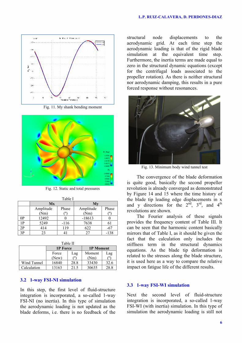
First the case of the uninstalled propeller with rigid blades is considered. The CFD simulation is advanced in a time-accurate mode during at least three complete propeller rotations to achieve convergence. Figures 10 and 11 show the time evolution during the second and third propeller revolutions of the two components of the blade shank bending moments Mx (propeller disk in-plane bending moment) and My (propeller disk out of plane bending moment). It can be seen that convergence has been effectively achieved. Figure 12 shows a snapshot of the solution at the end of the 3rd revolution. The color code on the blades corresponds to the static pressure, whereas the color code on the back plane represents the ratio of local total pressure to free-stream total pressure. The different aerodynamic environment of the blade down and blade up sides of the propeller due to the incidence effect can be clearly seen.

A Fourier analysis of the last revolution results in the frequency content of Table I. It can be seen that the 1P component is the main contributor to the blade vibrations, its value being of similar order of magnitude than the stationary load, whereas the higher harmonics are significantly smaller.

Composition of the forces and moments acting on the 8 blades provides the shaft loads. The different blades compensate each other resulting in stationary loads and moments. The x components of the forces and moments, that is, the thrust and the torque are known from the

propeller deck, so they provide a good opportunity to gauge the accuracy of the CFD calculation.

For the particular condition calculated here the thrust calculated by the CFD model is just 1% above the propeller deck value, whereas the torque prediction is 5% above the propeller deck values. The slightly degraded accuracy of the torque is normal given the fact that it mainly derives from the drag components of the blade whereas the thrust is mostly determined by the lift component. The y and z components of the loads, that is, the in-plane loads on the shaft are known as the 1P loads and moments, they are typically presented in terms of a total 1P load or moment plus a lag angle with respect to the z-axis. For the uninstalled propeller these loads have been measured in the wind tunnel using rotary shaft balances (Figures 13). The propellers used in the wind tunnel models are very rigid (they are manufactured out of carbon fiber) so the measured 1P forces and moments provide an additional opportunity for the validation of the rigid blade calculations. Table II shows a comparison of the experimental and calculated 1P forces and moments. It can be seen that the comparison is not as good as that achieved for the torque and thrust. This is somehow surprising as these loads and moments are the result of the same pressures and friction coefficients on the blades that generate the thrust and torque. The fact that even though the CFD analysis slightly over-predicts the thrust and torque it under predicts the 1P load and moment is an indication that inaccuracies in the wind tunnel data may be also playing a role.

Fig. 10. Mx shank bending moment


6

Fig. 11. My shank bending moment

Fig. 12. Static and total pressures

Table I

Mx My Amplitude

(Nm) Phase

(º) Amplitude

(Nm) Phase

(º) 0P 12492 0 -18613 0 1P 5249 -116 7638 61 2P 414 119 622 -67 3P 23 41 27 -138

Table II

1P Force 1P Moment Force (New)

Lag (º)

Moment (Nm)

Lag (º)

Wind Tunnel 16840 28.8 33430 32.6 Calculation 13163 21.5 30635 28.8

3.2 1-way FSI-NI simulation

In this step, the first level of fluid-structure integration is incorporated, a so-called 1-way FSI-NI (no inertia). In this type of simulation the aerodynamic loading is not updated as the blade deforms, i.e. there is no feedback of the

structural node displacements to the aerodynamic grid. At each time step the aerodynamic loading is that of the rigid blade simulation at the equivalent time step. Furthermore, the inertia terms are made equal to zero in the structural dynamic equations (except for the centrifugal loads associated to the propeller rotation). As there is neither structural nor aerodynamic damping, this results in a pure forced response without resonances.

Fig. 13. Minimum body wind tunnel test

The convergence of the blade deformation

is quite good, basically the second propeller revolution is already converged as demonstrated by Figure 14 and 15 where the time history of the blade tip leading edge displacements in x and y directions for the 2nd, 3rd, and 4th revolutions are shown.

The Fourier analysis of these signals provides the frequency content of Table III. It can be seen that the harmonic content basically mirrors that of Table I, as it should be given the fact that the calculation only includes the stiffness term in the structural dynamics equations. As the blade tip deformation is related to the stresses along the blade structure, it is used here as a way to compare the relative impact on fatigue life of the different results.

3.3 1-way FSI-WI simulation

Next the second level of fluid-structure integration is incorporated, a so-called 1-way FSI-WI (with inertia) simulation. In this type of simulation the aerodynamic loading is still not

7


updated but now the inertia terms are considered in the structural dynamic simulation and there is the possibility of resonance. As the aerodynamic and structural damping are still zero it corresponds to undamped dynamic magnification.

Fig 14. Tip leading edge x-displacement

Fig 15. Tip leading edge y-displacement

Table III

Tip LE x- displacement

Frequency Amplitude (mm)

Phase (º)

0P -23.4 0.00 1P 17.7 57 2P 1.08 -66 3P 0.07 -178

Tip LE y- displacement


Phase (º)

0P -15.7 0.00 1P 15.6 57 2P 0.95 -65 3P 0.06 -178

Given the higher dynamics of the blade for this case, the convergence of the blade deformation is more difficult than for the previous case, as shown in Figure 16 and 17 where the time history of the blade tip leading edge displacements in x and y directions is compared for the 2nd to 5th revolutions.



The Fourier analysis of the last revolution

results in the frequency content of Table IV. It can be readily seen that the 2P harmonic has increased very significantly, with a dynamic magnification factor of 13.5. This is a direct consequence of the fact that the take-off rotational speed of the propeller is very close to a critical speed for the first flatwise bending mode of the blade as shown in Figure 8, so that the 2P content of the aerodynamic loads in Table I, even though it is very small, generates large oscillation amplitudes. The 1P and 3P excitations, are more separated from the


8

resonance frequency, so their dynamic amplification is much smaller, namely 1.3 for the 1P, and 4.7 for the 3P (although it is worth noting that for the 3P the figures have to be taken with caution as they result from very small numbers).

Table IV Tip LE x- displacement


Phase (º)

0P -23.4 0.00 1P 22.7 57 2P 14.6 -83 3P 0.32 87



Phase (º)

0P -15.6 0.00 1P 20.2 57 2P 13.03 -83 3P 0.29 78

3.4 2-way FSI simulation

The final step is the fully coupled fluid-structure simulation. Now the aerodynamic loading is updated as the blade deforms. The structural nodes displacements are transferred to the aerodynamic grid and it is deformed accordingly. The consequence is twofold: the aerodynamic loads are modified; and aerodynamic damping is introduced into the structure dynamics.

Figures 18 and 19 show the time history of the blade tip leading edge displacements in x and y directions for the 2nd, 3rd, and 4th revolutions. The convergence is quite rapid again thanks to the smoothing effect of the aerodynamic damping.

Table V presents the frequency content of the last propeller revolution. It can be seen that the aerodynamic damping significantly reduces the 2P and 3P content. For the 2P response the damping factor is 2.5. On the other hand, the 1P response is slightly amplified by a factor of 1.02, the so-called twist magnification, which for this case is small due to the fact that the first flatwise bending mode has a reduced torsion component.

The aerodynamic loads acting on the blades are summarized in Table VI. Comparison

between Tables I and VI shows that interaction with the structure slightly increases the 1P component and reduces the 2P component due to aerodynamic damping. Even though the 2P loading is decreased the 2P vibrations are still larger than those in Table III due to the dynamic amplification.



Table V

Tip LE x-displacement


Phase (º)

0P -23.5 0.00 1P 23.3 44 2P 5.8 -161 3P 0.03 -126



Phase (º)

0P -15.8 0.00 1P 20.6 45 2P 5.14 -161 3P 0.04 -129

9


Table VI Mx My Amplitude

(Nm) Phase

(º) Amplitude

(Nm) Phase

(º) 0P 12369 0 -18618 0 1P 5239 -123 7791 61 2P 159 99 241 -67 3P 11 -107 29 -138

Composition of the forces and moments acting on the 8 blades results in the shaft loads of Table VII. Comparison with Table II shows that inclusion of blade deformation produces a small increment of these loads.

Table VII 1P Force 1P Moment

Force (New)

Lag (º)

Moment (Nm)

Lag (º)

Calculation 13313 25.4 31214 40.4

4 Results. Installed propellers

4.1 Rigid Blade simulation

As for the uninstalled propeller, the first step is a pure CFD simulation with rigid blades. The calculation is performed in a time-accurate mode with the propellers physically rotating with respect to the aircraft. The solution is advanced during three complete propeller revolutions to achieve convergence of the results. Figure 20 shows as an example a snapshot of the results in terms of pressure coefficient.

Fig 20. Installed propellers CFD calculation

The Fourier analysis of the last propeller revolution provides the aerodynamic loads on the blades summarized in Tables VIII and IX

respectively for the inboard and outboard propellers.

Table VIII. Inboard Propeller Mx My Amplitude

(Nm) Phase

(º) Amplitude

(Nm) Phase

(º) 0P 12686 0 -19024 0 1P 5366 -126 7760 49 2P 404 41 622 -148 3P 127 -90 124 85

Table IX. Outboard Propeller

Mx My Amplitude

(Nm) Phase

(º) Amplitude

(Nm) Phase

(º) 0P -12804 0 -19247 0 1P 5430 65 8021 62 2P 1016 -43 1568 -45 3P 184 -126 349 -125

Comparison of Tables I, VIII and IX allow reaching the following conclusions about the installation effects on the blade loads. • There is a small increase of the 0P and 1P

which is similar for both inboard and outboard propellers.

• The 2P loads on the outboard propeller show a tremendous increment in relation to those of the uninstalled propeller (of the order of 250%). On the other hand, the 2P loads on the inboard propeller remain basically unchanged. The reason for the different trend between the outboard and the inboard propellers lies in the opposite sense of rotation. For the outboard propeller the blade-down movement (which corresponds to the maximum loads on the blade) is closer to the wing leading edge than the blade-up part and is thus in a region of higher flow distortion, creating stronger differences in the blade loading from one side to the other. For the inboard propeller the opposite holds true.

• The flow distortion significantly increases the 3P content for both propellers.

The resulting shaft loads are summarized

in Tables X and XI where they are compared with the data from the wind tunnel tests of Figure 9. It can be seen that, as was the case for the uninstalled propeller in Table II, the calculation still underestimates the 1P loads and


10

moments, but it correctly captures the increment associated to the installation effect.

Table X. Inboard Propeller 1P Force 1P Moment

Force (New)

Lag (º)

Moment (Nm)

Lag (º)

Wind Tunnel 17485 28.3 34286 32.3 Calculation 14190 29.8 30749 41.12

Table XI. Outboard Propeller 1P Force 1P Moment

Force (New)

Lag (º)

Moment (Nm)

Lag (º)

Wind Tunnel 17565 -18.7 34453 157 Calculation 14103 -20.24 31698 150

4.2 1-way FSI-WI simulation

The installed propellers computation is very expensive computationally, so the fluid-structure interaction simulation has been limited to the 1-way FSI with inertia case, which is to be compared with that of section 3.3 for the uninstalled propeller.

Figures 21 to 24 present the time history of the blade tip leading edge displacements for both propellers. It can be seen that in this case it takes much longer to achieve a reasonable level of convergence. Tables XII and XIII respectively present the frequency content of the last propeller revolution for the inboard and outboard propellers.

Fig. 21. Inboard Propeller. Tip x-displacement

Fig. 22. Inboard Propeller. Tip y-displacement

Fig. 23. Outboard Propeller. Tip x-displacement

Fig. 24. Outboard Propeller. Tip y-displacement

Comparison with Table IV show the very

important increment in the 2P component due to the installation effect, which is in line with the increments in the blade loads obtained in the previous section. It is worth noting that for the outboard propeller the 2P component is the dominant one, even larger than the 0P and 1P components. The very high dynamics of this case explain the difficulties encountered in achieving convergence.

11


Table XII. Inboard Propeller Tip LE x-displacement


Phase (º)

0P -21.8 0.00 1P 20.7 45 2P 20.2 -172 3P 1.2 34



Phase (º)

0P -15.9 0.00 1P 19.8 46 2P 19.2 -172 3P 1.1 32

Table XIII. Outboard Propeller

Tip LE x-displacement


Phase (º)

0P -23.0 0.00 1P 23.0 55 2P 58.8 -60 3P 2.3 90



Phase (º)

0P 15.3 0.00 1P 20.5 -125 2P 53.0 120 3P 2.2 -93

5 Conclusions

This study has investigated the potential of CFD-CSM coupling to predict both the static loads and vibration environment of installed propellers including aeroelastic effects and without the need to incorporate the simplifying assumptions typically used in this type of analysis.

When the propeller is installed on a swept wing there are important interference effects between the propeller blades and the wing leading edge. These effects depend on the sense of rotation of the propeller.

Special care must be applied when it has not been possible to achieve a large margin between the blade natural frequencies and the 2nd harmonic of the propeller rotational speed, as it can generate very large oscillatory loads

that may become the main contributors to the propeller fatigue life consumption.

References

[1] Sullivan, W. E.; Turnberg, J. E.; Violette, J. A.; “Large-Scale Advanced-Propfan (LAP) Blade Design” NASA CR 174970;

[2] FAA; “Vibration and Fatigue Evaluation of Airplane Propellers”; AC-20-66A; 2001

[3] McCormick, B. W. Jr.; “Aerodynamics of V/STOL Flight”; Academic Press, 1967

[4] ANSYS-CFX Theory Guide [5] ANSYS Mechanical APDL Guide – Theory

Reference. [6] ANSYS Mechanical APDL Guide – Coupled field

analysis guide.

Copyright Statement

The authors confirm that they, and/or their company or organization, hold copyright on all of the original material included in this paper. The authors also confirm that they have obtained permission, from the copyright holder of any third party material included in this paper, to publish it as part of their paper. The authors confirm that they give permission, or have obtained permission from the copyright holder of this paper, for the publication and distribution of this paper as part of the ICAS2012 proceedings or as individual off-prints from the proceedings.

cfd based aeroelastic calculation of propeller loads

Documents