aerosol penetration of leak pathways – an examination of ... · u.s. department of commerce ......
TRANSCRIPT
SANDIA REPORT SAND2009-1701 Unlimited Release Printed April 2009
Aerosol Penetration of Leak Pathways – An Examination of the Available Data and Models Dana A. Powers Prepared by Sandia National Laboratories Albuquerque, New Mexico 87185 and Livermore, California 94550 Sandia is a multiprogram laboratory operated by Sandia Corporation, a Lockheed Martin Company, for the United States Department of Energy’s National Nuclear Security Administration under Contract DE-AC04-94AL85000. Approved for public release; further dissemination unlimited.

2
Issued by Sandia National Laboratories, operated for the United States Department of Energy by Sandia Corporation. NOTICE: This report was prepared as an account of work sponsored by an agency of the United States Government. Neither the United States Government, nor any agency thereof, nor any of their employees, nor any of their contractors, subcontractors, or their employees, make any warranty, express or implied, or assume any legal liability or responsibility for the accuracy, completeness, or usefulness of any information, apparatus, product, or process disclosed, or represent that its use would not infringe privately owned rights. Reference herein to any specific commercial product, process, or service by trade name, trademark, manufacturer, or otherwise, does not necessarily constitute or imply its endorsement, recommendation, or favoring by the United States Government, any agency thereof, or any of their contractors or subcontractors. The views and opinions expressed herein do not necessarily state or reflect those of the United States Government, any agency thereof, or any of their contractors. Printed in the United States of America. This report has been reproduced directly from the best available copy. Available to DOE and DOE contractors from U.S. Department of Energy Office of Scientific and Technical Information P.O. Box 62 Oak Ridge, TN 37831 Telephone: (865) 576-8401 Facsimile: (865) 576-5728 E-Mail: [email protected] Online ordering: http://www.osti.gov/bridge Available to the public from U.S. Department of Commerce National Technical Information Service 5285 Port Royal Rd. Springfield, VA 22161 Telephone: (800) 553-6847 Facsimile: (703) 605-6900 E-Mail: [email protected] Online order: http://www.ntis.gov/help/ordermethods.asp?loc=7-4-0#online

3
SAND2009-1701 Unlimited Release
April 2009
Aerosol Penetration of Leak Pathways – An Examination of the Available Data and Models
Dana A. Powers 6770 Advanced Nuclear Energy Programs
Sandia National Laboratories P.O. Box 5800
Albuquerque, New Mexico 87185-MS0748
Abstract
Data and models of aerosol particle deposition in leak pathways are described. Pathways considered include capillaries, orifices, slots and cracks in concrete. The Morewitz-Vaughan criterion for aerosol plugging of leak pathways is shown to be applicable only to a limited range of particle settling velocities and Stokes numbers. More useful are sampling efficiency criteria defined by Davies and by Liu and Agarwal. Deposition of particles can be limited by bounce from surfaces defining leak pathways and by resuspension of particles deposited on these surfaces. A model of the probability of particle bounce is described. Resuspension of deposited particles can be triggered by changes in flow conditions, particle impact on deposits and by shock or vibration of the surfaces. This examination was performed as part of the review of the AP1000 Standard Combined License Technical Report, APP-GW-GLN-12, Revision 0, “Offsite and Control Room Dose Changes” (TR-112) in support of the USNRC AP1000 Standard Combined License Pre-Application Review.

4
5
CONTENTS
1. INTRODUCTION ........................................................................................................ 11
2. EXPERIMENTAL STUDIES ...................................................................................... 19 2.1 Leak Pathway Idealizations .......................................................................................... 19
2.1.1 Capillary Flow ................................................................................................ 20 2.1.2 Orifice Flow .................................................................................................... 22 2.1.3 Flow in Slots ................................................................................................... 23 2.1.4 Concrete Cracks .............................................................................................. 23 2.1.5 Gasket Leaks ................................................................................................... 29
2.2 Individual Experimental Studies ................................................................................... 31 2.2.1 Experiments with Capillaries by Mitchell and Coworkers ............................. 31 2.2.2 Capillary Tests by Nelson and Johnson .......................................................... 36 2.2.3 Tests of Depleted Uranium Dioxide Flow Through Capillaries. .................... 37 2.2.4 Rockwell Tests on Capillary Flow .................................................................. 45 2.2.5 Tests with Orifices .......................................................................................... 47 2.2.6 Lewis Tests of Particle Transport Through a Slot .......................................... 62 2.2.7 Mosley et al. Tests of Aerosol Transport Through a Slot ............................... 64 2.2.8 Liu and Nazaroff Tests of Aerosol Flow Through Slots ................................. 67 2.2.9 Tests with Cracked Concrete .......................................................................... 70 2.2.10 Tests of Leakage from a Flow Stream ............................................................ 75 2.2.11 Multiple Bend Geometry Tests ....................................................................... 77 2.2.12 Tests of Leakage Through Containment Penetrations .................................... 77 2.2.13 Containment Leak Tests ................................................................................. 78
2.3 Turbulent Deposition of Particles ................................................................................. 79 2.3.1 Friedlander and Johnstone .............................................................................. 81 2.3.2 Montgomery and Corn .................................................................................... 82 2.3.3 Wells and Chamberlain ................................................................................... 83 2.3.4 Liu and Agarwal ............................................................................................. 84 2.3.5 El-Shobokshy .................................................................................................. 85 2.3.6 Lee and Gieseke .............................................................................................. 85 2.3.7 Shimada et al. .................................................................................................. 86 2.3.8 Sehmel............................................................................................................. 87 2.3.9 Postma and Schwendiman .............................................................................. 88 2.3.10 Ilori .................................................................................................................. 89 2.3.11 Muyshondt et al............................................................................................... 90 2.3.12 Forney and Spielman ...................................................................................... 91
3. THEORETICAL INVESTIGATIONS ........................................................................ 93 3.1 Laminar Flow Conditions ............................................................................................. 93 3.2 Chen Yu Method for Deposition by Multiple Mechanisms .......................................... 97 3.3 Turbulent Flow Conditions ......................................................................................... 101 3.4 Other Considerations .................................................................................................. 105
4. CONCLUSIONS ........................................................................................................ 109

6
5. REFERENCES ........................................................................................................... 111
Appendix A: DERIVATION OF THE STOKES NUMBER .................................................... 117
Appendix B: TABULATED DATA ON TURBULENT DEPOSITION OF AEROSOL PARTICLES IN SMOOTH TUBES .......................................................................................... 121

7
FIGURES
Figure 1. Data Cited by Morewitz [1982] for His Simple Correlation. ....................................... 12Figure 2. Data Cited by Vaughan [1978] for His Simple Correlation. ........................................ 12Figure 3. Regimes for Aerosol Transport in Sampling Devices. ................................................. 15Figure 4. Commercial Aerosol Sampling Device Characteristics in Terms of Agarwal and Liu Sampling Regimes. ....................................................................................................................... 15Figure 5. Sampling Efficiency Data [Yoshida et al., 1979] and the Agarwal and Liu “Pretty Good” Sampling Regime. ............................................................................................................. 16Figure 6. Leak Pathway Idealizations. ......................................................................................... 19Figure 7. Crack Dimensions. ....................................................................................................... 26Figure 8. Cracks Produced in Concrete by Predominantly Membrane Stress. ............................ 27Figure 9. Concrete Cracks Produced by Membrane and Shear Stress at a Penetration. .............. 28Figure 10. Size Distribution of Glass Sphere Aerosols Used in Tests by Mitchell and Coworkers.
....................................................................................................................................................... 33Figure 11. Flow Through Capillaries Exposed to Glass Sphere Aerosol. ................................... 33Figure 12. Number of Particles that Emerged from Capillaries After 2 Hours. .......................... 34Figure 13. Comparison of Probability Density Function for the Number Distributions of Aerosol Input and Exiting from a 5 cm long 70 µm Capillary. .................................................................. 34Figure 14. Flow Characteristics of Capillaries Used by Sutter et al. [Owzarski et al., 1979]. .... 39Figure 15. Comparison of Observed Transmission of Uranium Dioxide Powder Through Capillaries in Tests Reported by Sutter et al with Transmission Expected if Penetration Through Capillaries was 100%. ................................................................................................................... 43Figure 16. Comparison of Observed [Sutter et al., 1980] Uranium Dioxide Powder Leakage Through Orifices Plotted Against the Expected Leakage Assuming 100% Particle Penetration of the Orifice. .................................................................................................................................... 47Figure 17. Lewis [1995] results for aerosol flow through a 0.1 mm slot at a pressure differential of 10 kPa. ...................................................................................................................................... 62Figure 18. Results of Tests by Mosley et al. [2001] for Aerosol Transport Through a Slot 0.5 mm High, 433 mm Wide, and 102 mm Deep at a 2 kPa Differential Pressure ............................ 65Figure 19. Results of Tests by Mosley et al. [2001] for Aerosol Transport Through a Slot 0.5 mm High, 433 mm Wide, and 102 mm Deep at a 5 kPa Differential Pressure ............................ 65Figure 20. Results of Tests by Mosley et al. [2001] for aerosol transport through a slot 0.5 mm high, 433 mm wide, and 102 mm deep at a 10 kPa Differential Pressure .................................... 66Figure 21. Results of Tests by Mosley et al. [2001] for Aerosol Transport Through a Slot 0.5 mm High, 433 mm Wide, and 102 mm Deep at a 20 kPa Differential Pressure .......................... 66Figure 22. Data from Liu and Nazaroff for Aerosol Flow Through a slot 0.25 mm high and 9.4 cm deep at a 2 Pa Differential Pressure ........................................................................................ 68Figure 23. Data from Liu and Nazaroff for Aerosol Flow Through a slot 0.25 mm high and 9.4 cm deep at a 10 Pa Differential Pressure ...................................................................................... 68Figure 24. Data from Liu and Nazaroff for Aerosol Flow Through a slot 0.25 mm high and 4.3 cm deep at a 10 Pa Differential Pressure ...................................................................................... 69Figure 25. Data from Liu and Nazaroff for Aerosol Flow Through a slot 1.0 mm high and 9.4 cm deep at a 10 Pa Differential Pressure ...................................................................................... 69

8
Figure 26. Penetration of Uranine Particles Through a 67.2 µm Crack in Concrete [Gelain and Vendel, 2008]. ............................................................................................................................... 74Figure 27. Carrié and Modera [1998] on the Variation in Slot Height Due to Aerosol Accumulation from Transverse Flow. .......................................................................................... 76Figure 28. Comparison of Leakage Flow of Aerosol-Laden Gas Through a Slot and a Joint [Carrié and M.P. Modera, 2002]. .................................................................................................. 76Figure 29. Turbulent Aerosol Particle Deposition Data Obtained by Friedlander and Johnstone [1957]. ........................................................................................................................................... 81Figure 30. Turbulent Particle Deposition Reported by Montgomery and Corn [1970]. .............. 82Figure 31. Turbulent Deposition of Tricresyl Phosphate Droplets [Wells and Chamberlain, 1967]. ............................................................................................................................................ 83Figure 32. Turbulent Particle Deposition Data from Liu and Agarwal [1974 ] and from El-Shobokshy [1983]. ........................................................................................................................ 84Figure 33. Turbulent Deposition Velocities for Dioctyl Phthalate Droplets [Lee and Gieseke, 1994]. ............................................................................................................................................ 85Figure 34. Turbulent NaCl Aerosol Deposition Data from Shimada et al. [1993]. ..................... 86Figure 35. Data on the Turbulent Deposition of Uranine Particles Obtained by Sehmel [1970]. 87Figure 36. Turbulent Aerosol Deposition Data from Postma and Schwendiman [1960]. ........... 88Figure 37. Turbulent Particle Deposition Data Obtained by Ilori in His Thesis Research. Data Digitized from a Small Plot Published by Im and Ahluwalia [1989]. .......................................... 89Figure 38. Turbulent Deposition of Oleic Acid Droplets [Muyshondt et al., 1996]. .................. 90Figure 39. Data on Turbulent Deposition of Large Particles [Forney and Spielman, 1974]. ...... 91Figure 40. Turbulent Particle Deposition Data from Several Investigations. .............................. 92Figure 41. Comparison of a Model of Particle Bounce Probability to Data on the Bounce of Fly Ash Particles from Filter Beds. ................................................................................................... 107

9
TABLES
Table 1. Glass Aerosol Deposition in a Capillary with a Pressure Differential of 40 kPa. ......... 35Table 2. Results of Tests by Mitchell and Coworkers. ................................................................ 35Table 3. Continued Gas Flow Through Capillaries Following Plugging in Tests by Mitchell and Coworkers. .................................................................................................................................... 36Table 4. Results From Tests with Sodium Oxide and Sodium Hydroxide Aerosols Reported by Nelson and Johnson [1975]. .......................................................................................................... 37Table 5. Characteristics of Capillaries Used by Sutter et al. ....................................................... 39Table 6. Flow Characteristics [Owzarski et al., 1979] of Capillaries Used by Sutter et al. ........ 40Table 7. Results of Tests by Sutter et al. with Capillaries ........................................................... 41Table 8. Parametric Values for Capillaries. ................................................................................. 44Table 9. Capillary Plugging Results Reported by Rockwell International [1997]. ..................... 46Table 10. Data Reported by Sutter et al. for Air-Sparged Uranium Dioxide Transmission Through Orifices. .......................................................................................................................... 48Table 11. Parametric Values for Orifices. ................................................................................... 61Table 12. Some Results of Experiments by Mitchell et al. [1992] on the Penetration of Orifices by Nominally 7 µm glass Aerosol Particles. ................................................................................. 61Table 13. Results of Lewis’ Test [1995] of Particle Transport Through a Slot (Best Fit Results).
....................................................................................................................................................... 63Table 14. Results of Lewis’ Test [1995] of Particle Transport Through a Slot (Data for Talc Particles). ...................................................................................................................................... 63Table 15. Penetration Observed in Transport of Polystyrene Latex Aerosols Through Cracks in Concrete [van de Vate, 1988]. ...................................................................................................... 72Table 16. Uranine Particle Penetration of Cracks (h = 67.2 µm) in Concrete [Gelain and Vendel, 2008]. ............................................................................................................................. 73Table 17. Comparison of Williams Turbulent Deposition Model to Results of Tests by Nelson and Johnson. ................................................................................................................................ 103Table B-1. Tablulated Data from Investigations by Forney and Spielman Using Tubes Coated with a Mixture of 75% Paraffin Oil and 25% Petroleum Jelly to Suppress Particle Bounce. .... 122Table B-2. Tabulated Data from Investigations by Friedlander and Johnstone. ....................... 123Table B-3. Tabulated data from investigations by Ilori. ............................................................ 124Table B-4. Tabulated data from investigations by Lee and Gieseke. ........................................ 125Table B-5. Tabulated Data from Investigations by Liu and Agarwal. ....................................... 126Table B-6. Tabulated Data from Investigations by Montgomery and Corn. ............................. 127Table B-7. Tabulated Data from Investigations by Muyshondt et al. ....................................... 128Table B-8. Tabulated Data from Investigations by Postma and Swendiman. ........................... 129Table B-9. Tabulated Data from Investigations by Shimada, Okayama, and Asai. .................. 130Table B-10. Tabulated Data from Investigations by Shobokshy. .............................................. 131Table B-11. Tabulated Data from Investigations by Wells and Chamberlain. .......................... 132Table B-12. Tabulated Data from Investigations by Sehmel. .................................................... 133

10

11
1. INTRODUCTION The phenomena associated with radioactive aerosol penetration of narrow leakage pathways have been issues of reactor safety at least since the establishment of the siting criteria in 10 CFR Part 100. The issues of aerosol leakage arise in connection with cracking of concrete containments, bypass of valves, perforation of electrical penetrations, and failure of seals such as those between the drywells and wetwells of boiling water reactors. The consequences of leakage of radioactive aerosol affect siting suitability, risk assessment and control room habitability. More recently, aerosol penetration of leak paths has been discussed in connection with dry cask storage of spent nuclear fuel and transportation of radioactive materials in casks. Aerosol transport through narrow passages gained great visibility during the late 1970s in connection with the safety analysis of liquid metal fast breeder reactors (LMFBRs). The emphasis of these discussions was on sodium fires that produce enormous amounts of radioactive aerosol. There was, however, also some interest in aerosols produced during energetic power excursions of reactor fuel. Such events can produce quite large amounts of radioactive aerosol by vaporizing the fuel. Within this context, Morewitz [1982], Morewitz et al.[1979] and Vaughan [1978] provided an extraordinarily simple model to predict aerosol transport through passages: 3
ductkDm = (1) where
m - aerosol mass transport through a passage prior to plugging (kg) ductD - equivalent diameter of the leak pathway (m)
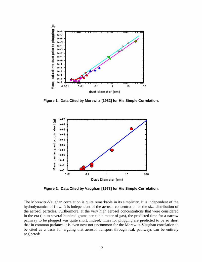
k - constant = (5±3)×104 (kg/m3) Plots of data used by Morewitz and by Vaughan to support the simple correlation are shown in Figure 1 and Figure 2, respectively. Note that plugging was understood to mean obstruction of the plow pathway sufficient to filter aerosol from the gas stream. It did not mean a leak tight seal on the pathway, though especially in tests with very hygroscopic aerosol such as NaOH, leaktight plugging might be observed.
12
Figure 1. Data Cited by Morewitz [1982] for His Simple Correlation.
Figure 2. Data Cited by Vaughan [1978] for His Simple Correlation.
The Morewitz-Vaughan correlation is quite remarkable in its simplicity. It is independent of the hydrodynamics of flow. It is independent of the aerosol concentration or the size distribution of the aerosol particles. Furthermore, at the very high aerosol concentrations that were considered in the era (up to several hundred grams per cubic meter of gas), the predicted time for a narrow pathway to be plugged was quite short. Indeed, times for plugging are predicted to be so short that in common parlance it is even now not uncommon for the Morewitz-Vaughan correlation to be cited as a basis for arguing that aerosol transport through leak pathways can be entirely neglected!
13
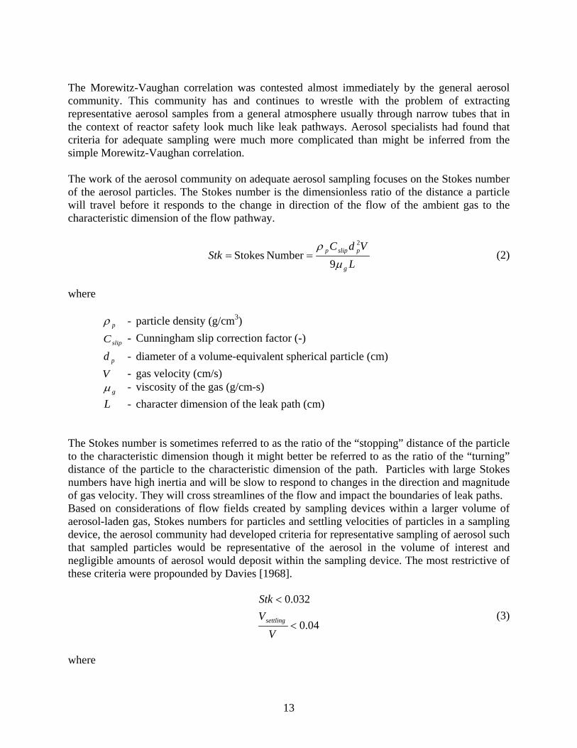
The Morewitz-Vaughan correlation was contested almost immediately by the general aerosol community. This community has and continues to wrestle with the problem of extracting representative aerosol samples from a general atmosphere usually through narrow tubes that in the context of reactor safety look much like leak pathways. Aerosol specialists had found that criteria for adequate sampling were much more complicated than might be inferred from the simple Morewitz-Vaughan correlation. The work of the aerosol community on adequate aerosol sampling focuses on the Stokes number of the aerosol particles. The Stokes number is the dimensionless ratio of the distance a particle will travel before it responds to the change in direction of the flow of the ambient gas to the characteristic dimension of the flow pathway.
L
VdCStk
g
pslipp
µρ
9Number Stokes
2
== (2)
where
pρ - particle density (g/cm3)
slipC - Cunningham slip correction factor (-)
pd - diameter of a volume-equivalent spherical particle (cm) V - gas velocity (cm/s)
gµ - viscosity of the gas (g/cm-s) L - character dimension of the leak path (cm)
The Stokes number is sometimes referred to as the ratio of the “stopping” distance of the particle to the characteristic dimension though it might better be referred to as the ratio of the “turning” distance of the particle to the characteristic dimension of the path. Particles with large Stokes numbers have high inertia and will be slow to respond to changes in the direction and magnitude of gas velocity. They will cross streamlines of the flow and impact the boundaries of leak paths. Based on considerations of flow fields created by sampling devices within a larger volume of aerosol-laden gas, Stokes numbers for particles and settling velocities of particles in a sampling device, the aerosol community had developed criteria for representative sampling of aerosol such that sampled particles would be representative of the aerosol in the volume of interest and negligible amounts of aerosol would deposit within the sampling device. The most restrictive of these criteria were propounded by Davies [1968].
04.0
032.0
<
<
VVStk
settling (3)
where
14
settlingV - χµ
ρ18
2 gdC pslipp
g - terrestrial gravitational acceleration (cm/s2) χ - dynamic shape factor (vida infra)
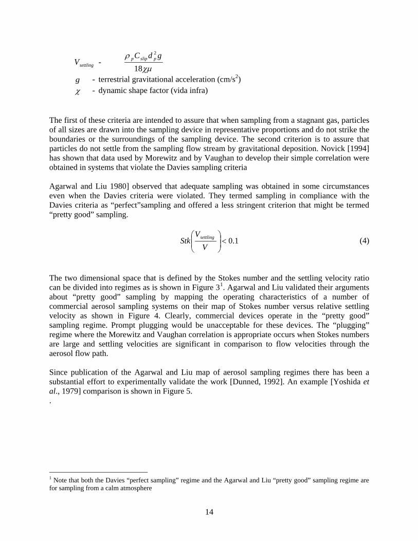
The first of these criteria are intended to assure that when sampling from a stagnant gas, particles of all sizes are drawn into the sampling device in representative proportions and do not strike the boundaries or the surroundings of the sampling device. The second criterion is to assure that particles do not settle from the sampling flow stream by gravitational deposition. Novick [1994] has shown that data used by Morewitz and by Vaughan to develop their simple correlation were obtained in systems that violate the Davies sampling criteria Agarwal and Liu 1980] observed that adequate sampling was obtained in some circumstances even when the Davies criteria were violated. They termed sampling in compliance with the Davies criteria as “perfect”sampling and offered a less stringent criterion that might be termed “pretty good” sampling.
1.0<
V
VStk settling (4)
The two dimensional space that is defined by the Stokes number and the settling velocity ratio can be divided into regimes as is shown in Figure 31
Figure 4
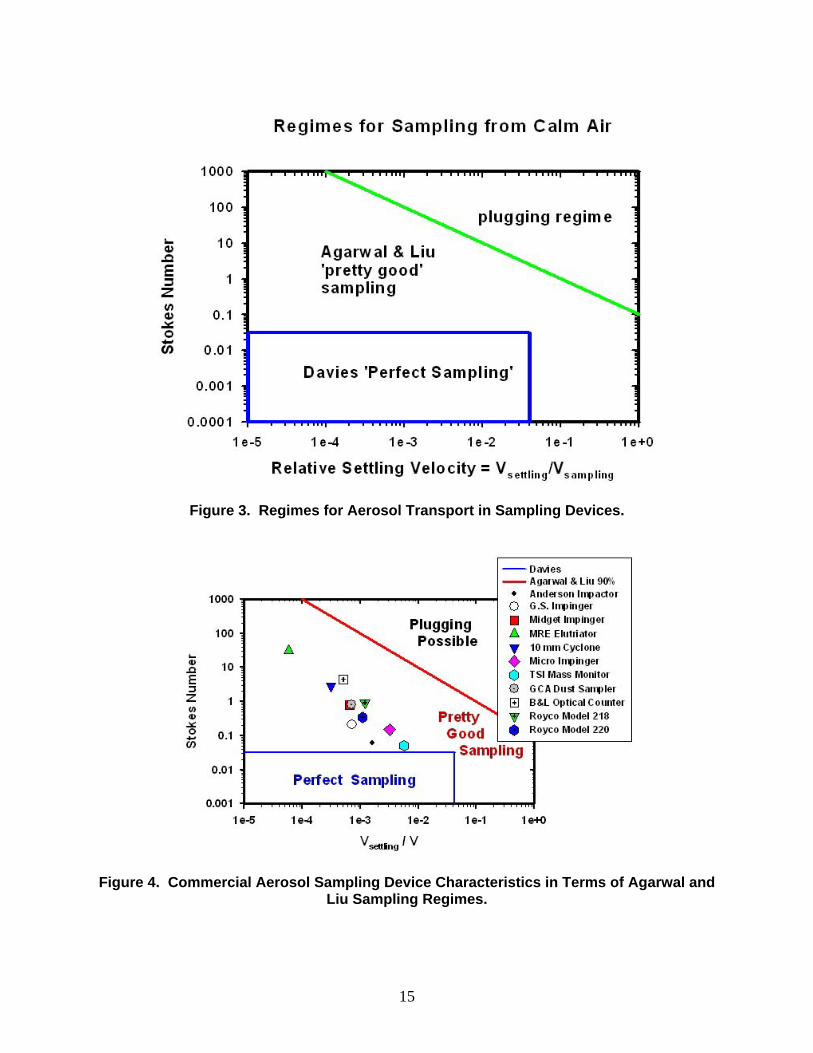
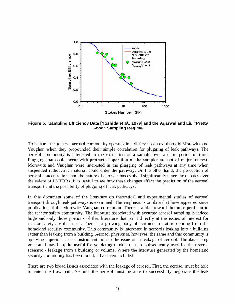
. Agarwal and Liu validated their arguments about “pretty good” sampling by mapping the operating characteristics of a number of commercial aerosol sampling systems on their map of Stokes number versus relative settling velocity as shown in . Clearly, commercial devices operate in the “pretty good” sampling regime. Prompt plugging would be unacceptable for these devices. The “plugging” regime where the Morewitz and Vaughan correlation is appropriate occurs when Stokes numbers are large and settling velocities are significant in comparison to flow velocities through the aerosol flow path. Since publication of the Agarwal and Liu map of aerosol sampling regimes there has been a substantial effort to experimentally validate the work [Dunned, 1992]. An example [Yoshida et al., 1979] comparison is shown in Figure 5. .
1 Note that both the Davies “perfect sampling” regime and the Agarwal and Liu “pretty good” sampling regime are for sampling from a calm atmosphere
15
Figure 3. Regimes for Aerosol Transport in Sampling Devices.
Figure 4. Commercial Aerosol Sampling Device Characteristics in Terms of Agarwal and
Liu Sampling Regimes.
16
Figure 5. Sampling Efficiency Data [Yoshida et al., 1979] and the Agarwal and Liu “Pretty
Good” Sampling Regime. To be sure, the general aerosol community operates in a different context than did Morewitz and Vaughan when they propounded their simple correlation for plugging of leak pathways. The aerosol community is interested in the extraction of a sample over a short period of time. Plugging that could occur with protracted operation of the sampler are not of major interest. Morewitz and Vaughan were interested in the plugging of leak pathways at any time when suspended radioactive material could enter the pathway. On the other hand, the perception of aerosol concentrations and the nature of aerosols has evolved significantly since the debates over the safety of LMFBRs. It is useful to see how these changes affect the prediction of the aerosol transport and the possibility of plugging of leak pathways. In this document some of the literature on theoretical and experimental studies of aerosol transport through leak pathways is examined. The emphasis is on data that have appeared since publication of the Morewitz-Vaughan correlation. There is a bias toward literature pertinent to the reactor safety community. The literature associated with accurate aerosol sampling is indeed huge and only those portions of that literature that point directly at the issues of interest for reactor safety are discussed. There is a growing body of pertinent literature coming from the homeland security community. This community is interested in aerosols leaking into a building rather than leaking from a building. Aerosol physics is, however, the same and this community is applying superior aerosol instrumentation to the issue of in-leakage of aerosol. The data being generated may be quite useful for validating models that are subsequently used for the reverse scenario - leakage from a building or volume. Where the literature generated by the homeland security community has been found, it has been included. There are two broad issues associated with the leakage of aerosol. First, the aerosol must be able to enter the flow path. Second, the aerosol must be able to successfully negotiate the leak

17
pathway and emerge into a surroundings where the radioactivity of the particles could have consequence. The focus of this review is really on the second of these issues. There will always be some deposition of aerosol in a leakage pathway. The amount of deposition and the effects of deposits on the behavior of flow through the path including the formation of plugs are of interest. The next chapter discusses some of the experimental studies and data that are available. The third chapter of this report discusses modeling of the experiments. The final chapter summarizes and draws conclusions concerning the technology now available for predicting aerosol transport through leak paths.

18
19
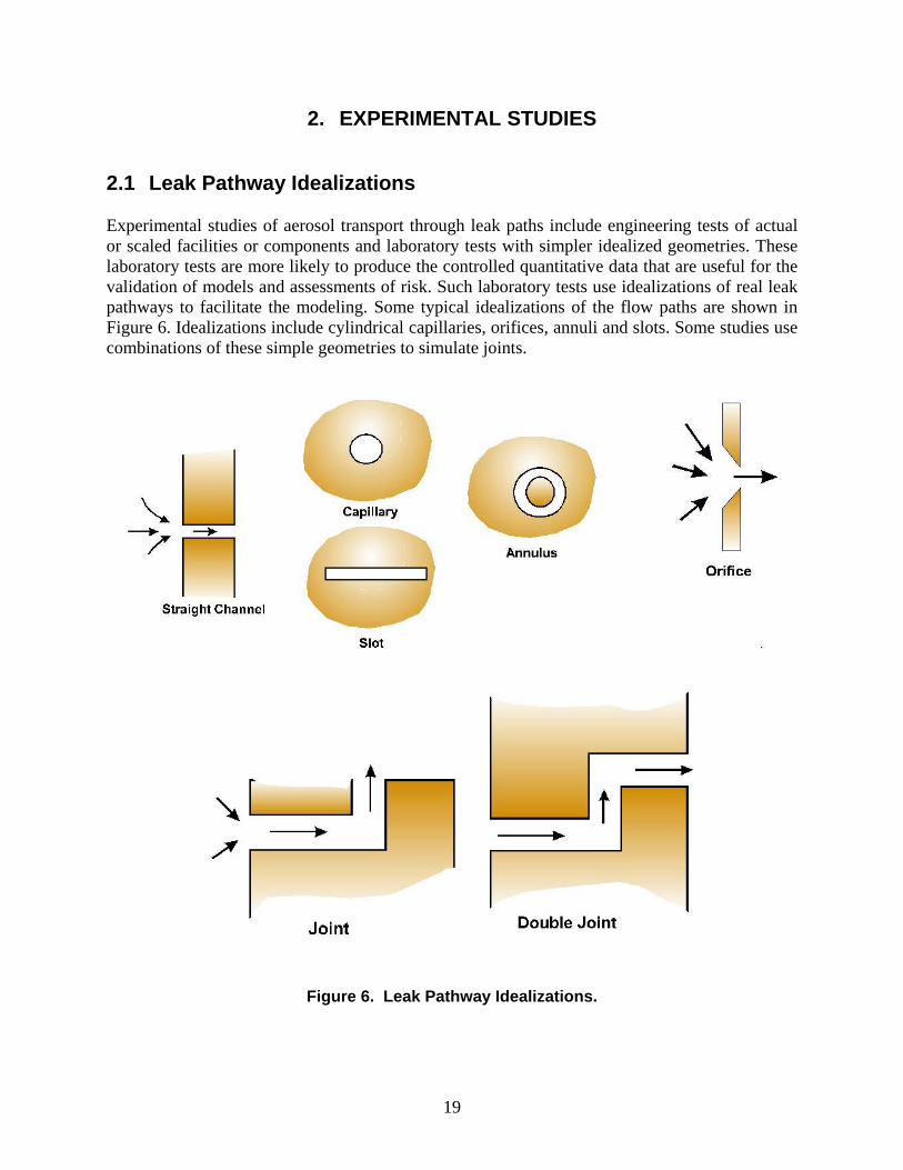
2. EXPERIMENTAL STUDIES 2.1 Leak Pathway Idealizations Experimental studies of aerosol transport through leak paths include engineering tests of actual or scaled facilities or components and laboratory tests with simpler idealized geometries. These laboratory tests are more likely to produce the controlled quantitative data that are useful for the validation of models and assessments of risk. Such laboratory tests use idealizations of real leak pathways to facilitate the modeling. Some typical idealizations of the flow paths are shown in Figure 6. Idealizations include cylindrical capillaries, orifices, annuli and slots. Some studies use combinations of these simple geometries to simulate joints.
Figure 6. Leak Pathway Idealizations.

20
2.1.1 Capillary Flow By far and away the most common idealization is to treat a leak path as a straight cylindrical duct. Laboratory tests for such idealizations dominate the older literature and are particularly appropriate for the study of aerosol sampling adequacy. Cross sections of interest here are larger than 20 µm and typically smaller than about 3500 µm. For such small cross sections, laminar flow or flow approaching the transition between laminar and turbulent flow will be expected. Of course the parabolic velocity profile characteristic of laminar flow does not develop instantaneously. Usually, it is assumed that the parabolic flow profile of laminar flow develops over an entrant region of length Z given by: ReN05.0 hDZ = (5) where
Z - entrance length hD - hydraulic diameter = 4x flow area/wetted perimeter
ReN - Reynolds number The isothermal flow of compressible gas through a long cylindrical capillary is given by the well-known expression [Bird, Stewart, and Lightfoot, 1960]:
DfL
PP
PP
MDRT
low
high
high
low
w
2ln
132
Q
242
2
+
−
=
π
(6)
where
Q - volumetric flow rate D - capillary diameter f - Fanning friction factor L - capillary length
wM - gas molecular weight
highP - inlet pressure
lowP - outlet pressure R - universal gas constant = 83.14472 cm3-bar/mole-K T - absolute temperature

21
To approximate real capillaries that do not have perfectly circular cross sections, it is common to use the hydraulic diameter, Dh, as defined above in place of the capillary diameter, D. For smooth capillaries, the Fanning friction factors can be estimated from:
5
41 102 Re 2500for Re0791.0
2000 for Re Re16f
×<<=
<=
f (7)
where
Re - Reynolds number = DQ
g
g
πµρ4
D - gas density ≈ RT
PM w (ideal gas law)
f - gas viscosity The friction factor for turbulent flow in capillaries with rough surfaces can be found iteratively from the Colebrook equation2
+−=
F10
F 4fRe51.2
72.3log2
4f1 Dε
where ε is the roughness height:
(8)
or
+−=
Re9.6log21364.1
4f1
10F D
ε (9)
Some explicit formulae have also been published:
+
−=
Re9.6
7.3log8.1
4f1 11.1
10F
Dε (Haaland equation) (10)
+
=
9.010
F
Re74.5
7.3log
25.04fDε
(Swange-Jain equation) (11)
2 Colebrook equation was developed for the Darcey friction factor, fD, rather than the Fanning friction factor, fF, used here. The two friction factors are related by fD = 4 fF

22
Slip flow needs to be considered when capillary diameters approach the mean free path of gas molecules. Owzarski et al. [1979] have discussed this issue. 2.1.2 Orifice Flow Orifices are used to simulate punctures in metals and membranes. Adiabatic flow through orifices is described by:
11
21for 1
12 −−
+
<
−
−
=γγ
γγ
γγγ
ρρρ
low
high
high
low
low
highlowhigh P
PPPP
ACQ (12)
where
C - discharge coefficient (0.72) lowρ - gas density at the outlet (kg/m3)
highρ - gas density at the inlet (kg/m3) A - orifice cross-sectional area (m2)
lowP - gas pressure at the outlet (Pa)
highP - gas pressure at the inlet (Pa) λ - ratio of specific heats vp cc
pc - isobaric heat capacity (J/kg-K)
vc - isochoric heat capacity (J/kg-K)
wM - gas molecular weight (kg/kmol) R - universal gas constant = 8314.472 (Pa-m3/kmole-K) T - absolute temperature
Orifices are susceptible, of course, to choked flow.
1
12
21for
12
−
+
+
>
−
−
=γγ
γγ
γ γγγρρ
low
high
high
low
high
lowhighhighhigh P
PPP
PPPCAQ (13)
or

23
1
12
21for
12 −
+
+
>
−
−
=γγ
γγ
γ γγγρ
low
high
high
low
high
lowwhigh P
PPP
PP
ZRTMCAQ (14)
where
Z - gas compressibility factor RTPV
2.1.3 Flow in Slots Baker et al. [1987] recommend that for slots and low pressure differentials, the flow, Q, is given by:
222arg
3 212
Qwh
CQ
whL
P edischgg ρµ+=∆ (15)
where
P∆ - pressure differential across the leak pathway gµ - gas viscosity
gρ - gas density L - length of the leak pathway W - extent of the crack on the face exposed to the elevated pressure h - minimum crack dimension (crack height)
(note that in some analyses h2 is the symbol for crack height) Q - volumetric flow through the crack
edischC arg - discharge coefficient ( )bendn+5.1
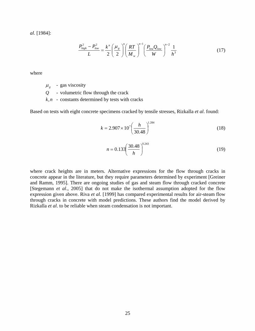
bendn - number of right angle bends in the crack A hydrodynamic instability at the exit of a slot can develop, at least in principle, even with laminar flow. [Thomas and Cornelius, 1982] This instability may be responsible for the observation that aerosol particle deposition begins near the exit plane for flow through a slot whereas in deposition usually begins at the inlet to capillaries. 2.1.4 Concrete Cracks Cracks in concrete are often idealized as slots with rough surfaces. A variety of conventions have been developed to describe the dimensions of cracks in concrete. The convention adopted here is shown schematically in Figure 7. This figure shows a concrete block of width Wo, and thickness Lo with a crack of height h. Whether the crack is oriented horizontally, vertically or at some
24
angle, the minimum crack dimension perpendicular to the direction of overall flow is taken here to be the crack height. There does not appear to be a definitive data base on concrete crack heights3
Figure 8. Concrete cracks
produced by tensile stresses (see .) appear to be well approximated by constant height channels or slots. Cracks produced by a combination of tensile and shear forces may be more complicated. (see Figure 9.) Rizkalla et al. [1983] experimented with cracks 20 to 100 µm in height. Experiments by Stegemann et al. [2005] involve crack heights on the order of 200 µm. Geiner and Ramm [1995] derived a model of leak flow through concrete with crack heights of 200 to 1300 µm. Rizkalla et al. cite work on predicting the spacings of cracks in concrete [Leonhardt, 1977] and the variations in crack heights with crack spacing [Beeby, 1979]. Work to relate cracking to an index of concrete damage is underway [Landis et al., 2007] The actual length of a crack pathway, L, can be longer than the thickness of the concrete structure, Lo. The ratio of these lengths is called the crack tortuosity:
oL
L=τ (16)
Other definitions of tortuosity abound in the literature. Crack tortuosities, as defined here, are thought not to be especially high [Schlangen and Garboczi, 1996]. Gelain and Vendel [2008] found tortuosity of 1.27 for membrane stress cracks through a 10 cm concrete panel and compared this to values of 1.36 and 1.249 reported by others. Boussa et al. [2001] have taken a more detailed examination of cracks in concrete. They note that deviations in the crack pathway occur wherever the crack encounters large aggregate or the like. They conceive of concrete cracks being composed of short straight segments. The ends of the segments are marked by modest changes in direction. Statistical analyses of segments in cracks of various types led these investigators to suggest that angular change in direction (degrees) is normally distributed with mean zero and standard deviation between 20 and 30 degrees. They argue somewhat less persuasively that the lengths of segments are also normally distributed with mean values of 0.54 to 0.71 mm and standard deviations in the range of 0.28 to 0.40 mm. They suggest that the variations in mean and standard deviations of these measures of the segments can be related to concrete manufacture, but do not provide a useful correlation. Meander of the crack as well as intersection with other cracks can make the crack width, W, perpendicular to the overall direction of flow much greater than the width of the concrete panel, Wo. Another type of tortuosity could be defined by the ratio of these two dimensions, though normally this is not done. Though cracks may be approximated as constant height slots, they cannot be considered to have smooth surfaces. This complicates the prediction of flow through concrete cracks. Pan, Marchertas and Kennedy [1984] recommend the isothermal flow equation derived by Rizkalla et
3 In the structural mechanics literature, crack heights are sometimes termed “crack displacements or “crack opening displacements”
25
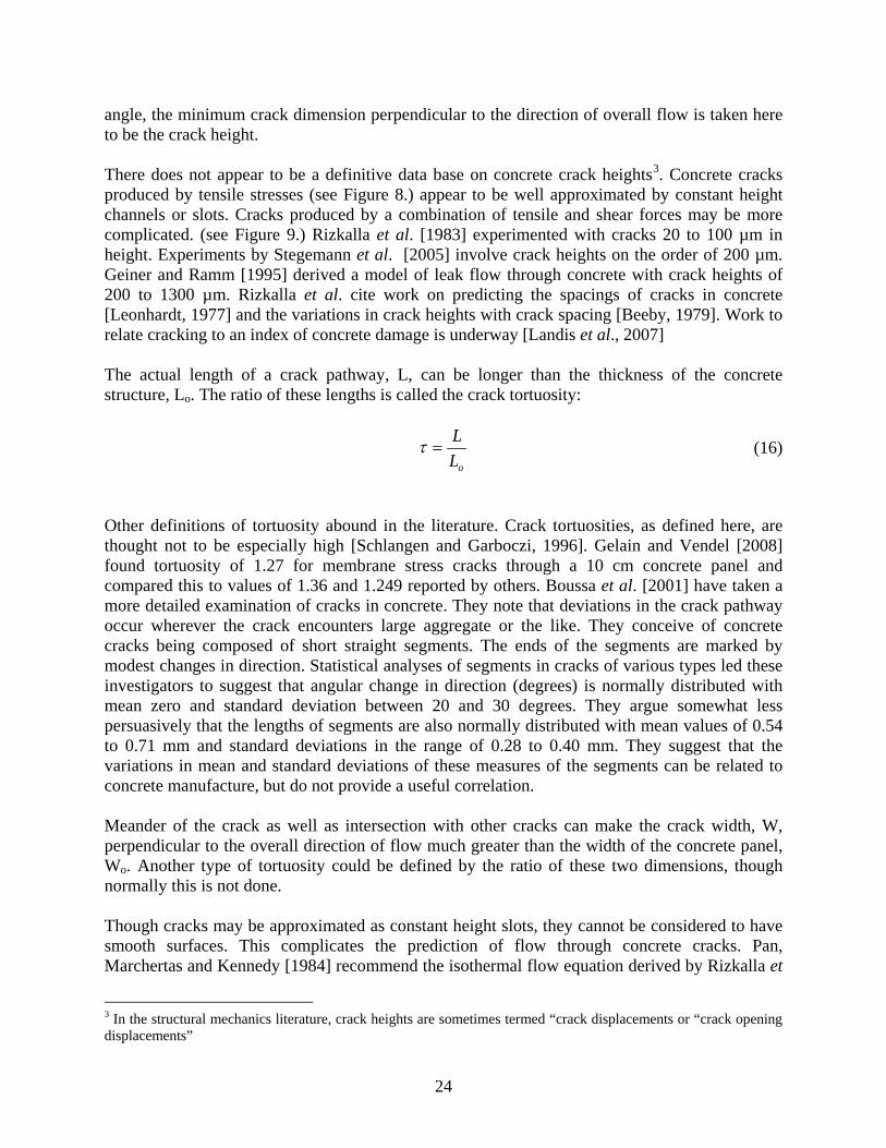
al. [1984]:
3
2122 122 hW
QPMRTk
LPP n
lowlow
n
w
ng
nlowhigh
−−
=
− µ (17)
where
gµ - gas viscosity Q - volumetric flow through the crack
nk, - constants determined by tests with cracks Based on tests with eight concrete specimens cracked by tensile stresses, Rizkalla et al. found:
284.1
7
48.3010907.2
×=
hk (18)
243.048.30133.0
=
hn (19)
where crack heights are in meters. Alternative expressions for the flow through cracks in concrete appear in the literature, but they require parameters determined by experiment [Greiner and Ramm, 1995]. There are ongoing studies of gas and steam flow through cracked concrete [Stegemann et al., 2005] that do not make the isothermal assumption adopted for the flow expression given above. Riva et al. [1999] has compared experimental results for air-steam flow through cracks in concrete with model predictions. These authors find the model derived by Rizkalla et al. to be reliable when steam condensation is not important.
26
Figure 7. Crack Dimensions.

27
Figure 8. Cracks Produced in Concrete by Predominantly Membrane Stress.

28
Figure 9. Concrete Cracks Produced by Membrane and Shear Stress at a Penetration.

29
2.1.5 Gasket Leaks Hirao et al. [1993] characterize the onset pressure and temperature for leaks in hatch flange gaskets. They do not provide data on leak flow, but they do provide qualitative information on leak cross-section. The remarkable findings by Hirao et al. is the time at temperature required for leaks to develop in a pressurized system. This could mean that aerosol available to enter the leak will have aged and be depleted of the larger particle size material before a leak develops.

30
31
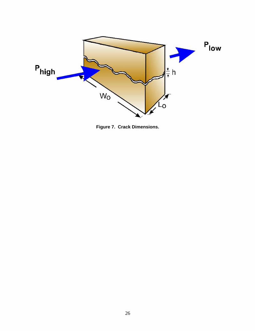
2.2 Individual Experimental Studies Synoptic accounts of individual experimental investigations are provided in the subsections that follow. 2.2.1 Experiments with Capillaries by Mitchell and Coworkers The most comprehensive response to the Morewitz-Vaughan correlation was launched in the United Kingdom in an effort by J.P. Mitchell and coworkers [Burton et al., 1993; Morton and Mitchell, 1995]. The experimental studies involved flow of aerosol through capillaries 19 to 21 mm long with bores of 28 to 35 :m. Most of the experiments used nearly spherical glass spheres as the aerosol. A typical size distribution for the glass sphere is shown in Figure 10. Concentrations of the glass spheres in the source volume leading to the capillary leaks were modest in comparison to concentrations used in many of the experiments used to support the Morewitz-Vaughan correlation. Typically, these concentrations were only 1-3 g/m3
at the start of
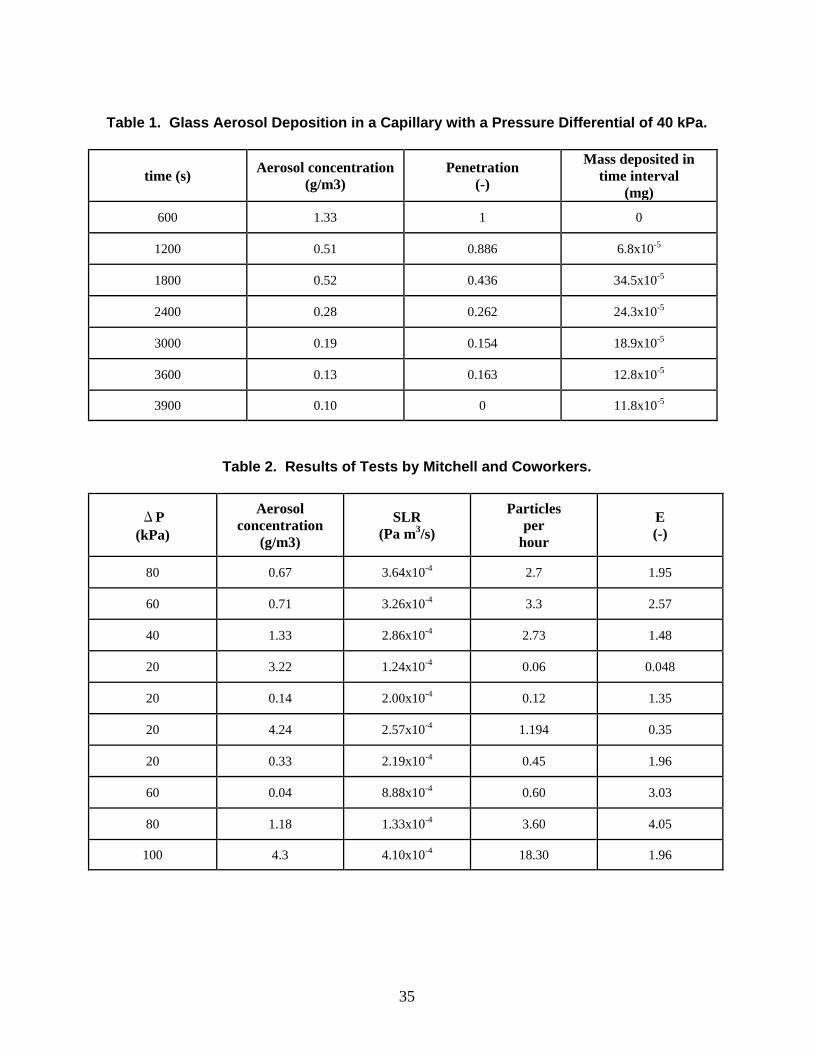
a test and declined due to sedimentation within the source volume as the experiment progressed. Some experiments were done with cerium oxide particles which would have modest deviations from spherical shapes. Pressure differentials used to produce flow through the capillary leak paths were 20, 40, 60, and 80 kPa. Some results of the tests are shown in Figure 11. Results of the test at 40 kPa pressure differential are listed in Table 1. An effectiveness factor termed “penetration” is shown in this table. Penetration is the fraction of the aerosol estimated to enter the capillary (based on gas flow and aerosol concentration) that emerges from the capillary It was found that at 20 kPa, capillaries plugged almost immediately. At a pressure differential of 80 kPa, plugging did not occur over the duration of the experiment though some fluctuations in the volumetric flow rate through the capillaries were observed. At intermediate pressure differentials, there was a slow reduction in the volumetric flow as the capillaries became plugged with aerosol. The initiation of plugging was in the entrance region of the capillaries. In the laminar flow regime of the tests done by Mitchell and coworkers, the dominant deposition mechanisms for aerosol particles are expected to be gravitational settling and diffusion to the walls. Settling and diffusion will lead to deposition if there is sufficient particle residence time in the flow pathway. It would be expected, then, that as flow velocity increases (and residence time decreases) that particle penetration would increase as long as flow remained in the laminar regime. As shown by the plot of penetration against Reynolds number (see Figure 12), this seemed to be the case in the tests done by Mitchell and co-workers. Mitchell and coworkers employ an unusual metric termed the “standardized leak rate” (SLR) to characterize their experimental conditions. The standardized leak rate is related to the velocity of flow through the capillary by:
32
( ) ( )mDDPPSLR
PPPsmv
dus
du
µπ 222
22 29128=
−−
= (20)
where
uP - upstream pressure
dP - downstream pressure
sP - 100 kPa D - capillary inner diameter SLR - standardized leak rate
A leakage “efficiency”, E, is also defined that is better viewed as a figure of merit since the efficiency is not constrained to lie between zero and unity. Some results in terms of these unique quantities are shown in Table 2. The efficiency of aerosol penetration would be expected to depend on aerosol particle size. The distribution of particle sizes that emerge from a capillary should differ, then, from that entering the capillary. A comparison of particle size distributions input and emerging from a 70 µm diameter capillary reported by Mitchell, Edwards and Ball [1990] are shown in Figure 13. Evidently, losses during flow through the capillary are predominantly from the smaller particle size portion of the distribution. This is indicative, of course, of a diffusive particle deposition process. An important result from the test by Mitchell and coworkers is that very frequently capillaries could become plugged with respect to aerosol transport, but gas flow would continue. Some examples are shown for 30 µm capillaries in Table 3. The aerosols used in the tests were, of course, not radioactive. In the case of reactor accidents with radioactive aerosols plugging the pathways, deposits would be heated by decay energy. Continued flow of gas over the deposits raises the possibility that more volatile radionuclide might evaporate from the deposits and be carried through the passage.

33
Figure 10. Size Distribution of Glass Sphere Aerosols Used in Tests by Mitchell and Coworkers.
Figure 11. Flow Through Capillaries Exposed to Glass Sphere Aerosol.

34
Figure 12. Number of Particles that Emerged from Capillaries After 2 Hours.
Figure 13. Comparison of Probability Density Function for the Number Distributions of Aerosol Input and Exiting from a 5 cm long 70 µm Capillary.
35
Table 1. Glass Aerosol Deposition in a Capillary with a Pressure Differential of 40 kPa.
time (s) Aerosol concentration (g/m3)
Penetration (-)
Mass deposited in time interval
(mg) 600 1.33 1 0
1200 0.51 0.886 6.8x10⁻⁵
1800 0.52 0.436 34.5x10⁻⁵
2400 0.28 0.262 24.3x10⁻⁵
3000 0.19 0.154 18.9x10⁻⁵
3600 0.13 0.163 12.8x10⁻⁵
3900 0.10 0 11.8x10⁻⁵
Table 2. Results of Tests by Mitchell and Coworkers.
ΔP (kPa)
Aerosol concentration
(g/m3)
SLR (Pa m3/s)
Particles per
hour
E (-)
80 0.67 3.64x10⁻⁴ 2.7 1.95
60 0.71 3.26x10⁻⁴ 3.3 2.57
40 1.33 2.86x10⁻⁴ 2.73 1.48
20 3.22 1.24x10⁻⁴ 0.06 0.048
20 0.14 2.00x10⁻⁴ 0.12 1.35
20 4.24 2.57x10⁻⁴ 1.194 0.35
20 0.33 2.19x10⁻⁴ 0.45 1.96
60 0.04 8.88x10⁻⁴ 0.60 3.03
80 1.18 1.33x10⁻⁴ 3.60 4.05
100 4.3 4.10x10⁻⁴ 18.30 1.96
36
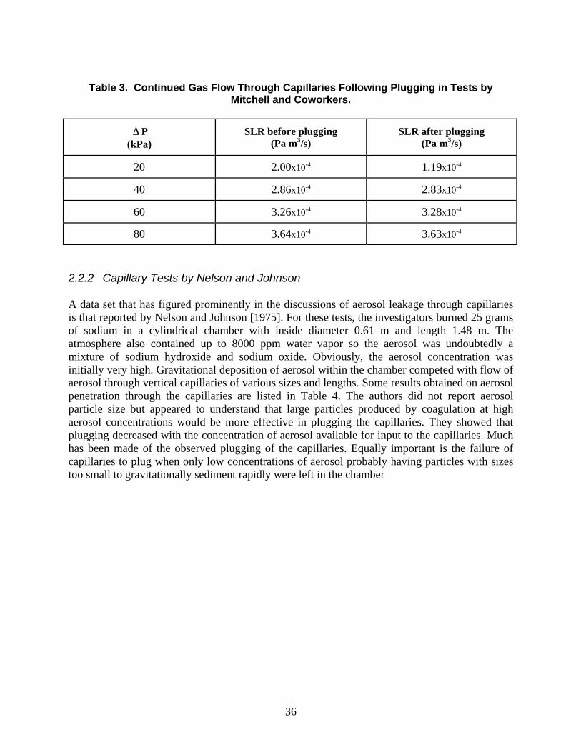
Table 3. Continued Gas Flow Through Capillaries Following Plugging in Tests by
Mitchell and Coworkers.
ΔP (kPa)
SLR before plugging (Pa m3/s)
SLR after plugging (Pa m3/s)
20 2.00x10⁻⁴ 1.19x10⁻⁴
40 2.86x10⁻⁴ 2.83x10⁻⁴
60 3.26x10⁻⁴ 3.28x10⁻⁴
80 3.64x10⁻⁴ 3.63x10⁻⁴ 2.2.2 Capillary Tests by Nelson and Johnson A data set that has figured prominently in the discussions of aerosol leakage through capillaries is that reported by Nelson and Johnson [1975]. For these tests, the investigators burned 25 grams of sodium in a cylindrical chamber with inside diameter 0.61 m and length 1.48 m. The atmosphere also contained up to 8000 ppm water vapor so the aerosol was undoubtedly a mixture of sodium hydroxide and sodium oxide. Obviously, the aerosol concentration was initially very high. Gravitational deposition of aerosol within the chamber competed with flow of aerosol through vertical capillaries of various sizes and lengths. Some results obtained on aerosol penetration through the capillaries are listed in Table 4. The authors did not report aerosol particle size but appeared to understand that large particles produced by coagulation at high aerosol concentrations would be more effective in plugging the capillaries. They showed that plugging decreased with the concentration of aerosol available for input to the capillaries. Much has been made of the observed plugging of the capillaries. Equally important is the failure of capillaries to plug when only low concentrations of aerosol probably having particles with sizes too small to gravitationally sediment rapidly were left in the chamber

37
Table 4. Results From Tests with Sodium Oxide and Sodium Hydroxide Aerosols
Reported by Nelson and Johnson [1975].
Capillary Dimensions Aerosol
Concentration (g/m3)
Gas Flow Prior to Plugging
(dm3)
Entering Aerosol mass prior to
plug (mg)
Time to plug (min) ID
(cm) Length
(cm) 0.052 4.9 15-11 ~0.06 0.65-0.9 0.125 ± 0.025 0.052 4.9 12.5-9.5 0.12 1.4 ± 0.1 2.55 ± 0.35 0.052 4.9 10-7 0.14 1.2 ± 0.2 2.3 ± 0.8 0.052 4.9 4.2-2.8 0.25 0.85 ± 0.15 3.6 ± 0.7 0.052 4.9 1.9-0.047 163 did not plug 0.08 7.6 ~5.8 0.16 ~0.93 ~0.3 0.08 7.6 ~4.4 0.2 ~0.88 1.3 ± 0.2 0.08 7.6 1.5-1.25 1.07 1.5 7.0 ± 0.5 0.08 7.6 0.26-0.17 5.55 1.3 26 ± 5 0.08 7.6 0.13-0.0001 57 did not plug
0.107 3.8 2.1-3 5.5 14.3 0.107 7.6 0.75-1.6 17 19.4 0.107 3.8 0.7-0.4 19.75 9.5 0.107 7.6 20-25 29 did not plug 0.107 7.6 0.14-0.0001 1550 did not plug 0.132 3.8 9.8-9.0 10 92 0.132 7.6 6.2-1.3 30.5 95 0.157 7.6 18-15 3.5 58 0.157 7.6 21-8 68 did not plug
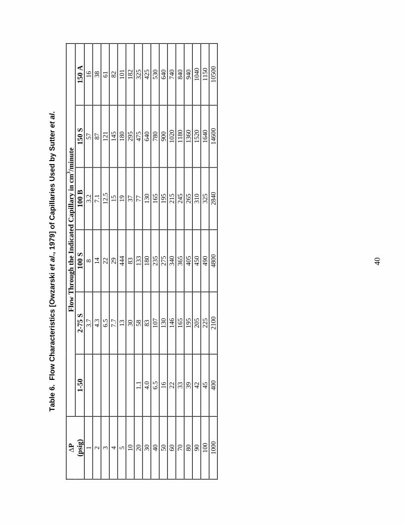
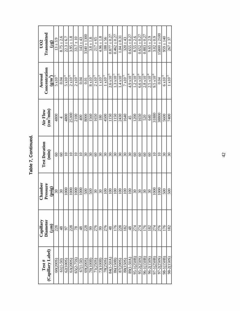
2.2.3 Tests of Depleted Uranium Dioxide Flow Through Capillaries. Sutter et al. [1980] have examined the transport of depleted uranium dioxide powders through capillaries with internal diameters of 48, 78, 114.3, 182, 229, and 275 µm. Characteristics of the capillaries measured by Owzarski et al. [1979] are listed in Table 5. Flows through the capillaries as functions of pressure are provided in Table 6 and shown in Figure 14. The particles in the uranium dioxide powder had mean sizes of 1 µm but were extensively aggregated. The powders were dispersed with a low velocity gas flow through a bed so that concentrations were controlled in the test rather than decaying rapidly due to gravitational settling within the generation volume. No effort was made to characterize the size distribution of the airborne material, but mass concentrations were measured. Aerosol concentration were very much lower than those used in other investigations. Consequently, aerosol growth by coagulation probably does not complicate the interpretation of the results. Tests were done with the leak paths above and below the powder bed. Only tests with leaks above the powder bed are of interest for the purposes of this work. Some of the data reported by Sutter et al. are shown in Table 7. The uranium dioxide that penetrated the capillaries in the tests is plotted in Figure 15 against the mass of uranium expected if there was 100% penetration. The diagonal line in this plot is indicative of perfect agreement between observations and expectations based on 100% penetration.

38
Sutter et al. found two regimes of behavior depending on the dimensional metric Φ: PA ∆=Φ ln (21) where
A - leak area (µm)2 P∆ - pressure difference (psig)
The two regimes are:
• Φ < 10.5
For this regime a maximum of 46 µg of particulate material passed through the leaks.
• Φ > 10.5
Leakage in this regime could be correlated by the expression:
( ) ( )3-N
error std.3lnln 21212−±∆++= − NtPbAbamUO α (22)
where m is the mass of uranium dioxide in µg that leaks and ( )nt 21 α− is the critical value of the Student’s t-statistic for a confidence of 100 (1 -α)% and n degrees of freedom. Parametric values for capillaries are listed in Table 8.

39
Table 5. Characteristics of Capillaries Used by Sutter et al.
Capillary Label Length (cm)
Inside Diameter (µm) Roughness
1-50 2.54 48 0.087 2-75S 0.762 78 0.028 100S 0.762 114.3 0.028 100B 2.85 114.3 0.028 150S 0.767 182 0.014 150A 2.54 189 0.014 150B 2.63 176 0.014 200S 0.759 228 0.0043 200B 2.61 231 0.0043 250S 0.782 276 0.0044 250A 2.62 274 0.0044 250B 2.69 274 0.0011
Figure 14. Flow Characteristics of Capillaries Used by Sutter et al. [Owzarski et al., 1979].
40
Tabl
e 6.
Flo
w C
hara
cter
istic
s [O
wza
rski
et a
l., 1
979]
of C
apill
arie
s U
sed
by S
utte
r et a
l.
ΔP
(psi
g)
Fl
ow T
hrou
gh th
e In
dica
ted
Cap
illar
y in
cm
3 /min
ute
1-50
2-
75 S
10
0 S
10
0 B
15
0 S
15
0 A
1
3.7
8
3.
2
57
16
2
4.
3
14
7.1
87
38
3
6.5
22
12
.5
121
61
4
7.7
29
15
14
5
82
5
13
44
4
19
180
10
1
10
30
83
37
29
5
182
20
1.
1
58
133
77
47
5
325
30
4.
0
83
180
13
0
640
42
5
40
6.5
10
7
235
16
5
780
53
0
50
16
130
27
5
195
90
0
640
60
22
14
6
340
21
5
1020
74
0
70
33
165
36
5
245
11
80
840
80
39
19
5
405
26
5
1360
94
0
90
42
205
45
0
310
15
20
1040
10
0
45
225
49
0
325
16
40
1150
10
00
400
21
00
4800
28
40
1460
0
1050
0

41
Tabl
e 7.
Res
ults
of T
ests
by
Sutte
r et a
l. w
ith C
apill
arie
s
Tes
t #
(Cap
illar
y L
abel
)
Cap
illar
y D
iam
eter
(µ
m)
Cha
mbe
r Pr
essu
re
(psi
g)
Tes
t Dur
atio
n (m
in)
Air
Flo
w
(cm
3 /min
)
Aer
osol
C
once
ntra
tion
(g/m
3 )
UO
2 T
rans
mitt
ed
(µg)
14
(250
A)
274
50
0
30
5400
2x
10-4
30
.4 ±
9.1
15
(150
A)
189
10
00
10
1050
0
0.01
2
1280
± 6
60
26(1
50B
) 17
6
500
30
56
00
4
720
± 33
0
28(2
00B
) 23
1
500
10
20
000
0.
01
2690
± 1
100
34
(250
A)
274
30
30
11
80 (p
lugg
ed)
3x10
-5
2.4
± 1.
6
37(2
50B
) 27
4
30
60
520
2x
10-4
5.
9 ±
1.8
41
(150
S)
182
10
00
10
1460
0
1x10
-3
212
± 64
43
(150
S)
182
50
0
30
5600
2x
10-3
29
0 ±
87
44(1
50B
) 17
6
30
60
520
4x
10-4
12
.4 ±
3.7
45
(150
S)
182
30
60
64
0
5x10
-4
18.0
± 5
.4
50(1
00B
) 99
10
00
10
3140
3x
10-3
87
.8 ±
26
52
(100
B)
99
1000
10
40
0
2x10
-3
6.2
± 1.
9
54(1
00B
) 99
50
0
30
195
0.
0007
4.
07 ±
1.7
55
(250
S)
276
10
00
10
3880
0
0.02
92
10 ±
360
57
(1-5
0)
48
500
30
19
5
4 x1
0-3
25 ±
7.5
58
(250
S)
276
50
0
30
1330
0
2 x1
0-3
675
± 20
0
42
Tabl
e 7,
Con
tinue
d.
Tes
t #
(Cap
illar
y L
abel
)
Cap
illar
y D
iam
eter
(µ
m)
Cha
mbe
r Pr
essu
re
(psi
g)
Tes
t Dur
atio
n (m
in)
Air
Flo
w
(cm
3 /min
)
Aer
osol
C
once
ntra
tion
(g/m
3 )
UO
2 T
rans
mitt
ed
(µg)
60
(200
S)
228
30
60
4800
5
x10-5
13
± 3
.9
61(1
-50)
48
30
60
4
0.04
8.
75 ±
2.6
62
(100
S)
97
1000
10
48
00
5 x1
0-4
22.3
± 6
.7
63(2
00S)
22
8 10
00
10
2530
0 2
x10-5
3.
95 ±
1.8
65
(2-7
5S)
78
1000
10
21
00
2 x1
0-3
33.7
± 1
0 67
(1-5
0)
48
1000
10
40
0 0.
04
143
± 43
69
(200
S)
228
500
30
8000
0.
01
3340
± 1
300
70(1
00B
) 99
50
0 30
15
60
8 x1
0-5
3.8
± 1.
8 71
(250
S)
276
30
60
1650
2
x10-3
21
7 ±
65
73(1
00B
) 99
30
30
18
0 1
x10-3
4.
96 ±
1.8
78
(250
S)
276
100
30
4500
1
x10-3
18
8 ±
56
84(1
-50A
) 48
10
0 30
11
50
2.6
x10-5
0.
877
± 0.
27
86(1
50B
) 17
6 10
0 30
11
50
1.3
x10-5
0.
462
± 0.
27
87(2
00S)
22
8 10
0 30
24
30
1.4
x10-5
1.
04 ±
0.3
1 88
(150
S)
182
100
30
1640
7
x10-3
32
0 ±
43
89(1
-50A
) 48
10
0 30
45
4.
9 x1
0-4
0.65
5 ±
0.27
95
-1(2
50B
) 27
4 30
60
12
00
1.2
x10-4
8.
55 ±
2.6
95
-2(2
50S)
27
4 30
60
16
50
6.6
x10-6
0.
652
± 0.
27
96-1
(150
B)
176
30
60
520
2.8
x10-5
0.
883
± 0.
27
96-2
(150
S)
182
30
60
640
2.5
x10-4
9.
65 ±
2.9
97
-1(2
50B
) 27
4 10
00
10
3188
0 9.
5 x1
0-6
3.02
± 0
.9
97-2
(250
S)
276
1000
10
38
800
0.04
15
800
± 21
00
98-1
(150
B)
176
500
30
5600
6
x10-3
95
9 ±
140
98-2
(150
S)
182
500
30
7400
1
x10-3
26
7 ±
37
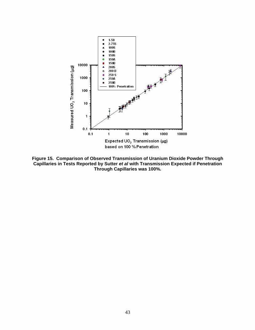
43
Figure 15. Comparison of Observed Transmission of Uranium Dioxide Powder Through Capillaries in Tests Reported by Sutter et al with Transmission Expected if Penetration
Through Capillaries was 100%.

44
Table 8. Parametric Values for Capillaries.
Parameter Capillary
a -17.9875
b1 2.1658
b2 0.1170
N 37
std. error 1.1379
R2 0.6634
45
2.2.4 Rockwell Tests on Capillary Flow Rockwell International [1977] reported results of aerosol plugging capillaries as a function of capillary diameter, capillary length and pressure differential. These results, extracted from graphs, are shown in Table 9. Aerosols were sodium oxide and sodium carbonate. Particle size information was not given, but in light of the rather high concentrations, it would be expected that particles would be rather large (~10 µm). Without particle size information there is rather little that can be done with these data aside from developing correlations of the type proposed by Morewitz and Vaughan. An interesting feature of the tests is the observation that plugging differed in capillaries with sharp opening than in capillaries with rounded openings.
46
Table 9. Capillary Plugging Results Reported by Rockwell International [1997].
ΔP (kPa)
Capillary diameter
(cm)
Capillary Length (cm)
Aerosol Concentration
(g/m3)
mass passing through prior to
plugging (mg)
3.45 0.108 3.8 14-16.5 1.4
6.93 0.108 3.8 14-16.5 6.9
12.5 0.108 3.8 14-16.5 15
13.6 0.108 3.8 14-16.5 49
27.2 0.108 3.8 14-16.5 107
3.45 0.132 5.1 6-10.5 0.25
3.45 0.132 15.2 6-10.5 0.49
3.45 0.132 10.1 6-10.5 1.5
3.45 0.132 20.4 6-10.5 2.4
3.45 0.132 17.9 6-10.5 3.9
2.9 to 6.9 0.041 5.0 1.3-1.7 13
2.9 to 6.9 0.059 5.0 1.3-1.7 15
2.9 to 6.9 0.059 5.0 1.3-1.7 23
2.9 to 6.9 0.108 5.0 1.3-1.7 70
2.9 to 6.9 0.108 5.0 1.3-1.7 70
2.9 to 6.9 0.108 5.0 1.3-1.7 83
47
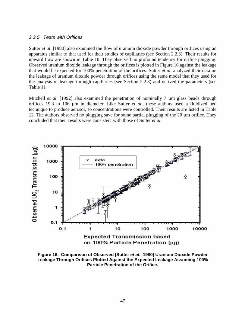
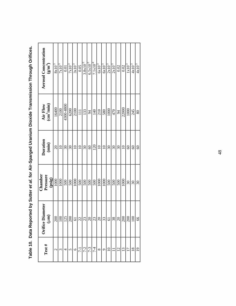
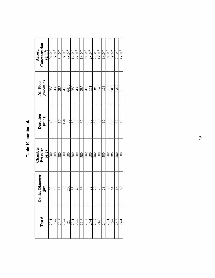
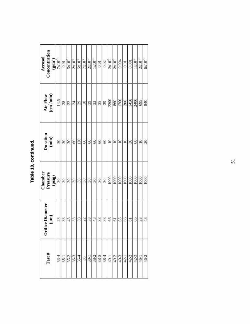
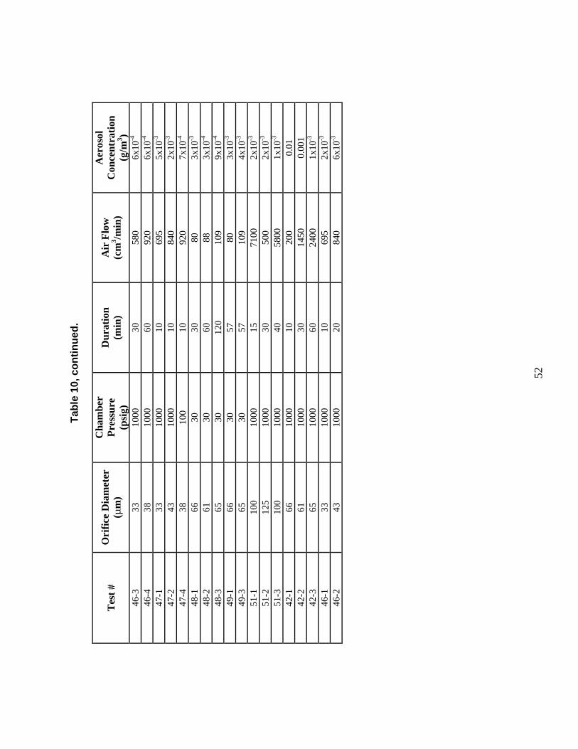
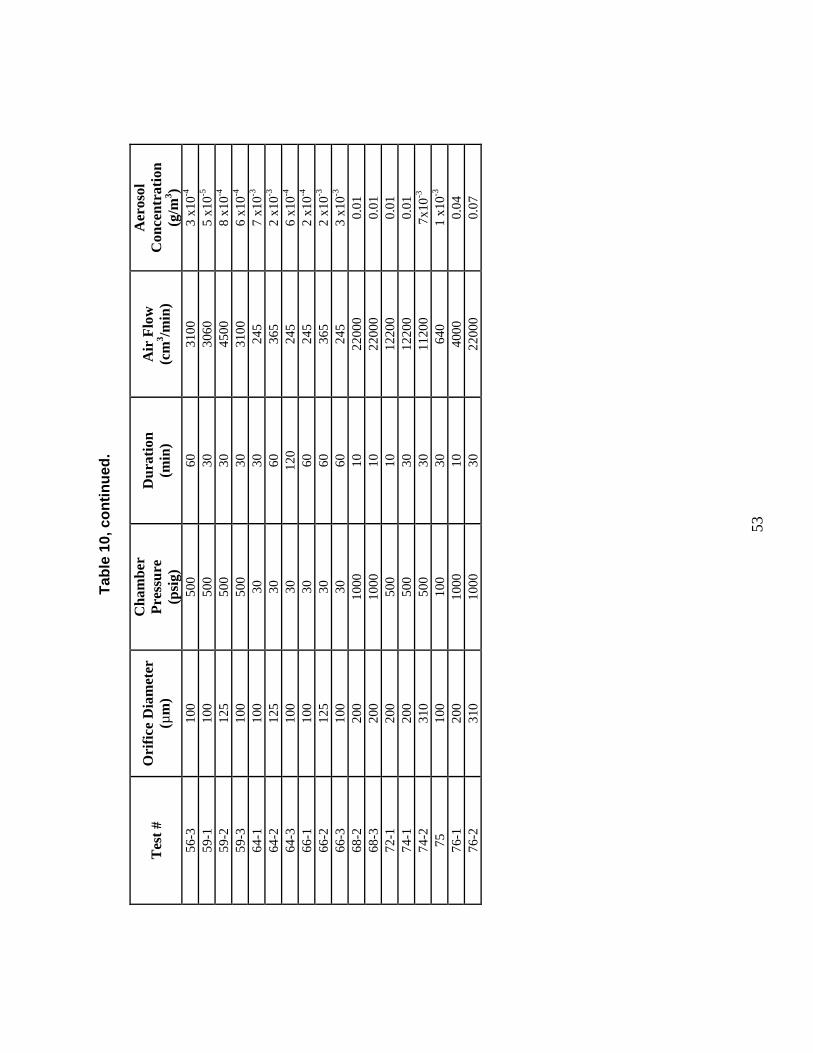
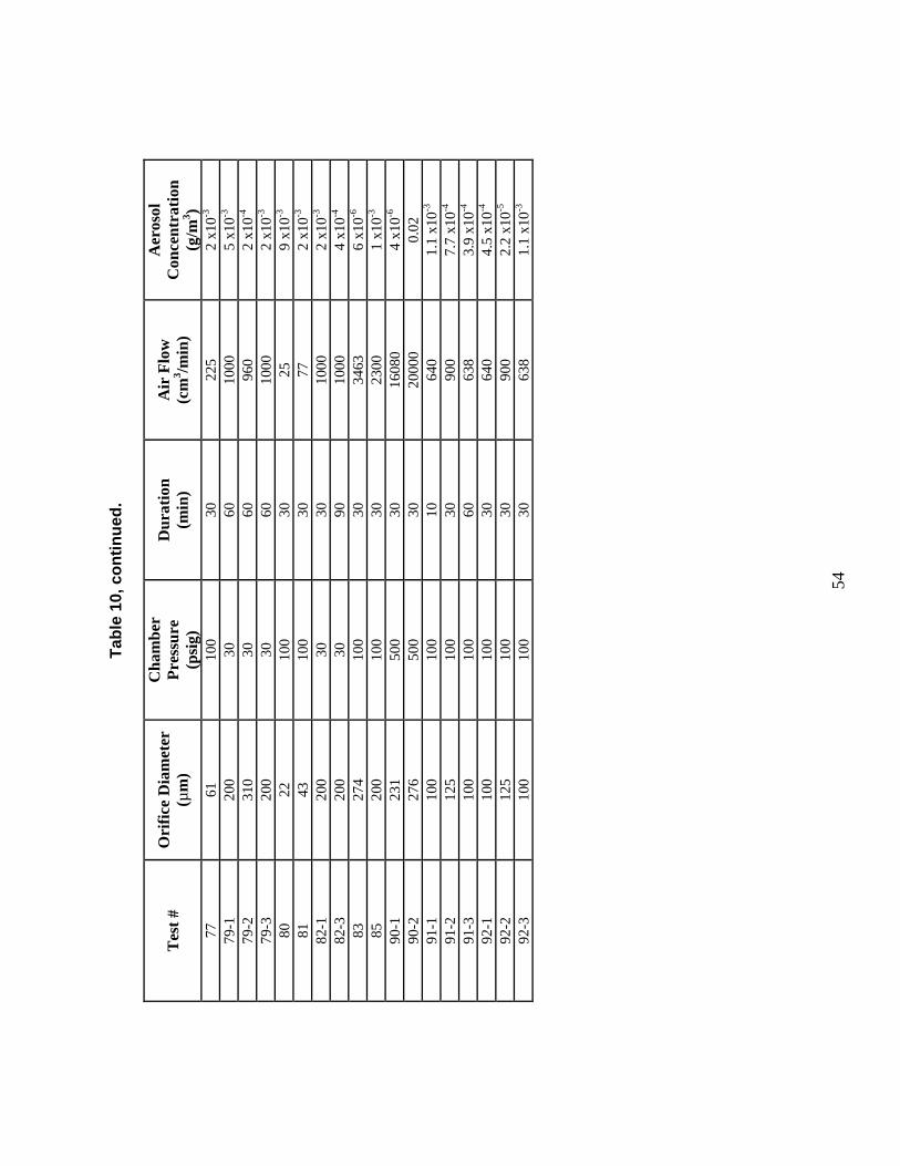
2.2.5 Tests with Orifices Sutter et al. [1980] also examined the flow of uranium dioxide powder through orifices using an apparatus similar to that used for their studies of capillaries (see Section 2.2.3). Their results for upward flow are shown in Table 10. They observed no profound tendency for orifice plugging. Observed uranium dioxide leakage through the orifices is plotted in Figure 16 against the leakage that would be expected for 100% penetration of the orifices. Sutter et al. analyzed their data on the leakage of uranium dioxide powder through orifices using the same model that they used for the analysis of leakage through capillaries (see Section 2.2.3) and derived the parameters (see Table 11 Mitchell et al. [1992] also examined the penetration of nominally 7 µm glass beads through orifices 19.3 to 106 µm in diameter. Like Sutter et al., these authors used a fluidized bed technique to produce aerosol, so concentrations were controlled. Their results are listed in Table 12. The authors observed no plugging save for some partial plugging of the 20 µm orifice. They concluded that their results were consistent with those of Sutter et al.
Figure 16. Comparison of Observed [Sutter et al., 1980] Uranium Dioxide Powder Leakage Through Orifices Plotted Against the Expected Leakage Assuming 100%
Particle Penetration of the Orifice.
48
Tabl
e 10
. D
ata
Rep
orte
d by
Sut
ter e
t al.
for A
ir-Sp
arge
d U
rani
um D
ioxi
de T
rans
mis
sion
Thr
ough
Orif
ices
.
Tes
t #
Ori
fice
Dia
met
er
(µm
)
Cha
mbe
r Pr
essu
re
(psi
g)
Dur
atio
n (m
in)
Air
Flo
w
(cm
3 /min
) A
eros
ol C
once
ntra
tion
(g/m
3 )
2
200
10
00
20
1640
0
8x10
-3
3
100
10
00
10
2100
7x
10-3
4
12
5
500
30
43
00-4
800
0.
01
5
200
50
0
30
6200
7x
10-3
6
61
10
00
10
2100
3x
10-3
7-
1
22
500
10
11
1
0.05
7-
2
23
500
30
13
3
3.8x
10-3
7-
3
20
500
60
94
6.
5x10
-3
7-4
23
50
0
120
14
0
7.1x
10-4
8
20
10
00
10
210
6x
10-3
9
33
10
00
10
580
6x
10-3
10
61
50
0
30
1000
2x
10-3
11
38
50
0
30
470
2x
10-3
12
20
50
0
30
94
0.02
13
20
0
1000
10
22
000
0.
02
17
200
30
60
10
00
1x10
-3
18
100
30
60
24
5
4x10
-3
19
66
30
60
80
4x10
-3
49
Tabl
e 10
, con
tinue
d.
Tes
t #
Ori
fice
Dia
met
er
(µm
)
Cha
mbe
r Pr
essu
re
(psi
g)
Dur
atio
n (m
in)
Air
Flo
w
(cm
3 /min
)
Aer
osol
C
once
ntra
tion
(g/m
3 ) 20
-1
33
500
10
35
0
5x10
-3
20-2
43
50
0
30
435
3x
10-3
20
-3
33
500
60
28
5
6x10
-4
20-4
38
50
0
120
47
0
3x10
-4
21
200
50
0
30
6400
7x
10-5
22
-1
33
500
30
35
0
1x10
-3
22-2
43
50
0
30
435
2x
10-3
22
-3
33
500
30
28
5
1x10
-3
22-4
38
50
0
30
470
9x
10-4
24
-1
22
500
30
11
1
2x10
-3
24-2
20
50
0
30
94
2x10
-3
24-3
23
50
0
30
140
1x
10-3
24
-4
23
500
30
13
3
3x10
-3
25-1
66
50
0
30
1100
2x
10-3
25
-2
61
500
30
10
00
3x10
-3
25-3
65
50
0
30
1200
2x
10-3
27
-1
66
500
10
11
00
4x10
-4

50
Tabl
e 10
, con
tinue
d.
Tes
t #
Ori
fice
Dia
met
er
(µm
)
Cha
mbe
r Pr
essu
re
(psi
g)
Dur
atio
n (m
in)
Air
Flo
w
(cm
3 /min
)
Aer
osol
C
once
ntra
tion
(g/m
3 ) 27
-2
61
500
30
10
00
2x10
-4
27-3
65
50
0
60
1200
2x
10-4
29
-1
22
1000
10
27
5
0.01
29
-2
23
1000
10
27
5
3x10
-3
29-3
20
10
00
10
210
0.
01
29-4
23
10
00
10
290
2x
10-3
30
-1
22
1000
10
27
5
3x10
-3
30-2
23
10
00
20
275
7x
10-4
30
-3
20
1000
30
21
0
2x10
-3
30-4
23
10
00
60
290
3x
10-4
31
-1
22
30
10
10
0.07
31
-2
23
30
30
10.3
0.
03
31-3
20
30
60
9.
5
0.02
31
-4
23
30
120
14
.5
6x10
-3
32
43
30
60
20
0.01
33
-1
22
30
30
10
<3x1
0-3
33-2
23
30
30
10
.3
4x10
-3
33-3
20
30
30
9.
5
<3x1
0-3
51
Tabl
e 10
, con
tinue
d.
Tes
t #
Ori
fice
Dia
met
er
(µm
)
Cha
mbe
r Pr
essu
re
(psi
g)
Dur
atio
n (m
in)
Air
Flo
w
(cm
3 /min
)
Aer
osol
C
once
ntra
tion
(g/m
3 ) 33
-4
23
30
30
14.5
7x
10-3
35
-1
33
30
30
28
0.01
35
-2
43
30
30
22
5x10
-3
35-3
33
30
60
24
2x
10-3
35
-4
38
30
120
39
5x
10-3
36
22
30
60
10
7x
10-3
38
-1
33
30
60
39
2x10
-3
38-2
43
30
60
33
1x
10-3
38
-3
33
30
60
35
0.01
38
-4
38
30
60
39
0.02
40
-1
66
1000
10
23
00
2x10
-3
40-2
61
10
00
10
860
2x
10-3
40
-3
65
1000
10
17
60
0.00
4
42-1
66
10
00
10
200
0.
01
42-2
61
10
00
30
1450
0.
001
42
-3
65
1000
60
24
00
1x10
-3
46-1
33
10
00
10
695
2x
10-3
46
-2
43
1000
20
84
0
6x10
-3
52
Tabl
e 10
, con
tinue
d.
Tes
t #
Ori
fice
Dia
met
er
(µm
)
Cha
mbe
r Pr
essu
re
(psi
g)
Dur
atio
n (m
in)
Air
Flo
w
(cm
3 /min
)
Aer
osol
C
once
ntra
tion
(g/m
3 ) 46
-3
33
1000
30
58
0
6x10
-4
46-4
38
10
00
60
920
6x
10-4
47
-1
33
1000
10
69
5
5x10
-3
47-2
43
10
00
10
840
2x
10-3
47
-4
38
100
10
92
0
7x10
-4
48-1
66
30
30
80
3x
10-3
48
-2
61
30
60
88
3x10
-4
48-3
65
30
12
0
109
9x
10-4
49
-1
66
30
57
80
3x10
-3
49-3
65
30
57
10
9
4x10
-3
51-1
10
0
1000
15
71
00
2x10
-3
51-2
12
5
1000
30
50
0
2x10
-3
51-3
10
0
1000
40
58
00
1x10
-3
42-1
66
10
00
10
200
0.
01
42-2
61
10
00
30
1450
0.
001
42
-3
65
1000
60
24
00
1x10
-3
46-1
33
10
00
10
695
2x
10-3
46
-2
43
1000
20
84
0
6x10
-3
53
Tabl
e 10
, con
tinue
d.
Tes
t #
Ori
fice
Dia
met
er
(µm
)
Cha
mbe
r Pr
essu
re
(psi
g)
Dur
atio
n (m
in)
Air
Flo
w
(cm
3 /min
)
Aer
osol
C
once
ntra
tion
(g/m
3 ) 56
-3
100
50
0
60
3100
3
x10-4
59
-1
100
50
0
30
3060
5
x10-5
59
-2
125
50
0
30
4500
8
x10-4
59
-3
100
50
0
30
3100
6
x10-4
64
-1
100
30
30
24
5
7 x1
0-3
64-2
12
5
30
60
365
2
x10-3
64
-3
100
30
12
0
245
6
x10-4
66
-1
100
30
60
24
5
2 x1
0-4
66-2
12
5
30
60
365
2
x10-3
66
-3
100
30
60
24
5
3 x1
0-3
68-2
20
0
1000
10
22
000
0.
01
68-3
20
0
1000
10
22
000
0.
01
72-1
20
0
500
10
12
200
0.
01
74-1
20
0
500
30
12
200
0.
01
74-2
31
0
500
30
11
200
7x
10-3
75
10
0
100
30
64
0
1 x1
0-3
76-1
20
0
1000
10
40
00
0.04
76
-2
310
10
00
30
2200
0
0.07
54
Tabl
e 10
, con
tinue
d.
Tes
t #
Ori
fice
Dia
met
er
(µm
)
Cha
mbe
r Pr
essu
re
(psi
g)
Dur
atio
n (m
in)
Air
Flo
w
(cm
3 /min
)
Aer
osol
C
once
ntra
tion
(g/m
3 ) 77
61
10
0
30
225
2
x10-3
79
-1
200
30
60
10
00
5 x1
0-3
79-2
31
0
30
60
960
2
x10-4
79
-3
200
30
60
10
00
2 x1
0-3
80
22
100
30
25
9
x10-3
81
43
10
0
30
77
2 x1
0-3
82-1
20
0
30
30
1000
2
x10-3
82
-3
200
30
90
10
00
4 x1
0-4
83
274
10
0
30
3463
6
x10-6
85
20
0
100
30
23
00
1 x1
0-3
90-1
23
1
500
30
16
080
4
x10-6
90
-2
276
50
0
30
2000
0
0.02
91
-1
100
10
0
10
640
1.
1 x1
0-3
91-2
12
5
100
30
90
0
7.7
x10-4
91
-3
100
10
0
60
638
3.
9 x1
0-4
92-1
10
0
100
30
64
0
4.5
x10-4
92
-2
125
10
0
30
900
2.
2 x1
0-5
92-3
10
0
100
30
63
8
1.1
x10-3

55
Tabl
e 10
, con
tinue
d.
Tes
t #
Ori
fice
Dia
met
er
(µm
)
Cha
mbe
r Pr
essu
re
(psi
g)
Dur
atio
n (m
in)
Air
Flo
w
(cm
3 /min
)
Aer
osol
C
once
ntra
tion
(g/m
3 ) 93
-1
66
100
10
25
5
3 x1
0-4
93-2
61
10
0
30
225
1
x10-4
93
-3
65
100
60
26
5
1 x1
0-4
94-1
66
10
0
30
255
1.
3 x1
0-4
94-2
61
10
0
30
225
5.
3 x1
0-4
94-3
65
10
0
30
255
3.
0 x1
0-4
96-3
20
0
30
60
1000
2.
8 x1
0-4
98-3
20
0
500
30
11
000
3
x10-3
10
1-1
22
10
0
30
25
0.01
10
1-2
23
10
0
30
29
3.5
x10-3
10
1-3
20
10
0
30
22
2.2
x10-3
10
1-4
23
10
0
30
32
2.5
x10-3
10
3-1
22
10
0
10
25
0.01
3
103-
2
23
100
30
29
3.
8 x1
0-3
103-
3
20
100
60
22
9.
5 x1
0-4
10
3-4
23
10
0
120
32
4
x10-4
10
4-1
20
0
1000
10
18
800
0.
03
104-
2
200
10
00
10
2230
0
8 x1
0-3
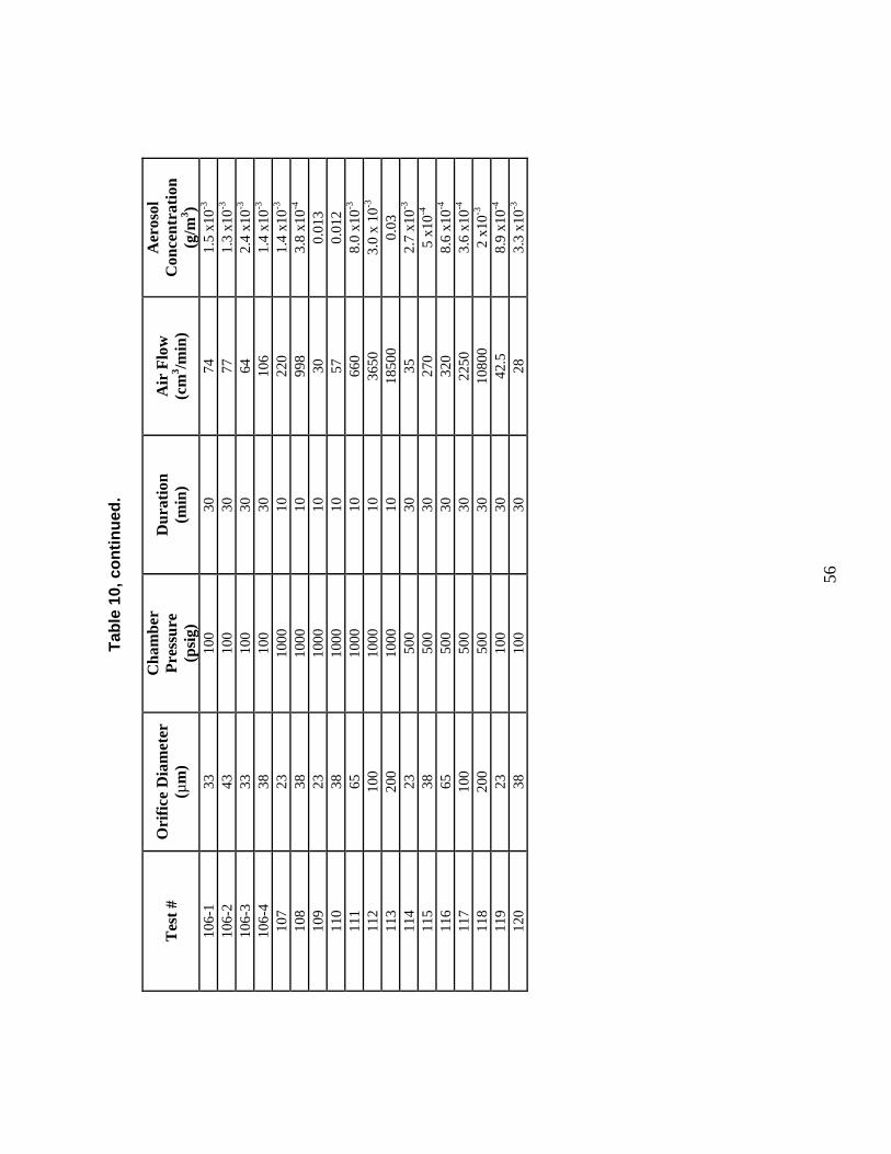
56
Tabl
e 10
, con
tinue
d.
Tes
t #
Ori
fice
Dia
met
er
(µm
)
Cha
mbe
r Pr
essu
re
(psi
g)
Dur
atio
n (m
in)
Air
Flo
w
(cm
3 /min
)
Aer
osol
C
once
ntra
tion
(g/m
3 ) 10
6-1
33
10
0
30
74
1.5
x10-3
10
6-2
43
10
0
30
77
1.3
x10-3
10
6-3
33
10
0
30
64
2.4
x10-3
10
6-4
38
10
0
30
106
1.
4 x1
0-3
107
23
10
00
10
220
1.
4 x1
0-3
108
38
10
00
10
998
3.
8 x1
0-4
109
23
10
00
10
30
0.01
3
110
38
10
00
10
57
0.01
2
111
65
10
00
10
660
8.
0 x1
0-3
112
10
0
1000
10
36
50
3.0
x 10
-3
113
20
0
1000
10
18
500
0.
03
114
23
50
0
30
35
2.7
x10-3
11
5
38
500
30
27
0
5 x1
0-4
116
65
50
0
30
320
8.
6 x1
0-4
117
10
0
500
30
22
50
3.6
x10-4
11
8
200
50
0
30
1080
0
2 x1
0-3
119
23
10
0
30
42.5
8.
9 x1
0-4
120
38
10
0
30
28
3.3
x10-3
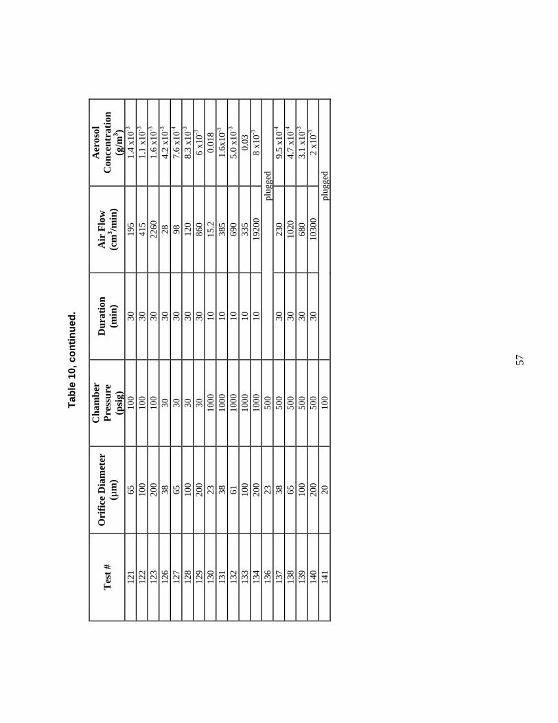
57
Tabl
e 10
, con
tinue
d.
Tes
t #
Ori
fice
Dia
met
er
(µm
)
Cha
mbe
r Pr
essu
re
(psi
g)
Dur
atio
n (m
in)
Air
Flo
w
(cm
3 /min
)
Aer
osol
C
once
ntra
tion
(g/m
3 ) 12
1
65
100
30
19
5
1.4
x10-3
12
2
100
10
0
30
415
1.
1 x1
0-3
123
20
0
100
30
22
60
1.6
x10-3
12
6
38
30
30
28
4.2
x10-3
12
7
65
30
30
98
7.6
x10-4
12
8
100
30
30
12
0
8.3
x10-3
12
9
200
30
30
86
0
6 x1
0-3
130
23
10
00
10
15.2
0.
018
13
1
38
1000
10
38
5
1.6x
10-3
13
2
61
1000
10
69
0
5.0
x10-3
13
3
100
10
00
10
335
0.
03
134
20
0
1000
10
19
200
8
x10-3
13
6
23
500
plug
ged
13
7
38
500
30
23
0
9.5
x10-4
13
8
65
500
30
10
20
4.7
x10-4
13
9
100
50
0
30
680
3.
1 x1
0-3
140
20
0
500
30
10
300
2
x10-3
14
1
20
100
plug
ged
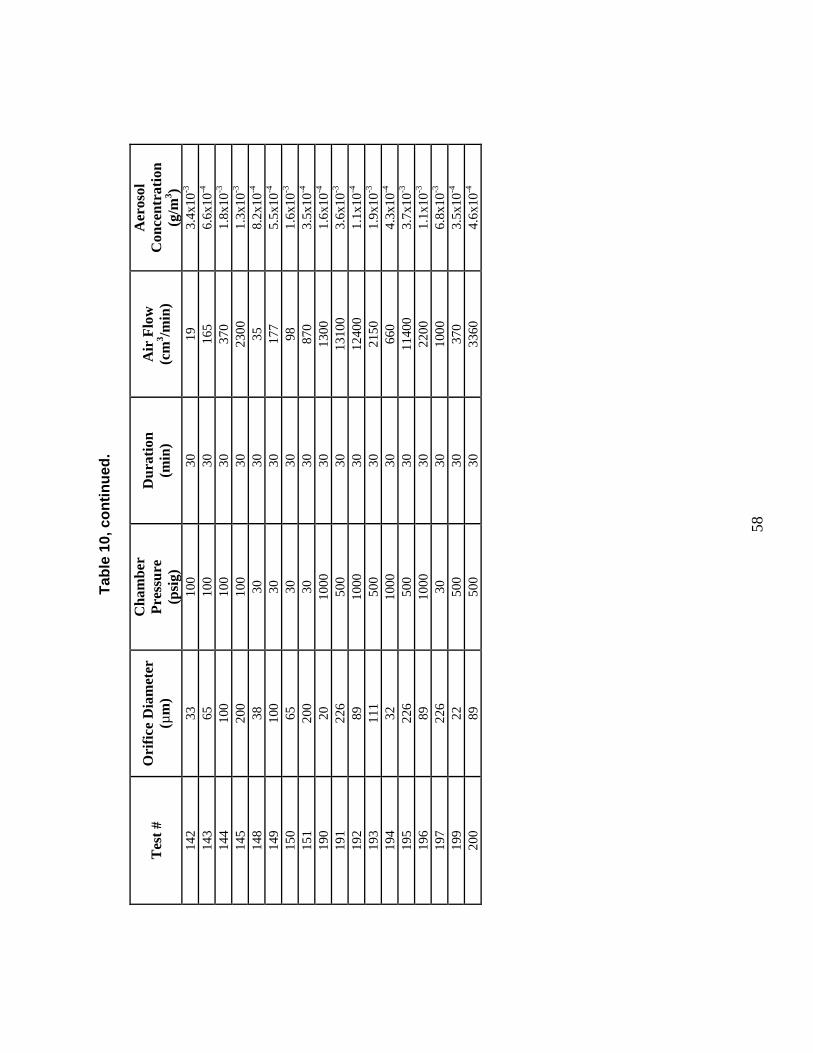
58
Tabl
e 10
, con
tinue
d.
Tes
t #
Ori
fice
Dia
met
er
(µm
)
Cha
mbe
r Pr
essu
re
(psi
g)
Dur
atio
n (m
in)
Air
Flo
w
(cm
3 /min
)
Aer
osol
C
once
ntra
tion
(g/m
3 ) 14
2
33
100
30
19
3.
4x10
-3
143
65
10
0
30
165
6.
6x10
-4
144
10
0
100
30
37
0
1.8x
10-3
14
5
200
10
0
30
2300
1.
3x10
-3
148
38
30
30
35
8.
2x10
-4
149
10
0
30
30
177
5.
5x10
-4
150
65
30
30
98
1.
6x10
-3
151
20
0
30
30
870
3.
5x10
-4
190
20
10
00
30
1300
1.
6x10
-4
191
22
6
500
30
13
100
3.
6x10
-3
192
89
10
00
30
1240
0
1.1x
10-4
19
3
111
50
0
30
2150
1.
9x10
-3
194
32
10
00
30
660
4.
3x10
-4
195
22
6
500
30
11
400
3.
7x10
-3
196
89
10
00
30
2200
1.
1x10
-3
197
22
6
30
30
1000
6.
8x10
-3
199
22
50
0
30
370
3.
5x10
-4
200
89
50
0
30
3360
4.
6x10
-4
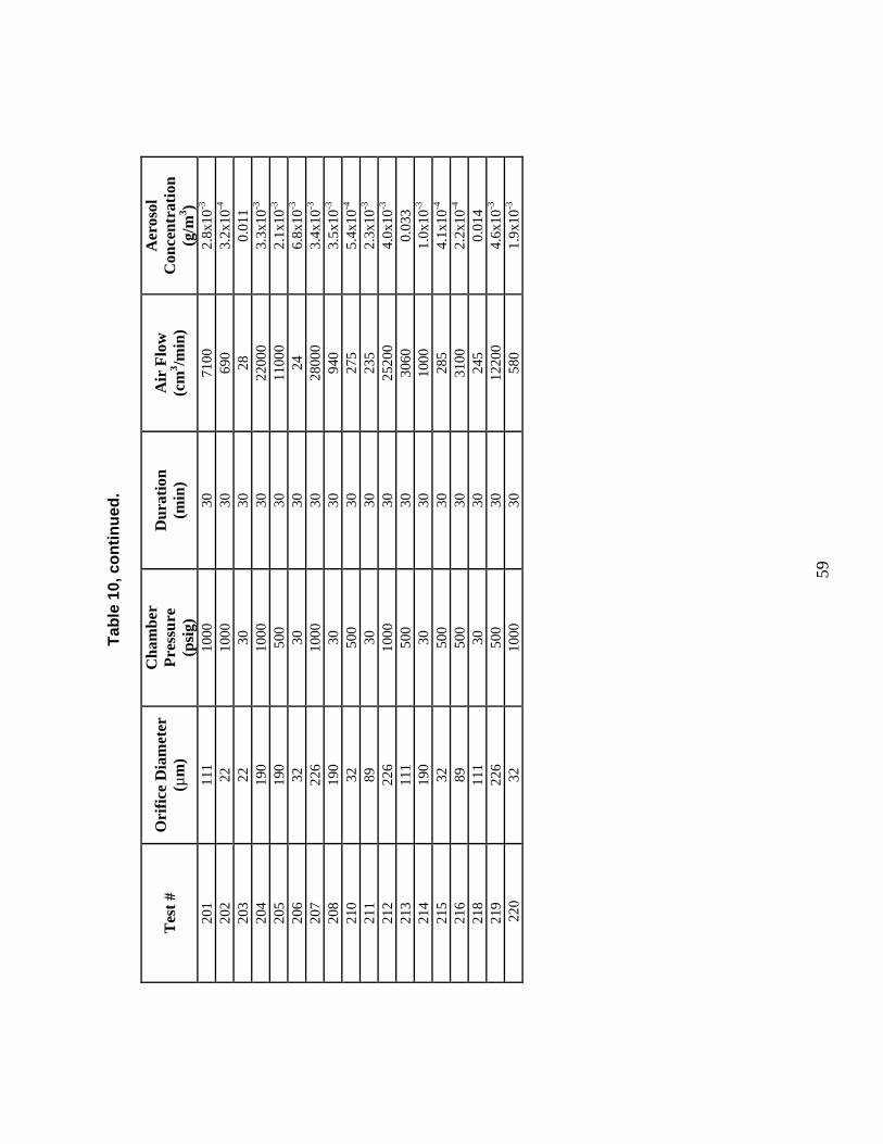
59
Tabl
e 10
, con
tinue
d.
Tes
t #
Ori
fice
Dia
met
er
(µm
)
Cha
mbe
r Pr
essu
re
(psi
g)
Dur
atio
n (m
in)
Air
Flo
w
(cm
3 /min
)
Aer
osol
C
once
ntra
tion
(g/m
3 ) 20
1
111
10
00
30
7100
2.
8x10
-3
202
22
10
00
30
690
3.
2x10
-4
203
22
30
30
28
0.
011
20
4
190
10
00
30
2200
0
3.3x
10-3
20
5
190
50
0
30
1100
0
2.1x
10-3
20
6
32
30
30
24
6.8x
10-3
20
7
226
10
00
30
2800
0
3.4x
10-3
20
8
190
30
30
94
0
3.5x
10-3
21
0
32
500
30
27
5
5.4x
10-4
21
1
89
30
30
235
2.
3x10
-3
212
22
6
1000
30
25
200
4.
0x10
-3
213
11
1
500
30
30
60
0.03
3
214
19
0
30
30
1000
1.
0x10
-3
215
32
50
0
30
285
4.
1x10
-4
216
89
50
0
30
3100
2.
2x10
-4
218
11
1
30
30
245
0.
014
21
9
226
50
0
30
1220
0
4.6x
10-3
2
20
32
1000
30
58
0
1.9x
10-3
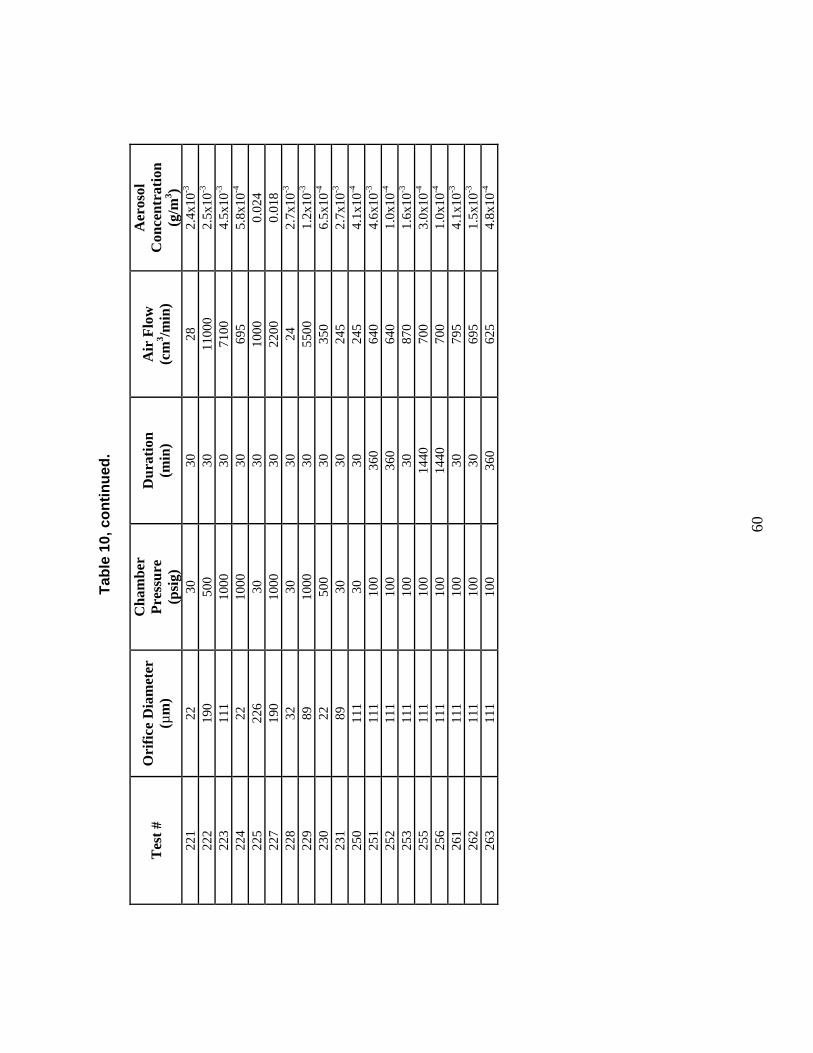
60
Tabl
e 10
, con
tinue
d.
Tes
t #
Ori
fice
Dia
met
er
(µm
)
Cha
mbe
r Pr
essu
re
(psi
g)
Dur
atio
n (m
in)
Air
Flo
w
(cm
3 /min
)
Aer
osol
C
once
ntra
tion
(g/m
3 ) 22
1
22
30
30
28
2.4x
10-3
22
2
190
50
0
30
1100
0
2.5x
10-3
22
3
111
10
00
30
7100
4.
5x10
-3
224
22
10
00
30
695
5.
8x10
-4
225
22
6
30
30
1000
0.
024
22
7
190
10
00
30
2200
0.
018
22
8
32
30
30
24
2.7x
10-3
22
9
89
1000
30
55
00
1.2x
10-3
23
0
22
500
30
35
0
6.5x
10-4
23
1
89
30
30
245
2.
7x10
-3
250
11
1
30
30
245
4.
1x10
-4
251
11
1
100
36
0
640
4.
6x10
-3
252
11
1
100
36
0
640
1.
0x10
-4
253
11
1
100
30
87
0
1.6x
10-3
25
5
111
10
0
1440
70
0
3.0x
10-4
25
6
111
10
0
1440
70
0
1.0x
10-4
26
1
111
10
0
30
795
4.
1x10
-3
262
11
1
100
30
69
5
1.5x
10-3
26
3
111
10
0
360
62
5
4.8x
10-4

61
Table 11. Parametric Values for Orifices.
Parameter Capillary
a -14.1959
b1 1.7906
b2 0.1095
N 91
std. error 0.8718
R2 0.8262
Table 12. Some Results of Experiments by Mitchell et al. [1992] on the Penetration of Orifices by Nominally 7 µm glass Aerosol Particles.
orifice Aerosol
Concentration (Particles/m3)
Leak Rate (particles per
hour) Bore (µm)
Length (µm)
Discharge Coefficient
106 102 0.47 482x106 2.05x10⁶ 41.8 102 0.35 291x106 1.30x10⁶ 37.6 102 0.46 69x106 0.966x10⁶ 32.2 102 0.43 214x106 0.625x10⁶ 20.5 229 0.47 26x106 0.233x10⁶ 20.5 102 0.39 29x106 0.090x10⁶ 19.3 50.9 0.45 62x106 0.0745x10⁶ 20.0 25.4 0.47 43x106 0.0123x10⁶ 21.3 12.7 0.51 281x106 0.227x10⁶ 21.2 509 0.54 88x106 0.349x10⁶

62
2.2.6 Lewis Tests of Particle Transport Through a Slot Lewis [1995] obtained penetration data for various sizes of particles passing through a slot. Particles included talc, fumed silica, precipitated silica, aluminum oxide, titanium dioxide, and Arizona road dust. The slot was 0.1 mm high and 40 mm long. The differential pressure in the tests was 10 kPa. Penetration data were fit to a quadratic polynomial in particle size. What Lewis termed “best fit” results from a variety of tests are shown in Table 13. Results from tests with talc are shown in Table 14. These results are plotted in Figure 17. The size-dependent data are particularly useful for code validation.
Figure 17. Lewis [1995] results for aerosol flow through a 0.1 mm slot at a pressure differential of 10 kPa.

63
Table 13. Results of Lewis’ Test [1995] of Particle Transport Through a Slot (Best Fit
Results).
dp (µm)
Penetration (-)
dp (µm)
Penetration (-)
1.0 0.985 3.46 0.621
1.0 0.935 4.0 0.554
1.5 0.918 4.0 0.521
1.5 0.9 4.5 0.442
2.0 0.86 4.5 0.412
2.0 0.859 5.0 0.315
2.48 0.797 5.0 0.297
2.48 0.794 5.5 0.175
3.0 0.730 5.5 0.173
3.0 0.715 6.0 0.053
3.46 0.647 6.0 0.029
Table 14. Results of Lewis’ Test [1995] of Particle Transport Through a Slot (Data for Talc Particles).
dp
(µm) Penetration
(-) dp
(µm) Penetration
(-)
1.0 0.481 2.29 0.600
1.10 0.842 2.68 0.695
1.20 0.642 3.09 0.543
1.31 0.974 3.46 0.636
1.50 0.736 4.34 0.499
1.60 0.751 4.64 0.284
1.70 0.811 5.89 0.330
1.90 0.478 6.29 0.001

64
2.2.7 Mosley et al. Tests of Aerosol Transport Through a Slot Mosley et al. [2001] reported on the transport of aerosol having aerodynamic mean diameters of 0.05 to 5 µm through a horizontal slot 0.508 mm high, 433 mm wide and 102 mm deep. The slot was made with aluminum sides so surface roughness was quite small. Data were collected with an aerodynamic particle sizer (APS) and an electrical low pressure impactor (ELPI). Some results are shown in Figure 18 through Figure 21. Penetration increases with increasing differential pressure over the range of 2 to 20 kPa. Model predictions shown in the figures were based on considering only diffusion and gravitational sedimentation. The efficiencies of these deposition processes were taken to be additive, so: diffgravoverall PPP = (23) where
overallP - overall penetration of the slot
gravP - penetration if only gravitational sedimentation
= hV
LVsettling
21−
diffP - penetration if only diffusion
=
Vh
Lp2
967.1exp
η
h - crack height The agreement between experimental results and predictions of the simple model is quite noteworthy. Particle sizes examined and hydrodynamic conditions span sufficient range to test well diffusion and gravitational settling models for laminar flow.
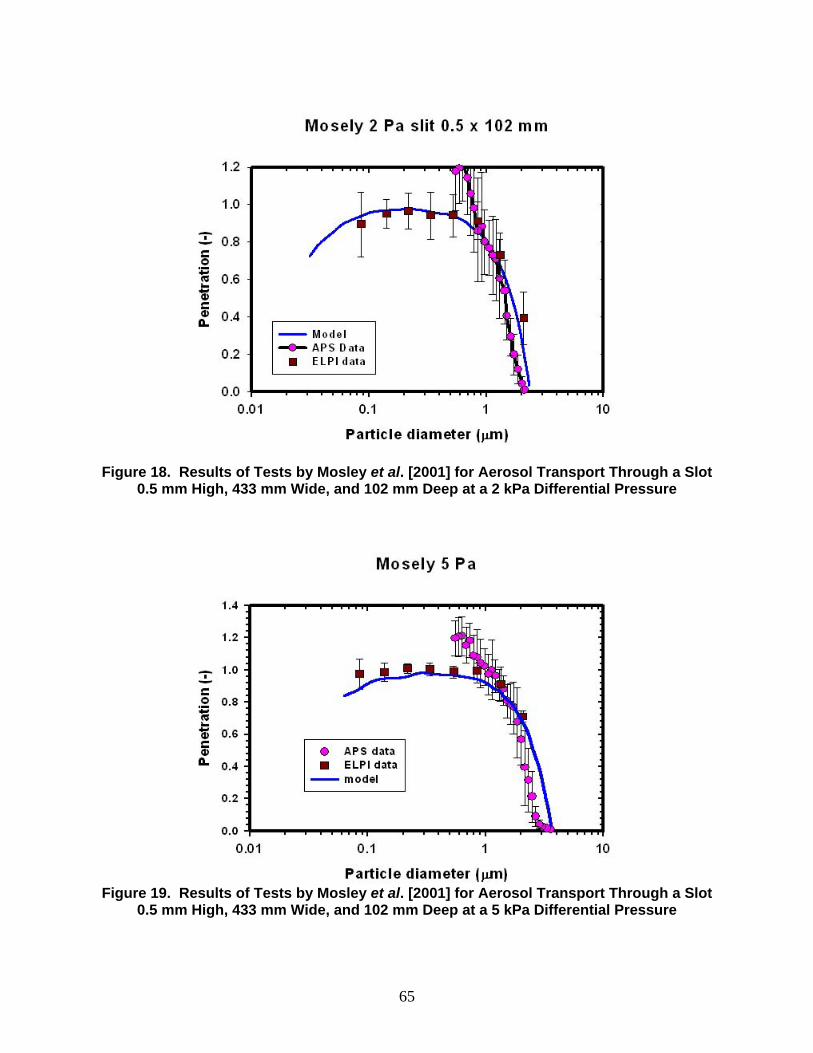
65
Figure 18. Results of Tests by Mosley et al. [2001] for Aerosol Transport Through a Slot 0.5 mm High, 433 mm Wide, and 102 mm Deep at a 2 kPa Differential Pressure
Figure 19. Results of Tests by Mosley et al. [2001] for Aerosol Transport Through a Slot
0.5 mm High, 433 mm Wide, and 102 mm Deep at a 5 kPa Differential Pressure
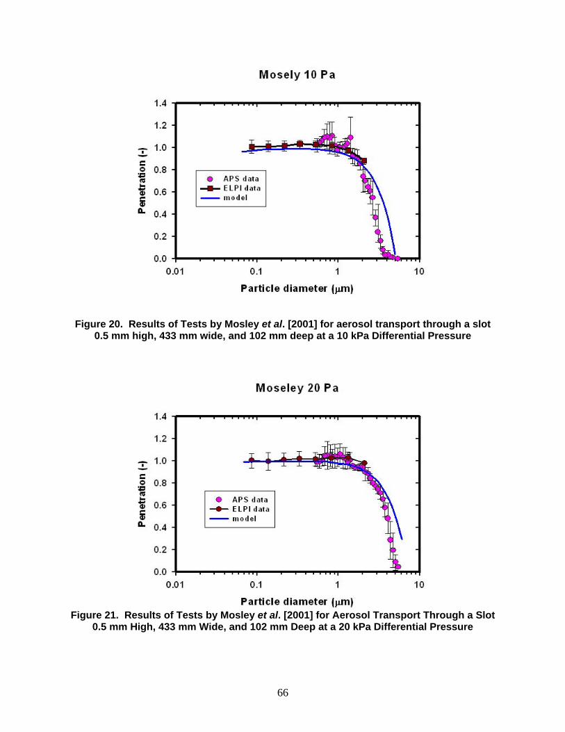
66
Figure 20. Results of Tests by Mosley et al. [2001] for aerosol transport through a slot 0.5 mm high, 433 mm wide, and 102 mm deep at a 10 kPa Differential Pressure
Figure 21. Results of Tests by Mosley et al. [2001] for Aerosol Transport Through a Slot
0.5 mm High, 433 mm Wide, and 102 mm Deep at a 20 kPa Differential Pressure
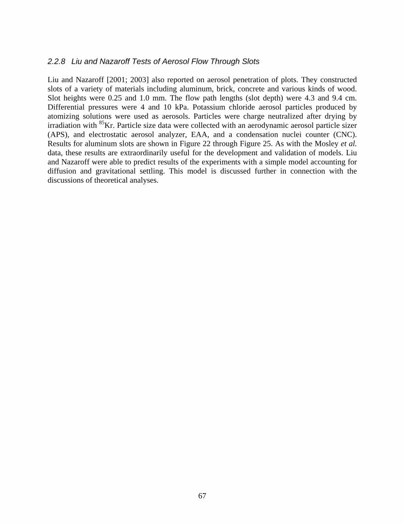
67
2.2.8 Liu and Nazaroff Tests of Aerosol Flow Through Slots Liu and Nazaroff [2001; 2003] also reported on aerosol penetration of plots. They constructed slots of a variety of materials including aluminum, brick, concrete and various kinds of wood. Slot heights were 0.25 and 1.0 mm. The flow path lengths (slot depth) were 4.3 and 9.4 cm. Differential pressures were 4 and 10 kPa. Potassium chloride aerosol particles produced by atomizing solutions were used as aerosols. Particles were charge neutralized after drying by irradiation with 85Kr. Particle size data were collected with an aerodynamic aerosol particle sizer (APS), and electrostatic aerosol analyzer, EAA, and a condensation nuclei counter (CNC). Results for aluminum slots are shown in Figure 22 through Figure 25. As with the Mosley et al. data, these results are extraordinarily useful for the development and validation of models. Liu and Nazaroff were able to predict results of the experiments with a simple model accounting for diffusion and gravitational settling. This model is discussed further in connection with the discussions of theoretical analyses.
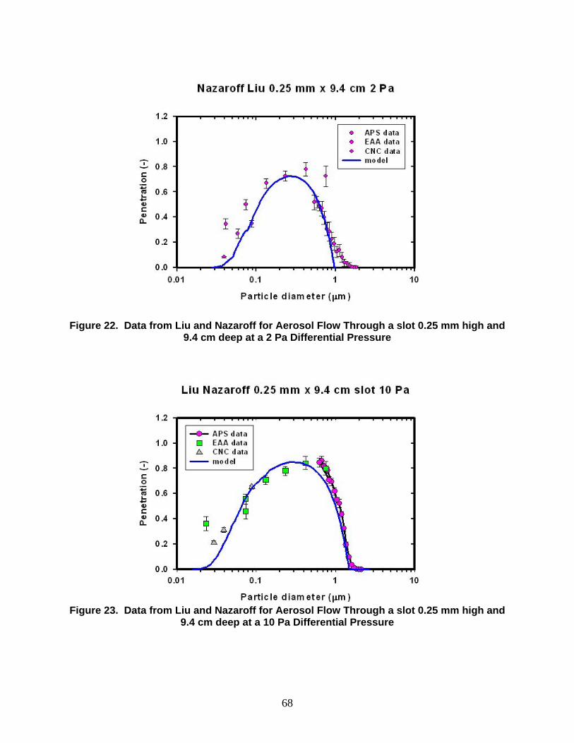
68
Figure 22. Data from Liu and Nazaroff for Aerosol Flow Through a slot 0.25 mm high and 9.4 cm deep at a 2 Pa Differential Pressure
Figure 23. Data from Liu and Nazaroff for Aerosol Flow Through a slot 0.25 mm high and
9.4 cm deep at a 10 Pa Differential Pressure
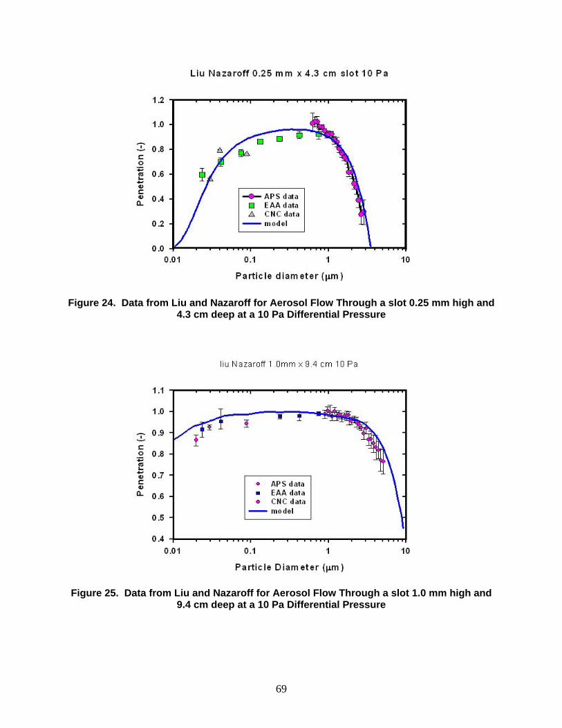
69
Figure 24. Data from Liu and Nazaroff for Aerosol Flow Through a slot 0.25 mm high and 4.3 cm deep at a 10 Pa Differential Pressure
Figure 25. Data from Liu and Nazaroff for Aerosol Flow Through a slot 1.0 mm high and 9.4 cm deep at a 10 Pa Differential Pressure
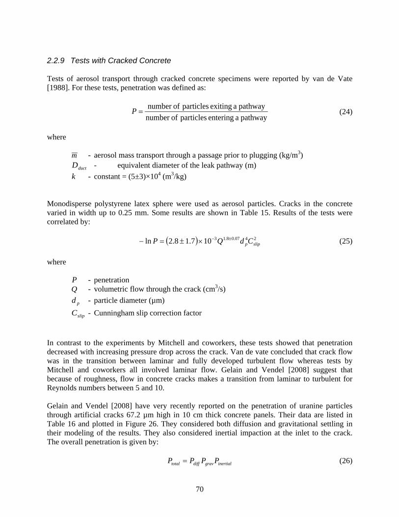
70
2.2.9 Tests with Cracked Concrete Tests of aerosol transport through cracked concrete specimens were reported by van de Vate [1988]. For these tests, penetration was defined as:
pathwaya entering particles ofnumber
pathwaya exiting particles ofnumber =P (24)
where
m - aerosol mass transport through a passage prior to plugging (kg/m3) ductD - equivalent diameter of the leak pathway (m)
k - constant = (5±3)×104 (m3/kg) Monodisperse polystyrene latex sphere were used as aerosol particles. Cracks in the concrete varied in width up to 0.25 mm. Some results are shown in Table 15. Results of the tests were correlated by: ( ) 2407.08.13107.18.2ln slippCdQP ±−×±=− (25) where
P - penetration Q - volumetric flow through the crack (cm3/s)
pd - particle diameter (µm)
slipC - Cunningham slip correction factor In contrast to the experiments by Mitchell and coworkers, these tests showed that penetration decreased with increasing pressure drop across the crack. Van de vate concluded that crack flow was in the transition between laminar and fully developed turbulent flow whereas tests by Mitchell and coworkers all involved laminar flow. Gelain and Vendel [2008] suggest that because of roughness, flow in concrete cracks makes a transition from laminar to turbulent for Reynolds numbers between 5 and 10. Gelain and Vendel [2008] have very recently reported on the penetration of uranine particles through artificial cracks 67.2 µm high in 10 cm thick concrete panels. Their data are listed in Table 16 and plotted in Figure 26. They considered both diffusion and gravitational settling in their modeling of the results. They also considered inertial impaction at the inlet to the crack. The overall penetration is given by: inertialgravdifftotal PPPP = (26)
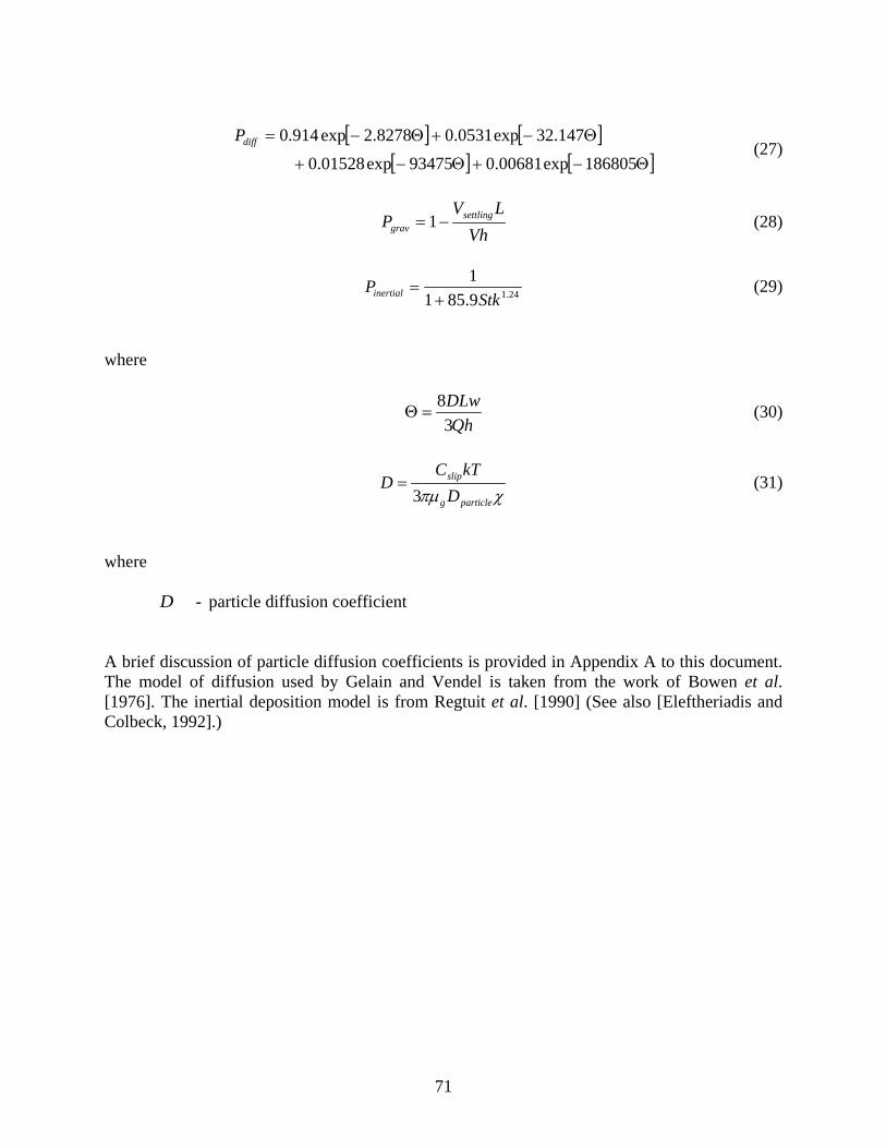
71
[ ] [ ]
[ ] [ ]Θ−+Θ−+
Θ−+Θ−=
186805exp00681.093475exp01528.0 147.32exp0531.08278.2exp914.0diffP
(27)
Vh
LVP settling
grav −= 1 (28)
24.19.8511
StkPinertial +
= (29)
where
Qh
DLw3
8=Θ (30)
χπµ particleg
slip
DkTC
D3
= (31)
where
D - particle diffusion coefficient A brief discussion of particle diffusion coefficients is provided in Appendix A to this document. The model of diffusion used by Gelain and Vendel is taken from the work of Bowen et al. [1976]. The inertial deposition model is from Regtuit et al. [1990] (See also [Eleftheriadis and Colbeck, 1992].)

72
Table 15. Penetration Observed in Transport of Polystyrene Latex Aerosols Through
Cracks in Concrete [van de Vate, 1988].
ΔP (kPa)
dp (µm)
Q (cm3/s)
Penetration (-)
3 0.48 145 0.8
3 0.82 145 0.8
3 1.1 145 0.5
3 2.0 145 0.11
6 0.48 250 0.75
6 0.82 250 0.6
6 1.1 250 0.2
6 2.0 250 0.008
9 0.48 350 0.65
9 0.82 350 0.45
9 1.1 350 0.07
9 2.0 350 0.005

73
Table 16. Uranine Particle Penetration of Cracks (h = 67.2 µm) in Concrete [Gelain
and Vendel, 2008].
Particle diameter = 1.1 µm Particle diameter = 0.8 µm Particle diameter = 0.6 µm Flow
(cm3/s) Penetration
(± 0.11) Flow
(cm3/s) Penetration
(± 0.12) Flow
(cm3/s) Penetration
(± 0.11) 51.5 0.11 85 0.57 110 0.168 51.5 0.20 85 0.35 110 0.247 111.4 0.43 85 0.30 110 0.081 134.2 0.47 128.4 0.38 230 0.255 164.6 0.48 128.4 0.44 230 0.337 183 0.30 128.4 0.64 230 0.182
236.2 0.38 171 0.71 230 0.277 390 0.21 171 0.51 230 0.359 600 0.19 260 0.46 230 0.197 341 0.480 260 0.49 230 0.305 341 0.334 260 0.52 230 0.382 380 0.501 348 0.53 230 0.182 380 0.572 360 0.33 295.3 0.435 380 0.452 360 0.44 295.3 0.510 455 0.518 475 0.36 295.3 0.354 455 0.592 500 0.51 305 0.421 455 0.466 505 0.39 305 0.505
603 0.25 305 0.348 606 0.23 330 0.439 630 0.41 330 0.515 502 0.502 330 0.365 502 0.569 341 0.408 502 0.427 519 0.423 518.5 0.452 519 0.497 518.5 0.523 519 0.349 518.5 0.381 613 0.487 613 0.554 613 0.412

74
Figure 26. Penetration of Uranine Particles Through a 67.2 µm Crack in Concrete [Gelain
and Vendel, 2008].

75
2.2.10 Tests of Leakage from a Flow Stream Most of the data cited here are for aerosol leaking from a relatively calm gas volume. Carrié and Modera [1998; 2002] examined leakage of aerosol through a slot perpendicular to a flowing steam of aerosol-laden gas (This is the so-called “transverse flow problem”.). The motivation of the investigators appears to have been the investigation of aerosols for sealing leaks in duct systems. The aerosol they used was acetate-acrylate vinyl polymer which they described as “sticky”. (At the microscopic scale of aerosol surface interactions dominated by van der Waals forces, the concept of “sticky” is difficult to quantify.) The aerosol had mass median diameters of 3 to 7 :m. The aerosol was injected into a 15 cm duct that could bent through a 3 mm high, 40 mm long slot. Gas flows were 12500 cm3/s to 55500 cm3/s at pressure differentials of 20,40, 60 and 80 Pa. The aerosols, of course, could not all follow stream lines of the flow redirection through the slot. Many would impact on the downstream wall of the slot causing the slot to narrow. An example of the change in slot thickness as a function of time is shown in Figure 27. In subsequent tests [Carrié and Modera, 2002], the authors investigated transverse flow of aerosol-laden gas through slots and joints. Some results are shown in Figure 28.

76
Figure 27. Carrié and Modera [1998] on the Variation in Slot Height Due to Aerosol Accumulation from Transverse Flow.
Figure 28. Comparison of Leakage Flow of Aerosol-Laden Gas Through a Slot and a Joint [Carrié and M.P. Modera, 2002].
For this experiment, the aerosol concentration was 0.85 g/m3. The mass median diameter of the aerosol was 3.36 µm and the geometric standard deviation was 2.49. The pressure differential was 80.7 Pa and the volumetric flow rate through the slot was 31400 cm3/s
For these tests, the aerosol had a mass median aerodynamic diameter of 4.9 µm and a geometric standard deviation of 2.7. The aerosol concentration was 0.34 ± 0.02 g/m3. The differential pressure in both tests was maintained at 200 Pa.

77
2.2.11 Multiple Bend Geometry Tests Morewitz et al. [1979] reported results of especially complicated geometry test involving about 12 bends. Typical flow pathways in the test were 0.125 cm and 0.079 cm wide. Results of the four tests were:
Test 1 Aerosol composed of a mixture of sodium oxides and sodium carbonate at a concentration of 15 to 20 g/m3 and a differential pressure of 6.9 kPa were used. The system plugged in about 5 minutes. A total of 0.217 m3 gas passed through the system and carried 3 to 4 grams of aerosol. Test 2 A similar test with 500 g/m3 sodium oxide/ sodium carbonate aerosol and a differential pressure of 280 kPa lead to plugging in about 6 seconds. Only 0.003 grams of aerosol having a means size > 6.8 :m passed through the system. Test 3 A test with uranium oxide aerosol at 900 g/m3 plugged the system in about 1.5 minutes. Gas flow through the system amounted to 0.012 m3 STP and carried 0.45 g uranium dioxide.
2.2.12 Tests of Leakage Through Containment Penetrations
Test 4 A repetition of test 3 with uranium dioxide aerosol at 230 g/m3 lead to plugging in about 5 minutes. Gas flow through the system was 0.013 m3
STP. About 0.015 g
of uranium oxide aerosol was carried through the system.
Watanabe et al. [unpublished] described results of an integral test of aerosol leakage through boiling water reactor containment penetrations. A large model BWR containment was heated. The atmosphere of the containment was contaminated with CsI aerosol. At 553 to 593 K, leakage was detected in a low voltage electrical penetration. The pressure differential across the penetration at the time leakage was detected was about 7 kPa. The aerosol concentration within the model was about 0.08 g/m3. The aerosol had a mass median aerodynamic diameter of about 1.4 :m. At the outlet side of the penetration aerosol concentrations were 0.003 to 0.005 g/m3. With time, the decontamination of aerosol-laden gas passing through the electrical penetration increased by about a factor of 3. Continued heating of the model containment lead to leakages in the flange gasket when temperatures reached 803 to 633 K. Post test examination showed that the gasket on the flange had developed cracks up 10 mm wide. Decontamination factors for aerosol-laden gas passing through these cracks was found to vary between 10 and 30.

78
For neither the electrical penetration leakage nor the flange gasket leakage are their data on the size dependence of decontamination. Consequently, extrapolating the integral test results to other situations is difficult. 2.2.13 Containment Leak Tests Hilliard and Postma [1981] reported results obtained in a series of large scale containment leak tests. For these tests, deliberate leaks were introduced that passed 0.1 to 1.0 liters of aerosol-laden gas per minute. The authors defined an “attenuation factor”, Af to be:
pathwayleak theentering mass
leak the throughpassing mass=fA (32)
They considered leakage of cesium particles and iodine in both gaseous and particle form. The cesium particles had aerodynamic settling diameters of 10-17 µm in the early stages of the tests. The mean settling diameters were between 3 and 10 µm in the late stages of the test. The geometry of the leak path was quite complicated and included a needle valve, so analysis of the tests would be challenging. They reported attenuation factors at 2 and 24 hours. But, these attenuation factors apparently included the effect of condensation in a volume beyond the needle valve and the subsequent heat up of the condensate to dryness. The authors reported that ~96% of the iodine and ~99% of the cesium were retained in the heated volume as a nonvolatile residue as though most of the iodine and cesium had successfully negotiated passage through the leak and the needle valve only to be trapped in condensate.
79
2.3 Turbulent Deposition of Particles Many of the experiments described in the previous section of this report have been analyzed assuming the flow is laminar and the primary deposition mechanisms are gravitational for larger particles and diffusive for smaller particles. Turbulent flow conditions can develop especially in flow through cracks in concrete where surface roughness can trigger turbulence. Turbulence introduces a new mechanism for the deposition of aerosol particles. This mechanism is a very local phenomenon. Aerosol deposition is not usually analyzed in terms of “penetration”. Rather, turbulent particle deposition is usually considered in terms of a deposition velocity Vd. The deposition velocity relates the particle flux, in terms of either mass or particle number, to the particle concentration in the gas phase, again either in terms of mass concentration or number concentration:
CVdtdN
A d=1 (33)
where
dV - deposition velocity C - particle concentration
In early work on turbulent aerosol deposition, it was assumed that the deposition velocity could be correlated with flow conditions via some function of the Reynolds number. Experimental evidence has shown there to be a confounding between the flow conditions and the particle properties. It is now common to correlated the deposition velocity with the particle relaxation time, τ. The particle relaxation time is defined and discussed in Appendix A. Dimensionless quantities used in the correlation are:
*uVV d
d =+ (34)
( )
g
g uµ
τρτ
2*
=+ (35)
where
*u - friction velocity For flow through smooth cylindrical channels, the friction velocity is found from:

80
2
* fVu = (36)
41Re0791.0
=f (37)
g
gpath VDµρ
=Re (38)
where
pathD -diameter of cylindrical pathway Where the flow pathway is not perfectly cylindrical, it is common to use the hydraulic diameter as discussed above in Section 2.1. Turbulent deposition data of interest for common idealizations of cylindrical leaks involves deposition on smooth surfaces. (Concrete cracks are, of course, an exception.) A vast amount of data has been gathered on turbulent deposition in such pathways. Most has been from experiments larger than those of interest for leaks from reactor containment buildings, but the dimensionless correlation of deposition velocity and particle relaxation time makes it possible to apply these data. The objective here is to accumulate this data base, at least, to an appreciable extent. The experimental data base has been reviewed many times [Parker et al., 2008; Papavergos and Hedley, 1984; and especially Sippola and Nazaroff, 2002]. Consequently, only very brief descriptions of important experimental studies are provided in the subsections that follow. To avoid too much more disruption of the flow of the text, tabulated values of the dimensionless deposition velocity and dimensionless particle relaxation times derived from the experiment data are collected in Appendix B.

81
2.3.1 Friedlander and Johnstone The experimental studies conducted by Friedlander and Johnstone [1957] is usually considered the work that initiated 50 years of investigation of turbulent deposition of aerosol. Prior investigations had been reported, but Friedlander and Johnstone provided a mechanistic interpretation of their experimental observations. The experiments were done with a variety of particles in vertical tubes of various types. Data derived by digitizing plots in the Friedlander and Johnstone publication are shown in Figure 29.These data are now considered to be of primarily historical significance though they are occasionally still cited in the validation of theoretical models of turbulent deposition.
Figure 29. Turbulent Aerosol Particle Deposition Data Obtained by Friedlander and Johnstone [1957].
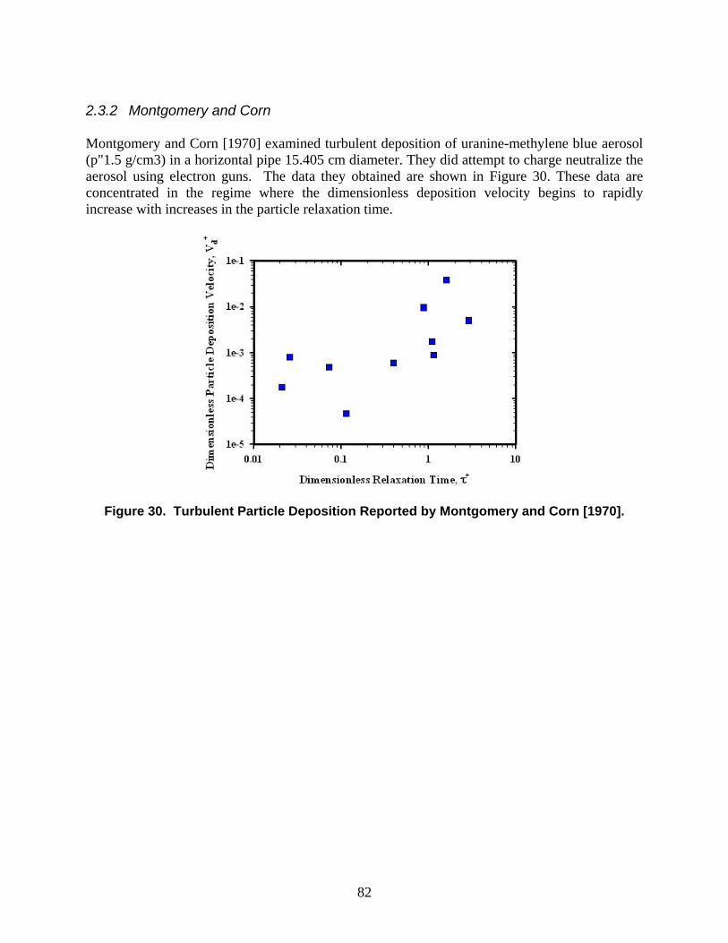
82
2.3.2 Montgomery and Corn Montgomery and Corn [1970] examined turbulent deposition of uranine-methylene blue aerosol (p"1.5 g/cm3) in a horizontal pipe 15.405 cm diameter. They did attempt to charge neutralize the aerosol using electron guns. The data they obtained are shown in Figure 30. These data are concentrated in the regime where the dimensionless deposition velocity begins to rapidly increase with increases in the particle relaxation time.
Figure 30. Turbulent Particle Deposition Reported by Montgomery and Corn [1970].

83
2.3.3 Wells and Chamberlain Wells and Chamberlain [1967] reported data on the deposition of tricresyl phosphate droplets (density = 1.16 g/cm3). They used a vertical, copper duct with flow downwards. The deposition surface was a brass rod 1.27 cm in diameter within the 3.81 cm diameter duct. Their data shown in Figure 31 are concentrated in the regime of dimensionless droplet relaxation times where the dimensionless deposition velocity passes through a minimum.
Figure 31. Turbulent Deposition of Tricresyl Phosphate Droplets [Wells and Chamberlain, 1967].

84
2.3.4 Liu and Agarwal Widely considered a definitive study, the data obtained by Liu and Agarwal [1974] are frequently used to substantiate theoretical models of turbulent deposition of aerosols. The data were obtained using olive oil particles (density = 0.92 g/cm3) tagged with uranine. The experiments were done with a vertically oriented glass tube 1.27 cm in diameter. Air was the gas phase in these tests. Results of the tests are shown in Figure 32. There is a sharp rise in the dimensionless deposition velocity for values of the dimensionless particle relaxation time of 0.2 to about 10. Thereafter, the dimensionless deposition velocity slowly decreases with increases in the dimensionless particle relaxation time. This slow decrease is thought to be real and not an artifact of particle bounce.
Figure 32. Turbulent Particle Deposition Data from Liu and Agarwal [1974 ] and from El-
Shobokshy [1983].
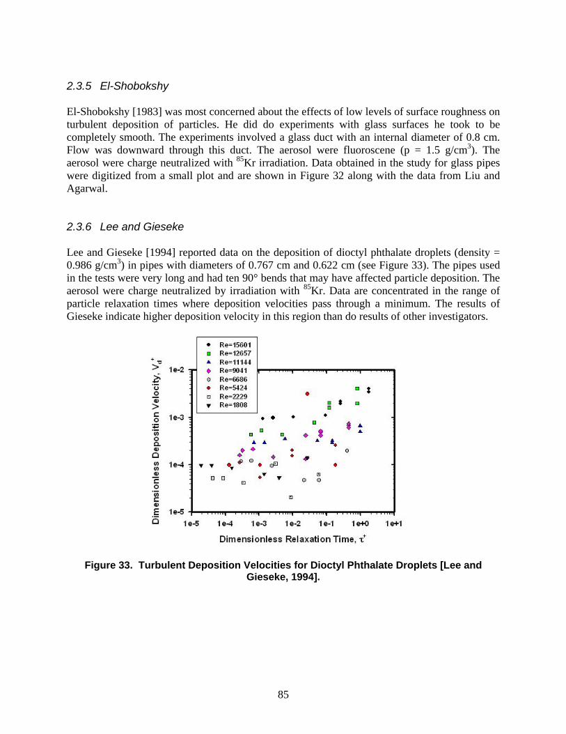
85
2.3.5 El-Shobokshy El-Shobokshy [1983] was most concerned about the effects of low levels of surface roughness on turbulent deposition of particles. He did do experiments with glass surfaces he took to be completely smooth. The experiments involved a glass duct with an internal diameter of 0.8 cm. Flow was downward through this duct. The aerosol were fluoroscene (p = 1.5 g/cm3). The aerosol were charge neutralized with 85Kr irradiation. Data obtained in the study for glass pipes were digitized from a small plot and are shown in Figure 32 along with the data from Liu and Agarwal. 2.3.6 Lee and Gieseke Lee and Gieseke [1994] reported data on the deposition of dioctyl phthalate droplets (density = 0.986 g/cm3) in pipes with diameters of 0.767 cm and 0.622 cm (see Figure 33). The pipes used in the tests were very long and had ten 90° bends that may have affected particle deposition. The aerosol were charge neutralized by irradiation with 85Kr. Data are concentrated in the range of particle relaxation times where deposition velocities pass through a minimum. The results of Gieseke indicate higher deposition velocity in this region than do results of other investigators.
Figure 33. Turbulent Deposition Velocities for Dioctyl Phthalate Droplets [Lee and Gieseke, 1994].

86
2.3.7 Shimada et al. Shimada et al. [1993] reported data on the deposition of extremely fine aerosol particles (0.01 to 0.043 µm) (see Figure 34). Unfortunately, the composition of the particles is not stated in their publication. Based on other work by the authors [Kuyama et al., 1984], it suspected that the particles are sodium chloride (density = 2.165 g/cm3). The experiments were done with a horizontal copper pipe (ID = 0.6 cm) using air as the gas phase. The investigators did charge neutralize their aerosol. Reynolds numbers for the flow velocity went up to ~50,000.
Figure 34. Turbulent NaCl Aerosol Deposition Data from Shimada et al. [1993].
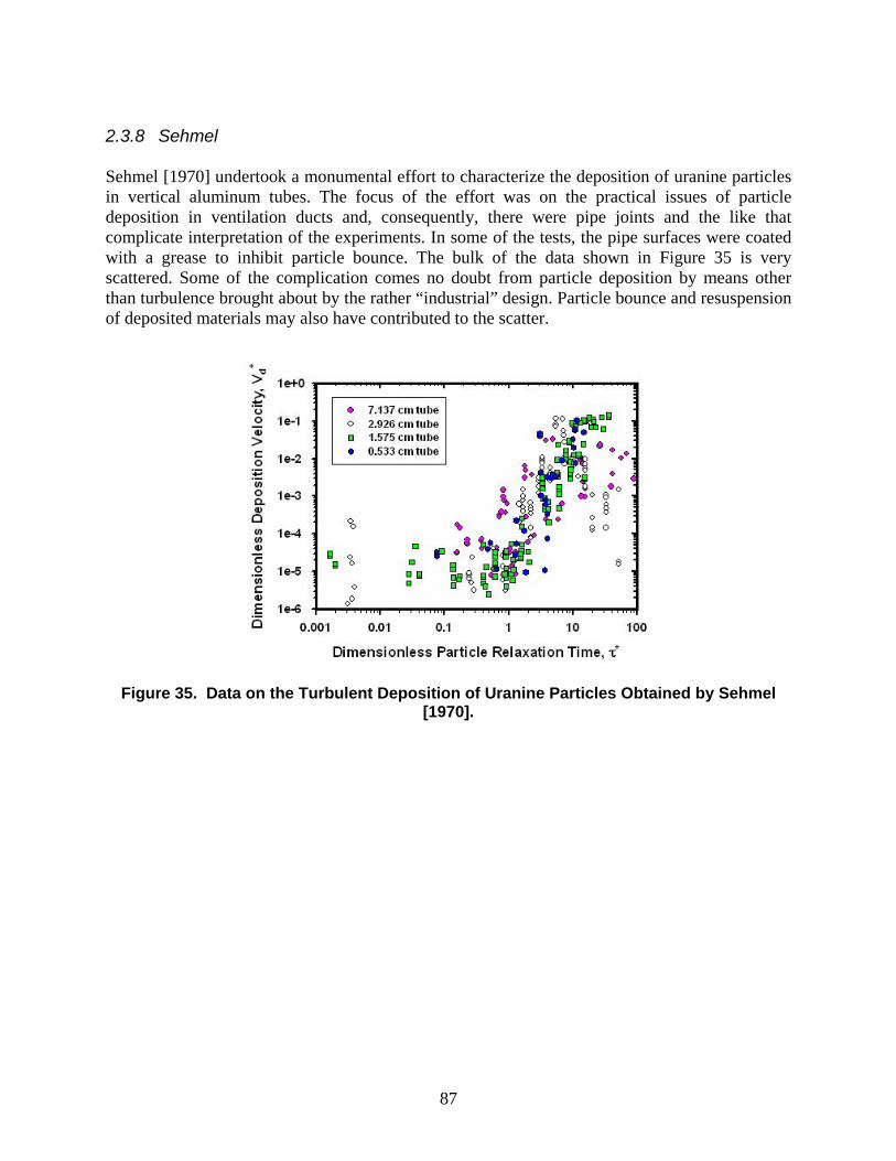
87
2.3.8 Sehmel Sehmel [1970] undertook a monumental effort to characterize the deposition of uranine particles in vertical aluminum tubes. The focus of the effort was on the practical issues of particle deposition in ventilation ducts and, consequently, there were pipe joints and the like that complicate interpretation of the experiments. In some of the tests, the pipe surfaces were coated with a grease to inhibit particle bounce. The bulk of the data shown in Figure 35 is very scattered. Some of the complication comes no doubt from particle deposition by means other than turbulence brought about by the rather “industrial” design. Particle bounce and resuspension of deposited materials may also have contributed to the scatter.
Figure 35. Data on the Turbulent Deposition of Uranine Particles Obtained by Sehmel [1970].
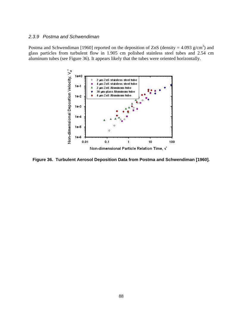
88
2.3.9 Postma and Schwendiman Postma and Schwendiman [1960] reported on the deposition of ZnS (density = 4.093 g/cm3) and glass particles from turbulent flow in 1.905 cm polished stainless steel tubes and 2.54 cm aluminum tubes (see Figure 36). It appears likely that the tubes were oriented horizontally.
Figure 36. Turbulent Aerosol Deposition Data from Postma and Schwendiman [1960].
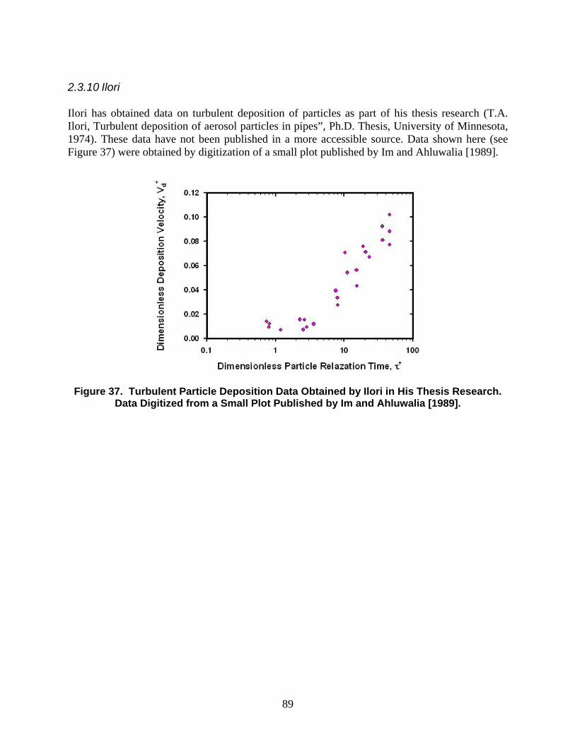
89
2.3.10 Ilori Ilori has obtained data on turbulent deposition of particles as part of his thesis research (T.A. Ilori, Turbulent deposition of aerosol particles in pipes”, Ph.D. Thesis, University of Minnesota, 1974). These data have not been published in a more accessible source. Data shown here (see Figure 37) were obtained by digitization of a small plot published by Im and Ahluwalia [1989].
Figure 37. Turbulent Particle Deposition Data Obtained by Ilori in His Thesis Research. Data Digitized from a Small Plot Published by Im and Ahluwalia [1989].
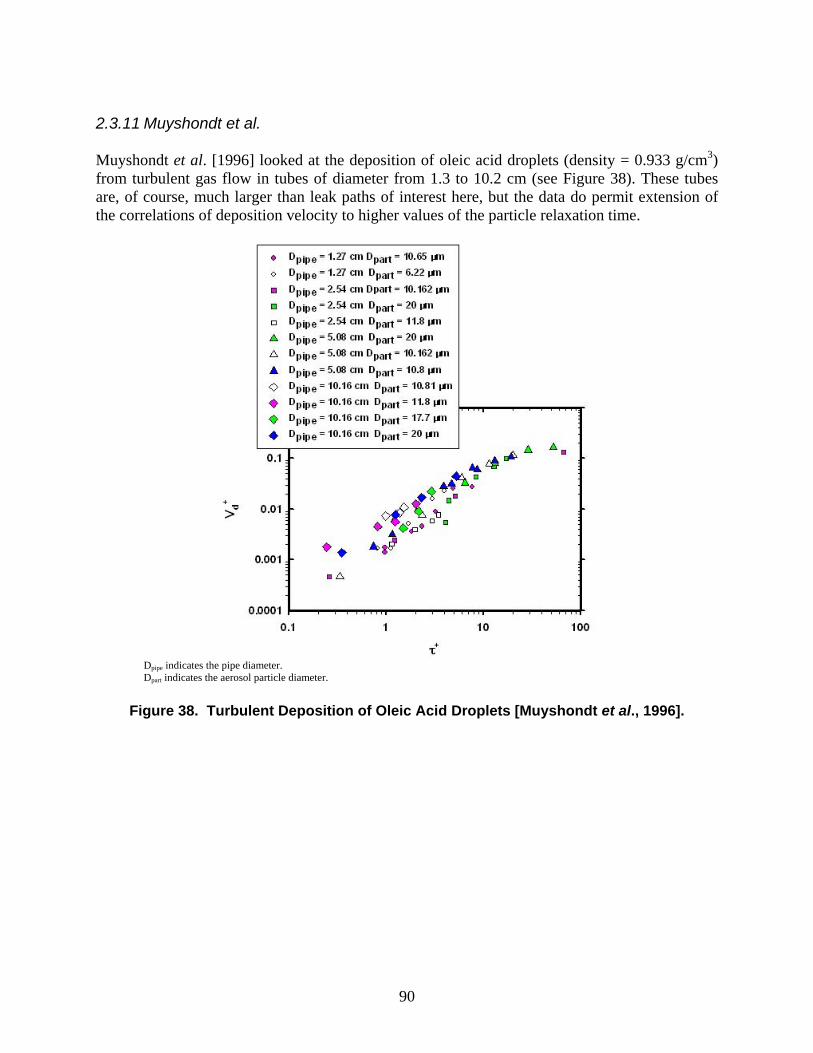
90
2.3.11 Muyshondt et al. Muyshondt et al. [1996] looked at the deposition of oleic acid droplets (density = 0.933 g/cm3) from turbulent gas flow in tubes of diameter from 1.3 to 10.2 cm (see Figure 38). These tubes are, of course, much larger than leak paths of interest here, but the data do permit extension of the correlations of deposition velocity to higher values of the particle relaxation time.
Dpipe indicates the pipe diameter. Dpart indicates the aerosol particle diameter.
Figure 38. Turbulent Deposition of Oleic Acid Droplets [Muyshondt et al., 1996].

91
2.3.12 Forney and Spielman Forney and Spielman [1974] examined the deposition of lycopedium spores (mean diameter = 30.9 Im; density " 0.65 g/cm3), ragweed pollen (mean diameter = 19.5 µm; density " 0.48 g/cm3) and pecan pollen (mean diameter = 48.5 µm; density " 0.94 g/cm3) from turbulent flow in vertically oriented cylinders with internal diameters of 1.3, 1.78, 2.54, 3.12, 3.65, and 4.4 cm (see Figure 39). The particles they used were, of course, far larger than aerosols that are of interest for the purposes of reactor accident analyses. The large particles do allow the data base for turbulent deposition of particles to be expanded. Forney and Spielman encountered severe particle bounce problems at values of the dimensionless particle relaxation time in excess of about 10. They attempted to counter the tendency for particles to bounce off the tube walls by coating these walls with petroleum jelly is widely done in the aerosol field. This helped, but did not eliminate particle bounce. The investigators found that a mixture of 75% paraffin oil and 25% petroleum jelly sufficiently suppressed particle bounce for their purposes.
Blue squares are data for Lycopodium spores. Light blue triangles are data for Pecan pollen particles. Green circles are data for ragweed pollen particles
Figure 39. Data on Turbulent Deposition of Large Particles [Forney and Spielman, 1974]. An overall plot of several of the data sets discussed above is shown in Figure 40. Data extend over about 7 orders of magnitude in the value of the dimensionless particle relaxation time. The dimensionless deposition velocity decreases with increasing relaxation time in the regime where diffusion is an important process for bringing particles into contact with the surfaces. When the dimensionless relaxation time reaches a value of about 0.1, the dimensionless deposition velocity increases quite abruptly even in the logarithmic scale of the plot to a maximum at a relaxation time of about 30. There is a slow decrease in the deposition velocity with increases in the

92
relaxation time beyond that maximum. There are theoretical reasons to think that this slow decrease is a manifestation of the turbulent process and not the product of particle bounce [Sipolla and Nazaroff, 2002].
Figure 40. Turbulent Particle Deposition Data from Several Investigations.

93
3. THEORETICAL INVESTIGATIONS Particles that enter leak pathways are susceptible to several processes that can lead to deposition. The processes listed by van de Vate in his studies of aerosol leakage through concrete cracks are:
• Diffusion • Electrophoresis • Thermophoresis • Diffusiophoresis • Gravitational settling • Inertial impaction and interception
To this list, Williams [1994] would add advection and turbophoresis. Van de Vate [1988] has assessed the importance of each of the mechanisms within the context of aerosol transport through cracked concrete. He is able to discount thermophoresis and diffusiophoresis despite the pressure drop across the leak path. Diffusion, including where applicable turbulent diffusion, gravitational settling and inertial impaction, again where applicable, emerge as the dominant mechanisms of aerosol deposition. Since publication of the Morewitz-Vaughan correlation, there has been substantial theoretical work on aerosol transport. Much of the pertinent work has been directed at accounting for the simplicity of the empirically derived correlation. (Earlier theoretical work has been well reviewed by Schwendiman and Sutter [1997].) Deposition data show a strong variation between laminar and turbulent flow conditions. Modeling activities also divide naturally between these two flow regimes. 3.1 Laminar Flow Conditions The utility of rather simple flow models for aerosol deposition from laminar flows through leak pathways has been demonstrated by results reported by Mosley et al. [2001] and by Liu and Nazaroff [2003] and discussed in Section 3. Both of these teams of investigators have assumed that deposition is dominated by diffusion and gravitational settling. They assume further that these processes operate independently so that the overall penetration is given by the product of penetrations achieved by either mechanism alone: gravdiffoverall PPP = (39) Were inertial impaction important in the tests these investigators examined, its effects could be included as a third term in the product on the right hand side of this equation. Both sets of investigators use the Fuchs model for the penetration that will be achieved in the face of just gravitational settling: where:

94
hV
LVP settling
grav −= 1 (40)
where
settlingV - settling velocity of the aerosol particle L - depth of the leak passage diameter of the leak pathway (m) h - height of the leak passage (note that some analysts use 2h as the leak height) V - flow velocity through the leak
To model penetration when only diffusion leads to particle deposition, Mosley et al. use the expression:
( )
=
VhL
P pdiff 22
967.1exp
η (41)
where
pη - particle diffusion coefficient = pg
slip
dkTCπµ3
k - Boltzmann constant slipC - Cunningham slip correction factor
pd - particle diameter Liu and Nazaroff, on the other hand, use [De Marcus and Thomas, 1952]: ( ) ( ) ( )φφφ 152exp3.22exp592.0885.1exp915.0 −+−+−=diffP (42) where
VhLp
2
4ηφ = (43)
Liu and Nazaroff related pressure differential across the slots used in their test to volumetric flow using an equation by Baker [1987]:

95
222arg
3 212
Qwh
CQ
whL
P edischgg ρµ+=∆ (44)
where the discharge coefficient is given by bendedisch nC += 5.1arg (45) and where
bendn - number of right angle bends in the crack For diffusive deposition, Schwendiman and Sutter [1977] prefer:
( ) ( ) ( )( ) ( )φφ
φφφ
750exp025.0123exp027.0 57exp032.023exp097.065.3exp819.0
−+−+
−+−+−=diffP (46)
which has been validated by Sinclair et al. [1976] For small values of φ (< 0.1), some prefer the Gormley and Kennedy expression [1949]: 333.1667.0 177.02.156.21 φφφ ++−=diffP (47) Differences in the detailed expressions for penetration when diffusion is the only process leading to diffusion do not make large differences in the predictions for experiments since the fraction of particles subject to rapid diffusive deposition is small typically. Schwendiman and Sutter also note the expressions derived by Browning and Ackley [1963] for the decontamination factor (DF) – the reciprocal of penetration) associated with flow through circular and rectangular channels:
• circular channel
2
2
10 2.2030867.0logPD
LDF pg
∆+=
ηµ (48)
• rectangular channel
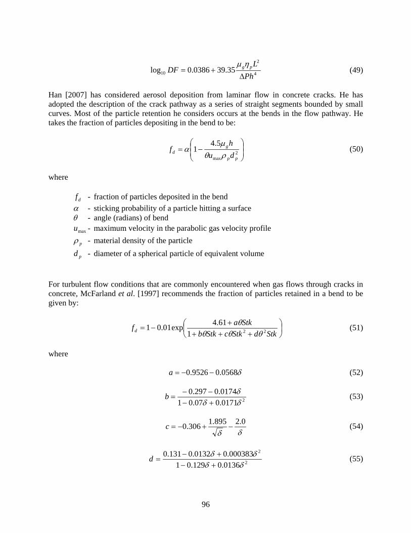
96
4
2
10 35.390386.0logPh
LDF pg
∆+=
ηµ (49)
Han [2007] has considered aerosol deposition from laminar flow in concrete cracks. He has adopted the description of the crack pathway as a series of straight segments bounded by small curves. Most of the particle retention he considers occurs at the bends in the flow pathway. He takes the fraction of particles depositing in the bend to be:
−= 2
max
5.41
pp
gd du
hf
ρθµ
α (50)
where
df - fraction of particles deposited in the bend α - sticking probability of a particle hitting a surface θ - angle (radians) of bend
maxu - maximum velocity in the parabolic gas velocity profile
pρ - material density of the particle
pd - diameter of a spherical particle of equivalent volume For turbulent flow conditions that are commonly encountered when gas flows through cracks in concrete, McFarland et al. [1997] recommends the fraction of particles retained in a bend to be given by:
++++
−=StkdStkcStkb
Stkafd 22161.4exp01.01
θθθθ (51)
where δ0568.09526.0 −−=a (52)
20171.007.010174.0297.0
δδδ
+−−−
=b (53)
δδ0.2895.1306.0 −+−=c (54)
2
2
0136.0129.01000383.00132.0131.0
δδδδ
+−+−
=d (55)

97
h
Rbend2=δ (56)
χµ
ρh
VdCStk
g
ppslip
9
2
= (57)
and where
bendR - radius of the bend in the flow path 3.2 Chen Yu Method for Deposition by Multiple Mechanisms Many of the models of aerosol deposition in leak pathways treat the deposition by multiple mechanisms as independent processes. The overall penetration is simply the product of penetration that would be produced if each mechanism operated alone. The efficiencies of deposition (logarithms of penetration) are simply additive. This works well when diffusion and gravitational deposition are the only important mechanisms since these mechanisms are most effective on distinct portions of any real aerosol size distribution. Inertial deposition, on the other hand, operates on particles that are also affected by one or the other of diffusion or gravitational settling. The efficiencies of deposition are not simply additive. Logically, a proper method for combining efficiencies is: ( )( ) 212121 111 εεεεεεε −+=−−−=overall (58) where 1ε and 2ε are the efficiencies of each process when it operates alone. Chen and Yu [1993] argue that a better way to combine efficiencies of two mechanisms is:
( )22122
21 εεεεε −+=overall (59)
Similar, but more complicated, expressions are provided for three mechanisms: ( ) ( ) ( ) ( )2321
232
231
221
23
22
21 εεεεεεεεεεεεε −−−−++=overall (60)
Chen and Yu also provide expressions for the efficiencies of aerosol deposition by diffusion and gravitational sedimentation in plug and parabolic flows: Sedimentation - slug flow [Yu et al., 1977]
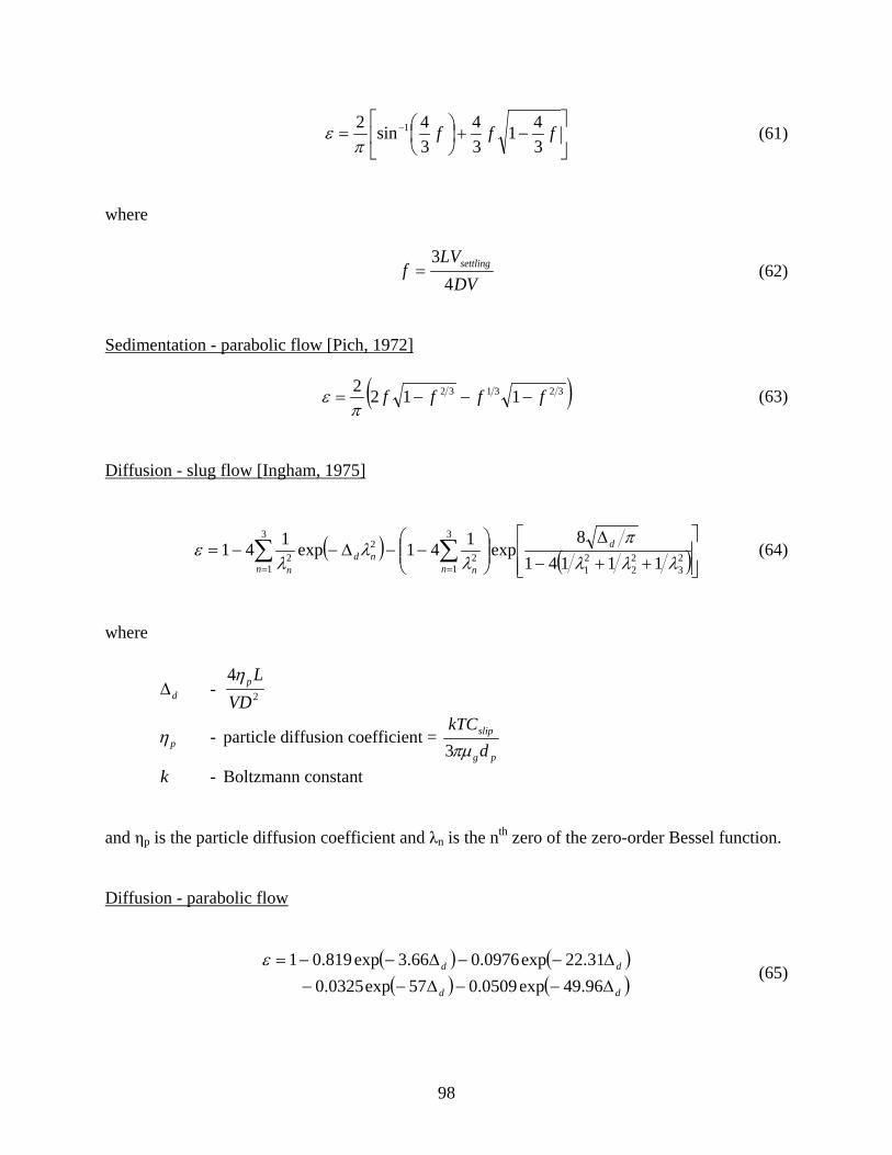
98
−+
= − fff
341
34
34sin2 1
πε (61)
where
DV
LVf settling
43
= (62)
( )323132 1122 ffff −−−=π
ε
Sedimentation - parabolic flow [Pich, 1972]
(63)
( ) ( )
++−∆
−−∆−−= ∑∑
==23
22
21
3
12
3
1
22 11141
8exp141exp141
λλλπ
λλ
λε d
n nnnd
n
Diffusion - slug flow [Ingham, 1975]
(64)
where
d∆ - 2
4VD
Lpη
pη - particle diffusion coefficient = pg
slip
dkTCπµ3
k - Boltzmann constant and ηp is the particle diffusion coefficient and λn is the nth zero of the zero-order Bessel function.
( ) ( )( ) ( )dd
dd
∆−−∆−−∆−−∆−−=
96.49exp0509.057exp0325.0 31.22exp0976.066.3exp819.01ε
Diffusion - parabolic flow
(65)

99
Chen and Yu draw a distinction between fully developed laminar flow with a parabolic gas velocity profile across the pathway and plug flow where the gas velocity profile is flatter. In real capillaries, gas entering a capillary will have a velocity profile approximating the flat profile of plug flow more or less depending on details of the inlet. This velocity profile will evolve over the entry length to become parabolic. Mass (and heat transfer) is somewhat slower from fully developed laminar flow with a parabolic velocity profile than it is in plug flow. The somewhat faster mass transfer in the inlet region to a capillary may be one of the reasons that aerosol deposition is often seen to begin at the entrance to a capillary.

100
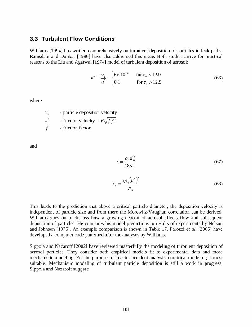
101
3.3 Turbulent Flow Conditions Williams [1994] has written comprehensively on turbulent deposition of particles in leak paths. Ramsdale and Dunbar [1986] have also addressed this issue. Both studies arrive for practical reasons to the Liu and Agarwal [1974] model of turbulent deposition of aerosol:
><×
==+
+−
+
9.12for 1.09.12for 106 4
* ττ
uvv d (66)
where
dv - particle deposition velocity *u - friction velocity = 2fV
f - friction factor
and
g
pd dµ
ρτ
18
2
= (67)
( )
g
d uµ
τρτ2*
=+ (68)
This leads to the prediction that above a critical particle diameter, the deposition velocity is independent of particle size and from there the Morewitz-Vaughan correlation can be derived. Williams goes on to discuss how a growing deposit of aerosol affects flow and subsequent deposition of particles. He compares his model predictions to results of experiments by Nelson and Johnson [1975]. An example comparison is shown in Table 17. Parozzi et al. [2005] have developed a computer code patterned after the analyses by Williams. Sippola and Nazaroff [2002] have reviewed masterfully the modeling of turbulent deposition of aerosol particles. They consider both empirical models fit to experimental data and more mechanistic modeling. For the purposes of reactor accident analysis, empirical modeling is most suitable. Mechanistic modeling of turbulent particle deposition is still a work in progress. Sippola and Nazaroff suggest:

102
( ) ( )
( )
>
≥
<
=
+++
+
++
+
270for 50-12.618.0,for 18.018.0,for Sc,
τττ
τ
ττ
ScfScff
vd (69)
where
( ) ( )2432 105.3063.0, +−+ ×+= ττ
ScScf (70)
partd
g
DSc
ρµ
= (71)
and where
D - particle diffusion coefficient (see Appendix A)

103
Tabl
e 17
. C
ompa
rison
of W
illia
ms
Turb
ulen
t Dep
ositi
on M
odel
to R
esul
ts o
f Tes
ts b
y N
elso
n an
d Jo
hnso
n.
E
xper
imen
t
M
odel
Pre
dict
ion
Insi
de
diam
eter
(c
m)
Len
gth
(cm
) ae
roso
l con
c.
(g/m
3 ) ga
s flo
w
(cm
3 ) Pl
ug M
ass
(mg)
Pl
ug ti
me
(min
) Pl
ug ti
me
(min
) ga
s flo
w
(cm
3 ) Pl
ug M
ass
(mg)
0.05
2 4.
9 15
-11
60
0.65
-0.9
0.
1-0.
15
0.46
12
0 1.
48
0.05
2 4.
9 12
.5-9
.5
120
1.3-
1.5
2.2-
2.9
0.54
14
0 1.
48
0.05
2 4.
9 10
-7
140
1.0-
1.4
1.5-
3.1
0.7
180
1.48
0.
052
4.9
4.2-
2.8
25
0.7-
1.0
2.9-
4.3
1.7
440
1.48
0.
052
4.9
1.3-
0.9
1500
1.
4-1.
9 25
5.
4 14
00
1.48
0.
052
4.9
1.9-
0.04
7
no p
lug
0.08
7.
6 5.
8 16
0 0.
93
0.3
1.58
96
0 5.
4 0.
08
7.6
4.4
160
0.88
1.
1-1.
5 2.
1 13
00
5.4
0.08
7.
6 1.
5-1.
25
1070
1.
5 6.
5-7.
5 6.
65
4100
5.
4 0.
08
7.6
0.26
-0.1
7 56
00
1.3
21-3
1 42
.7
2600
0 5.
4 0.
08
7.6
0.13
0.00
01
no
plu
g
0.
107
3.8
0.75
-1.6
55
00
14.3
10
-14
3.65
52
00
11.2
0.
107
7.6
0.4
1700
0 19
.4
33-3
6 9.
6 11
300
12.8
0.
107
3.8
0.7
2000
0 9.
5 39
16
.8
2420
0 11
.1
0.10
7 7.
6 20
-2.5
no p
lug
0.10
7 7.
6 0.
14
0.00
01
no
plu
g
0.13
2 3.
8 9-
9.8
1000
0 92
23
-24
1.15
27
00
19.1
0.
132
7.6
1.3-
6.2
3100
0 95
39
-41
3.5
6700
23
.6
0.15
7 7.
6 15
-18
3500
58
4
0.9
2600
38
.4
0.15
7 7.
6 8-
21
no
plu
g

104

105
3.4 Other Considerations Much of the discussion of the theoretical and experimental aspects of particle deposition in leak pathways has been based on the presumption that a particle impacting a surface will be retained permanently on that surface. This need not be the case. Particle can bounce off surface and particles deposited on surfaces can resuspend in the flow. Bounce has afflicted many attempts to measure turbulent deposition of solid particles when measures were not taken to suppress bounce such as coating surfaces with grease or oil. (Liquid droplets appear less susceptible to bounce but they are not immune.) Particle resuspension was observed in tests done by Mitchell and coworkers as discussed in Section II.B of this report. It appears that Van de Vate may have observed resuspension in tests of aerosol retention in cracks in concrete. Particle bounce is incompletely understood. Dahneke [1995] has discussed the normal impact of fully dense, spherical particles on a flat surface and derived an expression for the critical impact velocity necessary for particles to bounce from the surface:
−= 112
2emAVp
bounce (72)
where
e - coefficient of restitution of the particle A - particle-surface interaction energy
The critical velocity depends explicitly on the coefficient of restitution of the particle material and the energy of interaction with the surface material. Neither of these will be well known for the aerosols of interest in the analysis of reactor accidents. Furthermore, the bounce of particles from surfaces also depends on angle of particle impact with the surface [Xu et al., 1993], surface roughness [Tsai et al., 1990] and the yield strengths of both the particle material and the surface material [John, 1995]. Ellenbecker et al. [1980] have suggested that for real applications the concept of a critical velocity for particle bounce is not as useful as the idea that there is a probability that a particle will bounce upon impact with a surface. Further, the probability can be related to the kinetic energy of the particle based on the component of velocity normal to the gross surface geometry. The many uncertain factors that affect bounce will in real situations have distributions of values. These distributions are unknown, of course. But, appeal to the Central Limit Theorem suggests that distributed values of important factors affecting bounce will lead to a lognormal probability of particle bounce:
∫∞
∞−
−= dyyPbounce
2
21exp
21π
(73)

106
where
σln
ln41
= oKEKE
z (74)
2
21
npvmKE = (75)
and
pm - particle mass
nv - particle velocity normal to the surface Using the data from Ellenbecker et al. to parameterize this model yields:
J 10484.4 14−×=oKE 189.4=σ
Predictions of this model are compared in Figure 41 with data for the probability of fly ash particle bounce from filter beds. Note that the data from Löffler [1974] and from Esmen et al. [1978] were not used in the parameterization of the model. Though the model does not conform well to any of the individual data sets, in aggregate it does appear to reflect the observations. The model predicts it to be more likely that big particles will bounce than small particles. Furthermore, it is quite difficult to have all particles of the size of interest for reactor accident to bounce. The generality of the model and certainly the parameterization of the model cannot be assured, but the approach to prediction of particle bounce appears promising. The model does not account for all pertinent phenomena. For example, there is assuredly some impact velocity that will cause particle to break and fragment rather than simply bounce [Thronton et al., 1996]. Resuspension will lift particles deposited on surfaces back into the flow through the leak pathway. Resuspension of deposited aerosol has received some study in recent years [Biasi, et al., 2001; Reeks and Hall, 2001]. These studies have focused on resuspension induced by sudden changes in the gas flow over the deposited particles. The investigations show that there can be a sudden large resuspension. This immediate resuspension is followed by a prolonged period of episodic, smaller resuspension events. Freshly deposited aerosol are more susceptible to resuspension than are deposits that have aged in place. There are other mechanisms of resuspension. One of these is resuspension triggered by the impact of a particle. John and Sethi have investigated this type of resuspension produced by particles in a jet of gas directed at the aerosol deposit. They find a critical Stokes number for the impacting particles to initiate resuspension of the deposited particles:
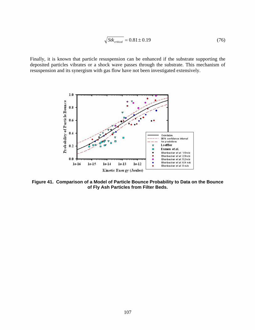
107
19.081.0 ±=criticalStk (76) Finally, it is known that particle resuspension can be enhanced if the substrate supporting the deposited particles vibrates or a shock wave passes through the substrate. This mechanism of resuspension and its synergism with gas flow have not been investigated extensively.
Figure 41. Comparison of a Model of Particle Bounce Probability to Data on the Bounce
of Fly Ash Particles from Filter Beds.

108

109
4. CONCLUSIONS
Conclusions that can be drawn from this review of the available information on aerosol transport through leak pathways are:
• The Morewitz-Vaughan correlation for leak pathway plugging does not provide a complete description of aerosol behavior in leaks. In fact, the correlation is applicable for only a narrow portion of the range of aerosol concentrations and particle sizes of interest for the analysis of reactor accidents.
• The criteria for sampling developed by Davies and by Agarwal and Liu are more
useful for assessing the susceptibility of leak pathways to plugging.
• There are abundant data available on the deposition of aerosol in idealizations of leak pathways. Data are available for capillaries, orifices, slots and cracks in concrete.
• Prediction of aerosol deposition is well developed for the conditions of laminar
flow through pathways with relatively smooth surfaces. Particle deposition is predominantly by diffusion of small particles and gravitational settling of larger particles.
• Prediction of aerosol transport in laminar flow through cracks in concrete is a
developing field.
• A robust base of data and models exists for predicting turbulent particle deposition in capillaries when surface roughness is not large.
• Under turbulent flow conditions aerosol deposition on surfaces may not be
permanent. Particles can bounce off surfaces they impact. Deposited particles can resuspend.
• There is a growing understanding of particle resuspension as a result of changes
in gas flow over deposits. Resuspension of deposited particles by particle impact and by shock or vibration is less well understood.
• It may be possible to model particle bounce from surfaces using a probabilistic
model based on the kinetic energy of the particle.

110

111
5. REFERENCES J.K. Agarwal and B.Y.H. Liu, “A criterion for accurate sampling in calm air”, American Industrial Hygiene Association Journal, 41 (1980) 191-197. A.W. Beeby, “The Prediction of Crack Widths in Hardened Concrete”, The Structural Engineer, 57A (1979) 9-17. L. Biasi, A. de los Reyes, M.W. Reeks, and G.F. de Santi, “Use of a simple model for the interpretation of experimental data on particle resuspension in turbulent flows”, J. Aerosol Science, 32 (2001) 1175-1200. R.B. Bird, W.E. Stewart and E.N. Lightfoot, Transport Phenomena, John Wiley and Sons, 1960. H. Boussa, C. Tognazzi-Lawrence, and C. La Borderie, “A model for computation of leakage through damaged concrete structures”, Cement and Concrete Composites, 23 (2001) 279-287. B.D. Bowen, S.Levin, and N. Epstein,”Fine particle depsoition in laminar flow through parallel-plate and cylindrical channels”, J. Colloid Interface Science, 54 (1976) 375-390. W.E. Browing, Jr. and R.D. Ackley, “Attenuation of Fission Product Escape by Intrinsic Properties, Nuclear Safety Program Semiannual Report, ORNL -3483, Oak Ridge National Laboratory, Oak Ridge, TN, September 13, 1963. A.C. Burton, J. P. Mitchell, and D.A.V. Morton, “The influence of pressure on the penetration of aerosol through fine capillaries, J. Aerosol Science, 24 (suppl. 1) (1993) 559-560. F.R. Carrié and M.P. Modera, “Particle Deposition in a Two-Dimensional Slot from a Transverse Stream”, Aerosol Science and Technology, 28 (1998) 235-246. F.R. Carrié and M.P. Modera, “Experimental investigation of aerosol deposition on slot and joint type leaks”, Journal of Aerosol Science, 33 (2002) 1447-1462. Y.K. Chen and C.P. Yu, “Particle deposition from duct flows by combined mechanisms”, Aerosol Science and Technology, 19 (1993) 389-395. B. Dahneke, “Particle Bounce or Capture - Search for an Adequate Theory: I. Conservation-of-Energy Model for a Simple Collision Process”, Aerosol Science and Technology, 23 (1995) 25-39. C.N. Davies, “The entry of aerosol into sampling tubes and heads”, British J. Applied Physics, Journal of Physics D, 1 (1968) 921-932. W. De Marcus and J.W. Thomas, Theory of the Diffusion Battery, ORNL-1413, Oak Ridge National Laboratory, Oak Ridge, TN, 1952.

112
S. Dunnet, “A Mathematical Study of the Sampling characteristics of a Thin-walled Sampler Operating in Calm Air”,Aerosol Science and Technology, 17 (1992) 93-104. K. Eleftheriadis and I. Colbeck, “The particle collection efficiency of rectangular strips by inertial impaction”, J. Aerosol Science, 23 (1992) S35-S38. M.J. Ellenbecker, D. Leith, and J.M Price, “Impaction and Particle Bounce at High Stokes Numbers”, Journal Air Pollution Control Association, 30 (1980) 1224-1227. M.S. El-Shobokshy, “Experimental Measurements of Aerosol Deposition to Smooth and Rough Surfaces”, Atmospheric Environment, 17 (1983) 639-644. N.A. Esmen, P. Ziegler, and R. Whitfield, “The adhesion of particles upon impaction”, J. Aerosol Science, 9 (1978) 547-556. L.J. Forney and L.A. Spielman, “Deposition of Course Aerosols from Turbulent Flows”, J. Aerosol Science, 5 (1974) 257-271. S.K. Friedlander and H.F. Johnstone, “Deposition of Suspended Particles from Turbulent Gas Streams”, Ind. Eng. Chem., 49 (1957) 1151-1156. T. Gelain and J. Vendel, “Research works on contamination transfers through cracked concrete walls”, Nuclear Engineering and Design, 238 (2008) 1159-1165. U. Greiner and W. Ramm, “Air leakage characteristics in cracked concrete”, Nuclear Engineering and Design, 156 (1995) 167-172. P.G. Gormley and M. Kennedy, “Diffusion from a stream flowing through a cylindrical tube”, Proc. Royal Irish Acad., 52-A (1949) 163-169. J.E. Haaland, “Simple and Explicit Formulas for the Friction Factor in Turbulent Flow”, J. Fluids Engineering, 103 (1983) 89-90 R.K. Hilliard and A.K. Postma, “Large-scale Fission Product Containment Tests”, Nuclear Technology, 53 (1981) 163-175. K. Hirao, T. Zama, M. Goto, Y. Naruse, K. Saito, T. Suzuki, and H. Sugino, “High-temperature leak-characteristics of PCV hatch flange gasket”, Nuclear Engineering and Design, 145 (1993) 375-386. K.H. Im and R.K. Ahluwalia, “Turbulent Eddy Deposition of Particles on Smooth and Rough Surfaces”, J. Aerosol Science, 20 (1989) 431-436. D.B. Ingham, “Diffusion of aerosols from a stream flowing through a cylindrical tube”, J. Aerosol Science, 6 (1975) 125-132.

113
W. John, “Particle-surface interactions: Charge transfer, Energy Loss, Resuspension and Deagglomeration”, Aerosol Science and Technology, 23 (1995) 2-24. W. John and V. Sethi, “Threshold for Resuspension by Particle Impaction”, Aerosol Science and Technology, 19 (1993) 69-79. O. Kuyama, Y. Kousaka, and K. Hyashi, “Change in Size Distribution of Ultrafine Aerosol Particles Undergoing Brownian Coagulation”, J. Colloid Interface Science, 101 (1984) 98-109. E.N. Landis, T. Zhang, E.N. Nagy, G. Nagy, and W.R. Franklin, “Cracking, damage and fracture in four dimesnions”, Materials and Structures, 40 (2007) 357-364. K.E. Lee and J.A. Gieseke, “Deposition of Particles in Turbulent Pipe Flows”, J. Aerosol Science, 25 (1994) 699. F. Leonhardt, “Crack Control in Concrete Structures” IABSESurveys, S-4/77, IABSE Periodica 3/1977, International Association for Bridge and Structural Engineering, Surich, August, 1977. S. Lewis, “Solid particle penetration into enclosures”, J. Hazardous Materials, 43 (1995) 195-216. B.Y. H. Liu and J.K. Agarwal, “Experimental Observation of Aerosol Deposition in Turbulent Flow”, J. Aerosol Science, 5 (1974) 145-155. D-L.Liu and W.W. Nazaroff, “Modeling Pollutant Penetration Across Building Envelopes”, Atmos. Environm., 35 (2001) 4451-4462. D-L. Liu and W.W. Nazaroff, “Particle Penetration Through Building Cracks”, Aerosol Science and Technology, 37 (2003) 565-573. F. Löffler, “Adhesion probability in fibre filters”, Clean Air, 8 (1974) 75. A.R. McFarland, H. Gong, A. Muyshondt, W.B Wente, and N.K. Anand, “Aerosol Deposition in Bends with turbulent Flow”, Environmental Science and Technology, 31 (1997) 3371-3377. J.P. Mitchell, R.T. Edwards, and M.A.E. Ball, “The penetration of aerosols through fine capillaries”, RAMTRANS, Volume 1 (no.3) (1990) 101-106. J.P. Mitchell, I.A. Marshall, L.J. Latham and M.H.E. Ball, “The Penetration of Aerosols Through Fine Orifices”, RAMTRANS, 3 (1992) 5-17. T.L. Montgomery and M. Corn, “Aerosol Deposition in a Pipe with Turbulent Air Flow”, J. Aerosol Science, 1 (1970) 185-213.

114
H.A. Morewitz, R.P. Johnson, C.T. Nelson, E.U. Vaughan, C.A. Guderjahn, R.K. Hilliard, J.D. McCormack, and A.K. Postma, “Attenuation of Airborne Debris from Liquid-metal Fast Breeder Reactor Accidents”, Nuclear Technology, 46 (1979) 332-339. H.A. Morewitz, “Leakage of Aerosol from Containment Buildings”, Health Physics, 42 (1982) 195-207. D.A.V. Morton and J.P. Mitchell, “Aerosol Penetration Through Capillaries and Leaks: Experimental Studies on the Influence of Pressure”, J. Aerosol Science, 26 (1995) 353-367; additional information is available apparently in A.C. Burton, C. Clement, J.P. Mitchell, and D.A.V. Morton, “The influence of aerosol concentration and pressure on the penetration of aerosols through fine capillaries”, AEA Technology Report AEA-EE-0485, AEA Technology, Winfrith, UK. It has not been possible to retrieve this laboratory report. R.B. Mosely, D.J. Greenwell, L.E. Sparks, Z. Guo, W.G.Tucker, R.Fortmann, C. Whitfield, “Penetration of Ambient Fine Particles into the Indoor Environment”, Aerosol Science and Technology, 34 (2001) 127-136. A. Muyshondt, N.K. Anand, and A.R. McFarland, “Turbulent Deposition of Aerosol Particles in Large Transport Tests”, Aerosol Science and Technology, 24 (1996) 107-116. C.T. Nelson and R.P. Johnson, “Aerosol Leakage Tests”, Status of Safety Technology for Radiological Consequences of Postulated Accidents in Liquid Metal Fast Breeder Reactors, Energy Resources and Development Administration, ERDA-56, 1975. V.J. Novick, “Plugging Passages with Particles: Refining the Morewitz Criteria”, Aerosol Science and Tech., 21 (1994) 219-222. P.C. Owzarski, S.L. Sutter, L.C. Schwendiman, J. Mishima, and T.J. Bander, Measured and Predicted Gas Flow Rates Through Rough Capillaries, NUREG/CR0745, PNL-2623, Pacific Northwest Laboratory, Richland, WA, June 1979. Y.C. Pan, A.H. Marchertas and J.M. Kennedy, “Failure/Leakage Predictions of Concrete Structures Containing Cracks”, p. 247-256 in Proceedings of the Second Workshop on Containment Integrity, NUREG/CP-0056; SAND84-1514, T. Molina and R. Cochrell, editors, Sandia National Laboratories, Albuquerque, NM, August 1984. P.G. Papavergos and A.B. Hedley, “Particle deposition behaviour from turbulent flows”, Chemical engineering Research and Design, 62 (1984) 275-295. S. Parker, T. Foat, S. Preston, “Towards quantitative prediction of aerosol deposition from Turbulent flows”, J. Aerosol Science, 39 (2008) 99-112. F. Parozzi, et al., “Investigation on Aerosol Transport in Containment Cracks”, International Conference on Nuclear Energy for New Europe 2005, Bled, Slovenia, September 5-8, 2005
115
J. Pich, “Theories of gravitational deposition of particles from laminar flows in channels”, J. Aerosol Science, 3 (1972) 351-361. A.K. Postma and L.C. Schwendiman, Studies in Micrometrics. I. Particle Depopsition in Conduits as a Source of Arror in Aerosol Sampling, HW-65308, Hanford Atomic Products Operation, Richland WA, may 12, 1960. M.W. Reeks and D. Hall, “Kinetic models for particle resuspension in turbulent flows: Theory and measurement”, J. Aerosol Science, 32 (2001) 1-31. H.E. Regtuit, C.J. De Ruiter, E.L.M. Vrins, P. Hofschreuder, F. Oeseburg, and F.M Benschop, “The tunnel impactor. A multiple inertial impactor for coarse aerosol”, J. Aerosol Science, 21 (1990) 919-933. R. Riva, L. Brusa, P. Contri, and L. Imperato, “Prediction of air and steam leak rate through cracked reinforced concrete panels”, Nuclear Engineering and Design, 192 (1999) 13-30. S.H. Rizkalla, B.L. Lau, and S. H. Simmonds, “Air Leakage Characteristics in Reinforce Concrete”, J. Structural Engineering, 110 (1984)1149-1162. Somewhat similar information was published in S.H. Rizkalla, B.L. Lau, and S.H. Simmonds, “Leakage of Pressurized Gases Through Unlined Concrete Containment Structures”, Transactions of the 7th International Conference on Structural Mechanics in Reactor Technology, North-Holland Physics Publishing, Amsterdam, 1983. Rockwell International, Annual Technical Progress Report LMFBR Safety Program Government Fiscal Year 1977, AI-DOE-13210, December 1977. E. Schlangen and E.J. Garboczi, “New method of simulating fracture using an elastically uniform random geometry lattice”, International Journal of Engineering Science, 34 (1996) 1131-1141. L.C.Schwendiman and S.L. Sutter, Transport of Particles Through Gas Leaks - A Review, BNWL-2218, Pacific Northwest Laboratory, Richaland WA, January 1977 G.A. Sehmel, “Particle Deposition from Turbulent Air Flow”, J. Geophysical Research, 75 (1970) 1766-1781. M. Shimada, K. Okuyama, and M. Asai, “Deposition of Submicron Aerosol Particles in Turbulent and Transition Flow”, AIChE J., 39 (1993) 17-26. D. Sinclair, R.J. Countess, B.Y.H. Liu, and D.H.H. Pui, Experimental Verification of Diffusion Battery Theory”, Air Pollution Control Association Journal, 26 (1976) 661-663. M.R. Sippola and W.W. Nazaroff, Particle Deposition from Turublent Flow: Review of Published Research and Its Applicability to Ventilation Ducts in Commercial Buildings, LBNL-51432, Lawrence Berkeley National Laboratory Report, June 2002.

116
M. Stegemann, B. Masson, L. Coudert, J-P. Touret, N. Herrmann, and L. Stempniewski, “Experimental Investigation of the Leakage Behaviour of Reinforced Concrete Walls”, 18th International Conference on Structural Mechanics in Reactor Technology (SmiRT 18), Beijing, China, August 7-12, 2005. S.L. Sutter, J.W. Johnston, J. Mishima, P.E. Owzarski, L.C. Schwendiman, and G.B. Long, Depleted Uranium Dioxide Powder Flow Through Very Small Openings, NUREG/CR-1099, PNL-3177, Pacific Northwest Laboratory, Richland, WA., February 1980. A.S.W. Thomas and K.C. Cornelius, “Investigation of Laminar Boundary-layer Suction Slot”, AIAA Journal, 20 (1982)790-796 C. Thornton, K.K. Yin, and M.J. Adams, “Numerical simulation of the impact fracture and framentation of agglomerates”, J. Phys. D. Appl. Phys., 29 (1996) 424-435. C.J. Tsai, D.Y. Pui, and B.Y.H. Liu, “Capture and Rebound of Small Particles Upon Impact with Solid Surfaces”, Aerosol Science and Technology, 12 (1990) 497-507. J.F. van de Vate, “Safety Containment Buildings as Barriers Against Particulate Radioactivity Release under Accident Conditions”, Nuclear Technology, 81 (1988) 246-256. E.U. Vaughan, “Simple Model of Plugging of Ducts by Aerosol Deposits”, Trans. ANS, 22 (1978 ) 507. A. Watanabe, T. Hashimoto, and M. Osake, “Fission Product Aerosol Trapping Effects in the Leakage Path of Containment Penetrations Under Severe Accident Conditions”, NUPEC, unpublished. A.C. Wells and A.C. Chamberlain, “Transport of small particles to vertical surfaces”, British J. Appl. Physics, 18 (1967) 1793-1799. M.M.R. Williams, “Particle Deposition and Plugging in Tubes and Cracks (with Special Reference to Fission Product Retention)”, Progress in Nuclear Energy, 28 (1994) 1-60. M. Xu, K. Willeke, P. Biswas, and S.I. Pratsinis, “Impact and Rebound of Particles at Acute Incident Angles”, Aerosol Science and Technology, 18 (1993) 143-155. H. Yoshida, M. Uragami, H. Masuda, and K. Iinoya, Kagaku Kogaku Ronbunshu, 4 (1979) 123-128. C.P. Yu, C.S. Liu, and D.B. Taulbee, “Simultaneous diffusion and sedimentation of aerosols in a horizontal cylinder ”, J. Aerosol Science, 8 (1977)309-316.

117
APPENDIX A: DERIVATION OF THE STOKES NUMBER
Consider an aerosol particle suspended in a quiescent gas medium and subject to gravitational force. The steady state gravitational settling velocity of the aerosol particle is given by a balance between the gravitational force on the particle and the drag force on the particle:
( )B
VV
CDCgD settling
settlingslip
pgDgmp ==− 223
421
6χπρρρπ (77)
where
B - particle mobility (s/g) DC - drag coefficient (-)
slipC - slip correction factor (-)
pD - diameter of a sphere with the same mass as the particle in question (cm) g - gravitational acceleration (980.665 cm/s2)
gρ - gas density (g/cm3)
mρ - density of the material making up the aerosol particle (g/cm3)
settlingV - settling velocity (cm/s) χ - dynamic shape factor (-)
For perfectly spherical, fully dense particles, the shape factor, χ, is equal to one. For all real aerosol particles, the shape factor is greater than one. For the particles of interest here, the slip correction factor, Cslip, differs little from unity. For the Stokes regime (Rep < 1), the drag coefficient is given by:
p
DCRe24
= (78)
g
settlinggpp
VDµ
ρ=Re (79)
where
pRe - particle Reynolds number (-)
gµ - gas viscosity (g/cm-s)

118
For larger particles and higher velocities such that the particle Reynolds number exceeds unity, the drag coefficient is given by more complicated expressions involving the Reynolds number. For algebraic simplicity it will be assumed for the purposes of this derivation that only the Stokes regime is of interest. For detailed calculations, more careful attention will have to be devoted to the drag coefficient. Then,
( ) settlingslip
pggmp V
CD
gDχπµ
ρρπ 36
3 =− (80)
χµρ
g
mpslipsettling
gDCV
18
2
= (81)
χπµ pg
slip
DC
B3
= (82)
From the Stokes-Einstein relationship and the particle mobility, the aerosol particle diffusion coefficient can be determined:
χπµ pg
slip
DkTC
D3
= (83)
where
D - aerosol particle diffusion Reynolds number (-) The mobility conveniently relates the particle velocity to the force on the particle. Consider now the same particle subjected to a gas velocity U∞. The differential equation for the particle velocity, V, is:
B
VUdtdVD mp
−=
∞
ρπ 3
6 (84)
or
slippm
g
CDdtdV
VU 2
1811ρ
χµτ==
−∞ (85)

119
where
t - time (s) τ - particle relaxation time (s) V - particle velocity (cm/s)
The particle relaxation time divided by the life time of turbulent eddies yields a dimensionless time that is useful for the correlation of turbulent deposition of aerosol particles. The particle relaxation time multiplied by the gas velocity yields a characteristic distance of particle travel: ∞= Ud τ (86) This characteristic distance of particle travel can be compared to characteristic dimensions of the flow path for the particle. A plausible characteristic distance for flow in a cylindrical leak is the leak radius, Dcyl/2. The ratio of the particle characteristic travel distance and the characteristic dimension of the apparatus yields the dimensionless quantity called the Stokes number:
cylg
slippm
cylcyl DUCD
DU
DdStk
χµρτ
922 2 ∞∞
=== (87)
Note that some prefer to use the cylinder diameter rather than the cylinder radius as the characteristic dimension of the flow path. The Stokes number is often used for the correlation of particle deposition data due to inertial impaction. Seldom is it the only correlating variable.

120
121
APPENDIX B: TABULATED DATA ON TURBULENT DEPOSITION OF
AEROSOL PARTICLES IN SMOOTH TUBES
Tabulated data on the dimensionless deposition velocity, , as a function of dimensionless particle relaxation time, , as defined in the text, are provided for experimental investigations discussed in the text.

122
Tabl
e B
-1.
Tabl
ulat
ed D
ata
from
Inve
stig
atio
ns b
y Fo
rney
and
Spi
elm
an U
sing
Tub
es C
oate
d w
ith a
Mix
ture
of 7
5% P
araf
fin
Oil
and
25%
Pet
role
um J
elly
to S
uppr
ess
Part
icle
Bou
nce.
d p =
30.
9 µm
D
pipe
= 1
.30
cm
d p =
30.
9 µm
D
pipe
= 1
.78
cm
d p =
30.
9 µm
D
pipe
= 2
.54
cm
d p =
19.
0 µm
D
pipe
= 1
.30
cm
d p =
19.
0 µm
D
pipe
= 1
.78
cm
d p =
19.
0 µm
D
pipe
= 2
.54
cm
147
0.15
3 27
.6
0.21
7 28
.0
0.17
8 10
1
0.23
0
98.6
0.
406
58
.8
0.13
9 14
7 0.
205
27.6
0.
342
35.9
0.
267
101
0.
120
98
.6
0.32
1
58.8
0.
126
217
0.19
6 27
.6
0.25
3 59
.4
0.17
6 10
1
0.23
9
58.8
0.
139
58
.8
0.19
5 21
7 0.
264
27.6
0.
211
59.4
0.
158
101
0.
0777
58
.8
0.12
6
58.8
0.
149
217
0.36
2 67
.3
0.25
0 12
0.8
0.21
6 21
5
0.29
2
58.8
0.
195
86
.9
0.20
7 34
5 0.
143
67.3
0.
318
200
0.25
3 21
5
0.30
4
86.9
0.
252
345
0.18
2 67
.3
0.36
5 20
0 0.
242
23.7
0.
177
67.3
0.
417
3.56
0.
0267
23
.7
0.11
1
10
7 0.
226
4.89
0.
113
23.7
0.
110
107
0.39
2 7.
13
0.17
3
10
7 0.
385
11.9
0.
152
107
0.29
0 17
.1
0.20
1
22
6
0.21
8
26.9
0.
188
226
0.
240
36
.3
0.26
1
33
5
0.22
4
60.8
0.
159
335
0.
279
60
.8
0.17
2
59
.6
0.19
5
12
2 0.
177
122
0.21
3
20
0 0.
239
196
0.26
5
29
2 0.
283
Not
e: D
ata
wer
e ob
tain
ed b
y di
gitiz
ing
a sm
all g
raph
.
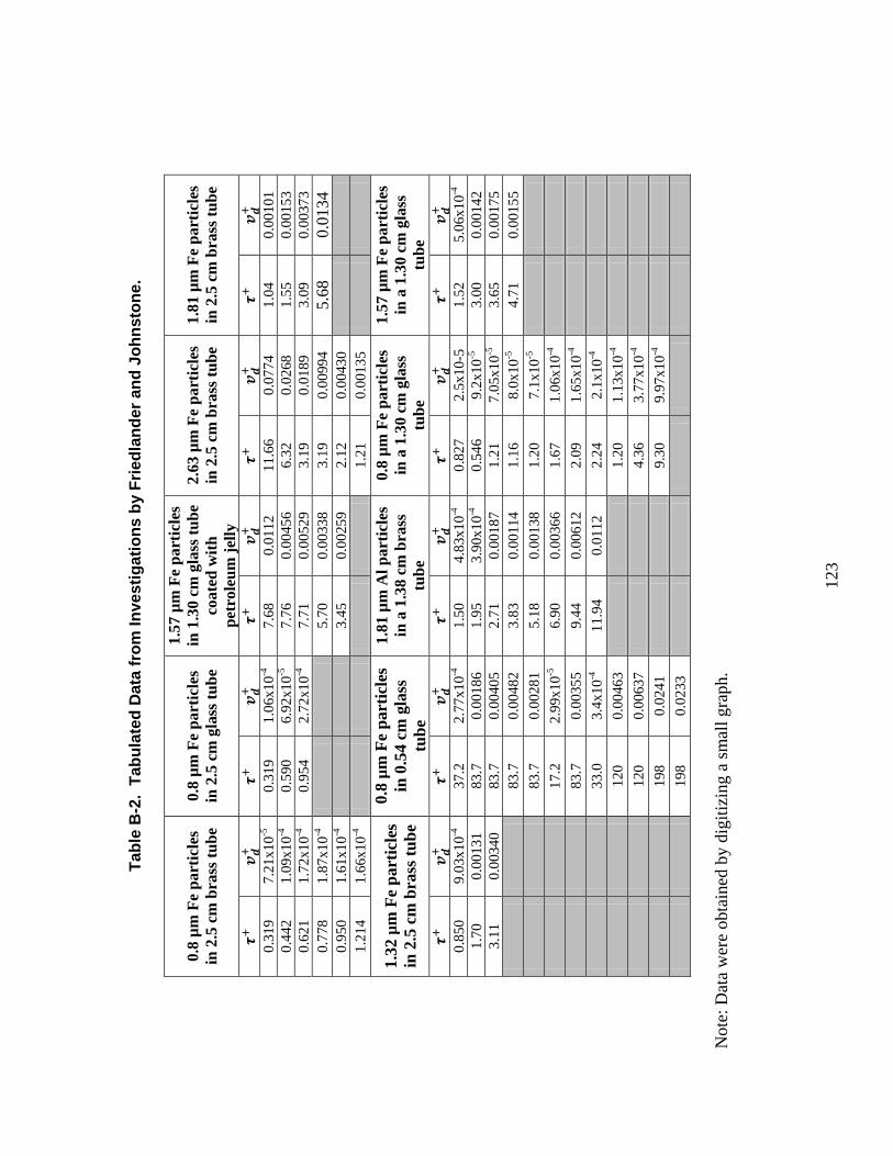
123
Ta
ble
B-2
. Ta
bula
ted
Dat
a fr
om In
vest
igat
ions
by
Frie
dlan
der a
nd J
ohns
tone
.
0.8
µm F
e pa
rtic
les
in 2
.5 c
m b
rass
tube
0.
8 µm
Fe
part
icle
s in
2.5
cm
gla
ss tu
be
1.57
µm
Fe
part
icle
s in
1.3
0 cm
gla
ss tu
be
coat
ed w
ith
petr
oleu
m je
lly
2.63
µm
Fe
part
icle
s in
2.5
cm
bra
ss tu
be
1.81
µm
Fe
part
icle
s in
2.5
cm
bra
ss tu
be
0.31
9 7.
21x1
0-5
0.31
9 1.
06x1
0-4
7.68
0.
0112
11
.66
0.07
74
1.04
0.
0010
1 0.
442
1.09
x10-4
0.
590
6.92
x10-5
7.
76
0.00
456
6.32
0.
0268
1.
55
0.00
153
0.62
1 1.
72x1
0-4
0.95
4 2.
72x1
0-4
7.71
0.
0052
9 3.
19
0.01
89
3.09
0.
0037
3 0.
778
1.87
x10-4
5.
70
0.00
338
3.19
0.
0099
4 5.
68
0.01
34
0.95
0 1.
61x1
0-4
3.45
0.
0025
9 2.
12
0.00
430
1.21
4 1.
66x1
0-4
1.21
0.
0013
5
1.32
µm
Fe
part
icle
s in
2.5
cm
bra
ss tu
be
0.8
µm F
e pa
rtic
les
in 0
.54
cm g
lass
tu
be
1.81
µm
Al p
artic
les
in a
1.3
8 cm
bra
ss
tube
0.8
µm F
e pa
rtic
les
in a
1.3
0 cm
gla
ss
tube
1.57
µm
Fe
part
icle
s in
a 1
.30
cm g
lass
tu
be
0.85
0 9.
03x1
0-4
37.2
2.
77x1
0-4
1.50
4.
83x1
0-4
0.82
7 2.
5x10
-5
1.52
5.
06x1
0-4
1.70
0.
0013
1 83
.7
0.00
186
1.95
3.
90x1
0-4
0.54
6 9.
2x10
-5
3.00
0.
0014
2 3.
11
0.00
340
83.7
0.
0040
5 2.
71
0.00
187
1.21
7.
05x1
0-5
3.65
0.
0017
5
83
.7
0.00
482
3.83
0.
0011
4 1.
16
8.0x
10-5
4.
71
0.00
155
83.7
0.
0028
1 5.
18
0.00
138
1.20
7.
1x10
-5
17.2
2.
99x1
0-5
6.90
0.
0036
6 1.
67
1.06
x10-4
83
.7
0.00
355
9.44
0.
0061
2 2.
09
1.65
x10-4
33
.0
3.4x
10-4
11
.94
0.01
12
2.24
2.
1x10
-4
120
0.00
463
1.20
1.
13x1
0-4
120
0.00
637
4.36
3.
77x1
0-4
198
0.02
41
9.30
9.
97x1
0-4
198
0.02
33
Not
e: D
ata
wer
e ob
tain
ed b
y di
gitiz
ing
a sm
all g
raph
.
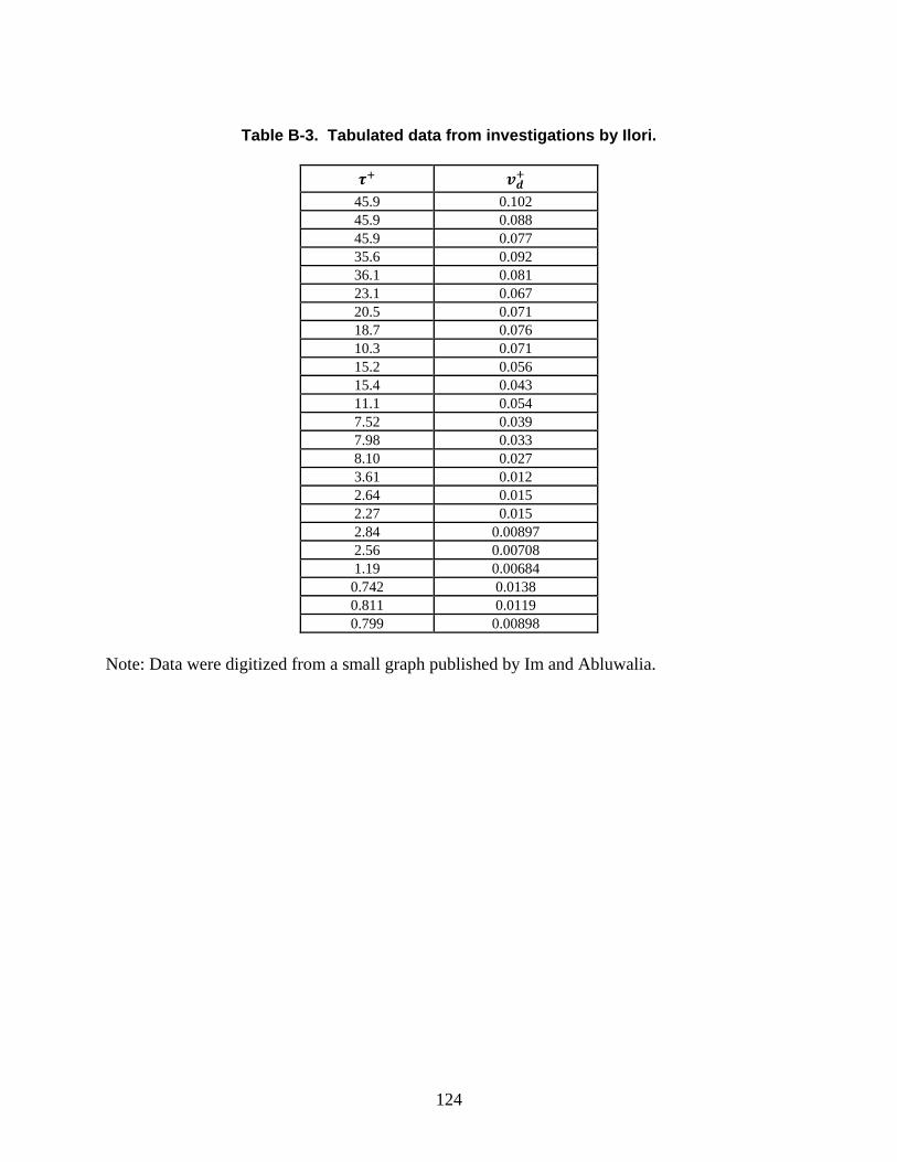
124
Table B-3. Tabulated data from investigations by Ilori.
45.9 0.102 45.9 0.088 45.9 0.077 35.6 0.092 36.1 0.081 23.1 0.067 20.5 0.071 18.7 0.076 10.3 0.071 15.2 0.056 15.4 0.043 11.1 0.054 7.52 0.039 7.98 0.033 8.10 0.027 3.61 0.012 2.64 0.015 2.27 0.015 2.84 0.00897 2.56 0.00708 1.19 0.00684 0.742 0.0138 0.811 0.0119 0.799 0.00898
Note: Data were digitized from a small graph published by Im and Abluwalia.
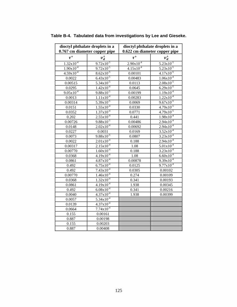
125
Table B-4. Tabulated data from investigations by Lee and Gieseke.
dioctyl phthalate droplets in a 0.767 cm diameter copper pipe
dioctyl phthalate droplets in a 0.622 cm diameter copper pipe
1.32x10⁻⁴ 9.72x10⁻⁵ 2.90x10⁻⁴ 5.23x10⁻⁵ 1.90x10⁻⁴ 9.72x10⁻⁵ 4.15x10⁻⁴ 5.23x10⁻⁵ 4.59x10⁻⁴ 8.62x10⁻⁵ 0.00101 4.17x10⁻⁵
0.0022 6.43x10⁻⁵ 0.00483 1.06x10⁻⁴ 0.00515 5.34x10⁻⁵ 0.0113 2.08x10⁻⁵ 0.0295 1.42x10⁻⁴ 0.0645 6.29x10⁻⁵
9.05x10⁻⁴ 9.88x10⁻⁵ 0.00199 1.19x10⁻⁴ 0.0013 1.11x10⁻⁴ 0.00283 1.22x10⁻⁴
0.00314 5.39x10⁻⁵ 0.0069 9.67x10⁻⁵ 0.0151 1.55x10⁻⁴ 0.0330 4.79x10⁻⁵ 0.0352 1.37x10⁻⁴ 0.0771 4.79x10⁻⁵ 0.202 2.55x10⁻⁴ 0.441 1.98x10⁻⁴
0.00726 9.88x10⁻⁵ 0.00486 2.94x10⁻⁴ 0.0148 2.02x10⁻⁴ 0.00692 2.94x10⁻⁴ 0.0227 0.0031 0.0169 3.52x10⁻⁴ 0.0073 9.88x10⁻⁵ 0.0807 3.23x10⁻⁴ 0.0022 2.01x10⁻⁴ 0.188 2.94x10⁻⁴
0.00317 2.15x10⁻⁴ 1.08 5.01x10⁻⁴ 0.00770 1.60x10⁻⁴ 0.188 3.23x10⁻⁴ 0.0368 4.19x10⁻⁴ 1.08 6.60x10⁻⁴ 0.0861 4.87x10⁻⁴ 0.00878 9.39x10⁻⁴ 0.492 6.75x10⁻⁴ 0.0125 9.77x10⁻⁴ 0.492 7.43x10⁻⁴ 0.0305 0.00102
0.00770 1.46x10⁻⁴ 0.274 0.00109 0.0368 1.32x10⁻⁴ 0.341 0.00193 0.0861 4.19x10⁻⁴ 1.938 0.00345 0.492 6.08x10⁻⁴ 0.341 0.00216
0.0040 4.37x10⁻⁴ 1.938 0.00399 0.0057 5.34x10⁻⁴ 0.0139 4.37x10⁻⁴ 0.0664 7.74x10⁻⁴ 0.155 0.00161 0.887 0.00198 0.155 0.00203 0.887 0.00408
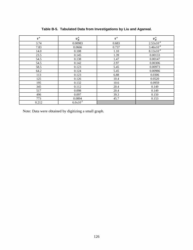
126
Table B-5. Tabulated Data from Investigations by Liu and Agarwal.
3.74 0.00983 0.683 2.53x10⁻⁴ 7.83 0.0666 0.737 3.46x10⁻⁴ 14.0 0.108 1.10 8.13x10⁻⁴ 23.5 0.145 1.39 0.00133 54.5 0.138 1.47 0.00147 54.5 0.142 2.97 0.00306 58.5 0.123 5.45 0.00973 64.2 0.124 5.45 0.00986 113 0.123 6.88 0.0306 125 0.126 10.4 0.0520 195 0.132 10.6 0.0959 345 0.112 20.4 0.149 517 0.098 20.4 0.149 496 0.097 39.3 0.150 773 0.0894 45.7 0.153
0.212 6.0x10⁻⁵ Note: Data were obtained by digitizing a small graph.

127
Table B-6. Tabulated Data from Investigations by Montgomery and Corn.
1.60 0.0385 1.10 0.00177 1.14 9.05x10⁻⁴
0.0257 8.12x10⁻⁴ 0.871 0.00965 0.399 5.96x10⁻⁴
0.0730 4.79x10⁻⁴ 0.0209 1.78x10⁻⁴ 0.115 4.67x10⁻⁵ 2.88 0.00506
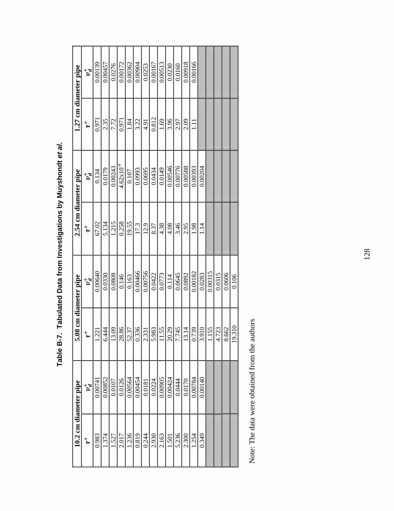
128
Ta
ble
B-7
. Ta
bula
ted
Dat
a fr
om In
vest
igat
ions
by
Muy
shon
dt e
t al.
10
.2 c
m d
iam
eter
pip
e 5.
08 c
m d
iam
eter
pip
e 2.
54 c
m d
iam
eter
pip
e 1.
27 c
m d
iam
eter
pip
e
0.
983
0.00
741
1.22
1 0.
0064
0 67
.02
0.13
4 0.
971
0.00
139
1.37
4 0.
0085
2 6.
444
0.03
30
5.13
4 0.
0179
2.
35
0.00
457
1.52
7 0.
0107
13
.09
0.08
08
1.21
5 0.
0024
3 7.
72
0.02
76
2.01
7 0.
0126
28
.86
0.14
6 0.
258
4.62
x10-4
0.
971
0.00
172
1.23
6 0.
0056
4 52
.37
0.16
3 19
.55
0.10
7 1.
84
0.00
362
0.81
9 0.
0045
4 0.
336
0.00
466
17.3
0.
0993
3.
22
0.00
904
0.24
4 0.
0181
2.
331
0.00
756
12.9
0.
0695
4.
91
0.02
53
2.93
0 0.
0224
5.
983
0.04
22
8.37
0.
0434
0.
812
0.00
167
2.16
3 0.
0090
5 11
.55
0.07
73
4.38
0.
0149
1.
69
0.00
513
1.50
1 0.
0042
4 20
.29
0.11
4 4.
08
0.00
546
3.96
0.
0230
5.
236
0.04
44
7.74
5 0.
0645
3.
46
0.00
776
2.97
0.
0160
2.
300
0.01
70
13.1
4 0.
0892
2.
95
0.00
588
2.09
0.
0091
8 1.
254
0.00
784
0.73
9 0.
0018
2 1.
98
0.00
393
1.11
0.
0016
6 0.
349
0.00
140
3.91
0 0.
0283
1.
14
0.00
204
1.15
5 0.
0031
5
4.
723
0.03
15
8.66
2 0.
0606
19
.310
0.
106
Not
e: T
he d
ata
wer
e ob
tain
ed fr
om th
e au
thor
s
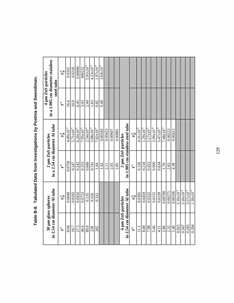
129
Ta
ble
B-8
. Ta
bula
ted
Dat
a fr
om In
vest
igat
ions
by
Post
ma
and
Swen
dim
an.
30 µ
m g
lass
sphe
res
in 2
.54
cm d
iam
eter
Al t
ube
2 µm
ZnS
par
ticle
s in
a 2
.54
cm d
iam
eter
Al t
ube
4 µm
ZnS
par
ticle
s in
a 1
.905
cm
dia
met
er st
ainl
ess
stee
l tub
e
8.
04
0.00
49
0.07
50
4.49
x10-5
16
.6
0.03
52
16.7
0.
0192
0.
147
5.71
x10-5
10
.0
0.02
18
27.3
0.
0410
0.
242
6.20
x10-5
6.
45
0.00
696
46.6
0.
0723
0.
353
7.95
x10-5
3.
43
0002
32
89.8
0.
135
0.60
0 2.
54x1
0-4
2.44
5.
91x1
0-4
228
0.31
6 0.
741
5.98
x10-4
1.
63
4.23
x10-4
26
5 0.
333
1.04
7.
82x1
0-4
0.82
1.
07x1
0-4
1.42
0.
0018
3 0.
49
3.64
x10-5
2.
11
0.00
423
2.05
0.
0060
7
2.
85
0.00
881
4 µm
ZnS
par
ticle
s in
2.5
4 cm
dia
met
er A
l tub
e 2
µm Z
nS p
artic
les
in 1
.905
cm
stai
nles
s ste
el tu
be
11.1
0.
0395
0.
126
4.31
x10-6
8.
08
0.04
59
0.21
8 1.
29x1
0-5
7.98
0.
0322
0.
423
5.17
x10-5
5.
46
0.01
55
0.90
0 2.
99x1
0-4
4.11
0.
0139
0.
634
5.47
x10-5
2.
86
0.00
708
1.70
7.
48x1
0-4
2.32
0.
0027
5 2.
63
0.00
223
1.40
0.
0010
6 4.
38
0.00
413
0.92
5 3.
39x1
0-4
0.56
7 3.
16x1
0-4
0.28
5 3.
57x1
0-4
0.28
4 1.
30x1
0-4

130
Ta
ble
B-9
. Ta
bula
ted
Dat
a fr
om In
vest
igat
ions
by
Shim
ada,
Oka
yam
a, a
nd A
sai.
0.
043
µm N
aCl p
artic
les
Csl
ip =
5.8
4 0.
021
µm N
aCl p
artic
les
Csl
ip =
11.
4 0.
017
µm N
aCl p
artic
les
Csl
ip =
13.
9 0.
01 µ
m N
aCl p
artic
les
Csl
ip =
23.
3
0.
0017
6 1.
92x1
0-6
0.00
105
4.38
x10-6
0.
0125
9.
62x1
0-6
0.00
563
2.16
x10-5
0.
0045
4 2.
36x1
0-6
0.00
154
5.74
x10-6
0.
0055
8 7.
96x1
0-6
0.00
583
1.70
x10-5
0.
0086
0 2.
56x1
0-6
0.00
158
6.89
x10-6
0.
0040
5 7.
79x1
0-6
0.00
557
1.60
x10-5
0.
0154
2.
68x1
0-5
0.00
194
4.22
x10-6
0.
0025
3 9.
41x1
0-6
8.97
x10-4
1.
45x1
0-5
0.02
40
2.58
x10-6
0.
0028
9 3.
86x1
0-6
0.00
184
9.70
x10-6
7.
23x1
0-4
1.10
x10-5
0.
0243
3.
20x1
0-6
0.00
359
4.94
x10-6
0.
0013
4 6.
44x1
0-6
0.04
71
2.65
x10-6
0.
0073
7 5.
05x1
0-6
0.00
535
7.05
x10-6
0.
0079
7 8.
40x1
0-6
0.01
19
5.86
x10-6
N
ote:
Dat
a w
ere
obta
ined
by
digi
tizin
g sm
all g
raph
s.

131
Table B-10. Tabulated Data from Investigations by Shobokshy.
0.435 1.01x10⁻⁴ 0.436 1.84x10⁻⁴ 0.923 3.95x10⁻⁴ 0.944 6.52x10⁻⁴ 1.63 8.80x10⁻⁴ 3.31 0.00213 3.06 0.00312 3.33 0.00558 4.51 0.00724 4.70 0.0110 4.51 0.0110 7.21 0.0289 7.22 0.0478 12.0 0.163 1.67 0.00140
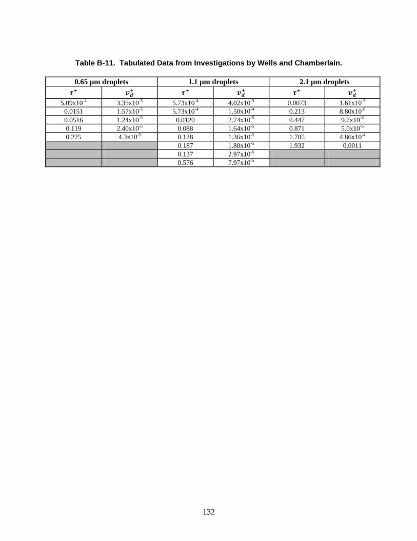
132
Table B-11. Tabulated Data from Investigations by Wells and Chamberlain.
0.65 µm droplets 1.1 µm droplets 2.1 µm droplets
5.09x10⁻⁴ 3.35x10⁻⁵ 5.73x10⁻⁴ 4.02x10⁻⁵ 0.0073 1.61x10⁻⁵ 0.0151 1.57x10⁻⁵ 5.73x10⁻⁴ 1.50x10⁻⁴ 0.213 8.80x10⁻⁶ 0.0516 1.24x10⁻⁵ 0.0120 2.74x10⁻⁵ 0.447 9.7x10⁻⁶ 0.119 2.40x10⁻⁵ 0.088 1.64x10⁻⁵ 0.871 5.0x10⁻⁵ 0.225 4.3x10⁻⁵ 0.128 1.36x10⁻⁵ 1.785 4.86x10⁻⁴
0.187 1.80x10⁻⁵ 1.932 0.0011 0.137 2.97x10⁻⁵ 0.576 7.97x10⁻⁵

133
Table B-12. Tabulated Data from Investigations by Sehmel.
0.533 cm tube 1.26 2.80x10⁻⁵ 0.398 5.28x10⁻⁵ 4.62 0.0031 1.73 1.22x10⁻⁴ 2.09 1.80x10⁻⁵ 1.84 9.61x10⁻⁴ 3.76 6.09x10⁻⁴ 2.01 3.38x10⁻⁵ 3.94 0.00321 3.78 7.97x10⁻⁴ 4.18 2.07x10⁻⁴ 11.0 0.00752 3.17 0.00105 4.09 4.59x10⁻⁴ 10.2 0.0193 3.16 0.00430 4.09 7.11x10⁻⁴ 10.8 0.0571 4.89 0.00386 9.14 0.0051 10.5 0.0618 11.4 0.104 15.3 0.0029 0.647 1.19x10⁻⁵ 1.575 cm tube 15.2 0.0032 0.514 5.88x10⁻⁵ 9.15 0.00509 1.16 5.99x10⁻⁶ 4.00 7.55x10⁻⁵ 12.1 0.00933 1.08 8.78x10⁻⁶ 3.98 3.36x10⁻⁴ 12.1 0.0120 1.18 1.12x10⁻⁵ 5.36 0.00346 12.2 0.0132 1.16 2.08x10⁻⁵ 6.74 0.00902 19.7 0.0689 1.10 5.45x10⁻⁵ 10.0 0.0331 22.5 0.0697 13.1 0.0905 14.7 0.0505 29.7 0.0602 21.1 0.0961 3.66 1.08x10⁻⁵ 0.484 2.52x10⁻⁶ 3.66 4.58x10⁻⁴
0.0754 2.61x10⁻⁵ 0.428 4.06x10⁻⁶ 3.63 5.40x10⁻⁴ 0.0749 3.31x10⁻⁵ 0.871 8.70x10⁻⁶ 3.63 8.66x10⁻⁴ 0.469 3.99x10⁻⁵ 0.450 1.32x10⁻⁵ 6.10 4.85x10⁻⁴ 1.31 5.59x10⁻⁵ 0.0895 3.48x10⁻⁵ 6.10 0.0012 1.30 2.26x10⁻⁴ 0.901 2.51x10⁻⁵ 6.10 0.0016 3.06 0.0400 0.876 3.24x10⁻⁵ 6.10 0.0018 3.06 0.0462 0.902 3.50x10⁻⁵ 9.06 0.0029
Note: Data obtained by digitizing small graphs.

134
Table B-12, Continued.
1.575 cm tube 7.75 0.0164 0.00195 1.44x10⁻⁵ 9.06 0.0040 8.75 0.0262 0.00195 1.60x10⁻⁵ 9.02 0.0050 8.76 0.0301 0.00161 2.66x10⁻⁵ 9.02 0.0080 9.56 0.087 0.00162 2.95x10⁻⁵ 8.98 0.0082 10.9 0.0706 0.040 7.79x10⁻⁶ 10.4 0.0076 15.2 0.0948 0.040 8.57x10⁻⁶ 10.4 0.0123 18.3 0.121 0.035 4.66x10⁻⁵ 14.5 0.0245 0.138 4.33x10⁻⁶ 0.398 7.25x10⁻⁶ 14.7 0.104 0.138 6.87x10⁻⁶ 0.398 7.95x10⁻⁶ 20.4 0.110 0.136 1.16x10⁻⁵ 0.398 4.97x10⁻⁶ 36.2 0.126 0.136 1.52x10⁻⁵ 0.172 7.55x10⁻⁶ 36.2 0.137 0.616 7.29x10⁻⁶ 1.59 3.49x10⁻⁵ 36.1 0.144 0.616 1.18x10⁻⁵ 1.59 5.28x10⁻⁵ 28.2 0.126 0.617 1.67x10⁻⁵ 1.59 1.56x10⁻⁴
0.0275 4.87x10⁻⁶ 0.617 2.50x10⁻⁵ 1.60 2.61x10⁻⁴ 0.0278 8.62x10⁻⁶ 0.613 3.28x10⁻⁵ 0.916 4.02x10⁻⁶ 0.0309 1.79x10⁻⁵ 1.53 2.24x10⁻⁵ 0.914 6.69x10⁻⁶ 5.74 0.0033 1.53 2.54x10⁻⁵ 0.914 1.22x10⁻⁵ 5.72 0.0038 1.53 2.92x10⁻⁵ 0.166 6.04x10⁻⁶ 5.69 0.0041 3.39 8.64x10⁻⁴ 5.75 0.0092 3.38 0.0016 5.78 0.0236 3.38 0.0023 7.78 0.0102 3.38 0.0030 7.76 0.0127 3.38 0.0032
Note: Data obtained by digitizing small graphs.
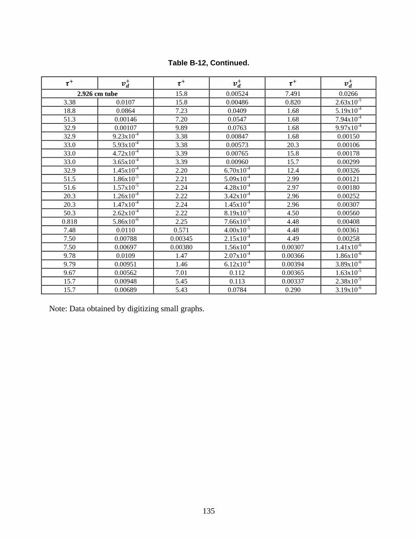
135
Table B-12, Continued.
2.926 cm tube 15.8 0.00524 7.491 0.0266 3.38 0.0107 15.8 0.00486 0.820 2.63x10⁻⁵ 18.8 0.0864 7.23 0.0409 1.68 5.19x10⁻⁴ 51.3 0.00146 7.20 0.0547 1.68 7.94x10⁻⁴ 32.9 0.00107 9.89 0.0763 1.68 9.97x10⁻⁴ 32.9 9.23x10⁻⁴ 3.38 0.00847 1.68 0.00150 33.0 5.93x10⁻⁴ 3.38 0.00573 20.3 0.00106 33.0 4.72x10⁻⁴ 3.39 0.00765 15.8 0.00178 33.0 3.65x10⁻⁴ 3.39 0.00960 15.7 0.00299 32.9 1.45x10⁻⁴ 2.20 6.70x10⁻⁴ 12.4 0.00326 51.5 1.86x10⁻⁵ 2.21 5.09x10⁻⁴ 2.99 0.00121 51.6 1.57x10⁻⁵ 2.24 4.28x10⁻⁴ 2.97 0.00180 20.3 1.26x10⁻⁴ 2.22 3.42x10⁻⁴ 2.96 0.00252 20.3 1.47x10⁻⁴ 2.24 1.45x10⁻⁴ 2.96 0.00307 50.3 2.62x10⁻⁴ 2.22 8.19x10⁻⁵ 4.50 0.00560
0.818 5.86x10⁻⁶ 2.25 7.66x10⁻⁵ 4.48 0.00408 7.48 0.0110 0.571 4.00x10⁻⁵ 4.48 0.00361 7.50 0.00788 0.00345 2.15x10⁻⁴ 4.49 0.00258 7.50 0.00697 0.00380 1.56x10⁻⁴ 0.00307 1.41x10⁻⁶ 9.78 0.0109 1.47 2.07x10⁻⁴ 0.00366 1.86x10⁻⁶ 9.79 0.00951 1.46 6.12x10⁻⁴ 0.00394 3.89x10⁻⁶ 9.67 0.00562 7.01 0.112 0.00365 1.63x10⁻⁵ 15.7 0.00948 5.45 0.113 0.00337 2.38x10⁻⁵ 15.7 0.00689 5.43 0.0784 0.290 3.19x10⁻⁶
Note: Data obtained by digitizing small graphs.
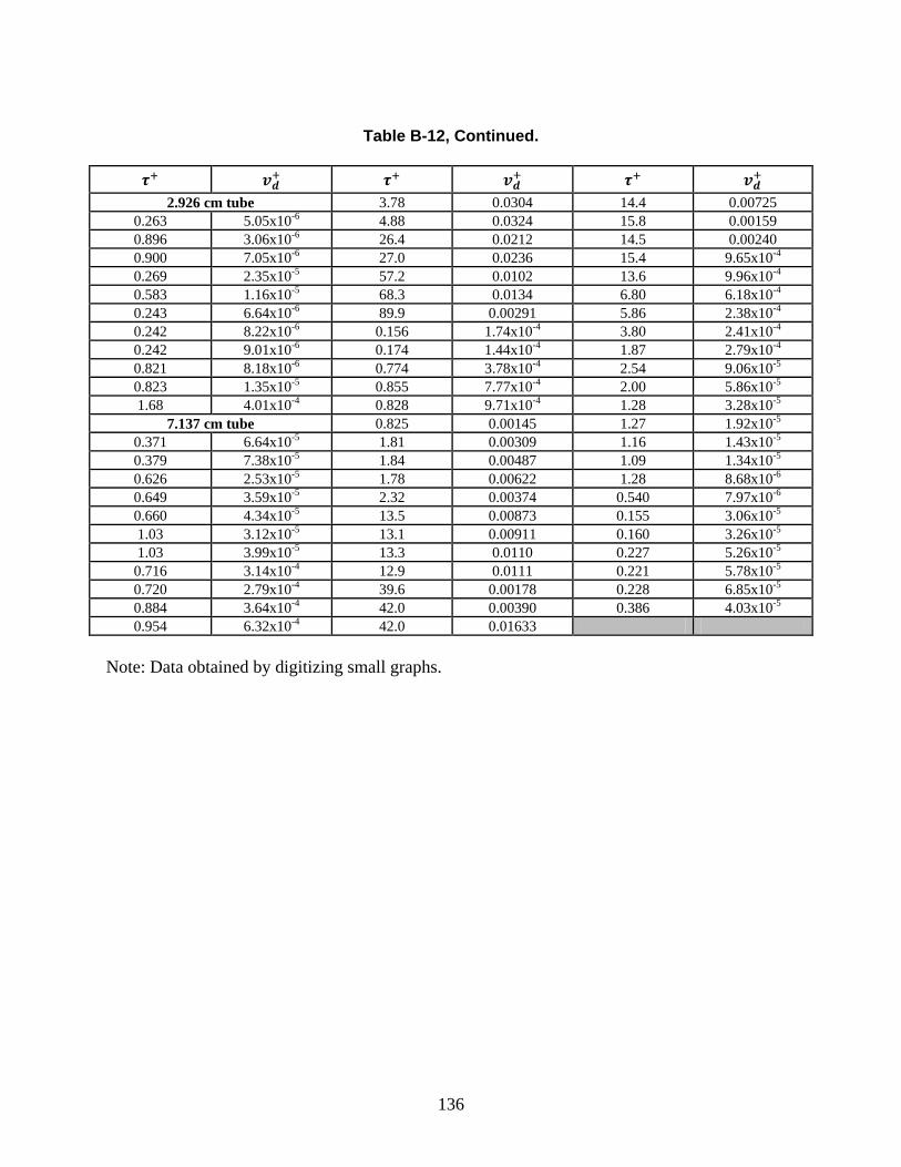
136
Table B-12, Continued.
2.926 cm tube 3.78 0.0304 14.4 0.00725 0.263 5.05x10⁻⁶ 4.88 0.0324 15.8 0.00159 0.896 3.06x10⁻⁶ 26.4 0.0212 14.5 0.00240 0.900 7.05x10⁻⁶ 27.0 0.0236 15.4 9.65x10⁻⁴ 0.269 2.35x10⁻⁵ 57.2 0.0102 13.6 9.96x10⁻⁴ 0.583 1.16x10⁻⁵ 68.3 0.0134 6.80 6.18x10⁻⁴ 0.243 6.64x10⁻⁶ 89.9 0.00291 5.86 2.38x10⁻⁴ 0.242 8.22x10⁻⁶ 0.156 1.74x10⁻⁴ 3.80 2.41x10⁻⁴ 0.242 9.01x10⁻⁶ 0.174 1.44x10⁻⁴ 1.87 2.79x10⁻⁴ 0.821 8.18x10⁻⁶ 0.774 3.78x10⁻⁴ 2.54 9.06x10⁻⁵ 0.823 1.35x10⁻⁵ 0.855 7.77x10⁻⁴ 2.00 5.86x10⁻⁵ 1.68 4.01x10⁻⁴ 0.828 9.71x10⁻⁴ 1.28 3.28x10⁻⁵
7.137 cm tube 0.825 0.00145 1.27 1.92x10⁻⁵ 0.371 6.64x10⁻⁵ 1.81 0.00309 1.16 1.43x10⁻⁵ 0.379 7.38x10⁻⁵ 1.84 0.00487 1.09 1.34x10⁻⁵ 0.626 2.53x10⁻⁵ 1.78 0.00622 1.28 8.68x10⁻⁶ 0.649 3.59x10⁻⁵ 2.32 0.00374 0.540 7.97x10⁻⁶ 0.660 4.34x10⁻⁵ 13.5 0.00873 0.155 3.06x10⁻⁵ 1.03 3.12x10⁻⁵ 13.1 0.00911 0.160 3.26x10⁻⁵ 1.03 3.99x10⁻⁵ 13.3 0.0110 0.227 5.26x10⁻⁵ 0.716 3.14x10⁻⁴ 12.9 0.0111 0.221 5.78x10⁻⁵ 0.720 2.79x10⁻⁴ 39.6 0.00178 0.228 6.85x10⁻⁵ 0.884 3.64x10⁻⁴ 42.0 0.00390 0.386 4.03x10⁻⁵ 0.954 6.32x10⁻⁴ 42.0 0.01633
Note: Data obtained by digitizing small graphs.

138
DISTRIBUTION 2 Jay Lee Mail Stop O10H4 U.S. Nuclear Regulatory Commission
Washington, DC 20555 5 MS0736 Dana A. Powers 6770 1 MS0748 Randall Gauntt 6762 1 MS0748 Donald A. Kalinich 6762 1 MS0899 Technical Library 9536 (electronic copy)