Agricultural Productivity, Technological Change, and Deforestation: A

Global Analysis

Michael Brady* and Brent Sohngen†

This study takes advantages of recent developments in measuring total factor productivity in output specific directions to examine the influence of technological change in different agricultural sectors on land-use decisions in a cross-section of countries from 1969 to 2001. Results demonstrate a positive relationship between productivity and land in agriculture in most cases. The ruminant sector is an exception where an increase in productivity was negatively associated with amount of pastureland. The analysis also includes variables that have been found to be important determinants in other studies of land-use change. Population is clearly the dominant factor over the time period analyzed, although it is argued that other factors are likely to become more important in upcoming years since population growth has slowed significantly in many countries.

Selected Paper prepared for presentation at the American Agricultural Economics

Association Annual Meeting, Orlando, FL, July 27-29, 2008.

_________________________________

* Economic Research Service, U.S. Department of Agriculture, 1800 M Street, NW, Washington DC, 20036. Please do not cite, reproduce, or distribute without permission of the authors. The views expressed are those of the authors and do not necessarily correspond to the views or policies of the Economic Research Service or the U.S. Department of Agriculture. †

Dept. of Agricultural, Environmental, and Development Economics, Ohio State University, 2120 Fyffe Road, Columbus, OH 43212.

1

In this study we examine the relationship between land-use change and agricultural

productivity in a large cross-section of countries over 4 decades to estimate the relationship

between technological change in agriculture and deforestation. The demand for agricultural

production is going to continue to increase as the population approaches 9 billion at mid-

century, per capita incomes continue to rise, and the biofuels sector grows. Whether this can

be achieved without a significant expansion of agricultural land depends largely on the pace

of technological change. This has critical implications for many environmental issues,

particularly with respect to climate change (Searchinger et al., 2007; Feddema et al., 2005;

Tavoni, Sohngen, and Bosetti).

The goal of this paper is not to provide a forecast of global land use change a number

of years forward. That is better done by any number of computable partial and general

equilibrium models. Instead, our contribution is to examine the relationship between rates

of productivity growth across agricultural sectors and land-use change in the recent past to

help understand what may happen in the future. We improve on previous studies by using

output specific measures of total factor productivity (TFP) that disaggregate crops,

ruminants, and non-ruminant livestock. Using output specific measures is important

because technological change occurs independently between sectors, and changes in one

sector can affect another. For instance, an improvement in poultry productivity may

increase the demand for cropland to grow feed grain. Research that has separated sectors

have relied on less accurate partial factor productivity (PFP) measures.

The rapid growth in agricultural productivity beginning in the mid 1960’s was

primarily a result of 4 types of technological advancements; improved germplasm, increased

2

fertilizer use, double cropping, and irrigation (Cassman, 1999). In many industrialized

countries crop yield growth outpaced demand growth resulting in lower prices, a reduction

in agricultural land, and aforestation. At the same time, many developing countries

experienced accelerating deforestation rates largely as a result of agricultural expansion.

This led to concerns about carbon loss and climate change, biodiversity loss, and top soil

loss, to name a few. A number of studies have empirically estimated which factors are the

most important in either decreasing or increasing the expansion of agricultural land. Barbier

and Burgess (1997) and Ehui and Hertel (1989) found that a reduction in forest cover was

associated with increasing population density, while rising income per capita and increasing

agricultural yields led to an increase in forest cover. Another set of papers looking at

household decision-making concluded that increasing agricultural output prices accelerates

the conversion of forest to agriculture, while rural wage rates are positively related to forest

cover (eg. Barbier (2000), Barbier and Burgess (1996), and Lopez (1997)).

We build on these studies by focusing on the relationship between productivity and

land-use between agricultural sectors. The extent to which repercussions of a change in

either the crop or livestock sector are felt in the either have been amplified through the

spread of confined livestock facilities (CAFOs) that use feedgrain to raise animals rather

than pasture grazing. Soybeans, which are a major feed source for pig and poultry

production, were grown minimally relative to rice, wheat, and maize 40 years ago. Today

soybeans cover a significant portion of some of the most productive farmland in the U.S.,

Brazil, and Argentina. Nearly all soybean meal is used to make feed for livestock (ERS).

Livestock productivity in the non-ruminants sector (primarily pigs and poultry) is expected

3

to grow faster than any other agricultural sector in many parts of the world as the use of

CAFOs spread, particularly in China (Ludena et al., 2006).

Meat consumption is also expected to increase significantly for a significant portion

of the world population due to economic growth in countries like China and India. The

average consumption of meat per person in China rose from 20 kg/person/year in 1985 to 50

kg/person/year in 2000 (FAOSTAT). This an important step towards improving living

standards for the world’s poorest people. At the same time, each calorie of meat requires 5

to 10 times as many calories of grain for feed. This raises questions as to whether

productivity growth for crops will be sufficient to prevent a significant expansion of

cropland.

1 Agriculture: The Big Picture

1.1 Production

From the beginning of agriculture in the Neolithic period 12,000 years ago until well

into the 20th century labor was the limiting factor of production in most societies. As a

result, innovation was induced towards creating labor augmenting technologies (Hayami and

Ruttan), which accelerated rapidly after the Industrial Revolution. The ability of each

farmer to tend to greater tracts of land through the use of various tools, culminating with

mechanized tractors, had . First, each farmer produced an increasing amount of excess food

allowing more people to engage in non-farm labor, which in turn led to a rapid increase in

forest clearing for agriculture. As a result, land rather than labor became the scarcer factor

4

reorienting research, particularly in developed countries where most research money is

spent, towards land intensifying technologies throughout the 20th century1.

Figure 1 shows the total production of each of the world’s four crops in 1961 and

2006. All increased significantly, although on a percentage basis the growth in soybeans is

the most dramatic. Figures 2 through 5 track total production, separating out the largest

producers, along with total area. To provide some perspective, about 38% of the total global

land base (13 billion ha) is used for agriculture in some way (FAO, 2007). Arable land

constitutes 11%, 5% contains permanent crops, and 26% is pasture. Figure 6 is an abstract

representation of global land use that provides some perspective of these allocations relative

to other land types.

Soybean production is unique in a number of ways (Figure 2). Maize, rice, and

wheat all show increasing productivity. Total production increased faster than area. While

this was the case for soybeans in the 1990’s the increase in production since has largely been

the result of extensification. Soybean production is also more geographically concentrated

than the other crops. The U.S., Brazil, and Argentina account for nearly all of global

soybean production. Neither South American country produced a significant amount of

soybeans before 1970. Production started to take off in Brazil in the early 1970’s and in

Argentina 10 years later. China is a distant fourth and total production has changed very

little there. This is striking example of the implications that livestock has had on cropland.

Total production of maize continued to increase significantly. Wheat and rice production

1An endogenous factor was the growth in off-farm income which resulted from technological improvements that increase labor productivity.

5

and productivity have slowed. Figures 2 to 5 also show that the amount of land used for rice

and wheat production has flattened while land in maize and soybeans continues to expand.

While yield provides a useful measure of the intensity of production it does not

account for factor substitution. Figure 7 compares trends in world TFP for crops and PFP

for maize, wheat, and rice separately. TFP for crops is lower than each PFP measure

because it accounts for increased use of non-land inputs. Figure 7 also shows why it is

important to delineate between agricultural sectors even within livestock. Growth in non-

ruminant TFP was larger than that for ruminants. There is significant variation across

regions as well. Industrialized countries made their biggest gains in crops and ruminants

while China dominated growth in non-ruminant productivity. Regions like Sub-Saharan

Africa and the Middle East made little improvement in productivity in any sector, which was

likely both a cause and effect of stagnating living standards in those areas.

1.2 Consumption

For the next few decades increasing demand will come from growth in population

and income. Higher income increases overall food consumption, but also increases the

prevalence of meat in diets. Approximately 16% of income in rich countries is spent on

food compared to 55% in poor countries (ERS, 1997). In 2002, the highest consumption in

countries including the United States was approximately 124 kg/person/year, which was up

85% from 1970. Bangladesh consumes the least meat at 3.1 kg/person/year. About 30% of

total dietary energy consumption for people in the U.S. is from animal products compared to

3% for Bangladesh. Projections assert that 85% of the growth in food demand to 2020 will

come from developing countries where the demand for meat could double over this time

period (Andersen, Pandya-Lorch, and Rosegrant, 1999 via ERS WRS-011-1).

6

A scatterplot of meat consumption (kg/person/year) and GDP per capita (current US

dollars) for most countries in the world in 2002 (Figure 6.1) shows the positive correlation

between income and meat consumption (FAOSTAT). The size of the bubbles reflects the

population of the country. A simple regression analysis shows that a 1% increase in GDP

per capita leads to a 0.48% increase in meat consumption. The relationship is concave2 so

meat consumption can be expected to increase as incomes grow from low levels but from

medium to high income the relationship decelerates. Both graphs in Figure 6.1 show that

increased demand for meat could have huge land use implications in the near future because

the majority of the global population resides in the region where meat consumption

increases significantly with income growth.

1.3 Trade

Currently, 10% of global agricultural production is traded internationally in terms of

quantity (Tubiello, Soussana, and Howden, 2007). The effect of increased demand from

China for animal feed on cropland demand in South America is likely to be the most

important factor affecting global land use change in the near future. Countries have also

started trading more processed meats, although countries with increasing meat consumption

have not increased meat imports. Domestic production has met increased demand in most

cases. Trade in feed grains has shifted from developed to developing countries, particularly

soybean meal, explaining why soybeans have passed wheat as the most traded cereal grain.

Coyle, et al. (1998) found income change to be the most important variable in explaining

changes in trade patterns.

2 Based on the coefficient estimates for GDP per capita and it’s square.

7

2 Variable Description

This analysis is modest in terms of the structure it imposes on the dynamics of land

use change. Using a large sample of countries over 30 years provides an amount of

variation needed to assess land use change that can be relatively slow. At the same time, it

presents difficulties in formulating an applicable set of assumptions on the nature of land use

change across the sample. Angelsen’s (1999) summary of land use models shows how the

dynamics of land use change depend on assumptions about household objective functions,

trade policy, farm and off-farm labor markets3, and property rights4. Our approach then is

to investigate within a simple framework i) what relationships predominate between sub-

sector productivity change and agricultural land use change, and ii) how strong the

relationship between productivity and land use change is relative to other factors. These

include population, population density, income, property rights institutions, and agricultural

productivity.

Using output specific TFP measures for 127 countries from Ludena et al. (2007), a

set of panel data specifications are used covering the years from 1968 to 2000. The

dependent variables are two categories of agricultural land-use from the FAO; arable land

and permanent crops (ALPC), and pasture and rangeland (PAST). The explanatory

3Household preferences focus primarily on the labor/leisure tradeoff. ‘Traditional’ societies display lexicographic preferences where they are not willing to trade leisure for labor once subsistence consumption requirements are met. This is largely a result of not being integrated into a larger economy. Models also vary the level of market integration primarily with respect to labor, which is critical in determining the relationship between productivity and land-use. Labor markets are assumed to take one of three forms. First, no off-farm employment options exist. Second, imperfect labor markets are present, but the household is quantity constrained. Third, labor markets are perfect for both buying and selling labor time.

4 Assumptions about property rights regimes are categorized as being a system of complete private or communal rights for both forest and cultivated land, pure open access, or partial open access. The last category applies to countries with land tenure laws where forests have no de facto ownership, but clearing and using land for agricultural production can lead to ownership. This is also referred to as homesteading, or ax rights.

8

variables include lagged values for population, population density, property rights

institutions, and TFP measures for crops and livestock.

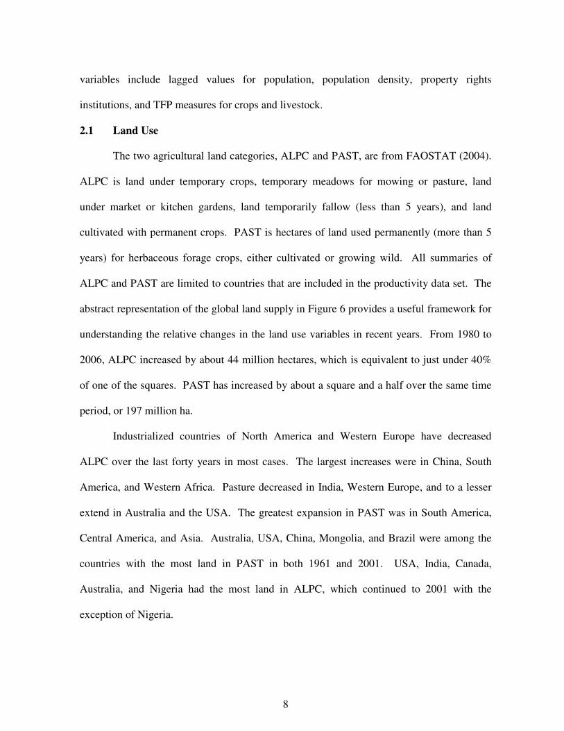
2.1 Land Use

The two agricultural land categories, ALPC and PAST, are from FAOSTAT (2004).

ALPC is land under temporary crops, temporary meadows for mowing or pasture, land

under market or kitchen gardens, land temporarily fallow (less than 5 years), and land

cultivated with permanent crops. PAST is hectares of land used permanently (more than 5

years) for herbaceous forage crops, either cultivated or growing wild. All summaries of

ALPC and PAST are limited to countries that are included in the productivity data set. The

abstract representation of the global land supply in Figure 6 provides a useful framework for

understanding the relative changes in the land use variables in recent years. From 1980 to

2006, ALPC increased by about 44 million hectares, which is equivalent to just under 40%

of one of the squares. PAST has increased by about a square and a half over the same time

period, or 197 million ha.

Industrialized countries of North America and Western Europe have decreased

ALPC over the last forty years in most cases. The largest increases were in China, South

America, and Western Africa. Pasture decreased in India, Western Europe, and to a lesser

extend in Australia and the USA. The greatest expansion in PAST was in South America,

Central America, and Asia. Australia, USA, China, Mongolia, and Brazil were among the

countries with the most land in PAST in both 1961 and 2001. USA, India, Canada,

Australia, and Nigeria had the most land in ALPC, which continued to 2001 with the

exception of Nigeria.

9

2.2 Productivity

The total factor productivity (TFP) measure is based on a directional distance

function (DDF) approach (Chambers, et al. 1996). Details on how TFP is measured using a

DDF approach can be found in Nin et al. (2003) and Ludena et al. (2007). Input and output

variables are from FAOSTAT (2004), the database from the Food and Agriculture

Organization of the United Nations. Inputs are feed, animal stock, pasture, land under crops,

fertilizer, tractors, and labor. Outputs are crops, ruminants, and non-ruminants livestock.

A significant drawback with directional measures is that there is sometimes no

solution to the linear programming problem when measuring productivity in an output

specific direction. This tends to occur when a production unit is near the efficient frontier.

We attempt to “smooth” over the some of the missing observations by transforming the

productivity number into a lagged mean. This also smooths over year to year fluctuations in

productivity from weather. We only include a country in the sample if it has at least half of

the observations for the years from 1961 to 2001.

The average annual percentage change for crops and livestock by country from 1961

to 2001 is shown in Figures 8 and 9. Extreme values are partially a result of some countries

having very few observations due to the solution problem described above. These are not

included in the sample for statistical analysis. World agriculture TFP has grown at just

under 1% per year over this time. As expected, countries in North America and Western

Europe increased productivity in agriculture significantly relative to the rest of the world.

That said, there were a number of less developed countries in South America, parts of

Africa, and Southeast Asia that experienced significant gains in productivity. Many

countries that have been associated with rapid deforestation and loss of natural habitat

10

achieved more modest productivity increases, such as Brazil, countries in Western Africa,

and India.

Growth in non-ruminants productivity has been the largest among the agricultural

sectors. Average annual percentage growth rates are estimated at 2.6% compared to 0.62%

for ruminants. The performance in the non-ruminant sector has largely resulted from

improved feed and controlled industrial facilities. There is trend across developed

industrialized countries for greater productivity gains in crops than for livestock. For

example, Western Europe collectively achieved an annual percentage growth rate for crops

of 2.5% compared to 1.19% for livestock.

2.3 Other Determinants of Land-Use

Other variables that have been shown to influence land-use change are GDP per

capita as a measure of income, population, population density, and political institutions.

Data for GDP per capita is from The World Bank national accounts data and is measured in

constant 2000 $US. The wealthiest countries in 1965 not only remained the wealthiest in

2001 but also became relatively more wealthy. GDP per capita increased on average at

2.4% per year for the wealthiest countries. Living standards in the former Soviet block

countries and the Middle East and North Africa were stagnant. The largest rate of

improvement was in Asia where many of the ‘Asian Tigers’ achieved rapid economic

growth. Income improved slightly in Latin America. The poorest countries in both 1965

and 2001 were primarily in Sub-Saharan Africa.

We include both population and population density. Countries with a large land

mass may be able to accommodate a rapidly growing population without people being

11

driven out in the countryside if levels remain below a threshold, such as is the case in the

U.S. and Canada.

A number of studies have empirically estimated a statistically significant relationship

between land-use change and the political and institutional makeup of countries. The

general hypothesis is that poor institutions lead to a weak system of property rights which is

necessary to avoid problems associated with the overuse of open access resources. The

primary difficulty in this line of analysis is creating a representative variable or set of

variables that adequately capture the strength of political and economic institutions. We use

indexes for property rights is produced by Freedom House and is used here. It ranks

countries on a 5 point scale where 1 is strong property rights and 5 is weak. The drawback

is that it is not until the year 2000 that observations are available for nearly all the countries

in the productivity sample. Therefore, analysis including the property rights variable will be

limited to years after 1990. Going further back would make it more likely that significant

institutional change has taken place. Using only a single observation for each country

requires using a random effects model instead of fixed effects, which does improve

efficiency of estimation but introduces greater risk for bias.

3 Regression Analysis

While lagged observations are used for all independent variables productivity differs

slightly. As mentioned earlier, the average of the previous four years of annual productivity

change observations is used to reduce loss of observations from missing data, and to smooth

out weather shocks. Since the variable is a percentage change the geometric mean is used.

The other variables are simply a one period lag.

12

This design has two motivations. First, planting decisions in agriculture are discrete

in that they are made at the beginning of the year and can rarely be changed until the

following year. For productivity four years is used because it is long enough to smooth out

year to year fluctuations, but is also short enough to capture changes in values of variables

over time. Results did not change significantly using 3 or 5 year lags. This general length

of time has also been used in other studies. Deacon (1994) used 5 year non-overlapping

blocks.

The primary regression framework used is a fixed effects panel model. This has the

advantage of avoiding bias resulting from correlation between unobserved country

characteristics that do not change over time, such as whether it is landlocked, and the

included regressors. The model follows the general fixed effects transformation of

differencing by the group mean

Ttuuxxyy iitiitiit ,....,2,1,)(__

1

_

=−+−=− β

which is estimated using OLS with a constant 0β . This assumes the demeaned errors are

homoskedastic and serially uncorrelated. To partially guard against bias resulting from the

violation of these assumptions robust standard errors are used throughout.

3.1 Aggregate Agriculture

Table 1 shows results for the the dependent variable that is the sum of PAST and

ALPC. Explanatory variables include TFP for agriculture, not output specific, GDP per

capita, population, and population density as the set of explanatory variables from 1969 to

2001. While some of the data is available back to 1961 the panel does not start until 1969

because it reduces missing observations for GDP per capita in the mid 1960’s, and the four

13

period lagged mean for productivity means that the first land-use observation that can be

used is 1966. Using agricultural land variables and TFP for agriculture is a less precise

analysis than what follows, but it provides a useful general overview of the relationships

among the variables. It also avoids the missing data problem for productivity since it is not

an output specific measure.

The p-value for all coefficients is less than 0.05. The relationship between

productivity and land is positive. The coefficient estimate implies that an average increase

in productivity of 1% over the previous four years is associated with an increase of 62,000

ha of land in agriculture. Put into perspective, Japan has approximately 5,000,000 ha of

arable and pastureland combined, which constitutes about 1/7th of the total land mass. An

increase in GDP per capita was inversely related to agricultural land. A significant number

of countries did not have observations for GDP per capita in 1965, although the number

decreases quickly moving into the 1970’s and 80’s. For obvious reasons related to reporting

and monitoring poorer countries were more likely to be missing observations early on. The

average value for 2001 GDP per capita for a country with an observation for 1965 was

$7000, while it was $2500 for those without. So, a $1000 increase in GDP per capita leads

to a decrease in agricultural land of 100,000 ha. Some countries achieved an increase much

greater than $1000 over the time period while others do not come close. Bangladesh only

increased GDP per capita from $103 to $353 over the 30 year period. Australia on the other

hand managed to grow from about $2000 to $20,000.

The sign of the coefficient is negative for population density and positive for raw

population, but this is likely due to collinearity between the two variables. Population

appears to be the more significant measure. Running the same regression without

14

population density changes the coefficient on population very little. If population is dropped

the coefficient on density is positive and significant. Population is measured in millions, so

an increase in population of 1 million people corresponds with an increase in agricultural

land of 178,000 ha. For an average country in the sample this is about a 3% increase. Even

though the coefficients for all the explanatory variables were significant a comparison of the

values for overall R-square demonstrates that population has the most power in explaining

variation in the dependent variable. The right column in Table 1 shows the R-square for the

model when dropping the variable on that line. The value changes very little when

productivity and GDP per capita are not included. When population is dropped the value

decreases by a factor of 10 from about 0.3 to 0.02.

3.2 Sector Specific Regressions

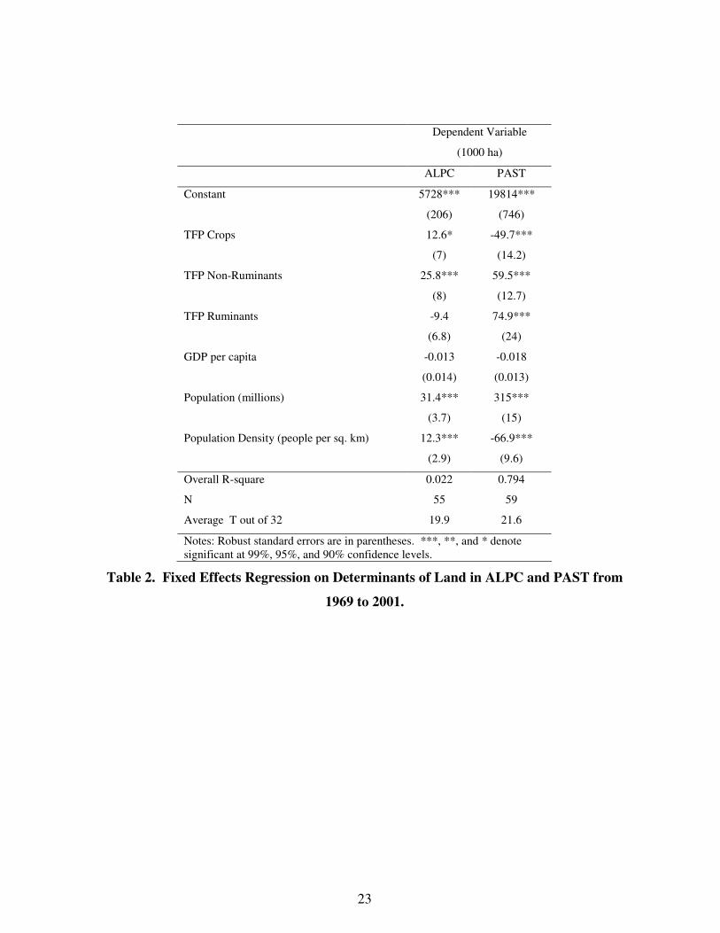
Table 2 displays results from a model that takes advantage of the ability to measure

productivity change with respect to specific sub-sectors of outputs within agriculture. This

also motivates separating land into ALPC and PAST to isolate the effect of each explanatory

variable on land allocated towards growing crops versus livestock. The productivity

measures for crops, ruminants, and non-ruminants are all included for regressions for both

ALPC and PAST because productivity change in each sector can have an influence on each

type of land-use. The sample consists of only countries that had more than half of the

productivity observations for all three of the sub-sectors.

The relationship between crop productivity and ALPC and PAST displays what has

been generally found in developed industrialized countries over the last few decades where

there has been a net loss in agricultural land. This may be partially a result of increasing

crop productivity, which was much higher in wealthier countries where some pastureland

15

was converted to grow crops or was taken out of production. This also comes through in the

fact that the coefficient on crop productivity in the PAST regression is about 4 times as large

as that for the ALPC regression. To reiterate, all coefficients on productivity variables

range between 10 and 50 meaning a 1% increase in productivity leads to an expansion or

contraction, depending on the sign, of 10,000 ha to 50,000 ha.

This relationship between crop productivity and the change in allocation of land has

interesting environmental implications. Countries like the U.S. have managed to increase

forested land because the decrease in pasture has been larger than the increase in cropland.

Therefore, there is a positive effect on decreasing deforestation. At the same time, crop

production generally carries with it an increase in the use of chemical additives, which have

significant environmental impacts, particularly on water related resources.

Increasing productivity in the non-ruminant sector was associated with an increase in

both ALPC and PAST significant at a confidence level greater than 99% in both cases. A

significant cause of productivity gains in developed countries in the pig and poultry sectors

has been related to the science of feed (Nin et al. 2003). It is possible that this increased

demand for crops that produce grains for animal feed. In the case of China Ludena et al.

attribute the rapid increase in non-ruminant productivity to a process of ‘catching-up’ to

methods already existing in developed countries that were adopted quickly once some

element of private ownership was introduced into the agriculture sector around 1980. This

mainly had to do with increased use of confined production systems.

Productivity gains in the ruminant sector have been more modest in general. Only

China stands out as having achieved particularly strong improvements. Ruminant

productivity is not significantly related to ALPC, but does show a positive and significant

16

relationship with PAST. This makes intuitive sense given that non-ruminant livestock rely

primarily on pasture grazing. Although, corn has become an important feed stock for cattle

in the U.S. and some other countries. It is interesting to view these results in the context of

which shows that countries with the largest increases in PAST include Brazil and China.

Latin America has achieved greater increases in ruminant productivity from 1980 to 2000

than industrialized countries after having made no gains at all in the previous 20 years. It is

over this time period of realizing productivity gains that the rate of reduction of the

rainforest has quickened. These results provide some evidence that increased productivity in

ruminants has not slowed the rate of clearing.

Turning to the non-productivity related explanatory variables reveals that GDP per

capita is not significantly related to either land variable in isolation. Population remains

highly significant and positive for both ALPC and PAST. For ALPC, population density is

significant even when population is included. As was true for the agriculture regression in

Table 1, population density becomes positive and significant when population is dropped.

Another interesting difference between the ALPC and PAST regressions is the difference in

the overall R-square. Compared to other regressions in this study the R-square for PAST is

very high considering the included regressors explain about 70% of the overall variation in

permanent pasture and meadows. Alternatively, R-square for ALPC is more than a factor of

10 smaller at 0.02. This could mean that population change has very significant effects on

pasture, but much less so on cropland. In terms of ALPC there is likely additional factors

that influence cropland decisions which should be investigated in future research. A likely

candidate is output prices for agricultural goods. As mentioned earlier, it is additionally

17

important given the confluence of predictions provided by increasing productivity and

prices.

3.3 Property Rights

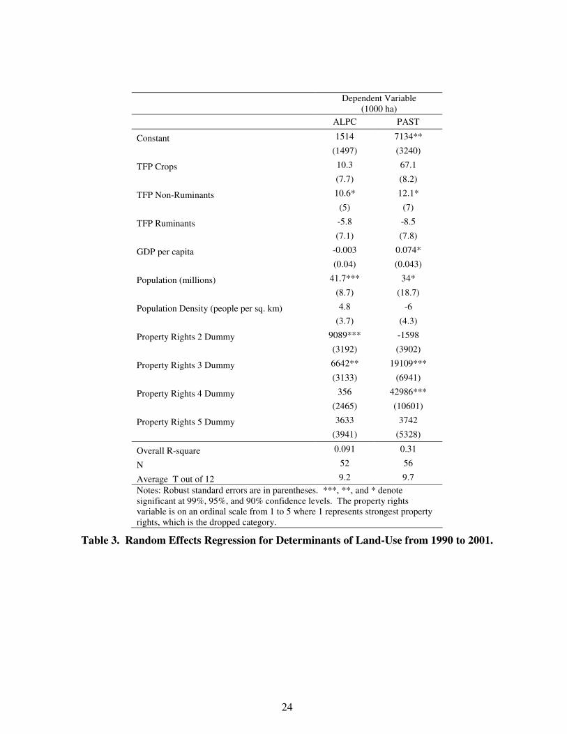
Table 3 shows results from a random effects regression that includes dummy

variables for strength of property rights institutions from Freedom House. A random effects

model is necessary because only one observation is available for each country, which

applies to the year 2000. The sample is limited to the period from 1990 to 2001 to increase

the relevance of the 2000 observation to each year in the sample. Again, the property rights

variable is reported on a scale of 1 to 5 increasing inversely with strength of property rights.

To discern between different levels of strength the ordinal variable is converted to a set of

dummies. Category 1 is dropped. Most Western European and North American countries

have a score of 1. Brazil has a score of 3, while countries such as the Congo and Haiti are

rated at 5.

Results show that weaker property rights are associated with increasing land in

agriculture to a point. The trend does not hold over the entire range of the variable.

Compared to countries with full and complete property rights institutions those with scores

of 2 and 3 have greater land in ALPC, but this is not so for countries with scores of 4 and 5.

For PAST there is no difference between 1 and 2, but countries with scores of 3 and 4 have

more land in PAST. While there could be signs of an interesting difference between PAST

and ALPC being demonstrated here the lack of precision of the property rights variable

given the time displacement issue make it unwise to draw overly strong conclusions.

This regression also provides an interesting comparison for different time periods by

focusing on the later years in the sample. Estimates are insignificant for both crops and

18

ruminants, but remain moderately significant and positive for non-ruminants in terms of

both dependent variables. The most difference is for population. Comparing coefficients

for the two dependent variables show that they are similar in magnitude, which is surprising

since that for PAST tended to be larger when considering the full time period. The

coefficient is also significant at a much higher confidence level for ALPC compared to

PAST.

4 Conclusions

This study analyzed the determinants of land-use change in agriculture building on

previous studies by incorporating total factor productivity measures that isolate

technological change in different agricultural sectors. This is important for a number of

reasons. The production of crops and different types of livestock experience technological

change at varying times and rates. This is a fact that would not be captured with a general

measure of agricultural productivity. Different sectors of agriculture also have unique

environmental repercussions. Lastly, mechanisms exist that allow productivity change in

one sector to influence land-use change in another. For example, the demand for grain for

livestock feed has dramatic implications in terms of allocating land to crop production.

Results showed that increased productivity in different sectors of agriculture was

most often associated with agricultural expansion, although this is by no means the entire

story. Countries with increased crop productivity decreased land in pasture. This

relationship was common in industrialized nations. Increased productivity in the non-

ruminants sector was associated with increases in both ALPC and PAST. It is

understandable how the association would exist for ALPC from increased demand for feed

19

grain. It is less obvious how non-ruminants could be connected to changes in PAST since

they are not grazed. Weaker property rights were associated with an more land in

agriculture, although this result primarily existed for countries in the middle of the scale

relative to countries with the strongest institutions defining ownership. While all the

included variables demonstrated some relationship with land-use change population was

clearly the most important in terms of explaining the variation in land-use.

20

5 References Barbier, E. 2001. The Economics of Tropical Deforestation and Land Use: An Introduction to the Special Issue. Land Economics 77(2):155-171. Barbier, E. and J. Burgess. 1996. Economic Analysis of Deforestation in Mexico. Environment and Development Economics 1(2):203-240. Becker G., E. Glaeser, and K. Murphy. 1999. Population and Economic Growth. American

Economic Review 89(2):145-149. Bohn H. and R. Deacon. 2000. Ownership Risk, Investment, and the Use of Natural Resources. The American Economic Review 90(3):526-549. Brandao, A., and J. Carvalho. “Brazil”. The Political Economy of Agricultural Pricing

Policy. A. Krueger, M. Schiff and A. Valdes. eds. pp. 52-99. Baltimore: Johns Hopkins University Press. 1992. Chambers, R., Y. Chung, and R. Fare. Benefit and distance functions. Journal of Economic

Theory 70(2):407-419. Ehui, S., and T. Hertel. 1989. Deforestation and Agricultural Productivity in the Cote d’Ivoire. American Journal of Agricultural Economics 71:703-711. FAO (Food and Agriculture Organization of the United Nations). FAOSTAT database. http://faostat.fao.org. Food and Agriculture Organization. United Nations. The State of Food and Agriculture, 2007. FRA. United Nations Food and Agriculture Organization (FAO). Global Forest Resources

Assessment. Rome: United Nations, 2005. Freedom House. Freedom in the World: The Annual Survey of Political Rights & Civil

Liberties: 2001-2002. New Brunswick, NJ: Freedom House, 2006. Hayami, Y., and V. Ruttan. 1970. Agricultural productivity differences among countries. American Economic Review 60:895-911. Koop, G., and L. Toole. 1999. Is There an Environmental Kuznets Curve for Deforestation? Journal of Development Economics 58:231-244. Kormendi, R, and P. Meguire. 1985. Macroeconomic Determinants of Growth: Cross-Country Evidence. Journal of Monetary Economics 16(2):141-63.

21

Lopez, R. 1997. Environmental Externalities in Traditional Agriculture and the Impact of Trade Liberalization: The Case of Ghana. Journal of Development Economics 53:17-39. Nin, A., C. Arndt, T. Hertel, and P. Preckel. 2003. Bridging the gap between partial and total factor productivity measures using directional distance functions. American Journal of

Agricultural Economics 85(4):928-942. Nadiri, M. 1970. Some approaches to the theory and measurement of total factor productivity: A survey. Journal of Economic Literature 8(4):1137-1177. Panayatou, T., and S. Sungsuwan. 1994. An Econometric Analysis of the Causes of Tropical Deforestation: The Case of Northeast Thailand. In The Causes of Tropical Deforestation:

The Economic and Statistical Analysis of Factors Giving Rise to the Loss of Tropical

Forests. ed. K. Brown and D.W. Pearce, 192-210. London: University College Press. Restuccia, D. 2004. Barriers to Capital Accumulation and Aggregate Total Factor Productivity. International Economic Review 45(1):225-38. Shafik, N. 1994. Economic Development and Environmental Quality: An Econometric Analysis. Oxford Economic Papers 46:757-773.

22

Tables

Dependent Variable = ALPC + PAST (1000 ha)

Estimate

Overall R-square

without

Constant 33189***

(828)

TFP Agriculture 62** 0.341

(20)

GDP per capita -0.1*** 0.343

(0.023)

Population (millions) 178*** 0.021

(26)

Population Density

(people per sq. km) -34*** 0.306

(4.9)

Overall R-square 0.342

N 102

Average T out of 32 29.6

Notes: Robust standard errors are in parentheses. ***, **, and * denote significant at 99%, 95%, and 90% confidence levels. The R-square without column provides the percent of overall variation in the dependent variable explained by all the listed regressors except the one on that row.

Table 1. Fixed Effects Regression on Determinants of Land Under Crops and Pasture

from 1969 to 2001.

23

Dependent Variable

(1000 ha)

ALPC PAST

Constant 5728*** 19814***

(206) (746)

TFP Crops 12.6* -49.7***

(7) (14.2)

TFP Non-Ruminants 25.8*** 59.5***

(8) (12.7)

TFP Ruminants -9.4 74.9***

(6.8) (24)

GDP per capita -0.013 -0.018

(0.014) (0.013)

Population (millions) 31.4*** 315***

(3.7) (15)

Population Density (people per sq. km) 12.3*** -66.9***

(2.9) (9.6)

Overall R-square 0.022 0.794

N 55 59

Average T out of 32 19.9 21.6

Notes: Robust standard errors are in parentheses. ***, **, and * denote significant at 99%, 95%, and 90% confidence levels.

Table 2. Fixed Effects Regression on Determinants of Land in ALPC and PAST from

1969 to 2001.

24

Dependent Variable

(1000 ha)

ALPC PAST

Constant 1514 7134**

(1497) (3240)

TFP Crops 10.3 67.1

(7.7) (8.2)

TFP Non-Ruminants 10.6* 12.1*

(5) (7)

TFP Ruminants -5.8 -8.5

(7.1) (7.8)

GDP per capita -0.003 0.074*

(0.04) (0.043)

Population (millions) 41.7*** 34*

(8.7) (18.7)

Population Density (people per sq. km) 4.8 -6

(3.7) (4.3)

Property Rights 2 Dummy 9089*** -1598

(3192) (3902)

Property Rights 3 Dummy 6642** 19109***

(3133) (6941)

Property Rights 4 Dummy 356 42986***

(2465) (10601)

Property Rights 5 Dummy 3633 3742

(3941) (5328)

Overall R-square 0.091 0.31

N 52 56

Average T out of 12 9.2 9.7

Notes: Robust standard errors are in parentheses. ***, **, and * denote significant at 99%, 95%, and 90% confidence levels. The property rights variable is on an ordinal scale from 1 to 5 where 1 represents strongest property rights, which is the dropped category.

Table 3. Random Effects Regression for Determinants of Land-Use from 1990 to 2001.

25

Million Tons Produced

0

500

1000

1500

2000

2500

1961 2006

Wheat

Maize

Rice

Soybeans

Figure 5. Total Global Production of the 4 Major Crops.

26

Soybeans

0

50

100

150

200

250

1961

1963

1965

1967

1969

1971

1973

1975

1977

1979

1981

1983

1985

1987

1989

1991

1993

1995

1997

1999

2001

2003

2005

Mill

ion

To

ns

0

20

40

60

80

100

Mill

ion H

ecta

res Rest of World

China

Argentina

Brazil

USA

Area

Figure 2. Soybean Production and Area.

Rice

0

100

200

300

400

500

600

700

1961

1963

1965

1967

1969

1971

1973

1975

1977

1979

1981

1983

1985

1987

1989

1991

1993

1995

1997

1999

2001

2003

2005

Mill

ion

To

ns

0

20

40

60

80

100

120

140

160

180

Mill

ion

He

cta

res

Rest of World

Thailand

Viet Nam

Bangladesh

Indonesia

India

China

Area

Figure 3. Rice Production and Area.

27

Maize

0

100

200

300

400

500

600

700

800

1961

1963

1965

1967

1969

1971

1973

1975

1977

1979

1981

1983

1985

1987

1989

1991

1993

1995

1997

1999

2001

2003

2005

Mill

ion T

on

s

0

20

40

60

80

100

120

140

160

Mill

ion H

ecta

res

Rest of World

Argentina

India

Mexico

Brazil

China

USA

Area

Figure 4. Maize Production and Area.

Wheat

0

100

200

300

400

500

600

700

800

900

1961

1963

1965

1967

1969

1971

1973

1975

1977

1979

1981

1983

1985

1987

1989

1991

1993

1995

1997

1999

2001

2003

2005

Mill

ion T

ons

0

50

100

150

200

250

300

Mill

ion H

ecta

res

Rest of World

Germany

Canada

France

USA

India

USSR (former)

China

Area

Figure 5. Wheat Production and Area.

28

Figure 6. An Abstract Representation of the Allocation of the Global Land Base.

Global Land Base Allocation in 2006

(13 Billion Hectares)

Tropical Forest

Grassland and Pasture

Other

Subtropical Forest

Temperate Forest

Boreal Forest

Arable Land

Permanent Crops

Note: One square is equal to approximately 130 million hectares.

Cropland added from 1980 to 2006

29

Bubble Size Reflects Country Population

-40

-20

0

20

40

60

80

100

120

140

160

180

-5000 5000 15000 25000 35000 45000 55000 65000

GDP Per capita

Me

at C

on

su

mp

tion

by C

ou

ntr

y

(kg

/pe

rso

n/y

ea

r)

Figure 6.1. GDP per capita and Meat Consumption per capita in 2002.

30

0

0.5

1

1.5

2

2.5

3

1961

1963

1965

1967

1969

1971

1973

1975

1977

1979

1981

1983

1985

1987

1989

1991

1993

1995

1997

1999

Cum

ula

tive P

erc

enta

ge C

hange

Crops TFP Rum TFP NR TFP Maize PFP Rice PFP Wheat PFP

Figure 7. World Crop TFP and Commodity Specific PFP Cumulative Percentage

Change.

31

Figure 8. Average Annual Change in Crop Total Factor Productivity from 1961 to

2001.

32

Figure 9. Average Annual Change in Livestock Total Factor Productivity from

1961 to 2001.