air speed measurement standards using wind tunnels

9

Air Speed Measurement Standards Using Wind Tunnels

Sejong Chun Korea Research Institute of Standards and Science

Korea

1. Introduction

Accurate air speed measurement is essential to understand flow phenomena and practical engineering problems, such as wind turbines, air ventilation systems, air filter testers, and fan testers, etc. Standard wind tunnels can provide good testing environments for calibrating and testing industrial anemometers, which are widely used for measuring air speeds in applications to various on-site air speed measurements. Air speed standards can be established by adopting a wind tunnel. In this case, some knowledges are required, regarding measurement accuracy and uncertainty assessment. To certify an industrial anemometer, a calibration certificate is issued by an accredited laboratory, which is recognized by an accreditation organization in a country, according to the ISO/IEC 17025 guide (ISO, 2005). The national metrology institutes in every country advise the accreditation organization in recognizing the accredited laboratory by providing technical supports with the national measurement standards. Traceability is established from the national standards to the industrial standards, by transferring national measurement standards from the national metrology institutes to the accredited laboratories. If an industrial anemometer is exported to a foreign country, an international calibration certification must be issued to provide the measurement accuracy requested by a customer in the foreign country. Mutual recognition arrangement realizes the international certification procedures by harmonizing the calibration and measurement capability (CMC) of industrial countries. International key comparisons are performed to fulfill the purpose of the mutual recognition arrangement. The international key comparisons are managed by the CIPM. In case of air speed metrology, three international key comparisons have been conducted by either world-wide or regional levels, up to date. In this book chapter, a brief explanation, regarding the air speed metrology, is introduced. At first, some basics of statistical methods to calibrate an industrial anemometer are explained. After that, an air speed metrology is briefly introduced by considering the traceability chain from the national measurement standards to the industrial or working standards, based on the literature. Finally, some information, regarding the mutual recognition arrangement and the international key comparisons, will be mentioned. From this approach, it is expected that some basic knowledge of the air speed metrology can be useful in understanding how to measure the industrial anemometers with good measurement accuracy and uncertainty.

www.intechopen.com

Wind Tunnels and Experimental Fluid Dynamics Research 174

2. Basics of statistics for calibration of an anemometer

2.1 Basics of uncertainty measurement When an anemometer is calibrated, people consider statistics because the measurement data for anemometer calibration generates statistical distributions. To determine a calibration coefficient of the anemometer, statistical moments such as a mean and a standard deviation are considered (Dougherty, 1990). Because the mean is an unbiased estimator, it is believed that the mean value approaches to the true value by measuring the data with infinite times. In this case, the standard uncertainty to determine the mean value becomes zero, according to the following equation.

購掴̅ = 蹄猫√津 (1)

Here, 捲̅ is the mean value of 岶捲沈 , 件 = な,に, … , 券岼, 券 is the number of measurement, 購掴 is the standard deviation of 捲沈, and 購掴̅ is the standard deviation of 捲̅. 購掴̅ is referred to as the standard uncertainty, or more exactly, type A uncertainty (BIPM et al., 1993). The type A uncertainty is related with direct measurement when the device under test, or the 経戟劇 is calibrated. On the contrary, the uncertainty component, which is not directly related to the measurement, is referred to be type B uncertainty. The type B uncertainty includes all the other information except measurement, such as the standard uncertainty of an apparatus written in a calibration certificate, or a nominal value defined in a table, etc. When determining the type A uncertainty, they can assume that the measuring quantity has the Gaussian distribution as a probability density function, by applying the central limit theorem (Dougherty, 1990). To assume the Gaussian distribution, the number of samples should be at least more than 50. However, in some cases, it is possible to assume the Gaussian distribution with the number of data more than 30. In case that the number of data is less than 10, the Student-建 distribution is assumed. The difference between the Gaussian and the Student-建 distribution is the value of coverage factor, 倦 with the same confidence intervals of, e.g., 95 %. 倦 is a necessary quantity when an expanded uncertainty is estimated based on a combined uncertainty, which combines the type A and the type B uncertainties (BIPM et al., 1993). When determining the type B uncertainty, a rectangular, a triangular, and a trapezoidal distribution are usually assumed according to data types. In most cases, the rectangular distribution is preferred to represent the type B uncertainty, when a value is referred from tables, or calibration certificates, etc. Some of values of 倦 for different probability distributions are summarized in Table 1.

Distribution Coverage factor 倦U-shaped √に

Retangular √ぬTriangular √はGaussian 1.96

Student – t

12.71 荒 = 14.30 荒 = 22.57 荒 =5

2.23 荒 = 102.09 荒 = 202.04 荒 = 30

Table 1. Coverage factor 倦 with confidence level of 95 %

www.intechopen.com

Air Speed Measurement Standards Using Wind Tunnels 175

Measurement uncertainty is a combination of estimated uncertainties of each component,

recognized as an uncertainty factor to a measuring quantity. The combined uncertainty is

calculated according to the following formula (Kirkup & Frenkel, 2006).

憲 = 紐憲凋態 + 憲喋態 (2)

Here, 憲凋 denotes the type A uncertainty, 憲喋 denotes the type B uncertainty, and 憲 is the combined uncertainty. The Equation (2) combines 憲凋 and 憲喋 by a vector sum, because the two types of uncertainties are assumed to be independent and uncorrelated with each other. However, there are some cases where the uncertainty factors are not independent and uncorrelated. In these cases, correlation coefficients among the uncertainty factors must be calculated (Kirkup & Frenkel, 2006). To calculate the expanded uncertainty, the coverage factor 倦 is multiplied to the combined uncertainty, as follows.

戟 = 倦憲 (3)

Because the confidence interval with 95 % is widely accepted, 倦 can be looked up in a statistical table (Dougherty, 1990). The effective degree of freedom, 荒勅捗捗 gives how to

determine 倦, when the Student-建 distribution is considered. The formula to calculate 荒勅捗捗 is

as follows (Kirkup & Frenkel, 2006; BIPM, 1993).

荒勅捗捗 = 通填祢豚填盃豚袋祢遁填盃遁 (4)

The Equation (4) is also referred to as the Welch-Satterthwaite formula. 荒勅捗捗 is used to

obtain 倦 by inverse calculation of the given probability distribution1.

2.2 Repeatability and reproducibility Repeatability describes the data distribution when a bunch of data is acquainted at a time. The repeatability can be defined as a ratio between the mean and the standard deviation.

繋′ = 蹄猫掴̅ (5)

Here, 繋′ represents the relative deviation of 捲̅. When several measurements are required to

obtain a set of mean values, i.e., 版捲̅珍 , 倹 = な,に, … , 兼繁, another mean value can be defined.

捲̿ = 怠陳 ∑ 捲撤拍陳珍退怠 = 怠陳怠津 ∑ 岫∑ 捲沈津沈退怠岻珍陳珍退怠 = 怠陳怠津 ∑ ∑ 捲沈,珍津沈退怠陳珍退怠 (6)

Here, 捲̿ is the mean value of 捲̅珍, 兼 is the number of measurements, 券 is the number of

samples, and 捲沈,珍 indicates the 件-th sample of the 倹-th measurement. This reminds of the

definition of ensemble averages in random data processing (Bendat & Piersol, 2000). According to the ergodic theory, the time average of a signal converges to an ensemble average, if the measurement time of the signal is infinitely long. In this case, the time average of the infinitely-measured signal should be as close as to the true value of the signal. If the ensemble average 捲̿ has the same value as the time average of the signal, 捲̿ should be equal to the true value of the measuring quantity, also. Because the 倹-th measurement 1 In Microsoft Excel, the function, named tinv(0.05, 荒勅捗捗) can calculate 倦 for the Student-建 distribution.

www.intechopen.com


contains the time series data with 券 samples, each mean value for the 倹-th measurement, i.e., 捲̅珍, represents the short time-averaged value for the 倹-th data. Reproducibility indicates the

relative variation of 捲̿ as in the following equation.

繋" = 蹄猫拍掴̿ (7)

Here, 購掴̅ is the standard deviation of 捲̅, or the type A uncertainty of 捲. To summarize, the repeatability is obtained with a set of samples, while the reproducibility is obtained from a set of measurements. In evaluating the measurement uncertainty, the reproducibility rather than the repeatability should be considered, because the reproducibility includes the notion of repeatability and is directly related with the type A uncertainty.

2.3 Calibration of an instrument Calibration coefficient is the coefficient which is obtained by comparing the readings of the device under test (経戟劇) with those of the reference device (迎継繋). The measurement accuracy of the 経戟劇 is determined by an average value of the relative deviations between the 経戟劇 and the 迎継繋.

繋′ = 掴̅呑南畷貸掴̅馴曇鈍掴̅馴曇鈍 (8)

Here, 捲̅帖腸脹 is the mean value of the 経戟劇, and 捲̅眺帳庁 is the mean value of the 迎継繋. 繋′ is used

again in Eqn. (8), because the relative deviations resemble the repeatability of the measuring

quantity, 捲. However, to evaluate the difference with true values, ensemble averages should

be used as noted in the following equation.

繋" = 掴̿呑南畷貸掴̿馴曇鈍掴̿馴曇鈍 (9)

Here, 捲̿帖腸脹 is the ensemble average of the 経戟劇, and 捲̿眺帳庁 is the ensemble average of the 迎継繋.

Because Eqn. (9) resembles the definition of the reproducibility, it is thought that 繋" can

represent the measurement accuracy of the 経戟劇.

The calibration coefficient, 糠 can be either a simple ratio between 捲̿帖腸脹 and 捲̿眺帳庁 or a set of

coefficients by a curve fitting formula of the calibration data.

糠 = 掴̿呑南畷掴̿馴曇鈍 (10) 糠 can be validated, when 糠 is constant within a certain values in the entire calibration range. If 糠 is a variable within certain bounds, 捲̿帖腸脹 and 捲̿眺帳庁 can be replaced with their differences, 弘捲̿帖腸脹 and 弘捲̿眺帳庁, to denote the calibration coefficient at specified ranges.

糠 = 蔦掴̿呑南畷蔦掴̿馴曇鈍 (11)

In the case of a set of coefficients by curve fitting, 捲̿帖腸脹 can be compensated by the curve fitting coefficients, or 岶糠沈 , 件 = ど,な,に, … , 券岼, with 券-th order polynomials.

捲̿帖腸脹 = ∑ 糠沈捲̿眺帳庁沈津沈退待 (12)

Although the determination of 糠沈 seems to be straightforward, uncertainty evaluation of 捲̿帖腸脹 with respect to 糠沈 is rather a bit difficult (Hibbert, 2006). In a linear and a quadratic

www.intechopen.com


calibration curve, the uncertainty can be evaluated analytically. However, when the fitting curve has third or fourth order polynomials, then the derivation of uncertainty formula becomes difficult.

3. Traceability of measurement standards

3.1 Metrology in general Metrology presents a seemingly calm surface, covering depths of knowledge that are familiar

only to a few people, but which most of people make use of (Howarth & Redgrave, 2008). It

makes people confident that the world economy is sharing a common perception of quantity

measurement, which can be represented as meter, kilogram, liter, watt, mole, etc. The history of

defining basic units for metrology is rather a bit long, considering the rapid developments of

scientific knowledge in recent years (Howarth & Redgrave, 2008). In 1799, the French National

Archives in Paris established two artifacts, which realized the length and the weight standards2.

In 1946, the MKSA system, which stands for Meter, Kilogram, Second, and Ampere, was

established to define the length, the weight, the time, and the electric current standards. In 1954,

Kelvin and Candela were included to the MKSA system to define the thermodynamic

temperature and the luminous intensity standards, respectively. In 1971, Mole, which was the

unit for amount of substance, was enclosed into the MKSA system. Since then, the MKSA

system was extended and renamed as the SI unit system (Howarth & Redgrave, 2008)3.

As scientific knowledge is being accumulated, the definition of units within the SI system

has been changed. The method to re-define the basic units has been suggested by long-term

researches, regarding physical constants, and the re-definition of units has been reviewed

and discussed by the ‘Conférence Générale des Poids et Mesures’, or the CGPM4. The

present definitions of the basic units are given as follows (Howarth & Redgrave, 2008).

1. Length: the length of the path travelled by light in a vacuum during a time interval of 1/299,792,458 of a second, denoted with meter [m]

2. Weight: the mass of the international prototype of the kilogram, denoted with kilogram [kg]

3. Time: the duration of 9,192,631,770 periods of the radiation corresponding to the transition between the two hyperfine levels of the ground state of the caesium-133 atom, denoted with second [s]

4. Electric current: the electric current which, if maintained in two straight parallel conductors of infinite length, of negligible circular cross-section, and placed 1 meter apart in vacuum, would produce between these conductors a force equal to 2x10-7 newton [N] per meter of length, denoted with ampere [A]

5. Thermodynamic temperature: the fraction 1/273.16 of the thermodynamic temperature of the triple of water, denoted with Kelvin [K]

6. Luminous intensity: the luminous intensity in a given direction of a source that emits monochromatic radiation of frequency 540x1012 hertz [Hz] and has a radiant intensity in that direction of 1/683 watts per steradian, denoted with candela [Cd]

2 The ‘Bureau International des Poids et Mesures’, or BIPM, which is located in Paris, holds the length and the weight standards since 1799. (http://www.bipm.org/) 3 The SI unit system stands for the ‘Systéme international d’unités’. 4 CGPM refers to the General Conference on Weights and Measures. (http://www.bipm.org/en/home/)

www.intechopen.com


7. Amount of a substance: the amount of substance of a system that contains as many elementary entities as there are atoms in 0.012 kg of carbon-12. When the mole is used, the elementary entities must be specified and the elementary entities may be atoms, molecules, ions, electrons, other particles, or specified groups of such particles, denoted with mole [M].

Several definitions of the basic units were substituted with newer ones by advent of new

technologies. In the case of the length standard, the He-Ne lasers, invented in 1960’s, substituted

the artefact, which had been made in 1799. In the case of the electric current standard, the

Josephson semiconductor played a vital role to enhance its measurement accuracy. In the case

of the time keeping, an atomic fountain technology is suggested as the primary standard. In

addition, in the case of the weight standard, a watt balance is being suggested to re-define the

weight, instead of the artefact, which has been the primary standard since 1799. It is noteworthy

that physical constants from modern physics such as the Planck constant are considered as

candidates for re-defining the basic units. It is because of the belief that the physical constants

are well-defined, so that the realizations derived from these physical constants would not be

changeable as large as the standards established by the artefacts. However, such a notion has

not been fulfilled yet, because the current technology cannot provide measurement accuracy

smaller than that of the current primary standards (Gläser et al., 2010).

Redundancy means that two independent measurement principles are compared with each

other to validate their measurement accuracies and uncertainties. In the case of re-defining

the weight standard with the watt balance based on the Planck constant, some metrologists

consider to check the watt balance with other measuring principles, such as a silicone sphere

based on the Avogadro constant. By means of redundancy, it will be convinced whether the

developing measurement technique would be satisfactory to replace the current primary

standard or not (Gläser et al., 2010).

A traceability chain indicates an unbroken chain of comparisons, all having stated

uncertainties from primary standards to industrial standards (Howarth & Redgrave,

2008). The traceability chain has been devised to maintain the quality of measurement by

relating measurement results of industrial standards to references at the higher levels,

ending at primary standards. The primary standards are established by the national

metrology institute, or the NMI in a country. The purpose of the NMI is to establish the

national measurement standards and to realize the definition of units within the

framework of the SI unit system5. Either the NMI or the national government can appoint

a designated institute, or a DI, to hold some part of the national measurement standards

(Howarth & Redgrave, 2008). Accredited laboratories can transfer measurement

uncertainty from the primary standards to industrial standards by holding transfer

standards. The accredited laboratories are licensed from the national government,

according to the accreditation scheme to provide industry with an appropriate calibration

service. The national measurement standard established by the NMI can be transferred to

the industrial standards via the accredited laboratories. Therefore, the traceability chain,

established by the NMI and the accredited laboratories, can increase the reliability of

economic activities, which is supported by certifying the quality of industrial instruments

with suitable scientific data.

5 The units can be divided into the basic units (m, kg, s, A, K, Cd, M) and their derived units (N, Pa, W, V, m/s, ...).

www.intechopen.com


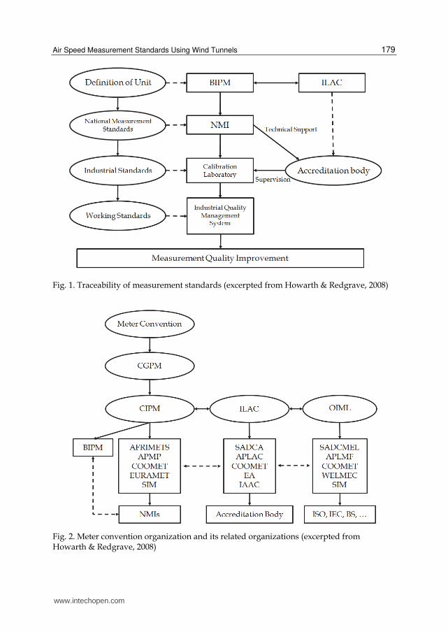
Fig. 1. Traceability of measurement standards (excerpted from Howarth & Redgrave, 2008)

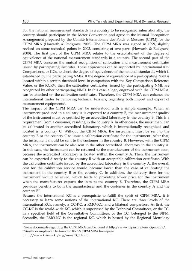
Fig. 2. Meter convention organization and its related organizations (excerpted from Howarth & Redgrave, 2008)

www.intechopen.com


For the national measurement standards in a country to be recognized internationally, the

country should participate in the Meter Convention and agree to the Mutual Recognition

Arrangement prepared by the Comité Internationale des Poids et Mesures (CIPM), or the

CIPM MRA (Howarth & Redgrave, 2008). The CIPM MRA was signed in 1999, slightly

revised on some technical points in 2003, consisting of two parts (Howarth & Redgrave,

2008). The first part of the CIPM MRA relates to the establishment of the degree of

equivalence of the national measurement standards in a country. The second part of the

CIPM MRA concerns the mutual recognition of calibration and measurement certificates

issued by participating institutes. These approaches can be supported by International Key

Comparisons, or KCs, to check the degree of equivalence of the national standards, which is

established by the participating NMIs. If the degree of equivalence of a participating NMI is

located within a certain threshold level in comparison with the Key Comparison Reference

Value, or the KCRV, then the calibration certificates, issued by the participating NMI, are

recognized by other participating NMIs. In this case, a logo, engraved with the CIPM MRA,

can be attached on the calibration certificates. Therefore, the CIPM MRA can enhance the

international trades by removing technical barriers, regarding both import and export of

measurement equipments6.

The impact of the CIPM MRA can be understood with a simple example. When an

instrument produced in a country A is exported to a country B, the measurement quality

of the instrument must be certified by an accredited laboratory in the country B. This is a

requirement from a customer, residing in the country B. In other cases, the instrument can

be calibrated in another accredited laboratory, which is internationally recognized and

located in a country C. Without the CIPM MRA, the instrument must be sent to the

country B or the country C to issue a calibration certificate for the instrument. After that,

the instrument should be sent to the customer in the country B. However, with the CIPM

MRA, the instrument can be also sent to the other accredited laboratory in the country A.

In this case, the instrument can be returned to the manufacturer of the instrument soon,

because the accredited laboratory is located within the country A. Then, the instrument

can be exported directly to the country B with an acceptable calibration certificate. With

the calibration certificate issued by the accredited laboratory in the country A, the overall

cost for the calibration service would become lower than the case of calibrating the

instrument in the country B or the country C. In addition, the delivery time for the

instrument would be saved, which leads to providing lower price for the instrument

when the manufacturer exports the item to the country B. Therefore, the CIPM MRA

provides benefits to both the manufacturer and the customer in the country A and the

country B7.

Because the international KC is a prerequisite to fulfill the spirit of CIPM MRA, it is necessary to learn some notions of the international KC. There are three levels of the international KCs, namely, a CC-KC, a RMO-KC, and a bilateral comparison. At first, the CC-KC is the world-wide KC, which is supervised by the Technical Committees, or the TC, in a specified field of the Consultative Committees, or the CC, belonged to the BIPM. Secondly, the RMO-KC is the regional KC, which is hosted by the Regional Metrology

6 Some documents regarding the CIPM MRA can be found at http://www.bipm.org/en/ cipm-mra/. 7 Similar examples can be found in KRISS CIPM MRA homepage (http://www.kriss.re.kr/eng/mra/03_1.html).

www.intechopen.com


Organizations, or the RMOs8. As in the CC-KC, the RMO-KC is supervised by the TC members, belonged to the RMO. Finally, the bilateral comparison is the international comparison to check the two independent national measurement standards, established at two participating NMIs. Any of these KCs should be reported to the RMOs or the BIPM to enroll their results to the BIPM database, or the KCDB9. To organize an international KC, a pilot laboratory, which leads the whole process of the

international KC, must prepare a test protocol that describes how the KC is to be

performed. The pilot laboratory provides an artifact or a transfer standard, and circulates

the artifact to the participating NMIs according to the test schedule. The purpose of the

artifact is to provide a guideline for estimating the degree of equivalence among the

national measurement standards established in the participating NMIs. As a circulation

scheme of the artifact, the round robin test is usually preferred; however, other circulation

schemes can be adopted, depending on the type of the KCs. After collecting all the

calibration data of the transfer standards with reference to the national measurement

standards of the participating NMIs, the pilot laboratory estimates the Key Comparison

Reference Value, or the KCRV. The degree of equivalence is then calculated by comparing

the calibration data given by the participating NMIs with the KCRV. In some cases, the

degree of equivalence is normalized within the range of (0 ~ 1). This is because sometimes

the normalized degree of equivalence is easier to be understood. When more than three

NMIs participate in the international KC, bilateral comparisons are also performed

because KCRVs for every two participating NMIs can be estimated. After summarizing

the results for the international KC, the pilot laboratory submits a draft report to the RMO

office. After suitable revisions are made according to the suggestions of the technical

committee members of the RMO, the draft report is approved as the final KC report, and

published in both the BIPM homepage and the Metrologia technical supplement (Terao et

al., 2007; Terao et al., 2010).

In view of traceability, the relationship between the CC-KC and the RMO-KC should be

linked via the KCRV, because the RMO- KC is smaller in scale than the CC-KC. To

establish linkage between the CC-KC and the RMO-KC, link laboratories, which have

participated in the CC-KC, participate also in the RMO-KC to bridge between the two KC

results. In this case, the same artifact, once used in the CC-KC, should be employed in the

subsequent RMO- KC. If there are any changes in the characteristics of the artifact due to

long-term stability, correction factors to the KCRV should be calculated. Toward this end,

a weighted average of the degree of equivalence among the link laboratories can be

considered to modify the KCRV in the RMO-KC, as an alternative method (Terao et al.,

2007; Terao et al., 2010).

3.2 Air speed metrology Air speed is a derived physical quantity, which is based on the mass measurement, according to the classification by the BIPM (Howarth & Redgrave, 2008). The Consulative Committee for Mass and related quantities, or the CCM, manages the physical quantities

8 In the RMOs, there are the APMP (Asia – Pacific region), the COOMET (East European – Siberian region), the EURAMET (European region), the SIM (North and South American region), and the AFRIMETS (African region). 9 The KCDB has a homepage at http://kcdb.bipm.org/

www.intechopen.com


such as mass, force, torque, pressure, density, viscosity, flow rate and flow velocity10. A sub-committe under the CCM, named as the Technical Comittee for Fluid Flow, or the TCFF, is in charge of the air speed metrology. The air speed metrology is classified into K3 category, therefore, the traceability for the air speed metrology is managed within the scope of the CCM.FF.K3. Hence, the CC-KC, regarding the air speed metrology, is termed as the CCM.FF.K3-KC. The first round of CCM.FF.K3-KC was held in 2005, and an ultrasonic anemometer was used as a transfer standard in the first round CC-KC (Terao et al., 2007). The reason, why the ultrasonic anemometer was used, was because the ultrasonic anemometer showed good measurement accuracy comparable with that of laser Doppler anemometers, which were established as primary standards in the participating NMIs. In the CC-KC, each participating NMI calibrated the ultrasonic anemometer (the 経戟劇) with the laser Doppler anemometer (the 迎継繋) in a wind tunnel (Terao et al., 2007). The role of the wind tunnel was to provide a testing environment to check both the repeatability and the reproducibility of the 経戟劇 and to provide calibration data for estimating the 計系迎撃 that was a crucial part of the KC.

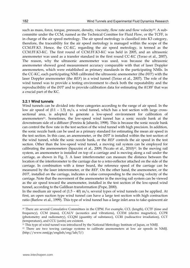
3.2.1 Wind tunnels Wind tunnels can be divided into three categories according to the range of air speed. In the low air speed of (0.1 – 1.5) m/s, a wind tunnel, which has a test section with large cross-sectional area, is adopted to generate a low-speed environment for calibration of anemometers11. Sometimes, the low-speed wind tunnel has a sonic nozzle bank at the downstream side of a diffuser (Pereira & Jabardo, 1998). This is because the sonic nozzle bank can control the flow rate in the test section of the wind tunnel with high precision. In addition, the sonic nozzle bank can be used as a primary standard for estimating the mean air speed in the test section. In this case, an anemometer, or the 経戟劇 is installed within the test section of the wind tunnel, while the sonic nozzle bank, or the 迎継繋 controls the air speed in the test section. Other than the low-speed wind tunnel, a moving rail system can be employed for calibrating the anemometers (Spazzini et al., 2009; Piccato et al., 2010)12. In the moving rail system, an anemometer is installed on top of a carriage and is moving along a rail under the carriage, as shown in Fig. 3. A laser interferometer can measure the distance between the location of the interferometer to the carriage due to a retro-reflector attached on the side of the carriage. In combination with a timer board, the reference speed of the carriage can be measured by the laser intererometer, or the 迎継繋. On the other hand, the anemometer, or the 経戟劇, installed on the carriage, indicates a value corresponding to the moving velocity of the carriage. Note that the movement of the anemometer in the moving rail system can be viewed as the air speed toward the anemometer, installed in the test section of the low-speed wind tunnel, according to the Galillean transformation (Pope, 2000). In the medium air speed of (1.5 – 40) m/s, several types of wind tunnels can be applied. At first, an open suction type wind tunnel can have a large test section with high contraction ratio (Barlow et al., 1999). This type of wind tunnel has a large inlet area to take quiescent air

10 There are several Consulative Committees in the CIPM. For example, CCL (length), CCTF (time and frequency), CCM (mass), CCAUV (acoustics and vibrations), CCEM (electro magnetics), CCPR (photometry and radiometry), CCQM (quantity of substance), CCRI (radioactive irradiation), CCT (temperature), and CCU (units) are existent. 11 This type of wind tunnel was introduced by the National Metrology Institute of Japan, or NMIJ. 12 There are two towing carriage systems to calibrate anemometers at low air speeds in NMIJ. (http://www.nmij.jp/english/org/lab/3/)

www.intechopen.com


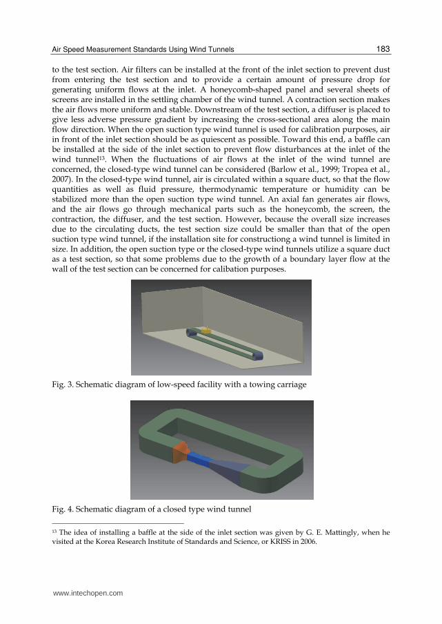
to the test section. Air filters can be installed at the front of the inlet section to prevent dust from entering the test section and to provide a certain amount of pressure drop for generating uniform flows at the inlet. A honeycomb-shaped panel and several sheets of screens are installed in the settling chamber of the wind tunnel. A contraction section makes the air flows more uniform and stable. Downstream of the test section, a diffuser is placed to give less adverse pressure gradient by increasing the cross-sectional area along the main flow direction. When the open suction type wind tunnel is used for calibration purposes, air in front of the inlet section should be as quiescent as possible. Toward this end, a baffle can be installed at the side of the inlet section to prevent flow disturbances at the inlet of the wind tunnel13. When the fluctuations of air flows at the inlet of the wind tunnel are concerned, the closed-type wind tunnel can be considered (Barlow et al., 1999; Tropea et al., 2007). In the closed-type wind tunnel, air is circulated within a square duct, so that the flow quantities as well as fluid pressure, thermodynamic temperature or humidity can be stabilized more than the open suction type wind tunnel. An axial fan generates air flows, and the air flows go through mechanical parts such as the honeycomb, the screen, the contraction, the diffuser, and the test section. However, because the overall size increases due to the circulating ducts, the test section size could be smaller than that of the open suction type wind tunnel, if the installation site for constructiong a wind tunnel is limited in size. In addition, the open suction type or the closed-type wind tunnels utilize a square duct as a test section, so that some problems due to the growth of a boundary layer flow at the wall of the test section can be concerned for calibation purposes.

Fig. 3. Schematic diagram of low-speed facility with a towing carriage

Fig. 4. Schematic diagram of a closed type wind tunnel

13 The idea of installing a baffle at the side of the inlet section was given by G. E. Mattingly, when he visited at the Korea Research Institute of Standards and Science, or KRISS in 2006.

www.intechopen.com


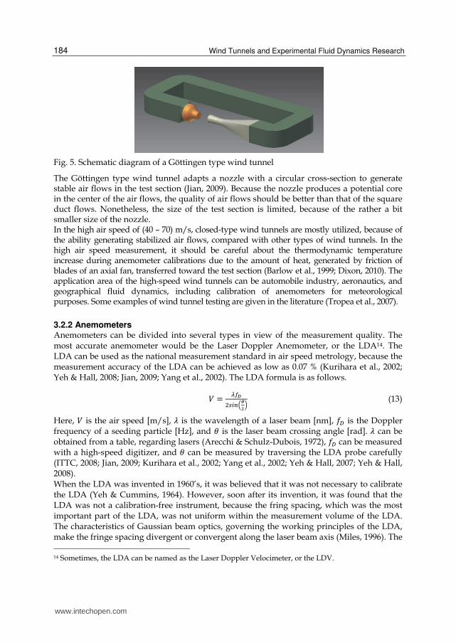
Fig. 5. Schematic diagram of a Göttingen type wind tunnel

The Göttingen type wind tunnel adapts a nozzle with a circular cross-section to generate stable air flows in the test section (Jian, 2009). Because the nozzle produces a potential core in the center of the air flows, the quality of air flows should be better than that of the square duct flows. Nonetheless, the size of the test section is limited, because of the rather a bit smaller size of the nozzle. In the high air speed of (40 – 70) m/s, closed-type wind tunnels are mostly utilized, because of the ability generating stabilized air flows, compared with other types of wind tunnels. In the high air speed measurement, it should be careful about the thermodynamic temperature increase during anemometer calibrations due to the amount of heat, generated by friction of blades of an axial fan, transferred toward the test section (Barlow et al., 1999; Dixon, 2010). The application area of the high-speed wind tunnels can be automobile industry, aeronautics, and geographical fluid dynamics, including calibration of anemometers for meteorological purposes. Some examples of wind tunnel testing are given in the literature (Tropea et al., 2007).

3.2.2 Anemometers Anemometers can be divided into several types in view of the measurement quality. The most accurate anemometer would be the Laser Doppler Anemometer, or the LDA14. The LDA can be used as the national measurement standard in air speed metrology, because the measurement accuracy of the LDA can be achieved as low as 0.07 % (Kurihara et al., 2002; Yeh & Hall, 2008; Jian, 2009; Yang et al., 2002). The LDA formula is as follows.

撃 = 碇捗呑態鎚沈津岾廃鉄峇 (13)

Here, 撃 is the air speed [m/s], 膏 is the wavelength of a laser beam [nm], 血帖 is the Doppler frequency of a seeding particle [Hz], and 肯 is the laser beam crossing angle [rad]. 膏 can be obtained from a table, regarding lasers (Arecchi & Schulz-Dubois, 1972), 血帖 can be measured with a high-speed digitizer, and 肯 can be measured by traversing the LDA probe carefully (ITTC, 2008; Jian, 2009; Kurihara et al., 2002; Yang et al., 2002; Yeh & Hall, 2007; Yeh & Hall, 2008). When the LDA was invented in 1960’s, it was believed that it was not necessary to calibrate the LDA (Yeh & Cummins, 1964). However, soon after its invention, it was found that the LDA was not a calibration-free instrument, because the fring spacing, which was the most important part of the LDA, was not uniform within the measurement volume of the LDA. The characteristics of Gaussian beam optics, governing the working principles of the LDA, make the fringe spacing divergent or convergent along the laser beam axis (Miles, 1996). The

14 Sometimes, the LDA can be named as the Laser Doppler Velocimeter, or the LDV.

www.intechopen.com


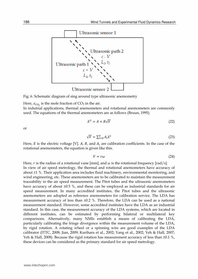
fringe distortion is because of the locations of two laser beam waists relative to the crossing point of the two laser beams. Therefore, an endeavor to align the laser beam waists is necessary to attain an ideal fringe divergence for the LDA (Yang et al., 2002). The ultrasonic anemometer can be used as a transfer standard because of high accuracy and good reproducibility (Terao et al., 2007; Terao et al., 2010). There are two kinds of measuring techniques to determine air speeds with the ultrasonic anemometers; One is the sing around and the other is the Doppler techniques. The sing around technique needs a pair of ultrasonic sensors to construct ultrasonic paths for measuring both the air speed and the speed of sound.

潔 + 撃 = 挑迭痛迭 (14)

潔 − 撃 = 挑鉄痛鉄 (15)

Here, 潔 is the speed of sound [m/s], 詣沈 (件 = 1, 2) is the path length between a pair of ultrasonic sensors (one is in the upstream direction and the other is in the downstream direction), and 建沈 (件 = 1, 2) is the transit time of ultrasonic waves from the transmitter to the receiver of the ultrasonic sensors. From Eqns. (14) and (15), the air speed and the speed of sound can be solved as follows.

潔 = 怠態岾挑迭痛迭 + 挑鉄痛鉄峇 (16)

撃 = 怠態岾挑迭痛迭 − 挑鉄痛鉄峇 (17)

Pitot tube can be also used as another transfer standard of air speed measurement, because the measured velocity by the Pitot tube is reliable (Blom et al., 2008). The working principle of the Pitot tibe is the Bernoulli equation for air speed and differential pressure between the total and the static pressure holes. The equation for the Pitot tube is as follows (ISO, 2008a; Tavoularis, 2005).

撃 = 岫な − 綱岻謬態綻牒諦 (18)

Here, (1-ε) is a compressibility correction factor, 貢 is the air density [kg/m3] and Δ鶏 is the differential pressure indicated by the Pitot tube [Pa]. The air compressibility can be expressed as follows (ISO, 2008a).

な − 綱 = 釆な − 怠態廷蔦椎諦 + 廷貸怠滞廷鉄岾蔦椎諦峇態挽怠/態 (19)

Here, 紘 is the ratio of specific heat capacities (潔蝶 and 潔牒). The air density can be expressed as follows (Picard et al., 2008).

貢 = 牒暢尼跳眺脹峙な − 捲塚岾な − 暢寧暢尼峇峩 (20)

Here, 鶏 is the atmospheric pressure [Pa], 警銚 is the molar mass of dry air [g/mol], 警塚 is the molar mass of water [g/mol], 捲塚 is the mole fraction of water vapour, 傑 is the

compressibility factor, 迎 is the molar gas constant [J/mol∙K], and 劇 is the thermodynamic

temperature [K]. If simplified by calculataions, Eqn. (20) becomes as follows.

貢 = 範ぬ.ねぱぬばねど + な.ねねねは ∙ 盤捲寵潮鉄 − ど.どどどね匪飯 ∙ 牒跳脹岫な − ど.ぬばぱど捲塚岻 (21)

www.intechopen.com


Fig. 6. Schematic diagram of sing around type ultrasonic anemometry

Here, 捲寵潮鉄 is the mole fraction of CO2 in the air.

In indutrial applications, thermal anemometers and rotational anemometers are commonly used. The equations of the thermal anemometers are as follows (Bruun, 1995).

継態 = 畦 + 稽√撃 (22)

or

√撃 = ∑ 畦沈継沈替沈退待 (23)

Here, 継 is the electric voltage [V]. 畦, 稽, and 畦沈 are calibration coefficients. In the case of the rotational anemometers, the equation is given like this.

撃 = 堅降 (24)

Here, 堅 is the radius of a rotational vane [mm], and 降 is the rotational frequency [rad/s]. In view of air speed metrology, the thermal and rotational anemometers have accuracy of

about ±1 %. Their application area includes fluid machinery, environmental monitoring, and wind engineering, etc. These anemometers are to be calibrated to maintain the measurement traceability in the air speed measurement. The Pitot tubes and the ultrasonic anemometers

have accuracy of about ±0.5 %, and these can be employed as industrial standards for air speed measurement. In many accredited institutes, the Pitot tubes and the ultrasonic anemometers are adopted as reference anemometers for calibration service. The LDA has

measurement accuracy of less than ±0.2 %. Therefore, the LDA can be used as a national measurement standard. However, some accredited institutes have the LDA as an industrial standard. In this case, the measurement accuracy of the LDA systems, which are located in different institutes, can be estimated by performing bilateral or multilateral key comparisons. Alternatively, many NMIs establish a means of calibrating the LDA, particularly calibrating the fringe divergence within the measurement volume of the LDA, by rigid rotation. A rotating wheel or a spinning wire are good examples of the LDA calibrator (ITTC, 2008; Jian, 2009; Kurihara et al., 2002; Yang et al., 2002; Yeh & Hall, 2007;

Yeh & Hall, 2008). Because the rigid rotation has measurement accuracy of less than ±0.1 %, these devices can be considered as the primary standard for air speed metrology.

www.intechopen.com


Anemometer Uncertainty factors

LDA beam crossing angle, Doppler frequency, fringe divergence, wavelength

Ultrasonic sensor distance, sound speed, time measurement, …

Pitot tube air density, differential pressure, expansibility, sensor alignment, …

Thermal curve fitting uncertainty, temperature, voltage, …

Rotational sensor alignment, radial location of rotating parts, rotating speed, …

Table 2. Uncertainty factors for various types of anemometers.

3.2.3 Calibration of anemometers When the anemometers are calibrated with a reference anemometer, calibration coefficient 糠 can be determined by calculating the ratio between the two anemometers.

糠 = 蝶馴曇鈍蝶呑南畷 (25)

Here, 撃帖腸脹 is the air speed from the calibrated anemometer (経戟劇) [m/s], and 撃眺帳庁 is the air speed from the reference anemometer (迎継繋) [m/s]. In view of traceability, 糠 can be obtained successively and transferred to other types of anemometers with lower measurement accuracies. Therefore, 糠 can be represented as follows.

糠 = 蝶馴曇鈍蝶呑南畷迭蝶呑南畷迭蝶呑南畷鉄蝶呑南畷鉄蝶呑南畷典 … 蝶呑南畷韮貼迭蝶呑南畷韮 = 糠怠糠態糠戴 … 糠津 (26)

Here, 岶糠沈 , 件 = な,に, … , 券岼 means the calibration coefficients by subsequent comparison between two anemometers, according to the traceability chain. For example, 糠怠 can be a calibration coefficient between the spinning wire and the LDA, 糠態 can be another calibration coefficient between the LDA and the ultrasonic anemometer, and so on. In these sussessive measurements, the uncertainty can be estimated as a vector sum among the calibrated apparatuses.

戟 = 倦紐憲眺帳庁態 + 憲帖腸脹怠態 + 憲帖腸脹態態 + ⋯ + 憲帖腸脹津態 (27)

Here, 憲眺帳庁 is the standard uncertainty of the 迎継繋, and 岶憲帖腸脹沈 , 件 = な,に, … , 券岼 is the standard uncertainties of the 経戟劇. The coverage factor, 倦 is then calculated by estimating the effective degree of freedom 荒勅捗捗 as explained previously.

荒勅捗捗 = 岫腸/賃岻填祢馴曇鈍填盃馴曇鈍袋祢呑南畷迭填盃呑南畷迭袋祢呑南畷鉄填盃呑南畷鉄袋⋯袋袋祢呑南畷韮填盃呑南畷韮 (28)

Here, 荒眺帳庁 is the effective degree of freedom of the 迎継繋, and 岶荒帖腸脹沈 , 件 = な,に, … , 券岼 is the effective degrees of freedom of the 経戟劇.

3.2.4 Uncertainty estimation of anemometers There are three kinds of methods to estimate the uncertainty of anemometers. The first method is to use first-order partial differentiation of an equation to the specific type of the anemometer (Thomas & Finney, 1988). If the anemometer equation is written as follows,

検 = 血岫捲怠, 捲態, … , 捲津岻 (29)

www.intechopen.com


then the uncertainty can be estimated based on the first-order partial differentiations of 検.

憲岫検岻 = 釆岾擢捗擢掴迭峇態憲岫捲怠岻態 + 岾擢捗擢掴鉄峇態憲岫捲態岻態 + ⋯ + 岾擢捗擢掴韮峇態憲岫捲津岻態挽怠/態 (30)

Here, 項血/項捲沈 can be denoted as 潔沈, a sensitivity coefficient (BIPM, 1993). As an example, the uncertainty of the LDA can be estimated by partial differentiation of Eqn. (13).

憲岫撃岻 = 釆岾擢蝶擢碇峇態憲岫膏岻態 + 岾擢蝶擢捗呑峇態憲岫血帖岻態 + ⋯ + 岾擢蝶擢提峇態憲岫肯岻態挽怠/態 (31)

擢蝶擢碇 = 捗呑態鎚沈津岾廃鉄峇 (32)

擢蝶擢捗呑 = 碇態鎚沈津岾廃鉄峇 (33)

擢蝶擢提 = − 怠替碇捗呑頂墜鎚岾廃鉄峇磐鎚沈津岾廃鉄峇卑鉄 (34)

The second method is to differentiate the anemometer equation, as seen in the first method. However, in this case, an equation with multiplication is more appropriate, because all the calculation is done by relative ratios of each independent variable.

検 = 捲怠銚捲態長 … 捲沈貸怠椎捲沈槌捲沈袋怠追 … 捲津佃 (35)

The first-order partial differentiation of 件-th independent variable can be written as follows.

擢槻擢掴日 = 圏捲怠銚捲態長 … 捲沈貸怠椎捲沈槌貸怠捲沈袋怠追 … 捲津佃

(36)

If the Eqn. (36) is divided by the Eqn. (35), then the ratio of 擢槻擢掴日 to 検 is calculated as follows.

買熱買猫日槻 = 槌掴日 (37)

Therefore, the ratio of uncertainty of 検 can be represented as follows.

通岫槻岻槻 = 釆岾擢槻擢掴迭峇態岾通岫掴迭岻槻峇態 + 岾擢槻擢掴鉄峇態岾通岫掴鉄岻槻峇態 + ⋯ + 岾擢槻擢掴韮峇態岾通岫掴韮岻槻峇態挽怠/態

(38)

Further simplified,

通岫槻岻槻 = 釆岾銚掴迭峇態憲岫捲怠岻態 + 岾長掴鉄峇態憲岫捲態岻態 + ⋯ + 岾佃掴韮峇態憲岫捲津岻態挽怠/態

(39)

In case of the rotational anemometers, the uncertainty can be estimated referring to Eqn. (24).

通岫蝶岻蝶 = 釆岾怠追峇態憲岫堅岻態 + 岾怠摘峇態憲岫降岻態挽怠/態

(40)

www.intechopen.com


The third method is to use a simplified version of Monte-Carlo simulation (ISO, 2008b; Landau & Binder, 2005). An input variable is composed of a large number of data more than 1,000,000, according to the Gaussian random process. The input variables to the anemometer equation should be independent and uncorrelated, to ensure a rigorous simulation for uncertainty estimation15. The mean and the standard deviation of each input variable are used to scale a Gaussian random signal. After that, the output variable, or the measuring quantity, is estimated by calculating the equation with the input variables. An example to estimate the measurement uncertainty of the Pitot tube is given as follows.

(Example) Estimate the standard (or Type A) uncertainty of the Pitot tube by using a Monte-Carlo simulation. The mean values and the standard deviations of each input variable are listed as follows. The number of simulation is 1,000,000. Δ鶏 : mean value = 5 Pa, standard deviation = 0.05 Pa (or 1 %)

貢 : mean value = 1.18 kg/m3, standard deviation = 0.012 kg/m3 (or 1 %) 綱 : mean value = 0.00002, standard deviation = 2×10-7 (or 1 %)

(Solution) The uncertainty estimation can be performed by programming with MATLAB16. To generate three Gaussian random signals with 1,000,000 samples, the command can be written as follows.

[s1, s2, s3] = RandStream.create('mlfg6331_64', 'NumStreams', 3); r1=randn(s1, 1000000, 1); r2=randn(s2, 1000000, 1); r3=randn(s3, 1000000, 1);

To confirm the uncorrelated signals, correlation coefficients can be calculated in matrix form.

A = corrcoef([r1, r2, r3]);

To give the above-mentioned mean values and standard deviations, following commands can be written.

% For differential pressure

del _ P _ avg 5;

del _ P _ std 0.05;

del _ P del _ P _ avg del _ P _ std * r1;

% For airdensity

rho _ avg 1.18;

rho _ std 0.012;

rho rho _ avg rho _ std * r2;

% For expansibility coefficient

ep

=

=

= +

=

=

= +

silon _ avg 0.00002;

epsilon _ std 2E 7;

epsilon epsilon _ avg epsilon _ std * r3;

=

= −

= +

15 In the case of correlated input variables, there should be another assumptions to generate random signals, which can give cross-correlation coefficients among the input variables. However, the book chapter only focuses on the case of the uncorrelated input variables. 16 In this example, MATLAB (R2010b) was used to generate Gaussian random signals.

www.intechopen.com


To calculate the Pitot tube velocity, the following commands can be added.

% For Pitot tube velocity

V=(1-epsilon).*(2*del_P./rho).^0.5;

V_avg=mean(V);

V_std=std(V);

V_ratio=V_std/V_avg*100;

The rests are to look at the calculated results for uncertainty estimations.

sprintf('V: mean=%12.4e, std=%12.4e, ratio=%12.4e %%', V_avg, V_std, V_ratio) figure('Name','Pitot tube velocity','NumberTitle','off') subplot1 = subplot(4,1,1); box(subplot1,'on'); hold(subplot1,'all'); plot(del_P); ylabel('ΔP [Pa]'); subplot2 = subplot(4,1,2); box(subplot2,'on'); hold(subplot2,'all'); plot(rho); ylabel('ρ [kg/m3]'); subplot3 = subplot(4,1,3); box(subplot3,'on'); hold(subplot3,'all'); plot(epsilon); ylabel('ε'); subplot4 = subplot(4,1,4); box(subplot4,'on'); hold(subplot4,'all'); plot(V); ylabel('V [m/s]'); xlabel('number of realization');

Here are some results for estimating the standard deviation of 撃.

A = 1.0000 0.0008 -0.0004 0.0008 1.0000 0.0012 -0.0004 0.0012 1.0000 V [m/s]: mean = 2.9111e+000, std = 2.0741e-002, ratio = 7.1248e-001 %

Therefore, the mean and the standard deviation of 撃 are 2.91 m/s and 0.021 m/s,

respectively. The standard (or Type A) uncertainty of 撃 would be 待.待態怠√怠,待待待,待待待 = に.な × など貸泰

[m/s]17. From the matrix 畦, it is noticed that cross-correlation coefficients among 堅怠, 堅態, and 堅戴, are small enough to assume the uncorrelated random signals among Δ鶏, 貢, and 綱.

3.2.5 Uncertainty estimation of a calibration curve When a curve fitting formula is considered to give a customer an estimate of air speed correction, uncertainty that is based on least square methods should be included (Hibbert, 2006). In many cases, in graphing the calibration data, the reference quantity (迎継繋) is located in the horizontal axis, while the tested quantity (経戟劇) is drawn in the vertical axis. Assuming the homoscedacity, there is no variance in the 迎継繋, or the horizontal axis (Hibbert, 2006). However, when estimating the measurement uncertainty, variances of the 経戟劇 by 兼 measurements (reproducibility) premises the variance of the 迎継繋. Therefore, in this case, the variance of the 迎継繋 can be estimated by calculating the residual standard deviation (Hibbert, 2006). In case of a linear regression, the calibation curve can be defined as follows.

検博 = 欠賦 + 決侮捲̅ (41)

17 This standard uncertainty considers only the type A uncertainty, which is determined by measurements. The type B uncertainty, which can be obtained from tables, calibration certificates, etc., should be included to complete the uncertainty estimation.

www.intechopen.com


Fig. 7. An example of a simplified Monte Carlo simulation

Here, 欠賦 and 決侮 are calibration coefficients. 捲̅ and 検博 are mean values of 券-realizations, i.e., 岶捲沈 , 検沈 , 件 = な,に, … , 券岼. Then, the residual standard deviation, 嫌槻 can be calculated as follows

(Hibbert, 2006).

嫌槻 = 俵∑ 岾槻日貸盤銚賦掴日袋長侮匪峇鉄日津貸態 (42)

Then, the standard uncertainty can be derived from the following equation (Hibbert, 2006).

嫌掴賦轍 = 鎚熱長謬怠陳 + 怠津 + 岫槻轍貸槻博岻鉄長鉄 ∑ 岫掴日貸掴̅岻鉄日 (43)

Here, 検待 is the mean value of 兼 responses, at a single point of 検沈, and 捲賦待 is the estimate of 捲待 by using Eqn. (41). (兼 means the reproducibility, and 券 means the number of calibration points.)

4. International comparisons

4.1 CC-KC The international Key Comparison aims to compare the national measurement standards

among participating NMIs and to harmonize the measurement traceability for establishing

the MRA. The meaning of the Key Comparisons is like this; when a person holds a key to a

box, then other people should also have the same keys to open the box. This means that the

measurement uncertainty among the participating NMIs should be located within an

acceptable level so that the national measurement standards are recognized to be equal.

0 2 4 6 8 10

x 105

4.5

5

5.5

∆P

[P

a]

0 2 4 6 8 10

x 105

1.1

1.15

1.2

1.25

㎥ρ

[kg

/]

0 2 4 6 8 10

x 105

1.8

2

2.2x 10

-5

ε

0 2 4 6 8 10

x 105

2.8

3

3.2

number of realization

V [

m/s

]

www.intechopen.com


The first round of the CC-KC, which was an world-wide level, was performed from April to

December in 2005, and its final report was published in October 2007 (Terao et al., 2007).

Four NMIs, including NMIJ (Japan), NMi-VSL (Netherlands), NIST (USA), and PTB

(Germany), participated in the CC-KC. NMIJ was the pilot laboratory for the CC-KC. A

three-dimensional ultrasonic anemometer was used as a transfer standard to be calibrated in

a wind tunnel or a specially-designed circular duct using the LDA. The calibration results

were summarized with air speeds of 2 m/s and 20 m/s as a calibration coefficient, 捲沈, which

has the same meaning as 糠 in Eqn. (25). Repeatability was checked by measuring the air

speed for 60 s to report the averaged air speed at 2 m/s and 20 m/s. Reproducibility was

also checked by several sets of air speed data.

To obtain the KCRV, which can be established as a standard value to compare the national

measurement standards among the participating NMIs, a weighted average was used and a

chi-squared test was performed to validate the weighted average. According to the Cox

method, the weighted average was acceptable as the KCRV if the chi-squared test was passed

(Cox, 2002). When the chi-squared test was failed, another method such as the simplified Monte

Carlo simulation with 106 random samples should be tried (ISO, 2008b; Terao et al., 2007).

To harmonize the national measurement standards of the participating NMIs, the degree of

equivalence, 穴沈 was defined as follows (Terao et al., 2007).

穴沈 = 捲沈 − 捲眺帳庁 (44)

Here, 捲沈 is the calibration coefficient of 件-th participating NMI, and 捲眺帳庁 is the 計系迎撃. Another definition of the degree of equivalence was introduced to compare the two national measurement standards between two participating NMIs.

穴沈,珍 = 捲沈 − 捲珍 (45)

The standard uncertainties of 穴沈 and 穴沈,珍 can be determined by vector sums between 捲沈 and 捲眺帳庁, or between 捲沈 and 捲珍, as follows (Terao et al., 2007).

憲岫穴沈岻 = 紐憲岫捲沈岻態 + 憲岫捲眺帳庁岻態 (46)

憲盤穴沈,珍匪 = 謬憲岫捲沈岻態 + 憲盤捲珍匪態 (47)

The number of equivalence, or the normalized degree of equivalence can be derived as follows (Terao et al., 2010).

継券沈 = |鳥日|賃通岫鳥日岻 (48)

継券沈,珍 = 弁鳥日,乳弁賃通盤鳥日,乳匪 (49)

Here, 継券沈 is the number of equivalence for 穴沈, 継券沈,珍 is the number of equivalence for 穴沈,珍, and 倦 is the coverage factor. The role of the number of equivalence is to provide a guideline whether the national measurement standard of each participating NMI has an equivalence in comparison with the 計系迎撃 or other national measurement standards from other NMIs. If the value is less than 1, then it can be said that the national measurement standard has equivalence with those of other NMIs.

www.intechopen.com


4.2 RMO-KC An RMO-KC, named as the APMP.M.FF.K3-KC, was performed from February to December in 2009 to give a supporting evidence for fulfilling the spirit of MRA (Terao et al., 2010). In the APMP-KC, five air speeds of (2, 5, 10, 16, 20) m/s were tested, and two of the air speeds, i.e., 2 m/s and 20 m/s, were selected to link the results to those of the CC-KC. The participating laboratories in the APMP-KC were NMIJ (Japan), CMS/ITRI (Chinese Taipei), KRISS (Korea), NIST (USA), NMC A*STAR (Singapore), and VNIIM (Russia). NMIJ was the pilot laboratory. In addition, there were two link laboratories (NMIJ and NIST) to link the KC results to those of the CC-KC. For this purpose, the three-dimensional ultrasonic anemometer, which had been adopted in the CC-KC, was also chosen in the APMP-KC. To link between the APMP-KC and the CC-KC results, a weighted sum was calculated using the calibration data from the two link laboratories as in the following equations (Terao et al., 2010).

経 = ∑ 拳沈経沈沈 (50)

経沈 = 捲沈,寵寵暢 − 捲沈,凋牒暢牒 (51)

拳沈 = 迭祢日鉄迭祢灘謎内乍鉄袋迭祢灘内縄畷鉄 (52)

Here, 経沈 is the difference between the CC-KC and the APMP-KC results. 捲沈,寵寵暢 is the CC-KC

results of the link laboratories, and 捲沈,凋牒暢牒 is those of the APMP-KC. 拳沈 is a weighting

coefficient, which can be calculated from the standard uncertainties of the link laboratories. In particular, 憲朝暢彫徴 is the standard uncertainty of the NMIJ and 憲朝彫聴脹 is the standard

uncertainty, given by the NIST, respectively. Through these calculatons, the APMP-KC results could be linked to those of the CC-KC by modifying the APMP-KC results as follows (Terao et al., 2010).

捲沈嫗 = 捲沈,凋牒暢牒 + 経 (53)

Here, 捲沈,凋牒暢牒 is the APMP-KC result of 件-th participating NMI and 捲沈′ is its modified value.

With 捲沈′, the normalized degree of equivalence, or the number of equivalence, 継券沈 could be estimated to harmonize the national measurement standards among the patricipating NMIs. In 2008, another RMO-KC, named as Euromet.M.FF-K3 KC, was reported. The participating laboratories were NMi-VSL (Netherlands), CETIAT (France), DTI (Denmark), SFOMA (Swiss), PTB (Germany), TUMET (Turkey), University of Tartu (Estonia), LEI (Lituania), INTA (Spain), and MGC-CNR (Italy). NMi-VSL was the pilot laboratory. The Euromet-KC was rather a bit an independent Key Comparison, because the transfer standards used in the KC were different from those used in the CC-KC or the APMP-KC (Blom et al., 2008). A Pitot tube with an amplifier and a thermal anemometer were chosen in the Euromet-KC as two transfer standards. Several air speeds between 0.2 m/s and 4.5 m/s were tested, which was proned to low air speed range, compared with the air speed ranges in the CC-KC. There was no linkage between the Euramet-KC and the CC-KC, due to the different measurement ranges of air speeds. The KCRV was calculated from a weighted average as follows.

計系迎撃 = ∑ 猫日祢盤猫日匪鉄日∑ 迭祢盤猫日匪鉄日 (54)

www.intechopen.com


憲懲寵眺蝶 = 怠俵∑ 迭祢盤猫日匪鉄日 (55)

The chi-square test was performed to validate the KCRV, and the chi-square test was passed

in the Euramet-KC. With the calibration coefficient 捲沈, the degree of equivalence or the

number of equivalence could be estimated to harmonize the national measurement

standards among the patricipating NMIs.

5. Conclusion

To enhance international trades with low technical barriers, some common perceptions of

measurement standards are necessary. In the early stages of measurement standards,

definition of basic units was the most important issue. With technological advancements,

the re-definitions of the basic units based on the physical constants have been suggested to

increase the measurability of the international standards. Traceability chain was probably

the second issue to establish an industrial infrastructure with reliable measurement

standards. Mutual recognition arrangement could be the third issue to enhance the

economic acitivity by lowering technical barriers, such as calibration certificates. This was

supported by the traceability chain and the international key comparisons in view of

metrologists.

In air speed measurement, various types of anemometers, including the rigid body

rotation, the LDA, the ultrasonic anemometer, the Pitot tube, the thermal and the

rotational anemometers, consisted the hierachy of the traceability chain. Wind tunnels,

such as the open suction, the close, and the Göttingen type wind tunnels, were used to

generate a stable test environment for anemometer calibrations. Uncertainty estimation of

anemometers was performed in three ways; first-order partial differentiation, a modified

partial-differentiation with a multiplicative equation form, and a simplified Monte Carlo

simulation.

Finally, some aspects of the international key comparisons, regarding the air speed

measurement, was surveyed. In the key comparisons, the key comparison reference value

was educed from a weighted average, and validated using the chi-square test. In some cases,

a Monte Carlo simulation was applied to obtain a suitable reference value for the key

comparison. To link between two different key comparison results, link to the key

comparison reference value was discussed. Throughout the analysis on the key

comparisons, the degree of equivalence among the participating national metrology

institutes was validated and the analysis was used as a supporting evidence to fulfill the

embodiment of the mutual recognition arrangement.

6. Acknowledgement

The author is grateful to Mr. Kwang-Bock Lee and Dr. Yong-Moon Choi for their helpful

advices, regarding general directions and criticism in preparation for the book chapter. This

work was partially supported by Korea Institute of Energy Technology Evaluation and

Planning (KETEP), which belonged to the Ministry of Knowledge Economy in Korea (grant

funded with No. 2010T100100 356).

www.intechopen.com


7. References

Arecchi, F. T. & Schulz-Dubois, E. O. (1972). Laser Handbook, North-Holland, ISBN 0-720-40213-1, Amsterdam, Netherlands

Barlow, J. B.; Rae, Jr., W. H. & Pope, A. (1999). Low-Speed Wind Tunnel Testing, John Wiley & Sons, ISBN 0-471-55774-9, New York, USA

Beckwith, T. G.; Marangoni, R. D. & Lienhard, J. H. (1993). Mechanical Measurements, Addison-Wesley, ISBN 0-201-56947-7, New York, USA

Bendat, J. S. & Piersol, A. G. (2000). Random Data: Analysis & Measurement Procedures, John Wiley & Sons, ISBN 0-471-31733-0, New York, USA

BIPM; IEC IFCC; ISO; IUPAC; IUPAP & OIML (1993). Guide to the Expression of Uncertainty in Measurement, International Organization for Standardization, ISBN 92-67-10188-9, Geneva, Swiss

Cox, M. G. (2002). The Evaluation of Key Comparison Data, Metrologia, Vol.39, pp.589-595, ISSN 0026-1394

Blom, G.; Care, I.; Frederiksen, J.; Baumann, H; Mickan, B.; Cifti, V.; Jakobson, E.; Pedisius A.; Sanchez, J. & Spazzini, P. (2008). Euromet.M.FF-K3 Euromet Key Comparison for Airspeed Measurements, EUROMET Project No. 514

Bruun, H. H. (1995). Hot-Wire Anemometry: Principles and Signal Analysis, Oxford University Press, ISBN 978-0-19-856342-6, Oxford, U.K.

Dixon, S. L. & Hall, C. A. (2010). Fluid Mechanics and Thermodynamics of Turbomachinery, Butterworth-Heinemann, ISBN 1-856-17793-9, New York, USA

Dougherty, E. R. (1990). Probability and Statistics for the Engineering, Computing and Physical Sciences, Prentice-Hall, ISBN 0-13-715913-7, New Jersey, USA

Gläser, M.; Borys, M.; Ratschko, D. & Schwartz, R. (2010). Redefinition of the kilogram and the impact on its future dissemination. Metrologia, Vol.47, pp.419-428, ISSN 0026-1394

Hibbert, D. B. (2006). The Uncertainty of a Result from a Linear Calibration. The Analyst, Vol.131, pp.1273-1278, ISSN 0003-2654

Howarth, P. & Redgrave, F. (2008). Metrology – In Short, EURAMET, ISBN 978-87-988154-5-7, Albertslund, Denmark

ISO (2005). General requirements for the competence of testing and calibration laboratories, International Organization for Standardization, ISO /IEC17025:2005, Geneva, Swiss

ISO (2008a). Measurement of Fluid Flow in Closed Conduits – Velocity Area Method Using Pitot Static Tubes, International Organization for Standardization, ISO 3966:2008, Geneva, Swiss

ISO (2008b). Propagation of distributions using a Monte Carlo method, International Organization for Standardization, ISO/IEC Guide 98-3:2008/Suppl 1:2008, Geneva, Swiss

ITTC (2008). Uncertainty Analysis: Laser Doppler Velocimetry Calibration, ITTC Recommended Procedures and Guidelines, International Towing Tank Conference, 7.5-01-03-02

Jian, W. (2009). Realization of a Primary Air Velocity Standard Using Laser Doppler Anemometer and Precision Wind Tunnel, XIX IMEKO World Congress, Fundamental and Applied Metrology, September 6-11, 2009, Lisbon, Portugal

Kirkup, L. & Frenkel, B. (2006). An Introduction to Uncertainty in Measurement Using the Gum, Cambridge University Press, ISBN 0-521-60579-2, New York, USA

www.intechopen.com


Kurihara, N.; Terao, Y. & Takamoto, M. (2002). LDV Calibrator for the Air Speed Standard between 1.3 to 40 m/s, Paper No. 61, 5th International Symposium on Fluid Flow Measurement, April, 2002, Arlington, Virginia, USA

Landau, D. P. & Binder, K. (2005). A Guide to Monte Carlo Simulations in Statistical Physics, ISBN 978-0-52-184238-9, New York, USA

Miles, P. C. (1996) Geometry of the Fringe Field Formed in the Intersection of Two Gaussian Beams, Applied Optics, Vol.35, No.30, pp.5887-5895, ISSN 0003-6935

Pereira, M. T. & Jabardo, P. J. S. (1998). A Wind Tunnel to Calibrate Probes at Low Velocities, Proceedings of FLOMEKO’98 9th International Conference on Flow Measurement, pp. 65-70, ISBN 91-630-6991-1, Lund, Sweden, June 15-17, 1998

Pope, S. B. (2000). Turbulent Flows, Cambridge University Press, ISBN 0-521-59886-9, Cambridge, U.K.

Piccato, A.; Malvano, R. & Spazzini, P. G. (2010). Metrological features of the rotating low-speed anemometer calibration facility at INRIM, Metrologia, Vol.47, pp.47-57, ISSN 0026-1394

Spazzini, P. G.; Piccato, A. & Malvano, R. (2009). Metrological features of the linear low-speed anemometer calibration facility at INRIM, Metrologia, Vol.46, pp.109-118, ISSN 0026-1394

Tavoularis, S. (2005). Measurement in Fluid Mechanics, Cambridge University Press, ISBN 978-0-52-181518-5, New York, USA

Terao, Y.; van der Beek, M.; Yeh, T. T. & Müller, H. (2007). Final Report on the CIPM Air Speed Key Comparison (CCM.FF-K3). Metrologia, Vol.44, Tech. Suppl., 07009, ISSN 0026-1394

Terao, Y.; Choi, Y. M.; Gutkin, M.; Jian, W.; Shinder, I. & Yang, C.-T. (2010). Final Report on the APMP Air Speed Key Comparison (APMP.M.FF-K3). Metrologia, Vol.47, Tech. Suppl., 07012, ISSN 0026-1394

Thomas, G. B. & Finney, R. L. (1988). Calculus and Analytic Geometry, ISBN 0-201-17069-8, Addison-Wesley, New York, USA

Tropea, C.; Yarin, A. L. & Foss, J. F. (2007). Handbook of Experimental Fluid Mechanics, Springer, ISBN 978-354-025141-5, Heidelberg, Germany

Yang, C. –T.; Wu, M. –C. & Chuang, H. –S. (2002). Adjustment and Evaluation of an LDA Probe for Accurate Flow Measurement, Optics and Lasers in Engineering, Vol.38, pp.291-304, ISSN 0143-8166

Yeh, T. T. & Hall, J. M. (2007). An Uncertainty Analysis of the NIST Airspeed Standards, ASME Paper FEDSM2007-37560, 5th Joint ASME/JSME Fluids Engineering Conference, July 30 - August 2, 2007, San Diego, California, USA

Yeh, T. T. & Hall, J. M. (2008). Uncertainty of NIST Airspeed Calibrations, Technical document of Fluid Flow Group, NIST, Gaithersburg, Maryland, USA

Yeh, Y. & Cummins, H. Z. (1964). Localized Fluid Flow Measurements with a He-Ne Laser Spectrometer, Applied Physics Letters, Vol.4, pp.176-178, ISSN 0003-6951

www.intechopen.com

Wind Tunnels and Experimental Fluid Dynamics ResearchEdited by Prof. Jorge Colman Lerner

ISBN 978-953-307-623-2Hard cover, 709 pagesPublisher InTechPublished online 27, July, 2011Published in print edition July, 2011

InTech EuropeUniversity Campus STeP Ri Slavka Krautzeka 83/A 51000 Rijeka, Croatia Phone: +385 (51) 770 447 Fax: +385 (51) 686 166www.intechopen.com

InTech ChinaUnit 405, Office Block, Hotel Equatorial Shanghai No.65, Yan An Road (West), Shanghai, 200040, China

Phone: +86-21-62489820 Fax: +86-21-62489821

The book â€œWind Tunnels and Experimental Fluid Dynamics Researchâ€ is comprised of 33 chaptersdivided in five sections. The first 12 chapters discuss wind tunnel facilities and experiments in incompressibleflow, while the next seven chapters deal with building dynamics, flow control and fluid mechanics. Third sectionof the book is dedicated to chapters discussing aerodynamic field measurements and real full scale analysis(chapters 20-22). Chapters in the last two sections deal with turbulent structure analysis (chapters 23-25) andwind tunnels in compressible flow (chapters 26-33). Contributions from a large number of international expertsmake this publication a highly valuable resource in wind tunnels and fluid dynamics field of research.

How to referenceIn order to correctly reference this scholarly work, feel free to copy and paste the following:

Sejong Chun (2011). Air Speed Measurement Standards Using Wind Tunnels, Wind Tunnels and ExperimentalFluid Dynamics Research, Prof. Jorge Colman Lerner (Ed.), ISBN: 978-953-307-623-2, InTech, Available from:http://www.intechopen.com/books/wind-tunnels-and-experimental-fluid-dynamics-research/air-speed-measurement-standards-using-wind-tunnels

© 2011 The Author(s). Licensee IntechOpen. This chapter is distributedunder the terms of the Creative Commons Attribution-NonCommercial-ShareAlike-3.0 License, which permits use, distribution and reproduction fornon-commercial purposes, provided the original is properly cited andderivative works building on this content are distributed under the samelicense.

https://creativecommons.org/licenses/by-nc-sa/3.0/

air speed measurement standards using wind tunnels

Documents