a 00

6 Z

.

t

C.P. No. 847

MINISTRY OF AVIATION

AERONAUTICAL RESEARCH COUNCIL

CURRENT PAPERS

Measurement of Turbulence in the

Liverpool University Turbomachinery

Wind Tunnels and Compressor

BY

R. Shaw, AK. Lewkowicz und J.P. Gostelow

LONDON: HER MAJESTY’S STATIONERY OFFICE

1966

SIX SHILLINGS NET’

C.P. No. 847

December, 1964

Measurement of Turbulence in the Liverpool University Turbomachinery Wind Tunnels and Compressor

- By - R. Shaw, A. K. Lewkowioz and J. P. Gostelow

Communicated by Prof. J. H. Horlook

SUMMARY

The measurement of the turbulenoe intensity in three wind tunnels and a research compressor is described and the minimum values are found to be 0*401$ for the No. 1 tunnel, 0.256% for the No. 2 tunnel, 0*36% for the boundary layer tunnel and 2*19$ for the compressor. It was found that the effect of the upstream gauze was critical.

Results for the tunnels and compressor after installation in a new building confirmed the above values for the tunnels, but indicated 1% turbulence intensity at inlet to the compressor due to the improved return air path in the new laboratory.

The turbulenoe titensities created by three different turbulence gias were measured.

-2-

1. Introduction

The turbulence of the free stream has a major effect on the flows that occur in turbomachinery. This is mainly due to the influence of the free-stream turbulence on the transition from laminar to turbulent boundary layer, its further development and hence its separation. Furthermore the boundary-layer performance interacts mth the free-stream flow and thus alters the conditions that would be expected from potential flow theory, In the Liverpool University Turbomachinery Laboratory various aspects of the flow in turbomachines have been investigated by means of a low-speed axial flow compressor and three different lovr-speed wind tunnels. These were subjected to turbulence tests and results with a limited discussion are given in the present report.

The nature of turbulence in a wind tunnel of conventional design, i.e., with proper settling chamber containing screens of honeycombs and gauzes plus an aerodynamically designed contraction can be expected to be homogeneous and nearly isotropic,.Schlichting,l. Townsend7 states that the flow dovrnstream of a uniform grid placed across the entrance to a wind4unnel working section, which is the experimental approximation to isotropic homogeneous turbulence, is not a homogeneous flow but a stationary one with an intensity gradient in the direction of mean flow. Theoretical isotropic turbulence, on the other hand, is homogeneous but not stationary in time, but under ordinary conditions the differences between the flows are slight. Therefore at a certain distance from the screens mean square velocity fluctuations in the three co-ordinate directions are assumed to be equal to each other.

In such cases the turbulence level, degree or intensity can be described by the quantity:-

G J&z?4 -= x 100 (%I . . . (I) U u

where U is a mean velocity.

The turbulence level is a very important parameter in wind-tunnel technique since it indicates the degree to which experiments in different tunnels can be compared as well as how measurements performed on a model can be applied to its full-scale version.

In the case of an axial flow compressor,owing to the complexity of the flow,one can hardly expect any isotropy or even homogenei@of turbulence. Nevertheless some measurements were conducted on the Liverpool University low-speed axial flow compressor in order to determine the influence of design and performance factors on the turbulence intensity in the axial and radial directions at several points inside the compressor. However, it should be emphasised that due to the reasons mentioned above any comparison of the compressor results with those obtained on the wind tunnels may have only limltedval~tity.

-3-

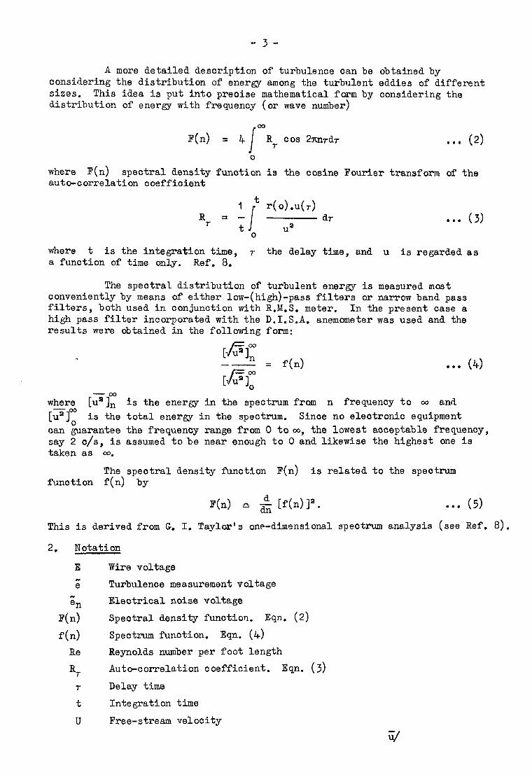
A more detailed description of turbulence can be obtained by considering the distribution of energy among the turbulent eddies of different sizes. This idea is put into precise mathematical form by considering the distribution of energy with frequency (or wave number)

i

cm F(n) = 4 BT cos 2xnrdr . . . (2)

0

where F(n) spectral density function is the cosine Fourier transform of the auto-correlation coefficient

I t r(o>.u(T> RT =t -

i a7

to ua l ** (3)

where t is the integration time, 7 the delay time, and u is regarded as a function of time only. Ref. 8.

The spectral distribution of turbulent energy is measured most conveniently by means of either low-(high)-pass filters or narrow band pass filters, both used in conjunction with R.M.S. meter. In the present case a high pass filter incorporated with the D.I.S.A. anemometer was used and the results were obtained in the following form:

[&I; -- = f(n)

[AT]; . . . (4)

where [us]: is the energy in the spectrum from n frequency to CO and [F]: is the total energy in the spectrum. Since no electronic equipment can guarantee the frequency range from 0 to 00, the lowest acceptable frequency, say 2 c/s, is assumed to be near enough to 0 and likewise the highest one is taken as 00.

The spectral density function F(n) is related to the spectrum function f(n) -by

This is derived from G. I. Taylor's one-dimensional spectrum analysis (see Ref. 8).

2. Notation

E Wire voltage

z Turbulence measurement voltage

"en Electrical noise voltage

F(n) Spectral density function. Eqn. (2)

f(n) Spectrum function. Eqn. (4)

Be Reynolds number per foot length

RT Auto-correlation coefficient. Eqn. (3)

T Delay time

t Integration time

U Free-stream velocity

. . . (5)

-4-

u Mean velocity fluctuation in stream direction

v Mean velocity fluotuation perpendicular to above w Mean velocity fluctuation perpendicular to above two caponents

CX Axial air velocity

um Mean blade velocity.

3. ’ Description of the Hot Wire Apparatus

The single ohannel apparatus used for the present measurements was originally assembled at the Aerodynamics Division of the National Physical Laboratory. It consisted of:

u

DISA Constant Temperature Anemometer (a), osoilloscope b , Cambridge Slide Wire Potentiometer (c), Scale lamp galvanometer a , Weston normal oell (e), and acoumulator (f). The general layout of the apparatus is shown in Fig. 2, and some main units on plate 1. The DISA Constant Temperature Anemometer (Fig. 3) is a self-contained unit sufficient for measuring both mean and fluctuating velocity oomponents. However, the potentiometer and galvanometer were incorporated into the circuit for accurate measurement of the wire voltage E.

The above equipment uan be used for quantitative measurements of the following factors in a turbulent flow: mean flow velooity v, root-mean

square value of the fluotuating velocity I-- 3 (hence turbulence intensity) and the spectrum analysis of a single electrical signal. The DISA anemometer oontains a Wheatstone's bridge in which one arm is replaced by the hot wire probe, bridge DC voltage measurement unit, bridge AC voltage (RMS) measurement unit and square wave generator. The input to the amplifiers is taken from the galvanometer points of the Wheatstone's bridge containing the wire, amplified and fed back at the battery points as a change in heating current. It reduces the unbalance of the bridge. The bridge DC voltage proportional to the mean velocity u is prooessed by ohopper DC amplifier, AC amplifier and DC output amplifier. The thermo-junction type unit yields bridge AC root-mean-square voltage which takes signals through the AC amplifier from the battery points of the Wheatstone's bridge. The RMS AC voltage proportional to the fluctuating

velocity component J- ua oan not be measured by means of the oommercial RMS voltmeter, as they are inaccurate for nonsinusoidal waveforms. A set of high and low pass filters permit spectrum analysis. In order to cheek the dynamio performance, the DISA set has been provided with the square wave generator which, when used together with the oscillosoope, oan be applied to measure the approximate value of the time constant of the system,

Single wire probes for the measurement of normal velocity components were supplied by the National Physical Laboratory (see Ref. 9). In all cases tungsten wire probes were used, as shown in Fig. 2. Diameter and length of the wire along its working se&ion were approximately 0*00015" ma 0.02" respectively. It was found that the cold resistanoe of the probe varied for different probes between 3.62 ohms and 5.06 ohms. The resistance also changed by 0.2 ohms with the same probe from day to day. Suitably dhosen operating resistance (1'7 to 2 x oold resistance) ensured that the wires were not heated above 300°C thus preventing rapid oxidation of the tungsten wire.

4./

-5-

4* Operational Procedure

In all cases the hot wire probes were positioned in such a way that the wire was perpendicular to the main-stream direction. Care was taken to ensure that the probes were mounted rigidly with respect to either wind-tunnel structure or axial flow compressor casing. This was to avoid any possible vibrations of the probe support. After the probe had been connected to the main circuit in the normal way the following operational procedure was adopted in order to measure turbulence intensity and turbulence spectrum.

a. Electronic noise

At the beginning and the end of each test, with tunnel (compressor) off . and with no draughts on the wire the thermo-junction (RMS) reading was

taken. This reading represented the electronic noise Zn due to the internal properties of the apparatus. If the position of the pointer was not steady (indicating that draughts as well as the electronic noise were contributing) the lowest reading was accepted as en.

b. Cold and operating resistances

With tunnel (compressor) running at required speed and the instrument on "stand by" the wire cold resistance was measured by adjusting "wide scale" control until the V pointer was on the red mark. After setting the expected cold resistance (3.552) on the three decades panel the "push to measure resistance" button was pushed. If the pointer went off the red mark the cold resistance was adjusted. The operating resistance was obtained by multiplying the cold one by the factor 1*7to 2 and set on the three decades panel.

c. Wire voltage

The wire voltage E was measured in a normal way by means of the slide wire potentiometer and the scale lamp galvanometer after these had been standardised and the DISA anemometer had been switched to "operate".

d. RAG of the fluctuating voltage

With DISA anemometer still on "operate" meter range was set to 1000 and "push to measure turbulence" button was pressed. The meter switch was turned to lower ranges progressively to obtain maximum sensitivity without over-loading the thermojunction instrument. The reading was taken when the pointer was stationary.

e. Frequency spectrum

For the measurements (a) to (a) both high and low pass filters were set to "out" position. In order to obtain the frequency spectrum, the high pass filter switch was turned to the next position, i.e., 5 c/s and the procedure in above paragraph (d) repeated. The high pass filter switch was set to a series of values and the above procedure repeated in each case.

5./

- 6-

5. Description of Tested Wind Tunnels and Axial Flow Compressor

3.1 No. 1 Tunnel

This is a blower tunnel which is used with porous sidewall suction to obtain accurate two-dimensional cascade results. The K. Blackman No, 21 fan is driven by a 36 H.P. D.C. motor which has a rheostat speed controls Further control is provided by means of a butterfly valve situatedin the 21 in. diameter inlet auct . Diffusion from the fan is effected by means of a fabricated steel, vaned diffuser of 230 maximum included angle. The 7 ft square settling chamber is provided with a gauze (which will be referred to later) and a 6 in. long honeycomb,

The contraction to the 12 in. x 29 in. working section was aerodynam'cally designed by means of a transformation method due to Gibbings and

3 Lewkowicz . Both contraction and working section are of a ribbed plywood construction. The working section is specifically designed for fixed inlet angle use with a cascade of 6 in. chord and compressor blade profiles. An intrinsic feature is the provision for wall boundary-layer bleed-off, which is carried out by the following means:-

(a) slots in top and bottom walls just ahead of the end blades.

(b) slots in side walls upstream of the cascade.

(c) porous side walls to eliminate contraction effects in the cascade.

The slots are in all casea designed and positioned to give minimum interference to the free-stream flow. Porous aide-wall auction is through a stainless steel 28 x 450 mesh gauze.

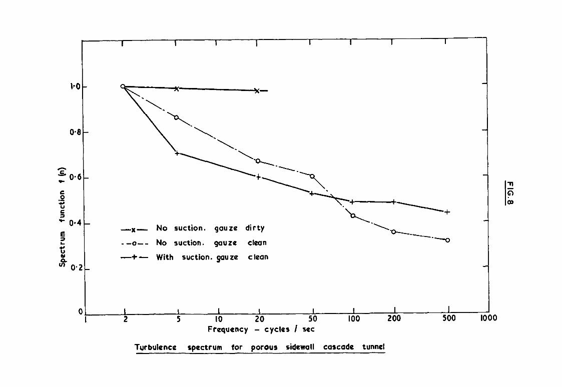
Two series of turbulence measurements were made in this tunnel. In the first series, although the precaution3 of scrupulou3ly cleaning the laboratory and sealing all the windows were taken, the gauze used in the settling chamber was frayed and dirty. The hot wire probe was positioned, on a rigid, cantilever, facing directly into the flow 2 f't upstream of the cascade. The free-stream turbulence intensity was found to have a minimum value of 206%.

A new phosphor bronze gauze of 40 x 40 mesh was installed especially for the second series of turbulence measurements and was securely fixed. The probe in this instance was positioned downstream of the cascade, well away from the blade wakes or wall boundary layers. The results of this teat are shown in Fig, 8; the order of the turbulence intensity having been reduced by a factor of 6,

5.2 No. 2 Cascade Tunnel

This tunnel, with a higher flow rate than the No, 1 tunnel, is mainly used to study the effect of aspect ratio and incidence variation on cascades. The fan used was a Blackman No. 48 EK, which was driven at 365 rpm. by a 13 H.P. motor. The diffuser has included angles of II0 and 17.60 in vertical and horizontal planes respectively and also discharges into a 7 ft square settling chamber, which has gauzes and a honeycomb. The contraction was designed in a similar way to that of the No. 1 tunnel, and the working section is 29 in, square.

Boundary/

-7-

Boundary-layer bleed-off is provided only through slots in the top and bottom walls. Further details of this tunnel and the No. 1 tunnel are given in Ref. 4.

The first series of turbulence measurements in this tunnel was not repeated since it had been possible on the first occasion to give all gauzes a thorough clean. The turbulence measurements were made with the cascade removed and the probe positioned in the centre of the working section, facing upstream.

5.3 Wind tunnel No. 2

Low-speed wind tunnel No. 3 has been designed to investigate the turbulent boundary layer in three dimensions. As shown on Fig. 6, air is delivered to the settlin chamber by a 2-stage VAirscreyP" fan which is driven by a 20 H.P. D.C. (electric 7 motor. The maximum velocity obtainable in the

4 ft x 2 ft working section is slightly above 60 ft/sec. Speed control by means of a rheostat assures fairly precise adjustment. The fan outlet diffuser is directly connected to the rear wall of the settling chamber, which has cross section dimensions - 8 ft sq and total length 11 ft. An aerodynamically designed contraction with a 4 ft x 2 ft working section directs the air to a 4 ft long straight duct and then to a curved duct containing a perspex flat plate on which the turbulent boundary layer is generated.

The settling chamber screens consist of a fine conical gauze attached to the fan diffuser , perforated steel plate and fine and coarse honeycombs.

The hot wire probe was placed at two different positions: at the exit from the curved duct, 6 in. above the plate (position A) and inside the duct, close to the leading edge of the plate, approximately 4 in. above the surface (position B), In both positions the hot wire probe was located in the free-stream flow, away from the boundary-layer. One test was performed with a forced separation on the plate created by lowering the rear part of the plate, (approximately; in total length) 6 in. below the front part. In this case the hot wire probe was placed in position A, 6 in. below the top wall. The probe was always positioned in such a way that the wire itself was parallel to the plate and vertical to the flow. In all cases the probe was supported rigidly in a holder normally used for boundary-layer traverses. The probes were always fixed with respect to the wind-tunnel structure.

5*4 Description of the low-speed research compressor

The compressor is shown in Fig. 7. The rotor, which is 3 ft in diameter, and the stator, which has an outside diameter of 4 ft are fabricated in mild steel. The aluminium alloy blades have a constant section (lOC.!+,/30 C50), a chord of 3 in., pitch/chord ratio of I at the tip and are set to a stagger angle of 360. The inlet guide vanes have the same geometry but are set at -20.70 stagger angle.

The design speed of the compressor is 684 rev/min and the design mass flow rate is 32.6 lbm/sec, giving 5% reaction at the blade tip and a Reynolds number (based on relative inlet velocity and chord) of 2 x 105.

The rotor is located between self-aligning ball bearings (parts 22 ' and 23)o The drive shaft (part 8) is connected to the rotor shaft by means of a flexible coupling (part 9). The power input was obtained from a d.c. motor (part 24)viaV‘belts which passed through the diffuser, but is now obtained from an induction motor driving through a Heenan and Froude Dynamatic Coupling and "Powergrip" belting.

The/

-8-

The diffuser has an inner cone made in timber and plywood whilst the octagonal outer wall is made in timber and Masonite board. The throttle (part 21) consists of 20 gauge sheet steel covering a frame of mild steel rods.

To eliminate all possible upstream disturbances to the airflow the radial-to-axial intake shown in Fig. 7 was chosen. The profiles of this air intake are based on a modified two-dimensional potential flow analysis and the resultant three-dimensional form was constructed in a fibreglass reinforced Polyester resin.

Instrumentation is provided to record the following information at 5 equally spaced circumferential positions:-

(a) Intake static pressure (inner end outer ducts),

(b) Intake total pressure.

(c) Compressor inlet static pressure (inner and outer wall).

(d) Compressor outlet static pressure (inner and outer wall).

Speed is measured by a revolution counter. Pitot-static yawmeter traverses can be carried out behind each blade row over the full radial distance and over two blade pitches circumferentially. Static pressure tappings are provided at 24 positions around the blade profiles in each blade row at root, mean and tip sections. The pressures from the rotor blade are transmitted through a pressure transmission unit which employs rubber ring seals and a hollow shaft with internal pressure tubing.

For the purpose of the turbulence tests the hot wire probe was placed just below the horizontal joint flange, at the mean radius with the axis of the wire normal to the flow direction and normal to the radial direction, and in three axial positions -

(i) approximately 1 ft upstream of the I.G.V's (position A in Fig. 7)

(ii) approximately 18 in. downstream of the stator, (position B)

(iii) approximately 5 ft downstream of the stator and near the exit of the diffuser (position C).

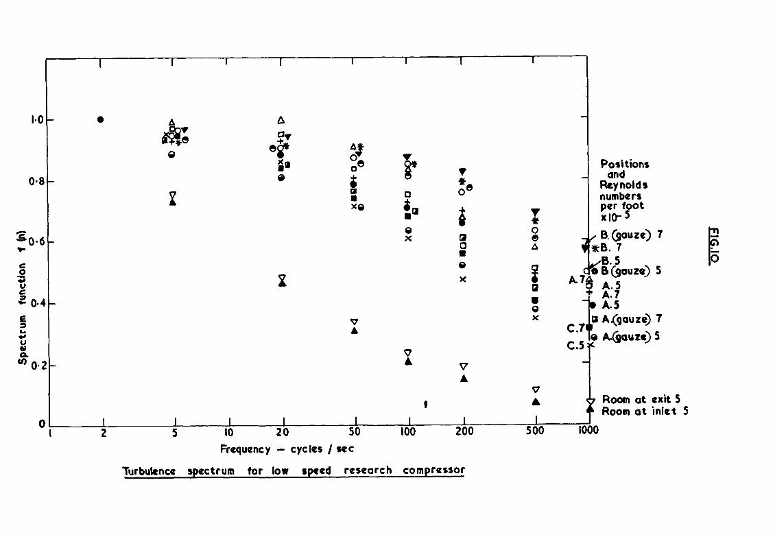
The restricted return air circuit in the room housing the compressor caused the compressor intake turbulence level to be high, so that some tests were also conducted in the air return space adjacent to the compressor. To reduce the intake turbulent eddy size a gauze was fitted over the air intake as shown in Fig. 7 and a further set of results obtained.

The results for turbulence intensity in the axial and radial direction, and a plot of the turbulence spectra is shown on Fig. IO.

6.1 Discussion of results. No. 1 Tunnel (see Table 7)

In the absence of any other factors which may have influenced the turbulence level, it is thought that the abrupt reduction was almost entirely

due/

-9 -

due to the state of the settling chamber gauze. This conclusion is supported by a comparison of the frequency spectra for the two series of tests. (Fig. 8). The limited spectrum taken with the old gauze in position reveals a very high frequency turbulence of the type that one would expect to be generated by dust particles on the gauze. The spectra for the second series of tests are of the more usual pattern, with a sizeable low frequency component.

6.2 Discussion of results. No. 2 Tunnel

No definite trend is discernible from the results, the turbulence level varying very little over the range of operating speeds. Since the gauzes were clean at the time of test, and are normally maintained in that state, and since there are no porous side walls, no further variables were taken into account.

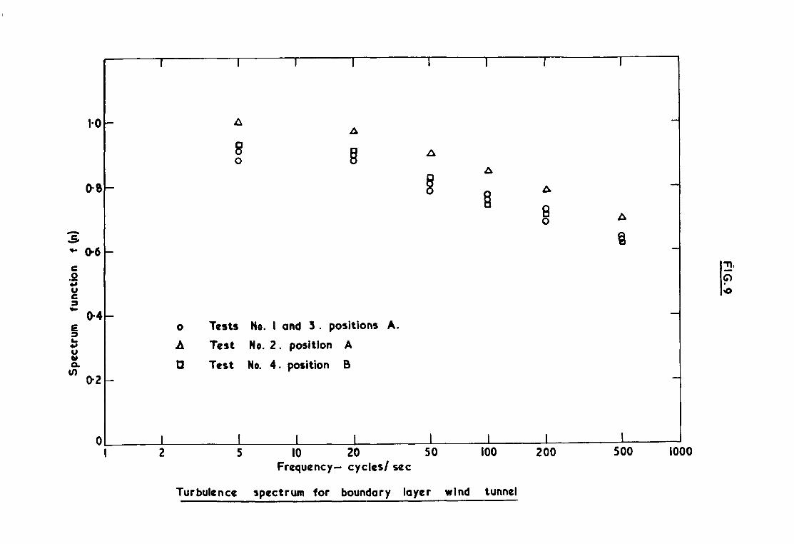
6.3 Discussion of results. No. 3 Tunnel

Tests were carried out in two different positions and in one case with forced separation due to a step in the plate. Results are presented for all the cases in Table 3 and the spectral distribution of turbulent energy is

represented by the factor [@I,"

on Fig. 9. As seen from the Table 3, and

Fig. 9, the turbulence intensity slightly increases towards the exit of the ' curved duct, however the spectral behaviour remains practically the same,, The

small. decrease in turbulence intensity in the exit section in case of the flow with forced separation (test No. 2) is probably due to an experimental error. The spectrum curve of the separated flow appears to tend to slightly higher values than others. However the differences are in general rather small,,

6.4 Discussion of Results. Compressor

Without the intake gauze the turbulence intensity in the axial and radial directions in the compressor is high (4% to %) and actually decreases slightly through the blade rows. This suggests that the turbulence in this case is due more to the unsteady flow in the return air circuit in the room than to turbulence generated in the compressor.

The apparent increase in turbulence at diffuser exit is mainly due to the reduction in the mean velocity component by a factor of two, so that 4g37-)

is thereby doubled. Similarly the excessively large turbulence u

intensity outside the compressor is due mainly to the low mean velocity component here (approximately l/30 the velocity in the compressor).

Observation of the unsteady flow in the return air circuit suggested a very low frequency turbulence, i.e., very large eddy size. The turbulence spectrum confirms this observation since high frequency turbulence is relatively small outside the compressor whilst the higher frequencies are relatively most significant immediately downstream of the stator row.

The/

- 10 -

The air intake causes a decrease in turbulence level due to the increase in the mean velocity and alters the spectrum so that excessive low frequency turbulence is reduced relative to the higher frequency turbulence.

The inclusion of an intake gauze reduces the turbulence intensity in axial and radial directions to about 2% upstream of the I.G.V's, primarily by reduction of the higher frequency components.

7. Conclusions

Tunnel No. 1. With clean settling chamber gauze and at a fixed Reynolds number of 4 x IO' per foot, the turbulence intensity varied from 0*4C$ with sidewall suction to 004% without suction.

When the gauze is dirty the turbulence intensity rises to the region

Tunnel No. 2. With clean settling chamber gauze and at Reynolds numbers from 3 x IO5 to 4 x ?05 per foot, the average turbulence intensity is 0'2% with no discernible Reynolds number variation.

Tunnel No. 2. intensity increases from the duct.

At a Reynolds number of 3.3 x IO' per foot the turbulence from 0 036% at entry to the curved duct to O*@$ at exit

w- Without an intake gauze and at Reynolds numbers of 5 x 106and 7x10 perfootthet bl ur u ence intensity in the axial and radial directions (upstream of the I.G.V's) is 4% to %. This reduces to about 2% when a gauze is fitted at the intake.

There is a high intensity of low frequency (atmospheric type) turbulence in the return air circuit in the room which should be significantly reduced when the compressor is moved to a more spacious laboratory in the near future.

The turbulence intensities recorded in the wind tunnels fall within the range of turbulence intensities quoted by Bradshaw and Ferris (Ref.2) for some low-speed tunnels at N.P.L., but are high in relation to the value of 0*02$ quoted by Schubauer and Skramstad (R'ef.5) for a specially designed low turbulence tunnel0 (National Bureau of Standards, Washington).

Since the turbulence in the worki.ng section of the windtunnels-can be expected to be homogeneous and nearly isotropic (Ref. 1) *then $ = 4 = ?

G and the simplified expression for turbulence intensity- x 10% is valid.

U This is not so in the compressor and the turbulenoe intensity quoted is the mean value for the axial and radial directions (the axis of the probe wire being perpendicular to these two directions).

- 11 -

a. Discussion of Additional Results and Conclusions

8.1 Tunnel NO. I

After rebuilding the tunnel in a new laboratozy the turbulence intensity was found to be 0*51% at a Reynolds number of 4 x I@ per ft (compared with 0*4% in the earlier tests), and was found to increase to 0064% at a Reynolds number of 2 x I@ per ft.

8.2 Tunnel No. 1 wfth turbulence grids

A turbulence grid consisting of 3 round bars at 36 in. pitch and located 6 in. upstream of the contraction throat created a turbulence intensity (just upstream of the cascade) of 2*1C$ at a Reynolds number of 4 x I@ per ft. This value changed only slightly for lower Reynolds numbers down to 2 x I@ per ft.

A turbulence grid consisting of 1 in. flat bars at 3 in. pitch and located at the contraction throat created a turbulence intensity of about 13% just upstream of the cascade at a Reynolds number of 4 x I@ per ft. There was a c!A$ variation depending on the position of the hot wire probe relative to the bars of the turbulence grid. The turbulence intensity just downstream of the cascade and between the blade wakes was 9'75%.

a.3 Tunnel No. 2

After rebuilding the tunnel in the new laboratory the turbulence intensity was found to be about 0'2% In the Reynolds number range per ft from 3 x I@ to 4 x I@, compared with the earlier value of about 0.2%.

8.4 Tunnel NO, 2 with turbulence grids

A turbulence grid consisting of $ in. round bars at 14 in. pitch located just upstream of the contraction throat produced a turbulence intensity of 0*9$, whilst the grid of 4 in. round bars created a turbulence intensity of 1.6% and the grid of 1 in. flat bars created about lO*OC$ turbulence intensity.

a.5 Tunnel No. 3

At a Reynolds nmber of 3.3 x Id the turbulence intensity was found to increase from O-l% at entry to the curved duct to 0*2&$ at exit from the duct (compared with 003% and 00% respectively in the earlier tests). This reduction can be explained by the inclusion of an additional fine gauze in the settling length after the honeycombs. Two other changes have been made to this tunnel, namely the substitution of a new single stage fan and the removal of the intake oil filters, but these changes are not thought to have contributed significantly to the change of turbulence intensity.

8.6 Compressor

The compressor has now been rebuilt in a tich more spacious laboratory which allows a sufficiently large return air circuit for the elimination of the low frequency atmospheric type turbulence which had been associated with the intake air in the previous tests. As a result the turbulence intensity is now reduced to about I$ at compressor inlet with a small Reynolds number effect superimposed. This is a very significant reduction below the 4% to % previously measured.

Acknowledgements/

- 12 -

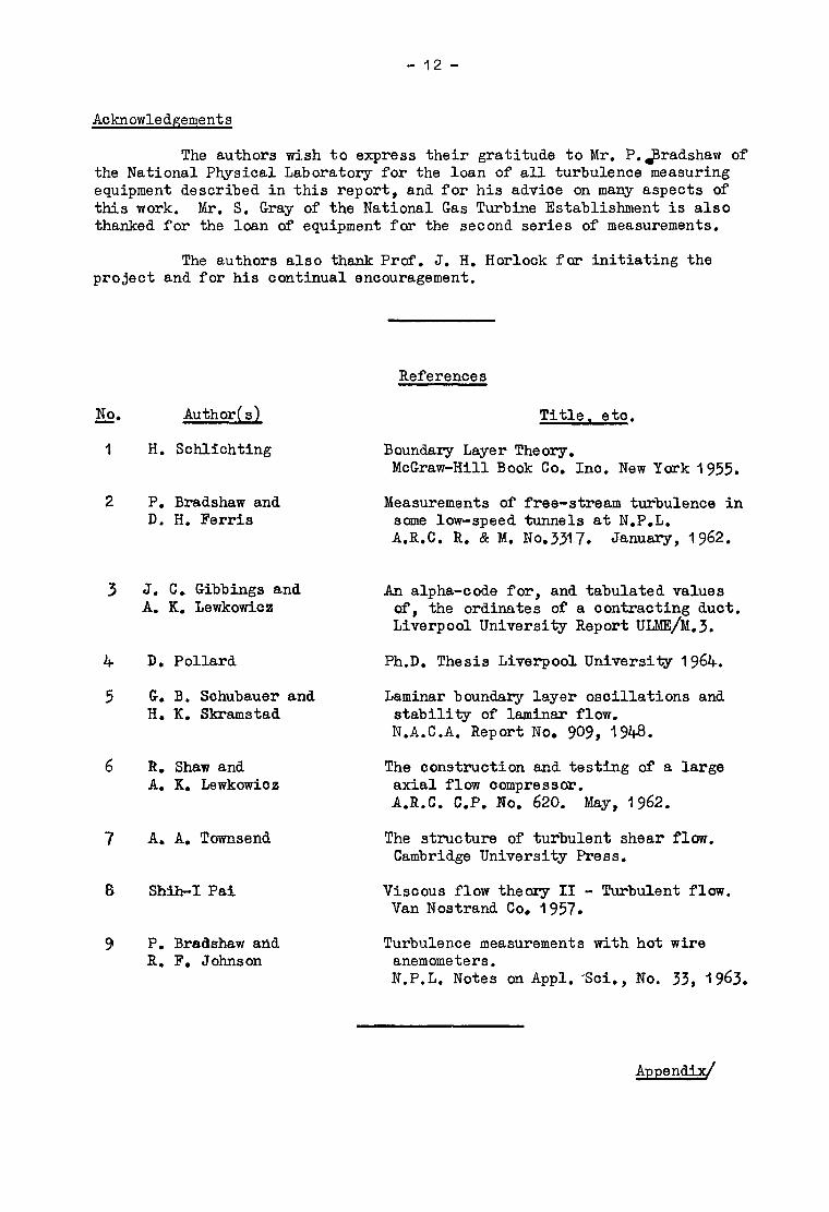
Acknowledgements

The authors wish to express their gratitude to Mr. P.$radshaw of the National Physical Laboratory for the loan of all turbulence measuring equipment described in this report, and for his advice on many aspects of this work. Mr. S. Gray of the National Gas Turbine Establishment is also thanked for the loan of equipment for the second series of measurements.

The authors also thank Prof. J. H. Horlock for initiating the project and for his continual encouragement.

3. Author(s)

1 H. Schlichting

2 P. Bradshaw and D. H. Ferris

3

4

5

6

J. C, Gibbings and A. K. Lewkowicz

D. Pollard Ph.D. Thesis Liverpool University 1964.

G. B. Schubauer and H. K. Skramstad

Laminar boundary layer oscillations and stability of laminsr flow. N.A.C.A. Report No. 909, 194.8.

R. Shaw and A. K. Lewkcwicz

A. A. Townsend

Shih-I Psi

P. Bradshaw and Turbulence measurements with hot wire R. F. Johnson anemometers.

N.P.L. Notes on Appl. 'Sci., No. 33, I 963.

References

Title, etc.

Boundary Layer Theory. McGraw-Hill Book Co. Inc. New York 1955.

Measurements of free-stream turbulence in some low-speed tunnels at N.P.L. A.R.C. R, & M. No.3317. January, 1962.

An alpha-code for, and tabulated values of, the ordinates of a contracting duct. Liverpool University Report ULME/M,3.

The construction and testing of a large axial flow compressor. A.R.C. C.P. NO. 620. May, 1962.

The structure of turbulent shear flow. Cambridge University Press.

Viscous flow theory II - Turbulent flow. Van Nostrand Co. 1957.

Appendix/

-13 -

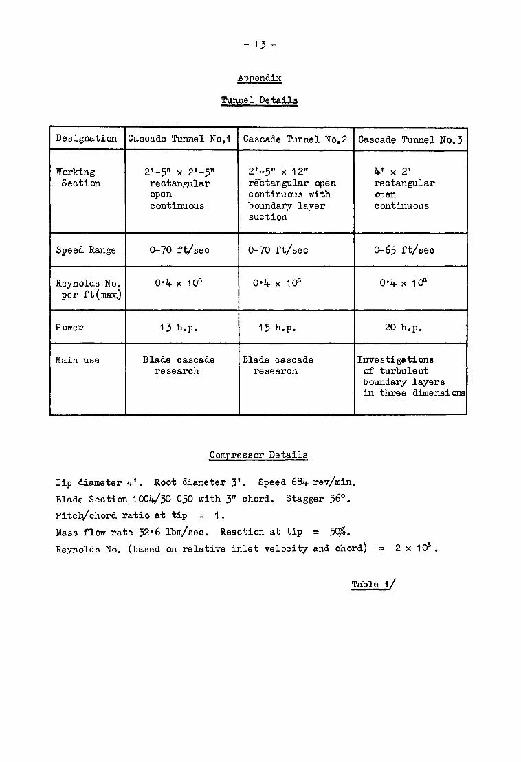
Appendix

Tunnel Details

Designation Cascade Tunnel No.1 Cascade Tunnel No.2 Cascade Tunnel No.3

Working 2'-5" x 21-5" 2*-5" x 12" 4’ x 2' Section rectangular rGtangular open rectangular

open continuous with open continuous boundary layer continuous

suction

Speed Range O-70 ft/sec O-70 ft/sec o-65 ft/sec

Reynolds No. 0*4 x IO6 o-4 x 106 0*4 x I@ per ft(max)

Power 13 h.p. 15 h.p. 20 h.p.

Main use Blade cascade Blade cascade Investigations researoh research of turbulent

boundary layers in three dimension

Compressor Details

Tip diameter 4'. Root diameter 3'. Speed 684 rev/min. Blade Section IO&/JO C50 with 3" chord. Stagger 36O. Pitch/chord ratio at tip = 1.

Mass flow rate 32.6 lbm/sec. Reaction at tip = 5%. Reynolds No. (based on relative inlet velocity and chord) 3: 2 x ld.

Table I/

- 14 -

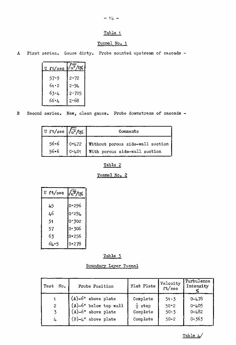
Table 1

Tunnel No. 1

A First series. Gauze dirty. Probe mounted upstream of cascade -

-.

B Second series. New, clean gauze. Probe downstream of cascade -

U ft/sec

t-

56.6

56-6

U ft/sec L-/q y 0

45 0-296

46 0.294

51 0.302

57 oa306

63 oa256

6405 0=278

Comments

0.472 Without porous side-wall suction

0*401 With porous side-wall suction

Table 2

Tunnel No. 2

3 Table

Boundary Layer Tunnel

I Test No. 1 2 r 3

4

Probe Position Flat Plate Velocity ft/sec

(A)-6" above plate Complete 51.3 0.478 (A)-6" below top wall & step 50-2 0*405 (A)-6" above plate Complete 50.3 0.482

(B)-4" above plate Complete 50-2 0.363

Table 4/

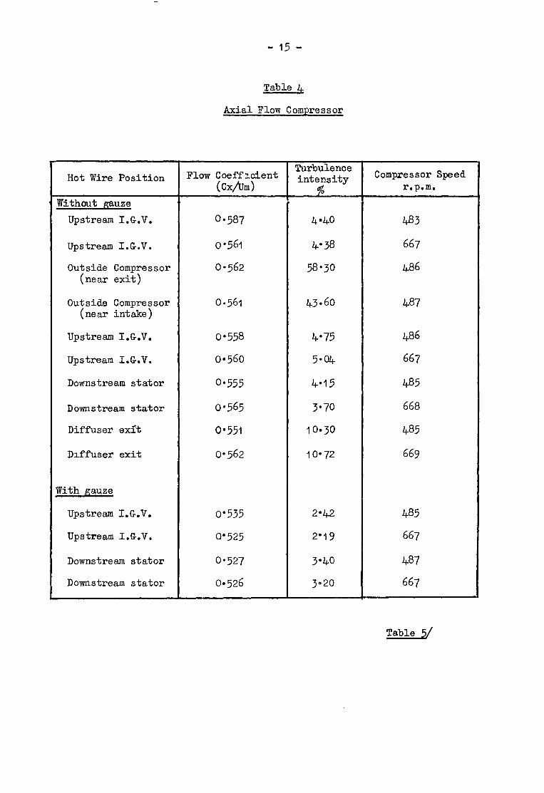
Hot Wire Position

Without gauze Upstream I.G.V.

Upstream I.G.V.

Outside Compressor (near exit)

Outside Compressor (near intake)

Upstream I.G.V.

Upstream I.G.V.

Downstream stator

Downstream stator

Diffuser edt

Dlff'user exit

With gauze

Upstream I.G.V.

Upstream I.G.V.

Downstream stator

Downstream stator

- 15 -

Table .+

Axial Flow Compressor

Flow Coefficient (CxbJm>

O-587 4*4o 483

0.561 4-38 667

0.562 58.30 486

09561 43.60 487

O-558 4*75 486

oa560 5.04 667

o-555 4*15 485

0*565 3.70 668

0.551 IO.30 485

o-562 IO-72 669

0.535 2.42 485

0.525 2'19 667

0.527 3-40 487

0.526 3020 667

Turbulence intensity

Table 5/

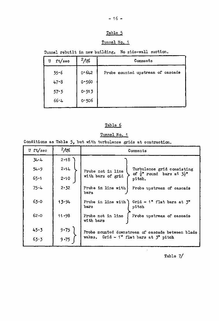
- 16 -

5 Table

Tunnel No. 1

Tunnel rebuilt in new building. No side-wall suction.

U ft/sec 2/% Comments

35*6 0-W Probe mounted upstream of cascade

47-0 0~560

57.5 O-513

66.4 0.506

Fable 6

Tunnel No. 1

Conditions as Table 5, but with turbulence grids at contraction.

U ft/sec

3494

54-Y

65a-1

75*4

2/%

2*18

2-14

2-10

2.32

Comments

Probe not in line Turbulence grid consisting of 1 with bars of grid 5" round bars at 36"

pitoh.

Probe in line with Probe upstream of cascade bars

63.0

62.0

13-94 Probe in line with Grid - 1" flat bars at 3" bars pitch

11998 Probe not in line Probe upstream of cascade with bars

45.3 Probe mounted downstream of cascade between blade

63-3 wakes. Grid - I‘" flat bars at 3" pitoh

Table '7/

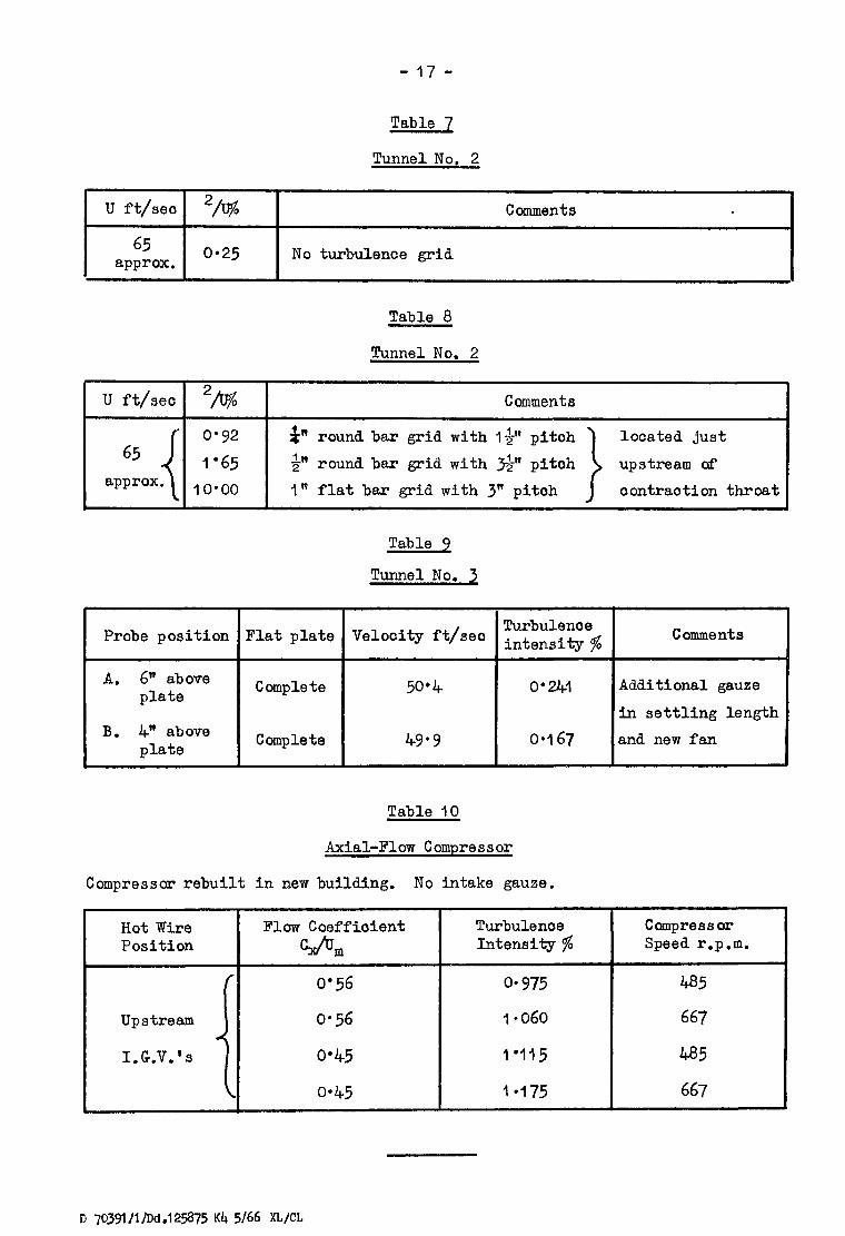
- 17 -

7 Table

Tunnel No, 2

u ft/sec 2/q

65 approx. 0.25 No turbulence grid

Comments

0.92

1'65 10'00

Probe position Flat plate

A. 6" above plate

B. 4" above plate

Table a

Tunnel No. 2

Comments

4" round bar grid with I$-" pitch located just $" round bar grid with 39 pitoh 1" flat bar grid with 3' pitoh oontraction throat

2 Table

Tunnel No. 2

Complete

Complete

Velocity f-t/sea

50.4

49*9

Turbulenoe intensity $

0'241

0.167

Table 10

Axial-Flow Compressor

Compressor rebuilt in new building. No intake gauze.

Hot Wire Flow Coeffioient Turbulenoe Position wrn Intensity $

i

0'56 0'56

Upstream Upstream 0.56 0.56

I.G.V.'s I.G.V.'s 0.45 0.45

O-4-5

Comments

Additional gauze

in settling length and new fan

Compressor Speed r.p.m.

0.975 485

I -060 667

I.115 435

l-475 667

D ~03~/1/od.l25&'5 K4 5166 XL/CL

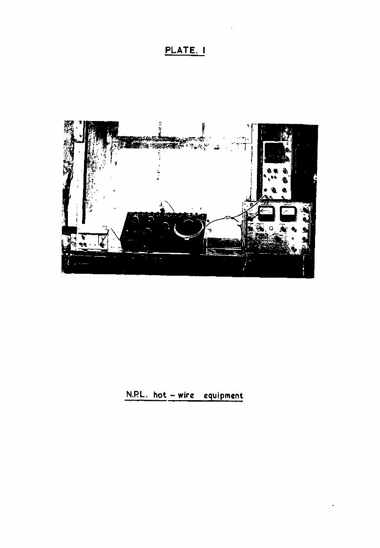
PLATE. I

N.PL. hot - wire equipment

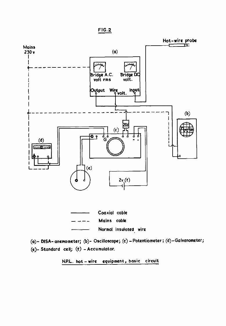
FIG.2

Mains

2iov I e-

-----------

I I I I I I

k_----- ------ -

(a)

volt rms volt.

Output WiNvolt In .

I I I \

L

I

we -m-m- - - - - - - - 1 I

(9

I

i I L4L

A I

d

Hot-wire probe -I u

Coaxial cable - --- Mains cable

Normal insulated wire

(a)- DISA- anemometer; (b)- Oscilloscope; (c) - Potentiometer ; cd)-Galvanometer;

(e)- Standard cell; (f) - Accumulator.

N.PL. hot - wire equipment, basic circuit

FIG. 3

Resistance mrasurement

-+

-1 I

i Off

WPlY

Hot-wire v probe

m

1 l W”

f

wave test

-Chopper r L RC. amplifie

D.C.output - amplifier -

- A.C. amplifier

d -z

OpProtc

Bridge

> D-C. voltage

Bridge A.C. voltage rms

A.C. ampllf ie r

Thermo- junction instrument

square wave 0 gmerator

Stand by Gesis tance measurefneti)

DISA 55 AOI hot - wire anemomr ter, block diagram

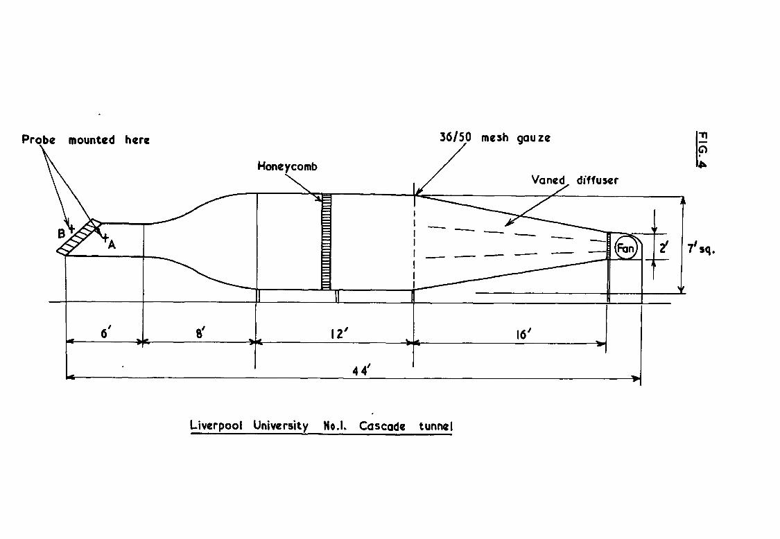
Pro,be mounted here

Honeycomb

36/50 mesh gauze

/ Vaned diffuser

--

--- --

Liverpool University No.1. Cascade tunnel

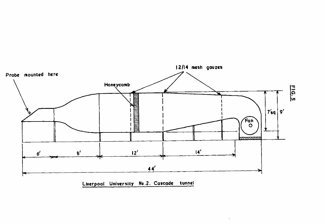
12114 mesh gauzes

Probe mounted here

I

I

I

I

I \T

6’ 0’ 12’ 14’ T

44’

Liverpool University No .2. Cascade tunnel

I

- I 11 F ul

9’

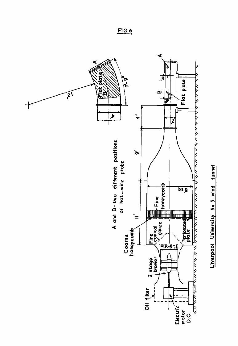
FIG.6

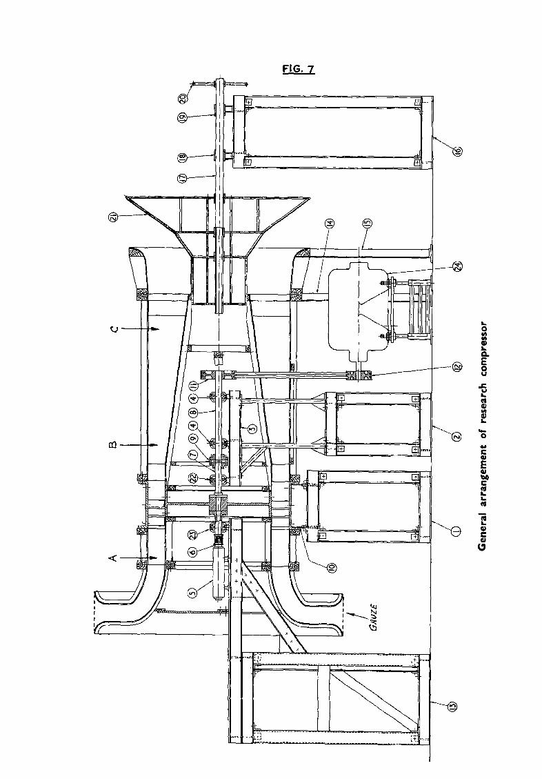
FIG. 7

-

0.8 -

= z 096-

c 0 .- t: I *- 0*4 -

5 ii x lo 0*2-

0, I

-x- No suction. gauze dirty

--u-w No suction. gauze clean

-+- With suction. gauze clean

I I I I I I I I

I 2

I 5

I I I IO 20 50

Frequency - cycles / set

I I I 100 200 500 1000

Turbulence spectrum for porous sidewall cascade tunnal

A

8 0

A

0 0 A

B

I I I I I I I I 5 IO 20 50 100 200 so0 1000

Frequency- cycles/ set

Tur bule n ce spectrum for boundary layer wind tunnel

0 Tests No. I and 3. positions A.

A Test No. 2. position A

b Test No. 4. position 8

1

X

v A

: 0

ad

8 u m 0 x

V A V

A v

1 A

I I I I I I I I 2 5 IO 20 so 100 200 500 I

Frequency - cycles / set

Turbuknce spectrum for low speed research compressor

p::fions Reynolds numbers per foot x10-*

B.@aute) 7 kB. 7

1 Room at exit 5 Room at inlrt S

m II

C.P. No. 847

0 Crown copyright 1966

Printed and published by

HER MAJESTY’S STATIONERY OFFICE

To be purchased from 49 High Holborn, London w c.1 423 Oxford Street, London w 1 13~ Castle Street, Edmburgh 2

109 St Mary Street, Cardiff Brazennose Street, Manchester 2

50 Falrfax Street, Bristol 1 35 Smallbrook, Rmgway, Blrmmgham 5

80 Chichester Street, Belfast 1 or through any bookseller

Printed m England

C.P. No. 847 S.O. Code No. 23-901647