measurement of optical seeing on the high antarctic … r.d. marks et al.: measurement of optical...

ASTRONOMY & ASTROPHYSICS JANUARY I 1999, PAGE 161

SUPPLEMENT SERIES

Astron. Astrophys. Suppl. Ser. 134, 161–172 (1999)

Measurement of optical seeing on the high antarctic plateau

R.D. Marks1, J. Vernin2, M. Azouit2, J.F. Manigault2, and C. Clevelin3

1 Joint Australian Centre for Astrophysical Research in Antarctica, School of Physics, University of New South Wales, Sydney2052, Australia

2 Departement d’Astrophysique de l’Universite de Nice, URA 709 du CNRS, F-06108 Nice Cedex 2, France3 Antarctic Support Associates, PO Box 300, Englewood CO 80112, U.S.A.

Received November 21; accepted July 21, 1998

Abstract. Results from the 1995 season of site-testing ex-periments at the South Pole are presented, in which theseeing was measured using balloon-borne microthermalprobes. Our analysis shows a marked division of the atmo-sphere into two characteristic regions: (i) a highly turbu-lent boundary layer (0− 220 m) associated with a strongtemperature inversion and wind shear, and (ii) a very sta-ble free atmosphere. The mean seeing, averaged over 15balloon flights, was measured to be 1.86′′, of which the freeatmosphere component was only 0.37′′. The seeing from∼200 m upward is superior to the leading mid-latitudesites (e.g. Fuchs 1995; Roddier et al. 1990) by almost afactor of two. The results are in good agreement with op-tical seeing data obtained by a differential image motionmonitor on three of the five occasions when the two mea-surements were performed simultaneously. The boundarylayer winds are of katabatic origin, and so we may considerthe possibility of exceptional seeing conditions from sur-face level at other locations on the plateau such as DomesA and C, where there is little or no katabatic wind. Inaddition, the proximity of the optical turbulence to thefocus of a telescope situated at ground level is a highlyfavourable situation for the use of adaptive optics, sincethe wavefront spatial coherence scale is related to the al-titude of the turbulent layers producing the image dis-tortion. Some comparisons are made between the relevantadaptive optics parameters measured at the South Poleand Cerro Paranal, one of the best mid-latitude sites.

Key words: atmospheric effects — balloons —instrumentation: miscellaneous — methods:observational — site testing

Send offprint requests to: R. Marks

1. Introduction

The likely characteristics of the high antarctic plateaufor astronomy have been widely discussed, and are de-scribed in greater detail elsewhere (e.g. Burton 1996).This experiment forms part of a continuing program ofsite-testing in Antarctica, being conducted by groupsfrom the University of New South Wales (Australia),the Universite de Nice (France) and the Center forAstrophysical Research in Antarctica (U.S.A.), of whichthe aim is to determine as completely as possible the ob-serving conditions at the South Pole, before performingmeasurements at more remote sites on the plateau. Severalother experiments are in progress, the results from someof which have been reported (Ashley et al. 1996; Nguyenet al. 1996).

The results presented here form the second part of acampaign to determine the optical seeing at the SouthPole, and its variation with altitude, by direct measure-ment of the thermal fluctuations associated with the at-mospheric turbulence. These can be directly related torefractive index variations, which are the source of atmo-spheric seeing. In the first part of this experiment (Markset al. 1996) we observed very strong optical turbulenceclose to the surface (0.64′′ on average in the lowest 27 m),compared with similar measurements performed at mid-latitude sites (Vernin & Tunon-Munoz 1994; ESO-VLTworking group 1987), which put the seeing contributionfrom this region at <∼ 0.1′′. Individual measurements werehighly variable, and often indicated a significant decreasein optical turbulence with height above the surface. It be-came clear from these results that determining the verticalextent of turbulence in the boundary layer was of primeimportance in characterising the seeing at the site.

In our second season, balloon-borne microthermal sen-sors were used to obtain integrated values of the seeingover the entire atmosphere, as well as to observe the alti-tude profile of the optical turbulence. The results of fifteenballoon flights are discussed here, including the relation of

162 R.D. Marks et al.: Measurement of optical seeing on the high antarctic plateau

the turbulence profile to simultaneously measured temper-ature and wind velocity gradients. We use the observedcorrelation between these quantities to speculate on thelikely conditions at other sites higher on the plateau.

The strong concentration of optical turbulence in theboundary layer is a highly favourable situation for the useof image correction techniques, and in the final section wequantify some of the important site parameters in adap-tive optics, for comparison with the values obtained underthe conditions found at mid-latitude sites.

2. Principles of microthermal measurement of seeing

The pairs of microthermal sensors used in this experi-ment measure the temperature structure function asso-ciated with the turbulence:

DT(ρ, h) = 〈(T (r, h)− T (r + ρ, h))2〉 (1)

where ρ is the separation of the sensors and h is the al-titude. Assuming fully developed turbulence according tothe theory of Kolmogorov (Tatarski 1961), with |ρ| be-tween the inner and outer scales of the turbulent motion(the “inertial sub- range”), we can obtain the correspond-ing refractive index structure parameter using (Roddier1981):

C2N(h) =

(80.10−6 P (h)

T (h)2

)2

ρ−2/3DT(ρ, h) (2)

where P (h) is the pressure and T (h) the temperature.The seeing quality is commonly described in terms of

the “Fried parameter” (Fried 1966):

r0 =

(0.423k2 sec γ

∫ ∞h0

C2N(h)dh

)−3/5

(3)

where k is the wavenumber, γ the zenith angle and h0 theheight of the telescope.

The Fried parameter is interpreted as the spatial co-herence scale of the atmosphere. Atmospheric turbulencereduces the image resolution from O(λ/D), where D isthe telescope diameter, to O(λ/r0). The exact expressionfor the full width at half maximum of the “seeing disk” is(Roddier 1981; Dierickx 1992):

εfwhm = 0.98λ

r0· (4)

3. Results

Fifteen successful balloon launches were performed be-tween June 20 and August 18, 1995, during the polarnight. Each balloon payload contained our microthermalsensors, as well as a Vaisala radiosonde which supplied therequired pressure and temperature measurements. In ad-dition, the launches were timed to coincide with weather

balloon flights, from which we were able to obtain windvelocity profiles.

The sampling rate of the radiosondes resulted in a ver-tical resolution of approximately 5− 6 m. The mean see-ing results were obtained by constructing a set of averageC2

N values at standard altitudes, in 5 m steps, interpolat-ing between the nearest raw data points on either side ofeach standard level. The average seeing produced by anylayer of the atmosphere may then be calculated simply byvarying the limits of the integral in Eq. (3). Inspection ofthe raw data indicated that these altitude increments weresmall enough for linear interpolation to be an accurate ap-proximation to the C2

N profile. Unless otherwise stated, allcalculations are performed using a wavelength of 0.5 µmand zenith angle γ = 0◦.

Due to the difficulty of the launch procedure in polarwinter conditions, the tether length between balloon andsonde at launch was only 10− 20 m for most flights, witha reel attached to gradually pay out a further 30 m duringthe early part of the ascent. It is possible that the turbu-lent wake of the balloon had a minor effect on the databefore the tether rolled out to its full extent (∼50 m), es-pecially in regions of low wind speed (i.e. when the balloonascends almost vertically above the sonde), and hence thestated values of the seeing should be considered as upperlimits.

0 20 40 600

Fig. 1. Average C2N profile up to a height of 70 m, calculated

from the 15 balloon sondes. Included are the two methods usedto determine the lower altitude limit of the data, and extrap-olate down to the surface. The mean C2

N measurements fromthe 27 m-high tower (Marks et al. 1981) are indicated by thetriangles, with extrapolations from 0−7 m and from 27−35 mshown by the dashed lines. The dotted line shows the averagevalues obtained by editing the individual C2

N profiles in the0− 40 m range, with reference to the corresponding wind andtemperature profiles

R.D. Marks et al.: Measurement of optical seeing on the high antarctic plateau 163

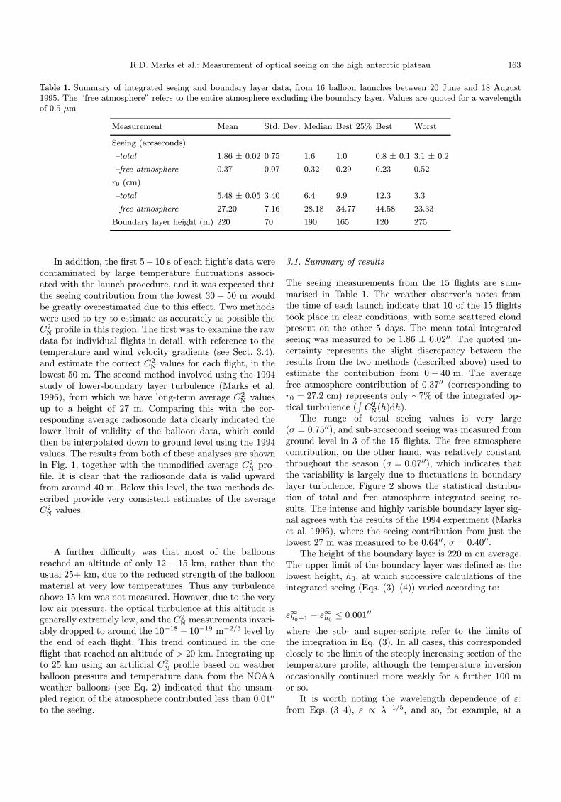
Table 1. Summary of integrated seeing and boundary layer data, from 16 balloon launches between 20 June and 18 August1995. The “free atmosphere” refers to the entire atmosphere excluding the boundary layer. Values are quoted for a wavelengthof 0.5 µm

Measurement Mean Std. Dev. Median Best 25% Best Worst

Seeing (arcseconds)

–total 1.86 ± 0.02 0.75 1.6 1.0 0.8 ± 0.1 3.1 ± 0.2

–free atmosphere 0.37 0.07 0.32 0.29 0.23 0.52

r0 (cm)

–total 5.48 ± 0.05 3.40 6.4 9.9 12.3 3.3

–free atmosphere 27.20 7.16 28.18 34.77 44.58 23.33

Boundary layer height (m) 220 70 190 165 120 275

In addition, the first 5− 10 s of each flight’s data werecontaminated by large temperature fluctuations associ-ated with the launch procedure, and it was expected thatthe seeing contribution from the lowest 30− 50 m wouldbe greatly overestimated due to this effect. Two methodswere used to try to estimate as accurately as possible theC2

N profile in this region. The first was to examine the rawdata for individual flights in detail, with reference to thetemperature and wind velocity gradients (see Sect. 3.4),and estimate the correct C2

N values for each flight, in thelowest 50 m. The second method involved using the 1994study of lower-boundary layer turbulence (Marks et al.1996), from which we have long-term average C2

N valuesup to a height of 27 m. Comparing this with the cor-responding average radiosonde data clearly indicated thelower limit of validity of the balloon data, which couldthen be interpolated down to ground level using the 1994values. The results from both of these analyses are shownin Fig. 1, together with the unmodified average C2

N pro-file. It is clear that the radiosonde data is valid upwardfrom around 40 m. Below this level, the two methods de-scribed provide very consistent estimates of the averageC2

N values.

A further difficulty was that most of the balloonsreached an altitude of only 12 − 15 km, rather than theusual 25+ km, due to the reduced strength of the balloonmaterial at very low temperatures. Thus any turbulenceabove 15 km was not measured. However, due to the verylow air pressure, the optical turbulence at this altitude isgenerally extremely low, and the C2

N measurements invari-ably dropped to around the 10−18 − 10−19 m−2/3 level bythe end of each flight. This trend continued in the oneflight that reached an altitude of > 20 km. Integrating upto 25 km using an artificial C2

N profile based on weatherballoon pressure and temperature data from the NOAAweather balloons (see Eq. 2) indicated that the unsam-pled region of the atmosphere contributed less than 0.01′′

to the seeing.

3.1. Summary of results

The seeing measurements from the 15 flights are sum-marised in Table 1. The weather observer’s notes fromthe time of each launch indicate that 10 of the 15 flightstook place in clear conditions, with some scattered cloudpresent on the other 5 days. The mean total integratedseeing was measured to be 1.86 ± 0.02′′. The quoted un-certainty represents the slight discrepancy between theresults from the two methods (described above) used toestimate the contribution from 0− 40 m. The averagefree atmosphere contribution of 0.37′′ (corresponding tor0 = 27.2 cm) represents only ∼7% of the integrated op-tical turbulence (

∫C2

N(h)dh).The range of total seeing values is very large

(σ = 0.75′′), and sub-arcsecond seeing was measured fromground level in 3 of the 15 flights. The free atmospherecontribution, on the other hand, was relatively constantthroughout the season (σ = 0.07′′), which indicates thatthe variability is largely due to fluctuations in boundarylayer turbulence. Figure 2 shows the statistical distribu-tion of total and free atmosphere integrated seeing re-sults. The intense and highly variable boundary layer sig-nal agrees with the results of the 1994 experiment (Markset al. 1996), where the seeing contribution from just thelowest 27 m was measured to be 0.64′′, σ = 0.40′′.

The height of the boundary layer is 220 m on average.The upper limit of the boundary layer was defined as thelowest height, h0, at which successive calculations of theintegrated seeing (Eqs. (3)–(4)) varied according to:

ε∞h0+1 − ε∞h0≤ 0.001′′

where the sub- and super-scripts refer to the limits ofthe integration in Eq. (3). In all cases, this correspondedclosely to the limit of the steeply increasing section of thetemperature profile, although the temperature inversionoccasionally continued more weakly for a further 100 mor so.

It is worth noting the wavelength dependence of ε:from Eqs. (3–4), ε ∝ λ−1/5, and so, for example, at a


wavelength of 2.4 µm, the corresponding values are 1.36′′

for the full atmosphere and 0.27′′ for the free atmosphere.This particular wavelength is of significance since it is inthe so-called “cosmological window”: a waveband corre-sponding to a natural minimum in airglow emission, andat which the sky brightness due to thermal emission at theSouth Pole is a factor of 10–100 lower than at any otherground-based site (Ashley et al. 1996).

3.2. Comparison with H-DIMM observations

A modified version of a differential image motion monitor,known as an “H- DIMM” (Bally et al. 1996) was alsoin place at the South Pole during 1995. This instrumentconsisted of a 60 cm telescope with a multiple-aperturemask, and is essentially similar in principle to the standardDIMM as described by Sarazin & Roddier (1996).

Seeing measurements were taken by the H-DIMMnear-simultaneously with a microthermal balloon flighton 5 occasions during the season. The results are com-pared in Fig. 3. The correlation between the two exper-iments is reasonably good for three of the flights, whilefor the other two, the microthermal data gives a signif-icantly lower value for the FWHM seeing than does theH-DIMM. These discrepancies are most probably due toserious disturbances in the H-DIMM images caused by in-ternal heaters being inadvertently left on during many ofthe observations, a problem which was not noticed untilafter the completion of the experiment. These distortionswere thought to be largely confined to one particular re-gion of the image data, which was removed during thereduction process. However, it is possible that some effectof this heating was present across the rest of the image,which may have artificially elevated the derived seeing. Asmall residual effect of this nature would be most notice-able at times of relatively low atmospheric seeing, as wasthe case for the two observations in question.

3.3. Individual flight characteristics; relation of boundarylayer seeing to atmospheric parameters

The vertical profile of the optical turbulence at the SouthPole is markedly different from that measured using simi-lar techniques at other sites around the world. Figure 4 isa plot of C2

N vs. altitude for three of the balloon launches,and illustrates the conditions typically observed. Potentialtemperature1 and wind velocity gradients are also in-cluded in the boundary layer profiles (Figs. 4a,c,e). Notethat different scales are used on the C2

N axes for the threeboundary layer plots.

1 Potential temperature is defined as: θ(h) =

T (h)(P (h)1000

)−0.288.

0 1 2 3 4

0

1

2

3

4

0

20

40

60

80

100 %

0.2 0.4 0.6

0

1

2

3

4 %

0

20

40

60

80

100

Fig. 2a and b. Seeing data statistics for the 15 balloon son-des launched in 1995: a) total (from ground level), b) freeatmosphere

The boundary layer turbulence structure is quite com-plex, and contains several strong C2

N peaks, generally oc-curring in layers around 10− 20 m in thickness. The mostintense of these are often concentrated in two regions; oneclose to the surface (up to 50−100 m), and another closerto the top of the inversion layer (∼200 m). This featureis clearly evident in Figs. 4a,c, and was observed in manyof the other flights. It corresponds to a “two-tiered” tem-perature inversion, as indicated by the secondary rise indθ/dz in each of these flights.

The layers of intense optical turbulence, and its overallrapid decrease with altitude, are strongly correlated withsimultaneous sharp fluctuations in dθ/dz and |dU/dz|, ascan be seen clearly in the three flights shown. Figure 5


2900 3000 3100 32000 -0.2

0

0.2

0.4

altitude (m)

4000 6000 80000

altitude (m)

2900 3000 3100 32000 -0.2

0

0.2

0.4

altitude (m)

4000 6000 80000

altitude (m)

2900 3000 3100 32000 -0.2

0

0.2

0.4

altitude (m)

Fig. 4a-f. C2N vs. altitude: a-b) for 23/06/95, c-d) for 21/07/95, e-f) for 18/08/95. The boundary layer plots include potential

temperature gradient, |dθ/dz| (dashed lines) and wind velocity gradient, |dU/dz| (dotted lines). The axes on the right of eachplot show |dθ/dz|, in units of ◦C/m−1. Units for |dU/dz| are not shown; it is approximately equal to 0.5 (RHS axis scale) m s−1,offset by −0.05 for clarity

shows the average profiles of these quantities along withthe C2

N measurements. The mean temperature inversionmagnitude is ∼25◦C. These observations agree with theknown requirements for optical turbulence: the presenceof both a significant temperature gradient and mechanicalturbulence produced by wind shear. In other words, it isthe combination of a strong temperature inversion and awind velocity gradient which produces such a strong seeingcontribution close to the surface, as can be seen clearly inFig. 5.

The occurrence of sub-arcsecond seeing from groundlevel (observed on three occasions) tended to coincidewith a shift in wind direction away from the bearing ofthe usual katabatic flow (between grid N and E) toward

the SE quadrant, with a corresponding increase in surfacelevel temperature and decrease in wind speed. The tem-perature during the best seeing conditions observed (0.8′′)was −42◦C, about 18◦C above average. These influxes ofrelatively warm air from the coast onto the plateau occurvery occasionally throughout the winter. The markedlyimproved seeing that occurs during these events highlightsthe importance of the katabatic wind to the generation ofoptical turbulence in the boundary layer.

Relatively poor seeing (> 2.5′′), tended to occur duringfairly typical wind and temperature conditions. However,the three worst boundary layer seeing measurements co-incided with a very pronounced “double inversion”, as


160 170 180 190 200 2100

1

2

3

4

Fig. 3. Comparison of H-DIMM (triangles) and microthermal(crosses) seeing measurements on the five occasions that thetwo experiments were performed simultaneously, from 23 Juneto 21 July, 1995. The error bars derive from the uncertainty inthe C2

N values from 0− 40 m

described previously, with very intense C2N peaks in the

upper part of the boundary layer.In all but one of the flights, the free atmosphere tur-

bulence was very weak, with the strongest peaks usu-ally around two orders of magnitude weaker than thosemeasured in the boundary layer. There was very littletropopause instability observed in any of the data, withoccasional layers of increased optical turbulence not re-stricted to any particular region of the atmosphere.

The conditions for wind-generated turbulence are oftendefined in terms of the Richardson number:

Ri =g

θ

(dθ/dz)

(dU/dz)2

<1

4· (5)

Equation (5) is usually stated as the criterion for the de-velopment of turbulence. This inequality was calculatedfor all flights, and observed to be consistent with the C2

N

measurements in the lower part of the boundary layer as awhole. However, it did not appear to describe very well theintense individual turbulent layers, which often coincidedwith large positive values of dθ/dz. In the free atmosphere,the occasional layers of relatively large C2

N were often as-sociated with dips in Ri below the critical value of 1/4, asshown in the example of Fig. 6. Any features not coincid-ing with a decrease in Ri generally occurred in thin layerswith a sharp rise in θ of up to 1− 2◦C.

0 200 400 600 800 1000-17

-16

-15

-14

0

0.1

0.20

0.1

0.2

Fig. 5. Average C2N, |dθ/dz|, and |dU/dz| profiles up to a height

of 1 km above the surface. Wind velocity data were obtainedfrom weather balloon launches performed almost simultane-ously with our flights

Most of the free atmosphere seeing was caused bythese turbulent layers. The flights where no sharp peaks inC2

N were observed (6 out of 15, including Figs. 4b,f) gaveεFA = 0.23− 0.26′′. Further analysis of the long-term me-teorological records, with regard to the behaviour of Ri

and dθ/dz, will therefore be useful in determining the fre-quency of the best free atmosphere seeing conditions atthe South Pole.

The C2N measurements are in broad agreement with

acoustic soundings performed at the South Pole since 1975(e.g. Neff 1981), as well as other analyses of the meteoro-logical data (Schwerdtfeger 1984; Gillingham 1993). Whilethe acoustic backscatter measurements of C2

N had a lowervertical resolution than the microthermal balloon sondes,they did illustrate the same features, i.e. a complex tur-bulence structure, often split into two layers, extendingup to an altitude of 200− 300 m, with a sharply definedupper limit, and much weaker activity thereafter.

3.4. Comparison with other sites

In contrast to the conditions observed at the South Pole,while the C2

N profiles measured at mid-latitude sites (e.g.Roddier et al. 1990; Vernin & Munoz-Tunon 1994) often


Table 2. Comparison of seeing conditions at the South Pole and some of the world’s major observatory sites. FA, BL and SLrefer to the free atmosphere, boundary layer and surface layer, respectively

Site Altitude Total seeing FA seeing BL seeing SL seeing/ range BL height Reference[m] [′′] [′′] [′′] [′′, m] [m]

South Pole 2835 1.86 0.37 1.78 0.64, 27 220 this work, Marks et al. 1996

Cerro Paranal, 2500 0.64 (median) – – – – Murtagh & Sarazin 1993Chile 0.73 0.4 0.55 – 2000 Fuchs 1995

La Silla, 2400 0.97 0.31 0.85 0.15, 30 800− 1000 ESO-VLT report 1987Chile 0.87 – – – – Murtagh & Sarazin 1993

Mauna Kea, 4200 0.74 0.46 0.52 – – Roddier et al. 1990Hawaii

La Palma, 2100 0.96 0.40 0.73 0.07, 12 1− 2000 Vernin & Munoz-Tunon 1992, 1994Canary Is.

4000 6000 80000

0

10

20

30

Fig. 6. A comparison of C2N and Ri profiles for 02/07/95. 1/Ri

is plotted to show more clearly the regions of instability: anypeaks above the dashed line satisfy Ri < 1/4. The integratedseeing values calculated for this flight were: εtot. = 0.83′′, εFA =0.41′′

show a significant boundary layer contribution to the over-all seeing, it usually extends to at least 1 − 2 km aboveground level, and is invariably of much lower intensity. Inaddition, upper atmosphere turbulence, arising from jetstreams and temperature fluctuations in the tropopause,is often a major component of the seeing at these sites.

Table 3 summarises seeing measurements from some ofthe world’s leading observatory sites. It can be seen quiteclearly that the optical turbulence at the South Pole isconcentrated much closer to the surface than at any ofthese sites. The free atmosphere contribution is compa-rable to or lower than the best quoted results from the

0 100 200 300 400 5000

0.5

1

1.5

2

Fig. 7. Seeing as a function of height of the telescope abovethe surface. The solid line represents average results from ourlaunches at the South Pole, while the dashed line is a sum-mary of a similar experiment performed at the ESO-VLT siteat Cerro Paranal, northern Chile (Fuchs 1995) in May 1993,averaged over 13 flights

other sites. It is important to note that the value of 0.37′′

is calculated upward from ∼200 m above the surface. Thecontribution from the atmosphere above 2000 m (the av-erage boundary layer height at the mid-latitude sites ofsimilar altitude) at the South Pole is < 0.3′′.

As a more direct comparison, Fig. 7 shows the derivedseeing, averaged over the fifteen flights, as a function ofthe altitude at which a hypothetical telescope is placed.This plot is obtained by increasing the lower altitude limitof the integral in Eq. (3) in 5 m steps. The optical tur-bulence falls sharply up to an altitude of ∼120 m, anddecreases more gradually up to 200 m, beyond which the


Fig. 8. Contour map of surface wind speeds over Antarctica,from Dopita 1993, based on results of Schwerdtfeger 1984

very low remaining seeing contribution decreases smoothlywith altitude.

The results of similar experiments (averaged over thir-teen flights) performed at the ESO-VLT site at CerroParanal, Northern Chile (Fuchs 1995), are included in thesame figure. The two data sets were analysed using thesame method. It is clear that, while South Pole is an infe-rior site (in terms of seeing) from ground level, most of theimage degradation occurs very close to the surface. Theseeing is better than that measured at Paranal above analtitude of only ∼100 m. The free atmosphere contribu-tion, i.e. above ∼250 m, is around 60% of the correspond-ing value calculated from the Paranal data.

4. Discussion

4.1. Other possible sites in Antarctica

The South Pole does not lie on one of the highest points ofthe antarctic plateau, and is therefore not expected to rep-resent the best seeing conditions available in Antarctica.The results obtained here lead us to consider the pos-sibility that the 0.3− 0.4′′ seeing measured above the100− 200 m high boundary layer might extend to groundlevel at other sites on the plateau.

The surface winds at the South Pole are of katabaticorigin, due to the descent of cold air from the higher re-gions of the plateau. The strength and direction of thesewinds over the continent are largely dependent on thelocal topography, as illustrated in Fig. 6 (Dopita 1993;Schwerdtfeger 1984). The strong wind shears observed oc-cur at the boundary between this katabatic flow and theupper atmosphere winds, which are generally geostrophic(Schwerdtfeger 1984). At Dome A (4200 m, 82◦S 80◦E),Dome C (3300 m, 74◦S 123◦E), and Dome F (3810 m,

77◦S 40◦E), the three most significant local “peaks” onthe antarctic plateau, these winds do not exist. Dome A,in particular, being the highest point on the plateau, isat the origin of the katabatic flow. It is likely that, at allof these sites, very little optical turbulence is produced inthe boundary layer since, despite the possible presence ofstrong positive temperature gradients such as those mea-sured at the South Pole, there is little mechanical mix-ing of the different temperature layers. If the free atmo-sphere turbulence at these sites is similar to that at theSouth Pole, we would expect to observe very good seeingfrom surface level: quite possibly the best seeing condi-tions available anywhere on the earth’s surface.

In order to measure the important site characteristicsat these locations, an automated astrophysical observa-tory (AASTO) has been built, which contains several in-struments for measurement of the seeing and the atmo-spheric transmission over a wide range of wavelengths.The AASTO is designed to function independently fora full winter season, and is scheduled to be deployed atDome C in 1999, and at Dome A in 2000.

The construction of a permanent station at Dome Chas begun (the France/Italy Concordia Project), and isexpected to be completed by 2000. This will enable theoperation of a similar range of longer term site-testing ex-periments to those currently being conducted at the SouthPole.

In addition, while there are currently no plans for as-tronomical site-testing at Dome F (also known as DomeFuji), a temporary winter station is currently being oper-ated there by Japanese scientists, whose experiments in-clude meteorological balloon sondes, to be launched dur-ing 1997. Access to these data would provide some veryenlightening comparisons to the measurements made atthe South Pole.

4.2. Other astrophysical parameters

The measured C2N profiles allow calculation of several pa-

rameters necessary to determine the feasibility of imagecorrection techniques (adaptive optics and speckle inter-ferometry) at the site, as well as other quantities such asthe scintillation index. Using the notation:

C(x, η) =

∫xη(h)C2

N(h)dh, C(0) =

∫C2

N(h)dh (6)

these quantities are given by Eqs. (7–11) (Roddier 1981;Roddier et al. 1982). The subscripts AO and SI referto adaptive optics and speckle interferometry respectively.

Isoplanatic patch:

θAO = 0.31r0

(C(h, 5/3)

C(0)

)−3/5

(7)

θSI = 0.36r0

(C(h, 2)

C(0)−

(C(h, 1)

C(0)

)2)−1/2

(8)


Table 3. Summary of the calculated values of the astrophysical parameters defined in Eqs. (7–11), based on the 15 balloonflights. The limit of the boundary layer is taken to be 220 m. Values for Cerro Paranal were obtained using the average C2

N

profiles measured at this site (Fuchs 1995), although no wind data were available. Results for La Palma are from Vernin &Tunon-Munoz (1994)

Site θAO [′′] θSI [′′] τAO [ms] τSI [ms] σ2I

mean best mean best mean best mean best mean best

South Pole–total 3.23 6.50 2.76 5.17 1.58 6.09 17.34 35.04 0.070 0.033–B.L. correction 65.35 – 118.22 – 1.62 – 17.81 – – –

Cerro Paranal 1.45 – 1.88 – – – – – 0.16 –

La Palma 1.30 1.62 2.18 2.66 6.64 9.60 12.88 19.52 – –

Coherence time:

τAO = 0.31r0

(C(U, 5/3)

C(0)

)−3/5

(9)

τSI = 0.36r0

(C(U, 2)

C(0)−

(C(U, 1)

C(0)

)2)−1/2

(10)

Scintillation index:

σ2I = 19.12λ−7/6C(h, 5/6). (11)

4.2.1. Isoplanatic patch, coherence time

The isoplanatic angle, θ, depends on the altitude distribu-tion of the turbulent cells producing the seeing, accordingto Eqs. (7–8). This angle represents the maximum angu-lar distance between the source of interest and a referencestar for which the wavefront distortions are coherent andmay, in principle, be fully corrected. The maximum in-tegration time, τ , for which a given correction remainsaccurate is limited by temporal isoplanatism, due to themovement of turbulent cells across the field of view atthe wind velocity, according to Eqs. (9–10). The valuesof these quantities, calculated from the measured C2

N pro-files are shown in Table 3, along with corresponding val-ues from La Palma and Cerro Paranal. The results at theSouth Pole are somewhat better than at the other sites,especially during the best observing conditions. The im-provement is minor, however, especially in the values ofθAO/SI, and does not greatly relieve the problem that theprobability of finding a suitable reference source withinthis area of the sky is extremely low (∼10−3 at visual mag-nitude mv = 16). The relatively large difference betweenτSI and τAO is due to the different C2

N and U profiles,compared with other sites, as discussed in Sect. 3.4.

In practice, varying degrees of partial correction maybe sought, and the performance of such systems has beenanalysed in detail (e.g. Cowie & Songaila 1988; Wilsonet al. 1996). Evidently, the maximum image “reconstruc-tion angle” (the term coined by Cowie & Songaila) de-pends on the degree of correction required. A trade-off

must be made between the quality of the corrected imageand access to enough suitable reference sources to obtainadequate sky coverage.

As discussed previously, the large majority of the op-tical turbulence at the South Pole occurs in the lowest∼200 m. Thus, and due to the strong height dependence ofθAO/SI shown in Eqs. (7–8), we may expect that an imagecorrection system that removed the boundary layer com-ponent of the seeing, leaving the remainder uncorrected,would be effective over a substantially greater area of thesky than such a system operating at the best mid-latitudesites.

In a simple approximation, angles for partial imagecorrection were calculated by varying the upper limits,hu, of the integrals in Eqs. (7–8). The residual seeing, εr,related to each of these angles, may be found by settinghu = h0 in Eq. (3), and using the values calculated inSect. 3.4 (Fig. 7). As expected, the reconstruction angleincreases rapidly for corrections limited to the boundarylayer seeing (i.e. h ' 200 m, εr ' 0.3′′ on average), asshown in Table 3 (θSI = 1′58′′, θAO = 1′6′′), and Fig. 9. Asystem operating at εr = 0.3′′ at Cerro Paranal wouldrequire that hu be much higher (see Fig. 7), resultingin substantially smaller reconstruction angles (θSI = 13′′,θAO = 10′′). Thus, the difference between the sites at thesame level of partial image correction is very large.

The improvement in terms of sky coverage associatedwith the increased partial correction angles can be foundby determining the probability of finding an appropriateguide star of magnitude mv within an angle θ, at Galacticlatitude b (Olivier et al. 1993):

Psky = 1− exp[−πθ2Σ(mv, b)

](12)

where Σ(mv, b) is the number density of stars of a givenmv and b. Values of Σ(mv, b) are tabulated in various as-tronomical data books (e.g. Allen 1973).

From Fig. 9 and Eq. (12), we have a relationship be-tween Psky and the uncorrected component of the see-ing. Figures 10a,b shows this relationship for various val-ues of mv averaged across all galactic latitudes, for bothspeckle interferometry and adaptive optics. Corresponding


0 0.2 0.4 0.6 0.80

20

40

60

80

100

(A.O.)

0 0.2 0.4 0.6 0.80

20

40

60

80

100

(S.I.)

Fig. 10a and b. Percentage sky coverage as a function of the residual seeing, for a) adaptive optics and b) speckle interferometry,in the visual magnitude range mv = 14 − 16. Solid lines show the results for the South Pole; dashed lines for Cerro Paranal.Calculations are averaged over all galactic latitudes

0 0.1 0.2 0.3 0.40

50

100

150

Fig. 9. θAO/SI, as a function of the residual seeing εr. Solid linesare derived from the average C2

N profiles at the South Pole, andthe dashed lines from the Cerro Paranal data. The curves areobtained by varying the upper and lower limits of Eqs. (7)–(8) and Eq. (3), respectively. The value of θ for ε = 0 is theisoplanatic angle

calculations based on the available data from CerroParanal are included for comparison.

Figure 10 shows that the sky coverage is up to around75% for image quality εr = 0.3′′, using reference sourcesin the range mv = 16 to mv = 14. This value decreasessomewhat at the bright end, in the adaptive optics case

(Fig. 10a). The percentage of sky covered at Cerro Paranalover this range of εr and mv is around 1 − 2%. 75% skycoverage would be possible at this site only with imagesin the range εr = 0.4− 0.5′′.

Note that these values are calculated for an “average”number density of stars at each magnitude; the higherdensity near the galactic equator improves the resolutionby ∼0.05′′ for a given value of Psky. A further improve-ment of approximately the same magnitude should alsobe obtained in the infrared, bringing the residual seeingdown to the range εr ∼ 0.1− 0.2′′.

As noted above, these results assume that partial cor-rections may be performed based directly on the altitudedistribution of the turbulent layers. This is not possiblein practice, but, rather, any method of partial correctionmust take into account the power spectrum of the tur-bulence. However, the comparison between the two sitescertainly remains valid, and the results are a good quali-tative indication of the attainable image resolution at thesite.

Some of the practical methods that have been devel-oped to increase the workable angle of adaptive optics sys-tems indicate that the achievable image quality may besignificantly better than the values stated here. Cowie &Songaila (1988) were able to obtain 0.1− 0.2′′ images atMauna Kea over an angle of up to ∼30′′ (a factor of fivegreater than the isoplanatic angle at this site) by relaxingthe requirement of full isoplanicity at high frequencies.

Another method that has been investigated is the“multiconjugate” approach (e.g. Tallon et al. 1992), inwhich a number of deformable mirrors are used, eachplaced conjugate with a turbulent layer. Theoretical


calculations have been performed by Wilson & Jenkins(1996), to determine the relative performance of imagecorrection systems using pupil and turbulence conjuga-tion. It was found that the sky coverage was greater usingturbulence conjugation, compared with pupil conjugation,by a factor of 2−3 (at the same level of image correction).

Turbulence conjugation is a particularly powerful tech-nique in situations where the bulk of the image degrada-tion is concentrated in a small number of turbulent lay-ers, which is clearly seen to be the case at the South Pole(Figs. 4a–f). Since most of the boundary layer turbulenceis confined to ∼ 1 − 3 intense turbulent layers, with per-haps 2− 3 weaker layers throughout the free atmosphere,it can be envisaged that such a system operating at thissite would be capable of very high resolution imagery overa large proportion of the sky.

4.2.2. Scintillation index

The scintillation index, σ2I (Eq. (11)), is a measure of the

amplitude fluctuations in the received signal from an as-tronomical source, caused by atmospheric turbulence. It isan important limiting factor in observations that measuresmall variations in the flux of a source, including obser-vations of variable stars, and asteroseismology. The h5/6

dependence of σ2I indicates that this quantity, too, should

have a lower value at the South Pole than at any othersite.

The results for λ = 0.5 µm, summarised in Table 3 andFig. 11, show that the average value of σ2

I is about 40% ofthe corresponding value calculated from the Cerro Paranaldata (which, again, represents close to the best conditionsmeasured at a mid-latitude site). These results, togetherwith the long continuous observations possible during thepolar night, indicate that the antarctic plateau is an idealsite for the types of observations mentioned above.

5. Conclusion

The atmospheric seeing at the South Pole has been mea-sured during a campaign of 15 balloon launches fromJune–August 1995. The vertical C2

N profiles indicate thepresence of an highly turbulent boundary layer up to analtitude of 100−250 m, with a very stable free atmosphere.

The boundary layer turbulence is closely associatedwith the katabatic wind and surface temperature inver-sion (Fig. 5). This suggests that the seeing at other siteshigher on the plateau, where the katabatic wind is absent,is likely to be substantially lower than the average 1.86′′

(1.36′′ at 2.4 µm) from surface level at the Pole, and maywell approach the 0.37′′ (0.27′′ at 2.4 µm) free atmospherecontribution. This would be significantly better than anyother site studied to date, and, combined with the ex-cellent atmospheric transmission at infrared wavelengths,

0.02 0.04 0.06 0.08 0.1 0.12

0

1

2

3

4

Fig. 11. Distribution of the value of σ2I calculated for each of

the fifteen balloon flights. The highest measured value, σ2I =

0.118, is statistically more than 3σ above the mean, and theC2

N data from this flight were omitted when calculating theaverage value shown in Table 3

the low scintillation index, and the possibility of perform-ing long continuous observations, the potential scientificvalue of an appropriate observatory on the high antarcticplateau is undeniable. It is, of course, necessary to quantifythe atmospheric seeing and transmission characteristics ofsites such as Domes A and C, and such measurements areplanned for the near future.

The vertical C2N profile at the South Pole is favourable

for image restoration using an adaptive optics system thatcorrects for the effects of the boundary layer turbulence.At optical wavelengths, image resolution of <∼0.2′′ FWHMshould be attainable over an angle of 2′ or more, whichwould provide excellent sky coverage even for reasonablybright reference sources. If this level of performance isfound to be practically achievable, it may be that theSouth Pole itself would be a suitable observatory site,given the support infrastructure already in place at thislocation.

Acknowledgements. We wish to thank Al Harper, Bob Pernicand Bob Loewenstein from CARA (the University of Chicago),and John Storey, Michael Ashley and Michael Burton from theUniversity of New South Wales, for their assistance. This re-search was supported in part by the U.S.A. National ScienceFoundation under a cooperative agreement with the Center forAstrophysical Research in Antarctica (CARA), grant numberNSF OPP 89-20223. CARA is a National Science FoundationScience and Technology Center. Support from the AustralianDepartment of Industry Science and Technology’s BilateralProgram is gratefully acknowledged. Funding for all instru-mentation was provided by l’Institut National des Sciencesde l’Univers, France. We make special mention of the late


Jean-Francois Manigault for his part in the successful com-pletion of this research.

References

ESO-VLT working group on site evaluation, 1987, VLT reportNo. 55, M. Sarazin (ed.)

Allen C.W., 1973, Astrophysical Quantities. Athlone PressAshley M.C.B., Burton M.G., Lloyd J.P., Storey J.W.V., 1995,

SPIE 2552, 33Ashley M.C.B., Burton M.G., Storey Lloyd J.P., et al., 1996,

PASP 108, 721Bally J., Theil D., Billawala Y., 1996, Proc. Astron. Soc. Aust.

13, 22Burton M.G., Aitken D.K., Allen D.A., et al., 1994, Proc.

Astron. Soc. Aust. 11, 127Burton M.G., 1996, Pub. Astron. Soc. Aust. 13, 2Cowie L.L., Songaila A., 1988, J. Opt. Soc. Am. 5, 1015Dierickx P., 1992, J. Mod. Opt. 39, 569Dopita M.A., 1993, IABO: The International Antarctic Balloon

Observatory (draft copy)Forbes F.F., 1989, SPIE 1114, 28Fried D.L., 1966, J. Opt. Soc. Am. 56, 1372Fuchs A., 1995, Contribution a l’etude de l’apparition de la

turbulence optique dans les couches minces. Concept duSCIDAR generalise (Ph. D. Thesis), Universite de Nice-Sophia Antipolis, France

Gillingham P.R., 1993, ANARE Res. Notes 88, 290,Australian Institute of Physics 10th Congress, Universityof Melbourne, February 1992 (publications of the AntarcticDivision)

Marks R.D., Vernin J., Azouit M., et al., 1996, A&AS 118, 385Murtagh F., Sarazin M., 1993, PASP 105, 932

Neff W.D., 1981, An Observational and Numerical Study of theAtmospheric Boundary Layer Overlying the East AntarcticIce Sheet (Ph. D. thesis), Wave Propagation Laboratory,Boulder Colorado, U.S.A.

Nguyen H.T., Rauscher B.J., Severson S.A., et al., 1996, PASP108, 718

Obukhov A.M., 1949, Izv. Akad. Nauk SSSR, Ser Geograf.Geofis. 13, 58

Olivier S.S., Max C.E., Gavel D.T., Brase J.M., 1993, ApJ 407,428

Parenti R.R., 1992, Lin. Lab. J. 5, 93Roddier F., 1981, Prog. Opt. 19, 281Roddier F., Gilli J.M., Lund G., 1982, J. Opt. Paris 13, 263Roddier F., Cowie L., Graves J.E., et al., 1990, SPIE 1236, 485Sarazin M., Roddier F., 1990, A&A 227, 294Schwerdtfeger W. (ed.), 1984, Weather and Climate of the

Antarctic. Elsevier Science Pub. Co. NYStorey J.W.V., Ashley M.C.B., Burton M.G., 1995, Publ.

Astron. Soc. Aust. 13, 35Tallon M., Foy R., Vernin J., 1992, Laser guide star adaptive

optics workshop, Fugate R.Q. (ed.), Albuquerque (10–12March 1992)

Tatarski V.I., 1961, Wave Propagation in a Turbulent Medium.McGraw-Hill, New York

Vernin J., 1994, Recherche de site pour l’astronomie enAntarctique, Colloque Acad. Sci. Paris, 16-18 Dec. 1992,92-96

Vernin J., Marks R., Ashley M.C.B., et al., 1994, OpticalTurbulence at the South Pole: First Measurements andFuture Plans, XXIIIrd SCAR Meeting, Rome, Aug. 29-Sep.1

Vernin J., Munon-Tunoz C., 1992, A&A 257, 811Vernin J., Munon-Tunoz C., 1994, A&A 284, 311Wilson R.W., Jenkins C.R., 1996, MNRAS 268, 39

measurement of optical seeing on the high antarctic … r.d. marks et al.: measurement of optical...

Documents