alamos - digital library/67531/metadc688500/m2/1/high... · transims predicts trips for individual...

I

LA-UR- 98-3162

Title:

Aut hor(s):

Submitted to:

Los Alamos N A T I O N A L L A B O R A T O R Y

A COMPARISON OF EMISSIONS ESTIMATED IN THE TRANSIMS APPROACH WITH THOSE ESTIMATED FROM CONTINUOUS SPEEDS AND ACCELERATIONS

M. D. Williams G. R. Thayer L. Smith

Transportation Research Board Washington, DC January 1999 E

Los Alarms National Laboratory, an affinnative actidequal opportunity employer, is operated by the University of California for the

O o v m retains a nonexclusive, myalty-free license to publish or reproduce the published form of this contribution, or to allow athers to do so, for U.S. Government p w p ~ ~ e s . Los Alamos National Laboratory requests that the publisher identify this article as vmk petformed underthe auspices of the U.S. Department of Energy. The Los Alamos National Laboratory strongly supports academic frwcbm and a resBBrchB('s right to publish; as an institution, however, the Laboratory does not endorse the viewpoint of a publication or guarantee its technical correctness.

US. Department of E W rtnder contract W-7405-ENGa. By acceptance of thls article, the publisher recognize that the U.S.

Form 836 (l(Y96)

This rrpon was prepared as an account of work s p o d by an agency of the United States Government Neither the United Statu Govanmcnt nor my agcacy thereof, nor any of thcir employas makes any wuraaty, cxprrrt or implied, or assumes my leg@ liability or rrspowiiiity for the acamq, compieteacss, or use- fulness of any infomation, apparatus, pmdwt, or pmcas disdod, or rrprrscnu that its w would not infringe privatciy owued rights. Rcferrncc hadn to any sp- d l C commercial ptodun, pmcsr, ot semice by trade nanm tldcmck iaaaufac- turn, or otherwise docs not necessarily consticute or imp& iu odonemenr, rrcom- mendation. or favoring by tbe United States Govanment or ray agency thereof. Tfie views and opinions of authors qmsscd herein do not WQgOrily state or reflect thore of tbc United States Govanmast or any rseny thereof.

DISCLAIMER

Portions of this document may be illegible in electronic image products. Images are produced from the best available original document.

I- J

' 0 . . Williams, Thayer, and Smith

A COMPARISON OF EMISSIONS ESTIMATED IN THE TRAN- SIMS APPROACH WITH THOSE ESTIMATED FROM CONTIN- UOUS SPEEDS AND ACCELERATIONS

MichaelD. -Williams, Gary Thayer, and LaRon Smith

Technology and Safety Assessment Division, Los Alamos National Laboratory, Los Alamos, NM

87545

ABSTRACT

TRANSIMS is a simulation system for the analysis of transportation options in metropolitan areas.

It's major functional components are: (1) a population disaggregation module, (2) a travel planning

module, (3) a regional microsimulation module, and (4) an environmental module. In addition to

the major functional components, it includes a strong underpining of simulation science and an an-

alyst's tool box. The purpose of the environmental module is to translate traveler behavior into con-

sequent air quality. The environmental module uses information from the TRANSIMS planner and

the microsimulation and it supports the analyst's toolbox.

Transportation systems play a significant role in urban air quality, energy consumption and carbon-

dioxide emissions. Recently, it has been found that current systems for estimating emissions of pol-

lutants from transportation devices lead to significant inaccuracies. Most of the existing emission

modules use very aggregate representations of traveler behavior and attempt to estimate emissions

on typical driving cycles. However, recent data suggests that typical driving cycles produce rela-

tively low emissions with most emissions coming from off-cycle driving, cold-starts, malfunction-

ing vehicles, and evaporative emissions. Furthermore, some portions of the off-cycle driving such

* 9.

1

Williams, Thayer, and Smith 2

as climbing steep grades are apt to be correlated with major meteorological features such as downs-

lope winds. These linkages are important, but they are not systematically treated in the current

modeling systems. The TRANSIMS system holds the promise of a more complete description of

the role of heterogeneity in transportation in emission estimation.

The TRANSIMS micro-simulation produces second by second vehicle positions defined by 7.5

meter cell locations. An approach has been used to convert average cell populations and average

transitions between cells into fine-grained distributions of speeds and accelerations. This paper de-

scribes the approach and compares the emissions that result from: (1) actual measured trajectories,

and (2) the transims approach applied to cell positions extracted from the actual trajectories. Seven

different levels of congestion of freeways are examined and three different groupings of arterials

were analyzed.

OVERVIEW

Transportation activities contribute to excessive ozone, carbon-monoxide, and respirable particu-

late matter concentrations in urban areas. The air quality community has developed a number of

tools to address these problems. Emissions typically have been estimated by assuming that people

use driving patterns similar to those over which the emissions of vehicles have been tested. With

these formulations, estimates of vehicle miles traveled and average speeds can be used to estimate

emissions. This basic formulation has been supplemented by corrections for cold starts, evapora-

tion from fuel tanks, and super-emitting vehicles. Recently, it has been found that current systems

for estimating emissions of pollutants from transportation devices lead to significant inaccuracies

'.. One possible contributor to the inaccuracies results from deviations from the standard driving

”?. c .

I Williams, Thayer, and Smith

~

3

cycles that produce dramatically increased emissions ’. Of particular concern is the effect of slopes

I because slopes also influence the local meteorology. When these inaccuracies are coupled to air

quality models and limited meteorological data, it is difficult to tell whether the most appropriate

path is being taken to achieve air quality goals ’.

The TRansportation ANalysis and SIMulation System (TRANSIMS) is being developed to ad-

dress this problem as well as many other transportation analysis challenges. TRANSIMS is one

part of the multi-track Travel Model Improvement Program sponsored by the U. S. Department of

Transportation, the Environmental Protection Agency, and Department of Energy. Los Alamos

National Laboratory is leading this major effort to develop new, integrated transportation and air

quality forecasting procedures necessary to satisfy the Intermodal Surface Transportation Efficien-

cy Act and the Clean Air Act and its amendments.

TRANSIMS is a set of integrated analytical and simulation models and supporting data bases. The

TRANSIMS methods deal with individual behavioral units and proceed through several steps to

estimate travel. TRANSIMS predicts trips for individual households, residents and vehicles rather

than for zonal aggregations of households. TRANSlMS also predicts the movement of individual

freight loads. A regional microsimulation executes the generated trips on the transportation net-

work, modeling the individual vehicle interactions and predicting the transportation system perfor-

mance.

The purpose of the TRANSIMS environmental module is to translate traveler behavior into conse-

quent air quality, energy consumption, and carbon dioxide emissions. There are four major tasks


required to translate traveler behavior into environmental consequences: ( 1) estimate the emis-

sions, (2) describe the atmospheric conditions into which the contaminants are emitted, (3) de-

scribe the local transport and dispersion, and (4) describe the chemical reactions that occur during

transport and dispersion of the contaminants.

The choice of components in the TFUNSIMS approach is driven by the goal of representing those

details that may influence the answer of the question being asked. In the context of travel the focus

is on the individual traveler. In a same vein, the atmospheric model is chosen to be one that uses a

relatively complete description of the physics of atmospheric circulation and includes an explicit

treatment of the role of turbulence. The dispersion model is chosen to be a Monte-Carlo kernel

model that can treat the effects of wind-shear, terrain flows and terrain-induced turbulence. The

photochemical model is an airshed model.

METHODOLOGY

The TRANSIMS architecture includes four major elements: (1) a household and commercial ac-

tivity disaggregation module, (2) an intermodal route planner, (3) a travel microsimulation module,

and (4) an environmental module. The disaggregation module uses census and survey data to con-

struct a regional synthetic population. In the future, it will also estimate travel related activities for

each member of the synthetic population. Currently, travel activities are inferred from origin and

destination matrices developed by regional planning authorities. The intermodal planner produces

planned travel link by link and mode by mode on the travel network. The microsimulation module

executes the planned travel over the urban area. The TRANSIMS environmental module is com-

posed of a system of environmental modules that can describe both the average conditions and the

fluctuations about the averages.

Williams, Thayer, and Smith

ist of surface characteristics, large-scale meteorology, terrain, trav-

eler behavior, and vehicle characteristics. Terrain and surface characteristics for current conditions

are available for US cities. For future applications, estimates will have to be made of the changes

expected from the current conditions. The required large-scale meteorology is available through

airport radio balloon soundings or through meteorological analyses done by the National Meteo-

rological Center.

. -

5

Household and Commercial Activity Disaggregation Module

The disaggregation module includes two components: ( 1) a synthetic population submodule and

(2) an activity demand submodule. The synthetic population is developed from the Census Stan-

dard Tape File 3 (STF-3) and the Public Use Microdata Sample (PUMS). The PUMS has all the

desired attributes of the population but it represents a sample from a much larger population than

desired while the STF-3 represents a much smaller population, but it doesn't provide all the infor- 1

mation of interest. A statistical technique called iterative proportional fitting is used to estimate the

desired data at the census tract or block group level based on the PUMS correlations. The actual

synthetic population is randomly drawn from the multi-way tables produced by iterative propor-

tional fitting.

The activity demand module is not yet developed. In the interim, a module that uses the metro-

politan planning organization's estimated origin and destination tables to produce synthetic activ-

ities is being used.

. ... . . .


The Intermodal Route Planner

6

The planner generates routes for each load from the activity-based travel demand. A load is a trav-

eler or a commodity. A trip plan is a sequence of modes, routes and planned departure and arrival

times at the origin, destination(s), and mode changing facilities to move the load to its activity lo-

cations. We assume that travel demand derives from a load's desire or need to perform activities.

The household and commercial activity disaggregration module provides the planner with disag-

gregated activity demand and travel behavior. The planner assigns activities, modes, and routes to

individual loads in the form of trip plans. The individual trip plans are input to the travel microsim-

ulation for its analysis.

Trip plan selection is related directly to a loads desire to satisfy individual (or in the case of freight,

corporate) goals. Goals measure a trip plan's acceptability and depend on the load's socioeconomic

attributes and trip purpose. Typical goals include cost, time, and distance minimization, and safety

and security maximization. The load's objective is to minimize the deviations from these goals.

The travel demand problem is formulated as a mathematical program based on a multi-goal objec-

tive function. The Planner's solution method has four phases: (1) trip generation, (2) goal measure-

ment, (3) preference adjustment, and (4) trip plan superposition. In the first three phases, the

individual's travel behavior preferences such as departure time or origin-destination directness, are

adjusted iteratively to satisfy the travel goals. After every load has a feasible trip plan, the fourth

phase superimposes all trip plans on one another in space and time. The network characteristics are

then updated based upon the projected interaction of all trips and steps (1) through (4) are repeated.


Travel Microsimulation

7

The Travel Microsimulation module mimics the movement and interactions of travelers through-

out a metropolitan region’s transportation system. The approach is to use a cellular automata (CA)

microsimulation. CA traffic models divide the transportation network into a finite number of cells.

In the current form each cell’s length is the average distance between vehicles when traffic is at a

complete standstill. A cell may be empty or contain a single vehicle. If it contains a vehicle, the

vehicle has an integer velocity between zero and maximum velocity, Vmax=5. The integer velocity

represents the number of cells that vehicle moves the next step. The step size is exactly one second,

in which case Vmax corresponds to 135 km/hour, or about 84 mph. This step size abets fast com-

putation because the updated vehicle position is computed by integer arithmetic and without mul-

tiplication of velocity and time step.

Updating the vehicle’s next velocity and position is quite simple. First, we define the number of

unoccupied cells ahead of the vehicle as its “gap”. Then, we update the velocity by accelerating to

the maximum velocity without running into the vehicle ahead:

V(t+ l)=min[V(t)+l ,Vmax,gap].

But, with probability P, we reduce this tentative velocity by one (without going backwards):

V(t+ l)=max[V(t+ 1)- 1,0].

-.- -. f


Finally, we update the vehicle's position:

X(t+ l)=X(t)+V(t+l).

This rule set is called the Nagel-Schreckenberg model. The random velocity reduction process cap-

tures driver behavior such as free-speed driving fluctuations, non-deterministic accelerations, and

overreactions when braking. The simple one-lane model has been extended to cover lane changing,

passing, merging, and turning behaviors.

The simple model produces dynamics observable in everyday freeway traffic. First, we can display

an individual vehicle's movement in space and time as shown in Figure 1. Vehicles moving at con-

stant velocity leave straight-line tracks slanting downward to the right. A stopped vehicle moves

in time, but not in space, creating a vertical line. The figure shows the spontaneous formation of

well-known traffic shock waves that propagate backward in space.

Emissions Modules

An essential component for TRANSIMS is an emissions model that can give emissions specific to

the type of driving being done. In this paper we report results-based on a model developed by in-

vestigators at the University of Michigan4. The emissions describe a composite vehicle and are

based on FTP-revision studies by the US EPA'. Currently, we are only estimating emissions from

normally operating vehicles with hot catalyts and warm engines. Malfunctioning vehicles, cold

starts, and more vehicle types will be addressed when we replace the University of Michigan model

with one developed by University of California at Riverside and University of Michigan investi-

gators who are working on a contract for the National Cooperative HIghway Research Program.

-.- -. f


Williams, Tbayer, and Smith

Evaporative emissions are not discussed in this paper.

9

I , * -

The primary output of the transportation micro-simulation module will be summarized cellular-au-

tomata (CA) data. The CA describes the vehicle position in units of cells, velocity in units of cells

per second and the acceleration in units of cells per second per second. A typical cell size is 7.5

meters so that the resulting motion, in 16 mph increments, is too coarse to be used directly as input

to the emissions module. We are developing an approach to produce realistic, smooth vehicle tra-

._ - .

jectories that can be used in the emissions module.

The challenge is to provide an adequate representation of actual speeds and accelerations. Since

those few vehicles that have sufficient acceleration to produce enriched operation will contribute

disproportionally to the total emissions it is important to represent the tails of the acceleration dis-

tribution. In order to address this question we examined the three cities data and looked at the fre-

quency distribution of accelerations. Figure 2 reports such a distribution for vehicles with speeds

greater than 1 CA cell per second. If we look at the vehicles with higher accelerations we see that

a good fit to the curve is obtained with an exponential in the velocity-acceleration product. With

this information as a guide we have chosen to consider all accelerations or decelerations in three

groups: (1) hard accelerations to represent the ten percent most aggressive accelerations, (2) insig-

nificant accelerations, and (3) hard decelerations.Within the hard acceleration or hard deceleration

groups we will pick several points on the conditional acceleration curves to describe different lev-

els of aggressiveness.

With this approach we need to estimate the speed distribution and the probability of a hard accel-


eration, an insignificant acceleration, and a hard deceleration The most important task is to deter-

mine the fraction of the vehicles undergoing hard acceleration because the emissions are more

sensitive to hard accelerations than they are to decelerations.

The speed distribution can be estimated by fitting a continuous distribution to the spatial and speed

CA populations. We use a constant (fij) plus a term (hi$ proportional to velocity within the cell and

require that the distribution is continuous between velocity cells for a given spatial cell.

In this notation the i index refers to the speed bin and the j index refers to the spatial cell. In this

formulation the speed is written as:

v = (i- 1)A+6v,

with A as the CA speed bin size, 7.5 meters per second and 6 v the speed relative to the lower limit

of the speed bin. The position is given by:

x = xi + 6 x .

If the speed remains constant over the next second, the new position is:

which allows us to calculate the new CA speed bin as:

x, - x j A

6 x + ( i - 1 )A + 6v - 6xn A = 1 + k = 1 +


This expression allows us to develop inequalities that describe what combinations of 6x and 6 v

will permit the vehicle to remain in the same speed bin (k=j) or jump to the next higher speed bin.

We can then calculate the total spatial and speed cell populations as:

Note that with speeds spanning five cells we will CA populations in six speed bins. We use the

continuity requirements plus the conditional that the vehicle density goes to zero at the top of the

last cell along with the CA population relationships to calculate the velocity distribution parame-

ters fij and hij.

The next question is what are the probabilities of a hard acceleration in a given cell? Accelerations

arise in two ways: (1) there is ensemble acceleration as for example, vehicles leave a stop or accel-

erate up an on-ramp and (2) there is individual acceleration as vehicles escape from spontaneous

traffic jams. In the latter case, if we look at cell populations averaged over times long compared to

the jam formation and dissolution, the cells will display a speed distribution that reflects vehicles

slowing down for jams and speeding up on the downstream side of the jams. A logical parameter

to capture this type of accelerations is the standard deviation of the speeds. In the case of the bulk

accelerations, we need a parameter that reflects changes in the product of the vehicle density (in

both space and velocity space) and the product of acceleration and speed. Since we can express

acceleration as a = -v , we need a parameter of the form v - or to within a constant- . Spe- av 2av av3 ax ax ax


cifically, we use the parameter:

12

a JV'(f + h6v)dv sp = -[ ax J(f + hSv)dv ).

With the parameters chosen, we next have to find the appropriate constants. The approach is to as-

sume that the probability of a hard acceleration is proportional to difference between the chosen

parameter and a threshold until a saturation value is reached after which the probability is constant.

In order to find the appropriate constants w e began with actual vehicle trajectories from a database

developed by the California Air Resource Board'. We overlaid a grid on the vehicle's trajectory

and deduced equivalent CA positions and velocities. For each actual trajectory, we constructed 400

trajectories slightly offset in time and space to more accurately represent the cell positions expect-

ed in real traffic. When we accumulated positions, we weighted the number by the inverse of the

total number of all trajectories with the result that the emissions represent those of a single average

vehicle.

The trajectories were grouped into 10 sets; three sets of arterials, slow, medium, and fast, and 7

freeway sets ordered by increasing congestion. The most uncongested freeway set had average

speeds of about 60 mph while the most congested set had average speeds of about 10 mph. In each

case we used only the first 30 seconds of the driving. From the synthetic CA data we collected the

fraction of the vehicles in each CA speed bin in each CA cell. We lumped the populations from

four spatially adjacent cells for computational efficiency. We fit the cell populations with our con-

tinuous distributions and estimated the standard deviations of the velocities and estimated sp for

each spatial cell. We then chose thresholds, slopes, and saturation values for both the standard de-


viations and sp. With the resulting hard acceleration probabilities we obtained the acceleration dis-

tribution for each spatial and speed cell and combined that with the speed distribution to provide

input to the emission model. We also took the speeds and accelerations from the actual trajectories

and compared the resulting emissions to those produced from the synthetic CA data. We used the

resulting information to improve our estimates of the fitting constants.

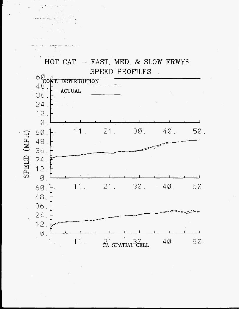
The averages of speeds, CO emissions, NOX emissions, hydrocarbon emissions, and fuel con-

sumption were compared to those from the original trajectories. Figure 3 reports such a comparison

for speeds for the fastest freeway (top), a mid-range freeway (middle, set 3), and a very slow free-

way (bottom, set 6). The speeds show large differences among the tree sets and the constructed

continuous distribution is very close to the actual distribution. The apparent increase of speeds with

distance in the slower sets results from slower vehicles disappearing from the set after 30 seconds

without reaching the more distant CA cells. Figure 4 reports the comparison for NOX emissions

for the aforementioned freeway sets. Once again the constructed distribution is quite close to the

actual distribution. However, there is very little difference in NOX emissions among the three sets

except in the downstream portions of the two lower plots where many of the vehicles have disap-

peared. Figure 5 shows a similar plot for hydrocarbon emissions. In this case there are some dif-

ferences relating to the starts of the trajectories associated with the artificialities of the trajectories.

Figure 6 reports a similar plot for CO emissions. In this plot, the slowest set has somewhat lower

emissions as opposed to the other two.

Figure 7 reports the speed comparisons for the fast (top), medium (middle), and slow (bottom) ar-

terials. Once again, the fits are quite good. In Figure 8 we have the plots for NOX emissions, that

i,


show a large hump associated with some of the vehicles starting out from a red light while others

passed through on green. There is not much difference between the plots, except that the high emis-

sion hump is more extended for the higher speed arterial. Generally the constructed model does

very well, although there some spurious humps that might suggest a need for better smoothing. Fig-

ure 9 reports hydrocarbon emissions and Figure 10 reports CO emissions.

Overall the model shows good agreement with the emissions estimated for the actual trajectories.

Furthermore, there is relatively little difference in emissions between the various conditions. The

most important emissions changes occur when there are vehicles accelerating out from a stop. The

acceleration of vehicles up to speed after spontaneous traffic jams also plays a significant role.

Currently, the modal emission model takes the form of an array that translates speeds and acceler-

ations into emissions of composite vehicles. In the future, it may be useful to consider the history

effects on emissions. In such an instance we can use our estimated acceleration probabilities to con-

struct trcjectories for different levels of aggressiveness and process the trajectories with an emis-

sion module that takes into account the history effects on emissions.

SUMMARY

The TRANSIMS environmental module uses inputs from the TRANSIMS planner and traffic mi-

crosimulation. An examination of the consequences of coarse-graining actual trajectories into CA

bins shows that a good representation of actual emissions can be obtained. The representation was

good even though the data set includes circumstances under which enrichment can occur. Enrich-

ment conditions pose a challenge, because the emissions can be very sensitive to magnitude and


frequency of accelerations. Rarely do we have data that permits an estimation of the high-end tail

of the acceleration distribution.

The major elements responsible for emissions are organized accelerations such as those that occur

when leaving a stop and incoherent accelerations as individual vehicles resume speed after leaving

a spontaneous traffic jam. Speed alone does not appear to be a major factor in NOX emissions,

when emissions are compared on a per vehicle entering the link and per unit space basis.

ACKNOWLEDGMENTS

This work was supported by the US Department of Transportation and the US Environmental Pro-

tection Agency. The filter program uses a least squares solver developed by P. Spellucci (spelluc-

[email protected]). Myron Stein was of great help in the code development.

REFERENCES

1. Oliver, W.R., R.J.Dickson, and L. Bruckman, “Development of the SCAQS High-Resolution

Emissions Inventory: Assessment of Inventory Uncertainties,” in Proceedings of an International

Specialty Conference, Southern California Air Quality Study, Data Analysis, VIP-26 published by

the Air & Waste Management Association 1993, Pittsburgh, Pennsylvania,. pp 62-73.

2. Kelly, Nelson A. and Peter J. Groblicki, “Real-World Emissions from a Modern Production Ve-

hicle Driven in Los Angeles,” J. Air Waste Management Assoc.1993,43, pp 1351-1357.

3. National Research Council, “Rethinking the Ozone Problem in Urban and Regional Air Pollu-


tion,” National Academy Press 1991, Washington, D.C., p 6.

16

4. An F. and Marc Ross, “A Model of Fuel Economy and Driving Patterns, “SAE 930328, 1993.

5. USEPA (1 993), “Federal Test Procedure Review Project: Preliminary Technical Report,” EPA

420-R-93-007, 1993, Office of Air and Radiation, Washington, DC.

6. Effa, Robert C. and Lawrence C. Larson, “Development of Real-World Driving Cycles for Es-

timating Facility-Specific Emissions from Light-Duty Vehicles,” California Environmental Pro-

tection Agency - Air Resources Board - presented at the Air and Waste Management Association

Specialty Conference on Emission Inventory 1993, Pasadena, California.

FIGURE CAPTIONS

Figure 1. Waterfall plot for traffic produced by the cellular automata model showing time and

space trajectories influenced by spontaneous formation of traffic jams. Dots showing a constant

slope represent vehicles traveling at a constant velocity, while heavy, backward-sloping smears

show the accumulation of vehicles in a traffic jam.

Figure 2. The cumulative distribution of accelerations for vehicles in Baltimore with speeds over

7.5 meters per second and with positive accelerations.

Figure 3. A comparison of average speeds between the estimated distribution and the actual distri-

bution for the fastest freeway (set 1, top), a medium-speed freeway (set 3, middle), and a very-slow

... . _ _ .. . .


freeway (set 6, bottom).

Figure 4. A comparison of average NOX emissions between the estimated distribution and the ac-

tual distribution for the fastest freeway (set 1, top), a medium-speed freeway (set 3, middle), and a

very-slow freeway (set 6, bottom). The emissions are in milligrams per 7.5 meter cell. I

Figure 5. A ccmparison of average hydrocarbon emissions between the estimated distribution and

the actual distribution for the fastest freeway (set 1, top), a medium-speed freeway (set 3, middle),

and a very-slow freeway (set 6, bottom). The emissions are in milligrams per 7.5 meter cell.

Figure 6. A comparison of average carbon-monoxide emissions between the estimated distribution

and the actual distribution for the fastest freeway (set 1, top), a medium-speed freeway (set 3, mid-

dle), and a very-slow freeway (set 6, bottom). The emissions are in grams per 7.5 meter cell.

Figure 7. A comparison of average speeds between the estimated distribution and the actual distri-

bution for the fastest arterial (set 3, top), a medium-speed arterial (set 2, middle), and a -slow arte-

rial (set 1, bottom).

Figure 8. A comparison of average NOX emissions between the estimated distribution and the ac-

tual distribution for the fastest arterial (set 3, top), a medium-speed arterial (set 2, middle), and a

slow arterial (set 1, bottom). The emissions are in milligrams per 7.5 meter cell.

Figure 9. A comparison of average hydrocarbon emissions between the estimated distribution and

the actual distribution for the fastest arterial (set 3, top), a medium-speed arterial (set 2, middle),


and a slow arterial (set 1, bottom). The emissions are in milligrams per 7.5 meter cell.

Figure 10. A comparison of average carbon-monoxide emissions between the estimated distribu-

tion and the actual distribution for the fastest arterial (set 3, top), a medium-speed arterial (set 2,

middle), and a slow arterial (set 1, bottom). The emissions are in grams per 7.5 meter cell

Time

Space (distance)

1 .

0 .

000k

1 0 0 t

CUMULATIVE D I S T R I B U T I O N \ OF ACCELERATIONS

\ P=EXP1-.048AV)

Y . 01 00 ef

0.00112

0 . 0 0 0 1 0 . 4 0 . 8 0 . 1 2 0 . 1 6 0 .

V * A (MPH**2/SEC) 2 0 0 .

HOT CAT. - FAST, MED, & SLOW FRWYS / N SPEED PROFILES

N _ - _ _ _ _ - - - b%O&T. u-0 - ACTUAL 48.-

36.- 24.- - 12.-

-

.- 0.' : I

I I I I I I I I

60. x 3 48. - 36. I4 24. E 12.

1 1 . 21. 30. 40. 50.

E- / 60. - . 1 1 . 21. 30. 40. 50.

48.- -

24.-

-

3 6 . - -

1 2 . r /-

- ---

0.' I I I I I I I I I I

1 . 1 1 . ?'Al SPATIAL3&LL 40. 50.

H O T CAT. - FAST, MED, & SLOW FRWYS NOX

DISTRIBUTION - - - - - - - - ACTUAL

::;[- 2.4

1 1 . 21. 3 0 . 40. 5 0 .

c 0.01 I I I

I I I I I I I

4 . 0 f . 3 2 1 0 0

1 1 . 21. 30. 40. 50. L

2- 4-

-

- I I I I I I 0-

1 1 1 40. 50.

HOT CAT. - FAST, MED, 8c SLOW FRWYS H C EMISSIONS

8 k T . DISTRIBUTION - - - - - - - -

n g 0.0- I I I I I I I I I 1 - 2.0J 1 1 . 21. 30. 40. 50.

- E 0.0. I I I I I I I I I I

w 2.0s * 1 1 . 21. 30. 40. 50. Fi

1 .6 1.2 0.8 0.4 0.0

1 . 1 1 . 40. 50.

HOT CAT. - FAST, MED, & SLOW FRWYS

0 . 0 . 0 . 0 . 0 .

n zO. %. E 0 . $0.

0 . 0 . 0 . 0 .

00' I I I I I I I I I I

3 0 . 4 0 . 5 0 . 21.

1 1 * 21. 3 0 . 4 0 . 5 0 .

1 . 1 1 . C 2 k PATIAL %!LL 40. 50.

HOT CAT. - FAST, MED. & SLOW ARTS. SPEED PROFILES

60 48.- COkT. DISTRIBUTION - - - - - - - -

-_------

L

12.1 O . r I I I I I I I I I I

6 0 . 48. 36. 24. 12. 0 .

60. 48. 36. 24. 12. 0 .

1 1 . 21. 30. 40. 5 0 .

1 1 . 3 0 . 40. 50 21.

1 . 1 1 . 40. 50.

.

HOT CAT. - FAST, MED. & SLOW ARTS. NOX

2. 1 . 0 . 0 . 4 . 3 . 2 . 1 . 0 . 0 . 4 . 3 . 2 . 1 . 0 . 0 .

X J

2 01- 1 1 . 21. 3 0 . 4 0 . 5 0 .

4 6 8 0

2 4 6 8 0

1 1 . 21. 30 4 0 . 50.

1 . I ? * 40. 50.

e

HOT CAT. - FAST, MED. & SLOW ARTS. HC EMISSIONS

&&T. DISTRIBUTION - - - - - - - - 1 .6-

\,---- \ - 0.0’ I I I I I I I I

I I

1.6 2-0c - 1 1 . 21 30. 40. 50.

2.04 -

I 0 0 0

2

4 0

a

1 1 . 21. 30. 40. 50.

\

1 . 1 1 . C 2 k PATIAL %!LL 40. 50.

J c

4 V

0 . 0 . 0. 0 . 0 .

n z 0 . %. g0. $0.

30 0 0 0 0 0

HOT CAT. - FAST, MED. & SLOW ARTS. CO EMISSIONS

DISTRIBUTION

ACTUAL - - - - - - - -

06 (714

1 1 . 3 0 . 4 0 . 50. 21. 10J. - 08 - -

. - --.../--------- I I

.I0

.08

.06

. 0 4

. 0 2

. O O

40. 50. 1 1 . 21. 3 0 .

1 . 1 1 . 4 0 . 50.

alamos - digital library/67531/metadc688500/m2/1/high... · transims predicts trips for individual...

Documents